GPU hardware acceleration for industrial applications spring... · GPU hardware acceleration for...
75
GPU hardware acceleration for industrial applications Using computation to push beyond physical limitations by Mohammadhossein Afrasiabi B.Sc., American University of Sharjah, 2007 A THESIS SUBMITTED IN PARTIAL FULFILLMENT OF THE REQUIREMENTS FOR THE DEGREE OF MASTER OF SCIENCE in The Faculty of Graduate and Postdoctoral Studies (Master of Applied Science) THE UNIVERSITY OF BRITISH COLUMBIA (Vancouver) December 2013 c Mohammadhossein Afrasiabi 2013
Transcript of GPU hardware acceleration for industrial applications spring... · GPU hardware acceleration for...

GPU hardware acceleration forindustrial applications
Using computation to push beyond physical limitations
by
Mohammadhossein Afrasiabi
B.Sc., American University of Sharjah, 2007
A THESIS SUBMITTED IN PARTIAL FULFILLMENT OFTHE REQUIREMENTS FOR THE DEGREE OF
MASTER OF SCIENCE
in
The Faculty of Graduate and Postdoctoral Studies
(Master of Applied Science)
THE UNIVERSITY OF BRITISH COLUMBIA
(Vancouver)
December 2013
c© Mohammadhossein Afrasiabi 2013

Abstract
This thesis explores the possibility of utilizing Graphics Processing Units(GPUs) to address the computational demand of algorithms used to mitigatethe inherent physical limitations in devices such as microscopes and 3D-scanners. We investigate the outcome and test our methodology for thefollowing case studies:
• the narrow field of view found in microscopes.
• the limited pixel-resolution available in active 3D sensing technologiessuch as laser scanners.
The algorithms that offer to mitigate these limitations suffer from highcomputational requirements, rendering them ineffective for time-sensitiveapplications. In our methodology we exploit parallel programming and soft-ware engineering practices to efficiently harness the GPU’s potential to pro-vide the needed computational performance.
Our goal is to show that it is feasible to use GPU hardware accelera-tion to address computational requirements of these algorithms for time-sensitive industrial applications. The results of this work demonstrate thepotential for using GPU hardware acceleration in meeting computationalrequirements of such applications. We achieved twice the performance re-quired to algorithmically extend the narrow field of view in microscopes formicro-pathology, and we reached the performance required to upsample thepixel-resolution of a 3D scanner in real-time, for use in autonomous excava-tion and collision detection in mining.
ii

Preface
This thesis presents research performed by Mohammadhossein Afrasiabi.
• This thesis was written by Mohammadhossein Afrasiabi with the su-pervision of Matei Ripeanu.
• Chapter 2 was written by Mohammadhossein Afrasiabi and the ma-terial regarding graphics processing units and CUDA programminglanguage is provided by nVidia’s CUDA C Programming Guide[40]and CUDA C Best Practices Guide [39]. The software engineeringand parallel algorithms design are adopted from Designing ParallelAlgorithms by Ian Foster[30].
• Chapter 3 research is done in collaboration with ViewsIQ [47], a mi-croscopy imaging solutions company based in Vancouver. I was re-sponsible for designing and implementing their proprietary algorithmfor medical image stitching on GPU.
• Chapter 4 research is done in collaboration with ApexVision startupcompany founded by Ali Haghighat-Kashani based on his PhD thesis,3D Imaging for Outdoor Workspace Monitoring[33]. I was responsiblefor designing and implementing their proprietary algorithm, Super-Resolution on Depth Probability (SDP) on GPU [33].
iii

Table of Contents
Abstract . . . . . . . . . . . . . . . . . . . . . . . . . . . . . . . . . ii
Preface . . . . . . . . . . . . . . . . . . . . . . . . . . . . . . . . . . iii
Table of Contents . . . . . . . . . . . . . . . . . . . . . . . . . . . . iv
List of Figures . . . . . . . . . . . . . . . . . . . . . . . . . . . . . . vii
List of Programs . . . . . . . . . . . . . . . . . . . . . . . . . . . . ix
Acknowledgements . . . . . . . . . . . . . . . . . . . . . . . . . . . x
Dedication . . . . . . . . . . . . . . . . . . . . . . . . . . . . . . . . xi
1 Introduction . . . . . . . . . . . . . . . . . . . . . . . . . . . . . 11.1 Motivation . . . . . . . . . . . . . . . . . . . . . . . . . . . . 1
1.1.1 ViewsIQ . . . . . . . . . . . . . . . . . . . . . . . . . 11.1.2 ApexVision . . . . . . . . . . . . . . . . . . . . . . . . 2
1.2 Challenges . . . . . . . . . . . . . . . . . . . . . . . . . . . . 31.3 Methodology . . . . . . . . . . . . . . . . . . . . . . . . . . . 31.4 Results . . . . . . . . . . . . . . . . . . . . . . . . . . . . . . 41.5 Thesis Structure . . . . . . . . . . . . . . . . . . . . . . . . . 5
2 Literature Review . . . . . . . . . . . . . . . . . . . . . . . . . 62.1 Parallel Algorithm Design . . . . . . . . . . . . . . . . . . . . 6
2.1.1 Partitioning . . . . . . . . . . . . . . . . . . . . . . . 72.1.2 Communication . . . . . . . . . . . . . . . . . . . . . 82.1.3 Agglomeration . . . . . . . . . . . . . . . . . . . . . . 82.1.4 Mapping . . . . . . . . . . . . . . . . . . . . . . . . . 8
2.2 Graphics Processing Units . . . . . . . . . . . . . . . . . . . 92.3 CUDA . . . . . . . . . . . . . . . . . . . . . . . . . . . . . . 11
2.3.1 Compute Capability . . . . . . . . . . . . . . . . . . . 112.3.2 Automatic Scalability . . . . . . . . . . . . . . . . . . 12
iv

Table of Contents
2.3.3 Kernels . . . . . . . . . . . . . . . . . . . . . . . . . . 122.3.4 Memory . . . . . . . . . . . . . . . . . . . . . . . . . 14
3 Case Study: Microscopes and Micro-Pathology . . . . . . . 163.1 Background Information . . . . . . . . . . . . . . . . . . . . 18
3.1.1 Image Stitching Software . . . . . . . . . . . . . . . . 183.1.2 Image Stitching Process . . . . . . . . . . . . . . . . . 19
3.2 Analysis . . . . . . . . . . . . . . . . . . . . . . . . . . . . . 203.2.1 Computation Analysis . . . . . . . . . . . . . . . . . 213.2.2 Memory Analysis . . . . . . . . . . . . . . . . . . . . 22
3.3 Design and Implementation . . . . . . . . . . . . . . . . . . . 233.3.1 Data Partitioning and Memory Management . . . . . 243.3.2 Execution Model . . . . . . . . . . . . . . . . . . . . . 293.3.3 Testing . . . . . . . . . . . . . . . . . . . . . . . . . . 33
3.4 Evaluation . . . . . . . . . . . . . . . . . . . . . . . . . . . . 343.4.1 CPU vs. GPU . . . . . . . . . . . . . . . . . . . . . . 343.4.2 Scalability . . . . . . . . . . . . . . . . . . . . . . . . 363.4.3 Bottlenecks . . . . . . . . . . . . . . . . . . . . . . . . 37
3.5 Conclusion . . . . . . . . . . . . . . . . . . . . . . . . . . . . 383.6 Related Work . . . . . . . . . . . . . . . . . . . . . . . . . . 38
4 Case Study: 3D-Scanners . . . . . . . . . . . . . . . . . . . . . 404.1 Background Information . . . . . . . . . . . . . . . . . . . . 41
4.1.1 3D scanners . . . . . . . . . . . . . . . . . . . . . . . 414.1.2 Super-Resolution on Depth Probability (SDP) . . . . 43
4.2 Analysis . . . . . . . . . . . . . . . . . . . . . . . . . . . . . 454.2.1 Proposed Design . . . . . . . . . . . . . . . . . . . . . 464.2.2 Computation Analysis . . . . . . . . . . . . . . . . . 474.2.3 Memory Analysis . . . . . . . . . . . . . . . . . . . . 47
4.3 Design and Implementation . . . . . . . . . . . . . . . . . . . 494.3.1 Memory Management . . . . . . . . . . . . . . . . . . 494.3.2 Execution Model . . . . . . . . . . . . . . . . . . . . . 514.3.3 Optimizations . . . . . . . . . . . . . . . . . . . . . . 524.3.4 Testing . . . . . . . . . . . . . . . . . . . . . . . . . . 544.3.5 Evaluation . . . . . . . . . . . . . . . . . . . . . . . . 554.3.6 Conclusion . . . . . . . . . . . . . . . . . . . . . . . . 574.3.7 Future Work . . . . . . . . . . . . . . . . . . . . . . . 57
5 Conclusion . . . . . . . . . . . . . . . . . . . . . . . . . . . . . . 58
v

Table of Contents
Bibliography . . . . . . . . . . . . . . . . . . . . . . . . . . . . . . . 60
vi

List of Figures
2.1 CPU vs. GPU architecture comparison [38] . . . . . . . . . . 92.2 Auto Scaling in CUDA [38] . . . . . . . . . . . . . . . . . . . 13
3.1 Panoptiq system: a software to stitch images captured froma camera mounted on top of the microscope [47] . . . . . . . 17
3.2 Panoptiq’s image stitching data flow diagram . . . . . . . . . 193.3 Time spend on each component for image stitching . . . . . . 213.4 Six neighbouring images are compared while stitching a new
image to reduce the error. . . . . . . . . . . . . . . . . . . . . 223.5 Four steps of parallel algorithm design . . . . . . . . . . . . . 243.6 6% performance improvement using texture memory . . . . . 263.7 Unoptimized memory access . . . . . . . . . . . . . . . . . . . 273.8 Optimized memory access . . . . . . . . . . . . . . . . . . . . 273.9 Reduction algorithm suffering from branch divergence. [26] . 313.10 Reduction algorithm suffering from bank conflicts. [26] . . . . 323.11 Reduction algorithm avoiding branch divergence and bank
conflicts. [26] . . . . . . . . . . . . . . . . . . . . . . . . . . . 333.12 Comparison of CPU’s KD-Tree versus GPU’s exhaustive search 353.13 Exhaustive search comparison on CPU vs. GPU . . . . . . . 363.14 Performance Comparison (multi GPUs) . . . . . . . . . . . . 363.15 Before introducing GPU component. . . . . . . . . . . . . . . 373.16 After introducing GPU component. . . . . . . . . . . . . . . . 373.17 OpenCV vs. Panoptiq performance . . . . . . . . . . . . . . . 39
4.1 3D-scanner using triangulation [5]. . . . . . . . . . . . . . . . 424.2 SDP’s cost volume . . . . . . . . . . . . . . . . . . . . . . . . 454.3 Proposed SDP design for GPU. . . . . . . . . . . . . . . . . . 464.4 Moving values to one row for final reduction. . . . . . . . . . 524.5 Regions send to GPU for computation are indicated in boxes. 534.6 CPU vs GPU Performance Comparison . . . . . . . . . . . . 554.7 Performance Comparison (multi GPUs) . . . . . . . . . . . . 564.8 Optimization breakdown in lab environment . . . . . . . . . . 56
vii

List of Figures
4.9 Performance Comparison (multi GPUs) . . . . . . . . . . . . 57
viii

List of Programs
3.1 API to ensure access to memory is aligned and coalesced . . . 283.2 GetElementPtr() function implementation . . . . . . . . . . . 29
ix
Acknowledgements
I would like to thank my advisor, Professor Matei Ripeanu for offeringhis exceptional insight and guidance during my education at University ofBritish Columbia. Without his help and support this work would not havebeen possible.
A very special thanks to Dr. Ali Haghighat-Kashani for dedicatinghis time and selflessly sharing his knowledge and experience. Thanks for thejourney.
This work is partially funded by Mitacs-Accelerate (Graduate ResearchInternship Program) and I appreciate their help.
I would like to recognize my close friends and colleagues for providing asupportive and productive atmosphere. Nicholas Himmelman, Arun Rama-murthy, Herman Lo, Lauro Costa, Pirooz Darabi, Jon Hallam, Ali Bakhoda,Samer Al-Kiswany, Emalayan Vairavanathan and Elizeu Santos-Neto I amvery grateful for your help and support.
To the people who are a family to me, Fahimeh Hashemi, Ahmad Kashani,Salma Kashani, Shirin Sabouri, Setareh Bateni I owe my success to you.
Finally, my parents Farzaneh and Hassan, my brother and sister Leilaand Ali, and my in-laws Minoo and Pouya who have been my hope, inspi-ration and support all these years, I owe you everything.
x

To my family
xi
Chapter 1
Introduction
Driven by the gaming industry’s strong demand for realtime 3D graphics,programmable graphics processing units (GPUs), have been transformedfrom relatively simple devices into parallel, multi-core processors with im-mense computational power. Meanwhile developers have started to harnessthe power of GPUs for non-graphical purposes (GPGPU [1]) in various tech-nological areas due to their high performance and relatively low prices. Asa result, there is a significant number of applications in the industry whichnow can rely upon the GPU’s high computational power to perform a taskor tackle a particular challenge.
Following the same trend, in this thesis we investigate the possibility ofusing GPUs in two different case studies and examine the benefits of usingthese hardwares to address computational challenges. Both case studies arein collaboration with two startup companies and the goal is to use GPU’scomputational power to address some of the inherent physical limitations insome of the industrial instruments. The rest of this chapter provides a briefbackground about the companies and the motivation behind their solutions.Then we present the challenges of each project and our methodology toapproach them. And finally the results and contribution of the thesis isdiscussed.
1.1 Motivation
In this section we briefly introduce the projects and the motivation behindthem. Both companies are trying to address certain physical limitationsfaced in microscopes and 3D-scanners, and mitigate their negative effectsusing mathematical algorithms. The rest of this section provides more de-tails about challenges and possible solutions offered.
1.1.1 ViewsIQ
ViewsIQ [47] is a startup company specialized in computer vision appli-cations in medical technology. Their flagship product Panoptiq [48] aims
1

1.1. Motivation
to address the issues related to limited field of view in microscopes andalleviate the lack of an effective tool to increase the collaboration amongpathologists. Panoptiq’s goal is to help pathologist with shortcomings inthe diagnosis process by digitizing the slides. The success of Panoptiq de-pends on a solution that addresses the mentioned issues while providing auser interface which does not require pathologists to change the way theyinteract with microscopes.
To increase the field of view, we decided to mount a camera on top of themicroscope and stitch the captured images. This not only broadens the fieldof view but also makes it possible to store or stream the digitized images overthe internet, making it easier to collaborate. However, the challenge here isthat the system should process images received from the camera as fast asthey are captured by the Pathologist examining the slide. The goal of thisproject is to assess the role that GPU can play to overcome the challenge ofstitching images according to the pace pathologists traverse the slides underthe microscopes.
1.1.2 ApexVision
The other case study is carried out in collaboration with ApexVision, astartup company specialized in computer vision, and its aim is to use math-ematical algorithms to address the physical limitation faced by 3D-scanners.3D-scanners suffer from a few inherent limitations which forces them to havetrade-offs between quality and performance, or to choose between better ac-curacy for short distances or long distances. ApexVision has employed amathematical formula which allows us to combine inputs from various sen-sors and make it possible to have the best of both worlds. However, such asystem should meet certain performance criteria when it comes to industrialapplications. For example, in mining industry a 3D-scanner-based collisiondetection system should be fast enough to alert the operator in a timelymanner to avoid a collision. Such a system would avoid physical damagesto the vehicles and help companies save money not having their vehiclesout of service for repairs. This project aims to look into the possibilitiesof speeding up the algorithm performance using GPU to become a viablesolution for various industries. The major goal of the project is to make thealgorithm run fast enough to be usable for time-sensitive applications suchcollision detection in the mining industry.
Both projects would help improve aforementioned products in a verycompetitive market while keeping the cost relatively low.
2

1.2. Challenges
1.2 Challenges
Beside the inherent GPU coding intricacies, both projects bring about theirown challenges. The success of these projects highly depends on meeting theperformance requirements and standards set by the industry. They requireprocessing a continuous stream of captured images fast enough to satisfyreal-time applications.
One major challenge is that the performance of the algorithms we usehighly depends on the content of the images captured. And we have tomake sure the performance is satisfactory with the images captured in thefield. That also means the algorithms we choose should provide stable andpredictable performance. We will discuss the details later in chapters 3 and4.
The second challenge is that the result of the processed images shouldmaintain the quality and improve them to help diagnosis or collision de-tection. As a result, the implications for the algorithms and optimizationswe choose is that they should not reduce or tamper with the quality of theresults in any shape or form. Because any artifact in either of these projectsresults in misdiagnosis or damage.
In the next section we discuss our methodology to approach these chal-lenges.
1.3 Methodology
To approach this problem we have followed the common software engineeringpractices and parallel algorithm designs (explained in detail in chapter 2).We have favoured more traditional software development approaches such asthe waterfall model [45] for developing the GPU modules due to the complexnature of their architecture and coding structure. The rest of this sectiondescribes our methodology using the waterfall model.
While coding for GPUs, very minor changes to the requirements mayresult in major code revisions and structural changes. As a result we spenta significant amount of time on requirement engineering and analysis. Wecarried out experiments to verify and narrow down the requirements. For ex-ample, we used Matlab to specify the exact dimensions of a moving windowover the images to obtain the best results, instead of writing a more generalGPU code that covers wider range of dimensions. This approach simplifiedthe design and implementation process and increased the performance as aresult.
3

1.4. Results
In the analysis section we strictly had performance in mind. So, we usedvarious methods and calculations to have a glimpse on how much perfor-mance gain should be expected compared to CPU, so we can decide whichcomponents should run on GPU and which ones on CPU. Thereafter, weprioritized the development process using these analysis to meet the deadlineand have a rough estimate of the performance results for each project.
For design and implementation we used CUDA1 [38] and followed nVidia’sdocumentation and best practices [40][39]. Our strict policy to narrow downthe requirements helped us deal with a simpler configuration space when de-signing and implementing the GPU modules.
We extensively used unit and module testing [32] in our developmentprocess due to the difficulties faced for testing GPU code. It takes more timeand effort to find a bug in programs with thousands of threads running at thesame time. We tested every unit and module rigorously to avoid bugs in finalproduct as much as possible. For the integration, system and acceptancetesting, we used Matlab to simulate the critical input and expected outputs.We also ran the GPU code along with the CPU version and detected anyinconsistency on the same input. In each step of testing, we tested theperformance as well to make sure we are on track to satisfy the performancerequirements.
We followed this methodology to develop GPU modules and address eachproject’s requirements. The following section briefly describes our contribu-tions to each projects.
1.4 Results
In this thesis we prove that it is feasible to use GPU to address industrialchallenges which have emerged from inherent physical limitations equip-ments.
ViewsIQ’s Panoptiq software now offers realtime photo stitching capabil-ity to process images at a stable rate of 10Hz running on GPU, compared tounstable rate varying between 0.5 to 2.5Hz on CPU. That is more than the5Hz required by the pathologist in the field, making it possible for ViewsIQto find a place in the market and to provide their solution to more hospitalsand research institutions.
As for ApexVision, SDP algorithm up-samples depth images of size640x480 to 1280x960 using the colour image in 225ms running on GPU.
1CUDA is a parallel computing platform and programming model which helps pro-grammers to write code for nVidia GPUs
4
1.5. Thesis Structure
This makes SDP a plausible algorithm for collision detection in the miningindustry. Compared to 30 seconds it took for the CPU version of the code,porting the SDP algorithm to GPU represents a significant speedup.
As discussed in later chapters, both implementations are scalable. Andas a result, multiple GPUs will improve the performance of the algorithmsand make them available for even more applications.
1.5 Thesis Structure
The rest of this thesis is organized as follows: Chapter 2 provides the lit-erature review and the background required for parallel algorithm design,GPUs and CUDA programming language. Chapter 3 and 4 present theViewsIQ and ApexVision case studies, and at the end of each chapter weevaluate the results of each project. And finally chapter 5 concludes thewhole thesis and its findings.
5

Chapter 2
Literature Review
For many years Moore’s law2 has been uncannily accurate as an informalyardstick of what computer research and development will achieve in thefuture. However, problems such as hitting the power wall and memorybottlenecks have imposed physical limits and forced the industry to turn toalternatives such as multicore processors in order to keep up with Moore’sprediction. One very successful hardware design in multicore processors isthe GPU’s parallel architecture that was initially developed for the gamingindustry’s need for performance. Subsequently, GPUs were adopted forgeneral purpose programming [1] (GPGPU) and have evolved to address asignificantly greater variety of challenges.
One significant implication of this strategic shift toward multicore pro-cessors was the changes in software that it brought about. Old softwarethat was designed for just one processor, although performing as expected,started struggling to harness the full potential of new architectures. Un-fortunately, remedies such as automatic parallelization using the availablesequential code[31][6] were not successful in benefiting from new processors’computational power. As a result, developers started to design parallel pro-grams to fully benefit from the multicore processors such as GPUs.
For the rest of this chapter we provide a background on basic parallelalgorithm[23] design; and furthermore, we explain nVidia’s GPU architec-ture and its programming framework, CUDA.
2.1 Parallel Algorithm Design
There are several levels of parallelism at the bit or instruction level; however,in this chapter we will address only the design of those algorithms relatedto data and task parallelism. Our design of a parallel algorithm for a multi-core system, as required for GPUs, is divided into four stages: Partitioning,Communication, Agglomeration, Mapping [30].
2Moore’s observation that number of transistors on an integrated circuit roughly dou-bles every two years
6

2.1. Parallel Algorithm Design
2.1.1 Partitioning
Partitioning (aka Decomposition) is an attempt to find opportunities to di-vide a problem into smaller tasks which could expose possible concurrentexecutions regardless of the underlying architecture. The important con-sideration in this step is that target platform optimizations, such as cachecoherency, or communication cost are ignored. Instead, the focus is on divi-sion of the problem into computational units called ’a Process.’ Process isan abstract unit of computation and should not be mistaken with a relatedword ’processor’, which is a hardware device capable of processing.
While there exist several partitioning models, we will discus the threemost important models that we used extensively throughout this work.
Data Parallel Model
Data intensive applications usually expose characteristics that make it pos-sible to divide the computations based on the input or output data. Andquite often a similar task is performed on each set of data. It is impera-tive to keep in mind that each process is responsible for all the calculationsrequired for the assigned data, and no other process should interfere (thisis also known as Owner Computes Rule). Most of the time partitioning isdone based on input data, output data or a combination of both.
Pipeline Model
Unlike data partitioning where the processes have similar computations, thepipeline model consists of a stream data that is passed through a chain ofprocesses performing different tasks. In this model output of one processbecomes the input of the other. This model is compared to a car manufac-turing assembly line, for the very similar characteristics they share.
Master-Slave Model
In this model, one or more processes produce task and assign them to otherprocesses for computation. It’s sometimes the case that in the Master-Slavemodel the number of tasks and their computation load may not be knownbefore being compiled and run. As a result, in order to reduce idle time, aload-balancer is designed into the mapping phase in order to fairly schedulethe tasks. This ensures that each processor is employed as concurrently aspossible.
7

2.1. Parallel Algorithm Design
2.1.2 Communication
It’s usually the case that some tasks still require communication despiteall efforts made in partitioning stage to avoid it. Therefore, data must becommunicated among tasks in order to continue program execution. Com-munications are either done through message passing or shared memory.The Message Passing Interface [3] (MPI) is a very well known frameworkfor communication and has achieved considerable performance levels on dis-tributed systems. For the work we present here communications are doneentirely through shared memory using mechanisms provided by OpenMP [4]and CUDA.
2.1.3 Agglomeration
In our previous steps we found that the design of partitioning and commu-nication was mostly abstract, and hardware platforms didn’t play a majorrole. However the Agglomeration model gets one step closer toward makingrelatively more concrete decisions are based upon the hardware and architec-ture. Using the Agglomeration model we can reconsider the decisions madein partitioning and communication, and subsequently try to assess whetherit would be more efficient to combine processes or leave them as they are.
2.1.4 Mapping
The final step in parallel algorithm design is to define the location where eachtask is executed. The main goal here is to minimize the execution time andthere are two strategies which help us achieve this goal. The first strategyis to enhance the software’s concurrency by designing each task so that itcould run simultaneously on separate processors. The second strategy is toincrease locality by placing those tasks which must communicate frequentlywith one another on the same processor.
There are several techniques we might employ in order to reduce commu-nication and improve performance. In this work we extensively used data lo-cality, overlapping-communication (with computation) and data-replicationto reduce communication.
We discovered that for different types of machines such as Non-UniformMemory Access[35] (NUMA) and Uniform Memory Access (UMA), it iscrucial to have a solid grasp of the cost of communications. This is especiallytrue of NUMA architectures which require significant attention for datalocality.
8

2.2. Graphics Processing Units
Another crucial aspect of mapping is how the tasks are scheduled for exe-cution. Some shared memory systems offer automatic task scheduling. Thisstep may be either eliminated or must be approached differently becauseGPUs are well known for their fast hardware scheduling. We will discussthese details later in this chapter.
2.2 Graphics Processing Units
Although once designed specifically for graphical purposes, Graphics Pro-cessing Units have today evolved far beyond this initial purpose and havebeen elevated to high performance general purpose computing. Originallythey were difficult to program for non-graphical applications and program-mers had to transform the algorithm to represent a challenge addressed bygraphics processors. However, GPUs evolved to address more general prob-lems and made general purpose computing more feasible on GPUs. Therest of this section is dedicated to nVidia GPUs’ processor and memoryarchitecture.
Figure 2.1: CPU vs. GPU architecture comparison [38]
GPUs computational power is the result of numerous computationalcores embedded within a processing unit. As shown in Figure 2.1, unlike typ-ical CPUs, significantly more transistors are dedicated to nVidia’s GeForcegraphics cards for floating point operations instead of caching or controlflow. In these types of GPUs each group of 8 or 32 cores (depending on thearchitecture) are combined into a unit called a Streaming Multiprocessor orSM, which makes scheduling and sharing resources more efficient.
However, harnessing this immense computational power requires a sig-
9

2.2. Graphics Processing Units
nificant effort in design and programming. To simplify the programming ofthese new GPUs, their manufacturers have developed various tools[22][40].
Depending on design and specifically the level of exposure to the hard-ware layer, Software Development Kits (SDKs) offer certain advantages anddisadvantages. For example, RapidMind [11] introduced a set of C++ li-braries to hide most of the multicore processors’ hardware-related intrica-cies.
However, these libraries didn’t prove to be successful because of com-plex APIs and lack of simple, low-level access to the installed hardware.These limitations made it difficult for programmers to be innovative. Onthe other hand, software development kit provided by CUDA was muchmore successful in allowing developers to have low-level access to hardwarewhile providing language and tools to reduce the complexity of the GPUprogramming. An example of this is automatic scalability.
Although more access to hardware resources increases developers capa-bilities, yet it puts the burden on programmer to follow certain rules andlimitations to write an efficient code. GPUs are also very complex when itcomes to memory architecture. Unlike CPUs which have Uniform MemoryAccess (UMA), GPUs have Non-Uniform Memory Access (NUMA). Un-like CPUs, which have most of their performance optimization come fromcaching and memory-access patterns, GPUs are designed with a differentapproach: to reduce access time and latency, the location of various memo-ries where data is stored becomes an important consideration. We chose touse several types memory listed here:
• Global memory: varies in size and can be shared with all StreamingMultiprocessors. It is the main gateway of communication betweenthe GPU and the CPU.
• Shared memory: embedded in each multiprocessor, it is accessibleto each thread in that particular SM. Shared memory size is limited(based on architecture) yet offers much faster access times when com-pared to Global Memory. Because of its shorter access time, SharedMemory is usually used as a scratchpad.
• Thread registers: in current architectures these are limited 64KB andare shared among threads in a SM. However, unlike shared memory,thread registers are only accessible to the thread itself.
To elaborate, let’s assume 512 threads are assigned to a SM and eachthread uses 20 registers. Thus, almost 10KB of all registers are con-sumed. While number of registers are limited to 64KB, programs could
10

2.3. CUDA
still perform normally if the limit is exceeded. Yet beyond that limit,CUDA uses device memory space instead, or register spilling, whichin turn significantly reduces performance. As a result, monitoring thenumber of registers used is crucial for performance.
• Texture memory: a cached and read-only memory that is assignedbefore invoking the CUDA kernel. Originally designed for textures ingraphical applications, Texture Memory is highly optimized for ran-dom access to 2D matrices.
In summary, GPUs hold significant computational power. However theyhave very complicated architecture underneath making them difficult to pro-gram. Effectively harnessing their full potential requires a programmer’sthoughtfulness and careful judgment to allocate and use resources wisely.
2.3 CUDA
To make parallel programming on GPU easier, nVidia created CUDA whichis an extension to C language. CUDA adds shared memory and barrier syn-chronization extensions to simplify NUMA and communication. nVidia alsointroduces hierarchy of thread groups to provide a mechanism to automati-cally scale to varying number of GPU cores. Abstraction provided by CUDAmake it easier to have data, thread and task parallelism in different levels.However, there are certain guidelines that programmers should follow toensure optimum performance. These guidelines are well documented in theCUDA manuals.
Throughout the remainder of this section, we’ll explain CUDA’s bestpractices and discus important guidelines related to the projects in thisthesis.
2.3.1 Compute Capability
Compute capability defines general specifications and features of a comput-ing device (such as the GPU built into a computer graphics card). It isvery important to study compute capability of a device and consider theimplications on agglomeration and mapping stages.
For example, as we will discuss later in this section, each block of threadshas a certain limitation in its size based upon the compute compatibility.This significantly affects the design of the algorithm. For a compute capabil-ity of 1.x, the blocks are limited to 512 threads, but when considering 2.x or
11

2.3. CUDA
3.x the blocks are limited to 1024 threads. This means, while agglomeratingwe should have this number in mind to avoid exceeding limitations.
2.3.2 Automatic Scalability
According to nVidia documentations, to achieve automatic scalability, CUDApresents an abstraction layer through thread hierarchy. It offers a containerfor threads called the Block and a container for blocks called the Grid.These containers are 1D, 2D or 3D indexed for convenience, which makesperforming a particular task based on its thread position possible. But an-other important aspect is how they are mapped to hardware. For example,at runtime each block is associated with a multiprocessor, and the excessuse of registers or shared memory reduces the number of blocks that canbe assigned to any one multiprocessor that, in turn, leads to performancedegradation.
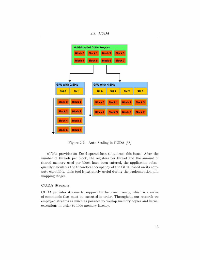
Based on the architecture of a GPU, some blocks could be scheduled dif-ferently to suit a particular hardware setting and thus improve performance.Figure 2.2 clearly indicates how blocks could be rearranged to match a dif-ferent architecture.
Automatic scalability offered by CUDA’s thread structure makes it pos-sible to divide problems into sub-problems and then solve them in parallel,regardless of the GPU specifications.
2.3.3 Kernels
Another CUDA extension to the C language is the ability to write functionscalled kernels. The main difference between CUDA kernels and C-stylefunctions is that CUDA kernels are executed in parallel on a GPU, basedon number of threads assigned to them. To avoid confusion between CUDAkernels and the mathematical kernels as used in filters (which will be dis-cussed in later chapters), throughout the rest of this work we’ll refer tomathematical kernels simply as ’kernels’ and refer to the others as ’CUDAkernels’.
Multiprocessor Warp Occupancy
Unlike CPUs, GPUs do not suffer from context-switch overhead, and workmore efficiently when they have enough threads for computation. However,there are certain trade-offs which make it difficult for programmers to har-ness the full potential of GPUs.
12
2.3. CUDA
Figure 2.2: Auto Scaling in CUDA [38]
nVidia provides an Excel spreadsheet to address this issue. After thenumber of threads per block, the registers per thread and the amount ofshared memory used per block have been entered, the application subse-quently calculates the theoretical occupancy of the GPU, based on its com-pute capability. This tool is extremely useful during the agglomeration andmapping stages.
CUDA Streams
CUDA provides streams to support further concurrency, which is a seriesof commands that must be executed in order. Throughout our research weemployed streams as much as possible to overlap memory copies and kernelexecutions in order to hide memory latency.
13

2.3. CUDA
2.3.4 Memory
While working with memories in CUDA, programmers must be aware of cer-tain considerations to assure optimal performance. Next we briefly discussthe most important and frequently encountered aspects of CUDA programs.
Bank Conflict
Shared memory is located on the same chip as multiprocessors and, as a re-sult, they have very high speed and low latency. To achieve a high bandwidthshared memory is divided into modules called banks. Since different bankscan be accessed in parallel the bandwidth increases significantly. However,it is essential that the access pattern follows the guidelines. For example,simultaneous access of the same bank by different threads may result to anissue called Bank Conflict, and should be avoided to increase throughput.
Register Spilling
There are limited number of registers available on each SM, and these reg-isters are shared among thread blocks assigned to each particular SM. Ifthe number of registers used in a CUDA kernel code exceed the availableregisters, the compiler is forced to use that thread’s local memory (whichis located in global memory; recall that it has much higher latency). Asa result, performance drops significantly. Hence, it is very important tomake sure the number of registers used are as low as possible to avoid anyperformance degradation.
Memory Coalescent
To maximize global memory throughput it’s essential to consider the accesspattern as well as the size and alignment, based on the compute capabil-ity. One important technique we used throughout our research to achievememory coalescence is padding of 2-D arrays. That is, we allocated extramemory for each row to ensure memory coalescence.
Page-Locked Host Memory
Using page-locked memory offers a few advantages such as creating higherbandwidth. Moreover, as far as GPUs are concerned, page-locked memorymakes it possible to concurrently copy data between the host and the devicememory. However, page-locked memory is a limited resource and allocatingan excessive amount would reduce the performance of the whole system.
14

2.3. CUDA
To summarize, there are numerous tradeoffs that must be consideredwhile designing algorithms or coding for GPU architectures. In the nexttwo chapters we’ll present two case studies that that indicates our approachto these limitations in industrial applications.
15

Chapter 3
Case Study: Microscopesand Micro-Pathology
Microscopes are used in many medical fields, though their limited field ofview is a major restriction for diagnosis. Currently in the field of pathology,a specimen is received and prepared onto a physical glass slide. A patholo-gist examines the slide under the microscope and makes the diagnosis basedon what is observed, and he writes a report which is sent to the physician.Unfortunately there is no easy way of capturing an image of what the pathol-ogist has observed with the microscope and associate his observations witha diagnosis. The solution currently available is to use Whole Slide Scanner(WSS) [29] which stores the image on a server for presentation or educationalpurposes. WSS is a fully automatic process; it uses a robotic microscope tocapture a large area of a slide, field by field, and then stitches the individualfields together into a single image. However, whole-slide imaging has twomajor drawbacks: First, due to the high price of this equipment, there arefew scanning centres available, most with long waiting lists (up to a week).Second, the file size of each whole-slide image is very large (at least 4GBper image), which makes sharing or archiving these images difficult.
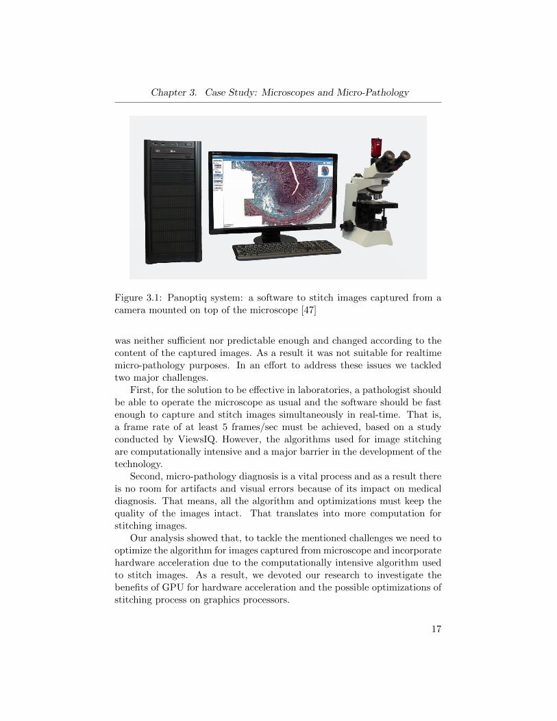
To overcome the aforementioned problems, ViewsIQ, a Vancouver-basedcompany specialized in digital medical imaging, introduced a new approachto the problem. By mounting a camera on top of a microscope and stitchingtogether the captured images (Figure 3.1), pathologists can use their existingmicroscopes in the lab to digitize their slides. As a pathologist observes aregion of interest, the system automatically captures images and stitch themtogether, forming a broad field of view for diagnosis. The system providesa real-time feedback to the pathologist while allowing more efficient useof computer storage space by capturing only the regions of interest. Thisapproach makes the analysis less time consuming and more efficient. It alsomakes referrals and second opinions on diagnosis a matter of minutes ratherthan weeks.
ViewsIQ’s initial prototype of the product (Panoptiq [48]) was able tocapture and stitch images to form a mosaic image. However the performance
16
Chapter 3. Case Study: Microscopes and Micro-Pathology
Figure 3.1: Panoptiq system: a software to stitch images captured from acamera mounted on top of the microscope [47]
was neither sufficient nor predictable enough and changed according to thecontent of the captured images. As a result it was not suitable for realtimemicro-pathology purposes. In an effort to address these issues we tackledtwo major challenges.
First, for the solution to be effective in laboratories, a pathologist shouldbe able to operate the microscope as usual and the software should be fastenough to capture and stitch images simultaneously in real-time. That is,a frame rate of at least 5 frames/sec must be achieved, based on a studyconducted by ViewsIQ. However, the algorithms used for image stitchingare computationally intensive and a major barrier in the development of thetechnology.
Second, micro-pathology diagnosis is a vital process and as a result thereis no room for artifacts and visual errors because of its impact on medicaldiagnosis. That means, all the algorithm and optimizations must keep thequality of the images intact. That translates into more computation forstitching images.
Our analysis showed that, to tackle the mentioned challenges we need tooptimize the algorithm for images captured from microscope and incorporatehardware acceleration due to the computationally intensive algorithm usedto stitch images. As a result, we devoted our research to investigate thebenefits of GPU for hardware acceleration and the possible optimizations ofstitching process on graphics processors.
17

3.1. Background Information
For the rest of this chapter we’ll introduce background and technical in-formation regarding micro-pathology and image stitching. Then we presentour analysis of the project and its components. Afterward, we describeour design and implementation of the GPU components. And finally ourevaluation of our project.
3.1 Background Information
There are a few established commercial and non-commercial products [14][15] [43] in the market to help a pathologist digitize slides, yet they sufferfrom major issues, such as large image size (capturing unnecessary partsof a slide) and slow performance. If ViewsIQ’s solution addressed thesechallenges, then Panoptiq would have an excellent standing in terms of itsusability, its hardware costs and the learning-time required to operate versusthe existing solutions. In this section we’ll provide background on availableimage stitching solutions and provide a brief technical discussion about theirbuilding blocks.
3.1.1 Image Stitching Software
There are various image stitching software available in the market. However,they are not suitable for the micro-pathology field.
On one hand, the existing software solutions are too generic for a field asspecific as micro-pathology. For example, because a microscope stage movesonly in two dimensions, and a number of these imaging products are opti-mized for use in three dimensions, the software wastes a considerable numberof unnecessary computations stitching together images in three dimensions.Moreover, some solutions demand the examining pathologist’s constant in-teraction while scanning the slides. Ideally the pathologist should not haveto deal with multiple systems.
On the other hand, alternative hardware solutions, such as whole slidescanners (WSS) [19] [27] [46] [41] [36], require significant technical knowledgeto operate, and have mechanical parts that breakdown from time to time.Unlike WSS, Panoptiq does not require significant technical backgroundor extra mechanical parts. It also helps a pathologist capture only thearea of interest and avoids unnecessary efforts to scan and store images ofunnecessary regions. WSS machines, with their complex hardware, may costup to thousands of dollars. Panoptiq, however, being a software solution,only requires off-the-shelf components, making it far cheaper.
18

3.1. Background Information
3.1.2 Image Stitching Process
There are various image stitching algorithms available and mostly theysearch any overlapping sections of the different images. Image-matching canbe classified into two groups, namely area-based and feature-based[7]. Areabased image-matching methods use intensity patterns in images. However,in feature-based methods an image is represented using feature-descriptorsinstead. Features can be key-points, edges, lines or corners. Feature-basedapproaches are immune to large amounts of ‘noise’ (unwanted, useless data)and are computationally less complex [44] which make a feature-based ap-proach suitable for this project.
In our project image-stitching consists of three major steps (Figure 3.2).First, Panoptiq detects and extracts features of the captured images througha camera mounted on top of the microscope. It then matches these featureswith other already-detected features found within the surrounding images inorder to find any overlapping parts. Finally Panoptiq calculates the displace-ment of these image fragments and forms an encompassing mosaic image.
Figure 3.2: Panoptiq’s image stitching data flow diagram
Feature Descriptor
A ’feature-detection’ algorithm, such as SIFT [10] or SURF [1], analyzes theimages received from the camera, and detects any interesting points calledfeatures by detecting any high-contrast regions such as an edge or a corner.
Next the program uses various feature-extraction methods to convert the
19

3.2. Analysis
image fragments into structures called feature descriptors, which are moresuitable for feature comparison.
This structure may represent several properties such as size, direction,coordination, etc. However, the most important one for our project is a 64or 128-dimensional vector representing the contents of the feature.
Feature Matching
To find and match similar features in the image, the software uses a Eu-clidean distance (Equation 3.1) to measure the feature-descriptor vectorsin order to calculate the level of similarity. That is, the more similar thefeatures are, the smaller the Euclidean distance between them. This processcan be computationally intensive since in micro-pathology each image mayhave around 500 features on average. That means, if there are already tenimages in the system, to find the best match, 2.5 million Euclidian distancesshould be calculated.
d(~x, ~y) =
√√√√ n∑i=1
(xi − yi)2 (3.1)
3.2 Analysis
We gained more insight into the computational and memory complexityin early stages through benchmarking and back-of-the-envelope calculation.The results helped locate the bottlenecks and analyze them for paralleliza-tion and implementation on GPU.
Our first step was to benchmark the prototype program to find the timespent on each component. Our benchmarking results showed that FeatureMatching was the costliest component in the whole stitching process (seeFigure 3.3). This indicates that we must analyze the feature-matching stepfor further parallelization possibilities.
After researching various feature matching algorithms, we decided touse exhaustive search algorithm for its accuracy, simplicity, predictable pat-terns of memory-access, and relatively easy parallelization. Having all ofthese characteristics made exhaustive search a good candidate for GPU im-plementation.
Based on a sample set of slides received from Vancouver General Hos-pital’s pathology lab, we estimated that one thousand distinct features aredetectable within any image captured from the microscope. Additionally,
20

3.2. Analysis
37.97%
31.65%
30.38%
Feature Matching
Feature Detection & Extraction
Miscellaneous
Figure 3.3: Time spend on each component for image stitching
before implementation, we completed a further computational and memoryanalysis in order to estimate the scale of the problem.
3.2.1 Computation Analysis
We benchmarked the time required to complete the image-stitching on Panop-tiq’s prototype code developed for CPU. This benchmark includes featuredetection and extraction (Figure 3.3), which takes about 50ms for every onethousand features. Based on ViewsIQ’s study the stitching process mustachieve a minimum time of five images per second or 200ms for each newimage captured. Since 50ms is spent on feature detection & extraction, thatleaves 150ms to calculate matches for maximum of six images, or 25ms foreach image.
The reason behind six images is that, the relative location of a newly-captured image is estimated by comparing its features with the ones fromunderlying images already in the system. And if the area is already coveredby other images, it is possible that the newly-captured image overlaps withsix other images as shown in Figure 3.4. All the while it’s important that theimage processing does not fall behind. It is our task to ensure the computersystem does not slow down in processing the six images in order to estimatea location.
There are two reasons we compare a captured image with six neighbour-ing images. First, a comparison of several surrounding images reduces theerror that often appears while detecting features (Figure 3.4). That is, com-paring the current image with only the last captured image increases theerror.
21

3.2. Analysis
Figure 3.4: Six neighbouring images are compared while stitching a newimage to reduce the error.
Second, one of the features Panoptiq offers is the ability to replace theareas with sharper focus automatically, called focus-replacement. This fea-ture enables a pathologist to adjust the microscope’s focus and go over thestitched images to improve the final image quality.
3.2.2 Memory Analysis
Since, we are using discrete graphics cards3 for this thesis, it is very im-portant to estimate the amount of data communication between CPU andGPU to avoid memory bottlenecks.
In our algorithm each feature descriptor vector is comprised of 128 or 64integer numbers. Each image may have around 1,000 feature and for com-parison we must transfer the vectors of at least two images to the GPU forcalculation. So the following calculation represents an approximate amountof data passed to GPU to find the best matches.
1, 000features × 2images × 128× 4B = 1MB
Furthermore, the results are stored in a 2D-array representing the in-dices of the first and the second-best match.
1, 000features × 2indices × 4B ' 8KB
3Discrete graphics cards unlike onboard graphics cards have separate memory and datashould be copied for processing.
22

3.3. Design and Implementation
With a global memory bandwidth 327.7 GB per sec, the GTX590 graphiccard could very easily handle 1MB and 8KB of data and this wouldn’t con-stitute a challenge or become a memory bottleneck. Moreover the abovevalue does not take into account the streaming optimization we have imple-mented (discussed in the next section) which hides virtually any memorylatency.
After analyzing the amount of memory transferred, it’s time to considerthe algorithms memory access pattern. Unlike the KD-Tree or similar al-gorithms, exhaustive search benefits from a very uniform and predictableaccess pattern to memory. This is very important since GPUs’ performanceare very sensitive to the access pattern and it helps us benefit from theavailable cache and reduce memory latency.
The computation and memory analysis of our matching algorithm in-dicated that it is feasible to meet the requirements as long as we manageto match a pair of feature descriptors under 25ms. The next section de-scribes how we go about design and implementation to meet this criticalrequirement.
3.3 Design and Implementation
Before implementation, it is imperative to have a clear understanding of theproject’s requirements. This was especially important for GPU-programmingsince they have Non-uniform Memory Access (NUMA) and require complexexecution models, so any minor change in requirements would hold signif-icant implications during implementation. In GPU programs, data parti-tioning is closely intertwined with the execution model. That is, any changein data partitioning or change in execution would affect the design and im-plementation of the other.
To avoid later changes, we spent a significant amount of time to clarifyingand reducing every requirement of the project. For example, instead ofvariable length descriptors on runtime, which is the approach taken in CPU-prototypes, we proposed limited fixed-length descriptors defined at compiletime.
Our research indicated that descriptors larger than 64-elements didn’timprove the quality at all on the available samples (i.e., slides received fromVancouver General Hospital). However, for future expansion of the project,we added the capability for 128-elements descriptors through a simple macrovalue change. This approach reduced the development time, it also improvedthe performance through eliminating extra computation.
23

3.3. Design and Implementation
The rest of this section consist of: memory allocation for feature descrip-tors, execution model to find the best match, and the testing strategy.
3.3.1 Data Partitioning and Memory Management
To design our algorithm we followed the parallel algorithm design explainedin literature review chapter step by step (partitioning, communication, ag-glomeration and mapping). In this section we’ll explain how we stored fea-ture descriptors in memory and how we optimized the memory access usingtexture, shared and global memory.
Feature matching requires a number of processes in order to calculatethe Euclidian distance among descriptors (Equation 3.1). Although, this isa good level for partitioning, with each two vectors assigned to one process,we found that the Euclidian distance calculation could be divided into evensmaller tasks responsible for calculating the square-difference. Figure 3.5shows the parallel design process we used.
Figure 3.5: Four steps of parallel algorithm design
24

3.3. Design and Implementation
Feature Descriptors
The feature-matching algorithm compares two sets of feature descriptorsand finds the best matches with the smallest Euclidean distance. Basedon a convention used in OpenCV4, one set of feature descriptor is calledthe ‘source’ and the other ‘destination’. Source features are compared todestination features, and the corresponding best features in destination (i.e.,least Euclidian distance) would be the indices of the returned array.
In our design every source and destination feature descriptor is pairedand corresponding values for each element of vector is assigned to a process.Based on our requirement, we have 128 processes as explained before. Tocalculate the total reduction each process requires to communicate withother processes in the pair. We have agglomerated each pair and mappedinto a GPU’s streaming processor to reduce the amount of communicationbetween each streaming multi-processor(SM).
Texture Memory
Throughout this process, the distance-values of these two sets do not change.This made it possible for us to off-load the descriptors into Texture memory.We found there were benefits to hardware optimizations, due to faster ran-dom memory access and benefits to the texture-caching mechanism. Ourinitial benchmarks shown in Figure 3.6, indicated that about 6% perfor-mance increase is achieved by offloading the descriptors to texture memoryinstead of global memory.
4OpenCV is a set of libraries, originally developed by Intel, for computer vision appli-cations
25

3.3. Design and Implementation
Figure 3.6: 6% performance improvement using texture memory
Shared Memory
As mentioned before, to reduce the amount of communication (i.e., datatransferred) we agglomerated processes into 128-element batches and as-signed them to one SM. As a result we can store the values into sharedmemory and calculate the Euclidian distance on a single multiprocessor.To employ the shared memory, one obvious way to load one vector fromeach set and perform the calculation and reduction then return the results(Figure 3.7).
26

3.3. Design and Implementation
Figure 3.7: Unoptimized memory access
However, instead we chose to optimize the code even further. We as-signed one vector to a multiprocessor’s shared memory and retained it thereuntil the remaining vectors from the other set were exhausted (Figure 3.8).
Figure 3.8: Optimized memory access
We discovered that this method reduces data transfer from global mem-ory to shared memory, and improves performance by avoiding interthread-contention the software encountered when storing the indices of the bestmatches back into global memory. That is, every multiprocessor must find aparticular destination for each descriptor’s best matches (maximum of twobest matches) within the source set and, when the matches are found, the
27

3.3. Design and Implementation
corresponding index would only be accessed by the same multiprocessor,avoiding contention as a result.
Global Memory Access Pattern
The result of comparison is a 2D-array that resides in global memory, whichholds the first and second-best matches for every vector within the sourceset. To ensure minimal performance degradation (such as false sharing) weused the cudaMallocPitch() function to pre-allocate global memory whichensures that memory is aligned and coalesced, and cudaMallocHost() topre-allocate pinned memory, padded according to cache size for better per-formance. To make sure memory access is coalesced, we have provided a setof APIs (Program 3.1) to enforce proper memory access on the host as well.
Program 3.1 API to ensure access to memory is aligned and coalescedtemplate <class T>
voidSetElement(cudaPitchedPtr matrix,intx,
inty,T value);
template <class T>
T*GetElementPtr(cudaPitchedPtr matrix,intx,
inty);
template <class T>
T GetElementValue(cudaPitchedPtr matrix,intx,
inty);
To improve the memory efficiency, we preallocated memory in both theCPU and the GPU and reused the memory contents frequently. The max-imum amount of preallocated memory is set before run-time and definedby a macro. This is possible since our research shows that number of fea-tures detected in a typical image captured from pathology slides does notexceed 1,000. This value is usually much less, because Panoptiq has filtersin the stitching pipeline that eliminates certain features based on their di-rection, size, etc. However, in order to accommodate the worst case scenarioa maximum of one thousand features is usually set.
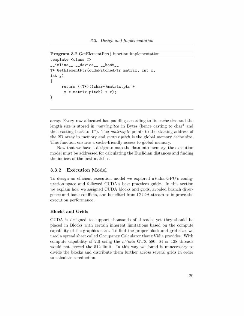
To better understand the calculation involved behind memory access seethe implementation of GetElementPtr() (Program 3.2):
The above code returns the pointer to a value stored in a padded 2D-
28
3.3. Design and Implementation
Program 3.2 GetElementPtr() function implementation
template <class T>
__inline__ __device__ __host__
T* GetElementPtr(cudaPitchedPtr matrix, int x,
int y)
{
return ((T*)((char*)matrix.ptr +
y * matrix.pitch) + x);
}
array. Every row allocated has padding according to its cache size and thelength size is stored in matrix.pitch in Bytes (hence casting to char* andthen casting back to T*). The matrix.ptr points to the starting address ofthe 2D array in memory and matrix.pitch is the global memory cache size.This function ensures a cache-friendly access to global memory.
Now that we have a design to map the data into memory, the executionmodel must be addressed for calculating the Euclidian distances and findingthe indices of the best matches.
3.3.2 Execution Model
To design an efficient execution model we explored nVidia GPU’s config-uration space and followed CUDA’s best practices guide. In this sectionwe explain how we assigned CUDA blocks and grids, avoided branch diver-gence and bank conflicts, and benefited from CUDA stream to improve theexecution performance.
Blocks and Grids
CUDA is designed to support thousands of threads, yet they should beplaced in Blocks with certain inherent limitations based on the computecapability of the graphics card. To find the proper block and grid size, weused a spread sheet called Occupancy Calculator that nVidia provides. Withcompute capability of 2.0 using the nVidia GTX 580, 64 or 128 threadswould not exceed the 512 limit. In this way we found it unnecessary todivide the blocks and distribute them further across several grids in orderto calculate a reduction.
29

3.3. Design and Implementation
According to our data-partitioning algorithm, we assigned each desti-nation feature-set to one block (i.e., grid dimension equals the number offeatures in that descriptor-vector for the destination image). Finally we cal-culate the distances compared to the source features and write back the bestmatches into global memory.
Now, to find the best matches every two feature descriptor vectors shouldbe compared based on their Euclidian distance. That implies that a reduc-tion of 64 or 128 numbers becomes a major part of the computations butthese could be executed in parallel.
Branch Divergence and Bank Conflicts
The Euclidean-distance calculation between two source and two destination-vectors consists of three major steps:
First we must calculate the square-difference element for two vectors.Second we must reduce [26] (that is, add) the results of the previous step.Third, we calculate the square-root of the reduced value. Since we are usingthe Euclidean-distance only for comparison, we could avoid the third stepentirely.
One way to perform reduction on the GPU is to arrange that currently-running threads sum the values of previously active threads, calculated bysquared-differences. In each step the number of the active threads is reducedby half, as shown in the Figure 3.9.
For example, if thread 0 is responsible for adding values in addresses 0and 1 then thread 2 is responsible for values in addresses 2 and 3. Thisapproach seems to be very simple and intuitive when writing the code sinceevery thread determines its value by reading its own ID.
30

3.3. Design and Implementation
Figure 3.9: Reduction algorithm suffering from branch divergence. [26]
However, because branch divergence reduces the performance, this methodof reduction does not conform with CUDA’s best practices. For example seethreads 1, 3, 5, and 7. These would not be reduced in the first step and theproblem is exacerbated in subsequent steps. One way to solve this issue isto arrange interleaved addressing.
Another approach is to group the threads to reduce divergence. As weshow in Figure 3.10, thread 0 would be responsible for values in 0 and 1,and thread 1 would be responsible for 2 and 3. In this way, in each warpwe are more likely to have all threads doing nothing or all are following thesame instruction.
31

3.3. Design and Implementation
Figure 3.10: Reduction algorithm suffering from bank conflicts. [26]
Although in the previous method we avoided branch divergence to somedegree, bank conflicts still existed.
For example in threads 0, 8, 16: these would have shared a memorybank during reduction. Since addition is commutable (i.e., order does notmatter) then reorganizing the access pattern would avoid any bank conflicts.We assigned each thread to access the element corresponding to its ID, andthe second element is determined simply by retrieving the next elementaccording to the number of active elements. Figure 3.11 illustrates thispattern. We can speed the process even more. Unrolling the loop responsiblefor iterating each step further reduces the computation and the number ofregisters used.
32

3.3. Design and Implementation
Figure 3.11: Reduction algorithm avoiding branch divergence and bank con-flicts. [26]
CUDA Streams
Furthermore, to achieve even higher performance and minimize latency, wedesigned a pipeline so that while the GPU calculates the matches, the CPUsimultaneously captures images and extract features. The extracted descrip-tors are then passed to the GPU and these calculated results are then copiedback to the host through CUDA streams. These operations are done entirelysimultaneously as matches are found in the GPU.
The final step is to test the component before and after integration withPanoptiq software.
3.3.3 Testing
Due to the intricacies of GPU programming we considered unit, module,integration and system level testing throughout development. We mainlyfocused on dynamic analysis to perform testing, by relying on testing ourcode through execution rather than statically analyzing it.
Unit and Module Testing
We tested nearly every unit (such as copying memory, loading data to sharedmemory, binding memory to texture or kernel-CUDA execution) and made
33

3.4. Evaluation
sure the results of the operations are as expected. To facilitate the task, weused Matlab to generate sample input and output values for our test cases.
To further test the feature matching module, we used the CPU version ofthe code which was already available and tested. We ran feature matchingcodes on both the CPU and the GPU simultaneously while, at the sametime operating the microscope and scanning the real slides. We comparedthese results on the fly to detect any inconsistencies.
Integration Testing
To test the final product we tried to simulate lab environment and used theslides received from pathology centres. However, to simulate the everydaylab environment and human interaction we performed test cases to inves-tigate the system’s behaviour in unusual scenarios such as turning off themicroscope light source or camera, obstructing the slide or manipulating thefocus.
3.4 Evaluation
We evaluated this work on high-end off-the-shelf components available atthe time. For CPU we used Intel Core-i7 2600K Quad Core 3.4GHZ SandyBridge and for GPU we obtained nVidia GTX 580 graphics card to evaluatethe performance of our CPU vs. GPU implementations. We were alsointerested in testing the scalability of our GPU code and for that we usedtwo nVidia GTX 460.
We have simulated the unrealistic extreme lab environment and gener-ated test cases that contain up to 4,000 features per slide to gain a betterunderstanding of our system, although the requirement is a maximum of1,000 features per slide. in the following sections we present the CPU vs.GPU evaluation, the scalability of our work, and how our GPU componenttransformed the bottlenecks of image stitching process.
3.4.1 CPU vs. GPU
As mentioned before, a study by ViewsIQ, indicated that 5Hz is the usability-threshold and any number above that would allow a pathologist to scan aslide faster than what they usually do. We measured the image process-ing speed in Hertz (Hz) where 1 Hz implies 1 image captured, stitched anddisplayed per second. Our GPU-coding benchmarks indicated a significantspeed increase while maintaining stability over the CPU-alone counterpart.
34
3.4. Evaluation
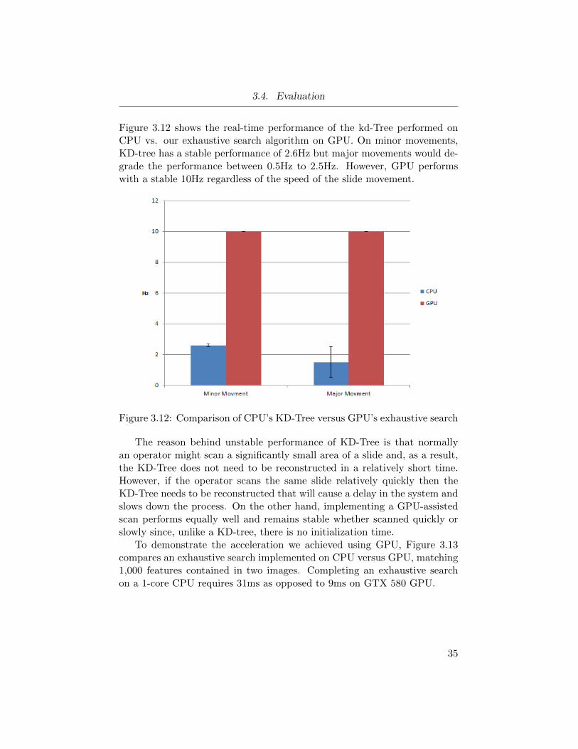
Figure 3.12 shows the real-time performance of the kd-Tree performed onCPU vs. our exhaustive search algorithm on GPU. On minor movements,KD-tree has a stable performance of 2.6Hz but major movements would de-grade the performance between 0.5Hz to 2.5Hz. However, GPU performswith a stable 10Hz regardless of the speed of the slide movement.
Figure 3.12: Comparison of CPU’s KD-Tree versus GPU’s exhaustive search
The reason behind unstable performance of KD-Tree is that normallyan operator might scan a significantly small area of a slide and, as a result,the KD-Tree does not need to be reconstructed in a relatively short time.However, if the operator scans the same slide relatively quickly then theKD-Tree needs to be reconstructed that will cause a delay in the system andslows down the process. On the other hand, implementing a GPU-assistedscan performs equally well and remains stable whether scanned quickly orslowly since, unlike a KD-tree, there is no initialization time.
To demonstrate the acceleration we achieved using GPU, Figure 3.13compares an exhaustive search implemented on CPU versus GPU, matching1,000 features contained in two images. Completing an exhaustive searchon a 1-core CPU requires 31ms as opposed to 9ms on GTX 580 GPU.
35

3.4. Evaluation
Figure 3.13: Exhaustive search comparison on CPU vs. GPU
3.4.2 Scalability
Furthermore, as shown in Figure 3.14, using two nVidia GTX 460 graphicscards we achieved near 2X (1.990%) speedup performing feature matchingon 1,000 features in two images.
13961 GPU
7782 GPUs
0 500 1000 1500 2000Time (ms)
Figure 3.14: Performance Comparison (multi GPUs)
Due to the high degree of data-parallelism in the exhaustive search algo-rithm, we developed an algorithm that allows us to use more than one GPUfor calculations. In order to employ multiple-GPUs using CUDA 3.2—thelatest CUDA version at the time of this project—we had to create a threadfor each GPU that would allocate and access device memory. This is a re-striction that is resolved in subsequent versions of CUDA. We avoid the costof ‘thread-creation’ by first creating multiple threads while initializing the
36

3.4. Evaluation
program and second, handling kernel calls through thread synchronization,which resulted in near 2X (1.990%) speedup with minor overhead.
3.4.3 Bottlenecks
As indicated earlier in this chapter, feature-matching was responsible for37.97% of the computational workload required to stitch a new image (Fig-ure 3.15). However the added computational power of a GPU reduced thatnumber to 5.77%, as shown in the Figure 3.16, leaving feature-detection andextraction as the next computationally expensive components.
37.97%
31.65%
30.38%
Feature Matching
Feature Detection & Extraction
Miscellaneous
Figure 3.15: Before introducing GPU component.
48.08%
5.77%
46.15%
Feature Detection & ExtractionFeature Matching
Miscellaneous
Figure 3.16: After introducing GPU component.
37

3.5. Conclusion
3.5 Conclusion
We discovered that a GPU search implementation not only performed betterthan a KD-Tree—one of the fastest algorithms used for feature-matching ona CPU—but a GPU-assisted search also proved to be scalable.
The value of this work is the change it brings to micro-pathology fieldand perhaps to similar disciplines. It makes it possible to easily digitizeand store images, and to create a new platform for the relatively new fieldof Telepathology that directly assists the collaboration between specialists,regardless of their geographic location. We also noticed that pathologistsusing the system usually preferred to observe the monitor directly, insteadof microscope’s eyepieces, since it was easier on the eyes and less tiring.
To conclude, using the latest GPU’s computational power has made itpossible to quickly digitize slides—the original purpose of our project— andprovided a new level of convenience and efficiency to the field of pathology.
3.6 Related Work
Concurrent with our project, Exhaustive Feature Matching for a GPU, an-other GPU based approach has been designed by Willowgarage[20] usingthe OpenCV library. A comparison of these two approaches is shown onFigure 3.17, where the number of features exceed 2000 and are repetitiveOpenCV uses techniques such as caching, thus making it more efficient thanPanoptiq. However, in our project the maximum number of features isapproximately one thousand, which OpenCV requires 23.5ms to match asopposed to just 8.34ms for our GPU-implementation.
38

3.6. Related Work
Figure 3.17: OpenCV vs. Panoptiq performance
39
Chapter 4
Case Study: 3D-Scanners
Depth perception has been one of the great challenges in the computervision industry. Several technologies have been developed to capture the3D world as accurately as possible, though, each technology has its owninherent limitations. Yet these technologies are extensively used in 3D-scanners to collect data from objects and from the environment in order tobuild virtual models. There are many applications for 3D-virtual modelsin industry; navigation, gaming and mining are a few examples. In thegaming industry Kinect has become a leading 3D-scanning device. However,the many errors Kinect generates due to its low image-depth resolution(640x480) have limited its usage by developers.
To compensate for these hardware limitations and inaccuracies, differentmethods such as the fusion of multiple sensors have been investigated [42].ApexVision, a company in Vancouver, introduced a new algorithm calledSuper-Resolution on Depth Probability (SDP) [33]. SDP makes it possibleto reduce the effects of hardware limitations and inaccuracies by up-samplingsmall 3D-scanned images using the help of larger intensity camera images.However, SDP suffers from considerable amount of computation required toimprove the digital resolution. This, of course, slows the entire process andlimits the applications.
In this work we harness GPU’s computational power and investigatepossible optimizations to make the algorithm fast enough for applicationsthat are time sensitive. ApexVision’s prototype implementation took about30sec on CPU5 to up-sample 640x480 depth image to 1280x960 using depthand colour images captured with Microsoft Kinect device. Although SDPalgorithm can be used in many fields, however, we focus on mining indus-try’s autonomous excavation[49][18] and collision detection systems[28], dueto ApexVision’s extensive research in that field. Our goal is to make it pos-sible to up-sample an image using SDP under a second and assess the GPUhardware acceleration in such systems.
For this application we have to deal with computationally intensive al-
5Benchmarked using an Intel Core-i7 2600K Quad Core 3.4GHZ Sandy Bridge proces-sor.
40
4.1. Background Information
gorithms and make sure the components used in the system are inexpensiveand easily available, similar to the Panoptiq project from the previous chap-ter. However, this algorithm has a much larger data transfers and thatincreases the risk of our implementation to become data bound and reducethe chance to effectively benefit from GPU hardware acceleration.
We used off-the-shelf components such as Kinect[12] which are abundantand relatively cheap. The main reason for using Kinect is that it capturesboth RGB colour images (1280x960) along with depth images (640x480) 30frames per second (FPS)[37] which makes it very suitable for our develop-ment. We also used GTX 590 graphics card.
The result of this work is the ability to up-sample depth images usingcolour images, both captured from Kinect, in about 125ms. This resultmade our solution feasible to be deployed for industries such as mining orstreet level mapping (GIS).
For the rest of this chapter we’ll introduce background and technicalinformation about 3d-scanners & SDP algorithm. Then we present ouranalysis and afterward the design and implementation of this application.And finally we’ll discuss the evaluation and conclusion of our project.
4.1 Background Information
In this section we provide background knowledge about types of 3D-scannersand their particular limitations. We also explain how SDP algorithm com-bines two inputs to mitigate these limitations.
4.1.1 3D scanners
3D-scanners are devices that gather data from the environment to reproducea virtual 3D-model on a computer. Our project’s focus is on non-contact 3D-scanners which do not depend on direct physical contact with the environ-ment, as opposed to contact 3D-scanners. Although non-contact approachimproves the range of collected data, however due to physical limitationsdiscuss later in this chapter, the scanning accuracy is significantly reduced.
Non-contact optical scanners[16] are divided into Passive and Active (akastructured light) scanners[13]. Active scanners use the projection of a lightbeam, such as laser, and analyze the pattern change in the reflection in orderto estimate depth (Figure 4.1). However, passive scanners rely instead uponambient light sources. Similar to cameras used for conventional photography,from which the output is a ‘colour image’, depth sensors return what’s called
41

4.1. Background Information
a ‘depth image’. This image is usually represented as a two dimensionalarray or matrix of pixels; each pixel represents depth of a specific pixel.
Figure 4.1: 3D-scanner using triangulation [5].
In addition to their inherent inaccuracies [10] active sensor performancealso suffers from external causes in the environment such as edge reflectionor transparent objects like glasses. These sensors tend to be slow for highsample rates (i.e., millions of samples) and may require minutes—versusseconds—to process an image, which in turn may introduce distortion if theobject or the scanner is also in motion.
Resolving these limitations would significantly benefit the industries us-ing 3D scanners. For example, a lot of time and money could be saved ifcollisions between the heavy equipment used in mining could be avoidedbenefiting such sensors to warn or prevent the machine operator from doinghazardous moves.
Efforts have been made to arrive at a hybrid method[8][17][25][9][51]that fuses the different approaches of capturing the environment to over-come the aforementioned problems. However, most of these methods arecomputationally intensive which defeats the purpose of the time sensitiveapplications. As mentioned before Super-Resolution on Depth Probability(SDP) is one of such methods which up-samples depth images while tak-ing edges and other possible artifacts into consideration. This represents asignificant improvement.
42

4.1. Background Information
4.1.2 Super-Resolution on Depth Probability (SDP)
In general super-resolution algorithms use low-resolution depth image dataand enhance them to obtain higher resolution images. Considering ac-tive and passive sensors restrictions, hybrid super-resolution algorithms areemerging to overcome these limitations[50][21][34], such as edge reflection.One successful fusion of sensors algorithm is SDP[24] that benefits from bi-lateral filtering 6 on depth probabilities. This approach proved to be veryeffective in up-sampling low resolution 3D depth images which reduced anumber of the edge-artifacts using colour images captured from the samescene.
The SDP algorithm has three major steps: projection, rejection andpropagation. The projection step maps the laser measurements onto thecolour image space. Rejection, lessens the effects of invalid readings fromlaser scanner by assigning weight to each measurement, such as any mis-readings caused by occlusion.
Propagation involves iteratively applying a bilateral filter to the lasermeasurements until a certain threshold is reached. This is where we turnour attention to the filtering we used for this project. We also provide infor-mation about Convolution Matrix and Cost Volume two major componentsin our filtering algorithm.
Active-Passive filtering
In order to improve the resolution or up-sample depth images, any indeter-minate values (those between valid pixels) should be assigned meaningfulnumbers. One approach is to employ basic interpolation, however, suchmethods work well only for planar surfaces, while edges would fade away.
SDP solves this problem by addressing the issue with up-sampling a low-resolution depth image to a higher level using an additional high-resolutioncolour image of the same scene. This method assumes that where edges existit is very probable that the colour intensity changes as well. Based on thisassumption, SDP takes advantage of the colour image data collected by apassive, RGB-sensor camera, which improves the image quality of the depthsensor, hence the name Active-Passive filtering. Although, this method alsoworks well with other passive sensors such as a TOF, we restrict the focusof this work to sensors that are available on the Microsoft Kinect devices7.
6A type of smoothing filter which preserves edges and reduces noise7Kinect devices have 1280x960 RGB colour sensor and 640x480 active depth sensor
43

4.1. Background Information
Convolution Matrix
SDP uses a convolution matrix to apply its filter. In filters with a weighted-average, the kernel follows a Gaussian distribution, meaning the higher theeuclidean distance between a pixel and its centre, then the lower its weight.
But SDP takes this method one step further: the kernel is responsiblefor the colour variations as well. The SDP kernel ensures that any availablecolour data is taken into consideration to avoid unwanted artifacts such asblurred edges. We used the Formula 4.3 in SDP to construct the kernel.
fc(x) = e−|x|λc (4.1)
fs(x) = e−|x|λs (4.2)
Fi,k = fc
(1
3
∑c=RGB
|Ici − Ick|).fs(‖i− k‖) (4.3)
It is important to note that unlike most kernels in which the matrix cal-culation stays the same across the image, SDP generates a unique kernel foreach pixel in the image which makes SDP particularly difficult to implementon GPU. F in Formula 4.3 is the bilateral filter in SDP where I representsthe colour image and fc and fs are colour and spatial components respec-tively. λc and λs are constants to adjust the colour and spatial sensitivityof the filter. The variables i and k represent the coordinates of two pixelsand ‖i− k‖ is the Euclidian distance between them.
Cost Volume
Next the SDP algorithm generates a 3D matrix called ‘cost volume’. Valuesin the cost volume is assigned based on the depth of the corresponding pixelas represented in Figure 4.2. That is, pixels of the similar depth are gatheredinto one layer. Then, SDP applies the bilateral filter mentioned earlier toevery layer. By using cost volume, SDP results in sharper edge definitionsas opposed to applying a bilateral filter on a single depth image.
As pointed out, the Propagation step involves iteratively applying a bi-lateral filter to each layer of the cost volume in order to propagate thedepth pixels to fill empty pixels. This process, however, is computationallyintensive and involves large number of mathematical operations, making ita good candidate for GPU-acceleration. In the next section we demonstrate
44

4.2. Analysis
Figure 4.2: SDP’s cost volume
the computation and memory analysis of SDP algorithm and its implicationsfor GPU architecture.
4.2 Analysis
In this section we assess SDP algorithm’s potential for GPU hardware ac-celeration. We looked into computational and memory analysis of the SDPalgorithm to have a glimpse of the performance we should expect and touse the results for improving the design of the system. The rest of this sec-tion we discuss the proposed design of the SDP algorithm on nVidia’s GPUarchitecture and analyze the computation and memory access behaviour ofit.
45

4.2. Analysis
4.2.1 Proposed Design
In parallel architectures such as GPU data transfer poses a great risk ofbecoming a bottleneck if not designed correctly. To avoid this issue wepropose the following design (illustrated in Figure 4.3) which is based onGPUs’ NUMA structure and incorporates SDP’s memory usage and accesspattern.
Figure 4.3: Proposed SDP design for GPU.
One aspect of concern for a data-intensive GPU application such asthis one is the transfer of data between the graphics card memory and thehost memory. The ratio of the computation time over data transfer timebecomes a defining factor on whether the code running on a GPU is going tobe data bound or not. That is, regardless of how fast a computation can beperformed on a GPU, the time required to copy the data into the GPU andback into memory might overshadow any gain. Our investigation indicatedthat kernel and image sizes mostly govern throughput.
The kernels used in SDP may vary in size yet, based on our research inApexVision, the 3x3, 7x7 and 15x15 kernels were most accurate; we foundthat larger kernels did not result in any significant improvement in imagequality. In fact the 7x7 kernels provided the best results in our lab settings,so we based our benchmarks on this particular kernel size later on.
Since we based this project on the input requirements of Kinect devices,
46

4.2. Analysis
we enhanced the depth images from 640x480 to an up-sampled 1280x960size (i.e. colour image size).
4.2.2 Computation Analysis
As shown in Equation 4.3, SDP has spatial and colour filter components.The spatial filter is simply the Euclidian distance between the kernel’s centrepixel and the surrounding pixels. This value is passed to Equation 4.2 toadjust and lessen the influence of that pixel’s value on its neighbour relativeto the centre of the kernel. It is possible to pre-calculate the values of thisfilter and store them in memory to avoid repetitive computations, since itdoes not change as the kernel moves.
SDP also calculates the colour filter component, that is, the averagedifference between each RGB-component of the kernel’s centre pixel and itsneighbouring pixels 1
3
∑c=RGB |Ici − Ick|. Afterward, to reduce the effect of
pixels which have different colour than centre pixel the value is passed toEquation 4.1.
It is important to note that unlike the spatial filter which Euclidian dis-tance is a measure for distance, colour filter measures the variations amongcolours (the average of red, green, blue components to be precise) to main-tain edges. Unlike the spatial filter, the colour filter values change as thekernel moves, which makes these values inefficient to pre-calculate.
After calculating values for each element in a kernel matrix, we performa reduction, that is, the summation of all values. To optimize this, wenormalized the values for fs in order to avoid the need to calculate anaverage every time a kernel is computed; it is sufficient simply to sum thevalues and apply the results to the appropriate element in the Cost Volume.
Our research indicated that single-precision floating point calculationswere sufficient for our purposes and, as a result, we employed 32-bit precisionacross our implementation.
4.2.3 Memory Analysis
We should note that SDP requires four sets of data for each iteration: fs,fc, Ic, and Cost Volume matrices (Formula 4.3). Except for Cost Volumeduring one set of iterations, we observed that none of the values changed.This opened certain possibilities for the use of Constant or Texture memory.
Next we implemented and analyzed the SDP algorithm to generate andmerge the Cost Volume—this time using a CPU—and observed significantrandom patterns of memory access and also noticed numerous branch di-
47

4.2. Analysis
vergences, which made this operation unsuitable for a GPU. As a result, wedecided to leave the generation and merging of the Cost Volume to be per-formed by a CPU, but pass the calculation of Cost Volume, layer by layer,to a GPU.
In an operation called the rejection phase, SDP assigns a weight to eachdepth pixel which represents the reliability of the 3D-data captured by thesensor. In propagation phase, 3D-data weight value is used to adjust thecontribution of each pixel for each iteration. For example, a typical pixelvalue obtained from a laser scanner, would be assigned a higher weight thana value derived from a TOF, such as Kinect since it’s more accurate. As aresult, the final depth image would have better and more reliable quality.
Our research indicated that depth probability, although very critical,requires very few significant figures and so depth probability can be storedin one byte, with no significant effect on the results. Therefore, to savespace and reduce the transfer time we assigned this value, along with itsassociated RGB colour values, into a single integer and then passed it to theGPU.
Finally, to make sure the program would not be memory bound, we cal-culated the amount of time SDP required to copy-in one Cost Volume layer(including one colour image) to the GPU, and also calculated the time tocopy-out the same data.
Inbound :(1280× 960)layer × 32bitfloat + (1280× 960)images × 32bitinteger ' 9.8MB
Outbound :(1280× 960)layer × 32bitfloat ' 4.9MB
Based on Kinect’s range our research indicated that we require a maxi-mum of ten layers for cost volume. However, as we will explain in detail laterin this section, by employing layer optimization and streaming, we realizedthat we could shrink memory transfer to just two layers, regardless of thetotal number of layers.
By calculating this, (9.8MB+4.9MB)×2 ' 29.4MB, we find that about29.4MB of memory is required to be transferred for the layers to the GPU. Ifwe consider global memory bandwidth of 327.7 (GB/sec) of nVidia’s GTX590, it becomes evident that the memory transfer rate would not constitutea significant time constraint when compared to the computation rate.
48

4.3. Design and Implementation
4.3 Design and Implementation
As we have mentioned in previous chapter, it is imperative to have a clearunderstanding of the requirements before designing the GPU algorithm.As a result, we researched regarding the requirements of the project tofind ways to either reduce or adjust them for better implementation andimproved performance. The design and implementation consists of memorymanagement, execution model and optimization strategies we employed toeffectively harness GPU’s computational power for SDP algorithm.
4.3.1 Memory Management
GPUs have limited amount of memory with a complex NUMA structure,so throughout our work we handled memory allocation and use with extradiligence. We made sure the memory allocation is optimized, coalescent,and reused throughout our implementation.
Minimize Memory Usage
To minimize the memory usage and data transfer time, we decided to use32-bit single floating-point precision. Furthermore, the depth probabilityof pixels didn’t require many significant figures, and as a result we couldrepresent them in one byte. That is, we mapped a range from [0..1) to[0..256). Next, in order to transfer data to a GPU, we packed this valuealong with the RGB-components of the colour image into one integer usingbit-wise operations.
Global and Texture Memory
Beside the variables for filter adjustment such as λc and λs, SDP requiresthree sets of data for filtering:
• Colour image data
• Depth image data
• Depth probability data
We found that the structure of each colour image fits well into tex-ture memory, since these values are constant across every CUDA kernel-execution. As well we found that the access pattern is cache-friendly and,since depth-probability weights are packed and stored with its associated
49

4.3. Design and Implementation
colour image, this makes memory usage more efficient. However, since weknow the depth-image values will be converted to Cost Volume and so mustchange with each iteration, we loaded these Cost Volume matrices into globalmemory instead. Based on our design each layer of the Cost Volume is thenpartitioned and processed separately by one CUDA kernel.
Image Edges
One major challenge we faced with SDP when applying a filter is the edgesof an image. That is, when a kernel works on the edge of an image somesections of the kernel try to access memory that does not exist. We mightresolve this issue either by ignoring those pixels which place the kernel offthe image (and reduce the size of the results), or by checking the location ofthe kernel before reading the value, and inserted an artificial number suchas zero.
Based on our own requirements we must not reduce the size of the image(by ignoring pixels), so it was decided to insert artificial values for these non-existent pixels. An unwelcome outcome might have been branch-divergenceand unnecessary ‘if’ conditions, which would have been a major issue if theCUDA kernel checked for coordination every time a pixel was read.
To overcome this challenge regarding depth image, we added padding(i.e. extra memory) based on the size of kernel of each layer of the CostVolume, and then assigned each memory space with zero, so the depth valueis ignored in the calculations. We also set the depth probability to zero toavoid any influence there.
Fortunately, for the colour image, values are loaded into texture memory.In this case we simply used what is called Clamp-Texture-Address-Mode, afeature of texture memory that has found considerable use in graphics andgaming applications. By using Clamp-Texture-Address-Mode, which is afeature of texture memory, we can extend the apparent edge value of animage if the kernel attempts to access any pixels beyond the edge of theimage. As a result, we managed to maintain image resolution and still avoidany branch divergence.
We went to great lengths to make sure the memory is used efficientlyand allocated in the right location within the NUMA memory structure, tomake sure the performance wouldn’t become memory bound.
50

4.3. Design and Implementation
4.3.2 Execution Model
In this section we explain the design decisions we made to make sure GPUconfiguration space and reduction process—the most complex module inour GPU component—is setup properly according to nVidia’s GPU archi-tecture.
GPU configuration space
Our experiments on different sizes of kernel indicated that the most effectivekernel size for the SDP algorithm is between 3x3 to 15x15. The reason issimple: a kernel smaller than 3x3 is not possible and a kernel larger than15x15 loses its utility due to the Gaussian function effect.
After multiplying each kernel value by the corresponding pixel, kernelvalues must be reduced. To do so, we use an algorithm similar to that usedin the ViewsIQ project. However, we faced one restriction of that algo-rithm: due to a branching issue it works best on 2n number of elements. Toovercome this limitation without resorting to branching we created kernelsthat are 2n in size. For example, in order to create a 15x15 kernel, we de-vised a 16x16 CUDA kernel. Since SDP requires the sum of its elements forreduction we initialized the extra padding elements to zero.
Reduction
Our reduction process was similar to that explained in the ViewsIQ chapter,with one difference: our reduction was done on 2-D matrix rather than 1-D.This required one change: after each row was reduced to a number, thevalues were then transferred to one row and reduced again (Figure 4.4). Byperforming these steps we avoided the problems mentioned earlier, such asbank-conflict, branch-divergence, etc.
Using an occupancy calculator (for compute capability of 2.0) we foundone hundred percent occupancy. A theoretical occupancy for a 16x16 CUDAkernel implies that there is no need to tweak our execution model in orderto get better performance. That is, there is no need to split the blocks intogrids. Thus each block calculates just one kernel.
On one hand each CUDA block, depending on the size of kernel, is either4x4, 8x8 or 16x16. On the other hand, we designed the algorithm so thateach block is responsible for just one row of data in the Cost Volume layer.In this way we ensure that each CUDA kernel must iterate on a separaterow and thus propagate the data. We assigned a row simply to be cache-coherent.
51

4.3. Design and Implementation
Figure 4.4: Moving values to one row for final reduction.
After designing the memory and model, it is time to assess the potentialsfor algorithm and code optimization.
4.3.3 Optimizations
In this section we explain the methods used for SDP algorithm’s GPU op-timizations.
SDP Algorithm Optimization
Since the Cost Volume layers are very sparse it is possible to avoid unnec-essary computations on two levels: the kernel level and the layer level.
At the kernel level, before applying the filter kernel, we examine thedepth values of this layer in parallel, and if the layers do not satisfy aminimum threshold we ignore any calculation of that iteration since therewere no valuable data to be propagated.
The objective of layer-level optimization is to take advantage of the spar-sity caused by generating Cost Volume layers.
52

4.3. Design and Implementation
We developed a module running on a CPU which analyses each layerbefore the CUDA kernel execution and partitions them, based on clusters ofsignificant depth value we found in each layer (Figure 4.5). That is, insteadof having a kernel call for each layer, we invoked one kernel call for everycluster of depth values in a layer.
Figure 4.5: Regions send to GPU for computation are indicated in boxes.
To optimize even further we used one CUDA-stream for each layer. Inthis way copying the memory contents overlaps with the computation, andwhile the previously-found sections are added to the stream for computa-tion, the partitioning code is searching for new section within the layer.The benefit is that the latency of this partitioning algorithm is significantlyreduced.
GPU Optimization
GPU registers are shared among the processors, meaning that if a variableuses four bytes of register (unlike a CPU, which only allocates four bytes)then the GPU must allocate the same amount of memory for each thread.In other words the four bytes in the GPU are multiplied by the number ofthreads. For example if a program uses ten bytes of register and a GPUkernel is processing 100 threads, then 1,000 registers are occupied. Overallthis would limit productivity enormously. If the code exceeds, for example,16KB of shared registers, then occupancy will be reduced resulting in asevere performance loss.
53
4.3. Design and Implementation
To reduce the chances of this scenario occurring and, depending on therange of the arguments passed through each CUDA kernel-execution, weused templates to avoid most runtime parameters. For example, since SDPkernel range is known (3x3, 7x7 and 15x15), we recognized that we coulduse templates to generate a function for size of each matrix. In this waythe registers were used more efficiently since the need to specify the size ofthe SDP-kernel as a function parameter was eliminated each time a differentkernel-function is executed.
As we point out in the evaluation section, mentioned optimizationshelped meet the requirements by avoiding unnecessary computations andtailoring the algorithm to GPU’s execution model. In the next chapter weexplain the testing approaches we used to make sure our implementation iscorrect.
4.3.4 Testing
Like ViewsIQ’s project we relied on dynamic analysis to test our system.The following types of tests were performed to assess the results generatedby our system accuracy and reliability.
Unit and Module Testing
To test each unit and module, we used Matlab to generate random testcases. We also generated specific test cases to verify the results of boundaryconditions.
Integration Testing
To make sure the application is working properly after we integrated allcomponents we generated test cases for boundary and irregular condition,as well as test cases for indoor and outdoor environments. Beside usingMatlab we also used values that have been captured using Kinect sensors.
Visual Testing
The last test, although not as accurate as previous two, allowed us to visu-ally inspect the images that we had up-sampled with the application. Weperformed this test by connecting a Kinect device to the application withthe help of the OpenNI library[2] and also by generating certain grid-likepatterns that that helped identify any anomalies. We looked for possible
54
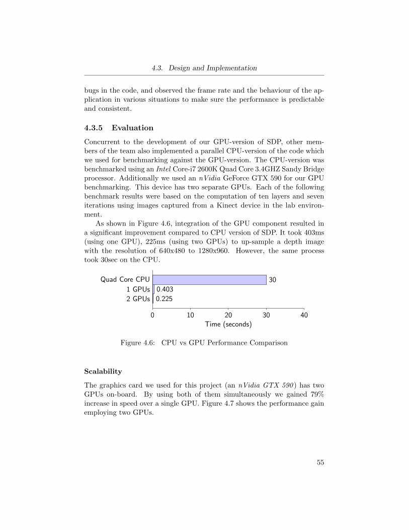
4.3. Design and Implementation
bugs in the code, and observed the frame rate and the behaviour of the ap-plication in various situations to make sure the performance is predictableand consistent.
4.3.5 Evaluation
Concurrent to the development of our GPU-version of SDP, other mem-bers of the team also implemented a parallel CPU-version of the code whichwe used for benchmarking against the GPU-version. The CPU-version wasbenchmarked using an Intel Core-i7 2600K Quad Core 3.4GHZ Sandy Bridgeprocessor. Additionally we used an nVidia GeForce GTX 590 for our GPUbenchmarking. This device has two separate GPUs. Each of the followingbenchmark results were based on the computation of ten layers and seveniterations using images captured from a Kinect device in the lab environ-ment.
As shown in Figure 4.6, integration of the GPU component resulted ina significant improvement compared to CPU version of SDP. It took 403ms(using one GPU), 225ms (using two GPUs) to up-sample a depth imagewith the resolution of 640x480 to 1280x960. However, the same processtook 30sec on the CPU.
30Quad Core CPU
0.4031 GPUs
0.2252 GPUs
0 10 20 30 40Time (seconds)
Figure 4.6: CPU vs GPU Performance Comparison
Scalability
The graphics card we used for this project (an nVidia GTX 590 ) has twoGPUs on-board. By using both of them simultaneously we gained 79%increase in speed over a single GPU. Figure 4.7 shows the performance gainemploying two GPUs.
55

4.3. Design and Implementation
4031 GPUs
2252 GPUs
0 100 200 300 400 500Time (ms)
Figure 4.7: Performance Comparison (multi GPUs)
Kernel Level Optimization
We realized benchmarking the kernel-level-optimization in isolation (notcombined with layer-level-optimization) indicated mixed performance re-sults, since it largely depended upon the environment and the shape ofthe objects being scanned. To study the behaviour, we experimented withtest case images having half of their area eligible for optimization that re-sulted in 32% performance improvement. However, if all of the area requiredcomputation then we saw that performance dropped by 26%. As a result,benchmarking kernel-level-optimizations in isolation did not suggest a defi-nite performance improvement. Also, since layer-level-optimization directlyaffects the results of kernel-level-optimization, we performed the rest of thebenchmark having both of the optimizations included and then switchedoff the kernel-level-optimization and compared the results. As shown inFigure 4.8, 15% of the performance improvement was due to the kernel-level-optimization.
15%
85%
kernel-level-optimization
layer-level-optimization
Figure 4.8: Optimization breakdown in lab environment
56

4.3. Design and Implementation
Layer Level Optimization
As suggested earlier we combined the kernel-level-optimization and the layer-level-optimization for our benchmark tests and then assessed this perfor-mance in a lab environment. The benchmarking results (Figure 4.9) showssignificant performance increase when both types of optimization were ac-tive.
13961 GPU
7782 GPUs
403(optimized) 1 GPUs
225(optimized) 2 GPUs
0 500 1000 1500Time (ms)
Figure 4.9: Performance Comparison (multi GPUs)
4.3.6 Conclusion
We have successfully implemented SDP on GPU and achieved required per-formance for the algorithm to be used in real-time applications such ascollision detection in mining industry.
4.3.7 Future Work
At the moment the load-balancing must be done statically when simultane-ously employing two or more GPUs, regardless of the size. Since we havemet the objectives laid out for our work we have not planned any futureresearch regarding the improvement of the load-balancing algorithm. Wesuggest that a possible extension to this work might be the investigation ofmethods of dynamically assigning tasks to GPUs based on the content oftheir layers.
57

Chapter 5
Conclusion
This thesis describes how graphic processor units (GPUs) can be employedto address challenges caused by the inherent limitations of two imagingdevices. Whether these shortcomings are due to optical limitations, whichnarrow a scanner’s field of view, or due to the inherent inaccuracies of active3D scanners, GPUs can play a promising role in rectifying these challengesthrough added computation. We demonstrated that a careful approach tothese challenges and following the basic software engineering methods fol-lowed by a thoughtful design that take advantage of the GPUs’ architecturehelps develop systems that address high computation needs.
With our methodology we developed GPU-code for two industry appli-cations and in the process we demonstrated that:
1. The underlying architecture of the GPU cannot be ignored in the de-velopment process. That is, we always had to consider the hardware’sstrengths and its limitations nearly for every step of the development.For example, in ViewsIQ project the ‘linear search’ was a much betterchoice than other search algorithms because its memory access pat-tern matches the GPU’s memory architecture. That also meant thatwe had to consider those algorithms that had been abandoned in thepast simply because they did not match the current CPU’s architec-ture as well as other algorithms did.
2. Although GPU-programming takes more time and effort comparedto CPU-programming, industry can accept this cost. The reason ispartially due to the current state of GPU’s exceptional computationalpower. However, when it comes to performance the industry is veryoptimistic about the increase in computation power of future GPUs.
3. GPU helped to obtain stitching capability to process images at a stablerate of 10Hz running on GPU versus an unstable rate varying between0.5 to 2.5Hz on CPU. It also made it possible to speedup SDP al-gorithm’s performance, up-sampling depth images of size 640x480 to1280x960 in 225ms as opposed to 32 seconds on CPU.
58

Chapter 5. Conclusion
Although there are many examples of successful GPU-development inacademia and industry, we want to emphasize that, in spite of its immensecomputational power, harnessing a modern GPU’s potential is a dauntingtask, and should be approached diligently.
59

Bibliography
[1] General-purpose computation on graphics hardware. http://gpgpu.
org/about. (Retrieved: October 1, 2013).
[2] Open natural interaction. http://www.openni.org. (Retrieved: july1, 2013).
[3] Open source high performance computing. http://www.open-mpi.
org/. (Retrieved: October 1, 2013).
[4] The openmp api specification for parallel programming. http://
openmp.org/wp/about-openmp/. (Retrieved: October 1, 2013).
[5] Kreon 3D. 3d laser scanner. http://www.kreon3d.com/
our-3d-scanners/3d-laser-scanner/. (Retrieved: October 1, 2013).
[6] Appentra. Parallware: Automatic parallelization of se-quential applications. http://www.appentra.com/appentra/
parallware-auto-parallelizer-source-to-source-compiler/.(Retrieved: October 1, 2013).
[7] Geetanjali Babbar, Punam Bajaj, Anu Chawla, and Monika Gogna.Comparative study of image matching algorithms. Int. J. Inform. Tech-nol. Knowl. Manage, 2(2):337–339, 2010.
[8] Haris Baltzakis, Antonis Argyros, and Panos Trahanias. Fusion of laserand visual data for robot motion planning and collision avoidance. Ma-chine Vision and Applications, 15(2):92–100, 2003.
[9] Bogumil Bartczak and Reinhard Koch. Dense depth maps from lowresolution time-of-flight depth and high resolution color views. In Ad-vances in visual computing, pages 228–239. Springer, 2009.
[10] Marco Callieri, Paolo Cignoni, Matteo Dellepiane, and RobertoScopigno. Pushing time-of-flight scanners to the limit. In VAST, pages85–92, 2009.
60

Bibliography
[11] Intel Corporation. Rapidmind. http://software.intel.com/en-us/
articles/rapidmind. (Retrieved: December 1, 2012).
[12] Microsoft Corporation. Kinect. http://www.microsoft.com/en-us/
kinectforwindows/discover/features.aspx. (Retrieved: October 1,2013).
[13] Brian Curless. From range scans to 3d models. SIGGRAPH Comput.Graph., 33(4):38–41, November 1999.
[14] Media Cybernetics. Image-pro premier software. http://www.
mediacy.com/index.aspx?page=IP_Premier. (Retrieved: August 1,2012).
[15] Media Cybernetics. Image-pro premier software. http://www.cs.
bath.ac.uk/brown/autostitch/autostitch.html. (Retrieved: Au-gust 1, 2012).
[16] Matteo Dellepiane. Grafica 3d per i beni culturali: 3dscanning. http://vcg.isti.cnr.it/~dellepiane/Corso_2012/6_
3DScanning.pdf. (Retrieved: October 1, 2013).
[17] Paulo Dias, Vıtor Sequeira, Joao GM Goncalves, and Francisco Vaz.Automatic registration of laser reflectance and colour intensity imagesfor 3d reconstruction. Robotics and Autonomous Systems, 39(3):157–168, 2002.
[18] Matthew Dunbabin and Peter Corke. Autonomous excavation using arope shovel. Journal of Field Robotics, 23(6-7):379–394, 2006.
[19] Aperio ePathology Solutions. eslide capture devices. http://www.
aperio.com/healthcare/capture. (Retrieved: August 1, 2012).
[20] Willow Garage. Opencv. http://www.willowgarage.com/pages/
software/opencv. (Retrieved: October 1, 2013).
[21] Valeria Garro, Pietro Zanuttigh, and Guido M Cortelazzo. A new superresolution technique for range data. In Proceedings of GTTI Meeting.Citeseer, 2009.
[22] Khronos Group. The openmp api specification for parallel program-ming. http://www.khronos.org/opencl/. (Retrieved: October 1,2013).
61

Bibliography
[23] Bruce M. Maggs Guy E. Blelloch. Parallel algorithms. In Algorithmsand theory of computation, 2010.
[24] Ali Haghighat-Kashani. 3D Imaging for Outdoor Workspace Monitor-ing. PhD thesis, University of British Columbia, 2011.
[25] W Hannemann, Andre Linarth, B Liu, and Gabriella Kokai. Increasingdepth lateral resolution based on sensor fusion. International Journal ofIntelligent Systems Technologies and Applications, 5(3):393–401, 2008.
[26] Mark Harris. Optimizing parallel reduction in cuda. http:
//developer.download.nvidia.com/compute/cuda/1.1-Beta/
x86_website/projects/reduction/doc/reduction.pdf. (Retrieved:August 1, 2012).
[27] GE Healthcare. Integrated digital pathology. http://www.omnyx.com/solutions/omnyx-vl4_whole-slide-scanner. (Retrieved: Septem-ber 1, 2013).
[28] NP Himmelman, JR Borthwick, AH Kashani, L Lin, A Poon, RA Hall,PD Lawrence, SE Salcudean, and WS Owen. Rope shovel collisionavoidance system. Application of Computers and Operations Researchin the Mineral Industry, 2009.
[29] Jonhan Ho, Anil V. Parwani, Drazen M. Jukic, Yukako Yagi, LeslieAnthony, and John R. Gilbertson. Use of whole slide imaging in sur-gical pathology quality assurance: design and pilot validation studies.Human Pathology, 37(3):322 – 331, 2006.
[30] Argonne National Laboratory Ian Foster. Designing parallel al-gorithms. http://www.mcs.anl.gov/~itf/dbpp/text/node14.html.(Retrieved: August 1, 2013).
[31] Intel. Automatic parallelization with intel compil-ers. http://software.intel.com/en-us/articles/
automatic-parallelization-with-intel-compilers. (Retrieved:October 1, 2013).
[32] P. Ammann J. Offutt. Introduction to software testing. CambridgeUniversity Press, January 2008.
[33] A. H. Kashani. 3d imaging for outdoor workspace monitoring. https://circle.ubc.ca/handle/2429/37670. (Retrieved: October 1, 2013).
62

Bibliography
[34] Young Min Kim and Karen Zhu. Super-resolution 3d multiview recon-struction using time-of-flight depth sensors, 2008.
[35] Jeffrey S. Vetter Kyle Spafford, Jeremy S. Meredith. Quantifyingnuma and contention effects in multi-gpu systems. Proceedings of theFourth Workshop on General Purpose Processing on Graphics Process-ing Units, 2011.
[36] MikroScan. Mikroscan d2. http://www.mikroscan.com/
whole-slide-scanners/mikroscan-d2/. (Retrieved: September1, 2013).
[37] Microsoft MSDN. Kinect for windows sensor components and specifica-tions. http://msdn.microsoft.com/en-us/library/jj131033.aspx.(Retrieved: October 1, 2013).
[38] nVidia. Cuda. http://www.nvidia.com/object/cuda_home_new.
html. (Retrieved: October 1, 2013).
[39] nVidia. Cuda c best practices guide. http://docs.nvidia.com/cuda/cuda-c-best-practices-guide/index.html. (Retrieved: August 1,2012).
[40] nVidia. Cuda c programming guide. http://docs.nvidia.com/
cuda/cuda-c-programming-guide/index.html. (Retrieved: August1, 2012).
[41] Perfekt. Digital pathology. http://www.ventana.com/product/page?view=iscan. (Retrieved: September 1, 2013).
[42] J. Davis Q. Yang, R. Yang and D. Nister. Spatial-depth super resolutionfor range images. IEEE Conference on Computer Vision and PatternRecognition, pages 1–8, 2007.
[43] Microsoft Research. Image composite editor. http://research.
microsoft.com/en-us/um/redmond/groups/ivm/ICE/. (Retrieved:August 1, 2012).
[44] Richard Szeliski. Image alignment and stitching: a tutorial. Found.Trends. Comput. Graph. Vis., 2(1):1–104, January 2006.
[45] B. B. Agarwal; M. Gupta; S. P. Tayal. Software engineering and testing.In Software Engineering and Testing, 2009.
63

Bibliography
[46] Inc. Ventana Medical Systems. iscan coreo. http://www.ventana.com/product/page?view=iscan. (Retrieved: September 1, 2013).
[47] ViewsIQ. Panoptiq. http://viewsiq.com/
digital-pathology-software-company/company-profile. (Re-trieved: August 1, 2012).
[48] ViewsIQ. Panoptiq. http://viewsiq.ca/
digital-pathology-software-products. (Retrieved: August 1,2012).
[49] Graeme Winstanley, Kane Usher, Peter Corke, Matthew Dunbabin, andJonathan Roberts. Field and service applications-dragline automation-adedade of development-shared autonomy for improving mining equip-ment productivity. Robotics & Automation Magazine, IEEE, 14(3):52–64, 2007.
[50] Qingxiong Yang, Ruigang Yang, James Davis, and David Nister.Spatial-depth super resolution for range images. In Computer Visionand Pattern Recognition, 2007. CVPR’07. IEEE Conference on, pages1–8. IEEE, 2007.
[51] Jiejie Zhu, Liang Wang, Ruigang Yang, and James Davis. Fusion oftime-of-flight depth and stereo for high accuracy depth maps. In Com-puter Vision and Pattern Recognition, 2008. CVPR 2008. IEEE Con-ference on, pages 1–8. IEEE, 2008.
64