GPS/GIS Curriculum - A Guide for Pennsylvania Agricultural … and... · 2015-07-09 · Section II...
73
GPS/GIS Curriculum A Guide for Pennsylvania Agricultural Educators 2004 Innovative Leaning Workforce Development Grant Pennsylvania Department of Education Brent M. Dahlhaus Southern Fulton High School Fulton County Area Vocational Technical School
Transcript of GPS/GIS Curriculum - A Guide for Pennsylvania Agricultural … and... · 2015-07-09 · Section II...

GPS/GIS Curriculum
A Guide for Pennsylvania
Agricultural Educators
2004 Innovative Leaning Workforce Development Grant Pennsylvania Department of Education
Brent M. Dahlhaus Southern Fulton High School
Fulton County Area Vocational Technical School

GPS Curriculum ILWD Grant
Table of Contents
Section I - Introductory GPS
Lesson One Introduction to GPS Technology Lesson Two GPS Accuracy Lesson Three Functions of a GPS Receiver – Recording Waypoints Lesson Four Functions of a GPS Receiver – Locating Waypoints Lesson Five GeoCaching Exercise
Lesson Six Differential GPS
Section II – Introductory GIS
Lesson Seven Introduction to GIS Technology Lesson Eight Exploring Geographic Careers
Lesson Nine GIS Mapping Exercise I* Lesson Ten GIS Mapping Exercise II – Latitude and Longitude**
Resource Guide
Appendix One Downloading ArcExplorer Version 9.1 Appendix Two Internet Resources
* - Requires ArcExplorer software ** - Requires ArcView and ArcVoyager software

GPS Curriculum ILWD Grant Introductory GPS Section I
Lesson One
Introduction to GPS Technology
TIME FRAME
One (1) – 41 minute instructional period
APPLICABLE EDUCATIONAL LEVEL
Introductory Agriscience Curriculum, Grade 9 (Adaptable to all Agriscience Introductory Coursework)
EDUCATIONAL OBJECTIVES
At the conclusion of this lesson, students will be able to:
1. Define the concept and science behind the development of GPS technology. 2. Identify the key components of a GPS system and define there function. 3. List the common applications of GPS technology in Agriculture.
REQUIRED MATERIALS
Instructor Lecture Points
Blackboard or Chalkboard with writing implements
Transparency #1
Overhead Projector
SESSION OUTLINE
Introductory Set Lecture Notes 1
Transparency #1 Example 1 Wrap Up Activity 1
Day Two – Introductory GPS Quiz #1

LECTURE POINTS
Introductory Set – Probing Question “Have you ever gone fishing and found that perfect spot? It was the best location,
and the fish were biting all day long. (Solicit student response) Unfortunately for you, you can’t find your way back! What could you do to mark your favorite spot? How can you find your way back each and every time you want to nab that big fish? (Solicit student response)…… The answer is GPS or a Global Positioning System.
Lecture Notes 1
What is GPS and how was it developed? Definition of GPS
GPS – GPS stands for Global Positioning System and is the science of using satellite and computer technology to determine a precise geographical location on the earth’s surface
GPS Technology Development
GPS technology was developed by the Department of Defense to be used for military applications.
Technology has spread to the private sector and is now used for commercial and recreational applications.
What are the key components of a GPS System? GPS Components
GPS satellite- Twenty four (24) satellites are in orbit roughly 11,000 miles
above the earth’s surface. - A satellite transmits a signal to earth containing the satellite
number and the time in which the satellite signal was sent. - Each satellite is equipped with an extremely precise clock that
keeps time within three nanoseconds or 0.000000003, or 3 billionths of a second.
GPS receiver- A GPS receiver receives a signal from a satellite and calculates
the receiver’s geographical location. - A GPS receiver does not “talk” to a satellite. It uses
mathematics to determine its location. - The accuracy of a GPS receiver’s measurement is directly
related to the quality of its internal clock. - (Transparency #1) The receiver calculates the difference
between the time in which the signal from the satellite was sent and the time it was received.
Time of travel = time signal received – time signal sent

- The calculated time of travel is them multiplied by the speed of light (186,000 miles per second) to mathematically determine the distance from the satellite to the receiver.
Distance to satellite = time of travel * speed of light
(Work through separate example – if necessary)
Example 1:
If it took .065 second for the signal to travel from the satellite to our receiver,
how far are we from the satellite?
Distance to satellite = time of travel * speed of light
Distance to satellite = .065 second * 186,000 miles/second
Distance to satellite = 12,090 miles
Wrap Up Activity 1
We have defined GPS and its key components, now what do you think you could use this
technology for?
Have students break up into groups of three or four students. Students have five - ten minutes to brainstorm. A presenter from each group will be asked to present their findings.
1. Challenge students to brainstorm four (4) practical applications of GPS technology. Answers can include commercial as well as recreational activities.
2. All answers must be presented with descriptive text. ie. A farmer can locate the precise location of his soil sample and return to that location year after year.
3. Have students present their brainstormed applications to the class.
EVALUATION MODEL
Beginning of Day # 2 –Introductory GPS Quiz #1
EXTENSIONS
Extensions for Lesson 1 Research1) Encourage students to research the history of the development of GPS
technology, from early military applications to modern recreational uses.

2) Have students define local points of interest in there community that they would like to locate geographically using a GPS system. Plan to locate them in future lessons.
Student Preparations for Lesson 2 Probing Question
1) We have brainstormed different uses of GPS technology. Do you think there might be different types of GPS receivers? How might they differ?
2) We have defined how a receiver can determine its distance from a satellite. How do we then determine a precise location? What else might be needed and why?
Additional Resources Websites of Interest – general GPS Information
www.trimble.com/gps/
www.garmin.com/aboutGPS/
www.magellangps.com/
Introductory GPS – Quiz #1 Name: ____________________
Multiple Choice - Place the letter of the correct answer in the space provided:
__________ 1) The speed of light is equal toa) 186,000 feet per second b) 150,000 miles per hour c) 186,000 miles per hour d) 210,000 feet per second
__________ 2) The quality or accuracy of a GPS receiver’s measurement is primarily dependent upon the?
a) location of the satellite. b) quality of the internal clock.c) time of day in which the measurement was taken. d) height of the individual taking the measurement.
Short Answer - Answer the following in complete sentences:
3) Define GPS:
4) What is the mathematical equation used to determine distance to a satellite?
5) What two pieces of information is the GPS unit receiving from a satellite?

Cal
cula
ting D
ista
nce
A r
ece
ive
r ca
lcu
late
s d
ista
nce
to
th
e S
ate
llite
ba
se
d o
n t
ime
. (
Tw
o S
tep
s)
1)
Tim
e o
f tr
ave
l =
tim
e s
ignal re
ceiv
ed –
tim
e s
ignal sent
2)
Dis
tance to s
ate
llite
= tim
e o
f tr
avel *
speed o
f lig
ht
Speed o
f Lig
ht
= 1
86,0
00 f
eet/second
(radio
waves tra
vel at a c
onsta
nt)
Tra
nspare
ncy #
1

GPS Curriculum ILWD Grant Introductory GPS Section I
Lesson Two
GPS Accuracy
TIME FRAME
Two (2) – 41 minute instructional periods
APPLICABLE EDUCATIONAL LEVEL
Introductory Agriscience Curriculum, Grade 9 (Adaptable to all Agriscience Introductory Coursework)
EDUCATIONAL OBJECTIVES
At the conclusion of this lesson, students will be able to: 1. Describe the process in which a GPS receiver determines a mathematically
correct geographical position. 2. Define selected geographical and GPS terms as they pertain to GPS data
collection.3. List major factors that can contribute to data error and miscalculations of
geographical locations.
REQUIRED MATERIALS
Introductory GPS – Quiz #1
Instructor Lecture Points 2
Blackboard or Chalkboard with writing implements
Transparency #2-4
Overhead Projector
Hand Held GPS Receiver – fully charged and initialized (refer to operators manual for initialization instructions)

SESSION OUTLINE
Introductory Set – Introductory GPS Quiz #1 Lecture Notes 2
Transparency #2
Transparency #3
Transparency #4 Terms and Definitions Wrap Up Activity 2
LECTURE POINTS
Introductory Set – Introductory GPS Quiz #1 A quiz is provided and may be used at this time. The quiz is designed to evaluate the level of knowledge acquired during the first lecture. Further review prior to or after the Quiz administration may be required.
Lecture Notes 2
How does a GPS Unit determine a precise geographical location? Geographical location – single satellite
Given the time in which it took for the satellite signal to reach the receiver, and the given value of the speed of light, one can determine their distance to the designated satellite.
(Transparency #2) The calculated distance to the single satellite fails to provide a specific geographical location. A single satellite provides only a single sphere or distance. The receiver can thus be located anywhere along that sphere (equidistant to the satellite).
Geographical location – two satellites
(Transparency #3) Two satellites fail to provide a specific geographical location as well. Two satellites provide two spheres or distances. The area in which the two spheres cross provides possible locations. This area contains a large sample of possible locations, too many to decipher a precise location.
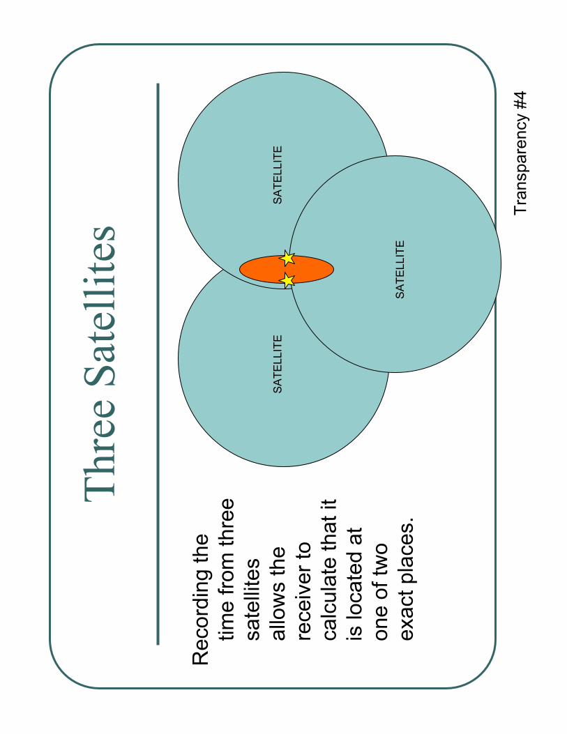
Geographical location – three satellites
(Transparency #4) Three satellites further narrow the possible geographical locations to two possible locations. The area in which the three spheres cross provides two possible locations in which one is geographically erroneous.
A GPS receiver that is properly configured will eliminate the erroneous data point based on its initial set up (second point may be at an unrealistic elevation or not close to the earth’s location).
Most GPS units can therefore determine a geographical location based on the signal of three satellites.

Is the signal of three satellites enough to make a mathematically correct determination of
your location? In order to determine a mathematically correct geographical location, GPS units
require at minimum of four satellites.
Four satellites will determine an x, y and z coordinate (latitude, longitude, and elevation).
Now that we know our location, what does this all mean? (Terms and Definitions) The geographical location generated by the GPS receiver can now be stored in the unit for further reference and use. The location after being stored is referred to as a Waypoint.
Waypoint – a location saved in the receiver’s memory which is obtained by entering data, calculating data or saving a current position.
The geographical location or waypoint can be stored in numerous formats. The format that you select will be referred to as the Coordinate System.
Coordinates – the waypoint will reflect specific geographical data. The coordinates are a unique numeric or alphanumeric description of the position.
The most frequently used coordinate systems are the Latitude/Longitude system and the UTM system.
Latitude/Longitude-o Latitude – The angular distance north or south of the equator. o Longitude – The angular distance east or west of the prime
meridian (Greenwich Meridian).
UTM – Universal Transverse Mercator metric grid system used on most large and intermediate scale land topographic charts and maps.
GPS receivers allow the operator to select the coordinate system in which they choose to work with. This may be altered during data collection. The system that the operator selects is typically dictated by the type of manipulation that the data will undergo in the end. In most cases, students are most familiar with the Latitude/Longitude system and thus this system is chosen for data collection purposes.
Not all geographical measurements are correct. What plays a role in the accuracy of our
measurements?
Accuracy of geographical positions is highly dependent on the following:

Accuracy of the receiver clock – this is the largest factor in accuracy. The more precise the clock, the more precise the location. Most recreational GPS units are accurate within 15 meters of the correct geographical location. Mapping GPS systems provides for accuracy within approximately 1.5’, while Survey GPS systems can be as accurate as ¾”. As the accuracy of the clock increases so does the cost. Survey GPS units can cost upwards of $75,000.
Weather – Inclement weather and overcast or cloudy days can alter the direction and speed of signals from satellites. The clearer the day, the easier it is to collect data with ease and accuracy.
Overhead Obstructions – Items that are located between the receiver and the satellite obscure the proper reception of the satellite signal and can result in faulty measurements. If data is to be collected in an area with overhead obstructions, specific alterations to the data must be made in order to ensure extreme accuracy. For recreational purposes this is not traditionally an issue.
Wrap Up Activity 2
We have discussed data collection and the need for an acceptable number of satellites.
Now let’s look at a GPS receiver and determine the amount of satellites available to us.
Utilize a hand held GPS receiver to demonstrate the reception of satellite signals. This portion of the activity must be done outdoors, as the receiver will not work effectively in an enclosed space. It is recommended to use a single receiver to demonstrate this information as students are not yet prepared to use the receivers on an individual basis.
Utilize the Status Screen, or screen that graphically shows the satellite locations, to demonstrate the following:
Satellite Positions
Satellite Number
Satellite Signal Strength
Note to students that on most units the screen will change to a Position Screen when an adequate number of satellites (enough to determine a location) are received. The Position
Screen will display the Coordinates for that specific geographical location
This brief demonstration will energize the students to participate in a hands on activity as demonstrated in the next Lesson.
EVALUATION MODEL
Beginning of Day # 3 –Introductory GPS Quiz #2

EXTENSIONS
Extensions for Lesson 2 1) Have students determine what section of the UTM Coordinate system they currently reside in. This information can be found through a simple internet search. Have students record this information for possible future use in later Lessons.
Teacher Preparations for Lesson 3 1) Before beginning Lesson #3, properly initialize all units and fully charge all batteries. Check operation of all units before dispersing to students.

Introductory GPS – Quiz #2 Name: ____________________
Multiple Choice - Place the letter of the correct answer in the space provided:
1) ___________ is the angular distance east or west of the prime meridian. a) Latitude b) Landmark c) Altitude d) Longitude
2) ____________ is allocation saved in a unit’s memory. a) UTMb) Routec) Waypointd) Datum
Short Answer - Answer the following in complete sentences:
3) How many satellite signals are required to determine a mathematically correct geographical location?
4) Define two practical uses of GPS technology?
5) What naturally occurring event can cause an error in GPS measurements?

On
e S
atel
lite
Record
ing the tim
e fro
m o
ne s
ate
llite
allo
ws the r
eceiv
er
to
calc
ula
te h
ow
far
aw
ay it is
fro
m the s
ate
llite
. T
hus the
receiv
er
know
s it is
locate
d s
om
ew
here
on the s
phere
.
Tra
nspare
ncy #
2
SA
TE
LL
ITE

GPS Curriculum ILWD Grant Introductory GPS Section I
Lesson Three
Functions of a GPS Receiver – Recording Waypoints
TIME FRAME
One (1) – 41 minute instructional period
APPLICABLE EDUCATIONAL LEVEL
Introductory Agriscience Curriculum, Grade 9 (Adaptable to all Agriscience Introductory Coursework)
EDUCATIONAL OBJECTIVES
At the conclusion of this lesson, students will be able to: 1. Describe the process in which a GPS receiver records waypoints. 2. Demonstrate the use of a Users Manual to manipulate the use of a GPS
receiver.3. Demonstrate how to record waypoints and alter the data that is recorded.
REQUIRED MATERIALS
Introductory GPS – Quiz #2
Instructor Notes – Hands on Activity #1
Hand Held GPS Receivers – fully charged and initialized (refer to operator’s manual for initialization instructions)
GPS Receiver Users Manual (enough for each team)
SESSION OUTLINE
Introductory Set – Introductory GPS Quiz #2 Hands on Activity #1 Wrap Up Activity #3

LECTURE POINTS
Introductory Set #1 – Introductory GPS Quiz #2 A quiz is provided and may be used at this time. The quiz is designed to evaluate the level of knowledge acquired during the second lecture. Further review prior to or after the Quiz administration may be required.
Introductory Set #2 – Review of Prior Knowledge
We ended the previous lecture with a demonstration of the ability of a GPS receiver to recognize and receive satellite signals. It may be helpful to review the function of the Status and the Position Screens.
Review:We utilize the Status Screen, or screen that graphically shows the satellite locations, to demonstrate the following:
Satellite Positions
Satellite Number
Satellite Signal Strength
Most units will change screens to a Position Screen when an adequate number of satellites (enough to determine a location) are received. The Position Screen will display the Coordinates for that specific geographical location
(A reminder: This portion of the activity must be done outdoors, as the receiver will not work effectively in an enclosed space.)
Hands on Activity #1 – Logging Waypoints (The following exercise was created to be general in nature due to the fact that not all GPS equipment utilizes the same terminology and functions. Please refer to your GPS Unit’s User Manual for detailed operational instructions.)
Purpose of Exercise: Students will be introduced to the GPS receiver and it’s operation and will work in small groups to log or record a Waypoint. Students will demonstrate their ability to record necessary data and alter such data as needed.
Advanced Preparations: Ensure that all units (receivers) are fully charged and initialized.
Prior to distributing units to students review the following expectations: a) The units are not toys. They are delicate measuring instruments. They are
not to be dropped, swung on the lanyard, or abused in any manner. b) Review your schools policy on abuse of equipment and replacement costs
incurred by the student for such abuse.

c) The curiosity of students to explore the many screens of a GPS unit can lead to management problems. When providing instruction, have all students hold units at there side (dangle freely on the lanyard) and face towards the instructor.
Activity Steps: (all instructions are generic in nature; please substitute your GPS unit’s terminology when necessary) (The word Pause is added at the end of steps that the entire group should complete prior to moving to the next step)
1. Break students into groups of two or three students. More than three students in a group tends to lead to idle hands and possible problems.
2. Provide each group with a Users Manual or supporting documentation for the operation of the GPS receiver.
3. Have students power up their units by pressing the power key. Most units will require you to press an additional key to enter the screen menus. (Pause)
4. The GPS unit, once started, should change to the position screen. Review the presence of Satellite Positions and the indication of Satellite Signal Strength. (Pause)
5. Once the receiver has computed a fixed position, the Status Screen will be replaced by the Position Screen. Depending on weather conditions, this may take seconds to minutes. (Pause)
6. Instruct students to utilize the Users Manual to identify the information provided on the Position Screen. Specific information concerning the computed position of the GPS receiver and basic navigational data is provided in this screen. Note that due to error in measurements not all students will have the exact same coordinates; however they should be relatively close. (Pause)
7. Have students move to an alternate location and note that the computed position changes. Note also that the GPS receiver is not like a compass, in that it takes time to compute its geographical location. (Pause)
8. Using the Users Manual, identify the key to mark a location. (To save time you may want to have identified this for yourself prior to the lecture). Instruct students that by depressing this key you record the geographical information into the receivers memory, thus creating a Waypoint. Select a location and mark it as a Waypoint. I would recommend choosing a recognizable feature that the students can identify. For most receivers the screen will allow you to alter the recordable data to include a message or label. Utilize your Owners Manual to manipulate this screen. (Pause)
9. Have each team show you there display prior to pressing the enter key. Once each team has logged a Waypoint, have them power down the unit and store it for future use. Specific shut down procedures are described in the Users Manual.
Wrap Up Activity 3 While students are powering down there receivers, review the following information through questioning of the teams:
What key powers up the GPS Receiver?
A recorded geographical location is referred to as a?
What key on the GPS receiver records a waypoint?

What data can we alter before storing a waypoint?
What key shuts down the GPS receiver?
EVALUATION MODEL
Beginning of Day # 4 – Observe teams power up their assigned GPS receiver. Provide corrective instruction as needed.
EXTENSIONS
Extensions for Lesson 3 1. Have students recall the local points of interest that they defined in Lesson #1
Extensions and allow them to work independently to record Waypoints for the chosen locations.
Teacher Preparations for Lesson 4 1. In Lesson #4 we will be utilizing the receiver to return to a Waypoint that was
previously recorded. Ensure that all teams have a waypoint recorded from previous instruction, and that it is properly identified with a label.
2. Review the section of the Users Manual that details the use of Navigational Screens and the recalling of a stored Waypoint. Most units have multiple Navigational Screens, so you will have to select a screen that you will utilize to return to a waypoint in the next lesson. Familiarize yourself with the use of the Navigational Screen.

Introductory GPS – Quiz #3 Name: ____________________
Multiple Choice - Place the letter of the correct answer in the space provided:
__________ 1) A theme is a combination of what two pieces of information? a) Data and Time b) Location and Data c) Time and Location d) Time and Patterns
__________ 2) Multiple themes can be combined in layers to form a? a) Quadrangleb) Picturec) Mapd) Pattern
Short Answer - Answer the following in complete sentences:
3) Define GIS:
4) What possible implications do GIS and its mapping capability have on the production of crops?
5) If we were able to compare two maps of the same area with data taken at two different decades, what might we be able to infer from the comparison?

Tw
o S
atel
lite
s
Record
ing the tim
e fro
m tw
o s
ate
llite
s a
llow
s the r
eceiv
er
to c
alc
ula
te that it is locate
d s
om
ew
here
on the c
ircle
of
inte
rsection b
etw
een the tw
o s
phere
s.
Tra
nspare
ncy #
3
SA
TE
LL
ITE
SA
TE
LL
ITE
GPS Curriculum ILWD Grant Introductory GPS Section I
Lesson Four
Functions of a GPS Receiver – Locating (Go To) Waypoints
TIME FRAME
One (1) – 41 minute instructional period
APPLICABLE EDUCATIONAL LEVEL
Introductory Agriscience Curriculum, Grade 9 (Adaptable to all Agriscience Introductory Coursework)
EDUCATIONAL OBJECTIVES
At the conclusion of this lesson, students will be able to: 1. Demonstrate the use of a Users Manual to manipulate the use of a GPS
receiver.2. Demonstrate how to locate (go to) waypoints and utilize the receiver to
return to a designated location.
REQUIRED MATERIALS
Instructor Notes – Hands on Activity #2
Hand Held GPS Receivers – fully charged and initialized (refer to operator’s manual for initialization instructions)
GPS Receiver Users Manual (enough for each team)
SESSION OUTLINE
Introductory Set – Open Questions to Teams Hands on Activity #2 Wrap Up Activity #4

LECTURE POINTS
Introductory Set – Review of Prior Knowledge
Review:While students are powering up there receivers, review the following information through questioning of the teams:
What key powers up the GPS Receiver?
A recorded geographical location is referred to as a?
What key on the GPS receiver records a waypoint?
What data can we alter before storing a waypoint?
What key shuts down the GPS receiver?
Hands on Activity #2 – Relocating Waypoints (The following exercise was created to be general in nature due to the fact that not all GPS equipment utilizes the same terminology and functions. Please refer to your GPS Unit’s User Manual for detailed operational instructions.)
Purpose of Exercise: Students will be re-introduced to the GPS receiver and its operation, and will work in small groups locate a Waypoint.
Advanced Preparations: Ensure that all units (receivers) are fully charged and initialized.
Prior to distributing units to students review the class expectations in regards to proper use of equipment.
Activity Steps: (all instructions are generic in nature; please substitute your GPS unit’s terminology when necessary) (The word Pause is added at the end of steps that the entire group should complete prior to moving to the next step)
1. Break students into groups of two or three students. More than three students in a group tends to lead to idle hands and possible problems.
2. Provide each group with a Users Manual or supporting documentation for the operation of the GPS receiver.
3. Have students power up their units by pressing the power key. Most units will require you to press an additional key to enter the screen menus. (Pause)
4. Once the unit has established its geographical location, instruct the teams to utilize the Users Manual to identify the key to relocate a Waypoint. Follow the Users Manual to recall the Waypoint that was stored in the previous lesson. Have teams start this process in a location that differs from the stored Waypoint.(Pause)
5. Once the Waypoint is recalled, utilize a Navigational Screen to return to the designated location from the previous day. Instruct teams on the use of the Navigational Screen of your choice, as most receivers offer multiple screens. (Pause)
6. Allow students to utilize the Navigational Screens to return to the designated Waypoint. Have students note the accuracy of their receiver (distance to location when receiver indicates arrival at the Waypoint). (Pause)

7. Once a team demonstrates proficiency in their ability to select and relocate a Waypoint, challenge teams to record an additional four (4) Waypoints with distinct geographical differences. Reaffirm the importance of a precise label for identification purposes.
8. Have teams trade receivers and attempt to locate another teams four (4) Waypoints as designated in Step #7. Have teams note the accuracy of their receiver as they attempt to relocate the designated Waypoints.
9. Once a team has relocated all four (4) Waypoints, have the teams power down the unit and store it for future use. Follow the specific shut down procedures are described in the Users Manual.
Wrap Up Activity 4 While students are powering down their receivers, review the following information through questioning of the teams:
What major factors affected the accuracy of your GPS receivers today?
What was the most difficult part of utilizing the Navigational Screens to relocate your Waypoints?
How could the individual who records the Waypoint make the location easier for the next team?
What are examples of how this technology could be used in a real world application?
EVALUATION MODEL
Beginning of Lesson #5 - Observe teams as they power up their assigned GPS receiver and mark a designated Waypoint. Provide corrective instruction as needed.
EXTENSIONS
Extensions for Lesson 4 1. Have students explore the alternate Navigational Screens. Utilize the Users
Manual to manipulate the alternate Navigational Screens to locate designated Waypoints.
Teacher Preparations for Lesson 5 1. In Lesson #5 we will be utilizing the receiver to relocate Waypoints. Ensure that
all teams have demonstrated the ability to record and relocate Waypoints in a proficient manner.
2. Determine the geographical location (longitude and latitude) of designated Waypoints or Caches located throughout the property. Record locations and reference points/markers for use in Lesson #5. If desired, deposit trinkets or recognizable items at each location. Utilize the Lesson #5 “GeoCaching Locations Chart” to record data for future student use.
Thre
e S
atel
lite
s
Record
ing the
tim
e fro
m thre
e
sate
llite
s
allo
ws the
receiv
er
to
calc
ula
te that it
is locate
d a
t
one o
f tw
o
exact pla
ces.
Tra
nspare
ncy #
4
SA
TE
LL
ITE
SA
TE
LL
ITE
SA
TE
LL
ITE
SA
TE
LL
ITE

GPS Curriculum ILWD Grant Introductory GPS Section I
Lesson Five
GeoCache – A GPS Treasure Hunt Activity
TIME FRAME
One (1) – 41 minute instructional period* *A second instructional period may be required depending upon location and number of Caches.
APPLICABLE EDUCATIONAL LEVEL
Introductory Agriscience Curriculum, Grade 9 (Adaptable to all Agriscience Introductory Coursework)
EDUCATIONAL OBJECTIVES
At the conclusion of this lesson, students will be able to: 1. Demonstrate the use of a Users Manual to manipulate the use of a GPS
receiver.2. Demonstrate how to locate (go to) waypoints and utilize the receiver to
return to a designated location.
REQUIRED MATERIALS
Instructor Notes – Hands on Activity #3
Designated markers and geographical locations of Caches
Hand Held GPS Receivers – fully charged and initialized (refer to operator’s manual for initialization instructions)
GPS Receiver Users Manual (enough for each team)
SESSION OUTLINE
Introductory Set – Open Questions to Teams Hands on Activity #3 Wrap Up Activity #5

LECTURE POINTS
Introductory Set – Review of Prior Knowledge
Review:While students are powering up there receivers, review the following information through questioning of the teams:
What key on the GPS receiver records a waypoint?
How does an operator alter the data of a Waypoint before storing?
What key or keys on the GPS receiver are utilized to relocate a waypoint?
What is the estimated accuracy of the GPS unit that they are operating?
Hands on Activity #3 – GeoCaching (The following exercise was created to be general in nature due to the fact that not all GPS equipment utilizes the same terminology and functions. Please refer to your GPS Unit’s User Manual for detailed operational instructions.)
Purpose of Exercise: Students will be re-introduced to the GPS receiver and the ability to enter geographical locations. Students will work in small groups locate Waypoints or Caches.
Advanced Preparations: Ensure that all units (receivers) are fully charged and initialized.
Prior to distributing units to students review the class expectations in regards to proper use of equipment.
Print out the “GeoCaching Locations Chart”, created prior to this exercise, which lists the geographical location (longitude and latitude) of designated Waypoints or Caches located throughout the property.
Activity Steps: (all instructions are generic in nature; please substitute your GPS unit’s terminology when necessary) (The word Pause is added at the end of steps that the entire group should complete prior to moving to the next step)
1. Break students into groups of two or three students. More than three students in a group tends to lead to idle hands and possible problems.
2. Provide each group with a Users Manual or supporting documentation for the operation of the GPS receiver and the GeoCaching Locations Chart created previously.
3. Have students power up their units by pressing the power key. Most units will require you to press an additional key to enter the screen menus. (Pause)
4. Once the unit has established its geographical location, instruct the teams to utilize the Users Manual to mark a Waypoint. (Pause)
5. Once the Waypoint is marked, utilize the edit features of the receiver to alter the geographical location of the Waypoint to match the locations as provided in the

GeoCaching Locations Chart. The same process used to rename a Waypoint in previous lessons can be utilized to change the longitude and latitude of a location.
6. Have all teams enter the data for location #1 as provided. Instruct students to name the Waypoints according to the chart and create a message that will describe the trinket or Cache item. Before each team saves their first Waypoint check all units to ensure that locations, data, and name are correctly changed. (Pause)
7. Once Location or GeoCache #1 is correctly entered, instruct teams to continue to enter the data as provided. (Pause)
8. Recalling the procedures used in Hands On Activity #2, instruct all groups to utilize the Go To functions of their receivers to locate the locations (GeoCahes) that they have manually entered. Be sure to designate start points for each group so that students may work independent of other groups. Instruct all groups to record the accuracy of their GPS receiver upon locating the trinket or Cache.Accuracy will be noted as the distance the receiver indicates it must still travel even when the location of the receiver is correct.
9. Encourage groups to utilize the various Navigational screens when attempting to locate the Caches. They may find one screen easier to work with than another.
10. Once a team has located all designated trinkets or Caches, have the teams turn in their GeoCaching Locations Chart and power down the unit. Follow the specific shut down procedures are described in the Users Manual.
Wrap Up Activity 5 While students are powering down their receivers, review the following information through questioning of the teams:
What major factors affected the accuracy of your GPS receivers today?
Could you have operated the receiver in any other manner that would have improved your accuracy?
Which Navigational screen did you find most helpful when attempting to locate a cache?
What are examples of how this technology could be used in a real world application?
EVALUATION MODEL
Given a period of time for evaluation, roughly 5-8 minutes per student, provide a scenario in which each individual student must operate the GPS receiver to perform a designated function. Use this evaluation method to ensure that all students have adequately participated in each activity and have gained the depth of knowledge to effectively operate a designated receiver. Customize this evaluation tool to effectively evaluate the depth of knowledge that you have individually instructed.
EXTENSIONS

Extensions for Lesson 5 1. With oversight of the instructor, research and utilize internet based GeoCaching
websites. www.geocaching.com Identify caches located in your county or region, determine the geographic information needed to locate the item, program a GPS receiver, and work with students to locate items.
2. Utilizing the internet based GeoCaching websites, establish a Geocache at your school or in an approved location within your county. Monitor the amount of visits to the Cache and provide upgrades or replacements as necessary.
Teacher Preparations for Lesson 6 1. In Lesson #6 we will be utilizing a formal instruction within the classroom
setting. Ensure the availability of required instructional materials and classroom space.
GPS Curriculum ILWD Grant Introductory GPS Section I
Lesson Six
Differential GPS
TIME FRAME
Two (2) – 41 minute instructional periods. One for lecture and one for a designated activity.
APPLICABLE EDUCATIONAL LEVEL
Introductory Agriscience Curriculum, Grade 9 (Adaptable to all Agriscience Introductory Coursework)
EDUCATIONAL OBJECTIVES
At the conclusion of this lesson, students will be able to: 1. Define Differential GPS and the mathematical process in which the error
in measurements are calculated. 2. Describe how the system improves GPS accuracy. 3. Outline the ways in which Differential GPS are implemented in
production agriculture and various field of natural resources management.
REQUIRED MATERIALS
Instructor Lecture Notes #6
Blackboard or Chalkboard with writing implements
Copies of “GPS Impact” Activity Guide.
Computers with Internet access.
SESSION OUTLINE
Introductory Set Lecture Notes #6
o Transparency #5 Day Two - Hands on Activity #4 “GPS Impact”
LECTURE POINTS
Introductory Set – Probing Questions “By now, we have all had the opportunity to use basic GPS skills in locating geographical locations. However, as most of you have seen, the accuracy of our instruments is very limited at times.
1) Do you think that the accuracy we have obtained in our previous exercises was sufficient or acceptable?
2) Can you picture possible scenarios in which our accuracy would not be acceptable? What would they be?
3) What level of accuracy do you think is required for recreational activities such as finding your favorite fishing spot? What about a scientist finding their research site? Is the same accuracy acceptable?
Lecture Notes #6
The accuracy of our GPS receivers is highly dependent on a variety of conditions. Such
conditions will impact ones ability to use GPS in various applications. Errors may be generated from a variety of sources including:
Accuracy of the satellite clocks o Atomic clocks are accurate but error still does occur
Imperfect satellite orbits o Although not acted upon by earth’s atmosphere, satellites do drift
within their orbit. Atmospheric conditions
o We assume that a GPS signal travels at the speed of light, a constant value. However the constant is only true in a vacuum.The GPS signal will slow down depending upon the conditions in which it is traveling through.
Multipath Error o An uninterrupted direct signal is more accurate than that in which
is reflected by various surfaces upon its approach to the receiver. Reflected signals take longer to arrive resulted in skewed measurements.
Selective Availability - SA o “Intentional Error” created by the Department of Defense to ensure
that GPS technology is not utilized for illegitimate purposes. o Produces erroneous orbital data and clock time. o Governmental receivers filter out such “noise” for legitimate
purposes. Differential GPS has a similar effect. o Effectiveness and use is means of debate.
How can we increase our accuracy? The answer is by recognizing the presence of the
error. The system used to recognize and adapt to such error is Differential GPS. Differential GPS is a means of making GPS more accurate through the use of two receivers.
Can increase accuracy to sub-meter accuracy when in motion, even closer when stationary.

Increases accuracy by eliminating natural and man-made errors by measuring the errors as they occur.
How does the Differential GPS work? Role of the Second Receiver or Reference Station
Second receiver, or Reference Station, is placed in a known location/position.The location is precise and previously measured and determined accurate. The Reference Station calculates error in reverse fashion than a standard GPOS receiver calculates location. Instead of using timing to calculate position, the Reference Station uses position to calculate timing. The Reference Station knows the correct elevation of the satellite, and it is programmed with its accurate survey location. It can therefore calculate a distance from itself to the satellite. Knowing this, it divides the distance between the two objects by the speed of light, and thus calculates the time in which the signal should have taken to reach it (the reference station). The calculated time is compared to the actual time in which the signal traveled, and the difference is the error.
The reference station can calculate the error in our measurements, but how does that
help us? The calculated error can then be sent to the roving GPS receivers to correct the measurements as they are taken, or can be corrected “in house” after all measurements are taken. The corrections result in increased accuracy, and thus an increase in potential uses.
Wrap Up Activity - Day One
We now know how to increase our accuracy with regards to the use of
Differential GPS, but what sort of impact does this have on the field of production
agriculture and natural resources management? That is the question that we will pursue
on day two of this lesson. Be prepared to look to the future and predict the possible
implications that GPS will have on Agriculture and the world around you.
Hands on Activity #4 - Day Two
Introductory Set – Probing Questions
We have discussed how to increase our accuracy with regards to the use of
Differential GPS, but what sort of impact does this have on the field of production
agriculture and natural resources management?
Possible applications: o Precision Farming – development of plans detailing fertilizer and pesticide
demands. Yield tracking and cost/return analysis. o Mapping of forest acreage, estimation of timber volume. o Stream location, watershed management.

Based on my examples and your responses, it is evident that the potential for significant
impact exists within our profession. Now let’s research together the current impact that
GPS has on our communities, and the agricultural field.
ACTIVITY and EVALUATION MODEL
Given the remainder of the period, students are to research documented uses of GPS in their community or state. Emphasis should be placed upon agricultural uses, however the use of GPS in local governments is common is an acceptable example.
Utilize the “GPS Impact” worksheet to help students guide their research and presentations. Each student, upon completion of their independent research are to give an abbreviated, less than 5 minute, synopsis of their findings.
EXTENSIONS
Extensions for Lesson 6 1. Invite a representative from your county planning commission or extension office
who has been active in the mapping of you local area. Encourage them to share the results of their efforts and the expected accuracy of their measurements. If the mapping project is ongoing, encourage students to become active and volunteer to help in the mapping of your area.
Teacher Preparations for Lesson 7 1. In Lesson #7 we will be transitioning to Geographic Information Systems. If you
have additional outdoor activities in which you would like to implement your GPS techniques this would be a natural break in which to insert them. The remainder of the lessons will entail lecture and computer lab work only.

GPS Impact Worksheet Name : ___________________
Lesson #6 – Hands on Activity
Identify an area of production agriculture that has been impacted by the use of GPS systems. Use the following questions as a guide for your group presentations.
1) Define the form of production agriculture impacted.
2) What area of the country is this GPS application utilized?
3) How is your chosen area impacted? How is GPS utilized?
4) What are the future potential impacts of such use of GPS?
5) Is the use of GPS cost effective and practical for this application?

GPS Curriculum ILWD Grant Introductory GPS Section I
Lesson Seven
Introduction to GIS Technology
TIME FRAME
One (1) – 41 minute instructional period
APPLICABLE EDUCATIONAL LEVEL
Introductory Agriscience Curriculum, Grade 9 (Adaptable to all Agriscience Introductory Coursework)
EDUCATIONAL OBJECTIVES
At the conclusion of this lesson, students will be able to: 1. Define the term GIS and describe its relationship to GPS. 2. Describe the capabilities of GIS and its impact on agriculture and our
communities.
REQUIRED MATERIALS
Instructor Lecture Notes #7
Blackboard or Chalkboard with writing implements
Computer with Projector
GIS Sample Map #1
PowerPoint Lesson 7
SESSION OUTLINE
Introductory Set – GIS Sample Map #1 Lecture Points – PowerPoint Lesson 7
Wrap Up Activity
LECTURE POINTS
Introductory Set - Demonstration and Discussion
(Using GIS Sample Map #1- Computer and Projector)
Up to this point we have been focusing on data collection through the use of GPS Systems.
We are going to begin focusing on manipulating the data that you and others have collected.

What use does the data have in its purest form, i.e. longitude, latitude, and site info?
Can we easily describe to the common person what our data means?
How could we present the information we have collected in a manner that is easily
understood and utilized?
The answer to our questions is GIS, or the graphical interpretation of our data.
(Display GIS Sample Map #1- both slides)- discuss content as needed.
Lecture Notes #7
What is GIS? GIS or Geographic Information Systems is the use of technology to manage, analyze, and disseminate geographic knowledge.
A common source of GIS data is collected using GPS technology.
GIS links geographical information with data and displays them in graphical form.
The combined data and geographical locations are referred to as Spatial
Information or GIS Themes.
Themes are combined in graphical form to create Maps that illustrate relationships.
Themes can be compared and analyzed to make management decisions.
What can one do with GIS? (PowerPoint Lesson 7)
GIS is a management tool that can manipulate data to: 1. Map the geographical location of objects
a. Use to find a location b. Visualize patterns based on the distribution of features
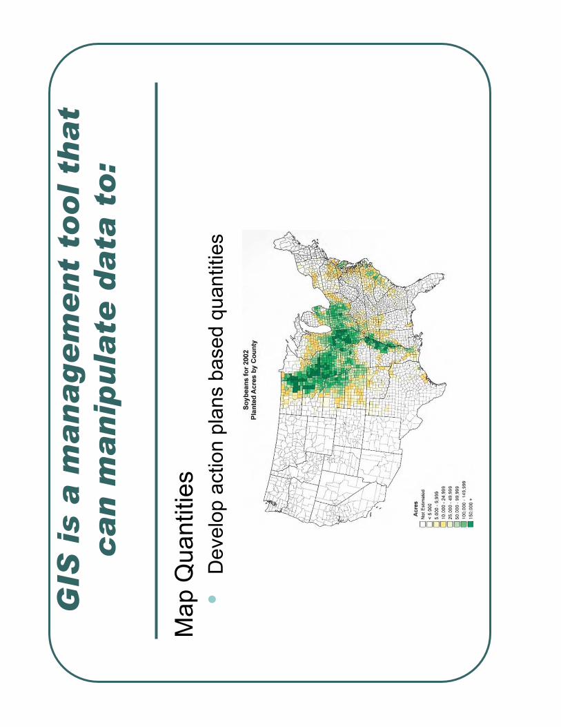
2. Map Quantities a. Develop action plans based quantities
3. Map Densities a. Visualize distribution of items across large areas
4. Find What’s Inside or Nearby a. Track trends b. Monitor data is nearby communities that impacts your data
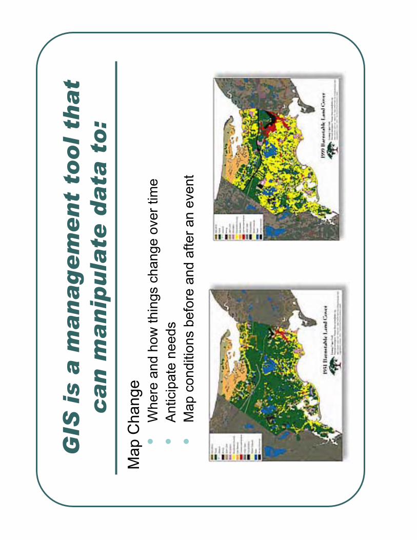
5. Map Change a. Where and how things change over time b. Anticipate needs

c. Map conditions before and after an event
(Information adapted from the ESRI website: http://www.gis.com/whatisgis/dowithgis.html)
Wrap Up Activity 7
Group led discussion
We have seen that GIS has the capability of being a great management tool for local
government, state and local agencies.
Can you envision some of the applications of this technology in our community?
What might be some of the jobs or careers that will utilize this technology? Can you identify
the possibilities right here in our community?
EVALUATION MODEL
Beginning of Next Day –Introductory GPS Quiz #3
EXTENSIONS
Extensions for Lesson 7 1. Invite to your school a representative of a local University that offers a GIS or
Geography major. Have them discuss the career opportunities that await an individual with the skills to operate GIS and GPS equipment.
2. Assign students to research sources of data and maps created using GIS technology. Have students share there finding s with the class.
Teacher Preparations for Lesson 8, 9, 10 1) Lesson Eight will require Adobe Acrobat Reader and computer access to the internet.
Be prepared to break students into workable groups with copies of the instructions and access to the internet.
2) Lesson Nine requires ArcExplorer version 9.1, a free program available on the internet. Follow the instructions in Appendix 1 to complete the download and instillation of the program.
3) Lesson Ten requires ArcView and ArcVoyager. Both of these programs are available for a fee from ESRI. You will not be able to complete Lesson Ten without these programs.

GIS
is a
ma
na
ge
me
nt
too
l th
at
ca
n m
an
ipu
late
da
ta t
o:
Ma
p t
he
ge
og
rap
hic
al lo
ca
tio
n o
f o
bje
cts
•U
se to fin
d a
location
•V
isualiz
e p
attern
s b
ased o
n the d
istr
ibution o
f fe
atu
res
Pow
erP
oin
t Lesson 7
GIS
is a
ma
na
ge
me
nt
too
l th
at
ca
n m
an
ipu
late
da
ta t
o:
Map Q
uantities
•D
eve
lop
actio
n p
lan
s b
ase
d q
ua
ntitie
s

GIS
is a
ma
na
ge
me
nt
too
l th
at
ca
n m
an
ipu
late
da
ta t
o:
Map D
ensitie
s
•V
isu
aliz
e d
istr
ibu
tio
n o
f ite
ms a
cro
ss la
rge
are
as

GIS
is a
ma
na
ge
me
nt
too
l th
at
ca
n m
an
ipu
late
da
ta t
o:
Fin
d W
hat’s Insid
e o
r N
earb
y
•T
rack tre
nds
•M
onitor
data
is n
earb
y c
om
munitie
s t
hat
impacts
your
data
GIS
is a
ma
na
ge
me
nt
too
l th
at
ca
n m
an
ipu
late
da
ta t
o:
Map C
hange
•W
here
and h
ow
thin
gs c
hange o
ver
tim
e
•A
nticip
ate
ne
ed
s
•M
ap c
onditio
ns b
efo
re a
nd a
fter
an e
vent

GIS
Map
pin
g -
Agri
cult
ure
Lesson #
7 G
IS S
am
ple
Map

GIS
Map
pin
g -
Fore
stry
Lesson #
7 G
IS S
am
ple
Map

Exploring Geographic Careers
at the ESRI Map Book Gallery
George Dailey
ESRI Education Programwww.esri.com/k-12
2004, ESRI, Inc. (Rev.1, 11/04)
Overview: This activity has students explore an online site filled with maps from
people in various walks of life, who are doing geographic research. It is intended tohelp expand their notions about the relevance of geography in everyday life and its
importance to educational and career pathways they might consider.
Time required: One class period.
Resources needed: Computer lab with Internet access, white board, writingsupplies.
Procedure:
1. As a pre-exploration activity, ask the students what they think geographers andpeople who work with geography do in the everyday world. What kinds of tasks
do they accomplish? List these on the board.
2. Let this run for several minutes or until the students seem complete in their
offerings. Don't be surprised if there are few comments.
3. As a small group or individual student activity, tell the students that they are
going to explore a Web site that will give them a more complete picture of
geography's role in numerous careers and tasks. The Web site is the ESRI Map
Book Gallery (www.esri.com/mapmuseum/index.html). This site displaysthe contents of the 2001-2004 map books that ESRI publishes each year. These
map books contain examples of output from geographic research from around
the world created by people and organizations tackling a wide range of
geographic tasks. Besides geography, students will see science, math,
technology, and communications in action.
4. Using a Web browser, direct the students
to the ESRI Map Book Gallery
www.esri.com/mapmuseum/index.html).
Ask each group or student to explore any
of the map books they choose.
5. The students task is to explore various
map images finding three that are
interesting to them.

6. As they find these, have them write down exactly
from which book and category each is. Also, have
them record:
Information on the topic being mapped
Map title Name of the organization
Their best estimate of what they think
the occupation of the person or people making
the map might be
Exploring geographic careers at the ESRI Map Book Gallery 2004, ESRI, Inc. (Rev. 1, 11/04)
2
Where the organization is located (e.g., Denmark)
San Diego/Baja California Border Region PlannedLand Use. San Diego Association of GovernmentsMost importantly, what interests them about
each map they select
7. Allow the students about 15-20 minutes for exploration as each of the four
volumes contains over 100 maps.
NOTE: If needed, take them on a tour of one of the maps in the Volume 16-18,exploring the viewer. If you wish, you can download another special viewer
plug-in from Lizard Tech. This is not necessary as the maps can be enlarged
without it. The maps in Volume 19 can be enlarged as simple Web images.
8. After the explorations, begin a class discussion of what was discovered. Allow
each group or a random selection of students to describe their favorites and why.
9. On the board, record at least the occupations the students have uncovered in
the investigation. While geographer may be in the listing that develops, it will be
clear that there are many, many occupations around the world where geographyis a critical component.
10.How does this list compare with the one they generated earlier? Use this
opportunity to re-emphasize that geography and geographic skills are key to
every one of the research projects they just explored.
11.If done as an individual student activity, consider having the students write a
short essay about the maps that interest them, if they have identified any new
career paths for themselves, and how they see geography fitting into them.
12. As a follow-on activity, direct the students to the “Careers in GIS” section of
GIS.com (www.gis.com/careers). Here they will be able to explore many more
aspects of the career possibilities ahead of them, and the importance of
geography in each. You can easily create more career lessons from the rich set
of resources available at this site.

Copyright © 2004 ESRI, Inc. www.esri.com/k-12
Using ArcExplorer™ Java™ Edition for Education
AEJEE is a stand-alone package of software that includes a Java Runtime Engine in the installation. AEJEE is a free tool designed for use particularly in education environments.
1. Check the system specifications a. Windows: Win98 or above, 100 MB hard drive space, Internet connection;
recommend Pentium III or faster processor, recommend more than 64 MB RAM b. Macintosh: MacOS 10.3 or above,100 MB hard drive space, Internet connection;
recommend G4 or faster processor; recommend more than 64 MB RAM
2. Download AEJEE from the Internet: www.esri.com/arcexplorer (click "download").
There are separate downloadable installers for Windows and for Macintosh. Please note that the downloads are large -- over 40 MB -- so be prudent in downloading. Use your file compression software to uncompress the downloaded installer, placing it in a folder where you can find it.
3. WINDOWS INSTALLATION:
a. Using Windows Explorer, navigate to the folder holding the uncompressed installation file,"install.exe".
b. Double-click the installer and follow the instructions. AEJEE defaults to install in C:\ESRI\AEJEE. If you change this folder, you will need to change the AEJEE project files before they can work. We recommend installing in the default directory.
4. MACINTOSH INSTALLATION:
a. Using Finder, navigate to the folder holding the uncompressed installation file "Install".
b. Double-click the installer and follow the instructions. AEJEE defaults to install in /ESRI/AEJEE. If you change this folder, you will need to change the AEJEE project files before they can work. We recommend installing in the default directory.
5. Getting Started with AEJEE a. Create an AEJEE Document Kit for yourself or the station(s). Print the AEJEE
"Getting Started" lessons, placing them in a binder. b. Introduce yourself to AEJEE by walking thru the lessons above. Look for more
lessons at www.esri.com/arclessons.
6. Introduce GIS to your students.
a. Show students what GIS is and how it is used in the real world using these sources: 1. http://www.gis.com. 2. http://www.esri.com/mapmuseum 3. http://www.gisday.com 4. http://www.geographynetwork.com5. http://www.esri.com/communityatlas
b. Take students through "Getting Started with AEJEE" lessons

Copyright © 2004 ESRI, Inc. Getting Started with AEJEE, Lesson 1 Page 1
Getting Started with ArcExplorer™ Java™ Edition for Education – Lesson 1
1. ArcExplorer Java Edition for Education (or "AEJEE") defaults to install in the "ESRI" folder at the root level of your hard drive. The "AEJEE" folder contains the AEJEE application and a "data" folder. By double-clicking the AEJEE icon, you can begin the application.
2. Once you have begun the application, the easiest way to explore what it can do is to open an existing file. Inside the /ESRI/AEJEE/data folder are several subfolders plus some files named like "2_us_hd.axl". These are "project" files. Start by choosing to open the file "2_us_hd.axl". This will open up a map about the US. (The "hd" in the name shows that it uses sample data from the hard drive, in contrast with projects containing "gn" for "Geography Network"; more about this later.) The "2_us_hd.axl" project explores data about farm acreage in the US.
3. The project opens with a map showing the 48 conterminous states, colored from green to grey. To the left of the map is a column containing several layers of data; the column is the "Table of Contents" (or "TOC"). The map at the right has been built using the layers in the TOC which have a black checkmark to the left of the name – "states" and "states: CropAcres97". Those layers with an empty checkbox are available for display in the map but are not currently turned on. The map opens with two layers on and five layers off.
4. You can turn layers on and off as you like, by clicking one time in the checkbox to the left of the layer name. An empty box means the layer will not show; a black check mark means the layer will show. Each time you make a change, the map re-draws, starting with the bottommost layer in the TOC first, on up to the topmost layer. Each layer has been set up in advance to show particular information with a specific symbol.

Copyright © 2004 ESRI, Inc. Getting Started with AEJEE, Lesson 1 Page 2

Copyright © 2004 ESRI, Inc. Getting Started with AEJEE, Lesson 1 Page 3
5. If you turn on the "rivers" layer, and have the "states" layer above it turned on also, you can see that parts of some rivers are also state borders. In this case, the black state border will display atop the blue river in the map, because the state layer is above the river layer in the TOC. In the TOC, right-click on "rivers", scroll down to "Move Layer", and choose "Up" to move the rivers layer up one layer in the TOC. Do it again to move the "rivers" layer above the "states" layer. Finish by moving the "states" layer back above the "rivers" layer.
6. Set your map so only the layer called "states: CropAcres97" is turned on. It has been set up to show each state in one of five categories, according to how many acres of cropland it had in 1997. The darkest looking states had the most (over 20 million acres), and the lightest state had the least. Do you know the name of the big southernmost dark green state?

Copyright © 2004 ESRI, Inc. Getting Started with AEJEE, Lesson 1 Page 4
7. What if you don’t know the name of the state? You can use the computer to find out. Above the map is a set of tools and menus. When you pause your mouse over a tool, a word or phrase called a "tooltip" appears, telling what the tool does. Look for the little circled "i" tool, which is the "Identify" tool. Click it. Click on the same big southernmost dark green state you named before. What shows up is an "Identify Results" window, providing a set of information about the state you clicked. In the left-hand column, you can see the name of the feature you selected, which should say "Texas". In the right-hand area, you can see many pieces of information about the state. In the right-hand column, scroll down to the bottom, to find "CROP_ACR97". This is the set of information being displayed in the map. In the TOC for your map, you should see that the number of acres for Texas is properly represented by a dark green color.
8. Each feature in the map is tied to a set of information about that feature. If you click with the identify tool on another state, you’ll find data about that state. Click on the southeasternmost state, and you should see information about Florida, including its crop acreage. Click on the northeasternmost and you’ll see information about Maine, including its crop acreage. In any given layer, each feature in that layer carries the same kind of information.
9. The same light-to-dark pattern is used for counties as well. By turning on the "counties: CropAcres97" layer and the "states" layer above it, you can see counties within the states, Looking at the pattern of counties across the states, you can see the areas that have a lot of farming (darker green) and those that have less (lighter green or grey). Can you name the states with lots of dark green counties?
10. Set only the layer "counties: CropAcres97" on. State boundaries have disappeared. Turn on the "states" layer. If you use the Identify tool when the "states" layer is on, AEJEE gives information about the state you click on. By turning off the "states" layer, and leaving on the "counties: CropAcres97" layer, you can now find information about one of the counties. AEJEE will identify features in whatever is the topmost layer being displayed. If you look at the info about some of the dark green counties, you can see that their info includes "STATE_NAME." In what states do you find the darkest green counties?
11. You can find out names of other features, such as rivers and lakes, by setting those layers as the topmost layer displayed and using the identify tool. What two rivers in Texas flow through the zone of Texas counties with the highest cropland?
12. The tools immediately to the left of the Identify tool are for panning and zooming. Again, pause the mouse over the tools to see what they do. Find and click the "Zoom to Full Extent" button; you’ll zoom out to the

Copyright © 2004 ESRI, Inc. Getting Started with AEJEE, Lesson 1 Page 5
extent of everything that is in the TOC. Which has more cropland – Alaska or Hawaii?
13. Use the "Zoom In" tool to zoom to the single state of your choice. (Use a "click-hold-drag diagonally" method to zoom to a specific area.) If you mess up, use the "Pan" tool to slide around, or the "Zoom to Full Extent" tool to start again. Return to a 48-state view when you’re done.
14. Click one time on the name of the "states" layer, to highlight the name. Click the "Find" tool. Since you highlighted the "states" layer, that layer is highlighted in the list of features you can find, but you may choose other features. For now, keep "states" highlighted and type "Iowa" (with a capital "I") in the "Value" box at the top. Click the "Find" button, and AEJEE will find Iowa and highlight it in yellow. Click "Zoom To" and AEJEE will move Iowa into the center of the map and zoom in.
15. We want to find which county in Iowa has the most cropland, but if you turn on the "counties: CropAcres97" layer, they look pretty similar. First, we need to select the counties of Iowa, which we can do with a query – asking the computer to highlight counties which meet a particular set of criteria.
16. In the TOC, click one time on the name of the layer "counties: CropAcres97" to highlight it. Click the "Query Builder" tool. Up comes the "Query Builder" window. This is where you can carefully build a set of criteria for AEJEE to apply. In the upper left corner, under "Select a Field", double-click "STATE_NAME", and notice that "STATE_NAME" is used to begin a statement, just above the "EXECUTE" button. In the upper center function pallet, click "=", and notice it gets added to the growing query statement above the "EXECUTE" button. In the upper right "Values" area, scroll down and double-click "Iowa". Now your statement should read "(STATE_NAME = 'Iowa')". Click "EXECUTE". In a couple of seconds, all the counties with a state name of Iowa will be highlighted ("selected") in the map of Iowa, and their attributes will appear at the bottom of the Query window. (How many counties are there in Iowa?)
Copyright © 2004 ESRI, Inc. Getting Started with AEJEE, Lesson 1 Page 6
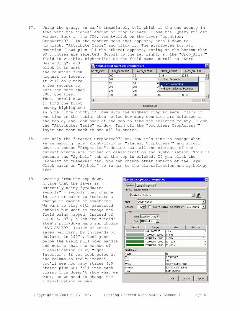
17. Using the query, we can’t immediately tell which is the one county in Iowa with the highest amount of crop acreage. Close the "Query Builder" window. Back in the TOC, right-click on the layer "counties: CropAcres97". In the context-menu that appears, scroll down to highlight "Attribute Table" and click it. The attributes for all counties (Iowa plus all the others) appears, noting at the bottom that 99 counties are selected. Scroll to the far right, so the "Crop_Acr97" field is visible. Right-click on the field name, scroll to "Sort Descending", and click it to sort the counties from highest to lowest. It will only take a few seconds to sort the more than 3000 counties. Then, scroll down to find the first county highlighted in blue – the county in Iowa with the highest crop acreage. Click it one time in the table, then notice how many counties are selected in the table, and look back at the map to find the selected county. Close the "Attributes Table" window. Turn off the "counties: CropAcres97" layer and zoom back to see all 50 states.
18. Set only the "states: CropAcres97" on. Now it’s time to change what we’re mapping here. Right-click on "states: CropAcres97" and scroll down to choose "Properties". Notice that all the elements of the current window are focused on classification and symbolization. This is because the "Symbols" tab at the top is clicked. If you click the "Labels" or "General" tab, you can change other aspects of the layer. Click again on "Symbols" to return to the classification and symbology area.
19. Looking from the top down, notice that the layer is currently using "graduated symbols" – symbols that change in size or color to indicate a change in amount of something. We want to stay with graduated symbols but want to change the field being mapped. Instead of "CROP_ACR97", click the "Field" item’s pull-down menu and choose "AVG_SALE97" (value of total sales per farm, by thousands of dollars, in 1997). Look just below the Field pull-down handle and notice that the method of classification is by "Equal Interval". If you look below at the column called "Records", you’ll see how many states (50 states plus DC) fall into each class. This doesn’t show what we want, so we need to change the classification scheme.

Copyright © 2004 ESRI, Inc. Getting Started with AEJEE, Lesson 1 Page 7
20. First, change the number of classes from 5 to 4, using the "Classes" pull-down menu, just below the "Field" menu. Notice that the number of records in each class has changed, since the divisions changed. But even this doesn’t give the best picture. Instead of "Equal Interval" classification, let’s use "Manual". Click the "Classified By" and select "Manual".
21. When you choose "Manual", a "Class Breaks and Histogram" window appears. The four colors show the range of values and the number of states within each value. The vertical bars represent the states. Move the mouse on top of the line separating color bands in the histogram, and notice that there is a point where the mouse arrow becomes a crosshair. By carefully clicking on the line separating color bands when the mouse arrow has become a crosshair, you can drag the "breakpoint" up or down to a new spot. As you drag, the break number will show the change. This method, however, can leave you with some breakpoints that are hard to use. Instead, let’s use the number boxes to the left of the histogram window to type in the breaks.
22. Click in the "Select Break" window and choose "-99.0". This is the lowest value of the 51, and you cannot change it. Neither can you change the highest value, "310.73". You can only change the intermediate breakpoints – the numbers at which you want to see a color change. Click in the "Select Break" window and choose the number closest to "310.73"; this is the number for which we will define a new breakpoint. Click in the "Current" window, erase the numbers visible, and type in "150.0" and press the Return key on your keyboard. Notice that the breakpoint changes in the histogram. Click in the "Select Break" window again and choose the number closest to "-99.0". Click in

Copyright © 2004 ESRI, Inc. Getting Started with AEJEE, Lesson 1 Page 8
the "Current" window, erase the numbers visible, and type in "50.0" and hit Return. Notice the lowest category jumps. Last, click in the "Select Break" window again and choose the number between 50 and 150. Click in the "Current" window, erase the numbers visible, and type in "100.0" and hit Return. At the bottom of the Histogram window, click the "OK" button.
23. We’re almost done with the map changes. Before we can apply the changes, we need to change the title of our layer. Click on the "General" tab at the top of the "states: CropAcres97 Properties" window. In the "Layer Name" box, change it to "states:CropValue97($K)". Then click "OK". Now, your map is different, showing the value produced per farm in thousands of dollars in 1997.
24. If you can’t quite see the title of each layer and you want to widen the TOC, move the mouse onto the middle of the line separating the TOC from the map. Click-hold-drag the line to the right a little bit, then let go. The map will redraw and the TOC will show more info.
25. To finish up, we want to clean up the display. Click on the "-" icons to collapse the legends for all layers except "states:CropValues97($K)" and make sure they are all off. With lots of space in the TOC, turn on the overview map by clicking "VIEW/Overview Map". Put a layer in the overview map by right-clicking "states" and choosing "Use in Overview Map". The shaded area shows the region in the main map.

Copyright © 2004 ESRI, Inc. Getting Started with AEJEE, Lesson 2 Page 1
Getting Started with ArcExplorer™ Java™ Edition for Education – Lesson 2
1. ArcExplorer Java Edition for Education (or "AEJEE") is able to work with data coming from local sources such as your LAN or hard drive and also from websites that serve geographic data through ArcIMS. Lesson 1 used only data installed with AEJEE on the hard drive. Lesson 2 will use data coming from the Geography Network. The difference in the source of the data is indicated by "hd" or "gn" letters in the project name.
2. Engage AEJEE and make sure you are connected live to the Internet. Navigate to the folder /ESRI/AEJEE/data and open the project "2_us_gn.axl".
3. The project opens with a set of data coming from the Geography Network (http://www.geographynetwork.com). At the top of the TOC, you’ll see "Census_TIGER2000", and the box with the black check mark will pulse in a green color while data are loading. The data can be used for free much like data from your hard drive, with a few key exceptions. You must be connected to the Internet to use it, and you don’t have as much opportunity to change the classification or symbolization, or do as much analytical work, but it often comes in as a pretty rich data set.
4. You’ll see a series of layers, all of which have a check-mark by the name, but some have a dark black check and others have a pale red check. Looking closely, you might even decide that some layers were duplicates. If you could inspect each layer, you’d find that each one
Copyright © 2004 ESRI, Inc. Getting Started with AEJEE, Lesson 2 Page 2
is in fact turned on, but each is set to display only when the map is zoomed to a certain scale. The reason for having multiple layers is to set it up so that different data are visible at different times. These are "scale-sensitive data layers."
5. You can see the scale sensitivity by zooming from 50 states to your multi-state region, then to your state, then inside the state, then down to your neighborhood. At different scales, different layers become visible and usable; this is controlled within the properties for each individual layer. Each time you zoom in or out, the software reaches across the internet to re-access the data. Zoom to your state so you can see the full state but set it to be as large as possible in your map. How many layers have black check marks?
6. Zoom in to your neighborhood and notice that features magically appear as you get closer. The scale of the map (such as 1:100,000) shows as a ratio below the map. When you are at a scale closer than 1:50,000 (such as 1:40,000), click in the TOC one time right on the name of the "Streets" layer with a black check mark, thus highlighting that layer. Click on the "Identify" tool, then, with the tip of the mouse arrow, click on a street. The software should reach back across the Internet, find information about the street, and in a few seconds present it to you in an "Identify Results" window. It may be hard to read everything, so make the window about an inch wider so you can see the full names in the "Field" column. Look down the list for "TGR.TGR_ROADS_FENAME", which will give the "feature name". All the other fields carry additional info about the particular road segment on which you clicked.
7. Try zooming in to a scale closer than 1:15,000 (such as 1:14,000). What happens this close that did not happen when zoomed farther out?
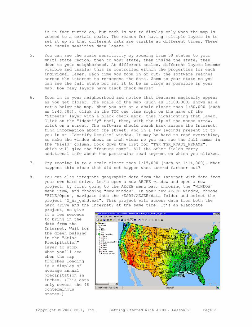
8. You can also integrate geographic data from the Internet with data from your own hard drive. Let’s open a new AEJEE window and open a new project, by first going to the AEJEE menu bar, choosing the "WINDOW" menu item, and choosing "New Window". In your new AEJEE window, choose "FILE/Open", navigate into the /ESRI/AEJEE/data folder and select the project "2_us_gnhd.axl". This project will access data from both the hard drive and the Internet, at the same time. It’s an elaborate project, so give it a few seconds to bring in the data from the Internet. Wait for the green pulsing in the "Atlas Precipitation"layer to stop. What you’ll see when the map finishes loading is a display of average annual precipitation in inches. (This data only covers the 48 conterminousstates.)
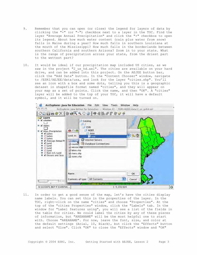
Copyright © 2004 ESRI, Inc. Getting Started with AEJEE, Lesson 2 Page 3
9. Remember that you can open (or close) the legend for layers of data by clicking the "+" (or "-") checkbox next to a layer in the TOC. Find the layer "Average Annual Precipitation" and click the "+" checkbox to open its legend. About how much water content (rain plus water from snow) falls in Maine during a year? How much falls in southern Louisiana at the mouth of the Mississippi? How much falls in the borderlands between southern California and southern Arizona? Zoom in to your state. What is the range of precipitation across your state, from the driest part to the wettest part?
10. It would be ideal if our precipitation map included US cities, as we saw in the project "2_us_hd.axl". The cities are available on your hard drive, and can be added into this project. On the AEJEE button bar, click the "Add Data" button. In the "Content Chooser" window, navigate to /ESRI/AEJEE/data/usa, and look for the layer "cities.shp". You’ll see an icon with a box and some dots, telling you this is a geographic dataset in shapefile format named "cities", and they will appear on your map as a set of points. Click the name, and then "OK". A "cities" layer will be added to the top of your TOC, it will have a default symbol, and it will be turned on.
11. In order to get a good sense of the map, let’s have the cities display name labels. You can set this in the properties of the layer. In the TOC, right-click on the name "cities" and choose "Properties". At the top of the "cities Properties" window, click the "Labels" tab. In the window for "Label features using", you will see a list of the fields in the table for cities. We could label the cities by any of these pieces of information, but "AREANAME" will be the most helpful one to start with. Choose "AREANAME". For now, leave the font, size, and color at the default settings (Arial, 10, Black), but click the "Effects" button and select "Glow". Click "OK" to close the "Effects" window and "OK"

Copyright © 2004 ESRI, Inc. Getting Started with AEJEE, Lesson 2 Page 4
again to set the labels to display. You’ll return to the map and have city names displayed with a yellow glow around the city name. (If you are viewing cities atop a yellowish precipitation zone, it may be hard to see the glow.)
12. In the TOC, right-click on the name "states" and scroll down to choose "Zoom to layer". You’ll jump out to see all 50 states, and the cities and counties layers will make your map messy. Turn off the cities and counties, then zoom in to see the 48 states. Using the layer properties for "states", set the labels to display "STATE_ABBR", and turn on the "glow" effect. What is the two-letter abbreviation for the northwestern state with the highest annual precipitation, and how much rain do they get? Which state has a greater range of precipitation zones, California or Texas?
13. Zoom in to Wyoming. Yellowstone park is in Wyoming where it meets Montana and Idaho. Is it relatively dry or wet there? What might be different in the Yellowstone region compared with the eastern parts of Wyoming? What would you want to add to this map in order to verify your answer? Let’s add some more data, but this time from across the Internet, from the Geography Network. First, let’s clean up your map. Collapse the "Atlas_Precipitation" legend by clicking the "-" icon, then turn off the "Atlas_Precipitation" layer, leaving your map showing an empty box labeled "WY".
14. Click the "Add Data" button. In the Content Chooser window, click the pull-down "Look in" item and select "Internet Servers". Double-click "Add Internet Server." In the "ArcIMS4 Connection" window, set the URL to http://www.geographynetwork.com, and select "Connect to ArcIMS4 Services". Click OK. In the Content Chooser window will appear a set

Copyright © 2004 ESRI, Inc. Getting Started with AEJEE, Lesson 2 Page 5
of data options available from the Geography Network. Scroll to find "ESRI_Relief" and choose it, then click "OK." Inside, you’ll find another icon labeled "ESRI_Relief". Choose this one and click "OK". A new layer called "ESRI_Relief" will be added to the bottom of your map. When it appears, you’ll see a grey-shaded display, showing mountains, hills, and plains. Was your answer to the Yellowstone question correct? Turn the "Atlas_Precipitation" layer back on to see. (You can turn the layers off and on pretty quickly if you don’t change the scale.)
15. Are you ready to save this project? Let's save the project under a new name, but in the same place as the other projects. In the AEJEE menu bar, choose "FILE/SaveAs". Navigate to /ESRI/AEJEE/data and name this project "2_us_gnhd_plus.axl", then click "Save". Just like in your other software packages, you can come back later and re-open this project. It doesn’t save the data with the project, it only saves a "recipe" for where to find each data set, how they are classified and symbolized, and the area to be displayed in the map.

Copyright © 2004 ESRI, Inc. Getting Started with AEJEE, Lesson 3 Page 1
Getting Started with ArcExplorer™ Java™ Edition for Education – Lesson 3
1. ArcExplorer Java Edition for Education (or "AEJEE") is able to work with data coming from local sources such as your LAN or hard drive and also from websites that serve geographic data through ArcIMS. Lesson 1 used only data installed with AEJEE on the hard drive. Lesson 2 used data coming from both the hard drive and the Geography Network. Both lessons used data about the US in map windows that presented the data in a "projected" format. Lesson 3 will focus on map projections within AEJEE.
2. Engage AEJEE and navigate to the folder/ESRI/AEJEE/data,then open the project "1_world_hd.axl".AEJEE will display the world in a rectangular fashion, centered on the Prime Meridian (0 degrees longitude), with all the world visible at once. Each of the blue boxes in the background,representing ocean regions 30 degrees on a side, is the same size.
3. Let’s open a new window with a different display. In the AEJEE menu bar, choose"WINDOW/NewWindow". A new, empty display appears on top of your first window. Slide the new window just a little bit so that you can see there are two different AEJEE windows. In this second window, open the project "1_world_hd2.axl".
4. The two maps use exactly the same data, but different projections. The second window shows the world as a sphere, or rather a flat representation of a sphere. The data in the TOC are stored in a "decimal degree coordinate system" and the map space has been "projected" to look like what we know as a globe. Projections, coordinate systems, and datums are somewhat complicated, but they are
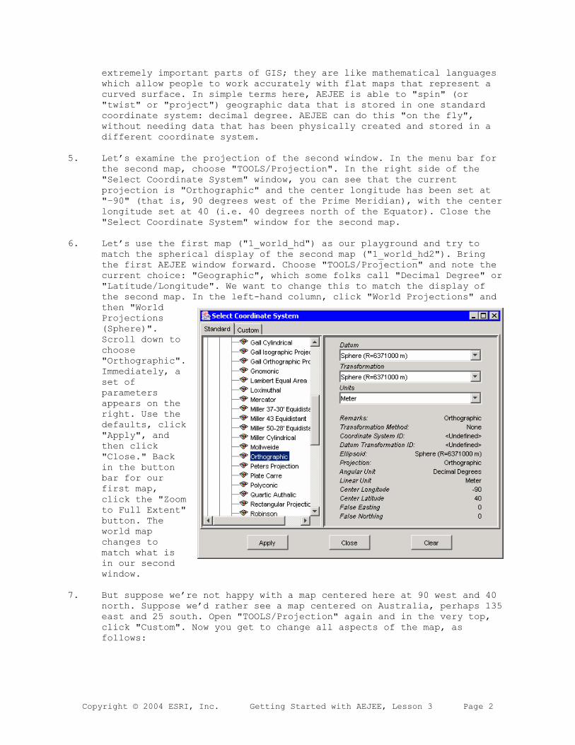
Copyright © 2004 ESRI, Inc. Getting Started with AEJEE, Lesson 3 Page 2
extremely important parts of GIS; they are like mathematical languages which allow people to work accurately with flat maps that represent a curved surface. In simple terms here, AEJEE is able to "spin" (or "twist" or "project") geographic data that is stored in one standard coordinate system: decimal degree. AEJEE can do this "on the fly", without needing data that has been physically created and stored in a different coordinate system.
5. Let’s examine the projection of the second window. In the menu bar for the second map, choose "TOOLS/Projection". In the right side of the "Select Coordinate System" window, you can see that the current projection is "Orthographic" and the center longitude has been set at "–90" (that is, 90 degrees west of the Prime Meridian), with the center longitude set at 40 (i.e. 40 degrees north of the Equator). Close the "Select Coordinate System" window for the second map.
6. Let’s use the first map ("1_world_hd") as our playground and try to match the spherical display of the second map ("1_world_hd2"). Bring the first AEJEE window forward. Choose "TOOLS/Projection" and note the current choice: "Geographic", which some folks call "Decimal Degree" or "Latitude/Longitude". We want to change this to match the display of the second map. In the left-hand column, click "World Projections" and then "World Projections(Sphere)".Scroll down to choose"Orthographic".Immediately, a set of parametersappears on the right. Use the defaults, click "Apply", and then click "Close." Back in the button bar for our first map, click the "Zoom to Full Extent" button. The world map changes to match what is in our second window.
7. But suppose we’re not happy with a map centered here at 90 west and 40 north. Suppose we’d rather see a map centered on Australia, perhaps 135 east and 25 south. Open "TOOLS/Projection" again and in the very top, click "Custom". Now you get to change all aspects of the map, as follows:

Copyright © 2004 ESRI, Inc. Getting Started with AEJEE, Lesson 3 Page 3
a. Projection: Orthographic b. Datum: WGS84 c. Angular Unit: Decimal Degrees d. Linear Unit: This means how you want to measure distances, so
let’s choose "Int.Mile" e. Center Longitude: 135.0 f. Center Latitude: -25.0 g. False Easting: 0.0 h. False Northing: 0.0
Then click "Apply" and "Close", and "Zoom to Full Extent"
8. Using this method, you can set AEJEE to display the world centered on any coordinate, including the poles.
9. You can use the Projection window to select a wide assortment of standard projections, or customize the display infinitely. Are you looking for a nice equal area map of the world, showing the world’s land masses at their proper size? Choose "Standard", "World Projections", "World Projections (Sphere)", and "Eckert IV". Apply the changes and close the Projections window, then click the "Zoom to Full Extent" button to adjust the map.
10. What if you want to see the same "Eckert IV" projection but showing the Pacific Ocean as an unbroken body? Again, go into the Custom settings, as follows:
a. Projection: Eckert IV b. Datum: WGS84 c. Angular Unit: Decimal Degrees d. Linear Unit: "Int.Mile" e. Center Longitude: 150.0 f. False Easting: 0.0 g. False Northing: 0.0
Then click "Apply" and "Close", and "Zoom to Full Extent"
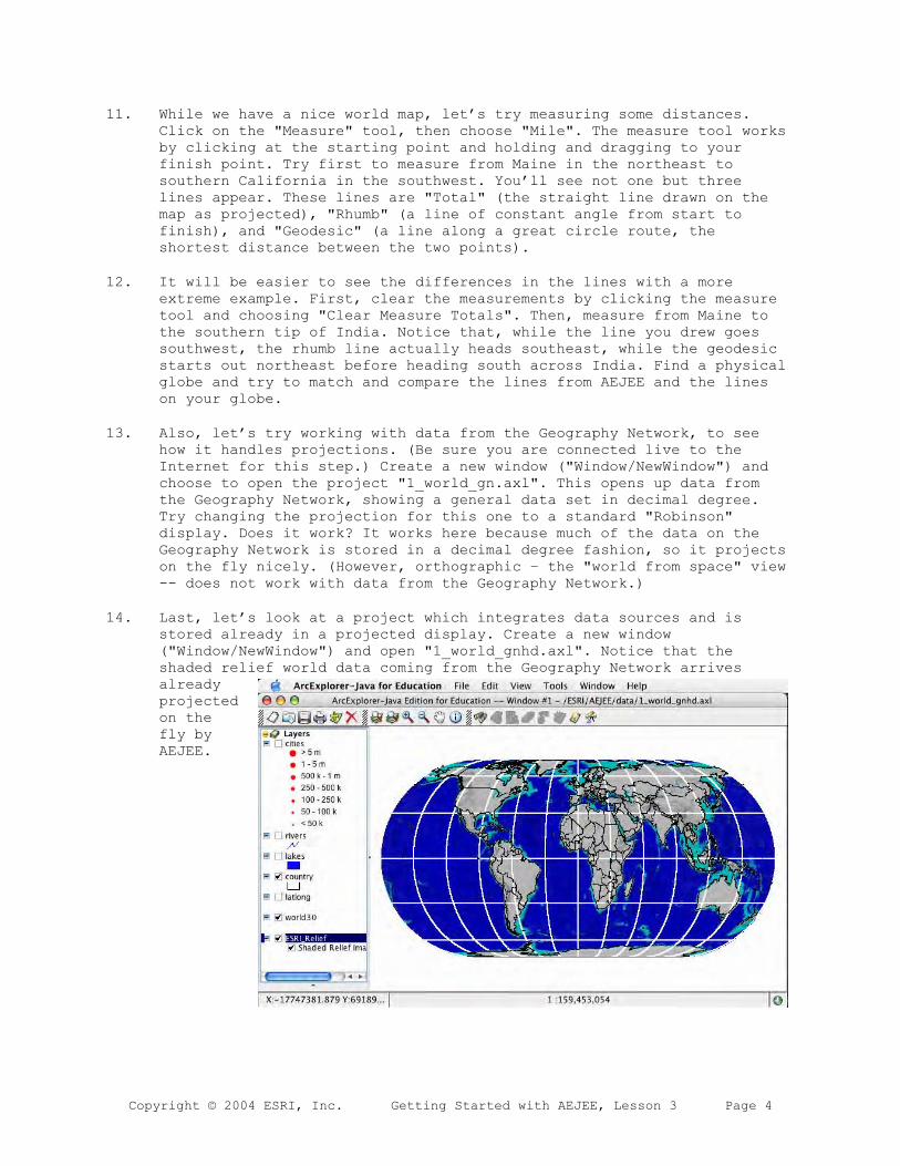
Copyright © 2004 ESRI, Inc. Getting Started with AEJEE, Lesson 3 Page 4
11. While we have a nice world map, let’s try measuring some distances. Click on the "Measure" tool, then choose "Mile". The measure tool works by clicking at the starting point and holding and dragging to your finish point. Try first to measure from Maine in the northeast to southern California in the southwest. You’ll see not one but three lines appear. These lines are "Total" (the straight line drawn on the map as projected), "Rhumb" (a line of constant angle from start to finish), and "Geodesic" (a line along a great circle route, the shortest distance between the two points).
12. It will be easier to see the differences in the lines with a more extreme example. First, clear the measurements by clicking the measure tool and choosing "Clear Measure Totals". Then, measure from Maine to the southern tip of India. Notice that, while the line you drew goes southwest, the rhumb line actually heads southeast, while the geodesic starts out northeast before heading south across India. Find a physical globe and try to match and compare the lines from AEJEE and the lines on your globe.
13. Also, let’s try working with data from the Geography Network, to see how it handles projections. (Be sure you are connected live to the Internet for this step.) Create a new window ("Window/NewWindow") and choose to open the project "1_world_gn.axl". This opens up data from the Geography Network, showing a general data set in decimal degree. Try changing the projection for this one to a standard "Robinson" display. Does it work? It works here because much of the data on the Geography Network is stored in a decimal degree fashion, so it projects on the fly nicely. (However, orthographic – the "world from space" view -- does not work with data from the Geography Network.)
14. Last, let’s look at a project which integrates data sources and is stored already in a projected display. Create a new window ("Window/NewWindow") and open "1_world_gnhd.axl". Notice that the shaded relief world data coming from the Geography Network arrives alreadyprojectedon the fly by AEJEE.

Copyright © 2004 ESRI, Inc. Getting Started with AEJEE, Lesson 4 Page 1
Getting Started with ArcExplorer™ Java™ Edition for Education – Lesson 4
1. ArcExplorer Java Edition for Education (or "AEJEE") is able to work with data about specific geographic features coming from local sources such as your LAN or hard drive and also from websites that serve geographic data through ArcIMS. Lesson 1 used only data installed with AEJEE on the hard drive. Lesson 2 used data coming from both the hard drive and the Geography Network. Lesson 3 focused on map projections within AEJEE. Lesson 4 will add to the work on projections by integrating image data with shapefiles and adding point data from XY tables.
2. Engage AEJEE and navigate to the folder /ESRI/AEJEE/data, then open the project "3_dc_hd.axl". AEJEE will display the region around Washington DC using a satellite image. The image is a "false color" display, in which healthy vegetation shows up as red and human structures such as buildings or roads appear bluish. The image is stored in a format known as "Universal Transverse Mercator", using a datum of "North America 1983", and the specific zone is "18". These elements can be abbreviated as "UTM 18, NAD83".
3. When you wander your mouse around the display, you’ll see in the very bottom of the AEJEE window a pair of very large numbers. These numbers show the location in meters away from the standard beginning point of UTM 18 NAD83. (The size of the numbers is one indication that this is

Copyright © 2004 ESRI, Inc. Getting Started with AEJEE, Lesson 4 Page 2
not displayed in "decimal degree" space, since decimal degree numbers only go from a high of 180 to a low of –180.)
4. Draped on top of the image are some shapefiles that came from the ESRI TIGER Data website (www.esri.com/tiger), which is a place where GIS users can download data about any county in the U.S. The data comes originally from the U.S. Census Bureau, and the names look a little unusual here. Every county (or equivalent) in the U.S. has a specific 5-digit code, and Washington DC is known as "11001". Let’s start by giving those layers more understandable names.
5. Find the layer "tgr11001wat", which has a blue box symbol. Right-click on the name "tgr11001wat", choose "Rename", and change the name to "waters", then hit the "Return" or "Enter" key to complete the change. In the same manner, change the following layer names:
a. "tgr11001lkh" to "streams" b. "tgr11001cty00" to "DC boundary" c. "tgr11001lka" to "roads"
6. Save your project in the same space as the other projects, but give it a new name, like "3_dc_hd2.axl".
7. Back in AEJEE, zoom in to the bluish area that is the heart of Washington DC, just north of the junction of two main rivers – the Potomac and the Anacostia. (Can you remember how to identify the rivers?) Zoom to a scale of about 1:30,000.
8. The map is fascinating, but we would like to add some point data for interesting sites, gathered with a global positioning system (GPS). First we need to create a data table to bring into AEJEE. Open up a simple text editor, such as NotePad (PC) or TextEdit (Mac). Create a document that looks exactly like this:
site,lat,long,name1,38.889,-77.035,Washington Monument 2,38.889,-77.050,Lincoln Memorial 3,38.898,-77.036,White House 4,38.889,-77.009,Capitol
Make sure you have only these five lines, and no extra spaces or characters that are not shown above. (Notice the latitudes are identical except for the White House, and the longitudes are negative.) Save this as a simple text file called "dcgps.txt" in the folder /ESRI/AEJEE/data/washdc. Exit your text editor and return to AEJEE.
9. We want to see on the map the GPS points that we just created with the coordinates above. AEJEE cannot display simple text files, but it can read such text files and create a regular shapefile. Choose "VIEW/AddEventTheme". Navigate to where you stored the text file. Highlight "dcgps.txt" and click "Open". AEJEE will tell you to select the X and Y fields; the "X" should be "longitude" or "long", and the "Y" should be "latitude" or "lat". AEJEE is going to create a shapefile in the "storage directory", which should be /ESRI/AEJEE/data/washdc. You can also pre-select what symbol you want AEJEE to use in displaying these points on your map. Try a star colored black and sized 18 points. Click OK.

Copyright © 2004 ESRI, Inc. Getting Started with AEJEE, Lesson 4 Page 3
AEJEE will create three new files in your "washdc" folder called "dcgps.shp", "dcgps.dbf", and "dcgps.shx"; together, these files constitute a shapefile called "dcgps" – the one now added to your map display! Because the map window is already projected, and the other feature data (such as roads and streams) is in decimal degree, the GPS data can integrate well with these layers. Use the layer properties for "dcgps" to set the label as "Name"; it may also help to set the label placement at the "12 o’clock" position.
10. Let’s select the point that is the White House. Click one time on the name of the "dcgps" layer, to highlight the layer. Click on the "Select Features" tool and choose "Rectangle". Click and drag a box encompassing the star symbol for the White House. A new dot appears, yellow, indicating it is selected. Now, click on the "Buffer" tool. Choose as a distance 1 mile, and click "OK". Around the White House will appear a shaded circle with a radius of 1 mile. Which of the three other features is not within a mile of the White House?

Copyright © 2004 ESRI, Inc. Getting Started with AEJEE, Lesson 4 Page 4
11. Erase the 1-mile buffer by clicking the "Clear All Selection" button. Use the Select tool to select the White House again. Click on the "Buffer" tool and choose as a distance 0.5 miles, and ask AEJEE to select features from the layer "Roads", then click "OK". Turn on the roads. The yellow road segments are all within a half-mile of the White House.

Copyright © 2004 ESRI, Inc. Getting Started with AEJEE, Lesson 5 Page 1
Getting Started with ArcExplorer™ Java™ Edition for Education – Lesson 5
1. ArcExplorer Java Edition for Education (or "AEJEE") is able to work with nicely with data from local sources and the Internet. Lessons 1-4 provided a basic introduction to these capacities. Lesson 5 focuses on sharing projects between computers and working with georegistration data for images.
Transportable Projects and AEJEE
2. AEJEE is able to save and open "projects" -- combinations of data presented in a particular fashion. Saving projects allows you to work on them again and again, and also to share them with others. But the project file (such as "3_dc_hd.axl") is simply an ASCII textfile recipe file, showing AEJEE where to find data and how to display it. In order for a project to work properly, the prescribed data sets need to be available in the prescribed location. Let's look at an example.
3. Open up either WordPad for Windows or TextEdit for Macintosh. Choose FILE/OPEN and navigate to the folder /ESRI/AEJEE/data, and select the file "1_world_hd.axl".

Copyright © 2004 ESRI, Inc. Getting Started with AEJEE, Lesson 5 Page 2
4. You can see the document lists aspects of the project in a format that looks like the source code for an HTML file. In fact, ArcXML is very much like HTML. Look after the big long paragraphs for the section from "<FOLDERS>" to "</FOLDERS>":
<FOLDERS> <FOLDER name="ws-0" type="shapefile"> <ATTRIBUTE name="directory" value="/ESRI/AEJEE/data/world"/> </FOLDER> </FOLDERS>
This shows that all the data in this project are stored in one folder, and shows the path starting from the root level of the hard drive. If you want to change the location of the folder, all you need to do is go in to the project and change this line, then re-save the project file.
5. When you save an AEJEE project on a Macintosh, this is how the data get stored. Both Macintosh and Windows versions of AEJEE can read this project just fine. However, if you re-save the above project on a Windows computer, it stores the data like this:
<FOLDERS> <FOLDER name="ws-0" type="shapefile"> <ATTRIBUTE name="directory" value="C:\ESRI\AEJEE\data\world"/> </FOLDER> </FOLDERS>
It may not look very different, but close inspection will reveal two key differences in the "value" portion. First, the hard drive has a drive letter and colon. Second, the PC saves with backslashes instead of forward slashes. These changes are enough to prevent Macintosh computers from reading the PC projects. But you can make them readable by both versions. Just open up the project, remove the "C:" references, and change the "\" characters to "/", then re-save.
GEO-REGISTERED IMAGES and AEJEE
6. The project "3_dc_hd.axl" engaged an image from the hard drive. The image has been "geographically registered" -- it knows the portion of the earth that it represents. The image itself is several megabytes in size, but it is the presence of two little files that provide the spatial intelligence. Navigate into the folder /ESRI/AEJEE/data/washdc and look for the files "wash.tif" (the big image file) plus "wash.tfw" (a world file, showing the coordinates for the image) and "wash.prj" (a projection file, showing the projection in which the image resides).
7. As you saw in the earlier lessons, AEJEE can project decimal degree features (points, lines, polygons) to match up with images. But it needs to have these two files in place in order to reference the image accurately. AEJEE cannot create the world files for images, nor the PRJ files -- you need full GIS software to do this. ArcView is an example of a GIS software package that can do this.

Copyright © 2004 ESRI, Inc. Getting Started with AEJEE, Lesson 5 Page 3
8. ArcView 3 and ArcView 9 can use images with world files; most images available for use in GIS packages contain a world file. World files are listed as "TFW" for "TIF" images, "JGW" for "JPG" images, "SDW" for "SID" images, and so forth. The world file is designed the same in each case, and AEJEE can use these world files.
9. ArcView 3 does not pay significant attention to PRJ files for images. ArcView 9 is able to write out projection information for images, but it creates the file in a format that isn't quite right for AEJEE. Once again, you can use a text editor to change the data presented by ArcView 9 so that it is more useful for AEJEE.
a. In AV9, engage the "Define Projection" toolbox. Input the image, choose the coordinate system, and click "OK". The toolbox will create a ".XML" file. Exit AV9.
b. Open the ".XML" file with TextEdit (Mac) or WordPad or NotePad (PC). Look halfway down for the section of text immediately following the path to the image and name:
c. Omit all the text leading up to "PROJCS" and following the double bracket after "UNIT"
d. Change all the ' marks to " marks. Then save the file as the .PRJ file (in this case, "wash.prj"), in the same folder with the image. Now AEJEE can match features with the images!

Appendix Two
Internet Resources
GPS Information Links
Links to General GPS Information
http://www.trimble.com/gps/
http://www.e-trimblegps.com/gps101.htm
Advanced GPS Equipment and Training
www.trimble.com
GPS GeoCaching Website
www.geocaching.com
GIS Sample Maps
http://www.usda.gov/nass/aggraphs/cropmap.htm
GIS Software Downloads
For Downloading ArcExplorer Version 9.1
http://www.esri.com/software/arcexplorer/index.html
4H GIS Curriculum Project (Downloadable guides)
Project books and guides for use on ArcExplorer Version 9.1
http://lal.cas.psu.edu/Research/edTraining/4h_GISprojectBooks.htm

GIS Lesson Plans
Lesson plans for various levels of GIS Applications
http://www.esri.com/industries/k-12/education/lessons.html
GIS Data Sites
Pennsylvania Spatial Data Access Clearinghouse – GIS Data for advanced applications
http://www.pasda.psu.edu/