Government Spending and Budget Deficits in the …homepage.ntu.edu.tw/~kslin/macro2009/Roubini and...

http://www.jstor.org

Government Spending and Budget Deficits in the Industrial CountriesAuthor(s): Nouriel Roubini, Jeffrey Sachs, Seppo Honkapohja, Daniel CohenSource: Economic Policy, Vol. 4, No. 8 (Apr., 1989), pp. 100-132Published by: Blackwell Publishing on behalf of the Centre for Economic Policy Research,Center for Economic Studies, and the Maison des Sciences de l'HommeStable URL: http://www.jstor.org/stable/1344465Accessed: 07/09/2008 03:38

Your use of the JSTOR archive indicates your acceptance of JSTOR's Terms and Conditions of Use, available at

http://www.jstor.org/page/info/about/policies/terms.jsp. JSTOR's Terms and Conditions of Use provides, in part, that unless

you have obtained prior permission, you may not download an entire issue of a journal or multiple copies of articles, and you

may use content in the JSTOR archive only for your personal, non-commercial use.

Please contact the publisher regarding any further use of this work. Publisher contact information may be obtained at

http://www.jstor.org/action/showPublisher?publisherCode=black.

Each copy of any part of a JSTOR transmission must contain the same copyright notice that appears on the screen or printed

page of such transmission.

JSTOR is a not-for-profit organization founded in 1995 to build trusted digital archives for scholarship. We work with the

scholarly community to preserve their work and the materials they rely upon, and to build a common research platform that

promotes the discovery and use of these resources. For more information about JSTOR, please contact [email protected].

http://www.jstor.org/stable/1344465?origin=JSTOR-pdf

http://www.jstor.org/page/info/about/policies/terms.jsp

http://www.jstor.org/action/showPublisher?publisherCode=black

Economic Policy April 1989 Printed in Great Britain

Fiscal policy Nouriel Roubini and Jeffrey Sachs

Summary

This paper examines the evolution of the size of government and of budget deficits in OECD economies. We highlight the rapid increase in government spending in the 1970s, the sharp rise in budget deficits and public debt after 1973, and the reversal in these trends in the 1980s.

The increase in the size of government was associated in part with the slowdown in growth after 1973, but also reflected gradual adjustment of the ratio of spending to output towards a long-run target which depends on political and institutional characteristics of the economy-the political orientation of the government, the degree of wage indexation, and the degree of stability of the political system.

Such factors also explain the size of budget deficits. When faced with an adverse shock, subsequent deficit reduction requires a measure of political consensus. We note that such consensus is hard to achieve in multi-party coalitions. In consequence, countries with such a political structure tended to experience much more rapid increases in their debt-GNP ratios.

Government spending and budget deficits in the industrial countries Nouriel Roubini and Jeffrey Sachs Yale University, Harvard University and NBER

1. Introduction This paper takes a broad look at the trends in government spending, taxation, and budget deficits in the OECD countries since the mid-1960s. It is directed at some important puzzles in the political economy of the industrial countries. The first puzzle is evident in Table 1. Throughout the past half century, there has been a steady increase in the share of government spending, G, in total national product, Y. What is notable, however, is the sharp rate of increase in G/Y beginning in the mid- 1960s. During the period 1973-82 (which we focus on for reasons discussed below), the share of government experienced its most rapid jump for any subperiod during the past 50 years. After 1982, government spending as a share of GNP has stabilized, and in some countries has even fallen.

Our first question, then, is how to account for the sharp rise in the share of government after the mid-1960s; the very rapid increase between 1973 and 1982; and the halt to a rising government share during the most recent years. Our analysis is necessarily broad-brushed and provisional, but it does point to some of the important underlying trend factors, as well as cyclical factors, behind the rise in the government share.

The second puzzle that we examine is the behaviour of government budget deficits and the public debt. Up until 1973, government deficits were sufficiently low in most countries to lead to a falling ratio of net public debt to GNP, which we denote as D/Y, and which is illustrated in Table 2.1 This is in line with Robert Barro's prediction of a falling

The authors would like to thank members of the Economic Policy panel, the two discussants and the editors for very helpful remarks.

Throughout the paper, D will represent the net debt of the public sector (liabilities minus financial assets), as calculated by the OECD. These data are not published and were obtained directly from the OECD.

Fiscal policy 101

Table 1. Public expenditure in selected OECD countries (% of GDP)

Year 1938 1950 1965 1973 1982 1985

France 21.8 27.6 38.4 38.5 51.1 52.4 Germany 42.4 30.4 36.6 41.5 49.4 47.2 Japan 30.3 19.8 19.0 22.4 33.7 32.7 Netherlands 21.7 26.8 38.7 45.8 61.6 60.2 UK 28.8 34.2 36.1 40.6 48.2 47.7 US 18.5 22.5 27.4 36.6 30.5 36.7 Italy 29.2 30.3 34.3 37.8 47.6 50.8

Sources: Lybeck and Henreckson (1988) (page 189) for 1938, 1950, 1985 figures. OECD Economic Outlook for 1973 and 1965 figures.

Table 2. Net debt as percentage of GDP

Year 1960 1973 1986

US 45.0 23.0 29.1 Germany -13.2 -6.7 22.1 France 29.1 8.3 18.2 UK 128.2 57.9 46.7 Italy 26.6t 45.1 84.9 Canada 21.8 2.6 33.7 Belgium 83.3 50.9 113.3 Finland -5.0* -10.7 -0.4 Austria 19.4* 17.5 47.7 Netherlands 28.9* 21.0 46.0 Sweden -24.0* -31.1 14.5 Norway 2.5* -1.4 -24.4 Japan -5.6t -6.1 26.3 Denmark -2.8* -12.2 28.5 Ireland 35.7* 32.0 108.2

* 1970 figure. t 1964 figure. 1 1965 figure. Source: OECD data.

debt-GNP ratio during periods of peacetime.2 But after 1973, the trend was reversed: almost every OECD economy experienced a significant rise in the debt-GNP ratio in the years 1973-85.

l I 2 Robert Barro has shown that the same phenomenon is true over a span of roughly 200 years

in both the US and the UK. In both cases, the public debt to GNP ratio usually fell during peacetime, and jumped during wartime. Barro has argued that this pattern reflects the application of optimal tax smoothing by the fiscal authorities. For details for the US, see Barro (1979), and for the UK, see Barro (1987).

Nouriel Roubini and Jeffrey Sachs

Part of the explanation for the rising debt ratio is simply the effect of the cyclical downturn in the OECD economies after 1973. But we suggest that a richer pattern is also evident, linking the size of the budget deficits to the political structure of the government. Weak and divided governments (as evidenced by the expected tenure in office, and by the number of political parties that share power in the governing coalition) have been less effective in reducing the budget deficit than have stable and majority-party governments.

One of our main themes is that the year 1973 marked a watershed for the OECD economies. That year was the end, at least for the next 15 years, of the high and noninflationary growth enjoyed by the industrial world in the 1950s and 1960s. Almost every industrialized country experienced a significant slowdown in average growth after 1973, together with a rise in unemployment rates and higher inflation. The high inflation began to abate in the early 1980s, but the slowdown in growth, and the higher unemployment in Europe, has proved to be more persistent. The reasons for the growth slowdown and rise in unemployment are still a matter of debate, but it seems clear that adverse supply shocks have played a significant role. All of the OECD economies experienced a steep decline in total factor productivity growth beginning in the early 1970s, and almost all suffered a terms-of-trade deterioration following the oil shocks of 1973 and 1979.3

These supply shocks posed a multi-faceted adjustment problem of profound economic and political consequence in the industrial countries. After 1973 real incomes in the aggregate could not grow as fast as they did before 1973. In a smoothly working economic and political system, this fact would prompt two important adjustments: a slower growth in real wages, in order to preserve full employment; and a slower increase in real government spending, in order to maintain a desirable balance between expenditures on private and public goods.

Actual adjustments were far from smooth. We now know from extensive analysis that real wages did not smoothly adjust to maintain a balance between labour costs and the marginal productivity of labour at full employment. For many reasons, the most important of which are linked to the superior power of insiders versus outsiders in the wage-setting process, real wages failed to decelerate in line with the slowdown in marginal labour productivity at full employment. Political systems faced problems after 1973 that are analogous to those of labour

Se Bo a S ( f a 3 See Bruno and Sachs (1985) for a detailed discussion of these points.

102

relations systems. Slower growth in GNP failed to produce slower growth in public sector spending, leading to a sharp increase in the ratio of public spending to GNP in almost all of the industrial economies, as we noted in Table 1.4

That rise in spending not only contributed to the rising public debts seen in Table 2, but also to an 'overshooting' of G/Y above planned values, and probably above the values consistent with long-run political equilibrium.5 It appears that the unanticipated jump in G/Y during the 1970s helps to account for the widespread retrenchment of the public sector in the 1980s. For the first time in decades, the ratio of public spending to GNP has been dropping in many OECD economies in the past three years, probably as a result of the previous overshooting. The decline, which is shown in Table 1, is very slight in many countries, but it is still notable when compared with the previous upward trend of the ratio. As Daniel Cohen has argued, the rise of conservative governments in the major industrial countries might be construed as an endogenous response of the voters to the overhang of an excessively large public sector by the end of the 1970s.6

Our main point in this paper is that the varying economic and political institutions of the OECD economies help to account for the differences in patterns of public-sector spending and deficits, just as differing labour-market institutions help to account for the differing patterns of unemployment. We examine four aspects of the public-sector adjustment process. The first is what we call the 'target' size of G/ Y. How do we account for the differences across countries in the long-term choice of government spending? We show that the 'long-run' size of government is related to: the average political orientation of the government (on a right-to-left scaling); and the extent to which special interest groups are organized to protect their real incomes through government transfer programs.

The second aspect we examine is the extent to which cyclical factors account for the jump in G/Y after 1973. We use a simple econometric model to decompose the rise in G/Y according to several factors,

I I 4 If, as is normally supposed, public-sector goods are luxury goods (with an income elasticity

greater than 1.0), then we should expect that the % rate of growth in public spending would have decreased by even more than the slowdown in GNP.

5 We discuss this concept below at somewhat greater length. In a world of competing political parties, with different ideologies and tastes with respect to government services, it is of course not straightforward to define a specific political equilibrium level of G Y.

6 See Cohen (1988). Note that in 1985-86, every one of the G-7 governments was headed by a right-of-centre political party. (France of course was divided, with a right-of-centre prime minister and a Socialist president).

Fiscal policy 103


including the slowdown in growth, the rise in unemployment, and the difference between actual G/Y and the 'long-run' target level of G/Y.

A third aspect of public finance that we examine is the extent to which the bulge in the spending-to-GNP ratio has been financed by a higher tax-to-GNP ratio or by a higher budget deficit. Our assumption here is that the extent of deficit financing depends on the prevailing political institutions. We suggest that the large deficits that have been observed in the 1970s and 1980s are the result of political weakness, where weakness is signified by governments with a short tenure in office and a dispersion of political power across many coalition partners.

A fourth aspect of public finance that we examine is the linkages of the exchange rate regime and fiscal policy. The emergence of the EMS in 1979 contributed to a drop of inflation in several countries, such as Belgium, Ireland and Italy, and thus to a loss of seigniorage (inflation tax) revenues. We want to check whether this loss of seigniorage was accompanied by a more rapid increase in public debt, as would be the case if policymakers treated seigniorage and bond issues as alternative ways to finance a budget deficit. A cut in seigniorage (in line with the requirements of a fixed exchange rate regime) might then cause a substitution away from inflation financing towards greater bond financing, rather than towards higher taxes or lower spending. We provide some evidence that the shift from seigniorage financing was towards greater bond financing.

Our analysis below is necessarily provisional: our sample of countries is small, and we are mainly examining one prolonged historical episode during 1973-88. There are also special cases that we have a hard time explaining (e.g. the remarkable growth of public spending in Sweden in the 1970s), and cases that fall outside of our basic paradigm of a public sector hit by adverse supply shocks (e.g. Norway, where the government enjoyed a windfall following the OPEC price shocks of the 1970s). Also it is likely that the 'iron laws' of politics are even more provisional than the notoriously unstable 'iron laws' of economies.

The next section of the paper reviews the main trends of fiscal policy in the OECD economies in the 1970s and 1980s. The main point is to stress the unusual discontinuity in the behaviour of government spending and budget deficits after 1973. Section 3 offers a comparative analysis of the fiscal adjustments to the slowdown in growth after 1973, relying both on econometric evidence and institutional analysis. We also investi- gate the possible role of the EMS in fostering a faster or slower accumulation of public debt in the member countries. In Section 4, we discuss the evidence on the future growth of the public sector. Section 5 offers some conclusions and thoughts about further analysis.

104

2. Recent patterns of fiscal adjustment in the OECD

2.1. The growth of government expenditures

In the past quarter century there has been an extraordinary increase in the share of government spending in total national income throughout the industrial world. The tendency for budgetary expenditures to grow more rapidly than national income has long been noted, at least since Wagner (1877) formulated his famous 'law' of a rising share of government. What is notable about the past 25 years has been the extraordinary rate at which this increase has taken place. We saw in Table 1 that the increase was generally modest between 1950 and 1965, higher on average between 1965 and 1973, most rapid between 1973 and 1982, and slow or negative after 1982. Clearly, the great rise in expenditure shares during 1973-82 is not simply the result of high economic growth coupled with a high income elasticity of government spending: the increase in expenditure share during this period is greater than in earlier periods despite the fact that income growth was significantly lower.

In 1965, the size of the general government sector as a share of GNP was rather similar in most OECD countries (25% on average, and 31% for the European OECD countries). In only two countries, France and the Netherlands, was the ratio of expenditures to GDP over one-third. By 1985, the ratio in all of the OECD countries was above one-third, and the average had risen to 41.0% (51% for the European OECD countries). As seen in Table 3, the countries with the largest size of the government in 1985 were Italy, the Netherlands, Sweden, Ireland, Denmark and Belgium, each with a share in excess of 50% of GNP.7 A middle group of countries (with a ratio between 40 and 50%) included Germany, France, UK, Austria, Norway, Canada, Greece, Spain and Portugal; while the countries with the smallest size of the government (below 40% of GDP) were the US, Japan and Finland.

Before we attempt to explain the reasons for the rapid growth of government spending, especially during the 1970s, we should first describe with somewhat more care the areas in which the spending increase has taken place, as we do in Table 4. If we divide current expenditures among final consumption of goods and services, current transfers (of which social security benefits are the main component), interest payments on debt, and subsidies, we see that the fastest growing categories of spending are not expenditures on final goods and services, but rather transfer payments of a redistributive character, and interest

7 Five of which are EMS countries.

Fiscal policy 105

106 Nouriel Roubini and Jeffrey Sachs

Table 3. Total outlays of general government (% of GDP)

1965 1973 1980 1985

US 27.4 30.6 33.7 36.7 Germany 36.6 41.5 48.3 47.2 France 38.4 38.5 46.4 52.4 UK 36.1 41.5 46.0 47.7 Italy 34.3 37.8 41.6 50.8 Japan 19.0 22.4 32.6 32.7 Canada 28.5 35.4 40.5 47.0 Belgium 32.3 39.1 50.8 54.4 Netherlands 38.7 45.8 57.5 60.2 Austria 37.8 41.3 48.9 50.7 Switzerland 19.7 24.2 29.3 31.0 Denmark 29.9 42.1 56.2 59.5 Ireland 33.1 39.0 50.9 54.5 Sweden 36.1 44.7 61.6 64.5 Finland 30.8 31.0 36.5 41.5 OECD 29.5 33.0 39.6 41.0 OECD Europe 34.5 38.7 46.5 50.5

Source: OECD Economic Outlook.

Table 4. Changes in government outlays 1970-85 (% of GDP)

Total current Final Current Interest outlays consumption Subsidies transfers payments

US 6 -1 0 3 3 Germany 11 4 0 4 2 France 15 3 0 10 2 UK 11 4 1 6 1 Finland 11 6 0 4 1 Austria 12 4 1 5 2 Japan 13 2 0 7 4 Italy 22 6 1 7 8 Netherlands 17 1 1 11 4 Sweden 24 6 3 8 7 Ireland 16 5 -1 8 6 Denmark 19 4 0 6 9 Norway 8 2 0 3 3 Canada 12 2 2 5 5 Belgium 19 4 0 8 7

Source: OECD National Income Accounts.

Fiscal policy 107

Table 5. Expenditure as % of GDP in 1985

Total Final Social expend- consump- Interest security

iture tion payments Subsidies Transfers benefits

US 35.3 18.3 5.0 0.6 11.3 7.2 Germany 43.4 19.9 2.9 2.0 18.5 11.7 France 49.4 16.3 2.8 2.3 28.0 21.8 UK 44.9 21.1 5.9 2.2 15.5 6.5 Finland 37.7 20.2 1.8 3.1 12.6 6.7 Austria 45.2 18.7 3.5 2.7 20.3 10.2 Japan 26.9 9.7 4.5 1.2 11.5 9.1 Italy 51.9 19.5 9.3 2.7 20.3 19.5 Netherlands 55.2 16.3 7.8 1.9 29.2 20.1 Sweden 60.8 27.4 8.5 4.9 20.0 14.5 Ireland 50.4 19.2 9.3 3.5 18.4 7.0 Denmark 56.7 25.3 9.9 3.0 18.4 16.4 Norway 44.0 18.6 4.3 5.4 15.7 14.8 Canada 43.7 20.1 8.5 2.5 12.7 7.2 Belgium 52.3 17.7 10.6 1.5 22.6 19.6

Source: OECD National Accounts.

payments on the accumulating public debt.8 In every country except Finland, the rise in the share of transfer payments plus subsidies in GNP far exceeds the rise in final consumption expenditure. This point is important when we go on to explain the cross-country differences in the behaviour of overall spending and budget deficits.

Table 5 shows the structure of expenditures in the OECD economies as of 1985. After the rapid growth of transfer programmes during the

previous 15 years, spending on transfer programmes was, on average, about equal in magnitude to spending on final goods and services. Social

security benefits are the largest component of current transfers in all the countries. They have been one of the fastest growing components of expenditures in all the OECD countries. Their growth is only partly linked to demographic factors since in many countries social security benefits (such as invalidity and disability pensions, sickness benefits, early retirement pensions, unemployment compensation systems, and

family and maternity benefits) represent a not-so-hidden form of

8 Final consumption of goods and services includes the wages and salaries of public employees, defence, and expenditures on public administration. Current transfers include three principal components: social security benefits, social assistance grants and unfunded employee pension and welfare payments. Social security benefits are the largest component in all the countries. However, in many countries (US, Germany, UK, Finland, Austria, Ireland and Canada) the other two items represent more than a third of the total share of current transfers.


welfare transfers and payments, as has been described by Emerson (1986, pp. 35-36):

'A... group of countries have expanded the disability programmes massively into programmes of long-term unemployment compensation for elderly workers with difficulties in getting suitable jobs ... Another way to give perspective to the expansion of disability pensions beyond the initial programme objectives is to express the number of beneficiaries as a percentage of the number of old age pensioners... In Italy was 43% in 1978..., but in the Mezzogiorno the figure was 250%, and in the Enna district of Sicily it was 669%. In the South of Italy the programme has clearly become a regional one for assuring permanent income maintenance of a high level for the unemployed.'

It is interesting to note that the countries with the largest social security benefits are also, with the partial exception of France and the Netherlands, the countries where the share of benefits financed by direct contributions is the lowest. In Italy, Belgium, Japan, Finland, Austria and Ireland the social security agencies run structural deficits and general taxation is used to fund the large and increasing benefits.9 These data hint at the political economy of the expansion of social security in these countries: social security recipients have pushed hard for an increase in real expenditures in part because they are not direct contributors to the social security system.

The last major component of government expenditures shown in Table 5 is interest payments on the public debt. The data presented are nominal interest payment as a share of GDP, unadjusted for the effects of inflation. The analysis of their relevance in affecting the changes in the public debt of the OECD countries will have to be postponed until we explicitly consider corrections for inflation in a later section.

In addition to the above categories of current expenditures one should consider capital expenditures or government investment. This is a relatively small item in most of the OECD countries, ranging between a high of 5.6% of GDP in Italy in 1985 and a low of 0.2% for the US.'0 As a share of GDP, investment expenditures have generally been falling since 1970: in periods of restrictive fiscal policies and fiscal consolidation capital expenditures are the first to be reduced, often drastically) given 1 1 9 In these six countries over 20% of the social security agencies' revenues comes from transfers

from the central government. 10 These data on capital expenditures include net fixed capital formation, i.e. they exclude the consumption of fixed capital. As with the other categories, there may be a problem of strict comparability in definitions for making comparisons across countries.

108

that they are the least rigid component of expenditures. Therefore, while in 1970 more than half of the countries considered had capital expenditures of 5% of GDP or above, in 1985 only two countries (Italy and Japan) did so.

In summary, not only has the size of government changed in the past 15 years, growing markedly as a share of GNP, but also the role of government has changed as well. As the OECD (1985) has noted, 'the structure of government expenditures has thus shifted away from the provision of more traditional collective goods (defence, public administration and economic services) towards those associated with the growth of the Welfare State (education, health and income maintenance).'

2.2. Cyclical factors in the share of government spending in income

The sudden deceleration of GNP growth after the 1973 oil price shock was not matched by a comparable reduction in government spending, resulting in a burst in the ratio of expenditures to GDP. In the two years between 1973 and 1975 the ratio of total outlays of the government as a share of GDP rose from 33.0 to 38.0% for the overall OECD area. This increase in two years equalled 75% of the total increase of the ratio between 1970 and 1985. In the same two years the increase in government revenues as a percent of GNP lagged far behind the increase in spending (revenues rose from 32.2 to 33.1 % of GDP). As a consequence, the general government financial balances in the OECD economies worsened rapidly, moving from a surplus of 0.1% of GDP in 1973 to a deficit of 0.5% in 1974 and a deficit of 3.8% in 1975. Further details are shown in Table 6.

The years 1976-79 can be characterized overall as a period of fiscal consolidation. In this period the ratio of expenditures to GDP stabilized (rising slightly from 38.0 to 38.1% of GDP for the OECD as a whole) while tax revenues increased by 2% of GDP (from 33.1 to 35.1%). As a consequence the average negative financial balances were cut by 2% of GDP as well (from -3.8% in 1976 to -1.8% in 1979). These OECD averages, however, conceal a wide variation of country-specific experiences.

The stabilization in the G/Y ratio during the 1976-79 period came to an end following the second oil shock. In the years from 1979 to 1982, this expenditure ratio rose from 38.1 to 41.7% of GDP (corresponding to 45% of the total increase in the ratio between 1970 and 1985). Once again, the increase in revenues was much smaller than in expenditures, so that the overall deficit in the public-sector financial balance more than doubled, from 1.8% of GDP in 1979 to 4.0% in 1982.

Fiscal policy 109


Table 6. General government financial surplus (% of GDP)

1970 1973 1976 1979 1983 1986

OECD 0.1 0.1 -2.7 -1.8 -4.2 -3.3 US -1.0 0.6 -2.2 0.5 -3.8 -3.5 Japan 1.8 0.6 -3.7 -4.7 -3.7 -0.9 Germany 0.2 1.2 -3.4 -2.5 -2.5 -1.2 France 0.9 0.9 -0.5 -0.7 -3.2 -2.9 UK 2.5 -3.4 -4.9 -3.3 -3.6 -2.6 Italy -3.7 -7.4 -9.5 -10.1 -10.7 -11.6 Canada 0.9 1.0 -1.7 -2.0 -6.9 -5.5 Belgium -2.0 -3.5 -5.4 -7.3 -11.9 -9.2 Denmark 3.2 5.2 -0.3 --1.7 -7.2 3.4 Finland 4.3 5.7 4.8 0.4 -1.6 0.6 Netherlands -0.8 0.6 -2.9 -3.5 -6.4 -5.6 Norway 3.2 5.7 3.1 3.4 4.2 5.9 Sweden 4.4 4.1 4.5 -3.0 -5.0 -0.3 Ireland -3.7 -4.2 -7.5 -10.7 -13.6 0.0 Austria 1.0 1.3 -3.7 -2.4 -4.2 -3.0

Source: OECD Economic Outlook.

The years from 1983-86 were a second period of fiscal consolidation for most countries, characterized by a small contraction of the expenditure ratio and an increase of the revenue ratio for most, but not all of the OECD countries. Many economies reduced their budget deficits as a percent of GNP, but in some other countries (e.g. Belgium, Italy and Ireland), the deficits remained very high, and the debt-GNP ratios rose to astounding levels (around 100% of GNP).

3. Budgetary expenditure and public debt after 1973

In this section we address two questions on a comparative basis. First, why did some countries experience a steep rise in the ratio of government expenditures to GNP, while others experienced only a modest increase? Second, why did some governments finance the increase in the expenditure ratio with higher taxes, while others resorted to higher public sector borrowing? And in this last regard, how should we under- stand the particular cases of Belgium, Ireland and Italy, where the debt has reached historically unprecedented levels?

Our analysis of the first question is necessarily circumscribed by the fact that political scientists and economists still lack a widely accepted general theory of the growth of government. There is a plethora of theoretical models and explanations of the growth of the government size, but a corresponding empirical failure of these models to explain

110

cross-country difference in the size and growth of government." Lybeck (1988) discusses 12 different theories about the growth of government, but he points out that empirical studies have so far failed to give strong support to any of the theoretical models presented in the literature and have rejected many of them.12 At the same time, a vast literature of country case studies of the growth of government has provided interesting insights into the decision-making process of government actors and the relationship of the government to different social and economic groups, but these individual case studies have not been designed to yield an explanation of cross-country differences in government size.13

3.1. A model of government expenditures

Even though we cannot rely on a general theory of the growth of government, we can rely on some basic ideas about the underlying trend determinants of G/Y, as well as the cyclical factors that affect G/Y. In our econometric work, we separate three factors: a long-run 'target' level, determined by political and institutional factors, to which we assume G/Y is moving in the long run; cyclical influences on G/Y, mainly the growth slowdowns following the two oil shocks; and a partial adjustment mechanism, in which G/Y grows as a function of the gap between target and actual G/Y.

In our empirical work we focus on the non-interest component of current government expenditure. Thus, we do not attempt to explain government investment, nor to account for the interest burden of previous debt. Defining government spending G in this way, we seek to explain the percentage annual growth in G/Y, the spending-output ratio.

We suppose that the evolution of this ratio depends on three factors. First, there is partial adjustment of the actual ratio towards a country- specific constant target ratio, with a common adjustment speed across countries and across different years. Second, we assume unanticipated changes in output have a negative effect on government spending, so that an unanticipated output slowdown leads to an unexpectedly large ratio of spending to output. For simplicity we model unexpected output

l Numerous good surveys of the theories on the growth of the government size are available in the literature. Among them, see Tarschys (1975), Peacock (1979), Larkey, Stolp and Winer (1981), Mueller (1987) and Lybeck (1988).

12 Recent empirical studies comparing cross-country differences include Schmidt (1982, 1983), OECD (1985), Cameron (1978), Ram (1987), Lybeck (1986) and the volume by Lybeck and Henrekson (1988).

13 For an excellent recent collection of individual country studies of the growth of the government in 11 OECD countries, see Lybeck and Henrekson (1988).

Fiscal policy 111


Table 7. Determinants of the percentage annual growth in the ratio of government spending to output, 1972-85, 13 countries

Effect of 1% increase in Coefficient t-statistic

Deviation of last year's ratio from long-run target -0.09 5.4

Unexpected output slowdown 0.87 10.8 Increase in unemployment 0.68 3.2

Note: R2 = 0.65, standard error= 0.023.

as the deviation of actual output from its average value over the previous three years in that country. Third, we allow an increase in current unemployment directly to increase the ratio of government spending to output in each country.

We thus estimate a cross-section time-series model for 13 countries using annual data from 1972-85. There are country-specific dummy variables to capture the differing long-run targets for G/Y in the different countries, but the adjustment parameters are the same across countries and across years. The results are shown in Table 7.

Each of the coefficients is highly significant and has the expected sign. Government spending slowly adjusts to past deviations from target spending-output ratios, and in the short run is sensitive both to an output slowdown and to higher unemployment.

We experimented with a couple of amendments to the basic dynamic equation. One important hypothesis is that the change in government spending responds directly to the size of the deficit, lagged one period; a higher deficit leads.to a slowdown in spending, as the government attempts to close the budget deficit. To implement a test of this hypothesis, we must adopt a meaningful measure of the budget deficit. We choose to measure the deficit as the year-to-year change in the net-debt to GNP ratio, that is, (D/Y) -(D/ Y)t_ (this variable is then entered with a one-year lag in the time-series, cross-section regression). This measure avoids the problem inherent in the usual measures of the deficit counting all nominal interest payments as part of the deficit, even though only the real interest payments reflect a true expenditure on current account (the inflation component of the nominal interest payments, equal to the inflation rate multiplied by the stock of public debt, measures the amortization of the real value of the public debt due to inflation). It turns out, however, that the coefficient on the change in net debt (lagged one period), was statistically insignificant in all versions of the model that we estimated, suggesting that there is no

112

113 Fiscal policy

Table 8. The determinants of percentage annual growth in the ratio of government spending to output, 1972-85


Deviation in last year's ratio from long-run target -0.08 4.8

Unexpected output slowdown 0.86 10.8 Increase in unemployment 1.03 3.4 Extra effect of increase in

unemployment during 1980-85 -0.57 1.6

Note: R2= 0.65, standard error= 0.022.

strong effect of lagged deficits on the rate of growth of government spending.

Another emendation to the basic model is to allow for the possibility of a change in response of government spending to unemployment in comparing the pre-1980 period and the post-1980 period. There is widespread circumstantial evidence (e.g. the descriptions of government policies in the OECD Economic Outlook during the past decade) that after the first oil shock, several governments undertook Keynesian-style stabilization policies, deliberately raising spending in response to the rise in unemployment, while after the second oil shock, there was much less attraction to such countercyclical policies. Presumably, policymakers had learned the difficulty of applying aggregate demand stimulus to a situation in which the rise in unemployment was due to supply shocks.

Thus, we amend the specification of Table 7 to allow for different response parameters to unemployment during the subperiods 1972-79 and 1980-85. The results are shown in Table 8. During the latter period the total response to unemployment is the sum of the coefficients in the last two rows of the table, or roughly half the magnitude during the earlier subperiod. We take the estimates of Table 8 as the basis for our subsequent empirical investigation.

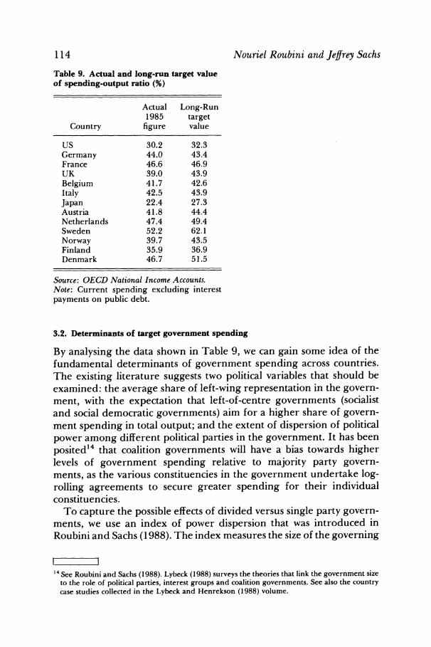
We can recover for each country an estimated target value of G/Y, the share of government spending in GNP. The estimates of the long- run target of G/Y, and the actual values of G/Y for 1985, are shown in Table 9. We can see immediately that the estimated long-run target values are quite plausible. For most countries, the actual spending levels in 1985 were very close to the estimated target levels. (This is consistent with the fact that G/Y stabilized in many countries by the mid-1980s). Britain, Denmark, Japan and Sweden showed the largest gaps between target and actual G/ Y values.


Table 9. Actual and long-run target value of spending-output ratio (%)

Actual Long-Run 1985 target

Country figure value

US 30.2 32.3 Germany 44.0 43.4 France 46.6 46.9 UK 39.0 43.9 Belgium 41.7 42.6 Italy 42.5 43.9 Japan 22.4 27.3 Austria 41.8 44.4 Netherlands 47.4 49.4 Sweden 52.2 62.1 Norway 39.7 43.5 Finland 35.9 36.9 Denmark 46.7 51.5

Source: OECD National Income Accounts. Note: Current spending excluding interest payments on public debt.

3.2. Determinants of target government spending

By analysing the data shown in Table 9, we can gain some idea of the fundamental determinants of government spending across countries. The existing literature suggests two political variables that should be examined: the average share of left-wing representation in the government, with the expectation that left-of-centre governments (socialist and social democratic governments) aim for a higher share of government spending in total output; and the extent of dispersion of political power among different political parties in the government. It has been

posited'4 that coalition governments will have a bias towards higher levels of government spending relative to majority party governments, as the various constituencies in the government undertake log- rolling agreements to secure greater spending for their individual constituencies.

To capture the possible effects of divided versus single party governments, we use an index of power dispersion that was introduced in Roubini and Sachs (1988). The index measures the size of the governing

14 See Roubini and Sachs (1988). Lybeck (1988) surveys the theories that link the government size to the role of political parties, interest groups and coalition governments. See also the country case studies collected in the Lybeck and Henrekson (1988) volume.

114

coalition, ranging from 0 (smallest coalition) to 3 (largest coalition):

Index 0 one-party majority parliamentary government; or presidential government, with the same party in the majority in the executive and legislative branches

1 coalition parliamentary government with two-to-three coalition partners; or presidential government, with different parties in control of the executive and legislative branches

2 coalition parliamentary government with four or more coalition partners

3 minority government

Values of the index for each country are given in Table 10. We also suggest here a third kind of determinant of government

spending, based on the idea that the different nations aim for different levels of 'real income insurance' for key groups in the society. Since the bulk of spending increases in the past 25 years has come in the form of increased transfer payments,. rather than the more traditional provision of final goods and services, we surmise that the demand for such spending reflects a political demand by key groups for government protection from the erosion of their real incomes in the presence of exogenous shocks. We suggest that government spending programmes are the fiscal counterpart to wage indexation schemes in the private labour market. We hypothesize that economies with widespread wage indexation arrangements are also those economies with large-scale income maintenance programmes operating through the budget.

To make this idea concrete, our idea is to use the available evidence on wage indexation across countries as a proxy for the political demands for income transfer programmes of the government. Thus, we select a variable from an earlier study of labour market institutions, an index measuring the extent of wage indexation in the economy, and use it as a proxy for the extent to which the economy is organized to protect the real incomes of the recipients of public sector transfers.15

Implicit in this approach is our belief that a widespread use of wage indexation is symptomatic of a particular style of social adjustment to external shocks, a style in which competing interest groups insist on

l l 15 The use of a preexisting measure of wage indexation for our proxy of political demands for

real income insurance has two advantages. First, it constrains the analyst from 'cooking up' a new synthetic measure that is biased towards proving a particular hypothesis. Second, it obviates the need for the very difficult task of directly measuring the extent to which the budgets of the various countries provide for guaranteed real levels of entitlements.

Fiscal policy 115


Table 10. Description of POL variable. (POL: index of the political cohesion of the national government)

US France Germany Japan UK Austria Belgium

1960 1961 1962 1963 1964 1965 1966 1967 1968 1969 1970 1971 1972 1973 1974 1975 1976 1977 1978 1979 1980 1981 1982 1983 1984 1985

0 0 0 0 0 0 0 0 0 1 1 1 1 1 1 1 1 0 0 0 0 1 1 1 1 1

1 1 1 1 1 1 1 1 1 1 1 1 1 1 1 1 1 1 1 1 1 1 1 I 1 1

1 1 1 1 1 1 1 1 1 1 1 1 1 1 1 1 1 1 1 1 1 1 1 1 1 I

0 0 0 0 0 0 0 0 0 0 0 0 0 0 0 0 0 0 0 0 0 0 0 0 0 0

0 0 0 0 0 0 0 0 0 0 0 0 0 0 0 0 0 0 0 0 0 0 0 0 0 0

1 1 1

1 1

0 0 0 0 0 0 0 0 0 0 0 0 0 0 0 0

1 1 1

O

1 1 1 1 1 1 1 1 1 1 1 1 1 2 2 2 2 2 2 2 2 2 2 2 2 2

Source: Data on national governments in Political Parties of Europe ed. by V. McHale and S. Skowronski, Greenwood Press, 1983; The Europa Yearbook, 1987.

formal claims to a given real income. We know that extensive wage indexation is prevalent in countries with labour markets characterized by a large number of powerful unions, which bargain independently for their wages, and is not very prevalent in countries with weak highly decentralized unions (e.g. the US), or in countries with a corporatist bargaining structure (in which the unions negotiate at the national or regional level).16 We hypothesize that it is in the same case, of strong intermediate

16 Calmfors and Driffill (1988) have described three basic modes of labour negotiations: highly decentralized (as in the US), with weak and dispersed labour organizations negotiating with individual employers; intermediate (as in Belgium, France, or Italy), where much more powerful, but still decentralized unions negotiate with employers; and corporatist (as in Sweden), where nationwide inclusive unions negotiate with nationwide and inclusive employers confederations. It turns out that widespread wage indexation is prevalent only in the second group of countries. It seems that corporatist economies rely on striking a national 'bargain' rather than on a specific

Fiscal policy

Table 10-continued

117

Nether- Denmark Finland Italy lands Norway Sweden Ireland

1960 1961 1962 1963 1964 1965 1966 1967 1968 1969 1970 1971 1972 1973 1974 1975 1976 1977 1978 1979 1980 1981 1982 1983 1984 1985

1 1 1 1 0 0 0 0 2 2 2 0 3 3 3 3 3 3 1 3 3 3 3 3 2 2

O

2

1 1 1 1 1 1 1 1 1 1 1 1 1 1 1 1 1 1 1 1 1 1 1 1 1 1

3 3 2 3 2 2 2 2 3 1 2 2 3 2 3 3 3 3 3 3 2 2 2 2 2 2

2 2 2 2 2 2 1 2 2 2 2 2 2 2 2 2 2 2 2 2 2 2 3 2 2 2

0 0 0 0 0 2 2 2 2 2 2 0 2 0 0 0 0 0 0 0 0 3 2 2 2 2

0 0 0 0 0 0 0 0 0 0 0 0 0 0 0 0 2 2 3 2 2 3 3 1 1 1

O 0 0 0 0 0 0 0 0 0 0 0 0 0 1 1 1 1

1

0 0 0 1 1 1

1 1

Note: France and Finland are given a score of 1 for being presidential regimes where coalition governments are usually formed. The US is given a score of 1 when there is divided power (different parties in control of the executive and legislative branch).

groups not held together in a corporatist relationship, where there will be the largest political demand for government transfer programmes (holding constant other factors, such as political orientation of the government).

Thus, we estimate a cross-section equation linking the estimated target rate of government spending to three variables: the average proportion of left-of-centre parties in the parliament, taken from Cameron (1985),

wage formula as the basic for wage setting, while in the decentralized economies, the labour groups are probably too weak in general to push for real wage protection.

Countries with high indexation according to the Bruno-Sachs index used in this paper are: Australia, Belgium, Denmark, France, Italy and the Netherlands. All of these except Denmark are judged to be 'intermediate' on the Calmfors and Driffill classification of labour markets. And of the intermediate cases in Calmfors and Driffill (Germany, the Netherlands, Belgium, Australia, France, UK and Italy), all but Germany and the UK are characterized by high wage indexation.

118

Table 11. Long-run size of the government a socio-political variables


Average Long-run % of political

target leftist stability Degree of value of governments 1973-85 indexation

Country G/Y (LEFT) (POL) (WI)

Italy 43.9 21 3.4 2 Belgium 42.6 30 2.9 2 Netherlands 49.4 22 3.1 2 Denmark 51.5 69 3.5 2 Sweden 62.1 69 2.5 1 UK 43.9 62 1.0 1 Japan 27.3 0 1.0 0 Germany 43.4 61 2.0 0 US 32.3 0 1.6 1 Austria 44.4 73 1.1 0 France 46.9 3 2.0 2 Finland 36.9 45 2.0 1 Norway 43.5 61 1.9 1

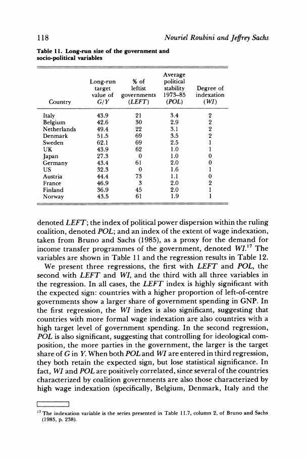
denoted LEFT; the index of political power dispersion within the ruling coalition, denoted POL; and an index of the extent of wage indexation, taken from Bruno and Sachs (1985), as a proxy for the demand for income transfer programmes of the government, denoted WI.17 The variables are shown in Table 11 and the regression results in Table 12.

We present three regressions, the first with LEFT and POL, the second with LEFT and WI, and the third with all three variables in the regression. In all cases, the LEFT index is highly significant with the expected sign: countries with a higher proportion of left-of-centre

governments show a larger share of government spending in GNP. In the first regression, the WI index is also significant, suggesting that countries with more formal wage indexation are also countries with a

high target level of government spending. In the second regression, POL is also significant, suggesting that controlling for ideological com- position, the more parties in the government, the larger is the target share of G in Y. When both POL and WI are entered in third regression, they both retain the expected sign, but lose statistical significance. In fact, WI and POL are positively correlated, since several of the countries characterized by coalition governments are also those characterized by high wage indexation (specifically, Belgium, Denmark, Italy and the

I I 17 The indexation variable is the series presented in Table 11.7, column 2, of Bruno and Sachs

(1985, p. 238).

Table 12. Effects of socio-political variables on the long-run value of the ratio of government spending to output

Alternative equations

(1) (2) (3)

Constant 0.28 0.26 0.27 (6.64) (4.90) (4.90)

LEFT 0.0023 0.0018 0.0022 (3.80) (2.89) (3.26)

WI 0.060 -0.049 (2.80) (1.30)

POL - 0.047 0.011 (2.28) (0.34)

R2 0.57 0.49 0.53

Note: t-statistics in parentheses.

Netherlands).'8 This correlation may not be coincidental: both the system of proportional representation that produces coalition governments, and the high extent of wage indexation, suggest a division of social and political power among a large number of competing, well- organized interest groups.

3.3. Cyclical factors in the growth of G/Y

We have now estimated a basic dynamic equation for G/Y, and have explored the determinants of the long-run target for G/Y.

Now, we can take the regression estimates in Table 8 and explore the implications of the econometric estimates for the effects of the output slowdown and unemployment increase on the path of G/Y in the period 1973-85. According to Table 8, the ratio G/Y rises whenever there is a slowdown of growth, or whenever there is a rise in unemployment (though the effect of rising unemployment is estimated to be smaller after 1980 than before). It follows that the 1973 and 1979 oil shocks, both of which produced a sharp slowdown in growth and an upward spurt in unemployment, led to a significant increase in the G/Y ratio in the OECD economies.

One simple way to measure the overall impact of the cyclical shocks after 1973 is to use the estimates in Table 8 to measure the cumulative effect of the growth slowdown and of the rise in unemployment on the

I I 18 This multicollinearity between POL and WI is the likely cause of the weakening of the statistical

significance of these variables when they are jointly entered in the regression.

Fiscal policy 119


spending-output ratio. We consider a counterfactual in which unemployment after 1972 remains at the 1972 level, and output growth during 1973-85 is held fixed at the rate observed during 1970-72. By 1980 the counterfactual path has a value of G/Y which is more than two percentage points below the actual 1980 G/ Y ratio in five countries: Belgium, Denmark, France, the Netherlands and the UK. In this sense we can say that in these countries the impact of slower growth and higher unemployment after 1973 had added at least two percentage points to the spending-output ratio by 1980. Continuing the counterfactual through to 1985 we find that the disparity between 1985 counterfactual and actual values of the spending ratio was less than two percentage points in all countries except the Netherlands and Belgium.19

Thus, while the growth slowdown and increase in unemployment contributed significantly to the rise in G/Y, especially in the 1970s, by 1985 much of these cyclical effects had disappeared. Clearly, it is the underlying trend factors that account for the great bulk of the cumulative increase in the spending-output ratio during 1973-85.

3.4. The dynamics of taxes and debt

We now estimate a dynamic tax equation that is similar in spirit to the equation for government spending. The purpose of the equation is to show econometrically that following a slowdown in growth or a rise in unemployment, the tax ratio T/Y does not rise rapidly enough to keep the deficit from widening.20

We suppose that the annual percentage change in the tax-output ratio follows a partial adjustment mechanism, responding with a lag to the level of the budget deficit, but also reflecting unanticipated changes in output growth and changes in the unemployment rate. We anticipate that the response to unanticipated output will be much smaller than in the corresponding equation for the spending-output ratio shown in Table 8: with tax rates largely predetermined, tax revenues depend primarily on actual income whereas spending plans reflect expected income. Similarly, we expect the rise in unemployment to have a smaller

I 1 19 The complete results are as follows. Relative to the counterfactual, the additional percentage

points on the actual G/Y which can be attributed to the shocks are: Austria (1.1, 1.4), Belgium (2.8, 3.6), Denmark (3.2, 0.8), Finland (-0.1, 1.5), France (2.9, 3.3), Germany (1.2, 1.4), Italy (-0.2, 1.0), Japan (0.5, 0.4), Netherlands (2.6, 2.9), Norway (0.1, -0.4), Sweden (-0.3, -0.7), UK (2.1, 0.4), US (1.0, -0.8) where the two numbers in parentheses refer respectively to 1980 and 1985.

20Nor should it, under Barro's theory of optimal tax smoothing, if (and this is a big if) the slowdown in growth or the rise in unemployment, is temporary. After the shocks of 1973 and 1979, however, the growth slowdown and the rise in unemployment were not quickly reversed, contrary to many expectations at the time (especially after 1973).

120

Table 13. Determinants of percentage annual growth in tax revenue to output ratio


Unanticipated output slowdown 0.44 5.1 Increase in unemployment -0.40 1.9 Changes in debt-output ratio 0.12 2.2

Note: R2 = 0.13, standard error 0.025.

effect on taxes than on spending. Indeed, if discretionary tax changes are set with Keynesian stabilization in mind, increases in unemployment will reduce tax revenue.

Table 13 shows the results, again for 1972-85 and with 13 countries. An unanticipated output slowdown increases the tax-output ratio (by reducing output) but by less than it increases the spending-output ratio in Table 8. And Table 13 suggests governments cut tax rates when unemployment rises. Thus, adverse shocks lead to sharp rises in the budget deficit and the debt-output ratio. Table 13 confirms that over the longer run a higher debt-output ratio gradually prompts tax increases to restore the fiscal position.

We also tested for a differential response to unemployment in the subperiods 1972-79 and 1980-85. In contrast to our results on spending in Table 8, we could find no statistically significant change in behaviour across the two subperiods.

Thus far, we have described the dynamics of spending (net of interest payments) and of tax revenues. Together these play the major part in accounting for the evolution of the deficit and the debt-output ratio. To complete our account, we now study the role of interest payments. The outstanding debt imposes a burden on the public finances whenever the real interest rate r exceeds the rate of real output growth n. In such circumstances the burden is higher the larger is (r-n) and the larger is the inherited debt-output ratio. We thus seek to relate changes in the debt-output ratio to the lagged debt-output ratio, to unexpected output changes, to changes in unemployment, and to a debt burden variable which is the product of (r- n) and the lagged debt-output ratio. As before we experimented with a shift term on the effect of unemployment after 1979 but we could not find any significant difference in its effect on the debt-output ratio in the two different subperiods.

In an earlier study (Roubini and Sachs, 1988) we suggested that we should also take account of the variable POL measuring the extent of dispersion of political power amongst parties of the government, since multi-party coalition governments will find it difficult to reduce deficits

Fiscal policy 121


Table 14. Determinants of annual percentage changes in the ratio of net debt to output, 1972-85

Effect of 1% change in Coefficient t-statistic

Debt-output ratio in previous year 0.79 15.5 Unanticipated output growth -0.48 6.7 Increase in unemployment 0.11 0.6 Debt burden 0.78 3.0 POL 0.0033 2.0

Note: R2 = 0.64, standard error= 0.021.

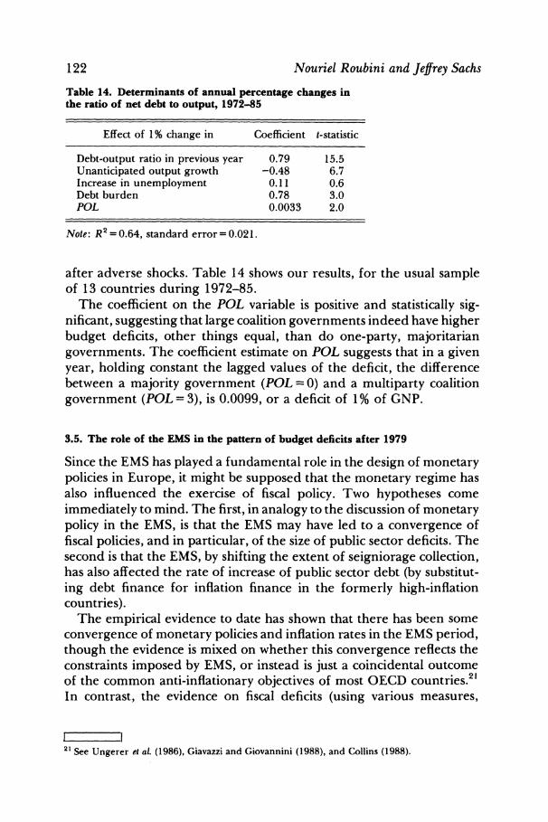
after adverse shocks. Table 14 shows our results, for the usual sample of 13 countries during 1972-85.

The coefficient on the POL variable is positive and statistically significant, suggesting that large coalition governments indeed have higher budget deficits, other things equal, than do one-party, majoritarian governments. The coefficient estimate on POL suggests that in a given year, holding constant the lagged values of the deficit, the difference between a majority government (POL = 0) and a multiparty coalition government (POL =3), is 0.0099, or a deficit of 1% of GNP.

3.5. The role of the EMS in the pattern of budget deficits after 1979

Since the EMS has played a fundamental role in the design of monetary policies in Europe, it might be supposed that the monetary regime has also influenced the exercise of fiscal policy. Two hypotheses come immediately to mind. The first, in analogy to the discussion of monetary policy in the EMS, is that the EMS may have led to a convergence of fiscal policies, and in particular, of the size of public sector deficits. The second is that the EMS, by shifting the extent of seigniorage collection, has also affected the rate of increase of public sector debt (by substitut- ing debt finance for inflation finance in the formerly high-inflation countries).

The empirical evidence to date has shown that there has been some convergence of monetary policies and inflation rates in the EMS period, though the evidence is mixed on whether this convergence reflects the constraints imposed by EMS, or instead is just a coincidental outcome of the common anti-inflationary objectives of most OECD countries.21 In contrast, the evidence on fiscal deficits (using various measures,

21 See Ungerer e a (1986), Giavazzi and Giovannini (1988), and Collins (1988). 21 See Ungerer et al. (1986), Giavazzi and Giovannini (1988), and Collins (1988).

122

including the primary deficit, total PSBR, and changes in the debt-to- GDP ratios) shows no evidence of fiscal convergence. If anything, one observes some degree of fiscal divergence, as most measures of dispersion of deficits rose among the EMS group of countries after 1979. Basically, Italy, Belgium, the Netherlands and Ireland had larger deficits after 1979 than before, while the deficits in Germany and Denmark declined markedly.

This absence of fiscal convergence is not really surprising, since the constraints imposed on fiscal policy by the requirement of pegging the exchange rate are very long-run constraints. In the short run, a given nominal exchange-rate target can be consistent with a very wide range of fiscal policies, assuming that the government has access to domestic and international borrowing. This point is especially true in cases where capital controls have been operative. (See Roubini, 1988, on these points).

On the question of the links of the EMS to seigniorage collection, and of seigniorage collection to the rise of the debt-to-GNP ratio, the evidence is mixed. The hypothesis is that the EMS induced a slowdown in inflation in the member countries outside of Germany, as they undertook the commitment to peg to the Deutsche Mark. As a result, they experienced a reduction in seigniorage collections. If the lost seigniorage was not fully compensated for by higher taxes or lower spending, we should observe a faster rise in the debt-GNP ratio. We find that, on average, a reduction of seigniorage collections after 1979 is indeed associated with a faster growth of the debt-to-GNP ratio. The tradeoff even appears to be approximately one-for-one: lower seigniorage after 1979 translated fully into higher debt accumulation.

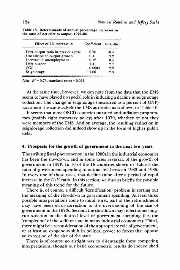
To perform the test in a simple manner, we estimate the cross-section, time-series equation for the change in debt (Table 14) and add the annual seigniorage as an additional variable.22 The results are shown in Table 15. The coefficient on the seigniorage variable is negative and statistically significant. The other variables all maintain their signs and statistical significance from the earlier estimation. The equation suggests that each 1% of GNP reduction in seigniorage was associated with a rise in the debt-GNP ratio of around 1%. In other words, over this period, it appears that indeed, seigniorage and public debt accumulation were close substitutes. The reduction in seigniorage did not really solve the fiscal problems of the high-inflation countries: it just pushed the problems into the future in the form of a higher stock of public debt.

I 1 22

Seigniorage is measured as a percent of GNP as (M - M_,)/ Y,, where M, is end-of-period base money, and Y, is nominal GNP. The data are taken from International Financial Statistics, IMF, and M is taken from line 14 ('reserve money') for each country.

Fiscal policy 123


Table 15. Determinants of annual percentage increases in the ratio of net debt to output, 1979-85


Debt-output ratio in previous year 0.76 10.5 Unanticipated output growth -0.41 3.2 Increase in unemployment 0.12 0.5 Debt burden 1.41 2.7 POL 0.0083 2.9 Seigniorage -1.06 2.3

Note: R2= 0.73, standard error = 0.021.

At the same time, however, we can note from the data that the EMS seems to have played no special role in inducing a decline in seigniorage collection. The change in seigniorage (measured as a percent of GNP) was about the same outside the EMS as inside, as is shown in Table 16.

It seems that most OECD countries pursued anti-inflation programmes (mainly tight monetary policy) after 1979, whether or not they were members of the EMS. And on average, the resulting reduction in seigniorage collection did indeed show up in the form of higher public debt.

4. Prospects for the growth of government in the next few years

The striking fiscal phenomenon in the 1980s in the industrial economies has been the slowdown, and in some cases reversal, of the growth of government in GNP. In 10 of the 15 countries shown in Table 3 the ratio of government spending to output fell between 1983 and 1985. In every one of those cases, that decline came after a period of rapid increase in the G/Y ratio. In this section, we discuss briefly the possible meaning of this trend for the future.

There is, of course, a difficult 'identification' problem in sorting out the meaning of the slowdown in government spending. At least three possible interpretations come to mind. First, part of the retrenchment may have been error-correction to the overshooting of the size of government in the 1970s. Second, the slowdown may reflect some long- run satiation in the desired level of government spending (i.e. the 'completion' of the welfare state in many industrial economies). Third, there might be a reconsideration of the appropriate role of government, or at least an exogenous shift in political power to forces that oppose an extension of the size of the state.

There is of course no airtight way to disentangle these competing interpretations, though our basic econometric results do indeed shed

124

Fiscal policy Table 16. Seigniorage as percentage of GDP (annual averages)

1975-79 1980-85 Increase

125

EMS: Germany 0.78 0.18 -0.60 France 0.03 0.70 0.67 Italy 3.55 1.96 -1.59 Belgium 0.74 0.10 -0.64 Netherlands 0.57 0.43 -0.14 Denmark* 0.39 0.95 0.56 Ireland 2.15 0.83 -1.32

Average 1.17 0.73 -0.43 EEC, non-EMS

UK 0.70 0.02 -0.68 Spain 2.33 3.17 0.84 Greece 2.87 3.85 0.98 Portugal 4.17 3.45 -0.72

Average 2.51 2.62 0.10 non-EEC

US 0.47 0.34 -0.13 Japan 0.77 0.49 -0.28 Canada 0.62 0.20 -0.42 Austria 0.94 0.49 -0.45 Finland 0.49 0.75 0.26 Norway 1.02 0.43 -0.59 Sweden 0.96 0.20 -0.76 Australia 0.62 0.53 -0.09 Switzerland 1.04 0.19 -0.85

Average 0.77 0.39 -0.38

Sources: IMF-IFS Data. Note: The Danish figure is biased by a large outlier for 1985.

some light on these questions. In principle, our framework allows for a separation of the first and second considerations, i.e., the cyclical effects on G/Y versus the effects of satiation in the public demand for G/Y. We saw earlier that according to our estimates, most countries were still under, but close to, their long-run target levels of G/Y. Only Germany is measured to be above the long-run target; the US, France, Italy, Austria, the Netherlands and Norway are estimated to be close to, but below, equilibrium; and Japan, Denmark and Sweden are still estimated to be closing in on significantly higher levels of G/Y.

The equations also suggest that an increase in output growth, or reduction in unemployment, is likely to have a significant cyclical effect on the share of spending in GNP (and of course on the budget deficit). There are many signs that after 15 years of relative stagnation, the European economies are beginning to grow again at respectable rates (of around 4% per year), enough finally to bring the high unemployment


rates down. Both the rise in GNP growth and the fall in unemployment rates auger for a further drop in the G/Y ratio in the next couple of years.

Of course, all of this evidence is much too crude to evaluate the third possibility: that there has been a significant conceptual change in think- ing about the role of government in the economy, that will lead to a significant retrenchment of G/Y. This may in fact be occurring, but our crude statistical techniques could not tell us so with any confidence. For that, we would have to delve much more deeply, and on a country- by-country basis, into political and social trends, perhaps using survey data rather than macroeconomic time-series data.

5. Conclusions

In this paper, we have tried to interpret several important trends in the size of governments and government deficits in the OECD economies. We noted three phenomena of central importance: the rapid increase in G/Y in the period after 1965, and particularly after 1973; the sharp rise in budget deficits and in debt-GNP ratios after 1973; and the early signs of a slowdown or reversal in the rise of G/Y in the 1980s. We have tried to offer some economic and political interpretations of each of these findings.

With respect to the first, we noted that the rise in G/ Y was importantly associated with the slowdown in growth after 1973, as well as with the gradual adjustment of G/Y to a long-run target value. That long-run value itself was shown to depend on the political and institutional characteristics of the various economies.

As for budget deficits, we showed that much could be explained by normal cyclical factors (the slowdown in growth and the rise in unemployment after 1973), but that in addition, the size of the budget deficits was related to political as well as economic characteristics of the countries. Budget reduction requires political consensus, at least among the members of the government. We noted that such consensus was harder to achieve in multi-party coalition governments (as in Belgium and Italy), and that the failure to reach a consensus on budget cutting could help to explain why such countries have experienced such an enormous rise in the debt-GNP ratio.

We also digressed briefly to consider whether the EMS had played any apparent role in budgetary policy of the member governments. We found little evidence of policy convergence among the EMS members, and also little evidence that the EMS had played a special role in reducing seigniorage financing. We did note, however, that governments which cut their seigniorage collections after 1979 seemed to finance that

126

reduction through a faster accumulation of public debt. In other words, public borrowing was substituted for the inflation tax after 1979.

At the end of the paper, we explored briefly the possible explanations for the slowdown in the growth of G/ Y in the most recent years, and the implications for the future. Our conclusions were necessarily cautious. We noted that the estimated equations suggested that most, though not all, of the industrial countries were now very close to their long-run target levels of G/Y. We also pointed out that the incipient 'mini-boom' in many countries in Europe suggested a further drop in G/Y in future years. But at the same time, we necessarily left open the possibility that recent trends reflect not merely a satiation of G/Y, but also a reconsideration of the appropriate role of government, that might lead to a retrenchment of G/ Y in the future. The macroeconomic data do not yet suggest such a shift, but the time-series macroeconomic evidence is much too weak to make any conclusive statements in this regard.

Discussion Seppo Honkapohja Yrjo Jahnsson Foundation, Helsinki

The authors provide a sweeping and thought-provoking analysis of government scale and government finance in OECD countries. The first two sections set the scene in some detail though, given the significance of the oil crises, I would have liked more annual data, country by country, on how government expenditure was affected at these times. It would also be useful to have a more detailed perspective on the (very different) reactions to the second oil shock.

The interesting cross-country analysis is in Section 3. Sachs and Roubini test whether political factors can explain cross-country differences in responses. I find plausible their conclusion that coalition governments found it harder quickly to make the required response to adverse shocks, and instead allowed debt to accumulate. The central message is that transitional difficulties can affect rather long-run trends.

For government expenditure, the results are less satisfactory. The two episodes 1973-79 and 1979-85 are very different. The effect of the growth slowdown variable is much more important in the earlier period, yet the influence of wage indexation is much more significant in the later period. Overall the authors find it harder to explain the latter period. Can we explain these findings? My tentative view is that perceptions of the permanence of the shock, and hence the required adjustment, were more accurate in the second episode. Differences must refer to expectations as well as merely political variables.

Fiscal policy 127


Table 1A. Error correction and the change in net debt

Error Change in correction Trend effect

net debt effect 1983-85 earlier 1983-85

US 3 0 up up Germany 28 0.2 up down France 9 0.1 up down UK -19 0 up up Italy 40 0.4 up up Canada 31 0.1 up up Belgium 61 0.2 up down Finland 7 0.1 up up Austria 30 0 up down Netherlands 22 -0.1 up down Sweden 44 -0.1 up down Norway -23 0.1 up down

Sachs and Roubini emphasize 'error correction' or gradual adjustment towards the desired long-run ratio of spending to output. An alternative interpretation is suggested by Table 1A.

First, countries which still had an upward trend in spending/output tend to be those with a small increase in net debt. Second, those with a large increase in net debt tended to reverse the upward trend in spending relative to output. Third, there is no strong correlation of the error correction effect with the change in net debt.

Perhaps past deficits and changes in debt exert some influence on government spending via the trend. If so, countries with rather large debt increases during 1972-85 will have to continue to cut back spending in the future, whilst those whose debt position is now under control may be able to avoid such pressures. Elsewhere in this volume, Rudiger Dornbusch considers how Ireland will be likely to respond to the challenge of a soaring debt burden.

Daniel Cohen CEPREMAP, Paris

Is Wagner's law a reflection of: (1) an increasing demand for public spending (which is, incidentally, Wagner's own view) or: (2) an artefact of democracy which always finds it easier to raise public spending than to resist vested interests? Partisans of the first view will point to the fact that spending on health education and the like is no lower in countries where these are privately managed than in countries where they are publicly run. Partisans of the second view will point to the fact that public spending has not fallen for the past two centuries as a proportion

128

of GNP, even when it might have been expected to do so (such as at the end of a war).

The argument in Roubini and Sachs' paper is that public spending is more likely to rise in badly-functioning economies. Regressions are shown to prove that, for example, countries in which wages are relatively rigid are also those where public spending is the highest. From this (interesting) piece of evidence, the authors argue that: 'the same factors which led to excessive real wage growth and high unemployment also led to excessive public sector growth. Thus, we distinguish between economies in which organized interests are able to protect the growth of real income (in this case, transfers and public goods received from the public sector) and those economies in which they are not.'

In other words, Wagner's law is interpreted through its 'anti-democratic' version: it is the weakness of politicians which explains the large deficits observed in the 1980s. In order to make that point, multi-party coalition governments are shown to have presided over the largest changes in the debt-to-GDP ratio. The interpretation is that multi-party coalitions are more dependent upon the pressure of interest groups than are majority governments.

How does this view differ from the 'public choice' approach to the problem? One difference - suggested by the authors themselves - is that prior to 1973 there are no major discrepancies in the public spending-to- GDP ratio of the major industrialized countries (as Buchanan and others would suggest) while the response to the 1973 crisis reveals striking discrepancies.

This is certainly an interesting fact, but what is the explanation? Why did interest groups pressure weak governments only after the crisis? If a weak democracy is more likely to accept the pressure of lobbies, why did the weak democracies (multi-party coalitions, for example) not exhibit larger ratios of debt to GDP or of public spending to GDP before the 1973 crisis?

I would think that there are (at least) two ways of answering these questions. One is to accept the first interpretation of Wagner's law and to interpret post-1973 behaviour as an optimal response of the governments to the crisis that they faced. Granted that ill-functioning labour markets are more likely to generate large unemployment, it is not surprising that governments would then step in to correct the disequili- bria in the economy through subsidies, unemployment programmes and so on.

Another view (consistent with the second interpretation of Wagner's law) is that government intervention tried to alleviate a crisis which turned out to last longer than was at first anticipated. The flaw of multi-party coalitions is then not that they cannot resist the pressure of

Fiscal policy 129


lobbies but that they are penalized less (in terms of losing elections) when they manage the economy badly. This is in fact the view adopted by Karl Popper who argued that two-party democracies are stronger than multi-party democracies because a bad government in a two-party democracy loses elections to the opposition. In multi-party coalitions, it is always more difficult for the electorate to turn out the government. Errors of judgement in economic policy can then last longer.

If this is what explains why weak democracies experienced larger deficits after the crisis (and not beforehand) the paper by Roubini and Sachs is bound to become anachronistic: the crisis of fiscal policy must be ending, now that all governments (or almost all) acknowledge it.

General discussion

Colin Mayer started the discussion by pointing out that extensive privatization programmes could distort the data on government debt. When privatizations are realized there is an improvement in the government debt position, which is matched by a deterioration in the net equity position, so that net wealth is unaffected. He also regretted that the data on government budget balances had not been adjusted for cyclical fluctuations and inflation. Still with respect to data problems, Manfred Neumann warned that indices, like the index of political cohesion, were qualitative. As a result, in a regression, only the sign, and not the magnitude, of its coefficient is meaningful.

Jean-Pierre Danthine recommended caution about the observation that an increase in the ratio of government expenditures to income could be positively related to wage indexation. He found plausible the authors' interpretation that wage indexation reflects the degree of protection of real government transfers. Yet he suggested a more mechanical interpretation of this positive relationship: the extent of

wage indexation could presumably be related to the level of unemployment, and hence the level of unemployment benefits, thereby automati- cally increasing the ratio of government expenditure to income. Jeffrey Sachs indicated in response that the slowdown in income and the rise in unemployment had been controlled for, to the extent possible. He acknowledged that a direct estimation of the changes in income transfer would provide useful additional evidence. Mayer was equally cautious about the explanations behind the change in the ratio of government expenditure to income, but for another reason; he thought that governments in the mid-1970s might have perceived that the effect of the energy crisis on their permanent income was likely to be rather small. Presumably, the British and Norwegian governments would have been

130

right to think so, in anticipation of North Sea oil revenues. As a result, the increase in government expenditures relative to income might simply reflect a deliberate absence of policy response.

Victor Norman expressed doubts about the use of the indexation variable as a proxy for the degree of protection of real transfers. He argued that this indexation variable was really trying to capture the extent to which a country was able to handle distributional matters. Along those lines, he found it disturbing that the Nordic countries did not seem to fit the general pattern. With a high degree of wage indexation and centralized bargaining, these countries were expected to do relatively well in terms of adjustment in government expenditures. Yet this is not the case. Norman's interpretation was that favourable labour market arrangements are not indicative, in Nordic countries, of an ability to handle distributional matters. Quite to the contrary, it seems that Nordic countries are very fragmented in every other respect than the labour market. Along similar lines, Sushil Wadhwani recalled that corporatist countries also tend to have a comprehensive social security system and that improvements in welfare benefits are sometimes used as a bargaining tool in wage negotiations.

With respect to the index of political cohesion, Alberto Alesina suggested another justification for assessing political cohesion partly in terms of the number of coalition members. According to Alesina, a high number of coalition members should lead to more polarization and a higher degree of ideological diversity, which should result in more difficult negotiations. Rainer Masera pointed out a counter- example to the validity of the index, according to which minority governments have the worst score: the first government which managed to change expenditure laws in Italy was actually a minority government. Norman also argued that majority governments should not necessarily have the highest score, given that a ruling party is in many ways a coalition in itself. It was also suggested by several panel members that, rather than define political cohesion in terms of observed political outcomes, one should derive it from the characteristics of the electoral system. In response, Sachs acknowledged that this would be desirable but was confident that the cross-country difference would not be affected. Sachs also addressed Daniel Cohen's presumption that countries lacking political cohesion should have experienced higher growth of government expenditure prior to the consolidation period. He argued that coalition governments do not malfunction to the same extent in good and bad times; what makes a coalition government vulnerable is the veto right effectively granted to each of its members. The exercise of this right is often avoided in good times.

Fiscal policy 131


References

Barro, R. (1979). 'On the Determination of Public Debt', Journal of Political Economy. --(1987). 'Government Spending, Interest Rates, Prices, and Budget Deficits in the United

Kingdom, 1701-1918', Journal of Monetary Economics. Bruno, M. and J. Sachs (1985). Economics of Worldwide Stagflation, Harvard University Press. Calmfors, L. and J. Driffill (1988). 'Bargaining Structure, Corporatism and Macroeconomic

Performance', Economic Policy. Cameron, D. R. (1978). 'The Expansion of the Public Economy: A Comparative Analysis', American

Political Science Review. --(1985). 'Does Government Cause Inflation? Taxes, Spending and Deficits', in L. Lindberg

and C. Maier (eds.) The Politics of Inflation and Economic Stagnation, The Brookings Institution, Washington, D.C.

Cohen, D. (1988). 'What Caused the Rise of Conservatism: A French View', Economic Policy. Collins, S. (1988). 'Inflation and the EMS', mimeo, Harvard University. Emerson, M. (1986). 'What Model for Europe'?, mimeo, Harvard University. Giavazzi, F. and A. Giovannini (1988). Limiting Exchange Rate Flexibility: The European Monetary

System, forthcoming, M.I.T. Press. Larkey, P. D., C. Stolp and M. Winer (1981). 'Theorizing about the Growth of Government: A

Research Assessment', Journal of Public Policy. Lybeck, J. A. (1986). The Growth of Government in Developed Economies, Aldershot: Gower Press. --(1988). 'Comparing Government Growth Rates: The Non-Institutional vs. the Institutional

Approach' in Lybeck, J. A. and H. Henrekson (eds.) Explaining the Growth of Government, North-Holland.

Lybeck, J. A. and H. Henrekson (1988). (eds.) Explaining the Growth of Government, North-Holland. Mueller, D. C. (1987). 'The Growth of Government: A Public Choice Perspective', IMFStaff Papers. OECD (1985). 'The Role of the Public Sector', OECD Economic Studies, No. 4 Spring. Ram, R. (1987). 'Wagner Hypothesis in Time-Series and Cross-Section Data Perspectives: Evidence

from 'Real' Data for 115 Countries', Review of Economics and Statistics. Roubini, N. (1988). 'International Transmission of Macro Policies under Alternative Exchange

Rate Regimes: A Four Country Model', mimeo, Harvard University. Roubini, N. and J. Sachs (1988). 'Political Economic Determinants of Budget Deficits in the

Industrial Economies', NBER Working Paper No. 2682, forthcoming in European Economic Review, 1989.

Schmidt, M. G. (1982). Wohlfahrtsstaatliche Politik unter burgelichen und Sozialdemokratischen Regierungen; ein Internationaler Vergleich, Frankfurt: Campus Verlag.

- (1983). 'The Growth of the Tax State: The Industrial Democracies, 1950-1978', in C. L. Taylor (ed.) Why Governments Grow, Beverly Hills: Sage Publications.

Tarschys, D. (1975). 'The Growth of Public Expenditures-Nine Modes of Explanation', Scandinavian Political Studies.

Ungerer, H., O. Evans, T. Mayer and P. Young (1986). 'The European Monetary System: Recent Developments', Occasional Paper No. 48, December.

Wagner (1877, 1890). Finanzwissenschaft, Vol I and II, Leipzig: C. F. Winter.

Government Spending and Budget Deficits in the …homepage.ntu.edu.tw/~kslin/macro2009/Roubini and...

Documents

Transcript of Government Spending and Budget Deficits in the …homepage.ntu.edu.tw/~kslin/macro2009/Roubini and...