Government Debt and Risk Premia

Yang Liu∗

November 23, 2016

Abstract

I document that government debt is related to risk premia in various asset markets: (i) the

debt-to-GDP ratio positively predicts excess stock returns with out-of-sample R2 up to 30%

at a five-year horizon, outperforming many popular predictors; (ii) the debt-to-GDP ratio is

positively correlated with credit risk premia in both corporate bond excess returns and yield

spreads; (iii) higher debt-to-GDP ratio is associated with lower real risk-free rates, (iv) higher

debt-to-GDP ratio corresponds to lower average expected returns on government debt; (v) debt-

to-GDP ratio positively comoves with fiscal policy uncertainty. I rationalize these empirical

findings in a general equilibrium model featuring recursive preferences, endogenous growth,

distortionary taxation, and time-varying fiscal uncertainty. In the model, the tax risk premium

is sizable and its time variation is driven by fiscal uncertainty. Furthermore, the model gener-

ates an endogenous relationship between the debt-to-GDP ratio and fiscal uncertainty. Fiscal

uncertainty increases debt valuation through lower government discount rate. This mechanism

is reinforced as higher debt conversely raises uncertainty because of future fiscal consolida-

tions. (JEL E62, G12, G17, H63)

∗Yang Liu (liuyang5@sas.upenn.edu) is at the Department of Economics, University of Pennsylvania, 3718 Lo-cust Walk, Philadelphia, PA 19104. I am immensely grateful to my advisors Amir Yaron, Enrique Mendoza, FrankSchorfheide, and Ivan Shaliastovich for their invaluable guidance and advice. I also thank Ravi Bansal, Ric Colacito,Hal Cole, Max Croce, João Gomes, Urban Jermann, Dirk Krueger, Nick Roussanov, Tom Sargent, Lukas Schmid,and seminar participants at Penn, Wharton, Philly Fed, and EconCon for helpful discussions. I thank George Hall forgovernment debt data. All errors are my own.

1

1. Introduction

The government debt is of great importance to the economy, policymaking, and financial markets.This paper documents a set of new facts about the effects of government debt on asset prices inthe United States. High debt-to-GDP ratios are related to high equity risk premia, high creditrisk premia, low risk-free rates, low expected returns on government debt, and high fiscal policyuncertainty. I rationalize these facts in a general equilibrium model featuring a fiscal uncertaintychannel that links government debt and asset prices.

The importance of government debt is manifested in equity, credit and treasury markets. First,high debt-to-GDP ratio corresponds to high equity premium. The debt-to-GDP ratio positivelypredicts excess stock returns at horizons from one quarter to five years. The ratio contains usefulinformation beyond a large number of existing predictors, thus improving the predictive power.In a univariate predictive regression using debt-to-GDP ratio, the out-of-sample R2 is 10% at anannual horizon and reaches 30% at a five-year horizon. In comparison, the out-of-sample R2 ofmany popular predictors are marginally positive. A strategy that times the market using debt-to-GDP ratio can generate an excess return of 14.71% per annum with a Sharpe ratio of 0.66, while abuy and hold strategy of the market portfolio yields a Sharpe ratio of 0.3.

In credit markets, I observe a similar pattern that high debt-to-GDP ratios are related to highcredit risk premia. One measure of credit risk premia is the expected excess return on corporatebonds. The debt-to-GDP ratio positively predicts excess returns on investment-grade and high-yield corporate bonds. The magnitude is close to the stock return predictability. Another measureof credit risk premium is a yield spread. I document that government debt raises the credit premiumcomponent of yield spreads.

The first two findings show that high debt-to-GDP ratio implies high cost of capital for firms.Regarding the cost of capital for government, however, high debt-to-GDP ratios are associated withlow real risk-free rates and low expected returns on government debt. Both 1-month and 3-monthreal risk-free rates are negatively related to the debt-to-GDP ratio, controlling for expected growthand inflation. Furthermore, I examine the discount rate of the government. Since the governmentdoes not only issue short-term debt, the government discount rate or effective borrowing cost is theaverage return across terms to maturity on all the Treasury securities. In the default-free case, thegovernment budget constraint implies that a high debt-to-GDP ratio can stem from three channels:(i) high expected future primary surplus to pay off the debt, (ii) high expected future growth tostabilize the ratio, and (iii) low expected future returns on government debt. The previous studiesmainly focus on the first two channels. Here I document that the third discount rate channel isempirically important:1 the debt-to-GDP ratio negatively predicts returns on government debt. I

1This discount rate channel is addressed differently in several papers. Hall and Sargent (2011) show variations inrealized returns affect the evolution of the debt-GDP ratio. Berndt et al. (2012) find that part of a fiscal spending shock

2

use a present value decomposition in a vector autoregression to quantify the relative contributionof these three components. The variation of expected returns accounts for 25% of the variation ofthe debt-to-GDP ratio.

Why does government debt have such significant effects on asset prices? Major existing chan-nels of government debt such as liquidity, safety, and crowding out are silent or inconsistent withthese facts. I propose a new channel—fiscal uncertainty—that can rationalize the empirical find-ings jointly. I propose a broad-based measure of fiscal policy uncertainty by utilizing 169 macrovariables and estimating a dynamic factor model with stochastic volatility. In the data-rich envi-ronment, fiscal policy consists of 37 variables regarding various types of tax, spending and transfer.Fiscal uncertainty is measured as the common component of the conditional forecast error volatilityof these fiscal policy instruments. Empirically, fiscal uncertainty fluctuates over time and positivelycomoves with the debt-to-GDP ratio with a correlation of 0.5. Therefore, government debt encodesthe risks in fiscal policy that drive the variation of risk premia. I present direct evidence that fiscaluncertainty affects asset prices in equity, credit, and treasury markets in the same directions andhas similar magnitudes as the debt-to-GDP ratio.

Within a general equilibrium model, I quantify the effects of government debt and fiscal uncer-tainty on asset prices. The key ingredients of the model include recursive preferences, endogenousgrowth through innovation, and fluctuations in the volatility of distortionary corporate income tax.Tax hikes depress innovation and economic growth so that persistent tax changes are a sourceof endogenous long-run risks. Stock prices drop with tax hikes because of the tax payment andthe lower cash flow growth. For fear of the joint decrease of growth prospects and stock prices,agents demand a large equity premium for tax risks. This risk compensation is even larger whenthe “quantity” of risk increases in times of high fiscal uncertainty. Hence, time variation in equitypremium is driven by fiscal uncertainty. In contrast, non-defaultable government bonds rally intimes of high tax, because lower expected growth induces the agents to purchase safe bonds. Thus,government bonds hedge against tax risks for investors and have negative risk premia. In time ofhigh fiscal uncertainty, the hedging motive drives down the government bond premium. Moreover,uncertainty increases the precautionary saving motive and lowers the risk-free rate.

The model generates a positive comovement between the debt-to-GDP ratio and fiscal uncer-tainty through two mechanisms. Uncertainty lowers both risk-free rate and bond risk premium andthus the expected return on government debt. The declining expected return leads to the rise ofthe bond price. Therefore, the debt-to-GDP ratio increases with uncertainty through the discountrate channel. Conversely, debt generates uncertainty in future fiscal policy. The government im-plements fiscal consolidations from time to time to reduce deficits and debt accumulation. Theconsolidation policy is uncertain and anticipated to be more active when debt is high. As a result,

is financed with decreases in the discount rate.

3

high debt-to-GDP ratio brings more uncertainty in fiscal consolidations. The two mechanismsreinforce each other. In equilibrium, the debt-to-GDP ratio reveals fiscal uncertainty and has im-plications for asset prices that are consistent with the empirical findings. Calibrated to fiscal policydata, the model quantitatively explains many features of macroeconomics dynamics and asset mar-kets such as equity premium and risk-free rate, as well as the novel facts regarding the governmentdebt.Relation to Literature. There is a long-lasting debate on the effects of government debt on inter-est rate (Elmendorf and Mankiw, 1999; Engen and Hubbard, 2005; Laubach, 2009). Few papersconsider the importance of risk premia across different interest-bearing instruments. Distinguish-ing between real risk-free rate, return on equity, corporate bonds, and government debt, I show thathigh government debt is associated with high cost of capital for firms and low cost of capital forgovernment. Krishnamurthy and Vissing-Jorgensen (2012) find that high government debt is re-lated to lower spreads between assets with different liquidity and safety attributes.2 My evidence ofthe effect of government debt on credit risk premia is complementary to their evidence of liquiditypremia. Croce et al. (2016) show that debt-to-GDP ratio predicts the spreads between innovation-sorted stock portfolios in the time series and cross section, while I focus on the aggregate assetmarkets. Greenwood and Vayanos (2014) document that the maturity structure of government debtaffects nominal bond risk premia and term spreads.

I contribute to the voluminous literature of stock return predictability by analyzing debt-to-GDP ratio as a predictor. The results have little bias from the high persistence of the debt-to-GDP ratio (Campbell and Yogo, 2006; Stambaugh, 1999). The out-of-sample predictive poweris compelling (Welch and Goyal, 2008). Debt-to-GDP ratio outperforms the popular predictorsregarding out-of-sample mean squared error.3

A long theoretical literature links government debt to macroeconomic dynamics. RicardianEquivalence states that government debt has no effect in a frictionless standard representative-agent model (Barro, 1974). However, in the presence of liquidity and safety needs, governmentdebt plays a special role and has significant effects on macroeconomic quantities and asset prices(Bansal and Coleman, 1996; Krishnamurthy and Vissing-Jorgensen, 2012; Gorton and Ordonez,2013; Drechsler et al., 2014; Greenwood et al., 2015). The impact of government debt is also largein heterogeneous agent incomplete market models (Gomes et al., 2013). These theories are ei-ther silent on the new empirical findings or have counterfactual implications that high government

2Graham et al. (2014) document a similar negative relationship between debt-to-GDP ratio and Baa-Aaa spread.They also find that government debt has large impacts on corporate financing and investment policies.

3Some of the major predictors are the dividend-price ratio (Campbell and Shiller, 1988), book-to-market ratio(Kothari and Shanken, 1997), term spread (Fama and French, 1989), short rate (Hodrick, 1992; Ang and Bekaert,2007), investment rate (Cochrane, 1991), the consumption-wealth ratio (Lettau and Ludvigson, 2001), output gap(Cooper and Priestley, 2009), and government investment rate (Belo and Yu, 2013).

4

debt is related to low equity premium and high risk-free rate. I contribute to the understanding ofgovernment debt by proposing a new fiscal policy uncertainty channel which operates through thegovernment discount rate and also affects other risk premia. Because debt-to-GDP ratio encodesthe variation of fiscal uncertainty, it explains risk premium variation, which complements the ex-isting explanations of time-varying risk aversion (Campbell and Cochrane, 1999), time-varyingconsumption volatility (Bansal and Yaron, 2004), and time-varying risk of disasters (Wachter,2013).

My analysis of fiscal uncertainty also relates to the recent literature examining the role of eco-nomic uncertainty both in the data and models (Bloom, 2009; Bansal et al., 2014; Jurado et al.,2015, among others). Pástor and Veronesi (2013) and Baker et al. (2015) study the asset pricingand macroeconomic impacts of general economic policy uncertainty. Fernández-Villaverde et al.(2015) and Born and Pfeifer (2014) show the importance of fiscal uncertainty on economic activi-ties. I propose a new broad-based measure of fiscal policy uncertainty and illustrate its importancefor asset prices.

More broadly, this article belongs to the growing literature studying asset prices in a productioneconomy (Jermann, 1998; Croce, 2014). Similar to Kung and Schmid (2015) and Kung (2015), Iendogenize the long run risks (Bansal and Yaron, 2004) in a expanding variety endogenous growthmodel (Romer, 1990).4 The long run risks are purely driven by productivity shocks in Kung andSchmid (2015), whereas part of the long run risks rise from tax policy in my model. Croce et al.(2012) demonstrate a sizable tax risk premium in a model with capital structure choice where taxrate drives the technology growth exogenously.

The remainder of the paper is organized as follows. Section 2 documents the empirical findings.Section 3 lays out the model. Section 4 presents the economic mechanism and the quantitativeimplications of the model. Section 5 concludes.

2. Empirical Evidence

In this section, I document the new facts that high government debt-to-GDP ratio is related tohigh equity risk premium, high credit risk premium, low risk-free rate, low expected return ongovernment debt, and high fiscal policy uncertainty.

2.1 Data Description

Government debt is defined as the market value of the federal government debt held by the pub-lic. The market value of government debt is constructed by summing up the market value of allthe credit market instruments across maturities (Treasury bonds, Treasury botes, Treasury bills,

4Comin and Gertler (2006) study business cycle and long-run dynamics in a unified endogenous growth model.

5

TIPS, etc). Government debt data are from Dallas Fed, Flow of Funds and, George Hall (Hall andSargent, 2011). Figure 1 demonstrates the time series plot of the debt-to-GDP ratio. The ratio dou-bled from 20% to 40% during the Great Depression and jumped to 100% around the second worldwar. It declined gradually in the peacetime expansion until the early 1970s. Congress increasedits control on the government budget process after the Congressional Budget and ImpoundmentControl Act of 1974, leading to deficits and rising debt. In the 1980s, President Reagan’s tax cutsand military buildup further increased the debt. The fiscal balance returned to a surplus in the termof President Clinton, due to tax increases, military spending decreases, and an economic boom.Finally, the Great Recession, combined with Bush tax cuts, caused expanding government expen-diture and declining revenue. In 2014, the ratio reached its post-war peak. One crucial featureis that the debt-to-GDP ratio is driven mainly by military and political issues and fiscal policy re-forms. While the debt-to-GDP ratio rises in NBER recessions, it does not tend to decline in normaltimes. In fact, the business cycle only accounts for a small proportion of its variance.

The asset prices data are obtained from CRSP, Barclay and Fred. The average return on gov-ernment debt is from George Hall. The stock return predictors are from Amit Goyal’s website. Thedata on macroeconomic and fiscal variables are from NIPA and FRED-QD database (McCrackenand Ng, 2016). The detailed explanations of the data are in the appendix.

2.2 Equity Premium

After studying the time series property of the debt-to-GDP ratio, I show that it strongly predictsfuture excess stock returns in sample and out of sample.

2.2.1 In-sample Tests

Table 1 reports the results from OLS regressions of future excess stock returns on log debt-to-GDPratio. Excess stock return is the log market return subtracting the log risk-free rate. Long-horizonexcess returns are the cumulative summation of the one-period excess returns. In the sample from1926 to 2014, higher debt-to-GDP ratio forecasts higher stock returns in the future. The forecastingpower becomes stronger at longer horizons as R2 rises from 11% at the annual horizon to 38% atthe five-year horizon. As in the previous findings, returns are more predictable at longer horizons,since the high-frequency noises are canceled out, and the slow-moving expected return is reflectedmore clearly in the data. The coefficients across all the horizons are statistically significant at 99%.In Figure 2, I plot the 5-year ahead ex-post and expected excess return. The expected excess returnis the fitted value of the predictive regressions. It is evident that higher debt-to-GDP ratio implieshigher subsequent returns. The expected excess return rises from the 1930s to the 1950s, declinesfrom the 1950s to the 1970s, and rises again from the 1970s to the 1990s and during the Great

6

Recession.Beyond the statistical significance, the economic impact of debt-to-GDP ratio on the expected

excess return is substantial. A one percentage point increase in debt-to-GDP ratio indicates a 38basis-point increase in expected excess return per annum.5 Taking the Great Recession as an ex-ample, we observe a rapid increase in the debt-to-GDP ratio from 30% to 60%. This swing impliesthat the expected return is 11.4% higher than its pre-crisis level. It is acknowledged that excessreturn predictability is equivalent to time-varying equity premium in a standard rational pricingmodel.6 Thus, the rise of debt-to-GDP ratio indicates that investors require a high premium tocompensate equity risks. The classic equity premium puzzle emphasizes the difficulty in rational-izing the 6% average equity premium given the lower risk in the consumption profile. It is nowmore puzzling in that the equity premium is largely time-varying, from 2% in 2007 to 13% in 2014.

From an asset management point of view, this large time variation of expected return is valu-able for investors. Consider a mean-variance investor who solves a static portfolio choice problembetween aggregate stock and risk-free rate. As is shown in Campbell and Thompson (2008), ob-serving the predictor increases the expected excess return by a factor of (S2 +R2)/((1−R2)S2),where S is the Sharpe ratio of the market return. In the sample 1926-2014, the equity premium is6.03% and the Shape ratio is 0.3. A strategy that times the market using debt-to-GDP ratio cangenerate an excess return of 14.71% per annum and a Sharpe ratio of 0.66.7

Even though the debt-to-GDP ratio is acyclical in Figure 1, the denominator of GDP raisesthe concern that the ratio reflects the business cycle conditions. In economic downturns, lowGDP raises the debt-to-GDP ratio and meanwhile the counter-cyclical expected return is high. Toalleviate this concern, I show that the results are similar if a recession dummy and an interactionterm are included in the regression. Excluding the dramatic increase of the ratio after the GreatRecession from 2007 to 2014 doesn’t alter the results. Moreover, the evident link between debtand wars leads to the conjecture that the forecasting power of the debt-to-GDP ratio is related towars. I include a war-time dummy in the regression. The insignificance of the coefficients acrosshorizons and time periods shows that the forecasting power remains in peacetime and wartime.

Beyond the debt-to-GDP ratio, I have identified many other return predictors. Price-dividendratio is arguably the most popular predictor that is both theoretically grounded and empiricallysuccessful. Controlling for price-dividend ratio, both the coefficients and significance of debt-to-GDP ratio are unchanged. As is seen in Figure 2, debt-to-GDP has distinct movements from

5The debt-to-GDP ratio enters the regressions in log units. Given debt-to-GDP ratio has a mean of 0.40, a 1%increase is equivalent to a 0.40 percentage point increase of debt-to-GDP ratio.

6Equity premium is defined as the expected excess return of the stock market. If it can be predicted by somevariable x, then in a simple regression case Et [rm,t+1− r f ,t ] = β0 + x′tβ . As a result, equity premium comoves with thepredictor xt .

7The higher expected return is partially from taking on greater risk. The portfolio volatility increases by 1/(1−R2)on average. Therefore, the portfolio Sharpe ratio increases by a factor of (S2 +R2)/S2.

7

the price-dividend ratio. Moreover, I consider a large set of alternative predictors: price-earningratio (pe), dividend-earning ratio (de), stock return volatility (svar), book-to-market ratio (bm), netequity expansion (ntis), Treasury bill rate (tbl), long-term yield (lty), long-term return (ltr), termspread (tms), default yield spread (dfy), inflation (infl), investment-capital ratio (ik), consumption-wealth ratio (cay), GDP gap (gap), and government investment-capital ratio (gik). From the setof predictors, I extract the first three principal components that capture 98% of the variation. Thisparsimonious model is less subject to the concern of in-sample overfitting.8 Conditioning on a largeinformation set, the debt-to-GDP ratio still contributes to the prediction at a 99% significant level.The point estimates remain similar. The principal components do not drive out the explanatorypower of debt-to-GDP ratio, suggesting that the ratio contains extra information.

To assess the stability of the results further, I run the same regressions on quarterly frequencypost-war data. The results are reported in Table 2. Even at a short horizon of one quarter, thedebt-to-GDP ratio significantly predicts excess return.9 Moreover, the regression coefficients arehighly significant and very close to the pre-war coefficients, and the R2 are similar at the annualhorizon and the five-year horizon. The significance is robust with several control variables thatwere mentioned before.

2.2.2 Out-of-sample Tests

The literature documents considerable in-sample predictability, but out-of-sample performance isusually unsatisfactory (Welch and Goyal, 2008). The poor out-of-sample predictive power raisesthe concern of data snooping. Debt-to-GDP ratio has strong out-of-sample predictive power. I useout-of-sample R2 to evaluate the predictive accuracy.

R2os = 1−MSE1

MSE0(1)

MSE0 and MSE1 are the mean square error using historical mean and the predictive model.In Table 3, the R2

os of univariate regression using debt-to-GDP ratio is 0.10 at the annual horizonand 0.29 at the five-year horizon, indicating that debt-to-GDP generates smaller MSE than thehistorical mean. The test for equal predictive accuracy (Clark and West 2007) shows that MSE1 isstatistically significantly smaller than MSE0.

Debt-to-GDP ratio outperforms many predictors regarding out-of-sample predictive power. Iconsider the set of predictors used in the in-sample tests. Debt-to-GDP ratio has the largest R2

os

among all the predictors. In fact, most predictors have negative R2os, showing that they are not

better than the historical mean. Furthermore, including debt-to-GDP ratio in a bi-variate regression

8I explore each of the predictors in the out-of-sample tests.9The predictability results hold at the one-month horizon as well.

8

with existing predictors yields positive R2os. The p-values of the equal-predictability test show that

debt-to-GDP ratio significantly improves the performance of available predictors. This test canalso be interpreted as an encompassing test. Table 4 reports the results in the post-war sample.Several variables have better performance than the historical mean in this period, including price-dividend ratio, price-earning ratio, investment-capital ratio, consumption-wealth ratio, GDP gap,and government investment/capital ratio. The last two predictors are documented after the critic ofWelch and Goyal (2008). Particularly, they are related to debt-to-GDP ratio. The result shows thatdebt-to-GDP still have the largest R2

os. The improvement is significant at all horizons.

2.2.3 Robustness

The results are robust across many dimensions. First, I address the high persistence of the debt-to-GDP ratio. I use the efficient test by Campbell and Yogo (2006) that corrects for the endogeneitybias (Stambaugh, 1999) and provides an accurate approximation to the finite-sample distributionof test statistics under flexible degrees of persistence (stationary, local-to-unity, and unit root). Theresults confirm that the predictability is significant after considering the persistence of the predictor.Second, in the benchmark case, the government debt is defined as the market value of net debt heldby the public. I consider other definitions and components of debt that have different economicinterpretations (non-marketable debt, book value, intergovernmental holding, fed holding, foreignholding, etc). The results are similar to the benchmark case. Third, I verify the forecasting powerusing data from UK and Canada that have arguably little default risk and stationary debt-to-GDPratios.

2.3 Credit Premium and Liquidity Premium

As shown in Section 2.2, debt-to-GDP ratio contains important information about risks in the eq-uity market and positively predicts excess stock returns. Corporate bonds are another importantasset class that reflect the risk premium for firms. Given the commonality of risk premia fluctua-tions, we expect to see similar results also in the credit market: the debt-to-GDP ratio (i) positively

predicts excess returns on corporate bonds; (ii) positively relates to corporate bond yield spreads.Excess returns and yield spreads between corporate and treasury bonds can capture the dif-

ference in several factors such as credit risk premium, liquidity premium, collateral premium,inflation premium, etc. A large literature argues that government debt plays a key role in liquidity(and safety) (Krishnamurthy and Vissing-Jorgensen, 2012). In this line of thought, investors valueliquidity because of market frictions. Assets that provide liquidity attributes at different levelsshould have different premia. Time-varying liquidity premium depends on the outstanding amountof highly liquid assets such as government debt. Therefore, high government debt lubricates the

9

economy and decreases the liquidity premium. These theories imply that the debt-to-GDP ratio (i)negatively predicts excess returns on equity;10 (ii) negatively predicts excess returns on corporatebonds; (iii) negatively relates to corporate bond yield spreads. These implications of the liquiditychannel are in sharp contrast to those of the risk channel.11 Next, I test the two channels in thedata.

In stock return predictability, I address the liquidity and safety channel of government debt bycontrolling yield spreads that account for the time-varying liquidity premium. These variables in-clude spread between Moody’s AAA bond and 30-year Treasury bond yield (ats) (Krishnamurthyand Vissing-Jorgensen, 2012) and spread between general collateral repo rate12 and 3-month trea-sury bill (liqs) (Nagel, 2014). The results are in Table 2. The liquidity premium does not concealthe strong forecasting power of debt-to-GDP ratio. The sign is negative for ats, in contrast to thehypothesis that liquidity premium drives the excess return. Therefore, the time variation in equitypremium cannot be explained only through the liquidity channel.

In bond return predictability, Table 5 shows that debt-to-GDP ratio positively predicts excessreturns on corporate bonds, similar to the predictability of stock returns. In a one-year horizon,the coefficients are 0.09 and 0.12 for excess returns on investment-grade and high-yield bondportfolios, similar to the magnitude of coefficient of stock returns (0.15). Controlling for price-dividend ratio and market realized volatility does not weaken the effect of government debt. Thispredictability implies that debt-to-GDP ratio contains information about credit risk premium.

Next, I consider a broad range of yield spreads that measure credit risk premia. We expect to seea positive relationship between debt-to-GDP ratio and yield spread if government debt increasesthe credit risk premia. Gilchrist and Zakrajsek (2012) construct a spread index (GZ spread) fromindividual corporate bonds traded in the secondary market. They carefully match the durationand maturity between each corporate bond and treasury bond. Their bond also covers the entirematurity spectrum from 1 year to 30 years. In contrast, the standard Moody’s seasoned bondyield focuses on bonds that have remaining maturities from 20 to 30 years and unknown duration.In Table 6, debt-to-GDP ratio is positively related to GZ spread. The result is significant at 99%confidence level, controlling for the realized volatility and term spread. Realized volatility partiallymeasures the default probability. The term spread controls for the effect of any potential maturitymismatch in the yield spreads on the left-hand side. This relationship is not significant for thespreads between Moody’s Aaa, Aa, A, Baa bond yield and 30-year treasury bond yield. Since both

10Bansal and Coleman (1996) and Krishnamurthy and Vissing-Jorgensen (2012) argue that part of the equity pre-mium is liquidity premium. This liquidity premium channel can partially solve the equity premium puzzle.

11He and Xiong (2012) model that the interactions between liquidity and credit risk. Debt market illiquidity in-creases in not only liquidity premium but also credit risk. This mechanism amplifies the liquidity channel. The threeimplications have the same signs but larger magnitudes.

12The general collateral repo rate is available from 1991. As in Nagel (2014), I use the banker’s acceptance ratebefore 1991.

10

debt-to-GDP ratio and spreads are persistent, I specify the regression model in first difference tofurther explore the dynamic interactions. Both credit risk and liquidity risk channels have the sameimplications for regressions in levels and first differences. GZ spread and spreads from Moody’sall show a positive and significant relationship, supporting the credit risk channel.

In a longer sample from 1919 to 2008, Krishnamurthy and Vissing-Jorgensen (2012) find thatAaa-Treasury spread is negatively related to the debt-to-GDP ratio in a level regression. As seenin Table 6, the result is not significant in the sample of 1973-2014 when GZ spread is available.One reason could be sub-sample stability. Another possible reason is that credit risk premium andliquidity premium offset each other. In fact, different yield spreads capture the two sources ofpremium with different weights. On one hand, Longstaff et al. (2005) document that the majorityof long-term bond spreads are due to credit risks. On the other hand, some spreads capture mostlyliquidity premium and have few default risks. These include spreads between general collateralrepo rate, certificate of deposits rate, AA commercial paper rate, federal funds rate and T-billrate (Drechsler et al., 2014; Nagel, 2014). Therefore, we could roughly categorize yield spreadsinto two groups: credit spreads (GZ, Aaa-Treasury, Aa-Treasury, A-Treasury, Baa-Treasury) andliquidity spreads (Repo-Bill, CD-Bill, Paper-Bill, FFR-Bill). These two categories are not onlyeconomically motivated but also empirically grounded. After a factor analysis, I find that eachgroup of spreads has a single factor structure. The first principal component of the spreads withineach group explains more than 80% of the variations. However, the two common factors have alow correlation of 0.15. The factor analysis shows that the time-varying liquidity premium andcredit premium are different phenomena.

I verify the liquidity channel in the group of liquidity spreads in Table 6. Higher debt-to-GDPratio is associated with lower spreads that have more weight on liquidity premium. The results aresignificant both in the level and first difference specifications.

Therefore, empirical evidence suggests that both channels of credit and liquidity risk are present.High debt-to-GDP ratio is associated with high credit risk premia and low liquidity risk premia.Debt-to-GDP ratio increases yield spreads that mainly captures credit risk and decreases yieldspreads that mainly captures liquidity risk.

2.4 Real risk-free rate

Government debt could have impacts on the interest rate. This is a long-standing empirical questionwith little consensus in the literature. In contrast to major previous work, I focus on the short-termreal rate. This choice avoids two issues that: (i) the long-term inflation expectation is hard tomeasure, and (ii) long-term inflation premium is quantitatively important (Ang et al., 2008). Tomeasure the short-term inflation expectation, I use the four-quarter moving average of past inflationand Livingston survey. These two measures are acknowledged to have superior out-of-sample

11

forecasting power. The real risk-free rate is the nominal risk-free rate subtracting the inflationexpectation. To control for expected growth, expected inflation, and time-varying risk aversion,I include in the regression the current and lagged consumption growth and inflation and price-dividend ratio. Table 7 shows that debt-to-GDP ratio is significantly negatively related to realrisk-free rate. The results hold for both pre-war and post-war samples.

2.5 Return on Government Debt

After studying the short-term real risk-free rate, I explore the effect of government debt on itsaggregate return. The return is defined as the average return across terms to maturity on all theTreasury securities.13 This return measures the effective borrowing cost or discount rate of thegovernment. Unless the government only issues one-period debt, the return differs from the risk-free rate. In the government budget constraint, the evolution of government debt Bt depends onthe government receipts Tt+1, total outlay net of interest Gt+1, and the holding period return ongovernment debt Rb,t+1.

Bt+1 +Tt+1−Gt+1 = BtRb,t+1 (2)

Similar to Campbell and Shiller (1988), dividing Equation (2) by GDP, log-linearizing, iteratingforward, and taking expectation, we obtain the following present value decomposition.

byt ≈ Et [Σ j=0κj

1(κ2τyt+ j−κ3gyt+ j)︸ ︷︷ ︸surplus

+Σ j=0κj

1∆yt+ j︸ ︷︷ ︸real growth

−Σ j=0κj

1rb,t+ j︸ ︷︷ ︸discount rate

]+κ0 (3)

where κ are some constants.14 The terminal term converges to zero under the assumption ofno default. This condition has a intuitive interpretation. A high debt-to-GDP ratio is rationalizedby three channels: (i) high expected future primary surplus to pay off the debt, (ii) high expectedfuture growth to stabilize the ratio, and (iii) low discount rates. The early studies mainly focus onthe surplus channel. I find that the often-neglected discount rate channel is empirically important.

13Define Q(n)t the price and b(n)t the amount of n-period discount bond. A coupon bond can be effectively de-

composed into discount bonds. The holding period return R(n)b,t = Q(n−1)

t /Q(n)t−1. The total market value of debt

Bt = ΣnQ(n)t b(n)t is the summation of all the outstanding debt. The return on government bond is the average return

weighted by the bond value Rb,t = ΣnQ(n)

t−1b(n)t−1Bt−1

R(n−1)b,t .

14Define byt = log(Bt/Yt), τyt = log(Tt/Yt), gyt = log(Gt/Yt). Dividing Equation (2) by GDP and log-linearizing,

κ0 +κ1byt+1 +κ2τyt+1−κ3gyt+1 = byt + rb,t+1−∆yt+1

where κ1 =B

B+T−G , κ2 =T

B+T−G , κ3 =G

B+T−G .Interating forward,

byt = Σ j=0κj

1(κ2τyt+ j−κ3gyt+ j)+Σ j=0κj

1∆yt+ j−Σ j=0κj

1rb,t+ j +κ0 + lim j→∞κj

1byt+ j

The term lim j→∞κj

1byt+ j = 0 because of the no-Ponzi condition and the assumption of no default.

12

In predictive regressions in Panel A of Table 8, higher debt-to-GDP ratio predicts lower returnon government debt from 1 year to 20 years. Moreover, a variance decomposition illustrates theimportance of discount rate channel. Take the covariance between Equation (3) and byt on bothsides, the variance of debt-to-GDP ratio can be attributed to the three sources.

var(byt) =cov(Et [Σ j=0κj

1(κ2τyt+ j−κ3gyt+ j)], byt)+ cov(Et [Σ j=0κj

1∆yt+ j], byt)

−cov(Et [Σ j=0κj

1rb,t+ j], byt)

I estimate a vector autoregression model with five variables [byt , gyt , τyt , ∆yt , rb,t ]′ to decom-

pose the variance. Panel B of Table 8 shows that higher debt-to-GDP ratio precedes higher surplus,higher growth, and lower return. The variance of debt-to-GDP ratio corresponds to variations ofall three sources. The discount rate channel accounts for 0.25 of the total variance. The importanceis close to the growth channel and half of the surplus channel.15

2.6 Fiscal Uncertainty

Why does government debt have such significant effects on asset prices? I propose a new chan-nel–fiscal uncertainty–that can rationalize the facts jointly. In this section, I establish the evidencethat government debt and fiscal uncertainty positively comove with each other. Furthermore, fiscaluncertainty drives asset prices in equity, credit, and treasury markets.

Throughout history, there exist many periods when people had little consensus about futurefiscal policy. In Congress and the White House, policymakers had heated debates on issues suchas military expenditures, tax reforms, entitlement, debt limit, and consolidations. In other peri-ods, fiscal policy was relatively stable, and households and firms reacted accordingly with moreconfidence. Fiscal policy uncertainty measures how precisely the agents can predict future fiscalpolicy.

One signal of large fiscal uncertainty is debt-ceiling crises. After 1939, Congress use an aggre-gate debt limit to restrict federal borrowing. If the debt limit binds, the government and Congresshave to negotiate reforms on expenditure and tax in short period to avoid the cost of governmentshut down. These negotiations lead to large fiscal policy uncertainty. It is generally believed thatthe debt limit does not impose constraints on deficits or surpluses after 1939 (Hall and Sargent,2015). However, there are a few exceptions. The first debt-ceiling crises is in 1953. The request ofthe Eisenhower administration to increase the limit was initially declined. After three temporaryincreases in 1954, 1955, and 1956, the limit reverted to its 1953 level. Another famous case isthe government shutdown in 1995–1996. Recently, we have witnessed the fiscal cliff and multi-

15Cochrane (2011) documents that the importance of the discount rate channel is pervasive in a variety of assetmarkets.

13

ple debt-ceiling crises. In every crisis, Congress was reluctant to increase the limit unless somebalanced-budget amendments were added. The fiscal turmoil raised deep concerns about fiscalpolicy. Evidently, these crises took place when the government was highly indebted. When thedebt-to-GDP ratio is low, the government has more room for its budget with few concerns of abinding debt limit. Therefore, debt-to-GDP ratio determines the probability of a debt-ceiling crisisand encodes fiscal policy uncertainty.

More formally, it is ideal to have some empirical measures of unobserved fiscal uncertaintyto examine its effects. I propose a new measure of fiscal uncertainty that utilizes the dynamicfactor model in a data-rich environment. This method follows Jurado et al. (2015), who measuremacroeconomic and financial uncertainty. Formally, the h-period ahead uncertainty Ui(h) of avariable yi,t is defined as its conditional volatility.

Ui(h) =√

Et [(y j,t+h−Et [y j,t+h])2] (4)

One main challenge is to correctly compute the conditional mean by including all the variablesin the information set. Especially, since the government announces many of policy changes beforeimplementation, accounting for such expected news as forecasting error will lead to a biased uncer-tainty measure. I collect 169 macroeconomics variables and fit them into a factor model (Equation5-6) to capture the conditional mean dynamics of each variable. These variables are related tonational income, industrial production, employment, inventories, orders and sales, prices, earningand productivity, and money and credit. Details of the data set are in the appendix. To filter outthe conditional volatility, I specify the model with stochastic volatility (Equation 7) in both factorshocks (σF

j,t) and idiosyncratic shocks (σ yj,t) . I estimated the model by the Markov Chain Monte

Carlo method.y j,t+1 = φ

yj (L)y j,t + γ

Fj (L)Ft +σ

yj,tε

yj,t+1 (5)

Fj,t+1 = ΦFFj,t +σ

Fj,tv

Fj,t+1 (6)

log(σ ij,t+1) = α

ij +β

ijlog(σ i

j,t)+σijη

it+1, η

ij,t+1 ∼ N(0,1), i = {y,F} (7)

Another challenge is to determine what variables reveal the uncertainty on fiscal policy. The policy-making process is not separate in fiscal instruments. Therefore, I consider fiscal policy uncertaintyas the first principal component of the uncertainty of 37 variables related to fiscal policies, rangingfrom different taxes to government consumption and investment.

The second measure of fiscal uncertainty is the Economic Policy Uncertainty Index (EPU) inBaker et al. (2015). These indices combine the newspaper coverage of policy-related economicuncertainty, the number of federal tax code provisions set to expire in future years, and disagree-ment among economic forecasters. The indices begin in year 1985 and span 11 specific policies

14

such as monetary policy, fiscal policy, and health care policy.Taking the two measures of fiscal uncertainty, I study whether they are related to the debt-

to-GDP ratio. Figure 3 reports that when the debt-to-GDP ratio is high, the fiscal uncertainty ishigh. In Table 9, the correlation is 0.5 between 3-year fiscal uncertainty and the debt-to-GDP ratio.Furthermore, fiscal uncertainty is distinct from a broad measure of macroeconomic uncertainty.The macro uncertainty is the common component of the 132 variables excluding fiscal-relatedvariables, similar to the measure in Jurado et al. (2015). The correlation between macro uncertaintyand the debt-to-GDP ratio is less than 0.1. In a more recent sample from 1985 to 2014, the debt-to-GDP ratio is still positively related to the fiscal uncertainty measures but not to macro uncertainty.The results are the same as the uncertainty measures from the very different narrative approach.The correlation between debt-to-GDP ratio and fiscal uncertainty in EPU indices is 0.36. Thispositive relationship is observed in a variety of fiscal-related policies, such as taxes, governmentspending, health care, and entitlement. On the contrary, debt-to-GDP ratio not is related to thenon-fiscal policies, such as monetary, national security, and trade policy. Therefore, the resultsrobustly show that debt-to-GDP largely captures the fiscal uncertainty.

If this risk channel exists, the fiscal uncertainty should have a direct impact on asset prices.In Table 10, I demonstrate that fiscal uncertainty affects the asset price in the same way as thedebt-to-GDP ratio. Fiscal uncertainty positively predicts excess returns on stocks and corporatebonds. The R2 is around 25% at the five-year horizon. This amount of predictability is large giventhe difficulty of measuring uncertainty. Fiscal uncertainty is positively related to GZ spread andnegatively related to real risk-free rate and return on government debt. The results hold in both thebroad-based measure and the EPU measure.

In sum, the evidence shows that high debt-to-GDP ratio is related to high equity risk premium,high credit risk premium, low risk-free rate, and low expected return on government debt. Further-more, debt-to-GDP ratio positively reflects fiscal policy uncertainty. Fiscal uncertainty also hasdirect effects on the asset prices consistent with the effects of debt-to-GDP ratio.

3. Model

In this section, I propose a general equilibrium model to understand why fiscal uncertainty affectsrisk premia and why the debt-to-GDP ratio is positively correlated with fiscal uncertainty.Buildingon a standard expanding variety endogenous growth model (Romer, 1990), I study the implicationsof recursive preferences as in (Kung and Schmid, 2015). Besides, I augment the model with fiscalpolicy. The model quantifies the importance of the fiscal uncertainty channel and matches thenovel facts.

15

3.1 Preference

The discrete-time economy is populated by measure one of representative agent with Epstein-Zinrecursive preferences. These preferences break the link between relative risk aversion (γ) andintertemporal elasticity of substitution (IES) (ψ) in CRRA preferences. δ is the time discountfactor. θ ≡ 1−γ

1−/ψ. Agents maximize the utility function

Ut = [(1−δ )C1−γ

θ

t +δ (Et [U1−γ

t+1 ])1θ ]

θ

1−γ (8)

subject to the budget constraint,

Ct +Ptst +Bt = (Pt +Dt)st−1 +Bt−1Rb,t +wtLt(1− τl,t) (9)

where Pt and Dt are the stock price and dividend. Rb,t is the return on government debt. Thehouseholds supply labor inelastically and receive wage bill subject to income tax. As shown inEpstein and Zin (1989), the stochastic discount factor is given by,

Mt+1 = β (Ct+1

Ct)−

1ψ (

U1−γ

t+1

Et [U1−γ

t+1 ]))

ψ−γ

1−γ (10)

The agents’ marginal utility depends not only on the current consumption but also the continuationutility.

3.2 Final good producer

Final goods are produced using capital Kt , labor Lt , and intermediate inputs Xi,t , according to thefollowing production function.

Yt = (Ktα(AtLt)

1−α)1−ξ

[(∫ Nt

0Xν

i,tdi)1ν

]ξ

where Nt is the number of varieties that the final good producer purchases from the intermediategood producers. ν affects the substitution between different inputs. At is the exogenous technologyprocess and follows AR(1) process.

log(At+1) = (1−ρ)log(A)+ρlog(At)+σaεt+1 (11)

16

The firm owns capital and makes investment decisions subject to investment adjustment cost.

Kt+1 = (1−δ )Kt +Φ(ItKt

)Kt (12)

The corporate income tax is levied on the profit net cost of labor and inputs at rate τc,t . Thefree cash flow equals the net profit subtracting investment.

Dt = (1− τc,t)

[Yt−wtLt−

∫ Nt

0Pi,tXi,tdi

]− It (13)

The firm maximizes equity value.

Vt(Kt) = maxIt ,Kt+1,Lt ,Xi,t Dt +Et [Mt+1Vt+1(Kt+1)] (14)

3.3 Intermediate good producer

Intermediate good producers use a specific patent to build one unit of intermediate good usingone unit of the final good. Thanks to the patent, they have monopoly power and set the price ofthe intermediate good to maximize profits. They face a downward-sloping demand curve impliedby the cost minimization of the final goods producer. The optimality conditions are standard andomitted. In equilibrium, the profits depend on the demand elasticity

Πi,t = (1ν−1)Xi,t

These firms also have to pay the corporate income tax. Each patent has finite expected lifespandetermined by the depreciation rate φ . The value of the intermediate firm equals its discountedprofit.

V Ii,t = (1− τc,t)Πi,t +(1−φ)Et [Mt+1V I

i,t+1] (15)

3.4 Innovation

Agents use final goods to conduct R&D. Si,t is the R&D expenditure. The stock of intangiblecapital or patents is accumulated through R&D and evolves as follows:

Nt+1 = Si,t +(1−φ)Nt (16)

Free entry to innovation pins down the optimality condition of R&D. One unit of R&D expen-diture yields one unit of intermediate firm that has value Vi,t .

Et [Mt+1V Ii,t+1] = 1 (17)

17

3.5 The government

The government levies tax, arranges spending, and borrows from the households. In this positiveanalysis, I do not model the policymaking behavior. Instead, tax revenue and government spend-ing are assumed exogenously to match the observed data. Both spending and tax follow AR(1)processes.

log(Gt+1

Yt+1)≡ gyt+1 = µgy(1−ρg)+ρggyt +σg,0στ,tug,t+1 (18)

τc,t+1 = µτc(1−ρτ)+ρττc,t +στ,0στ,tuτ,t+1 +uc,t+1 (19)

I introduce the time-varying volatility of the tax and spending shock στ,t , modeled as an AR(1)process (Fernández-Villaverde et al., 2015).

log(στ,t+1) = ντ log(στ,t)+στ,wwτ,t+1 (20)

A positive volatility shock wτ,t+1 leads to a higher conditional volatility of tax rate and fiscaluncertainty.

The second source of fiscal uncertainty comes from the fiscal consolidation shock.

uc,t+1 =Bt

Ytφτ,t+1, φτ,t+1 ∼ N(φτ ,σ

2φτ) (21)

In response to high debt-to-GDP ratio, the government tends to increase tax (φτ > 0). D’Erasmoet al. (2016) systematically document that primary balance responds to the outstanding debt. How-ever, when and how the government will consolidate is uncertain. On one hand, this uncertaintycomes from the policymaking processes. Song et al. (2012) build a political economy model toendogenize the debt policy in respond to the fundamentals. On the other hand, the uncertainty isassociated with the stochastic tax base in the business cycle. To pay off a certain amount of debt,the government has to set a high tax rate under a lower tax base ( corr(φτ,t+1, εt+1)< 0). This isthe mechanism in the literature of tax smoothing and recent work of Croce et al. (2016). This spec-ification is similar to that used in the fiscal consolidation literature. For example, Bi et al. (2013)assume that probability of a fiscal consolidation is rising in the debt-to-GDP ratio. In their specifi-cation, uc,t+1 is zero if the debt is lower than a random threshold and positive for four quarters ifdebt exceeds the threshold.

Since there is no distortion on labor, the labor tax rate is set to be fixed. Given the tax rates, thetotal tax receipts equal the tax revenue from three sources of income.

Tt = τc,t

[Yt−wtLt−

∫ Nt

0Pi,tXi,tdi

]+ τc,t

∫ Nt

0(

1ν−1)Xi,tdi+ τl,twtLt (22)

18

The government can issue a full menu of default-free zero-coupon debt across maturities. De-fine Q(n)

t the price and b(n)t the amount of n-period discount bond. The total market value ofdebt Bt = ΣnQ(n)

t b(n)t is the summation of all the outstanding debt. For tractability, the govern-ment actively manages the maturity structure to achieve a fixed geometrically-decaying maturity.b(n)t = φ

n−1b bt . φb < 1 determines the maturity structure. The quantity of debt depends on a single

factor bt . The government financing policy is specified as exogenous. Each period, it issues b(n)t

amount of bonds given the market price.

bt+1 = ρbt +ub,t+1 (23)

The law of motion of debt is,

Bt = Bt−1Rb,t +Gt−Tt +Trt (24)

where Rb,t =ΣnQ(n)

t−1b(n)t−1R(n−1)t

Bt−1is the total return on government debt including matured principal

and capital gains. Trt is the lump-sum transfer that guarantees the holding of the governmentbudget constraint at each period, since spending, tax, and financing policy are exogenous.16

4. Model Implications

4.1 Equilibrium Growth

In equilibrium, the output has the familiar Cobb-Douglas form.

Yt = Kαt (ZtLt)

1−α (25)

TFP Zt is driven not only by the exogenous force At but also the intangible capital stock Nt ,

Zt = (ξ ν)ξ

(1−ξ )(1−α) AtNt (26)

The insight of the endogenous growth beyond standard exogenous growth model is that theeconomic growth is determined in part by the growth of the intangible capital, which in turn isdetermined by the discounted profit of intermediate good producers. Expecting larger profits,innovators exert more effort in R&D, which results in more innovation and faster economic growth.

Nt+1

Nt= (1−φ)+Et

[Σ

∞i=1(1−φ)i−1Mt,t+i(1− τc,t+i)Πt+i

] η

1−η (27)

16If the government debt is state contingent, the return will adjust to guarantee the holding of the budget constraint.This is not the case in the current structure of long-term debt.

19

It is apparent that fiscal policy plays a role in the innovation process. Part of the profits aretaken by the government in the form of corporate income tax. Figure 4 plots the impulse responsefunctions to a one-standard-deviation positive tax shock uτ,t . A tax hike reduces future monopolyprofits and innovation incentive, leading to lower intangible capital value Vt and innovation growth∆nt . This slowdown of innovation transforms into lower consumption growth ∆ct . The increaseof consumption on impact is due to the reduction in investment.17 Through this tax mechanism,the model features an endogenous persistent and predictable component in the growth rate as inthe long-run risks model (Bansal and Yaron, 2004). The negative growth effect of distortionarytaxation is well-documented in the endogenous growth literature. Gemmell et al. (2011) find strongempirical support for this mechanism. Djankov et al. (2010) further document the adverse effectof the corporate tax on aggregate investment and entrepreneurial activity.

4.2 Asset Prices

Stocks and bonds are priced by the agents in the model. The risk premium on an asset is relatedto the covariance between its return Ri,t+1 and stochastic discount factor Mt+1. The risk premiumis the sum of risk premia of all the shocks. In the beta representation, the premium of each shockdepends on the price of risk λ , risk exposure β , and the quantity of risk. Focusing on the tax riskpremium,

Et [Ri,t+1−R f ,t ] =Covt [Mt+1,Ri,t+1]

Et [Mt+1]≈ λτβτ,iVart(τc,t+1)︸ ︷︷ ︸

tax risk premium

+other premia (28)

High marginal utility after tax hikes is a standard property in macroeconomic models. In Figure4, the stochastic discount factor increases after the positive tax shock. The negative price of risk λτ

does not rely on endogenous growth or the Epstein-Zin preferences. Related to the risk premiumpuzzle, the key issue is to have a large price of risk in the model to match asset price facts. Inour economy, the agents have Epstein-Zin preferences so that they are sensitive to the persistentshifts in growth rate. Furthermore, tax rates are also highly persistent. As a result, tax variation isa large source of risk for investors and is manifested in asset prices. The price of risk is negativeand sizable.

Upon tax hikes, stock prices fall as in Figure 4, because of two reasons: (i) higher tax payment,and (ii) lower cash flow growth in the future. Thus, stocks have negative tax risk exposure βτ,m < 0.Because stocks perform poorly in bad times of high tax, investors require positive excess returnson average. Thus, tax risk premium is positive and large. When fiscal uncertainty increases and“quantity” of risk is larger, investors require higher compensation for this risk and equity premium

17The aggregate output doesn’t change given the fixed labor supply.

20

increases. Hence, time variation in equity premium is driven by the fiscal uncertainty.The implication is different for government bonds. Facing high tax and low expected growth,

agents have high marginal rate of substitution. Meanwhile, bond yield decreases with growth rateand the government bonds rally, so that government debt is a hedge against tax risks for investorsand has a negative risk premium. βτ,b > 0. In time of high fiscal uncertainty, the high hedgingmotive drives down the bond risk premium. Furthermore, risk-free rate is affect by uncertaintythrough “flight to safety” channel. When uncertainty is high, agents have a precautionary savingmotive that lowers the risk-free rate.

4.3 Debt-to-GDP ratio and Fiscal Uncertainty

After analyzing the determination of risk premium and how it is affected by fiscal uncertainty, Irelate fiscal uncertainty to debt-to-GDP ratio. From Equation (3), the debt-to-GDP ratio variesfrom the variation of expected future primary surplus, growth, and discount. The importance ofthe discount rate channel has been documented in the empirical section.

In the model, the positive comovement between the debt-to-GDP ratio and the fiscal uncer-tainty is generated endogenously through two channels. As is stated in the last subsection, fiscaluncertainty decreases both risk-free rate and risk premium on debt. In total, fiscal uncertainty re-duces the expected return on debt and raises debt valuation through the discount rate channel. Anexogenous fiscal uncertainty shock will raise the fiscal uncertainty and debt-to-GDP ratio.

The second channel is due to the uncertain fiscal consolidations. The several reasons for uncer-tain fiscal consolidation have been discussed in Section 3.5. Having this feature, the conditionalvolatility of the tax rate comes from regular tax shocks and consolidation shocks. The second termis an increasing function of the debt-to-GDP ratio.

vart(τc,t+1) = σ2τ,0σ

2τ,t +(

Bt

Yt)2

σ2φτ (29)

The two channels reinforce each other. A volatility shock increases the fiscal uncertainty, whichis manifested in bond prices and changes debt-to-GDP ratio. The rise of debt-to-GDP ratio raisesthe uncertainty of fiscal consolidations, back to the first channel. Consequently, debt-to-GDP ratiopositively reflected the fiscal uncertainty.

4.4 Calibration

The uncertainty channel qualitatively explains the facts. Next, the model is calibrated to evaluatethe quantitative importance. I report the benchmark calibration in Table 11. The model is cal-ibrated in quarterly frequency. Panel A refers to the preference and technology parameters. In

21

line with the estimated value in Schorfheide et al. (2014), the risk aversion is set to 10 and theintertemporal elasticity of substitution is 2 so that agents have preferences for early resolution ofuncertainty. The time discount factor is chosen to match the real risk-free rate. The calibrationvalues of the technology parameters are in line with the class of endogenous growth models (Kungand Schmid, 2015). Capital share is set to 0.33 and the intermediate inputs share is 0.5. Throughthe balanced growth path, these parameters imply a markup of 1.6, consistent with the evidencein micro data. The depreciation of physical capital is 0.025. The depreciation of R&D capital is0.075, matching the recent estimate in Li and Hall (2016). The capital adjustment cost functionΦ( I

K ) = [a1,k

1−1/ξk( I

K )1−1/ξk + a2,k]. ξk is the same as Kung and Schmid (2015), and a1,k, a2,k is

set such that Φ = I/K and Φ′ = 0 at the steady state. The mean of the productivity is chosen tomatch the mean of the growth. The persistent and volatility of productivity shocks are set to matchthe consumption volatility. This is less persistent and volatile than the productivity in Kung andSchmid (2015), since a crucial source of endogenous long-run risk is taxation that is not in theirmodel.

The lower panel includes parameters of fiscal processes. Most of the values are from directdata estimates. Federal corporate income tax is 36% on average. Tax rate has a persistence of0.99, in the confidence interval [0.91, 0.99] of the effective tax rate. The statutory tax rate in thedata tends to be more persistent. The calibration is conservative in that the volatility of tax rate isset to be 0.03, less than half of the volatility of the data counterpart. The persistence of the fiscalvolatility follows the persistence of the broad-based fiscal uncertainty measure. The volatility ofthe volatility shock is in the estimated range of Fernández-Villaverde et al. (2015). Labor tax isset to be 10% to match the total tax receipt over GDP. Spending-to-GDP ratio has a mean of 0.17.Spending includes federal and state and local government and excludes transfers. For simplicity,state and local government has no debt and levy lump sum transfer to cover their spending needs.The average maturity is set to be 7 years, consistent with Greenwood and Vayanos (2014). Thevolatility and persistence of bond quantity inherit the persistence of debt-to-GDP ratio.

In the benchmark case, I focus on the effect of the tax volatility shock. Therefore, all theparameters about fiscal consolidation and government spending shock are set to be zero in panelC. In the extended model, I set the mean and volatility of the fiscal consolidation to be 0.001 and0.006, in line with the estimated value in Fernández-Villaverde et al. (2015). The consolidationshock is negatively correlated with the productivity shock. The correlation is 0.5 so that half of theconsolidations are attributed to tax base concerns. To allow for the effect of government spendingshock, I choose the volatility and persistence of the spending process as in the data.

22

4.5 Quantitative Results

I solve the model by third-order pertrubation to account for the effects of time-varying volatility.A pruning method is applied to ensure the stablity of sample paths (Andreasen et al., 2013). Table12 shows the unconditional moments of the key financial variables. The reported model momentsare the mean, 5% and 95% quantile of the short-sample simulation. The moments implied bythe model are largely consistent with the data. The mean (standard deviation) of consumptiongrowth is 1.80% (2.70%) in the data and 1.80% (2.62%) in the model. The output growth is lessvolatile than the data mainly because the model abstracts away from the labor supply margin thatallows immediate adjustment of output. In the model, the stock return is measured as the totalreturn on tangible and intangible capital and levered by a factor of 2. The model generates a largeequity premium (5.19%). The model undershoots the volatility of excess return as the productioneconomy does not generate volatile enough endogenous cash flow. In the model, the log price-dividend ratio has a very similar mean (3.63) and volatility (0.43) as the data. Furthermore, themodel matches the small and stable risk-free rates. In the data, the return on government returnis larger and more volatile than the risk-free rate. It is commonly acknowledged that long-termbonds compensate for expected inflation and also inflation premium. Ang et al. (2008) show thatthe inflation premium for a five-year bond is 1.14% on average. Since the real model is silent on theinflation premium, I add this premium on the model-implied return. Model-implied governmentdebt return has similar mean and volatility as the data. Finally, the debt-to-GDP ratio has a meanof 0.52 and volatility of 0.08, similar to the data. Even though I only consider the corporate incometax, the overall tax-to-GDP ratio is close to the data. This guarantees that the model does not implya counterfactual high and volatility tax burden on the economy as a whole.

I evaluate the effect of debt-to-GDP ratio in the model in Table 13. In a univariate predictiveregression, the benchmark model matches the stock return predictability in the data. The positivecoefficients, ranging from 0.03 in 1 quarter to 0.65 in five years, closely matches the coefficientsin the data. The 90% interval of R2 of the model covers the data estimates. Because of the shortsample, the distribution of the R2 is variable. Moreover, the model generates observed evidence thatdebt-to-GDP ratio is negatively related to real risk-free rate and bond return. Both the coefficientand the R2 are similar to the data counterparts. Especially, the long-run bond return regressionimplies that higher debt-to-GDP ratio predicts lower discount rate on debt. In other words, theexpected return variation contributes to the debt-to-GDP variation to a large extent. This verifiesthe importance of the discount rate channel. Next, I investigate the impact on stock return itselfinstead of excess return. The model implies comparable magnitude to the data. Thus, the modelsuccessfully matches not only the extent of excess return predictability but also the amount ofpredictability of stock return and risk-free rate separately.

Finally, I directly test the implications of fiscal uncertainty in the data and the model in Panel B.

23

The model implies a positive correlation of 0.43 between debt-to-GDP ratio and fiscal uncertainty.The fiscal uncertainty is measured as the conditional volatility of the tax rate vart(τc,t+1). Thisshows that the discount rate channel itself will endogenize a positive comovement of debt-to-GDPratio and fiscal uncertainty. Consistent with Equation (28), fiscal uncertainty increases the equitypremium, and decreases the risk-free rate and bond returns. The magnitude of the channel is closeto both the broad-based measure and the measure in Economic Policy Uncertainty Index.

The benchmark model only has the exogenous fiscal volatility channel. In Table 14, I entertainthe other potential channel: fiscal consolidations. The parameters of the fiscal consolidations areset as in Table 11. First, introducing the uncertain fiscal consolidations will magnify the impor-tance of the fiscal uncertainty. Debt-to-GDP ratio has stronger impacts on stock return, risk-freerate, and government bond return in terms of both coefficients and R2. The five-year R2 goes upfrom 14% to 18%. Second, I shut down the stochastic volatility (στ,w = 0). With only fiscal con-solidations, the model does a good job in matching the effect of debt-to-GDP ratio. The R2 onstock returns are two-third of the ones with only stochastic volatility. The magnitude of risk-freerates and government bond returns are close to the data. However, this channel implies a perfectcorrelation between debt-to-GDP ratio and fiscal uncertainty. By construction, the only reasonfiscal uncertainty fluctuates is that the strength of fiscal consolidations is related to debt-to-GDPratio. Third, the model abstracts away from both stochastic volatility and fiscal consolidations. Inthis case, the risk premium is fixed and the predictability in the model is tiny. The positive R2

are from small sample bias since R2 is restricted to be non-negative. There is no movement infiscal uncertainty and no relationship between uncertainty and debt. Finally, I introduce govern-ment spending shock. This shock does not change the asset pricing implications and has a smallquantitative impact in the third decimal place.

One implication of the model is the large and persistent effect of tax on the growth rate. Thesize of this effect is both model dependent and empirically controversial. Gemmell et al. (2011)is the recent contribution to this question and they argue for the existence of significant effects.They document that 1% increase of Tax-to-GDP ratio reduces GDP by 5.8% in 10 years in theUS and 3.2% in OECD countries. I also find a negative significant impact of tax rate on 10-yearoutput growth. In Table 15, the impact is 3.7%, consistent with their estimates. The model matchesthe impact of the tax. The predictive R2 in the data (model) are 0.13 (0.17) at the annual horizonand 0.21 (0.22) at the 10-year horizon. The point estimates of coefficients in the data are withinthe 90% set of the model. This result holds in consumption and TFP growth, too. Hence, thecalibration does not exaggerate this endogenous long-run risk channel.

As a result, the model quantitatively matches macroeconomics and asset prices moments. Moreimportantly, the model replicates the relationship between debt-to-GDP ratio, various asset pricesand fiscal uncertainty.

24

5. Conclusion

This paper documents a set of novel facts that government debt is related to risk premia in variousasset markets. First, the debt-to-GDP ratio positively predicts excess stock returns. The forecastingpower is compelling, and it outperforms many popular predictors. Second, higher debt-to-GDPratio is correlated with higher credit risk premia in both corporate bond excess returns and yieldspreads. Third, higher debt-to-GDP ratio is associated with lower real risk-free rate. Fourth, higherdebt-to-GDP ratio predicts lower average returns on government debt. Expected return variationcontributes to a sizable amount of the volatility of the debt-to-GDP ratio. Fifth, debt-to-GDP ratiopositively comoves with fiscal policy uncertainty. Fiscal uncertainty also has direct effects on theasset prices consistent with the effect of debt-to-GDP ratio.

I rationalize these empirical findings in a general equilibrium model featuring recursive prefer-ences, endogenous growth, and time-varying fiscal uncertainty. In the model, the tax risk premiumis sizable and its time variation is driven by fiscal uncertainty. Furthermore, the model endogenizea positive relationship between the debt-to-GDP ratio and fiscal uncertainty: fiscal uncertaintyincreases debt valuation through discount rate channel whereas higher debt conversely raises un-certainty because of future fiscal consolidations. Through this channel, the government debt hasasset pricing implications consistent with the facts. However, major existing channels of govern-ment debt such as liquidity, safety, and crowding out are silent or inconsistent with these facts.The empirical findings and theory shed new light on how government debt is related to the cost ofcapital for firms and the government.

25

References

Andreasen, M. M., J. Fernández-Villaverde, and J. Rubio-Ramírez (2013). The pruned state-spacesystem for non-linear dsge models: Theory and empirical applications. working paper, NationalBureau of Economic Research.

Ang, A. and G. Bekaert (2007). Stock return predictability: Is it there? Review of Financial

studies 20(3), 651–707.

Ang, A., G. Bekaert, and M. Wei (2008). The term structure of real rates and expected inflation.The Journal of Finance 63(2), 797–849.

Baker, S. R., N. Bloom, and S. J. Davis (2015). Measuring economic policy uncertainty. Workingpaper, National Bureau of Economic Research.

Bansal, R. and W. J. Coleman (1996). A monetary explanation of the equity premium, term pre-mium, and risk-free rate puzzles. Journal of Political Economy, 1135–1171.

Bansal, R., D. Kiku, I. Shaliastovich, and A. Yaron (2014). Volatility, the macroeconomy, andasset prices. The Journal of Finance 69(6), 2471–2511.

Bansal, R. and A. Yaron (2004). Risks for the long run: A potential resolution of asset pricingpuzzles. The Journal of Finance 59(4), 1481–1509.

Barro, R. J. (1974). Are government bonds net wealth? Journal of Political Economy 82(6),1095–1117.

Belo, F. and J. Yu (2013). Government investment and the stock market. Journal of Monetary

Economics 60(3), 325–339.

Berndt, A., H. Lustig, and S. Yeltekin (2012). How does the us government finance fiscal shocks?American Economic Journal: Macroeconomics 4(1), 69–104.

Bi, H., E. M. Leeper, and C. Leith (2013). Uncertain fiscal consolidations. The Economic Jour-

nal 123(566), F31–F63.

Bloom, N. (2009). The impact of uncertainty shocks. Econometrica 77(3), 623–685.

Bohn, H. (2005). The sustainability of fiscal policy in the united states. CESifo Working Paper

Series.

Born, B. and J. Pfeifer (2014). Policy risk and the business cycle. Journal of Monetary Eco-

nomics 68, 68 – 85.

26

Campbell, J. Y. and J. H. Cochrane (1999). By force of habit: A consumption-based explanationof aggregate stock market behavior. Journal of Political Economy 107, 205–251.

Campbell, J. Y. and R. J. Shiller (1988). The dividend-price ratio and expectations of future divi-dends and discount factors. Review of Financial Studies 1(3), 195–228.

Campbell, J. Y. and S. B. Thompson (2008). Predicting excess stock returns out of sample: Cananything beat the historical average? Review of Financial Studies 21(4), 1509–1531.

Campbell, J. Y. and M. Yogo (2006). Efficient tests of stock return predictability. Journal of

Financial Economics 81(1), 27–60.

Cochrane, J. H. (1991). Production-based asset pricing and the link between stock returns andeconomic fluctuations. The Journal of Finance 46(1), 209–237.

Cochrane, J. H. (2011). Presidential address: Discount rates. The Journal of Finance 66(4), 1047–1108.

Comin, D. and M. Gertler (2006). Medium-term business cycles. The American Economic Re-

view 96(3), 523–551.

Cooper, I. and R. Priestley (2009). Time-varying risk premiums and the output gap. Review of

Financial Studies 22(7), 2801–2833.

Croce, M. M. (2014). Long-run productivity risk: A new hope for production-based asset pricing?Journal of Monetary Economics 66, 13–31.

Croce, M. M., H. Kung, T. T. Nguyen, and L. Schmid (2012). Fiscal policies and asset prices.Review of Financial Studies 25(9), 2635–2672.

Croce, M. M., T. Nguyen, S. M. Raymond, and L. Schmid (2016). Government debt and thereturns to innovation. Working paper.

D’Erasmo, P., E. G. Mendoza, and J. Zhang (2016). What is a sustainable public debt? InHandbook of Macroeconomics, Volume 2B. Elsevier.

Djankov, S., T. Ganser, C. McLiesh, R. Ramalho, and A. Shleifer (2010). The effect of corporatetaxes on investment and entrepreneurship. American Economic Journal: Macroeconomics 2(3),31–64.

Drechsler, I., A. Savov, and P. Schnabl (2014). A model of monetary policy and risk premia.Working paper, National Bureau of Economic Research.

27

Elmendorf, D. W. and N. G. Mankiw (1999). Government debt. In Handbook of Macroeconomics,Volume 1, pp. 1615–1669. Elsevier.

Engen, E. M. and R. G. Hubbard (2005). Federal government debt and interest rates. In NBER

Macroeconomics Annual 2004, Volume 19, pp. 83–160. MIT Press.

Epstein, L. G. and S. E. Zin (1989). Substitution, risk aversion, and the temporal behavior ofconsumption and asset returns: A theoretical framework. Econometrica: Journal of the Econo-

metric Society, 937–969.

Fama, E. F. and K. R. French (1989). Business conditions and expected returns on stocks andbonds. Journal of Financial Economics 25(1), 23–49.

Fernández-Villaverde, J., P. Guerrón-Quintana, K. Kuester, and J. Rubio-Ramírez (2015). Fiscalvolatility shocks and economic activity. The American Economic Review 105(11), 3352–3384.

Gemmell, N., R. Kneller, and I. Sanz (2011). The timing and persistence of fiscal policy impactson growth: evidence from oecd countries. The Economic Journal 121(550), F33–F58.

Gomes, F., A. Michaelides, and V. Polkovnichenko (2013). Fiscal policy in an incomplete marketseconomy. Review of Financial Studies 26(2), 531–566.

Gorton, G. B. and G. Ordonez (2013). The supply and demand for safe assets. Working paper,National Bureau of Economic Research.

Graham, J., M. T. Leary, and M. R. Roberts (2014). How does government borrowing affectcorporate financing and investment? Working paper, National Bureau of Economic Research.

Greenwood, R., S. G. Hanson, and J. C. Stein (2015). A comparative-advantage approach togovernment debt maturity. The Journal of Finance 70(4), 1683–1722.

Greenwood, R. and D. Vayanos (2014). Bond supply and excess bond returns. Review of Financial

Studies 27(3), 663–713.

Hall, G. J. and T. J. Sargent (2011). Interest rate risk and other determinants of post-wwii usgovernment debt/gdp dynamics. American Economic Journal: Macroeconomics 3(3), 192–214.

Hall, G. J. and T. J. Sargent (2015). A history of u.s. debt limits. Working Paper 21799, NationalBureau of Economic Research.

He, Z. and W. Xiong (2012). Rollover risk and credit risk. The Journal of Finance 67(2), 391–430.

28

Hodrick, R. J. (1992). Dividend yields and expected stock returns: Alternative procedures forinference and measurement. Review of Financial studies 5(3), 357–386.

Jermann, U. J. (1998). Asset pricing in production economies. Journal of Monetary Eco-

nomics 41(2), 257–275.

Jurado, K., S. C. Ludvigson, and S. Ng (2015). Measuring uncertainty. The American Economic

Review 105(3), 1177–1216.

Kothari, S. P. and J. Shanken (1997). Book-to-market, dividend yield, and expected market returns:A time-series analysis. Journal of Financial Economics 44(2), 169–203.

Krishnamurthy, A. and A. Vissing-Jorgensen (2012). The aggregate demand for treasury debt.Journal of Political Economy 120(2), 233–267.

Kung, H. (2015). Macroeconomic linkages between monetary policy and the term structure ofinterest rates. Journal of Financial Economics 115(1), 42–57.

Kung, H. and L. Schmid (2015). Innovation, growth, and asset prices. The Journal of Fi-

nance 70(3), 1001–1037.

Laubach, T. (2009). New evidence on the interest rate effects of budget deficits and debt. Journal

of the European Economic Association 7(4), 858–885.

Lettau, M. and S. Ludvigson (2001). Consumption, aggregate wealth, and expected stock returns.Journal of Finance 56(3), 815–849.

Li, W. C. and B. H. Hall (2016, July). Depreciation of business R&D capital. Working paper,National Bureau of Economic Research.

Longstaff, F. A., S. Mithal, and E. Neis (2005). Corporate yield spreads: Default risk or liquidity?new evidence from the credit default swap market. The Journal of Finance 60(5), 2213–2253.

McCracken, M. W. and S. Ng (2016). Fred-md: A monthly database for macroeconomic research.Journal of Business & Economic Statistics 34(4), 574–589.

Nagel, S. (2014). The liquidity premium of near-money assets. Working paper, National Bureauof Economic Research.

Pástor, L. and P. Veronesi (2013). Political uncertainty and risk premia. Journal of Financial

Economics 110(3), 520–545.

Romer, P. (1990). Endogenous technological change. Journal of Political Economy 98(5), 2.

29

Schorfheide, F., D. Song, and A. Yaron (2014). Identifying long-run risks: A bayesian mixed-frequency approach. Working paper, National Bureau of Economic Research.

Song, Z., K. Storesletten, and F. Zilibotti (2012). Rotten parents and disciplined children: Apolitico-economic theory of public expenditure and debt. Econometrica 80(6), 2785–2803.

Stambaugh, R. F. (1999). Predictive regressions. Journal of Financial Economics 54(3), 375–421.

Wachter, J. A. (2013). Can time-varying risk of rare disasters explain aggregate stock marketvolatility? The Journal of Finance 68(3), 987–1035.

Welch, I. and A. Goyal (2008). A comprehensive look at the empirical performance of equitypremium prediction. Review of Financial Studies 21(4), 1455–1508.

30

Figure 1: Debt-to-GDP Ratio

1940 1960 1980 2000

perc

ent

0

0.2

0.4

0.6

0.8

1

1.2

Debt-to-GDP ratio

31

Figure 2: Debt-to-GDP Ratios and Expect Return

1930 1940 1950 1960 1970 1980 1990 2000

perc

ent

-0.2

-0.15

-0.1

-0.05

0

0.05

0.1

0.15

0.2

rm,t+1

-rf,t

-0+-

1by

t

-0+-

1pd

t

32

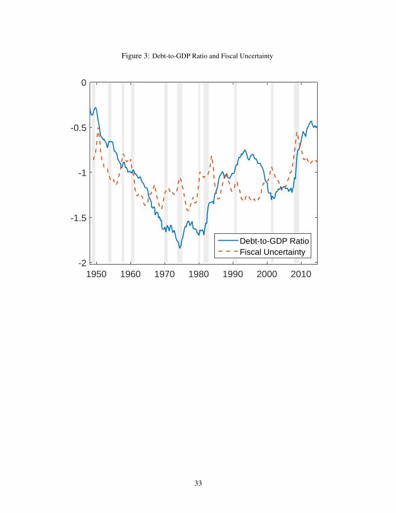
Figure 3: Debt-to-GDP Ratio and Fiscal Uncertainty

1950 1960 1970 1980 1990 2000 2010-2

-1.5

-1

-0.5

0

Debt-to-GDP RatioFiscal Uncertainty

33

Figure 4: Impulse Response Functions to a 1 s.d. Tax Shock

5 10 15 20

#10-4

-6

-4

-2

0V

5 10 15 20

#10-3

-1.5

-1

-0.5

0"n

5 10 15 20

#10-3

-5

0

5

10"c

5 10 15 200

0.1

0.2

0.3M

5 10 15 20-0.02

-0.015

-0.01

-0.005

0rm

5 10 15 20

#10-3

-5

0

5

10

15rb

34

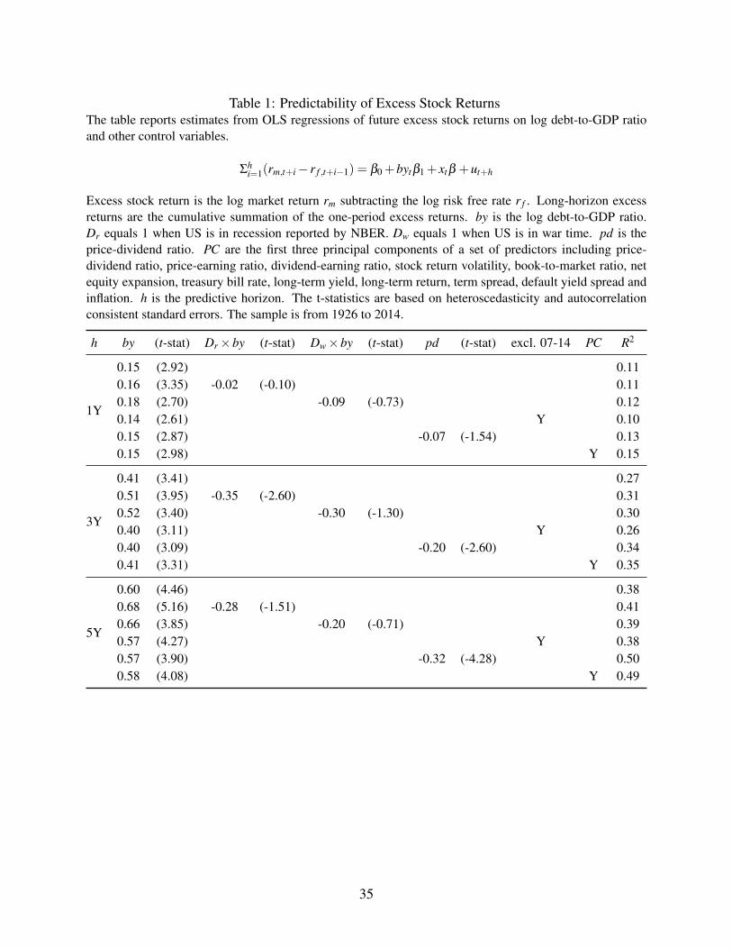
Table 1: Predictability of Excess Stock ReturnsThe table reports estimates from OLS regressions of future excess stock returns on log debt-to-GDP ratioand other control variables.

Σhi=1(rm,t+i− r f ,t+i−1) = β0 +bytβ1 + xtβ +ut+h

Excess stock return is the log market return rm subtracting the log risk free rate r f . Long-horizon excessreturns are the cumulative summation of the one-period excess returns. by is the log debt-to-GDP ratio.Dr equals 1 when US is in recession reported by NBER. Dw equals 1 when US is in war time. pd is theprice-dividend ratio. PC are the first three principal components of a set of predictors including price-dividend ratio, price-earning ratio, dividend-earning ratio, stock return volatility, book-to-market ratio, netequity expansion, treasury bill rate, long-term yield, long-term return, term spread, default yield spread andinflation. h is the predictive horizon. The t-statistics are based on heteroscedasticity and autocorrelationconsistent standard errors. The sample is from 1926 to 2014.

h by (t-stat) Dr×by (t-stat) Dw×by (t-stat) pd (t-stat) excl. 07-14 PC R2

1Y

0.15 (2.92) 0.110.16 (3.35) -0.02 (-0.10) 0.110.18 (2.70) -0.09 (-0.73) 0.120.14 (2.61) Y 0.100.15 (2.87) -0.07 (-1.54) 0.130.15 (2.98) Y 0.15

3Y

0.41 (3.41) 0.270.51 (3.95) -0.35 (-2.60) 0.310.52 (3.40) -0.30 (-1.30) 0.300.40 (3.11) Y 0.260.40 (3.09) -0.20 (-2.60) 0.340.41 (3.31) Y 0.35

5Y

0.60 (4.46) 0.380.68 (5.16) -0.28 (-1.51) 0.410.66 (3.85) -0.20 (-0.71) 0.390.57 (4.27) Y 0.380.57 (3.90) -0.32 (-4.28) 0.500.58 (4.08) Y 0.49

35

Table 2: Predictability of Excess Stock ReturnsThe table reports estimates from OLS regressions of future excess stock returns on log debt-to-GDP ratioand other control variables.

Σhi=1(rm,t+i− r f ,t+i−1) = β0 +bytβ1 + xtβ +ut+h

Excess stock return is the log market return rm subtracting the log risk-free rate r f . Long-horizon excessreturns are the cumulative summation of the one-period excess returns. by is the log debt-to-GDP ratio. Dr

equals 1 when US is in recession reported by NBER. pd is the price-dividend ratio. PC are the first threeprincipal components of a set of predictors including price-dividend ratio, price-earning ratio, dividend-earning ratio, stock return volatility, book-to-market ratio, net equity expansion, treasury bill rate, long-termyield, long-term return, term spread, default yield spread, inflation, investment-capital ratio, consumption-wealth ratio, GDP gap and government investment-capital ratio. liqs is the spread between general col-lateral repo and 3-month T-bill rate. ats is the spread between Moody’s AAA bond and 30-year Treasurybond yield. h is the predictive horizon. The t-statistics are based on heteroscedasticity and autocorrelationconsistent standard errors. The sample is from 1947:I to 2014:IV.

h by (t-stat) Dr×by (t-stat) pd (t-stat) PC liqs (t-stat) ats (t-stat) R2

1Q

0.04 (3.26) 0.040.04 (4.11) -0.01 (-0.26) 0.040.04 (3.30) -0.02 (-2.30) 0.060.06 (3.94) Y 0.080.04 (2.99) 0.70 (0.35) 0.38 (0.30) 0.03

1Y

0.15 (3.78) 0.120.17 (4.38) -0.03 (-0.49) 0.170.15 (3.75) -0.10 (-2.79) 0.200.21 (4.45) Y 0.220.17 (4.03) 4.60 (1.25) -0.44 (-0.13) 0.12

3Y

0.41 (6.59) 0.330.46 (6.74) -0.14 (-1.65) 0.400.40 (5.94) -0.26 (-3.22) 0.490.50 (6.14) Y 0.480.35 (4.98) 6.74 (1.49) -13.87 (-2.30) 0.37

5Y

0.61 (5.11) 0.420.67 (5.76) -0.18 (-1.74) 0.490.56 (5.92) -0.40 (-6.20) 0.660.61 (4.71) Y 0.590.57 (4.80) 12.14 (2.06) -12.10 (-1.80) 0.44

36

Table 3: Out-of-sample TestThe table reports in-sample and out-of-sample R2 from OLS regressions of future excess stock returns onlog debt-to-GDP ratio and other control variables.

Σhi=1(rm,t+i− r f ,t+i−1) = β0 +bytβ1 + x′tβ +ut+h

Excess stock return is the log market return rm subtracting the log risk-free rate r f . Long-horizon excessreturns are the cumulative summation of the one-period excess returns. by is the log debt-to-GDP ratio.The other regressors are as follows: price-dividend ratio (pd), price-earning ratio (pe), dividend-earningratio (de), stock return volatility (svar), book-to-market ratio (bm), net equity expoansion (ntis), treasurybill rate (tbl), long-term yield (lty), long-term return (ltr), term spread (tms), default yield spread (dfy) andinflation (infl). The first column shows the regressor. The out-of-sample period starts in 20 periods from thebeginning of the sample. R2

OS is from univariate regressions and R2OS,by is from bi-variate regression with

debt-to-GDP ratio and a regressor. Column “p” shows p value of testing hypothesis H0 : MSE1 > MSE0against H1 : MSE1 < MSE0. In the row of “by”, MSE0 is the mean squared error from historical mean.MSE1 is the mean squared error from predictive model with by. In other rows, MSE0 is the mean squarederror from a predictor. MSE1 is the mean squared error from predictive model with the predictor and by.The sample is from 1926 to 2014.

R2OS R2

OS,by p R2OS R2

OS,by p R2OS R2

OS,by p

1Y 3Y 5Y

by 0.10 0.00 0.29 0.00 0.29 0.00pd 0.00 0.10 0.00 -0.27 -0.08 0.00 -0.32 -0.14 0.00dy -0.16 -0.02 0.00 -0.73 -0.38 0.00 -0.25 0.20 0.00pe 0.00 0.10 0.00 -0.05 0.30 0.00 -0.16 0.36 0.00de -0.04 0.07 0.01 -0.20 0.10 0.00 -0.12 0.03 0.01

svar -0.05 0.07 0.00 -0.09 0.22 0.00 -0.20 0.06 0.00bm -0.07 0.11 0.00 -0.55 0.06 0.00 -0.56 0.21 0.00ntis -0.10 0.02 0.00 -0.27 0.11 0.00 -0.25 0.23 0.00tbl -0.04 0.04 0.00 -0.52 0.12 0.00 -1.00 0.06 0.00lty -0.06 0.01 0.00 -0.28 0.27 0.00 -1.24 0.35 0.00ltr -0.07 0.06 0.00 -0.05 0.27 0.00 -0.16 0.21 0.00tms -0.01 0.07 0.00 -0.35 0.02 0.00 -0.31 0.12 0.00d f y -0.01 0.10 0.00 -0.16 0.10 0.00 -0.19 0.10 0.00in f l -0.07 0.06 0.01 -0.07 0.25 0.00 -0.11 0.20 0.00

37

Table 4: Out-of-sample TestThe table reports in-sample and out-of-sample R2 from OLS regressions of future excess stock returns onlog debt-to-GDP ratio and other control variables.

Σhi=1(rm,t+i− r f ,t+i−1) = β0 +bytβ1 + x′tβ +ut+h

Excess stock return is the log market return rm subtracting the log risk-free rate r f . Long-horizon excessreturns are the cumulative summation of the one-period excess returns. by is the log debt-to-GDP ratio.The other regressors are as follows: price-dividend ratio (pd), price-earning ratio (pe), dividend-earningratio (de), stock return volatility (svar), book-to-market ratio (bm), net equity expoansion (ntis), treasury billrate (tbl), long-term yield (lty), long-term return (ltr), term spread (tms), default yield spread (dfy), inflation(infl), investment-capital ratio (ik), consumption-wealth ratio (cay), GDP gap (gap), government investment-capital ratio (gik). The first column shows the regressor. The out-of-sample period starts in 20 periods fromthe beginning of the sample. R2

OS is from univariate regressions and R2OS,by is from bi-variate regression with

debt-to-GDP ratio and a regressor. Column “p” shows p value of testing hypothesis H0 : MSE1 > MSE0against H1 : MSE1 < MSE0. In the row of “by”, MSE0 is the mean squared error from historical mean.MSE1 is the mean squared error from predictive model with by. In other rows, MSE0 is the mean squarederror from a predictor. MSE1 is the mean squared error from predictive model with the predictor and by.The sample is from 1947:I to 2014:IV.

R2OS R2

OS,by p R2OS R2

OS,by p R2OS R2

OS,by p R2OS R2

OS,by p

1Q 1Y 3Y 5Y

by 0.02 0.02 0.06 0.02 0.27 0.00 0.34 0.01pd -0.01 0.01 0.02 -0.05 -0.01 0.01 0.01 0.32 0.00 0.10 0.55 0.00dy 0.00 0.02 0.01 -0.02 0.03 0.01 0.01 0.30 0.00 0.11 0.55 0.00pe -0.01 0.00 0.04 -0.07 0.00 0.00 -0.08 0.31 0.00 -0.12 0.43 0.01de -0.02 0.00 0.01 -0.06 -0.01 0.02 -0.13 0.11 0.00 -0.12 0.22 0.01

svar -0.01 0.01 0.02 -0.05 0.02 0.00 -0.16 0.23 0.00 -0.23 0.27 0.01bm -0.02 0.01 0.02 -0.07 0.05 0.00 -0.27 0.24 0.00 -0.49 0.48 0.02ntis -0.03 0.00 0.02 -0.07 -0.01 0.01 -0.18 0.18 0.00 -0.31 0.28 0.01tbl -0.01 0.00 0.02 -0.05 -0.07 0.08 -0.31 0.05 0.03 -0.79 0.29 0.04lty -0.02 -0.02 0.05 -0.14 -0.11 0.00 -0.45 0.18 0.01 -1.24 0.22 0.04ltr -0.02 0.01 0.02 -0.01 0.07 0.00 -0.09 0.26 0.00 -0.14 0.35 0.01tms -0.02 0.00 0.02 -0.07 -0.10 0.16 -0.10 0.24 0.00 -0.31 0.34 0.01d f y -0.02 0.00 0.01 -0.06 0.00 0.00 -0.28 0.03 0.00 -0.46 0.41 0.00in f l 0.00 0.01 0.03 0.02 0.05 0.02 -0.05 0.26 0.00 -0.17 0.36 0.01ik 0.02 0.02 0.22 0.05 0.05 0.09 0.15 0.26 0.01 0.07 0.40 0.02

cay 0.00 -0.01 0.05 0.03 -0.02 0.06 0.09 0.20 0.01 0.15 0.28 0.04gap 0.02 0.04 0.01 0.02 0.10 0.00 0.04 0.36 0.00 0.00 0.46 0.00gik -0.01 0.01 0.01 -0.02 -0.01 0.06 0.03 0.26 0.00 -0.05 0.30 0.00

38

Table 5: Predictability of Corporate Bond Excess ReturnThe table reports estimates from OLS regressions of future excess corporate bond returns on log debt-to-GDP ratio and other control variables.

Σhi=1(rcorp,t+i− r f ,t+i−1) = β0 +β1byt +β2 pdt +β3rvolt +ut+h

Excess corporate bond return is the log Barclay’s corporate bond portfolio return rcorp subtracting the logrisk free rate r f . Longer horizon excess returns are the cumulative summation of the one-period excessreturns. byt is the log debt-to-GDP ratio. by is the log debt to GDP ratio. pd is the log price-dividendratio. svar is the stock return realized volatility. h is the predictive horizon. The corporate bond portfoliois indicated in the name of the panel. The t-statistics are based on heteroscedasticity and autocorrelationconsistent standard errors. The sample is from 1973:I to 2014:IV for investment-grade bond and from1983:I to 2014:IV for high-yield bond.

h by (t-stat) pd (t-stat) svar (t-stat) R2

Investment Grade

1q 0.03 (3.08) -0.01 (-1.72) 0.01 (2.06) 0.061y 0.09 (2.73) -0.04 (-1.42) 0.02 (2.62) 0.132y 0.12 (2.29) -0.04 (-0.91) 0.06 (3.85) 0.20

High Yield

1q 0.04 (3.16) -0.03 (-2.36) 0.01 (1.40) 0.101y 0.12 (2.59) -0.11 (-2.75) 0.04 (1.80) 0.242y 0.13 (1.55) -0.18 (-2.07) 0.07 (2.03) 0.28

39

Table 6: Yield Spreads and Debt-to-GDP ratioThe table reports estimates from OLS regressions of yield spreads on log debt-to-GDP ratio and other controlvariables.

spreadt = β0 +β1byt +β3rvolt +β3tmst +ut

∆spreadt = β0 +β1∆byt +β3∆rvolt +β3∆tmst +ut

The spreads include: Gilchrist and Zakrajsek (2012) spread index (GZ spread), the spreads between Moody’sAaa, Aa, A, Baa bond yield and 30-year treasury bond yield, the spread between general collateral repo rate(Repo), Certificate of Deposits rate (CD) , AA commercial paper (Paper) rate, federal funds rate (FFR) andtreasury bill rate. by is the log debt-to-GDP ratio. svar is the stock return realized volatility. tms is thespread between 10-year treasury bond and 3-month T-bill. Panel A shows the regression in level and PanelB shows the regression in first difference. The t-statistics are based on heteroscedasticity and autocorrelationconsistent standard errors.

h by (t-stat) R2 by (t-stat) svar (t-stat) tms (t-stat) R2

A. Level

GZ spread 0.83 (1.80) 0.10 0.72 (3.92) 0.85 (3.59) 7.97 (1.14) 0.59Aaa-Treasury 0.16 (1.25) 0.03 0.24 (1.75) 0.28 (5.72) -3.73 (-1.26) 0.41Aa-Treasury -0.03 (-0.15) 0.00 -0.02 (-0.09) 0.34 (5.44) -0.35 (-0.10) 0.39A-Treasury -0.21 (-0.70) 0.02 -0.25 (-1.02) 0.40 (4.99) 3.41 (0.69) 0.35

Baa-Treasury -0.19 (-0.52) 0.01 -0.28 (-1.02) 0.52 (3.90) 6.04 (1.04) 0.38Baa-Aaa -0.36 (-1.22) 0.08 -0.52 (-2.17) 0.23 (2.14) 9.79 (2.17) 0.29Repo-Bill -0.83 (-3.84) 0.31 -0.59 (-3.04) 0.10 (1.44) -13.80 (-3.29) 0.42CD-Bill -0.87 (-3.69) 0.18 -0.81 (-3.11) 0.29 (2.98) -2.52 (-0.35) 0.28

Paper-Bill -1.10 (-3.78) 0.29 -0.71 (-2.73) 0.09 (1.47) -22.45 (-3.59) 0.43FFR-Bill -0.79 (-3.86) 0.26 -0.59 (-3.11) 0.11 (1.62) -11.24 (-2.55) 0.35

B. First Difference

GZ spread 3.00 (1.73) 0.06 2.18 (1.51) 0.32 (2.81) -5.77 (-2.22) 0.33Aaa-Treasury 1.55 (2.56) 0.04 1.15 (2.18) 0.18 (5.37) -10.83 (-3.31) 0.35Aa-Treasury 2.06 (2.82) 0.06 1.60 (2.26) 0.20 (4.75) -9.06 (-2.25) 0.33A-Treasury 2.56 (2.56) 0.07 2.00 (2.09) 0.23 (4.27) -7.83 (-2.16) 0.30

Baa-Treasury 3.65 (2.58) 0.09 2.98 (2.18) 0.27 (3.65) -7.90 (-1.45) 0.28Baa-Aaa 2.10 (2.20) 0.08 1.83 (1.90) 0.10 (1.75) 2.91 (1.11) 0.14Repo-Bill -3.43 (-2.85) 0.07 -3.71 (-2.92) 0.13 (2.21) -9.31 (-1.02) 0.15CD-Bill 1.21 (0.52) 0.00 0.10 (0.05) 0.31 (4.01) 35.23 (2.19) 0.20

Paper-Bill -1.58 (-1.13) 0.01 -1.50 (-0.80) 0.02 (0.17) -17.72 (-1.18) 0.08FFR-Bill -3.43 (-2.55) 0.06 -3.75 (-2.69) 0.14 (1.77) -6.86 (-0.74) 0.12

40

Table 7: Risk-free Rate and Debt-to-GDP RatioThe table reports estimates from OLS regressions of real risk-free rate on log debt-to-GDP ratio and othercontrol variables.

r f ,t = β0 +β1byt +β2∆ct +β3∆ct−1 +β4πt +β5πt−1 +β6 pdt +ut

The real risk-free rate is the nominal risk-free rate minus the four-quarter moving average of past inflation.The first column shows 3-month and 1-month real risk-free rate. “r f , survey” calculate the real risk-freerate using Livingston survey on inflation. by is log debt-to-GDP ratio. ∆c is consumption growth. π isinflation. pd is price-dividend ratio. “r f , survey” is observed bi-annually. The t-statistics are based onheteroscedasticity and autocorrelation consistent standard errors.

Period byt ∆ct ∆ct−1 πt πt−1 pdt R2

1947:I–2014:IV

r f , 3M -0.03 0.39 0.32 -0.76 -0.86 0.00 0.33(-2.94) (2.29) (1.37) (-2.56) (-2.86) (-0.32)

r f , 1M -0.03 0.42 0.32 -0.78 -0.88 0.00 0.35(-3.09) (2.60) (1.45) (-2.74) (-3.14) (-0.21)

r f , survey -0.02 0.02 0.00 -0.22 -0.78 -0.01 0.24(-2.45) (0.07) (-0.01) (-0.99) (-2.12) (-1.17)

1926–2014r f , 3M -0.05 0.01 -0.09 -0.79 0.19 0.00 0.71

(-4.97) (0.12) (-0.71) (-8.09) (1.69) (0.21)

41

Table 8: Government Debt Return and Debt-to-GDP RatioPanel A reports estimates from OLS regressions of government debt return on log debt-to-GDP ratio.

Σhi=1rb,t+i = β0 +β1byt +u+h

The government debt return rb is the log average return across terms to maturity on all the governmentdebt outstanding subtracting the realized inflation. Longer horizon returns are the cumulative summationof the one-period return. by is log debt-to-GDP ratio. The t-statistics are based on heteroscedasticity andautocorrelation consistent standard errors. The sample is from 1929 to 2014.Panel B reports the variance decomposition. Surplus is Et [Σ j=0κ

j1(κ2τyt+ j − κ3gyt+ j)]. Growth is

Et [Σ j=0κj

1∆yt+ j]. Return is Et [Σ j=0κj

1rb,t+ j]. The conditional expectation is computed from a first ordervector autoregression model with five variables [byt , gyt , τyt , ∆yt , rb,t ]

′.

A. Predictive Regression

h byt (t-stat) R2

1Y -0.04 (-2.29) 0.095Y -0.14 (-1.74) 0.15

10Y -0.24 (-2.00) 0.1720Y -0.44 (-3.59) 0.28

B. Variance Decomposition

surplus growth discount ratecov(byt ,Et [.])/var(byt) 0.49 0.30 -0.25

42

Table 9: Fiscal Uncertainty and Debt-to-GDP RatioThis table reports the correlation between log debt-to-GDP ratio and measures of uncertainty. Panel A showsthe broad-based measure of fiscal and macro uncertainty. Panel B shows the Economic Policy UncertaintyIndex from Baker et al. (2015).

corr(by, uncertainty)1947:I–2014:IV 1985:I:2014:IV

A. Broad-based Uncertainty Measure

1Y Fiscal Uncertainty 0.28 0.213Y Fiscal Uncertainty 0.50 0.295Y Fiscal Uncertainty 0.54 0.291Y Macro Uncertainty 0.06 0.153Y Macro Uncertainty 0.06 0.065Y Macro Uncertainty 0.06 -0.26

B. Economic Policy Uncertainty

Economic Policy Uncertainty 0.26Monetary policy -0.18

Fiscal Policy 0.36Taxes 0.33

Government spending 0.37Health care 0.58

National security -0.14Entitlement programs 0.45

Regulation 0.51Financial Regulation 0.27

Trade policy -0.01Sovereign debt, currency crises 0.31

43

Table 10: Fiscal Uncertainty and Asset PricesPanel A reports estimates from OLS regressions of asset prices on log debt-to-GDP ratio.

rt = β0 +β1Uncertaintyt +ut

Excess stock return is the log market return rm subtracting the log risk-free rate r f . by is the logdebt-to-GDP ratio. Excess corporate bond return is the log Barclay’s corporate investment-grade bondportfolio return rcorp subtracting the log risk free rate r f . GZ spread is the credit spread in Gilchrist andZakrajsek (2012). The real risk free rate r f is the nominal risk free rate minus the four-month movingaverage of past inflation. The government debt return rb is the log average return across terms to maturityon all the government debt outstanding subtracting the realized inflation. Uncertainty is measured as thebroad-based 3-year fiscal uncertainty or the fiscal policy uncertainty in Economic Policy Uncertainty Indexfrom Baker et al. (2015).

Broad-based (t-stat) R2 EPU (t-stat) R2

rm,t+1− r f ,t , 1Y 0.021 (1.26) 0.02 0.048 (2.39) 0.08rm,t+1− r f ,t , 3Y 0.073 (2.14) 0.07 0.153 (2.99) 0.25rm,t+1− r f ,t , 5Y 0.168 (2.93) 0.21 0.188 (4.79) 0.24

rcorp,t+1− r f ,t , 1Y 0.025 (2.43) 0.07 0.018 (2.42) 0.09GZ spread 0.007 (2.51) 0.43 0.003 (1.10) 0.06

r f ,t -0.002 (-1.54) 0.09 -0.002 (-2.19) 0.10rb,t+1 -0.002 (-0.41) 0.00 -0.012 (-1.99) 0.09

44

Table 11: CalibrationThe table reports the calibration of the model. Panel A contains the preferences and technology paraemters.Panel B contains fiscal policy parameters. Panel C contains parameters in fiscal consolidation and govern-ment spending policies.

.

Description Parameter Value

A. Preferences and Technology

Subject discount factor β 0.994Intertemporal elasticity of substitution ψ 2

Relative risk aversion γ 10Capital share α 0.33

Intermediate inputs share ξ 0.50Depreciation rate of R&D capital φ 0.075

Depreciation rate of capital δ 0.025Investment adjustment cost ξk 0.80

Exogenous productivity shock volatility σa 0.008Exogenous productivity persistence ρ 0.97

B. Fiscal Policy

Corporatetax rate mean µτc 0.36Corporate tax rate shock volatility στ.0/

√1−ρτ 0.03

Corporate tax rate persistence ρτ 0.99Fiscal uncertainty shock volatility στ,w 0.7

Fiscal uncertainty persistence ντ 0.995G-Y ratio mean µgy 0.17

Labor tax rate mean µτl 0.10Long-term debt maturity φb 0.99Bond quantity persistence ρb 0.99Bond quantity volatility σb 0.01

C. Fiscal Consolidation and Government Spending Policy

Fiscal consolidation φτ 0.001Fiscal consolidation volatility σ2

φτ0.006

Fiscal consolidation cyclicality corr(φτ,t+1,εt+1) -0.5G-Y ratio shock volatility σg,0/

√1−ρg 0.01

G-Y ratio persistence ρg 0.99

45

Table 12: Macroeconomic Dynamics and Asset PricesThe table reports the macroeconomic and asset price moments in the data and the model. The reportedmodel moments are the mean, 5% and 95% quantile of short-sample simulations. The simulated sampleperiod is 85 years.

Data Model 5% 95%

E[∆y] 1.80 1.80 -0.40 3.59

σ(∆y) 5.00 2.80 2.55 3.15

σ(∆c) 2.70 2.62 1.82 4.16

E[rm− r f ] 5.59 5.19 2.34 8.54

σ(rm) 20.04 7.32 5.81 10.12

E[r f ] 0.45 1.48 -0.46 2.98

σ(r f ) 3.75 1.42 0.90 2.28

E[rb] 1.48 0.75 -1.86 0.59

σ(rb) 5.31 4.54 3.69 5.96

E[pd] 3.39 3.63 3.01 4.16

σ(pd) 0.45 0.43 0.24 0.74

E[B/Y ] 0.40 0.52 0.41 0.63

σ(B/Y ) 0.18 0.08 0.05 0.12

E[T/Y ] 0.20 0.20 0.19 0.21

σ(T/Y ) 0.02 0.01 0.00 0.02

46

Table 13: Asset Prices, Debt-to-GDP and Fiscal UncertaintyPanel A reports estimates from OLS regressions of asset prices on log debt-to-GDP ratio.

rt = β0 +β1byt +ut

Excess stock return is the log market return rm subtracting the log risk free rate r f . by is the logdebt-to-GDP ratio. The real risk-free rate r f is the nominal risk-free rate minus the four-quarter movingaverage of past inflation. The government debt return rb is the log average return across terms to maturityon all the government debt outstanding subtracting the realized inflation. The standard errors areheteroscedasticity and autocorrelation consistent. Panel B reports estimates from OLS regressions of assetprices on the broad-based 3-year fiscal uncertainty. Model is from the benchmark calibration. The reportedmodel moments are the mean, 5% and 95% quantile of β and R2 in short-sample simulations. Thesimulated sample period is 85 years.

Data Modelβ s.e. R2 β 5% 95% R2 5% 95%

A. Debt-to-GDP ratio

rm,t+1− r f ,t , 1Q 0.04 (0.01) 0.04 0.04 -0.02 0.10 0.01 0.00 0.03rm,t+1− r f ,t , 1Y 0.15 (0.05) 0.11 0.15 -0.07 0.40 0.04 0.00 0.13rm,t+1− r f ,t , 3Y 0.41 (0.12) 0.27 0.43 -0.20 1.14 0.10 0.00 0.31rm,t+1− r f ,t , 5Y 0.60 (0.13) 0.38 0.65 -0.41 1.76 0.14 0.00 0.45

r f ,t -0.04 (0.02) 0.21 -0.09 -0.19 0.01 0.27 0.01 0.65rb,t+1 -0.04 (0.02) 0.09 -0.18 -0.35 -0.03 0.10 0.00 0.26

rb,t+1, 10Y -0.24 (0.12) 0.17 -1.18 -2.43 0.10 0.33 0.01 0.77

rm,t+1, 1Y 0.11 (0.05) 0.05 0.06 -0.17 0.35 0.02 0.00 0.08rm,t+1, 3Y 0.29 (0.12) 0.15 0.06 -0.19 0.33 0.02 0.00 0.09rm,t+1, 5Y 0.43 (0.15) 0.22 0.30 -0.95 1.60 0.08 0.00 0.29

B. Fiscal Uncertainty

corr(by,uncertainty) 0.50 0.43 -0.15 0.86

rm,t+1− r f ,t , 1Y 0.02 (0.02) 0.02 0.02 0.01 0.03 0.08 0.00 0.18rm,t+1− r f ,t , 5Y 0.17 (0.05) 0.21 0.09 0.03 0.17 0.30 0.03 0.59

r f ,t -0.002 (0.001) 0.09 -0.01 -0.01 0.00 0.19 0.00 0.53rb,t+1 -0.002 (0.01) 0.00 -0.01 -0.02 -0.01 0.11 0.03 0.23

47

Table 14: Mechanisms of Fiscal UncertaintyPanel A reports estimates from OLS regressions of asset prices on log debt-to-GDP ratio.

rt = β0 +β1byt +ut

Excess stock return is the log market return rm subtracting the log risk free rate r f . by is the logdebt-to-GDP ratio. The real risk-free rate r f is the nominal risk-free rate minus the four-quarter movingaverage of past inflation. The government debt return rb is the log average return across terms to maturityon all the government debt outstanding subtracting the realized inflation. The standard errors areheteroscedasticity and autocorrelation consistent. Panel B reports estimates from OLS regressions of assetprices on the broad-based 3-year fiscal uncertainty.

“Tax Vol” is the benchmark calibration that has stochastic volatility. “Vol and Cons” includes both stochasticvolatility and uncertain fiscal consolidations. “Cons.” has uncertain fiscal consolidations but no stochasticvolatility. “Spending” introduce spending shocks in the benchmark. “No Vol” has no stochastic volatilityand uncertain fiscal consolidations. The reported model moments are the mean of β and R2 in short-samplesimulations. The simulated sample period is 85 years.

Data Tax Vol Vol & Cons. Cons. Spending No Volβ R2 β R2 β R2 β R2 β R2 β R2

A. Debt-to-GDP ratio

rm,t+1− r f ,t , 1Q 0.04 0.04 0.04 0.01 0.05 0.01 0.03 0.01 0.04 0.01 0.01 0.00rm,t+1− r f ,t , 1Y 0.15 0.11 0.15 0.04 0.18 0.05 0.11 0.02 0.15 0.04 0.02 0.01rm,t+1− r f ,t , 3Y 0.41 0.27 0.43 0.10 0.49 0.13 0.30 0.07 0.43 0.10 0.07 0.03rm,t+1− r f ,t , 5Y 0.60 0.38 0.65 0.14 0.75 0.18 0.45 0.10 0.65 0.14 0.10 0.05

r f ,t -0.04 0.21 -0.09 0.27 -0.11 0.38 -0.09 0.32 -0.09 0.27 -0.06 0.16rb,t+1 -0.04 0.09 -0.18 0.10 -0.21 0.14 -0.16 0.10 -0.18 0.10 -0.07 0.04

rb,t+1, 10Y -0.24 0.17 -1.18 0.33 -1.43 0.48 -0.99 0.46 -1.18 0.33 -0.37 0.17

rm,t+1, 1Y 0.11 0.05 0.06 0.02 0.07 0.02 0.01 0.02 0.06 0.02 -0.03 0.02rm,t+1, 3Y 0.29 0.15 0.06 0.02 0.06 0.02 0.02 0.02 0.06 0.02 -0.02 0.02rm,t+1, 5Y 0.43 0.22 0.30 0.08 0.31 0.09 0.10 0.07 0.30 0.08 -0.09 0.07

B. Fiscal Uncertainty

corr(byt ,vart(τc,t+1)) 0.50 0.43 0.38 1.00 0.43 0.00

rm,t+1− r f ,t , 1Y 0.02 0.02 0.02 0.08 0.02 0.06 0.01 0.02 0.02 0.08rm,t+1− r f ,t , 5Y 0.17 0.21 0.09 0.30 0.10 0.26 0.04 0.10 0.09 0.30

r f ,t -0.002 0.09 -0.01 0.19 -0.01 0.18 -0.01 0.32 -0.01 0.19rb,t+1 -0.002 0.00 -0.01 0.11 -0.02 0.08 -0.01 0.10 -0.01 0.11

48

Table 15: Tax Impact on GrowthThe table shows the OLS regressions of economic growth on log tax-to-GDP ratio.

Σhi=1∆yt+i = β0 + τytβ1 +ut+h

The growth ∆y is measured as real output, real private consumption or total factor productivity. τy is thelog tax-to-GDP ratio. Tax is the federal tax receipts. h is the predictive horizon. The standard errors areheteroscedasticity and autocorrelation consistent. The sample is from 1947:I to 2014:IV. The reported modelmoments are the mean, 5% and 95% quantile of β and R2 in short-sample simulations. The simulated sampleperiod is 85 years.

Data Modelh β s.e. R2 β 5% 95% R2 5% 95%

1Youtput, -0.15 (0.04) 0.13 -0.29 -0.62 0.07 0.16 0.00 0.46

consumption -0.09 (0.03) 0.06 -0.41 -0.80 -0.04 0.24 0.01 0.55TFP -0.12 (0.03) 0.16 -0.32 -0.74 0.13 0.11 0.00 0.33

10Youtput -0.66 (0.19) 0.21 -1.43 -4.81 1.85 0.19 0.00 0.55

consumption -0.35 (0.15) 0.09 -2.04 -5.19 1.19 0.26 0.00 0.67TFP -0.32 (0.15) 0.13 -1.31 -5.42 2.96 0.15 0.00 0.47

49

Appendix I. Data

The appendix details the data source.The government debt data are from Dallas Fed, Flow of Funds, and George Hall. Dallas Fed

reports the monthly level of par and market values of gross, non-marketable and net debt from1942 to 2014. Flow of Funds database reports debt held by the Federal Reserve System and rest ofthe world. George Hall kindly provides debt data from 1926 to 1941.

The stock return and predictors are from Amit Goyal’s website. The stock return is the returnon S&P 500 index from CRSP. The risk-free rate is the 3-month T-bill. The price-dividend ratio(pd) is the difference between the log of prices and the log of dividends. The dividend yield (dy)is the difference between the log of dividends and the log of lagged prices. The price-earningratio (pe) is the difference between log of prices and log of earnings. The dividend-earning ratio(d/e) is the difference between log of dividends and log of earnings. Stock return volatility (svar)is the sum of squared daily returns on S&P 500. The book-to-market ratio (bm) is the ratio ofbook value to market value for the Dow Jones Industrial Average. Net equity expansion (ntis) isthe ratio of twelve-month moving sums of net issues by NYSE-listed stocks divided by the totalmarket capitalization of NYSE stocks. Treasury bill rate (tbl) is the 3-month treasury bill rate.Long-term yield (lty) is the long-term government bond yield. Long-term return (ltr) is the long-term government bond return. Term spread (tms) is the difference between the long-term yield ongovernment bonds and the T-bill. Default yield spread (dfy) is the difference between BAA- andAAA- rated corporate bond yields. Inflation (infl) is the CPI inflation. Investment-capital ratio (ik)is the ratio of aggregate (private nonresidential fixed) investment to aggregate capital for the wholeeconomy. Consumption-wealth ratio (cay) is the error correction term calculated from the co-integration of consumption, income, and wealth. Two predictors are constructed separately. GDPgap (gap) is the difference between actual GDP and potential GDP over potential GDP. PotentialGDP is from CBO. Government investment-capital ratio (gik) is the ratio of aggregate governmentinvestment to aggregate government capital.

Investment-grade and high-yield corporate bond return indices are from Barclay’s. Gilchristand Zakrajsek (2012) spread is from Simon Gilchrist’s website. Moody’s Aaa, Aa, A, Baa bondyields are from Bloomberg. 30-year treasury bond yield is from CRSP. General collateral reporate (Repo) combines two series. It is the banker’s acceptance rate from Fred before 1991 and3-month general collateral repo rate from Bloomberg after 1991. Certificate of Deposits rate (CD)and AA commercial paper rate are from Fred. 1-month and 3-month nominal risk-free rates arefrom CRSP. Expected inflation in Livingston survey is from Philly Fed. The average return ongovernment debt is from George Hall.

The data on macroeconomic and fiscal variables are from NIPA. In constructing the fiscal un-certainty measure, I use a large panel of quarterly macroeconomic series from FRED-QD database

A1

(McCracken and Ng, 2016). I include all the series that are available from 1948 in Group 1: NIPA,Group 2: Industrial Production, Group 3: Employment and Unemployment, Group 5: Inventories,Orders, and Sales, Group 6: Prices, Group 7: Earnings and Productivity, and Group 9: Money andCredit. I exclude other groups about financial markets. These result in 132 macroeconomics series.ID shows the series number in the database. TC denotes the data transformation: (1) no transfor-mation; (2) ∆xt ; (3) ∆2xt ; (4)log(xt);(5)∆log(xt);(6)∆2log(xt). (7)∆(xt/xt−1)− 1). The transfor-mation follows McCracken and Ng (2016). I augment the database with 37 fiscal-policy-relatedseries from NIPA Table 3.2, 3.3, 3.9.5, and 3.10.5. These variables cover the major components ofgovernment receipts, consumption, investment, and transfer in the federal and state and local level.I take the ratio between the fiscal variables and nominal GDP and take the log difference.

Fiscal Policy Variables Federal State and Local

Current receipts 3.2 3.3Current tax receipts 3.2 3.3

Personal current taxes 3.2 3.3Taxes on production and imports 3.2 3.3Taxes on corporate income 3.2 3.3

Contributions for government social insurance 3.2Current transfer receipts 3.2

Capital transfer receipts 3.2 3.3Current expenditures 3.2 3.3

Consumption expenditures 3.2 3.3Compensation of general government employees 3.10.5 3.10.5Consumption of general government fixed capital 3.10.5 3.10.5Durable goods 3.10.5Nondurable goods 3.10.5Services 3.10.5

Current transfer payments 3.2 3.3Interest payments 3.2 3.3Subsidies 3.2Gross investment 3.9.5 3.9.5

Structures 3.9.5Equipment 3.9.5Intellectual property products 3.9.5

National defense consumption expenditures and gross investment 3.9.5Nondefense consumption expenditures and gross investment 3.9.5

A2

ID TC FRED MNEMONIC DESCRIPTION

1. NIPA

1 5 GDPC96 Real Gross Domestic Product, 3 Decimal

2 5 PCECC96 Real Personal Consumption Expenditures

3 5 PCDG Personal Consumption Expenditures: Durable Goods

4 5 PCESV Personal Consumption Expenditures: Services

5 5 PCND Personal Consumption Expenditures: Nondurable Goods

6 5 GPDIC96 Real Gross Private Domestic Investment, 3 decimal

7 5 FPI Fixed Private Investment

8 5 Y033RC1Q027SBEA Gross Private Domestic Investment: Fixed Investment: Nonresidential: Equipment

9 5 PNFI Private Nonresidential Fixed Investment

10 5 PRFI Private Residential Fixed Investment

11 1 A014RE1Q156NBEA Shares of gross domestic product: Gross private domestic investment: Change in private inventories

16 5 EXPGSC96 Real Exports of Goods and Services, 3 Decimal

17 5 IMPGSC96 Real Imports of Goods and Services, 3 Decimal

18 5 DPIC96 Real Disposable Personal Income

19 5 OUTNFB Nonfarm Business Sector: Real Output

20 5 OUTBS Business Sector: Real Output

194 2 B020RE1Q156NBEA Shares of gross domestic product: Exports of goods and services

195 2 B021RE1Q156NBEA Shares of gross domestic product: Imports of goods and services

2. Industrial Production

22 5 INDPRO Industrial Production Index

23 5 IPFINAL Industrial Production: Final Products (Market Group)

24 5 IPCONGD Industrial Production: Consumer Goods

25 5 IPMAT Industrial Production: Materials

26 5 IPDMAT Industrial Production: Durable Materials

28 5 IPDCONGD Industrial Production: Durable Consumer Goods

29 5 IPB51110SQ Industrial Production: Durable Goods: Automotive products

30 5 IPNCONGD Industrial Production: Nondurable Consumer Goods

31 5 IPBUSEQ Industrial Production: Business Equipment

34 1 CUMFNS Capacity Utilization: Manufacturing (SIC)

198 5 IPMANSICS Industrial Production: Manufacturing (SIC)

201 1 NAPMPI ISM Manufacturing: Production Index

205 1 NAPM ISM Manufacturing: PMI Composite Index

A3

ID TC FRED MNEMONIC DESCRIPTION

3. Employment and Unemployment

35 5 PAYEMS All Employees: Total Nonfarm Payrolls36 5 USPRIV All Employees: Total Private Industries37 5 MANEMP All Employees: Manufacturing38 5 SRVPRD All Employees: Service-Providing Industries39 5 USGOOD All Employees: Goods-Producing Industries40 5 DMANEMP All Employees: Durable goods41 5 NDMANEMP All Employees: Nondurable goods42 5 USCONS All Employees: Construction43 5 USEHS All Employees: Education and Health Services44 5 USFIRE All Employees: Financial Activities45 5 USINFO All Employees: Information Services46 5 USPBS All Employees: Professional and Business Services47 5 USLAH All Employees: Leisure and Hospitality48 5 USSERV All Employees: Other Services49 5 USMINE All Employees: Mining and logging50 5 USTPU All Employees: Trade, Transportation and Utilities51 5 USGOVT All Employees: Government52 5 USTRADE All Employees: Retail Trade53 5 USWTRADE All Employees: Wholesale Trade54 5 CES9091000001 All Employees: Government: Federal57 5 CE16OV Civilian Employment58 2 CIVPART Civilian Labor Force Participation Rate59 2 UNRATE Civilian Unemployment Rate60 2 LNS13008397 Of Total Unemployed, Percent Unemployed Less than 5 Weeks61 2 LNS13025703 Of Total Unemployed, Percent Unemployed 27 Weeks and over62 2 LNS14000012 Unemployment Rate: 16 to 19 years63 2 LNS14000025 Unemployment Rate: 20 years and over, Men64 2 LNS14000026 Unemployment Rate: 20 years and over, Women65 5 UEMPLT5 Number of Civilians Unemployed for Less Than 5 Weeks66 5 UEMP5TO14 Number of Civilians Unemployed for 5 to 14 Weeks67 5 UEMP15T26 Number of Civilians Unemployed for 15 to 26 Weeks68 5 UEMP27OV Number of Civilians Unemployed for 27 Weeks and Over74 5 HOABS Business Sector: Hours of All Persons76 5 HOANBS Nonfarm Business Sector: Hours of All Persons77 1 AWHMAN Average Weekly Hours of Production and Nonsupervisory Employees: Manufacturing202 2 UEMPMEAN Average (Mean) Duration of Unemployment203 2 CES0600000007 Average Weekly Hours of Production and Nonsupervisory Employees: Goods-Producing204 1 NAPMEI ISM Manufacturing: Employment Index

5: Inventories, Orders, and Sales

94 1 NAPMSDI ISM Manufacturing: Supplier Deliveries Index206 1 NAPMNOI ISM Manufacturing: New Orders Index207 1 NAPMII ISM Manufacturing: Inventories Index

A4

ID TC FRED MNEMONIC DESCRIPTION

6. Prices

96 6 PCECTPI Personal Consumption Expenditures: Chain-type Price Index

98 6 GDPCTPI Gross Domestic Product: Chain-type Price Index

99 6 GPDICTPI Gross Private Domestic Investment: Chain-type Price Index

100 6 IPDBS Business Sector: Implicit Price Deflator

101 6 DGDSRG3Q086SBEA PCE: Goods (chain-type price index)

102 6 DDURRG3Q086SBEA PCE: Durable goods (chain-type price index)

103 6 DSERRG3Q086SBEA PCE: Services (chain-type price index)

104 6 DNDGRG3Q086SBEA PCE: Nondurable goods (chain-type price index)

105 6 DHCERG3Q086SBEA PCE: Services: Household consumption expenditures (chain-type price index)

106 6 DMOTRG3Q086SBEA PCE: Durable goods: Motor vehicles and parts (chain-type price index)

107 6 DFDHRG3Q086SBEA PCE: Durable goods: Furnishings and durable household equipment (chain-type price index)

108 6 DREQRG3Q086SBEA PCE: Durable goods: Recreational goods and vehicles (chain-type price index)

109 6 DODGRG3Q086SBEA PCE: Durable goods: Other durable goods (chain-type price index)

110 6 DFXARG3Q086SBEA PCE: Nondurable goods: Food and beverages purchased for off-premises consumption

(chain-type price index)

111 6 DCLORG3Q086SBEA PCE: Nondurable goods: Clothing and footwear (chain-type price index)

112 6 DGOERG3Q086SBEA PCE: Nondurable goods: Gasoline and other energy goods (chain-type price index)

113 6 DONGRG3Q086SBEA PCE: Nondurable goods: Other nondurable goods (chain-type price index)

114 6 DHUTRG3Q086SBEA PCE: Services: Housing and utilities (chain-type price index)

115 6 DHLCRG3Q086SBEA PCE: Services: Health care (chain-type price index)

116 6 DTRSRG3Q086SBEA PCE: Transportation services (chain-type price index)

117 6 DRCARG3Q086SBEA PCE: Recreation services (chain-type price index)

118 6 DFSARG3Q086SBEA PCE: Services: Food services and accommodations (chain-type price index)

119 6 DIFSRG3Q086SBEA PCE: Financial services and insurance (chain-type price index)

120 6 DOTSRG3Q086SBEA PCE: Other services (chain-type price index)

121 6 CPIAUCSL Consumer Price Index for All Urban Consumers: All Items

123 6 PPIFGS Producer Price Index by Commodity for Finished Goods

124 6 PPIACO Producer Price Index for All Commodities

125 6 PPIFCG Producer Price Index by Commodity for Finished Consumer Goods

126 6 PPIFCF Producer Price Index by Commodity for Finished Consumer Foods

127 6 PPIIDC Producer Price Index by Commodity Industrial Commodities

128 6 PPIITM Producer Price Index by Commodity Intermediate Materials: Supplies and Components

129 1 NAPMPRI ISM Manufacturing: Prices Index

131 5 WPU0561 Producer Price Index by Commodity for Fuels and Related Products and Power:

Crude Petroleum (Domestic Production)

214 6 PPICRM Producer Price Index by Commodity for Crude Materials for Further Processing

215 6 PPICMM Producer Price Index by Commodity Metals and metal products: Primary nonferrous metals

216 6 CPIAPPSL Consumer Price Index for All Urban Consumers: Apparel

217 6 CPITRNSL Consumer Price Index for All Urban Consumers: Transportation

218 6 CPIMEDSL Consumer Price Index for All Urban Consumers: Medical Care

220 6 CUUR0000SAD Consumer Price Index for All Urban Consumers: Durables

222 6 CPIULFSL Consumer Price Index for All Urban Consumers: All Items Less Food

223 6 CUUR0000SA0L2 Consumer Price Index for All Urban Consumers: All items less shelter

A5

ID TC FRED MNEMONIC DESCRIPTION

7. Earnings and Productivity

134 5 CES2000000008 Average Hourly Earnings of Production and Nonsupervisory Employees: Construction135 5 CES3000000008 Average Hourly Earnings of Production and Nonsupervisory Employees: Manufacturing137 5 COMPRNFB Nonfarm Business Sector: Real Compensation Per Hour138 5 RCPHBS Business Sector: Real Compensation Per Hour140 5 OPHNFB Nonfarm Business Sector: Real Output Per Hour of All Persons141 5 OPHPBS Business Sector: Real Output Per Hour of All Persons142 5 ULCBS Business Sector: Unit Labor Cost144 5 ULCNFB Nonfarm Business Sector: Unit Labor Cost145 5 UNLPNBS Nonfarm Business Sector: Unit Nonlabor Payments225 6 CES0600000008 Average Hourly Earnings of Production and Nonsupervisory Employees: Goods-Producing

9. Money and Credit

162 5 AMBSLREAL Real St. Louis Adjusted Monetary Base167 5 BUSLOANS Commercial and Industrial Loans, All Commercial Banks168 5 CONSUMER Consumer Loans at All Commercial Banks169 5 NONREVSL Total Nonrevolving Credit Owned and Securitized, Outstanding170 5 REALLN Real Estate Loans, All Commercial Banks172 5 TOTALSL Total Consumer Credit Owned and Securitized, Outstanding226 6 DTCOLNVHFNM Consumer Motor Vehicle Loans Owned by Finance Companies, Outstanding227 6 DTCTHFNM Total Consumer Loans and Leases Owned and Securitized by Finance Companies, Outstanding228 6 INVEST Securities in Bank Credit at All Commercial Banks

A6

Appendix II. Robustness

The results in stock return predictability in Section 2.2 are robust across many dimensions. First,I address the high persistence of the debt-to-GDP ratio. I use the efficient test by Campbell andYogo (2006) that corrects for the endogeneity bias (Stambaugh, 1999) and provides an accurate ap-proximation to the finite-sample distribution of test statistics under flexible degrees of persistence(stationary, local-to-unity, and unit root). The results confirm that the predictability is present af-ter considering the persistence of the predictor. Second, in the benchmark case, the governmentdebt is defined as the market value of net debt held by the public. I consider other definitions andcomponents of debt that have different economic interpretations (non-marketable debt, book value,intergovernmental holding, fed holding, foreign holding). The results are similar to the benchmarkcase. Third, I verify the forecasting power using data from UK and Canada who has arguably littledefault risk and stationary debt-to-GDP ratio.

Persistence One key concern is the high persistence of the predictor. The debt-to-GDP ratiohas a persistence of 0.957 at annual frequency. The stationarity of debt-to-GDP ratio is examinedthoroughly in the literature, and there is no convincing evidence of a unit root (Bohn, 2005). If thedebt-to-GDP ratio is nonstationary, with probability one it will implausibly diverge to infinity.

The high persistence of the predictor leads to potential invalidity of the inference in two ways.First, if the innovation to the predictor and innovation to the return are correlated, there is a small-sample bias (Stambaugh, 1999). Second, the high degree of persistence results in a nonstandardasymptotic distribution. I use the efficient test by Campbell and Yogo (2006) to address bothproblems. They propose a Bonferroni test that corrects for the endogeneity and provides an ac-curate approximation to the finite-sample distribution of test statistics under flexible degrees ofpersistence (stationary, local-to-unity, and unit root). In Table A1, the test results confirm thatthe conventional t-test in Table 1 is valid. The 95% confidence interval does not include zero atall horizons and sample periods. The main reason is that the correlation between innovations ofdebt-to-GDP ratio and return ρue is close to zero, while the correlations are very high in a varietyof valuation ratios.

Components of Government Debt In the benchmark case, the government debt is defined asthe market value of net debt held by the public. There are other definitions and components ofdebt that have different economic interpretations. The gross level includes debt held by the gov-ernment accounts that does not represent what the government owes.18 A portion of the debt isnon-marketable and cannot be traded in secondary markets. Given quantitative easing and the

18These accounts include the Social Security Trust Fund, federal employee retirement funds, the UnemploymentTrust Fund, etc.

A7

rapid growth of foreign investors, the debt held by the Federal Reserve System and foreigners areof interest on their own. Moreover, the commonly reported value is the par value not marked tomarket. In comparison, the benchmark definition is a more accurate measure in that net debt ismore relevant than gross debt to measure the indebtedness of the government and market valuereflects up-to-date information in yields changes. Nevertheless, I entertain all the definitions inthe following analysis. The correlations of different debt-to-GDP ratios are around 0.9. TableA2 reports the results. The difference between various definitions is small in that all the coef-ficients are around 0.15, and R2 around 10% at the annual horizon. Results are similar at otherhorizons. Therefore, the different definitions and decomposition of the government debt share thesame forecasting power. As we see, the choice of benchmark is innocuous. In the last row, I definedebt-to-GDP ratio as the ratio of net debt and potential GDP that capture the ideal level of trendGDP without business cycles, measured by Congress Budget Office. The predictability resultsremain in this setting. In fact, the denominator plays the role of normalization.19

International Evidence I verify the forecasting power using data from other countries. I use thedebt-to-GDP ratio of each country to predict the excess return on the country’s MSCI Index. Oneobvious mechanism is that default probability increases with debt-to-GDP ratio, thus affecting theasset prices on all the markets. This sovereign default premium should be of first order in mostcountries. In this paper, I focus on the default-free case and left the interesting default mechanismfor future research. I choose countries that have arguably no default risks. The finding in the USmarket also shows up in Canada and UK in Table A3. The coefficients are statistically significant,and the magnitude is around 0.2, close to 0.15 in the US. In Germany and Japan, the debt-to-GDPratios have a clear upward trend in the sample. So I exclude them from this test. This trendingdebt could be due to country-level heterogeneity. It is clear that a trend does not serve the role of apredictor.

19Debt-to-Consumption ratio and Debt-to-Industrial-Production ratio yield similar results. Therefore, the forecast-ing information is in debt and price instead of the various denominators. Similarly, the price-dividend ratio andprice-earning ratio have similar forecasting power.

A8

Table A1: Bonferroni Test of PredictabilityThe table reports the Bonferroni test of predictability in Campebll and Yogo (2006).

rm,t+1− r f ,t = α +βbyt +ut+1

byt+1 = µ +ρbyt + et+1

Excess stock return is the log market return rm subtracting the log risk-free rate r f . by is the log debt toGDP ratio. h is the predictive horizon. The log debt-to-GDP ratio is modeled as an autoregressive process.The table shows the point estimate β and 95% confidence interval based on the Bonferroni-Q test.ρue = corr(ut+1,et+1).

Period h β 95% CI ρue

1929-20141Y 0.15 [0.06, 0.24] 0.032Y 0.30 [0.09, 0.49] -0.123Y 0.37 [0.12, 0.63] 0.08

1947-20141Q 0.04 [0.02, 0.06] -0.011Y 0.16 [0.06, 0.26] 0.06

A9

Table A2: Predictability of Excess Stock ReturnsThe table reports estimates from OLS regressions of future excess stock returns on log debt-to-GDP ratioand other control variables.

Σhi=1(rm,t+i− r f ,t+i−1) = β0 +bytβ1 + pdtβ2 +ut+h

Excess stock return is the log market return rm subtracting the log risk-free rate r f . Long-horizon excessreturns are the cumulative summation of the one-period excess returns. by is the log debt-to-GDP ratio.The predictive horizon is indicated in the name of the panel. The first column show the component of debtused to construct the debt-to-GDP ratio. The t-statistics are based on heteroscedasticity and autocorrelationconsistent standard errors. The sample is from 1947:I to 2014:IV.

Component of Debt by (t-stat) R2 by (t-stat) R2

1Q 1Y

Net Debt 0.04 (2.89) 0.03 0.14 (3.38) 0.10Gross Debt 0.03 (2.29) 0.02 0.12 (2.74) 0.06Marketable Debt 0.04 (2.77) 0.03 0.15 (3.39) 0.09Net Debt Book Value 0.04 (2.85) 0.03 0.15 (3.40) 0.10Gross Debt Book Value 0.03 (2.26) 0.02 0.13 (2.83) 0.07Marketable Debt Book Value 0.04 (2.75) 0.03 0.16 (3.45) 0.10Net Debt exclud. Fed Holding 0.03 (2.53) 0.03 0.13 (2.97) 0.09Net Debt exclud. Foreign Holding 0.04 (2.89) 0.03 0.14 (2.87) 0.09Net Debt/Potential GDP 0.04 (2.94) 0.03 0.15 (3.53) 0.11

3Y 5Y

Net Debt 0.37 (5.70) 0.30 0.55 (4.57) 0.39Gross Debt 0.33 (3.81) 0.19 0.50 (2.87) 0.25Marketable Debt 0.40 (5.28) 0.25 0.60 (3.67) 0.31Net Debt Book Value 0.40 (5.78) 0.31 0.59 (4.96) 0.40Gross Debt Book Value 0.37 (4.01) 0.20 0.56 (3.14) 0.27Marketable Debt Book Value 0.45 (5.44) 0.27 0.67 (4.01) 0.34Net Debt exclud. Fed Holding 0.33 (4.35) 0.24 0.43 (3.34) 0.28Net Debt exclud. Foreign Holding 0.35 (4.52) 0.25 0.42 (4.20) 0.26Net Debt/Potential GDP 0.38 (4.81) 0.26 0.55 (3.68) 0.34

A10

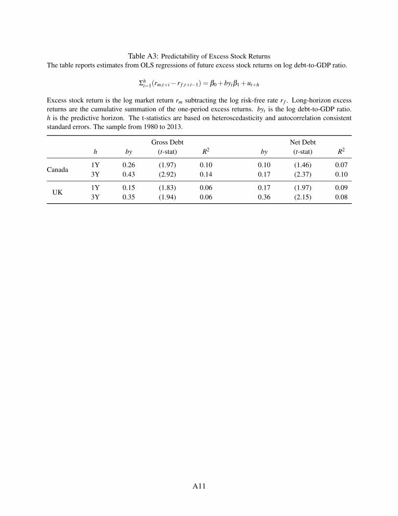
Table A3: Predictability of Excess Stock ReturnsThe table reports estimates from OLS regressions of future excess stock returns on log debt-to-GDP ratio.

Σhi=1(rm,t+i− r f ,t+i−1) = β0 +bytβ1 +ut+h

Excess stock return is the log market return rm subtracting the log risk-free rate r f . Long-horizon excessreturns are the cumulative summation of the one-period excess returns. byt is the log debt-to-GDP ratio.h is the predictive horizon. The t-statistics are based on heteroscedasticity and autocorrelation consistentstandard errors. The sample from 1980 to 2013.

Gross Debt Net Debth by (t-stat) R2 by (t-stat) R2

Canada1Y 0.26 (1.97) 0.10 0.10 (1.46) 0.073Y 0.43 (2.92) 0.14 0.17 (2.37) 0.10

UK1Y 0.15 (1.83) 0.06 0.17 (1.97) 0.093Y 0.35 (1.94) 0.06 0.36 (2.15) 0.08

A11