lR;eso ijeks /eZ% IEG Working Paper No. 360 2015

Government Debt and Economic Growth:Decomposing the Cause–Effect

Relationship

Vighneswara Swamy

lR;eso ijeks /eZ% IEG Working Paper No. 360 2015

Government Debt and Economic Growth:Decomposing the Cause–Effect

Relationship

Vighneswara Swamy

ACKNOWLEDGEMENTS

During 2014–15, the Institute of Economic Growth, Delhi had awarded me the Sir Ratan Tatafellowship (Senior Fellow at the level of Associate Professor). This paper was written duringthat period. I am grateful to Dr. Pravakar Sahoo and Dr. Sabyasachi Kar for their usefulremarks.

Vighneswara Swamy is Professor,

email: vighneswar@ibsindia.org

All errors remain my own.

IBS, Hyderabad.

Government Debt and Economic Growth:Decomposing the Cause–Effect

Relationship

ABSTRACT

Rising government debt levels in the aftermath of the global financial crisis and the ongoingEurozone debt crisis have necessitated the revival of the academic and policy debate on theimpact of growing debt levels on growth. This study provides a data-rich analysis of thedynamics of government debt and economic growth for a longer period (1960–2009). Itspans different debt regimes and involves a worldwide sample of countries that is morerepresentative than that of studies confined to advanced countries. This study observes anegative relationship between government debt and growth. The point estimates of the rangeof econometric specifications suggest a 10-percentage-point increase in the debt-to-GDPratio is associated with a 23-basis-point reduction in average growth. Our results establish thenon-linear relationship between debt and growth. Further, by employing panel vector autoregressions (PVAR) approach, this study decomposes the cause-and-effect relationshipbetween debt and growth, and answers the question: Does high debt lead to low growth, ordoes low growth lead to high debt? The results derived from the impulse–response functionsand variance decomposition show the evidence of a long-term effect of debt on economicgrowth. The results indicate that the effect is not uniform for all countries, but depends mostlyon the debt regimes and other important macroeconomic variables, like inflation, tradeopenness, general government final consumption expenditure, and foreign directinvestment.

Government debt, economic growth, debt thresholds, panel data, non-linearity,country groupings

C33, C36, E62, O5, O40, H63

Keywords:

JEL Classification:

1 INTRODUCTION

After the global financial crisis, the debt trajectories in several economies around the worldare felt to be unsustainable. Many countries in the Eurozone (and more particularly Greece)are struggling with a combination of high levels of indebtedness, budget deficits, and frailgrowth. This has necessitated the revival of the academic and policy debate on the impact ofrising levels of government debt on economic growth. There is growing concern amongpolicymakers, central banks, and international policy organisations to understand the effectsof government debt on economic growth. An important policy question in this context hasbeen: Do sovereign countries with high government debt tend to grow slowly?

In some of their influential articles, Reinhart and Rogoff argue that higher levels ofgovernment debt negatively correlate with economic growth, but there is no link betweendebt and growth when government debt is below 90 per cent of GDP (Reinhart and Rogoff2010a; Reinhart, Reinhart, and Rogoff 2012). Reinhart and Rogoff's findings have sparked anew literature that seeks to assess whether their results were robust to allow for non-arbitrarydebt brackets, control variables in a multivariate regression setup, reverse causality, andcross-country heterogeneity. After the publication of the (critique) article by Herndon, Ash,and Pollin (2014), which challenged some of Reinhart and Rogoff's findings, the discussionon the relationship between debt and growth in advanced economies has become moreanimated. Citing the case of Japan, Krugman (2010) argues that low economic growth couldlead to high levels of government debt. This argument needs an empirical investigation.

The evolving empirical literature reveals a negative correlation between governmentdebt and economic growth. This correlation becomes particularly strong when governmentdebt approaches 100 per cent of GDP (Reinhart and Rogoff 2010a, 2010b Kumar and Woo2010 Cecchetti et al. 2011). Empirical research, of late, has begun to focus on the possibilitiesof non-linearities within the debt-growth nexus, with specific attention to high governmentdebt levels. The empirical literature on this issue remains sparse, as very few studies employnon-linear impact analysis, and do not examine the cause-effect relationship to reveal thegovernment debt-economic growth nexus.

We notice three inadequacies in the empirical literature on the debt–growth nexus. First,there is a need to expand the horizon of the data sample, as averaging acrossOECD/advanced countries alone would make such inferences difficult. Second, we do notfind studies emphasising the need for establishing the presence of a causal link going fromdebt to growth and finding what economists call an 'instrumental variable'. Third, we do not

;

;

1

3

1Chang and Chiang (2009) and Cecchetti et al. (2011) employ non linear panel threshold approach for nondynamic panels

- -

.

the

4

find studies that decompose the cause–effect relationship between government debt andeconomic growth.

This study endeavours to fill the above research gap by providing a sound empiricalinvestigation based on well–established theoretical considerations. We first examine thedebt–growth nexus. Then, employing panel vector auto regression analysis, we answer thequestion: Does high debt lead to low growth, or does low growth leads to high debt? Thisstudy is unique, as it overcomes the issues related to data adequacy, coverage of countries,heterogeneity, endogeneity, and non–linearities. We contribute to the current strand ofliterature on government debt and economic growth by extending the horizon of analysis byexploring a considerably large worldwide sample covering 122 countries. We provide athorough econometric analysis that allows for non-linearity estimation. Our data-intensiveapproach offers stylised facts, which is well beyond the selective anecdotal evidence. Thispaper makes a distinct contribution to the debate by offering new empirical evidence basedon a sizeable dataset.

The paper is organised as follows. We present our data in Section 2. We provide inSection 3 a detailed econometric analysis of the government debt–economic growthrelationship. Section 4 describes the vector auto regression analysis to know whether debtcauses growth or vice versa. Section 5 concludes.

Our dataset explores annual macroeconomic data on 252countries, over the period1960–2009. To maintain homogeneity, as it is for a large sample of countries over the courseof five decades, we employ as a primary source the World Development Indicators (WDI)database 2014 of the World Bank. We strengthen our data with the use of supplementary datasourced from International Monetary Fund, World Economic Outlook 2014 database,International Financial Statistics and data files, and Reinhart and Rogoff's dataset on debt-to-GDP ratios.

We group our sample countries into five debt regimes: 0–30 per cent, 31–60 per cent,61–90 per cent, 91–150 per cent, and >151 per cent comparable to Reinhart and Rogoff'sgroupings based on the average debt/GDP levels (Table 1). We place each of the 252countries in the WDI list in its relevant category of debt regime. However, each country'sentry into the group is dependent on the data adequacy. Exclusion of any country of the WDIlist from our sampling is solely due to data considerations (either non-availability orinadequacy of data).The list of countries covered in the analysis is provided in Annexure 1.

2 DATA

Table 1 Sample description for debt regimesPanel A

Total

Panel B

: Sample frame for debt regimes

Period DR 0–30% DR 31–60% DR 61–90% DR 91 & above DR 151 & above

1960–2009 29 56 18 14 5 122

1970-2009 32 52 20 14 4 122

1980-2009 24 53 24 16 5 122

1990-2009 24 51 24 18 5 122

2000-2009 24 45 20 13 5 107

Government Debt and GDP Growth in debt regimes

Countries observations Debt Regime GDP Growth Government Debt

Mean Median Mean Median

8 160 0-30% 5.06% 4.83% 27.15 27.79

31 620 31-60% 3.79% 3.68% 58.29 45.00

20 400 61-90% 2.71% 2.70% 80.08 82.87

13 260 91-150% 1.86% 1.88% 115.50 116.51

4 80 >151% -1.08% -1.32% 176.75 160.99

Total=76 1520

Subsampling

We explore the dimension of historical specificity by examining real GDP growth bygovernment debt category for sub-sampled periods of the data: 1960–2009, 1970–2009,1980–2009, 1990–2009, and 2000–2009. We do not extend our dataset beyond 2009, inview of the sudden and significant rise in government debt levels consequent to thegovernment interventions in response to global financial crisis.

The descriptive statistics of the sample presented in Table 1 suggest that countries in thelower debt regime (0–30) have higher growth, and that countries in the highest debt regime(151 and above) have the lowest growth. We present in Figure 1 the interplay of governmentdebt and growth. The first section of the figure illustrates the interaction of government debtwith GDP growth in the sample over 1960–2009. We notice declining growth as debt levelsrise. The second section of the figure captures the interaction of debt and growth at themedian points of debt. As debt surpasses the level of about 110 per cent of GDP, the growth

2

5

2In industrial countries, government debt has risen significantly. In 2009, the net sovereign borrowing needs of theU and the US were five times larger than the average of the preceding five years (2002 –07). The huge stimulus andbailout pack age adopted by the US government to deal with the crisis delivered by irresponsible financial agents in2009 took the net government debt-to-GDP ratio in the US from 42.6 per cent in 2007 to 72.4 per cent in 2011. Inadvanced economies as a whole, government debt-to-GDP ratios are expected to reach 110 percent by 2015—anincrease of almost 40 percentage points over pre-crisis levels (IMF 2010). Many middle-income countries alsowitnessed a deterioration of their debt positions, although the trends are not as dramatic as those of advancedeconomies. In low-income countries, in 2009–10, the present value of the government debt-to-GDP ratio hasdeteriorated by 5–7 percentage points compared with pre-crisis projections (IDAand IMF 2010).

K

begins to decline swiftly and turns negative at the level of 210 per cent of GDP. In the thirdsection of the figure, we present the interaction of growth at 10 per cent intervals of debt.Growth turns negative as debt moves beyond 210 per cent of GDP.

Figure 1 Government debt and GDP growth

This figure presents the dynamics of government debt and economic growth during 1960-2009

6

We present the movement of GDP growth and debt in the panel data sample for theperiod 1960–2010 in Figure 2. The corresponding growth with the debt in the sample periodindicates a negative correlation suggesting that as government debt rises, growth tends todecline.

Movement of GDP growth and debt in the panel data sample, 1960–2009Figure 2

This figure illustrates the growth of government debt and corresponding GDP growth indicating the correlation thatas debt increases GDP growth slides down over a period.

7

Figure 3 illustrates the trend of government debt in debt regimes (0–30 per cent; 31–60 percent; 61–90 per cent; 91–150 per cent; 151 per cent and above). We notice a rising trend ofdebt with a median of 27.79 per cent of GDP in DR 0–30 per cent. DR 31–60 per cent exhibitsa flat trend with a median debt at 45. A decreasing trend is noticed in DR 61–90 per cent withthe median level at 82.87. DR 91–150 per cent has a declining trend with a median of 116.51.DR 151 per cent and above displays the trend like an inverted crescent shape with a mediandebt of 161 per cent.

8

Figure 3 Government debt in debt regimes

This figure illustrates the trend of government debt in debt regimes (0-30; 31-60; 61-90; 91-150; 151 andabove).

9

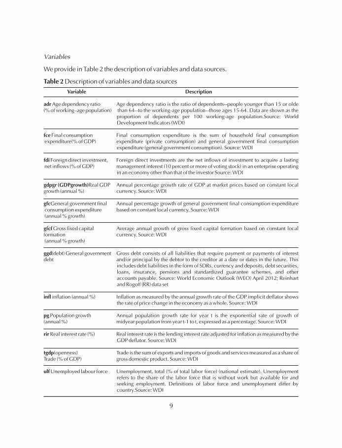
Variables

We provide in Table 2 the description of variables and data sources.

Description of variables and data sourcesTable 2

Variable Description

adr

fce

fdi

gdpgr (GDPgrowth)

gfc

gfcf

ggd

infl

pg

rir

tgdp

ulf

Age dependency ratio Age dependency ratio is the ratio of dependents--people younger than 15 or olde(% of working–age population) than 64--to the working-age population--those ages 15-64. Data are shown as the

proportion of dependents per 100 working-age population.Source: WorldDevelopment Indicators (WDI)

Final consumption Final consumption expenditure is the sum of household final consumptionexpenditure(% of GDP) expenditure (private consumption) and general government final consumption

expenditure (general government consumption). Source: WDI

Foreign direct investment, Foreign direct investments are the net inflows of investment to acquire a lastingnet inflows (% of GDP) management interest (10 percent or more of voting stock) in an enterprise operating

in an economy other than that of the investor Source: WDI

Real GDP Annual percentage growth rate of GDP at market prices based on constant localgrowth (annual %) currency. Source: WDI

General government final Annual percentage growth of general government final consumption expenditureconsumption expenditure based on constant local currency. Source: WDI(annual % growth)

Gross fixed capital Average annual growth of gross fixed capital formation based on constant localformation currency. Source: WDI(annual % growth)

(debt) General government Gross debt consists of all liabilities that require payment or payments of interestdebt and/or principal by the debtor to the creditor at a date or dates in the future. This

includes debt liabilities in the form of SDRs, currency and deposits, debt securities,loans, insurance, pensions and standardized guarantee schemes, and otheraccounts payable. Source: World Economic Outlook (WEO) April 2012; Reinhartand Rogoff (RR) data set

inflation (annual %) Inflation as measured by the annual growth rate of the GDP implicit deflator showsthe rate of price change in the economy as a whole. Source: WDI

Population growth Annual population growth rate for year t is the exponential rate of growth of(annual %) midyear population from year t-1 to t, expressed as a percentage. Source: WDI

Real interest rate (%) Real interest rate is the lending interest rate adjusted for inflation as measured by theGDP deflator. Source: WDI

(openness) Trade is the sum of exports and imports of goods and services measured as a share ofTrade (% of GDP) gross domestic product. Source: WDI

Unemployed labour force Unemployment, total (% of total labor force) (national estimate). Unemploymentrefers to the share of the labor force that is without work but available for andseeking employment. Definitions of labor force and unemployment differ bycountry.Source: WDI

3 THE DEBT – GROWTH RELATIONSHIP

In economic theory, at moderate levels of government debt, following typical Keynesianbehaviour, fiscal policy may induce growth. The classical economic view argues thatgovernment debt (manifesting deficit financing) can induce growth by stimulating aggregatedemand and output in the short run. Moderate levels of debt are found to have a positiveimpact on economic growth through a range of channels: improved monetary policy,strengthened institutions, enhanced private savings, and deepened financial intermediation(Abbas and Christensen 2007). Government debt could be used to smoothen distortionarytaxation over time (Barro 1979). Barro’s model predicts that debt responds to the temporarydeviation in income or government expenditure and hence, in the absence of aggregateuncertainty, debt would be constant and equal to its ‘initial’ level. Expansionary fiscal policiesthat lead to debt accumulation are argued to have a positive effect on both short- and long-term growth (DeLong and Summers 2012). In a theoretical model integrating the governmentbudget constraint and debt financing, Adam and Bevan (2005) find increase in growth duringlow debt levels as they observe interaction effects between deficits and debt stocks, with highdebt stocks exacerbating the adverse consequence of high deficits.

Historically, the theoretical literature argues that growth models amplified withgovernments issuing debt to fund consumption or capital goods tend to exhibit a negativerelationship between government debt and economic growth. Modigliani (1961) argues thatgovernment debt is a burden for posterity, which results in waning flow of income from areduced stock of private capital. It is argued that government debt crowds out capital andleads to a slowdown of output in the long run (Elmendorf and Mankiw 1999).

Both the neoclassical and endogenous growth models inform of the negative effect ofgovernment debt on long-run growth. Government debt could have a substantial adverseeffect on economic outcomes if it affects the productivity of public expenditures (Teles andCesar Mussolini 2014). Analysing the impact of fiscal policy, proxied inter alia by the level ofgovernment debt, in endogenous growth models, Aizenman et al. (2007) find a negativerelationship. While standard growth theory advocates that an increase in government debt(due to a fiscal deficit) leads to slower growth, the neoclassical growth theory suggests atemporary decline in growth along with the transition path to a new steady state. However,the endogenous growth theory suggests a permanent decline in growth as the debt increases(Saint–Paul 1992).

Several studies report a negative non–linear correlation between government debt andeconomic growth in advanced and emerging market economies (Reinhart and Rogoff 2010;Reinhart et al 2012; Kumar and Woo 2010; Cecchetti et al. 2011; Checherita-Westphal andRother 2012). There is growing evidence that government debt is negatively correlated witheconomic growth, and very few studies make a strong case for a causal relationship going

.

10

from debt to growth. Using data on 20 developed countries, Lof and Malinen (2014) estimatepanel vector auto regressions to analyse the relationship between government debt andeconomic growth, and find no evidence for a robust effect of debt on growth, even for higherlevels of debt. However, they observe significant negative correlation due to reverse effect ofgrowth on debt. This study intends to provide a thorough analysis based on a larger data setand further refining with the analyses of the debt–growth nexus in debt regimes.

We embark on a multi–step approach to explore our secular dataset covering the period from1960 to 2009 and thoroughly investigate the nexus between government debt and growth.We employ both the descriptive statistics approach (as relied upon by Reinhart and Rogoff(2010) in their influential paper) and econometric approach to illustrate the nexus betweengovernment debt and economic growth.

3.1.1 Testing the Bivariate Relationship

In our econometric approach to address the topic, we begin by probing the bivariate linearrelationship between debt and growth with the following specification:

We probe the linear relationship with an empirical specification based on the empiricalgrowth literature (e.g. Barro and Sala-i-Martin 2004). We introduce other significantmacroeconomic variables to account for their simultaneity of impact. We are motivated byIslam (1995) in estimating our panel data growth regressions with country-specific fixedeffects and time-specific fixed effects, which allows us to estimate the impact of a change inany one factor on growth a country in the data panel.

— Eqn (3)

Where is country fixed effects; is time fixed effects; is the error term.

3.1.3 The Augmented Solow Growth Regression Model

We extend our econometric specification using a Solow growth model. Following thismodel, our specification assumes that the structural growth for country ‘ ’conforms to a linearrelationship over a period‘t’and is common across the panel of countries.

3.1 Estimation Strategy

GDPgrowth = + ------------- Eqn (2)

Where GDPgrowth is the annual GDP growth and debt is the outstanding grossgovernment debt-to-GDP ratio for country ‘ ’ in year ‘ t’. We estimate Eqn (2) with a pooledpanel and with country fixed effects.

3.1.2 Testing the Linear Relationship

GDP = + debt + (gfcf ,fce ,tgdp ,fce ,fdi ) + + +

j j

j j

j j j j j j j j

t t t

t t

t t–1 t t t t t t t t jt

t jt

a+b e

a+b g j m n e

n e

debt

j

growth GDP

within

µ

j

j t

11

GDP = + + +

GDP = S + debt + + +

GDP = S + debt + debt + + +

growth X

growth

growth

j j

j j

j j 2j

t t t t jt

t s j t t t jt

t s j t t t t jt

b m n e

b g m n e

b g g m n e

Ù

Ù

Ù Ù Ù

——— Eqn (4)

Where is a vector of Solow regressors including ,and It also includes the constants. is country-specific fixed effects; is

time–fixed effects; is the unobservable error term. Given the strong potential forendogeneity of the debt variable, we use the instrumental variable (IV) estimation technique.In our instrumental variables model, we use Solow instruments in their lagged variables. AsEasterly and Rebelo (1993) observe, one of the most likely sources of simultaneity is businesscycle effects and, hence, the tendency of government expenditure is positively correlatedwith the level of GDP per capita. Many studies on growth regressions exploring panel datahave made use of the IV approach to deal with the issue of simultaneity bias Hiebert(2002). With the use of the GMM estimator, we seek to correct for the possibleheteroscedasticity and autocorrelation in the error structure by using the consistent estimator.The two-step GMM provides some efficiency gains over the traditional IV/2–SLS estimatorderived from the use of the optimal weighting matrix (Baum et al. 2013).

3.1.4 Testing for Non-linearity

In the debt–growth dynamics literature, the non-linearity of the impact of debt on economicgrowth has been examined in different specifications. Reinhart and Rogoff (2010) use thecorrelations between debt and growth. On the other hand, Kumar and Woo (2012) and Egert(2015) study the relationship using the growth framework. While many empirical papersidentify non-linearities in the relationship between debt and growth, very few studies make aclear theoretical argument for the presence of such non-linearities (Greiner 2013).

We investigate the non-linearity of the debt–growth relationship (in view of the negativecorrelations at higher levels of debt with growth) by considering a specification that accountsfor the polynomial trend of the debt variable. To introduce the smooth transition around aturning point in debt level, we transform the Eqn (4) to formulate the following specificationby introducing a square term of the debt-to-GDP ratio as an additional regressor:

——— Eqn (5)

3.1.5 Robustness Checks

To ensure that the outliers do not influence the results, we identify the outliers by drawing thescatter plot of the partial correlation between debt and growth obtained with the IV regressionand estimate the models by dropping them. We also employ the robust least squares (RLS)regression method, which is designed to be less sensitive to outliers. We use the M-estimationmethod of RLS. Using the Huber–White sandwich correction, serially correlated residuals are

S gfcf, gfc, tgdp, fce, fdi, infl lagged

GDP, pg, adr. µ í

å

et al.,

j

j t

jt

12

dealt with in the context of the presence of within-country time dependence andheteroscedasticity of unknown form. An alternative approach of using the Newey and Westestimator (which allows for modeling the autocorrelation process in the error term) is alsoemployed. The method of PCSEs (suggested by Beck and Katz)is very robust when there islittle or no correlation between unit effects and explanatory variables. It is argued that itsperformance declines as the correlation strengthens. We use the fixed effects estimator withrobust standard errors that appears to do better in these situations (Kristensen and Wawro2003). In addition, we test for the causality running from debt to growth employing PairwiseDemitrescu–Hurlin Panel Causality Tests. The results shown in Table 3 are significant andindicate causality running in both directions, i.e. from debt to growth and growth to debt.

We provide in Figure 4 a graphical analysis of the correlation between debt and growthin the debt regimes discretely. In the debt regimes: 0-30%, 31-60% and 61-90% debt/GDPlevels, the GDP growth hovers in the positive level and tends to glide into the negative zone inthe debt regime 91-150%. In the debt regime >151% debt/GDP level, the GDP growth runs inthe negative zone demonstrating the negative relationship with debt level.

Table 3 Results of pairwise Demitrescu–Hurlin panel causality tests

We discuss the results of the econometric analysis of the debt–growth relationshipencompassing the econometric specifications for (1) testing the bivariate relationship asmodeled in Eqn. (2); (2) testing the linear relationship as modeled in Eqn. (3); (3) testing theaugmented Solow growth model in Eqn. (4); and (4) testing for non-linearity as modeled inEqn. (5). Table 4 presents the results of the analyses. As observed in other studies as well,simple bivariate panel regression reveals a negative relation between growth andgovernment debt. Though the coefficient is always negative, its size is mostly not substantialin economic terms. The point estimates of the range of econometric specifications suggestthat a 10-percentage-point increase in the debt-to-GDP ratio is associated with a 2–23-basis-point reduction of average growth.

Our results are comparable to the estimates of Kumar and Woo (2010) and Égert Balázs(2015) for advanced and emerging economies over almost four decades. Studying a sampleof 17 OECD countries, Panizza and Presbitero (2014) observe that a 10-percentage-pointincrease in the debt-to-GDP ratio is associated with an 18-basis-point decline in averagegrowth.

Specification Null Hypothesis: W–Stat. ZbarStat. Prob.

1 GDP growth does not homogeneously cause debt 4.6265 6.0140 2.00E-09Debt does not homogeneously cause GDP growth 3.5252 3.0872 0.002

3

13

Figure 4 Government debt and growth in debt regimes

This figure presents the dynamics of government debt and economic growth in debt regimes: 0-30; 31-60; 61-90; 91-150; 151% and above over1960–2009.

14

Table

4D

ebt a

ndG

row

th–

Reg

ress

ion

Res

ults

This

tabl

epr

esen

tsth

ere

sults

ofth

ere

gres

sion

sfo

run

ders

tand

ing

the

effe

ctof

debt

onth

elo

ng–t

erm

grow

thof

coun

trie

s.O

urde

pend

ent

vari

able

isth

eG

DP

grow

th.

Col

umns

(1),

(2)

and

(5)

pres

ent

the

resu

ltsof

the

Pane

lLe

ast

Squa

res(

PLS)

.C

olum

ns(3

) and

(6) p

rese

ntth

ere

sults

ofth

ePa

nelG

ener

aliz

edM

etho

dof

Mom

ents

(PG

MM

)(Cro

ss–s

ectio

nw

eigh

ts(P

CSE

)st

anda

rder

rors

&co

vari

ance

).C

olum

ns(4

),(5

) and

(7) p

rese

ntth

ere

sults

ofR

obus

t Lea

stSq

uare

s.W

ere

port

the

coef

ficie

ntva

lues

mar

ked

with

sign

ifica

nce

leve

lsin

the

first

row

follo

wed

byth

est

anda

rder

rors

(inth

epa

rent

hesi

s)in

the

seco

ndro

w.A

ster

isks

***,

**in

dica

tele

vels

ofsi

gnifi

canc

eat

1%,a

nd5%

resp

ectiv

ely.

Expla

nat

ory

Var

iable

s

Gen

eral

gov

ernm

ent g

ross

debt

(Deb

t)

Deb

t Sq.

GD

PGR

(-1)

Gro

ss fi

xed

capi

tal f

orm

atio

n

Gov

ernm

ent e

xpen

ditu

re

Trad

e O

penn

ess

Fina

l con

sum

ptio

nxp

endi

ture

Fore

ign

dire

ct in

vest

men

t

Infla

tion

Inte

rcep

t

R-s

quar

edO

bs

Mea

n (

Std. D

ev.)

56.1

16 (5

6.46

)

3912

(311

39)

3.85

42 (5

.49)

5.85

72 (4

2.10

)

4.66

68 (1

8.54

)

72.8

92 (5

1.74

)

81.2

41 (1

3.71

)

2.73

57 (4

.62)

1.69

75 (1

.22)

45.1

31 (5

52.4

7

-0.0

14**

*

-0.0

14**

*(0

.109

)

Popu

latio

n gr

owth

0.17

936

07

8.12

8***

(1.2

54)

0.00

3***

(0.0

02)

0.21

8***

(0.0

18)

0.29

326

43

8.14

0***

(1.3

86)

-0.0

03*

(0.0

02)

-0.2

18**

*(0

.029

)

0.29

226

40

2.25

9***

(0.3

41)

-0.0

02**

*(0

.001

)

0.26

1***

(0.0

11)

0.30

6***

(0.0

11)

0.18

9***

(0.0

28)

0.24

9***

(0.0

11)

0.35

026

40

3.73

2***

(0.5

44)

-0.0

13**

*(0

.004

)

0.21

926

21

8.19

7***

(1.5

26)

-0.0

23**

*(0

.005

)

0.30

826

21

-0.0

079*

**(0

.002

5)

0.00

0017

8(0

.000

0166

)0.

0000

466*

*(0

.000

0210

)1.

24E-

05**

(1.0

6E25

)

2.46

8***

(0.3

46)

0.35

545

2621

-0.0

01*

(0.0

001)

-0.0

003*

**(0

.000

1)-0

.000

3**

(0.0

001)

-0.0

0075

**(7

.41e

-05)

-0.0

69**

*(0

.014

)-0

.069

***

(0.0

16)

-0.0

12**

*(0

.004

)-0

.019

***

(0.0

06)

-0.0

63**

*(0

.016

)-0

.011

***

(0.0

04)

0.00

1(0

.005

)0.

001

(0.0

05)

0.00

5***

(0.0

01)

0.00

2(0

.002

)0.

004

(0.0

05)

0.00

5***

(0.0

01)

0.06

1***

(0.0

20)

0.05

9***

(0.0

22)

-0.0

03**

*(0

.011

)-0

.063

***

(0.0

18)

-0.0

53**

(0.0

21)

-0.0

019*

**(0

.011

4)

0.01

3***

(0.0

03)

0.01

3**

(0.0

05)

0.01

5***

(0.0

02)

0.04

0***

(0.0

06)

0.03

3***

(0.0

08)

0.01

7***

(0.0

03)

0.19

8***

(0.0

42)

0.02

92**

*(0

.067

)0.

126*

**(0

.218

)0.

223

(0.0

42)

0.01

5***

(0.0

02)

-0.0

15**

*(0

.004

)0.

181*

**(0

.001

)0.

014*

**(0

.002

)0.

015*

**(0

.004

)0.

181*

**(0

.009

)

15

4 DECOMPOSING THE CAUSE–EFFECT RELATIONSHIP

In this section, we decompose the cause–effect relationship between debt and growth and tryto answer the question: Does high debt lead to low growth or low growth leads to high debt?Our approach here is to study the macroeconomic analyses of the debt–growth relationshipby considering the interdependencies across sectors, markets, and countries, and nationaleconomic issues that are required to be confronted from a global perspective; that is, differentchannels of transmission need to be considered. A useful approach to deal withinterdependent economies is to construct panel vector auto regressions (PVAR ) models.

Our PVAR has almost the same structure as VAR models in the sense that all variables areassumed to be endogenous and interdependent, but we add a cross sectional dimension tothe expression. Let us consider that Y is the stacked version of y = (y' , y' , y' ). Accordingly,our PVAR specification is :

y = A (t) + A (t) Y + u i = 1,...., N t = 1,......, T ........Eqn (1)

4

The model

t it 1t 2t 3t

it oi t t–1 it

The subscripts and denote country and year, respectively. U is a vector of randomdisturbances and, as the notation suggests, A (t) and A depend on the country. A (t) is acountry-specific fixed effect intercept term. Thus, Eqn (1) includes constants, seasonaldummies, and deterministic polynomials in time. The coefficient matrix A and thecovariance matrix of the residuals are assumed as homogeneous. With this assumption, weestimate the pooled estimates of A that can be used to compute the impulse response (IR)functions. The confidence intervals of IR functions are estimated with bootstrap simulations.We impose a recursive structure to identify the shocks that makes the order of the variablespertinent. We also consider the PVAR in reverse recursive order as a robustness check to findout whether the imposed order has a substantial effect on the results.

In order to test the robustness of the model, is performed whichreports the multivariate LM test statistics for residual serial correlation up to the specifiedorder. We perform the wherein the test regression is run byregressing each cross product of the residuals on the cross products of the regressors andtesting the joint significance of the regression. The test is with both options of 'no cross terms'and 'with cross terms'.

To analyse the dynamic association between debt and GDP growth, we compute theimpulse response functions from the estimated PVAR. We estimate the PVAR using the fixedeffects (FE) estimator. Baltagi (2008) suggests first differencing the panel models to eliminatethe fixed effect to the inconsistencies. Since our sample size is adequately large, we go aheadwith the FE estimator. However, as a robustness check, we find the GMM estimates of thefirst–differenced model with similar results.

i t

Autocorrelation LM Test

White Heteroskedasticity Test,

it

oi i oi

i

i

16

We use the same data sets as detailed in Section 2 and consider all the five debt regimes(0-30%, 31-60%, 61-90%, 91-150%, and >151%) as well as the full sample (including alldebt regimes) for PVAR analysis.

Table 5 Sample description for debt regimes for PVAR analysis

We present the impulse–response functions derived from the estimated PVAR in Figure 5. Thefigure shows the effect of debt on GDP growth for a period of ten years after a positive shock.In the debt regime 0–30, the impulse response function of GDP growth to one standarddeviation shock to debt reaches the peak level of 1.17% in the fourth year and graduallyrecedes. When we extend the period to 30 years, we notice the response touching almostzero level (0.04% in the 11 year to 0.0006% in the 30 year).

In the case of debt regime 31–60, the impulse response function of GDP growth to onestandard deviation shock to debt reaches the peak of 0.86% in the third year and graduallydecreases to 0.03% in the tenth year. When the period is extended to 30 years, the responsecontinues to be in the range of 0.03% to 0.07% but never merges into zero.

Debt regime 61–90 has an interesting behaviour. The impulse response of GDP growthto one standard deviation shock to debt moves from negative zone to positive zone (-0.5% inthe second year, -0.04% in the tenth year, 0.002% in the 16 year and 0.03% in the 30 year).In the debt regime 91–150, the impulse response of GDP growth moves in the range of -0.32% in 2 year to 0.13% in the 10 year. When the period is extended to 30 years, theimpulse response of GDP growth reaches 0.02% in the 30 year.

Debt regime 151 and above experiences a distinct behaviour. The impulse response ofGDP growth moves in the range of 1.03% in the first year to 0.04% in the tenth year. In theextended period (up to 30 years), the impulse response of GDP growth reaches almost zero(0.000038%). We also analyse the impulse response of GDP growth in the full sample(including all the debt regimes). The impulse response of GDP growth moves in the range of1.26% in the second year to -0.87% in the 10th year. The above results suggest that theimpulse response function for the effect of debt on GDP growth is dependent on the debtregimes and there is no uniformity of effect across the debt regimes. We notice a long–termeffect of debt on growth.

Period DR 0-30% DR 31-60% DR 61-90% DR 91 & above DR 151 & above1960-2009 29 56 18 14 5

Total122

Results

th th

th th

nd th

th

3

4

Kumar and Woo (2010) report that on average, a 10-percentage-point increase in the initial debt-to-GDP ratio isassociated with a slowdown in annual real per capita GDP growth of around 0.2 percentage points per year. ÉgertBalázs (2015) find that a 10-percentage-point increase in the government debt ratio is associated with a 0.1–0.2-percentage-point lower economic growth.

These PVARs seek to capture the dynamic interdependencies using a minimal set of restrictions. Shockidentification then transforms these reduced form models into structural ones, allowing for typical exercises such asimpulse response analyses or policy counterfactuals. PVARs are mostly suited to capture both static and dynamicinterdependencies-while treating the links across units in an unrestricted fashion. They easily incorporate timevariations in the coefficients and account for cross-sectional dynamic heterogeneities. They are a powerful tool toaddress interesting policy questions related, for example, to the transmission of shocks across borders.

17

5 It uses the inverse of the Cholesky factor of the residual covariance matrix to orthogonalise the impulses. This optionimposes an ordering of the variables in the VAR and attributes all of the effect of any common component to thevariable that comes first in the VAR system.

18

Figure 5 Impulse response function of GDP growth to debt innovation

This figure illustrates the impulse response functions of GDP growth to Cholesky one standard deviation debtinnovation computed from estimated PVAR (Eqn. 1) in all the five debt regimes (0-30; 31-60; 61-90; 91-150; and 151and above) and for the full sample covering all debt regimes. The dashed lines enclose intervals of plus or minus twostandard errors.

5

Figure 6 Impulse response function of debt to GDP growth

This figure illustrates the impulse response functions of debt to Cholesky one standard deviation growth innovationcomputed from estimated PVAR (Eqn. 1) in all the five debt regimes (0-30; 31-60; 61-90; 91-150; and 151 and above)and for the full sample covering all debt regimes. The dashed lines enclose intervals of plus or minus two standarderrors.

19

From Figures 5 and 6, it appears that the negative relationship between debt and GDPgrowth is the consequence of the negative effect of GDP growth on debt, rather than thenegative effect of debt on GDP growth. Thus, there is evidence of GDP growth having asignificant negative effect on debt.

Accumulated response of GDP growth to debt innovationFigure 7

This figure illustrates the accumulated impulse response functions of GDP growth to Cholesky One standarddeviation debt innovation computed from estimated PVAR (Eqn. 1) in all the five debt regimes (0-30; 31-60; 61-90;91-150; and 151 and above) and for the full sample covering all debt regimes. The dashed lines enclose intervals ofplus or minus two standard errors.

20

We now present the results based on the accumulated responses. Figure 7 provides thecumulative impulse response functions estimated from PVAR for all the debt regimes and fullsample. By accumulating the impact over time, these plots indicate the accumulated impulseresponse functions of GDP growth to Cholesky one standard deviation debt innovation. Theresults are interesting. For the 0–30 per cent debt regime, we find that a shock to debt has asignificant positive effect on GDP growth. The accumulated response of GDP growth for theimpulse from debt appears to be positive in the long run as we notice an increasingcumulative response for one standard deviation shock to debt (1.81% in the 4th year, 3% inthe 7th year and 3.19% in the 10th year). We verify the relationship for a 30-year period aswell, and notice the response as high as 3.81%. Variance decomposition of GDP growth forthe 10-year period in the debt regime 0-30 shows that up to 10% of the variation in GDPgrowth could be dependent on variation in debt.

We find that a shock to debt has significant positive effect on GDP growth in the debtregime 31-60 as well. The cumulative response of GDP growth (for one standard deviationshock to debt) rises from 0.75 % in the 3rd year to a high of 2.17 % in the 10th year. When weextend the period up to 30 years, the response continues to be upward (2.31% in the 30thyear). The results suggest that countries in the debt regime 31–60 experience a phenomenonwherein debt has a long-term positive effect on GDP growth. Variance decomposition ofGDP growth for the 10–year period in the debt regime 31-60 shows that up to 4.39% of thevariation in GDP growth could be explained by variation in debt. We notice an interestingbehaviour of GDP growth towards debt shock in the case of debt regime 61–90. Thecumulative response of GDP growth, for one standard deviation debt innovation at 34.40,hovers around a petite negative range of -0.04% to -0.14 % in a period of ten years. When weextend the period to 30 years, the cumulative response hovers around the same tiny range of -0.04% -0.15%. These results suggest that countries in this debt regime 61–90 fail to generatesignificant growth response for debt shocks. Variance decomposition of GDP growth for the10–year period in the debt regime 61–90 suggests that up to 2.16% of variation in GDPgrowth could be due to variation in debt. Debt regime 91–150 displays an interestingbehaviour of GDP growth to debt shock. The accumulated response of GDP growth to debtshock continues to be negative up to the initial three years and traverses slightly into thepositive zone during the 4th and 5th years and again moves back into the negative zone fromsixth to eighth year. When we extend the analysis for a longer period (up to 30 years), wenotice the response of GDP growth (for one standard deviation shock to debt) to be swingingin the range of -1.6% to 1.62%. The results show that GDP growth has no straightforwardassociation with debt during this debt regime. It is affected largely by other determiningmacroeconomic factors such as inflation, trade openness, gross capital formation, andforeign direct investment. Variance decomposition of GDP growth for the 10-year period inthe debt regime 91–150 suggests that up to 29.41% of variation in GDP growth could be dueto variation in debt.

In the case of debt regime 151 and above, the cumulative response of GDP growthremains negative for the first four years and then turns gradually into a small positive territory.During the 10 year period of analysis, we notice the cumulative response of GDP growth (for

21

one standard deviation shock to debt) to hover in the range of -0.17% to 0.49%. When weextend the period to 30 years, the GDP growth response to reaches a high of 0.52%. Variancedecomposition of GDP growth for the 10–year period in the debt regime 91-150 suggests thatup to 19.82% of the variation in GDP growth could be due to variation in debt. Theaccumulated response of GDP growth to debt shock swings in the range of -3.53% in the 6thyear to 1.45% in the 9th year for the full sample including all debt regimes. Variancedecomposition of GDP growth for the 10–year period for the full sample suggests that up to40.04% of variation in GDP growth could be due to variation in debt.

This analysis has thus provided useful insights about debt dynamics in the debt regimegroupings of 0-30%, 31-60%, 61-90%, 91-150%, and >151%, comparable to Reinhart &Rogoff's groupings based on average debt/GDP levels. The mean GDP growth rates are DR 0-30: 5.06%; DR 31-60: 3.79%; DR 31-60: 2.71%; DR 91-150: 1.86%; and DR 151 and above-1.08%. Countries in DR 0-30 experience a rising trend of debt. It suggests that in thesecountries with debt (mean 27.15, median 27.79) has a positive effect on economic growth.Countries in DR 31-60 experience a flat trend of debt (mean 58.29, median 45), suggestingthat, countries reach their optimum gains for boosting their economic growth at this level ofdebt. Countries in DR 61-90 with debt (mean 80.08, median 82.87) on the other handexperience a gentle declining trend. It shows that countries tend to experience noincremental gains from debt and perhaps approaching their debt thresholds. Countries in DR91-150 with debt (mean115.50, median116.51) show a downward trend suggesting that mostof them might have hit their debt thresholds. Finally, countries in DR 151 & above with debt(mean 176.75, median 160.99), experience a sweeping downward growth indicating thenegative effects of excess debt.

Our results derived from PVAR estimations clearly show the evidence of the effect ofdebt on economic growth. Therefore, our results do not concur with the conclusion of Lof andMalinen (2014) that there is no evidence of for a robust effect of debt on growth, even forhigher levels of debt in their analysis of 20 developed countries. Our results also indicate thatthe effect is not uniform for all countries, but mostly depends on the debt regimes and otherimportant macroeconomic variables such as inflation, trade openness, general governmentfinal consumption expenditure and foreign direct investment.

This study has presented a thorough data-rich analysis of the dynamics of government debtand economic growth for a longer period, 1960–2009, as it spans different debt regimes andinvolves a worldwide sample of countries that is more representative. The sources on whichthe study draws are more authentic and well accepted. We do not claim that the results areinfallible but do state that they are based on widely accepted econometric tools andtechniques, besides based on sound economic logic. One of the contributions of this study isthat it is the first of its kind in providing a meticulous analysis of the debt–growth nexussupported with a VAR analysis. The study provides an original analysis of debt and growthbeyond the popular discourse, surrounding mostly advanced countries. This study observes anegative relationship between government debt and growth. The point estimates of the range

5 CONCLUSION

22

of econometric specifications suggest a 10-percentage-point-increase in the debt-to-GDPratio, which is associated with a 2–23-basis-point reduction in average growth. Our resultsestablish the non-linear relationship between debt and growth. By analysing thedecomposition of the cause–effect relationship between debt and growth, the study answersthe question: Does high debt lead to low growth, or does low growth lead to high debt? ThePVAR approach was used to study the macroeconomic analyses of the debt–growthrelationship by considering the interdependences existing across sectors, markets, andcountries, and national economic issues. The results derived from the impulse responsefunctions and variance decomposition suggest the evidence of a long-term effect of debt oneconomic growth. The results indicate that the effect is not uniform for all countries butdepends mostly on the debt regimes and other important macroeconomic variables such asinflation, trade openness, general government final consumption expenditure, and foreigndirect investment.

23

REFERENCES

Abbas S M Ali, and Christensen, Jakob. (2007). The Role of Domestic Debt Markets inEconomic Growth: An Empirical Investigation for Low–Income Countries and EmergingMarkets. IMF Working Paper No. 07/127

Adam C S and Bevan D L. (2005). Fiscal deficits and growth in developing countries. Journalof Public Economics 4: 571–597.

Aizenman J, Kletzer K and Pinto B. (2007). Economic growth with constraints on tax revenuesand public debt: implications for fiscal policy and cross-country differences. NBERWorking Paper 12750

Baum A, Checherita C W and Rother P. (2013). Debt and growth: New evidence for theeuroarea. Journal of International Money and Finance 32: 809–821

Barro RJ. (1979). On the determination of the public debt. The Journal of Political Economy87 (5): 940–971.

Barro R and X Sala-i-Martin. (2004).Economic growth, second edition, MIT Press ChecheritaCristina-Westphal and Rother Philipp. (2012). The impact of high government debt oneconomic growth and its channels: An empirical investigation for the euro area.

European Economic Review 56: 1392–1405 Cecchetti Stephen, Madhusudan Mohanty andFabrizio Zampolli. (2011). The real effects of debt. BIS Working Papers No. 352, Bank forInternational Settlements.

EgertBalazs. (2015). Public debt, economic growth and nonlinear effects: Mythor reality?Journal of Macroeconomics 43: 226–238

Elmendorf Douglas W and Gregory MankiwN. (1999). Government Debt. In (J. B. Taylor& M. Woodford (ed.)) Handbook of Macroeconomics 1(3): 1615-1669.

Easterly W and Rebelo S. (1993). Fiscal Policy and Economic Growth: An EmpiricalInvestigation. Journal of Monetary Economics 32(3): 417-58.

Greiner Alfred. (2013). Debt and Growth: Is there a non-monotonic relation? EconomicsBulletin 33 (1): 340-347

Herndon T, Ash M, Pollin R. (2014). Does high public debt consistently stifle economicgrowth? A critique of Reinhart and Rogoff. Cambridge Journal of Economics 38(2):257–279.

Islam N. (1995). Growth empirics: a panel data approach.Quarterly Journal of Economics110: 1127–70.

KristensenIda Pagter and Wawro Gregory. (2003). Lagging the Dog? The Robustness of PanelCorrected Standard Errors in the Presence of Serial Correlation and Observation SpecificEffects. Working Paper No. 54. Washington University in St. Louis. Extracted fromhttp://polmeth.wustl.edu/mediaDetail.php?docId=54

24

Krugman, Paul (2010). “Reinhart and Rogoff Are Confusing Me.” New York Times, 11August.

Kumar Manmohan S and Jaejoon Woo. (2010). "Public Debt and Growth", IMF WorkingPapers, No. 10/174, International Monetary Fund

LofMatthijs and Malinen Tuomas. (2014). Does sovereign debt weaken economic growth? APanel VAR analysis. Economic Letters 122(3): 403–407

Modigliani F. (1961). Long-Run Implications of Alternative Fiscal Policies and the Burden ofthe National Debt. Economic Journal 71 (284): 730-755.

Panizza Ugo and PresbiteroAndrea F. (2014). Public debt and economic growth: Is there acausal effect? Journal of Macroeconomics 41: 21–41

Reinhart Carmen M and Kenneth S Rogoff. (2010a). “Debt and Growth Revisited",VoxEU.org, 11August.

Reinhart Carmen M and Kenneth Rogoff S. (2010b). Growth in a Time of Debt. AmericanEconomic Review: Papers and Proceedings 100(2):573-578.

Reinhart Carmen M, Vincent R Reinhart and Kenneth S Rogoff (2012).Public debtoverhangs:Advancedeconomyepisodes since 1800.Journal of Economic Perspectives26(3): 6986.

Saint-Paul (1992). Fiscal Policy in an Endogenous Growth Model. Quarterly Journal ofEconomics 107(4): 1243–59.

Teles VK and Cesar MussoliniC. (2014). Public debt and the limits of fiscal policy to increaseeconomic growth. European Economic Review 66: 1–15.

25

APPENDICES

Annexure 1: Countries covered in Debt Regime groupings

1 DR 0-30 (21) Azerbaijan, Bahrain, Botswana, Chile, China,Colombia, Congo, Rep., Czech Republic, Estonia, Finland,Germany, Guatemala, Kazakhstan, Latvia, Namibia, Norway,Oman, Paraguay, Romania, Slovenia, and Thailand.

2 DR 31-60 (31) Argentina, Austria, Brazil, Canada, Denmark,Dominican Republic, Ecuador, El Salvador, France, Ghana,Iceland, India, Indonesia, Japan, Kenya, Malaysia, Mexico,Netherlands, New Zealand, Peru, Philippines, Portugal, SouthAfrica, Spain, Sweden, Tunisia, Turkey, United Kingdom, UnitedStates, Uruguay, and Venezuela, RB.

3 DR 61-90 (22) Algeria, Bolivia, Costa Rica, Cote d'Ivoire, Egypt,Arab Rep., Egypt, Arab Rep., Greece, Ireland, Panama, andSingapore.

4 DR 91-150 (8) Belgium, Burundi, Central African Republic,Honduras, Italy, Jamaica, Jordan, Kyrgyz Republic, Madagascar,Nigeria, Seychelles, Sri Lanka, and Tajikistan.

5 DR 151 and above (5) Congo, Dem. Rep., Cyprus, Malta,Nicaragua, and Zambia

26

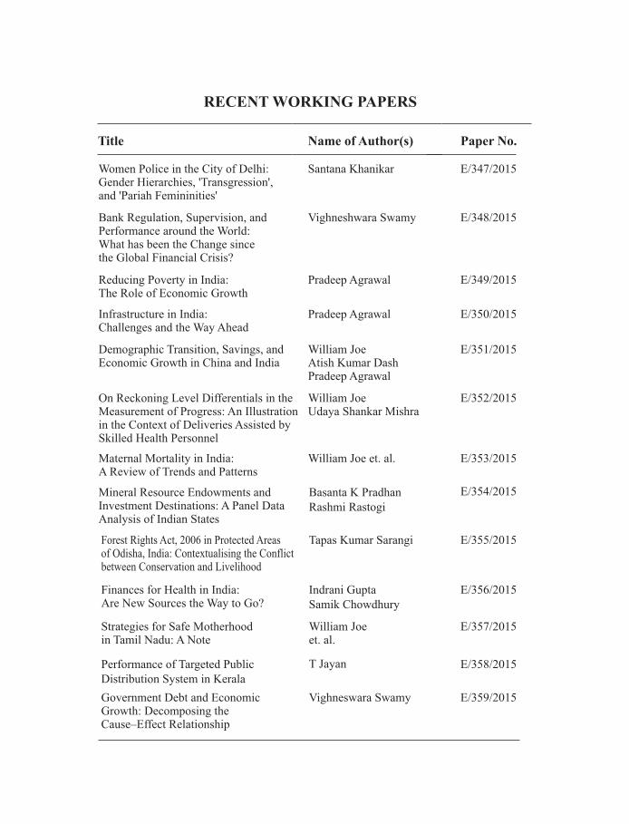
RECENT WORKING PAPERS

Title Name of Author(s) Paper No.

Women Police in the City of Delhi:Gender Hierarchies, 'Transgression',and 'Pariah Femininities'

Bank Regulation, Supervision, andPerformance around the World:What has been the Change sincethe Global Financial Crisis?

Reducing Poverty in India:The Role of Economic Growth

Santana Khanikar

Vighneshwara Swamy

Pradeep Agrawal

E/347/2015

E/348/2015

E/349/2015

Infrastructure in India:Challenges and the Way Ahead

Pradeep Agrawal E/350/2015

William JoeAtish Kumar DashPradeep Agrawal

Demographic Transition, Savings, andEconomic Growth in China and India

E/351/2015

William JoeUdaya Shankar Mishra

On Reckoning Level Differentials in theMeasurement of Progress: An Illustrationin the Context of Deliveries Assisted bySkilled Health Personnel

E/352/2015

William Joe et. al.Maternal Mortality in India:A Review of Trends and Patterns

E/353/2015

Basanta K Pradhan

Rashmi Rastogi

Mineral Resource Endowments andInvestment Destinations: A Panel DataAnalysis of Indian States

E/354/2015

Tapas Kumar SarangiForest Rights Act, 2006 in Protected Areasof Odisha, India: Contextualising the Conflictbetween Conservation and Livelihood

E/355/2015

E/356/2015Indrani Gupta

Samik Chowdhury

Finances for Health in India:Are New Sources the Way to Go?

William Joeet. al.

Strategies for Safe Motherhoodin Tamil Nadu: A Note

E/357/2015

Performance of Targeted Public

Distribution System in Kerala

T Jayan E/358/2015

Government Debt and EconomicGrowth: Decomposing theCause–Effect Relationship

Vighneswara Swamy E/359/2015

lR;eso ijeks /eZ%

Institute of Economic Growth

University Enclave, University of Delhi

Delhi 110007, India

Tel: 27667101/288/424; Fax : 27667410

Website : www.iegindia.org