Gopher Disturbance and Plant Community Dynamics In Montane Meadows

Madelon Case

Department of Ecology and Evolutionary Biology Princeton University

Simon Levin April 30, 2012

 

Acknowledgments

I am grateful to have had all the support I needed to carry out this project. I owe thanks to many people who helped make it happen:

To the Colvin family and the Princeton Environmental Institute, who funded my summer field research with the Becky Colvin Memorial Award.

To Simon Levin, my advisor, who was a steadfast source of insightful questions, advice, and feedback; and to Charlie Halpern, my mentor from the University of Washington, who was exceptionally generous with his time, from spending weeks of his summer helping me with field work at Bunchgrass Ridge, to making himself available whenever I wanted to talk about data analysis and writing. I have learned a tremendous amount from both of them.

To Sarah Koe, the best field assistant I could have asked for.

To the staff at the H.J. Andrews Experimental Forest and the McKenzie River Ranger District who helped make my field research a success.

To the members of the Levin lab who helped me with my analyses: Carla Staver, who introduced me to using R; and Malin Pinsky, who answered my many questions about mixed models.

To all of the Writing Center Fellows and fellow EEB seniors who read and

commented on various portions of my draft in writing workshops. To Emily Rutherford, Rajiv Ayyangar, Kati Henderson, and my parents, Steve and Sarah Case, who also read and responded to drafts. Note

This thesis grew out of research conducted for my Spring Junior Paper. My focus and research plan changed significantly since then, but where appropriate I cite ideas that I first introduced in the JP.

 

This thesis is dedicated to my parents, who have been there whenever I needed encouragement and who taught me to love science and nature in the first place. To my mother especially, who continues to inspire me with her own recovery from disturbance.

 

Table of Contents

List of Figures and Tables …………………………...…………………… 1 Abstract. ………………………………………………………………….. 2 1. Introduction …………………………………………………………..... 3 2. Field Research Methods ……………………………………………….. 14 3. Field Results…………………………………………………………..... 26 4. Simulation Model of Three-Way Plant Interactions………………….... 35 5. Discussion…………………………………………………………….... 43 Appendices A: Brief Overview of Mixed Effects Models……………………… 60 B: Correlogram Plots……………………………………………..... 62 C: Simulation Model Code……………………………………….... 66 Bibliography………………………………………………………………. 69 Honor Pledge ……………………………………………………………... 74

1

List of Figures and Tables Chapter 1 Figure 1.1. Photo of gopher mounds > 1 year old at Bunchgrass Ridge, Oregon. …............ 5 Figure 1.2. Photo of gopher castings soon after snow melt at Bunchgrass Ridge, Oregon. .. 5

Chapter 2 Figure 2.1. Plot layout. ……………………………………………………………............... 17 Figure 2.2. Aerial photo of Bunchgrass Ridge with sampling locations marked. ………..... 18 Figure 2.3. Photo of fresh mound adjacent to old mound. …………………………………. 19 Figure 2.4. Photo of old mound. …………………………………………………………… 20 Figure 2.5. Photo of gopher castings early in the summer. ………………………………… 21

Chapter 3 Table 3.1.Disturbance conditions across plots. …………………………………………….. 26 Table 3.2. Frequency and cover of plant species, summarized by growth form………….... 27 Figure 3.1. Relationship between total cover of disturbance and total cover of plants…….. 28 Figure 3.2. Relationships between total cover of disturbance and (a) total cover of

graminoids and (b) ratio of forb/graminoid cover…………………………………………..

29 Figure 3.3. Relationships between total cover of disturbance and (a) total cover of forbs,

and (b) total cover of forbs with Phlox excluded……………………………………………

30 Figure 3.4. Relationship between total cover of disturbance and transect-level species

richness………………………………………………………………………………………

31 Figure 3.5. Relationship between total cover of disturbance and heterogeneity index.......... 32 Figure 3.6. Relationship between total cover of disturbance and evenness index………...... 32 Table 3.3. Results of mixed-effects models analyzing cover of old mound and cover of

casting as additive fixed effects……………………………………………………………..

33 Table 3.4. Estimated slopes by plot for models with “intercept + slope” random-effects

structure………………………………………………………………………………………

34

Chapter 4 Table 4.1. Reproduction and competition parameters for Species A and B………………… 39 Table 4.2. Reproduction and competition parameters for Phlox……………………………. 40 Figure 4.1. Cover of Species A and B, averaged over 10 simulation trials, for a range of

gopher disturbance in a system where Phlox is absent………………………………………

41 Figure 4.2. Cover of Species A, B and Phlox, averaged over 10 simulation trials, for a

range of gopher disturbance in a system where all three species are present………………..

41

Appendix B Figures B.1-6. Correlogram plots. ………………………………………………………….. 62

   

2

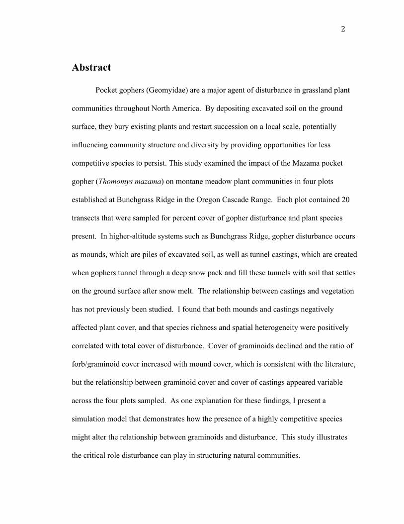
 Abstract

Pocket gophers (Geomyidae) are a major agent of disturbance in grassland plant

communities throughout North America. By depositing excavated soil on the ground

surface, they bury existing plants and restart succession on a local scale, potentially

influencing community structure and diversity by providing opportunities for less

competitive species to persist. This study examined the impact of the Mazama pocket

gopher (Thomomys mazama) on montane meadow plant communities in four plots

established at Bunchgrass Ridge in the Oregon Cascade Range. Each plot contained 20

transects that were sampled for percent cover of gopher disturbance and plant species

present. In higher-altitude systems such as Bunchgrass Ridge, gopher disturbance occurs

as mounds, which are piles of excavated soil, as well as tunnel castings, which are created

when gophers tunnel through a deep snow pack and fill these tunnels with soil that settles

on the ground surface after snow melt. The relationship between castings and vegetation

has not previously been studied. I found that both mounds and castings negatively

affected plant cover, and that species richness and spatial heterogeneity were positively

correlated with total cover of disturbance. Cover of graminoids declined and the ratio of

forb/graminoid cover increased with mound cover, which is consistent with the literature,

but the relationship between graminoid cover and cover of castings appeared variable

across the four plots sampled. As one explanation for these findings, I present a

simulation model that demonstrates how the presence of a highly competitive species

might alter the relationship between graminoids and disturbance. This study illustrates

the critical role disturbance can play in structuring natural communities.

3

Chapter 1

Introduction

Ecologists have long recognized the importance of disturbance in shaping

biological communities. Although equilibrium theories once dominated ecological

discourse, presuming that communities of organisms were stable through time and

existed in a constant environment, it has become apparent that “the normal state of

communities and ecosystems is to be recovering from the last disturbance” (Reice 1994).

A disturbance is a punctuated disruptive event that restarts succession, the process of

change in community structure and composition over time, by killing or damaging

individuals and creating openings for new individuals to establish (Sousa 1984).

Disturbances can vary widely in size and intensity, from a fire that consumes an entire

forest, to the fall of a single tree that opens a gap in the canopy.

We typically think of disturbance in terms of abiotic processes – fire, wind, or

water – that disrupt ecological communities (Sousa 1984). Yet in some systems, the

organisms themselves can be powerful agents of natural disturbance. Gophers are one

such example. Physical disturbances caused by gopher activity often comprise one of the

most frequent and widespread forms of disturbance in grassland plant communities

(Reichman 2007).

The pocket gopher is “a classic example of an ecosystem engineer” (Case 2011,

Reichman & Seabloom 2002), an organism that modifies its physical environment in a

substantial way on a scale that differs from direct biotic interactions such as herbivory

(Hastings et al. 2007). Pocket gophers (Geomyidae) are a family of fossorial rodents that

4

inhabit grassland environments throughout North America. They live almost entirely

underground in complex networks of burrows. This subterranean lifestyle requires that

gophers move a great deal of soil; one estimate puts the average rate of soil excavation by

Geomyidae at 18 m3 ha-1 year-1 (Smallwood & Morrison 1999). Gopher activity can have

profound effects on the abiotic environment of grasslands (Case 2011), creating

heterogeneity in ground-surface topography (Inouye et al. 1987), soil texture (Sherrod &

Seastedt 2001), soil moisture (Kyle et al. 2008), light availability (Inouye et al. 1987),

and nutrient availability (Tilman 1983; Inouye et al. 1987; Sherrod & Seastedt 2001).

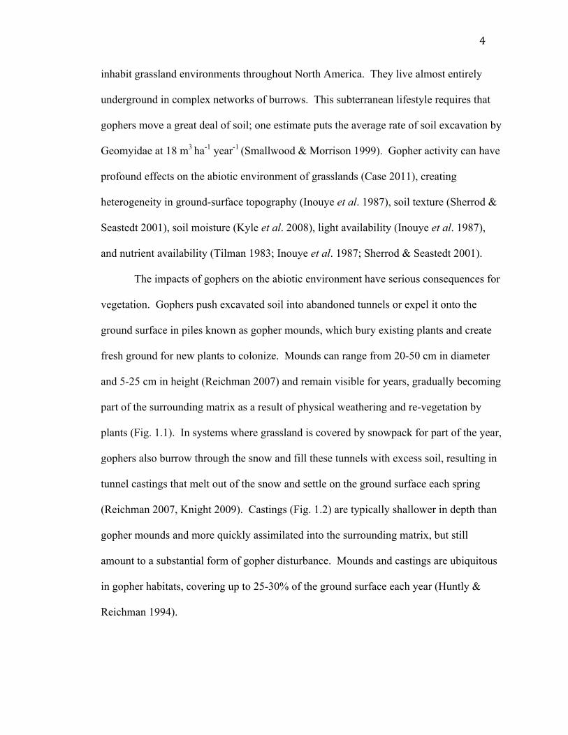
The impacts of gophers on the abiotic environment have serious consequences for

vegetation. Gophers push excavated soil into abandoned tunnels or expel it onto the

ground surface in piles known as gopher mounds, which bury existing plants and create

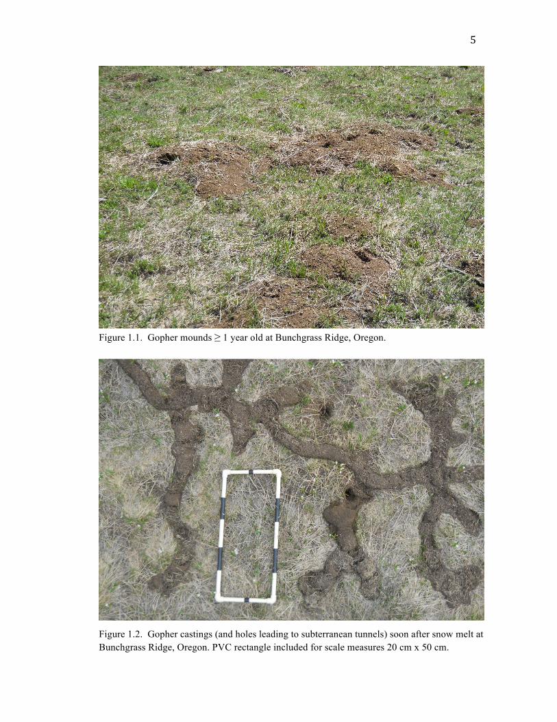
fresh ground for new plants to colonize. Mounds can range from 20-50 cm in diameter

and 5-25 cm in height (Reichman 2007) and remain visible for years, gradually becoming

part of the surrounding matrix as a result of physical weathering and re-vegetation by

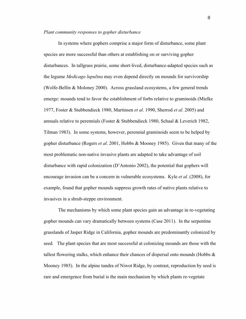
plants (Fig. 1.1). In systems where grassland is covered by snowpack for part of the year,

gophers also burrow through the snow and fill these tunnels with excess soil, resulting in

tunnel castings that melt out of the snow and settle on the ground surface each spring

(Reichman 2007, Knight 2009). Castings (Fig. 1.2) are typically shallower in depth than

gopher mounds and more quickly assimilated into the surrounding matrix, but still

amount to a substantial form of gopher disturbance. Mounds and castings are ubiquitous

in gopher habitats, covering up to 25-30% of the ground surface each year (Huntly &

Reichman 1994).

5

Figure 1.1. Gopher mounds ≥ 1 year old at Bunchgrass Ridge, Oregon.

Figure 1.2. Gopher castings (and holes leading to subterranean tunnels) soon after snow melt at Bunchgrass Ridge, Oregon. PVC rectangle included for scale measures 20 cm x 50 cm.

6

Through studying the ways in which gopher disturbance affects plant community

structure and diversity, we can better understand the powerful role disturbance plays in

shaping ecosystems. In this chapter I will first review the relevant ecological theories

and hypotheses regarding how communities respond to disturbance, then consider how

these phenomena play out in communities affected by gophers, and lastly present the

questions and objectives driving my own study of gopher disturbance and plant

communities in montane meadows of Oregon’s Cascade Range.

Theories of response to disturbance

While the word “disturbance” connotes destruction and damage – and indeed, for

an individual organism that dies in a disturbance event, such negative connotations hold

true – the effects of disturbance at the population and community level can be more

complex. For some species, disturbance represents opportunity. A disturbance event

creates a patch of newly available resources such as space, light, or nutrients. Organisms

that establish quickly after a disturbance – whether by surviving the disturbance and re-

growing, or by colonizing from adjacent or distant patches – can capitalize on the open

niche space and reduced competition (Reice 1994). There are typically trade-offs,

however, between colonization ability and competitive ability. Species adapted to rapid

establishment after disturbance are often less capable of persisting once more competitive

species move in (MacArthur & Wilson 1967, Platt 1975, Connell & Slatyer 1977, Grime

1979).

Higher-level community patterns may emerge from this interplay between

disturbance, competition, and species composition. A fascinating question for ecologists,

7

and a question that has driven much of the research on gopher disturbance, has been

whether disturbance actually facilitates species coexistence and thus maintains diversity.

The Intermediate Disturbance Hypothesis (IDH), a classic non-equilibrium theory of

biological community structure – first proposed by Grime (1973) and further described

by Horn (1977) and Connell (1978) – predicts that maximum species diversity is

maintained at intermediate frequencies and intensities of disturbance. The IDH

postulates that while pioneer species dominate immediately after disturbance, and the

more competitive late-successional species eventually take over, both types of organisms

can coexist at intermediate levels or frequencies of disturbance.

Although the IDH predicts a unimodal, peaked relationship between diversity and

disturbance, empirical studies of disturbance have found that peaked, increasing,

decreasing, and nonsignificant diversity-disturbance relationships are all common

patterns (Mackey & Currie 2001). This may be an outcome of the broad definitions of

terms such as “disturbance” and “diversity,” as well as the question of whether a

sufficient range of disturbance frequency or intensity has been sampled to see a peak at

“intermediate” levels (Sousa 1984). Diversity consists of both species richness (the

number of species) and evenness (the equitability of abundance among species)

(Magurran 2004), and disturbance can have dramatically different effects on these two

parameters within the same system (Reice 1994). Still, the IDH provides a useful

conceptual framework for understanding how disturbance can interact with competitive

hierarchies and facilitate species coexistence, and why disturbance can be considered

important for diversity.

8

Plant community responses to gopher disturbance

In systems where gophers comprise a major form of disturbance, some plant

species are more successful than others at establishing on or surviving gopher

disturbances. In tallgrass prairie, some short-lived, disturbance-adapted species such as

the legume Medicago lupulina may even depend directly on mounds for survivorship

(Wolfe-Bellin & Moloney 2000). Across grassland ecosystems, a few general trends

emerge: mounds tend to favor the establishment of forbs relative to graminoids (Mielke

1977, Foster & Stubbendieck 1980, Martinsen et al. 1990, Sherrod et al. 2005) and

annuals relative to perennials (Foster & Stubbendieck 1980, Schaal & Leverich 1982,

Tilman 1983). In some systems, however, perennial graminoids seem to be helped by

gopher disturbance (Rogers et al. 2001, Hobbs & Mooney 1985). Given that many of the

most problematic non-native invasive plants are adapted to take advantage of soil

disturbance with rapid colonization (D’Antonio 2002), the potential that gophers will

encourage invasion can be a concern in vulnerable ecosystems. Kyle et al. (2008), for

example, found that gopher mounds suppress growth rates of native plants relative to

invasives in a shrub-steppe environment.

The mechanisms by which some plant species gain an advantage in re-vegetating

gopher mounds can vary dramatically between systems (Case 2011). In the serpentine

grasslands of Jasper Ridge in California, gopher mounds are predominantly colonized by

seed. The plant species that are most successful at colonizing mounds are those with the

tallest flowering stalks, which enhance their chances of dispersal onto mounds (Hobbs &

Mooney 1985). In the alpine tundra of Niwot Ridge, by contrast, reproduction by seed is

rare and emergence from burial is the main mechanism by which plants re-vegetate

9

mounds. The traits that confer an advantage in responding to disturbance, therefore, are

quite different there compared to Jasper Ridge; Sherrod et al. (2005) hypothesize that

forbs gain an advantage over graminoids on mounds at Niwot Ridge thanks to greater

belowground carbon stores, which aid in recovery from burial. Comparisons such as

these highlight the importance of studying gopher impacts in a variety of systems.

Support for the Intermediate Disturbance Hypothesis among studies of gopher

disturbance and diversity has been mixed. In a shortgrass prairie community, Martinsen

et al. (1990) found both consistencies and inconsistencies with the IDH. As expected,

species diversity was greatest for plots characterized by disturbances of intermediate age

(supporting the “frequency” dimension of the IDH), but diversity did not differ in plots

with intermediate versus high levels of disturbance. Alternatively, in an abandoned

agricultural field at Cedar Creek in Minnesota, Tilman (1983) found an increase in

richness with level of gopher disturbance in plots. By contrast, Jones et al. (2008) found

that richness increased with age of mounds and peaked in undisturbed vegetation in a

high-altitude meadow in the Pacific Northwest. This would suggest a model of gradual

accumulation of species over time without the inevitable decline in richness predicted by

the IDH. However, this pattern may still be compatible with the IDH if we consider that

even apparently “undisturbed” meadow is still “recovering from the last disturbance”

(Reice 1994) and not in equilibrium. Perhaps species richness would eventually decline

in the absence of further gopher disturbance.

Spatially explicit simulation models, a valuable tool for looking at how fine-scale

processes scale up to emergent patterns, have also been used to investigate the

consequences of various aspects of gopher disturbance patterns for the composition and

10

diversity of plant communities. Such models allow researchers to ask questions that

would be difficult to pursue experimentally (such as how changing the amount of overall

gopher disturbance, or the spatial autocorrelation patterns of gopher mounds, would

affect a given system). Moloney and Levin (1996), modeling the effects of different

aspects of gopher disturbance architecture on the population dynamics of three species

found at Jasper Ridge in California, found that species diversity was greatest at

intermediate levels of disturbance (supporting the claims of the IDH). In a similar, patch-

based model, Wu & Levin (1994) also found that gopher disturbance facilitated the

coexistence of two competing plant species.

An important insight of these models is how spatial and temporal autocorrelation

of gopher disturbance (clumping of disturbance in space and time) is a crucial feature for

the facilitation of diversity. Patterns of autocorrelation are a common feature of gopher

disturbance (Thomson et al. 1996, Klaas et al. 2000, Wolfe-Bellin & Moloney 2000,

Overton & Levin 2003). The patchy nature of gopher disturbance in space and time puts

gopher-disturbed grasslands in a special category of systems described by Levin (1992)

as “spatio-temporal mosaics, variable and unpredictable on the fine scale, but

increasingly predictable on large scales.” On a small scale, it may be difficult for

different species to coexist, and local extinctions may be common. On the landscape

scale, however, a heterogeneous, dynamic mosaic of patches at different stages of

succession can provide ample opportunity for multiple species to persist. The scale at

which we consider the effects of gopher disturbance, therefore, can greatly affect the

patterns we see.

11

Gophers and plants in montane meadows

Despite the wealth of research to date, there is still much we do not know about

how disturbance by pocket gophers affects vegetation. In particular, most studies of

gopher research have focused on lowland prairies (e.g. Foster & Stubbendieck 1980,

Tilman 1983, Hobbs & Mooney 1985, Martinsen et al. 1990, Rogers et al. 2001),

whereas relatively little is known about gopher-plant interactions in higher-elevation

mountain meadows. Montane and subalpine grasslands differ in important ways from

lowland systems, both in terms of environmental challenges and vegetation

characteristics, and such differences can matter greatly in determining how plant

communities responds to a patterns of gopher disturbance (Sherrod et al. 2005, Case

2011).

Bunchgrass Ridge, the high-elevation plateau in the Oregon Cascade Range

where I conducted my study, is characterized by short, dry summers and a deep winter

snow pack. Unlike in lowland systems, the forbs and graminoids inhabiting Bunchgrass

Ridge’s meadows are predominantly perennials, and vegetative reproduction is common

(Jones et al. 2008). Most meadow species do not maintain viable seeds in the soil (Lang

& Halpern 2007). Each of these characteristics of the system is relevant to how the

activities of the resident population of Mazama pocket gophers (Thomomys mazama)

affect the vegetation. Colonization by seed likely plays a much less central role in the

process of re-vegetating mounds than in other systems, while recovery from burial and

lateral vegetative growth by clonal plants are noteworthy mechanisms of re-vegetation

after disturbance (Case 2011). Moreover, whereas the plants in this high-elevation

system face a short growing season, gophers are active year-round, as evidenced by the

12

ubiquitous pattern of winter tunnel castings that melt out of the snow in spring. To my

knowledge, no other study to date has examined the influence of gopher castings on plant

community composition.

In a previous study of gopher-plant interactions at Bunchgrass Ridge, Jones et al.

(2008) studied plant succession on gopher mounds using a chronosequence approach,

comparing plant community composition in small quadrats on young and old mounds and

in adjacent undisturbed meadow. They found that plant cover and species richness

increased with mound age, with the greatest species richness found in undisturbed

meadow quadrats. In keeping with findings in other systems, they found that abundance

of forbs relative to graminoids was greater on mounds than in adjacent meadow. Mound

quadrats also showed greater variation in species composition than did quadrats in

undisturbed meadow, suggesting that gopher disturbances might increase spatial

heterogeneity of plant communities on a landscape scale. My research was motivated by

a desire to extend these findings by examining the consequences of gopher disturbance at

spatial scales considerably larger than those studied by Jones et al. (2008). In addition,

previous work in this system did not consider the role of castings, which are abundant at

Bunchgrass Ridge and potentially a significant component of gopher disturbance.

With these considerations in mind, I designed a study in which I sampled

vegetation and gopher disturbance across five-meter transects, a scale which could span

multiple patches of disturbance and the meadow matrix in between. I asked the

following questions and hypothesized as described:

1. How would the amount of disturbance in a transect relate to total plant cover,

cover of forbs and graminoids, and various measures of diversity and heterogeneity? If

13

patterns observed at small spatial scales by Jones et al. (2008) held at larger scales, I

expected to find that with increasing disturbance, plant cover would decline, the ratio of

forb to graminoid cover would increase, species richness would decline, and evenness

would not change. Extrapolating from their finding of greater compositional variation

between mound quadrats than meadow quadrats, I also expected to find that spatial

heterogeneity in species composition would increase with disturbance.

2. How would disturbance type (mounds vs. castings) contribute to these effects?

I expected that mounds and castings would both have significant effects on the vegetation

in all the ways described above.

3. At what scale are there patterns of spatial autocorrelation in disturbance and

vegetation? I expected that some spatial autocorrelation would be present at small scales,

in keeping with findings of clumped patterns of disturbance in other systems.

In Chapter 2 of this thesis, I present the methods used to collect and analyze field

data. Chapter 3 contains the results of my field research. Chapter 4 describes the results

of a simulation model – motivated by my field study – which examines how the life

history traits of plants can interact with gopher disturbance to produce different patterns

of vegetation response depending on which plant species are present. In Chapter 5 I

discuss my overall conclusions and directions for further research, with an eye toward

how this study can help us to understand the role of gophers in montane meadows, and

more generally the role disturbance plays in structuring plant communities.

14

Chapter 2

Field Research Methods

Study site

The study area, Bunchgrass Ridge (henceforth Bunchgrass), is a broad, raised

plateau at an elevation of ~1220-1375 m in the Oregon Cascade Range (44°17’N,

121°57’W). Slopes are gentle (<5%) and generally south- or southwest-facing.

Bunchgrass supports a patchy mosaic of dry montane meadows, older forests (>100-200

years old), and young forests (<90 years old) resulting from recent conifer encroachment

into meadows. In recent years Bunchgrass has served as a study site for experimental

treatments exploring the possibility of restoring meadows through tree removal and

burning (Halpern et al. 2012). For this study I established plots in three distinct meadows

roughly 1-8 ha in size that were not part of that experiment and had been relatively

unaffected by conifer invasion.

Meadow communities at Bunchgrass Ridge are dominated by graminoids (e.g.

Carex pensylvanica, Festuca idahoensis) and perennial forbs (e.g. Phlox diffusa, Lupinus

latifolius, Cirsium callilepis, Achillea millefolium). Grasslands of this nature are typical

of high-elevation plateaus and south-facing slopes in this region of the Cascades (Halpern

et al. 1984). Disturbances attributed to the Mazama pocket gopher (Thomomys mazama)

are abundant throughout meadow areas (Jones et al. 2008).

Meadow soils are deep (>170 cm) fine to very-fine sandy loams derived from

andesitic basalt and volcanic ash deposits (Lammers & Dyrness 2004). The climate is

15

characterized by warm, dry summers and cool, wet winters, with significant winter

snowfall that can leave a deep snowpack persisting into late spring. Average annual

temperatures at Santiam Pass (17 km to the north, at an elevation of 1488 m) range from

0.72 °C (max), -6.94 °C (min) in January to 22.8 °C (max), 6.06 °C (min) in July.

Average annual rainfall is 216.5 cm, only 7.5% of which falls during the summer months.

Snowpack at Santiam Pass peaks in March at an average depth of 2.6 m (data from 1948-

1985, Western Regional Climate Center).

Field methods

Sampling design

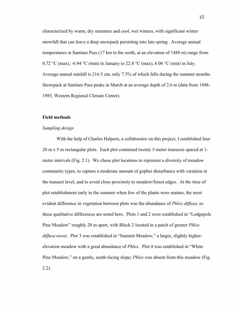
With the help of Charles Halpern, a collaborator on this project, I established four

20 m x 5 m rectangular plots. Each plot contained twenty 5-meter transects spaced at 1-

meter intervals (Fig. 2.1). We chose plot locations to represent a diversity of meadow

community types, to capture a moderate amount of gopher disturbance with variation at

the transect level, and to avoid close proximity to meadow/forest edges. At the time of

plot establishment early in the summer when few of the plants were mature, the most

evident difference in vegetation between plots was the abundance of Phlox diffusa, so

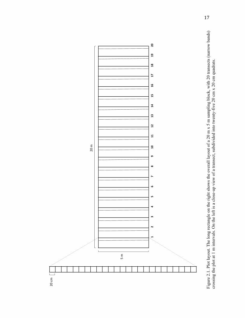
these qualitative differences are noted here. Plots 1 and 2 were established in “Lodgepole

Pine Meadow” roughly 20 m apart, with Block 2 located in a patch of greater Phlox

diffusa cover. Plot 3 was established in “Summit Meadow,” a larger, slightly higher-

elevation meadow with a great abundance of Phlox. Plot 4 was established in “White

Pine Meadow,” on a gentle, south-facing slope; Phlox was absent from this meadow (Fig.

2.2).

16

After choosing the general location and orientation of each plot, one plot corner

was established at the landing point of a chaining pin tossed blindly into the air. We

surveyed a rectangle from this starting corner, verifying the accuracy of the rectangle side

lengths to within +/- 1% of the expected perimeter. We marked each plot corner with a

~0.7 m segment of PVC pipe hammered into the ground and placed pin flags at 1-m

intervals along the long sides of each plot to mark the endpoints of the transects. When

pin flags occasionally disappeared throughout the summer due to elk trampling or other

natural disturbance, I relocated them by measuring between the two adjacent flags.

Each five-meter transect was sampled with 25 contiguous quadrats (20 cm x 20

cm, Fig. 2.1). I measured the extent of gopher disturbance and vegetation as visual

estimates of percent cover (100% being the total area of a quadrat square, 400 cm2).

Percent cover is a commonly used metric for ground surface variables as well as

vegetation measurements, particularly in systems such as this one in which the presence

of bunchgrasses and clonal plants makes counts of individuals impractical (e.g. Sherrod

et al. 2005, Jones et al. 2008, McCain et al. 2010). I made all cover estimates myself,

with my field assistant, Sarah Koe, recording data. I calibrated my estimates at the

beginning of the summer by measuring and calculating the area of various plants with a

centimeter ruler, and re-calibrated throughout the summer to ensure consistent estimation.

I estimated cover values <1% as either 0.5% or 0.1%, values between 1 and 10% to the

nearest 1%, and values >10% to the nearest 5%.

17

Figu

re 2

.1. P

lot l

ayou

t. Th

e lo

ng re

ctan

gle

on th

e rig

ht sh

ows t

he o

vera

ll la

yout

of a

20

m x

5 m

sam

plin

g bl

ock,

with

20

trans

ects

(nar

row

ban

ds)

cros

sing

the

plot

at 1

m in

terv

als.

On

the

left

is a

clo

se-u

p vi

ew o

f a tr

anse

ct, s

ubdi

vide

d in

to tw

enty

-fiv

e 20

cm

x 2

0 cm

qua

drat

s. ! !

1!2!

3!4!

5!6!

7!8!

9!10!

11!

12!

13!

14!

15!

16!

17!

18!

19!

!20!

20#cm#

5#m#

20#m

#

18

Figure 2.2. Aerial photo of Bunchgrass Ridge with sampling locations marked by plot number. The square or rectangular openings in the center of the photo are 1-ha experimental plots from which trees were removed in 2006.

Timing of sampling

I sampled all transects for gopher disturbance between June 20 and 30, 2011, and

for vegetation between July 7 and August 12, 2011. This temporal separation between

disturbance and vegetation sampling allowed us to measure disturbance soon after snow

melt, when most plants had not yet emerged and gopher disturbance was most evident,

and then to return for vegetation sampling when the plants were mature. The order in

which we sampled the four plots for ground conditions and vegetation was determined by

plant phenology.

19

Disturbance sampling

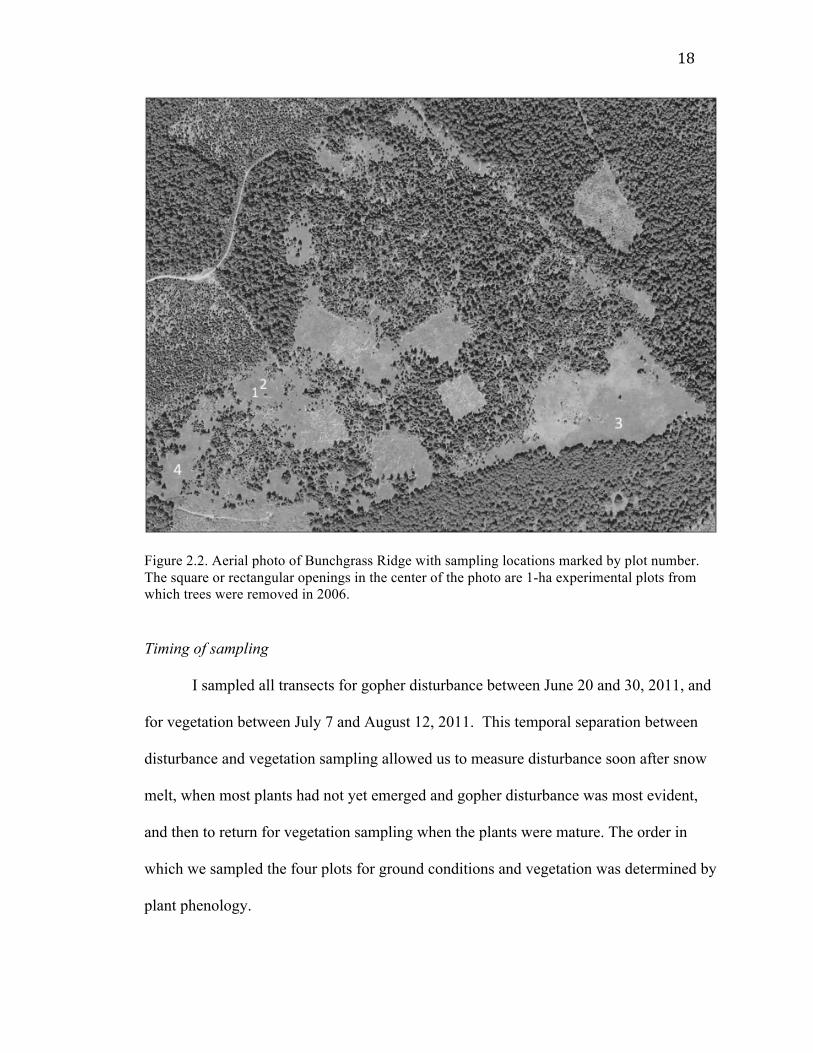
Gopher disturbance categories included fresh mound, old mound, casting, tunnel,

and hole. Fresh mounds were defined as mounds created during the current growing

season, consisting of loose, un-compacted soil with no vegetation cover (Fig. 2.3). All

other mounds – which showed evidence of compaction or weathering, and typically had

some vegetation cover – were defined as old mounds (Figs. 2.3-4).

Figure 2.3. Fresh mound (front) adjacent to old mound (back). Photo by Charles Halpern.

20

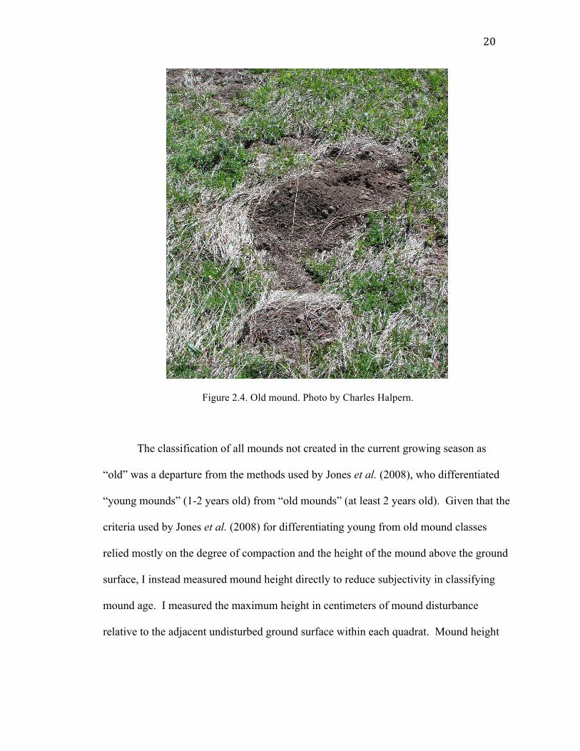
Figure 2.4. Old mound. Photo by Charles Halpern.

The classification of all mounds not created in the current growing season as

“old” was a departure from the methods used by Jones et al. (2008), who differentiated

“young mounds” (1-2 years old) from “old mounds” (at least 2 years old). Given that the

criteria used by Jones et al. (2008) for differentiating young from old mound classes

relied mostly on the degree of compaction and the height of the mound above the ground

surface, I instead measured mound height directly to reduce subjectivity in classifying

mound age. I measured the maximum height in centimeters of mound disturbance

relative to the adjacent undisturbed ground surface within each quadrat. Mound height

21

measurements were significantly correlated with mound cover, however, so they were not

used in the analysis (Kendall’s rank correlation, tau = 0.3359, z = 12.7445, p < 2.2e-16).

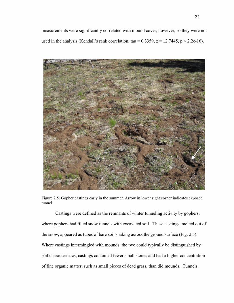
Figure 2.5. Gopher castings early in the summer. Arrow in lower right corner indicates exposed tunnel.

Castings were defined as the remnants of winter tunneling activity by gophers,

where gophers had filled snow tunnels with excavated soil. These castings, melted out of

the snow, appeared as tubes of bare soil snaking across the ground surface (Fig. 2.5).

Where castings intermingled with mounds, the two could typically be distinguished by

soil characteristics; castings contained fewer small stones and had a higher concentration

of fine organic matter, such as small pieces of dead grass, than did mounds. Tunnels,

22

which also likely resulted from winter tunneling activity between the ground surface and

the snow, were defined as exposed hollow tunnels not backfilled with soil. Holes were

defined as openings leading to subterranean tunnels. New disturbances (fresh mounds or

holes) observed at the time of vegetation sampling were recorded, but were remarkably

infrequent, and were not considered in the analyses of disturbance-vegetation

relationships.

During ground surface and disturbance sampling I also measured percent cover of

Claytonia lanceolata, an ephemeral herb that flowers soon after snow melt and senesces

early in the summer, knowing that it would be largely absent by the time we began

vegetation sampling.

Vegetation sampling

I identified all plant species in or above each quadrat and estimated foliar cover of

each species as a vertical projection into the quadrat. Because of overlap among species,

total cover of all species in a quadrat could sum to more than 100%. I identified all

plants to species, with the exception of Fragaria spp. (which included F. vesca and F.

virginiana) and a seedling of Acer sp. When I could not identify a plant in the field, I

took detailed notes and photographs and/or collected a specimen from outside the plot,

and identified it later with the help of herbarium specimens or other reference materials.

Nomenclature follows Hitchcock & Cronquist (1973).

23

Statistical methods

Data aggregation and summary

I used the R statistical package (R Development Core Team 2011) for all

analyses. I calculated total cover of forbs, graminoids, and all plants, as well as total

gopher disturbance, for each transect (mean of 25 quadrats), and calculated the ratio of

forb to graminoid cover at the transect level. I also calculated total percent cover of forbs

with Phlox diffusa excluded. Although Jones et al. (2008) treated Phlox as a forb, it is

more appropriately defined as a sub-shrub given its woody base and branches (Hitchcock

& Cronquist 1973).

For each quadrat and transect I calculated species richness as the total number of

species counted. I calculated an index of species evenness for each transect, using the

modified Hill’s ratio recommended by Alatalo (1981): (N2 – 1)/(N1 – 1), where N1 and N2

are the Hill numbers of order 1 and 2, estimates of the effective number of species with

different weights placed on rare species (Hill 1973). With pi as the ratio of the total

percent cover of the ith species to the total cover of all plants in the sample,

N! = exp  (− 𝑝! ∗ ln  (𝑝!))

N! =1𝑝!!

(Hill numbers calculated with vegan package, Oksanen et al. 2011). I also

calculated an index of mean community heterogeneity for each transect by taking the

mean of the Bray-Curtis dissimilarity (Bray & Curtis 1957; ecodist package, Goslee &

Urban 2007) of all pairs of quadrats within the transect.

24

Statistical models and tests

I investigated relationships between disturbance and vegetation using linear

mixed-effects models (lme4 package, Bates et al. 2011), treating disturbance variables as

fixed effects and plot as a random effect to account for potential correlation of errors

within plots. Each model used the maximal random-effects structure justified by the

data. For some models a random-intercept term was sufficient, but others required a

random slope and random intercept because the addition of a random slope significantly

improved the fit of the model. I obtained p-values for fixed effects (disturbance variables)

using the pamer.fnc() function (LMERConvenienceFunctions package, Tremblay 2011),

which computes upper- and lower-bound p-values for the analysis of variance for each

fixed effect according to the range of possible degrees of freedom. The upper- and

lower-bound p-values generally differed by less than 0.001, so for simplicity I report only

the more conservative upper-bound p-value and the corresponding degrees of freedom

(see Appendix A for further discussion of mixed-effects models and the computation of

p-values).

For total disturbance, I fitted a mixed-effects model for each of several plant

response variables at the transect scale: total plant cover, total forb cover, total graminoid

cover, total forb cover with Phlox excluded, forb/graminoid ratio, species richness,

evenness, and community heterogeneity. Because I might expect a peaked, unimodal

relationship between richness and disturbance according to the Intermediate Disturbance

Hypothesis, I also modeled richness as a quadratic function of disturbance and compared

this to the linear model with a likelihood-ratio test. To assess the individual effects of old

mound and casting (the two most common forms of gopher disturbance), I modeled each

25

of the plant response variables as a function of old mound and casting as additive fixed

effects, with plot as a random effect. I tested for correlation between cover of mounds

and castings at quadrat and transect scales using a Kendall’s rank correlation test because

the data did not meet the requirements of normality.

The spatially explicit layout of the transects and quadrats within plots also

allowed investigation of the spatial autocorrelation of cover of disturbance and plant

variables. To understand the spatial correlation structure of the main variables of interest

at the quadrat scale, I developed correlograms (0.2-10 m) for cover of total disturbance,

old mounds, castings, total plants, total forbs, and total graminoids. Correlograms were

produced using the spatial package (Venables & Ripley 2002).

26

Chapter 3

Field Results

Disturbance conditions

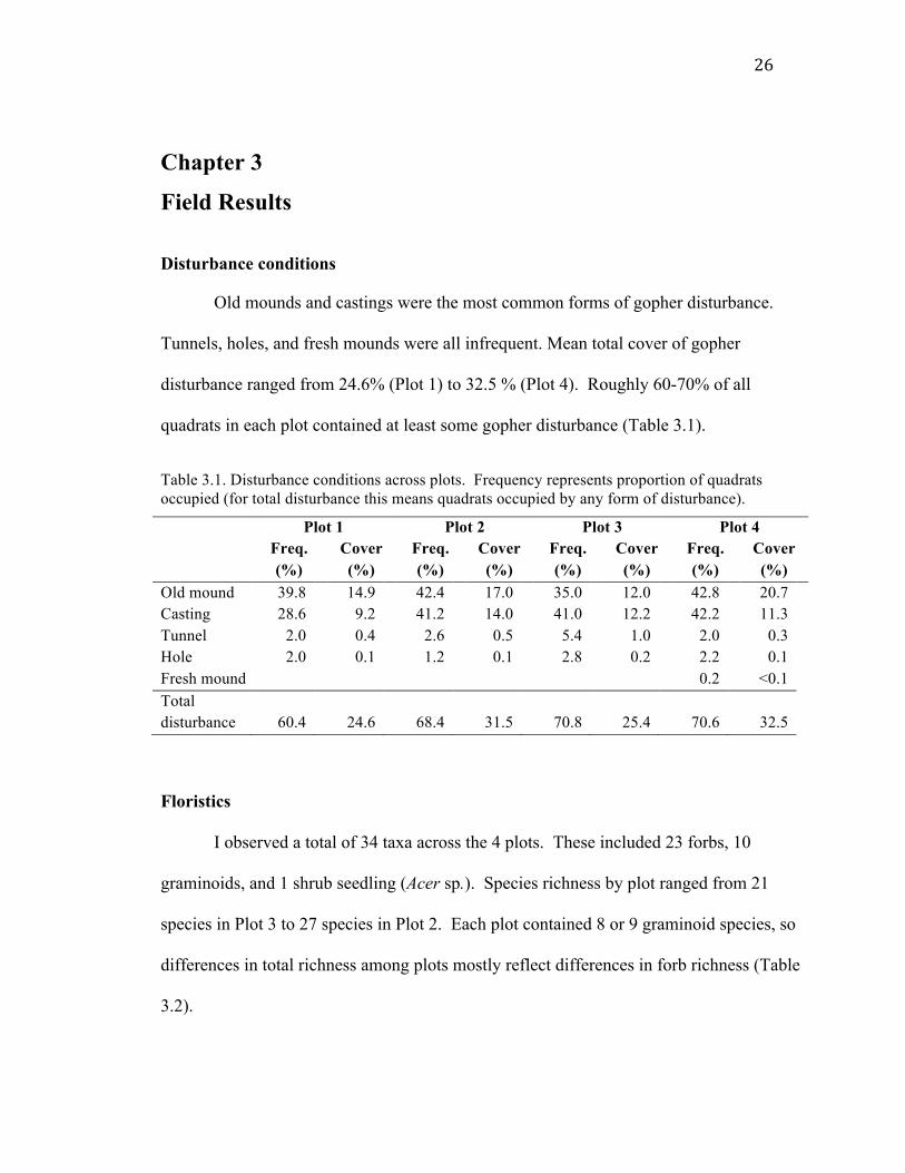
Old mounds and castings were the most common forms of gopher disturbance.

Tunnels, holes, and fresh mounds were all infrequent. Mean total cover of gopher

disturbance ranged from 24.6% (Plot 1) to 32.5 % (Plot 4). Roughly 60-70% of all

quadrats in each plot contained at least some gopher disturbance (Table 3.1).

Table 3.1. Disturbance conditions across plots. Frequency represents proportion of quadrats occupied (for total disturbance this means quadrats occupied by any form of disturbance).

Plot 1 Plot 2 Plot 3 Plot 4 Freq.

(%) Cover (%)

Freq. (%)

Cover (%)

Freq. (%)

Cover (%)

Freq. (%)

Cover (%)

Old mound 39.8 14.9 42.4 17.0 35.0 12.0 42.8 20.7 Casting 28.6 9.2 41.2 14.0 41.0 12.2 42.2 11.3 Tunnel 2.0 0.4 2.6 0.5 5.4 1.0 2.0 0.3 Hole 2.0 0.1 1.2 0.1 2.8 0.2 2.2 0.1 Fresh mound 0.2 <0.1 Total disturbance

60.4

24.6

68.4

31.5

70.8

25.4

70.6

32.5

Floristics

I observed a total of 34 taxa across the 4 plots. These included 23 forbs, 10

graminoids, and 1 shrub seedling (Acer sp.). Species richness by plot ranged from 21

species in Plot 3 to 27 species in Plot 2. Each plot contained 8 or 9 graminoid species, so

differences in total richness among plots mostly reflect differences in forb richness (Table

3.2).

27

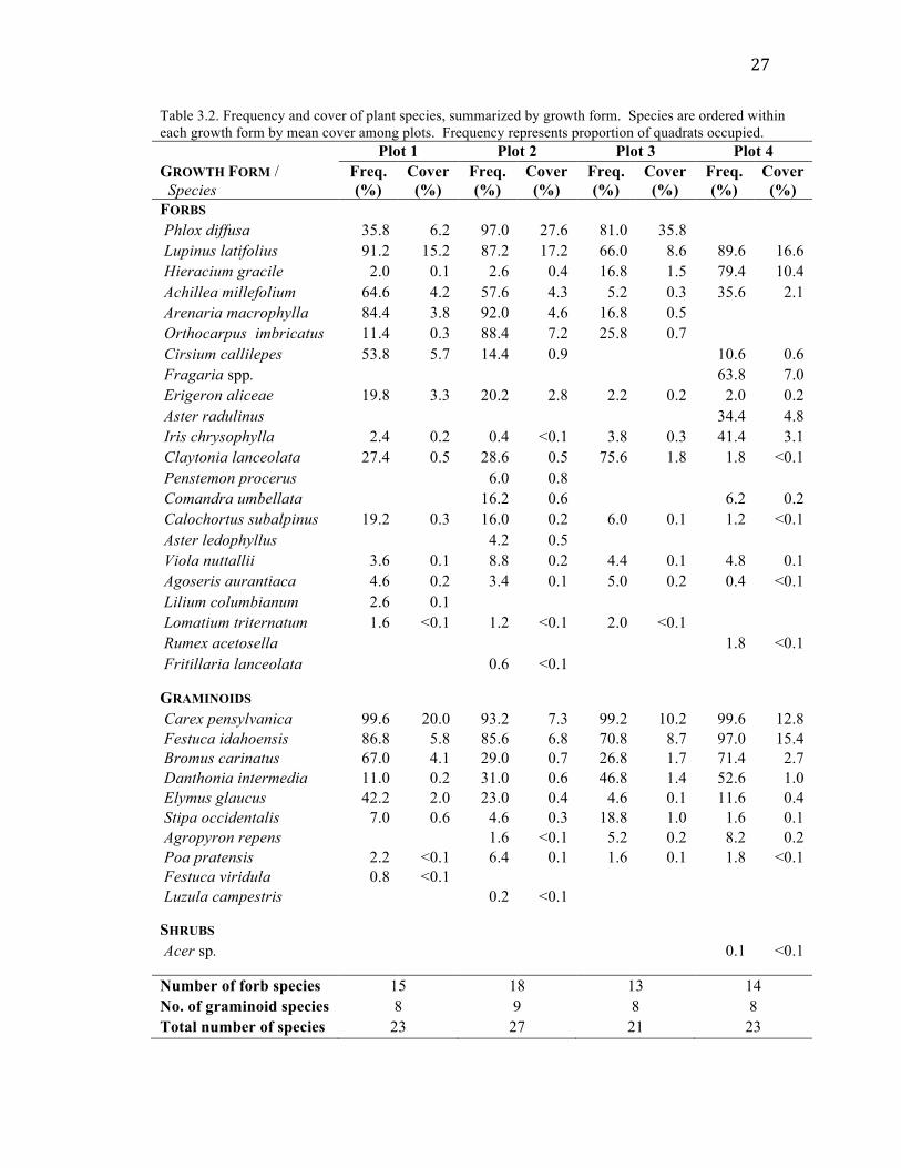
Table 3.2. Frequency and cover of plant species, summarized by growth form. Species are ordered within each growth form by mean cover among plots. Frequency represents proportion of quadrats occupied. Plot 1 Plot 2 Plot 3 Plot 4 GROWTH FORM / Species

Freq. (%)

Cover (%)

Freq. (%)

Cover (%)

Freq. (%)

Cover (%)

Freq. (%)

Cover (%)

FORBS Phlox diffusa 35.8 6.2 97.0 27.6 81.0 35.8 Lupinus latifolius 91.2 15.2 87.2 17.2 66.0 8.6 89.6 16.6 Hieracium gracile 2.0 0.1 2.6 0.4 16.8 1.5 79.4 10.4 Achillea millefolium 64.6 4.2 57.6 4.3 5.2 0.3 35.6 2.1 Arenaria macrophylla 84.4 3.8 92.0 4.6 16.8 0.5 Orthocarpus imbricatus 11.4 0.3 88.4 7.2 25.8 0.7 Cirsium callilepes 53.8 5.7 14.4 0.9 10.6 0.6 Fragaria spp. 63.8 7.0 Erigeron aliceae 19.8 3.3 20.2 2.8 2.2 0.2 2.0 0.2 Aster radulinus 34.4 4.8 Iris chrysophylla 2.4 0.2 0.4 <0.1 3.8 0.3 41.4 3.1 Claytonia lanceolata 27.4 0.5 28.6 0.5 75.6 1.8 1.8 <0.1 Penstemon procerus 6.0 0.8 Comandra umbellata 16.2 0.6 6.2 0.2 Calochortus subalpinus 19.2 0.3 16.0 0.2 6.0 0.1 1.2 <0.1 Aster ledophyllus 4.2 0.5 Viola nuttallii 3.6 0.1 8.8 0.2 4.4 0.1 4.8 0.1 Agoseris aurantiaca 4.6 0.2 3.4 0.1 5.0 0.2 0.4 <0.1 Lilium columbianum 2.6 0.1 Lomatium triternatum 1.6 <0.1 1.2 <0.1 2.0 <0.1 Rumex acetosella 1.8 <0.1 Fritillaria lanceolata 0.6 <0.1 GRAMINOIDS Carex pensylvanica 99.6 20.0 93.2 7.3 99.2 10.2 99.6 12.8 Festuca idahoensis 86.8 5.8 85.6 6.8 70.8 8.7 97.0 15.4 Bromus carinatus 67.0 4.1 29.0 0.7 26.8 1.7 71.4 2.7 Danthonia intermedia 11.0 0.2 31.0 0.6 46.8 1.4 52.6 1.0 Elymus glaucus 42.2 2.0 23.0 0.4 4.6 0.1 11.6 0.4 Stipa occidentalis 7.0 0.6 4.6 0.3 18.8 1.0 1.6 0.1 Agropyron repens 1.6 <0.1 5.2 0.2 8.2 0.2 Poa pratensis 2.2 <0.1 6.4 0.1 1.6 0.1 1.8 <0.1 Festuca viridula 0.8 <0.1 Luzula campestris 0.2 <0.1 SHRUBS Acer sp. 0.1 <0.1 Number of forb species 15 18 13 14 No. of graminoid species 8 9 8 8 Total number of species 23 27 21 23

28

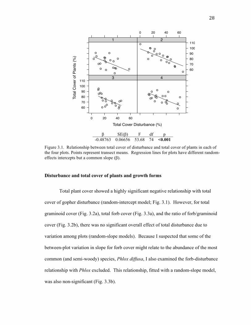
β SE(β) F df p

-0.48763 0.06656 53.68 74 <0.001

Figure 3.1. Relationship between total cover of disturbance and total cover of plants in each of the four plots. Points represent transect means. Regression lines for plots have different random-effects intercepts but a common slope (β).

Disturbance and total cover of plants and growth forms

Total plant cover showed a highly significant negative relationship with total

cover of gopher disturbance (random-intercept model; Fig. 3.1). However, for total

graminoid cover (Fig. 3.2a), total forb cover (Fig. 3.3a), and the ratio of forb/graminoid

cover (Fig. 3.2b), there was no significant overall effect of total disturbance due to

variation among plots (random-slope models). Because I suspected that some of the

between-plot variation in slope for forb cover might relate to the abundance of the most

common (and semi-woody) species, Phlox diffusa, I also examined the forb-disturbance

relationship with Phlox excluded. This relationship, fitted with a random-slope model,

was also non-significant (Fig. 3.3b).

Total Cover Disturbance (%)

Tota

l Cov

er o

f Pla

nts

(%)

60708090

100110

0 20 40 60

●

●

●●●

●

●

●

●

●

●

●

●

●●●●

● ●

●

3

●

●●

●

●

●

●

●

●

●●

●

●

●

●

●

●

●

●

●

4

●

●

●

●

●

●

●●

●

●

●

●

●

●●●

●

●●

●

1

0 20 40 60

60708090100110●

●

●

●

●

●

●

●●●

●

●

●

●

●●

●●

●●

2

29

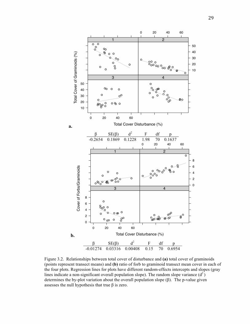
a. β SE(β) d2 F df p

-0.2654 0.1869 0.1228 1.98 70 0.1637

b. β SE(β) d2 F df p

-0.01274 0.03316 0.00408 0.15 70 0.6954 Figure 3.2. Relationships between total cover of disturbance and (a) total cover of graminoids (points represent transect means) and (b) ratio of forb to graminoid transect mean cover in each of the four plots. Regression lines for plots have different random-effects intercepts and slopes (gray lines indicate a non-significant overall population slope). The random slope variance (d2 ) determines the by-plot variation about the overall population slope (β). The p-value given assesses the null hypothesis that true β is zero.

Total Cover Disturbance (%)

Tota

l Cov

er o

f Gra

min

oids

(%)

10

20

30

40

50

0 20 40 60

●

● ●●

●

●

●

● ●●●●

●●● ●● ●

●

●

3

●●

●

●

●

●

●●●

●

●

●

●

●●

● ●

●

●

●

4

●●

●●●●

●●

●● ●●

●

●

●●

●●●

●

1

0 20 40 60

10

20

30

40

50

●●● ●

●

●●

● ●●

●●

●●●●●●●●

2

Total Cover Disturbance (%)

Cov

er o

f For

bs/G

ram

inoi

ds

0

2

4

6

8

0 20 40 60

●● ●●

●

●

●

●●

●

●

●●

●● ●● ●

●●

3

●●

●

●●●

● ●

●●●● ●●●

●●●●●

4●● ● ●●

●●

●

●●

●●● ●● ●●

●●

●

1

0 20 40 60

0

2

4

6

8

●●

● ●

●

●●

●●

●

●

●

●

●●

●●●●●

2

30

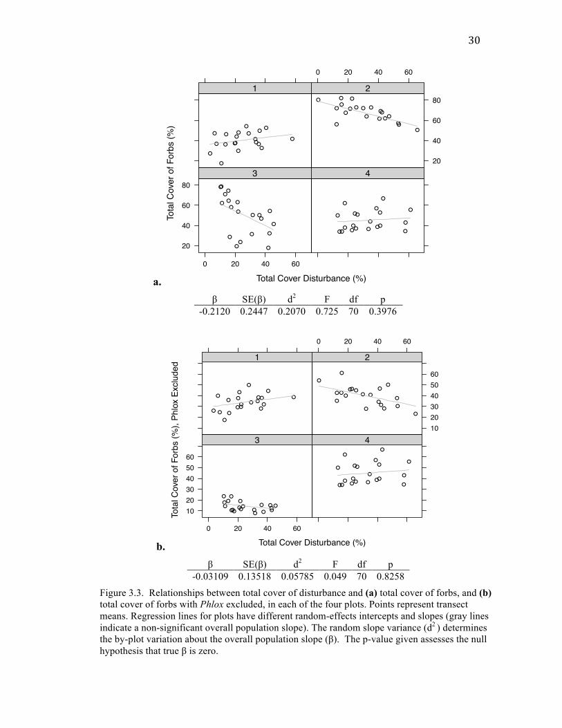
a. β SE(β) d2 F df p

-0.2120 0.2447 0.2070 0.725 70 0.3976

b. β SE(β) d2 F df p

-0.03109 0.13518 0.05785 0.049 70 0.8258

Figure 3.3. Relationships between total cover of disturbance and (a) total cover of forbs, and (b) total cover of forbs with Phlox excluded, in each of the four plots. Points represent transect means. Regression lines for plots have different random-effects intercepts and slopes (gray lines indicate a non-significant overall population slope). The random slope variance (d2 ) determines the by-plot variation about the overall population slope (β). The p-value given assesses the null hypothesis that true β is zero.

Total Cover Disturbance (%)

Tota

l Cov

er o

f For

bs (%

)

20

40

60

80

0 20 40 60

●

●●●

●

●

●

●

●

●

●

●

●

●●●●

●

●●

3

●

●●

● ●

● ●●

●●

●● ●

●

●

●

●●●●

4●

●

●

●

●

● ●●

●

●

●●

●●

● ●●

●●●

1

0 20 40 60

20

40

60

80●

●

●●

●

●●

●●●

●

●●

●

●●

●●

●●

2

Total Cover Disturbance (%)

Tota

l Cov

er o

f For

bs (%

), Ph

lox

Excl

uded

102030405060

0 20 40 60

●● ●●

●

●●

●●

●

●●

●●

●●●

●●●

3

●

●●

● ●

● ●●

●

●●

● ●

●

●

●

●●●●

4

●

● ●●●

●

●

●

●

●

●●

●●

●●

●

●

●

●

1

0 20 40 60

102030405060

●

●

●●

●

●

●

●●

●

●

●

●●

●

●

●●●

●

2

31

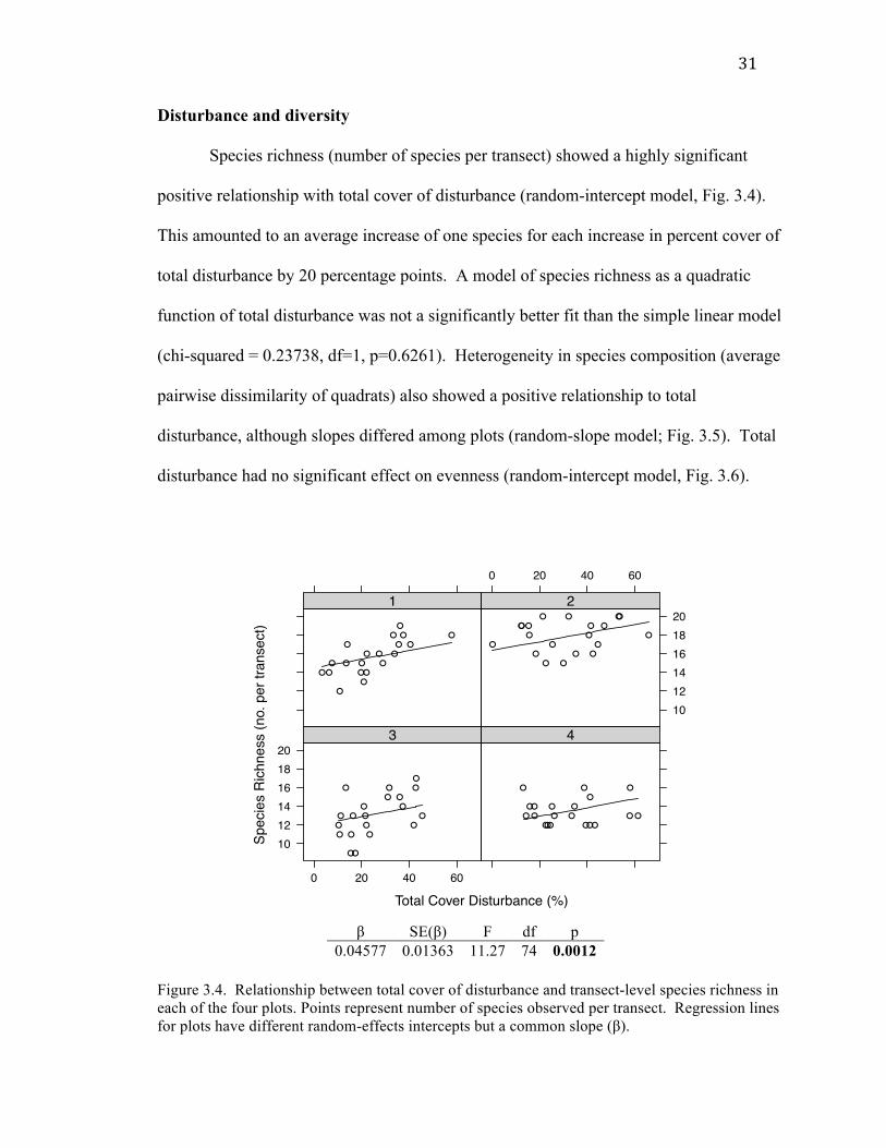
Disturbance and diversity

Species richness (number of species per transect) showed a highly significant

positive relationship with total cover of disturbance (random-intercept model, Fig. 3.4).

This amounted to an average increase of one species for each increase in percent cover of

total disturbance by 20 percentage points. A model of species richness as a quadratic

function of total disturbance was not a significantly better fit than the simple linear model

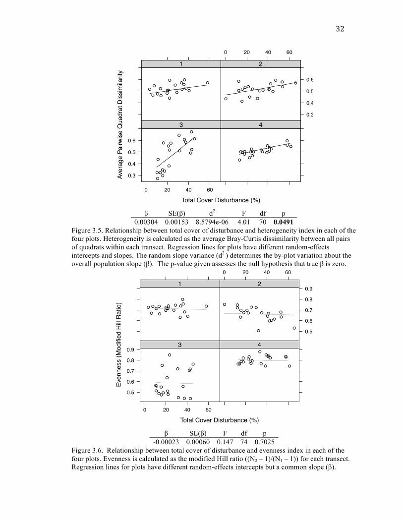
(chi-squared = 0.23738, df=1, p=0.6261). Heterogeneity in species composition (average

pairwise dissimilarity of quadrats) also showed a positive relationship to total

disturbance, although slopes differed among plots (random-slope model; Fig. 3.5). Total

disturbance had no significant effect on evenness (random-intercept model, Fig. 3.6).

β SE(β) F df p

0.04577 0.01363 11.27 74 0.0012

Figure 3.4. Relationship between total cover of disturbance and transect-level species richness in each of the four plots. Points represent number of species observed per transect. Regression lines for plots have different random-effects intercepts but a common slope (β).

Total Cover Disturbance (%)

Spec

ies

Ric

hnes

s (n

o. p

er tr

anse

ct)

101214161820

0 20 40 60

●

●

●

●

●

●

●

●

●

●●

●

●

●

●

●

●

●

●

●

3

●

●

● ●

●

● ●

●●

●

●

● ●

●●

●

●

●

●

●

4

●

●

●

●●●

●

●

●

● ●

●

●

●● ●

●

●

●

●

1

0 20 40 60

101214161820

●

●●

●

●

●

●

● ●

● ●

●

●

●

● ●

●

●

●

●

2

32

β SE(β) d2 F df p

0.00304 0.00153 8.5794e-06 4.01 70 0.0491 Figure 3.5. Relationship between total cover of disturbance and heterogeneity index in each of the four plots. Heterogeneity is calculated as the average Bray-Curtis dissimilarity between all pairs of quadrats within each transect. Regression lines for plots have different random-effects intercepts and slopes. The random slope variance (d2 ) determines the by-plot variation about the overall population slope (β). The p-value given assesses the null hypothesis that true β is zero.

β SE(β) F df p

-0.00023 0.00060 0.147 74 0.7025 Figure 3.6. Relationship between total cover of disturbance and evenness index in each of the four plots. Evenness is calculated as the modified Hill ratio ((N2 – 1)/(N1 – 1)) for each transect. Regression lines for plots have different random-effects intercepts but a common slope (β).

Total Cover Disturbance (%)

Aver

age

Pairw

ise

Qua

drat

Dis

sim

ilarit

y

0.3

0.4

0.5

0.6

0 20 40 60

●

●

●

●●

●

●

●

●●●

●●

●

● ●●

●

●●

3

●●

●●

●●

●

●

●

●●

●

●

●●

●●●

●●

4

●

●●

●

●●

●●●

●●●● ●

● ●●

●●

●

1

0 20 40 60

0.3

0.4

0.5

0.6

●

●

●●

●

●● ●

●

●

● ●●

●●

●

●

●

●

●

2

Total Cover Disturbance (%)

Even

ness

(Mod

ified

Hill

Rat

io)

0.5

0.6

0.7

0.8

0.9

0 20 40 60

●

●

●

●

●

●

●●

●●

●●●

●

● ●●

●

●●

3

●

●●

●

●

●

●

●

●●

●

●●

●●●

●

●●●

4

●● ●●

●●

●

●

●●

●●

●

●

●

●

●

●●

●

1

0 20 40 60

0.5

0.6

0.7

0.8

0.9

● ●●

●

●

●●●

●

●

●

●

●●●

●

●●

●●

2

33

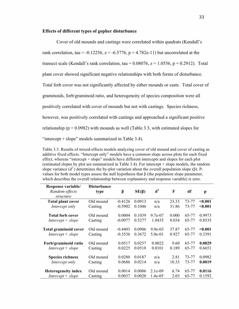
Effects of different types of gopher disturbance

Cover of old mounds and castings were correlated within quadrats (Kendall’s

rank correlation, tau = -0.12256, z = -6.5776, p = 4.782e-11) but uncorrelated at the

transect scale (Kendall’s rank correlation, tau = 0.08076, z = 1.0556, p = 0.2912). Total

plant cover showed significant negative relationships with both forms of disturbance.

Total forb cover was not significantly affected by either mounds or casts. Total cover of

graminoids, forb/graminoid ratio, and heterogeneity of species composition were all

positively correlated with cover of mounds but not with castings. Species richness,

however, was positively correlated with castings and approached a significant positive

relationship (p = 0.0982) with mounds as well (Table 3.3, with estimated slopes for

“intercept + slope” models summarized in Table 3.4).

Table 3.3. Results of mixed-effects models analyzing cover of old mound and cover of casting as additive fixed effects. “Intercept only” models have a common slope across plots for each fixed effect, whereas “intercept + slope” models have different intercepts and slopes for each plot (estimated slopes by plot are summarized in Table 3.4). For intercept + slope models, the random slope variance (d2 ) determines the by-plot variation about the overall population slope (β). P-values for both model types assess the null hypothesis that β (the population slope parameter, which describes the overall relationship between explanatory and response variable) is zero.

Response variable/ Random-effects

structure

Disturbance type

β

SE(β)

d2

F

df

p

Total plant cover Intercept only

Old mound -0.4126 0.0913 n/a 23.33 73-77 <0.001 Casting -0.5902 0.1046 n/a 31.86 73-77 <0.001

Total forb cover Intercept + slope

Old mound 0.0004 0.1039 9.7e-07 0.000 65-77 0.9973 Casting -0.0977 0.5277 1.0435 0.034 65-77 0.8535

Total graminoid cover

Intercept + slope Old mound -0.4403 0.0906 9.9e-03 37.87 65-77 <0.001 Casting -0.3536 0.3672 5.0e-01 0.927 65-77 0.3391

Forb/graminoid ratio

Intercept + slope Old mound 0.0517 0.0257 0.0022 9.60 65-77 0.0029 Casting 0.0225 0.0518 0.0101 0.189 65-77 0.6651

Species richness

Intercept only Old mound 0.0280 0.0187 n/a 2.81 73-77 0.0982 Casting 0.0686 0.0214 n/a 10.33 73-77 0.0019

Heterogeneity index

Intercept + slope Old mound 0.0014 0.0006 2.1e-09 6.74 65-77 0.0116 Casting 0.0037 0.0020 1.4e-05 2.03 65-77 0.1592

34

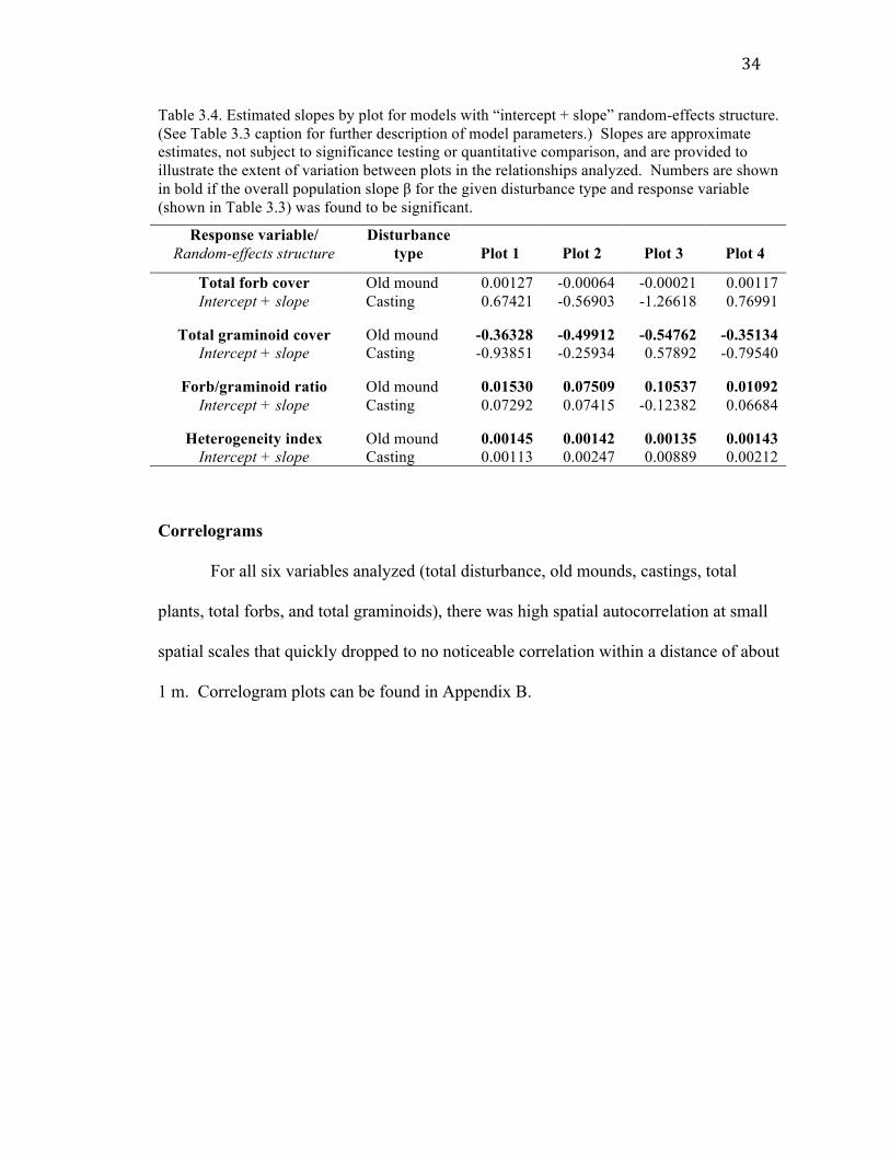
Table 3.4. Estimated slopes by plot for models with “intercept + slope” random-effects structure. (See Table 3.3 caption for further description of model parameters.) Slopes are approximate estimates, not subject to significance testing or quantitative comparison, and are provided to illustrate the extent of variation between plots in the relationships analyzed. Numbers are shown in bold if the overall population slope β for the given disturbance type and response variable (shown in Table 3.3) was found to be significant.

Response variable/ Random-effects structure

Disturbance type

Plot 1

Plot 2

Plot 3

Plot 4

Total forb cover Intercept + slope

Old mound 0.00127 -0.00064 -0.00021 0.00117 Casting 0.67421 -0.56903 -1.26618 0.76991

Total graminoid cover

Intercept + slope Old mound -0.36328 -0.49912 -0.54762 -0.35134 Casting -0.93851 -0.25934 0.57892 -0.79540

Forb/graminoid ratio

Intercept + slope Old mound 0.01530 0.07509 0.10537 0.01092 Casting 0.07292 0.07415 -0.12382 0.06684

Heterogeneity index

Intercept + slope Old mound 0.00145 0.00142 0.00135 0.00143 Casting 0.00113 0.00247 0.00889 0.00212

Correlograms

For all six variables analyzed (total disturbance, old mounds, castings, total

plants, total forbs, and total graminoids), there was high spatial autocorrelation at small

spatial scales that quickly dropped to no noticeable correlation within a distance of about

1 m. Correlogram plots can be found in Appendix B.

35

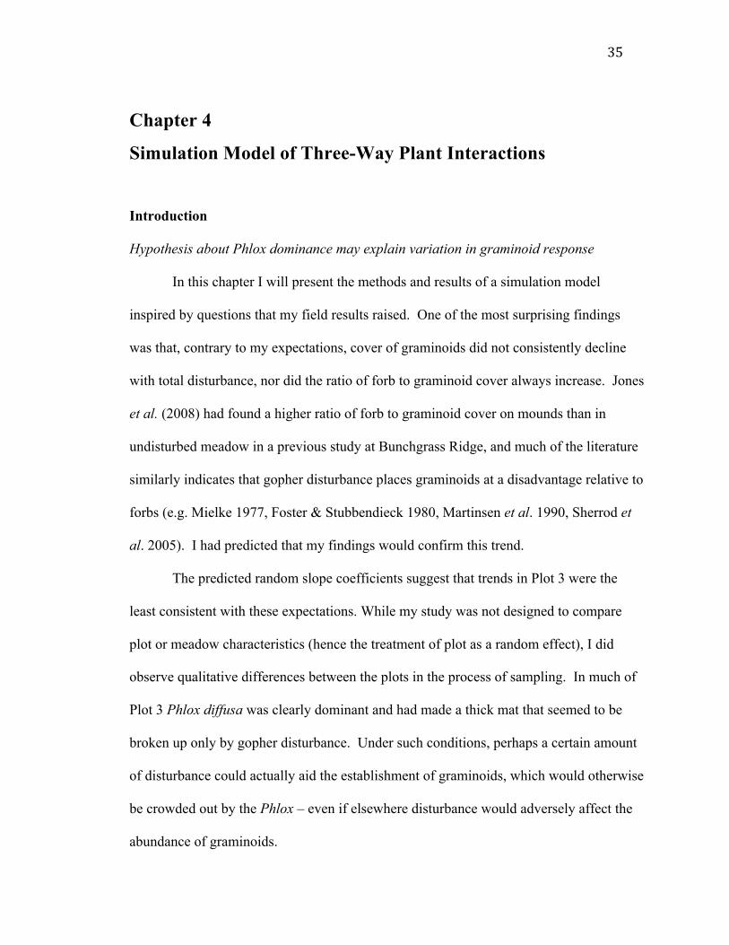
Chapter 4

Simulation Model of Three-Way Plant Interactions

Introduction

Hypothesis about Phlox dominance may explain variation in graminoid response

In this chapter I will present the methods and results of a simulation model

inspired by questions that my field results raised. One of the most surprising findings

was that, contrary to my expectations, cover of graminoids did not consistently decline

with total disturbance, nor did the ratio of forb to graminoid cover always increase. Jones

et al. (2008) had found a higher ratio of forb to graminoid cover on mounds than in

undisturbed meadow in a previous study at Bunchgrass Ridge, and much of the literature

similarly indicates that gopher disturbance places graminoids at a disadvantage relative to

forbs (e.g. Mielke 1977, Foster & Stubbendieck 1980, Martinsen et al. 1990, Sherrod et

al. 2005). I had predicted that my findings would confirm this trend.

The predicted random slope coefficients suggest that trends in Plot 3 were the

least consistent with these expectations. While my study was not designed to compare

plot or meadow characteristics (hence the treatment of plot as a random effect), I did

observe qualitative differences between the plots in the process of sampling. In much of

Plot 3 Phlox diffusa was clearly dominant and had made a thick mat that seemed to be

broken up only by gopher disturbance. Under such conditions, perhaps a certain amount

of disturbance could actually aid the establishment of graminoids, which would otherwise

be crowded out by the Phlox – even if elsewhere disturbance would adversely affect the

abundance of graminoids.

36

A modeling approach to exploring the Phlox hypothesis

The simulation model described in this chapter was designed to test my Phlox

hypothesis. Was it feasible for the presence of a highly competitive plant such as Phlox

to mediate the nature of the relationship between disturbance and the abundance of

another plant species? Could I construct a model in which a graminoid-like species

declined with increasing disturbance when Phlox was not present, but increased in

response to increasing disturbance when Phlox was added to the system?

In more general terms, this model can be seen as an extension of the basic

conceptual framework behind justifications of the Intermediate Disturbance Hypothesis,

which classifies organisms as either good colonizers or good competitors (Connell 1978).

Most studies of gopher disturbance categorize plants in a similarly binary fashion: forbs

vs. graminoids, annuals vs. perennials (Martinsen et al. 1990, Rogers & Hartnett 2001,

Jones et al. 2008). Here I complicate this basic concept of trade-offs by exploring the

interactions of three types of plants located along a spectrum from colonization ability to

competitive ability, with forbs considered the best colonizers, Phlox the best competitor,

and graminoids somewhere in between.

Modeling methods

Description of the model

The basic structure of this model was inspired by other grid-based spatially

explicit models of gopher-plant interactions (Moloney & Levin 1996, Seabloom &

Reichman 2001). The model universe consists of a square grid of 100x100 cells, with

periodic boundary conditions to avoid edge effects. The presence or absence of each plant

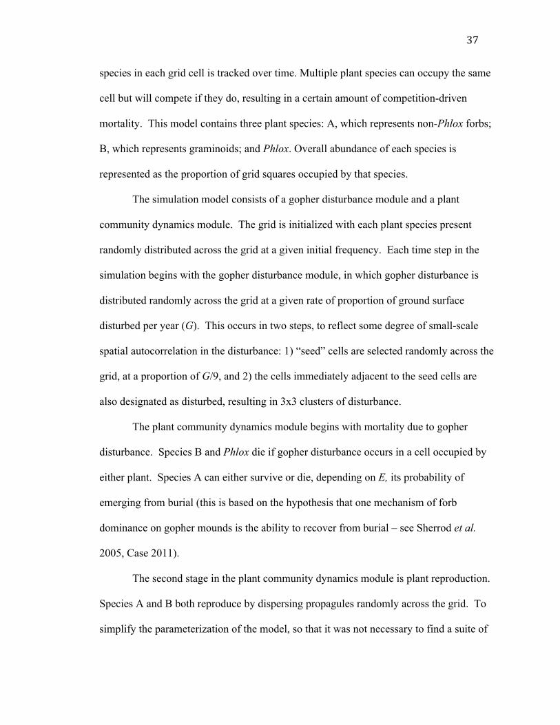
37

species in each grid cell is tracked over time. Multiple plant species can occupy the same

cell but will compete if they do, resulting in a certain amount of competition-driven

mortality. This model contains three plant species: A, which represents non-Phlox forbs;

B, which represents graminoids; and Phlox. Overall abundance of each species is

represented as the proportion of grid squares occupied by that species.

The simulation model consists of a gopher disturbance module and a plant

community dynamics module. The grid is initialized with each plant species present

randomly distributed across the grid at a given initial frequency. Each time step in the

simulation begins with the gopher disturbance module, in which gopher disturbance is

distributed randomly across the grid at a given rate of proportion of ground surface

disturbed per year (G). This occurs in two steps, to reflect some degree of small-scale

spatial autocorrelation in the disturbance: 1) “seed” cells are selected randomly across the

grid, at a proportion of G/9, and 2) the cells immediately adjacent to the seed cells are

also designated as disturbed, resulting in 3x3 clusters of disturbance.

The plant community dynamics module begins with mortality due to gopher

disturbance. Species B and Phlox die if gopher disturbance occurs in a cell occupied by

either plant. Species A can either survive or die, depending on E, its probability of

emerging from burial (this is based on the hypothesis that one mechanism of forb

dominance on gopher mounds is the ability to recover from burial – see Sherrod et al.

2005, Case 2011).

The second stage in the plant community dynamics module is plant reproduction.

Species A and B both reproduce by dispersing propagules randomly across the grid. To

simplify the parameterization of the model, so that it was not necessary to find a suite of

38

appropriate parameters for reproduction, germination, and survival probabilities, I

assumed that a propagule automatically becomes a new plant if it lands in a grid square

not already occupied by a conspecific. The number of propagules produced per A or B

plant is determined by RA and RB, their respective reproductive rates. Phlox reproduces

vegetatively, with each Phlox-occupied cell capable of expanding into an adjacent cell

not occupied by Phlox, with a given probability of vegetative reproduction RP.

The final stage in the plant community dynamics module is competition-driven

mortality. Phlox, in this model, does not die from competition, only from gopher

disturbance. Species A and B, however, are susceptible to mortality due to the presence

of each other and/or the presence of Phlox in the same grid square, with a mortality

probability assigned to each of these possible interspecific interactions.

I coded this model in R (R Development Core Team 2011). The code used can be

found in Appendix C.

Parameterizing the model

Empirically based plant demographic parameters like those typically used in

gopher-plant simulations (e.g. Moloney & Levin 1996, Wu & Levin 1994) were not

available for this system. Moreover, the goal of this model was not to produce

quantitatively sound predictions of meadow dynamics, as might be possible with

empirically based parameters, but to determine whether it was possible to produce a

certain qualitative pattern given particular assumptions about the system.

With this in mind, I first left Phlox out of the model and set out to define a set of

parameters for Species A and B that met the initial qualitative assumptions of the model

39

(A as a better colonizer, B as a better competitor) and produced the expected pattern (in

the absence of Phlox, B declines with increased disturbance). The superior colonization

ability of A was represented by a higher reproductive rate (RA > RB) and a non-zero

probability of recovering from gopher disturbance (EA). The superior competitive ability

of B was represented by an interspecific competition rate CBA (the effect of B on A)

higher than CAB (the effect of A on B).

The criteria for acceptable parameters also demanded that A and B be capable of

coexisting over the range of gopher disturbance rates (G) that would be tested.

Coexistence was defined as both species being present after 100 time steps, which I

found to be a sufficient amount of time for the system to stabilize. I set the lower bound

of G at 0, and the upper bound at 0.3, a rate at which 30% of the ground surface would be

disturbed by gophers per year. We can assume that this figure reasonably exceeds any

yearly rate of gopher disturbance that occurs in the meadows I studied, since the

maximum total cover of disturbance in any plot was roughly 30% and that represented

the accumulation of multiple years of disturbance.

By trial and error I found a set of parameters for Species A and B (Table 4.1) that

met all the criteria outlined above. Both plants were initialized at 50% frequency.

Table 4.1. Reproduction and competition parameters for Species A and B.

Parameter Value Description EA 0.5 Probability that plant of Species A recovers from disturbance RA 6 Number of propagules per plant of Species A RB 4 Number of propagules per plant of Species A CBA 0.2 Probability that Species A dies if it shares a cell with B CAB 0.1 Probability that Species B dies if it shares a cell with A

40

Adding Phlox

Once the parameters for Species A and B were set, I held those conditions

constant while searching for reasonable parameters for Phlox. I postulated that Phlox

would reproduce by a low rate of vegetative spread (low enough to make it less capable

of persisting than Species A and B under high rates of disturbance) and that it would be

highly competitive with the other species, with CPA (the effect of Phlox on A) greater than

CBA (the effect of B on A), and CPB (the effect of Phlox on B) greater than CAB (the effect

of A on B). The competitive effects of Species A and B on Phlox were set to zero.

By trial and error I found a set of parameters for Phlox that met the above criteria,

and for which all three species coexisted at the rate of gopher disturbance G = 0.1.

Testing for coexistence ensured that the parameters chosen were at least within the

ballpark of reasonable parameters that could describe species that do coexist in nature. I

then tested the patterns that emerged given these parameters, running the simulation for

100 time steps for a range of G from 0-0.3 in increments of 0.01. I did this for ten trials

and averaged the results (Fig. 4.2). I did the same (averaging over ten trials, each of

which consisted of running the simulation for 100 time steps for a range of G from 0-0.3)

for a system containing only Species A and B (Fig. 4.1).

Table 4.2. Reproduction and competition parameters for Phlox. Parameter Value Description

FP 0.25 Initial frequency of Phlox RP 0.05 Probability that Phlox in one cell spreads vegetatively to an adjacent cell CPA 0.5 Probability that Species A dies if it shares a cell with Phlox CPB 0.3 Probability that Species B dies if it shares a cell with Phlox

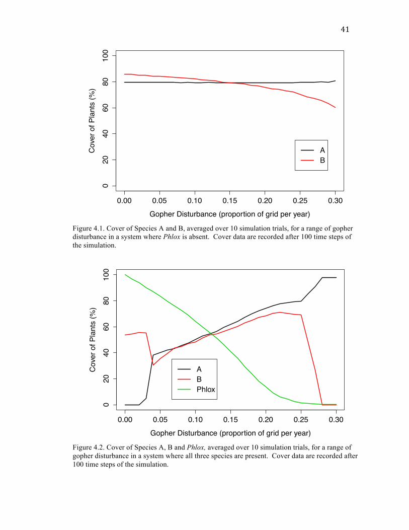
41

Figure 4.1. Cover of Species A and B, averaged over 10 simulation trials, for a range of gopher disturbance in a system where Phlox is absent. Cover data are recorded after 100 time steps of the simulation.

Figure 4.2. Cover of Species A, B and Phlox, averaged over 10 simulation trials, for a range of gopher disturbance in a system where all three species are present. Cover data are recorded after 100 time steps of the simulation.

0.00 0.05 0.10 0.15 0.20 0.25 0.30

020

4060

8010

0

Gopher Disturbance (proportion of grid per year)

Cov

er o

f Pla

nts

(%)

AB

0.00 0.05 0.10 0.15 0.20 0.25 0.30

020

4060

8010

0

Gopher Disturbance (proportion of grid per year)

Cov

er o

f Pla

nts

(%)

ABPhlox

42

Model findings

Using parameters constructed from a basic set of assumptions, I was able to show

that it could be possible for the presence of a dominant species such as Phlox to reverse

the nature of the relationship between disturbance and graminoids. With reproductive

and competitive parameters for Species A and B held constant, I found that when Phlox

was not present Species B declined with increasing disturbance, but once Phlox was

added to the system Species B increased over a certain range of disturbance (roughly 0.04

to 0.22).

Phlox shows a monotonic negative relationship with disturbance. Species A was

constant in abundance across the range of disturbance tested when only Species A and B

were present, and once Phlox was added Species A showed a more pronounced positive

relationship with disturbance. At the outer limits of the range of disturbance tested in the

three-species case, the hypothetical system is less stable and only one or two species can

persist (presenting, consequently, an illustration of the Intermediate Disturbance

Hypothesis). Species A is absent for very low rates of disturbance (up to about G = 0.04,

at which point the abundance of Species B drops because Species A is also present and

competing for space). For roughly G > 0.27, both Species B and Phlox disappear or

nearly disappear and Species A dominates.

43

Chapter 5

Discussion

This study sought to investigate the effects of gopher disturbance on plant

community structure in montane meadows at Bunchgrass Ridge, Oregon. Two primary

goals were (1) to explore relationships at larger spatial scales than previously studied in

this system (Jones et al. 2008), and (2) to assess the contributions of the two main forms

of disturbance—mounds and castings—to these relationships. The effects of castings

were of particular interest because relationships between castings and vegetation have not

been studied before. As a way of explaining unexpected variation in the relationships

between disturbance and vegetation among individual plots, I also created a simulation

model that showed how the presence of a particularly competitive species could alter

these relationships. In this chapter I will interpret my findings, discuss their broader

implications, and suggest additional studies that could inform our understanding of the

role of gopher disturbance in the community structure of montane meadows.

Castings are a considerable form of disturbance

One objective of this study was to explore the contributions of mounds and

castings to the broader effects of disturbance on plant communities. Gopher castings are

a striking feature of higher-altitude meadows, where extensive winter tunneling can occur

in a deep, long-lasting snow pack. The effects of castings on plant communities have so

far been ignored in the literature, perhaps because they are not present in the lowland

communities where most studies of gopher-plant interactions have been conducted, or

44

because they are a more ephemeral form of disturbance and are less conspicuous than

mounds once meadow vegetation matures. The only mentions of castings I have found

do not explore their potential effects on vegetation (Reichman 2007, Knight 2009). Upon

observing the ubiquity of castings at Bunchgrass, however, I hypothesized that the

castings would have an impact on plants.

I found that plant cover was negatively correlated with cover of mounds and

cover of castings. This finding indicates that castings are a significant form of gopher

disturbance that impacts plants and should not be ignored. Castings are abundant at

Bunchgrass, covering about 10% of the ground surface on average and making up

roughly one-third to one-half of all gopher disturbance present in each meadow sampled.

The remainder of gopher disturbance sampled consisted mainly of old mounds, which

had been created at least one year previously. The two types of disturbance are different

in several notable ways, which I will explore further as these differences relate the

interpretation of my findings. Mounds are deeper and longer-lasting, and the soil

composition of mounds and castings appears to differ. The mounds and castings sampled

also differed in age; old mounds had been created in the previous growing season or

earlier (in effect, integrating over multiple years of past disturbance), whereas castings

were created more recently over the course of the winter.

Fresh mounds that had formed in the current growing season were extremely

infrequent in the plots, even during vegetation sampling in July and early August. I

observed a greater abundance of fresh mounds beginning to appear in the meadows in

mid-August, just before I concluded vegetation sampling. Given these observations, it

seemed likely that most mound-forming activity occurs in late summer to fall. This

45

agrees with reports from lowland prairies in Western Washington, which share the same

pattern of summer drought common in higher-elevation grasslands in the Pacific

Northwest, that Thomomys mazama is most active when fall rains begin (G. Olson, pers.

comm.). In July 2004, however, Jones et al. (2008) found that 33% of mounds

intersected by line transects across three meadows at Bunchgrass were fresh mounds.

Snow melt occurred unusually late in the summer when I conducted my study, with snow

pack persisting into mid-June in some meadows. Perhaps these conditions affected the

level of gopher activity in early summer because the period of time between snow melt

and summer drought was shortened. The plant cover I observed could easily have

differed had there been more fresh mounds present, but my findings are still useful for

assessing the effects of castings and older mounds.

Spatial correlation patterns show clumping at small scales

Cover of mounds and castings were correlated with each other within quadrats (20

cm x 20 cm), but uncorrelated on the scale of transects (5 m x 20 cm). This correlation at

small spatial scales may be due to gophers tunneling around or through mounds as a

means of structural support under the snow. Elsewhere in the meadows I observed

castings built up next to fallen logs and the bases of trees, possibly for the same reason.

For each form of disturbance – as well as for total plant, forb, and graminoid

cover – I also found high spatial autocorrelation at distances < 1 m. Given that mounds

are typically much less than 1 m in diameter (Jones et al. 2008), this finding suggests that

mounds are clustered spatially. The finding of similar autocorrelation patterns among

cover of disturbance and plant variables could mean that the spatial structure of gopher

46

disturbance determines the spatial patterns of plant abundance, or vice versa. This could

also be a coincidence, however, as there are plausible reasons intrinsic to disturbance and

plants for why each would show autocorrelation at that scale: mounds could be correlated

within 1 m because multiple mounds are created around the same gopher hole; plant

cover could be correlated within 1 m because plants spread clonally or have limited seed

dispersal distances. Regardless, my findings of spatial autocorrelation for both forms of

disturbance add to the existing literature on similarly clustered patterns found in other

grassland systems (Thomson et al. 1996, Klaas et al. 2000, Wolfe-Bellin & Moloney

2000, Overton & Levin 2003).

Disturbance effects on forbs and graminoids

As expected, plant cover declined with increasing total disturbance. The

relationships between total disturbance and forb and graminoid cover, however, appeared

inconsistent across plots, with no significant overall relationship found for either forbs or

graminoids or the ratio between the two. These non-significant overall relationships may

be related to a high degree of variability among plots in the slopes that describe the

relationships. Random slope coefficients suggested that graminoids did not decline with

disturbance in Plot 3, in contrast to apparent declines in the other three plots, and that

forbs (whether or not Phlox was included as a forb), declined with disturbance in some

plots but increased in others. The ratio of forb to graminoid cover, consequently, was

also not consistent across plots.

Many other studies (including the previous study at this site) have found that

gopher disturbance benefits forbs relative to graminoids (Mielke 1977, Foster &

47

Stubbendieck 1980, Martinsen et al. 1990, Sherrod et al. 2005, Jones et al. 2008), so I

had expected to find similar relationships in my plots, particularly for the forb/graminoid

ratio. All previous studies of gopher disturbance, however, have focused only on mounds

(ignoring castings), so it is thus possible that lack of consistency with the literature in my

analyses simply reflects differences in the definitions of “disturbance.” Breaking down

total disturbance into the different types of disturbance present, we see that the

relationship between mounds and relative abundances of growth forms is consistent with

previous studies. Graminoid cover was negatively correlated with mound cover and

consequently the forb/graminoid ratio increased with mound cover. Castings,

meanwhile, had no significant effect on either graminoids or the forb/graminoid ratio.

These results suggest that the neutral or variable effect of the castings on graminoids

masks the strong negative relationship between mounds and graminoids when both forms

of disturbance are summed.

There is still the question of what might explain non-significant relationships

between castings and the relative abundance of different growth forms. Castings did

have a strong negative relationship with total plant cover, so the answer is not that

castings were not affecting plants at all, but that relationships with individual growth

forms were not consistent. The differing slopes predicted for graminoids vs. castings

across the four plots mirrored the variability in slopes found for graminoids vs. total

disturbance (negative in Plots 1, 2, and 4, and positive in Plot 3), and likewise for the

suggested relationships between the forb/graminoid ratio and castings (positive in Plots 1,

2, and 4, and negative in Plot 3). It is also worth noting that neither mounds nor castings

affected forb cover significantly, which is also likely due to variability among plots,

48

given that the predicted slopes are positive for some plots and negative for others. We

can examine these findings in two ways: first, why might castings and mounds have

different effects on vegetation, and second, why might growth form relationships with

disturbance vary among plots?

A likely answer to the first question is that mounds and castings differ in size and

longevity, which could explain some of the differences in how the two forms of

disturbance affect vegetation. Mounds tend to be larger than castings in diameter and

height; mounds are typically round or oblong and range from 20-50 cm in diameter and

5-25 cm in height (Reichman 2007) while castings are long and skinny, typically 5-10 cm

across and no more than a few cm in height. While castings are assimilated into the

meadow matrix relatively quickly, most likely within a single growing season (Halpern,

pers. comm.), mounds can last for years before the gradual process of weathering and re-

vegetation obscures them (Reichman 2007). In combination, the greater size and

longevity of mounds might present more substantial barriers to re-emergence from burial

for graminoids, if vegetative recovery is an important factor in differentiating between

forb and graminoid responses. Sherrod et al. (2005) hypothesized that the relative

success of forbs in colonizing mounds in alpine tundra at Niwot Ridge could be attributed

to their greater belowground carbohydrate stores, which facilitated emergence from

burial.

My own observations of excavated root systems of plants growing on mounds

suggest that many of the forb species in these meadows appear capable of recovering

from burial. I have found examples of Iris chrysophylla, Lupinus latifolius, Cirsium

callilepis, Hieracium gracile, Erigeron aliceae, and Comandra umbellata where old root

49

systems could be found 5-10 cm below the surface of the mound (at the former ground

surface) and plants had sent up emergent shoots and developed new clusters of roots near

the new soil surface. The only graminoid that I found exhibiting this trait, by contrast,

was the highly rhizomatous sedge Carex pensylvanica, a dominant species in these

meadows. Other graminoid species – Bromus carinatus, Danthonia intermedia, and

Festuca idahoensis – that I excavated from mounds had shallow fibrous root systems and

appeared to have colonized the mounds by seed. On mounds, the ability of forbs to

emerge from burial and persist in a location where they are already established could give

them an advantage. Castings, however, may be shallow enough that even graminoids

buried by castings can survive, and as a result the ratio of forbs to graminoids may not be

affected by castings even if plant cover is reduced.

Another key distinction is that the mounds and castings analyzed in this study

represent disturbances of different ages. Because fresh mounds were virtually absent, I

was comparing old mounds, which had been present since at least the previous growing

season and possibly multiple years previous, and recent castings, which had appeared at

the beginning of the current growing season. Considering the age differences of the two

types of disturbance, it is not surprising that their effects differ. Old mounds and castings

represent different moments in the process of succession. As fresh sites of disturbance,

the main effect of recent castings may be simply to reduce plant cover indiscriminately.

Old mounds are at a slightly later point in the process of re-vegetation, where plants have

had a chance to respond but differences between growth forms in their early success on

mounds are still apparent. Combining this observation with the differences in size and

longevity of disturbance types noted above, we can hypothesize that castings may

50

transition quickly from a state with no plant cover to a state at which all plant species

have had a chance to re-vegetate castings, with the result that castings do not modify

species composition as appreciably as mounds do.

The second question raised by my findings is why the relationships between

different growth forms and disturbance might vary across plots or meadows. One

plausible explanation is that growth form categories do not capture all of the relevant

variation in plant traits that determine responses to disturbance. The species abundance

data in Table 3.2 illustrate that while plots shared many species in common, no two plots

contained exactly the same collection of species in the same abundances. Within each

growth form, there is still substantial variation in many plant traits that may affect

susceptibility to or resistance to effects of burial: large forbs that stand taller than their

neighbors (Lupinus latifolius, Hieracium gracile) and small forbs that grow underneath

other plants (Arenaria macrophylla, Viola nuttallii); non-rhizomatous bunchgrasses

(Festuca idahoensis, Stipa occidentalis) and highly rhizomatous sedges (Carex

pensylvanica). Species within a growth form could vary tremendously in growth rates,

modes of reproduction, and strength of competition with other species, so we cannot

assume that all species within a growth form will show the same relationship to

disturbance. The overall relationships between disturbance and total cover of growth

forms, therefore, might vary depending on the particular combination and relative

abundance of species present in each meadow.

51

Modeling results

The simulation model presented in Chapter 4 offers another possible explanation

for variability in patterns of graminoid response to disturbance. Motivated by my

observations that Phlox appeared particularly dominant in Plot 3, where the data also

suggested a neutral or positive relationship between disturbance and graminoids, the

model shows that the prevalence of a highly competitive species such as Phlox can

potentially alter the nature of the relationship between disturbance and other plant

species. The graminoid-like species in the model, Species B, declined with higher yearly

rates of disturbance when Phlox was absent, but benefited from higher rates of

disturbance when Phlox was present. This shift occurs about because Phlox is a poor

colonizer after disturbance, and a better competitor than Species B if not disturbed. With

only Species A and B present, Species B was the best long-term competitor in the system,

so it benefited from lower rates of disturbance. When Phlox was present, however, the

Phlox dominated the meadow unless gopher disturbance created openings; under these

conditions, the abundance of Species B was largely determined by how many gaps were

opened in the Phlox matrix, so Species B showed a general trend of increasing with

disturbance.

The model simplifies many aspects of this meadow ecosystem, and without

information on actual growth and reproduction rates of the species involved it is not

possible to demonstrate that it represents the true interactions that structure these

communities. It does illustrate, however, that disturbance effects may depend on the

species composition of each meadow and where each species falls on the hypothetical

52

spectrum from “good colonizer” to “good competitor”. A highly competitive dominant

species has the potential to alter the relationships between other species and disturbance.

Effects of disturbance on diversity

In addition to effects on growth-form abundance, I was also interested in the

relationship between disturbance and species diversity and whether the Intermediate

Disturbance Hypothesis could apply to these meadows. I found a positive relationship

between species richness at the scale of transects and total cover of disturbance. Spatial

heterogeneity (variation in species composition), which can be considered another aspect

of diversity, also showed a positive relationship with total disturbance. Evenness

(calculated as a modified Hill ratio) was uncorrelated with total disturbance, which

agreed with the previous finding in this system of no difference in evenness between

mounds and undisturbed meadow (Jones et al. 2008). Examination of the scatterplots of

evenness index vs. disturbance by plot, as well as the finding that a random slope term

did not improve the fit of the model, suggested that there was no relationship in any plot

(rather than differing relationships among plots as with some of the other response

variables).

It is unclear whether my richness results are consistent with the Intermediate

Disturbance Hypothesis. In this study, cover of disturbance reflects both frequency and

intensity of disturbance; because mounds can last multiple years, a high cover of

disturbance could result from gopher activity that is either more frequent, or more intense

in spatial extent within a single year. The relationship I found between richness and

disturbance was best modeled with a positive linear relationship, whereas the IDH

53

predicts a humped relationship that peaks at intermediate levels of disturbance (Connell

1978). However, since none of the transects exceeded 60% total disturbance, it could be

argued that I did not sample a broad enough range of disturbance to be able to observe a

peak or decline in richness associated with greater cover of disturbance. Indeed, along a

spectrum from 0-100% disturbance, 60% could be considered approximately

intermediate. If a transect were 100% disturbed, one can imagine that plant cover would

be so minimal that a high species richness would be unlikely, so it is plausible that

richness would indeed decline for cover of disturbance greater than the maximum

sampled in this study.

Comparing my findings on diversity-disturbance relationships to those of Jones et

al. (2008) requires a consideration of scaling effects. Jones et al. (2008) found greater

species richness in small quadrats in undisturbed vegetation than on mounds (young or

old), from which they inferred a pattern of gradual accumulation of species as mounds

age. If we simplify this result to one of disturbed vs. undisturbed patches on a small scale,

disturbed patches contain fewer species than undisturbed patches, which suggests a

negative relationship between disturbance and species richness.

In my study, however, I found a positive relationship between disturbance and

species richness at the transect scale. Does this finding contradict Jones et al. (2008)?

Not necessarily, if we consider the role of spatial heterogeneity, which Auerbach &

Shmida (1987) argue becomes a more important factor in determining richness as the

spatial scale of inquiry begins to exceed the size of any individual organism. Jones et al.

(2008) found that species composition differed more between quadrats on mounds than

between quadrats in undisturbed vegetation, and based on this result hypothesized that on

54

a larger scale gopher disturbance would increase spatial heterogeneity in meadows. My

finding that the transect-scale compositional heterogeneity increased with disturbance

supports this hypothesis.

We can think of a transect as consisting of an aggregation of many small

disturbed and undisturbed patches. An individual patch of disturbed meadow might

contain fewer species than its undisturbed neighbor. Any two disturbed patches,

however, are more likely to contain unique species (Jones et al. 2008). This implies that

a greater amount of disturbance increases the potential for rarer species to establish,

leading to greater heterogeneity of composition as well as a richer assemblage of species

at the transect scale. In this way, it is possible to reconcile the small-scale findings of

Jones et al. (2008) with my larger-scale findings. My findings reinforce the notion that

diversity-disturbance relationships seen in nature are highly dependent on the spatial

scale of inquiry (Chaneton & Facelli 1991).

Heterogeneity in species composition was positively correlated with mounds,

while the effect of castings was insignificant. This result may have emerged from the

greater impact mounds seem to have on the relative abundance of major growth forms,

which would help make quadrats containing mounds more compositionally different from

other quadrats in a transect. Species richness, however, was positively correlated with

cover of castings, while only marginally significant in its relationship with mounds. This

finding is more difficult to explain. One possible justification is that the soil composing

mounds and castings may have been excavated from different depths. As noted in the

description of the methods, castings contained fewer small stones and more bits of

organic matter such as small pieces of grass. This seems to indicate that much of the soil

55

that makes up castings comes from tunnels excavated at the interface between the snow

and the ground surface. Thus castings might be more likely to contain viable plant parts

or seeds that have been transported by the gophers from elsewhere in the meadow,

resulting in an enrichment of the number of species present in a transect. Given that the

soil seed bank is relatively poor in these meadows, however (Lang & Halpern 2007), the

possibility of castings containing numerous relocated propagules is fairly unlikely. The

near-significance of the effect of mounds on richness suggests that in this case, the

physical differences between mounds and casts are probably not particularly important,

and with a greater sample size we might find that both forms of disturbance contribute

significantly to an increase in richness.

Future directions

Long-term and experimental studies

Montane meadows are dynamic systems. There is only so much we can learn,

consequently, from the static snapshot of meadow conditions gained in this observational

study, or even from the chronosequence approach used by Jones et al. (2008), which used

a comparison of mounds of different ages as a proxy for observation through time. Long-

term studies of gopher impacts in other systems have proven very informative,

particularly in illustrating how gopher disturbance and plant community dynamics can

vary from year to year and interact with fluctuations in climate (Hobbs & Mooney 1991,

Wolfe-Bellin & Moloney 2000, Forbis et al. 2004). Further study at Bunchgrass Ridge

or similar study sites should allow for the possibility of observing changes through time,

ideally over multiple years (my transects are still marked, so there is in fact an existing

56

opportunity for re-sampling gopher disturbance and vegetation at Bunchgrass). In

particular, observation of succession on mounds and castings over time would allow for

clearer comparisons between the two types of disturbance, avoiding the confounding

effects inherent in this study’s comparisons of recently created castings to mounds at

least a year old.

Another limitation of the observational approach used in this study is that it

makes causal inference difficult, especially given the potential for feedback mechanisms

between gophers and plants. I treated gopher disturbance as the explanatory variable and

plant community characteristics as the response variables, but it is conceivable that the

distributions of plants could also determine where, and to what extent, the gophers create

disturbance. Indeed, multiple studies have considered how the distribution of gopher

disturbance can be seen as a non-random response to the distribution of plants, whether

because gophers preferentially dig their burrows in areas populated by the plants they

prefer to eat (Seabloom & Reichman 2001), or because gophers avoid digging through

the ground underneath plants with more obstructive root systems (Watts 2010). By

simply observing the patterns of gopher disturbance and associated plant cover, it is

difficult to say for sure how much the gophers are influencing the plants or vice versa.

Fortunately, there is potential for experimental manipulations, which can help

unravel cause-and-effect relationships. Studies in other systems have investigated factors

driving gopher preferences in digging location by monitoring gopher response to

fertilization treatments (Tilman 1983) and by establishing monocultures of common

plants to compare which species seem to invite greater gopher activity (Eviner & Chapin

2003). Conversely, to isolate gopher disturbance as the cause and plant response as the

57

effect, Sherrod et al. (2005) created artificial gopher mounds using soil from fresh

mounds, which allowed them to measure pre-treatment vegetation and directly observe

which species were most successful at recovering from burial over the course of a year.

Such an approach could potentially be applied at Bunchgrass Ridge as well. This was, in

fact, my original research plan (Case 2011), but time constraints and a lack of fresh

mounds early in the summer made it infeasible. An experiment that involved creating

gopher mounds and measuring the vegetation on them a year later, or even over the

course of multiple years, could give us a more precise understanding of the path of

succession on mounds.

Studies of plant regenerative traits

As a potential explanation for the variation in growth-form response among plots,

I suggested that individual species within each growth form could vary greatly in the

traits that determine their disturbance responses. Consequently, a more detailed

understanding of key differences in regenerative and other functional traits could provide

insight into what drives patterns of plant community response to gopher disturbance.

One important avenue of exploration would be a more systematic study of the

belowground characteristics of plants via excavations of plants experiencing different

amounts of natural disturbance (as suggested in Case 2011). Such excavation studies

have been conducted in forest environments of the Pacific Northwest, illustrating the

ways in which belowground characteristics of understory species are important to

patterns of successional change (Antos & Halpern 1997, Lezberg et al. 1999). An

artificial mound experiment, as outlined above, could also allow for focused monitoring

58

and excavation of particular species to determine patterns and relative rates of lateral

growth and emergence from burial.

More realistic modeling approaches

The simulation model I designed as part of this study was an initial, relatively

simple attempt to better understand this system better through modeling. My model was

conceived of as a qualitative test of a hypothesis using parameters invented to match the

starting assumptions, which works to show that a proposed relationship between Phlox,

graminoids, and disturbance is theoretically possible. This model could be modified to

better reflect the processes that determine survival and reproduction following

disturbance. The characterization of reproduction by Species A and B as a random

dispersal of propagules over the grid that are guaranteed to germinate and survive is a

simplification that was used to streamline the process of finding reasonable parameters

for A and B. Given the prevalence of vegetative reproduction in this system, a major step

in improving this model would be to modify the mechanism of reproduction of all species

involved, not just Phlox, to better reflect vegetative processes. In addition, most models

of gopher-plant interactions have made use of parameters drawn directly or indirectly

from empirical studies, allowing more confident conclusions about how their results

apply to the real world (Hobbs & Hobbs 1987, Moloney & Levin 1996, Wu & Levin

1994). My model should be seen as a starting template, into which actual parameters for

growth, competition and reproduction could be inserted to produce results that are more

quantitatively applicable.

59

Conclusions

My results show that mounds and castings both impact plants. Future studies of

how gopher disturbance affects plants should take care to consider the role of castings,

which has been ignored until now. Comparisons between mound and casting

relationships with plant response variables, and my finding of inconsistency in some of

these relationships among plots, illustrate that interactions between disturbance and

community composition are variable and complex. The physical and temporal

distinctions between mounds and castings as well as differences in species composition

among meadows can all play a role in determining the patterns that emerge. As my

simulation model demonstrates, it is conceivable for the presence or absence of a highly

competitive species to drastically change the nature of disturbance-vegetation

relationships.

My study also illustrates important considerations of spatial structure in gopher

disturbance. I found a high degree of clumping in gopher disturbance and plant cover at

small spatial scales, which leads to a spatially heterogeneous landscape overall. Hence

the spatial scale at which we observe patterns of diversity and heterogeneity matters

greatly, as illustrated by the contrast between my findings and those of Jones et al. (2008)

regarding the relationship between disturbance and species richness.

The montane meadows at Bunchgrass Ridge, like many natural systems, are

driven by non-equilibrium dynamics. This study helps show how persistent disturbance

can play a critical role in shaping the structure of plant communities.

60

Appendix A

Brief Overview of Mixed Effects Models

A mixed effects model is a statistical model that combines both fixed and random

effects. Mixed effects models are useful for avoiding pseudoreplication in analyzing

clustered data, which is what I had in this study with multiple transects sampled per plot.

The fixed component accounts for the overall relationship between the explanatory

variable(s) of interest and the response variable, while the random component accounts

for variation among individuals or plots. A typical formulation of a linear mixed effects

model is thus:

Y! =  X!×𝛽  +    Z!×b! +  𝜀!

Here, Y! is the response variable, X!×𝛽 is the fixed component (the parameter 𝛽 has no

index because it applies across all individuals), Z!×b! is the random component, and 𝜀!  is

the random error term. Like 𝜀!, the term b! is assumed to be an i.i.d. normally distributed

random variable; we are assuming, essentially, that individual variation about the central

tendency of the population is normally distributed with a certain variance (Zuur et al.

2009).

Linear mixed effects models can be constructed with different random effects

structures: random intercept only, or random intercept and slope. In a random intercept

model, the intercept is allowed to vary by individual, but there is no variation in slope

about the overall population slope 𝛽. In a random intercept and slope model, both

intercepts and slopes are allowed to vary according to random effects (Zuur et al. 2009).

In this study I used random intercept and slope models unless a likelihood-ratio test

61

showed that the random intercept only model presented an equally good or better fit to

the data.

The question of how best to calculate a p-value for the significance of a fixed

effects term in a mixed effects model is debated. Douglas Bates, creator of the lme4

package in R, declines to include an output of p-values in the lmer() function (the

function I used for my analysis) because he argues that the calculation of denominator

degrees of freedom used by mixed effects model functions in other statistical programs is

suspect (Bates 2006). Bates recommends using Markov Chain Monte Carlo sampling to

estimate a p-value for fixed effects; the function designed to do this, however, has not yet

been developed to work with random intercept and slope models with correlated random

effects, so it was not applicable to many of my analyses. As an alternative I used the

pamer.fnc() function from the LMERConvenienceFunctions package (Tremblay 2011),

which deals with the issue of uncertain degrees of freedom by calculating a plausible

upper and lower bound on degrees of freedom and finding p-values accordingly.

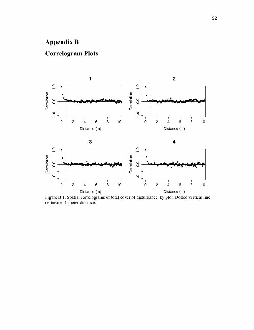
62

Appendix B

Correlogram Plots

Figure B.1. Spatial correlograms of total cover of disturbance, by plot. Dotted vertical line delineates 1-meter distance.

●

●

●●●●●●●●●●●●●●●●●●

●●●●●●●●●●●●●

●●●

●●●●●●●●●●●

●●●●●●●●●●●

●●●●●●●●●●●●●●●●

●●●●●●●●●●●●

●●●●●●●●●●●●●

●●●●●●●●●●

●●●●●●●●●

●●●●●●●●●

●●●●●●●●

●●●●●●●

●●●●●●●●●●●●●●

●●●●●●●●●●●●●

●

●

●●●●●●●●●●●●●

●

●●●●●●●●●●●

●●

●●●●●●●

●●●●

●

●

●●●●●●●

●

●

●●

●●●

●●●

●●

●●

●

●●●●●●

●●●

●

●●●●●●●

●

●

0 2 4 6 8 10

−1.0

0.0

1.0

1

Distance (m)

Cor

rela

tion

●

●

●●●●●●●●●●

●●●●●●●●●●●●●●●●●●●●●●●●●

●●●●●●●●●●●●

●●

●●●●●●●●●●●●●●●●●●●●●

●●●●●●●●●●

●●●●●●●●●●●

●●●●●●

●●●●●●●●●●●●●●

●●●●●●●●

●●●●●●●●●●●●●●●●●●●

●●

●●●●●●●●●●●●●

0 2 4 6 8 10

−1.0

0.0

1.0

2

Distance (m)C

orre

latio

n

●

●

●●●●●●

●●●●

●●●●●●●●●●●●●●●●●●●●●●●●●

●●●●●●●●●●●●●

●

●●●

●●●●●●●●●●●●●●

●●●●●●●●●●

●●●●●●●●●●●●●●●●

●●●●●●●●●●●●●

●●●●●●●●●●●●●●●●●●●●●●●●●●●●●●●●●●●●●●●●●

●●●●●

●●●●

●●●●●●●●●●

●●●

●●●●●●●●●●●●●●●●

●●●●●●●●

●●

●

●

●●●●●●●●●●●

●●

●●

●

●

●●

●●●●

● ●●●

●●●●●

●

●

●

●●

●●●●●

●●

●

●●●

●

●

●●

●

●

0 2 4 6 8 10

−1.0

0.0

1.0

3

Distance (m)

Cor

rela

tion

●

●

●●●●●●●●●●

●●●●●●

●●●●●●

●●●●●●●●●●

●●●●●●●●

●●●●●●●●●●●

●

●●●●●●●●●●●●●●

●

●●●●●●●●●●●

●●●●●●●●●●●●●●●●●●●

●●●●●●●●●●●●●

●

●●●●●●●●●●●●●

●

●●●●●●●●●

●●●●●●

●●●●●●●●●●●●●

0 2 4 6 8 10

−1.0

0.0

1.0

4

Distance (m)

Cor

rela

tion

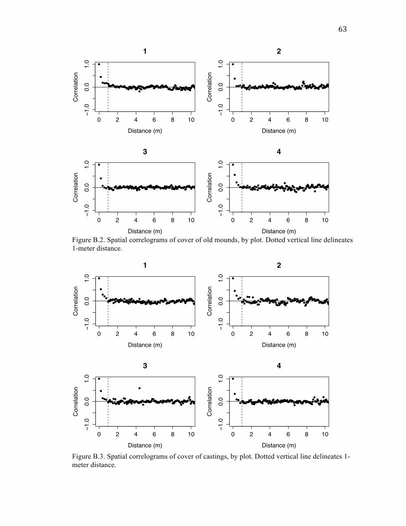
63

Figure B.2. Spatial correlograms of cover of old mounds, by plot. Dotted vertical line delineates 1-meter distance.

Figure B.3. Spatial correlograms of cover of castings, by plot. Dotted vertical line delineates 1-meter distance.

●

●

●●●●●●●●●

●●●●●●●●●●●●●●●●●●●●●●

●●●●●●●●●●●

●●●●●●

●●●●●●●●●●●

●●●●●●●●●●●

●●●●●●●●●●●

●●●●●●●●●●●●●●●●●●

●●●●●●●●●●

●●●●●●●●●●●●●●●●

●●●●●●●●●

●●●●●●●●●●●

●●●●●●●●●

●●●●●●●●●●●●●●●

●●●●●●●●●

●●●

●

●●●●●●●●●●●●

●

●

●●●●●●●

●

●

●

●

●

●

●●●●●●●

●

●

●

●

●●●

●●●●●

●

●

●

●●●●●●●●

●

●●●●

●

●

●●●●

0 2 4 6 8 10

−1.0

0.0

1.0

1

Distance (m)

Cor

rela

tion

●

●

●●●●●●●●●●●

●●

●●●●●●●●

●●●●●●●●●

●●●●●●●●●●●●●

●●●●●

●

●●

●

●●●●●●●●●●●●●●

●●●●●●●●●●●●●●●●●

●●●●●●●●●●●●●●●●●●●●●●●●●●●●●●●●●●

●●●●●

●●●●●●●●●●●●●●●●●●

●●●●●●●●●●●

●●

0 2 4 6 8 10

−1.0

0.0

1.0

2

Distance (m)

Cor

rela

tion

●

●

●●●

●●●●●●●●

●●●●●●●●●●●●

●●●●●●●●●●●●●

●●●●●●●●●●●●●●●●●●●●●●●●

●●●●●●●●●●●●

●●●●●●●●●●●●●●●●●●●●●●

●●

●●●●●●●●●●●●●●●●●●●●●

●●●●●●●●●●●

●●●●●●●●●●●●●●●●

●●●●●●●●●●●

●●●●●●●●●●●●

●●●●●

●●●●●●●●●●●●●●●●●●●●●●●●●●●●●●●●●●●●●●

●●●●●●●●●● ●

●●●●●●●●●● ●●

●●●●●●●●

●

●●

●●●●●●

0 2 4 6 8 10

−1.0

0.0

1.0

3

Distance (m)

Cor

rela

tion

●

●

●●●●●●

●●●●●●●●●●●●●●●●●●

●●●●●

●●●●●●●●●●●●●●●●●●●●●●●●●

●●●●●●●

●●●●●

●

●●●

●●●●●●●●

●●●●●

●●●●●●●●●●

●●●●●●●●●●●●●●●●●

●

●●●●●●●●●●●●

●●●●●●●●●●●●●●

●●●●●●●●●●●●●●●●

0 2 4 6 8 10−1

.00.

01.

0

4

Distance (m)

Cor

rela

tion

●

●

●●●●●●●●●●

●●●●●●●●●●●●●●

●●●●●●●●●●●●●●●●●●●●

●●●●●

●●●●●●●●●●●●●●●●●●●●●●●●●●●●

●●●●●●●●●

●●●●●●●●

●●●●●●●●●●●●●●●●●●

●●●●●●●●●●●●

●●●●●●●●●●●●●●●●●●●●●●●●●●●●●●●

●●●●●●●●●●●●

●

●

●●●●●●●●●●●●●●

●●●●●●●●●●●●●●●●●●●●●●●●●

●●●●●●●●●●●● ●●●●●●●●●●● ●●●●●●●●●●

●●●●●●●●●

0 2 4 6 8 10

−1.0

0.0

1.0

1

Distance (m)

Cor

rela

tion

●

●

●●●

●●●●

●●●

●

●

●

●●●●

●

●●●●●●

●

●●●●●●●●●●●

●●●●●●●●●●●●●

●●●●●

●

●●●●●●●●●●●●●●●

●●●●●●●●●●

●●●●●●●●●●●●●●●●●●●●●●●●●●●●●●●●●●●●●

●●●●●●●●●●●●●●●●●●●●●●●●

●●●●

●●●●●●●●

0 2 4 6 8 10

−1.0

0.0

1.0

2

Distance (m)

Cor

rela

tion

●

●

●●●●●●●●●●

●

●

●

●●●●●●●●●●●

●

●

●●●●●●●●●●●●●●●●●

●●●●●

●

●●●●●

●●●●●

●●●●●●●●●●●●●●●●●●●●●

●●●●●●●●●●

●●●●●●●●●●●●●●●●●●●●

●●●●●●●●●●●●

●●●

●●●●●●●●●●●●●●●●●●●●●●

●●●●●●●●

●●●●●●●●●●●●

●●●●●●

●

●●●●●●

●

●

●

●●●●●●●

●●

●●●

●●●

●

●●●●●●

●●

●

●●●

●

●

●●

●●

●

●

● ●

●

●

●

●

●●

●

●

●

●

●

●

●●●

●

●

●

●

●

●

●

●

●

●

●●

●●

0 2 4 6 8 10

−1.0

0.0

1.0

3

Distance (m)

Cor

rela

tion

●

●

●●●●●●●●●●●●

●●●●●●●●●●●

●●●●●●●●

●●●●●●●●●●●●●●●●●●●●●●●●●●●●●

●●●●●●●●●●●●●●

●●●●●●●●●●●●●●●●●●●

●●●●●●●●●●●●●●●●●

●●●●●●●●●●●●●

●●●●●●●●●●●

●●●●●●●●●●●●●●●●●

●●

0 2 4 6 8 10

−1.0

0.0

1.0

4

Distance (m)

Cor

rela

tion

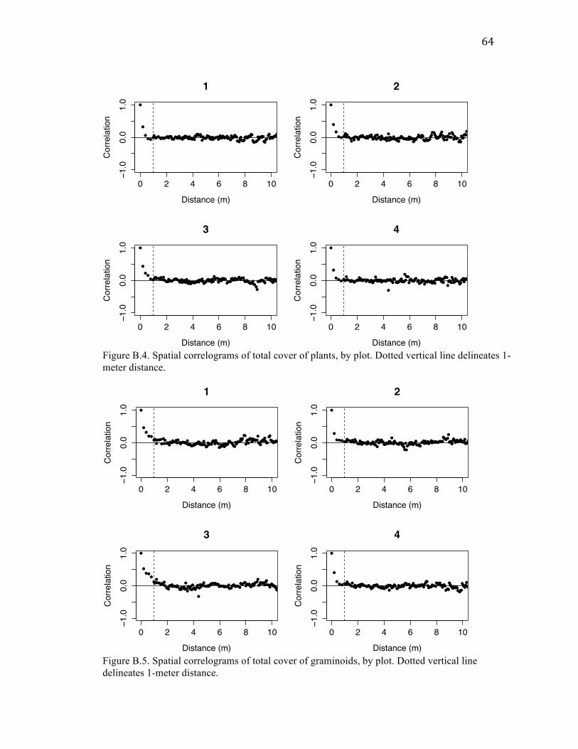
64

Figure B.4. Spatial correlograms of total cover of plants, by plot. Dotted vertical line delineates 1-meter distance.

Figure B.5. Spatial correlograms of total cover of graminoids, by plot. Dotted vertical line delineates 1-meter distance.

●

●

●●●●

●●●●●●●●●●●●●●

●●●●●●●●●●●●●●●

●●●●●●●●●●●●●●●●●●●●

●●●●●

●●●●●●●●●●●

●●●●●●●●●●●●●●

●●●●●●●●●●●●●●

●●●●●●●●●

●●●●●●●●●●●●●●●●●●●●●●●

●●●●●●●●●●●●●●●●●●●●●●●

●●●

●●●●●●

●●●

●●●

●●●●●●●

●●●●

●●●●●●●●●●●●

●

●●●●●●●●●●●

●●

●

●●

●

●

●●●●●●

●

●

●●

●

●●●●

●

●

●

●●●

●

●●●

●●

●●●

●●

●●●●

●

●

●●

●

0 2 4 6 8 10

−1.0

0.0

1.0

1

Distance (m)

Cor

rela

tion

●

●

●●●●

●●●●●●●●●●●●●●

●●●●●●●●●●●●●●

●●●●●●●●●●●●●●●

●●

●●●●●●●●●●●●●●●●●●●●●

●●●●●●●●●●●●●●●●●●●●●●

●●●●●●●●●●

●●●●●●●●●●●●●●●

●●●●●

●●●

●●●●●●●●●●●●●●●

●●●●●●●●●●

●●●

0 2 4 6 8 10

−1.0

0.0

1.0

2

Distance (m)

Cor

rela

tion

●

●

●●●●●

●●●●●●●●●●●●

●●●●●●●●●●●●

●●●●●●●●●●●●●●●●●●●

●●●●●●●●●●●●●●●●

●●

●●●●●●●●●●●●●

●●●●●●●●●●●●

●●●●●●●●●●●●●●●●●●●●

●●●●●●●●●●●●●●●●●●

●●●●●●●●●●●●●●●

●●●●●●●●●●

●●●●●●●●

●●●●

●●●

●●●●●●●●●●

●●●

●

●●●●●

●

●●●

●●●●●●●●

●●●●●●●●●

●●●●

●

●

●●●●● ●

●●●●●●●●

●●

●●●

●●

●

●

●

●

● ●

●

●

●●●

●

●

●

0 2 4 6 8 10

−1.0

0.0

1.0

3

Distance (m)

Cor

rela

tion

●

●

●●●●●●●●●●●●●●●

●●●●●●●●●●●●●●●●●

●●●●●●●●●●●●●●●

●

●

●●●●●●●●●●●●

●●●●●

●

●●●

●●●●●●●

●●●●●●●●●●●●●●●●●●●●

●●●●●●●●●●●●●

●●●●●

●●●●●●●●●●●●●●●●●●●●●●●●

●●●●●●●●●●●●●●

0 2 4 6 8 10−1

.00.

01.

0

4

Distance (m)

Cor

rela

tion

●

●●●●

●●●●●●●

●

●●●●●●●●●●●●

●●●●●●●●●●●●

●●●●●●●●●●

●●●●●●●●●●●●●●●●●●

●●●●●●●●●●●●●●●●●●●●●●●●

●●●●●●●●●●

●●●●●●●●●●●●●

●

●●●●●●●●●●●

●●●●●●●●●●●

●●●●●●

●

●●●●●●●●●●●●●

●●●●●

●●●●●●●

●●

●●●●●●●●●●●●●

●

●●●●●●●●●●●●●

●

●

●●●●●●●

●●●

●●●

●●●●●●●●

●●●

●●●●●●●

●●●

●

●

●●●●●●●

●

● ●●●●●●●

●

●

0 2 4 6 8 10

−1.0

0.0

1.0

1

Distance (m)

Cor

rela

tion

●

●

●●●●●●●●●●●●

●●●●●●●●●●●●

●●●●●●●●●●

●

●●●●●●●●●●●●●

●●●

●

●●●●●●●●●●●●●

●

●

●●●●●●●●●●

●●●●●

●●●●●●●●●●

●●●●●●●●●●●●●

●●●●●●

●●●●●●●●●

●●●●●●●●

●●●●●●●●●●

●●●●●●●●●●●

●

●●●

0 2 4 6 8 10

−1.0

0.0

1.0

2

Distance (m)

Cor

rela

tion

●

●●●

●

●●●●●●●●●

●●●●●●●●●●●●●●

●●●●●●●

●

●●●●●●●●●●●●●●

●

●●●●●●●●●●●●

●●●●●●●●●●●●●●●●●●●●●●

●●●●●●●●●●●●●●●●●●●●●●

●●●●●●

●●●●●●●●

●●●●●●●●●●●●●

●●●●●

●●●●●●●●

●●●●●●●●●●●●●●●●●

●●●●●●●

●●●●●●●●

●●●●●

●

●●●●●●●●●●●●●●●●●●●●

●●●●●●

●

●●

●●

●●

●●●

●

●

●

●

●●●●●●●

●

●●●●

●

●●

●●●

●

●

●

●

●

●●

●

●

0 2 4 6 8 10

−1.0

0.0

1.0

3

Distance (m)

Cor

rela

tion

●

●

●●●●●●

●●●●●●●●●●

●●●●●●●●●●●●●●

●●●●●●●●●●●●●●●●●●

●●●●●●

●●●●●●●●●●●

●●●●●●●●●●●●●●●

●●●●●●●●●●●●●●●●●

●●●●●●●●●●●●●●

●●●●●●●●●●●●●●

●●●●●●●●●●●●●●●

●●●●●●

●●●●●●●

0 2 4 6 8 10

−1.0

0.0

1.0

4

Distance (m)

Cor

rela

tion

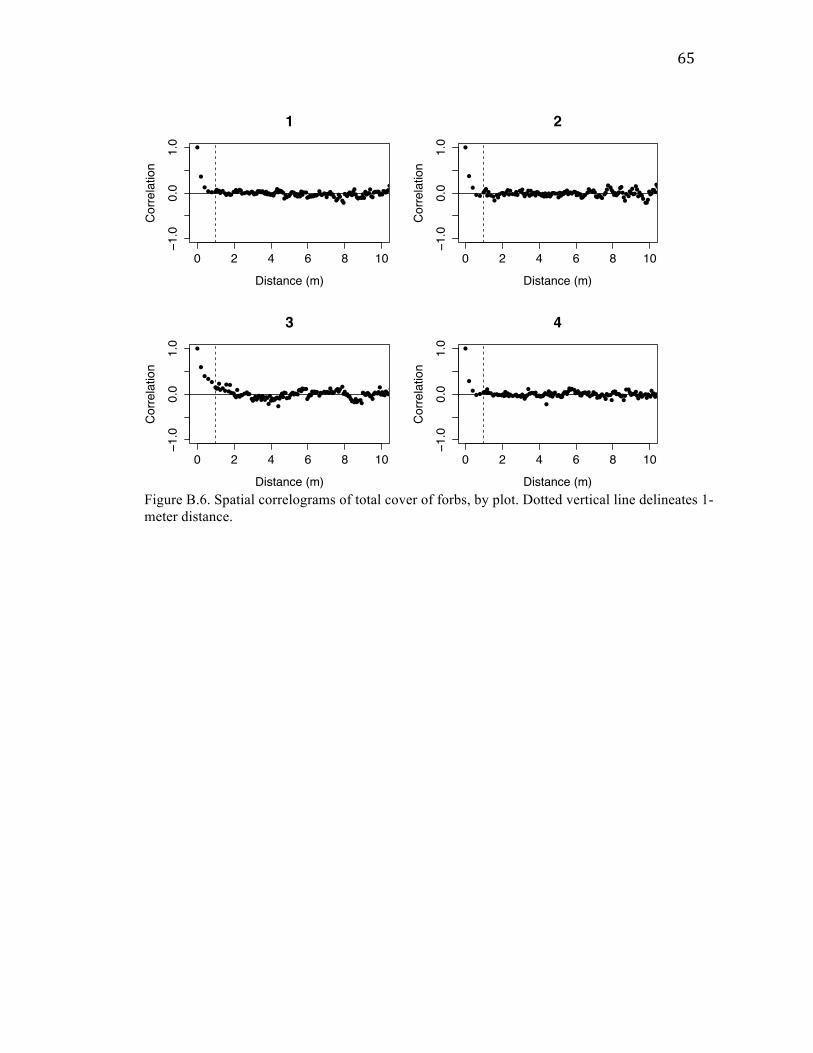
65

Figure B.6. Spatial correlograms of total cover of forbs, by plot. Dotted vertical line delineates 1-meter distance.

●

●

●●●●●●●●●●●●●●

●●●●●●●●●●●●●●●●●●●●●●●●●●●●●●●●

●●●●●●●

●●●●●●●●●●●●●

●●●●●●●●●●●●●

●●●●●●

●●●●●●●●●●●●

●●●●●●●●●●●●●●

●●●●●●●

●●●●●●●●●

●●●●●●●●●●●●

●●●●●●●●●

●●●●●●●●●●●●●

●●●●●●

●●●●●●●●●

●●●●●●

●●●●●●

●●●●●●●●●●

●●

●●●●

●

●

●●●●●●

●●●●

●●●

●

●●●●

●●

●●●●

●

●●●●●●●

●●● ●●●●●●●●●

0 2 4 6 8 10

−1.0

0.0

1.0

1

Distance (m)

Cor

rela

tion

●

●

●

●●●●●●●●●●●●●●●●●

●●●●●●●●

●●●●●●●●●●●●●●●●●●●●●

●●●●●●●●●●

●●●●●●●●●●●●●●●●●●●●●●

●●●●●●

●●●●●●●●●●●●●

●●●●●●●●●●●●●●●●●

●●●●●●●●●●

●●●●●●

●●

●●●●●●●

●●●●●●●●●●

●●●

0 2 4 6 8 10

−1.0

0.0

1.0

2

Distance (m)

Cor

rela

tion

●

●

●●●●●●●●●●

●●●

●●●●

●●●●●

●●●●●●●●●●●●●●●●●●

●

●●●●●●

●

●

●●●●●●●●●●●●●●●

●●●●●●

●●●●●●●●●●

●●●●●●●●●●●●●●●

●

●●●●●●●●●●●●●●●

●●●●●●●●●●●●●

●

●●●●●●●●●●●●●●●

●●●●●●●●●●●●

●●

●

●●●●●●●●●

●

●●

●●

●●●●●●●●

●●●●●

●●●●●●●●●●

●●●●

●●●●●●●

●●●

●●●

●●

●●●

●●●●●●

●●●●●●

●●●●●

●●

●

●

●●

●●

●●

●●

●

●

●

●

●

●●

0 2 4 6 8 10

−1.0

0.0

1.0

3

Distance (m)

Cor

rela

tion

●

●

●●●●

●●●●●●●●●●●●●

●●●●●●●●●●●●●●●

●●●●●●●●●●●●●●●

●

●

●●●●●●●●●●●●

●●●●●●●●●

●●●●●●●●●●●●●

●●●●●●●●●●●●●●

●●●●●●●●●●●●●●●●●●

●●●●●●●●●

●●●●●●●●●

●●●●●●

●

●●●●●●●●

●

●●●●

0 2 4 6 8 10−1

.00.

01.

0

4

Distance (m)

Cor

rela

tion

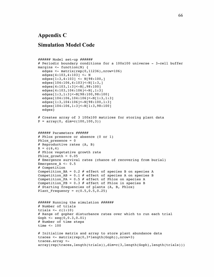
66

Appendix C

Simulation Model Code

###### Model set-up ###### # Periodic boundary conditions for a 100x100 universe - 3-cell buffer margins <- function(N) { edges <- matrix(rep(0,11236),nrow=106) edges[4:103,4:103] <- N edges[1:3,4:103] <- N[98:100,] edges[104:106,4:103]<-N[1:3,] edges[4:103,1:3]<-N[,98:100] edges[4:103,104:106]<-N[,1:3] edges[1:3,1:3]<-N[98:100,98:100] edges[104:106,104:106]<-N[1:3,1:3] edges[1:3,104:106]<-N[98:100,1:3] edges[104:106,1:3]<-N[1:3,98:100] edges} # Creates array of 3 100x100 matrices for storing plant data P = array(0, dim=c(100,100,3)) ###### Parameters ###### # Phlox presence or absence (0 or 1) Phlox_presence = 0 # Reproductive rates (A, B) R = c(6,4) # Phlox vegetative growth rate Phlox_growth = 0.05 # Emergence survival rates (chance of recovering from burial) Emergence_A <- 0.5 # Competition Competition_BA = 0.2 # effect of species B on species A Competition_AB = 0.1 # effect of species A on species B Competition_PA = 0.5 # effect of Phlox on species A Competition_PB = 0.3 # effect of Phlox in species B # Starting frequencies of plants (A, B, Phlox) Plant_Frequency = c(0.5,0.5,0.25) ###### Running the simulation ###### # Number of trials trials <- c(1:10) # Range of gopher disturbance rates over which to run each trial Goph <- seq(0,0.3,0.01) # Number of time steps time <- 100 # Initialize matrix and array to store plant abundance data traces <- matrix(rep(0,3*length(Goph)),nrow=3) traces.array <- array(rep(traces,length(trials)),dim=c(3,length(Goph),length(trials)))

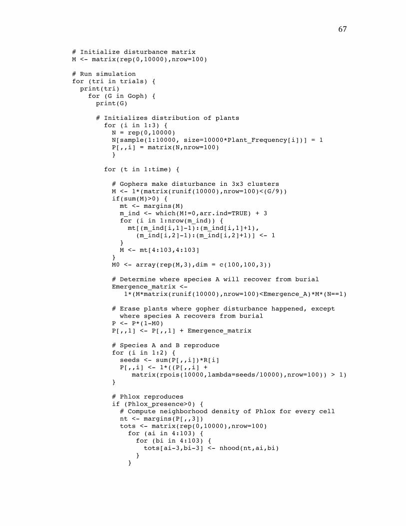
67

# Initialize disturbance matrix M <- matrix(rep(0,10000),nrow=100) # Run simulation for (tri in trials) { print(tri) for (G in Goph) { print(G) # Initializes distribution of plants for (i in 1:3) { N = rep(0,10000) N[sample(1:10000, size=10000*Plant_Frequency[i])] = 1 P[,,i] = matrix(N,nrow=100) } for (t in 1:time) { # Gophers make disturbance in 3x3 clusters M <- 1*(matrix(runif(10000),nrow=100)<(G/9)) if(sum(M)>0) { mt <- margins(M) m_ind <- which(M!=0,arr.ind=TRUE) + 3 for (i in 1:nrow(m_ind)) { mt[(m_ind[i,1]-1):(m_ind[i,1]+1), (m_ind[i,2]-1):(m_ind[i,2]+1)] <- 1 } M <- mt[4:103,4:103] } M0 <- array(rep(M,3),dim = c(100,100,3)) # Determine where species A will recover from burial Emergence_matrix <- 1*(M*matrix(runif(10000),nrow=100)<Emergence_A)*M*(N==1) # Erase plants where gopher disturbance happened, except where species A recovers from burial P <- P*(1-M0) P[,,1] <- P[,,1] + Emergence_matrix # Species A and B reproduce for (i in 1:2) { seeds <- sum(P[,,i])*R[i] P[,,i] <- 1*((P[,,i] + matrix(rpois(10000,lambda=seeds/10000),nrow=100)) > 1) } # Phlox reproduces if (Phlox_presence>0) { # Compute neighborhood density of Phlox for every cell nt <- margins(P[,,3]) tots <- matrix(rep(0,10000),nrow=100) for (ai in 4:103) { for (bi in 4:103) { tots[ai-3,bi-3] <- nhood(nt,ai,bi) } }

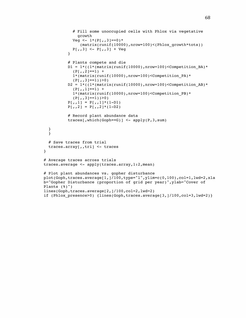
68

# Fill some unoccupied cells with Phlox via vegetative growth Veg <- 1*(P[,,3]==0)* (matrix(runif(10000),nrow=100)<(Phlox_growth*tots)) P[,,3] <- P[,,3] + Veg } # Plants compete and die D1 = 1*((1*(matrix(runif(10000),nrow=100)<Competition_BA)* (P[,,2]==1) + 1*(matrix(runif(10000),nrow=100)<Competition_PA)* (P[,,3]==1))>0) D2 = 1*((1*(matrix(runif(10000),nrow=100)<Competition_AB)* (P[,,1]==1) + 1*(matrix(runif(10000),nrow=100)<Competition_PB)* (P[,,3]==1))>0) P[,,1] = P[,,1]*(1-D1) P[,,2] = P[,,2]*(1-D2) # Record plant abundance data traces[,which(Goph==G)] <- apply(P,3,sum) } } # Save traces from trial traces.array[,,tri] <- traces } # Average traces across trials traces.average <- apply(traces.array,1:2,mean) # Plot plant abundances vs. gopher disturbance plot(Goph,traces.average[1,]/100,type="l",ylim=c(0,100),col=1,lwd=2,xlab="Gopher Disturbance (proportion of grid per year)",ylab="Cover of Plants (%)") lines(Goph,traces.average[2,]/100,col=2,lwd=2) if (Phlox_presence>0) {lines(Goph,traces.average[3,]/100,col=3,lwd=2)}

69

Bibliography

Alatalo, R. V. (1981). Problems in the measurement of evenness in ecology. Oikos, 37(2), 199-204.

Antos, J. A., & Halpern, C. B. (1997). Root system differences among species: implications for early successional changes in forest of Western Oregon. American Midland Naturalist, 138(1), 97-108.

Auerbach, M., & Shmida, A. (1987). Spatial scale and the determinants of plant species richness. Trends in Ecology & Evolution, 2(8), 238-242.

Bates, D. (2006). [R] lmer, p-values and all that. The R-help Archives. https://stat.ethz.ch/pipermail/r-help/2006-May/094765.html

Bates, D., Maechler, M., & Bolker, B. (2011). lme4: Linear mixed-effects models using S4 classes. R package version 0.999375-42. http://CRAN.R-project.org/package=lme4

Bray, J. R., & Curtis, J. T. (1957). An ordination of the upland forest communities of southern Wisconsin. Ecological Monographs, 27(4), 325-349.

Case, M. (2011). Gopher mound disturbance and its consequences for plant communities: past and future research. Junior Paper, Department of Ecology and Evolutionary Biology, Princeton University.

Chaneton, A. E. J., & Facelli, J. M. (1991). Disturbance effects on plant community diversity: spatial scales and dominance hierarchies. Vegetatio, 93(2), 143-155.

Connell, J. H. (1978). Diversity in tropical rain forests and coral reefs. Science, 199(4335), 1302-1310.

Connell, J. H., & Slatyer, R. O. (1977). Mechanisms of succession in natural communities and their role in community stability and organization. The American Naturalist, 111(982), 1119-1144.

D’Antonio, C., & Meyerson, L. A. (2002). Exotic plant species as problems and solutions in ecological restoration: a synthesis. Restoration Ecology, 10(4), 703-713.

Eviner, V. T., & Chapin III, F. S. (2003). Gopher-plant-fungal interactions affect establishment of an invasive grass. Ecology, 84(1), 120–128.

70

Foster, M. A., & Stubbendieck, J. (1980). Effects of the plains pocket gopher (Geomys bursarius) on rangeland. Journal of Range Management, 33, 74-78.

Goslee, S.C. and Urban, D.L. 2007. The ecodist package for dissimilarity-based analysis of ecological data. Journal of Statistical Software, 22(7), 1-19.

Grime, J. R, (1973). Competitive exclusion in herbaceous vegetation. Nature, 242, 344-347.

Grime, J. P. (1979). Plant strategies and vegetation processes. Wiley, Chichester, UK.

Halpern, C. B., Smith, B. G., and Franklin, J. F. (1984). Composition, structure, and distribution of the ecosystems of the Three Sisters Biosphere Reserve/Wilderness Area. A Final Report to the United States Department of Agriculture. 139 p.

Halpern, C. B., Haugo, R. D., Antos, J. A., Kaas, S. S., & Kilanowski, A. L. (2012). Grassland restoration with and without fire: evidence from a tree-removal experiment. Ecological Applications, 22(2), 425-441.

Hastings, A., Byers, J. E., Crooks, J. A., Cuddington, K., Jones, C. G., Lambrinos, J. G., & Talley, T. S. (2007). Ecosystem engineering in space and time. Ecology Letters, 10(2), 153-164.

Hill, M. O. (1973). Diversity and evenness: a unifying notation and its consequences. Ecology, 54(2), 427-432.

Hitchcock, C. L., & Cronquist, A. (1973). Flora of the Pacific Northwest. University of Washington Press, Seattle, Washington.

Hobbs, R. J., & Hobbs, V. J. (1987). Gophers and grassland: a model of vegetation response to patchy soil disturbance. Vegetatio, 69(1), 141-146.

Hobbs, R. J., & Mooney, H. a. (1985). Community and population dynamics of serpentine grassland annuals in relation to gopher disturbance. Oecologia, 67(3), 342-351.

Horn. H. S. (1975). Markovian properties of forest succession. In: Cody. M. L. and Diamond, J. M. (eds), Ecology and evolution of communities. Belknap Press, Cambridge, Massachusetts. 196-211.

Huntly, N., & Reichman, O. J. (1994). Effects of subterranean mammalian herbivores on vegetation. Journal of Mammalogy, 75(4), 852–859.

Inouye, R., Huntly, N., Tilman, D., & Tester, J. (1987). Pocket gophers (Geomys bursarius), vegetation, and soil nitrogen along a successional sere in east central Minnesota. Oecologia, 72, 178–184.

71

Jones, C. C., Halpern, C. B., & Niederer, J. (2008). Plant succession on gopher mounds in Western Cascade meadows: consequences for species diversity and heterogeneity. The American Midland Naturalist, 159(2), 275-286.

Klaas, B. A., Moloney, K. A., & Danielson, B. J. (2000). The tempo and mode of gopher mound production in a tallgrass prairie remnant. Ecography, 23, 246-256.

Knight, J. (2009). Infilled pocket gopher tunnels: seasonal features of high alpine plateaux. Earth Surface Processes and Landforms, 34, 590-595.

Kyle, G. P., Kulmatiski, A., & Beard, K. H. (2008). Influence of pocket gopher mounds on nonnative plant establishment in a shrubsteppe ecosystem. Western North American Naturalist, 68(3), 374–381.

Lammers, D. & Dyrness, T. (2004). Bunchgrass Ridge soil descriptions. http://depts.washington.edu/bgridge/J.PDFs/Bunchgrass_Ridge_pedons.pdf

Lang, N. L., & Halpern, C. B. (2007). The soil seed bank of a montane meadow: consequences of conifer encroachment and implications for restoration. Canadian Journal of Botany, 85(6), 557-569.

Levin, S. A. (1992). The problem of pattern and scale in ecology: The Robert H. MacArthur Award Lecture. Ecology, 73(6), 1943.

Lezberg, A. L., Antos, J. A., & Halpern, C. B. (1999). Belowground traits of herbaceous species in young coniferous forests of the Olympic Peninsula, Washington. Canadian Journal of Botany, 77, 936-943.

Mackey, R. L., & Currie, D. J. (2001). The diversity-disturbance relationship: is it generally strong and peaked? Ecology, 82(12), 3479-3492.

MacArthur, R. H., and E. O. Wilson. (1967). The theory of island biogeography. Princeton University Press, Princeton, New Jersey.

Magurran, A. E. (2004). Measuring biological diversity. Blackwell Publishing, Malden, Massachusetts.

Martinsen, G. D., Cushman, J. H., & Whitham, T. G. (1990). Impact of pocket gopher disturbance on plant species diversity in a shortgrass prairie community. Oecologia, 83(1), 132-138.

McCain, K. N. S., Baer, S. G., Blair, J. M., & Wilson, G. W. T. (2010). Dominant grasses suppress local diversity in restored tallgrass prairie. Restoration Ecology, 18(September), 40-49.

72

Mielke, H. W. (1977). Mound building by pocket gophers (Geomyidae): their impact on soils and vegetation in North America. Journal of Biogeography, 4(2), 171.

Moloney, K. A., & Levin, S. A. (1996). The effects of disturbance architecture on landscape-level population dynamics. Ecology, 77(2), 375–394.

Oksanen, J., Blanchet, F. G., Kindt, R., Legendre, P., Minchin, P. R., O'Hara, R. B., Simpson, G. L., Solymos, P., Stevens, M. H. H. & Wagner, H. (2011). vegan: Community Ecology Package. R package version 2.0-2. http://CRAN.R-project.org/package=vegan

Overton, J., & Levin, S. A. (2003). Components of spatial patterning in a serpentine grassland. Ecological Research, 18(4), 405-421.

Platt W. J. (1975). The colonization and formation of equilibrium plant species associations on badger disturbance in a tall-grass prairie. Ecological Monographs, 45, 285-305.

R Development Core Team (2011). R: A language and environment for statistical computing. R Foundation for Statistical Computing, Vienna, Austria. ISBN 3-900051-07-0, URL http://www.R-project.org/.

Reice, S. R. (1994). Nonequilibrium determinants of biological community structure. American Scientist, 82(5), 424-435.

Reichman, O. J. (2007). The influence of pocket gophers on the biotic and abiotic environment. Subterranean Rodents (pp. 271–286). Springer. Retrieved from http://www.springerlink.com/index/g64726713h601695.pdf

Reichman, O. J., & Seabloom, E. W. (2002). The role of pocket gophers as subterranean ecosystem engineers. Trends in Ecology & Evolution, 17(1), 44-49.

Rogers, W. E., & Hartnett, D. C. (2001). Temporal vegetation dynamics and recolonization mechanisms on different-sized soil disturbances in tallgrass prairie. American Journal of Botany, 88(9), 1634-1642.

Rogers, W., Hartnett, D., & Elder, B. (2001). Effects of plains pocket gopher (Geomys bursarius) disturbances on tallgrass-prairie plant community structure. The American Midland Naturalist, 145(2), 344-357.

Schaal, B. A., Leverich, W. J. (1982). Survivorship patterns in an annual plant community. Oecologia, 54, 149–151.

Seabloom, E. W., & Reichman, O. J. (2001). Simulation models of the interactions between herbivore foraging strategies, social behavior, and plant community dynamics. The American Naturalist, 157(1), 76-96.

73

Sherrod, S. K., & Seastedt, T. R. (2001). Effects of the northern pocket gopher (Thomomys talpoides) on alpine soil characteristics, Niwot Ridge, CO. Biogeochemistry, 55(2), 195–218.

Sherrod, S. K., Seastedt, T. R., & Walker, M. D. (2005). Northern pocket gopher (Thomomys talpoides) control of alpine plant community structure. Arctic, Antarctic, and Alpine Research, 37(4), 585–590.

Smallwood, K. S., & Morrison, M. L. (1999). Estimating burrow volume and excavation rate of pocket gophers (Geomyidae). The Southwestern Naturalist, 44(2), 173–183.

Sousa, W. P. (1984). The role of disturbance in natural communities. Annual Review of Ecology and Systematics, 15, 353-391.

Thomson, J. D., Weiblen, G., Thomson, B. A., Alfaro, S., & Legendre, P. (1996). Untangling multiple factors in spatial distributions: lilies, gophers, and rocks. Ecology, 77(6), 1698-1715.

Tilman, D. (1983). Plant succession and gopher disturbance along an experimental gradient. Oecologia, (60), 285-292.

Tremblay, A. (2011). LMERConvenienceFunctions: A suite of functions to back-fit fixed effects and forward-fit random effects, as well as other miscellaneous functions. R package version 1.6.7. http://CRAN.R-project.org/package=LMERConvenienceFunction

Venables, W. N. & Ripley, B. D. (2002) Modern Applied Statistics with S. Fourth Edition. Springer, New York.

Watts, S. M. (2010). Pocket gophers and the invasion and restoration of native bunchgrass communities. Restoration Ecology, 18(1), 34-40.

Western Regional Climate Center. Santiam Pass, Oregon: period of record monthly climate summary. http://www.wrcc.dri.edu/cgi-bin/cliMAIN.pl?orsant. Accessed February 2012.

Wolfe-Bellin, K. S., & Moloney, K. A. (2000). The effect of gopher mounds and fire on the spatial distribution and demography of a short-lived legume in tallgrass prairie. Canadian Journal of Botany, 78(10), 1299-1308.

Wu, J., & Levin, S. A. (1994). A spatial patch dynamic modeling approach to pattern and process in an annual grassland. Ecological Monographs, 64(4), 447–464.

Zuur, A. F., Ieno, E. N., Walker, N. J., Saveliev, A. A., & Smith, G. M. (2009). Mixed effects models and extensions in ecology with R. Springer, New York.

74

This paper represents my own work in accordance with University regulations.

_______________________________