Goal

• A tutorial overview of wireless communication– Antennas, propagation and (de)modulation

• Focus on a single wireless link– Operating on a small slice of spectrum called a

“channel”, characterized by centre frequency and bandwidth

1

• application: supporting network applications– FTP, SMTP, HTTP

• transport: process-process data transfer– TCP, UDP

• network: routing of datagrams from source to destination– IP, routing protocols

• link: data transfer between neighboring network elements– PPP, Ethernet

• physical: bit pipe

Internet Protocol Stack

application

transport

network

link

physical

source

applicationtransportnetwork

linkphysical

HtHn M

segment Htdatagram

destination

applicationtransportnetwork

linkphysical

HtHnHl M

HtHn M

Ht M

M

networklink

physical

linkphysical

HtHnHl M

HtHn M

HtHnHl M

router

switch

message M

Ht M

Hnframe

HtHnHl M

Digital Communication System

4

Source Encoder

Channel

Channel Encoder Channel Decoder

Source Decoder

Source Destination

Bit stream for

transmissionReceived

bit stream

Transmitted

waveform

Received

waveform

Physical Layer

Channel Encoder/Decoder Layers

1. Error Correction Coder/Decoder2. Modulator/Demodulator (Baseband)3. Frequency Conversion (Passband)

5

Wireless Communication System

6

Source Encoder

Channel Encoder Channel Decoder

Source Decoder

Source Destination

Bit stream for

transmissionReceived

bit stream

Transmitted

waveform

Received

waveform

Physical Layer

Wireless channel

Antenna Antenna

Antennas

8

Antenna

• Antenna design goal: ensure the conversion process is efficient, i.e., direct as much power as possible in “useful” directions

9

Field Regions

• L (antenna diameter) and λ (wavelength)

10

Antenna Radiation Pattern

• Plot of far-field radiation from the antenna– Radiation intensity, U: power radiated from an antenna per unit

solid angle– Isotropic antenna with spherical pattern vs. omnidirectional (e.g.,

hertzian dipole) vs. directional

• Azimuth plane (x-y plane), Elevation plane (x-z plane)

11

Antenna Radiation Pattern (contd.)

Hertzian Dipole Antennay

x

z

Isotropic Antenna

12

Radiation Pattern of a Generic Directional Antenna

• Half-power beamwidth (HPBW): angle subtended by the half-power points of the main lobe

• Front-back ratio: ratio between peak amplitudes of main and back lobes

• Side lobe level: amplitude of the biggest side lobe

13

Antenna Directivity, Efficiency and Gain

• Directivity, D: ratio of max radiation intensity of antenna to radiation intensity of isotropic antenna radiating the same total power– D ~ 41,000/Θo

HPφoHP ; Θo

HP ( φoHP ) are vertical (horizontal) plane

half-power beamwidths in degrees

• Radiation Efficiency, e: ratio of radiated power to power accepted by antenna– Sometimes specified via Voltage Standing Wave Ratio (VSWR)

• (Power) Gain, G = e * D

14

Antenna Polarization

• Orientation of the electric field of an electromagnetic wave relative to the earth

• In general described by an ellipse

• Two special cases of elliptical polarization: linear and circular polarizations

15

Electromagnetic Wave Propagation

Wireless Propagation

16

17

Decibels• Power ratio in decibels = 10log10(P/Pref)

– Power ratios 101 10dB, 102 20dB, 103 30dB, …– Similarly, power ratios 10-1 -10dB, 10-2 -20dB, 10-3 -30dB, …– 3dB (power ratio = 2), -3dB (power ratio = ½)

• Voltage ratio in decibels = 20log10(V/Vref), since P = V2/R• Absolute power with respect to standard reference power in decibels:

dBW (Pref = 1W) and dBm (Pref = 1mW)– 1W = 0 dBW = +30 dBm; 1mW = 0 dBm = -30 dBW

• Antenna gains: dBi (Pref is power radiated by an isotropic reference antenna) and dBd (Pref is power radiated by a half-wave dipole)– 0 dBd = 2.15 dBi

• dB for gains and losses (e.g., path loss, SNR)• Why in decibels?

– Signal strength often falls off exponentially, so loss easily expressed in terms of decibel (a logarithmic unit)

– Net gain or loss via simple addition and subtraction

18

Noise Types in a Wireless Channel

• Multiplicative– Antenna directionality– Attenuation or Absorption (walls,

trees, atmosphere)– Reflection (smooth surfaces)– Scattering (rough surfaces and

small objects)– Refraction (atmospheric layers,

layered/graded materials)– Diffraction (edges of buildings

and hills)

• Additive– Internal sources within the

receiver: thermal and shot noise in passive and active components

– External sources: Interference from other

transmitters and appliances Atmospheric effects Cosmic radiation

19

Three Scales of Multiplicative Noise

• Large-scale propagation effects– Path loss– Shadowing (or slow fading)

leads to variations over distances in the order of metres Could be over 10s or 100s of

metres in outdoor environments

• Fast fading (or multipath fading), a small-scale propagation effect: causes variations of over very short distances in the order of the signal wavelength

20

Fading Processes Illustrated

21

Another Illustration of Path Loss, Shadowing and Multipath Fading

22

Path Loss

• Received power, PR = PTGTGR/LTLLR

• Effective Isotropic Radiated Power (EIRP)– At transmitter, PTI = PTGT/LT

– At receiver, PR = PRIGR/LR

• Path loss, L = PTI/PRI = PTGTGR/PRLTLR

Free-Space (or Spreading) Loss Illustration on a Point-to-Point Wireless Link

• Assume antennas T and R– Arranged such that

their directions of maximum gain are aligned

– With matching polarizations

– Separated by distance d, large enough that antennas are in each other’s far-field regions

23

24

Free-Space Loss• For simplicity, assume no feeder losses, i.e., LT = LR = 1• PT: transmit power• S: power density incident on receiver antenna =

PTGT/4Πd2

• Receiver antenna effective area (aperture), AeR = GR λ2 /4Π • Receiver input power, PR = PTGTAeR/4Πd2

• Friss transmission formula: PR/PT = GTGR(λ/4Πd)2

• Propagation loss in free space, LF = PTGTGR/PR = (4Πd/λ)2

= (4Πdf/c)2

– c, speed of light (3 x 105 Km per second)• LF (dB) = 32.4 + 20log(d) + 20log(f), d in Km and f in MHz

Path Loss Exponent (α)

• Free-space loss is the minimum path loss for a given distance

• Path loss in practice much higher (includes average shadowing) because of attenuation due to signal encounters with the environment

• Path loss exponent, α: a term used to indicate how fast signal power degrades with distance– α = 2 in free space; typically, 2 ≤ α ≤ 5

25

26

Two-Ray (Plane Earth Loss) Model

• PR = PTGTGR(hthr)2/r4

27

Two-Slope Model [Schwartz’05]• Two-ray model only holds for

long distances– Oscillation at short distances

due to the constructive and destructive combination of the two rays

• Instead, two-slope model used (for microcells)

City n1 n2 db(m)

London 1.7-2.1 2-7 200-300

Melbourne 1.5-2.5 3-5 150

Orlando 1.3 3.5 90

Receiver Sensitivity

• Received power level, PRmin, at which just

acceptable communication quality– Assuming only thermal noise in the receiver electronic

circuitry– For a given transmission bit-rate (i.e., physical layer

data rate)– Determines maximum range

• Path loss corresponding to PRmin is called

maximum acceptable path loss

28

29

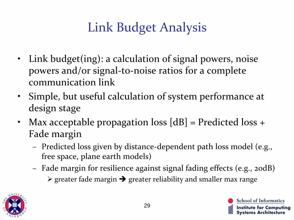
Link Budget Analysis

• Link budget(ing): a calculation of signal powers, noise powers and/or signal-to-noise ratios for a complete communication link

• Simple, but useful calculation of system performance at design stage

• Max acceptable propagation loss [dB] = Predicted loss + Fade margin– Predicted loss given by distance-dependent path loss model (e.g.,

free space, plane earth models)– Fade margin for resilience against signal fading effects (e.g., 20dB)

greater fade margin greater reliability and smaller max range

30

Shadowing• Represents medium-scale fluctuations of the

received signal power occurring over distances from few metres to tens or hundreds of meters

• Due to signal encounters with terrain obstructions such as hills or man-made obstructions (e.g., buildings, trees)

• Measured signal power may differ substantially at different locations even though at the same radial distance from transmitter

31

Multipath Fading• Effects

– Rapid changes in signal strength over a small physical distance or time interval

– Time dispersion (echoes) caused by multipath propagation delays

– Random frequency modulation due to Doppler shifts on different multipath signals

• Influencing Factors– Multipath propagation– The transmission

bandwidth of the signal

– Speed of the mobile– Speed of surrounding

objects

32

Multipath Propagation(a) constructive phase interference (b) destructive phase

interference

Delay Spread• Depends on the environment

– Typically around 40-70ns in indoor office environments, can go up to 200ns in some cases

• Can cause inter-symbol interference (ISI)

33

34

Doppler Shift• Vehicle motion with respect to the incoming ray

introduces a doppler frequency shift, fk = vcosβk/λ Hz

• Frequency of received signal with doppler shift = fc + fk, where fc is carrier frequency

35

Multipath Channel Parameters• Doppler spread (BD) and coherence time (TC) describe the

time-varying (frequency dispersive) nature of the channel due to relative motion of transmitter and receiver or movement of surrounding objectsTC α 1/BD

• Delay spread (τt) and coherence bandwidth (Bc) describe the frequency-selective (time dispersive) nature of the channel due to delays between different propagation pathsΤt α 1/Bc

36

Mitigating Multipath Fading

• Coding techniques for error detection and correction

• Interleaving for combating fast fading• Diversity techniques (space, frequency, time and

polarization dimensions)• Equalization also to mitigate frequency-selective

fading• Orthogonal frequency division multiplexing

(OFDM) to mitigate frequency-selective fading

Signal-to-Noise Ratio (SNR)• Crucial factor determining

wireless transmission quality

• Shannon’s Channel Capacity Theorem for band-limited additive white Gaussian noise (AWGN) channel: C = W log2(1+SNR)– C, channel capacity in bits

per second– W, channel bandwidth in

Hz– SNR, signal-to-noise ratio

• So long as data rate below C, error probability can made arbitrarily lower with the use of more sphisticated coding schemes

37

SNR versus Distance

38

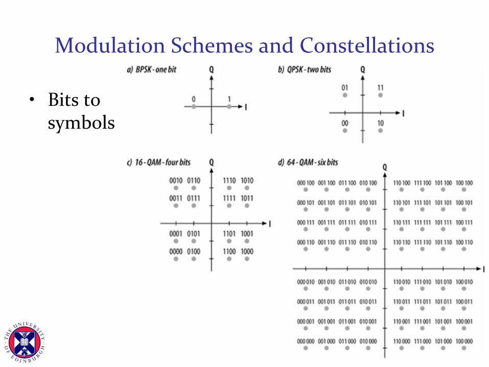
Modulation Schemes and Constellations

• Bits to symbols

39

Wireless Link Throughput

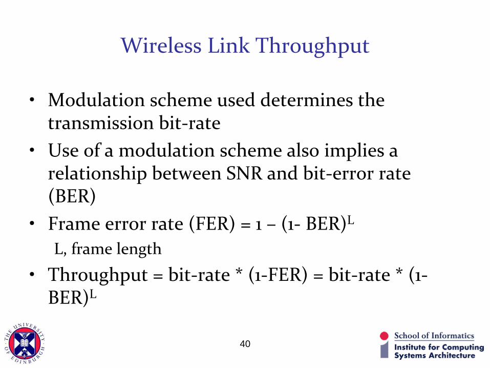
• Modulation scheme used determines the transmission bit-rate

• Use of a modulation scheme also implies a relationship between SNR and bit-error rate (BER)

• Frame error rate (FER) = 1 – (1- BER)L

L, frame length

• Throughput = bit-rate * (1-FER) = bit-rate * (1-BER)L

40

BER versus SNR

• Assume a symbol rate of 1M symbols per second and AWGN channel

41

Bit-Level Throughput versus SNR

42

Frame-Level Throughput versus SNR

43

Error Correction Coding and Coding Rate (R)

• Determines the number of redundant bits added

• Ratio of number of data bits transmitted to the number of coded bits

• If K redundant bits are added for every N data bits transmitted, then R = N / (N+K)

44

Orthogonal Frequency Division Multiplexing (OFDM)• A wide channel is divided into several component

“orthogonal” subcarriers• Use multiple subcarriers in parallel for a single

transmission by multiplexing data over all of them• Physical layer in 802.11a/g is based on OFDM• Similar to the discrete multi-tone (DMT) in DSL systems

45

The 802.11a/g Case

• Total 52 subcarriers for a 20MHz channel– 48 subcarriers used for data and the remaining 4 are

pilot subcarriers

46

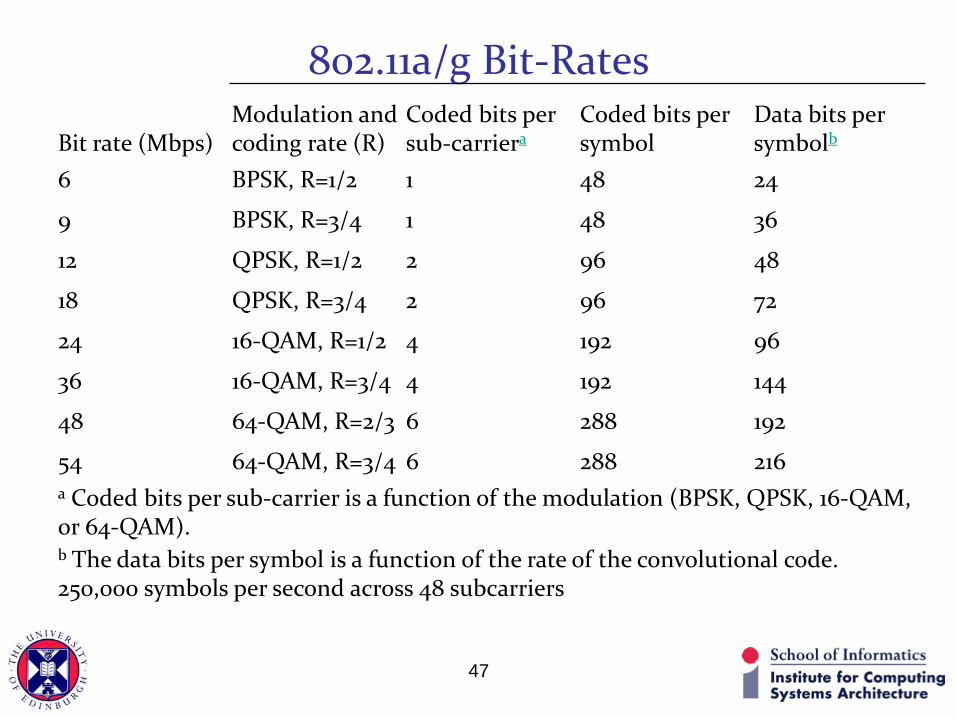
802.11a/g Bit-Rates

Bit rate (Mbps)Modulation and coding rate (R)

Coded bits per sub-carriera

Coded bits per symbol

Data bits per symbolb

6 BPSK, R=1/2 1 48 24

9 BPSK, R=3/4 1 48 36

12 QPSK, R=1/2 2 96 48

18 QPSK, R=3/4 2 96 72

24 16-QAM, R=1/2 4 192 96

36 16-QAM, R=3/4 4 192 144

48 64-QAM, R=2/3 6 288 192

54 64-QAM, R=3/4 6 288 216a Coded bits per sub-carrier is a function of the modulation (BPSK, QPSK, 16-QAM, or 64-QAM).b The data bits per symbol is a function of the rate of the convolutional code.250,000 symbols per second across 48 subcarriers

47

Multiple Access Techniques

• Frequency Division Multiple Access (FDMA)

• Time Division Multiple Access (TDMA)

• Code Division Multiple Access (CDMA)

48

Frequency Division Multiple Access (FDMA)

• Early cellular systems were based on (analog) FDMA

• OFDM (and OFDMA) similar to FDMA, except frequency division done digitally– Closer frequency spacing– Dynamic allocation of subcarriers (in WiMAX and

LTE)

49

frequency

time

Time Division Multiple Access (TDMA)

• More difficult to implement than FDMA since the users must be time-synchronized

• But easier to accommodate multiple data rates with TDMA since multiple timeslots can be assigned to a given user

• Random access: “asynchronous” version of TDMA – ALOHA, Slotted ALOHA, CSMA, CSMA/CD

(Ethernet), CSMA/CA (WiFi)50

frequency

time

Wireless Random Multiple Access Issues• Half-duplex operation collision detection at

transmitter very difficult• Location-dependent carrier sensing

– Hidden terminals– Exposed terminals– Capture

51

Code Division Multiple Access (CDMA)

• Used in several wireless broadcast channel standards (e.g., 2G/3G cellular, satellite)

• Unique “code” assigned to each user; i.e., code set partitioning

• All users share same frequency, but each user has own “chipping” sequence (i.e., code) to encode data

• Encoded signal = (original data) X (chipping sequence)• Decoding: inner-product of encoded signal and

chipping sequence• Allows multiple users to “coexist” and transmit

simultaneously with minimal interference (if codes are “orthogonal”)

• Issues: code selection, near-far problem

53

(a) FDMA, (b) TDMA, (c) CDMA.

CDMA Encode/Decode

slot 1 slot 0

d1 = -1

1 1 1 1

1- 1- 1- 1-

Zi,m= di.cm

d0 = 1

1 1 1 1

1- 1- 1- 1-

1 1 1 1

1- 1- 1- 1-

1 1 11

1-1- 1- 1-

slot 0channeloutput

slot 1channeloutput

channel output Zi,m

sender

code

databits

slot 1 slot 0

d1 = -1

d0 = 1

1 1 1 1

1- 1- 1- 1-

1 1 1 1

1- 1- 1- 1-

1 1 1 1

1- 1- 1- 1-

1 1 11

1-1- 1- 1-

slot 0channeloutput

slot 1channeloutput

receiver

code

receivedinput

Di = Σ Zi,m.cm

m=1

M

M

6: Wireless and Mobile Networks6-55

CDMA: two-sender interference

References• R. G. Gallager, Principles of Digital

Communication, Cambridge University Press, 2008.

• S. R. Saunders and A. Aragon-Zavala, “Antennas and Propagation for Wireless Communication Systems,” Second Edition, John Wiley, 2007.

• M. Schwartz, “Mobile Wireless Communications,” Cambridge University Press, 2005.

• C. Haslett, “Essentials of Radio Wave Propagation,” Cambridge University Press, 2008.

• E. McCune, Practical Digital Wireless Signals, Cambridge University Press, 2010.

56

References (Contd.)

• M. S. Gast, “802.11 Wireless Networks,” O’Reilly, 2005.

• J. C. Bicket, “Bit-Rate Selection in Wireless Networks,” Master’s thesis, MIT, Feb 2005.

• J. F. Kurose and K. W. Ross, “Computer Networking: A Top-Down Approach,” 5th edition, Pearson Education, 2010.

• A. C. V. Gummalla and J. O. Limb, “Wireless Medium Access Control Protocols,” IEEE Communications Surveys & Tutorials, 2000.

• C. Cox, “Essentials of UMTS,” Cambridge University Press, 2008. 57