ABSTRACT

SHENG, XINXIN. Goal-Based Agent Design: Decision Making in General Game

Playing. (Under the direction of Professor David Thuente.)

General Game Playing's primary research thrust is building automated intelligent

computer agents that accept declarative descriptions of arbitrary games at run-time

and are capable of using such descriptions to play effectively without human

intervention. The research in general game playing approximates human cognitive

processes, sophisticated planning, and problem solving with an instant reward system

represented in games. General game playing has well-recognized research areas with

diverse topics including knowledge representation, search, strategic planning, and

machine learning. It attacks the general intelligence problem that Artificial

Intelligence researchers have made little progress on for the last several decades.

We have designed and implemented an automated goal-based general game playing

agent that is capable of playing most games written in the Game Description

Language and has shown excellent results for general-purpose learning in the general

game playing environment. Our contributions include: the general game playing

agent designed to play a wide variety of games, the knowledge reasoning performance

improvement algorithm, the run-time feature identification algorithm, the contextual

decision-making algorithm, and the GDL extension to enrich the game domain.

Goal-Based Agent Design: Decision Making in General Game Playing

by

Xinxin Sheng

A dissertation submitted to the Graduate Faculty of

North Carolina State University

in partial fulfillment of the

requirements for the degree of

Doctor of Philosophy

Computer Science

Raleigh, North Carolina

2011

APPROVED BY:

_______________________________ ______________________________

Professor David Thuente Professor Peter Wurman

Chair of Advisory Committee

_______________________________ ______________________________

Professor James Lester Professor Munindar Singh

_______________________________

Professor Robert Michael Young

ii

DEDICATION

To my husband Qian Wan, for keeping my soul not lonely.

iii

BIOGRAPHY

Xinxin Sheng (盛欣欣) was born in Qingdao, China to Qinfen Guo (郭琴芬) and

Zhengyi Sheng (盛正沂). She attended Shandong University for undergraduate in

English Language and Literature from 1995 to 1999 and received the second

Bachelor's degree from Tsinghua University in Computer Science in 2002. She

moved to Raleigh, USA the following year. After graduated from North Carolina

State University with a Master of Science degree in 2005, she continued into the Ph.D

program in Computer Science. She has published with several Artificial Intelligence

conferences and journals, and served as program committee member and reviewer for

international computer science conferences. In addition to academic endeavors, she

worked for SGI (2001), Schlumberger (2002-2003), IBM (2006-2011), and joins

Armanta Inc. upon graduation.

iv

ACKNOWLEDGMENTS

I am indebted to my advisor, David Thuente, for his incisive advice and his gracious

guidance. He has been so supportive and so encouraging that working with him has

been absolutely productive. I would like to thank Dr. Peter Wurman for introducing

me to artificial intelligence research. He opened a door to so many opportunities and

excitements -- the wonderland that I will continue surfing for many years to come.

I am grateful that Michael Genesereth sponsored the annual AAAI general game

playing competition. Thanks to the GGP workshop in Barcelona, I had enlightening

discussions with Michael Thielscher, Daniel Michulke, Hilmar Finnsson, Nathan

Sturtevant, and Stephan Schiffel, who also maintains the Dresden GGP website.

In the eight years of my Ph.D endeavors, my husband Qian Wan has stood beside me

no matter how difficult the situations were, in sickness and in poor. My parents have

urged me never settle for anything less than that of which I am capable. Michael

Smith, Joel Duquene, and Jane Revak have inspired me and encouraged me to stand

behind my own choices and not to give up because it is hard. They have mentored me

for both professional advances and character development.

I also appreciate that North Carolina State University sponsored my graduate study

for five years. My research would not have been possible without it.

v

TABLE OF CONTENTS

List of Figures.............................................................................................................ix

List of Tables...............................................................................................................xi

1 Introduction .......................................................................................................... 1

1.1 History of General Game Playing Research .................................................... 3

1.2 General Game Playing Framework ................................................................. 4

1.2.1 Multi-Agent Game Playing System ....................................................... 4

1.2.2 Game Description Language ................................................................. 5

1.2.3 Dedicated Games ................................................................................... 6

1.3 Research Status in General Game Playing ...................................................... 7

1.4 Contributions and Limitations of Our GGP Player ....................................... 11

2 Game Description Language .............................................................................. 14

2.1 Syntactic and Semantic Definition ................................................................ 14

2.2 Game Relations Definition ............................................................................ 15

2.3 Multi-Agent System Communication Protocol ............................................. 16

2.4 Reasoning with GDL ..................................................................................... 18

2.5 Development of GDL .................................................................................... 18

3 Designing the GGP Agent .................................................................................. 20

3.1 Heuristic Search ............................................................................................. 22

3.2 Logic Resolution ........................................................................................... 25

3.3 Learning ......................................................................................................... 26

3.4 Game Examples ............................................................................................. 29

4 Knowledge Representation and Reasoning ........................................................ 34

4.1 Reasoning with Logic: Substitution, Unification and Backward Chaining .. 34

4.2 Limitations of the Knowledge Base .............................................................. 36

vi

4.3 Using Hash Tables to Expedite Reasoning ................................................... 38

4.4 Hash Tables Performance Analysis ............................................................... 46

5 Sub-Goal Identification ...................................................................................... 53

5.1 Generating Training Set with Simulation ...................................................... 53

5.1.1 Random Simulation versus Active Learning ....................................... 54

5.1.2 Determining the Simulation Size ......................................................... 56

5.1.3 Out of Scope Situations ....................................................................... 57

5.2 Identify the Sub-Goals ................................................................................... 58

5.3 Sub-Goal Analysis Example .......................................................................... 59

5.3.1 Statistical Analysis .............................................................................. 60

5.3.2 Sub-Goals versus Actual Goals ........................................................... 63

5.3.3 Using Sub-Goals in Game Play ........................................................... 64

5.4 Experiments for Generality ........................................................................... 66

6 Decision Making in GGP ................................................................................... 71

6.1 Grouping of Sub-Goals .................................................................................. 71

6.2 Decision Trees ............................................................................................... 72

6.2.1 Decision Tree C4.5 Algorithm ............................................................ 72

6.2.2 Build C4.5 with Sub-Goals .................................................................. 76

6.2.3 Using Decision Tree for Evaluation .................................................... 78

6.2.4 Decision Tree Learning versus Individual Sub-Goal Learning ........... 81

6.2.5 Time Cost of Using Decision Tree Algorithm .................................... 88

6.2.6 Overfitting Concerns ........................................................................... 90

6.3 Contextual Decision Tree .............................................................................. 91

6.3.1 Decisions Bounded by Search ............................................................. 91

6.3.2 Building Contextual Decision Trees ................................................... 92

6.3.3 Using Contextual Decision Trees for State Evaluation ....................... 96

vii

6.3.3.1 Comparison with Other Learning Algorithms ............................. 96

6.3.3.2 Comparison with Other Widely Available GGP Players ............. 99

6.3.3.3 Comparison with Human Expert Game Strategies .................... 101

6.3.4 Time Cost of Contextual Decision Trees .......................................... 102

7 Beyond the Current GGP Framework .............................................................. 105

7.1 Issues with the Current GDL ....................................................................... 105

7.1.1 Burden of the Natural Numbers ........................................................ 106

7.1.2 Confusion of the Comparison ............................................................ 108

7.1.3 Challenge of Infinity .......................................................................... 110

7.2 Extension Implementation ........................................................................... 111

7.3 Impact of the Extension ............................................................................... 118

7.4 Extension Application to Coalition Games ................................................. 119

7.4.1 Coalition Games ................................................................................ 119

7.4.2 Coalition Farmer Game ..................................................................... 120

7.5 Benefits and Concerns ................................................................................. 125

8 Summary .......................................................................................................... 128

9 Future Work ..................................................................................................... 130

9.1 GGP Definition ............................................................................................ 130

9.2 GGP Competition ........................................................................................ 131

9.3 GGP Evaluation ........................................................................................... 133

References................................................................................................................135

Appendices...............................................................................................................142

Appendix A General Game Playing Example Game List................................143

Appendix B Full Tic-Tac-Toe Game Description in GDL..............................148

Appendix C Full Othello Game Description in GDL......................................151

viii

Appendix D A Complete Tic-Tac-Toe Match with HTTP Communications..161

Appendix E GGP Agent Descriptions and Experiment Set-up........................165

ix

LIST OF FIGURES

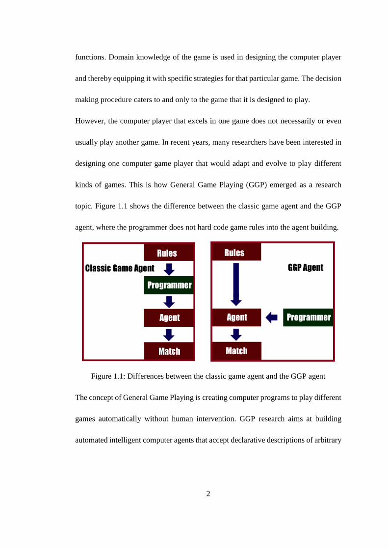
Figure 1.1: Differences between the classic game agent and the GGP agent ............. 2

Figure 3.1: Architecture of our General Game Playing agent ................................... 21

Figure 3.2: Pseudo-code for minimax search in general games ................................ 24

Figure 3.3: General game examples I ........................................................................ 29

Figure 3.4: General game examples II ...................................................................... 31

Figure 4.1: Tic-Tac-Toe example .............................................................................. 35

Figure 4.2: Tic-Tac-Toe hash table mapping example .............................................. 39

Figure 4.3: Pseudo-code for converting GDL sentences into hash tables ................. 43

Figure 4.4: Normalized time cost comparison to find legal actions .......................... 47

Figure 4.5: Normalized time cost comparison to play with random actions ............. 48

Figure 4.6: Normalized time cost comparison to search one-step for goals ............. 49

Figure 5.1: Tic-Tac-Toe X-player winning features based on 95% confidence interval

................................................................................................................................... 61

Figure 5.2: Tic-Tac-Toe middle game example ........................................................ 63

Figure 5.3: Tic-Tac-Toe X-player winning rate against random O-player ............... 66

Figure 5.4: Heated map of the Connect Four board positions ................................... 67

Figure 5.5: Initial state of the Mini-Chess game and its top three sub-goals ............ 68

x

Figure 5.6: Performance comparison of random player, one-step goal-search player,

and sub-goal learning player ..................................................................................... 70

Figure 6.1: Pseudo-code for decision tree C4.5 ........................................................ 73

Figure 6.2: A decision-tree example ......................................................................... 77

Figure 6.3: Pseudo-code of using decision tree for state evaluation ......................... 79

Figure 6.4: Evaluating searched states in a partial game tree .................................... 80

Figure 6.5: Mini-Chess: winning rate for four White players ................................... 83

Figure 6.6: Connect Four: winning rate for four White players ................................ 85

Figure 6.7: Crossing Chinese Checkers: winning rate for four Red (first) players ... 86

Figure 6.8: Ten-iteration Farmer game: winning rate for Alice ................................ 88

Figure 6.9: State changes in game playing ................................................................ 93

Figure 6.10: Pseudo-code for creating contextual decision tree ................................ 95

Figure 6.11: Winning rate comparison of five different playing strategies .............. 98

Figure 6.12: Connect Four: intermediate game examples (Allis, 1988) ................. 101

Figure 7.1: Arithmetic addition defined with GDL in the Farmer game ................. 107

Figure 7.2: Pseudo-code for extending GDL to call external resources .................. 113

Figure 7.3: Normal distribution of the amount of the money the players made in

different scenarios ................................................................................................... 122

xi

LIST OF TABLES

Table 4.1: The average number of knowledge base visits during random matches .. 37

Table 4.2: Agent time usage (milliseconds) .............................................................. 50

Table 4.3: Agent memory usage (bytes) .................................................................... 51

Table 6.1: Execution time comparison: goal-search versus decision tree ................. 89

Table 6.2: Execution time comparison (seconds) .................................................... 103

1

1 Introduction

Games have fascinated humans for centuries. “The term game refers to those

simulations which work wholly or partly on the basis of a player’s decisions.”

(Angelides, 1993). Games are, in fact, abstract models of real-world logics. Computer

game playing research covers many Artificial Intelligence (AI) topics such as

goal-based agent design, massive search, decision making, and machine learning.

Scientists simulate games on computers with software programs and work very hard

to improve the performances of computer game players. Programming an automated

game playing agent that can challenge, even overcome, human experts in

competitions has been a goal for many computer scientists for several decades. Some

game playing programs have proven to be very successful: Chinook (Schaeffer, 1997)

became the world champion Checkers player in 1989 and Deep Blue (Hsu, 2002) the

world Chess champion in 1997. The success of Deep Blue became the milestone

showing that computer game playing exhibited "human comparable" intelligent

behavior, i.e., passed the Turing test (Turing, 1950) in Chess.

In contrast to human players, these successful computer game players usually

capitalize on their computational strength with powerful search techniques that use

enormous game sub-trees and extensive opening and closing books for evaluation

2

functions. Domain knowledge of the game is used in designing the computer player

and thereby equipping it with specific strategies for that particular game. The decision

making procedure caters to and only to the game that it is designed to play.

However, the computer player that excels in one game does not necessarily or even

usually play another game. In recent years, many researchers have been interested in

designing one computer game player that would adapt and evolve to play different

kinds of games. This is how General Game Playing (GGP) emerged as a research

topic. Figure 1.1 shows the difference between the classic game agent and the GGP

agent, where the programmer does not hard code game rules into the agent building.

Figure 1.1: Differences between the classic game agent and the GGP agent

The concept of General Game Playing is creating computer programs to play different

games automatically without human intervention. GGP research aims at building

automated intelligent computer agents that accept declarative descriptions of arbitrary

3

games at run-time, and are able to use such descriptions to play effectively without

human intervention. The research approximates human cognitive processes,

sophisticated planning, and problem solving with an instant reward system

represented in games. Designing one universal game agent that is able to play a wide

variety of games provides insights into knowledge representation, modeling, and

learning the underlying intelligent behavior.

1.1 History of General Game Playing Research

Barney Pell was one of the first to identify GGP as a research problem (Pell, 1993).

He suggested designing programs that, given the rules of unknown games, can play

without human intervention. According to Pell, such programs are considered a better

approximation to human intelligence than programs that focused on winning a

particular game. He also proposed the language to define symmetric Chess-like games

and developed Metagamer, a program that plays games in such categories.

Based on Pell’s work, Michael Genesereth advanced GGP research by proposing the

GGP competition, which has been held annually since 2005 at the Association for the

Advancement of Artificial Intelligence (AAAI) conference or International Joint

Conference on Artificial Intelligence (IJCAI).

4

As more members joined the GGP community, the first GGP workshop was held at

IJCAI in 2009 and the second GGP workshop at IJCAI in 2011. The first journal issue

specifically dedicated to GGP, Künstliche Intelligenz (Artificial Intelligence in

German), was published by Springer in 2011. Stanford University has a website

dedicated to GGP and Dresden University of Technology hosts a GGP website for

agents to play (see references GGP Dresden; GGP Stanford).

1.2 General Game Playing Framework

There are three pieces in the GGP competition framework: the multi-agent game

system that contains the game manager and agents, the Game Description Language

(GDL) with which the games are depicted, and a wide variety of example games. The

framework enables the GGP agents to play against each other for performance

evaluation.

1.2.1 Multi-Agent Game Playing System

The General Game Playing structure can be understood as a multi-agent system with

one game manager agent coordinating one to several game playing agents. The player

agents communicate through the game manager but not with each other. The game

manager starts the automated game play by sending out the game information and

setting up the playing time.

5

All agents participating in the game accept the same game rules as provided. From the

received information, the game playing agents figure out the initial game state, the

legal actions, the goals and rewards, their own roles in the game, and other game

elements. All agents participating in the game communicate by submitting actions to

the game manager and receiving game updates from the game manager. The game

manager validates the actions submitted and only legal actions are accepted. The

accepted actions are broadcast to all the playing agents and thereby the game moves

forward to the next stage. The game moves forward in this manner until a terminal

state is reached. This is when the game manager stops the game and awards the

winner. A detailed description of the communication protocol is in Section 2.3.

1.2.2 Game Description Language

The GGP games are written in the Game Description Language (GDL) which defines

the logic syntax and semantics in general games (Love, 2005). GDL can be

understood as a specification language for multi-agent environments, working as

formal laws to guide the agents to understand the game rules and their own roles so

that they can participate in the games (Schiffel, 2009a). A game written in GDL can

be understood as a finite state transition system with one initial state and at least one

terminal state. The game rules are the transition functions among the states. A game

6

starts from the initial state and transits from one state to the next precisely in response

to the actions taken.

GDL is written in Knowledge Interchange Format (KIF) (Genesereth, 1992), which

is a subset of the First Order Logic (FOL). GDL grammar and syntax can be used to

define functions, constants, variables, operators, game states and game rules. All

operators, including the negation, are in prefix notation. The state of the game is

described with a group of propositions that are true in that state.

The Game Description Language is quite powerful and has been used to define

numerous different games. However, as a language written in the First Order Logic,

GDL suffers the limitation of the FOL as well (see Section 7.1).

1.2.3 Dedicated Games

GGP is designed to include a wide variety of games, including single-player games,

two-player games, multiple-player games, turn-taking or simultaneous games,

zero-sum or non-zero-sum games, competitive or cooperative games, etc. There are

about 40 kinds of games in the GGP database with more than 200 variations that are

created by slight modifications. Many of these games have been played in the annual

General Game Playing competitions at AAAI and IJCAI. See Appendix A for a

sample game list.

7

No human intervention is allowed in GGP competitions. An agent can be given a

common game that has already been solved or be challenged with a new game that the

world has never seen before. Because the winning dynamics are dramatically different

from one game to another, a good strategy in one game can become a bad one in

another. To design a GGP player, researchers cannot depend on game domain

knowledge, assumptions about the game rules, or predefined evaluations tuned to a

target game. Building an agent that automatically adapts and learns is the challenge of

GGP research.

1.3 Research Status in General Game Playing

Game playing is limited by time and space resources. Most games are not

exhaustively searchable. Agents need to allocate limited time to logic reasoning,

game tree search, action payoff evaluation, machine learning, game states update,

agent communications, etc.

Many successful GGP players have emerged in the past few years. All use knowledge

recognition and reasoning techniques to analyze the game states and calculate legal

actions. Different GGP research groups approach the GGP problem from different

perspectives for game tree searching and machine learning techniques.

8

GGP research may use results of game specific research as long as assumptions about

specific game rules are avoided in designing GGP agents. Kuhlmann and Stone

approach the GGP problem by identifying games that are similar to known games

(Kuhlmann, 2006, 2007). The agent decomposes the given new game into directed

graphs and maps them into graphs of known games for reinforcement learning. The

agent determines if the new game graph and one of the known game graphs are

isomorphic directed graphs. When an isomorphism is recognized, the agent can use

known game strategies and relational patterns (such as preceding or succeeding

conditions) to solve the given game. The graph isomorphism approach pays an

obvious cost at the beginning of the game. But once the game is recognized, the GGP

agent can use all known strategies of the game from its known game database to play

and outperform other players who have much less knowledge and experience about

the game being played. The required relational recognition makes the agent's

performance fluctuate. When given a completely new game that the world has never

seen, the isomorphic identification loses its advantage.

James Clune developed an automatic construction of heuristic evaluation functions

based on game rule analysis (Clune, 2007). Heuristics in a given game can be either

action or anti-action heuristics: respectively, the action recommended or the action to

avoid. Based on five parameters including payoff value, playoff stability, which

9

player is in control, control stability, and termination definitions, the agent builds an

abstract game model to convert game information into stable numeric features to

guide the game play. The strength of this approach is that it is independent of known

games or known game strategies. But since this approach is only scanning the game

description to extract candidate features, game run-time dynamics are not and cannot

be considered. It makes the agent focus on "how the game is written" instead of "what

the game is about.”

One fundamental question in GGP is how to generate heuristic functions before the

search reaches a conclusion. The FLUX player applies fuzzy logic to quantify the

degree of how likely a state satisfies a winning state before a search can give a definite

answer (Schiffel, 2007). Combined with other factors, such as the distance to

termination and actively seeking or avoiding termination based on whether the goals

are reached, the FLUX player has had impressive performances in competitions. The

challenge for this approach is that all possible choices of the agent are confined in the

[0, 1] range. When the game branching factor grows large, the differences between the

payoffs become smaller. At some point, the differences can become too small to

practically distinguish the outcome of one action from that of another action.

The first two years in the GGP competition focused on incorporating the traditional

game-tree search with evaluation functions. In 2009, the CADIA player enlightened

10

the GGP field by using Monte Carlo rollouts with upper confidence bounds for tree

searches (Bjornsson, 2009; Finnsson, 2009). This searching technique significantly

out-performed the naive Monte Carlo search. The debate on how to allocate limited

resources between searching and learning has been going on ever since computer

game playing came into existence and is likely to continue. The success of CADIA

has brought the old game research topic back into the GGP field: how to combine the

player searching algorithms with the learning algorithms. In other words, how GGP

agents can combine the traditional knowledge-based approaches with the new

simulation-based approaches.

The Ary player introduced Monte Carlo Tree Search (MCTS) into the GGP area

(Méhat, 2010, 2011). The game tree search is paralleled on a cluster of computers

with one multiplexer to communicate with the game manager and coordinating a

group of sub-players which search a portion of the game tree and evaluate the search

results. Experiments with four different strategies to combine the results of parallel

sub-players have shown different effectiveness with different games. Some games,

such as breakthrough and blocker, cannot be easily parallelized.

The past winners in the GGP competition are the CLUNEPLAYER (2005),

FLUXPLAYER (2006), CADIAPLAYER (2007, 2008), ARY (2009, 2010), and

TurboTurtle (2011). All are briefly described above except the winner in 2011 which

11

has not published yet. There are also other GGP researchers in the field, focusing not

on agent performance, but approaching the topic from different angles, such as game

description theorem proving (Thielscher, 2009a; Schiffel, 2009b), game factorability

analysis (Cox, 2009), end game exploration (Kostenko, 2007), single-player game

generalization (Méhat, 2010), the GGP framework expansion to incomplete

information games (Thielscher, 2010) and coalition games (see Chapter 7).

1.4 Contributions and Limitations of Our GGP Player

Although different GGP agents address different aspects of the GGP problem, three

fundamental elements remain common: using knowledge representation and

reasoning to calculate the game state and move the game forward, using search

algorithms to foresee future game outcomes, and using machine learning algorithms

to provide the agent with intelligent decisions. Our GGP agent contains the reasoning,

search and learning modules as well.

The rest of the dissertation is organized as follows. The agent architecture is described

in Chapter 3. Using hash tables to expedite knowledge reasoning is discussed in

Chapter 4. Chapter 5 shows how our agent uniquely and automatically identifies

run-time winning features. Rather than just relying on individual features, we

experimented with grouping winning features to see how they strengthen or weaken

12

each other in Section 6.2. For games with large search spaces, we also expand the

feature grouping to contextual decision making in Section 6.3. Finally, in Chapter 7,

we proposed a new interface to expand the current GDL structure to other

programming languages. This not only reduces the computational complexity, but

allows the incorporation of coalition eCommerce games and opens the door to

connect the GGP agent to realistic problem solving in other domains. Our research

contributions include: the general game playing agent designed to play a wide variety

of games, the knowledge reasoning algorithm to improve the agent's performance, the

run-time feature identification algorithm to dynamically analyze winning features, the

automated decision making algorithm based on the game context, and the GDL

extension to enrich games allowed in the GGP domain. Each contribution has been

published.

The search algorithm has not been our research focus. Our agent is equipped with

minimax search along with a simple adjustment to play multiple-player and

simultaneous games (see Section 3.1). Random playing is used to gather the training

set for learning. For games that are seldom winnable using random playing (such as

Chess), the training set cannot be effectively gathered. This makes learning

impossible. Our agent can still submit legal actions in the game play, but its

performance is about the same as a simple goal-search player. Importing data from

13

directed play to use as the training set will benefit those games, but that violates the

generality expectation and is not part of the current research (see Section 5.1.3).

In summary, general game playing is an emerging but well recognized research area

with diverse research topics. We have designed and implemented an automated

goal-based GGP agent that plays a wide variety of games.

14

2 Game Description Language

Game Description Language has been developed as a formal symbolic system to

define arbitrary games in the GGP area. It was first defined in 2005 for the AAAI

General Game Playing competition and included only "finite, discrete, deterministic

multi-player games of complete information" (Love, 2005). GDL serves as the input

language to describe the game world for game playing agents and the communication

language to coordinate players and to call for the start and the end of the games. This

chapter briefly summarizes the GDL grammar as defined in specification publications

(Love, 2005; Genesereth, 2005) and provides the motivation for GDL improvements.

2.1 Syntactic and Semantic Definition

The syntax of GDL allows variables, constants, logical operators, and sentences.

Variables begin with a ?. Constants can be relation constants, such as adjacent as in

board positions, or object constants, such as King in Chess. The types of constants are

determined by the context. Operators are written in prefix notation. Negations are

allowed. Sentences can be grounded or not grounded. The rules of the game are prefix

implications. The head of the rule is a relation constant with a number of arguments.

The body of the rule contains zero or more literals or negative literals. Recursion is

15

allowed, but has to be finite and decidable to avoid unbounded growth. The state of

the game is described with a group of propositions that are true in that state. The game

rules serve as the transition functions between states. The rules define the resulting

states given the current state and the moves of all players. The special reserved

keyword distinct is true if and only if the two terms are not identical.

2.2 Game Relations Definition

A set of relations is defined in GDL as game specific relations to bridge the logic

description and the terminology in the game world. Tic-Tac-Toe is a turn-taking game

in which two players alternatively mark the 3 by 3 grid into X or O. We use

Tic-Tac-Toe as an example to explain the reasoning process. Appendix B contains the

complete Tic-Tac-Toe description written in GDL for quick reference.

The game relations are defined as:

The game players: (role X), (role O)

The game initial state: (init (cell 1 1 blank)), ..., (init (cell 3 3 blank))

The facts that hold in the current state: (true (control X))

The game state update (facts that hold in the next coming state):

(<= (next (control X)) (true (control O)))

16

The legal actions allowed: (<= (legal ?player (mark ?x ?y)) (true (cell ?x ?y

blank)) (true (control ?player)))

The moves made by players: (does (O, mark(cell 1 2)))

The goals for the game players: (<= (goal ?player 100) (line ?player))

The terminal states of the game: (<= terminal (role ?player) (line ?player))

These relations, highlighted in bold, are considered as reserved keywords in the logic

definition of the game. In the logic reasoning process, these reserved relations are

treated no different than the user defined game relations. The Othello game written in

GDL is given in Appendix C. Recursive relations are defined in Othello.

2.3 Multi-Agent System Communication Protocol

The general game playing system contains one game manager (also called game

master or game server) and one or more automated game playing agents. No human

intervention is allowed in the game playing process. GDL provides the

communication protocol for the player agents to communicate through the game

manager.

The game manager contains the database about games, registered agents, and

previous matches, which are instances of games. A match is created with the

information of a known game, the requested number of players, and the allocated time.

17

When the game commences, the game preparation time gives players time to prepare,

configure, and deliberate before the first step begins. The game interval time is the

time players have in each step to respond to the game manager. Different game time

set-ups affect agents in different ways. For example, an agent specialized in learning

would prefer a longer game preparation time and an agent specialized in search would

prefer a longer game interval time.

The game manager distributes the selected game written in GDL to all participating

player agents. Such communication takes place through HTTP messages.

The START command is the first message from the game manager to the agents. It

contains the players agents' roles in the game, the game rules, and the value of the play

clock (game preparation time and game interval time). The agents respond with

READY and use the given time to analyze the game and calculate the best actions to

submit. When time is up for each step, the game manager validates the actions

received and replaces an illegal action with a random legal action if necessary. The

PLAY command broadcasts the legal actions accepted (or replaced) to all players for

them to update the game states. When the terminal conditions are met, the game

manager uses the STOP command to end the game. The players respond with DONE

and release the connection. A complete match of Tic-Tac-Toe is given in Appendix D.

18

2.4 Reasoning with GDL

Although GDL has been used as the formal language for game play, reasoning with

GDL has not provided satisfactory performance. There have been many attempts to

incorporate existing reasoning techniques into GDL. Research has been done on

mapping GDL into more convenient data structures, such as Propositional Automata

(Schkufza, 2008; Cox, 2009), into C++ (Waugh, 2009), and Binary Decision

Diagram (Kissmann, 2011). We propose mapping GDL into hash tables which will be

discussed in Chapter 4.

There are other attempts to embed GDL into a structure-rewriting formalism (Kaiser,

2011) and into the functional programming language OCAML compiler (Saffidine,

2011). Both target transforming GDL into an efficient encoding that scales to large

games.

2.5 Development of GDL

The first version of GDL (Love, 2005; Genesereth, 2005) was only intended to

describe finite, discrete, deterministic, complete information games. As the GGP field

matured over the past few years, incomplete information games were brought into the

GGP framework by defining the additional keywords of random and sees (Thielscher,

2010). Coalition games are another game category where the players can play

19

individually or in groups. We develop a GDL extension with additional new

keywords include and use in Chapter 7 and have successfully experimented with a

coalition game example with the proposed extension.

20

3 Designing the GGP Agent

Different types of games require different playing strategies. Single-player games

usually emphasize game tree searching. One example is using the IDA* algorithm to

solve the 15-puzzle with a search space of O(1013

) (Korf, 1985). Two-player complete

information games, where the agents have access to the entire state of the game,

generally are played with search, evaluation functions, supervised learning, theorem

proving and machine building. Successful examples include Chess (Hsu, 2002),

Othello (Buro, 1997) and Checkers (Schaeffer, 1997). Stochastic games or games of

chance have to consider probabilities. Temporal difference learning is used to

evaluate Backgammon (Tesauro, 1992). Incomplete information games normally

have large branching factors due to hidden knowledge and randomness. Risk

management and opponent modeling are part of the poker player design (Billings,

2002).

In contrast to these computer players that are dedicated to specific games, the general

game player is supposed to make no assumptions about what the games are like.

Game evaluation functions, weight analysis or search adjustment cannot be

hard-coded in GGP. A general game player needs to automatically create playing

strategies and adjust for each game.

21

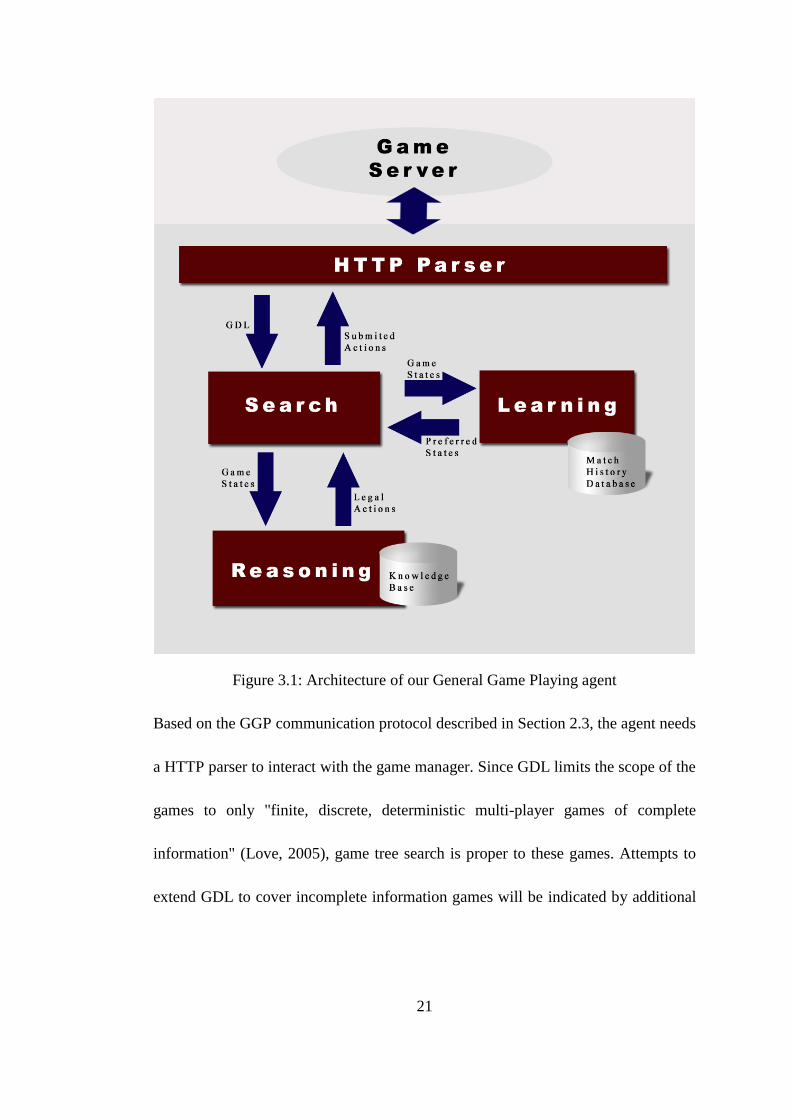
Figure 3.1: Architecture of our General Game Playing agent

Based on the GGP communication protocol described in Section 2.3, the agent needs

a HTTP parser to interact with the game manager. Since GDL limits the scope of the

games to only "finite, discrete, deterministic multi-player games of complete

information" (Love, 2005), game tree search is proper to these games. Attempts to

extend GDL to cover incomplete information games will be indicated by additional

22

keywords. We also need a reasoning module to identify legal actions in a given game

state and a learning module to evaluate the outcome of the actions. Our agent

architecture is shown in Figure 3.1. We'll explain each module in the following

sections of this chapter.

3.1 Heuristic Search

A complete game tree is a directed graph with the initial game state as the root, the

terminal states as the leaves, and all possible moves from each position as

intermediate tree nodes. The number of nodes in a complete game tree is bounded by

O(bd), where b is the branching factor and d is the game depth. Chess has roughly 38

84

(~10130

) possible game states (De Groot, 1965). Tic-Tac-Toe has roughly 39 (nine

cells, each with three possible values, ~19,000) possible intermediate game states.

Although a complete game tree can provide the optimal action at every step, in most

cases, it is too expensive to build.

In this dissertation, the term game tree refers to the partial game tree that uses the

current game state as the root and includes as many nodes as the player can search.

Search algorithms that explore one ply, two plies, ahead of the current state are called

one-step search, two-step search, respectively.

23

Assuming both players play optimally, minimax search can be used in two-player

complete information games. It recursively computes the minimax values of the

successor states, beginning from the tree leaves and backing up through the tree as the

recursion unwinds. Minimax is a depth first tree search. It has the space complexity of

O(bd) and time complexity of O(bd).

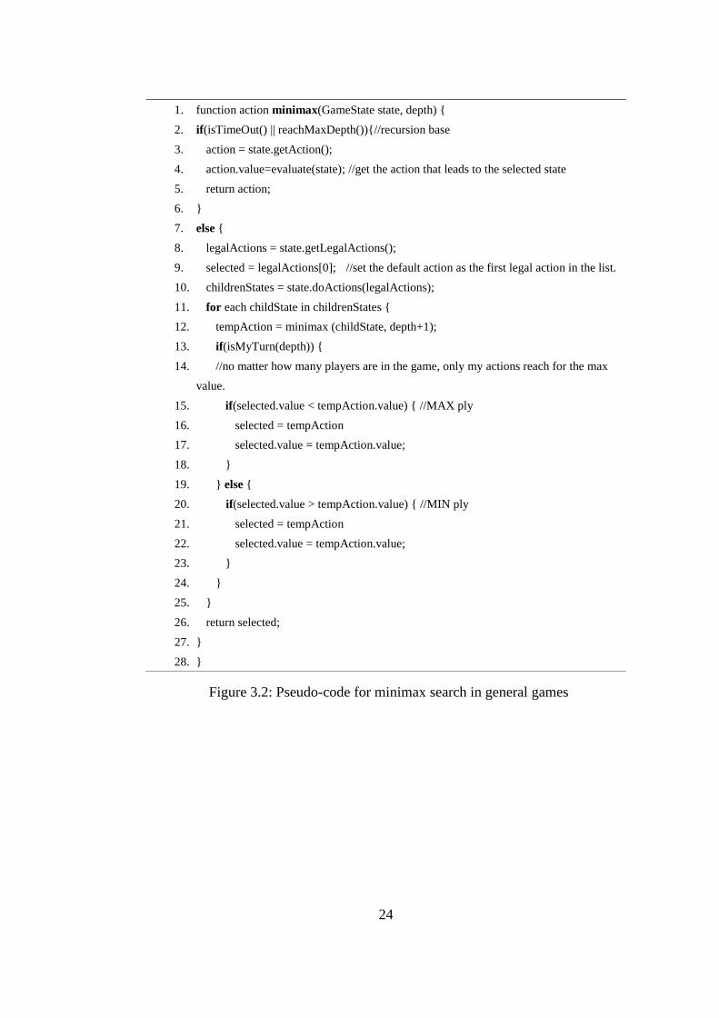
We make certain adjustments for the minimax search in our agent. For single-player

and simultaneous games, every ply is a MAX ply. For games with more than two

players, we assume each player is in competition with all others and attempts to make

optimal moves for himself. Therefore, all other players' moves are treated as MIN ply.

The minimax search becomes the max-min-min search in a three-player turn-taking

game.

Search algorithms used in GGP include Binary Decision Diagrams (Edelkamp, 2011),

Monte-Carlo Tree Search (Finnsson, 2011; Gudmundsson, 2011; Möller, 2011), and

tree parallelization (Méhat, 2011). Among these search algorithms, Monte-Carlo Tree

Search has recently been recognized as the new benchmark for game tree search in the

AI area (Kroeker, 2011). We are aware that minimax is not optimal in our algorithm

and should be replaced, but the focus of our research has been on the learning

algorithms as opposed to the search.

24

Figure 3.2: Pseudo-code for minimax search in general games

1. function action minimax(GameState state, depth) {

2. if(isTimeOut() || reachMaxDepth()){//recursion base

3. action = state.getAction();

4. action.value=evaluate(state); //get the action that leads to the selected state

5. return action;

6. }

7. else {

8. legalActions = state.getLegalActions();

9. selected = legalActions[0]; //set the default action as the first legal action in the list.

10. childrenStates = state.doActions(legalActions);

11. for each childState in childrenStates {

12. tempAction = minimax (childState, depth+1);

13. if(isMyTurn(depth)) {

14. //no matter how many players are in the game, only my actions reach for the max

value.

15. if(selected.value < tempAction.value) { //MAX ply

16. selected = tempAction

17. selected.value = tempAction.value;

18. }

19. } else {

20. if(selected.value > tempAction.value) { //MIN ply

21. selected = tempAction

22. selected.value = tempAction.value;

23. }

24. }

25. }

26. return selected;

27. }

28. }

25

3.2 Logic Resolution

A GGP game starts from one initial state and transits from one state to the next only

by actions. The agent uses the reasoning module to retrieve game states, each player's

roles, game transitions, game termination validation, and legal actions. Knowledge

representation and reasoning algorithms including inference, deduction, substitution

and unification are used in the agent (see Section 4.1).

Our first attempt to develop a learning algorithm used forward chaining to calculate

the legal actions in a given game state. The forward chaining approach starts from the

facts in the Knowledge Base (KB) and keeps solving the rules and adding new facts

entailed by the KB. This is supposed to be efficient because each time we mark a new

proposition as true, it will be added to the KB and can be re-used by another reasoning

thread without being re-generated. Since there are many propositions (e.g. board

adjacency) that stay unchanged from the beginning to the end of the game, calculating

them once and using them repeatedly should save time.

This assumption turned out to be wrong. As more and more propositions are added to

the KB, the size of the KB grew tremendously. The KB starts with only propositions

describing the game state and grows into millions of logical inferences that can be

generated from the KB about the game. Although the forward chaining procedure's

computational complexity can be reduced to linear in the size of the KB, the agent

26

needs to access the KB so frequently that trivial delays in the KB access can

significantly impair agent performance (see Section 4.2).

We had to revert to the backward chaining reasoning algorithm. It starts from the

target clause and works backward to the facts in the KB. The backward chaining itself

is not as efficient as forward chaining because it conducts a considerable amount of

redundant searching (Brachman, 2004). Yet it is more proper in the GGP context

because the KB size is kept small and the KB access is kept efficient.

3.3 Learning

While logic resolution is straight forward in determining the available legal actions,

selecting good actions remains challenging. Most games are too large to be searched

exhaustively so the search has to be truncated before a terminal state is reached. The

agent has to make decisions without perfect information. Evaluation functions replace

terminal or goal states so that the game can move forward.

Note that the evaluation functions return an estimate of the expected utility of the

game at a given state. The "guessing" is not as correct as searching but it can be very

useful. Research has shown that in a Chess game, even expert players seldom look at

more than 100 possible situations to decide on an action (De Groot, 1965). Compared

to Deep Blue that evaluates 200,000,000 states per second, humans excel with

27

intelligence and Deep Blue excels with computational power. The performance of a

game-playing program is dependent concurrently on its ability to search and the

quality of the evaluation. Our research focus is primarily on the quality of the

evaluation functions.

The purpose of general game playing is to build automated agents to play arbitrary

games. Learning is the core research problem in the GGP. It is indeed surprising that

the general learning algorithms have not dominated the state of the art in GGP. The

reason is mainly due to the difficulty of designing general-purpose learning

algorithms. The GGP competition set-up also makes it hard to differentiate how much

search or learning individually contributes to the agent's winning. Lack of evaluation

benchmarks has made it hard to measure the learning results (see Section 9.3). Three

known learning algorithms in GGP include transfer learning, temporal difference

learning, and neural network algorithms.

Transfer learning generalizes known games into directed graphs and uses graph

isomorphism to map the known strategies to new games (Kuhlmann, 2007; Banerjee,

2007). It is dependent on the availability of known games. When given a game that the

world has never seen before, the agent loses its advantage.

Game Independent Feature Learning (GIFL) is the temporal difference learning (Kirci,

2011), but is very much limited to two-player, turn-taking games. The features can be

28

learned only if the player that wins the game makes the last move. Features-to-Action

Sampling Technique (FAST) is another temporal difference method that uses

template matching to identify piece types and cell attributes (Finnsson, 2010). It is

designed to play board games only.

The neural network algorithm transforms the goal of a game to obtain an evaluation

function for states of the game (Michulke, 2009, 2011). It is capable of learning and

consequently, improving with experience. But games where the ground-instantiation

of the goal condition is not available, such as when the goal conditions (or predecessor

conditions in the chain) are defined in a recursive manner, are out of the scope of this

algorithm.

The learning algorithm we decided to pursue does not depend on any known games,

any game types, or assumptions of the game rules. It is based on game simulations,

not on how the game rules are written. Our learning algorithm has three steps. First,

the agent singles out influential features that helped the players win (see Chapter 5).

Second, the agent identifies some individual features that are more beneficial when

combined with certain other features. It uses a decision tree (see Section 6.2) to

evaluate the entire game state, not the individual features. Third, the agent moves

from global learning to local learning (see Section 6.3). The game states are better

differentiated when limited by the search bound.

29

3.4 Game Examples

We now give a few example games that we use in the rest of the dissertation to

illustrate the effectiveness and performance of the algorithms in building an

intelligent general game player. The games we chose include small, middle, and large

size games; single-player, two-player, and three-player games; zero-sum and

non-zero-sum games; turn-taking and simultaneous games; direct search, strategic

and eCommerce games.

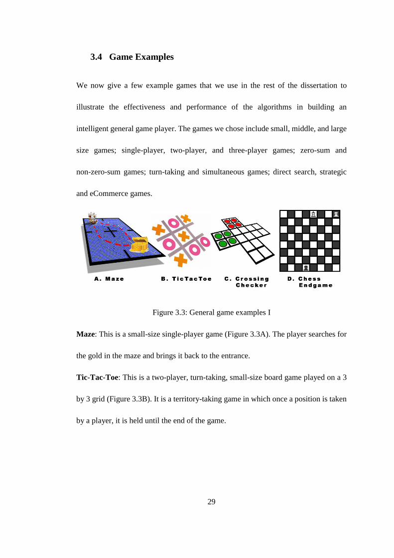
Figure 3.3: General game examples I

Maze: This is a small-size single-player game (Figure 3.3A). The player searches for

the gold in the maze and brings it back to the entrance.

Tic-Tac-Toe: This is a two-player, turn-taking, small-size board game played on a 3

by 3 grid (Figure 3.3B). It is a territory-taking game in which once a position is taken

by a player, it is held until the end of the game.

30

Crossing Chinese Checkers: Two players alternatively move or jump pieces to the

other end of the board (Figure 3.3C). Players can either move one grid forward or

jump over one piece and land on the other side. Players can repeat jumping until no

legal jump is available as part of the same move. The first player with all four pieces

in the target area wins.

Chess Endgame: This is a middle-size strategic game with three pieces left on the 8

by 8 Chess board (Figure 3.3D). The piece movements obey the regular Chess rules.

White needs to checkmate Black in at most 16 steps to win. Unlike Tic-Tac-Toe,

positions taken by players can be released.

Mini-Chess: Two players play on a 4 by 4 Chess board with the same movement rules

as regular Chess (Figure 3.4A). White has a rook at (c,1), and a king at (d,1). Black

has only a king at (a,4). This is an asymmetric game. White must checkmate Black in

at most ten steps; otherwise, Black wins.

Connect Four: Classic vertical Connect Four is a middle-size territory-taking game.

Two players alternatively drop pieces down slots from the top of a six by seven grid

(Figure 3.4B). The first player that connects four pieces in a line (horizontal, vertical,

or diagonal) wins. White goes first and it is advantageous to go first. Connect Four has

a branching factor of seven and the search space is roughly 342

.

31

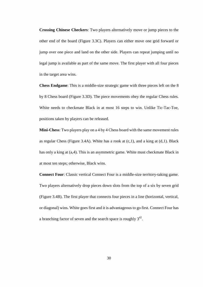
Figure 3.4: General game examples II

Othello: Othello is a large-size two-player territory-taking game (Figure 3.4C). The

player tries to flip the opponent's pieces into his own color. The player with majority

of pieces showing at the end of the game wins. Othello has a branching factor of 8-12

and a search space of roughly 364

(~1030

) .

Farmer: Farmer is a three-player simultaneous game especially written for GGP

(Figure 3.4D). Traditional computer game research covers mainly two-player

turn-taking games, but the Farmer game sets up tasks for three players (Alice, Barney

and Charlie) to make as much money as possible in the given iterations. Each player

tries to make more money than either of the other players. In each iteration, all three

players act simultaneously.

The three players each start with 25 gold pieces. It takes 10 gold pieces to build (buy)

a farm and 20 gold pieces to build a factory. The players begin with no commodities

on hand. They have to build a farm before growing wheat or cotton and build a factory

before making flour or cloth out of their existing wheat or cotton inventory. Once the

32

farm is built it will produce wheat if the “grow wheat” action is taken or cotton if the

“grow cotton” action is taken at any subsequent iteration. Once the factory is built it

will produce flour if the “manufacture flour” action is taken or cloth if the

“manufacture cloth” action is taken, provided the player has the required wheat or

cotton in inventory.

However, manufacturing products from raw materials is not the only way to make

money. Players can buy and sell directly to the market as well. The market has an

infinite supply of commodities and gold. The initial market price for wheat is 4 gold

pieces, flour 10, cotton 7 and cloth 14 gold pieces. After every step of the game, the

market price of each commodity automatically increases by one even if nothing is

bought or sold. In addition to this automatic increase, the product price decreases by

two in the next iteration for every selling action of that commodity and increases by

two in the next iteration for every buying action of that commodity. The players begin

with no inventory. The buy action will fill up the player’s inventory with that

commodity and the sell action will clear the inventory of that commodity. Essentially

all commodities except gold have only a single unit size.

The Farmer game is a very interesting game in many aspects. It contains a simplified

skeleton of manufacturer financial activities, such as invest in infrastructure (farm or

factory), buying raw material from the market, selling the product to the market, and

33

keeping the inventory down. It also contains the elements of the stock market, such as

an inflation indicator (prices increase by one in every step) and a market pressure

indicator (price goes down by two for every selling action, and up by two for every

buying action). The Farmer game opens the possibility of using general game playing

techniques to explore, and perhaps even solve, skeletal real world financial or social

problems.

Another outstanding feature about the Farmer game is the simultaneous movement of

all three players. Each player can buy or sell one of the four commodities, grow or

make one of the four raw materials, or build one of the two infrastructures. Each

player has 12 to 14 possible legal actions in every step. In other words, the branching

factor is about 123 because the three players move simultaneously. The typical

branching factors is 36 for Chess, 7 for Connect Four, 10 for Checkers, and 300 for Go

--- all are well-recognized complex games. The complexity of the Farmer game is

amazing.

The Farmer game can be very flexible too. The game can be easily reconfigured from

three players to two, four or more players. It can be changed from 10 iterations to 20,

40 or more iterations. The game dynamics change accordingly. Further discussions on

the Farmer game can be found in Sections 5.4, 6.2.4, and 7.4.

34

4 Knowledge Representation and Reasoning

As mentioned in Chapter 2, the game manager provides the player agents with the

initial state of the game, the set of game rules, and their roles in the game. The game

state information is in the form of logic propositions. The game's legal actions and

goals are defined in the form of logic relations. The agents' roles in the game are

provided in the form of logic statements. With such information, the agents use

knowledge representation and reasoning to calculate the available actions. It is

impossible to conduct further game operations such as game tree search or learning

without knowledge resolution. Reasoning is the foundation in all general game

players. However, not all reasoning algorithms are the same. The contents in this

chapter have been published (Sheng, 2010b).

4.1 Reasoning with Logic: Substitution, Unification and

Backward Chaining

The game state is a collection of true propositions or facts. The facts are stored in the

Knowledge Base (KB). The game rules are written in prefix logic implications.

Reasoning is the process of using the implications from the existing propositions to

35

produce a new set of propositions. The reasoning algorithms used in our general game

player include substitution, unification and backward chaining.

We now use Tic-Tac-Toe game as an example. Suppose the grid is marked as in

Figure 4.1 and O-player is in control in the current state. The game relation row is

defined as below:

(<= (row ?x ?player)

(true (cell ?x 1 ?player))

(true (cell ?x 2 ?player))

(true (cell ?x 3 ?player)))

Figure 4.1: Tic-Tac-Toe example

The arguments that begin with ? are variables. To answer the question "Is there an ?x

value such that (cell ?x 1 ?player) is true?", the inference rule substitution is used.

Substitution inference is looking for a variable/ground term pair so that the

proposition sentence is true (Russell, 2003). In the Figure 4.1 example, (cell 1 1 X)

and (cell 3 1 O) are both true propositions coming out of the inference.

36

The substitution rule gives different groups of variable assignments to each condition

in the row implication. For the first condition clause (true (cell ?x 1 ?player)), the

assignments are {x=3, player =O}, {x=1, player =X}. For the second clause (true

(cell ?x 2 ?player)), the assignments are {x=1, player =X}. The unification rule is

introduced to combine the two clauses. Unification requires finding substitutions to

make different logic expressions identical (Russell, 2003). Only the pair {x=1, player

=X} satisfies both the first condition and the second condition concurrently.

Using the unification inference recursively until all clauses in the implication body are

unified with a known fact is the process called backward chaining. Backward

chaining is the goal-oriented reasoning that finds implications in the knowledge base

that conclude with the goal (Russell, 2003). If the clause cannot be determined in the

current implication, the agent introduces other rules to the process.

4.2 Limitations of the Knowledge Base

In the reasoning process, the propositions are stored in the KB. When the game state

proceeds forward or a new query is needed, the agent searches the KB to substitute

variable values with grounded terms. New propositions will be generated, and copied

into the KB to store.

37

Tic-Tac-Toe is a simple example and we use it only for illustration purposes. Connect

Four is a middle-size game with a branching factor of seven. Othello is a large-size

game with a branching factor that varies from 8 to 12. The KB is very frequently

queried for both proposition search (returning all applicable values) and theorem

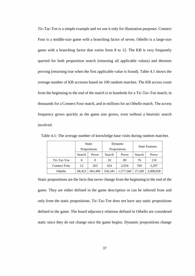
proving (returning true when the first applicable value is found). Table 4.1 shows the

average number of KB accesses based on 100 random matches. The KB access count

from the beginning to the end of the match is in hundreds for a Tic-Tac-Toe match, in

thousands for a Connect Four match, and in millions for an Othello match. The access

frequency grows quickly as the game size grows, even without a heuristic search

involved.

Table 4.1: The average number of knowledge base visits during random matches

Static

Propositions

Dynamic

Propositions State Features

Search Prove Search Prove Search Prove

Tic-Tac-Toe 0 0 10 80 76 110

Connect Four 12 263 424 2,016 760 3,297

Othello 68,423 603,490 556,345 1,577,560 27,269 2,008,058

Static propositions are the facts that never change from the beginning to the end of the

game. They are either defined in the game description or can be inferred from and

only from the static propositions. Tic-Tac-Toe does not have any static propositions

defined in the game. The board adjacency relations defined in Othello are considered

static since they do not change once the game begins. Dynamic propositions change

38

over the game cycle. They can be added or removed as the game proceeds. State

features contain the game state information and are the most frequently queried group

of the three.

The KB is accessed frequently during the game cycle. So the data structure in the KB

affects the reasoning performance of the agent. The larger the game, the more

significant the influences of the KB data structure are. A small performance

improvement in the reasoning process can be greatly amplified to expedite searches

and learning and therefore, add up to huge improvements in the agent's performances.

GDL has been known as not particularly efficient in reasoning, and there are many

attempts to improve its performance (see Section 2.4).

4.3 Using Hash Tables to Expedite Reasoning

We propose using hash tables to improve the reasoning performance. Hash tables use

hash functions to convert data into indexed array elements. A hash table is a

commonly used data structure to improve the search performance. Depending on the

implementation, the searching complexity varies, but the time complexity of

searching a hash table can be as low as O(1). We designed the hash function so that it

groups all propositions starting with the same logic terms together. Because the

number of logic relation terms is very limited (as in the game playing context), the

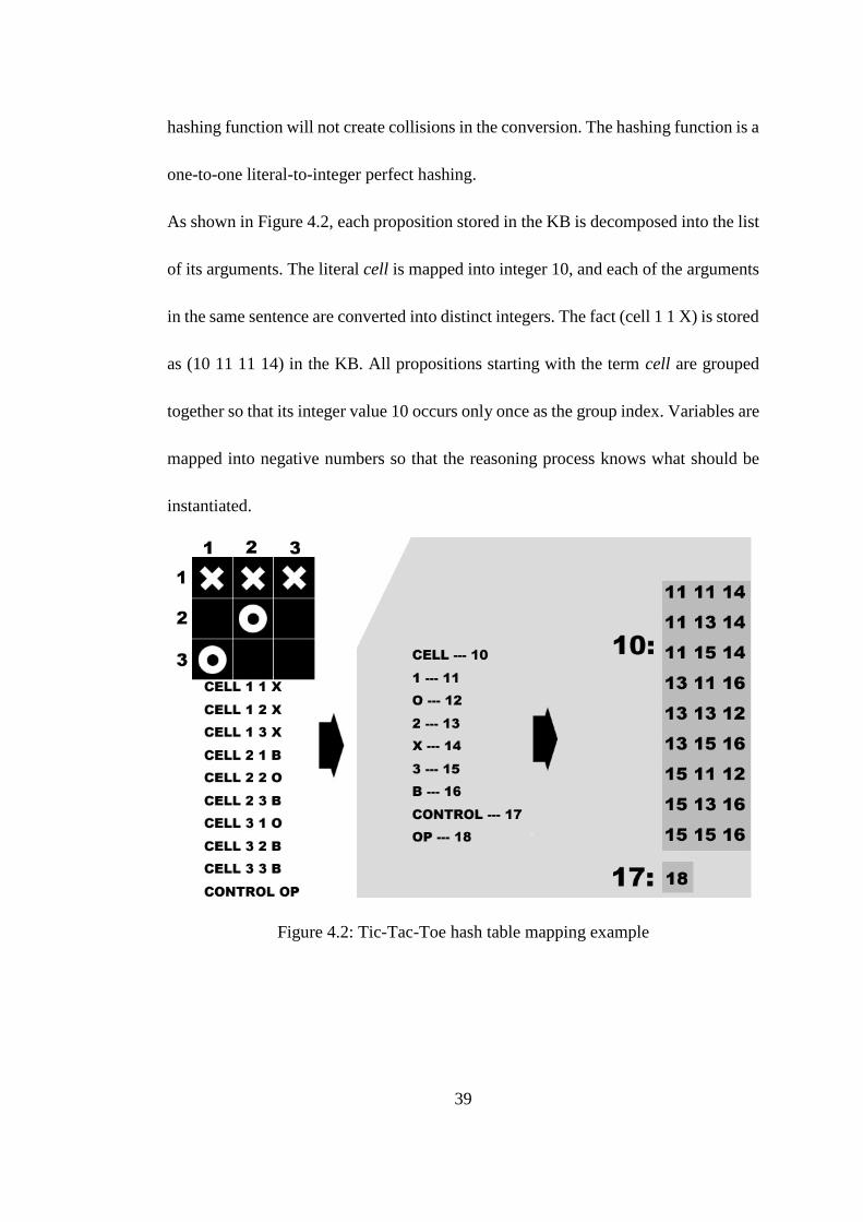
39

hashing function will not create collisions in the conversion. The hashing function is a

one-to-one literal-to-integer perfect hashing.

As shown in Figure 4.2, each proposition stored in the KB is decomposed into the list

of its arguments. The literal cell is mapped into integer 10, and each of the arguments

in the same sentence are converted into distinct integers. The fact (cell 1 1 X) is stored

as (10 11 11 14) in the KB. All propositions starting with the term cell are grouped

together so that its integer value 10 occurs only once as the group index. Variables are

mapped into negative numbers so that the reasoning process knows what should be

instantiated.

Figure 4.2: Tic-Tac-Toe hash table mapping example

40

Using hash tables to convert the data stored in KB from game specific features to

integers not only saves storage space, but also saves search time. Without hashing, the

KB search conducts string comparisons and is dependent on the length of the string.

Suppose one proposition has an average of n strings, and each string has an average of

m letters. A positive equal comparison has the computational complexity of O(m*n).

But using the hash table, only O(n) comparisons are needed. The length of the string

does not matter anymore. The savings are beneficial to any GGP player that uses logic

substitution, unification and backward chaining reasoning algorithms.

Some GGP players in the field choose to convert GDL into other programming

languages with better AI support, such as Prolog or LISP, or other compilers or

reasoning tools. The hash tables presented here create a one-to-one hashing schema

that map each game element into a unique integer. The agent does not need to handle

hashing value collisions. Perfect hashing is as good as any hashing method can do.

The hash table is of the same cardinality as the game rules.

To avoid human cheating, all the competition games are scrambled into random letter

combinations, which can be long, meaningless strings. For example, (cell 1 1 B),

which means a ternary relation cell that relates a row number, a column number, and a

content designator, is logically equivalent to the description (position first first empty),

or scrambled version (tsrtysdfmpzz ryprry ryprry fmajafgh), as long as the terms are

41

replaced consistently for all other occurrences in the game rules. With the proposed

hash tables, as long as the logic relations are the same, the scrambled version of the

game will be treated the same, no matter if the logic relation is scrambled into

two-letter words or two-hundred-letter words.

In addition to converting the data stored in the KB, we expand the hash values to the

reasoning process. When the agent receives the game description at the beginning of

the game, it converts the entire game logic into integers. Which literal is used does not

affect the logic relations as long as the changes are consistent. Therefore, the rule (<=

(goal ?player 100) (line ?player)) is logically equivalent to (<= (15 -3 77) (26 -3)) as

long as the terms are changed consistently for other places in the game rules. Figure

4.2 shows how the propositions in the Tic-Tac-Toe example game state are converted

into distinct integers in the KB. The pseudo-code for hashing the game description

written in GDL to integers is presented as in Figure 4.3.

The standard Java API is used in the calculation. The hash code of a string is

calculated from the ASCII value of each letter in the string, as shown in function

hashCode. To avoid collisions, the hash code is mapped into a unique index value

with the getIndex function, creating a perfect hash. In general game playing

circumstances, even for a very complicated game like Chess or Othello, the rules in

GDL are only a few pages. Therefore, the number of literals used in one game

42

description is limited, possibly less than one hundred. We have not seen any actual

hash collisions in all known GGP example games (list given in Appendix A). Perfect

hashing of game literals creates a table of the same cardinality as the game description

and does not require a heavy maintenance burden.

43

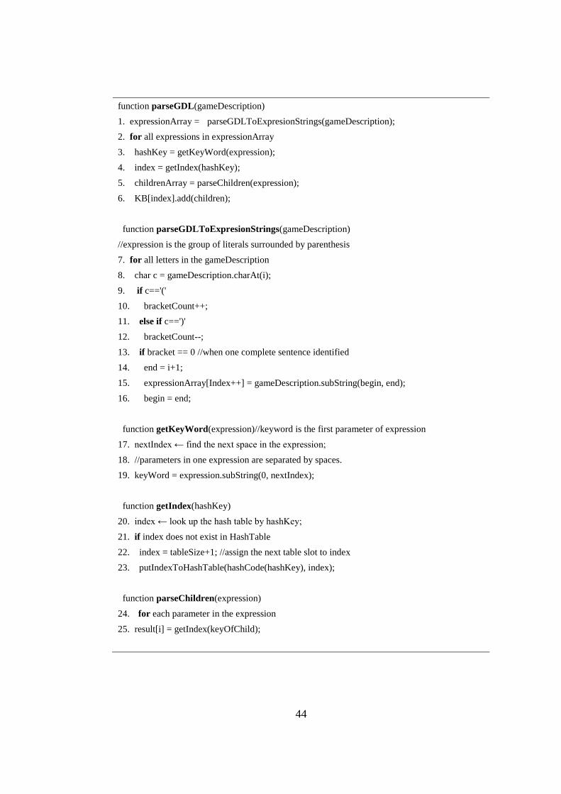
Figure 4.3: Pseudo-code for converting GDL sentences into hash tables

44

function parseGDL(gameDescription)

1. expressionArray = parseGDLToExpresionStrings(gameDescription);

2. for all expressions in expressionArray

3. hashKey = getKeyWord(expression);

4. index = getIndex(hashKey);

5. childrenArray = parseChildren(expression);

6. KB[index].add(children);

function parseGDLToExpresionStrings(gameDescription)

//expression is the group of literals surrounded by parenthesis

7. for all letters in the gameDescription

8. char c = gameDescription.charAt(i);

9. if c=='('

10. bracketCount++;

11. else if c==')'

12. bracketCount--;

13. if bracket == 0 //when one complete sentence identified

14. end = i+1;

15. expressionArray[Index++] = gameDescription.subString(begin, end);

16. begin = end;

function getKeyWord(expression)//keyword is the first parameter of expression

17. nextIndex ← find the next space in the expression;

18. //parameters in one expression are separated by spaces.

19. keyWord = expression.subString(0, nextIndex);

function getIndex(hashKey)

20. index ← look up the hash table by hashKey;

21. if index does not exist in HashTable

22. index = tableSize+1; //assign the next table slot to index

23. putIndexToHashTable(hashCode(hashKey), index);

function parseChildren(expression)

24. for each parameter in the expression

25. result[i] = getIndex(keyOfChild);

45

function hashCode(hashKey) // standard Java String.hashcode() API

26. if the hashKey is empty

27. hashcode = 0;

28. else

29. for each letter in the hashKey

30. hashCode = hashKey.charAt[i] + ((hashCode << 5) - hashCode);

46

In our agent, the knowledge representation and reasoning process are conducted with

integers. Only the equal and not-equal operations are invoked. No addition or

subtraction operations are allowed. The hashing conversion from GDL to the integers

is processed only once at the beginning of the game. Subsequent reasoning is

conducted directly with integers and access only the KB but do not search the hash

table key-value pairs. Introducing hash tables into the reasoning process is because

the KB is visited extremely often (Table 4.1). When communicating to the game

manager, the agent translates the integers back into the strings. Considering the

communication is only done at the end of each step, this translation cost is minimal.

4.4 Hash Tables Performance Analysis

Dresden University of Technology general game playing website has published a Java

agent player (see reference GGP Player). Our GGP agent is written in Java and we

compare our agent against the published Java agent for performance benchmarks.

Different games have different logic relations and therefore different reasoning

computational complexities. We compare our agent and the published Dresden Java

agent in seven games: Maze, Mini-Chess, Tic-Tac-Toe, Connect Four, Chess

Endgame, Othello, and Farmer. A wide variety of different game sizes, player

numbers, and dynamics are covered.

47

The experiments were run on a desktop PC with Intel Q6600 2.4GHz CPU, 2GB

memory, and Ubuntu Linux 10.04. To design a fair comparison to test the reasoning

speed of the two Java players, we used three criteria:

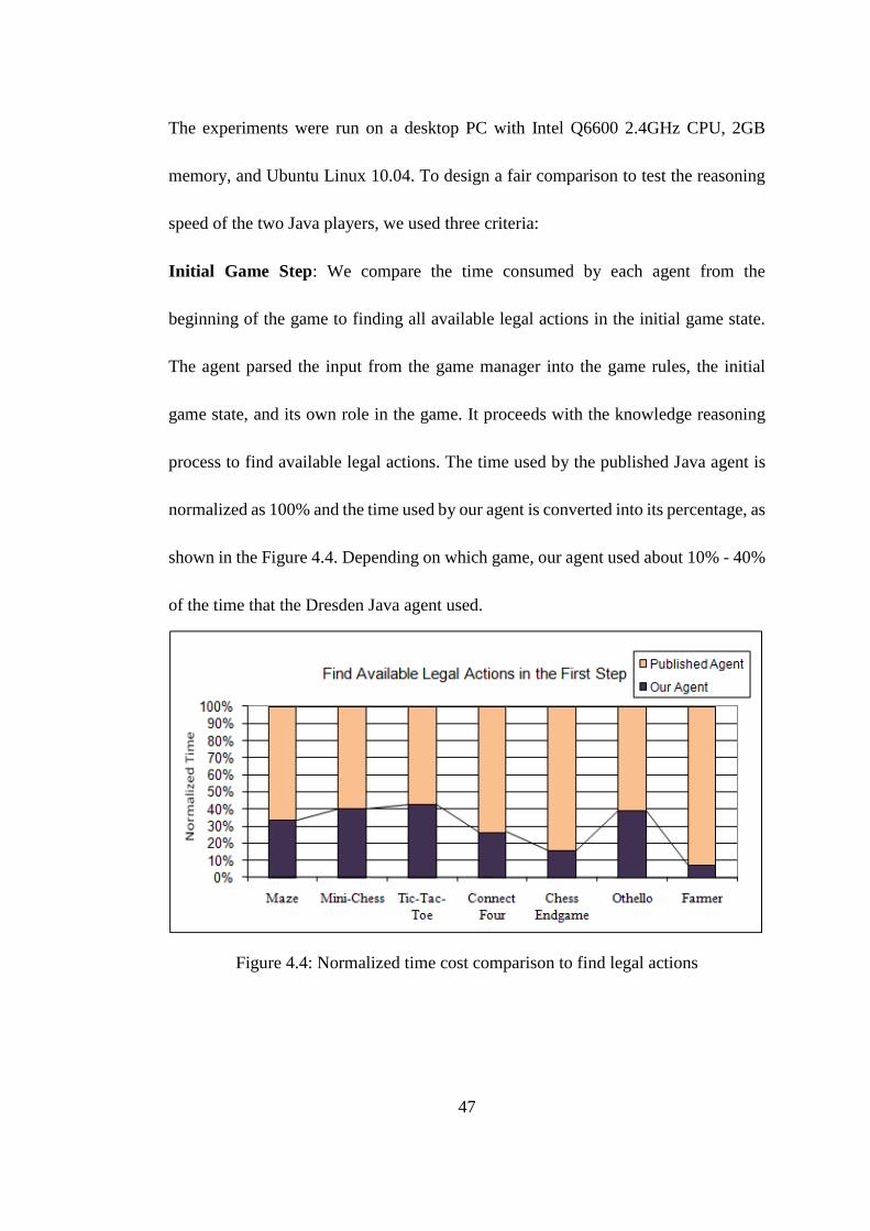
Initial Game Step: We compare the time consumed by each agent from the

beginning of the game to finding all available legal actions in the initial game state.

The agent parsed the input from the game manager into the game rules, the initial

game state, and its own role in the game. It proceeds with the knowledge reasoning

process to find available legal actions. The time used by the published Java agent is

normalized as 100% and the time used by our agent is converted into its percentage, as

shown in the Figure 4.4. Depending on which game, our agent used about 10% - 40%

of the time that the Dresden Java agent used.

Figure 4.4: Normalized time cost comparison to find legal actions

48

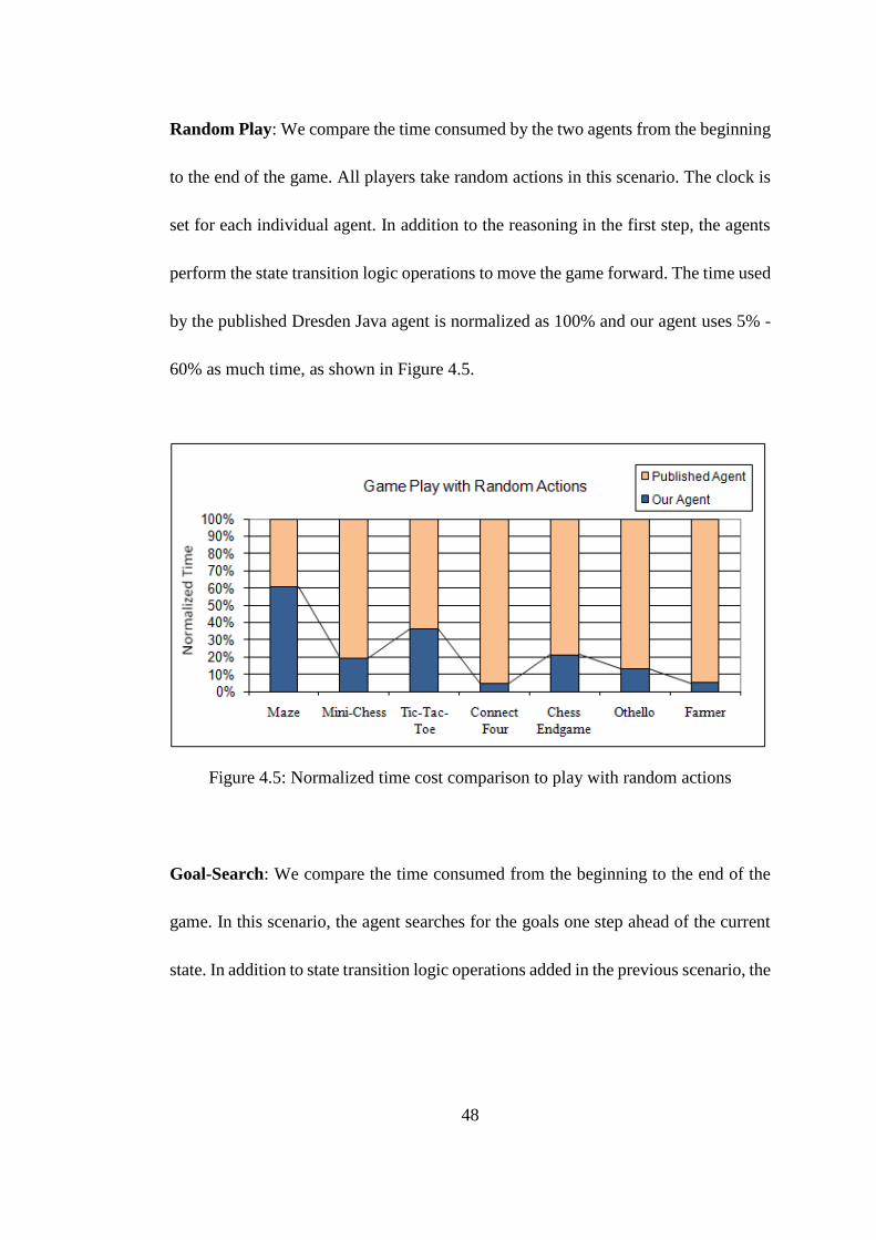
Random Play: We compare the time consumed by the two agents from the beginning

to the end of the game. All players take random actions in this scenario. The clock is

set for each individual agent. In addition to the reasoning in the first step, the agents

perform the state transition logic operations to move the game forward. The time used

by the published Dresden Java agent is normalized as 100% and our agent uses 5% -

60% as much time, as shown in Figure 4.5.

Figure 4.5: Normalized time cost comparison to play with random actions

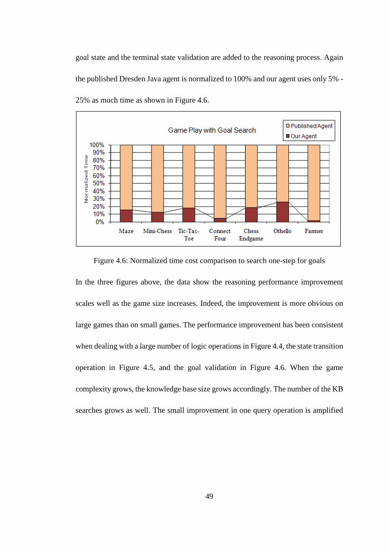
Goal-Search: We compare the time consumed from the beginning to the end of the

game. In this scenario, the agent searches for the goals one step ahead of the current

state. In addition to state transition logic operations added in the previous scenario, the

49

goal state and the terminal state validation are added to the reasoning process. Again

the published Dresden Java agent is normalized to 100% and our agent uses only 5% -

25% as much time as shown in Figure 4.6.

Figure 4.6: Normalized time cost comparison to search one-step for goals

In the three figures above, the data show the reasoning performance improvement

scales well as the game size increases. Indeed, the improvement is more obvious on

large games than on small games. The performance improvement has been consistent

when dealing with a large number of logic operations in Figure 4.4, the state transition

operation in Figure 4.5, and the goal validation in Figure 4.6. When the game

complexity grows, the knowledge base size grows accordingly. The number of the KB

searches grows as well. The small improvement in one query operation is amplified

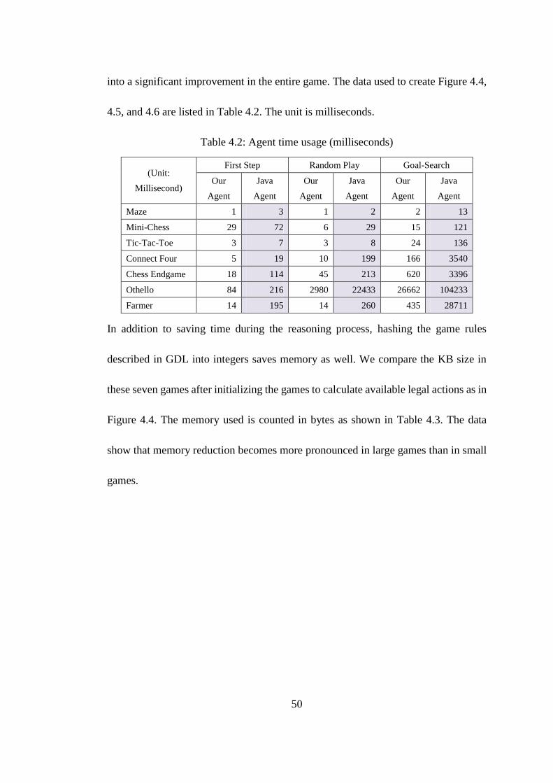
50

into a significant improvement in the entire game. The data used to create Figure 4.4,

4.5, and 4.6 are listed in Table 4.2. The unit is milliseconds.

Table 4.2: Agent time usage (milliseconds)

(Unit:

Millisecond)

First Step Random Play Goal-Search

Our

Agent

Java

Agent

Our

Agent

Java

Agent

Our

Agent

Java

Agent

Maze 1 3 1 2 2 13

Mini-Chess 29 72 6 29 15 121

Tic-Tac-Toe 3 7 3 8 24 136

Connect Four 5 19 10 199 166 3540

Chess Endgame 18 114 45 213 620 3396

Othello 84 216 2980 22433 26662 104233

Farmer 14 195 14 260 435 28711

In addition to saving time during the reasoning process, hashing the game rules

described in GDL into integers saves memory as well. We compare the KB size in

these seven games after initializing the games to calculate available legal actions as in

Figure 4.4. The memory used is counted in bytes as shown in Table 4.3. The data

show that memory reduction becomes more pronounced in large games than in small

games.

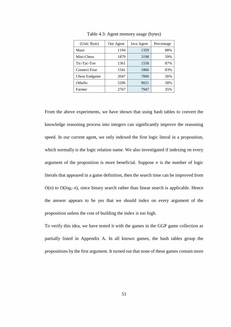
51

Table 4.3: Agent memory usage (bytes)

(Unit: Byte) Our Agent Java Agent Percentage

Maze 1194 1359 88%

Mini-Chess 1879 3198 59%

Tic-Tac-Toe 1361 1558 87%

Connect Four 1541 1866 83%

Chess Endgame 2047 7860 26%

Othello 5206 9021 58%

Farmer 2767 7947 35%

From the above experiments, we have shown that using hash tables to convert the

knowledge reasoning process into integers can significantly improve the reasoning

speed. In our current agent, we only indexed the first logic literal in a proposition,

which normally is the logic relation name. We also investigated if indexing on every

argument of the proposition is more beneficial. Suppose n is the number of logic

literals that appeared in a game definition, then the search time can be improved from

O(n) to O(log2 n), since binary search rather than linear search is applicable. Hence

the answer appears to be yes that we should index on every argument of the

proposition unless the cost of building the index is too high.

To verify this idea, we have tested it with the games in the GGP game collection as

partially listed in Appendix A. In all known games, the hash tables group the

propositions by the first argument. It turned out that none of these games contain more

52

than 100 game relations. So the problem size n is less than 100. The cost of search is

close to the cost of building the index on each argument.

To summarize, in the general game playing field, knowledge representation and

reasoning are the fundamental operations for the agent to understand and participate

in the game. Although the logic inference algorithms have been available for a long

time, how to implement them for the agents' performances when dealing with

computational intensive tasks remains a challenge. A small performance

improvement in the reasoning process can be greatly amplified to expedite searches

and learning, and thus potentially add up to huge improvements in agents'

performances. We have shown in seven heterogonous games that our hash tables can

save significant computation time and memory in the reasoning process.

53

5 Sub-Goal Identification

Given a completely new game, the GGP agent uses knowledge representation and

reasoning algorithms to calculate legal actions. To decide which action to take, the

agent uses machine learning algorithms to discover which are beneficial for winning.

This chapter connects the knowledge-based game states with the simulation-based

game process. We present a feature identification algorithm that analyzes winning

features to quantify how much certain features predict the winning. These important

winning features are treated as temporary goals in the game and the agent actively

seeks them in the game tree search. The contents in this chapter have been published

(Sheng, 2010a).

5.1 Generating Training Set with Simulation

If an agent has unlimited time and space resources, it can build a complete game tree

and make optimal choices in every step. But most games are too large to be searched

exhaustively so the search has to be truncated before a goal state is reached. When the

game goals, as defined in the game rules, are out of the search range and are

non-deterministic, the agent has to make some decisions without perfect information.

This is why machine learning is used to help the agent.

54

Perhaps the first question in the learning process is: where can we get a good player

from which to learn? While a particular game playing program can learn from human

game experts or extensive opening and closing books, a general game playing agent

does not have that luxury but is expected to handle a game that the world has never

seen before.

5.1.1 Random Simulation versus Active Learning

We now introduce an automatic feature recognition algorithm that does not use any

assumptions about the games. The agent uses a self-play simulation database to record

the agent's past actions for analysis. One way to create the self-play database is by

running simulations of players using random decisions for any given game. Each

random match can be understood as one random path, from the initial game state to

the terminal game state in the game tree. Given enough simulations, these random

paths approximate the complete game tree in an evenly distributed manner. Another

possibility to create the simulation database is using active learning to run simulations

with learned agents and improve the agents as more simulations are available. The

two approaches have strengths and weaknesses. The former is unbiased but needs a

larger training set, while the latter loses the generality and decreases the coverage of

the game tree, but can be more efficient. We use the former to set up our training set

55

due primarily to better game tree coverage and a theoretically more conservative

approach.

When given a game to play, the agent plays and records its actions. The agent

generally does not win more than its "random share" in random playing, but the

random play does provide a chance for the agent to observe the game, explore the

game space and analyze the outcome of these actions. The agent will examine the

winners' history to see what elements, if any, the winners have in common. The

common winning elements can be the status of the board, the positions of the pieces,

the actions taken, the existence or absence of some features, etc. From the simulation

runs, the agent picks out the winners' history and identifies common features that

appeared to help the players win. Statistical analysis is used to decide how likely the

occurrence of a certain feature predicts winning. Features with high probabilities to

predict winning, called sub-goals, are singled out and are considered desirable in the

game tree search. The sub-goal identification approach is independent of specific

games. It is designed to fit games that can produce winners during random play. As

the game dynamics change, the identified features change automatically.

56

5.1.2 Determining the Simulation Size

The purpose of using machine learning is not because it is more accurate than the

complete game tree, but because it is more feasible. The simulation sacrifices the

accuracy of a complete game tree search in exchange for efficiency. Too few

simulations will not provide useful results, but too many simulations will be more

expensive than needed.

The learning process is expected to distinguish game elements that have a significant

positive influence on the game outcome. The sequential order of these game features

provides more utility than the absolute value of the features. The agent keeps track of

the statistical frequency of the features. The occurrence of certain game elements has

a probabilistic correlation with the outcome of the game. The features' occurrence

probabilities are used to determine if the features' sequential order has been

established at 95% confidence interval. If not, additional simulations are run (in

groups of 1000). We increase the number of simulation runs until we are certain the

sequential order has been established, or can never be established, for the game

features. Hypothesis testing is used to verify the utility order of the features when their

95% confidence intervals are disjoint.

57

5.1.3 Out of Scope Situations

The sub-goals identified from random simulations enable us to learn to play some

games that are not exhaustively searchable. However, the branching factor for some

games can be so large and the goals so deep that it is computationally too expensive to

reach the goal states by taking random actions. When not enough complete paths that

result in wins in the game tree are explored, the simulation set may not be big enough

to represent the game. Then it may be computationally impractical to obtain an

adequate sized learning set.

For games that are hard to win with random play (not necessarily with large branching

factors), efficiency weights over impartiality in training set generation. Without a

reasonable size training set, the learning module in the agent as designated in Figure

3.1 will be bypassed for not being able to provide beneficial suggestions on action

selection. The agent can still submit legal actions in the game play, but its

performance will be about the same as a goal-search player. Importing history from

external resources such as opening book and close book is a possible solution to get

the training set for the learning module. But it violates the expectation of generality

and that is beyond the scope of this dissertation.

58

5.2 Identify the Sub-Goals

Game feature is defined as the predicate naturally provided in the game description.

Depending on how a game is written, a game feature can have one dimension, such as

(control White), two dimensions, such as (distinct a b), three dimensions, such as (cell

x y blank), or more dimensions. We deal with the entire predicate as one unit because

it contributes as one entity in logic reasoning.

The agent encounters a large number of features from the beginning to the end of a

game. We are interested in only a very small subset that significantly helps win the

game. Using sub-goals identified from the previous playing history can guide the

heuristic game tree search when a exhaustive search is not feasible. Unlike the goals

defined in the game description with clear payoffs, the game sub-goals are not

self-evident.

The sub-goals have to be tested to see if they contribute to a winning strategy. For

example, in a turn-taking game like Tic-Tac-Toe, each player has control to take

actions half of the time. However, in all games that X-player won, X-player always

ended up in control. This is because when X-player forms a line to win the game, the

game ended without transferring the control to O-player. In this case, (control

X-player) is a frequently occurring feature shared by the winners but it is not

considered a sub-goal. Another example is the step counter in Mini-Chess (Figure

59

3.4A) and Chess Endgame (Figure 3.3D). These features are always present in the

winners' state. But their existence has no effect on winning. They are the simultaneous

occurrence of winning but not part of a winning strategy.

In addition to sub-goal identification, this algorithm can identify anti-goals, which are

features that would hurt the player. In other words, to win the game, the agent player

should actively avoid certain features. Depending on the game goal definition,

features to avoid have different meanings in different game contexts.

Numerical values are assigned to quantify the payoffs of the sub-goals. Note that

sub-goals are used only to guide the heuristic game tree search when the exhaustive

search is not feasible. Sub-goals are never as good as actual goals - they sacrifice the

accuracy of complete game tree search for efficiency. The sub-goals come out of

learning from simulation runs and are used to win future games. To test if high

occurrences features are actually sub-goals, we designed experiments in the next

section to test if using such features (values) to guide the search helps win.

5.3 Sub-Goal Analysis Example

We use Tic-Tac-Toe as an example to illustrate how sub-goals are identified. For a

human player, it is easily to tell that the middle position in Tic-Tac-Toe is the most

important, then the four corners, and finally the middle of the edges. But the game

60

agent does not know these priorities. The agent sees a completely new game with

rules defined in logic relations and it needs to figure out proper actions.

5.3.1 Statistical Analysis

The agent runs random matches repeatedly to simulate a proportional abstraction of

the game tree. The experiments used the pseudo-random seed 1234 to generate

random numbers and the constant coefficient 1.96 as the t-distribution critical value

for 95% confidence interval (Wackerly, 2008). The agent divides the simulation

results into 30 groups, with 100 matches in each group. These parameters are for

explanation only. If the readers choose to use other random seeds or match grouping

methods, the experiment results should be statistically equivalent.

For each feature, the agent adds up all of its occurrences in that group, then divides by

the number of games that X-player ended up winning in that group. It calculates the

95% confidence interval of the features' occurrence in the winners' end game. Figure

5.1 has the list of X-player’s preferred features based on 95% confidence interval,

ordered according to occurrence probability from high to low.

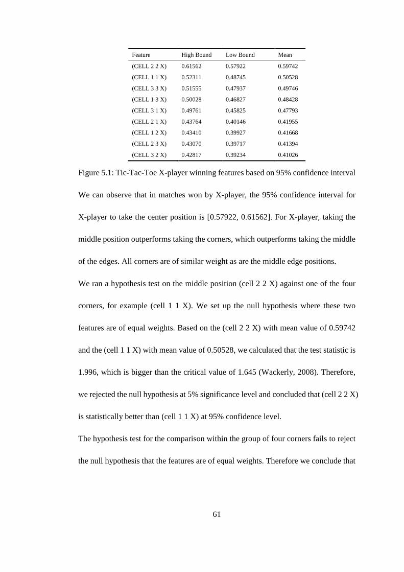
61

Feature High Bound Low Bound Mean

(CELL 2 2 X) 0.61562 0.57922 0.59742

(CELL 1 1 X) 0.52311 0.48745 0.50528

(CELL 3 3 X) 0.51555 0.47937 0.49746

(CELL 1 3 X) 0.50028 0.46827 0.48428

(CELL 3 1 X) 0.49761 0.45825 0.47793

(CELL 2 1 X) 0.43764 0.40146 0.41955

(CELL 1 2 X) 0.43410 0.39927 0.41668

(CELL 2 3 X) 0.43070 0.39717 0.41394

(CELL 3 2 X) 0.42817 0.39234 0.41026

Figure 5.1: Tic-Tac-Toe X-player winning features based on 95% confidence interval

We can observe that in matches won by X-player, the 95% confidence interval for

X-player to take the center position is [0.57922, 0.61562]. For X-player, taking the

middle position outperforms taking the corners, which outperforms taking the middle

of the edges. All corners are of similar weight as are the middle edge positions.

We ran a hypothesis test on the middle position (cell 2 2 X) against one of the four

corners, for example (cell 1 1 X). We set up the null hypothesis where these two

features are of equal weights. Based on the (cell 2 2 X) with mean value of 0.59742

and the (cell 1 1 X) with mean value of 0.50528, we calculated that the test statistic is

1.996, which is bigger than the critical value of 1.645 (Wackerly, 2008). Therefore,

we rejected the null hypothesis at 5% significance level and concluded that (cell 2 2 X)

is statistically better than (cell 1 1 X) at 95% confidence level.

The hypothesis test for the comparison within the group of four corners fails to reject

the null hypothesis that the features are of equal weights. Therefore we conclude that

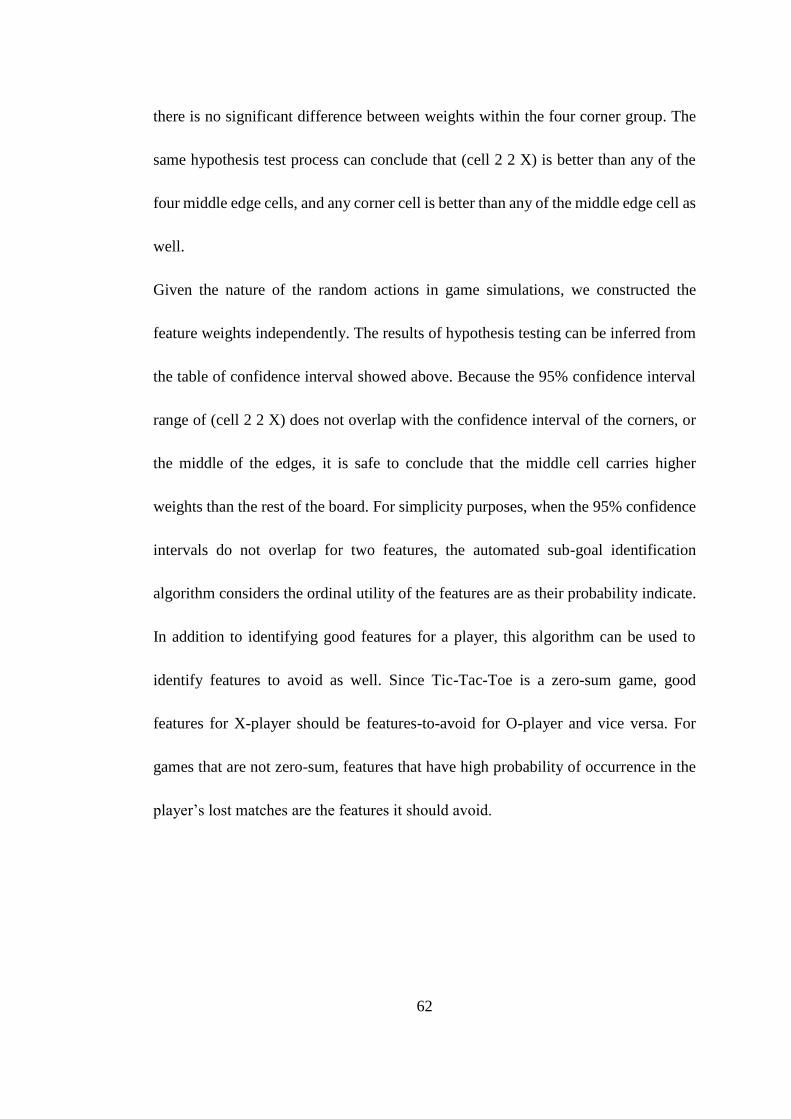
62

there is no significant difference between weights within the four corner group. The

same hypothesis test process can conclude that (cell 2 2 X) is better than any of the

four middle edge cells, and any corner cell is better than any of the middle edge cell as

well.

Given the nature of the random actions in game simulations, we constructed the

feature weights independently. The results of hypothesis testing can be inferred from

the table of confidence interval showed above. Because the 95% confidence interval

range of (cell 2 2 X) does not overlap with the confidence interval of the corners, or

the middle of the edges, it is safe to conclude that the middle cell carries higher

weights than the rest of the board. For simplicity purposes, when the 95% confidence

intervals do not overlap for two features, the automated sub-goal identification

algorithm considers the ordinal utility of the features are as their probability indicate.

In addition to identifying good features for a player, this algorithm can be used to

identify features to avoid as well. Since Tic-Tac-Toe is a zero-sum game, good

features for X-player should be features-to-avoid for O-player and vice versa. For

games that are not zero-sum, features that have high probability of occurrence in the

player’s lost matches are the features it should avoid.

63

5.3.2 Sub-Goals versus Actual Goals

Figure 5.2: Tic-Tac-Toe middle game example

In the Tic-Tac-Toe example in Figure 5.2, when X-player searches exactly one step

ahead to find good actions for himself, position (2,2) should be the selected action,

because this feature is related to the highest probability of winning, almost 59%, and

potentially helps form four lines. However, the game definition describes winning as

the highest payoff and losing as the lowest payoff. By searching two steps ahead, the

agent finds that if O-player takes position (3,3) two steps from current state, X-player

will lose. Using minimax to search two steps ahead, X-player should take (3,3)

instead of (2,2), not because (3,3) gives a better payoff to win, but to avoid losing.

Sub-goal identification provides the agent with better information when the game

goals are not in the search range. When game goals are reachable, the agent will value

goals over sub-goals in choosing actions.

64

5.3.3 Using Sub-Goals in Game Play

Tic-Tac-Toe is an asymmetric game, where the first player to move (X-player) has a

higher probability to win. In the 3000 random simulation runs, X-player won 58.4%

against random O-player. O-player won 28.6% and 12.9% of the matches tied.

An improvement from random playing for X-player is to search one step ahead for

goals and take random actions when goals are not within the search range. When a

goal is exactly one movement ahead of the current state, the agent will select the goal.

In another 3000 simulated games, this improved X-player wins 81.9% against the

same random O-player. This improvement is due purely to search.

Taking advantage of the learned sub-goals adds another layer of improvement to

one-step searching. Instead of making random selections when goals are not within

the search range, the learned X-player uses the weighted sum of the sub-goals

numerical values to evaluate the available actions and selects the potentially most

promising action.

Suppose in a given state S, the feature fi has the probability wi of occurring in the

winners' end game. Respectively, let ki = 1 if fi exists in S and ki = 0 if fi does not exist

in S. Then the state value of S is given by:

S = k1w1 + k2w2 +... + knwn

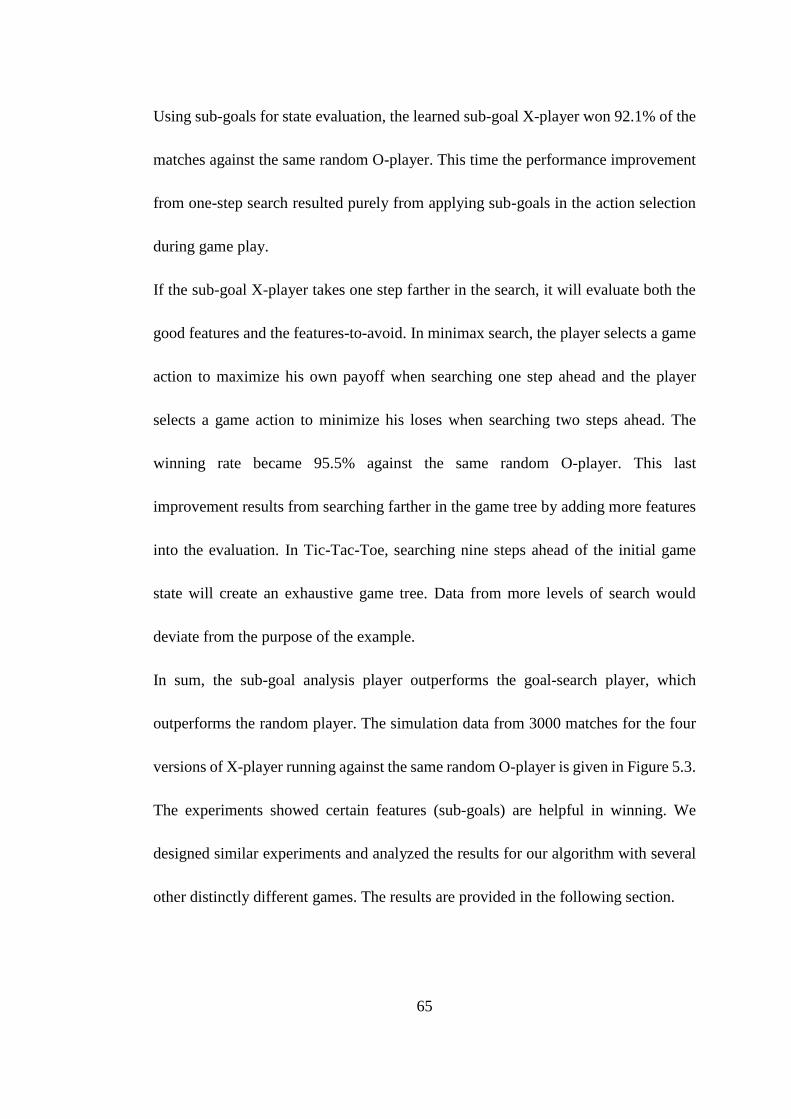
65

Using sub-goals for state evaluation, the learned sub-goal X-player won 92.1% of the

matches against the same random O-player. This time the performance improvement

from one-step search resulted purely from applying sub-goals in the action selection

during game play.

If the sub-goal X-player takes one step farther in the search, it will evaluate both the

good features and the features-to-avoid. In minimax search, the player selects a game

action to maximize his own payoff when searching one step ahead and the player

selects a game action to minimize his loses when searching two steps ahead. The

winning rate became 95.5% against the same random O-player. This last

improvement results from searching farther in the game tree by adding more features

into the evaluation. In Tic-Tac-Toe, searching nine steps ahead of the initial game

state will create an exhaustive game tree. Data from more levels of search would

deviate from the purpose of the example.

In sum, the sub-goal analysis player outperforms the goal-search player, which

outperforms the random player. The simulation data from 3000 matches for the four

versions of X-player running against the same random O-player is given in Figure 5.3.

The experiments showed certain features (sub-goals) are helpful in winning. We

designed similar experiments and analyzed the results for our algorithm with several

other distinctly different games. The results are provided in the following section.

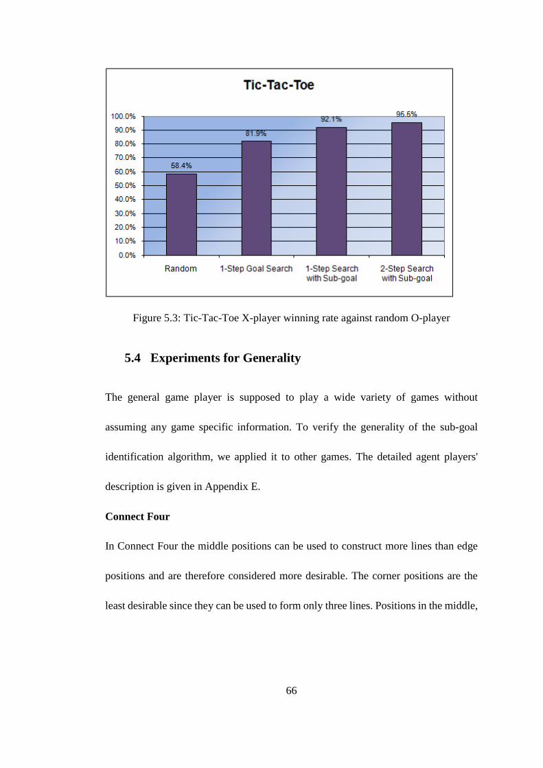
66

Figure 5.3: Tic-Tac-Toe X-player winning rate against random O-player

5.4 Experiments for Generality

The general game player is supposed to play a wide variety of games without

assuming any game specific information. To verify the generality of the sub-goal

identification algorithm, we applied it to other games. The detailed agent players'

description is given in Appendix E.

Connect Four

In Connect Four the middle positions can be used to construct more lines than edge

positions and are therefore considered more desirable. The corner positions are the

least desirable since they can be used to form only three lines. Positions in the middle,

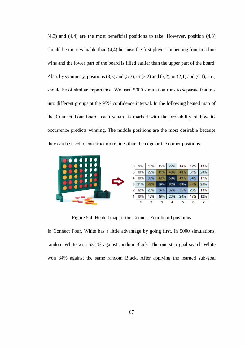
67

(4,3) and (4,4) are the most beneficial positions to take. However, position (4,3)

should be more valuable than (4,4) because the first player connecting four in a line

wins and the lower part of the board is filled earlier than the upper part of the board.

Also, by symmetry, positions (3,3) and (5,3), or (3,2) and (5,2), or (2,1) and (6,1), etc.,

should be of similar importance. We used 5000 simulation runs to separate features

into different groups at the 95% confidence interval. In the following heated map of

the Connect Four board, each square is marked with the probability of how its

occurrence predicts winning. The middle positions are the most desirable because

they can be used to construct more lines than the edge or the corner positions.

Figure 5.4: Heated map of the Connect Four board positions

In Connect Four, White has a little advantage by going first. In 5000 simulations,

random White won 53.1% against random Black. The one-step goal-search White

won 84% against the same random Black. After applying the learned sub-goal

68

information from the analysis, the learned White won 91% against the random Black

player. See the Connect Four results in Figure 5.6.

Mini-Chess

In Mini-Chess all pieces have the same movement rules as in regular Chess. It's

obvious to human players that if White King moves from its initial position (c,1) to

(b,2), the Black King can be pinned in the corner, creating a very promising situation

for checkmate. The agent was not aware of such strategy when the game started. But

after learning from its own history, it identifies the top three most desired sub-goals

from simulation. They are having White King take (b,2), and White Rook take (d,4)

and therefore pin Black King in (b,4).

Figure 5.5: Initial state of the Mini-Chess game and its top three sub-goals

In random playing, Black has higher chances to win the game since a random player

can hardly come up with a winning strategy. In 3000 matches, random White wins

30.5% against random Black (wins 69.5%). By searching goals one step ahead in the

simulations, White wins only 31.8%, due to the fact that a winning strategy takes

69

more than one step to develop. After applying the learned sub-goal information to

guide the search, the learned White wins 81% against the same random Black. See the

Mini-Chess results in Figure 5.6.

Farmer

In the Farmer game, each player can buy or sell one of the four commodities, grow or

make one of the four raw materials, or build one of the two infrastructures -- giving

the Farmer game a branching factor over 1000 on simultaneous moves (see Section

3.4). While the game tree search cannot possibly reach any goals more than a few

steps away, the sub-goal analysis correctly identifies important actions shared by the

winners. In 3000 random Farmer matches, we found the action building a factory

seriously negatively affects the cash flow and puts the player at a disadvantage in the

ten-iteration Farmer game. The player owns a factory in 21% of the matches he won.

But owning a factory is very beneficial in a 20-iteration Farmer game. The player

owns a factory in 95% of the matches he won. See the winning rate improvement for

the ten-iteration Farmer game in Figure 5.6.

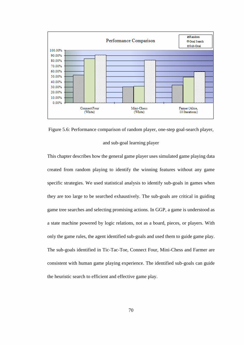
70

Figure 5.6: Performance comparison of random player, one-step goal-search player,

and sub-goal learning player

This chapter describes how the general game player uses simulated game playing data

created from random playing to identify the winning features without any game

specific strategies. We used statistical analysis to identify sub-goals in games when

they are too large to be searched exhaustively. The sub-goals are critical in guiding

game tree searches and selecting promising actions. In GGP, a game is understood as

a state machine powered by logic relations, not as a board, pieces, or players. With

only the game rules, the agent identified sub-goals and used them to guide game play.

The sub-goals identified in Tic-Tac-Toe, Connect Four, Mini-Chess and Farmer are

consistent with human game playing experience. The identified sub-goals can guide

the heuristic search to efficient and effective game play.

71

6 Decision Making in GGP

6.1 Grouping of Sub-Goals

A game may have hundreds or even thousands of features in its life cycle. The

existence of one individual feature provides some information about the game status

but often it is too isolated. Some features are more beneficial when combined with

certain other features. Some features are mutually exclusive and cannot co-exist.

Therefore, following influential features one after another may not lead the agent

towards the goals. In a game tree, every node is a game state and every game state is

composed of many features. A game state needs to be considered as one unit when

comparing to other states. This is the essential idea why the groupings of features are

needed.

Note that the purpose of the evaluation function is to guide the heuristic search. The

search needs to pick one action out of a list of available legal actions so that the

game can move forward. The evaluation function is looking for a preference order of

the states, not the exact value of the states. Payoff acts and is used as an ordinal

utility function. Agent behavior is preserved under any monotonic transformation of

72

the evaluation. We use a decision tree to get such a preference sequence of the game

states.

6.2 Decision Trees

A decision tree, also called classification tree or regression tree, is a widely used

machine learning algorithm. A decision tree takes a set of attributes as input and

outputs the predicted values for the input. It works as a predictive model to map the

target game states to numerical values according to existing observations. ID3

(Quinlan, 1986) and C4.5 (Quinlan, 1993) are well known decision tree algorithms.

The major improvements of C4.5 over ID3 are handling continuous attributes and

pruning trees after creation. We use C4.5 in this dissertation. The contents in this

section have been published (Sheng, 2011a, 2011b).

6.2.1 Decision Tree C4.5 Algorithm

The C4.5 algorithm calculates the information gain for each attribute in the training

set and selects the attribute with the highest gain value on which to split. The

splitting process partitions the training data into two groups, one with the splitting

attribute, one without it. New attributes are added iteratively into the decision tree as

tree nodes. The partition stops when majority voting can be established for the

outcome class. Figure 6.1 is the pseudo-code for creating the decision tree.

73

Figure 6.1: Pseudo-code for decision tree C4.5

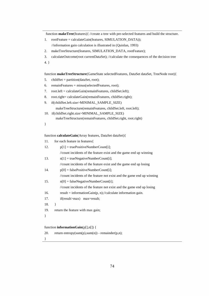
74

function makeTree(features){ //create a tree with pre-selected features and build the structure.

1. rootFeature = calculateGain(features, SIMULATION_DATA));

//information gain calculation is illustrated in (Quinlan, 1993)

2. makeTreeStructure(features, SIMULATION_DATA, rootFeature);

3. calculateOutcome(root currentDataSet); //calculate the consequences of the decision tree

4. }

function makeTreeStructure(GameState selectedFeatures, DataSet dataSet, TreeNode root){

5. childSet = partition(dataSet, root);

6. remainFeatures = minus(selectedFeatures, root);

7. root.left = calculateGain(remainFeatures, childSet.left);

8. root.right= calculateGain(remainFeatures, childSet.right);

9. if(childSet.left.size>MINIMAL_SAMPLE_SIZE)

makeTreeStructure(remainFeatures, childSet.left, root.left);

10. if(childSet.right.size>MINIMAL_SAMPLE_SIZE)

makeTreeStructure(remainFeatures, childSet.right, root.right)

}

function calculateGain(Array features, DataSet dataSet){

11. for each feature in features{

12. p[1] = truePositiveNumberCount[i];

//count incidents of the feature exist and the game end up winning

13. n[1] = trueNegativeNumberCount[i];

//count incidents of the feature exist and the game end up losing

14. p[0] = falsePositiveNumberCount[i];

//count incidents of the feature not exist and the game end up winning

15. n[0] = falseNegativeNumberCount[i];

//count incidents of the feature not exist and the game end up losing

16. result = informationGain(p, n);//calculate information gain.

17. if(result>max) max=result;

18. }

19. return the feature with max gain;

}

function informationGain(p[],n[]) {

20. return entropy(sum(p),sum(n)) - remainder(p,n);

}

75

function remainder(p[], n[]){//remainder = ∑(pi + ni)/(p+n) *entropy(pi,ni)

21. total = sum(p)+sum(n);

22. return sigma(((p[i]+n[i])/total)*entropy(p[i],n[i]));

}

function entropy(p, n) {

//entropy = ∑-P(vi)(log2P(vi), P is the probability of the result based on the feature value v

23. return prediction(p/(p+n), n/(p+n));

}

function prediction(p[]) {

24. return sigma(-p[i]*log2(p[i]));

}

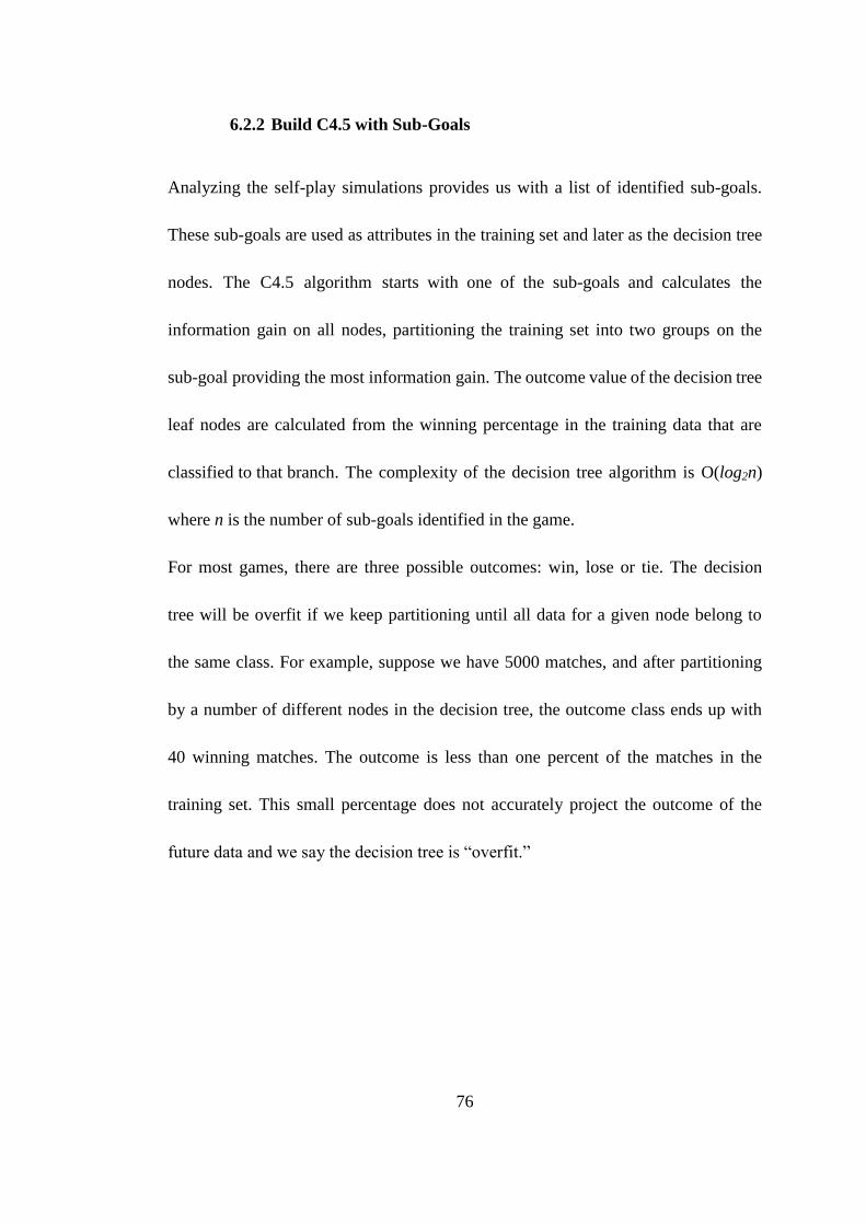
76

6.2.2 Build C4.5 with Sub-Goals

Analyzing the self-play simulations provides us with a list of identified sub-goals.

These sub-goals are used as attributes in the training set and later as the decision tree

nodes. The C4.5 algorithm starts with one of the sub-goals and calculates the

information gain on all nodes, partitioning the training set into two groups on the

sub-goal providing the most information gain. The outcome value of the decision tree

leaf nodes are calculated from the winning percentage in the training data that are

classified to that branch. The complexity of the decision tree algorithm is O(log2n)

where n is the number of sub-goals identified in the game.

For most games, there are three possible outcomes: win, lose or tie. The decision

tree will be overfit if we keep partitioning until all data for a given node belong to

the same class. For example, suppose we have 5000 matches, and after partitioning

by a number of different nodes in the decision tree, the outcome class ends up with

40 winning matches. The outcome is less than one percent of the matches in the

training set. This small percentage does not accurately project the outcome of the

future data and we say the decision tree is “overfit.”

77

To avoid overfitting, our agent calculates the outcome of the decision node from the

number of partitioned data for a given node. The node value is the percentage of the

simulation runs that the agent ends up winning. Figure 6.2 is a simplified decision

tree example for illustration purposes:

Figure 6.2: A decision-tree example

The decision tree example started with 5000 matches. According to the C4.5

calculation, feature A provides the most information gain at the beginning. There are

1527 matches out of the 5000 simulation runs that contain feature A and the rest do

not contain feature A. Then the algorithm decides that feature B provides the next

highest information gain and partition the data over feature B. There are 1352

78

matches contain feature B out of the 1527 matches that already contain feature A.

Among the 1352 matches that contain both feature A and feature B, 872 matches

turned out winning the game. Therefore, the left most bucket has a value of

875/1352 = 0.64. The rest of the nodes and buckets in the example are built with the

same method and have similar explanations.

The example demonstrates the creation of the decision tree and how the outcome

results are calculated. The creation process complexity is O(log2n) where n is the

number of game features. Once created, the tree is used for the entire game playing.

The actual decision tree in the GGP agent goes through additional processes such as

an overfitting test and pruning, but the overall cost of creating the decision tree is

considered linear in the game tree size.

6.2.3 Using Decision Tree for Evaluation

Using the decision tree for evaluating game states is straight forward. The agent

feeds game states covered by the search one at a time into the decision tree, to

determine into which outcome bucket they belong. The state value is the outcome

result of the tree. The pseudo-code of using the decision tree for state evaluation is

given in Figure 6.3.

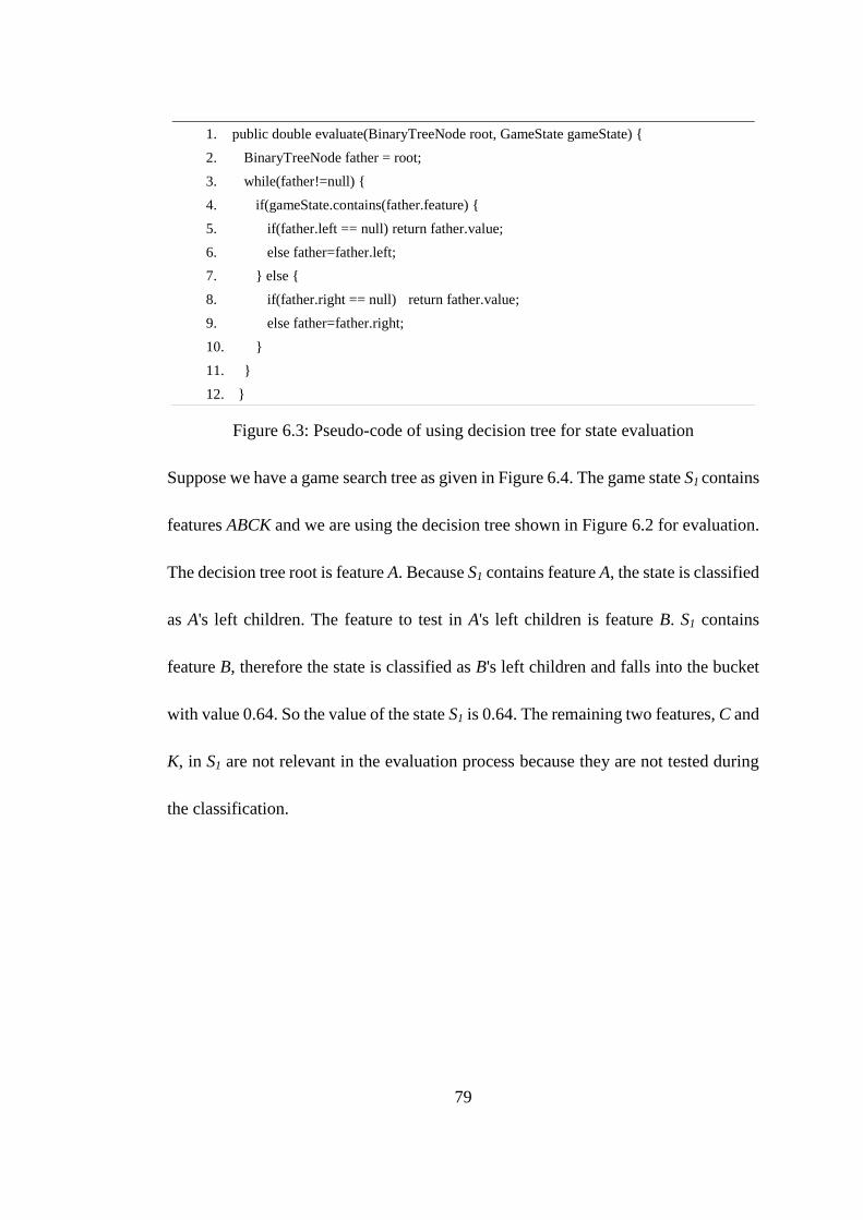
79

Figure 6.3: Pseudo-code of using decision tree for state evaluation

Suppose we have a game search tree as given in Figure 6.4. The game state S1 contains

features ABCK and we are using the decision tree shown in Figure 6.2 for evaluation.

The decision tree root is feature A. Because S1 contains feature A, the state is classified

as A's left children. The feature to test in A's left children is feature B. S1 contains

feature B, therefore the state is classified as B's left children and falls into the bucket

with value 0.64. So the value of the state S1 is 0.64. The remaining two features, C and

K, in S1 are not relevant in the evaluation process because they are not tested during

the classification.

1. public double evaluate(BinaryTreeNode root, GameState gameState) {

2. BinaryTreeNode father = root;

3. while(father!=null) {

4. if(gameState.contains(father.feature) {

5. if(father.left == null) return father.value;

6. else father=father.left;

7. } else {

8. if(father.right == null) return father.value;

9. else father=father.right;

10. }

11. }

12. }

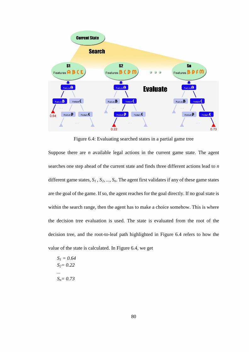
80

Figure 6.4: Evaluating searched states in a partial game tree

Suppose there are n available legal actions in the current game state. The agent

searches one step ahead of the current state and finds three different actions lead to n

different game states, S1 , S2, ..., Sn. The agent first validates if any of these game states

are the goal of the game. If so, the agent reaches for the goal directly. If no goal state is

within the search range, then the agent has to make a choice somehow. This is where

the decision tree evaluation is used. The state is evaluated from the root of the

decision tree, and the root-to-leaf path highlighted in Figure 6.4 refers to how the

value of the state is calculated. In Figure 6.4, we get

S1 = 0.64

S2= 0.22

…

Sn= 0.73

81

Thus the action n is the most promising choice to win the game.

The outcome of the decision tree evaluation is used to guide the minimax search in our

GGP agent. Suppose in a given time frame, the minimax search explored 500 nodes in

a game tree. There are 370 nodes that have both ancestors and successors, and the

remaining 130 have only ancestors but not successors. These 130 nodes are called leaf

nodes in the search tree. The decision tree evaluation is only applicable to these leaf

nodes. The value of the intermediate nodes will be calculated using backward

chaining in the minimax search. From the example scenario, we can conclude that the

time consumption of using the decision tree for evaluation is m*O(n), where m is the

total steps to finish a game and n is the game tree nodes searched in every step.

6.2.4 Decision Tree Learning versus Individual Sub-Goal Learning

For our study, we set up four different agents to play against the same random dummy

opponent, so that the agent's performance can be evaluated against the same criteria.

The agents take the role of the first player to move (Farmer has simultaneous moves)

in the following examples. If we had set up other players to be the second player in the

game with decision tree learning, the performance improvements would be just as

convincing. The detailed agent players' description is given in Appendix E. The four

agents are:

82

The random player;

The goal-search player that searches for goal states one step ahead of the

current state;

The sub-goal learning player that searches one step ahead and uses sub-goal

learning for state values;

The decision tree player that searches one step ahead and use the decision tree

for state evaluation.

Mini-Chess (Figure 3.4A)

Mini-Chess could have been exhaustively searched, but we deliberately avoid that for

example purposes. In Mini-Chess, the random White player or the one step

goal-search player has only a small chance to win over random Black because it is

hard to form an attacking strategy without planning. The third agent uses sub-goals as

the evaluation criteria to guide the search. When the actual goals defined in the game

description are not within the search range, the agent considers putting certain Chess

pieces on certain positions as sub-goals (e.g. putting white king at position (b, 2) is

one high value sub-goal), and taking actions toward these sub-goals. The performance

improvement for the sub-goal learning player is due to adding the sub-goal learning

layer to the one-step goal-search.

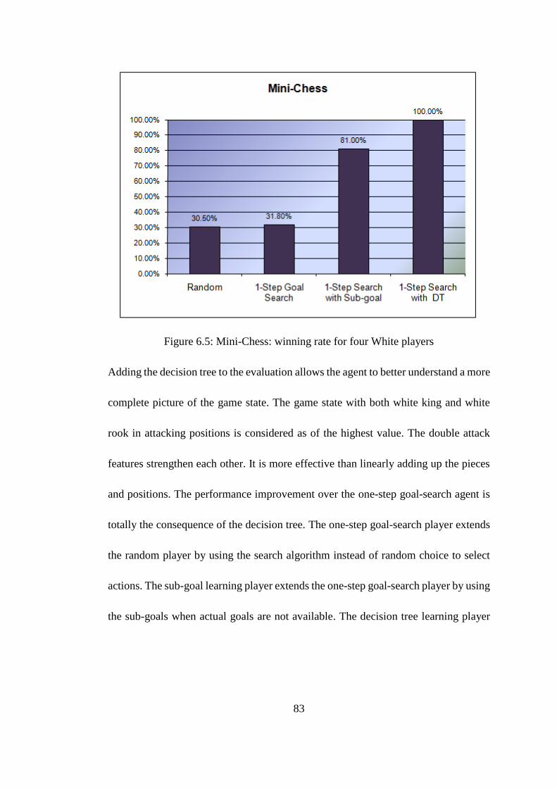
83

Figure 6.5: Mini-Chess: winning rate for four White players

Adding the decision tree to the evaluation allows the agent to better understand a more

complete picture of the game state. The game state with both white king and white

rook in attacking positions is considered as of the highest value. The double attack

features strengthen each other. It is more effective than linearly adding up the pieces

and positions. The performance improvement over the one-step goal-search agent is

totally the consequence of the decision tree. The one-step goal-search player extends

the random player by using the search algorithm instead of random choice to select

actions. The sub-goal learning player extends the one-step goal-search player by using

the sub-goals when actual goals are not available. The decision tree learning player

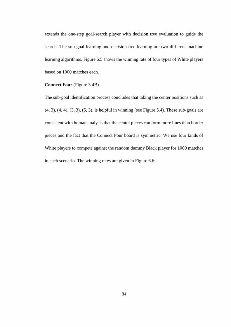
84

extends the one-step goal-search player with decision tree evaluation to guide the

search. The sub-goal learning and decision tree learning are two different machine

learning algorithms. Figure 6.5 shows the winning rate of four types of White players

based on 1000 matches each.

Connect Four (Figure 3.4B)

The sub-goal identification process concludes that taking the center positions such as

(4, 3), (4, 4), (3, 3), (5, 3), is helpful in winning (see Figure 5.4). These sub-goals are

consistent with human analysis that the center pieces can form more lines than border

pieces and the fact that the Connect Four board is symmetric. We use four kinds of

White players to compete against the random dummy Black player for 1000 matches

in each scenario. The winning rates are given in Figure 6.6:

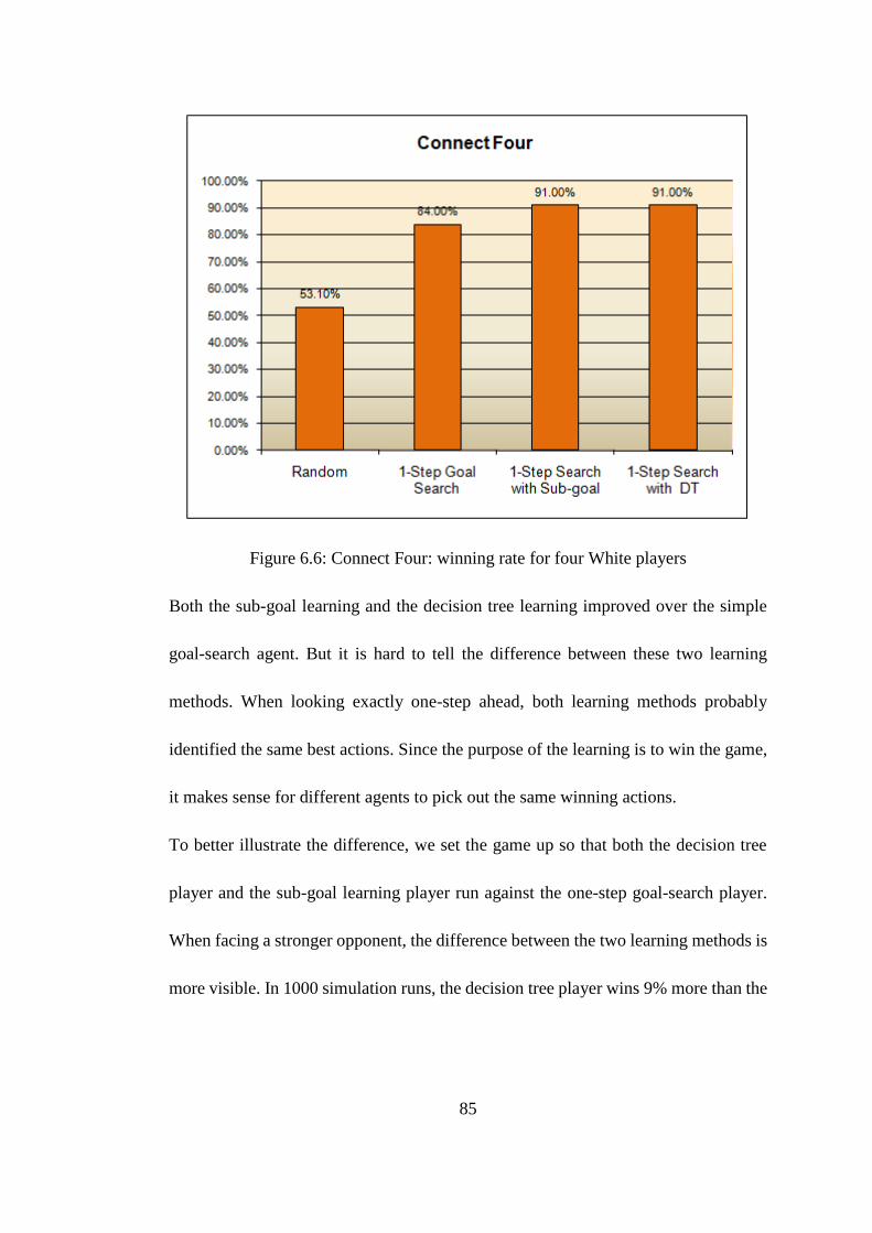
85

Figure 6.6: Connect Four: winning rate for four White players

Both the sub-goal learning and the decision tree learning improved over the simple

goal-search agent. But it is hard to tell the difference between these two learning

methods. When looking exactly one-step ahead, both learning methods probably

identified the same best actions. Since the purpose of the learning is to win the game,

it makes sense for different agents to pick out the same winning actions.

To better illustrate the difference, we set the game up so that both the decision tree

player and the sub-goal learning player run against the one-step goal-search player.

When facing a stronger opponent, the difference between the two learning methods is

more visible. In 1000 simulation runs, the decision tree player wins 9% more than the

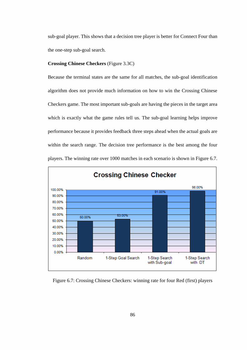
86

sub-goal player. This shows that a decision tree player is better for Connect Four than

the one-step sub-goal search.

Crossing Chinese Checkers (Figure 3.3C)

Because the terminal states are the same for all matches, the sub-goal identification

algorithm does not provide much information on how to win the Crossing Chinese

Checkers game. The most important sub-goals are having the pieces in the target area

which is exactly what the game rules tell us. The sub-goal learning helps improve

performance because it provides feedback three steps ahead when the actual goals are

within the search range. The decision tree performance is the best among the four

players. The winning rate over 1000 matches in each scenario is shown in Figure 6.7.

Figure 6.7: Crossing Chinese Checkers: winning rate for four Red (first) players

87

Farmer (Figure 3.4D)

The Farmer game is very flexible. The game can be easily reconfigured from three

players to two, four or more players. It can be changed from 10 iterations to 20, 40 or

more iterations. The game dynamics change accordingly. For example, in a

ten-iteration game, building a factory is not a good choice because the player has

spent a significant portion of his money for the factory which does not leave much to

buy raw materials and there is not adequate time to recoup the expense. But in the 40

iteration game, the cost of building a factory is almost nothing compared to the

skyrocketing price of the commodities the player can sell in the later part of the game.

For the three-player ten-iteration Farmer game, the sub-goal identification recognized

some basic winning factors including having a farm, not having a factory, and not

keeping any inventory when the game ends. By setting up the same four agents for

player Alice, and using random dummy players for Barney and Charlie, we get the

simulation winning rate over 1000 matches in each scenario in Figure 6.8.

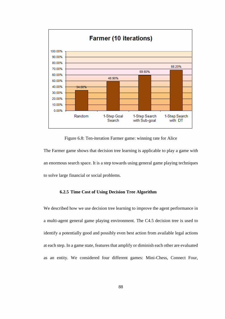
88

Figure 6.8: Ten-iteration Farmer game: winning rate for Alice

The Farmer game shows that decision tree learning is applicable to play a game with

an enormous search space. It is a step towards using general game playing techniques

to solve large financial or social problems.

6.2.5 Time Cost of Using Decision Tree Algorithm

We described how we use decision tree learning to improve the agent performance in

a multi-agent general game playing environment. The C4.5 decision tree is used to

identify a potentially good and possibly even best action from available legal actions

at each step. In a game state, features that amplify or diminish each other are evaluated

as an entity. We considered four different games: Mini-Chess, Connect Four,

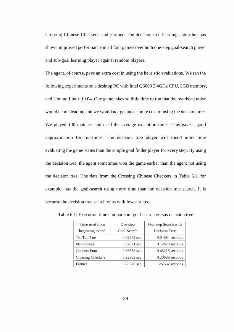
89

Crossing Chinese Checkers, and Farmer. The decision tree learning algorithm has

shown improved performance in all four games over both one-step goal-search player

and sub-goal learning player against random players.

The agent, of course, pays an extra cost in using the heuristic evaluations. We ran the

following experiments on a desktop PC with Intel Q6600 2.4GHz CPU, 2GB memory,

and Ubuntu Linux 10.04. One game takes so little time to run that the overhead noise

would be misleading and we would not get an accurate cost of using the decision tree.

We played 100 matches and used the average execution times. This gave a good

approximation for run-times. The decision tree player will spend more time

evaluating the game states than the simple goal finder player for every step. By using

the decision tree, the agent sometimes won the game earlier than the agent not using

the decision tree. The data from the Crossing Chinese Checkers in Table 6.1, for

example, has the goal-search using more time than the decision tree search. It is

because the decision tree search wins with fewer steps.

Table 6.1: Execution time comparison: goal-search versus decision tree

Time used from

beginning to end

One-step

Goal-Search

One-step Search with

Decision Tree

Tic-Tac-Toe 0.02872 sec. 0.04694 seconds

Mini-Chess 0.07871 sec. 0.12423 seconds

Connect Four 0.36538 sec. 0.45216 seconds

Crossing Checkers 0.22302 sec. 0.20699 seconds

Farmer 22.220 sec. 26.632 seconds

90

6.2.6 Overfitting Concerns

The decision tree learning algorithm considers features in one game state as a unit and

evaluates the state weight as an entirety. Experiments showed the decision tree

algorithm improved the winning rate significantly for small games such as

Mini-Chess, Tic-Tac-Toe, and Crossing Chinese Checkers. However, the

improvement generated by the decision tree learning for larger size games is not as

clear. Our experiments were based on very limited game tree search. This allowed us

to isolate the improvement attributable to learning algorithms from the effect of

deeper searches. Searching more game tree nodes in the game playing certainly

enables the machine learning algorithms to make more informed decision.

Another challenge is that the decision tree is based on the entire game. In large games,

the differences of the states reached by different moves in one step can be quite trivial

compared to the whole game process. These trivial differences lead to the situation

that several game states are classified into the same outcome bucket of a decision tree

and therefore make it impossible to differentiate a good action from one that is not so

good. Of course, we can always let the decision tree grow and split on more nodes.

There always exist enough features on which to split. But it would eventually come to

a threshold where unimportant features would be magnified so as to reach misleading

conclusions. This small percentage of results used in the decision relative to the total

91

size of the decision space would not accurately predict the outcome. Overfitted

decision trees do not provide good guidance for the learning algorithm, but it is not

clear how to avoid overfitting. This is the motivation for investigating and improving

the decision tree learning algorithm so that we can effectively solve larger problems.

6.3 Contextual Decision Tree

6.3.1 Decisions Bounded by Search

Overfitting is not a simple question and there are numerous publications about

avoiding overfitting in decision trees (Schaffer, 1993; Mingers 1989; Bramer, 2007).

However, from the game playing perspective, the decision tree pruning would

eliminate the trivial differences in the data. We cannot get the preference order of the

game states. Machine learning is necessary in game playing only when the game is

too large to be searched exhaustively. Why bother guessing with learning if searching

the game tree provides definitive decisions to good actions? Decision making in

game playing is always integrated with the game tree search. The search algorithm

reveals information about the future of the game and the learning algorithm evaluates

the searched game states and provides feedback to the search. There exists no

decision making for the entire game but only in the context of the current search

92

range. The decision making is bound within the searched range that changes from

step-to-step.

Introducing contextual, or dynamic, decision trees enables the decision making

process to function effectively within the context of the search range. It is an

extension of the decision tree learning in the last section. When the game tree is only

partially revealed by the search, there may exist no utility that is important in the

entire game. By addressing the local utility in the context of the current game state

and the current search range, the agent is able to reach pragmatic decisions in every

step while limited by search time and space. Based on the available partial picture,

the agent is capable of making appropriate and timely decisions given the context.

A general game playing agent, by definition, is supposed to play a wide variety of

different games. In order to do this, the machine learning algorithms must scale well

as the game size grows. We propose decision making based on the context of the

decision in order to address large complicated games. The contents in this section

have been published (Sheng, 2011d).

6.3.2 Building Contextual Decision Trees

The agent's purpose for searching a game tree and evaluating the game states

encountered during the search is to select an action that has the best potential of

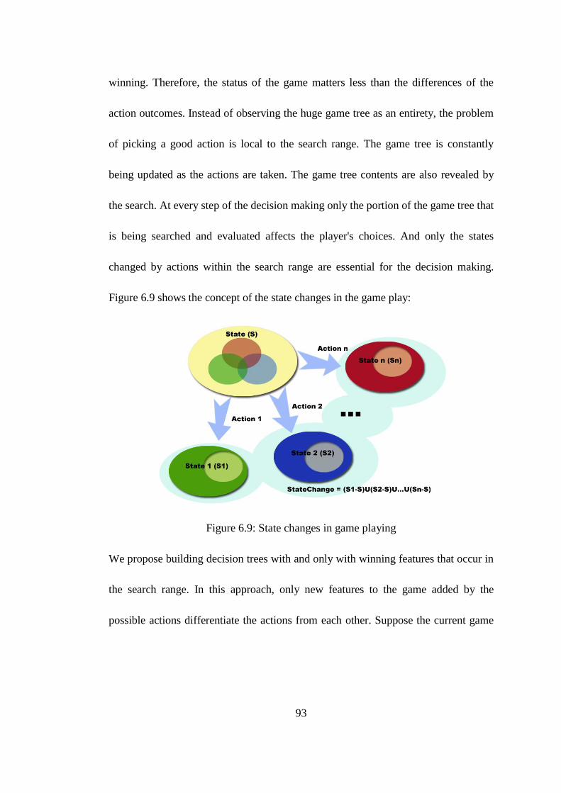
93

winning. Therefore, the status of the game matters less than the differences of the

action outcomes. Instead of observing the huge game tree as an entirety, the problem

of picking a good action is local to the search range. The game tree is constantly

being updated as the actions are taken. The game tree contents are also revealed by

the search. At every step of the decision making only the portion of the game tree that

is being searched and evaluated affects the player's choices. And only the states

changed by actions within the search range are essential for the decision making.

Figure 6.9 shows the concept of the state changes in the game play:

Figure 6.9: State changes in game playing

We propose building decision trees with and only with winning features that occur in

the search range. In this approach, only new features to the game added by the

possible actions differentiate the actions from each other. Suppose the current game

94

state S contains a group of features. The available legal actions a1, a2, ... an lead to the

states S1, S2, ... Sn. Each of outcome states, Si, inherited some subset of features from

S but also contain some new features of its own. These states need to be evaluated by

the learning algorithm for their winning potentials. The feature set StateChange,

contains the differences added by these actions, can be given as:

StateChange = (S1-S) ∪ (S2-S) ∪ ... ∪ (Sn-S)

The differences of the action outcomes are amplified from making a small impact

over the entire game to making a strong impact over the action selection. The state

values calculated from the decision tree will not be consistent from step to step.

Instead, the state values become relative and are only meaningful to the states against

which it is being compared. The pseudo-code of implementing the contextual

decision tree is given in Figure 6.10.

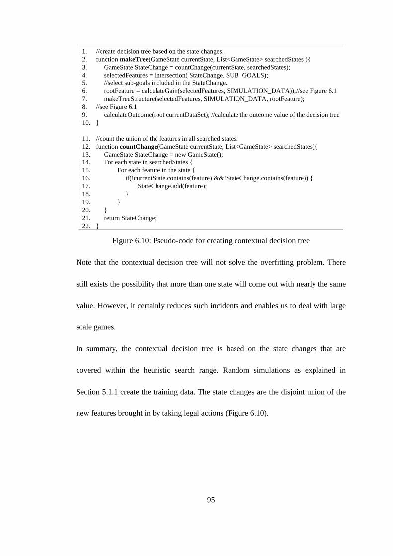
95

1. //create decision tree based on the state changes.

2. function makeTree(GameState currentState, List<GameState> searchedStates ){

3. GameState StateChange = countChange(currentState, searchedStates);

4. selectedFeatures = intersection( StateChange, SUB_GOALS);

5. //select sub-goals included in the StateChange.

6. rootFeature = calculateGain(selectedFeatures, SIMULATION_DATA));//see Figure 6.1

7. makeTreeStructure(selectedFeatures, SIMULATION_DATA, rootFeature);

8. //see Figure 6.1

9. calculateOutcome(root currentDataSet); //calculate the outcome value of the decision tree

10. }

11. //count the union of the features in all searched states.

12. function countChange(GameState currentState, List<GameState> searchedStates){

13. GameState StateChange = new GameState();

14. For each state in searchedStates {

15. For each feature in the state {

16. if(!currentState.contains(feature) &&!StateChange.contains(feature)) {

17. StateChange.add(feature);

18. }

19. }

20. }

21. return StateChange;

22. }

Figure 6.10: Pseudo-code for creating contextual decision tree

Note that the contextual decision tree will not solve the overfitting problem. There

still exists the possibility that more than one state will come out with nearly the same

value. However, it certainly reduces such incidents and enables us to deal with large

scale games.

In summary, the contextual decision tree is based on the state changes that are

covered within the heuristic search range. Random simulations as explained in

Section 5.1.1 create the training data. The state changes are the disjoint union of the

new features brought in by taking legal actions (Figure 6.10).

96

6.3.3 Using Contextual Decision Trees for State Evaluation

To evaluate the effectiveness of the contextual decision trees, we compare it against

our previous agents to isolate the benefits introduced by the contextual decision trees.

We also compared it against other widely available agents published at the GGP

website and against other benchmark scenarios. Finally, the costs and the benefits are

discussed.

6.3.3.1 Comparison with Other Learning Algorithms

The agent using the contextual decision tree is compared among five agents that

take random actions;

search one step ahead for goals;

search one step ahead for goals; if goals are not in the search range, use

sub-goal learning to evaluate the states;

search one step ahead for goals; if goals are not in the search range, use

decision tree learning to evaluate the states;

search one step ahead for goals; if goals are not in the search range, use

contextual decision tree learning to evaluate the states;

A detailed agent players' description is given in Appendix E. We use Tic-Tac-Toe,

Connect Four (with the branching factor 7 and possible positions 342

), Othello (with

97

the branching factor of 8-12 and possible positions 364

), and the three-player

non-zero-sum simultaneous eCommerce game Farmer (branching factor ~1000) as

benchmarks. The agent is set up to be the first player in all four games. If we had set

up the contextual decision tree learning as the second player in the game, the

performance improvements would be just as convincing.

In the first column of every game in Figure 6.11, the player makes random decisions.

In the second column, the player searches one step ahead of the current game state for

the goals and makes random decisions when the goals are not found. The performance

improvement is due to the goal-search. In the third column, the player uses sub-goal

values in the one-step search. The improvement is attributable to using sub-goals to

guide the search when the actual goals are not within the search range. This shows that

the sub-goals are correctly identified and are helpful in winning. In the fourth column,

the player uses decision tree learning that shows groupings of the features are more

useful to winning than individual features. In the fifth column of each game, the agent

uses contextual decision trees. The performance improvement, especially in

large-size games, is attributable to considering the action results within the search

context.

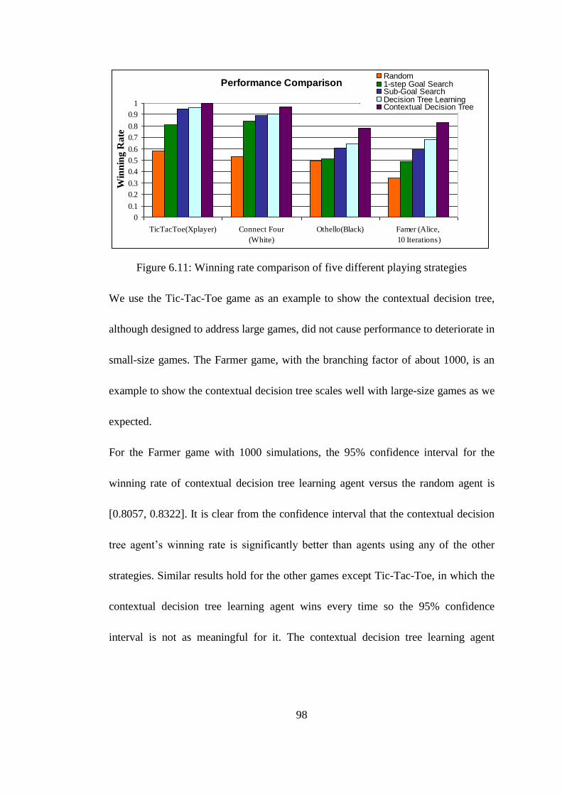
98

Performance Comparison

0

0.1

0.2

0.3

0.4

0.5

0.6

0.7

0.8

0.9

1

TicTacToe(Xplayer) Connect Four

(White)

Othello(Black) Famer (Alice,

10 Iterations)

Win

nin

g R

ate

Random1-step Goal SearchSub-Goal SearchDecision Tree LearningContextual Decision Tree

Figure 6.11: Winning rate comparison of five different playing strategies

We use the Tic-Tac-Toe game as an example to show the contextual decision tree,

although designed to address large games, did not cause performance to deteriorate in

small-size games. The Farmer game, with the branching factor of about 1000, is an

example to show the contextual decision tree scales well with large-size games as we

expected.

For the Farmer game with 1000 simulations, the 95% confidence interval for the

winning rate of contextual decision tree learning agent versus the random agent is

[0.8057, 0.8322]. It is clear from the confidence interval that the contextual decision

tree agent’s winning rate is significantly better than agents using any of the other

strategies. Similar results hold for the other games except Tic-Tac-Toe, in which the

contextual decision tree learning agent wins every time so the 95% confidence

interval is not as meaningful for it. The contextual decision tree learning agent

99

showed significant improvement over the other strategies in each of the three

large-size games.

Limited experiments also showed that when the agent searches deeper, the learning

algorithm benefits more. When Othello plays against the goal-search player with both

players searching one level ahead, the dynamic decision tree wins 53% percent, a

little better than the goal-search player. But when both player search three levels

ahead with minimax, the dynamic decision tree player defeats the goal-search player

64% of the time. With more nodes covered in the search range, more new features are

introduced and more states are evaluated. The contextual decision making is more

beneficial when provided with more information.

6.3.3.2 Comparison with Other Widely Available GGP Players

The GGP website maintained by Dresden University of Technology provides an

excellent platform to test agents on a wide variety of games and play against other

intelligent agents. In playing against other GGP players, our results can be described

in the following three categories:

For single-player games, three-person prisoner's dilemma game variation, and

Mini-Chess, our player achieved nearly a 100% winning rate. Because our

100

agent is based on feature analysis, once a feasible solution is found, the agent

would follow the winning path in the next match.

For Tic-Tac-Toe like games (small-size two-player games), our agent always

ties with the competing agent. The reason is that if both players play well, tie

is the optimal solution for each of them, no matter who goes first. In the past

experiments, we have not encountered even one match that did not tie

Tic-Tac-Toe when playing against an intelligent agent. We consider this result

as the optimal outcome of the game.

For more complicated games such as Connect Four or Othello, our player wins

more when the playing interval between the steps is set shorter and wins less

with longer playing intervals. In the game process, the playing interval is used

for heuristic search. When both players search only a few nodes in short

playing intervals, our agent has a better learning algorithm to differentiate the

good actions from the not-so-good ones. In the GGP area, Monte Carlo Tree

Search is considered by far to be the most effective searching algorithm

(Finnsson, 2011; Gudmundsson, 2011; Méhat, 2010; Kroeker, 2011). We are

aware that our search algorithm (minimax) is not optimal and obviously needs

improvement but the focus of our research has been on the learning algorithms

as opposed to the search.

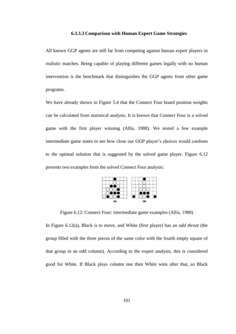
101

6.3.3.3 Comparison with Human Expert Game Strategies

All known GGP agents are still far from competing against human expert players in

realistic matches. Being capable of playing different games legally with no human

intervention is the benchmark that distinguishes the GGP agents from other game

programs.

We have already shown in Figure 5.4 that the Connect Four board position weights

can be calculated from statistical analysis. It is known that Connect Four is a solved

game with the first player winning (Allis, 1988). We tested a few example

intermediate game states to see how close our GGP player’s choices would conform

to the optimal solution that is suggested by the solved game player. Figure 6.12

presents two examples from the solved Connect Four analysis:

Figure 6.12: Connect Four: intermediate game examples (Allis, 1988)

In Figure 6.12(a), Black is to move, and White (first player) has an odd threat (the

group filled with the three pieces of the same color with the fourth empty square of

that group in an odd column). According to the expert analysis, this is considered

good for White. If Black plays column one then White wins after that, so Black

102

should avoid column one. In Figure 6.12(b), it is White’s move. There are four

columns with an odd number of empty squares (slots). According to the solved

Connect Four player, White is supposed to move in one of these four columns (1, 3,

5, 7).

The GGP agent does not have the human knowledge of the odd threat or even square

numbers. But with the feedback from search and learning, our GGP agent correctly

identifies taking column one in 6.12(a) and taking column two or six in 6.12(b) has

adverse effects and avoids them. The GGP agent also identifies the first player's first

step should be to take column four, which has been considered by the solved player

as an optimal choice for the first step. These scenario examples show that, although

far from competing against human experts, our GGP agent makes reasonably good

actions in Connect Four, a game with a large number, 342

(~1020

), of possible

positions.

6.3.4 Time Cost of Contextual Decision Trees

The GGP agents need to allocate the limited resources to different tasks including

logic reasoning, game tree search, game state evaluation, and learning. The agent

pays extra cost to use an advanced learning algorithm and a good learning algorithm

should bring noticeable results with less noticeable costs. Because the time spent on

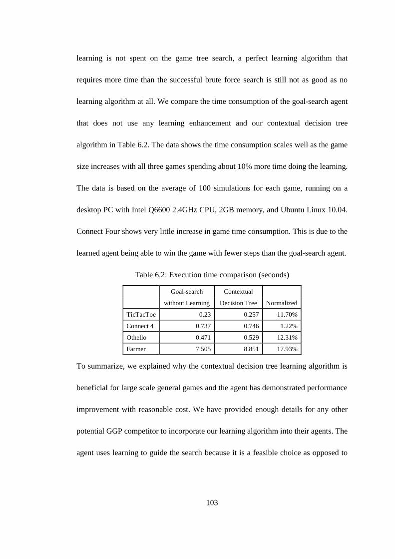
103

learning is not spent on the game tree search, a perfect learning algorithm that

requires more time than the successful brute force search is still not as good as no

learning algorithm at all. We compare the time consumption of the goal-search agent

that does not use any learning enhancement and our contextual decision tree

algorithm in Table 6.2. The data shows the time consumption scales well as the game

size increases with all three games spending about 10% more time doing the learning.

The data is based on the average of 100 simulations for each game, running on a

desktop PC with Intel Q6600 2.4GHz CPU, 2GB memory, and Ubuntu Linux 10.04.

Connect Four shows very little increase in game time consumption. This is due to the

learned agent being able to win the game with fewer steps than the goal-search agent.

Table 6.2: Execution time comparison (seconds)

Goal-search Contextual

Normalized without Learning Decision Tree

TicTacToe 0.23 0.257 11.70%

Connect 4 0.737 0.746 1.22%

Othello 0.471 0.529 12.31%

Farmer 7.505 8.851 17.93%

To summarize, we explained why the contextual decision tree learning algorithm is

beneficial for large scale general games and the agent has demonstrated performance

improvement with reasonable cost. We have provided enough details for any other

potential GGP competitor to incorporate our learning algorithm into their agents. The

agent uses learning to guide the search because it is a feasible choice as opposed to

104

searching the complete game tree. Our learning algorithm heuristics sacrifices the

accuracy of complete game tree search in exchange for efficiency.

105

7 Beyond the Current GGP Framework

GDL language enables various game definitions in the GGP framework. However,

GDL was designed with inherent limitations. The limitation to "finite, discrete,

deterministic multi-player games of complete information" (Love, 2005) was

proposed to simplify the problem set to facilitate research. But as the GGP research

developed in the past few years, the research advances have out grown the limited

definition. There have been attempts to extend GDL to include non-deterministic,

incomplete information games (Thielscher, 2010). We have proposed the extension to

include coalition games. The contents in this chapter have been published (Sheng,

2011c; Sheng, 2011e).

7.1 Issues with the Current GDL

Game playing is limited by time and space resources. Most games are not

exhaustively searchable. The agents need to allocate the limited time to logic

reasoning, game tree search, the action payoff evaluation, machine learning, and

game states transition, etc. Logic reasoning participates in all these operations. Small

performance improvements in the reasoning process can be greatly amplified to

106

expedite searches and learning and can therefore generate huge advancements in the

agent's performance (see Chapter 4)

In addition to the logic resolution data structure, we discovered how a game is written

affects the reasoning performance as well. For example, to determine if there exists a

line in Tic-Tac-Toe, the function can be written either as "find out all lines on the

board, and check if one is owned by myself", or as "find out all my pieces, and check

if any three formed a line.” The computational complexity is different in these two

expressions. In big games, some expressions can become so computationally

demanding that the wanted function cannot be reasonably defined.

7.1.1 Burden of the Natural Numbers

The Farmer game is a three-player simultaneous non-zero-sum financial game in

which each player tries to maximize his own net worth. In a financial game with items

to buy and sell, arithmetic addition and subtraction are used to calculate the gold

amount. Natural numbers are not naturally as part of GDL. Instead, the arithmetic

operations are defined as part of the game rules. Figure 7.1 is part of the Farmer game

that defines the addition operations of natural numbers. Bold indicates the first

definition of a function.

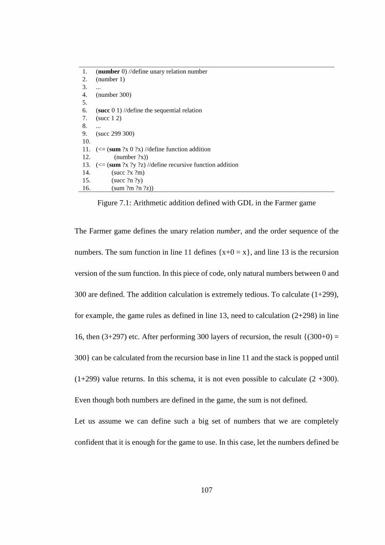
107

1. (number 0) //define unary relation number

2. (number 1)

3. ...

4. (number 300)

5.

6. (succ 0 1) //define the sequential relation

7. (succ 1 2)

8. ...

9. (succ 299 300)

10.

11. (<= (sum ?x 0 ?x) //define function addition

12. (number ?x))

13. (<= (sum ?x ?y ?z) //define recursive function addition

14. (succ ?x ?m)

15. (succ ?n ?y)

16. (sum ?m ?n ?z))

Figure 7.1: Arithmetic addition defined with GDL in the Farmer game

The Farmer game defines the unary relation number, and the order sequence of the

numbers. The sum function in line 11 defines {x+0 = x}, and line 13 is the recursion

version of the sum function. In this piece of code, only natural numbers between 0 and

300 are defined. The addition calculation is extremely tedious. To calculate (1+299),

for example, the game rules as defined in line 13, need to calculation (2+298) in line

16, then (3+297) etc. After performing 300 layers of recursion, the result {(300+0) =

300} can be calculated from the recursion base in line 11 and the stack is popped until

(1+299) value returns. In this schema, it is not even possible to calculate (2 +300).

Even though both numbers are defined in the game, the sum is not defined.

Let us assume we can define such a big set of numbers that we are completely

confident that it is enough for the game to use. In this case, let the numbers defined be

108

n, the time complexity for the number or succ function are O(n), so the recursion

addition calculation as defined in line 13 has the time complexity of O(n2). A simple

arithmetic addition operation is expected to be conducted in O(1) time. The current

GDL structure is obviously not satisfactory in terms of computational requirements.

7.1.2 Confusion of the Comparison

Although natural numbers are not defined as a GDL component, they are loosely used

in the goal definition in many games. For example, in Tic-Tac-Toe, when a player

forms a line, it is rewarded with 100 points with the rule (<= (goal ?player 100)

(line ?player)), and is rewarded with 0 points when the opponent forms a line. In both

situations, the numbers were used without being defined. To pursue the desired goals,

the agent needs to determine which goal is more desirable. For the current practice,

agents are assuming 100 is better than 0 without any logic definitions to support it.

In logic operations, which term is used does not affect the logic relations as long as the

changes are consistent. Anything that is not defined as a keyword in GDL is

substitutable. In fact, in the GGP competitions, to avoid human cheating, all the

competition games were scrambled into random, meaningless letter combinations.

The agent, operating correctly, can perform the same logic inference on the scrambled

109

version. As long as the logic relations are the same, the scrambled version of the game

will be treated the same.

Since substitution is not supposed to change the logic relations, GDL code (<=

(goal ?player 100) (line ?player)) can be substituted to (<= (goal ?player sss)

(line ?player)) as long as all the definitions and usages of the constant 100 are

substituted with sss universally. In many games, 100 (or 0) is used without definition.

Although the numerical goal rewards have never been scrambled in the past

competitions since they are used as regular logic symbols, they are not defined as

keywords and are subjected to the scramble operation just like any other symbol. Now

the agent is facing a logic resolution loophole: is the goal sss more desirable than the

goal ttt?

In some situations where the players are given partial credit, such as moving four

pieces into the designated place and getting 25 points for each piece, it is not possible

to choose one goal over another without knowing the values of the goals.

To define the goals more rigorously, the game needs to define unary relation number

as in Figure 7.1. It also needs to define a greater function for the agent to compare the

value of 100 and 0. The agent can order all the goal definitions and determine which

one is most desirable. Only in this way, can the agent calculate the partial credit for

completing partial tasks.

110

7.1.3 Challenge of Infinity

The finite set of natural numbers is hard enough for GDL to handle. When the content

of the game element involves an infinite set, the existing structure faces new

challenges. In the Farmer game, the market price of each commodity automatically

increases with the inflation factor at the end of every iteration as time goes by.

Suppose the inflation factor is 10% of the current price. Then the wheat price with no

transaction influence is 4 gold pieces in the first step, 4.4 in the second, 4.84 in the

third, 5.324 in fourth, and so on.

In GDL, it is still possible to define the natural numbers or a subset of real numbers by

defining the computational elements, such as the carry flag, the borrow flag, the

negative sign, etc. But for the real number infinity set, there does not exist a

reasonable way to describe such a scenario.

We can go on with the limitations of GDL and how to better use it to define an infinite

set by proposing a overflow threshold just like all computer systems do. But the

discussion of how to define more powerful scenarios within GDL misses the point.

GDL structure is for accommodating heterogeneous games in one multi-agent system

for the player agents to play. Re-writing of these computer games with GDL is not

only cumbersome but also not necessary.

111

7.2 Extension Implementation

GDL describes the basic game elements such as game initialization (keyword init),

state transition (keyword next), legal actions (keyword legal), game roles (keyword

role), game goals (keyword goal), game termination (keyword terminal), etc.

Researchers have written about 40 games with more than 200 variations with GDL.

GDL was never meant to be a closed system. There have been efforts to extend GDL

to describe new groups of games. New keywords sees and random were introduced in

order to add incomplete information games (Thielscher, 2010). New keywords

message, receive, send, time were added to describe market trading scenarios

(Thielscher, 2009b). Adding new keywords and a new group of games to the GGP

family certainly enriches this area. However, the process can be generalized in a

manner that makes new game definitions much easier, simpler, and clearer.

We propose adding the keywords include and use into GDL. Just like importing

packages in the Java language, or including the header files in C++, the include

keyword in GDL serves as an interface allowing area specific definitions and

functions to be shared and quoted without affecting the generality of GDL. The

include keyword serves as the information facade that bridges the game logic

representations described with GDL and the area specific contents. The keyword use

is to call external functions with parameters.

112

The major contribution of the extension is that an existing game does not have to be

completely re-written into GDL for the general game player to play. A game does not

have to be written in one computer language either. Certain game information (see

Section 7.5) can be defined and calculated in the user's favorite programming

languages and passed back and forth through a command line interface.

We now use the piece of code in Figure 7.1 of the Farmer game again as an example

for how arithmetic can be introduced with the include interface. Suppose the market

price for wheat is 4 now and the price rises 10% for every iteration. Alice wants to

know how much the price will be six iterations later. The rules in the Farmer game

need three arithmetic functions: add, exponential, and multiply. Suppose the three

functions are written in Java, C++, and Lisp, respectively. The pseudo-code of the

GDL extension is given in Figure 7.2.

113

Figure 7.2: Pseudo-code for extending GDL to call external resources

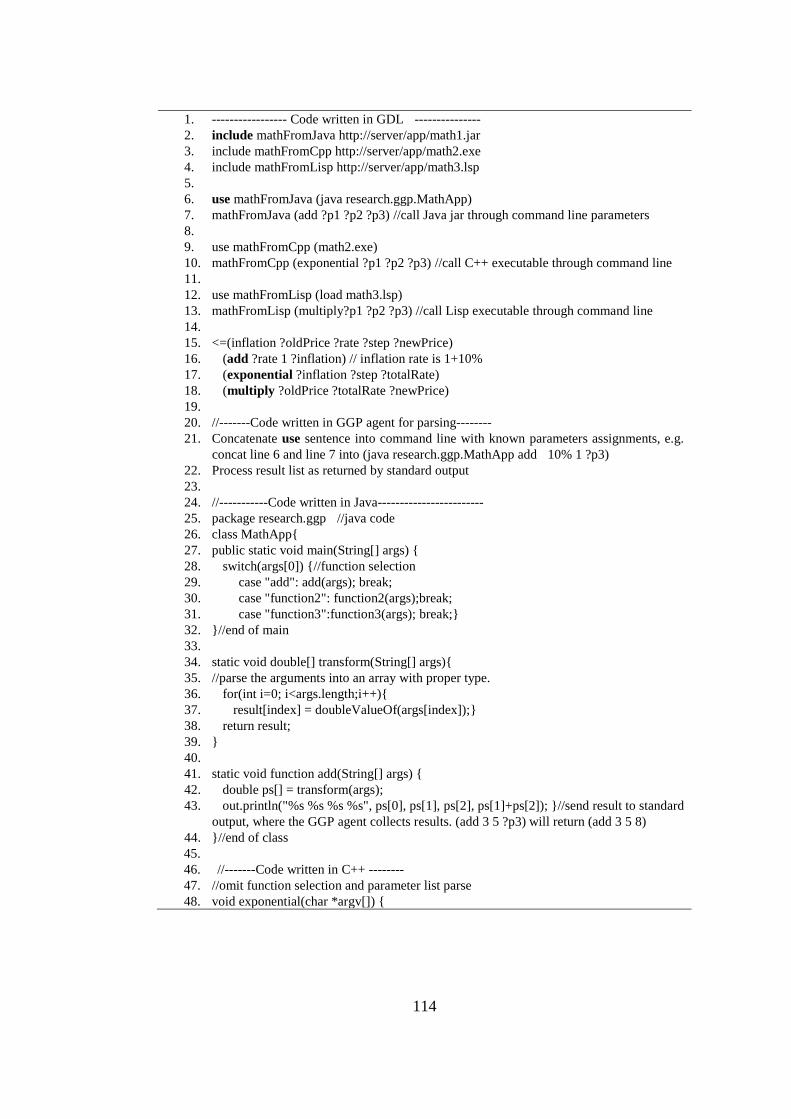
114

1. ----------------- Code written in GDL ---------------

2. include mathFromJava http://server/app/math1.jar

3. include mathFromCpp http://server/app/math2.exe

4. include mathFromLisp http://server/app/math3.lsp

5.

6. use mathFromJava (java research.ggp.MathApp)

7. mathFromJava (add ?p1 ?p2 ?p3) //call Java jar through command line parameters

8.

9. use mathFromCpp (math2.exe)

10. mathFromCpp (exponential ?p1 ?p2 ?p3) //call C++ executable through command line

11.

12. use mathFromLisp (load math3.lsp)

13. mathFromLisp (multiply?p1 ?p2 ?p3) //call Lisp executable through command line

14.

15. <=(inflation ?oldPrice ?rate ?step ?newPrice)

16. (add ?rate 1 ?inflation) // inflation rate is 1+10%

17. (exponential ?inflation ?step ?totalRate)

18. (multiply ?oldPrice ?totalRate ?newPrice)

19.

20. //-------Code written in GGP agent for parsing--------

21. Concatenate use sentence into command line with known parameters assignments, e.g.

concat line 6 and line 7 into (java research.ggp.MathApp add 10% 1 ?p3)

22. Process result list as returned by standard output

23.

24. //-----------Code written in Java------------------------

25. package research.ggp //java code

26. class MathApp{

27. public static void main(String[] args) {

28. switch(args[0]) {//function selection

29. case "add": add(args); break;

30. case "function2": function2(args);break;

31. case "function3":function3(args); break;}

32. }//end of main

33.

34. static void double[] transform(String[] args){

35. //parse the arguments into an array with proper type.

36. for(int i=0; i<args.length;i++){

37. result[index] = doubleValueOf(args[index]);}

38. return result;

39. }

40.

41. static void function add(String[] args) {

42. double ps[] = transform(args);

43. out.println("%s %s %s %s", ps[0], ps[1], ps[2], ps[1]+ps[2]); }//send result to standard

output, where the GGP agent collects results. (add 3 5 ?p3) will return (add 3 5 8)

44. }//end of class

45.

46. //-------Code written in C++ --------

47. //omit function selection and parameter list parse

48. void exponential(char *argv[]) {

115

49. double ps[] = transform(char *argv[]);

50. cout <<ps[0]<<" "<<ps[1]<<" "<<ps[2]<<" " ps[1]^ps[2] << endl; }

51.

52. //-------Code written in Lisp--------

53. //omit function selection and parameter list parse

54. (defun multiply(args)

55. (setq result (* (second args) (third args)))

56. (remove '?p3 args)

57. (append args (list result)))

116

The pseudo-code shows a straightforward example of how to include and use the

external resources in different computer languages. The GDL code (lines 1-19) is

available to all players. The executables of different languages are available at some

public URL for all players too. Depending on the programming languages that the

GGP agents use, the agent needs to add additional keyword parsing ability to parse

include and use, just as it parses other keywords. The GDL code needs to be parsed

into a command line to call the public executables with parameters (line 21). The

parsing process assigns values to known parameters, and concatenates them into a

command line to call the target executables. The parsing schema is independent of the

language in which the GGP agent is written or the language in which the executable is

written. The agent collects standard output as the results returned (line 22). When

calling the executables, not all parameters need to be instantiated (e.g. line 21). The

undecided parameters' value will be filled by the external calculation. When there are

multiple assignments of the parameters, the external functions can be called multiple

times, each time with one assignment list.

Instead of defining the numbers, the number sequence, and number addition as in

Figure 7.1, the add function is not defined in the game rules. GDL uses the include

keyword to refer to a foreign resource and pass three parameters (two instantiated)

117

with the use keyword. The same calculation that took O(n 2

) time in Figure 7.1 can

be done in O(1) time now.

The foreign resource can be a shared file, a URL, or a database library. It is accessible

by all players. The foreign data structure can be a list of facts, functions, or

calculations. We have tested Java, C++ and Lisp. The same experiments can easily be

done in other programming language(s) as well. The area of specific knowledge can

be game related such as resource utilization or, more generally, eCommerce or a

social scenario.

Note that the GGP agent does not need a corresponding compiler to invoke the

executables. Only the running environment for the executables needs to be set up, just

like .exe on Windows, or bash on Linux. Additional steps need to be taken for cross

platform implementation such as data transfer from Windows to Linux, or to Mac, etc.

In the future, the executable invoking process can be generalized into a more

universal solution such as using web services or cloud computing.

To summarize, as long as the parameters can be passed back and forth through the

information façade, the game functions can perform the query to complete the logic

resolution. Where the data are stored and how the data are organized are not GDL's

concern any more.

118

7.3 Impact of the Extension

The modifications and extensions of GDL broaden the GGP area and raise the set of

potential applications to a new level. GDL is sufficiently expressive to model many

relations. However, the fact that GDL is capable of describing many real world

scenarios does not mean it can be done in a concise or effective manner and it

certainly does not help or force the game designer to do so in a reasonable manner.

Section 7.1.1 is an example of a tedious definition of a small group of natural numbers

and addition operations. When it comes to the game goal determination or infinite real

number calculations, the existing GDL structure is hindering rather than enabling new

games being brought to the general game playing field. Since there exist arithmetic

libraries described in other computer programming languages, redefining everything

again in GDL not only adds little values to the GGP system, but also is discouraging

people from turning to the GGP system for problem solving. The include and use

keyword would introduce the arithmetic library and thereby make additional games

possible in the GGP. With the new keywords include and use available to open the

interface with other languages, existing information or data from other domains can

be easily hooked to the GGP engine.

119

7.4 Extension Application to Coalition Games

The external information provided via the include and use keywords is used only for

the knowledge resolution and reasoning process within the game description.

Different game agents are given the same game to play; therefore the same external

functions to use. The logic resolution performance will be improved in a way that

shifts from "how the game is written" to "what the game is about.” But the decision

making and agents’ performance are still completely determined by the game playing

algorithms.

At the beginning of the Section 7.2, we mentioned that the GDL extension would

benefit market-trading economic and incomplete information games. Coalition games

are another important area of game playing research that would benefit from the GDL

extension.

7.4.1 Coalition Games

A coalition game with transferable utility is defined as (N, v), where N is finite set of

players; v : 2N→ R associates with each subset S⊆ N a real-valued payoff v(S)

(Leyton-Brown, 2008). The inherent payoff calculations in coalition games strongly

motivated and essentially required that the calculations be defined in the GDL

extension rather than directly in GDL.

120

There have been multi-player games that require playing in groups in the GGP area.

The six-player 3D Tic-Tac-Toe (see reference Tic-Tac-Toe 3D 6-player) requires

players to play in groups of three. Each player picks the coordinate value in one

dimension. The three dimensions picked by the three players determine the final

position of the piece. The four player Othello (see reference Othello 4-player) game is

similar. Four players are divided in groups of two, with each player picking one

coordinate. Unlike these two games that are played in groups, coalition games require

that each agent can play the games both by itself and in groups. There have not been

any published coalition games in GGP.

The extension of GDL makes describing coalition games possible. Using the extended

GDL, we can explore more realistic economic and societal problems. The focus of

this section is not a study of the coalition games as such, but an example of the use of

the GDL extension in coalition games. The results show our extensions generated

reasonable results for an eCommerce coalition game.

7.4.2 Coalition Farmer Game

The Farmer game contains a simplified skeleton of manufacturer financial activities

and elements of the stock market (see Section 3.4). The Farmer game opens the

121

possibility of using the general game playing techniques to explore and perhaps even

solve skeletal real world financial or social problems.

The current Farmer game is defined as a win-or-lose game. The player that ended up

with the most money at the end of the game wins with 100 points awarded. If the

player owns the same amount of money as another player, or less money than another

player, he loses with zero points awarded.

However, the nature of the Farmer game is indeed an eCommerce game with financial

achievements. In a more realistic scenario, when three players started with the same

amount of money and face the same market rules, they do not have to become the

richest among the three to be rewarded. The amount of money the player owns is the

real reward. How much the player earned during the process matters. The player

would be happier with 100 gold pieces and finishing in second place, than with 60

gold pieces and finishing in the first place. The metrics of winning is different in

reality.

In addition to the amount of gold pieces earned, the three players can be more

cooperative than competitive. In the open market setting with a fixed inflation number,

buying a small amount in each step, holding till the end of the game, then selling

together at the last step can be an easy solution for all three players to get rich. This is

because pushing the price high every step with a purchase action benefits all players.

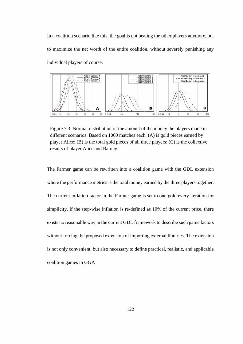
122

In a coalition scenario like this, the goal is not beating the other players anymore, but

to maximize the net worth of the entire coalition, without severely punishing any

individual players of course.

The Farmer game can be rewritten into a coalition game with the GDL extension

where the performance metrics is the total money earned by the three players together.

The current inflation factor in the Farmer game is set to one gold every iteration for

simplicity. If the step-wise inflation is re-defined as 10% of the current price, there

exists no reasonable way in the current GDL framework to describe such game factors

without forcing the proposed extension of importing external libraries. The extension

is not only convenient, but also necessary to define practical, realistic, and applicable

coalition games in GGP.

Figure 7.3: Normal distribution of the amount of the money the players made in

different scenarios. Based on 1000 matches each. (A) is gold pieces earned by

player Alice; (B) is the total gold pieces of all three players; (C) is the collective

results of player Alice and Barney.

123

With the extension of GDL, we added the gold pieces from each of the players to get

the total gold pieces earned by the three players for a coalition game. When each of

the three players is trying to make their own best net worth (individually and

collectively), the total value of the game (number of gold pieces as presented on the

X-axis in Figure 7.3) increases with more cooperation.

We analyzed four experimental scenarios of the Farmer game with 1000 simulations

each. In Scenario 1, an intelligent GGP agent Alice plays against random dummy

players Barney and Charlie. Alice is using the contextual decision trees. Alice earns

almost twice as much as Barney or Charlie that shows the value of the intelligent

agent. In Scenario 2, both Alice and Barney are using intelligent decision making for

actions while Charlie remains a random player. Here both Alice and Barney earn

twice as much as Charlie and Alice increases her earning over her earnings in

Scenario 1. Scenario 3 has all three players using intelligent agents to make

strategic decisions to maximize their individual income. In Scenario 3 both Alice

and Barney improve their earnings over Scenarios 1 and 2 where they were the only

one or two, respectively, trying to optimize their earnings. Scenario 4 has Alice

and Barney in a coalition playing against the intelligent player Charlie. Compared to

the Scenario 3, Alice and Barney both focus on maximizing the sum of their

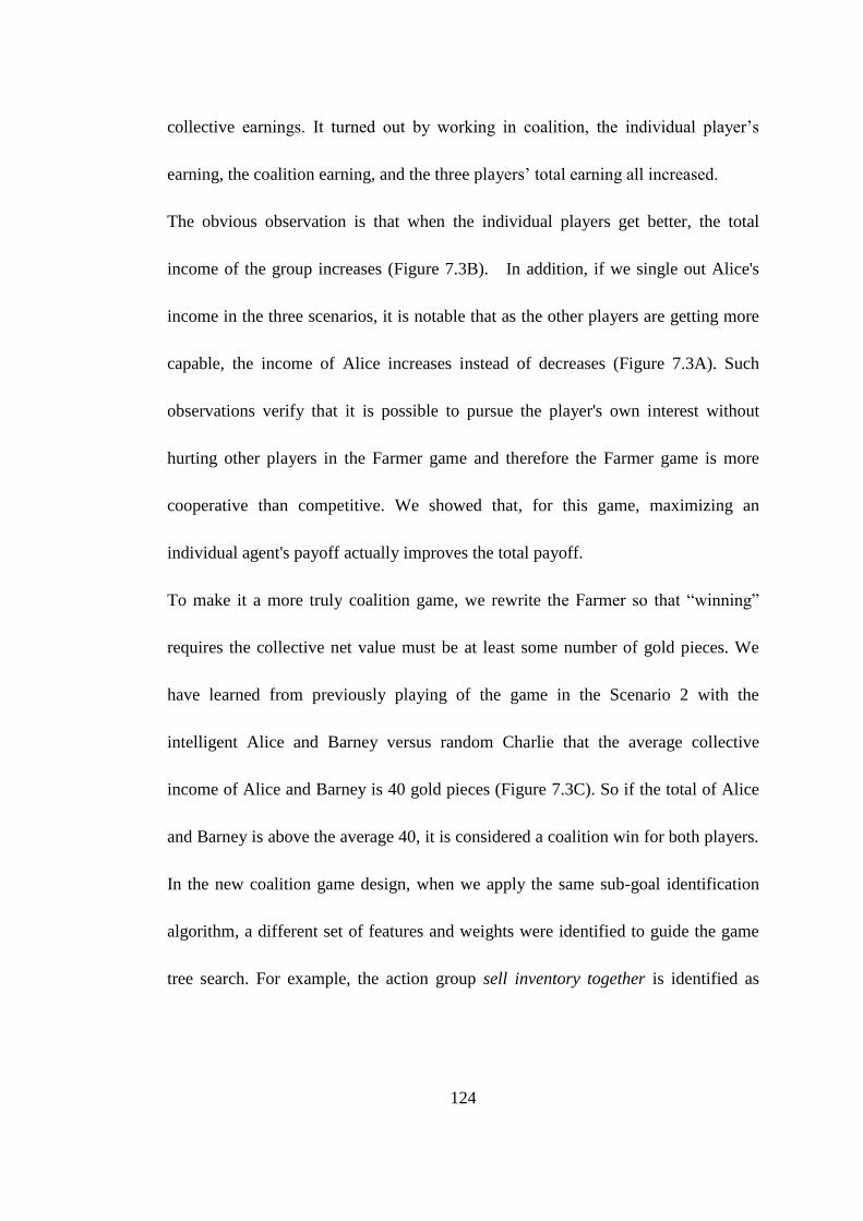
124

collective earnings. It turned out by working in coalition, the individual player’s

earning, the coalition earning, and the three players’ total earning all increased.

The obvious observation is that when the individual players get better, the total

income of the group increases (Figure 7.3B). In addition, if we single out Alice's

income in the three scenarios, it is notable that as the other players are getting more

capable, the income of Alice increases instead of decreases (Figure 7.3A). Such

observations verify that it is possible to pursue the player's own interest without

hurting other players in the Farmer game and therefore the Farmer game is more

cooperative than competitive. We showed that, for this game, maximizing an

individual agent's payoff actually improves the total payoff.

To make it a more truly coalition game, we rewrite the Farmer so that “winning”

requires the collective net value must be at least some number of gold pieces. We

have learned from previously playing of the game in the Scenario 2 with the

intelligent Alice and Barney versus random Charlie that the average collective

income of Alice and Barney is 40 gold pieces (Figure 7.3C). So if the total of Alice

and Barney is above the average 40, it is considered a coalition win for both players.

In the new coalition game design, when we apply the same sub-goal identification

algorithm, a different set of features and weights were identified to guide the game

tree search. For example, the action group sell inventory together is identified as

125

important, because the price drops after each selling action so the inventory is

devalued by another player's selling action. When Alice and Barney are cooperating

in Scenario 4, the coalition income exceeded the addition of the individual income in

Scenario 3.

To summarize, the GDL extension enables complex payoff distributions and

therefore allows the new coalition version of the Farmer game, in which each of the

three or more players can have their own strategy or a group strategy. The players can

play individually to determine how much they can win, or in coalition with the

definition of winning for the game being the collective winnings of any given

coalition. Scenario 4 in Figure 7.3C gives the results of Alice and Barney coalition

when they are actively cooperating to maximize the sum of their winnings. Scenario 4

provides the highest winnings for any of the examined renditions of the 10 iteration

Farmer game. The collective achievements do not necessarily conflict with

individual payoffs. Depending on the games rules, there exist situations where

maximizing collective payoffs would strengthen individual payoffs and vice versa.

7.5 Benefits and Concerns

Since the emergence of the GGP area, the focus of the research has been on how to

build a good agent. Yet this chapter discusses how to incorporate more GGP games

126

into the GGP research. The GDL extension opens the door for extending the GGP

into new, realistic, coalition eCommerce applications. The coalition Farmer game is

an example of using the modifications and extensions of GDL. The coalition games

broaden the GGP research area as we study how the dynamics change from

competitive to coalition games. Fresh insights will be gained in both the specific

games and GGP.

In GGP games, the logic knowledge can be divided into static information that does

not change from the beginning to the end of the game (e.g. the board adjacency) and

dynamic information that changes from step to step. With the GDL extension,

theoretically, only game elements such as the game state, player's role, goals, state

transition, legal actions, etc. need to be defined in GDL and all other computational

intensive functions can be imported from or defined in the user’s favorite languages.

However, the time spent passing parameters back and forth is considered game time

cost as well. Most static information can be defined outside GDL with the expectation

of improving performance since the parameters are only passed once. The arithmetic

calculations that have extremely high cost within GDL should be defined outside

GDL. The minor or moderate calculation that demand frequent changes as the game

state changes need to handled with caution. It is up to the game writers’ judgment to

determine if keeping the function definition in or outside GDL is more efficient.

127

It is possible that certain GGP agents in the field today will be affected by the

extension and lose their advantage in competitions. In fact, the annual GGP

competition does not have to implement the proposed extension, as long as the

researchers do not mind writing every new game with GDL for the competition. But

the GDL extension proposed in this dissertation allows people to contribute to the

GGP area without being experts in GDL. Therefore, it would give agents access to

more games outside of GDL and hence attract more people into the GGP area in the

long run. As GGP agents become more powerful and with this GDL extension, GGP

agents may contribute to solutions in diverse domains.

The purpose of extending GDL goes beyond number calculation and even beyond

introducing coalition games. It is the first step of setting up a system in which an

existing game written in other programming languages does not need to be completely

rewritten into GDL to let the GGP agent play. We believe as long as the basic game

elements such as initial state, player's role, legality, state transition, and goals are

re-defined in GDL, a new game can be added to the GGP family without importing

the data relations, computations, and storage.

128

8 Summary

In summary, we presented five pieces of research contributions: the general game

playing agent that plays a wide variety of games, the knowledge reasoning algorithm

to improve the agent's performance, the run-time feature identification algorithm to

dynamically analyze winning features in different games, the automated decision

making algorithm based on the game context, and the GDL extension to enrich games

allowed in the GGP domain. Each contribution has been published.

Creating a general game playing agent that does not assume any specific game

elements (such as boards or pieces), but plays solely based on the logic relations in a

given game attacks the general intelligence problem which is appealing to many AI

researchers. The games we discussed in this dissertation provide examples for our

explanations. The GDL definition limits the games to "finite, discrete, deterministic

complete information games" to simplify the problem for early progress (Love, 2005).

But new game categories have been added to GDL to expand the research scope.

There are limitations on the kind of games that our agent can effectively learn in order

to improve playing performance. Because the useful learning data are gathered only

from random playing of games that end in a win and games like Chess or Go seldom

terminate during random play, it is practically impossible to collect a large enough

129

training set for data analysis for these games. Theoretically, our game agent is able to

improve in almost all cases that it is able to get an effective training set. Farmer, with

the branching factor of 1000, is a good example showing our learning agent can play

and improve performance in complicated games, although the playing result is still far

from being optimal.

In addition to our decision tree learning algorithm, there are three other learning

algorithms in the GGP field. Each has certain limitations of not being effective on

certain kinds of games because of the inherent design of its learning (Section 3.2). Our

decision tree learning algorithm has practical concerns to play certain games, but does

not have inherent design barriers; i.e. given enough resources to gather a large enough

training set, it can play any game written in GDL. We also discussed other attempts to

improve the learning algorithms such as active learning or reinforcement learning.

These attempts sacrifice the generality in exchange for efficiency (Section 5.1). That

diverts from the focus of our GGP research.

130

9 Future Work

The general game playing attacks the general intelligence problem on which AI

researcher have found difficult to make progress for the last several decades. It

includes comprehensive AI topics like knowledge reasoning, planning, search and

learning. Although GGP has drawn considerable attention and has developed

vigorously over the last few years, this area is still in its infancy.

9.1 GGP Definition

Because strategic game playing has been a computer science exercise with relatively

few real world applications, it is natural to consider GGP as a more advanced layer of

game playing on the same academia level. But GGP has a potential to develop into a

general problem analyst and a general problem solver. We understand game play as

an instant reward system where people can get timely feedback for actions taken. By

introducing more games into this framework, the players may become capable of

solving real problems. The GDL extension proposed in Chapter 7 is an important step

to add new game categories to the area. We plan to investigate other coalition games

and formalize GDL extension with more examples. We would like to extend the

131

eCommerce game to four players with two players in each coalition, use multiple

units of commodity inventory and utility transfer to test how the GGP agent will work.

At the beginning of GGP (2005), the games were limited to "finite, discrete,

deterministic complete information games" to simplify the problem for early progress

(Love, 2005). In the recent workshops, many researchers have agreed arithmetic must

be part of the GGP. Beyond that, different areas may need different elements for

domain specific problems. The existing game agents need to evolve as the game

specification moves forward. Certain techniques such as rule analysis or tree search

may not apply to new general physics games or new general video games. Broadening

the scope of general game playing, designing a broader problem specification

language, and building agents capable of solving general problems in different

categories, is very interesting and a natural next step.

9.2 GGP Competition

In the GGP competition set-up, agents are given minutes for game preparation and

seconds for each step. Such game playing configurations make it very difficult for

learning algorithms to gather enough training data from which to learn. That is one

reason GGP research has primarily focused on search improvements rather than

learning improvements.

132

To encourage research in GGP machine learning, the annual GGP competition at

AAAI and IJCAI is considering splitting into different tracks in the future. In the 2011

IJCAI workshop on general game playing, Nathan Sturtevant, Michael Thielscher,

Daniel Michulke and I discussed changing the competition configuration so that

players specialized in learning can compete. We agreed that minutes or even hours of

game preparation time is too short for agents to collect meaningful data from which to

learn. The agent specializing in learning should be given weeks or months of game

preparation time to play against other players specializing in learning. The first

attempt for a separate track designed for the GDL extension to incorporate

non-deterministic, incomplete information games was held in Germany in October,

2011.

Selecting games for the GGP competition is another challenge. It is not surprising to

see agents that are good at some games but not good at others. Recent competitions

last less than a week. If a player encounters a bad game type, it will be dropped out of

the competition early. It may be better to have the GGP agents compete in a

tournament rather than a single elimination but with head-to-head competition in the

final round.

133

9.3 GGP Evaluation

The GGP agent is a complicated project with many components (search, planning,

learning, etc.) involved. When the player wins (or loses), it is very difficult to measure

which piece of the agent worked (or failed). Evaluating the contribution of different

GGP components is not addressed in the current literature.

We propose creating dummy player skeletons into which different components can

plug-and-play. With a new defined interface and communication protocol, a new

component can be singled out and plugged into the dummy skeleton to play. All the

performance changes before and after the component replacement can be measured

and evaluated. This encourages new people to enter this area by lowering the

threshold from building one complete agent to building and evaluating one

component.

Because of the lack of evaluation criteria for the GGP configurations, we created our

own measurements in several situations (see Section 4.4, 5.4, 6.2.5, 5.3.3). Such

measurements provided insights on how the algorithms improve the agents, but

allocating time resources between learning and search was not explored. Monte-Carlo

tree search has been the best GGP search algorithm so far, searching up to 1,000,000

nodes per move (Finnsson, 2011). We talked to Hilmar Finnsson about combining

their searching and our learning algorithms into one agent. It should be very

134

interesting to investigate how the resource allocation between learning and search

would change as game dynamics change. Our hypothesis is that for small games,

search can use the time better than learning, but for large games with enormous search

space, the time spend on learning will be better invested.

In addition to the statistical feature identification algorithm, we are investigating

using genetic algorithms for state evaluations. Preliminary research appears

promising.

As the general game playing research matures, the game scope will be extended. The

competition configuration will be improved and may be extended to separate

competitions for search algorithms, learning algorithms, and games in different

domains. This will allow better evaluation measurements of the various GGP

components and more rapid improvements in GGP and therefore advance the entire

field. General game playing is a sophisticated area with huge potential.

135

REFERENCES

Allis, V. (1988). "A Knowledge-based Approach of Connect-Four, The Game is

Solved: White Wins", Master's thesis, University Amsterdam, Netherlands.

Angelides, M., and R. Paul (1993). “Towards a Framework for Integrating Intelligent

Tutoring Systems and Gaming Simulation”, in Proceedings of the 25th Conference on

Winter Simulation, 431-443, Los Angeles, CA.

Banerjee, B., and P. Stone (2007). "General Game Learning Using Knowledge

Transfer", in Proceedings of the International Joint Conference on Artificial

Intelligence (IJCAI), 672-677, Hyderabad, India.

Billings, D., A. Davidson, J. Schaeffer, and D. Szafron (2002). "The challenge of

poker", Artificial Intelligence, 134(1–2), 201–240.

Bjornsson, Y., and H. Finnsson (2009). "Cadiaplayer: A simulation-based general

game player", IEEE Transactions on Computational Intelligence and AI in Games,

1(1), 4–15.

Brachman, R. and H. Levesque (2004). Knowledge Representation and Reasoning,

Morgan Kaufmann, San Francisco.

Bramer, M. (2007). Principles of data mining, 119-134, Springer, New York.

Buro, M. (1997). "The Othello match of the year: Takeshi Murakami vs. Logistello",

Journal of International Computer Chess Association, 20(3), 189–193.

Clune, J. (2007). "Heuristic evaluation functions for general game playing", in

Proceedings of the 22nd AAAI Conference on Artificial Intelligence, 1134-1139,

Vancouver, Canada.

Cox, E., E. Schkufza, R. Madsen, and M. Genesereth (2009). "Factoring general

games using propositional automata", in Proceedings of the IJCAI Workshop on

General Intelligence in Game-Playing Agents (GIGA), 13-20, Pasadena.

De Groot, A.D. (1965). Thought and Choice in Chess, Amsterdam University Press,

Amsterdam, Netherlands.

136

Edelkamp, S., and P. Kissmann (2011). "On the Complexity of BDDs for State Space

Search: A Case Study in Connect Four", in Proceedings of the IJCAI Workshop on

General Intelligence in Game-Playing Agents, 15-21, Barcelona, Spain.

Finnsson, H., and Y. Bjornsson (2009). "Simulation-based approach to general game

playing", in Proceedings of the 23rd AAAI Conference on Artificial Intelligence,

259–264, Chicago.

Finnsson, H. and Y. Bjornsson (2010). "Learning simulation control in general

game-playing agents", in Proceedings of the AAAI Conference on Artificial

Intelligence, 954-959, Atlanta.

Finnsson, H. and Y. Bjornsson (2011). "Game-Tree Properties and MCTS

Performance", in Proceedings of the IJCAI Workshop on General Intelligence in

Game-Playing Agents, 23-30, Barcelona, Spain.

Genesereth, M. and R. Fikes (1992). Knowledge Interchange Format, Version 3.0.

Reference Manual, Logic Group Report Logic-92-1, Computer Science Department,

Stanford, CA.

Genesereth, M. and N. Love (2005). "General Game Playing: Overview of the

AAAI Competition", AI Magazine, 26(2), 62–72.

GGP Dresden. http://www.general-game-playing.de

GGP player: http://www.general-game-playing.de/downloads.html.

GGP Stanford. http://games.stanford.edu/

Gudmundsson, S. F. and Y. Bjornsson (2011). "MCTS: Improved Action Selection

Techniques for Deterministic Games", in Proceedings of the IJCAI Workshop on

General Intelligence in Game-Playing Agents, 45-52, Barcelona, Spain.

Hsu, F.-H. (2002). Behind Deep Blue: building the computer that defeated the world

chess champion, Princeton University Press, Princeton, NJ.

137

Kaiser, L. and L. Stafiniak (2011). "First-order logic with counting for general game

playing", in Proceedings of the AAAI Conference on Artificial Intelligence, San

Francisco.

Kirci, M., N. Sturtevant and J. Schaeffer (2011). "A GGP feature learning

algorithm", KI - Künstliche Intelligenz, 25(1), 35-42.

Kissmann, P. and S. Edelkamp (2011). "Gamer, a general game playing agent", KI -

Künstliche Intelligenz, 25(1), 49-52.

Korf, R. (1985). "Depth-first iterative-deepening: An optimal admissible tree

search", Artificial Intelligence, 27(1), 97–109.

Kostenko, A. (2007). Calculating End Game Databases for General Game Playing,

Master thesis, Dresden University of Technology, Germany.

Kroeker, K. (2011). “A new benchmark for artificial Intelligence”, Communications

of the ACM, 54(8), 13-15.

Kuhlmann, G. and P. Stone (2006). “Automatic Heuristic Construction in a

Complete General Game Player", in Proceedings of the 21st AAAI Conference on

Artificial Intelligence, 1457–1462, Boston, MA.

Kuhlmann, G. and P. Stone (2007). "Graph-Based Domain Mapping for Transfer

Learning in General Games", in Proceedings of the Eighteenth European

Conference on Machine Learning, 188-200, Warsaw, Poland.

Leyton-Brown, K., and Y. Shoham (2008). Essentials of Game Theory, Morgan and

Claypool Publishers.

Love, N., T. Hinrichs, D. Haley, E. Schkufza, and M. Genesereth (2005). General

Game Playing: Game Description Language Specification, Technical report,

Computer Science Department, Stanford University, Stanford, CA.

Méhat, J., and T. Cazenave (2010). "Combining UCT and nested monte-carlo search

for single-player general game playing", IEEE Transactions on Computational

Intelligence and AI in Games, 2(4), 271–277.

138

Méhat, J. and T. Cazenave (2011), "A Parallel General Game Player", KI -

Künstliche Intelligenz, 25(1), 43-47.

Mingers, J. (1989), "An Empirical Comparison of Pruning Methods for Decision

Tree Induction", Machine Learning, 4(2), 227-243.

Michulke, D. and M. Thielscher (2009). "Neural networks for state evaluation in

general game playing", in Proceedings of the European Conference on Machine

Learning (ECML), 95-110, Bled, Slovenia.

Michulke, D. (2011). "Neural Networks for High-Resolution State Evaluation in

General Game Playing", in Proceedings of the IJCAI Workshop on General

Intelligence in Game-Playing Agents, 31-38, Barcelona, Spain.

Möller, M., M. Schneider, M. Wegner, and T. Schaub (2011). "Centurio, a General

Game Player: Parallel, Java- and ASP-based", KI - Künstliche Intelligenz, 25(1),

17-24.

Othello 4-player. http://euklid.inf.tu-dresden.de:8180/ggpserver/public/view_game.

jsp?name=othello-fourway

Pell, B. (1993). Strategy Generation and Evaluation for Meta-Game Playing, PhD

thesis, University of Cambridge, United Kingdom.

Quinlan, J. (1986). "Induction of Decision trees", Machine Learning, 1(1), 81-106.

Quinlan, J. (1993), C4.5: Programs for Machine Learning, Morgan Kaufmann

Publishers, San Mateo.

Russell S.J., P. Norvig (2003). Artificial Intelligence: A Modern Approach (2nd ed.),

221-277, Prentice Hall, NJ.

Saffidine, A. and T. Cazenave (2011). "A forward chaining based game description

language compiler", in Proceedings of the IJCAI Workshop on General Intelligence

in Game-Playing Agents (GIGA), 69-75, Barcelona, Spain.

139

Schaeffer, J. (1997). One Jump Ahead: Challenging Human Supremacy in Checkers,

Springer, Berlin.

Schaffer, C. (1993). "Overfitting Avoidance as Bias", Machine Learning, 10(2),

153-178, MA.

Schkufza, E., N. Love, and M. Genesereth (2008). "Propositional automata and cell

automata: Representational frameworks for discrete dynamic systems", in

Proceedings of the Australian Joint Conference on Artificial Intelligence, 56-66,

Auckland, Australian.

Schiffel, S. and M. Thielscher (2007). "Fluxplayer: a successful general game

player", in Proceedings of the 22nd AAAI Conference on Artificial Intelligence,

1191–1196, Vancouver, Canada.

Schiffel, S. and M. Thielscher (2009a). "A Multiagent Semantics for the Game

Description Language", in Proceedings of the International Conference on Agents

and Artificial Intelligence, Porto, Portugal.

Schiffel, S. and M. Thielscher (2009b). "Automated theorem proving for general

game playing", in Proceedings of the International Joint Conference on Artificial

Intelligence (IJCAI), 911-916, Pasadena.

Sheng, X. and D. Thuente (2010a). "Predicative Sub-goal Analysis in a General Game

Playing Agent", in Proceedings of International Conference on Web Intelligence and

Intelligent Agent Technology, 423-427, Toronto, Canada.

Sheng, X. and D. Thuente (2010b). "Using Hash Tables to Expedite Knowledge

Reasoning in the General Game Playing Agent", in Proceedings of International

Conference on Advanced Topics in Artificial Intelligence, 91-96, Thailand, 2010.

Sheng, X. and D. Thuente (2011a). "Using Decision Trees for State Evaluation in

General Game Playing", KI - Künstliche Intelligenz, 25(1), 53-56.

Sheng, X. and D. Thuente (2011b). "Decision Tree Learning in General Game

Playing", in Proceedings of Artificial Intelligence and Applications, 192-199,

Innsbruck, Austria, 2011.

140

Sheng, X. and D. Thuente (2011c). “Extending the General Game Playing Framework

to Other Programming Languages”, in Proceedings of International Conference on

Artificial Intelligence, Las Vegas, Nevada.

Sheng, X. and D. Thuente (2011d). "Contextual Decision Making in General Game

Playing", in Proceedings of 23rd IEEE International Conference on Tools with

Artificial Intelligence, 679-684, Boca Raton, Florida.

Sheng, X. and D. Thuente (2011e). “Extending the General Game Playing Framework

to Other Programming Languages”, in Proceedings of the IJCAI Workshop on

General Intelligence in Game-Playing Agents (GIGA), 77-84, Barcelona, Spain.

Tesauro, G. (1992). "Practical issues in temporal difference learning", Machine

Learning, 8(3-4), 257–277.

Thielscher, M. (2009a). "Answer set programming for single-player games in

general game playing", in Proceedings of the International Conference on Logic

Programming, 327-341, Pasadena.

Thielscher, M., and D. Zhang (2009b). "From General Game Descriptions to a

Market Specification Language for General Trading Agents", Workshop on Trading

Agent Design and Analysis.

Thielscher, M. (2010). "A General Game Description Language for Incomplete

Information Games ", in Proceedings of the 24th AAAI Conference on Artificial

Intelligence, 994-999, Atlanta.

Tic-Tac-Toe 3D 6-player. http://euklid.inf.tu-dresden.de:8180/ggpserver/public/

view_game.jsp?name=tictactoe_3d_6player

Turing, A. (1950), “Computing Machinery and Intelligence,” Mind, 49(236),

433–60.

Wackerly, D., W. Mendenhall and R. Scheaffer (2008). Mathematical Statistics with

Applications, 7th edition, Cengage Learning.

141

Waugh, K. (2009). "Faster state manipulation in general game playing using

generated code", in Proceedings of the IJCAI Workshop on General Intelligence in

Game-Playing Agents (GIGA), 91-97, Pasadena.

142

APPENDICES

143

APPENDIX A

General Game Playing Example Game List

1. Blocks: Move three bricks around so that they are line up vertically.

2. Buttons: Three buttons (a, b, c) and three lights (p, q, r). Press the buttons to turn

all lights on.

3. Endgame: White king and rook against black king on regular Chess board. White

must checkmate within 16 moves (Figure 3.3D).

4. Maze: The maze contains four interconnected cells. Robot is in A and Gold in C.

The robot can move, grab, or drop. The goal is to get the gold to the beginning cell A

(Figure 3.3A).

5. Mini-Chess: Small size Chess on a 4 by 4 board. White with one king and one rook

play against Black king. White must checkmate within ten steps to win (Figure 3.4A).

6. Rock-paper-scissors: Roshambo is another name for Rock, Paper, Scissors. Also

known as Scissors, Paper, Stone. A game of randomness.

7. Tic-tac-toe: Try to line three Xs or three Os. (Figure 3.3B).

8. Simultaneous Tictactoe: Both players go at the same time. If both tried to mark the

same cell, the cell remains empty.

144

General Game Playing Example Game List

9. Chess: regular Chess

10. Blocker: Simultaneous game on a 4 by 4 board. One player is trying to block the

other player from creating a path from the left to right.

11. Connect Four: Classic Connect Four on 6 by 7 board for White and Black players

to line up four pieces (Figure 3.4B).

12. Farmer: Three players move simultaneously, trying to make money by buying and

selling farms, factories, and commodities (Figure 3.4D).

13. Eight-puzzle: Single-player eight-puzzle game. The player slide blocks (tiles) to

get all the numbers to their correct positions.

14. Simultaneous Wall-maze: A maze game in which players make simultaneous

moves. If the moves collide, all players stay where they were.

15. Guess: One player tries to guess a number, the other responds higher or lower

accordingly. The responder may change his number, as long as the new number is

consistent with his earlier responses.

16. Tetris: A move-based Tetris with no piece rotation. The player tries to line up the

pieces into lines.

145

General Game Playing Example Game List

17. Connect Four variation: Connect Four on eight by eight horizontal board. Players

can put his pieces on any place of the board.

18. Othello: it is also called Reversi. Players can flip the opponent's pieces. The player

with more pieces on the board at the end of the game wins (Figure 3.4C).

19. Pancake: The player is a cook at a short order diner, and wants to flip pancakes

into the shape of a pyramid.

20. Nothello: The opposite of Othello. The players with less pieces on the board wins.

The board is changed with corners cut off.

21. Peg Jumping: Every peg jump removes a peg. The goal is to remove all pegs, but

leave one in the center.

22. Chinese Checkers variation 1: Small Chinese Checkers with one player.

23. Crossing Chinese Checkers: A simplified version of Chinese Checkers (Figure

3.3C).

24. Three-player Checkers: three players trying to move or jump to the other end of

the Checkers board.

146

General Game Playing Example Game List

25. Circles Solitaire: remove all circles on a board (graph).

26. Hallway walking: The board is a simplified corridor with only horizontal walls.

Players walk across the board to the other end.

27. Racetrack: A simultaneous-play corridor variation. The goal is to place walls to

impede the opponent in a race to the end.

28. Queens: Eight-Queens problem on Chess board.

29. Four-player Othello: Four players divided in two groups. Each picks one

coordination for the Othello move.

30. 3D Tic-Tac-Toe: Six players divided in two groups. Each picks one coordination

for the 3D Tic-Tac-Toe move.

31. Breakthrough: Two players begin with 16 pieces each on a eight by eight board,

trying to reach the other side of the board while blocking the opponent.

32. Hanoi: Towers of Hanoi

33. Catch me if you can: three players on seven by seven board. If one player catches

the other, he gets one point. The game ends in 31 steps and the highest score wins the

game.

147

General Game Playing Example Game List

34. Two-player normal form: The three by three version of prisoner's dilemma. Two

players make simultaneous moves. One pick the horizontal value, the other pick the

vertical value.

35. Beat Mania: a revision of Tetris. The dropper drops items from the top of a 30 by

three well for 30 times, the catcher scores for every successful catch.

36. Coins: Single-player game. The board has eight cells. Each cell has a coin in it.

The player moves the coins around, or jumps over the coins.

37. Six-player Checkers.

38. Double Tic-Tac-Toe: players move alternatively on two boards.

39. Fire fighter: Fire changes the maze layout.

40. Farmer with 20 iterations.

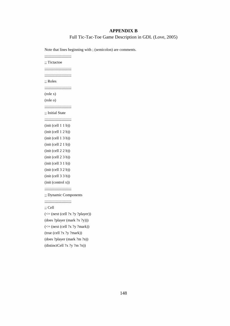
148

APPENDIX B

Full Tic-Tac-Toe Game Description in GDL (Love, 2005)

Note that lines beginning with ; (semicolon) are comments.

;;;;;;;;;;;;;;;;;;;;;;;;;

;; Tictactoe

;;;;;;;;;;;;;;;;;;;;;;;;;

;;;;;;;;;;;;;;;;;;;;;;;;;

;; Roles

;;;;;;;;;;;;;;;;;;;;;;;;;

(role x)

(role o)

;;;;;;;;;;;;;;;;;;;;;;;;;

;; Initial State

;;;;;;;;;;;;;;;;;;;;;;;;;

(init (cell 1 1 b))

(init (cell 1 2 b))

(init (cell 1 3 b))

(init (cell 2 1 b))

(init (cell 2 2 b))

(init (cell 2 3 b))

(init (cell 3 1 b))

(init (cell 3 2 b))

(init (cell 3 3 b))

(init (control x))

;;;;;;;;;;;;;;;;;;;;;;;;;

;; Dynamic Components

;;;;;;;;;;;;;;;;;;;;;;;;;

;; Cell

(<= (next (cell ?x ?y ?player))

(does ?player (mark ?x ?y)))

(<= (next (cell ?x ?y ?mark))

(true (cell ?x ?y ?mark))

(does ?player (mark ?m ?n))

(distinctCell ?x ?y ?m ?n))

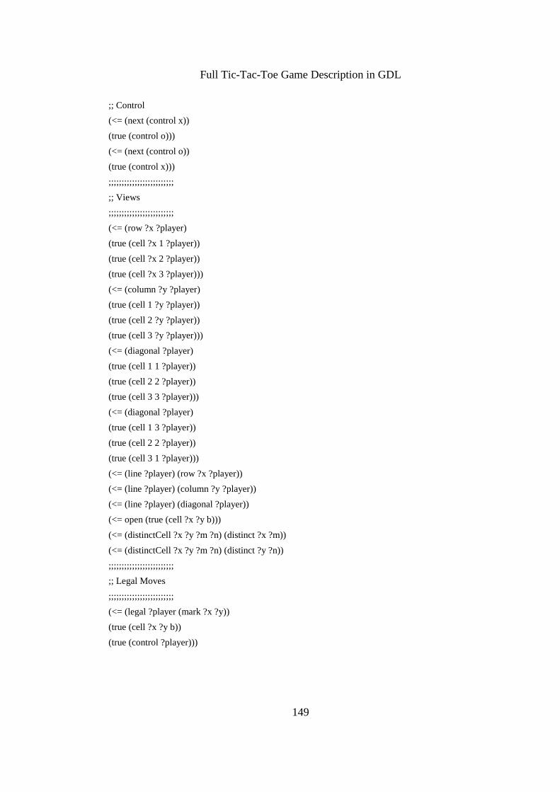
149

Full Tic-Tac-Toe Game Description in GDL

;; Control

(<= (next (control x))

(true (control o)))

(<= (next (control o))

(true (control x)))

;;;;;;;;;;;;;;;;;;;;;;;;;

;; Views

;;;;;;;;;;;;;;;;;;;;;;;;;

(<= (row ?x ?player)

(true (cell ?x 1 ?player))

(true (cell ?x 2 ?player))

(true (cell ?x 3 ?player)))

(<= (column ?y ?player)

(true (cell 1 ?y ?player))

(true (cell 2 ?y ?player))

(true (cell 3 ?y ?player)))

(<= (diagonal ?player)

(true (cell 1 1 ?player))

(true (cell 2 2 ?player))

(true (cell 3 3 ?player)))

(<= (diagonal ?player)

(true (cell 1 3 ?player))

(true (cell 2 2 ?player))

(true (cell 3 1 ?player)))

(<= (line ?player) (row ?x ?player))

(<= (line ?player) (column ?y ?player))

(<= (line ?player) (diagonal ?player))

(<= open (true (cell ?x ?y b)))

(<= (distinctCell ?x ?y ?m ?n) (distinct ?x ?m))

(<= (distinctCell ?x ?y ?m ?n) (distinct ?y ?n))

;;;;;;;;;;;;;;;;;;;;;;;;;

;; Legal Moves

;;;;;;;;;;;;;;;;;;;;;;;;;

(<= (legal ?player (mark ?x ?y))

(true (cell ?x ?y b))

(true (control ?player)))

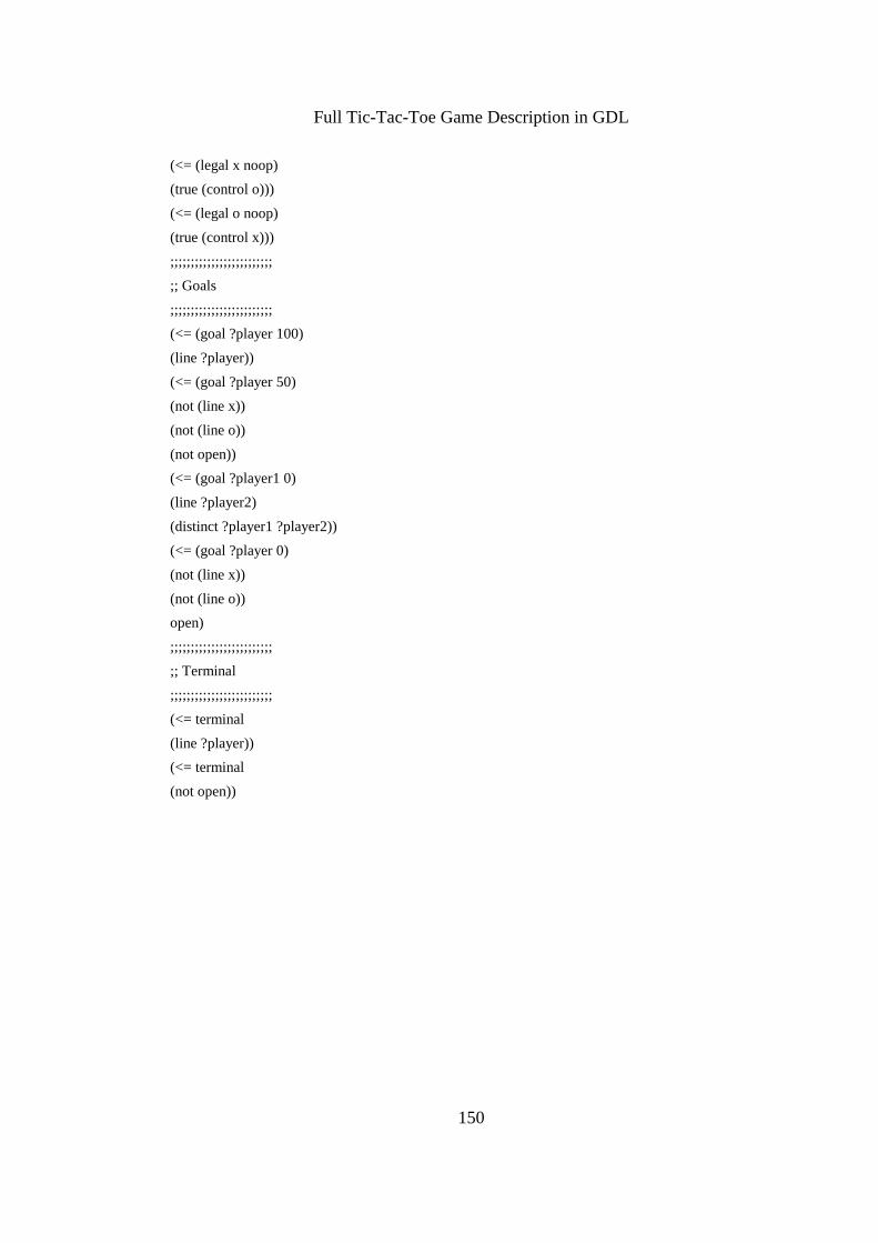
150

Full Tic-Tac-Toe Game Description in GDL

(<= (legal x noop)

(true (control o)))

(<= (legal o noop)

(true (control x)))

;;;;;;;;;;;;;;;;;;;;;;;;;

;; Goals

;;;;;;;;;;;;;;;;;;;;;;;;;

(<= (goal ?player 100)

(line ?player))

(<= (goal ?player 50)

(not (line x))

(not (line o))

(not open))

(<= (goal ?player1 0)

(line ?player2)

(distinct ?player1 ?player2))

(<= (goal ?player 0)

(not (line x))

(not (line o))

open)

;;;;;;;;;;;;;;;;;;;;;;;;;

;; Terminal

;;;;;;;;;;;;;;;;;;;;;;;;;

(<= terminal

(line ?player))

(<= terminal

(not open))

151

APPENDIX C

Full Othello Game Description in GDL

;;;;;;;;;;;;;;;;;;;;;;;;;

;; Roles

;;;;;;;;;;;;;;;;;;;;;;;;;

(role white)

(role black)

;;;;;;;;;;;;;;;;;;;;;;;;;

;; Initial State

;;;;;;;;;;;;;;;;;;;;;;;;;

(init (cell 1 1 green))

(init (cell 1 2 green))

(init (cell 1 3 green))

(init (cell 1 4 green))

(init (cell 1 5 green))

(init (cell 1 6 green))

(init (cell 1 7 green))

(init (cell 1 8 green))

(init (cell 2 1 green))

(init (cell 2 2 green))

(init (cell 2 3 green))

(init (cell 2 4 green))

(init (cell 2 5 green))

(init (cell 2 6 green))

(init (cell 2 7 green))

(init (cell 2 8 green))

(init (cell 3 1 green))

(init (cell 3 2 green))

(init (cell 3 3 green))

(init (cell 3 4 green))

(init (cell 3 5 green))

(init (cell 3 6 green))

(init (cell 3 7 green))

(init (cell 3 8 green))

(init (cell 4 1 green))

(init (cell 4 2 green))

(init (cell 4 3 green))

152

Full Othello Game Description in GDL

(init (cell 4 4 white))

(init (cell 4 5 black))

(init (cell 4 6 green))

(init (cell 4 7 green))

(init (cell 4 8 green))

(init (cell 5 1 green))

(init (cell 5 2 green))

(init (cell 5 3 green))

(init (cell 5 4 black))

(init (cell 5 5 white))

(init (cell 5 6 green))

(init (cell 5 7 green))

(init (cell 5 8 green))

(init (cell 6 1 green))

(init (cell 6 2 green))

(init (cell 6 3 green))

(init (cell 6 4 green))

(init (cell 6 5 green))

(init (cell 6 6 green))

(init (cell 6 7 green))

(init (cell 6 8 green))

(init (cell 7 1 green))

(init (cell 7 2 green))

(init (cell 7 3 green))

(init (cell 7 4 green))

(init (cell 7 5 green))

(init (cell 7 6 green))

(init (cell 7 7 green))

(init (cell 7 8 green))

(init (cell 8 1 green))

(init (cell 8 2 green))

(init (cell 8 3 green))

(init (cell 8 4 green))

(init (cell 8 5 green))

(init (cell 8 6 green))

(init (cell 8 7 green))

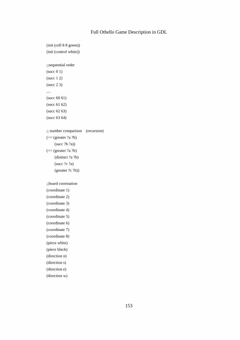
153

Full Othello Game Description in GDL

(init (cell 8 8 green))

(init (control white))

;;sequential order

(succ 0 1)

(succ 1 2)

(succ 2 3)

....

(succ 60 61)

(succ 61 62)

(succ 62 63)

(succ 63 64)

;; number comparison (recursion)

(<= (greater ?a ?b)

(succ ?b ?a))

(<= (greater ?a ?b)

(distinct ?a ?b)

(succ ?c ?a)

(greater ?c ?b))

;;board coorination

(coordinate 1)

(coordinate 2)

(coordinate 3)

(coordinate 4)

(coordinate 5)

(coordinate 6)

(coordinate 7)

(coordinate 8)

(piece white)

(piece black)

(direction n)

(direction s)

(direction e)

(direction w)

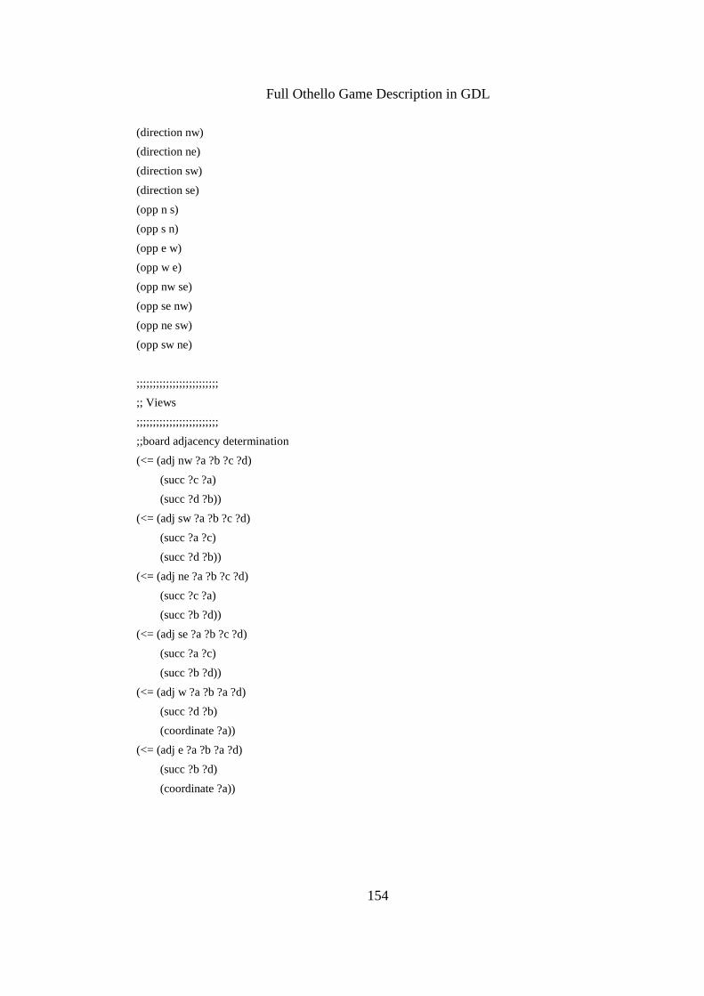
154

Full Othello Game Description in GDL

(direction nw)

(direction ne)

(direction sw)

(direction se)

(opp n s)

(opp s n)

(opp e w)

(opp w e)

(opp nw se)

(opp se nw)

(opp ne sw)

(opp sw ne)

;;;;;;;;;;;;;;;;;;;;;;;;;

;; Views

;;;;;;;;;;;;;;;;;;;;;;;;;

;;board adjacency determination

(<= (adj nw ?a ?b ?c ?d)

(succ ?c ?a)

(succ ?d ?b))

(<= (adj sw ?a ?b ?c ?d)

(succ ?a ?c)

(succ ?d ?b))

(<= (adj ne ?a ?b ?c ?d)

(succ ?c ?a)

(succ ?b ?d))

(<= (adj se ?a ?b ?c ?d)

(succ ?a ?c)

(succ ?b ?d))

(<= (adj w ?a ?b ?a ?d)

(succ ?d ?b)

(coordinate ?a))

(<= (adj e ?a ?b ?a ?d)

(succ ?b ?d)

(coordinate ?a))

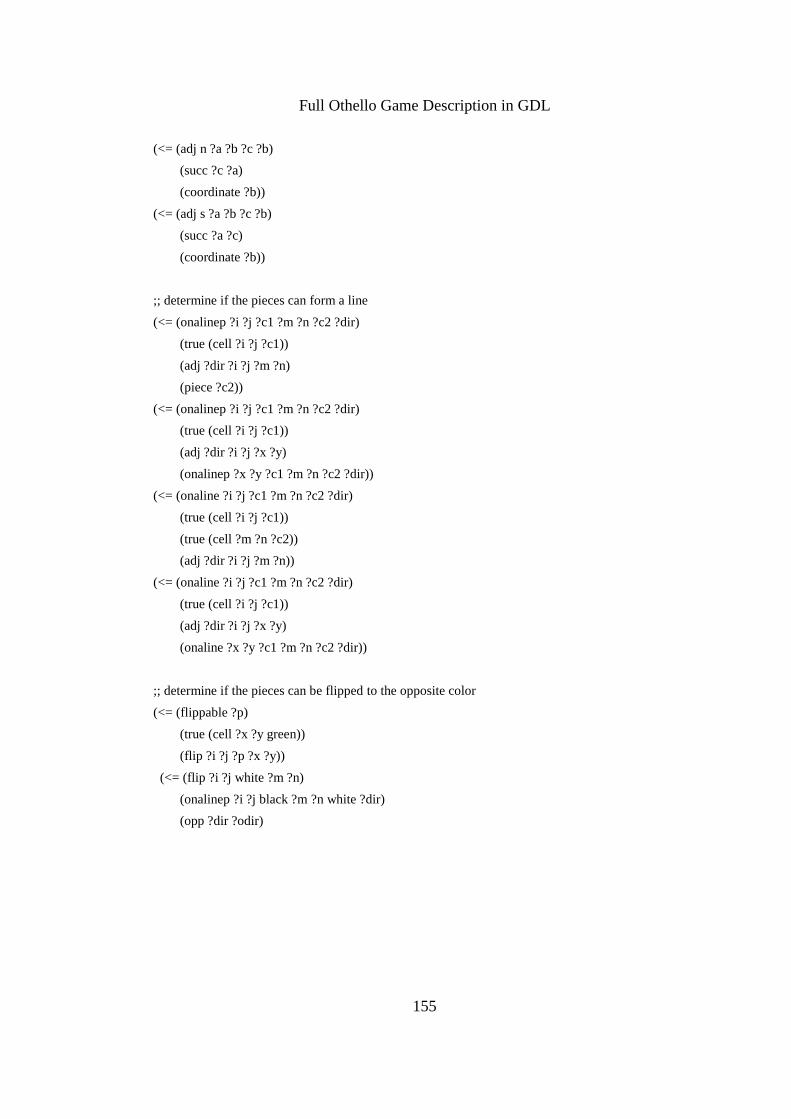
155

Full Othello Game Description in GDL

(<= (adj n ?a ?b ?c ?b)

(succ ?c ?a)

(coordinate ?b))

(<= (adj s ?a ?b ?c ?b)

(succ ?a ?c)

(coordinate ?b))

;; determine if the pieces can form a line

(<= (onalinep ?i ?j ?c1 ?m ?n ?c2 ?dir)

(true (cell ?i ?j ?c1))

(adj ?dir ?i ?j ?m ?n)

(piece ?c2))

(<= (onalinep ?i ?j ?c1 ?m ?n ?c2 ?dir)

(true (cell ?i ?j ?c1))

(adj ?dir ?i ?j ?x ?y)

(onalinep ?x ?y ?c1 ?m ?n ?c2 ?dir))

(<= (onaline ?i ?j ?c1 ?m ?n ?c2 ?dir)

(true (cell ?i ?j ?c1))

(true (cell ?m ?n ?c2))

(adj ?dir ?i ?j ?m ?n))

(<= (onaline ?i ?j ?c1 ?m ?n ?c2 ?dir)

(true (cell ?i ?j ?c1))

(adj ?dir ?i ?j ?x ?y)

(onaline ?x ?y ?c1 ?m ?n ?c2 ?dir))

;; determine if the pieces can be flipped to the opposite color

(<= (flippable ?p)

(true (cell ?x ?y green))

(flip ?i ?j ?p ?x ?y))

(<= (flip ?i ?j white ?m ?n)

(onalinep ?i ?j black ?m ?n white ?dir)

(opp ?dir ?odir)

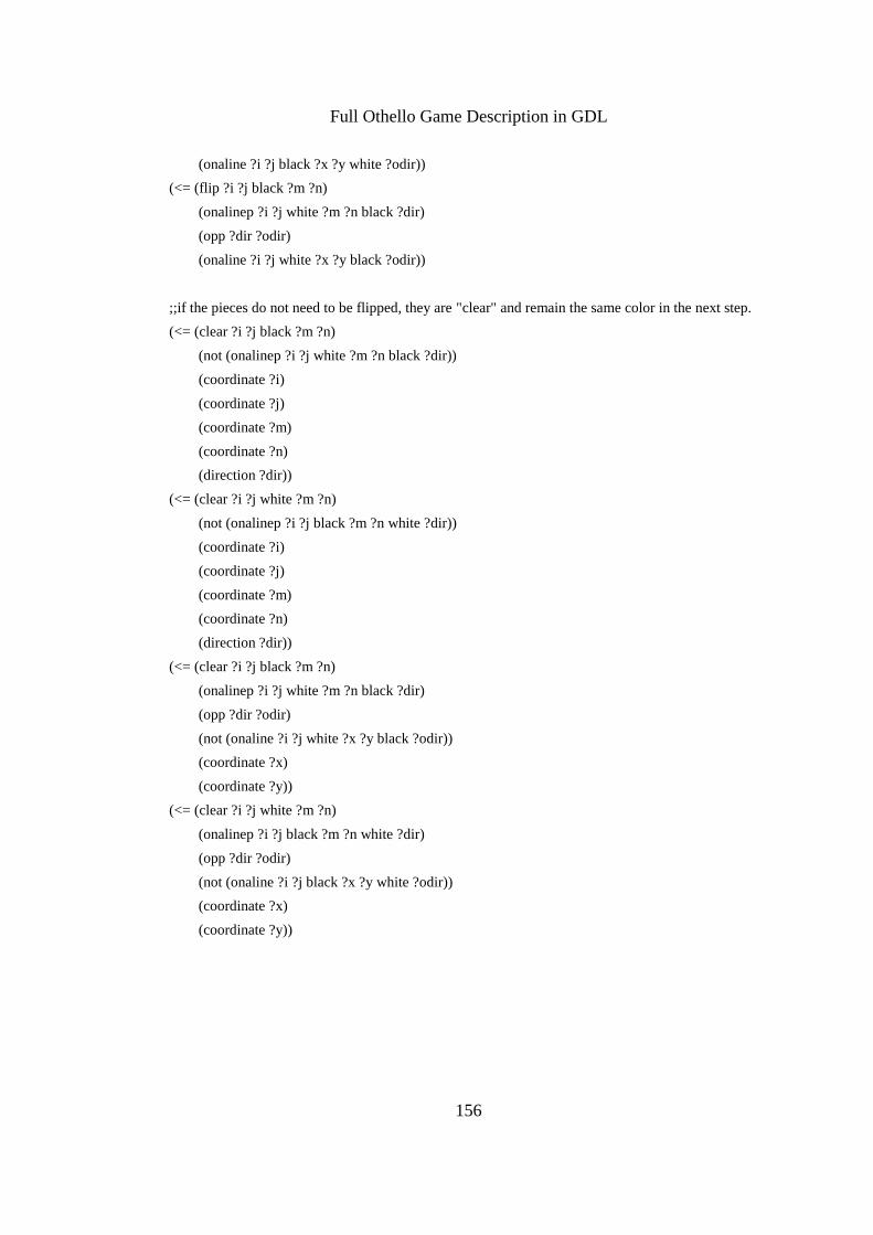
156

Full Othello Game Description in GDL

(onaline ?i ?j black ?x ?y white ?odir))

(<= (flip ?i ?j black ?m ?n)

(onalinep ?i ?j white ?m ?n black ?dir)

(opp ?dir ?odir)

(onaline ?i ?j white ?x ?y black ?odir))

;;if the pieces do not need to be flipped, they are "clear" and remain the same color in the next step.

(<= (clear ?i ?j black ?m ?n)

(not (onalinep ?i ?j white ?m ?n black ?dir))

(coordinate ?i)

(coordinate ?j)

(coordinate ?m)

(coordinate ?n)

(direction ?dir))

(<= (clear ?i ?j white ?m ?n)

(not (onalinep ?i ?j black ?m ?n white ?dir))

(coordinate ?i)

(coordinate ?j)

(coordinate ?m)

(coordinate ?n)

(direction ?dir))

(<= (clear ?i ?j black ?m ?n)

(onalinep ?i ?j white ?m ?n black ?dir)

(opp ?dir ?odir)

(not (onaline ?i ?j white ?x ?y black ?odir))

(coordinate ?x)

(coordinate ?y))

(<= (clear ?i ?j white ?m ?n)

(onalinep ?i ?j black ?m ?n white ?dir)

(opp ?dir ?odir)

(not (onaline ?i ?j black ?x ?y white ?odir))

(coordinate ?x)

(coordinate ?y))

157

Full Othello Game Description in GDL

;; counting the pieces on the board

(<= (count ?row ?column ?whitenum ?blacknum)

(distinct ?column 8)

(true (cell ?row ?column white))

(succ ?column ?nc)

(count ?row ?nc ?rest ?blacknum)

(succ ?rest ?whitenum))

(<= (count ?row ?column ?whitenum ?blacknum)

(distinct ?column 8)

(true (cell ?row ?column black))

(succ ?column ?nc)

(count ?row ?nc ?whitenum ?rest)

(succ ?rest ?blacknum))

(<= (count ?row ?column ?whitenum ?blacknum)

(distinct ?column 8)

(true (cell ?row ?column green))

(succ ?column ?nc)

(count ?row ?nc ?whitenum ?blacknum))

(<= (count ?row 8 ?whitenum ?blacknum)

(distinct ?row 8)

(true (cell ?row 8 white))

(succ ?row ?nr)

(count ?nr 1 ?rest ?blacknum)

(succ ?rest ?whitenum))

(<= (count ?row 8 ?whitenum ?blacknum)

(distinct ?row 8)

(true (cell ?row 8 black))

(succ ?row ?nr)

(count ?nr 1 ?whitenum ?rest)

(succ ?rest ?blacknum))

(<= (count ?row 8 ?whitenum ?blacknum)

(distinct ?row 8)

(true (cell ?row 8 green))

(succ ?row ?nr)

(count ?nr 1 ?whitenum ?blacknum))

158

Full Othello Game Description in GDL

(<= (count 8 8 1 0)

(true (cell 8 8 white)))

(<= (count 8 8 0 1)

(true (cell 8 8 black)))

(<= (count 8 8 0 0)

(true (cell 8 8 green)))

;;;;;;;;;;;;;;;;;;;;;;;;;

;; Dynamic Components

;;;;;;;;;;;;;;;;;;;;;;;;;

(<= (next (cell ?m ?n white))

(does white (place ?m ?n))

(true (cell ?m ?n green)))

(<= (next (cell ?m ?n black))

(does black (place ?m ?n))

(true (cell ?m ?n green)))

(<= (next (cell ?m ?n white))

(true (cell ?m ?n black))

(does white (place ?i ?j))

(flip ?m ?n white ?i ?j))

(<= (next (cell ?m ?n black))

(true (cell ?m ?n white))

(does black (place ?i ?j))

(flip ?m ?n black ?i ?j))

(<= (next (cell ?m ?n white))

(true (cell ?m ?n white))

(does white (place ?x ?y)))

(<= (next (cell ?m ?n black))

(true (cell ?m ?n black))

(does black (place ?x ?y)))

(<= (next (cell ?m ?n black))

(true (cell ?m ?n black))

(does white (place ?i ?j))

(clear ?m ?n white ?i ?j))

159

Full Othello Game Description in GDL

(<= (next (cell ?m ?n white))

(true (cell ?m ?n white))

(does black (place ?i ?j))

(clear ?m ?n black ?i ?j))

(<= (next (cell ?m ?n green))

(does ?w (place ?j ?k))

(true (cell ?m ?n green))

(or (distinct ?m ?j) (distinct ?n ?k)))

(<= (next (cell ?m ?n ?color))

(true (cell ?m ?n ?color))

(true (control ?p))

(does ?p noop))

;;;;;;;;;;;;;;;;;;;;;;;;;

;; Controls

;;;;;;;;;;;;;;;;;;;;;;;;;

(<= (next (control white))

(true (control black)))

(<= (next (control black))

(true (control white)))

;;;;;;;;;;;;;;;;;;;;;;;;;

;; Legal Moves

;;;;;;;;;;;;;;;;;;;;;;;;;

(<= (legal white (place ?m ?n))

(true (control white))

(true (cell ?m ?n green))

(flip ?i ?j white ?m ?n))

(<= (legal black (place ?m ?n))

(true (control black))

(true (cell ?m ?n green))

(flip ?i ?j black ?m ?n))

(<= (legal white noop)

(true (cell ?x ?y green))

(true (control black)))

(<= (legal black noop)

(true (cell ?x ?y green))

(true (control white)))

160

Full Othello Game Description in GDL

(<= (legal ?p noop)

(true (control ?p))

(not (flippable ?p)))

;;;;;;;;;;;;;;;;;;;;;;;;;

;;Goals

;;;;;;;;;;;;;;;;;;;;;;;;;

(<= (goal white 100)

(count 1 1 ?w ?b)

(greater ?w ?b))

(<= (goal black 100)

(count 1 1 ?w ?b)

(greater ?b ?w))

(<= (goal ?role 50)

(count 1 1 ?x ?x)

(role ?role))

(<= (goal black 0)

(count 1 1 ?w ?b)

(greater ?w ?b))

(<= (goal white 0)

(count 1 1 ?w ?b)

(greater ?b ?w))

(<= open

(true (cell ?m ?n green)))

;;;;;;;;;;;;;;;;;;;;;;;;;

;; Terminal

;;;;;;;;;;;;;;;;;;;;;;;;;

(<= terminal

(not open))

(<= terminal

(not (flippable white))

(not (flippable black)))

161

APPENDIX D

A Complete Tic-Tac-Toe Match with HTTP Communications

POST / HTTP/1.0

Accept: text/delim

Sender: GAMEMASTER

Receiver: GAMEPLAYER

Content-type: text/acl

Content-length: 1554

(START MATCH.3316980891 X

(ROLE X) (ROLE O) (INIT (CELL 1 1 B)) (INIT (CELL 1 2 B)) (INIT (CELL 1 3 B))

(INIT (CELL 2 1 B)) (INIT (CELL 2 2 B)) (INIT (CELL 2 3 B)) (INIT (CELL 3 1 B))

(INIT (CELL 3 2 B)) (INIT (CELL 3 3 B)) (INIT (CONTROL X))

(<= (NEXT (CELL ?X ?Y ?PLAYER)) (DOES ?PLAYER (MARK ?X ?Y)))

(<= (NEXT (CELL ?X ?Y ?MARK)) (TRUE (CELL ?X ?Y ?MARK)) (DOES ?PLAYER

(MARK ?M ?N))

(DISTINCTCELL ?X ?Y ?M ?N)) (<= (NEXT (CONTROL X)) (TRUE (CONTROL O)))

(<= (NEXT (CONTROL O)) (TRUE (CONTROL X))) (<= (ROW ?X ?PLAYER) (TRUE (CELL ?X

1 ?PLAYER))

(TRUE (CELL ?X 2 ?PLAYER)) (TRUE (CELL ?X 3 ?PLAYER))) (<= (COLUMN ?Y ?PLAYER)

(TRUE (CELL 1 ?Y ?PLAYER)) (TRUE (CELL 2 ?Y ?PLAYER)) (TRUE (CELL

3 ?Y ?PLAYER)))

(<= (DIAGONAL ?PLAYER) (TRUE (CELL 1 1 ?PLAYER)) (TRUE (CELL 2 2 ?PLAYER))

(TRUE (CELL 3 3 ?PLAYER))) (<= (DIAGONAL ?PLAYER) (TRUE (CELL 1 3 ?PLAYER))

(TRUE (CELL 2 2 ?PLAYER)) (TRUE (CELL 3 1 ?PLAYER))) (<= (LINE ?PLAYER)

(ROW ?X ?PLAYER))

(<= (LINE ?PLAYER) (COLUMN ?Y ?PLAYER)) (<= (LINE ?PLAYER)

(DIAGONAL ?PLAYER))

(<= OPEN (TRUE (CELL ?X ?Y B))) (<= (DISTINCTCELL ?X ?Y ?M ?N) (DISTINCT ?X ?M))

(<= (DISTINCTCELL ?X ?Y ?M ?N) (DISTINCT ?Y ?N)) (<= (LEGAL ?PLAYER

(MARK ?X ?Y))

(TRUE (CELL ?X ?Y B)) (TRUE (CONTROL ?PLAYER))) (<= (LEGAL ?PLAYER NOOP)

(NOT (TRUE (CONTROL ?PLAYER)))) (<= (GOAL ?PLAYER 100) (LINE ?PLAYER))

(<= (GOAL ?PLAYER 50) (NOT (LINE X)) (NOT (LINE O)) (NOT OPEN)) (<=

(GOAL ?PLAYER1 0)

(LINE ?PLAYER2) (DISTINCT ?PLAYER1 ?PLAYER2)) (<= (GOAL ?PLAYER 0) (NOT (LINE

X))

162

A Complete Tic-Tac-Toe Match with HTTP Communications

(NOT (LINE O)) OPEN) (<= TERMINAL (LINE ?PLAYER)) (<= TERMINAL (NOT OPEN))

30 30)

HTTP/1.0 200 OK

Content-type: text/acl

Content-length: 5

READY

POST / HTTP/1.0

Accept: text/delim

Sender: GAMEMASTER

Receiver: GAMEPLAYER

Content-type: text/acl

Content-length: 27

(PLAY MATCH.3316980891 NIL)

HTTP/1.0 200 OK

Content-type: text/acl

Content-length: 10

(MARK 3 3)

POST / HTTP/1.0

Accept: text/delim

Sender: GAMEMASTER

Receiver: GAMEPLAYER

Content-type: text/acl

Content-length: 40

(PLAY MATCH.3316980891 ((MARK 3 3) NOOP))

HTTP/1.0 200 OK

Content-type: text/acl

Content-length: 4

NOOP

POST / HTTP/1.0

Accept: text/delim

Sender: GAMEMASTER

Receiver: GAMEPLAYER

Content-type: text/acl

Content-length: 40

163

A Complete Tic-Tac-Toe Match with HTTP Communications

(PLAY MATCH.3316980891 (NOOP (MARK 1 3)))

HTTP/1.0 200 OK

Content-type: text/acl

Content-length: 10

(MARK 2 2)

POST / HTTP/1.0

Accept: text/delim

Sender: GAMEMASTER

Receiver: GAMEPLAYER

Content-type: text/acl

Content-length: 40

(PLAY MATCH.3316980891 ((MARK 2 2) NOOP))

HTTP/1.0 200 OK

Content-type: text/acl

Content-length: 4

NOOP

POST / HTTP/1.0

Accept: text/delim

Sender: GAMEMASTER

Receiver: GAMEPLAYER

Content-type: text/acl

Content-length: 40

(PLAY MATCH.3316980891 (NOOP (MARK 1 2)))

HTTP/1.0 200 OK

Content-type: text/acl

Content-length: 10

(MARK 1 1)

POST / HTTP/1.0

Accept: text/delim

Sender: GAMEMASTER

Receiver: GAMEPLAYER

Content-type: text/acl

Content-length: 40

164

A Complete Tic-Tac-Toe Match with HTTP Communications

(STOP MATCH.3316980891 ((MARK 1 1) NOOP))

HTTP/1.0 200 OK

Content-type: text/acl

Content-length: 4

DONE

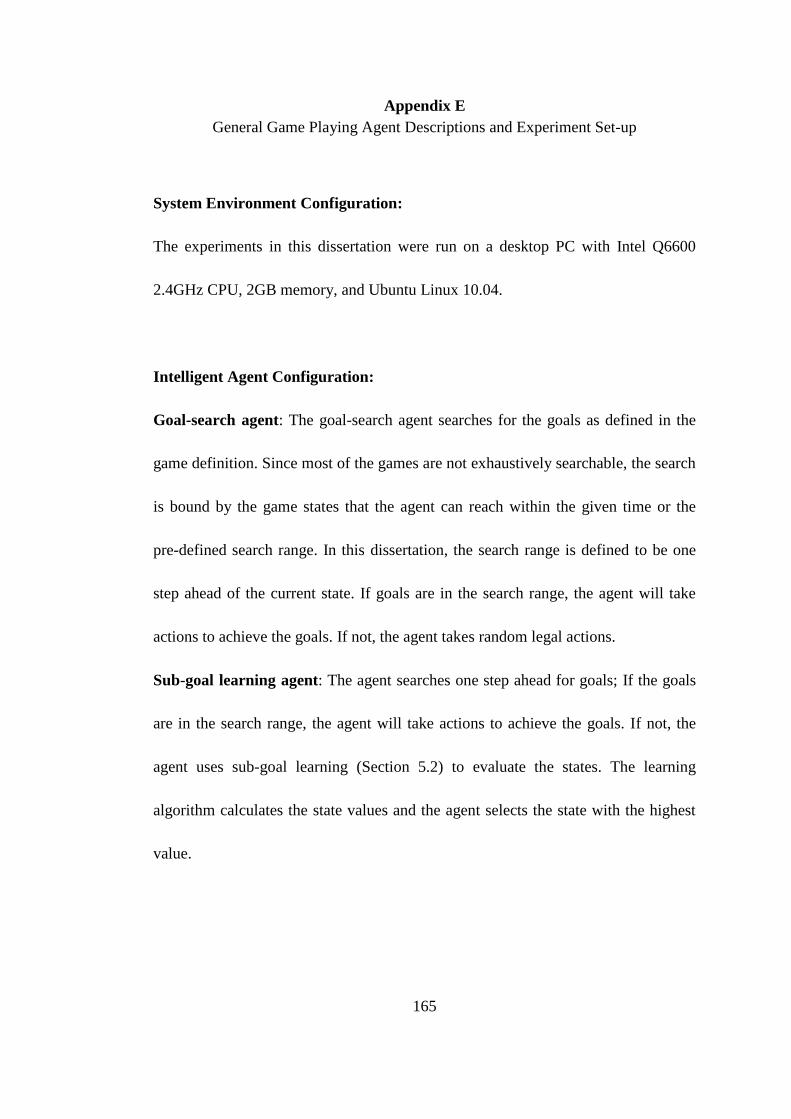
165

Appendix E

General Game Playing Agent Descriptions and Experiment Set-up

System Environment Configuration:

The experiments in this dissertation were run on a desktop PC with Intel Q6600

2.4GHz CPU, 2GB memory, and Ubuntu Linux 10.04.

Intelligent Agent Configuration:

Goal-search agent: The goal-search agent searches for the goals as defined in the

game definition. Since most of the games are not exhaustively searchable, the search

is bound by the game states that the agent can reach within the given time or the

pre-defined search range. In this dissertation, the search range is defined to be one

step ahead of the current state. If goals are in the search range, the agent will take

actions to achieve the goals. If not, the agent takes random legal actions.

Sub-goal learning agent: The agent searches one step ahead for goals; If the goals

are in the search range, the agent will take actions to achieve the goals. If not, the

agent uses sub-goal learning (Section 5.2) to evaluate the states. The learning

algorithm calculates the state values and the agent selects the state with the highest

value.

166

General Game Playing Agent Descriptions and Experiment Set-up

Decision tree learning agent: The agent searches one step ahead for goals. If the

goals are in the search range, the agent will take actions to achieve the goals. If not,

the agent uses decision tree learning (Section 6.2) to evaluate the states. The learning

algorithm calculates the state values and the agent selects the state with the highest

value.

Contextual Decision Tree Learning agent: The agent searches one-step ahead for

goals. If the goals are in the search range, the agent will take actions to achieve the

goals. If not, the agent uses contextual decision tree learning (Section 6.3) to evaluate

the states. The learning algorithm calculates the state values and the agent selects the

state with the highest value.

Random Players: Random players are used to build a self-play simulation database

(Section 5.1). They are also used when evaluating the performance of the intelligence

player. When there is more than one player in the game, the first player is set to be the

intelligent player that uses different learning algorithms and the remaining players are

set to be dummy players. It uses the same reasoning engine to retrieve legal actions.

167

General Game Playing Agent Descriptions and Experiment Set-up

The agent randomly selects one action in the legal action list. The purpose of using the

random players is to create different paths of the same game and collect statistical data

for analysis.