GMTSAR:An InSAR Processing System

Based on Generic Mapping Tools

(Second Edition)

David Sandwell∗ Rob Mellors† Xiaopeng Tong∗‡

Xiaohua Xu∗ Matt Wei§ Paul Wessel¶

May 1, 2011; Revised: June 1, 2016

∗Scripps Institution of Oceanography, University of California, San Diego, La Jolla, CA†Lawrence Livermore National Laboratory, Livermore, CA‡Department of Earth and Space Sciences, University of Washington, Seattle, WA§Graduate School of Oceanography, University of Rhode Island, Narragansett, RI¶Department of Geology and Geophysics, University of Hawaii at Manoa, HI

1

Contents1 Introduction 5

1.1 Objectives and limitations of GMTSAR . . . . . . . . . . . . . . . . 51.2 Algorithms: SAR, InSAR, and the need for precise orbits . . . . . . . 6

1.2.1 Proper focus . . . . . . . . . . . . . . . . . . . . . . . . . . 71.2.2 Transformation from geographic to radar coordinates . . . . . 81.2.3 Image alignment . . . . . . . . . . . . . . . . . . . . . . . . 91.2.4 Flattening interferogram - no trend removal . . . . . . . . . . 10

2 Software 112.1 Standard Products . . . . . . . . . . . . . . . . . . . . . . . . . . . . 112.2 Software Design . . . . . . . . . . . . . . . . . . . . . . . . . . . . . 12

3 Processing Examples 143.1 Two-pass processing . . . . . . . . . . . . . . . . . . . . . . . . . . 153.2 Stacking for time series . . . . . . . . . . . . . . . . . . . . . . . . . 183.3 ScanSAR Interferometry . . . . . . . . . . . . . . . . . . . . . . . . 26

4 Problems 32

A Principles of Synthetic Aperture Radar 33A.1 Introduction . . . . . . . . . . . . . . . . . . . . . . . . . . . . . . . 33A.2 Fraunhoffer diffraction . . . . . . . . . . . . . . . . . . . . . . . . . 34A.3 2-D Aperture . . . . . . . . . . . . . . . . . . . . . . . . . . . . . . 37A.4 Range resolution (end view) . . . . . . . . . . . . . . . . . . . . . . 38A.5 Azimuth resolution (top view) . . . . . . . . . . . . . . . . . . . . . 39A.6 Range and Azimuth Resolution of ERS SAR . . . . . . . . . . . . . . 40A.7 Pulse repetition frequency . . . . . . . . . . . . . . . . . . . . . . . 40A.8 Other constraints on the PRF . . . . . . . . . . . . . . . . . . . . . . 40A.9 Problems . . . . . . . . . . . . . . . . . . . . . . . . . . . . . . . . 42

B SAR Image Formation 44B.1 Overview of the range-doppler algorithm . . . . . . . . . . . . . . . 44B.2 Processing on board the satellite . . . . . . . . . . . . . . . . . . . . 44B.3 Digital SAR processing . . . . . . . . . . . . . . . . . . . . . . . . . 45B.4 Range compression . . . . . . . . . . . . . . . . . . . . . . . . . . . 49B.5 Azimuth compression . . . . . . . . . . . . . . . . . . . . . . . . . . 51B.6 Example with ALOS L-band orbit . . . . . . . . . . . . . . . . . . . 58B.7 Problems . . . . . . . . . . . . . . . . . . . . . . . . . . . . . . . . 61

C InSAR 62C.1 Forming an interferogram . . . . . . . . . . . . . . . . . . . . . . . . 62C.2 Contributions to Phase . . . . . . . . . . . . . . . . . . . . . . . . . 63C.3 Phase due to earth curvature . . . . . . . . . . . . . . . . . . . . . . 64C.4 Look angle and incidence angle for a spherical earth . . . . . . . . . . 65C.5 Critical baseline . . . . . . . . . . . . . . . . . . . . . . . . . . . . . 67

2

C.6 Persistent point scatterer and critical baseline . . . . . . . . . . . . . 68C.7 Phase due to topography . . . . . . . . . . . . . . . . . . . . . . . . 69C.8 Altitude of ambiguity . . . . . . . . . . . . . . . . . . . . . . . . . . 70C.9 Phase due to earth curvature and topography – exact formula . . . . . 70C.10 Problems . . . . . . . . . . . . . . . . . . . . . . . . . . . . . . . . 74

D ScanSAR Processing and Interferometry 75D.1 Problems . . . . . . . . . . . . . . . . . . . . . . . . . . . . . . . . 80

E Sentinel TOPS-mode processing and interferometry 81E.1 Introduction . . . . . . . . . . . . . . . . . . . . . . . . . . . . . . . 81E.2 Traditional Image Alignment Fails with TOPS-Mode Data . . . . . . 83E.3 Geometric Image Registration . . . . . . . . . . . . . . . . . . . . . 84E.4 Enhanced Spectral Diversity . . . . . . . . . . . . . . . . . . . . . . 86E.5 Elevation Antenna Pattern (EAP) Correction (IPF version change) . . 87E.6 Examples of TOPS Interferogram processing . . . . . . . . . . . . . 87E.7 Processing setup and commands: . . . . . . . . . . . . . . . . . . . . 97E.8 Problems . . . . . . . . . . . . . . . . . . . . . . . . . . . . . . . . 99

F Geolocation accuracy for Pinon corner reflectors 100

G Installation of GMTSAR 107

3

Preface to Second EditionThis technical report provides an update to the original GMTSAR report published in2011. The significant changes to the software and documentation include:

• preprocessors for new data types including TerraSAR-X, COSMO-SkyMed, Radar-sat-2, ALOS-2, and Sentinel-1;

• the addition of a coherence-based SBAS time series program;

• full integration of GMTSAR with GMT5;

• geometric image alignment based only on orbits and topography; and

• full support for Sentinel-1 TOPS-mode data.

The addition of the TOPS-mode processing involved a refinement of the algorithm fortransforming between geographic and radar coordinates that is now accurate to a fewcentimeters. Pure geometric image alignment of all slaves to a single master enablesa whole new approach to data preparation for InSAR time series. GMTSAR is stillfocussed on the basic aspects of InSAR processing to prepare large stacks of imagesfor more advanced time series method such as persistent scatterer analysis. We haveavoided constructing tools that can hide fundamental limitations in the data or software(e.g., baseline re-estimation). Our objective is to keep the core software small andonly dependent on Generic Mapping Tools. GMTSAR also uses a published phaseunrapping code called Snaphu (Chen and Zebker 2000). The user can use GMT orother packages for post processing (e.g., combining InSAR with GPS point data). Thissoftware is completely open under a GNU General Public License so users should feelfree to modify and redistribute codes. The best way to learn to use GMTSAR is toinstall it and run the test examples. In addition, for the past several years we haveoffered a short course sponsored by UNAVCO. The instructional material is posted atthe UNAVCO short course site.

4

1 IntroductionGMTSAR is an open source (GNU General Public License) InSAR processing systemdesigned for users familiar with Generic Mapping Tools (GMT). The code is writtenin C and will compile on any computer where GMT and NETCDF are installed. Thesystem has three main components: 1) a preprocessor for each satellite data type toconvert the native format and orbital information into a generic format; 2) an InSARprocessor to focus and align stacks of images, map topography into phase, and form thecomplex interferogram; 3) a postprocessor, mostly based on GMT, to filter the inter-ferogram and construct interferometric products of phase, coherence, phase gradient,and line-of-sight displacement in both radar and geographic coordinates. GMT is usedto display all the products as postscript files and kml-images for Google Earth. A setof C-shell scripts has been developed for standard 2-pass processing as well as imagealignment for stacking and time series. Users are welcome to contribute to this effort.

GMTSAR differs from other InSAR systems such as ROI PAC, Gamma, and DORISbecause it relies on sub-meter orbital accuracy to greatly simplify the SAR and InSARprocessing algorithms. Moreover large batches of SAR images can be automaticallyprocessed with no human intervention. The down side of this approach is that SARsatellites having less accurate orbits (> 10 m, e.g., RADARSAT-1 and JERS-1) cannotbe easily processed using GMTSAR. Reliance on precise orbits also greatly simplifiesthe code so only 5 essential programs (llt2rat, esarp, xcorr, phasediff, conv) are neededbeyond the GMT package. Moreover, geometric and phase accuracy ensures that mo-saics of many frames along a long swath or combinations of ScanSAR subswaths willabut seamlessly in geographic coordinates. This document contains three main sectionsand 7 appendices. Section 1 is an introduction to GMTSAR and the geometric modelused to create SAR and InSAR products without using ground control or applying or-bital adjustments. Section 2 is a description of the overall software design as well asthe standard output products. Section 3 provides recipes for the most common types ofInSAR processing including 2-pass InSAR, stacking/time series, and ScanSAR inter-ferometry. Appendix A is an overview of principles of SAR processing. Appendix Bis a detailed description of the range-Doppler SAR processor and the parameter file.Appendix C provides the theory for InSAR processing on a spherical Earth with no ap-proximations. Appendix D describes the algorithm that we use for ALOS-1 ScanSARinterferometry. Appendix E describes the geometric image alignment algorithms de-veloped for the TOPS-mode data from Sentinel-1. Appendix F provides data on thegeolocation accuracy of SAR imagery. Appendix G provides instructions for installa-tion and testing the GMTSAR package.

1.1 Objectives and limitations of GMTSARCreating synthetic aperture radar (SAR) images and interferograms (InSAR) fromsatellite radar measurements requires specialized front-end computer codes for focus-ing imagery and computing interferometric phase. However, much of the back-endprocessing and display can be accomplished with existing generic codes. We have de-veloped a SAR/InSAR processing system that starts with raw (or SLC) SAR data inradar coordinates, along with precise orbital information, and computes interferomet-

5

ric products in geographic coordinates. Our design goals are to have a modular andportable system based on a minimum set of new software. The system relies on preciseorbital information, as discussed below, and a consistent geometric model to achieveproper focus and image alignment. The SAR processor code was originally derivedfrom the Stanford/JPL FORTRAN and re-written in the C programming language en-suring compilation on many platforms using the standard gcc compiler. The remainderof the front-end code has been developed and refined over the past decade as part ofthe SIOSAR and ALOS preprocess packages.

For the back-end processing we use the Generic Mapping Tools (GMT), which isan open source collection of programs designed for manipulating and displaying ge-ographic data sets (Wessel and Smith 1998; Wessel, Smith, et al. 2013). It is widelyused among the geophysical community, well documented, and continuously updated.GMT includes efficient and robust programs for regridding, filtering, and trend re-moval, which makes it highly useful for some aspects of InSAR processing. GMT usesthe NETCDF file format that allows the exchange of files among computers havingdifferent architectures. The combined front- and back-end processing is done usingthe c-shell scripting language which is available on all UNIX platforms. We encour-age the development of new modules and InSAR processing recipes from the broaderInSAR community. The GMTSAR package also includes the capability for ScanSARprocessing and is flexible enough for performing time series analysis on stacks of in-terferograms.

1.2 Algorithms: SAR, InSAR, and the need for precise orbitsSynthetic aperture radar (SAR) satellites collect swaths of side-looking echoes at a suf-ficiently high range resolution and along-track sampling rate to form high resolutionimagery (Appendix A). The range resolution of the raw radar data is determined bythe pulse length (or 1/bandwidth) and the incidence angle; a typical range resolutionis 20 m. For real aperture radar, the along-track or azimuth resolution of the outgoingmicrowave pulse is diffraction limited to an angle corresponding to the wavelength ofthe radar (e.g. 0.05 m) divided by the length of the aperture (e.g. 10 m). When thisbeam pattern is projected onto the surface of the earth at a range of say 850 km, it illu-minates 4250 m in the along-track dimension so the raw radar data are horribly out offocus in azimuth. Using the synthetic aperture method, the image can be focused on apoint reflector on the ground by coherently summing thousands of consecutive echoesthus creating a synthetic aperture perhaps 4250 m long. Proper focus is achieved bysumming the complex numbers along a constant range. The focused image containsboth amplitude (backscatter) and phase (range) information for each pixel. In GMT-SAR, the SAR processor computer code is called esarp; proper focus relies on havingan accurate orbital trajectory for the satellite (Appendix B). For example the image willbe out of focus if the range between the antenna and reflector has an error greater thanabout 1/4 wavelength (e.g. 0.01 m) over a distance of the synthetic aperture (4250 m).

A complex radar interferogram (InSAR) is created by multiplying the referenceimage by the complex conjugate of the repeat image (Appendix C). For the ideal casewhere the trajectories of the reference and repeat images are exactly coincident, thephase difference between the two images will reflect differences in range between the

6

antenna and a target pixel. This could be due to line-of-sight motion of the targetpixel or a travel time change due to the atmosphere or ionosphere. Normally there isan offset between the trajectories of the reference and repeat orbits. In this case thephase of the complex interferogram has an additional component due to the shape ofthe earth. The corrections for the curvature and topography of the earth are combinedinto one formula in the code phasediff (Appendix C). This topographic phase can beremoved from the interferogram if independent topography information is available(e.g., SRTM (Farr et al. 2004)). An accurate orbit is needed to project the topographymodel from a latitude, longitude, and ellipsoidal height coordinate system into therange and azimuth coordinates of the radar image. An accurate orbit is also neededto correct the phase of the repeat image for the non-zero interferometric baseline sinceorbital error maps directly into interferometric phase. The GMTSAR software will onlyprovide reliable output for interferometric satellites where precise orbital information(<1 m precision) is available. Today this includes (ERS-1, ERS-2, Envisat, ALOS-1,and TerraSAR-X, COSMO-SkyMed, Radarsat-2, ALOS-2, and Sentinel-1). Note thatRadarsat-1 and JERS-1 cannot be easily processed with this software because theirorbits are not accurate enough. The precise orbital information is used in 4 aspectsof the InSAR processing discussed in the following text and is the key to robust andefficient software.

1.2.1 Proper focus

First proper focus of the SAR image involves the coherent summation of range-alignedechoes over the length of the synthetic aperture as shown in Figure 1. Therefore weneed to calculate the range as a function of slow time s. First consider the case of astraight line orbit passing over a fixed point reflector. The range to the reflector wouldvary as a hyperbola with slow time. In the actual case the orbital path is elliptical andthe earth is rotating so the range versus time function is a more complicated function.However, because the synthetic aperture is short (<5 km) compared with the nominalrange from the satellite to the reflector ( 800 km), a 3-parameter parabolic approxima-tion is commonly used to model range versus time (Curlander and McDonough 1991,Appendix B).

R(s) = Ro + R(s − so) +R2

(s − so)2 + · · · (1)

where Ro is the closest approach of the spacecraft to the point reflector and so is thetime of closest approach. These three parameters Ro, R, and R are needed to focus animage (Appendix B). In terms of the SAR processor, these are called the near range Ro,the Doppler centroid fDC and the Doppler frequency rate fR which are related to thecoefficients of this polynomial

fDC =−2Rλ

and fR =−2Rλ

, (2)

where λ is the wavelength of the radar. When a SAR image is focused at zero Doppler,the range rate at position so is by definition zero.

7

s

R(s)

pointreflector

Figure 1: Geometry of SAR antenna flying over a point reflector on the ground. Therange R varies with slow time s as measured by the precise orbit provided in an earth-fixed coordinate system.

1.2.2 Transformation from geographic to radar coordinates

The second use of precise orbital information is to map every point on the surface ofthe earth (lon, lat, topography) into the range and azimuth coordinates of the radar.This mapping provides a lookup table for transforming between geographic and radarcoordinates. The algorithm for creating this mapping is conceptually simple but canbe computationally expensive. The precise orbital information is used to determinethe range from the satellite to a topography grid cell. The time of the minimum rangeis found using a Golden section search algorithm (Press et al. 1992). A second orderpolynomial is fit to this range versus time function about the time of minimum range(equation (1)). If the SAR image is focused at zero Doppler then the range coordinateof the mapping is simply the minimum range and the azimuth coordinate is the time ofthe minimum range. Of course, by definition the range-rate, or Doppler, is zero at thisazimuth position. If the radar image was focused at a Doppler centroid other than zerothen equation (2) can be used to calculate the non-zero range-rate at this Doppler.

R = −λ fDC

2(3)

Next by taking the derivative of the parabolic approximation one can determine thealong-track time shift that will be produced by focusing at a non-zero Doppler. This is

8

given by

∆s = −λ fDC

2R(4)

The corresponding range correction is given by

∆R =R2

∆s2. (5)

This mapping from earth to radar coordinates described in equations 1-5 is perhaps theonly really new aspect of GMTSAR and it allows a large simplification of the front-endprocessing code with respect to a more tolerant package such as ROI PAC.

These two corrections are needed in the transformation from geographic to radarcoordinates when the image is focussed at a Doppler other than zero. The accuracy ofthis approach where no ground control points are used has been determined using cor-ner reflectors at Pinon Flat Observatory (Table 1). We have verified the accuracy of ourapproach using raw and SLC SAR imagery from a variety of satellite radars and modes(Table 2 and Appendix F). The L-band results show a systematic range bias perhaps re-lated to the ionosphere and troposphere delays (i.e., the dry troposphere should be -5.8m). The rms variation is typically 6 m in range and 4 m in azimuth. For the ScanSARdata the azimuth positions are 5 times less accurate due to the lower sampling densityin each of the 5 subswaths. Since the highest resolution global topography data for theEarth has a pixel size of 30 m, the mapping from lon, lat, topography into the range,azimuth, and topographic phase can be applied to non-zero baseline interferogramswithout any positional or phase adjustments. This provides a great simplification tothe code because the topographic phase does not need to be spatially warped to matchthe master image of the interferogram. Although in some cases a range shift of up toone pixel is needed to account for the propagation delay through the atmosphere andionosphere.

Position Orientation

lat lon height elev. azi.

33.612246 −116.456768 1258.990 39◦ 257.5◦

33.612253 −116.457893 1257.544 39◦ 102.5◦

33.607373 −116.451836 1254.537 39◦ 102.5◦

Table 1: Coordinates of Radar Reflectors. Latitude and longitude in decimal degreesand height in meters relative to the WGS-84 co-ordinate system and ellipsoid. Thesurvey point is the apex (lowest corner) of each reflector. There should be a correctionfor the offset between the phase center of the reflector and the apex.

1.2.3 Image alignment

The third use of the precise orbital information is to align the reference and repeatimage to sub-pixel accuracy in order to form the interferogram. The corner reflector

9

FBSA1 FBDA1 WB1D1

D2

FBS FBD WB1

N 18 9 8

Ground-range −11.5 ± 5.5 m −14.9 ± 5.8 m −5.6 ± 8.4 m

Azimuth 1.3 ± 3.7 m 2.4 ± 4.2 m −9.55 ± 18.3 m

Table 2: Comparison between the position of radar corner reflectors predicted fromALOS orbital data and position seen in 35 focused SAR images. Three types of ALOSPALSAR data were used - fine beam single polarization (FBS), fine bean dual polar-ization (FBD) and 5-subswath ScanSAR (WB1). The mean and rms differences areconsistent with all the error being due to propagation delays. The rms differences areconsistent with point reflector resolution of the imagery. Orbital errors are probablymuch less than 1 meter.

analysis above suggests that the geolocation based on the satellite orbit is only accurateto about 2 pixels in range and 1 pixel in azimuth so it is not accurate enough for subpixelimage registration. Nevertheless this accuracy provides a very good starting point fora 2-dimensional image cross correlation algorithm (xcorr). Indeed our software xcorr,described below, uses a search window size of 64 pixels and has never failed to provideaccurate co-registration even in cases where the interferometric coherence is close tozero.

1.2.4 Flattening interferogram - no trend removal

The fourth use of the precise orbit is for calculating the parallel and perpendicularcomponents of the interferometric baseline that are needed for removing the interfero-metric phase for the range differences to every pixel in the image. This correction de-pends on both the orbital trajectory and the shape of the earth including the ellipsoidal,geoidal, and topographic components given in Appendix C. Another unique aspect of

10

GMTSAR is that interferograms for long swaths of data can be calculated on a frame-by-frame basis and seamlessly reassembled in geographic co-ordinates. This is onlypossible because the baselines, orbital heights, and topographic data are all seamless atthe frame boundaries. This seamless recombination of interferograms requires that theuser select a common earth radius and near range for the entire swath in the file con-figure.txt. This feature is especially useful for ScanSAR-to-ScanSAR interferometrybecause each of the ScanSAR subswaths can be processed independently at their orig-inal azimuth sampling rate (i.e. PRF) and then re-assembled in geographic coordinateswithout adjustment. Frame-by-frame processing also has an advantage because the filesize of one complex SAR image and its interferometric products can be far less thanthe 2 Gbyte file limit on 32-bit computers. Secondly, one can easily take advantage ofmultiple processors that are available on many computers to process multiple frames ofinterferometric products simultaneously, without having to rewrite any computer code.

2 Software

2.1 Standard ProductsBefore introducing the main software components it is useful to describe the standardproducts created by the GMTSAR system using the script p2p SAT.csh.

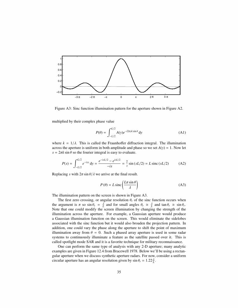
name.PRM Ascii file generated by the pre-processing software. It contains all theinformation needed to focus and align a single look complex (SLC) image witha master image. This file contains all the important SAR and InSAR processingparameters and is more completely described in Appendix B.

name.LED Ascii file generated by the pre-processing software to contain the orbitalinformation as a state vector.

name.raw File contains the raw signal data. Each row of signal data has a 412 byteheader record containing timing and other information followed by the radarecho stored as unsigned 2-byte complex numbers (1 byte real and 1 byte imagi-nary).

name.SLC File contains the focused single look complex (SLC) image. The signed4-byte complex numbers are stored as unsigned short integers (2-bytes real and2-bytes imaginary). The numbers are scaled to utilize the full dynamic range ofa short integer. (An 8-byte complex output option is also provided by the SARprocessor.)

trans.dat File contains the mapping between range, azimuth coordinates and longi-tude, latitude, topography coordinates. The topography is calculated with respectto a local spherical approximation to the earth (Appendix C) and therefore largenegative and positive numbers are possible.

The format is: range azimuth topography longitude latitude and numbers arestored as double precision floating point.

11

11301.587587 18451.999997 -272.883315 -115.156667 32.37333311308.909450 18451.999997 -273.413527 -115.156111 32.373333

topo ra.grd Grid of range, azimuth, and topography.

real.grd or imag.grd Grids of range, azimuth, and the real or imaginary part of thecomplex interferogram (files are deleted when no longer needed).

phase.grd Grid of range, azimuth, and interferometric phase modulus 2π.

corr.grd Grid of range, azimuth, and interferometrric coherence (0-1.)

xphase.grd Grid of range, azimuth, and phase gradient in the range direction in unitsof radians per pixel (optional).

yphase.grd Grid of range, azimuth, and phase gradient in the azimuth direction inunits of radians per pixel (optional).

mask.grd Grid of range, azimuth, and NaN or 1. NaN signifies data should bemasked.

unwrap.grd Grid of unwrapped interferometric phase in radians (optional).

All the files with suffix .grd are in NetCDF format. When the interferometric productshave been transformed back to geographic coordinates the file names include an ll.For example, phase ll.grd is a netcdf file of longitude, latitude, and interferometricphase modulus 2π.

Files having a .ps suffix are postscript plots of the quantity.For example, phase mask ll.ps is a postscript plot of masked phase in geographic co-ordinates.

Files having a .kml/png suffix are Google Earth images.For example, phase mask ll.kml/png is a Google Earth image of masked phase in geo-graphic coordinates.

(Note that the GMT command grd2xyz phase.grd -Zf > phase will produce a flat file offloats with a size of 4 ∗ nrow ∗ ncol bytes.)

2.2 Software DesignThe overall design of the software is illustrated in Figure 2. There is a set of preprocessingcode for each of the satellites. Example data sets are available at http://topex.ucsd.edu/gmtsar. Data, leader, and orbit files provided by the space agency are normally inCEOS format and are converted into generic *.raw and *.PRM files. The pre-processingcode checks for missing lines in the CEOS data file and aligns the radar echoes on a commonnear range or sample window start time (SWST). The output is a raw file (*.raw) that isready to be focused in the SAR processor. The relevant parameters are extracted from thevarious leader and orbit files and used to prepare a parameter file (*.PRM) as fully describedin Appendix B. After selecting the master image, a user-supplied topography grid of the area(dem.grd) is projected into radar coordinates to create a transformation file (trans.dat).

12

. . .ERS2_preproc ENVI_preproc ALOS_preprocC-code, csh C-code, csh C-code

GMTSARC-code

GMTSARcsh - GMT

libgmt

libnetcdfdisplay softwarePreviewGoogle Earthnvciew, matlab,IDL, . . .

.

libfftw

*.PRM*.rawtrans.dat

*.PRM*.SLC*.grdtrans.dat

Figure 2: Design of GMTSAR and preprocessors.

The GMTSAR code is the same for all the satellite data types. There are 4 essen-tial programs written in C called esarp, xcorr, phasediff, conv. The programs esarp andxcorr make extensive use of a 1-dimensional fast fourier transform (FFT) routine built intoGMT. In the original GMTSAR codes, the user needed to select the most appropriate FFTcode for optimal performance. That task is now done automatically done during the in-stallation of GMT5. The three options are: the default option uses FFT routines fromfftpack.c code (Swarztrauber 1982); the fastest option uses the Accelerate Framework in-cluded in the Mac OS X system; the third option uses the fftw code that is distributed byhttp://www.fftw.org/. The optimized FFT codes will reduce the runtime of these pro-grams by about 20-40%. The programs phasediff, and conv read/write GMT grd-files innetcdf format and therefore require that the user link with the libraries libgmt.a and lib-netcdf.a. These programs, as well as many standard GMT routines, are called from shellscripts. A list of the current scripts is found by executing the command gmtsar.csh.

13

align.csh align a pair of SAR images

align batch.csh align a stack of SAR images

align tops.csh geometric alignment of TOP-mode data

baseline table.csh make baseline vs time table

cleanup.csh cleanup the directories

dem2topo ra.csh transform a dem into range and azimuth coordinates

filter.csh filter the interferogram and make amp, phase and corr

fitoffset.csh solve for the affine parameters

geocode.csh convert range/azimuth to lon/lat

grd2kml.csh make a kml file for google earth

intf.csh make the interferogram from a single pair of SLCs

intf batch.csh make interferograms for a set of aligned SLCs

make a offset.csh make azimuth offsets

make dem.csh construct a dem from tiles

pre proc.csh preprocess the raw SAR data for a pair of images

pre proc batch.csh preprocess raw SAR data for a stack of images

p2p SAT.csh process an SAT interferogram from end-to-end (many p2p scripts)

proj ll2ra.csh project a grd file from lon/lat to range/azimuth

proj ll2ra ascii.csh project points from lon/lat to range/azimuth

proj ra2ll.csh project a grd file from range/azimuth to lon/lat

proj ra2ll ascii.csh project points from range/azimuth to lon/lat

sarp.csh focus a single SAR image

slc2amp.csh make a amplitude image from a SLC

snaphu.csh unwrap phase using snaphu

stack.csh compute mean and standard deviations of a stack of images

update PRM.csh replace a value in a PRF-file

Executing one of the commands will provide its usage:% sarp.cshUsage: sarp.csh file.PRMExample: sarp.csh IMG-HH-ALPSRP049040660-H1.0 A.PRM

3 Processing ExamplesThe modules of the GMTSAR package can be connected in a variety of ways to do special-ized SAR and InSAR processing. The foundation of the code is all optimized, written in C,and we hope is functionally stable. For example, the SAR processor esarp.c has remainedstable for more than a decade. We expect this C-code as well as the GMT code, will bestable on a time frame of years. New preprocessor code will need to be written as newsatellite data becomes available but everything downstream should not change significantly.

14

The flexible aspect of the package is the c-shell scripts to perform different types of InSARprocessing. Indeed, c-shell is not a particularly good language for writing large scripts andwe hope this part of the system will evolve based on input from knowledgeable users. Sofar we have developed three standard InSAR recipes. They are 2-pass processing, stackingfor time series analysis, and ScanSAR to strip-mode interferometry. We will outline theprocessing stages in these three examples. The first example is also used for testing theinstallation (Appendix G) so we will step through the InSAR processing for a pair of ALOSSAR images spanning the 2010 M7.2 Baja, Mexico Earthquake.

3.1 Two-pass processingA common approach to InSAR processing is to form an interferogram using two SAR im-ages and a digital elevation model. A flow diagram of a script called p2p SAT.csh is shownin Figure 3. Selecting a pair of images having the desired perpendicular baseline and timespan characteristics is an important issue that will be discussed in the next section understacking and time series. This example recovers the coseismic displacement from an earth-quake so the ALOS PALSAR images are selected as the pair spanning the M7.2 Baja, Mex-ico Earthquake having the minimum time span. To prepare for the processing one needs togenerate a digital elevation grid of the area in longitude and latitude coordinates spanningan area greater than the SAR coverage (e.g., longitude -116.25 to -115.16 and latitude 32.16to 33.16). The heights should be referenced to the WGS84 ellipsoid and not the geoid. Thecommand make dem.csh will make the grid but only if it has access to the tiles of SRTMor ASTER topography data as well as the EGM96 geoid model. A topographic grid of anyland area can be created using the website http://topex.ucsd.edu/gmtsar. The userplaces this topography grid (dem.grd) in a directory called /topo and the two scenes of rawSAR data in L1.0 CEOS format in the directory called /raw. The first scene is the referenceimage and the second scene is the repeat image. (Later when discussing the alignment oflarge stacks of SAR images we will use additional terminology of a single master image andmany slave images.) After modifying a file called configure.txt the user uses the commandp2p ALOS.csh IMG-HH-ALPSRP207600640-H1.0 A IMG-HH-ALPSRP227730640-H1.0 A configure.txtand waits for the results.

15

preprocess

focus

align

interfere

filter/snaphu

geocode

xcorr

phasediff

ref.PRM ref.raw

rep.PRM rep.raw

rep.CEOS

ref.CEOS dem.grd

rep.SLC0

rep.SLC

ref.SLC

topo_ra.grd

real.grd imag.grd

amp.grd phase.grd corr.grd

unwrap.grd xphase.grd yphase.grd

amp_ll.grd phase_ll.grd corr_ll.grd

unwrap_ll.grd xphase_ll.grd yphase_ll.grd

dem2topophase

Figure 3: Flow diagram of 2-pass processing beginning with raw SAR and orbital dataand a digital elevation grid (dem.grd) and ending with geocoded grids of interferomet-ric products.

An overview of the 7 main processing steps is shown in Figure 3 and the modules areprovided in Table 3. The first step is to preprocess raw SAR data and orbital information,usually in L1.0 CEOS format, to create an ascii parameter file (e.g. Table B1) and a rawdata file (e.g., Figure B3). This preprocessing involves specialized code to extract orbitalposition and velocity information from the leader files, align the raw radar echoes on acommon near range, and estimate the Doppler centroid of the raw data. The second step is tofocus each image to create two single look complex images as described in Appendix B. Thethird step is to align the repeat image to the reference image. This is accomplished by firstusing the orbital information to estimate the shift in range and azimuth needed to align theupper left corner of the images. Then many small patches (e.g., 64x64) are extracted fromeach image and cross correlated to determine 6 affine parameters needed to warp the repeatimage to match the second image. The repeat image is refocussed using these 6 parameters

16

resulting in sub-pixel alignment between the reference and repeat images. Smaller scalepixel shifts due to large amplitude surface topography are corrected at the interfere step.The fourth step (dem2topo ra) is to transform the digital elevation model from longitude,latitude, and topography into range, azimuth, and topography. This is done using the preciseorbital information of the reference image. Sometimes a -1 pixel range shift (i.e., derivedfrom a cross correlation between the amplitude image of the master and the range gradientof the topographic phase, offset topo is needed to improve the alignment. The fifth step isto interfere the reference and repeat SLC’s using the topo shift.grd to both refine the imagealignment of the repeat image due to topography parallax, and to remove the baseline-dependent topographic phase from the repeat image prior to cross multiplication (phasediff).Thus all the position and phase corrections are applied at the full resolution of the SLC’s.The sixth step filter/snaphu is to low-pass filter (conv) and decimate (4 in azimuth and 1 or2 in range) the real and imaginary components of the interferogram and compute standardproducts of amplitude, phase, and coherence. The Gaussian filter wavelength is selected bythe user in the config.txt file. A second set of filtered interferograms is also created usinga modified Goldstein filter algorithm (phasefilt) (Goldstein and Werner 1997; Baran et al.2003). Optionally one can compute unwrapped phase using the snaphu program of Chenand Zebker (Chen and Zebker 2000) as well as phase gradients Sandwell and Price 1998 inthe range (xphase) and azimuth (yphase) directions. To this point all the processing is donein the radar coordinates where the spacing of the range pixels before decimation is cτ/2 andthe spacing of the azimuth pixels before decimation is V/PRF. These parameters can befound in the parameter files (See Appendix B).

The final step is to geocode all the products by transforming from the range/azimuthcoordinate system of the master image to longitude and latitude. The c-shell scripts alsoproduce postscript images and kml-images of relevant products using the capabilities ofGMT. An image of the sample interferogram superimposed on the dem is shown in Figure 4.

17

Figure 4: Interferometric phase for an ascending track (T211, F0640) of ALOS PAL-SAR data over the April 4, 2010, El Major-Cucapah earthquake, Baja Mexico. Onefringe represents 11.8 cm displacement away from the radar. The phase is super-imposed on the gradient of the topography and other components such as faults andearthquake epicenters are easily added.

3.2 Stacking for time seriesA second common approach to InSAR processing is to form a time series of deformationfrom a stack of images. There are a variety of methods ranging from averaging to smallbaseline subsets to time series to persistent scattering. The practical, and sometimes mostchallenging issue related to these approaches is to geometrically align a large stack of im-ages and align this stack with a topographic phase model. (Note a new purely geometricapproach to image alignment is presented in Appendix E.) A diagram of a stack of SAR im-ages is shown in Figure 5. To achieve interferometric phase coherence, the alignment musthave subpixel accuracy in the radar coordinates of range and azimuth. In addition, thereshould be greater than 20% overlap in the Doppler centroid or bursts in ScanSAR images.We use the terminology that many slave images are geometrically aligned with one masterimage. Once the alignment is done, an interferogram can be constructed from any pair ofimages in the stack. We use the terminology of reference and repeat images for the first andsecond acquisition of the interferometric pair, respectively.

18

1 – preprocess update PRM.csh

ALOS pre process.csh

pre proc.csh ALOS fbd2fbs.c

ALOS fbs2fbd.c

2 – align and focus sarp.csh esarp.c

SAT baseline.c

align.csh xcorr.c

fitoffset.csh trend2d.c

3 – topo ra grd2xyz.c

SAT llt2rat.c

dem2topo ra.csh blockmedian.c

surface.c

topo2phase.c

grdimage.c

4 – interfere and filter SAT baseline.c

phasediff.c

intf.csh conv.c

filter.csh grdmath.c

grdimage.c

phasefilt.c

5 – unwrap phase grdcut.c

grdmath.c

snaphu.csh grd2xyz.c

snaphu.c

xyz2grd.c

grdimage.c

6 – geocode grdmath.c grd2xyz.c

proj ra2ll.csh gmtconvert.c

geocode.csh blockmedian.c

surface.c

grdtrack.c

grd2kml.csh grdimage.c

ps2raster.c

Table 3: Algorithm and codes for 2-pass processing – p2p SAT.csh

GMTSAR commands are italic. black: c-shell script, red: GMTSAR C-code, blue: GMT C-code, green:snaphu phase unwrapper (Chen and Zebker 2000).

Note this example if for processing an ALOS interferogram. For another satellite (e.g. Envisat) replace thecharacters ALOS by ENVI. Also note TOPS-mode data are processed slightly differently since the align.cshstep is performed using orbital data rather than xcorr and fitoffset.

19

azim

uth

time

master SLC

slave(s) SLC

known phasefrom DEM

range

Figure 5: Schematic diagram of a stack of SAR images and a topographic phase image.

Image alignment is problematic if the perpendicular baseline between the master imageand one of the slave images is greater than about 3/4 of the critical baseline because theimages will be baseline decorrelated (Appendix C). Temporal decorrelation can also occurwhen the scattering surface of the earth changes between the master and slave acquisitionsbecause of vegetation, snow, or other small-scale surface disturbances. As discussed above,our image alignment algorithm begins with a guess at the range and azimuth shift based onthe precise orbit and then uses 2-dimensional cross correlation on small patches. If thereare no areas in the images that are correlated then this cross correlation approach can failto achieve subpixel correlation. A plot of perpendicular baseline versus time can be used toidentify images that lie far from the master and therefore may not be suitable for subpixelalignment. An example of a baseline vs. time plot for an ALOS stack (Track 213, Frame0660, Coachella Valley, California) is shown in Figure 6. Temporal decorrelation is less ofan issue in this desert area. However in this case the baseline of ALOS drifts by more than5 km over a time span of 2 years. The critical baseline for the lower bandwidth (FBD) datais 6 km so, for example the acquisition on orbit number 12285 lies more than 4 km fromacquisition on orbit 13627.

20

primary match

secondary match23692

tertiary match

Figure 6: Baseline versus time plot partly created by the pre proc batch.csh command.Colored dots were added by user and represent the intended primary (red), secondary(yellow) and tertiary (green) image alignment. The grey lines were added and representcandidate interferograms. The interferometric pair marked by a blue line is used inAppendix C for assessing the accuracy of the earth curvature and topographic phasecorrections.

We perform the image alignment using the following steps:

1. Preprocess all the images independently and examine the PRM files for median valuesof Doppler centroid (fd1), near range (near range), and earth radius (earth radius). Anexample command is:

ALOS pre process IMG-HH-ALPSRP022200660-H1.0 A LED-ALPSRP022200660-H1.0 A

In this case there are 27 images so one creates a script to pre-process all 27 images.

2. Based on this analysis one preprocesses all the images using the batch processing com-mand.

pre proc batch.csh ALOS data.in

The file data.in defines the zero-baseline image and the common parameters for thestack.

IMG-HH-ALPSRP055750660-H1.0 A -near 846567 -radius 6371902.401705 -fd1 100IMG-HH-ALPSRP022200660-H1.0 AIMG-HH-ALPSRP028910660-H1.0 AMG-HH-ALPSRP035620660-H1.0 A

This command will also create a baseline versus time plot as shown in Figure 6.

21

3. The next step is to select the master image somewhere in the center of the baseline versustime plot. The objective in this case is to form long time span interferograms havingrelatively short baselines so the user connects candidate interferograms as shown in thegrey lines on Figure 6. The correlation of an interferogram deteriorates as the imagealignment degrades so optimally one would cross correlate each interferometric pair.However, since we would like to be able to stack interferograms and apply a uniformtopographic phase correction it is advantageous to have all the images in the stack atleast crudely (< 2 pixels) aligned. In this case we only plan to make interferogramsamong images that are nearby in baseline so image alignment only needs to be accuratelocally. Our approach is to have a multi-step alignment process where a set of imagesnear the master in baseline vs. time space are aligned directly to the master (primarymatch red dots in Figure 6). Once this set is aligned we can treat them each as surrogatemasters and align images on the periphery of the baseline versus time plot to one of thenearby surrogates. We call this a secondary match (yellow dots in Figure 6). For imagesvery far from the master we can perform a tertiary match.

4. The user puts this alignment information into a file align.in an executes the command:

align batch.csh ALOS align.in

All of the information on primary, secondary, and tertiary alignment is contained in thealign.in file which is constructed by the user based on the baseline versus time plot. Theexample for the set shown in Figure 6 follows.

IMG-HH-ALPSRP055750660-H1.0 A:IMG-HH-ALPSRP028910660-H1.0 A:IMG-HH-ALPSRP055750660-H1.0 AIMG-HH-ALPSRP055750660-H1.0 A:IMG-HH-ALPSRP035620660-H1.0 A:IMG-HH-ALPSRP055750660-H1.0 AIMG-HH-ALPSRP055750660-H1.0 A:IMG-HH-ALPSRP042330660-H1.0 A:IMG-HH-ALPSRP055750660-H1.0 AIMG-HH-ALPSRP055750660-H1.0 A:IMG-HH-ALPSRP049040660-H1.0 A:IMG-HH-ALPSRP055750660-H1.0 AIMG-HH-ALPSRP055750660-H1.0 A:IMG-HH-ALPSRP062460660-H1.0 A:IMG-HH-ALPSRP055750660-H1.0 AIMG-HH-ALPSRP055750660-H1.0 A:IMG-HH-ALPSRP075880660-H1.0 A:IMG-HH-ALPSRP055750660-H1.0 AIMG-HH-ALPSRP055750660-H1.0 A:IMG-HH-ALPSRP082590660-H1.0 A:IMG-HH-ALPSRP055750660-H1.0 AIMG-HH-ALPSRP055750660-H1.0 A:IMG-HH-ALPSRP089300660-H1.0 A:IMG-HH-ALPSRP055750660-H1.0 AIMG-HH-ALPSRP055750660-H1.0 A:IMG-HH-ALPSRP096010660-H1.0 A:IMG-HH-ALPSRP055750660-H1.0 AIMG-HH-ALPSRP055750660-H1.0 A:IMG-HH-ALPSRP129560660-H1.0 A:IMG-HH-ALPSRP055750660-H1.0 AIMG-HH-ALPSRP055750660-H1.0 A:IMG-HH-ALPSRP163110660-H1.0 A:IMG-HH-ALPSRP055750660-H1.0 AIMG-HH-ALPSRP055750660-H1.0 A:IMG-HH-ALPSRP183240660-H1.0 A:IMG-HH-ALPSRP055750660-H1.0 AIMG-HH-ALPSRP055750660-H1.0 A:IMG-HH-ALPSRP189950660-H1.0 A:IMG-HH-ALPSRP055750660-H1.0 AIMG-HH-ALPSRP049040660-H1.0 A:IMG-HH-ALPSRP022200660-H1.0 A:IMG-HH-ALPSRP055750660-H1.0 AIMG-HH-ALPSRP049040660-H1.0 A:IMG-HH-ALPSRP142980660-H1.0 A:IMG-HH-ALPSRP055750660-H1.0 AIMG-HH-ALPSRP049040660-H1.0 A:IMG-HH-ALPSRP149690660-H1.0 A:IMG-HH-ALPSRP055750660-H1.0 AIMG-HH-ALPSRP049040660-H1.0 A:IMG-HH-ALPSRP156400660-H1.0 A:IMG-HH-ALPSRP055750660-H1.0 AIMG-HH-ALPSRP075880660-H1.0 A:IMG-HH-ALPSRP196660660-H1.0 A:IMG-HH-ALPSRP055750660-H1.0 AIMG-HH-ALPSRP082590660-H1.0 A:IMG-HH-ALPSRP210080660-H1.0 A:IMG-HH-ALPSRP055750660-H1.0 AIMG-HH-ALPSRP096010660-H1.0 A:IMG-HH-ALPSRP109430660-H1.0 A:IMG-HH-ALPSRP055750660-H1.0 AIMG-HH-ALPSRP096010660-H1.0 A:IMG-HH-ALPSRP116140660-H1.0 A:IMG-HH-ALPSRP055750660-H1.0 AIMG-HH-ALPSRP096010660-H1.0 A:IMG-HH-ALPSRP122850660-H1.0 A:IMG-HH-ALPSRP055750660-H1.0 AIMG-HH-ALPSRP096010660-H1.0 A:IMG-HH-ALPSRP223500660-H1.0 A:IMG-HH-ALPSRP055750660-H1.0 AIMG-HH-ALPSRP096010660-H1.0 A:IMG-HH-ALPSRP230210660-H1.0 A:IMG-HH-ALPSRP055750660-H1.0 AIMG-HH-ALPSRP022200660-H1.0 A:IMG-HH-ALPSRP136270660-H1.0 A:IMG-HH-ALPSRP055750660-H1.0 A

The first image is the name of the master or surrogate master, the second image is theslave to be aligned, and the third image is the supermaster that is common to all images.Note that the order of the alignment is sometimes important since the surrogate masterneeds to be aligned to the master before it can serve as a surrogate. Aligning a stack of

22

27 images can take quite a bit of computer time so it is best to do this is a batch modeand head home for the evening.

5. While waiting for the image alignment, one can construct the topographic phase usingthe master image. Generate a dem.grd using the web site (http://topex.ucsd.edu/gmtsar) and place it in a subdirectory /topo at the same level as /raw and /SLC.

6. Make a set of interferograms using the command

int batch.csh ALOS intf.in intf.config

The an example file for intf.config can be copied from the location

GMTSAR/gmtsar/csh/example.intf.config

and edited for this particular data set. The file intf.in contains a list of the interferometricpairs. In this case we make 22 interferograms (Figure 7).

IMG-HH-ALPSRP022200660-H1.0 A: IMG-HH-ALPSRP136270660-H1.0 AIMG-HH-ALPSRP028910660-H1.0 A: IMG-HH-ALPSRP163110660-H1.0 AIMG-HH-ALPSRP035620660-H1.0 A: IMG-HH-ALPSRP183240660-H1.0 AIMG-HH-ALPSRP035620660-H1.0 A: IMG-HH-ALPSRP189950660-H1.0 AIMG-HH-ALPSRP042330660-H1.0 A: IMG-HH-ALPSRP196660660-H1.0 A

23

Figure 7: Twenty-two interferograms of a small area in Coachella Valley where groundsubsidence is prominent. Cold color denotes ground moves away from the radar. Colorscale saturates at +/- 10 cm. A linear trend was removed from each interferogram.Projection is radar coordinates.

24

Figure 8: Stack of 22 interferograms spanning a total interval of 48 years. Contoursare 1 cm/yr LOS displacement toward radar (mostly vertical in this case). (left) radarcoordinates and (right) geographic coordinates. The command grd2kml.csh is used tocreate a kml-file for Google Earth. Subsidence rates exceeding 4 cm/y occur in PalmDesert, Indian Wells, and La Quinta areas due to groundwater pumping (Sneed, Brandt,and Solt 2014).

7. Use SBAS to make a time series

sbas intf.tab scene.tab 88 28 700 1000 -smooth 1

For this example the user has prepared 88 files of unwrapped phase as well as 88 files ofcoherence derived from 28 SAR images. Each file has 700 columns and 1000 rows. Theuser must also prepare the intf.tab and scene.tab files as follows.

intf.tab(format: unwrap.grd corr.grd ref id rep id B perp)cut 02220 13627.grd corcut 02220 13627.grd 02220 13627 -19.387899cut 02891 03562.grd corcut 02891 03562.grd 02891 03562 369.671332cut 02891 04904.grd corcut 02891 04904.grd 02891 04904 -496.279669cut 02891 05575.grd corcut 02891 05575.grd 02891 05575 627.184879cut 02891 16311.grd corcut 02891 16311.grd 02891 16311 6.788277cut 02891 18324.grd corcut 02891 18324.grd 02891 18324 348.590674

scene.tab(format: scene id number of days)02220 17602891 22203562 26804233 31404904 36005575 406

The output is 28 files of displacement time series disp ##.grd in mm as well as a singlemean velocity vel.grd in mm/yr.

25

3.3 ScanSAR Interferometry

(These notes are ONLY for ALOS-1 ScanSAR. ALOS-2 ScanSAR and Sentinel-1 wideswath data are supplied as SLCs and can be treated just like normal swath-mode data soyou can probably skip this section.)

GMTSAR can perform two types of ScanSAR interferometry as more fully describedin Appendix D. ScanSAR to ScanSAR interferometry is possible when the reference andrepeat bursts overlap by more than about 20% but one must be very lucky to have morethan 20% overlap. The second approach, that is always possible, is ScanSAR to strip modeinterferometry. The only difference between Scan to strip processing and strip to stripprocessing is the preprocessing steps to convert one of the subswaths of the ScanSAR datainto a file that looks like a standard strip-mode raw data file. Here we provide a step-by-step example of processing a ScanSAR to strip (FBD) interferogram over Los AngelesBasin (Figure 9). This interferogram has a perpendicular baseline of 108 m and time spanof 184 days. The track number is 538 and the frame number is 2930 for FBD and 2950 forScanSAR.

Figure 9: Location of ALOS Scansar and FBD acquisition over Los Angeles for track538. Subswath 4 (SW4) has the same look angle as standard strip-mode data and alsoa similar PRF.

The processing steps are:

1. Preprocessing FBD raw data is done by ALOS pre process. Unlike the above case wherewe convert all the lower bandwidth (FBD) data to the higher bandwidth (FBS) mode,we keep the strip data in the FBD mode because this matches the bandwidth of theScanSAR data. Preprocessing a subswath of ScanSAR raw data is done using the pro-gram ALOS pre process SS. This preprocessor has many options as shown next.

26

SW1 SW2 SW3 SW4 SW5

near range (m) 730097 770120 806544 848515 878195

PRF (Hz) 1692 2370 1715 2160 1916

nburst 247 356 274 355 327

∆t(s) 0.146 0.150 0.160 0.164 0.171

nsamples 4976 4720 5376 4432 4688

off nadir (deg) 20.1 26.1 30.6 34.1 36.5

Table 4: Nominal radar parameters for each ScanSAR sub swath. The number ofechoes in a burst nburst is the only fixed parameter.

% ALOS pre process SS

Usage: ALOS pre process SS imagefile LEDfile [-near near range] [-radius RE] [-swath swath#] [-burst skip] [-num burst] [-swap] [-V] [-debug] [-quiet]

creates data.raw and writes out parameters (PRM format) to stdout

imagefile ALOS Level 1.0 complex file (CEOS format):

LEDfile ALOS Level 1.0 LED file (CEOS leaderfile format):

options:-near near range specify the near range (m)-radius RE specify the local earth radius (m)-swath specify swath number 1-5 [default 4]-burst skip number of burst to skip before starting output (1559 lines/burst)-num burst number of burst to process [default all]

there are 72 bursts in a WB1 frame-swap do byte-swap (should be automatic)-fd1 [DOPP] sets doppler centroid [fd1] to DOPP-V verbose write information)-debug write even more information-quiet don’t write any information

Example:

ALOS pre process SS IMG-HH-ALPSRS049842950-W1.0 D LED-ALPSRS049842950-W1.0 D-near 847916 -radius 6371668.872945 -burst skip 5 -num burst 36

burst # look angle #lines burst1 20.1 2472 26.1 3563 30.6 2744 34.1 3555 36.5 327

By default the ALOS pre process SS uses subswath 4, which naturally overlaps theswath mode imagery along the same track. The num burst parameter represents thenumber of burst that will be extracted from a long subswath of ScanSAR. The burst skipparameter controls the number of burst to skip before preprocessing raw data and it isdetermined by trial and error. After PRM files of both the ScanSAR mode and FBDmode are generated, the user runs ALOS baseline to see if the ashift value is reasonable.

27

If not, the user chooses another burst skip parameter and repeats this process until thea shift is less than 1703. For this LA example the following command was used.

ALOS pre process SS IMG-HH-ALPSRS049842950-W1.0 D LED-ALPSRS049842950-W1.0 D-nodopp -near 847916 -radius 6371729.321330 -num burst 18 -burst skip 5

Note that 18 bursts were extracted which will match the length of a single FBD frame.As described above frame-by-frame processing is usually more reliable than processingvery long swaths. The ALOS pre process SS terminates when it reaches the end of thedata file or the PRF changes in any of the subswaths. With some experimentation onecan set the burst skip to skip over the PRF change and start a fresh swath.

2. As described in Appendix D, the ALOS pre process SS simply inserts zero for the themissing lines in each subswath to create a standard strip-model file. To achieve optimalcorrelation between the scan and strip combination, one needs to zero the matchinglines in the FBD data (Bertran-Ortiz and Zebker 2007). This step is performed by theALOS fbd2ss which simply replaces real data with zeroes! The next task is to determinewhere to insert the zeros into the FBD data. Two parameters are needed to accountfor the shift and stretch between the two acquisitions. The ashift is the azimuth shiftneeded to align the first row of the FBD raw data to the subswath of ScanSAR data andthe a stretch a accounts for the PRF difference. These parameters can be obtained byaligning the ScanSAR SLC with the FBD SLC images using align.csh. Essential (butnot complete) steps in this alignment are listed below to guide the reader.

update PRM.csh IMG-HH-ALPSRS049842950-W1.0 D SW4.PRM num valid az 10224(note that 10224 is the length of 6 bursts of length 1704)

update PRM.csh IMG-HH-ALPSRP076682930-H1.0 D.PRM num valid az 10224(use the same synthetic aperture length for the FBD.)

sarp.csh IMG-HH-ALPSRP076682930-H1.0 D.PRM IMG-HH-ALPSRP076682930 H1.0 D.SLC(focus the FBD)

sarp.csh IMG-HH-ALPSRS049842950-W1.0 D SW4.PRM IMG-HH ALPSRS049842950-W1.0 D SW4.SLC(focus the WB1)

ALOS baseline IMG-HH-ALPSRS049842950-W1.0 D SW4.PRM IMG-HH-ALPSRP076682930-H1.0 D.PRM(get a guess for the rshift and ashift to aligh the upper left corner of the FBD to the WB1. Update the ashift and rshiftin the PRM-file of the FBD image then do a cross correlation.)

xcorr IMG-HH-ALPSRS049842950-W1.0 D SW4.PRM IMG-HH-ALPSRP076682930-H1.0 D.PRM

fitoffset.csh freq xcorr.dat(find the exact ashift and a stretch a parameter for the zeroing program ALOS fbd2ss)

ALOS fbd2ss IMG-HH-ALPSRP076682930-H1.0 D.PRM IMG-HH-ALPSRP076682930-H1.0 D ss.PRM733 1704 0.00437308(finally do the zeroing ashift = 733, num valid az/6 , a stretch a)

Note the rshift and ashift of the IMG-HH-ALPSRP076682930-H1.0 D ss.PRM shouldbe reset to zero after ALOS fbd2ss.

3. After the ALOS fbd2ss the special preprocessing steps are completed, the data are pro-cessed as one would normally process two strip-mode acquisitions similar to the stepsfound in process2pass.csh. The essential (but not complete) steps are listed below. Notep2p SAT.csh can’t be used directly because of the non standard filenames; some creativescripting or links could fix solve this issue.

28

align.csh ALOS IMG-HH-ALPSRS049842950-W1.0 D SW4 IMG-HH-ALPSRP076682930-H1.0 D ss

dem2topo ra.csh master.PRM dem.grdintf.csh IMG-HH-ALPSRS049842950-W1.0 D SW4.PRM IMG-HH-ALPSRP076682930-H1.0 D ss.PRM –topotopo ra.grd

filter.csh IMG-HH-ALPSRS049842950-W1.0 D SW4.PRM IMG-HH-ALPSRP076682930-H1.0 D ss.PRMgauss alos 300m 2

geocode.csh 0.1

The processed interferogram is shown in Figure 10. To make the interferogram moreinteresting we did not apply the topographic phase correction. During this analysis we alsoprocessed a standard FBD to FBD interferogram. For these two interferograms of the samearea and about the same time interval, the average coherence of the ScanSAR to FBD inter-ferogram was lower (0.38) than the FBD to FBD interferogram (0.67). Therefore there arereally no advantages to ScanSAR to strip-mode interferometry except that it provides moreinterferometric opportunities in case of events. For ScanSAR processing we commonly usea longer wavelength filter (300 or 500 m) to improve the visibility of the fringes.

Figure 10: An example of ScanSAR to FBD mode interferogram over Los AngelesBasin where the topographic phase has not been removed.

ScanSAR to ScanSAR processing is very similar to the sequence described above al-though one must be lucky to find a pair having sufficient burst overlap. For each WB1 datafile one creates 5 independent interferograms for each of the 5 subswaths. As shown in 4,each subswath has a very different PRF so the interferograms are not easily mosaicked inthe radar coordinates. However, if the data are processed with a consistent earth radius, theinterferograms will abut seamlessly when they are projected back into geographic coordi-nates as shown in Figure 11.

29

Figure 11: Descending ScanSAR to ScanSAR interferogram spanning the Mw 7.92008 Wenchuan earthquake (11.8 cm per fringe). The interferogram consists of 5 sub-swaths across look direction that abut almost seamlessly with no position or phaseadjustment. The decorrelation in the mountainous area to the left of the red surfacerupture line is due to the rather long baseline (920m) and high relief.

AcknowledgementsGMTSAR was developed over a period of 19 years by many people. Howard Zebker pro-vided the original FORTRAN code for the SAR processor. Evelyn Price translated the SARprocessor into C which greatly simplified the code although the SAR focusing algorithmremained unchanged. Price and Sandwell expanded this into a complete InSAR packageby adding cross correlation and phase modules. Paul Jamason wrote the original preproces-sors for ERS (CCRS and DPAF). Remko Sharro’s (Delft University) getorb routines wereoriginally used to compute precise orbits for proper focus, geolocation, and baseline esti-mation. The GIPS package, written by Peter Ford at MIT, was used to develop an overallsystem called SIOSAR which remained stable for 11 years. Sean Buckley’s Envisat de-coder is used in the Envisat preprocessor. In 2010 the GIPS software was replaced by GMTmodules. Rob Mellors rewrote the ALOS preprocessing code developed by Sandwell intoa robust package which was later translated by Matt Wei into the ERS and ENVISAT pre-processors. Rob also wrote completely new software for image cross correlation as wellas for Goldstein/Werner interferogram filtering. Xiaopeng Tong did extensive testing and

30

refinement of the phase module to remove some of the approximations built into SIOSAR.He also developed the shell scripts for two-pass processing, stacking and the sbas C-code.The Snaphu phase unwrapping code, written by Chen and Zebker, is used without mod-ification in GMTSAR. Paul Wessel provided several enhancements to GMT to deal withprocessing of large binary tables. He also modified all of the code to interferace with GMTAPI routines during his sabbatical leave at Scripps. In addition he developed code to createkml output. GMTSAR makes extensive use of the GMT routines blockmedian and surfacewhich were developed by Walter Smith and Paul Wessel. These lie at the heart of the GMT-SAR algorithms for transforming between geographic and radar coordinates. We believethese routines are responsible for the ability of GMTSAR to maintain phase coherence inareas of rugged terrain where other InSAR packages sometimes fail. Kahlid Soofi sup-ported this effort through funding from Conoco/Phillips as well as testing and developmentof the software. Most recently Xiaohua Xu and Sandwell co-developed the pre-processingand alignment codes needed for TOPS-mode interferometry under the guidance of PabloGonzalez. Many users provided feedback and bug reports to achieve a relatively robust andstable set of software. The entire 19-year development was done as an effort to improve theresolution and accuracy of interferograms. Each iteration provided incremental improve-ments over the original Stanford/JPL code. The latest package was designed to move tothe next level of processing thousands of wide-swath interferograms with minimal humanintervention. San Diego State University and Scripps Institution of Oceanography providedsalary support for Mellors and Sandwell during the last 2 years of code development. Inaddition, Mellors was partially supported under the auspices of the U.S. Department of En-ergy by Lawrence Livermore National Laboratory under Contract DE-AC52-07NA27344.Recent development was supported by the NSF Geoinfomatics Program 1347204.

ReferencesBaran, I. et al. (2003). “A modification to the Goldsetin Radar interferogram filter.” In:

IEEE Trans. Geoscience Rem. Sens. 41.9, pp. 2114–2118.Bertran-Ortiz, A. and H. A. Zebker (2007). “ScanSAR-to-Stripmap Mode Interferom-

etry Processing Using ENVISAT/ASAR Data”. In: IEEE Trans. Geoscience Rem.Sens. 45.11, pp. 3468–3480.

Chen, C. and H. A. Zebker (2000). “Network approaches to two-dimensional phase un-wrapping: intractability and two new algorithms”. In: Journal of the Optical Societyof America A 17, pp. 401–414.

Curlander, J. C. and R. N. McDonough (1991). Synthetic Aperture Radar: Systems andSignal Processing. Chapter 4. New York City: John Wiley & Sons.

Farr, T.G. et al. (2004). “The Shuttle Radar Topography Mission”. In: Rev. Geophys.17. doi:10.1029/2005RG000183.

Goldstein, R.M. and C.L. Werner (1997). “Radar ice motion interferometry”. In: Proc.3rd ERS Symp. Vol. 2:11. Florence, Italy, pp. 969–972.

Press, W.H. et al. (1992). Numerical recipes in C. Second Edition. 994 pp. New YorkCity: Cambridge University Press.

Sandwell, D.T. and E.J. Price (1998). “Phase gradient approach to stacking interfero-grams”. In: J. Geophys. Res. 103, pp. 30183–30204.

Sneed, M. and J. Brandt (2007). Detection and Measurement of Land Subsidence UsingGPS Surveying and InSAR, Coachella Valley, California, 1996-2006. Tech. rep.2007-5251. New York City: USGS Scientific Investigations Report.

31

Sneed, M., J. Brandt, and M. Solt (2014). Land subsidence, groundwater levels, andgeology in the Coachella Valley, California, 1993-2010. Tech. rep. US GeologicalSurvey.

Swarztrauber, P.N. (1982). Vectorizing the FFTs, in Parallel Computations (G. Ro-drigue, ed.) Cambridge, MA: Academic Press, pp. 51–83.

Wessel, P. and W.H.F. Smith (1998). “New, improved version of Generic MappingTools released”. In: EOS Trans. Amer. Geophys. U. 79(47). 579 pp.

Wessel, P., W.H.F. Smith, et al. (2013). “Generic Mapping Tools: Improved versionreleased”. In: EOS Trans. Amer. Geophys. U. 94, pp. 409–410.

4 Problems1. Precise orbital information is used in 4 areas of InSAR processing. Describe the 4

uses.

2. The natural coordinates of a radar image have range or time along one axis andazimuth or slow time along the other axis. Why is the term slow time used?

3. Describe an algorithm to transform a point on the surface of the earth (longitude,latitude, elevation) into radar coordinates.

4. When a SAR image is focussed at zero Doppler, the radar coordinates of a pointreflector correspond to the minimum range. Why? Derive the equations (4) and(5) for adjusting the range and azimuth coordinates when an image is focussed at anon-zero Doppler.

5. GMTSAR uses a quadratic function to approximate the changes in baseline (hori-zontal and vertical) along the image frame. The quadratic formula is:

B (s) = a + bs + cs2

where s is slow time ranging from the start to the end of the frame [0,T ]. Supposethe actual baseline is measured at three times along the frame 0, T

2 ,T and the valuesare B1, B2, B3. Derive an expression for the parameters a, b, c. The forward model is

B1B2B3

=

1 0 01 T

2T 2

41 T T 2

a

bc

.

6. Satellite orbital information is commonly provided as state vectors of position andvelocity at regular intervals (e.g., 1 minute). Hermite polynomial interpolation isoften used to interpolate the orbit to the full sampling rate of the radar (e.g., 2000Hz). What are the strengths and weaknesses of this approach? (This may require aliterature search.)

7. Explain the terminology, master and slaves, reference and repeat.

32

A Principles of Synthetic Aperture Radar

A.1 IntroductionSynthetic aperture radar (SAR) satellites collect swaths of side-looking echoes at a suf-ficiently high range resolution and along-track sampling rate to form high resolutionimagery (see Figure A1). As discussed in this appendix, the range resolution of theraw radar data is determined by the pulse length (or 1/bandwidth) and the incidenceangle. For real aperture radar, the along-track or azimuth resolution of the outgoingmicrowave pulse is diffraction limited to an angle corresponding to the wavelength ofthe radar (e.g. 0.05 m) divided by the length of the aperture (e.g. 10 m). When thisbeam pattern is projected onto the surface of the earth at a range of say 850 km, it illu-minates 4250 m in the along-track dimension so the raw radar data are horribly out offocus in azimuth. Using the synthetic aperture method, the image can be focused on apoint reflector on the ground by coherently summing thousands of consecutive echoesthus creating a synthetic aperture perhaps 4250 m long. Proper focus is achieved bysumming the complex numbers along a constant range. The focused image containsboth amplitude (backscatter) and phase (range) information for each pixel.

Footprint

Swath

Look Angle

Radar Pulses

SAR Antenna

Sub-satellite ground track

Satellite trajectory

Figure A1: Schematic diagram of a SAR satellite in orbit. The SAR antenna has itslong axis in the flight direction also called the azimuth direction and the short axisin the range direction. The radar sends pulses to one side of the ground track thatilluminate the earth over a large elliptical footprint. The reflected energy returns to theradar where it is recorded as a function of fast time in the range direction and slow time,or echo number, in the azimuth direction.

33

A.2 Fraunhoffer diffractionTo understand why a synthetic aperture is needed for microwave remote sensing fromorbital altitude one must understand the concepts of diffraction and resolution. Con-sider the projection pattern of coherent radiation after it passes through an aperture(see Figure A2). First we’ll consider a 1-D aperture and then go on to a 2-D rectangu-lar aperture to simulate a rectangular SAR antenna. The 2-D case provides the shapeand dimension of the footprint of the radar. Although we will develop the resolutioncharacteristics of apertures as transmitters of radiation, the resolution characteristicsare exactly the same when the aperture is used to receive radiation. These notes weredeveloped from Rees 2001 and Bracewell 1978.

y

z

P

O

AL/2

-L/2

y sin

A

O

screen aperture

Figure A2: Diagram for the projection of coherent microwaves on a screen that is farfrom the aperture of length L.

We simulate coherent radiation by point sources of radiation distributed along theaperture between −L/2 and L/2. For simplicity we’ll assume all the sources have thesame amplitude, wavelength λ, and phase. Given these sources of radiation, we solvefor the illumination pattern on the screen as a function of θ. We’ll assume that thescreen is far enough from the aperture so that rays AP and OP are parallel. Laterwe’ll determine how far away the screen needs to be in order for this approximationto hold. Under these conditions, the ray AP is slightly shorter than the ray OP byan amount −y sin θ. This corresponds to a phase shift of −2π

λy sin θ. The amplitude

of the illumination at point P is the integral over all of the sources along the aperture

34

−3 −2 −π 0 π 2 3

−0.2

0

0.2

0.4

0.6

0.8

1

ππ π π

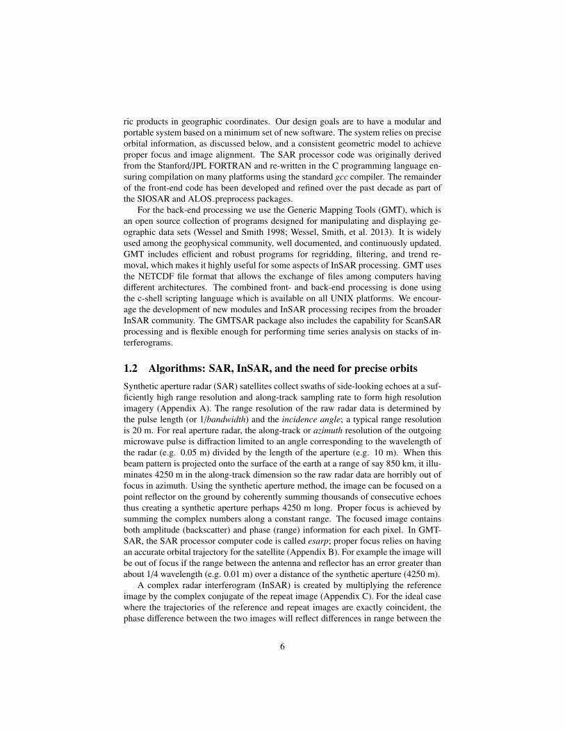
Figure A3: Sinc function illumination pattern for the aperture shown in Figure A2.

multiplied by their complex phase value

P(θ) =

∫ L/2

−L/2A(y)e−i2πyk sin θ dy (A1)

where k = 1/λ. This is called the Fraunhoffer diffraction integral. The illuminationacross the aperture is uniform in both amplitude and phase so we set A(y) = 1. Now lets = 2πk sin θ so the fourier integral is easy to evaluate.

P(s) =

∫ L/2

−L/2e−isy dy =

e−isL/2 − eisL/2

−is=

2s

sin (sL/2) = L sinc (sL/2) (A2)

Replacing s with 2π sin θ/λ we arrive at the final result.

P (θ) = L sinc(

Lπ sin θλ

)(A3)

The illumination pattern on the screen is shown in Figure A3.The first zero crossing, or angular resolution θr of the sinc function occurs when

the argument is π so sin θr = λL and for small angles θr �

λL and tan θr � sin θr.

Note that one could modify the screen illumination by changing the strength of theillumination across the aperture. For example, a Gaussian aperture would producea Gaussian illumination function on the screen. This would eliminate the sidelobesassociated with the sinc function but it would also broaden the projection pattern. Inaddition, one could vary the phase along the aperture to shift the point of maximumillumination away from θ = 0. Such a phased array aperture is used in some radarsystems to continuously illuminate a feature as the satellite passed over it. This iscalled spotlight mode SAR and it is a favorite technique for military reconnaissance.

One can perform the same type of analysis with any 2-D aperture; many analyticexamples are given in Figure 12.4 from Bracewell 1978. Below we’ll be using a rectan-gular aperture when we discuss synthetic aperture radars. For now, consider a uniformcircular aperture has an angular resolution given by sin θr = 1.22 λ

L .

35

H

D

D s

θr

Figure A4: Beam-limited footprint Ds of a circular aperture (radar altimeter or opticaltelescope) at an altitude of H.

The Geosat radar altimeter orbits the Earth at an altitude of 800 km and illuminatesthe ocean surface with a 1-m parabolic dish antenna operating at Ku band (13.5 GHz,θ = 0.022m) (Figure A4). The diameter of the beam-limited footprint on the oceansurface is Ds = 2H tan θr � 2.44H λ

D or in this case 43 km.An optical system with the same 1 m diameter aperture, but operating at a wave-

length of θ = 5 × 10−7 m, has a footprint diameter of 0.97 m. The Hubble space tele-scope reports an angular resolution of 0.1 arcsecond, which corresponds to an effectiveaperture of 1.27 m. Thus a 1-m ground resolution is possible for optical systems whilethe same size aperture operating in the microwave part of the spectrum has a 44,000times worse resolution. Achieving high angular resolution for a microwave system willrequire a major increase in the length of the aperture.

Before moving on to the 2-D case, we should check the assumption used in devel-oping the Fraunhoffer diffraction integral that the rays AP and OP are parallel. Sup-pose we examine the case when θ = 0; the ray path AP is slightly longer than OP(Figure A5). This parallel-ray assumption breaks down when the phase of ray path APis more than π/2 radians longer than OP which corresponds to a distance of λ

4 . Let’sdetermine the conditions when this happens.

The condition that the path length difference is smaller than 1/4 wavelength is[L2

4 + z2] 1

2− z < λ

4 (A4)

or can be rewritten as [(L2z

)2+ 1

] 12− 1 < λ

4z (A5)

Now assume L � z so we can expand the term in bracket in a binomial series.

1 + L2

8z2 − 1 < λ4z (A6)

36

and we find z f >L2

2λ where z f is the Fresnel distance. So when z < z f we are in the nearfield and we need to use a more rigorous diffraction theory. However when z � z f weare safe to use the parallel-ray approximation and the Fraunhoffer diffraction integralis appropriate. Next consider some examples:

Geosat: L = 1 m, λ = 0.022 m z f = 23 m

At an orbital altitude of 800 km the parallel-ray approximation is valid.

Optical telescope: L = 1 m, λ = 5 × 10−7 m z f = 4000 km.

So we see that an optical system with an orbital altitude of 800 km will require near-field optics.

What about a synthetic aperture radar (discussed below) such as ERS with a 4000 mlong synthetic aperture?

ERS SAR: L = 4000 m, λ = 0.058 m z f = 140, 000 km.

Thus near-field optics are also required to achieve full SAR resolution for ERS.This near-field correction is done in the SAR processor by performing a step calledrange migration and it is a large factor in making SAR processing so CPU-intensive.

A.3 2-D ApertureA 2-D rectangular aperture is a good approximation to a typical spaceborne strip-modeSAR. The aperture is longer in the flight direction (length L) than in the flight perpen-dicular direction (width W) as shown in Figure A6. As in the 1-D case, one uses a 2-DFraunhoffer diffraction integral to calculate the projection pattern of the antenna. Theintegral is

P(θx, θy

)=

∫ L/2

−L/2

∫ W/2

−W/2A(x, y) exp

[i 2πλ

(x sin θx + y sin θy

)]dx dy (A7)

where λ is the wavelength of the radar. As in the 1-D case we’ll assume the apertureA(x, y) has uniform amplitude and phase. In this case the projection pattern can be

z

L/2

L 2

4 + z 2

1/2

O

A

P

Figure A5: Diagram showing the increases length of path AP with respect to OP dueto an offset of L/2.

37

x

y

sinθ

ysinθ

x

W

L

λ/Lλ/W

Figure A6: Diagram showing the projection pattern (right) for a rectangular SAR an-tenna (left).

integrated analytically and is

P(θx, θy

)= LW sinc

(πW sin θx

λ

)sinc

(πL sin θy

λ

). (A8)

The first zero crossing of this 2-D sinc function is illustrated in Figure A6 (right).The ERS radar has a wavelength of 0.05 m, an antenna length L of 10 m, and an

antenna width W of 1 m. For a nominal look angle of 23◦ the slant range R is 850km. The footprint of the radar has an along-track dimension Da = 2Rλ/L, which is 8.5km. As discussed below this is approximately the length of the synthetic aperture usedin the SAR processor. The footprint in the range direction is 10 times larger or about85 km.

A.4 Range resolution (end view)The radar emits a short pulse that reflects off the surface of the earth and returns to theantenna. The amplitude versus time of the return pulse is a recording of the reflectivityof the surface. If adjacent reflectors appear as two distinct peaks in the return waveformthen they are resolved in range. The nominal slant range resolution is ∆r = Cτ/2 whereτ is the pulse length, C is the speed of light and θ is the look angle. The factor of 2accounts for the 2-way travel time of the pulse. Figure A7 shows how the ground rangeresolution is geometrically related to the slant range resolution Rr = Cτ

2 sin θ .Note the ground range resolution is infinite for vertical look angle and improves as

look angle is increased. Also note that the range resolution is independent of the heightof the spacecraft H. The range resolution can be improved by increasing the bandwidthof the radar. Usually the radar bandwidth is a small fraction of the carrier frequencyso shorter wavelength radar does not necessarily enable higher range resolution. In

38

H

Figure A7: Diagram of radar flying into the page emitting a pulse of length ρ. Thatreflects from two points on the surface of the earth.

many cases the bandwidth of the radar is limited by the speed at which the data can betransmitted from the satellite to a ground station.

A.5 Azimuth resolution (top view)To understand the azimuth resolution, consider a single point reflector on the groundthat is illuminated as the radar passes overhead (Figure A8). From the Fraunhofferdiffraction analysis we know the length of the illumination (twice the angular resolu-tion) is related to the wavelength of the radar divided by the length of the antenna. Asdiscussed above the along-track dimension of the ERS footprint is 8.5 km so the nom-inal resolution Ra is 4.25 km, which is very poor. This is the azimuth resolution of thereal-aperture radar

Ra = ρ tan θr �ρλ

L=

λHL cos θ

(A9)

where L is the length of radar antenna, ρ is the slant range, and λ is the wavelength ofthe radar.

If the scatterer on the ground remains stationary as the satellite passes overhead,then one can assemble a synthetic aperture with a length equal to the along-trackbeamwidth of length which is 2Ra. This much longer aperture of 8.5 km results ina dramatic improvement in azimuth resolution given by

R′

a =λρ

2Ra=

L2

(A10)

which is the theoretical resolution of a strip-mode SAR. Note the synthetic apertureazimuth resolution is independent of spacecraft height and improves as the antennalength is reduced. One could form a longer synthetic aperture by steering the transmit-ted radar beam so it follows the target as the spacecraft (aircraft) flies by. This is calledspotlight-mode SAR.

39

L

r

Ra

Figure A8: Top view of SAR antenna imaging a point reflector. The reflector remainswithin the illumination pattern over the real aperture length of 2Ra.

A.6 Range and Azimuth Resolution of ERS SARThe ERS SAR has a bandwidth of 15.6 MHz, an antenna length of 10 m and a lookangle of 23◦. Accordingly the ground range resolution is about 25 m and the maximumazimuth resolution is 5 m. In practice, one averages several “looks” together to improvethe quality of the amplitude (backscatter) image. In the case of ERS, one could average5 looks for a resolution cell of 25 m by 25 m.

A.7 Pulse repetition frequencyThe discussion above suggests that we should make the antenna length L as short aspossible to improve azimuth resolution. However, to form a complete aperture withoutaliasing longer wavelengths back into shorter wavelengths we must pulse the radar atan along-track distance of L/2 or shorter. To understand why such a rapid pulse rateis necessary, consider the maximum Doppler shift from a point that is illuminated ata maximum distance ahead of the radar (Figure A9) where vo is the carrier frequency= C/λ and V is the velocity of spacecraft relative to the ground.

The maximum Doppler shift occurs at a maximum angle of

sin θa =λ

L

∆ν = 2νoVC sin θa =

2Cλ

VCλ

L=

2VL

(A11)

This corresponds to a maximum along-track distance between samples of L/2. ForERS this corresponds to a minimum pulse repetition frequency (PRF) of 1400 Hz. Theactual PRF of ERS is 1680 Hz.

A.8 Other constraints on the PRFThe PRF cannot be too large or the return pulses from the near range and far range willoverlap in time as shown in Figure A10.

40

Figure A9: Diagram showing the angle between broadside to the antenna and the pointwhere a reflector first enters the illumination of the antenna.

Figure A10: End view of the distance to the near range and far range of the radarillumination pattern.

PRF <1

t2 − t1

t1 =2H

C cos θ1t2 =

2HC cos θ2

∆t =2HC

(sec θ2 − sec θ1)

2VL< PRF <

C2H

(sec θ2 − sec θ1)−1

(A12)

For ERS the look angles to the rear range and far range are 18◦ and 24◦, respectively.Thus the maximum PRF is 4777 Hz. The actual PRF of 1680 is safely below this valueand the real limitation is imposed by the speed of the data link from the spacecraft tothe ground. A wider swath or a higher PRF would require a faster data link than ispossible using a normal X-band communication link of 105 Mbps.

41

ReferencesBracewell, R.N. (1978). The Fourier Transform and Its Applications. Second Edition.

New York City: McGraw-Hill Book Co.Curlander, John C. and Robert N. McDonough (1991). Synthetic Aperture Radar: Sys-

tems and Signal Processing. Chapter 4. John Wiley & Sons.Rees, W.G. (2001). Physical Principles of Remote Sensing. Cambridge, UK: Cam-

bridge University Press.

A.9 Problems1. What is the illumination pattern for an aperture with a sign reversal at its center?

What is P(0)? Is the function real or imaginary? Is the function symmetric orasymmetric?

The aperture is

A(y) =

0 |y| > L

2

1 0 < y ≤ L2

−1 − L2 ≤ y < 0

2. (a) What is the illumination pattern for the aperture below?

(b) What is the illumination pattern in the limit as L1 approaches L2?

P( )

L1

L2

3. What is the theoretical azimuth resolution of a spotlight-mode SAR that canilluminate the target over a 10◦ angle as shown in the diagram below?

42

5˚ 5˚

4. Derive the projection pattern for a 2-D rectangular aperture of length L and widthW given in equation (A8).

5. What is the ground-range resolution of side-looking radar with a pulse length of6 × 10−8s and a look angle of 45◦?

6. (a) What is the period for a satellite in a circular orbit about the moon where theradius of the orbit is 1.9 × 106 m? The mass of the moon is 7.34 × 1022 kg.

(b) You are developing a SAR mission for the moon. The length of your SARantenna is 10 m. What minimum pulse repetition frequency is needed toform a complete aperture? The circumference of the moon is 1.1 × 107 m.You will need the orbital period from problem (a).

7. Derive equation (A10).

8. A SAR with a 10 m long antenna is orbiting the earth with a ground speed of7000 ms−1. What is the maximum possible swath width. Use a look angle to thenear range of 45◦ and assume the earth is flat.

9. CryoSat is a nadir-looking altimeter that uses a burst-mode synthetic aperture toreduce the length of the radar footprint in the along-track direction. The radar hasa pulse repetition frequency of 18 kHz and uses 64 echoes in one burst to formthe synthetic aperture. What is the along-track resolution of the footprint? Whatis the Fresnel distance for this configuration (ground track velocity 7000 ms−1,700 km altitude)?

43

B SAR Image Formation

B.1 Overview of the range-doppler algorithmFrom Curlander and McDonough 1991. The basic SAR theory is conceptually sim-ple (Appendix A) yet when one looks into the inner workings of the SAR processor itappears quite complicated. The most difficult part of the problem is related to the cou-pling between the azimuthal compression and the orbital parameters. In the old dayswhen the satellite orbits were not known very accurately, one would use techniquessuch as clutterlock and autofocus to derive the orbital parameters from the data. This isno longer necessary with the high accuracy orbits available today. A standard process-ing sequence follows where the first two steps are done on board the satellite while theremaining 4 steps are done by the user with a digital SAR processor. The discussionprovided here is for the ERS-1 satellite although the concepts translate to any modernstrip-mode SAR satellite.

B.2 Processing on board the satelliteDemodulate The electromagnetic wave consists of a chirp of bandwidth B (∼15 MHz)superimposed on carrier frequency ωo (∼5 GHz). To record the return signal, one couldsimply digitize the amplitude of the electric field E(t) at a sampling rate of 10 GHzusing 1-byte encoding. However, this would generate 10 Gbytes of data every second!We are really only interested in how the chirp has been delayed and distorted by thereflection off the Earth’s surface. The trick here is to use the shift theorem (Bracewell1978, p. 108) to isolate the 15 MHz part of the spectrum containing the chirp. Supposewe multiply the signal E(t) by ei2πωot. This will shift the Fourier transform of the signalas shown in Figure B1.

- o 0 o 2 o

Figure B1: Diagram showing the power spectrum of the radar signal before and aftershifting by the carrier frequency.

The function E(t) is a real-valued function so we know that its Fourier transformhas Hermitian symmetry about the origin, that is E(−ω) = E∗(ω). Because of thissymmetry, all of the information in the time series is contained within the bandwidth

44

of a single spectral peak. Next we low-pass filter the signal to isolate the spectral peakcentered at the zero frequency. The original signal E(t) was a real-valued function butafter this shift/filter operation the output complex. No information is lost in this processand now the output can be digitized at the much lower rate of twice the bandwidth ofthe chirp (∼30 MHz).

Digitize The complex signal is digitized at 5 bits per pixel so the numbers rangefrom 0 to 31; the mean value is 15.5. Digitizing the data at 8 bits per pixel wouldseem more convenient but transmitting these extra 3 bits to the ground receiving stationexceeds the bandwidth of the telemetry so every effort is made to compress the databefore transmission. Once the data are on the ground they are expanded to 8 bits (onebyte) for programming convenience. Engineers refer to the real and imaginary partsof the signal as the in-phase (I) and quadrature (Q) components. The raw signal filescontain rows of (11644 bytes) that represent a single radar echo (Figure B2). The first412 bytes are timing and other information while the remaining 11232 bytes containthe 5616 complex numbers of raw signal data.

Raw Signal Data

range

azimuth patch

incomplete aperture complete aperture incomplete aperture

412 bytes 11232 bytes – 5161 complex numbers timing raw signal data

Figure B2: Raw signal data

B.3 Digital SAR processingThe digital SAR processor is a computer program that converts the raw signal datainto a single-look complex (SLC) image. An overview is provided in Figure B3 this isfollowed by a detailed description of each step.

45

Digital SAR Processing Overview

(1) Range compression performed on each radar echo

(2) Patch processing of range-compressed echos

(3) Range migration performed on each pixel of range-compressed

data whose columns have been fourier transformed

(4) Azimuth compression performed on each column of range-

compressed, range-migrated data

Parameter

file

Single Look

Complex (SLC) image data file

Raw signal

data file

Figure B3: Digital SAR processing overview

46

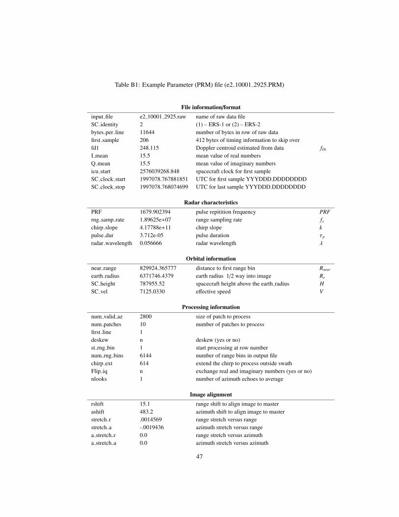
Table B1: Example Parameter (PRM) file (e2 10001 2925.PRM)

File information/formatinput file e2 10001 2925.raw name of raw data fileSC identity 2 (1) – ERS-1 or (2) – ERS-2bytes per line 11644 number of bytes in row of raw datafirst sample 206 412 bytes of timing information to skip overfd1 248.115 Doppler centroid estimated from data fDc

I mean 15.5 mean value of real numbersQ mean 15.5 mean value of imaginary numbersicu start 2576039268.848 spacecraft clock for first sampleSC clock start 1997078.767881851 UTC for first sample YYYDDD.DDDDDDDDSC clock stop 1997078.768074699 UTC for last sample YYYDDD.DDDDDDDD

Radar characteristicsPRF 1679.902394 pulse repitition frequency PRFrng samp rate 1.89625e+07 range sampling rate fs

chirp slope 4.17788e+11 chirp slope kpulse dur 3.712e-05 pulse duration τp

radar wavelength 0.056666 radar wavelength λ

Orbital informationnear range 829924.365777 distance to first range bin Rnear

earth radius 6371746.4379 earth radius 1/2 way into image Re

SC height 787955.52 spacecraft height above the earth radius HSC vel 7125.0330 effective speed V

Processing informationnum valid az 2800 size of patch to processnum patches 10 number of patches to processfirst line 1deskew n deskew (yes or no)st rng bin 1 start processing at row numbernum rng bins 6144 number of range bins in output filechirp ext 614 extend the chirp to process outside swathFlip iq n exchange real and imaginary numbers (yes or no)nlooks 1 number of azimuth echoes to average

Image alignmentrshift 15.1 range shift to align image to masterashift 483.2 azimuth shift to align image to masterstretch r .0014569 range stretch versus rangestretch a -.0019436 azimuth stretch versus rangea stretch r 0.0 range stretch versus azimutha stretch a 0.0 azimuth stretch versus azimuth

47

1. Range Compression A sharp radar pulse is recovered by deconvolution of thechirp. This is done with fast fourier transform. There are 5616 points in theERS-1 signal data and the chirp is 703 points long. Both are zero-padded to alength of 8192 prior to deconvolution to take advantage of the speed of the radix-2 fft algorithms. Later we keep 6144 points, which enables one to extract thephase beyond the edges of the original swath. Since the chirp really did interactwith the ground outside the digitized swath, this is not magic. The number 6144has small prime factors that may be optimal for later 2-D fft phase unwrappingalgorithms.

2. Patch Processing The next step is to focus the image in the along-track or az-imuth direction. This is also done by fft, but now we need to process columnsrather than rows. For the ERS radar, the synthetic aperture is 1296 points long sowe need to read at least that many rows into the memory of the computer. Actu-ally 4096 rows is better number since it is a power of 2. A typical ERS raw datafile has 28,000 rows so we will need to process many of these patches. One prob-lem with this approach is that the synthetic aperture is only complete for the inner2800 points of the 4096 data patch so the patches must have a 1296-point overlap(Figure B3). A 4096×5616 patch requires at least 184 Mbytes of computer mem-ory for single precision real numbers. In the old days before this large memoryspace was available, each patch was transposed—corner turning—using high-speed disks so the data could be processed on a column-by-column basis. TheL-band data from ALOS have a much longer synthetic aperture and patch size.Efficient processing of these data require a minimum of 2 Gbytes of computermemory.

3. Range Migration As we will see below, a point target will appear as a hyperbolic-shaped reflection as it moves through the synthetic aperture. In addition, therecould be a pronounced linear drift due to an elliptical orbit and earth rotation.In other words, the target will migrate in range cell as a linear trend plus a hy-perbola. The shape of this migration path is calculated from the precise orbitalinformation and is approximated by a parabola. Prior to focusing the imagealong a single column, these signals must be migrated back to a constant rangecell. This is called range migration and the fastest way to do this is by Fouriertransforming the columns first. Each Fourier component corresponds to a uniqueDoppler shift and also a unique value of range migration; for an ideal radar, thefirst component will have zero Doppler and will correspond to the point on theearth that is perpendicular to the spacecraft velocity vector. The second compo-nent will have a small positive Doppler shift and a small migration of the rangecells will be needed - and so on all the way through the positive and negativeDoppler spectrum.

4. Azimuth Compression The final step in the processing is to focus the data in az-imuth by accounting for the phase shift of the target as it moves through the aper-ture. In Appendix A, we calculated the illumination pattern on a screen due tothe propagation of a coherent wave from the aperture to the screen. The azimuthcompression relies on the same theory although we do the opposite calculation—

48

given the illumination pattern, calculate the shape of the aperture (reflectivityof the target). This is done by generating a second frequency-modulated chirpwhere the chirp parameters depend on the velocity of the spacecraft, the pulserepetition frequency (PRF), and the absolute range. The chirp is Fourier trans-formed into Doppler space and multiplied by each column of range-migrateddata. The product is inverse Fourier transformed to provide the focused image.

Single-Look Complex (SLC) Image As described above, only the inner 2800rows use the complete synthetic aperture so these are written to an output file(Figure B2). The file-reading pointer is moved back 1296 rows to start the pro-cessing of the next patch. Because complete apertures are used for each patch,they will abut seamlessly.

B.4 Range compressionTo reduce the peak power of the radar transmitter associated with a short pulse, a longfrequency-modulated chirp is emitted by the radar. This chirp propagates to the groundwhere it reflects from a swath typically 100 km wide. When it returns to the radar,the raw signal data consists of the complex reflectivity of the surface convolved withthe chirp. Our objective is to recover the complex reflectivity by deconvolution of thechirp. As discussed above, this is the first step in the digital SAR processor. For theERS-radar, the frequency-modulated chirp is

s(t) = eiπkt2|t| < τp/2. (B1)

where

k chirp slope (4.17788 × 1011s−2)τp pulse duration (3.712 × 10−5s or ∼11 km long)fs range sampling rate (1.89625 × 107s−1).

An example of a portion of the chirp for the ERS- radar as well as its power spec-trum and impulse response is shown below.

49

15 20 25�

�1

�0. 5

0

0.5

1

time (µs)

real

par

t of c

hirp

�1 �0. 5 0 0.5 10

0.5

1

1.5

2

frequency (MHz)

pow

er

�-0.5 0 0.5�

�0. 2

0

0.2

0.4

0.6

0.8

1

impu

lse

resp

onse

time (µs)

15.5 MHz

27 m

c

ba

(a) real part of the frequency-modulated chirp for ERS.

(b) power spectrum of FM chirp has a time-bandwidth product of 576 and is well approximatedby a boxcar function.

(c) deconvolved chirp has a resolution ofabout 27 m and prominent sidelobes.

Figure B4: Chirp for ERS-1

The bandwidth of the chirp, B = kτp , has a value of 15.5 MHz for the ERS radar.A matched filter is used to deconvolve the chirp from the data. In this case, the matchedfilter is simply the complex conjugate of the chirp or s∗(t) = e−iπkt2

. The convolutionof s∗(t) and s(t) is shown in Figure B4. The effective range resolution of the radar isabout 27 m.

Using computer code and the radar parameters provided above, one can deconvolvethe ERS chirp. The figure below is a small patch of ERS-2 data for an area aroundPinon Flat, California (track 127, frame 2925, orbit 10001). This area contains tworadar reflectors (Figure B5 and Table B2) spaced about 600 m apart that were installedin late 1996. The amplitude of the raw signal data appears as noise with a singlehorizontal streak due to missing data (Figure B5, left). The range-compressed data(right image) shows two vertical streaks due to the high reflectivity of the reflectors(red circles) as they migrate through the synthetic aperture.

50

range

azim

uth

unfocussed raw data

2600 2700 2800 2900

1000

1050

1100

1150

1200

range

azim

uth

range compressed

2600 2700 2800 2900

1000

1050

1100

1150

1200

Figure B5: Raw ERS signal data (left) and range compressed data (right) for data overPinon Flat California where two radar corner reflectors are installed (lower).

position orientationlat. lon. height elev. azi.

33.612246 −116.456768 1258.990 39◦ 257.5◦

33.612246 −116.457893 1257.544 39◦ 102.5◦

33.607373 −116.451836 1254.537 39◦ 102.5◦

Table B2: Coordinates of Radar ReflectorsLatitude and longitude in decimal degrees and height in meters relative to the WGS-84coordinate system and ellipsoid. The survey point is the apex (lowest corner) of each re-flector. There should be a correction for the offset between the phase center of the reflectorand the apex.

B.5 Azimuth compressionAzimuth compression or azimuth focusing involves coherent summation of echos at aconstant range from the point reflector. The geometry of the strip-mode acquisition isshown in Figure B6.

51

x

s

H

V(s-so)

R(s)Ro

pointreflector

Figure B6: Geometry of radar passing over a point reflector where:

V the effective speed which is about equal to the ground track speeds slow time along the satellite trackso time when the center of the radar echo passes over the point reflectorRo Rnear + n ∗ (C/ fs) minimum range from the spacecraft to the targetRnear near range to first data sample in the swath

The range to the point reflector evolves with time as

R2 (s) = R2o + V2(s − so)2. (B2)

The complex phase of the return echo is

C(s) = exp[−i 4π

λR(s)

](B3)

The range versus slow time is approximately a hyperbola but for mathematical conve-nience we’ll approximate this using a parabola

R(s) = Ro + R(s − so) +R2

(s − so)2 + · · · (B4)

where the dot indicates derivative with respect to slow time, s. Curlander and Mc-Donough [1991] discuss the accuracy of this polynomial approximation and it is alsodiscussed below in terms of the ALOS SAR. The approximation is good enough forstrip-mode SAR but may be inadequate for the much longer apertures associated withspotlight-mode SAR. Now we can write the phase of the return signal as a function

52

range, range rate, and range acceleration.

C(s) = exp{−i 4π

λ

[Ro + R (s − so) + R(s − so)2/2

]}(B5)

It is more common to describe the parameters for focusing the SAR image as theDoppler centroid fDc and the Doppler frequency rate fR. The relationships are:

fDc =−2Rλ

and fR =−2Rλ

(B6)

or

C(s) = exp{−i

4πRo

λ

}exp

{i2π

[fDc (s − so) + fR(s − so)2/2

]}(B7)

Note that this function is another frequency-modulated chirp where the parameters arethe Doppler centroid and the Doppler frequency rate. An example of this azimuthalchirp function for the ERS orbit/radar as well as its power spectrum and impulse re-sponse are shown in Figure B7.

0 0.05 0.1 0.15-1

-0. 5

0

0.5

1

time (s)

real

par

t of a

zim

uth

chirp

-1000 -500 0 500 10000

0.2

0.4

0.6

0.8

1

1.2x 10-4

frequency (Hz)

pow

er

-40 -20 0 20 40

-0. 2

0

0.2

0.4

0.6

0.8

1

impu

lse

resp

onse

distance (m)

a b

c

8 m

(a) real part of the azimuth phase functionfor a doppler centroid of 200 Hz..

(b) power spectrum of the azimuth phase functionis nearly a boxcar function that is shifted infrequency by the doppler centroid.

(c) deconvolved azimuth chirp has a resolution ofabout 8 m.

Dopplercentroid

-PRF 2

PRF 2

Figure B7: Azimuthal phase for the ERS-1 spacecraft.

The bandwidth of the azimuthal chirp is equal to the pulse repetition frequency(PRF = 1680 Hz). In this case the matched filter is simply the complex conjugate ofthe azimuthal phase function (B7) or C∗(s).

Doppler Centroid, Doppler Rate, and Effective Speed Proper focus of the imagerequires accurate estimates of the three parameters given in (B5) and (B7). Actually

53

we only need to estimate two parameters because we will sweep through the range cellsn in the raw data file and focus the image at each range Ro = Rnear +n∗(C/ fs) where C isthe speed of light and fs is the range sampling rate. Ideally the beam of the radar wouldbe steered so that it is centered at a point on the ground where the range is minimumso the Doppler centroid is zero or at least small. We follow the approach of Madsen1989 and calculate the Doppler centroid directly from the raw data file by computingthe average change in phase between adjacent rows of the raw data file. This assumesthat the Doppler centroid does not vary with slow time although it could vary slightlywith increasing range. We use this estimated Doppler centroid to focus the image (orselect a similar Doppler centroid that is closest to the mean of a stack of repeated SARimages).

Finally, as discussed below, the precise orbit can be used to calculate the thirdparameter, the range acceleration R. One approach would be to use the precise orbitto calculate range acceleration for each range but this is unnecessary because there isa good formula for range acceleration as a function of range that involves a parametercalled the effective speed V of the spacecraft. Indeed the SAR processor code takeseffective speed and converts this to R to focus the image. The derivation of the effectivespeed parameter follows. We start by taking the first derivative of the range versus slowtime given in (B2)

∂R2 (s)∂s

= 2RR = 2V2s (B8)

The second derivative isRR + RR = V2 (B9)

Next we assume that the radar antenna is oriented nearly perpendicular to the velocityvector of the satellite so R << V . Note that to achieve interferometric coherence theradar beams of the reference and repeat images must overlap spatially which essentiallyrequires that the Doppler centroid be less than half of the pulse repetition frequency(PRF). Given a typical PRF for a spaceborne SAR of 2000 and using equation (B6)and a wavelength of 0.05 m the range rate must be less than 25 m/s. This is much lessthan the typical spacecraft velocity of 7800 m/s so we can safely ignore the first termon the left hand side of (B9). So the approach is to use the precise orbit to calculatethe range acceleration R at a single range Ro within the image. These two numbers areused to calculate the effective speed

V =

√RoR (B10)

Finally, this parameter is used by the SAR processing code to calculate the range ac-celeration

R = V2/R (B11)

at all the other ranges in the swath.The effective speed, which is reported as SC vel in the PRF-file, can be used to

compute the ground track speed Vg of the satellite as

Vg =V(

1 + HRe

)1/2 . (B12)

54

For C-band radars such as ERS and ENVISAT the effective speed calculated from(B10) provides adequate focus for the SAR image. However, for L-band SARs suchas ALOS, the aperture is much longer so other factors must be considered such as thecurvature and ellipticity of the orbit as well as the rotation rate of the Earth. We bypassthis complexity by computing the effective speed from a polynomial fit of range versustime as discussed below but first we discuss the overlength of the synthetic aperture.

Length of synthetic aperture The length of the synthetic aperture La depends on thelength of the radar ground footprint in the azimuth direction, which is approximately

La = Roλ

L(B13)

where L is the physical length of the antenna, λ is the wavelength and Ro is the slantrange given above. The length of the aperture in terms of radar echos is given by

na =LaPRF

V(B14)

This is simply the length of the synthetic aperture divided by the along-track samplingdistance. The following table provides these quantities for SARs of interest for inter-ferometry today.

V λ PRF Ro L LA na na

(m/s) (m) (Hz) (km) (m) (m) theory actual

ERS-1/2 7125 0.057 1679 ∼850 10 4850 1142 1164Envisat 7125 0.057 2067 ∼1020 10 5830 1690 1740ALOS 7125 0.236 2159 ∼1020 9 26,830 8128 9216

Table B3: Length of synthetic aperture for three satellites.

Focused image Using the azimuth compression formulas and parameters providedabove, one can focus the image in the azimuth direction. The figures below show thesame small patch of ERS-2 data for an area of Pinon Flat, California. The range-compressed data (left image) shows two vertical streaks due to the high reflectivity ofthe reflectors (red circles) as they migrate through the synthetic aperture. The fullyfocused image (right) shows the point-like reflectivity associated with the two radarreflectors.

55

range

azim

uth

range compressed

2600 2700 2800 2900

1000

1050

1100

1150

1200

range

azim

uth

range and azimuth compressed

2600 2700 2800 2900

1000

1050

1100

1150

1200

Figure B8: Range compressed (left) and fully focussed image (right). The two brightreflectors are 3-m corner cubes at Pinon Flat observatory. These were deployed in 1996and therefore provide stable calibration points for ERS-1, ERS-2, Envisat, ALOS andall future satellites.

Estimating R when a precise orbit is available Estimation of the range accelera-tion from the orbit seems conceptually trivial although there is one complication thatrequires a bit of geometry. The complication is to find a point on the surface of theearth, at a prescribed range, and convert that location to Cartesian coordinates. Con-sider the following three vectors which form a triangle:

~Rs the vector position of the satellite in the Earth-fixed coordinate system;~Re the vector position of a point scatterer on the Earth and somewhere in the

SAR scene;~Ro the line-of-sight vector between the satellite and the point scatterer.

The three vectors form a triangle such that ~Re = ~Rs + ~Ro (Figure B9). The scalarrange, which is a function of slow time, is given by

R(s) =∣∣∣∣~Rs(s) − ~Re

∣∣∣∣ � Ro + Ro(s − so) +Ro

2(s − so)2 + · · · (B15)

Measurements of scalar range versus slow time can be used to estimate the coefficientsof the parabolic approximation. The algorithm is to:

1. Use the precise orbit to calculate the position vector of the satellite and computea time series R(s) over the length of the aperture.

2. Perform a least-squares parabolic fit to this time series to estimate Ro, Ro, Ro.

3. Compute the effective speed as V2e = RoRo.

The only remaining step is to calculate the position of the point target ~Re = ~Rs + ~Ro.Actually this can be any point in the image so the selection criteria is that the point lie atthe proper radius of the surface of the Earth Re =

∣∣∣∣~Re

∣∣∣∣ and the ~Ro vector is perpendicular

to the velocity vector of the satellite ~V . If we prescribe the length of the Ro− vector

56

then the angle between the satellite position vector and the line-of-sight vector is givenby the law of cosines as shown in Figure B9.

Ro Rs Re

Figure B9: Triangle of earth radius, satellite radius and range to a point on the surfaceof the earth used to compute look angle θ.

This diagram has the satellite at the gray dot with the velocity vector pointing intothe page. The cosine of the look angle is

cos θ =

(R2

s + R2o − R2

e

)2RsRo

(B16)

Next consider a local co-ordinate system where the q2 axis is aligned with the velocityvector of the satellite as shown in the following diagram.

q1

q2

q3

Figure B10: Satellite (red) in circular inclined orbit about the Earth.

57

In this coordinate system, the q1− axis is parallel to ~Rs, the q2 axis is parallel to ~V ,and the q3 axis is perpendicular to both and is given by their cross product

q3 =~Rs

|Rs|×

~V∣∣∣∣~V ∣∣∣∣ (B17)

The following diagram has the velocity vector of the satellite going into the page andaligned with the q2 coordinate. The q1 vector is the radial vector from the center of theearth. The line- of-sight right-look vector is in the q1-q3 plane as shown in the diagram.

q1

q3

Ro

Figure B11: Diagram of satellite-fixed coordinate system where q1 is the vector fromthe center of the earth to the spacecraft, q2 is parallel to the velocity vector of the SC.The bold vector is the look vector of the radar where θ is the look angle.

After going through this geometry we find the line of sight (LOS) vector to a pointon the surface of the earth at the prescribed range for a right-looking radar is

~Ro = Ro

(− cos θq1 0q2 − sin θq3

)(B18)

and for a left-looking radar is

~Ro = Ro

(− cos θq1 0q2 sin θq3

)(B19)

B.6 Example with ALOS L-band orbitNow that we have an algorithm for finding a point on the surface of the Earth that iswithin the SAR scene, we can compute the time-evolution of the range to that pointas the satellite orbits above the rotating Earth. We consider data from a descendingorbit over Koga Japan where three radar reflectors have been deployed. The image is afine-beam, single polarization having a nominal look angle of 34.3 degrees. A Hermitepolynomial interpolation was used to calculate the x-y-z position of the satellite from28 position and velocity vectors spaced at 60-second intervals. Thus the entire arc is 28minutes or a quarter on an orbit. The accuracy of the Hermite interpolator was checkedby omitting a central point and performing an interpolation using 6 surrounding points.

58

The accuracy of the interpolation was found to be better than 0.2 mm suggesting thatthe 60-s interval provides an accurate representation of the orbital arc.

Next we compute the range to the ground point as a function of time before and afterthe perpendicular LOS vector ~Ro. We used a before/after time interval of 3 secondswhich is about twice the length of the synthetic aperture for ALOS. A second-orderpolynomial was fit to the range versus time function and the three coefficients provideestimates of Ro, Ro, and Ro. The range versus time, as well as the residual of the fit, areshown below. One can learn a great deal from this exercise.

rms = 4.2 mm

R = 849161.8 mR = 9.123 m/sR = 30.346 m/s2

o

o

o

time (s)

time (s)

erro

r (m

m)

ran

ge

(m)

0 1 2 3 4-1-2-3-4

0 1 2 3 4-1-2-3-4

100

200

300

0

-10

5

0

-5

...

Figure B12: (upper) range versus slow time for ALOS for a 6 second aperture. Theactual aperture is 4.2 seconds (Table B3). (lower) deviation from a parabolic fit to thisrange vs. time function.

1. The first thing learned is that the parabolic approximation to a hyperbola used inthe SAR processor has a maximum error of about 1 cm at a time offset of 3 sec-onds. This corresponds to a small fraction of the 23-cm wavelength. Note thatthe actual aperture length for ALOS is only ±2.1 seconds so this approximationis justified.

2. The range at zero offset has an error of −0.24 m. This is due to approximatingthe shape of the earth as a sphere having a local radius given by the WGS84ellipsoid formula. In other words there is a small error in the LOS vector because

59

it intersects the surface of the Earth at a latitude that is slightly different from thespacecraft latitude so the earth radii will differ slightly.

3. The Doppler shift when the satellite is perpendicular to the target can be calcu-lated from the range rate coefficient using equation (B6).

4. Finally the range acceleration can be used to calculate the effective speed of thesatelliteV2

e = RoRo. For this example we arrive at a speed of 7174 m/s. Bytrial and error we found the optimal focus parameter corresponds to a speedbetween 7173 and 7183 so this new estimate is accurate. The simple sphericalorbit ground speed approximation (B12) yields an estimate of 7208 m/s whichprovides poor focus.

Squint angle - Finally lets examine the quantity, V(s−so)Ro

. This is related to somethingcalled the squint angle, γ, as shown in the following diagram.

s

Ro

V(s - so)

The squint angle is simply

γ = tan−1(

V(s − so)Ro

)(B20)

For the ERS, ENVISAT and ALOS satellites, the squint angle is adjusted so the zeroDoppler occurs roughly in the center of the antenna beam pattern. If the satellite orbitwas circular and the earth was a non-rotating sphere, then the zero Doppler wouldcorrespond to a zero squint angle.

For interferometry it is important that the beam patterns of the reference and repeatorbits have a large overlap (>50%) at a given along-track spacecraft position. Therequirement is that the Doppler centroid of the reference and repeat passes agree toabout 1/2 of the pulse repetition frequency (PRF). In late 1999, the gyroscopes onERS-2 failed so it became difficult to control the squint angle of the spacecraft. Dataacquired after this date may have a Doppler centroid outside of the acceptable rangeand thus may be useless for interferometry. The squint angle for the ALOS satellite is

60

well controlled and the Doppler centroid is usually less than 100 Hz so we commonlyfocus the images at zero Doppler.

ReferencesBracewell, R.N. (1978). The Fourier Transform and Its Applications. Second Edition.

McGraw-Hill Book Co.Curlander, John C. and Robert N. McDonough (1991). Synthetic Aperture Radar: Sys-

tems and Signal Processing. Chapter 4. John Wiley & Sons.Madsen, S.S. (1989). “Estimating the Doppler centroid of SAR data.” In: IEEE Trans.

Aerospace and Electronic Systems AES-25, pp. 134–140.

B.7 Problems1. Explain why the raw signal data are provided as complex numbers. Why are the

numbers restricted to the range 0–31?

2. Why is the SAR processing done in patches rather than all at once? What is theminimum possible patch size?

3. Most SAR instruments emit a frequency modulated chirp rather than a shortpulse. Why? Write a Matlab program to deconvolve the FM chirp for ERS andreproduce the impulse response function shown in Figure B4.

4. Make a plot of the real and imaginary parts of the function given in (B5) for atime interval of −2 to 2 seconds. Use Ro = 850 km, Ro = 0, Ro = V2

Ro, where

V = 7125ms−1.

5. Derive equation (B12).

6. Derive equation (B13). (You may need to look back at Appendix A.)

7. Explain qualitatively how a SAR antenna should be squinted (turned) to keepthe Doppler centroid of the return echoes close to zero for the following threecases: (a) an elliptical orbit about a spherical, non-rotating earth; (b) a circularorbit about an elliptical and non- rotating earth; (c) and a circular orbit about arotating, spherical earth.

61

C InSAR

C.1 Forming an interferogramCreating an interferogram from two Single Look Complex (SLC) images involves threebasic steps. The first step is to align the reference and repeat images to sub-pixelaccuracy. This is done by two dimensional cross correlation (xcorr in GMTSAR) ofhundreds of small sub-patches (e.g., 64 × 64) taken from the master and slave images.

Then a 6-parameter affine transformation is determined using a robust 2-D fit to theoffset data (i.e. trend2d in GMT). This is used to align the slave image to the masterimage and the actual alignment is done in the SAR processor (esarp in GMTSAR). Thesecond step is to multiply the two SLC images to form the complex interferogram. Ofcourse, the complex number C (x) in each pixel of the SLC image can be written as anamplitude A(x) and phase φ (x).

C (x) = A (x) eiφ(x) (C1)

where x = (ρ, a) is the position vector consisting of range ρ and azimuth a. Theirproduct is

C2C∗1 = A1A2ei(φ2−φ1) = R (x) + iI (x) (C2)

The phase of the interferogram is extracted in the usual way.

(φ2 − φ1) = tan−1(

IR

)(C3)

An example of the phase of reference and repeat images and their phase difference isshown in Figure C1.

62

phase of image1

0 100 200 300 400 500 600 700 800

0

200

400

600

800−2

0

2

phase of image2

0 100 200 300 400 500 600 700 800

0

200

400

600

800−2

0

2

phase difference

0 100 200 300 400 500 600 700 800

0

200

400

600

800−2

0

2

Figure C1: (upper) phase of reference SLC file. (center) phase of repeat SLC file, and(lower) phase difference of repeat - reference calculated using equations C2 and C3.The fringes across the interferogram are mostly due to the curvature of the earth wherethe fringe rate is proportional to the perpendicular baseline between the reference andrepeat images.

C.2 Contributions to PhaseThe phase of the interferogram has many components as described in the followingequation.

phase = earth curvature (almost a plane, known) +

topographic phase (broad spectrum) +

surface deformation (broad spectrum, unknown) +

orbit error (almost a plane, largely known) +

ionosphere delay (a plane or 40-km wavelength waves) +

troposphere delay (power law, unknown) +

phase noise (white spectrum, unknown)

(C4)

Normally one is trying to isolate the phase due to surface deformation from all the othercontributions. The largest known contributions come from the irregular shape of theearth which can be divided into an earth curvature component and a topography com-ponent. Initially we’ll separate these two components but later we’ll combine them to

63

form a complete correction for the earth’s shape. In the next sections of this Appendixwe derive approximate expressions for the phase and phase gradient due to earth cur-vature. This is followed by a derivation of the critical baseline, point scatterers, phasedue to topography, and altitude of ambiguity. These are the standard equations andderivations presented previously (Rosen et al. 1996; Joughlin et al. 1996; Sandwell andPrice 1998) and the derivations are useful for exposing concepts such as parallel andperpendicular baseline. However, this standard geometric model is no longer adequatefor achieving high accuracy results, especially for L-band interferometry where longbaselines are possible. In the final section of the Appendix we derive the more exactformulas that are implemented in our GMTSAR code in phasediff. Actually the moreexact formulas are also conceptually and mathematically simpler than the approximateformulas and they should be used routinely.

C.3 Phase due to earth curvatureThe geometry of repeat-pass interferometry is shown in Figure C2.

spheroid

reference

repeat

θ

α

B ρ

ρ + δρ

B

B

B

Figure C2

The important parameters are:ρ range from reference track to reflector (∼830km for ERS)B total baseline distance between reference and repeat trackθ look angle (∼20◦ for ERS)α angle between the baseline vector and the tangent plane

64

For discussion purposes one can divide the baseline into parallel and perpendicularcomponents given by

B‖ = B sin (θ − α)

B⊥ = B cos (θ − α)(C5)

Note since the look angle θ changes across the swath, the notion of a single perpen-dicular baseline for an interferometric combination is only approximate. The phasedifference φ to a point on the ground is related to the range difference δρ.

φ =4πλδρ (C6)

where λ is the wavelength of the radar. The law of cosines provides the relationshipamong the repeat-pass range, the reference-pass range, the baseline length B and thebaseline orientation α.

(ρ + δρ)2 = ρ2 + B2 − 2ρB sin (θ − α) (C7)

Next we make two standard approximations that are useful for introducing interfero-metric concepts but are unnecessary and also lead to inaccurate results. First we assumeδρ � ρ so we have

δρ =B2

2ρ− B sin (θ − α) (C8)

Furthermore since B� ρ the parallel ray approximation yields.

φ =−4πλ

B sin (θ − α) (C9)

The phase difference depends on the parallel component of the baseline. The derivativeof the phase with respect to range is

∂φ

∂ρ=−4πλ

B cos (θ − α) ∂θ∂ρ

(C10)

This phase gradient depends on two terms, the perpendicular component of the baselineB⊥ = B cos (θ − α) and the derivative of look angle with respect to range δθ/δρ. Theperpendicular baseline varies slightly with look angle across a typical SAR image. Thechange in look angle usually increases with range so δθ/δρ > 0. However, when thelocal terrain slope exceeds the look angle (actually the incidence angle), an increasein look angle does not produce a corresponding increase in range. This is the layovergeometry where δθ/δρ ≤ 0.

C.4 Look angle and incidence angle for a spherical earthIn order to calculate the derivative of look angle with respect to range δθ/δρ we makethe approximation that the earth is locally spherical although we will adjust the localradius of the Earth using the WGS84 ellipsoid C11. While this approximation is goodlocally, there can be large differences between the elliptical earth model and the localradius for long SAR swaths. This difference will produce topographic fringes in long-

65

strip interferograms depending on the interferometric baseline. We will deal with thisissue later by including the ellipsoidal radius minus the local radius into a topographiccorrection term. The local earth radius is given by

re(ϕ) =

(cos2ϕ

a2 +sin2ϕ

c2

)−1/2

(C11)

where ϕ is latitude, and a and c are the equatorial (6378 km) and polar (6357 km) radii,respectively.

The look angle of the radar depends only on the local earth radius re, the range tothe sphere ρ, and the height of the spacecraft above the center of the Earth b as shownin the following diagram.

b

re

Figure C3: Triangle formed by the range ρ, radius of the earth re and spacecraftheight b.

Using the Law of cosines one finds

η = cos θ =

(b2 + ρ2 − r2

e

)2ρb

(C12)

On a sphere, the incidence angle is greater than the look angle by the angle ψ.To determine the derivative of the phase (C10) we need to determine the derivative

of the look angle with respect to range from equation C12. After a little algebra, wefind an expression for the phase gradient due to earth curvature.

∂φ

∂ρ=−4πBλρ

cos (θ − α)sin θ

(cos θ − ρ

b

)(C13)

66

Look angle 23◦ 34◦ 41◦

ERS/ENVISAT16 MHz 1.1 km 2.0 2.9

ALOS FBD14 MHz 3.6 6.5 9.6

ALOS FBS28 MHz 7.3 13.1 18.6

Table C1: Comparison of critical baseline. ERS/ENVISAT – altitude = 790 km, wave-length = 56 mm. ALOS – altitude = 700 km, wavelength = 236 mm. Shaded area ismost common mode for interferometry.

Using (C9), one can also derive an expression for total phase versus range.

φ =−4πBλ

[(1 − η2

)1/2cosα − η sinα

](C14)

where η given in equation C12. Equation C14 is the approximate earth curvature cor-rection that was used in our older codes.

C.5 Critical baselineIf the fringe rate across the interferogram due to earth curvature exceeds 2π radiansper range cell then the reference and repeat images will be completely decorrelated.Consider a single range pixel of length ∆ρ = Cτ/2. The phase of this pixel in thereference image is the vector sum of the phase from all of the scatterers in the pixel.The repeat image will have the same scatterers. However if the baseline is critical,there will be an additional 2π phase delay across the range cell that will cause thesum of the scatterers to be randomly different from the reference image. This is calledbaseline decorrelation and the length at which complete decorrelation occurs is thecritical baseline. For this calculation, we start with equation C13 and make a flat-earthapproximation ρ/b = 0. To avoid baseline decorrelation, change in phase with rangemust be less than

∂φ

∂ρ=−4πB⊥λρ

cos θsin θ

<2π∆ρ

(C15)

The baseline where the fringe rate equals the critical value is

Bc =λρ

Cτtan θ (C16)

For the parameters of the ERS satellite the critical baseline is 1100 m (Table C1). Fortopographic recovery, a baseline of about 1/4 critical is optimal. Of course for changedetection, a zero baseline is optimal but not usually available.

67

C.6 Persistent point scatterer and critical baselineConsider a ground range resolution of single pixel, which is related to the pulse lengthand the incidence angle Rr = Cτ/(2 sin θ). This cell is imaged from two positionsseparated by a perpendicular baseline (Figure C4). If the resolution cell contains onlya single persistent scatterer then the change in the viewing geometry will not changethe range to the single scatterer and the pixel will remain coherent. However, if there isa uniform distribution of persistent scatterers in the cell then the scatterers at the edgesof the cell will have a change in range of δρ = Rr

2 sin δθ cos θ. If this is less than aquarter of the wavelength then the phase shifts at the ends of the resolution cell willnot destroy the correlation in the cell. Note that since the path delay is 2δρ, the phasedelay is one half wavelength. Working through the algebra one finds that this criticalbaseline is the same as found above.

Bc =λρ

2Rr cos θ=λρ

Cτtan θ (C17)

68

ρ

B

θ

δθ

R

=

single scatterer

multiple scatterers

sin

δθ

δθ = Bρ

δθδρ

δρ < λ4

Figure C4: Diagrams showing the effects of changing viewing angle δθ for a resolu-tion cell of length R. (upper) point scatterer has no phase change with viewing angle.(lower) has multiple scatterers where the vector sum of the phase will vary with view-ing angle in a random way causing decorrelation.

C.7 Phase due to topographyOne can use the approximate formula (C9) for the phase due to earth curvature to alsocalculate the topographic phase. The actual radius of the earth (land), r, is usuallygreater than the radius of the spheroid re and this difference is geometric elevation.

69

The phase due to the actual topography can be expanded in a Taylor Series about re.

φ (r) = φ (re) +∂φ

∂r

∣∣∣∣∣re

(r − re) +1∂2φ

2∂r2

∣∣∣∣∣∣re

(r − re)2 + · · · (C18)

Using equations C9 and C12 one can calculate the first two derivatives. It turns out thatthe second derivative is about (r − re)/r times the first derivative (i.e., 2.7/6371 for ourarea) so we only need to keep the first two terms in the series. The first term is C12while the second term is

∂φ

∂r(re) =

−4πre

λρbB cos (θe − α)

sin θe(C19)

where θe is the look angle to the spheroid (C12). The mapping of total unwrappedphase into elevation as a function of range is

(r − re) =−λρb4πre

sin θe

B cos (θe − α)(φ − φe) (C20)

One should remember that the unwrapped interferogram does not provide the completephase difference φ − φe since there is an unknown constant of integration. While thisformula is useful for demonstrating that the magnitude of the topographic phase cor-rection is proportional to the perpendicular baseline, the formula is only approximate.The more exact approach, discussed next, is used in the GMTSAR code.

C.8 Altitude of ambiguityThe fringe rate due to topography can be reformulated to provide the error in the eleva-tion model that will produce one fringe (2π) error in the interferogram. Again we’ll usea flat-earth geometry so b/re = 1. From equation C20 we find the altitude of ambiguityis

ha =λρ sin θe

2B⊥(C21)

For the case of ERS with a perpendicular baseline of 100 m, this altitude of ambiguityis about 90 m. For change detection, a higher number is better.

C.9 Phase due to earth curvature and topography – exact formulaThe above text describes the standard approximations that are in most InSAR packagessuch as ROI PAC and Gamma. However there is a second order term in the derivationthat can become important when the baseline is long. We start the derivation withequation C7 where we have expanded the left side and cancelled the ρ2 terms.

2ρδρ + δρ2 = B2 − 2ρB sin (θ − α) (C22)

This can be rewritten as

δρ = −B sin (θ − α) +1

2ρ

(B2 − δρ2

)(C23)

70

Now in the approximate derivation in the sections above we found a good approxima-tion to the range change is given by δρ = −B sin (θ − α). If we use this as a guessfor the right hand side of equation (C23) we find a second order approximation to therange change is

δρ = −B sin (θ − α) +B2

2ρ

[1 − sin2 (θ − α)

]or

δρ = −B sin (θ − α) +B2

2ρcos2 (θ − α)

(C24)

Note that we could iterate on this substitution to come up with a more accurate cor-rection. The error introduced by neglecting the second order term is proportional tothe perpendicular baseline squared and it is inversely proportional to range. Next weestimate the magnitude of the second order term in relation to the first order term

ratio =Bcos2 (θ − α)2ρ sin (θ − α)

(C25)

Note that this ratio is wavelength independent. Setting α = 0 and using a nominal lookangle of 30◦, the ratio is

ratio =3B4ρ

(C26)

For a nominal range of 750 km and a baseline of 100 m the ratio is 10−4 and for abaseline of 2000 m, which is typical for an L-band interferogram, the ratio is 2 × 10−3.We show below that this corresponds to a 0.6 m phase ramp across an image so thissecond order term should not be neglected. Moreover the phase ramp from the secondorder term always has the same sign even when the sign of the perpendicular baselinechanges.

Therefore software that performs baseline re-estimation in an effort to reduce phaseramps will have a biased baseline estimate that will consistently amplify the topo-graphic phase correction. For a large stack of interferograms, this could appear as asystematic elevation-dependent error.

The phase correction due to earth shape depends on the look angle as a function ofrange. In the main section of this document we discussed an algorithm for mapping atopographic grid from longitude, latitude, and topography above the ellipsoid to range,azimuth, and topography t (ρ, a) above a local spherical shape for the earth. Using thisinformation we can combine the earth curvature correction and the topographic phasecorrection into a single correction. The algorithm is:

1. Read a row of data from the reference and repeat SLC files so every pixel in thereference image can be assigned a range ρ and azimuth a.

2. Using the precise orbital information compute the radius of the spacecraft orbitfor the reference image b (a), the length of the baseline B (a), and the orientationof the baseline α (a).

71

3. Interpolate the topography to each range pixel and compute the look angle usingthe following formula.

θ = cos−1

(b2 + ρ2 −

(re + t (ρ, a)

)2)

2ρb

(C27)

4. Now that we have the look angle for each range pixel, we can calculate the phasecorrection to be applied to the repeat image.

φ = −4πBλ

sin (θ − α) +2πB2

λρcos2 (θ − α) (C28)

5. Multiply the repeat image by the complex phase and form the interferogram.Note this phase correction should be applied before any multilook averaging orfiltering.

R (x) + iI (x) = C2C∗1eiφ (C29)

6. Extract the interferometric phase that is now corrected for both the earth curva-ture and the topographic phase.

(φ2 − φ1) = tan−1(

IR

)(C30)

An example of a 1.95 km long baseline interferogram that was constructed both withand without the second order phase correction is shown in Figure C5. The interfer-ogram with the approximate phase correction has a ramp across the image as well asmall phase variation due to topography. Note there is 3200 m of relief within thisinterferogram and for this baseline the altitude of ambiguity is 27.4 m so there are 120fringes in the full interferogram (Figure C5(a)) that need to be removed. The residualfringes (b) could be residual topographic phase but also could be tropospheric delay ororbital error.

72

Figure C5: (a) A 1.95 km baseline interferogram with no topography correction has120 fringes that need to be accurately removed. (b) Same interferogram correctedusing the exact formulas (C27) and (C28). (c) Same interferogram corrected using theapproximate formulas (C12) and (C14). (d) difference between exact and approximatecorrections corresponds to a 0.6 m ramp. The interferogram is marked as the bluebaseline shown in Figure 6 (T213, F0660, O 02220 to 02891)

ReferencesJoughlin, I. et al. (1996). “Measurement of ice sheet topography using satellite-radar

interferometry”. In: J. Glaciology 42, pp. 10–22.Rosen, P.A. et al. (1996). “Surface deformation and coherence measurements of Ki-

lauea Volcano, Hawaii from SIR-C radar interferometry”. In: J. Geophys. Res.101.E10, pp. 23109–23125.

73

Sandwell, D.T. and E.J. Price (1998). “Phase gradient approach to stacking interfero-grams”. In: 103.B12, pp. 30183–30204.

C.10 Problems1. Develop a formula similar to (C12) for the incidence angle as a function of local

earth radius re, the range to the sphere ρ and the height of the spacecraft abovethe center of the Earth b.

2. Make an interferogram from two SLC images using Matlab. Online you will find2 binary SAR image files, *.SLC, and 2 ascii header files, *.PRM (downloadat http://topex.ucsd.edu/rs/lab8). The site also contains some Matlabcode to read the data and get started (lab8start.m). This is an ERS-1 to ERS-2tandem pair from the Salton Sea, perpendicular baseline 58 m. The *.PRM fileshave been included for your information only and will not be of much use forthe problems below. This lab illustrates SAR interferometry. First look at thephase of the reference image. It will look like random noise. Then look at thephase of the repeat image. It will also look like noise. Finally examine the phasedifference. This will show interferometric fringes across the image related to thecurvature of the Earth.

(a) Make the best-looking amplitude image that you can using images 1 and 2.This could involve low-pass filtering and perhaps averaging the two images.I can’t provide a recipe for doing this, but note that the pixels are 16 m inthe range direction and only 4 m in the azimuth direction (top-to-bottom)so the filter should be taller than it is wide by about 4 times. Rememberthese are complex numbers so would one construct amplitude then filter orfilter the real and imaginary parts and then make amplitude? When andhow should the images be averaged?

(b) Make the interferogram and filter it to make the best-looking phase map.Should one filter before or after interferogram formation? Should one filterthe real and imaginary components or filter the phase?

(c) Do the best that you can to remove the phase ramp across the image. Howdo you estimate the phase ramp and what is the best way to remove it?

(d) Try to unwrap the phase using Matlab?

3. Derive equation (C13). What happens when the change in phase with increasingrange exceeds 2π radians per range resolution cell?

4. Give two reasons why the critical baseline for ALOS is more than 10 times longerthan for ERS.

5. What happens to the phase of an interferogram in areas where the slope of thetopography facing the radar exceeds the incidence angle of the radar?

6. Derive equation (C27). What is the correct zero level for the topography in thisequation?

74

D ScanSAR Processing and InterferometryFrom Tong, Sandwell, and Fialko 2010.

The systematic observation strategy of ALOS PALSAR provides strip-mode SARimagery along every ascending orbital track and ScanSAR imagery (Figure D1) alongevery third descending orbital track. Therefore to obtain a second look direction ofPALSAR interferometry sometimes requires processing ScanSAR to ScanSAR modeinterferograms. The method is based on the proposal by Bamler and Eineder 1996that, with proper pre-processing, standard strip-mode software can be used to constructphase-preserving SAR images and ultimately interferograms. The main advantage ofusing the standard strip-mode approach, instead of the traditional SPECAN approach(Sack and Cumming 1985), is that existing and well tested, strip-mode InSAR pro-cessing software can be used. The main disadvantage of this approach is that thezero-padding between the bursts wastes considerable disk space and computer time.Nevertheless the two approaches should provide equivalent results.

350 km

SW1 SW5

SW4 SW3

SW2

Figure D1: Schematic diagram of ScanSAR imaging. The radar acquires data for shortbursts over each of 5 subswaths. Each subswath is illuminated over 1/5 of cycle lengthin the along-track direction such that 4/5 of each subswath is not illumunated. Modifiedfrom Bertran-Ortiz and Zebker 2007.

Our strip-mode preprocessor for ALOS was developed and tested using data alonga descending orbital track (T538) over Southern California. This track contains twopermanently installed radar corner reflectors that are used by JAXA to provide radio-metric and geometric calibration for the lifetime of the mission. JAXA has collect

75

PALSAR data over these reflectors in a variety of modes on both ascending and de-scending tracks. We have extended the ALOS preprocessing software to first performScanSAR to FBD mode interferometry and second to perform the more challengingScanSAR to ScanSAR interferometry where a significant burst overlap is needed. In-deed both luck and accuracy are required to achieve a full swath-width ScanSAR toScanSAR interferogram. The ScanSAR acquisition geometry and parameters for PAL-SAR are provided in Tables D1 and D2. The 5 subswaths cover an area 350 km wide.Following Bamler and Eineder 1996, the ScanSAR data are zero-padded to constructswath type data. The original WB1 file contains the bursts of all 5 sub-swaths as con-secutive rows. The preprocessor separates the data into 5 separate files where missinglines between the bursts are filled with zeros. Zeros are also added to the end of eachecho to match the length of a standard FBD data file. In addition, the first 12 linesof each burst are zero-padded because these data are incorrect [Masanobu Shimada,personal communication, 2008]. Since the sub-swaths are processed independentlyand their amplitude and interferometric phase are recombined in the latitude-longitudecoordinate system, an accurate geometric model, precise orbit, and consistent set ofprocessing parameters is required to achieve a seamless recombination. The prepro-cessing code is rather complex because the pulse repetition frequency (PRF) of thePALSAR echoes varies in three ways. First, as shown in Table D2, each sub-swathhas its own PRF optimized to reduce crosstalk. Second, the PRF can change along thesatellite track on any one of the sub-swaths. A PRF change on any sub-swath changesthe time interval and number of zero-pad lines needed on all the other sub swaths. Fi-nally, when considering reference and repeat images for interferometry, the PRF’s on amatching sub- swaths can be different causing the burst alignment to change along theswath as we find in the example below. In addition each sub-swath has its own nearrange which, varies along the track so rows must be shifted to align the near range tothe common prescribed value. Any small error in the preprocessing could result in apoorly focused image and/or low interferometric coherence.

The first step in the software development was to focus the raw sub-swath data toform seamless amplitude imagery. We found that the best image quality (i.e. minimalscalloping) was achieved by setting the length of the synthetic aperture to be exactly6 bursts. This corresponds to setting the time (∼4.7 s) and along-track distance ofsynthetic aperture to be exactly the same for each sub swath. We have found that byprocessing the SAR image to zero Doppler, the position of the radar corner reflectorsin the image matches the position predicted from the orbit (zero range rate) to within1 pixel in range and 4 pixels in azimuth. This good match provided confidence that thecode is geometrically accurate.

The second step in the software development was to construct ScanSAR to swathmode interferometry. This combination should always provide interference fringesbecause there is 100% overlap between the sparse bursts of the ScanSAR and the com-plete coverage of the swath (Bertran-Ortiz and Zebker 2007). The ALOS track 538over Los Angeles has two FBD acquisitions and 3 ScanSAR WB1 acquisitions. Theswath of the FBD data (34.3 incidence angle) overlaps with sub-swath 4 of the WB1data. We experimented with three interferometric mode combinations, FBD to FBD,FBD to ScanSAR, and ScanSAR to ScanSAR. The FBD to FBD interferogram had a10 m baseline and 46-day timespan resulting in excellent overall coherence of 0.67.

76

SW1 SW2 SW3 SW4 SW5

Table D1: Pattern of bursts for the 5 sub swaths of PALSAR in WB1 mode. Sub swath4 corresponds to the nominal FBD and FBS strip-mode imagery.

SW1 SW2 SW3 SW4 SW5

near range (m) 730097 770120 806544 848515 878195

PRF (Hz) 1692 2370 1715 2160 1916

nburst 247 356 274 355 327

∆t(s) 0.146 0.150 0.160 0.164 0.171

nsamples 4976 4720 5376 4432 4688

off nadir (deg) 20.1 26.1 30.6 34.1 36.5

Table D2: Nominal radar parameters for each sub swath. The number of echoes in aburst, nburst, is the only fixed parameter.

The FBD to ScanSAR interferogram had a somewhat longer baseline 121 m and 181-day timespan resulting in a lower average coherence of 0.38.

The third step in the software development was to construct ScanSAR to ScanSARinterferometry. The major issue here is that there is only a 20% chance of having along-track alignment of the bursts between reference and repeat orbits. There is a questionof how much overlap of the bursts is needed to obtain interpretable interference fringes.We were very fortunate that two of the ScanSAR images along track 538 have signifi-cant burst overlap (up to 78%) and a moderate baseline of 450 m. An interesting aspectof this interferometric pair is that they have different PRF. This produces a gradualchange in burst alignment along the track from 78% at the start of the acquisition to0% overlap after 18 bursts. The phase and coherence of sub-swath 4 of this interfero-gram are shown in Figure D2. Phase recovery and coherence are best at the top of theswath and gradually worsen toward the bottom. A plot of row-averaged coherence ver-

77

sus burst overlap fraction (Figure D2c) illustrates that a maximum coherence of about0.35 occurs where the burst overlap is greater than 50%. The coherences diminishes tobelow 0.2 at a burst overlap of 18%. The results show that good interferometric resultscan be achieved when the burst overlap is greater than about 50%.

Assuming there is no control on the burst alignment of reference and repeat imagesthere is a 1-in-5 chance of this occurring from any two ScanSAR images. We usedprobability theory to show that 5 repeat SAR images are needed to have a 90% chanceof half burst overlap for at least one pair (Table D3). One successful alignment withhalf burst is called an event, of which the probability is 20%. We know these events areindependent, but not disjoint with each other. The probability for multiple SAR imagescan be generalized with calculation on probability of the union.

Numberof SARimages

Number ofinterferometry

pairs

Probability of gettingat least one pair withhalf burst alignment

2 1 0.2

3 3 0.488

4 6 0.7379

5 10 0.8926

6 15 0.9648

7 21 0.9908

8 28 0.9981

Table D3: The probability analysis on getting half burst alignment.

78

Figure D2: ScanSAR to ScanSAR interferogram for subswath 4 of track 538 acrossthe Los Angeles basin. The perpendicular baseline is 450 m and the time interval is 92days. No topographic phase has been removed. (a) interferometric phase is high at topof swath where burst overlap is large and lower toward the bottom. (b) coherence alsodecreases from top to bottom as burst overlap decreases. (c) row-averaged coherenceversus burst overlap.

ReferencesBamler, R. and M. Eineder (1996). “ScanSAR processing using standard high precision

SAR algorithms”. In: IEEE Trans. Geosci. Remote Sens. 34.1. doi:10.1109/36.481905,pp. 212–218.

79

Bertran-Ortiz, A. and H.A. Zebker (2007). “ScanSAR-to-Stripmap Mode Interferom-etry Processing Using ENVISAT/ASAR Data”. In: Geosci. Rem. Sensing 45.11,pp. 3468–3480.

Sack, M. and I.G. Cumming (1985). “Application of efficient linear fm matched filter-ing algorithms to synthetic aperture radar processing”. In: IEEE Proc. Part F RadarSignal Processing 132.2, pp. 45–57.

Tong, X., D.T. Sandwell, and Y. Fialko (2010). “Coseismic slip model of the 2008Wenchuan earthquake derived from joint inversion of interferometric synthetic aper-ture radar, GPS, and field data”. In: J. Geophys. Res. 115.B04314. doi:10.1029/2009JB006625.

D.1 Problems1. ScanSAR is a technique to construct a very wide swath radar image by emitting a

burst of ∼300 radar pulses on a narrow subswath and systematically cycling thenear range of each burst to illuminate 5 parallel subswaths ultimately forminga wide swath. Why is it not possible to simply illuminate the wide swath withcontinuous wide pulses? Hint, see equation A12.

2. How can a standard strip-mode SAR processor be used to focus ScanSAR data?What are the advantages and disadvantages of this approach?

3. Phase coherence for regular swath-mode interferometry in only possible whenthe baseline between the reference and repeat images is less than the criticalbaseline and there is significant overlap in the Doppler spectra of the referenceand repeat images. What additional attribute is needed to achieve phase coher-ence for ScanSAR interferometry?

4. How many different interferometric combinations are possible for 10 SAR im-ages? For 100 SAR images? For n SAR images?

80

E Sentinel TOPS-mode processing and interferometryFrom Xu et al. 2017

E.1 IntroductionTwo new InSAR satellites Sentinal-1A and B are providing regular 12- or 24-day ac-quisitions over all tectonically active land areas. Unlike previous SAR data, thesedata are completely open and sharable. To access these data you register with ESAand then use the Sentinel Data Hub for download. Both can be found at https://scihub.copernicus.eu/dhus/. The short 12-day repeat cycle of these satellitesrequires that they operate in a wide swath mode to provide complete coverage; theswath width must exceed ∼230 km for full coverage at the equator. As discussed inAppendix A, the width of the swath is limited by the length of the antenna and thestandard SAR satellites have a maximum swath width of ∼80 km. One way to increasethe swath width is to operate the radar in a ScanSAR mode as described in Appendix D.One problem with ScanSAR is that the amplitude image created from the focused datacan have an along-track modulation or scalloping associated with each bursts of theradar. A more uniform amplitude image can be achieved using a new radar modecalled Terrain Observation by Progressive Scans (TOPS) (Meta et al. 2010). In theTOPS mode, the radar scans each of 3 subswaths in succession from the bottom tothe top (e.g., SW1) as the radar advances as shown in Figure E1 (Mittermayer et al.2010). The next subswath (SW2) is scanned in the same manner and finally the thirdsubswath.

full overlap lowerupper center

!"#$%$&'()'&*+,%-'.%!&//-$01+2%#/34&553/%6378-/)53'%9-5&.%3'%$)7:*-(&.%;-(-%

!"#$%&'())$*+,-$*./%0,1&0*,)#./&2,3(4$&256*(,..<&7(88,*4"&0(,9),9(4,../&:;&:,1$*./&694*$,&'"9)(&<1,*9($*(../&=3$*)&6))$+,.../&,94&0,1>&:9"$(?...&

&

.<$*+,9&6$*"#@,8$&A$9)$*&B2C7D/&EF$*@%,%%$9G"%$9/&<$*+,9-&

=H+,(>I&?"#$%;+())$*+,-$*J4>*;4$&

&

..67=:K:&#;*;>;/&,&0ECL'L&#@(9H"%%/&M(,&N(#)">%(&OP/&QRSTO&'(>,9"/&L),>-&

&

...=:6U=:V=A/&W$@>$*>,,9&S/&QQRS&6X&Y""*4Z(?[&X\/&VG$&Y$)G$*>,94#&

&

095(/-4(%%VG$&@,@$*&*$@"*)#&,F"1)&)G$&8"+@,*(#"9&"%&)G$&:$9)(9$>HS&0*")")-@$&VE0:&0*"8$##"*&Z()G&)G$&=]@$*(+$9),>&V$*H

*,:67H^&VE0:& @*"8$##"*;&VG$& 8"+@,*(#"9& (#& F,#$4& "9& #(+1>,)$4& *,Z& 4,),& _$9$*,)$4& %*"+&V$**,:67H^& ,94&

:$9)(9$>HS&@,*,+$)$*&#8$9,*("#;&`194,+$9),>&(+@1>#$&*$#@"9#$&@,*,+$)$*#&Z$*$&(93$#)(_,)$4&(9&@"(9)&),*_$)&#8$H

9,*("#;&:8$9,*("#&Z()G&@"(9)&),*_$)#&"9&)"@&,&9"(#$&%>""*&,>>"Z$4&%"*&8"+@,*(#"9&"%&F1*#)&(+,_$#&F-&+$,9#&"%&,&

8*"##H(9)$*%$*"_*,+;&VG$&8"+@,*(#"9&#G"Z#&_""4&,88"*4,98$&F$)Z$$9&)G$&@*"8$##(9_&*$#1>)#&%*"+&F")G&@*"8$#H

#"*#;&&

&

,! ='(/3.:4()3'%&

N")G/& )G$& :$9)(9$>HS& VE0:& "@$*,)("9,>& ,94& 3$*(%(8,H

)("9& @*"8$##"*& ,*$& F,#$4&"9& )G$&:$9)(9$>HS&0*")")-@$&

VE0:&0*"8$##"*&B:0VD&aSb;&L9&"*4$*&)"&"F),(9&,&8*"##&

8G$8[&Z()G& ,9& (94$@$94$9)>-& 4$3$>"@$4& @*"8$##"*/& ,&

8"+@,*(#"9& Z()G& )G$& =]@$*(+$9),>& V$**,:67H^&

VE0:&@*"8$##"*&B=VVD&aOb&Z,#&@$*%"*+$4&(9&8">>,F"H

*,)("9&F$)Z$$9&2C7H\7&,94&67=:K:&194$*&@*"?$8)&

8"9)*">& "%& =:6U=:V=A;& VG$& Z"*[& *$@"*)$4& (9& )G(#&

@,@$*& Z,#& %194$4& F-& =:6& 8"9)*,8)&

AQRcdPURdUYCUNA;&

&

L9& QRRd/& 2C7H\7& #188$##%1>>-& 4$+"9#)*,)$4& )G$&

)$8G9(8,>&%$,#(F(>()-&"%& )G$&VE0:&+"4$&(9&#@,8$&Z()G&

V$**,:67H^& aTb;& VG$& @*"8$##(9_& Z,#& 8,**($4& F-& )G$&

=VV/&ZG(8G& (#& F,#$4&"9& #1FH,@$*)1*$&@*"8$##(9_/& )G$&

=])$94$4&AG(*@& #8,>(9_& ,>_"*()G+& ,94& F,#$F,94& ,e(H

+1)G&#8,>(9_&BN6:D;&VG$&=VV&(#&)G1#&3$*(%($4&(9&*$,>&

#@,8$HF"*9$&VE0:&4,),&@*"8$##(9_;&&

&

VG$&:0V&(#&F,#$4&"9&,&@*$H@*"8$##(9_&#),_$&)"&19%">4&

)G$&,e(+1)G&#@$8)*1+/&,&#),94,*4& H[&%"81#(9_&F>"8[&

,94&,9&,e(+1)G&"9$H4(+$9#("9,>&f19%">4(9_5&@*"8$##H

(9_&F>"8[;&L)&(#&,9&$])$9#("9&"%&)G$&#),94,*4& H[&F,#$4&

:8,9:67&@*"8$##"*&4$3$>"@$4&%"*&=93(#,)&6:67;&&

&

VG$& VE0:& BV$**,(9& EF#$*3,)("9& Z()G& 0*"_*$##(3$&

:8,9D&+"4$&aQb&(#&,&g1()$&9$Z&,94&@*"+(#(9_&+"4$&"%&

Z(4$& #Z,)G& :67& "@$*,)("9& %"*& %1)1*$& :67& #,)$>>()$&

+(##("9#;&h@&)"&9"Z/&:8,9:67&aib/&acb/&adb&(#&)G$&$#H

),F>(#G$4& +"4$& (9& #-9)G$)(8& ,@$*)1*$& *,4,*& %"*& Z(4$&

#Z,)G& (+,_(9_;& \"Z$3$*/& :8,9:67& G,#& #$3$*,>& 4(#H

,43,9),_$#&8,1#$4&F-&)G$&%"81#(9_&"%&),*_$)#&%*"+&4(%H

%$*$9)& @"*)("9#& "%& )G$& ,e(+1)G& ,9)$99,& @,))$*9;& VG$&

4*,ZF,8[#&,*$&,&3,*(,)("9&"%&:Y7&,94&,e(+1)G&,+F(H

_1()-& *,)("& ,>"9_& ,e(+1)G& ,#&Z$>>& ,#& #8,>>"@(9_;&VG$&

VE0:& +"4$& (#& ,9& ,>)$*9,)(3$& ,8g1(#()("9& +"4$& )"&

,8G($3$&)G$&#,+$&#Z,)G&8"3$*,_$&,#&(9&:8,9:67&Z()G&

4*,#)(8,>>-& *$418$4& 4*,ZF,8[#;& VE0:& G,#& F$$9& #$H

>$8)$4&,#&)G$&F,#$>(9$&+"4$&%"*&=:65#&:$9)(9$>HS&:67&

#-#)$+&aSb;&&

&

&>)?:/&% ,@& :[$)8G&"%& )G$&VE0:&,8g1(#()("9&_$"+$)*-;&!N& (#&)G$&F1*#)&41*,)("9&,94&"*&(#&)G$&#)$$*(9_&,9_>$&*,)$;&&

VE0:& (#& $+@>"-(9_& ,& *"),)("9& "%& )G$& ,9)$99,& (9& )G$&

,e(+1)G& 4(*$8)("9& ,#& (#& #G"Z9& (9& `(_1*$& S;& C([$& (9&

:8,9:67/& #$3$*,>& #1F#Z,)G#& ,*$& ,8g1(*$4& g1,#(& #(H

+1>),9$"1#>-& F-& #1F#Z,)G& #Z()8G(9_& %*"+& F1*#)& )"&

F1*#);&VG$&(98*$,#$4&#Z,)G&8"3$*,_$&(#&,#&(9&:8,9:67&

,8G($3$4&F-& ,& *$418$4& ,e(+1)G& *$#">1)("9;&\"Z$3$*/&

(9& VE0:& )G$& *$#">1)("9& *$418)("9& (#& "F),(9$4& F-&

#G*(9[(9_& 3(*)1,>>-& )G$& $%%$8)(3$& ,9)$99,& %"")@*(9)& )"&

,9& "9H_*"194& ),*_$)/& *,)G$*& )G,9& #>(8(9_& )G$& ,9)$99,&

@,))$*9/&,#&()&G,@@$9#&%"*&:8,9:67&aTb;&

&

:$8)("9&Q&*$@"*)#&)G$&*$#1>)#&"%&)G$&@"(9)&),*_$)&#8$9,*H

("#;& VG$#$& #8$9,*("#& 8"+@,*$& %194,+$9),>& L+@1>#$&

7$#@"9#$&`198)("9&BL7`D&@,*,+$)$*#/&$;_;&_$"+$)*(8,>&

*$#">1)("9/&0:C7/&"*&@G,#$&#),F(>()-;&

EUSAR 2010

362ISBN 978-3-8007-3272-2 © VDE VERLAG GMBH · Berlin · Offenbach

(a) (b)

Figure E1: (a) Diagram of the TOPS acquisition geometry where v is the velocity ofthe satellite, TB is the burst duration and ωr is the steering rate (Mittermayer et al.2010). Each subswath is about 80 km wide and each burst covers a 20 km distance inthe along-track direction. There is some overlap between the subswaths and bursts toprovide a seamless mosaic of amplitude and phase. The phase difference in the overlapareas can be used to refine the image alignment. This is called enhanced spectraldiversity. (b) The overlapping bursts can be debursted in three ways to form an SLChaving no overlap by extracting the lines in the high, low, and center configurations.

81

While this approach results in a more uniform amplitude radar image, the squintangle is constantly changing causing large variations in the Doppler rate (±2250 Hz)away from the ideal Doppler rate of zero. Traditional radar interferometry is usuallyperformed using data close to zero Doppler or at a Doppler that is much smaller thanthe pulse repetition frequency (PRF). Indeed to achieve phase coherence of the inter-ferogram, the Doppler centroids of the reference and repeat image must overlap by atleast 20% as described in Appendix D. Data acquired in the TOPS mode sweeps over9 PRF intervals during one scan as shown in Figure E2a.

a) b)

Figure E2: Spectrogram of one burst of TOPS-mode data plotted on a log color scale.(a) Original spectrogram of a single burst of TOPS data wraps around the Nyquist fre-quency 9 times. (b) Spectrogram after deramping has low power close to the Nyquist,which enables accurate resampling.

As long as the bursts of the reference and repeat images are well aligned in thealong-track direction, one can achieve high phase coherence. However because ofslight differences in the orbital velocity or burst timing of the reference and repeatacquisitions, there will be small misalignment of the bursts in the azimuth direction.There is a large difference between the Doppler rate at the upper and lower edge ofeach burst ( fu − fl), so a small azimuth misalignment will result in a significant phasemismatch at burst boundaries. Indeed one can use the phase difference φ in the smallburst overlap areas to estimate the azimuth shift ∆a needed to reduce this phase mis-match. This method is called enhanced spectral diversity and the implementation isdiscussed below.

∆a = PRFφ

2π(

fu − fl) (E1)

For example for S1A the top-to-bottom Doppler difference is 4500 Hz and the effec-tive PRF is 486 Hz so keeping the phase mismatch below, for example, 0.54 radian(2.8 mm) requires azimuth alignment to 0.01 pixel accuracy.

82

E.2 Traditional Image Alignment Fails with TOPS-Mode DataThe traditional approach to InSAR image alignment is done in three steps: (1) First, theorbital information is used to make a rough (1-2 pixel accuracy) estimate of the offsetof the master and slave images. (2) Then 2-D cross correlation of sub-patches of data(e.g., 64 by 64 pixels) is used to estimate the affine transformations needed to map theslave image onto the master image. As described in Appendix B, the trajectories of themaster and slave images are very smooth so their differences in both the range dr andazimuth da coordinates are well described by the following equations

dr = c0 + c1rm + c2am

da = c3 + c4rm + c5am(E2)

where rm and am are the range and azimuth coordinates of the master image and thereare 6 unknown coefficients c0−−5. The coefficients are determined by fitting planesto the range and azimuth offset data derived from the cross correlation of the sub-patches. It seems reasonable that 6 parameters are sufficient to completely account forthe orbital differences because the orbit is well described by a 6-element state vectorand the differences in the master and slave state vectors is very small over the timespan of the radar acquisition. (3) The final step is to use a 2-dimensional sinc-functioninterpolator to resample the slave image into the coordinates of the master image. Theaccuracy of the alignment depends on the coherence between the reference and repeatimages. When coherence is high the two images can be aligned to 0.1 pixel accuracy.When the coherence is low, the alignment can be worse than 1.0 pixel. The methodfails when the master and slave images have poor correlation.

This standard approach to image alignment works well on swath-mode SAR dataas well as ScanSAR data, however it fails with the TOPS-mode data for two reasons.First the traditional method can only achieve 0.1 pixel alignment accuracy but as dis-cussed above, the alignment must be better than 0.01 pixel to keep the phase mismatchbetween the burst boundaries below 2.8 mm. Second, because the azimuth spectrumof the TOPS-mode data has frequencies well above the Nyquist sampling frequency ofthe SLC data (Figure E2a), the standard sinc-function interpolation fails.

An example of using this traditional approach to align a master and slave SLCimages of S1A TOPS mode is shown in Figure E3. There are two main problemswith this interferogram that need to be corrected. The first is that there are large phasemismatches at the 8 boundaries between the 9 bursts. The second problem is thatstraightforward interpolation of the slave image using a 2-dimensional sinc interpolatorresults in banding within each burst. The problem is that the SLCs have a spectrumthat wraps around the Nyquist frequency 9 times as the radar scans from the bottomto the top of the burst (Figure E2a). The sinc-function interpolator is inaccurate whereit crosses the Nyquist boundary. We also attempted to use the shift-property of theFourier transform to perform the azimuth resampling but it also resulted in banding.

83

Figure E3: (a) Coherence image of test area for track 064 dates 20150526 and20150607. The S1A data have three subswaths and 9 bursts. (b) InSAR phase ofsubswath 3 in radar coordinates shows phase mismatch at burst boundaries as well asbanding within each burst. (c) InSAR coherence is generally high with 8 lines of lowcoherence due to the phase mismatch as well as banding within each burst due to poorperformance of the sinc interpolator across the Nyquist frequency.

E.3 Geometric Image RegistrationOvercoming these two issues requires two new approaches: geometric alignment basedon a precise orbit (Sansosti et al. 2006) and deramping of the SLC data prior to inter-polation. The Sentinel-1 SAR data are provided with a high accuracy orbit (∼2–3 cmradial and cross track, ∼5 cm along-track (Fernandez et al. 2015)) available at:

https://www.unavco.org/data/imaging/sar/lts1/winsar/s1qc/aux_poeorb/.

84

This high accuracy enables purely geometric registration to remove almost all the phasemismatch at the burst boundaries. The algorithm for deramping the slave image priorto interpolation is described in the ESA documentation (Miranda 2015) and all theparameters are provided with the XML files that accompany the SAR imagery files.The overall algorithm is:

1. Construct a low-resolution (∼12 arc-seconds) digital elevation model coveringthe area of the SLC images. If no elevation data are available (e.g., Antarctica),a guess at the mean elevation will provide very good results.

2. Use the precise orbital information to map each pixel of longitude, latitude andheight into the range an azimuth of the radar pixel coordinates. This is done asdescribed in Section 1.2.2 where one finds the azimuth of closest range on theorbital trajectory to each topography pixel—first using a Golden section searchalgorithm and then performing a polynomial refinement. This is done for boththe master and slave images.

3. Construct a table of slave minus master range differences and slave minus mas-ter azimuth differences versus range and azimuth. An example is provided in Ta-ble E1. Construct two grids of range offsets versus range/azimuth as and azimuthoffset versus range/azimuth. These grids provide the pixel-by-pixel mapping ofthe slave image onto the master image. We call this point-by-point registration(PBP). A second approach is to fit a plane to each of these grids to find the 6affine parameters described in equation E2. We call this method 6-parameterregistration (6-par).

4. Deburst the master image to make a continuous SLC. This is done by calculatingthe boundaries between bursts using the azimuth time for each line in the burstand eliminating overlapping lines. Stitching of the bursts is done using the centerof the overlapped area between bursts (Figure E1b, right column).

5. Read a burst of slave SLC data into computer memory.

6. Compute the complex phase ramp following the ESA documentation (Miranda2015). The deramping and demodulation removes a known ramp that is causedby antenna steering.

7. Multiply the SLC by the complex conjugate of the phase ramp to de-ramp theSLC. An example of the de-ramped spectrum for a slave image is shown in Fig-ure E2b. After this operation the power in azimuth is close to zero at the Nyquistfrequency to enable accurate interpolation.

8. Use a 2-D sinc function to interpolate the fractional part of the range and azimuthshift (6-par or PBP) of the slave SLC into the coordinates of the master SLC. Forthe 6-par, equation E2 is used for mapping, while for PBP, each point in the burstis done using the range-shift and azimuth-shift grids developed in step (3).

9. Re-compute the complex phase ramp in step (6) with the appropriate range anazimuth shift and multiply by the resampled slave SLC.

85

10. Output the central part of each burst so there is no azimuth overlap with theadjacent burst. This is done for both the master and slave. If the alignmentrequires enhance spectral diversity, as discussed below, then one should outputonly the upper and lower portions of each burst (master and slave) that overlapthe adjacent burst.

11. Repeat steps (5) through (10) until all the bursts common to the master and slaveimage are processed.

At this point we have master and slave SLCs that are aligned to the accuracy of theorbit data. Note that this accuracy is far better than 0.1 pixel so the interferometriccoherence between the master and slave should be optimal. A remarkable result ofthis geometric alignment approach is that one can align many slaves to a single masterand, after this alignment. Any two of the slave images can be used to form highlycoherent interferograms. Below we assess the phase accuracy of the geometricallyaligned interferograms, both master-to-slave and slave-to-slave.

rm dr am da

21612.658170 68.048382 9.502554 5.58197121545.310230 68.050767 5.672641 5.58237921476.796745 68.049944 1.840498 5.58279121589.753434 68.052334 35.595495 5.58257421522.753310 68.054712 31.765366 5.58298521454.950368 68.057071 24.101007 5.58339621386.133332 68.059421 16.432719 5.583806

Table E1: Example of precisely estimated range (rm) and azimuth (am) along with rangechange (dr) and azimuth change (da) from master image to slave image.

E.4 Enhanced Spectral DiversityIn a few cases, the along-track orbit error (or time tag error) may result in an inter-ferogram having an unacceptable phase mismatch at the burst boundaries. If there isadequate coherence between the reference and repeat SAR images, the phase mismatchcan be used to refine the azimuth shift of the repeat image (Prats-Iraola et al. 2012).The phase difference φ in the overlap zones can be extracted from a double-differenceinterferogram.

ssd =(su,m · s∗u,s

)·(sl,m · s∗l,s

)∗(E3)

φ = arg (ssd) (E4)

where, for example, su,m is the SLC of the upper portion of the overlap zone for themaster. In practice, one computes and filters double difference interferograms for allthe pixels in perhaps 8 overlap zones. Then the median phase from all the pixels is

86

used in equation E1 to calculate a single residual azimuth shift to update the azimuthshift da in Table E1. The problem with this approach is that it would require adequatecoherence between every SAR image and the master or even worse, a re-alignment ofevery interferometric pair. With accurate orbits and software, we believe this step islargely unnecessary.

E.5 Elevation Antenna Pattern (EAP) Correction(IPF version change)

The EAP correction was initially introduced by Sentinel-1 Image Processing Facilityconsidering the gain of the EAP. Later in March 2015, as an outcome of S-1A commis-sioning phase, it was decided to upgrade the S-1 IPF to also correct for the EAP phase.As a consequence, any interferogram with acquisitions processed at times spanning thetwo different IPF versions will have range varying phase offset. The correction wasdone in GMTSAR according to the document published by ESA:

https://sentinel.esa.int/documents/247904/1653440/Sentinel-1-IPF_EAP_Phase_correction

E.6 Examples of TOPS Interferogram processing1. Geometric registration with 6-parameter method: see Figure E4.

2. Geometric registration with point-by-point method: see Figure E5.

3. Enhanced spectral diversity correction: see Figure E6.

4. Elevation antenna pattern (EAP) correction: see Figure E7.

5. Batch processing and 6-parameter circuit analysis: see Table E2.

1← 2 2← 3 3← 1 Sum

rshift (c0) −3.82993 −7.6185 11.449 5.7E−04rstretch (c1) −6.27437E−05 −1.01554E−04 1.64305E−4 7.3E−09a stretch r (c2) 5.19112E−05 −5.70248E−05 5.03074E−06 −8.3E−08ashift (c3) 12.9332 −0.12195 −12.8113 5.0E−05astretch (c4) −5.71073E−06 3.56651E−06 2.14558E−06 1.4E−09a stretch a (c5) 3.39592E−06 1.17856E−06 −4.57157E−06 2.9E−09

Table E2: Circuit closure test for 6-parameter alignment. Six parameters are derivedeach interferogram in the circuit. The sum of the parameters (last column) are 2–3 or-ders of magnitude smaller than the individual parameters. This excellent closure resultimplies that processing large stacks of interferograms will be very efficient becauseonce all slave images are geometrically aligned with the master, well aligned interfer-ograms can be formed between any two images.

87

6. Batch processing and point-by-point circuit analysis: see Figure E8.

7. Example of time series at Cerro Prieto Geothermal Field. To illustrate the utilityof the geometric alignment method, we processed 32 SAR images for a regioncontaining the Cerro Prieto Geothermal Field where there is a high subsidencerate associated with extraction of geothermal fluids (Sarychikhina et al. 2011).The baseline versus time plot for these data is shown in Figure E9. All theimages were aligned to a single master using the point-to-point method describedabove. From the 32 images we constructed 138 interferograms as shown in thelines connecting the acquisitions. From this set we illustrate the accuracy of thecircuit closure as shown in Figure E10. The sum of the three uncorrected andlightly filtered interferograms is near a constant value. Finally the time seriesand velocity are shown in Figures E11 and E12.

Figure E4: Interferogram and coherence of SW3 of the Southern California pair(20150526-20150607) processed with alignment/registration by 6-parameter affinetransformation. The phase mismatch at burst boundaries is no longer visible. Thereis a slightly lower correlation at the burst boundaries reflecting a slight phase offset.

88

Figure E5: Interferogram and coherence of SW3 of the LA pair (20150526-20150607)processed with point-by-point alignment/registration. The differences between the 6-par method and the PBP method are very small except in cases of long InSAR baselineand high amplitude topography.

89

Figure E6: Interferogram without (left) and with(right) enhanced spectral diversity.

90

!

Figure E7: Example of EAP correction (20150226-20150322 over Baja-California).(a) Full 3-subswath interferograms processed without the EAP correction. (b) Full 3subswath interferograms processed with the EAP correction.

91

Figure E8: Circuit closure test for point-by-point alignment in the Himalaya area hav-ing extreme topography. The figures show the circuit tests for the azimuth grids (upper)and range grids (lower). The grids are very smooth and well approximated by a plane(3 parameters azimuth and 3 parameters range) despite the extreme topography. Thesum around the circuit is generally 2–3 orders of magnitude smaller than the originalgrids. This excellent closure implies that processing large stacks of interferograms willbe very efficient because once all slave images are geometrically aligned with the mas-ter, well aligned interferograms can be formed between any two images. A time seriesexample is provided below.

92

141110

141029

141122

141204

141216

141228

150121

150226

150310

150322

150403

150415150427

150509

150521

150602150614

150626

150708

150720

150801

150813

150825

150930

151117

151129

151223

160104

160128

160209

160221

160304

−200

−150

−100

−50

0

50

base

line

(m)

2015.0 2015.5 2016.0year

Figure E9: Perpendicular baseline versus time plot for the 32 SAR images over theCerro Prieto geothermal area. The 31 slave images were all geometrically aligned withthe master image (green). After this alignment we formed 138 interferograms withoutadditional alignment. To test circuit closure we selected three interferograms (red).

93

20150825 - 201500930

20150801 - 20150093020150801 - 20150825

circuit sum1

2

3

Figure E10: Three of the 138 interferograms were selected to illustrate the accuracyof the circuit closure. Interestingly, the mean value of the closure (sum) is nearly aconstant −2.49 mm, but significantly different from zero. The standard deviation of theentire area is 3.01 mm but that value is largely affected by decorrelated areas wherethe phase has considerable noise. By selecting 3 relatively low-noise areas we obtainmean and standard deviations of (1) −3.33 ± 0.51 mm, (2) −3.38 ± 0.72 mm, and (3)−3.56 ± 1.00 mm.

94

Figure E11: Line of Sight (LOS) time series in radar coordinates. The 32 acquisitionswere processed with coherenced-based SBAS method (Tong and Schmidt 2016). Colormap is jet [−200 200] mm. with red denoting ground moving toward radar and bluedenoting ground moving away from radar (subsiding).

95

Figure E11: continued.

96

!

Figure E12: Line of sight velocity (mostly vertical) in geocoordinates. Color scale is[−145 145] mm.

E.7 Processing setup and commands:1. Gather SLC (SAFE) data: Download Sentinel 1 data from the Sentinel Data

Hub (https://scihub.copernicus.eu/dhus/) or from the Alaska SatelliteFacility (https://vertex.daac.asf.alaska.edu/). Another option is tosearch from SARA GUI (http://web-services.unavco.org/brokered/ssara/gui2.0), form where your search will be redirected to the ASF dataarchive.

2. Gather more precise orbits: Precise orbits can be found at ESA (https://qc.sentinel1.eo.esa.int/aux_poeorb/) or at UNAVCO (https://www.unavco.org/data/imaging/sar/lts1/winsar/s1qc/aux_poeorb/).

3. Construct DEM: Digital Elevation Models can be generated with the followinglink (http://topex.ucsd.edu/gmtsar/demgen/) .

97

4. Run align tops.csh (PBP or 6-par) or preproc batch tops.csh (for time series)

(a) Run subswath by subswath. For each subswath, prepare the *.xml and *.tifffiles and put them in the raw folder. Download the required orbit files andalso put them in the raw folder.

(b) If you intend to correct for Elevation Antenna Pattern (recommended if anyinterferogram is generated with acquisitions having different IPF version),please concatenate the manifest.safe. (It comes with the data, and containsthe IPF version.) First line needs to be deleted! (Not a typical xml file.) andthe s1a-aux-cal.xml. (Aux-file needed for computing EAP. Installed withGMTSAR at preproc/S1A preproc/src tops) to the xml files correspondingto each subswath.

(c) Run align tops.csh for patch to patch processing. If Enhanced SpectralDiversity is needed, run align tops esd.csh instead.

(d) For batch processing, link the DEM file from the topo folder to the rawfolder and prepare the input file for preproc batch tops.csh. The format isas follows:

s1a-DATE1-TIME1. . . 001:s1a-DATE1-TIME2. . . 001:. . . :orbit.EOF

Example:s1a-iw1-slc-vv-20141110t134325-20141110t134351-003220-003b77-001:s1a-iw1-slc-vv-20141110t134350-20141110t134415-003220-003b77-001:s1a-iw1-slc-vv-20141110t134415-20141110t134427-003220-003b77- 001:S1A OPER AUX POEORB OPOD 20141201T123710V20141109T225944 20141111T005944. EOFs1a-iw1-slc-vv-20141204t134325-20141204t134350-003570-004361-001:s1a-iw1-slc-vv-20141204t134349-20141204t134415-003570-004361-001:s1a-iw1-slc-vv-20141204t134414-20141204t134426-003570-004361- 001:S1A OPER AUX POEORB OPOD 20141225T124157V20141203T225944 20141205T005944. EOF

Note for each line, the TIME1, TIME2,. . . should be in chronological order.

(e) Run preproc batch tops.csh in mode 1 to get the baseline time plot. Se-lect the super-master and move it to the top of the input file. Then re-runthe preproc batch tops.csh with mode 2 to create PRMs, LEDs and SLCs.If Enhanced Spectral Diversity is needed, run preproc batch tops esd.cshinstead.

5. Run p2p S1A TOPS.csh (PBP or 6-par) or intf tops.csh (for time series)

(a) For patch to patch processing, prepare the config file (at /gmtsar/csh).(b) For batch processing, prepare the batch tops.config. Remember to set the

master image. Then create an input file listing all the interferometric pairs.The format is as follows: master image stem:slave image stem Example:

S1A20150628 ALL F1:S1A20150720 ALL F1 S1A20150720 ALL F1:S1A20150809 ALL F1

(c) Run intf tops.csh.

6. To create time series, run sbas.

Examples of Sentinel-1 processing setups can be downloaded at http://topex.ucsd.edu/gmtsar/downloads

98

ReferencesFernandez, J. et al. (2015). “Copernicus POD Operations- Orbital Accuracy of Sentinel-

1A and Sentinel-2A”. In: International Symposium on Space Flight Dynamics 4.2.An optional note, pp. 201–213.

Meta, A. et al. (2010). “TOPS imaging with TerraSAR-X: Mode design and perfor-mance analysis”. In: Geoscience and Remote Sensing, IEEE Transactions on 48.2,pp. 759–769.

Miranda, N. (2015). Definition of the TOP SSLC deramping function for products gen-erated by the S-1 IPF. Tech. rep. COPE-GSEG-EOPG-TN-14- 0025. EuropeanSpace Agency.

Mittermayer, Josef et al. (2010). “TOPS Sentinel-1 and TerraSAR-X processor com-parison based on simulated data.” In: Synthetic Aperture Radar (EUSAR), 2010 8thEuropean Conference on. VDE.

Prats-Iraola, P. et al. (2012). “TOPS interferometry with TerraSAR-X. Geoscience andRemote Sensing”. In: Geoscience and Remote Sensing, IEEE Transactions on 50.8,pp. 3179–3188.

Sansosti, E. et al. (2006). “Geometrical SAR image registration.” In: IEEE Transac-tions on Geoscience and Remote Sensing 44.10, p. 2861.

Sarychikhina, O. et al. (2011). “Land subsidence in the Cerro Prieto Geothermal Field,Baja California, Mexico, from 1994 to 2005: An integrated analysis of DInSAR,leveling and geological data”. In: Journal of Volcanology and Geothermal Research204.1, pp. 76–90.

Tong, X. and D. Schmidt (2016). “Active movement of the Cascade Landslide Complexin Washington from a coherence-based InSAR time series method”. In: RemoteSensing of Environment, in review.

Xu, Xiaohua et al. (2017). “Tectonic and Anthropogenic Deformation at the CerroPrieto Geothermal Step-Over Revealed by Sentinel-1A InSAR”. In: IEEE Transac-tions on Geoscience and Remote Sensing.

E.8 Problems1. Derive equation (E1).

2. Give two reasons why the standard cross-correlation imaging matching approachis not adequate for TOPS-mode data?

3. Why must the bursts be deramped prior to sinc interpolation?

4. Why does a 6-parameter affine transformation model work well when the inter-ferometric baseline is small and the topography has low relief?

99

F Geolocation accuracy for Pinon corner reflectorsPrecise orbital information can be used to map every point on the surface of the earth(lon, lat, topography) into the range and azimuth coordinates of the radar. If the SARimage is focused at zero Doppler then the range coordinate of the mapping is simply theminimum range and the azimuth coordinate is the time of the minimum range. If theradar image was focused at a Doppler centroid other than zero, then equations 4 and 5of the main document are the two corrections needed to transform from geographic toradar coordinates.

Figure F1: (Left) one of the 2.4 m radar corner reflectors at Pinon Flat Observatoryinstalled in 1998. (Right) Satellite image of the Pinon Flat Observatory. This aridregion at an elevation of 1200 m is relatively flat with a surface of decomposed granitesparsely covered by bush and grass. Three radar corner reflectors are oriented to reflectenergy from ascending (A1—ALOS) and descending (D1 and D2—ERS2, ENVISAT,ALOS-2 ScanSAR) passes.

100

Position Orientation

lat lon height elevation azimuth

A1 33.612246 -116.456768 1258.990 39◦ 257.5◦

D1 33.612253 -116.457893 1257.544 39◦ 102.5◦

D2 33.607373 -116.451836 1254.537 39◦ 102.5◦

Table F1: Coordinates of Radar ReflectorsLatitude and longitude in decimal degrees and elevation in meters relative to theWGS-84 coordinate system and ellipsoid. The survey point is the apex (lowest corner)of each reflector.

We tested the combined accuracy of the geometric model, the satellite orbits, andthe range and Doppler measurements, using 3 radar corner reflectors installed at PinonFlat Observatory (Figure F1 and Table F1). The positions of the corner reflectors areaccurately measured using GPS. The orbits for ERS2, ENVISAT, and ALOS/ALOS-2are determined to an accuracy of better than 20 cm and perhaps as good as 5 cm. Thenear range and timing of the satellite are provided with the data and should have sub-meter accuracy. Using this information one can predict the range and azimuth pixelwhere the bright radar reflection should appear in the image. We then focus each SARimage and locate the position of the radar reflectors as bright spots. ALOS-2 ScanSARproduct comes as Single-Look-Complex thus it is directly converted to amplitude im-ages. The measurement is done by eye to an accuracy of about 1 pixel in range andabout 2 pixels in azimuth. The difference between the image-based coordinate and theorbital-based coordinate provides an estimate of the overall accuracy of the system.

We performed this analysis on all ERS2 data collected after the radar reflectorswere installed having Doppler centroid less than 1/2 the PRF (36 points), as well as allavailable ENVISAT (10 points), ALOS (27 points) and ALOS-2 ScanSAR (12 points)data. The results for ERS2, ENVISAT, ALOS and ALOS-2 ScanSAR are providedin Tables F2, F3, F4 and F5, respectively. In the case of ERS2, the mean differenceand rms deviation in range is −1.8 and 0.3 pixels respectively while the mean andrms differences in azimuth are 3.7 and 2.6 pixels respectively. The mean differencesare statistically significant and this bias should eventually be included in the orbitalsoftware. ENVISAT has much larger mean differences in range and azimuth of 8.4and 4, respectively but the rms differences are small (0.2 and 2.2 respectively) so thesebiases have been included in the software. The ALOS mean differences are relativelysmall in both range (−1.2±0.6) and azimuth (0.6±1.1) so no biases have been includedin the software. Finally the ALOS-2 ScanSAR mean differences are quite small inrange (0.97 ± 0.47) and the azimuth is essentially zero (−4E − 07 ± 0.67) so no biaseshave been included in the software.

One significant finding of the ALOS-2 ScanSAR analysis is that the images show 7stacked reflectors instead of one (Table F5). This is caused by a combined effect oflower resolution along azimuth and the diffraction from periodic observation. Themultiple bright spots from a single reflector can results in errors in image alignmentbecause the cross-correlation solution may lock on to one of the secondary peaks. To

101

avoid locking on to the wrong peak, we implemented a filter in the alignment step toband-pass the cross-correlation results (±3 pixels from the major peak). This approachstabilized the image alignment to lock onto the primary peak.

Overall we find that after correcting for a range bias in ENVISAT, the range andazimuth coordinates based only on the orbital information are accurate to better than 1pixel in range and 2 pixels in azimuth consistent with the uncertainties in picking thebright locations in the images. The ALOS-2 ScanSAR has multi-peak issue that wasfixed with a simple filter. Based on these analysis we conclude that ground control isnot needed for InSAR processing and orbital-based image alignment should be accurateto better than about 15 m in range and 10 m in azimuth.

102

Name Doppler Ri-Ro Ai-Ao

e2 22025 2925 58.3 −1.7 3.0e2 22025 2925 58.3 −1.9 2.9e2 22526 2925 81.2 −1.5 5.2e2 22526 2925 81.2 −2.3 5.1e2 23027 2925 17.1 −0.9 7.2e2 23027 2925 17.1 −2.0 7.2e2 23528 2925 78.3 −1.7 −0.1e2 23528 2925 78.3 −1.9 −0.1e2 24029 2925 75.4 −2.2 7.6e2 24029 2925 75.4 −1.9 7.6e2 24530 2925 141.4 −1.8 2.6e2 24530 2925 141.4 −1.6 2.6e2 25532 2925 575.5 −1.5 6.1e2 25532 2925 575.5 −1.8 2.6e2 26033 2925 42.4 −2.1 3.3e2 26033 2925 42.4 −1.9 4.8e2 27035 2925 −286.5 −1.9 3.5e2 27035 2925 −286.5 −1.8 3.6e2 27536 2925 −295.8 −1.9 7.1e2 27536 2925 −295.8 −2.0 2.2e2 28037 2925 −75.7 −1.7 4.3e2 28037 2925 −75.7 −1.5 4.3e2 28538 2925 −1.7 −1.7 2.2e2 28538 2925 −1.7 −2.0 2.2e2 29039 2925 −210.2 −1.8 3.8e2 29039 2925 −210.2 −1.6 3.3e2 33047 2925 −625.3 −2.1 −3.6e2 33047 2925 −625.3 −1.8 −3.5e2 55592 2925 530.8 −1.9 3.6e2 55592 2925 530.8 −1.9 3.5e2 58598 2925 −203.8 2.3 2.4e2 58598 2925 −203.8 −2.0 1.9e2 59099 2925 −95.8 −1.2 3.3e2 59099 2925 −95.8 −2.0 3.3e2 61103 2925 −83.9 −1.7 4.2e2 61103 2925 −83.9 −1.4 4.2

mean − 1.8 3.7rms 0.3 2.6

Table F2: Comparison between ERS2 imageand orbit for Pinon corner reflectors D1 and D2(right).

103

Name Doppler Ri-Ro Ai-Ao

ENV1 2 127 2925 07195 150.8 −0.1 2.7ENV1 2 127 2925 07195 150.8 0.1 0.7ENV1 2 127 2925 12706 93.2 0.2 −1.9ENV1 2 127 2925 12706 93.2 −0.2 −3.9ENV1 2 127 2925 13207 93.6 0.1 1.3ENV1 2 127 2925 13207 93.6 0.2 2.3ENV1 2 127 2925 38758 114.4 0.1 2.5ENV1 2 127 2925 38758 114.4 −0.2 0.4ENV1 2 127 2925 44770 114.1 −0.3 2.3ENV1 2 127 2925 44770 114.1 −0.2 2.3

mean 0.0 0.9rms 0.2 2.2

Table F3: Comparison between ENVISAT image and orbit for Pinon corner reflectorsD1 and D2 (below).

Note a bias of 8.4 in range and 4 in azimuth was added to the orbital range, azimuthcoordinates.

104

Name Ri-Ro Ai-Ao

ALPSRP022200660 −2.0 0.0ALPSRP028910660 −2.1 0.0ALPSRP035620660 −0.1 0.8ALPSRP042330660 −2.3 2.2ALPSRP049040660 −1.7 1.0ALPSRP055750660 −1.9 0.8ALPSRP062460660 −1.7 1.0ALPSRP075880660 −0.7 2.0ALPSRP082590660 −0.6 0.0ALPSRP089300660 −0.6 −1.0ALPSRP096010660 −1.0 1.0ALPSRP109430660 −0.9 2.0ALPSRP116140660 −0.5 0.0ALPSRP122850660 −0.7 2.0ALPSRP129560660 −1.1 2.0ALPSRP136270660 −1.1 0.0ALPSRP142980660 −1.5 0.0ALPSRP149690660 −1.7 −2.0ALPSRP156400660 −1.1 −1.0ALPSRP163110660 −0.9 0.0ALPSRP183240660 −1.3 1.0ALPSRP189950660 −1.1 0.0ALPSRP196660660 −1.1 0.0ALPSRP210080660 −2.5 1.0ALPSRP223500660 −1.8 1.0ALPSRP230210660 −0.3 2.0ALPSRP236920660 −1.0 0.0

mean −1.2 0.6rms 0.6 1.1

Table F4: Comparison between ALOS imageand orbit for Pinon corner reflectors D1 and D2(right).

105

Name CR Ri-Ro(m) Ai-Ao(m)

ALOS2053922950-150523-WBDR1.1 D-F5 D1 11.78 −1.24ALOS2053922950-150523-WBDR1.1 D-F5 D2 12.16 −1.24ALOS2060132950-150704-WBDR1.1 D-F5 D1 4.02 1.24ALOS2060132950-150704-WBDR1.1 D-F5 D2 4.43 3.72ALOS2076692950-151024-WBDR1.1 D-F5 D1 14.43 −1.24ALOS2076692950-151024-WBDR1.1 D-F5 D2 6.28 −6.20ALOS2064272950-150801-WBDR1.1 D-F5 D1 6.67 −1.24ALOS2064272950-150801-WBDR1.1 D-F5 D2 7.05 −1.24ALOS2070482950-150912-WBDR1.1 D-F5 D1 3.64 1.24ALOS2070482950-150912-WBDR1.1 D-F5 D2 12.64 1.24ALOS2060132950-150704-WBDR1.1 D-F5 D1 12.60 1.24ALOS2060132950-150704-WBDR1.1 D-F5 D2 4.435 3.72

mean 8.348∗ −4.13E−07rms 4.048† 2.67‡

Table F5: Comparison Between ALOS-2 ScanSAR image and orbit for Pinon reflectorsD1 and D2.∗ 0.97 pxl † 0.47 pxl ‡ 0.67 pxl

D2

106

G Installation of GMTSAR

InstructionsThe most up-to-date installations instructions can be found in the GMT5SAR WIKI.

http://gmt.soest.hawaii.edu/projects/gmt5sar/wiki

After installing, go back to the original GMTSAR page and download example datasets for testing. One can also construct the dem.grd for your area at this page.

http://topex.ucsd.edu/gmtsar

Prerequisites• C-compiler or Xcode (Mac)

• TC shell or C shell or bash

• More than 4 GB of memory. The code will run with less memory but could beextremely slow due to paging of memory in esarp.

FeedbackFeedback—bad or good—is essential for making improvements. Send to:

David Sandwell (dsandwell@ucsd.edu)Rob Mellors (mellors1@llnl.gov)Xiaopeng Tong (ttxxpp84@outlook.com)Xiaohua Xu (xix016@ucsd.edu)Matt Wei (matt-wei@uri.edu)Paul Wessel (pwessel@hawaii.edu)

107