GMM Estimation in Stata - MIT OpenCourseWare · the command gmm estimates parameters by GMM you can...

Motivation Using the gmm command

Several linear examples Nonlinear GMM

Summary

GMM Estimation in Stata Econometrics I

Ricardo Mora

Department of Economics Universidad Carlos III de Madrid

Master in Industrial Economics and Markets

Ricardo Mora GMM estimation

1



Summary

Outline

1

2

3

4

Motivation

Using the gmm command

Several linear examples

Nonlinear GMM


2



Summary

Motivation


3



Summary

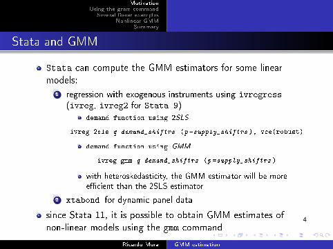
Stata and GMM

Stata can compute the GMM estimators for some linear models:

1 regression with exogenous instruments using ivregress (ivreg, ivreg2 for Stata 9)

demand function using 2SLS

ivreg 2sls q demand_shiftrs (p =supply_shiftrs ), vce(robust)

demand function using GMM

ivreg gmm q demand_shiftrs (p =supply_shiftrs )

with heteroskedasticity, the GMM estimator will be more

e°cient than the 2SLS estimator

2 xtabond for dynamic panel data

since Stata 11, it is possible to obtain GMM estimates of non-linear models using the gmm command


4



Summary



5



Summary


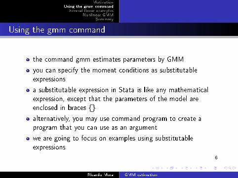
the command gmm estimates parameters by GMM

you can specify the moment conditions as substitutable expressions

a substitutable expression in Stata is like any mathematical expression, except that the parameters of the model are enclosed in braces {}

alternatively, you may use command program to create a program that you can use as an argument

we are going to focus on examples using substitutable expressions


6



Summary

The syntax of gmm with instruments

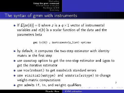
If E [ze(b)] = 0 where z is a q × 1 vector of instrumental variables and e(b) is a scalar function of the data and the parameters beta

gmm (e (b)) , instruments(z_list) options

by default, it computes the two-step estimator with identity matrix in the ˝rst step

use onestep option to get the one-step estimator and igmm to get the iterative estimator

use vce(robust) to get sandwich standard errors use winitial(wmtype) and wmatrix(witype) to change weight-matrix computations

gmm admits if, in, and weight quali˝ers


7



Summary

More general moment conditions (1)

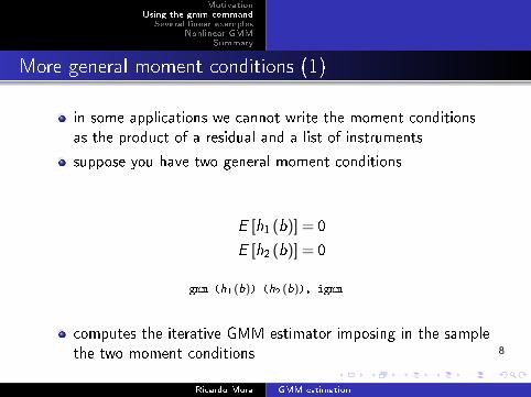
in some applications we cannot write the moment conditions as the product of a residual and a list of instruments

suppose you have two general moment conditions

E [h1 (b)] = 0

E [h2 (b)] = 0

gmm (h1 (b)) (h2 (b)), igmm

computes the iterative GMM estimator imposing in the sample the two moment conditions


8



Summary

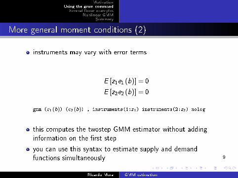
More general moment conditions (2)

instruments may vary with error terms

E [z1e1 (b)] = 0

E [z2e2 (b)] = 0

gmm (e1 (b)) (e2 (b)) , instruments(1:z1) instruments(2:z2) nolog

this computes the twostep GMM estimator without adding information on the ˝rst step

you can use this syntax to estimate supply and demand functions simultaneously


9



Summary

Several linear examples


10



Summary

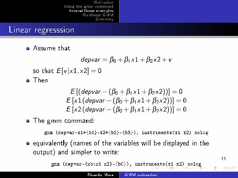
Linear regresssion

Assume that

depvar = β0 + β1x 1+ β2x 2+ v

so that E [v |x 1,x 2] = 0 Then

E [(depvar − (β0 + β1x 1+ β2x 2))] = 0 E [x 1(depvar − (β0 + β1x 1+ β2x 2))] = 0 E [x 2(depvar − (β0 + β1x 1+ β2x 2))] = 0

The gmm command:

gmm (depvar-x1*{b1}-x2*{b2}-{b3}), instruments(x1 x2) nolog

equivalently (names of the variables will be displayed in the output) and simpler to write:

gmm (depvar-{xb:x1 x2}-{b0}), instruments(x1 x2) nolog


11



Summary

Estimating OLS with gmm command

. regress mpg gear_ratio turn, r

Linear regression Number of obs = 74F( 2, 71) = 47.92Prob > F = 0.0000R-squared = 0.5483Root MSE = 3.9429

------------------------------------------------------------------------------| Robust

mpg | Coef. \Std. Err. t P>|t| [95% Conf. Interval]-------------+---------------------------------------------------------------- gear_ratio | 3.032884 1.533061 1.98 0.052 -.023954 6.089721

turn | -.7330502 .1204386 -6.09 0.000 -.9731979 -.4929025_cons | 41.21801 8.5723 4.81 0.000 24.12533 58.31069

------------------------------------------------------------------------------

gmm (mpg - {b1}*gear_ratio - {b2}*turn - {b0}), instruments(gear_ratio turn) nolog

Final G\M\M criterion Q(b) = 3.48e-32

G\M\M estimation

Number of parameters = 3Number of moments = 3Initial weight matrix: Unadjusted Number of obs = 74G\M\M weight matrix: Robust

------------------------------------------------------------------------------| Robust| Coef. \Std. Err. z P>|z| [95% Conf. Interval]

-------------+----------------------------------------------------------------/b1 | 3.032884 1.501664 2.02 0.043 .0896757 5.976092/b2 | -.7330502 .117972 -6.21 0.000 -.9642711 -.5018293/b0 | 41.21801 8.396739 4.91 0.000 24.76071 57.67532

------------------------------------------------------------------------------Instruments for equation 1: gear_ratio turn _cons


12



Summary

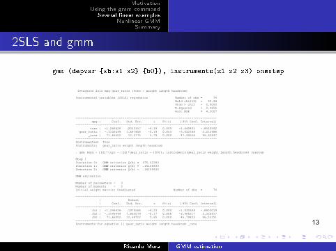
2SLS and gmm

gmm (depvar-{xb:x1 x2}-{b0}), instruments(z1 z2 z3) onestep

ivregress 2sls mpg gear_ratio (turn = weight length headroom)

Instrumental variables (2SLS) regression Number of obs = 74Wald chi2(2) = 90.94Prob > chi2 = 0.0000R-squared = 0.4656Root MSE = 4.2007

------------------------------------------------------------------------------mpg | Coef. Std. Err. z P>|z| [95% Conf. Interval]

-------------+----------------------------------------------------------------turn | -1.246426 .2012157 -6.19 0.000 -1.640801 -.8520502

gear_ratio | -.3146499 1.697806 -0.19 0.853 -3.642288 3.012988_cons | 71.66502 12.3775 5.79 0.000 47.40556 95.92447

------------------------------------------------------------------------------Instrumented: turnInstruments: gear_ratio weight length headroom

. gmm (mpg - {b1}*turn - {b2}*gear_ratio - {b0}), instruments(gear_ratio weight length headroom) onestep

\Step 1Iteration 0: G\M\M criterion Q(b) = 475.42283 Iteration 1: G\M\M criterion Q(b) = .16100633 Iteration 2: G\M\M criterion Q(b) = .16100633

G\M\M estimation

Number of parameters = 3Number of moments = 5Initial weight matrix: Unadjusted Number of obs = 74

------------------------------------------------------------------------------| Robust| Coef. Std. Err. z P>|z| [95% Conf. Interval]

-------------+----------------------------------------------------------------/b1 | -1.246426 .1970566 -6.33 0.000 -1.632649 -.8602019/b2 | -.3146499 1.863079 -0.17 0.866 -3.966217 3.336917/b0 | 71.66502 12.68722 5.65 0.000 46.79853 96.53151

------------------------------------------------------------------------------Instruments for equation 1: gear_ratio weight length headroom _cons


13



Summary

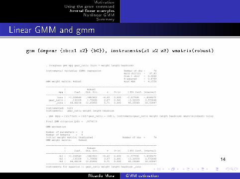
Linear GMM and gmm

gmm (depvar-{xb:x1 x2}-{b0}), instruments(z1 z2 z3) wmatrix(robust)

. ivregress gmm mpg gear_ratio (turn = weight length headroom)

Instrumental variables (GMM) regression Number of obs = 74 Wald chi2(2) = 97.83 Prob > chi2 = 0.0000 R-squared = 0.4769

GMM weight matrix: Robust Root MSE = 4.1559

------------------------------------------------------------------------------ | Robust

mpg | Coef. Std. Err. z P>|z| [95% Conf. Interval] -------------+----------------------------------------------------------------

turn | -1.208549 .1882903 -6.42 0.000 -1.577591 -.8395071 gear_ratio | .130328 1.75499 0.07 0.941 -3.30939 3.570046

_cons | 68.89218 12.05955 5.71 0.000 45.25589 92.52847 ------------------------------------------------------------------------------ Instrumented: turn Instruments: gear_ratio weight length headroom

. gmm (mpg - {b1}*turn - {b2}*gear_ratio - {b0}), instruments(gear_ratio weight length headroom) wmatrix(robust) nolog

Final G\M\M criterion Q(b) = .0074119

G\M\M estimation

Number of parameters = 3 Number of moments = 5 Initial weight matrix: Unadjusted Number of obs = 74 G\M\M weight matrix: Robust

------------------------------------------------------------------------------ | Robust | Coef. Std. Err. z P>|z| [95% Conf. Interval]

-------------+---------------------------------------------------------------- /b1 | -1.208549 .1882903 -6.42 0.000 -1.577591 -.8395071 /b2 | .130328 1.75499 0.07 0.941 -3.30939 3.570046 /b0 | 68.89218 12.05955 5.71 0.000 45.25589 92.52847

------------------------------------------------------------------------------ Instruments for equation 1: gear_ratio weight length headroom _cons


14



Summary

Nonlinear GMM


15



Summary

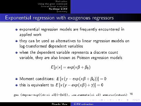
Exponential regression with exogenous regressors

exponential regression models are frequently encountered in applied work

they can be used as alternatives to linear regression models on log-transformed dependent variables

when the dependent variable represents a discrete count variable, they are also known as Poisson regression models

E [y |x ] = exp(x β + β0)

Moment conditions: E [x (y − exp (x β + β0))] = 0

this is equivalent to E [x (y − exp (x β )+ γ)] = 0

gmm (depvar-exp({xb:x1 x2})+{b0}), instruments(x1 x2) wmatrix(robust)


16



Summary

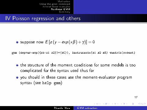
IV Poisson regression and others

suppose now E [z (y − exp (x β )+ γ)] = 0

gmm (depvar-exp({xb:x1 x2})+{b0}), instruments(z1 z2 z3) wmatrix(robust)

the structure of the moment conditions for some models is too complicated for the syntax used thus far

you should in these cases use the moment-evaluator program syntax (see help gmm)


17



Summary

Summary

Stata can compute the GMM estimators for some linear models:

1 regression with exogenous instruments using ivregress (ivreg, ivreg2 for Stata 9)

2 xtabond for dynamic panel data

since Stata 11, it is possible to obtain GMM estimates of non-linear models using the gmm command


18

MIT OpenCourseWare https://ocw.mit.edu

14.382 Econometrics Spring 2017

For information about citing these materials or our Terms of Use, visit: https://ocw.mit.edu/terms.

19

https://ocw.mit.edu/

https://ocw.mit.edu/terms

GMM Estimation in Stata - MIT OpenCourseWare · the command gmm estimates parameters by GMM you can...

Documents

Transcript of GMM Estimation in Stata - MIT OpenCourseWare · the command gmm estimates parameters by GMM you can...