GMDTF Framing - nerc.com Disturbance Task Force... · AEP – Kwin Que. BottlierMagnitometer ......

GMDTF Framing

Don Watkins, Bonneville Power Administration

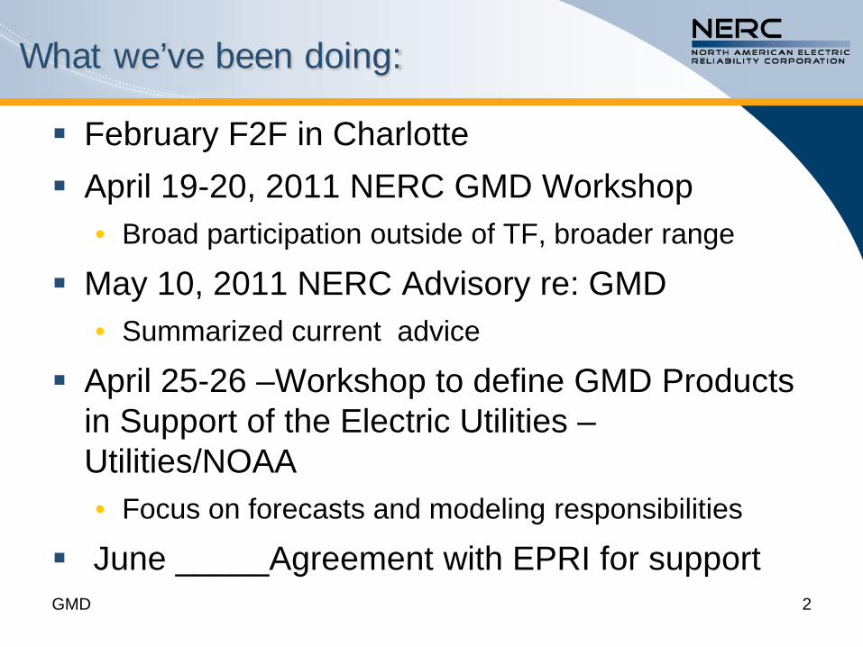
What we’ve been doing:

February F2F in Charlotte April 19-20, 2011 NERC GMD Workshop

• Broad participation outside of TF, broader range

May 10, 2011 NERC Advisory re: GMD• Summarized current advice

April 25-26 –Workshop to define GMD Products in Support of the Electric Utilities –Utilities/NOAA• Focus on forecasts and modeling responsibilities

June _____Agreement with EPRI for supportGMD 2

Mission/Makeup

The Geomagnetic Disturbance Task Force (GMDTF) will investigate bulk power system reliability implications of [GMD] risks and develop solutions to help mitigate this risk.

Our Task Force has nearly 80 people on its roster including equipment experts, utility engineers, Scientists, and government representatives.

Deliverables per Scope

2011 Deliverables

1st Quarter

Whitepaper outlining the current industry experience and capability and identifies opportunities, options and alternatives to enhanced how the industry manages GMD risks. [Activity: Assimilated regional plans, NERC GMD advisory

2nd QuarterWhitepaper on current warning limitations, the ability of operators to take mitigating action, and areas for improvement.

3rd Quarter Whitepaper on restoration abilities and areas for improvement.

4th Quarter(Dependencies)

1.Whitepaper that reviews industry prevention approaches to GMD events. 2.Final report incorporating the findings of the whitepapers and simulations with suggested recommendations and follow-on actions.

Where we are: Products – (all Draft)

NERC GMD Advisory

GMDTF-1 Compilation of Current GMD Reliability Coordinator Operating Procedures–March 2011 (internal)

Draft Subgroup 1 Whitepaper – Procedures & Equipment - May 2011

Draft Subgroup 2 Whitepaper – Modeling May 2011

GMD 5

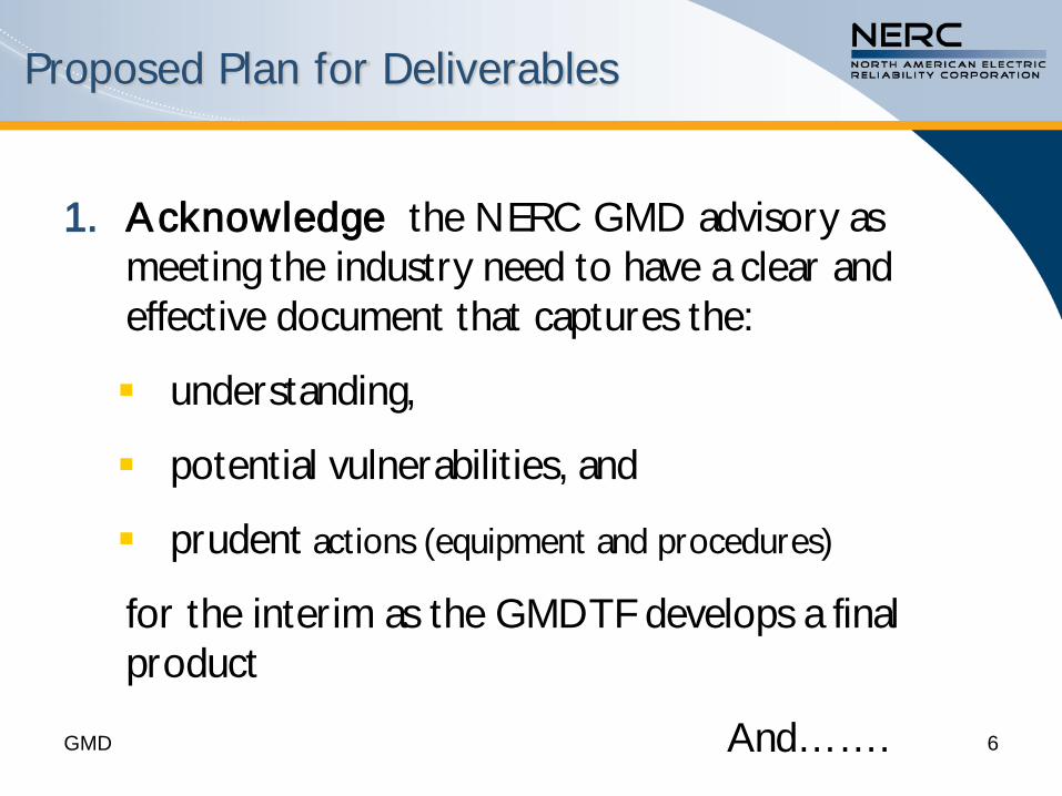
1. Acknowledge the NERC GMD advisory as meeting the industry need to have a clear and effective document that captures the:

understanding,

potential vulnerabilities, and

prudent actions (equipment and procedures)

for the interim as the GMDTF develops a final product

And…….

Proposed Plan for Deliverables

GMD 6


2. Focus our efforts on all the elements of our final product including:

Identifying the “chapters”

Develop the scientific and engineering approaches to each chapter.

Actively and formally vet all technical findings to the degree necessary.

Produce the a final product that is also publically vetted


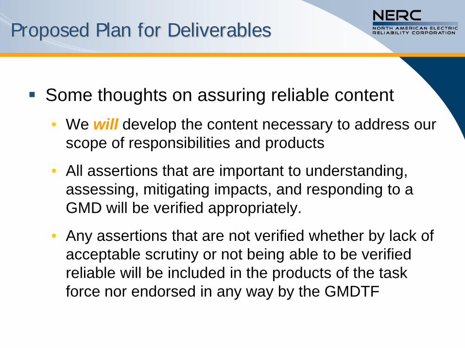
Some thoughts on assuring reliable content• We will develop the content necessary to address our

scope of responsibilities and products

• All assertions that are important to understanding, assessing, mitigating impacts, and responding to a GMD will be verified appropriately.

• Any assertions that are not verified whether by lack of acceptable scrutiny or not being able to be verified reliable will be included in the products of the task force nor endorsed in any way by the GMDTF

Critical Priorities (We must get this right!)

Transformer Vulnerability• ID vulnerability, prioritize, establish characteristics (GIC vs T)

• This is the primary reason for concern with GMD

• What is your “Live to fight the next day.” plan in an extreme storm?

“Reference Event” – given a locational 1:100y:How should we establish performance requirements? :

• Each system should be able to withstand the reference storm, or

• Should each do what is prudent in their own estimation

• Should it be a reference worse credible case with each entity deciding how to protect their system? (This is where we are headed)

(Did I mention that we have to get this right?)

GMDTF Deliverables – Final Report

GMD 10

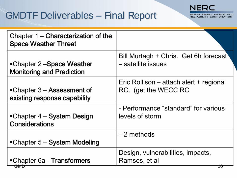
Chapter 1 – Characterization of the Space Weather Threat

Chapter 2 –Space Weather Monitoring and Prediction

Bill Murtagh + Chris. Get 6h forecast – satellite issues

Chapter 3 – Assessment of existing response capability

Eric Rollison – attach alert + regional RC. (get the WECC RC

Chapter 4 – System Design Considerations

- Performance “standard” for various levels of storm

Chapter 5 – System Modeling – 2 methods

Chapter 6a - TransformersDesign, vulnerabilities, impacts, Ramses, et al


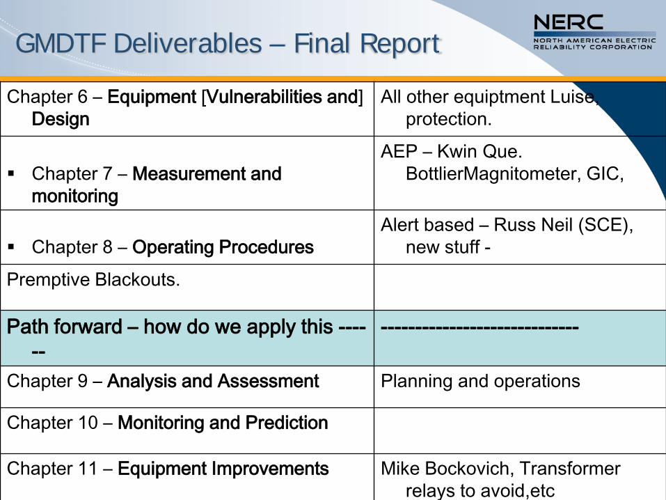
Chapter 6 – Equipment [Vulnerabilities and]Design

All other equiptment Luise, protection.

Chapter 7 – Measurement and monitoring

AEP – Kwin Que. BottlierMagnitometer, GIC,

Chapter 8 – Operating ProceduresAlert based – Russ Neil (SCE),

new stuff -Premptive Blackouts.

Path forward – how do we apply this ------

-----------------------------

Chapter 9 – Analysis and Assessment Planning and operations

Chapter 10 – Monitoring and Prediction

Chapter 11 – Equipment Improvements Mike Bockovich, Transformer relays to avoid,etc


What is missing? Changes? (e.g.): • “Reference Storm

• Guidelines or performance requirements

Will this serve our “customers”?

Specific issues we will need to address beyond the Science and engineering?

GMD 12

GMDTF Deliverables – Final Report Proposed Time line

Topic/Issue related workshops? Methodology?

US and Canadian Govmt Workshops?

August 30th ?? for External review (2 wk before Committees)

Further refinement

December 29th – Submittal for Approval by NERC Technical Committees

Pulkkinen, A.1, J. Eichner2 and others to by included to the author

list1 CUA and NASA/GSFC Community Coordinated

Modeling Center, Greenbelt, USA.2Munich-Re, Munich, Germany.

Generation of 100-year geomagnetically induced

current scenarios

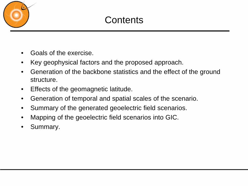
Contents

• Goals of the exercise.• Key geophysical factors and the proposed approach.• Generation of the backbone statistics and the effect of the ground

structure.• Effects of the geomagnetic latitude.• Generation of temporal and spatial scales of the scenario.• Summary of the generated geoelectric field scenarios.• Mapping of the geoelectric field scenarios into GIC.• Summary.

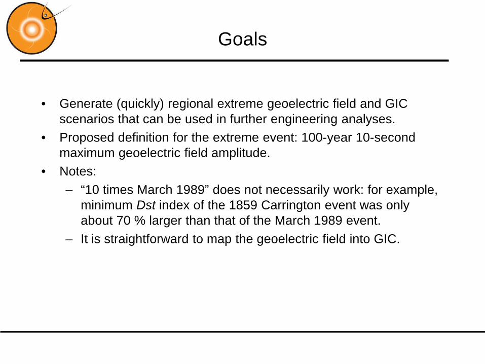
Goals

• Generate (quickly) regional extreme geoelectric field and GIC scenarios that can be used in further engineering analyses.

• Proposed definition for the extreme event: 100-year 10-second maximum geoelectric field amplitude.

• Notes:– “10 times March 1989” does not necessarily work: for example,

minimum Dst index of the 1859 Carrington event was only about 70 % larger than that of the March 1989 event.

– It is straightforward to map the geoelectric field into GIC.

Four key geophysical factors that need to be addressed

• The effect of the ground conductivity structure on the extreme geoelectric field amplitudes.

• The effect of the geomagnetic latitude on the extreme geoelectric field amplitudes.

• Temporal scales of the extreme events.• Spatial scales of the extreme events.

Four key geophysical factors that need to be addressed

• The effect of the ground conductivity structure on the extreme geoelectric field amplitudes - two ground conductivity models representing realistic extreme ends of conducting and resistive grounds are applied.

• The effect of the geomagnetic latitude on the extreme geoelectric field amplitudes - we will identify a threshold geomagnetic latitude across which the maximum geoelectric field amplitudes experience approximately an order of magnitude decrease.

• Temporal scales of the extreme events - representative time series from selected magnetometer stations for a major event storm event are used to provide realistic temporal profiles.

• Spatial scales of the extreme events - we will assume uniform geoelectric field structure in regional scales. Generating a global scenario will be significantly more complicated due to poorly known spatiotemporal geoelectric field correlations at global scales.

Selected approach

1) Assume regionally (100-1000 km) spatially uniform geoelectric field. Assumption may not always hold especially at high-latitude locations.

2) Select a storm event and super- and sub-threshold geomagnetic observatories to obtain representative temporal storm profiles. Compute the geoelectric field and normalize the amplitudes.

3) Scale the normalized geoelectric field amplitudes obtained via 2) to obtain 100-year 10-second maximum amplitude event. Use previously computed statistics to determine the maximum amplitudes (Pulkkinen et al., 2008).

4) Compute GIC. Direct linear mapping or quasi-dc power grid model can be utilized.

Generation of the statistics and the effect of the ground conductivity

Statistical occurrence of modeled geoelectric field in Quebec and British Columbia (Pulkkinen et al., 2008)

Visual extrapolation to 100-year amplitudes

Quebec modelBritish Columbia model

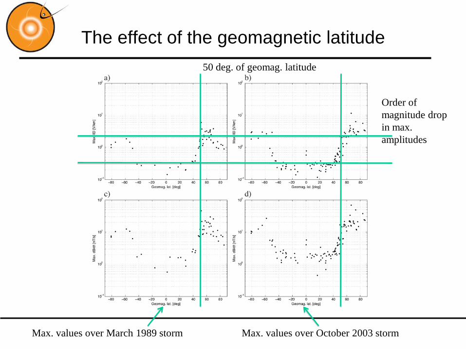
The effect of the geomagnetic latitude

Max. values over March 1989 storm Max. values over October 2003 storm

Order of magnitude drop in max. amplitudes

50 deg. of geomag. latitude

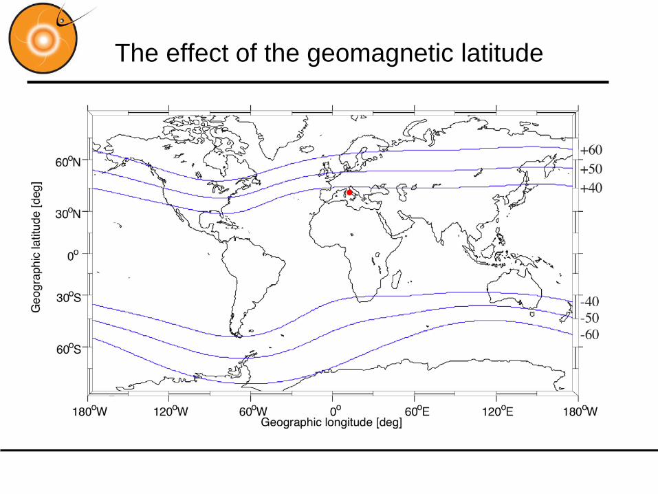
The effect of the geomagnetic latitude

Temporal scales

• Need to capture great variety of geospace processes and temporal scales associated with extreme storms. Chose to use observational data for a major event to capture the variability.

• We use two representative stations. One from sub-threshold latitudes (Memanbetsu, Japan, 37 deg. of geomagnetic latitude) and another one from super-threshold latitudes (Nurmijärvi, Finland, 57 deg. of geomagnetic latitude).

• 10-s geomagnetic field observations from the two stations for 29-31, October 2003 provide representation of the temporal profiles.

• Geomagnetic field mapped into geoelectric field using the plane wave method and the Quebec ground model. Amplitudes normalized for scaling.

Temporal scales (normalized fields)

Spatial scales

• Two-fold nature of major and extreme events: a) large geoelectric field magnitudes can be experienced across the globe in the region covered by the auroral current system, b) spatial correlation lengths associated with the field fluctuations can be short.

• Spatial GIC and geoelectric field correlations on global scale not well-known.

• We will assume spatially uniform geoelectric field on regional (100-1000 km ) scales.

Summary of the scenarios

Mapping to GIC

• Apply extreme geoelectric field scenarios to quasi-dc models of the regional grid obtain GIC through each node of the system.

• Or apply simply (shown to hold to a good approximation):GIC(t) = aEx(t) + bEy(t)System parameters

Geoelectric field scenario

Summary

• Extreme regional geoelectric field scenarios generated as a function of ground conductivity structure and geomagnetic latitude.

• Numerical data for scenarios publicly available for mapping to GIC and further engineering analyses. Note: further refinements to the scenarios likely.

• For details, see Pulkkinen et al., 2011 (draft of the manuscript prepared).

EPRI / NERC Statement of Work

Geomagnetic Disturbance

2© 2011 Electric Power Research Institute, Inc. All rights reserved.

Education

Research Question• State of the knowledge on GMDs• How to effectively convey to decision

makers • What magnitudes of currents occurEPRI Strategy :• Interest Group• Summarize Past Work• Measure Induced Currents (Sunburst)Status:• White paper completed• Interest Group being formed• Sunburst Network being expanded


Vulnerability Assessment

Research Question• Impacts to grid • Determine influencing factorsEPRI Strategy:• Measure induced currents (Sunburst)• Assessing vulnerability of

Transformers• System wide modelingStatus:- Sunburst Network Being Expanded- 6 Transformer Assessments ongoing- Scoping System Models


Mitigation

Research Questions• Warnings & procedures for operators• Effectively blocking of GICs • Relay trip transformers EPRI Strategy :• Laboratory testing of blockers • R&D on relay parameters• Collaborate with NASA on Solar Shield

utilizing SunburstStatus:• Launch Supplemental on Testing & Relay

parameters• Support NASA


Deep Dive on Today’s Discussion – Task 2 Vulnerability Assessment

• Detailed system modeling will be performed in three regions (TBD) of the EHV grid to assess its vulnerability to GMD.

• Particular emphasis will be placed on:

– Possible effects of GIC on large power transformers

– Increased var consumption → voltage stability

– Harmonic generation and related effects on equipment such as capacitor banks, harmonic filters, etc.

– GIC effects on protection and control (P&C) systems


Modeling and Analysis Approach

• Task 2A - Determine GIC flows in network using available data and assumptions.

• Task 2B - Perform AC load flow with additional var demand caused by ½ cycle saturation.

• Task 2C - Perform time-domain analysis to determine possible harmonic generation due to ½ cycle saturation, and potential impacts on power quality and equipment such as capacitor banks, harmonic filters and transformers.

• Task 2D -Using information from time-domain analysis in Task 2C, determine potential impacts on system protection and control (P&C).

• Task 2E - Screen vulnerable transformers to more manageable list.


Task 2A - GIC Flow Analysis

• An open source software program will be developed to determine GIC flows in the transmission grid.– Capable of performing multiple cases (contingency

analysis)

OpenGIC

dB/dtPSS/EPSLFCAPE

ASPEN

System Data

σ

Sub & LineLocation Data

GIC flows

E

∆Mag Field/∆time

Earth Cond.

Earth Surface Potential

Electric Field Gradient (V/m)


Task 2B – AC Load Flow Analysis

• When a transformer begins to saturate due to GIC, its reactive power demand increases dramatically.

• This effect must be taken into account in an AC load flow analysis to ensure that system voltage is not depressed beyond limits.

QSystemSystem

dckIQ ≈ Additional var demand dueto half cycle saturation


Task 2C – Time-Domain Analysis

• Time-domain simulations will be performed using EMTP-RV to analyze impacts of GIC in more detail.– Requires more sophisticated system model than GIC

flow or AC load flow analysis

EMTP-RV

GIC FlowsPSS/EPSLFCAPE

ASPEN

System Data

Sat. Curves

Harmonics

Waveforms

FFT

COMTRADE


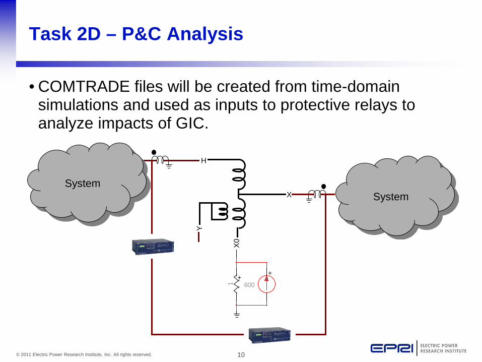
Task 2D – P&C Analysis

• COMTRADE files will be created from time-domain simulations and used as inputs to protective relays to analyze impacts of GIC.

H

XY

X0

+

600

+1

SystemSystem


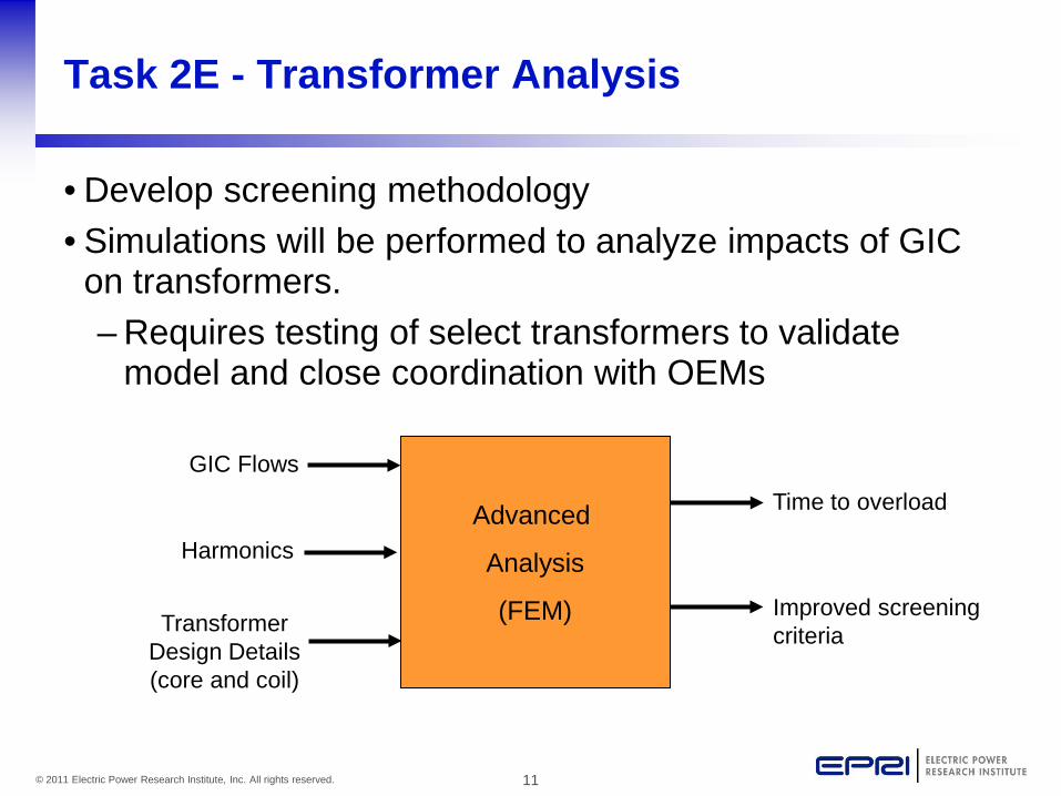
Task 2E - Transformer Analysis

• Develop screening methodology• Simulations will be performed to analyze impacts of GIC

on transformers.– Requires testing of select transformers to validate

model and close coordination with OEMs

Advanced

Analysis

(FEM)

GIC Flows

TransformerDesign Details(core and coil)

Harmonics

Time to overload

Improved screening criteria


Together…Shaping the Future of Electricity

1

AN ANALYSIS OF THE THREAT POTENTIAL TO THE US ELECTRIC POWER GRID FROM

SEVERE GEOMAGNETIC STORMS Storm-R-111

Storm AnalysisConsultants

John G. Kappenman, P.E.Principal Consultant

Voice: (218) 727-2666Fax: (218) 727-2728E-Mail: [email protected]

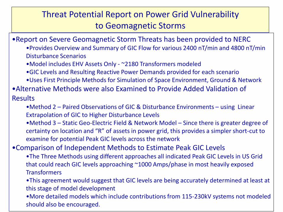
Threat Potential Report on Power Grid Vulnerability to Geomagnetic Storms

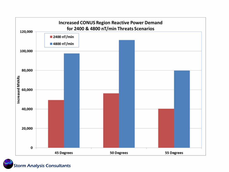
•Report on Severe Geomagnetic Storm Threats has been provided to NERC•Provides Overview and Summary of GIC Flow for various 2400 nT/min and 4800 nT/min Disturbance Scenarios •Model includes EHV Assets Only - ~2180 Transformers modeled•GIC Levels and Resulting Reactive Power Demands provided for each scenario•Uses First Principle Methods for Simulation of Space Environment, Ground & Network

•Alternative Methods were also Examined to Provide Added Validation of Results

•Method 2 – Paired Observations of GIC & Disturbance Environments – using Linear Extrapolation of GIC to Higher Disturbance Levels•Method 3 – Static Geo-Electric Field & Network Model – Since there is greater degree of certainty on location and “R” of assets in power grid, this provides a simpler short-cut to examine for potential Peak GIC levels across the network

•Comparison of Independent Methods to Estimate Peak GIC Levels•The Three Methods using different approaches all indicated Peak GIC Levels in US Grid that could reach GIC levels approaching ~1000 Amps/phase in most heavily exposed Transformers•This agreement would suggest that GIC levels are being accurately determined at least at this stage of model development•More detailed models which include contributions from 115-230kV systems not modeled should also be encouraged.

Space Environment Model Complex Temporal & Spatial Dynamics

Modeling Space Weather to Power Grid Performance

•Process Requires development and linkage of four dynamic and complex modeling domains•The greatest uncertainty arises in the Ground Model and AC Behavior Models•Many steps taken to benchmark each model separately and in unison•Performance of model generally produces conservative threat estimates

Layered-Earth Ground ModelGeospatial Complexity & Frequency Response

Power Grid GIC Model – Complex topology & circuit apparatus for GIC Flows

-750

-500

-250

0

250

500

750

1000

1250

1500

0.00 16.67 33.33 50.00 66.67 83.33 100.00 116.67

Time (msec)

Tran

sfor

mer

500

kV W

indi

ng C

urre

nt (A

mps

)

Current with GIC SaturationNormal Current

Grid AC Performance Model – estimates grid stress

Benchmark RegionRockport & Marysyille

Benchmark RegionForbes

Benchmark Region

Bell, Monroe

Benchmark Region

Moss Landing

Storm is relatively weak – lack of coherent magnetic field disturbance presents challenging environment to model

Benchmarking the US Grid Model – Feb 21, 1994 Storm

Benchmark RegionHope Creek & PLV

Benchmark RegionChester

Storm Analysis Consultants

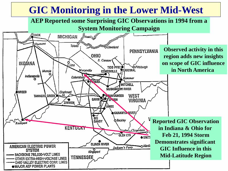
AEP Reported some Surprising GIC Observations in 1994 from aSystem Monitoring Campaign

Observed activity in thisregion adds new insights

on scope of GIC influencein North America

Reported GIC Observationin Indiana & Ohio for

Feb 21, 1994 StormDemonstrates significant

GIC Influence in thisMid-Latitude Region

GIC Monitoring in the Lower Mid-West

13:35UT Feb 21, 1994 14:04UT Feb 21, 1994

Geomagnetic Storm Environment Specification


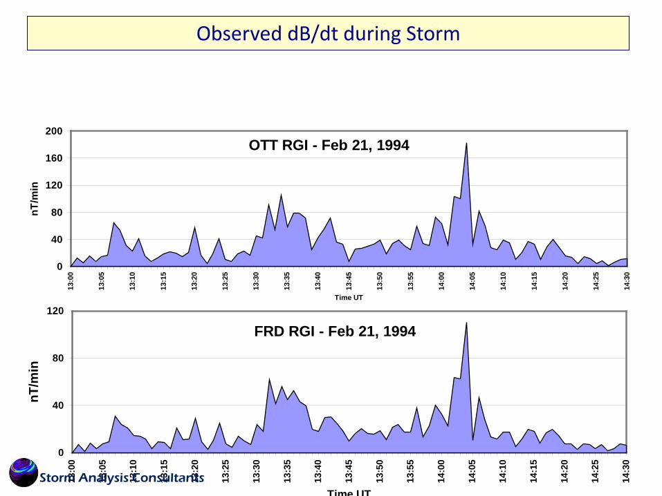
FRD RGI - Feb 21, 1994

0

40

80

120

13:0

0

13:0

5

13:1

0

13:1

5

13:2

0

13:2

5

13:3

0

13:3

5

13:4

0

13:4

5

13:5

0

13:5

5

14:0

0

14:0

5

14:1

0

14:1

5

14:2

0

14:2

5

14:3

0

Time UT

nT/m

in

OTT RGI - Feb 21, 1994

0

40

80

120

160

200

13:0

0

13:0

5

13:1

0

13:1

5

13:2

0

13:2

5

13:3

0

13:3

5

13:4

0

13:4

5

13:5

0

13:5

5

14:0

0

14:0

5

14:1

0

14:1

5

14:2

0

14:2

5

14:3

0

Time UT

nT/m

inObserved dB/dt during Storm


Simulated Rockport T1 Neutral GIC - Feb 21, 1994

-20

-10

0

10

20

30

13:00

13:05

13:10

13:15

13:20

13:25

13:30

13:35

13:40

13:45

13:50

13:55

14:00

14:05

14:10

14:15

14:20

14:25

14:30

Time UT

Neutr

al GI

C (A

mps)

Observed GIC

Simulated GIC

GIC Observations/Simulations in the Lower Mid-West

Marysville Simulated Neutral GIC - Feb 21, 1994

-6

-4

-2

0

2

4

6

8

13:00 13:15 13:30 13:45 14:00 14:15 14:30

Time UT

Am

ps

Observed GIC

Simulated GIC

GIC Observations/Simulations in the Lower Mid-West


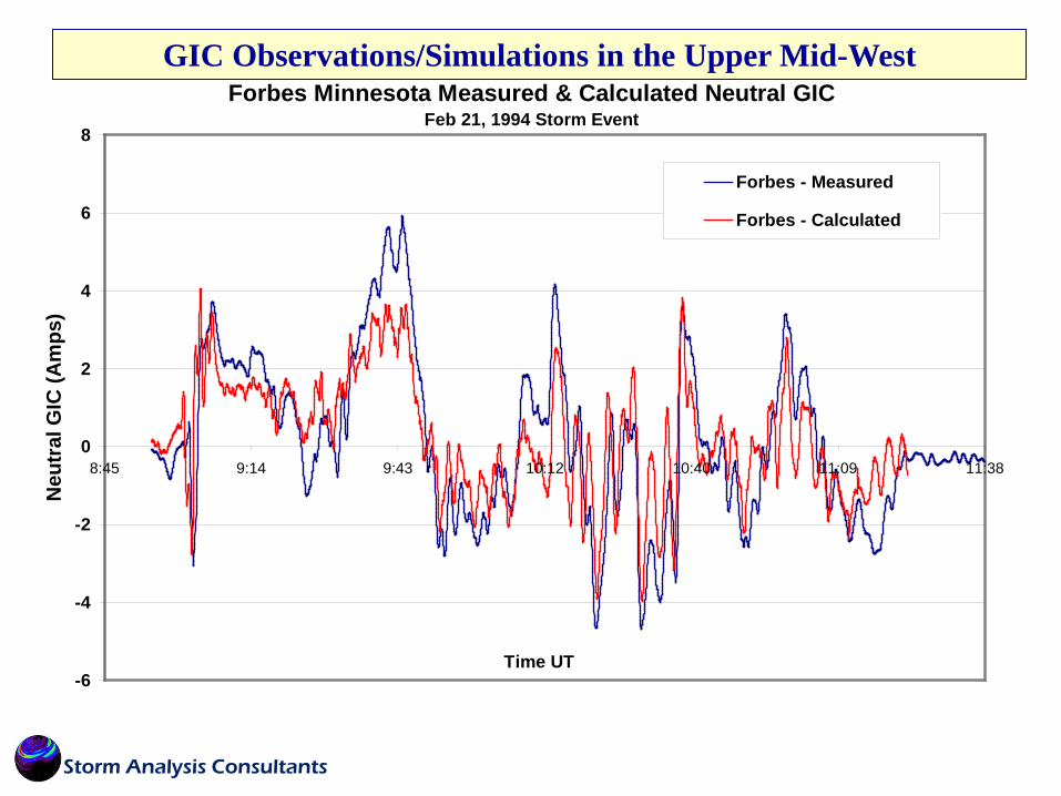
Forbes Minnesota Measured & Calculated Neutral GICFeb 21, 1994 Storm Event

-6

-4

-2

0

2

4

6

8

8:45 9:14 9:43 10:12 10:40 11:09 11:38

Time UT

Neu

tral

GIC

(Am

ps)

Forbes - Measured

Forbes - Calculated

GIC Observations/Simulations in the Upper Mid-West


Comparison of Observed and Calculated Peak GICFeb 21-22, 1994 Storm Event

0

5

10

15

20

25

30

35

40

45

Bell Chester CPS Hope Ck Marysvl Monroe Moss Ld PLV Rockpt SPA

Location

Neu

tral

GIC

(Am

ps)

Observed Peak GIC

Calculated Peak GIC

GIC Observations/Simulations Across the US


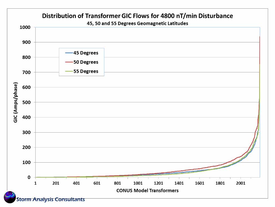
55o Threat Location

50o Threat Location

45o Threat Location

Based upon observations and expected storm dynamics a number of simulation scenarios have been developed to review potential threat extremes to the US Power Grid•2400 nT/min and 4800 nT/min Disturbances across the US (the 2400nT/min is likely a 1 in ~30 Year Scenario)•The most severe parts of the disturbances confined to a 5o wide Latitude Band (conservative estimate)•Various Equatorward Expansion Locations for these intense disturbances

Centered on 55o, 50o, and 45o Geo-Magnetic Latitude across North America

Overview for 4880 nT/min and 2400 nT/min Threat Scenario Simulations


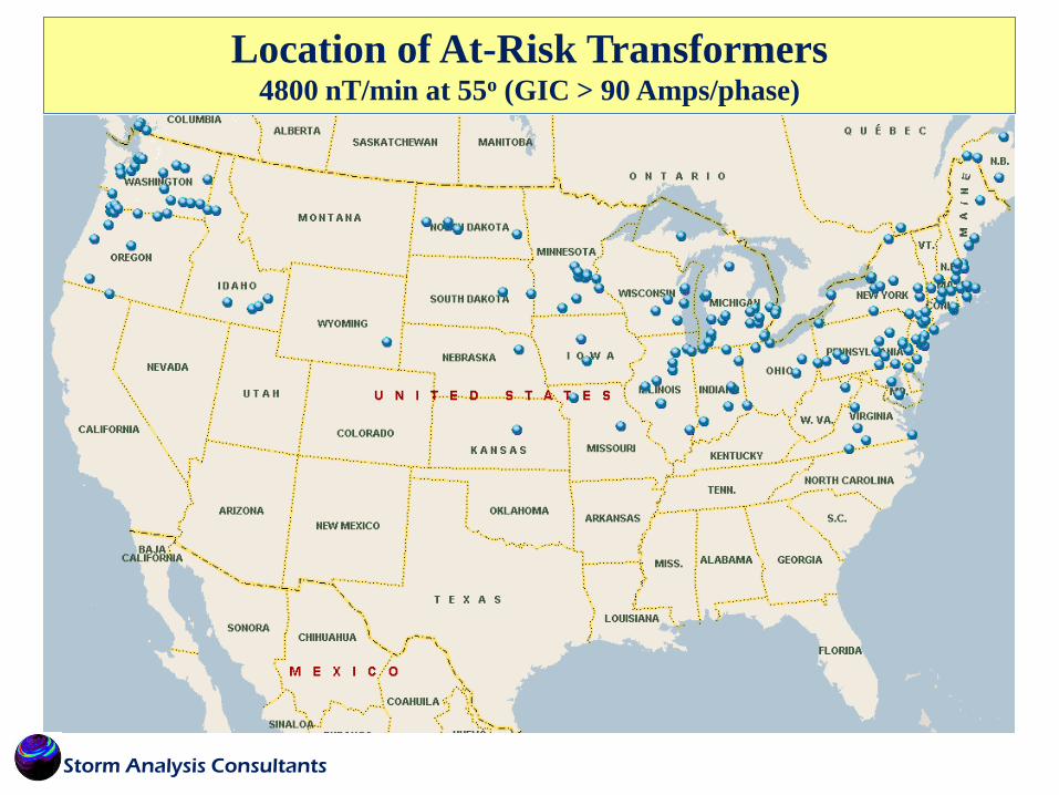
Location of At-Risk Transformers4800 nT/min at 55o (GIC > 90 Amps/phase)


Method 2 – Empirical Estimates of Peak GIC

•Paired Observations of GIC and Nearby Geomagnetic Observatory•Establish through observations at GIC and dB/dt that was driver of GIC at Network Location•Higher Storm dB/dt will also result in higher GIC (assuming all other factors are unchanged)•Valid to Assume Deep Earth Conductivity will not change or be influenced by saturation•Assume that Frequency Spectrum of Disturbance Environment is same •Assume Network Topology has no-change•For Auto-transformers we assume GIC in Neutral reflects 1/3 GIC per phase(??)•Orientation of threat environment unchanged•Linear Extrapolation to Estimate GIC

(GIC observed) /(dB/dt observed) = (GIC Estimated) / (dB/dt @ 4800 nT/min)

• Approach is very simple & straight forward• Takes into consideration all the important In-Situ factors that created Observed GIC • Limitation in that Only a Few Locations available for evaluation


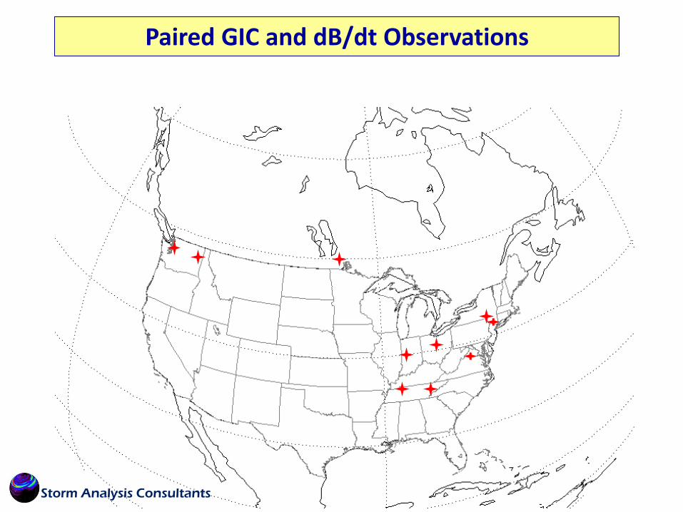
Paired GIC and dB/dt Observations


Mid-Atlantic

NY/NE/Can

South East

Defining Regions to Classify Region Specific Geomagnetic Storm Climatology

RGI for Mid-Atlantic Region – based on FRD Magnetic Observatory

RGI for Mid-Atlantic Region – based on BSL Magnetic Observatory

RGI for Mid-Atlantic Region – based on OTT Magnetic Observatory


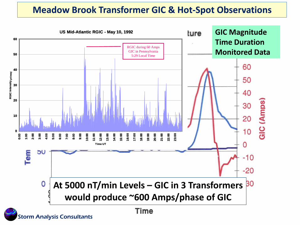
Meadow Brook Transformer GIC & Hot-Spot Observations

GIC MagnitudeTime DurationMonitored Data

US Mid-Atlantic RGIC - May 10, 1992

0

10

20

30

40

50

60

0:00

1:00

2:00

3:00

4:00

5:00

6:00

7:00

8:00

9:00

10:0

0

11:0

0

12:0

0

13:0

0

14:0

0

15:0

0

16:0

0

17:0

0

18:0

0

19:0

0

20:0

0

21:0

0

22:0

0

23:0

0

Time UT

RG

IC In

tens

ity

(nT/

min

)

RGIC during 60 Amps GIC in Pennsylvania

5:29 Local Time

US Mid-Atlantic RGIC - May 10, 1992

0

10

20

30

40

50

60

0:00

1:00

2:00

3:00

4:00

5:00

6:00

7:00

8:00

9:00

10:0

0

11:0

0

12:0

0

13:0

0

14:0

0

15:0

0

16:0

0

17:0

0

18:0

0

19:0

0

20:0

0

21:0

0

22:0

0

23:0

0

Time UT

RG

IC In

tens

ity

(nT/

min

)

RGIC during 60 Amps GIC in Pennsylvania

5:29 Local Time

At 5000 nT/min Levels – GIC in 3 Transformers would produce ~600 Amps/phase of GIC


NY Region RGIC Index - November 6, 2001

0

50

100

150

200

0:00

1:00

2:00

3:00

4:00

5:00

6:00

7:00

8:00

9:00

10:00

11:00

12:00

13:00

14:00

15:00

16:00

17:00

18:00

19:00

20:00

21:00

22:00

23:00

Time UT

nT/mi

nNov 6, 2001 Storm and GIC Measurements at Hurley Ave (NY)

60 Amps at 2:13EST Nov 24 (7:13 UT Nov 24)

7:13 UT


At 5000 nT/min Levels –would produce ~530 Amps/phase of GIC

119 nT/min @00:23UT

Oct 31, 2003

Oct 30-31, 2001 Storm and GIC Measurements in NY Region

At 5000 nT/min Levels – would produce ~1400 Amps/phase of GIC


Oct 28, 1991 Storm and GIC Measurements at South Canton (OH)

FRD RGI - Oct 28, 1991

0

50

100

150

200

250

0:00

1:00

2:00

3:00

4:00

5:00

6:00

7:00

8:00

9:00

10:0

0

11:0

0

12:0

0

13:0

0

14:0

0

15:0

0

16:0

0

17:0

0

18:0

0

19:0

0

20:0

0

21:0

0

22:0

0

23:0

0

Time UT

nT/m

in



Feb 21, 1994 Storm and GIC Measurements at Rockport (IN)

FRD RGI - Feb 21, 1994

0

40

80

120

13:0

0

13:0

5

13:1

0

13:1

5

13:2

0

13:2

5

13:3

0

13:3

5

13:4

0

13:4

5

13:5

0

13:5

5

14:0

0

14:0

5

14:1

0

14:1

5

14:2

0

14:2

5

14:3

0

Time UT

nT

/min



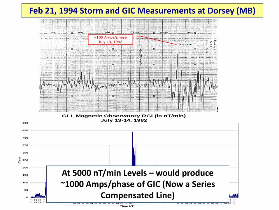
+105 Amps/phaseJuly 13, 1982

Feb 21, 1994 Storm and GIC Measurements at Dorsey (MB)

0

50

100

150

200

250

300

350

400

450

500

0:00

1:00

2:00

3:00

4:00

5:00

6:00

7:00

8:00

9:00

10:00

11:00

12:00

13:00

14:00

15:00

16:00

17:00

18:00

19:00

20:00

21:00

22:00

23:00 0:0

01:0

02:0

03:0

04:0

05:0

06:0

07:0

08:0

09:0

010

:0011

:0012

:0013

:0014

:0015

:0016

:0017

:0018

:0019

:0020

:0021

:0022

:0023

:00

nT/m

in

Time UT

GLL Magnetic Observatory RGI (in nT/min)July 13-14, 1982

At 5000 nT/min Levels – would produce ~1000 Amps/phase of GIC (Now a Series

Compensated Line)

-15

-10

-5

0

5

10

15

5 11 17 22 1 4 7 10 13 16 19 22 1 4 7 10 13 16 19 22 1 4

GIC

(Am

ps)

Time UT

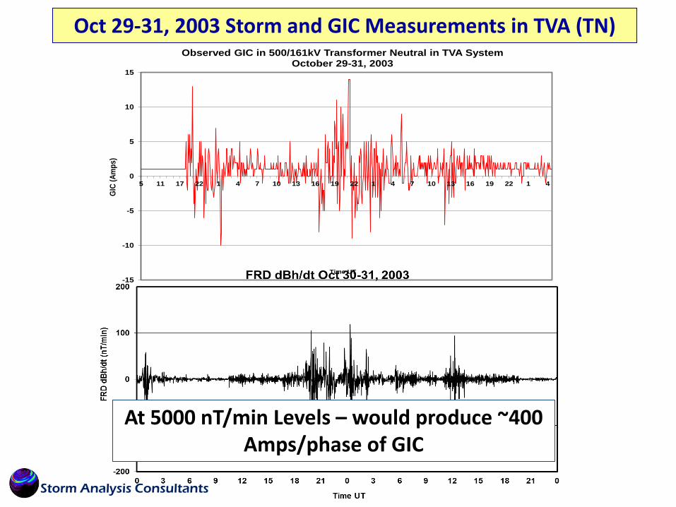
Observed GIC in 500/161kV Transformer Neutral in TVA System October 29-31, 2003

Oct 29-31, 2003 Storm and GIC Measurements in TVA (TN)



Oct 29-31, 2003 Storm and GIC Measurements at Bell BPA (WA)



Method 3 – Static Geo-Electric Field

•Limited Observations of Geo-Electric Field have been captured from Several Storms

•Using this Geo-Electric Field Data Directly, GIC Flow can be calculated•No Need for Storm Environment Model or Deep-Earth Conductivity Model•Model of Power Grid is all that is needed – have good confidence on Asset Locations and “R” of Lines and Transformers•Model Problem simplifies to Ohm’s Law and Geometry Calculations •Uncertainty Remains on How High can Peak Geo-Electric Field Reach


Uniform Geo-Electric Field – 0o (North)


Uniform Geo-Electric Field – 30o


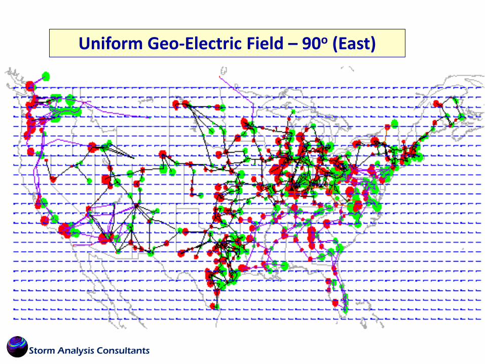
Uniform Geo-Electric Field – 90o (East)


7 V/km August 4, 1972

11 V/km July 16, 1892

~3V/km March 24, 1940

5.7 V/km Feb 19, 1852

Historically Observed Geo-Electric Fields

Note – 20 V/km has been measured in Europe during May 1921 Storm


Top 500 GIC Participation Transformers

Other Geomagnetic Storm Events can cause Large Geo-Electric Fields at Low Latitude Locations

Comparison of Electrojet-Driven and SSC Bx DisturbancesGLL Bx - March 13, 1989 and MSR Bx - March 24, 1991

-500

0

500

1000

1500

2000

2500

0:00 0:05 0:10 0:15 0:20 0:25 0:30 0:35 0:40 0:45 0:50

Time (min)

nT

MSR-BxGLL-Bx

Large Geo-Electric Fields & GICs at Low Latitude Locations

SSC Disturbance is Small but Fast and has Big Footprint

Electrojet Disturbance is Large but Slower than SSC


Comparison of Electrojet-Driven and SSC-Caused Geo-Electric FieldsGLL Bx - March 13, 1989 and MSR Bx - March 24, 1991

-4

-2

0

2

4

6

8

10

0:00 0:05 0:10 0:15 0:20 0:25 0:30 0:35 0:40 0:45 0:50

Time (min)

V/km

E-MSRE-GLL

Large Geo-Electric Fields & GICs at Low Latitude Locations

Small but Fast Geomagnetic Disturbance Produces Equivalently

Large GIC compared to Slower/Larger Disturbances


1E-5 1E-4 1E-3 0.01 0.11E-5

1E-4

1E-3

0.01

0.1

Spectral Response of Layered-Earth Ground Models

AOC1 ENG5 JNC6 SOO1 FOL3 NOS1 SOS2 NOR1 QNA1 BCA2 NNA3 NNA4 NNA5 CNA6 CNA7 CNA8

V/km

per

nT

Frequency (Hz)

SSC Bandwidth

EJ Bandwidth

SSC Content yields large Geo-Electric Field

Than Larger EJ Field of Low Frequency Content

Electrojet Intensification and SSC


GIC and Transformer Failure in New Zealand due to SSC

•Sudden Onset of Impulsive Geomagnetic Field Disturbance on Nov 6, 2001

•Transformer Located Hydro Station on South Island

•Failed within One Minute of Onset (1:52UT), Sudden Impulse Relay due to major internal flashover

This GIC Event is Identical in Timeframe to E3, but much smaller in magnitude

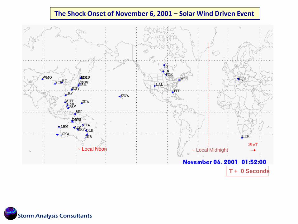
~ Local Noon ~ Local Midnight

T + 0 Seconds

The Shock Onset of November 6, 2001 – Solar Wind Driven Event


~ Local Midnight~ Local Noon

T + 8 Seconds

Just after SSC Onset, all Australian Observatories are first to observe

delta B changes



~ Local Midnight

T + 17 Seconds

Several Seconds later the delta B changes are clearly evident in

northern Hemisphere Asia.

~ Local Noon



~ Local Midnight

T + 49 SecondsDelta B changes are now beginning to appear

in night time regions of North America and Western Europe/South Africa

~ Local Noon



Observed GICs in Central Japan Power Grid - Nov 6, 2001

-50

-40

-30

-20

-10

0

10

20

30

40

50

1:00 1:30 2:00 2:30 3:00 3:30 4:00 4:30 5:00 5:30 6:00 6:30 7:00 7:30

Time UTG

IC (A

mps

)

GIC(A) SUNEN S/SGIC(A) SHINANO S/SGIC(A) FUKUMITSU BTB

Observed & Calculated GIC – Nov 6, 2001Southern/Central Japan

Meso-Scale Models Validation Across the System

Geo-Electric Field

GIC flows out of Network

GIC flows into Network


WORKSHOP TO DEFINE GEOMAGNETICSTORM PRODUCTS IN SUPPORT OF

THE ELECTRIC UTILITIES – THE WAYAHEAD

WORKSHOP TODEFINE GEOMAGNETIC STORM PRODUCTS INSUPPORT OF THE ELECTRIC UTILITIES – WAY AHEAD

• SWPC will work with partners for development continent-wide products depicting estimated electric field strength and direction. This will require a partnership with USGS, CCMC, NRCan, academia, private sector, and others.

• Validation and Verification is critical• Product must translate into “actionable” response

• SWPC and partners will investigate (currently working) ways to add more real-time ground magnetometer stations and to model ground conductivity.

It is likely that forecasts of dB/dt and the electric field will be very difficult.

• Therefore, forecasts of Kp, K, or alternate summary measures will be necessary for the near-term. It is possible to provide climatology for dB/dt, range, standard deviation, local electric field, for a given activity level. SWPC will work with partners to carry out this analysis and make such climatology tables available.

• SWPC will coordinate with the NERC and GMDTF personnel on an option for a teleconference with the NERC Reliability Coordinators in the event of an exceptional space weather situation (e.g., Oct 28-29 2003). Thresholds, quantitative measures, and response procedures need to be addressed.

When this would have happened – Oct 2003

When it may not have happened – Mar 1989

• SWPC will explore partnering with international partners, particularly NRCanada and the British Geological Survey (BGS), on the development and improvement of geomagnetic storm products and services.

• UK – US Agreement • Ongoing NR Canada efforts (International Space

Environment Service)

• Implement process for information sharing during and after geomagnetic disturbances. Feedback on system effects and impacts due to geomagnetic disturbances would be very valuable to space weather community for warning validation, and validation and verification of models.

• SWPC and partners will investigate alternate measures to local K-indices. The goal will be to have summary measures that extend the disturbance scale up to larger values to avoid saturation, and to have summary measures that can be compared in a meaningful way. Examples include, range, standard deviation, delta-B, and so on, all which are quantities that would be expressed in standard units (nT).

• SWPC and partners will also investigate a ‘storm catalog’ and will study better ways to characterize the envelope of these disturbances. This effort will address the requirement to characterize the intensity and duration of the disturbances.

• Solar wind measurements at L1 orbit are critical for space weather services

• Coronagraph vital for long-range (20-90 hrs)Currently provided by SOHO spacecraft - launched in 1996. STEREO

spacecraft of some value now but not for long!

• Critical model input

• Drives more accurate warnings

Currently provided by ACE spacecraft - launched in 1997.

Efforts to ensure follow-on, operationally dedicated missions need help.• Recommend GMDTF and community support

WATCH: Geomagnetic A-index of 50 or greater predictedIssue Time: 2001 Sep 24 1732 UTCValid for UTC Day: 2001 Sep 26NOAA Scale: Periods reaching the G3 (Strong) Level Likely

WARNING: Geomagnetic K-index of 7 or greater expectedValid From: 2001 Sep 06 1630 UTCValid To: 2001 Sep 07 2300 UTCWarning Condition: OnsetNOAA Scale: G3 or greater - Strong to Extreme

CME impacts ACE spacecraft

Prepared by: Dr. Ramsis Girgis; R&D Manager; ABB Power Transformers; Saint Louis , MO

Industry Paper on the Effect of GIC on Power T f d P S

Presented by: Craig L Stiegemeier; Technical Director; ABB Transformer Services; TRES North America

Transformers and Power SystemsNERC GMDTF Toronto June 9-10, 2011

© ABB 2011June 9, 2011 | Slide 1

Effect of GIC on Power Transformers and Power S tSystemsOutline of Presentation

Eff t f DC T f Effect of DC on power Transformers

Effect of GIC on Power Transformers

Cases of transformer failures / damage / over – heating reported in the published literature as caused by GIC

Consequences of core part cycle core semi saturation on Consequences of core part – cycle, core semi – saturation on power systems

Factors that determine the magnitude of GICFactors that determine the magnitude of GIC

Available Means of Mitigating the effect of GIC

Conclusions & Summary Conclusions & Summary

© ABB 2011June 9, 2011 | Slide 2

DC Flux Density Shift in Transformer CoresFlux Density vs Phase angle (20 Ampd DC)

1.8

2.0

2.2

Bm, AC

1 0

1.2

1.4

1.6

8 Bm, AC

Bm, (AC+DC)

0.4

0.6

0.8

1.0

y, T

esla

-0 4

-0.2

0.0

0.2

-90 -60 -30 0 30 60 90 120 150 180 210 240 270 300 330 360

Flux

Den

sity

-1.0

-0.8

-0.6

0.4

-1.8

-1.6

-1.4

-1.2

© ABB 2011June 9, 2011 | Slide 4

Phase Angle, Degrees

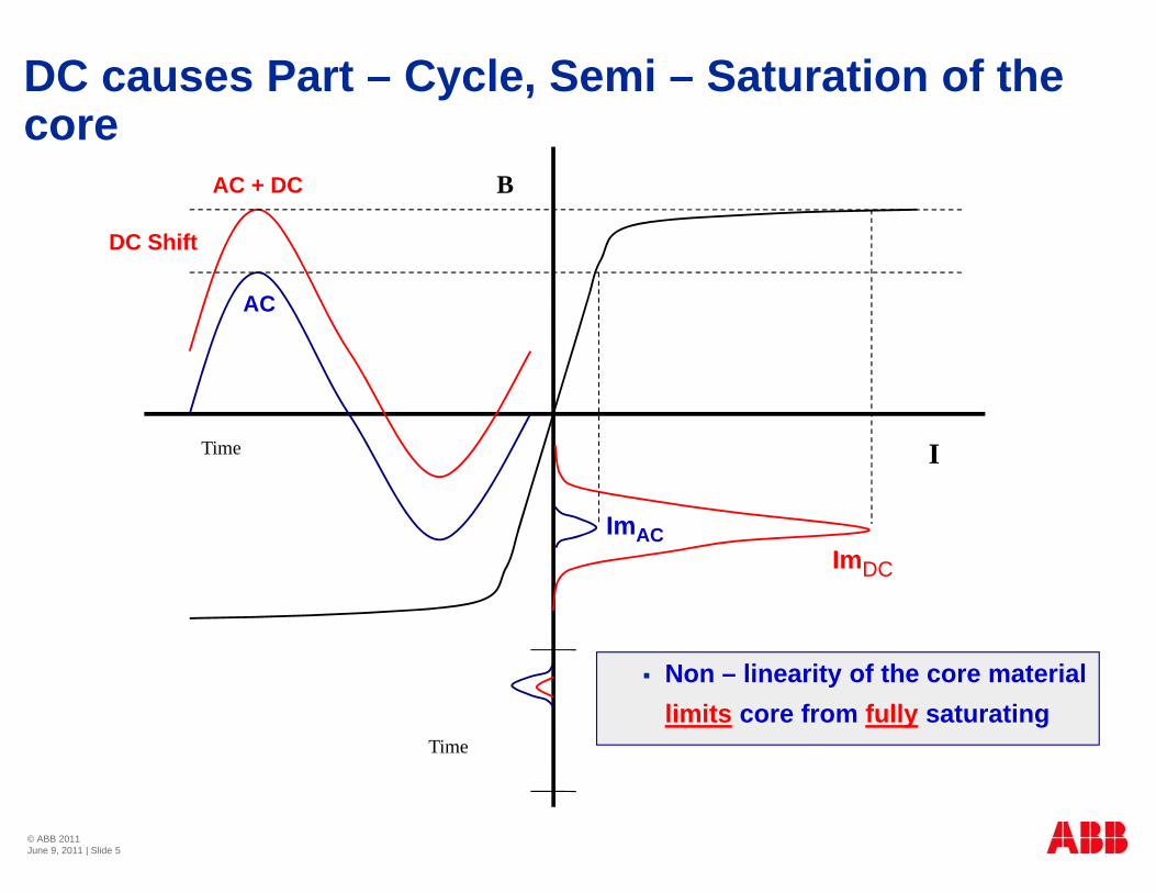
DC causes Part – Cycle, Semi – Saturation of the corecore

BAC + DC

DC Shift

AC

Time ITime I

ImImAC

ImDC

f

Time

Non – linearity of the core material limits core from fully saturating

© ABB 2011June 9, 2011 | Slide 5

Magnetizing current of a Transformer under effect of DC / GICof DC / GIC

% Exciting Current - 1 phase transformer - 20 Amps DC40%

Duration of the core semi-saturation

30%

35%

ent

depends on core type, transformer design, and magnitude of DC

25%

of L

oad

Cuu

re Typically 1/10th to 1/6th of a Cycle

15%

20%

g cu

rren

t, %

o

10%Exci

ting

0%

5%

© ABB 2011June 9, 2011 | Slide 6

-90 -60 -30 0 30 60 90 120 150 180 210 240 270Degrees

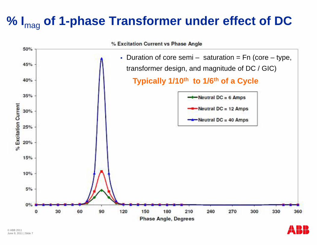
% Imag of 1-phase Transformer under effect of DC

Duration of core semi – saturation = Fn (core – type, Per Phase Currentstransformer design, and magnitude of DC / GIC)

Typically 1/10th to 1/6th of a Cycle

© ABB 2011June 9, 2011 | Slide 7

Main Factors affecting how much GIC would cause core semi saturationcore semi-saturation

Core Type

3 phase, 3 limb core vs. all other core typesp , yp

Number of turns in windings carrying the GIC

In 3 phase, 3 limb cores

Core operating Flux density Core operating Flux density

Distances between tank & core

© ABB 2011June 9, 2011 | Slide 8

DC Flux Path in different Core – Types

Core / Shell Form, 1 phaseCore Form, 3 phase, 3 limb

Core Form 3 phase, 5 limb

Shell Form, 3 phase, conventional

Shell Form 3 phase, 7 limbp

3 phase, 3 limb cores require much higher magnitudes of DC

© ABB 2011June 9, 2011 | Slide 9

to saturate compared to all other core – types All other core – types are basically equivalent

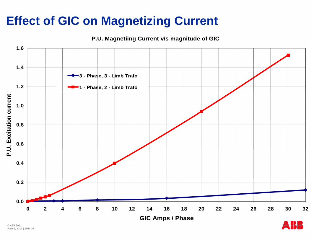
Effect of GIC on Magnetizing Current P.U. Magnetiing Current v/s magnitude of GIC

1.6

1.2

1.43 - Phase, 3 - Limb Trafo

1 - Phase, 2 - Limb Trafo

1.0

on c

urre

nt

0.6

0.8

U. E

xcita

tio

0.4

P.U

0.0

0.2

0 2 4 6 8 10 12 14 16 18 20 22 24 26 28 30 32

© ABB 2011June 9, 2011 | Slide 10

0 2 4 6 8 10 12 14 16 18 20 22 24 26 28 30 32

GIC Amps / Phase

Harmonic Content of magnetizing current associated with Core part cycle semi saturationassociated with Core part-cycle, semi-saturation

Harmonics Spectrum of Excitation current under DC Conditions16%

14% 3 - Phase, 3 - Limb Transformer

10%

12%

itude

1 - Phase Transformer

8%

arm

onic

s A

mpl

4%

6%

% H

a

0%

2%

© ABB 2011June 9, 2011 | Slide 11

0%60 120 180 240 300 360 420 480 540 600 660

Harmonic Frequency, Hz

Impact of core part-cycle, semi-saturation

Higher temperatures in windings leads structural parts and tank Higher temperatures in windings, leads, structural parts, and tank A high magnitude pulse of magnetizing current

High magnitude of leakage flux, rich in harmonics Higher eddy & circulating current losses

Some of the main core flux flows outside the core Tank wall heating

In shell form and in Core form transformers with 3 – limb cores Leakage flux => Tank walls Leakage flux => Tank walls

High winding circulating currents As a result of significant change in the leakage flux patterng g g p In some old shell form designs In some other transformers with particular design features

© ABB 2011June 9, 2011 | Slide 12

Characteristics of GIC Moderate magnitudes of current pulses over a few hours

Much higher short – duration current peaks g

Duration of highest magnitudes in an event is 1 – 2 minutes

© ABB 2011June 9, 2011 | Slide 14

Fig 4.8 in Meta-R-319 Report by J. Kappenman

Effect of GIC on Winding Hot Spot in a 1 – phase TransformerTransformer

Winding Hot Spot Temperature vs Time, 1-Phase Transformer 124

120

122

ree

C

116

118

pot T

empt

, Deg

r

112

114

Wdg

Hot

Sp

Idc = 50 Amps

Idc = 30 Amps

108

110

Idc = 30 Amps

Idc = 20 Amps

1080 5 10 15 20 25 30

Time, Minutes

Actual temperature rise is much lower due to short duration of highest peak of GIC

© ABB 2011June 9, 2011 | Slide 15

For a 2 – minute duration: Rise is 3, 4, and 6 C for GIC of 20, 30, and 50 Amps

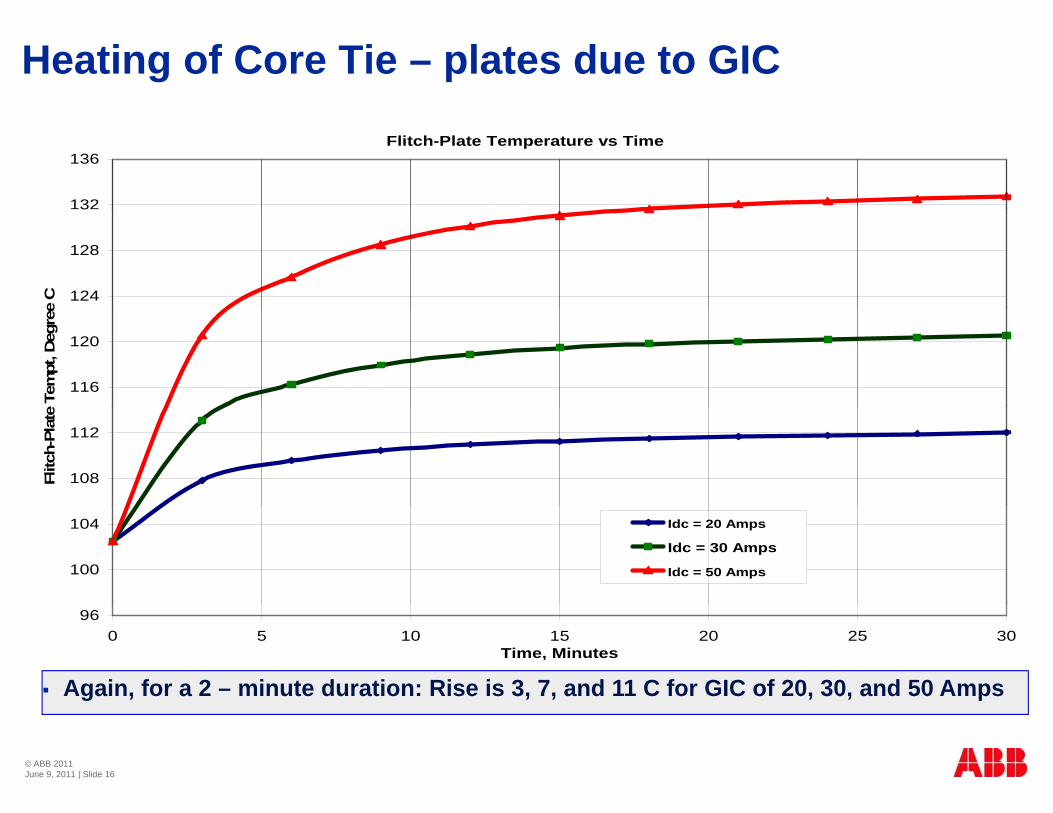
Heating of Core Tie – plates due to GIC

Flitch-Plate Temperature vs Time

132

136

124

128

3

e C

116

120

eTe

mpt

, Deg

ree

108

112

Flitc

h-Pl

ate

100

104 Idc = 20 Amps

Idc = 30 Amps

Idc = 50 Amps

Again, for a 2 – minute duration: Rise is 3, 7, and 11 C for GIC of 20, 30, and 50 Amps

960 5 10 15 20 25 30

Time, Minutes

© ABB 2011June 9, 2011 | Slide 16

Per phase GIC Wave – Form used for Thermal CalculationsCalculations

400 Amps 400 AmpsIdcIdc

About 5 times the levels experienced

at PSE&G Salem Generating Power

station in March, 1989

20 Amps 20 Amps 20 Amps

(0,0)30 2 30 2 30 Time, Minutes

© ABB 2011June 9, 2011 | Slide 17

Winding Hot Spot rise due to GIC in a 1 – phase TransformerTransformer Winding Hot Spot Temperature vs Time

160

120

140

e C

100

empt

, Deg

ree

60

80

g H

ot S

pot T

e

40Win

ding

0

20

© ABB 2011June 9, 2011 | Slide 18

00 10 20 30 40 50 60 70 80

Time, Minutes

Winding Hot Spot rise due to GIC in a 1 – phase TransformerTransformer Winding Hot Spot Temperature vs Time

160

120

140

e C

100

empt

, Deg

ree

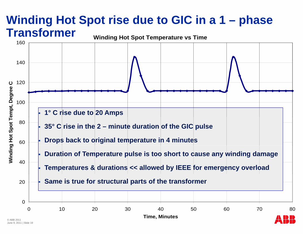
1° C rise due to 20 Amps

60

80

g H

ot S

pot T

e

35° C rise in the 2 – minute duration of the GIC pulse

Drops back to original temperature in 4 minutes

40Win

ding

Duration of Temperature pulse is too short to cause any winding damage

Temperatures & durations << allowed by IEEE for emergency overload

0

20 Same is true for structural parts of the transformer

© ABB 2011June 9, 2011 | Slide 19

00 10 20 30 40 50 60 70 80

Time, Minutes

Winding Temp. rise caused by a 2 – minute duration GICduration GIC

GIC L l Temperature TotalPer Phase Per 3 phase

100 300 5 116

GIC Level Temperature Rise, C

Total Temperature, C

200 600 9 120300 900 20 131400 1200 35 146400 1200 35 146

© ABB 2011June 9, 2011 | Slide 20

Measured Temp. rises in Windings / structural t d t DCparts due to DC

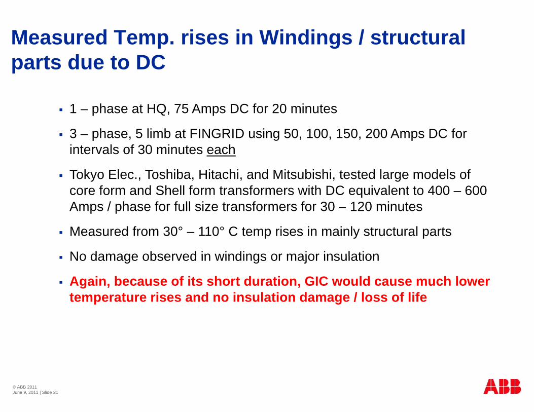
1 phase at HQ 75 Amps DC for 20 min tes 1 – phase at HQ, 75 Amps DC for 20 minutes

3 – phase, 5 limb at FINGRID using 50, 100, 150, 200 Amps DC for intervals of 30 minutes each

Tokyo Elec., Toshiba, Hitachi, and Mitsubishi, tested large models of core form and Shell form transformers with DC equivalent to 400 – 600 Amps / phase for full size transformers for 30 120 minutesAmps / phase for full size transformers for 30 – 120 minutes

Measured from 30° – 110° C temp rises in mainly structural parts

No damage observed in windings or major insulation No damage observed in windings or major insulation

Again, because of its short duration, GIC would cause much lower temperature rises and no insulation damage / loss of life

© ABB 2011June 9, 2011 | Slide 21

PSE&G Salem’s GSU Winding overheating during th 1989 GIC tthe 1989 GIC event

• An old Shell form transformer with an old design of LV windings

© ABB 2011June 9, 2011 | Slide 23

• Overheating: Caused by high Icirc as a result of core semi – saturation

Reported lead – overheating in S. Africa after a GIC E t

Reported cases were a number of same design transformers

Event

Reported cases were a number of same design transformers where the leads were heavily insulated with poor oil – flow in leads

Overheating caused charring of the inside wraps of insulation

Caused gassing but no failures

Overheating was found later during planned maintenance

Higher temperatures of leads due to high GIC is expectedg p g p

Part of the overheating is believed to have been there before the GIC event

© ABB 2011June 9, 2011 | Slide 24

Reported tank overheating in APS transformers ft GIC E tafter GIC Event

These were shell-form transformers

Wood slabs exist between core & tank walls

No oil cooling of these tank areas; not needed for normal

operating conditions

Temperature increase due to localized heating caused by stray p g y y

flux during a GIC event is expected (140° – 160° C, not 400° C)

H d Had no consequences

© ABB 2011June 9, 2011 | Slide 25

Consequences of Core part - cycle, semi -saturation on power systemssaturation on power systems

Causes a high magnitude of 1 – 2 msec – duration current Causes a high magnitude of 1 – 2 msec. – duration current pulse / reactive power (One / cycle) to flow in the system

This pulse causes the capacitive components on the p p psystem, such as static compensators, etc. to increase their currents and may become overloaded and trip, causing grid instabilityinstability

The current pulse is associated with high harmonics:

Resonance may occur and stability of the grid may be Resonance may occur and stability of the grid may be compromised due to the creation of virtual zero at some point and opening of lines.

Low % of 2nd order harmonic could send the wrong message of fault current to the differential relays

© ABB 2011June 9, 2011 | Slide 27

Factors that determine the magnitude of GIC

Affected location on Earth is dependent on location of the Affected location on Earth is dependent on location of the activity on the sun

A significant Sun – spot activity may, or may not, mean highA significant Sun spot activity may, or may not, mean high GIC in a particular location on Earth

Magnitude of GIC is a function of location on earth, resistance of the soil, and direction, height, and length of the transmission lines

Therefore 500 kV and 765 kV transmission lines tra elling Therefore, 500 kV and 765 kV transmission lines travelling long distances North – South are the most susceptible to the high levels of GIC

Based on above, only specific power grids, or parts of a power grid, would be susceptible to high levels of GIC

© ABB 2011June 9, 2011 | Slide 28

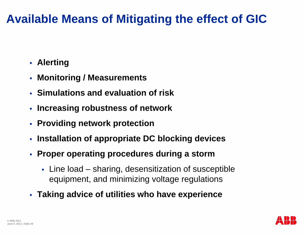
Available Means of Mitigating the effect of GIC

Al ti Alerting

Monitoring / Measurements

Simulations and evaluation of risk

Increasing robustness of network

Providing network protection

Installation of appropriate DC blocking devices

Proper operating procedures during a storm

Line load – sharing, desensitization of susceptible equipment, and minimizing voltage regulations

Taking advice of utilities who have experience

© ABB 2011June 9, 2011 | Slide 29

Effect of GIC on Power Transformers and Power SystemsSystemsConclusions / Summary

Because of its short duration even high levels of GIC would Because of its short duration, even high levels of GIC would not cause damaging overheating of neither windings nor structural parts of the large majority of power transformers

The failure of only one old shell form transformer of a very old winding design is confirmed to have been a consequence of GIC. All other failures, reported in the published literature o G C ot e a u es, epo ted t e pub s ed te atu eto have been caused by GIC, were not caused by GIC

Cases of lead and tank overheating, reported in the published literat re to ha e been ca sed b GIC ere either minorliterature to have been caused by GIC, were either minor heating of minimal consequences or were only partially caused by GIC.

The main impact of GIC is on the system instability it causes due to high levels of VARS and significant current harmonics as a result of transformer core part – cycle, semi – saturation.

© ABB 2011June 9, 2011 | Slide 30

as a result of transformer core part cycle, semi saturation.

Effect of GIC on Power Transformers and Power Systems

There are a number of means available for mitigating the effect

SystemsConclusions / Summary

There are a number of means available for mitigating the effect of GIC both on transformers and power systems

Manufacturers have different levels of competence in modeling technology and the know – how to evaluate transformer designs for the impact of GIC

It is possible to design transformers to be less vulnerable to It is possible to design transformers to be less vulnerable to part – cycle, semi – saturation during a GIC event Specifications of transformers to be subjected to high GIC

levels should include information on what level of GIC is expected at the transformer location

The issue should not be concern over “GIC causingThe issue should not be concern over GIC causing transformer failures”, rather: Transformers can be “susceptible to core saturation” and not to “failure”

© ABB 2011June 9, 2011 | Slide 31

NASA Perspective: Solar Shield – Forecasting Solar Effects on Power Transmissions Systems

(ccmc.gsfc.nasa.gov/Solar_Shield)

Pulkkinen, A., M. Hesse, S. Habib, F. Policelli, B. Damsky, R. Lordan, L.

Van der Zel, D. Fugate, W. Jacobs, E. Creamer

1

Contents• Some (general NASA Space Weather Laboratory) background.

• Solar Shield overview.

• Solar Shield forecasting system.

– Level 1 approach. The first tailored physics-based 2-3 day lead-time forecasts.

– Level 2 approach. The first tailored physics-based 30-60 min lead-time GIC forecasts.

• Coupling of the system to the SUNBURST research support tool.

• Summary.

2

Background

•NASA Space Weather Laboratory (GSFC) provides numerous state-of-the-art real-time space weather products for a wide variety of customers and collaborators.

• Space Weather Laboratory leverages NASA’s observational and modeling capacity to push the space weather forecasting envelope.

3

Background

• For a quick overview of the available space weather products, check iswa.gsfc.nasa.gov.

4

GIC forecasting challenge

5

Solar Shield overview• In Solar Shield, we developed a system to forecast space

weather effects on the North American power grid; initial development funded by NASA’s Applied Sciences Program.

• NASA/GSFC/CCMC and Electric Power Research Institute (EPRI) the key players.

• System has been running in real-time since February 2008.• DHS proposal was selected for contract award March 21,

2011.

6

System requirements (summary)

•Two-level GIC forecasts:– Level 1 providing 1-2 day lead-time.

– Level 2 providing 30-60 min. lead-time.

•Coupling to EPRI’s SUNBURST research support tool.

7

Used by the SUNBURST member utilities to monitor GIC.

Level 1 forecasts

8

Level 1 forecasts

April 3, 2008 9

Solar observations of eruptive events are used to compute “cone model” parameters. SOHO and STEREO data used.

Plasma “cone” introduced to the inner boundary of a heliospheric MHD model. Model propagates the disturbance to the Earth. Computations carried out at the Community Coordinated Modeling Center.

MHD output at the Earth used in a statistical model providing probabilistic estimate for GIC at individual nodes of the power grid. GIC forecast file is generated.

Pulkkinen et al. (Space Weather, 2009)

Level 2 forecasts

10

April 3, 2008 11

Lagrange 1 observations used as boundary conditions for magnetospheric MHD. NASA’s ACE data used.

Magnetospheric MHD model used to model the magnetospheric-ionospheric dynamics. Computations carried out at the Community Coordinated Modeling Center.

Magnetospheric MHD output used to drive geomagnetic induction and GIC code providing GIC at individual nodes of the power grid. GIC forecast file is generated.

Pulkkinen et al. (Annales Geophysicae, 2007)

Level 2 forecast example

12Oct 24, 2003

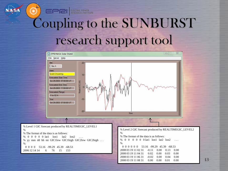
Coupling to the SUNBURST research support tool

13

% Level 1 GIC forecast produced by REALTIMEGIC_LEVEL1%% The format of the data is as follows: % 0 0 0 0 0 lat1 lon1 lat2 lon2 . . .% yy mm dd hh mi GIC1low GIC1high GIC2low GIC2high . . .%

0 0 0 0 53.16 -99.29 45.39 -68.532006 12 14 14 6 76 15 153

% Level 2 GIC forecast produced by REALTIMEGIC_LEVEL2% % The format of the data is as follows: % 0 0 0 0 0 0 lat1 lon1 lat2 lon2 . . .%

0 0 0 0 0 0 53.16 -99.29 45.39 -68.532008 03 19 11 02 31 -0.11 0.00 0.13 0.00 2008 03 19 11 04 31 0.02 0.00 0.03 0.00 2008 03 19 11 06 31 -0.02 0.00 0.04 0.00 2008 03 19 11 08 31 0.00 0.00 0.01 0.00

Summary

• Solar Shield system leverages NASA’s unique space weather modeling capabilities.

• Tailored two-level GIC forecasts generated for selected nodes of the North American high-voltage power transmission system.

• System is coupled to EPRI’s SUNBURST tool.

• System has been running in real-time since February 2008.

• Further development with DHS support underway.

• Much of the new forecasting capacity based on NASA’s science missions. Need better guarantee for data availability and continuity.

14

GMDTF Framing - nerc.com Disturbance Task Force... · AEP – Kwin Que. BottlierMagnitometer ......

Documents

Transcript of GMDTF Framing - nerc.com Disturbance Task Force... · AEP – Kwin Que. BottlierMagnitometer ......