ERIA Research Project Report 2010, No. 004

GGLLOOBBAALLIIZZAATTIIOONN AANNDD

IINNNNOOVVAATTIIOONN IINN EEAASSTT AASSIIAA

Edited by CHIN HEE HAHN DIONISIUS NARJOKO March 2011

i  

TABLE OF CONTENTS

Table of Contents i

List of Project Members ii

Acknowledgements iv

Executive Summary vi

CHAPTER 1. Globalization and Innovation in East Asia 1

Chin Hee Hahn, Dionisius Narjoko

CHAPTER 2. Sources of Learning-by-Exporting Effects: Does Exporting Promote Innovation?

20

Keiko Ito

CHAPTER 3. Direction of Causality in Innovation-Exporting Linkage: Evidence on Korean Manufacturing

68

Chin Hee Hahn and Chang-Gyun Park

CHAPTER 4. The Link between Innovation and Export: Evidence from Australia’s Small and Medium Enterprises

103

Alfons Palangkaraya

CHAPTER 5. Multinational Enterprises, Exporting and R&D Activities in Thailand 141

Archanun Kohpaiboon amd Juthathip Jongwanich

CHAPTER 6. Globalization and Innovation in Indonesia: Evidence from Micro-Data on Medium and Large Manufacturing Establishments

193

Ari Kuncoro

CHAPTER 7. Globalization, Innovation and Productivity in Manufacturing Firms: A Study of Four Sectors of China

225

Feng Zhen, Yanyun Zhao, Pierre Mohnen, Jacques Mairesse

CHAPTER 8. Trade Reforms, Competition, and Innovation in the Philippines 255

Rafaelita M. Aldaba

CHAPTER 9. Trade Liberalization and Innovation Linkages Micro-evidence from Vietnam SME Surveys

315

Nguyen Ngoc Anh, Nguyen Thi Phuong Mai, Nguyen Duc Nhat, Nguyen Dinh Chuc

CHAPTER 10. What Explains Firms’ Innovativeness in Korean Manufacturing?Global Activity and Knowledge Sources

341

Yong-seok Choi and Ki-wan Kim

CHAPTER 11. Knowledge Flows, Organization and Innovation: Firm-Level Evidence from Malaysia

370

Cassey Lee H. K.

CHAPTER 12. International R&D Collaborations in Asia: A First Look at Their Characteristics based on Patent Bibliographic Data

410

Naotoshi Tsukada and Sadao Nagaoka

ii  

LIST OF PROJECT MEMBERS

DR. SHUJIRO URATA (PROJECT SUPERVISOR): Professor, Graduate School of Asia-Pacific Studies, Waseda University, Japan; Senior Researcher Advisor to the Executive Director, Economic Research Institute for ASEAN and East Asia (ERIA), Indonesia.

DR. CHIN HEE HAHN (PROJECT LEADER): Associate Professor, Kyungwon University, Korea.

DR. DIONISIUS NARJOKO (PROJECT COORDINATOR): Researcher, Economic Research Institute for ASEAN and East Asia (ERIA), Indonesia.

DR. SADAO NAGAOKA: Professor, Institute of Innovation Research of Hitotsubashi University, Japan.

DR. NAOTOSHI TSUKADA: Research Associate, Institute of Innovation Research of Hitotsubashi University, Japan.

DR. YONG-SEOK CHOI: Associate Professor, Kyung Hee University, School of Economics, Korea.

DR.. KI-WAN KIM: Associate Research Fellow, Korea Development Institute, Korea.

DR. CHANG-GYUN PARK: Associate Professor, Chung-Ang University, Korea.

DR. CASSEY LEE HONG KIM: Senior Lecturer, School of Economics, University of Wollongong, Australia.

DR. RAFAELITA ALDABA: Senior Research Fellow, Philippine Institute for Development Studies (PIDS), Philippines.

DR. ARCHANUN KOHPAIBOON: Assistant Professor, Faculty of Economics, Thammasat University, Thailand.

DR. JUTHATHIP JONGWANICH: Assistant Professor, School of Management, Asian Institute of Technology, Thailand.

DR. JACQUES MAIRESSE: Professorial Fellow, UNU-MERIT, Netherlands; INSEE-CREST, France; National Bureau of Economic Research, USA.

DR. PIERRE MOHNEN: Professor, UNU-MERIT; Masstricht University, Netherlands.

DR. NYANYUN ZHAO: Professor and Dean, School of Statistics, Renmin University of China, China.

DR. FENG ZHEN: Postdoctoral Researcher, Bank of China; Chinese Academic of Social Science, China.

DR. NGUYEN NGOC ANH: Chief Economist, Development and Policies Research Center, Vietnam.

DR. NGUYEN THI PHUONG MAI: Senior Fellow, Development and Policies Research Center; National Institute for Science and Technology Policy and Strategy, Vietnam.

iii  

DR. NGUYEN DUC NHAT: Executiver Director, Development and Policies Research Center, Vietnam.

DR. NGUYEN DINH CHUC: Central Insitute of Economic Management, Vietnam.

DR. ALFONS PALANGKARAYA: Senior Research Fellow, Melbourne Institute of Applied Economic and Social Research and the Intellectual Property Research Institute of Melbourne, Australia.

DR. ARI KUNCORO: Professor of Economics, University of Indonesia, Indonesia.

DR. KEIKO ITO: Associate Professor, School of Economics, Senshu University

iv  

Acknowledgements

This report consists of all research papers from ERIA Microdata Research Project

of Fiscal Year 2010. The project is part of the broader ERIA’s research pillar on

Deepening Economic Integration. It addresses the theme of globalization and

innovation, with “Globalization and Innovation in East Asia” as the title of the

project and of this report. As indicated in the first chapter of this report, understanding

the process and determinants of innovation is unarguably a research and policy issue of

vast importance. Innovation is important for sustaining a country’s competitiveness in a

more globalized environment. All of the papers presented in three workshops over the

period of September 2010 to February 2011.

We incurred debts of gratitude to all members of the Project’s working group who

have actively contributed to the outcome of the research. We would like to also express

our sincere appreciation for the time willingly surrendered by all members to actively

communicate with ERIA and to participate in the three Project’s long workshops held in

Jakarta, Bali, and Bangkok over the course of the project.

Dr. Hahn and Dr. Narjoko owe a great intellectual debt to Professor Shujiro Urata

who provided excellent guidance throughout the course of the project. Professor Urata

has always been active in engaging in the research, from the very beginning at the

preparation stage, during the discussion of research papers in all three workshops, and at

the finalization step of the project.

We express our special thanks to Professor Fukunari Kimura, Chief Economist of

ERIA, for his encouragement and support for the project. Professor Kimura has always

been, and is still, one of the great supporters of ERIA Microdata Project. His idea of

inventing the unique ERIA’s Microdata research group is proven to be one of his

significant contributions, not only for the ERIA core economic research but also for the

academic literature and community in general.

We are greatly indebted to Mr. Hidetoshi Nishimura, Mr. Daiki Kasugahara, Mr.

Mitsuo Matsumoto, and Mr. Takeo Tsukuda, who have continuously and strongly

supported both the idea and the implementation of Microdata project. A successful

output delivery of the Microdata Project this fiscal year would not have been possible

without support from ERIA management.

v  

We are indeed grateful for the all reliable supporting staffs of ERIA, in particular

Maryclara Pondaag, Noviawaty, and Robertus Herdiyanto, for their tireless efforts to

help ensuring a successful delivery of the project. Last but not least, our sincere

appreciation to our colleagues, ERIA researchers, for their enthusiasms in the research

works of the project.

Chin Hee Hahn

Dionisius Narjoko

vi  

EXECUTIVE SUMMARY

Schumpeterian creative destruction or, in other words, innovation is the integral part

of a country’s economic growth. For developing countries, it would not be an

exaggeration to say that the challenges of economic development have been regarded by

policymakers as synonymous with the challenges of innovation: how to make

indigenous firms acquire new technologies and produce new products that they could

not previously. Therefore, understanding the process and determinants of innovation is

unarguably a research and policy issue of vast importance.

At the same time, a vast amount of previous studies have examined the causes and

as well consequences of globalization. These studies have shown, although with some

controversies remaining, that trade and/or investment liberalization has a positive effect

on growth and productivity of firms, industries, and countries involved.

Then, how is globalization related to innovation? Is globalization a cause of

innovation, or is innovation a cause of globalization, or both? Does increased trade and

investment liberalization lead to more innovation, or does it depress innovation activity?

In either case, what are the exact mechanisms? These are some of the most important

questions that this report aims to address. These are some of questions that this report

attempts to answer.

This report, of course, is not the first that explores globalization-innovation linkage.

In fact, this topic is at least decades old. Previous studies on trade and growth have

examined at least the following main channels through which trade affects growth:

knowledge spillovers, increased competition, and larger market size. And these

channels are either directly or indirectly related to firm’s innovation activity.

Traditional argument goes that, for example, if trade or investment liberalization

facilitates knowledge spillovers, this will reduce the cost of research and development

(R&D) or raise the rate of return to such activity, leading to increased innovation.

Increased market size associated with trade raises the rate of return to innovation

activity. Enhanced competition through trade may exert pressure on firms to innovate,

or it could hurt the incentive to innovate by squeezing out the ex-post profit from a

successful innovation. There are numerous empirical studies that examine these

vii  

channels in detail. In this regard, this report is, in some sense, a revisit to an old issue.

This report collects many interesting findings based on the papers/studies done to

cover many countries in East Asia region. Along with its wide international coverage,

this project utilizes micro-level data at plant, firm, or product level. While innovation

may be an old topic, there have not many studies in the literature that utilize data at this

micro level, addressing the innovation linkage to globalization, and focusing on the

most rapidly growing region in the world. There are, therefore, rich insights that one

can draw from all papers in this report.

In terms of key findings, there are many papers that confirm the positive impact of

exporting on firm innovation activities and performance. While almost all papers in this

report provide evidence for this, there are three papers that specifically show this

evidence in the context of the role of innovation in the exporting-productivity

relationship. In particular, the evidence supports to the existence of ‘learning-by-

exporting’ behavior, which is one possible explanation for this relationship. The

Japanese case study on this subject shows that the first-time exporters indeed increase

their R&D expenditure immediately after they export, albeit the increase depends on the

export-market destinations. One of the Korean studies and the Australian study also

support the positive exporting-innovation relationship. The former shows that exporting

promotes the creation of new product while the latter reveals the behavior that exporters

in services sector do indeed increase their process-innovation activities. All of these

studies, in addition to establishing the positive exporting-innovation linkage, also show

that the positive impact is further translated to superior firm performance.

Firm’s R&D activities are the focus of the other three chapters in the report. As

input of innovation outcome, R&D activities provide useful information about the

extent of knowledge creation. Key findings within this subject are related to the role of

foreign ownership in affecting firm innovation. The first is multinational enterprises

(MNEs) tend to import their technology from their parent companies, resulting in rather

low innovation activities of these MNEs in their host countries. The Thai and Chinese

studies highlight this observation. This rather discouraging finding, however, does not

mean that there is no positive effect of MNE presence on R&D or innovation process.

In fact, as indicated by the Thai study, as well as the Indonesian study, the presence of

MNEs is suggested to stimulate locally owned firms to conduct R&D. In other words,

viii  

there exist what so-called the ‘R&D spillovers’ from MNEs presence.

The Indonesian study also finds an interesting fact of a positive relationship

between the acquisition of new machinery and the extent of R&D expenditure. In other

words, at least for Indonesia in this case, the ups and downs of firm innovation output

are closely related to the ability of the firm in acquiring new machinery.

Other chapters examine the impact of globalization on innovation through

competition link. The Philippines and Vietnamese studies address this subject. The

Philippines study finds that trade reforms increases the extent of competition in

domestic markets. Reduction in tariff is related to reduction in profitability. This study

further finds that higher competition stimulates R&D. Thus, overall, trade liberalization

positively affects R&D through product market competition channel. All these findings

are generally the same even after it takes into consideration the firm selection impact as

a result of much tighter competition (i.e., firm entry and exit). Consistent finding on the

impact of competition is shown by the Vietnamese study. Tight price competition is

found to increase the likelihood of Vietnamese small and medium enterprises (SMEs) to

engage in R&D.

Globalization and knowledge creation and absorption is closely related. Another

Korean paper shows that positive innovation premium can be accounted for by both the

utilization of existing knowledge and active investment in new knowledge. The degree

of importance for each of these knowledge sources, however, is different, depending on

the characteristics of the global activity that a firm involves in. Investing in new

knowledge seems to be more important than utilization of existing knowledge in

explaining the premium of the non-MNE exporters and domestic MNE parents with

export participation. In contrast, foreign MNE affiliates that participate in export

markets seems to utilize existing knowledge more than investing in new knowledge in

generating their positive innovation premium. The paper utilizing the Malaysian

innovation survey, meanwhile, attempts to draw whether there is relationship between

various aspect of organization and innovation. This study finds it to be a complex one.

Different types of internal and external knowledge flows are likely to be driven by

different organizational variables. For example, while knowledge flows from other

companies within the same group are determined by whether or not the firm is a

subsidiary. Meanwhile, examining the impact of international research collaboration

ix  

involving patent registered in Korea, China, and Taiwan, another study in this report

finds that international co-inventions are strongly associated with more science linkage,

with higher quality of patent, and larger group of research team.

The research conducted by all papers in this project asserts that globalization

encourages firm-level innovation. This policy implication is very important in the

context of the usual approach that countries rely on R&D subsidies. The key message

coming out from this research, therefore, is the existence of an alternative way for a

country to promote innovation, which is done by, and through, maximizing the benefit

from globalization.

There are more specific policy-implications implied by this broad message. First,

policy to promote exports encourages firm innovation; hence, policy to assist firms to

export more, as well as to make more firms to engage in exports, seems warranted. A

number of findings on the positive relationship between exporting and innovation

activities and/or performance support this policy implication. Second, policies for

higher foreign involvement should be encouraged. The justification of this comes

mostly on the evidence on the existence of ‘R&D-spillovers’ impact on domestically

owned firms, from the presence of MNEs.

Third, keeping in track with ongoing trade liberalization and maintaining a

relatively open trade regime is suggested. A high degree domestic market competition

drives firms to always engage in innovative-enhancing activities, through the ability of

the competition to create a contestable market situation. The findings from the

Philippine study provide some evidence to support this. Having a liberalized trade

regime could even be more beneficial if it is put in a framework of deepened integration

of a country in Southeast and East Asia regions. The case study of Thai manufacturing

in this report underlines this in the context of linking firms the already-established

international production networks in these regions. The Thai study finds positive

relationship between participation in the production networks on greater R&D activities

by firms.

Fourth, findings from the research suggest that globalization seems to also benefit

SMEs – not only large firms. This is encouraging given the common perception of

unfavorable impact of globalization on SMEs. But there is more on this; how does one

devise policies to materialize this benefit? The Australian study in this report suggests

x  

that, at least conceptually, the policy is to gear SMEs to learn more about process

innovation – rather than product innovation – from utilizing globalization forces.

1

CHAPTER 1

Globalization and Innovation in East Asia

CHIN HEE HAHN

Kyungwon University

DIONISIUS NARJOKO

Economic Research Institute for ASEAN and East Asia (ERIA)

2

1. Background and Objective

This report consists of the papers submitted to ERIA’s research project

“Globalization and Innovation in East Asia” in fiscal year 2010. This project aims to

examine the relationship between globalization and innovation, as well as the impact of

various policies on innovation process and/or its outcomes in a globalized economic

environment, utilizing various firm-, plant-, and/or product-level micro datasets for East

Asian countries.

As is well understood, the process of Schumpeterian creative destruction or, in

other words, innovation, is an integral part of economic growth in every country.

Particularly for developing countries in East Asia, but also in other regions, it would not

be an exaggeration to say that the challenges of economic development have been

regarded by policymakers as synonymous with the challenges of innovation: how to

make indigenous firms to acquire new technologies and produce new products that they

could not previously. It is therefore clear that understanding the process and

determinants of innovation is unarguably a research and policy issue of vast importance.

At the same time, numerous studies have examined the causes and consequences of

globalization. These studies have shown, although with some controversies remaining,

that trade and/or investment liberalization has a positive effect on the growth and

productivity of the firms, industries, and countries involved. Partly as a result of the

progress in our knowledge in this field, openness of their trade and investment regimes

is considered as a key necessary condition for the economic growth and development of

developing as well as developed countries.

So, how is globalization—a process of closer economic integration by way of

increased trade, foreign investment, and international labour mobility—related to

innovation? Is globalization a cause of innovation, or is innovation a cause of

globalization, or both? Does increased trade and investment liberalization lead to more

innovation, or does it depress innovation activity? In either case, what are the exact

mechanisms? These are some of the most important questions that this report aims to

address.

3

There are numerous additional issues that bear on this report. These include, for

example, how innovation activity is organized within multinational enterprises (MNEs),

and whether, and precisely how, globally engaged firms (either directly through foreign

direct investment (FDI) or trade, or indirectly through interactions with foreign firms)

differ in innovation activity and innovation outcome. Other issues are the causes and

consequences of the globalization of innovation activity itself, and the role of firm

characteristics and/or firm-heterogeneity in the trade-innovation linkage. Then there are

the roles of competition in the trade-innovation nexus, and of openness policies in

innovation policies and vice versa. Then, how a country’s level of development,

protection of intellectual property, and technical standards and regulations, affect the

relationship between globalization and innovation, and so on. Some of these questions

are also addressed by the chapters included in this report.

Of course, this report is not the first to explore the globalization-innovation linkage.

In fact, this topic is at least decades old.1 Previous studies on trade and growth have

examined the following main channels through which trade affects growth: knowledge

spillovers, increased competition, and larger market size. And these channels are either

directly or indirectly related to the firm’s innovation activity. Traditional argument

goes that, for example, if trade or investment liberalization facilitates knowledge

spillovers, this will reduce the cost of R&D or raise the rate of return to such activity,

leading to increased innovation. Increased market size associated with trade raises the

rate of return to innovation activity. Enhanced competition through trade may exert

pressure on firms to innovate, or it could hurt the incentive to innovate by squeezing out

the ex-post profit from a successful innovation. There are numerous empirical studies

that examine these channels in detail. In this regard, this report is, in some sense, a

revisit to an old issue.

However, we think that the primary distinguishing feature of this report is the use of

micro-data. Although trade and innovation may be an old topic, to the best of our

knowledge, there are not many previous studies that utilize firm- or plant-level micro

data and examine the linkage between globalization and innovation, particularly in East

Asian countries. In addition, most chapters in this report use a variety of data sources

1 See Helpman (2004) for an excellent review of the literature on this topic.

4

and employ explicit measures of innovation input and innovation outputs (process or

product). We think that the use of micro data allows us to clarify further the

relationship between globalization and innovation, which studies based on aggregated

data were unable to do. Furthermore, we think that using micro data allows us to

examine the possible roles of firm characteristics, such as productivity, size, and other

technical characteristics, in the globalization-innovation linkage.

The use of micro data, as well as recent developments in academic literature (and in

the real world), make this report not just a revisit of the old issue but rather a revisit of

the old issue in a new context and with a new approach. It is clear that globalization

these days has new features compared with globalization, say, before the 1980s. The

prime example of this is the so-called fragmentation of production or internalization of

production. It is well known that the evolution of this process has been most

pronounced in East Asian countries. So, these days, FDI directed to the developing East

Asian region as well as FDI originating from developed East Asian countries, such as

Japan, frequently involves the relocation of a certain production process in search of a

lower production cost. Although there are increasing numbers of studies on the causes

and consequences of this so-called vertical FDI, studies examining the consequences of

this FDI on the host and home country firm’s innovation activity are rare. Some of the

chapters in this report bear on this issue.

Recent developments in heterogeneous firm trade literature also provide new

insights and a theoretical framework for some of the chapters in this report. Earlier

version of the heterogeneous firm trade theory, pioneered by Melitz (2003), helped not

only to clarify the channels through which the benefits of globalization are materialized

(reallocation of resources across firms within industries and/or across products within

firms and/or across different technologies), but also identified firm-level characteristics

(primarily productivity) that matter in shaping the relationship between globalization

and aggregate growth and productivity. More recent literature has incorporated the

firm-level innovation decision into the model, and examined various dynamic

relationships that could exist among trade, innovation, and productivity. For example,

this literature implies that there exists a bi-directional causal relationship between trade

and innovation and that firm level productivity is both a cause and a consequence of

5

past trade and innovation activities. Some of the chapters in this report use this

theoretical framework in their empirical analyses.

It is our belief that examining the trade and innovation linkage in a new context and

with new approach, and addressing the important questions discussed above can provide

us with rich policy implications. For example, many chapters in this report provide

strong empirical evidence that a firm’s globalization activities are at least a determinant

of its innovation inputs and outputs or, in some cases, that there exists a bi-directional

causal relationship between globalization and innovation. This suggests a strong case

for coordination between trade/investment liberalization policy on one hand and

innovation policy on the other. In view of the often observed reality that these two

policies are separately planned and governed by different ministries, this report’s

findings have potentially profound implications.

Below, we provide a synopsis of what follows and summarize the main policy

implications that arise out of this report.

2. Report Structure and Main Findings

This report consists of eleven papers that address the globalization-innovation

issues in nine countries, namely Japan (two papers), Korea (two papers), China, Taiwan,

Australia, Thailand, Indonesia, Malaysia, the Philippines, and Vietnam. These papers

can be classified into four groups according to more specific themes, that is, (i)

exporting, innovation, and productivity, (ii) the firm’s R&D decision and globalization,

(iii) trade liberalization, competition, and innovation, (iv)globalization of R&D,

organization, and knowledge flows.

2.1. Exporting, Innovation, and Productivity

The first three chapters address the role of innovation in the relationship between

exporting and productivity, in the context of learning-by-exporting and the self-

selection hypothesis. In Chapter 2, Ito addresses the role of innovation in the context of

the learning-by-exporting hypothesis. She asks whether the effect of learning-by-

6

exporting on innovation exists and, subsequently, whether and how the impact of

exporting on innovation affects productivity. The paper attempts to find answers to

these questions by examining the behavior and performance of first-time exporters in

Japanese manufacturing. Ito’s paper, therefore, not only seeks evidence for the positive

impact of learning-by-exporting on innovation but also moves deeper to find insights on

the source of the learning-by-exporting.

In her investigation, Ito finds that the first-time exporters are able to increase their

sales and employment growth to a greater extent than those serving domestic markets.

More importantly, the decision to begin to export evidently promotes innovation; she

finds that the first-time exporters record an increase in R&D intensity and volume. In

going deeper into the mechanism of learning-by-exporting, Ito examines whether there

are differences in the performance of innovation and other performance variables,

arising from engaging in exporting to different destinations. She finds that starting to

export to North America/Europe has larger positive effects on productivity than starting

exporting to Asia. This difference is also observed for the other performance variables

(i.e., sales and employment growth), innovation variables, and some characteristics of

the firms. Ito ascribes this to differences in absorptive capacity; i.e., the first-time

exporters to North America/Europe have greater absorptive capacity than those

exporting for the first time to Asia.

Chapters 3 and 4 examine how innovation affects the export-

productivity/performance link. Unlike the previous chapter, these chapters examine the

effect in the context of the two hypotheses. Specifically, these chapters examine the

possible two directional relationships between export participation and innovation.

Hahn and Park in Chapter 3 utilize a rich combination of plant- and product-level data

from Korean manufacturing in their investigation. Unlike the previous studies, however,

Hahn and Park adopt a rather different approach in defining product innovation. That is,

they use plant-and-product matched data to distinguish two types of product innovations:

those that are new to the plant (termed ‘product addition’) and those that are new to the

Korean economy (termed ‘product creation’). The former tends to capture the product

cycle phenomenon or international knowledge spillover, while the latter reflects

imitation by domestic competitors or the process of domestic knowledge diffusion.

7

Product creation could mean product addition although this does not necessary work the

other way around.

Hahn and Park find evidence to support the learning-by-exporting hypothesis for

the role of innovation in the export-productivity relationship. Using propensity score

matching, they find a statistically significant positive impact of exporting on product

creation. They cannot however infer the existence of this relationship when innovation

is defined by product addition; the impact of exporting on product addition is not

statistically significant, albeit showing the same (i.e., positive) sign. Hahn and Park

meanwhile, are not able to find evidence to support the selection hypothesis. More

specifically, they cannot find any significant effect of innovation – for both product

creation and addition – on exporting. Hahn and Park extend their investigation by using

the vector autoregressive (VAR) method. This route is taken in order to examine the

dynamic interdependence between export and innovation, as well as productivity. The

key results from it are consistent with the key finding that exporting significantly affects

product creation. The finding from the VAR indicates that this impact is quite

persistent; it takes more than five years for the impact on product creation to die out.

The VAR results, in addition, show that productivity significantly and positively affect

both exporting and product creation.

Palangkaraya in Chapter 4 conducts his investigation on the direction of causality

using firm level data from Australian small and medium enterprises (SMEs). His

investigation also specifically looks at the direction of causality for the group of new

exporters and new innovators; this is done to ensure the robustness of his investigation

results. It is worth mentioning that Palangkaraya’s analysis is rather different from the

other research papers in this report in terms of sectoral coverage in that it takes in not

only manufacturing firms but also enterprises in the services and other non-

manufacturing sectors. This offers a distinct value added to the research on the subject,

considering the argument that the lessons from the usual samples from the

manufacturing sector may not be valid for the other sectors.

Unlike Hahn and Park, Palangkaraya finds evidence that the relationship between

exporting and innovation runs in both directions. However, this only appears for

process innovation and in the services sector; not for product innovation and not in

manufacturing or other non-manufacturing sectors. The investigation also finds that the

8

positive two-way relationship varies across industries. In his interpretation,

Palangkaraya attributes all these results to the uniqueness of the innovation

characteristics of SMEs and the importance of services in the Australian economy.

More specifically for the former, process innovation matters more than product

innovation because SMEs are usually financially constrained and product innovation is

arguably substantially more expensive than process innovation.

2.2. Firms’ R&D Decisions and Globalization

Firms’ research and development (R&D) activities are the focus of the next three

chapters. As an input resulting in an innovation outcome, R&D activities provide useful

information about the extent of knowledge creation. The next three chapters examine

whether and how globalization affects a firm’s R&D performance. In Chapter 5,

Jongwanich and Kohpaiboon examine the roles of multinationals (MNEs) and exporting

in determining the decision to carry out R&D, and the actual intensity of R&D activities,

in firms in the Thai manufacturing sector, utilizing the most recent (i.e., 2006) industrial

census data. Unlike the other studies that measure different types of R&D in their total

value terms, Jongwanich and Kohpaiboon disaggregate R&D activities into three

categories, namely: (i) R&D leading to improved production technology, (ii) R&D

leading to product development, and (iii) R&D leading to process innovation. This

chapter examines not only the direct effect of MNEs on R&D activities, but also the

indirect effect of MNEs on the presence and intensity of R&D in locally owned plants

(termed here ‘R&D spillovers’).

Jongwanich and Kohpaiboon find that globalization, through exporting and FDI,

can play a role in encouraging firms to commit to R&D investment. The role played by

FDI, however, seems to be different from that played by export. They found that the

R&D propensity of MNE affiliates is lower than that of locally owned firms. This

suggests that MNE affiliates in Thailand prefer to import technology from their parent

companies rather than investing in R&D in the host country (Thailand). Nonetheless,

this does not mean that there is no effect arising from MNE presence on firm R&D

propensity and intensity. In fact, Jongwanich and Kohpaiboon find evidence that the

presence of MNEs stimulates locally owned firms to conduct R&D activities.

Jongwanich and Kohpaiboon also find that firms participating in international

9

production networks are more active than those are not participating. As for the role of

exporting, Jongwanich and Kohpaiboon find a positive and significant impact on R&D

activities, from being in production networks, although this is limited only to R&D in

product development. They do not find a significant impact for the other forms of R&D

(i.e. R&D leading to improvement in production technology and R&D leading to

process innovation). This finding implies that entering export markets helps firms to

learn more from competing products, and from customer preferences, but their

information relating to improving production technology and process innovation is still

limited.

In Chapter 6, Kuncoro examine the globalization determinants of the decision to

invest in R&D and the intensity of R&D expenditure, of medium-and large-sized

manufacturing firms in Indonesia. Kuncoro considers export participation, foreign

investment, and trade protection as the variables that represent globalization. In

addition, he looks at the impact of spatial concentration of MNEs in affecting the firm’s

R&D investment decision and expenditure. Kuncoro uses data from the period of mid

1990s to mid 2000s in his empirical investigation.

Kuncoro finds that being an exporter significantly affects a firm’s decision to invest

in R&D, as well as the extent of the firm’s R&D expenditure. As for the importance of

foreign ownership, Kuncoro finds that it is an important determinant only of the firm’s

R&D investment decision; he finds that it is not an important factor in determining the

amount of R&D expenditure that the firm commits. In terms of testing the potential

R&D spillover effect arising from concentration of MNEs in a location, he finds that

R&D activities tend to be higher in big urban areas; not in a specialized or agglomerated

location. In his interpretation of the findings related to foreign ownership and the

presence of MNEs, he asserts that there may be needed a critical mass of MNEs in a

location, or in an agglomeration area, for these MNEs to have meaningful impact in

terms of innovation or R&D performance. Another element of globalization, trade

protection, is found to be negatively related to a firm’s R&D investment decision and

expenditure. In other words, lowering the protection or trade barrier will create a

positive impact on R&D activities. In addition, Kuncoro interestingly finds a positive

relationship between R&D expenditure and investment in new machinery. He asserts

that investment in new machinery may reflect another indirect effect of globalization on

10

the firm’s innovation performance or R&D activities; it may reflect the desire of a firm

to remain competitive, which can be accomplished by installing new machinery,

bringing new technology.

Chapter 7 by Mairesse et al. examines the determinants of decisions on R&D and

its intensity in four major Chinese manufacturing sectors, namely, textiles, apparel,

transport equipment, and electrical equipment. The authors examine the determinants in

the framework of the Crepon, Duguet, Mairesse (hereafter CDM) structural model that

links between innovation input, innovation output, and performance. Hence, in addition

to examining the R&D decision and R&D intensity, they also examine how R&D

intensity affects innovation output, as well as how innovation output determines

performance. Exporting and foreign ownership are included in the determination of the

R&D decision and R&D intensity as well as in the determination of innovation output

and performance. They use the data from manufacturing censuses conducted in 2005

and 2006.

Mairesse et al. find evidence that exporting increases the likelihood of firms making

an R&D investment, and the level of R&D intensity; however, they find this to be the

case only in the textile industry. They find conflicting evidence in the case of the

electronic equipment industry. Given the fact that many firms in this industry have

some share of foreign ownership, Mairesse et al. interpret this finding as a reflection of

the position that much R&D activity is carried out by parent companies located in other

countries, not in China as the host country. Their interpretation is consistent with their

other finding which suggests that foreign firms tend to innovate less than other firms in

China, compared to the state-owned ones. In addition, to all these, Mairesse et al.

interestingly find that exporting does improve innovation output, and here specifically

in terms of improving new products.

2.3. Trade Liberalization, Competition, and Innovation

Chapters 8 and 9 address the impact of trade and investment liberalization on

innovation. Aldaba in Chapter 8 examines this issue in the case of manufacturing firms

in the Philippines, utilizing firm-level panel data over the period 1996-2006. In her

examination, she asks the following questions: what is the impact of the removal of

trade barriers on firms’ innovative activities? And does an increase in competition

11

arising from trade reforms lead to increases in innovation? The analytical framework

adopted by Aldaba postulates that the trade-liberalization relationship operates through

the competition channel; hence, the impact of trade liberalization is examined through a

two-stage approach where competition is endogenous. She also takes into consideration

the selection, or firm-dynamic impact of competition, in her empirical model.

Aldaba finds that trade reforms (i.e. reduction of tariff and/or non-tariff barriers)

conducted several times in the Philippines from the 1990s to the 2000s have had a

strong impact on the Philippines’ manufacturing sector, by increasing the extent of

competition in domestic markets. The tariffs are found to be positively related to the

price-cost margin. This is the finding from the first step of her econometric estimation.

From the second step of the estimation, Aldaba finds that profitability is negatively

related to R&D expenditure. In other words, higher competition stimulates R&D. Thus,

overall, trade liberalization positively affects R&D through the product market

competition channel. All these findings are generally the same even after she controls

for firm entry and exit, which are proxies for the industry selection impact arising from

competition. Further, from the results of her estimation in the ‘mixed’ sector (i.e. a

broad sector group that consist of mostly exporting and importing industries), she finds

that the net-entry variable is negatively related to profitability. Together with a negative

relationship between profitability and R&D expenditure, this indicates that as more

firms exit (presumably the inefficient ones), the surviving firms tend to engage in R&D,

in order to out-compete the new firms entering the market.

In chapter 9, Nguyen et al. examine the determinants of innovation by Vietnamese

SMEs in the context of increased competition as a result of rapid trade expansion in the

2000s. Nguyen et al. use data of 2007 and 2009 from the Vietnam SME Survey. The

years of the data are chosen to capture the period when Vietnam experienced rapid trade

liberalization. Unlike the approach taken by other studies, Nguyen et al. use

information on pricing strategy to capture the extent of competition among firms. The

use of this information is really driven by the availability of the information in the data

set used.

Nguyen et al. find some importance of competition effects, both domestic and

international. Specifically, matching the price of competitors has a positive impact on

product innovation using the 2007 data and on product improvement using the 2009

12

data. As for the impact of international competition, they found that the pressure from

foreign firms – in terms of price set by them – evidently improves all kinds of

innovation activities by the Vietnamese SMEs (i.e. product innovation, product

modification, and process innovation). This finding, however, slightly differs when the

experiment uses 2009 data. Nguyen et al. not only address the globalization impact

through the competition channel, but also further test whether linkages with foreign

firms help the SMEs to increase their innovation activities. They find rather convincing

evidence on this, using both years of the data and the other innovation activities they

consider.

2.4. Globalization of R&D, Organization, and Knowledge Flows

Chapter 10 by Choi and Park examines the link between the “innovation premiums”

from engaging in global activity and sources of knowledge in Korean manufacturing.

They first examine whether these premiums exist and, based on their findings on this,

they examine what sources of knowledge could explain the premiums. To capture the

premiums, Choi and Kim compare the innovation output of various types of firms that

engage in global activities with the innovation output of domestically-focused firms.

Global activities of the firms are defined according to their export participation and/or

their FDI engagement. Choi and Kim measure innovation output in terms of product or

process innovation (or both of these) as well as number of patents. They also consider

two groups of knowledge sources, namely investment in new knowledge and utilization

of existing knowledge (either from inside or outside firms). This paper draws data from

Korea’s Innovation Survey conducted in 2002, 2005, and 2008, as well as data from the

Kore EXIIM bank.

Choi and Kim show that there indeed exists a premium in terms of innovation

output from engaging in global activities. The comparison they make shows that

performance in generating innovation outputs is the highest for firms that export and

have foreign ownership participation, but is the lowest for purely domestic firms (i.e.

domestic firms without any exports and without any foreign ownership). In their further

investigation, Choi and Kim find that the positive innovation premium can be accounted

for both by the utilization of existing knowledge and by active investment in new

knowledge. The degree of importance of each of these knowledge sources, however, is

13

different, depending on the characteristics of the global activity that a firm is involved

in. Investing in new knowledge seems to be more important than utilization of existing

knowledge in explaining the premiums of the non-MNE exporters and the domestic

MNE parents with export participation. In contrast, foreign MNE affiliates that

participate in export markets seem to utilize existing knowledge more than investing in

new knowledge in generating their positive innovation premium. Another important

finding is that, when Choi and Kim analyze product and process innovation separately,

they find that utilization of existing knowledge and investment in new knowledge are

equally important in explaining the positive premium for product innovation. However,

only information from existing knowledge seems to be important in explaining the

premium for process innovation.

Chapter 11 by Lee is another paper in this report addressing the issue of knowledge

flows in innovation. Lee uses Malaysian manufacturing as the case study in his paper.

In his research, Lee gauges the determinants of knowledge flows in the decision to

invest in R&D as well as in the intensity of a firm’s R&D activities. This is the first

step in his investigation. Measures of R&D activity considered by this paper are: (i) in-

house R&D activity, (ii) acquisition of machinery, equipment, and software, and (iii)

training. Further, in the second step he attempts to find some evidence on whether the

variation in the extent of knowledge flows can be explained by firm organizational

factors. He considers various organizational factors classified into three broad groups

according to the characteristics of the factor, namely, (i) vertical boundary of firm, (ii)

ability to adapt to changing environment, and (iii) collaborative activities with external

parties.

Lee incorporates globalization into each of these steps by introducing variables that

identify a firm’s export participation and the existence of foreign participation in the

firm’s ownership structure. Lee also differentiates collaborative variables – as one of

the groups of organizational variables – according to the domestic or foreign

collaborative partners; this is another way of incorporating globalization into his

knowledge flows and organization equation.

Lee finds evidence that establishes the relationship between knowledge flows and

innovation. However, the extent and direction of the relationship is likely to depend on

the type of innovation activities. For in-house R&D, for example, the knowledge flow

14

from other firms within the same group of companies is negatively related to the

decision to undertake this activity. Also, there is evidence of less emphasis on in-house

R&D investment if knowledge flows from customers are of high importance. In the

case of the acquisition of machinery, equipment, and software, external knowledge

flows are important, especially those coming from suppliers, customers, competitors,

and consultants. As for the importance of globalization-related variables (i.e. exporting

and foreign ownership) in determining these activities, Lee finds them to be relatively

insignificant. Lee only finds a positive impact from globalization when the innovation

activity considered is training, and the globalization variable introduced is exporting.

Specifically, exporting is associated with higher investment in training.

As for the relationship between knowledge flows and various aspects of

organization, Lee finds it to be a complex one. Different types of internal and external

knowledge flows are likely to be driven by different organizational variables. For

example, while knowledge flows from other companies within the same group are

determined by whether or not the firm is a subsidiary, as well as by cooperation

involving foreign customers and foreign private research centers, external knowledge

flows seem to be determined only by some of the variables that reflect the firm’s ability

to adapt to its changing environment (i.e. improvement in the quality of goods and

services, improvement in employee satisfaction and reduction in employee turnover).

Despite this complexity, Lee finds evidence to support the positive role of globalization

in determining the extent of knowledge flows; the globalization-related variables, i.e.

exporting and foreign ownership, are generally found to be important for certain types

of external knowledge flows, particularly those originating from customers.

The last of the chapters of this report, by Nagaoka and Tsukada, addresses

international collaboration in research. Specifically, they analyze whether and how

international research collaboration affects invention in three countries, namely Korea,

China, and Taiwan. In their investigation, they focus on patents registered in the patent

office in these countries as well as in the US Patent Office.

Nagaoka and Tsukada find that international co-inventions are strongly associated

with more science linkage; that is, more references to scientific literature in Korea and

Taiwan. A research project with a high degree of science linkage is often based on a

basic research, which reflects the extent of absorptive capability. This finding indicates

15

that Korea and Taiwan have stronger absorptive capabilities for exploiting scientific

knowledge than China, at least for the period under the study. Another important

finding is that international research collaborations are associated with higher patent

quality. This is in terms of forward citation in China and Taiwan, even after controlling

for the number of inventors and the literature cited. Thus, the benefits of international

research collaboration in terms of creating synergy or exploitation of know-how may be

significant for these economies.

3. Implications for Policy

The research conducted in all papers in this project asserts that globalization

encourages firm-level innovation. The findings from all papers consistently point to

this conclusion. This policy implication of these findings is very important in the

context of the approach taken by many countries in their national innovation policy,

which relies on what are usually termed R&D subsidies (Herrera and Nieto, 2008).

The key message coming out from this research, therefore, is the existence of an

alternative means for a country to promote innovation, which is by, and through,

maximizing the benefit from globalization.

One can elaborate this broad policy implication to some rather specific policy

implications, based on the elements of globalization. First, policy to promote exports

encourages firm innovation; hence, policy to assist firms to export more, as well as to

cause more firms engage in exports, seems warranted. A number of findings on the

positive relationship between exporting and innovation activities and/or performance

support this policy implication. Among others, and perhaps most importantly is the

evidence on the positive effect of ‘learning-by-exporting’ on exporters’ innovation.

According to the results of Hahn and Park’s Korean case study (Chapter 3), exporting

encourages the creation of new products. The investigation by Ito in Chapter 2 points to

the usefulness of promoting exports to a destination, or a region, that has greater extent

of absorptive capacity, for the reason that this seems to create a much larger marginal

benefit drawn from learning-by-exporting.

16

Second, policies for higher foreign involvement should be encouraged. The

justification for this comes mostly from evidence of the existence of the impact of

‘R&D-spillovers’ on domestically owned firms; that is, the presence of MNEs

encourages the locally owned firms to gain technological knowledge and capability

from various possible channels, such as the demonstration effect, the competition effect,

etc. One of the key findings of the chapter by Jongwanich and Kohpaiboon on Thai

manufacturing underlines the importance of this policy suggestion. Moreover, from a

more macro and practical perspective, encouraging a higher presence of foreign

ownership, or MNE units, requires a policy to sustain excellent infrastructure quality,

both physical and institutional. The logic is clear; MNEs certainly would consider

investing in host countries if they are able to operate efficiently, and one of the key

factors is supportive infrastructure. Moreover, as pointed out by Kuncoro using the

Indonesian data, much of the R&D spillover from the presence of MNEs in Indonesian

manufacturing exists within industrial agglomerations; if policy makers would like to

really maximize the benefit from the spillover effect, the idea of having well connected

agglomerations benefiting from well developed and good quality infrastructure is

clearly the path to take.

It is worth mentioning that the suggestion of supporting exports and encouraging

greater MNE participation can also be justified from the perspective of knowledge

absorption and creation by firms in their innovative activities. The findings of two

chapters in our research underline this (i.e. Chapters 10, 11, and 12). In Chapter 10, for

example, the case study of Korean manufacturing suggests that not only are firms

absorbing large amounts of existing knowledge by exporting, or by jointly operating

with foreign owners, or both, but they are also able to create more new knowledge

themselves. As a direct consequence of this ‘snow-balling’ impact, a country’s stock of

knowledge would also grow faster, and, in turn, this may feed back to the firms’

knowledge production function; all these factors should facilitate an even stronger

innovation performance by the firms in the future. Globalization therefore facilitates

greater knowledge creation. Indeed, this is also consistent with the idea of greater

impact of international collaboration in research as pointed by the findings of Chapter

12 by Nagaoka and Tsukada.

17

Third, keeping in track with ongoing trade liberalization and maintaining a

relatively open trade regime is suggested. A high level of domestic market competition

always drives firms to engage in innovation-enhancing activities, through the ability of

the competition to create a contestable market situation. The findings from Aldaba’s

study on Philippines manufacturing firms provide some evidence to support this policy

suggestion. Having a liberalized trade regime could be even more beneficial if it were

put in the framework of the deepened integration of a country in the Southeast and East

Asia regions. The case study of Thai manufacturing in this report underlines this in the

context of linking firms to the already-established international production networks in

these regions. The Thai study finds a positive relationship between participation in the

production networks and increased R&D activities by firms.

Fourth, findings from the research suggest that globalization seems also to benefit

not only large firms but also SMEs. While this is encouraging, if one considers the

affirmative-action type of policy for SMEs in the context of the increased globalization

in a country’s economy, the more important question perhaps is how one devises

policies that could materialize this suggestion. The Australian study in this report

suggests that, at least conceptually, the policy should be to gear SMEs to learn more

about process innovation – rather than product innovation – from utilizing globalization

forces. As pointed out by the study, this policy approach is sensible given the natural

disadvantages of SMEs, vis-à-vis their larger counterparts, in terms of financial

resources and economies of scale. Further, given the usual ‘assistance-type’ of policy

for SMEs, export promotion policies for SMEs in general would be most effective if

they were integrated with policies to promote SMEs innovation activities, which in this

case should focus more on process innovation activities.

Notwithstanding the discussion above, it is important to bear in mind that the policy

recommendations are at most suggestive in nature. There are indeed other factors that

need to be carefully considered for effective policy implementation, in order to

maximize the benefit from globalization in terms of innovation. Further, there are a few

caveats that policy makers need to always bear in mind for the implementation of these

policies. First, it is important not to overdo the competition effect to foster innovation.

While a high level of competition can foster progress in innovative activities, one needs

to consider the impact on SMEs of having too severe competition. SMEs are financially

18

constrained and have scale disadvantages; therefore, a sensible balanced level of

competition may be needed if innovation is guaranteed to progress but, at the same time,

SME growth is not constrained.

Second, given the rather strong policy recommendation to support firms’ export

engagement and performance, it is important that policy makers do not fall in to the trap

of providing export subsidies. This is important because such policies will likely be

detrimental and counter-productive, since they will, over time, reduce the

competitiveness of the exporters. What policy makers can do with this policy is to

ensure improvement in trade, as well as investment facilitation measures. For many

developing Southeast Asian countries covered by this research, there are still problems

– and hence potential for significant improvement – in the area of trade and investment

facilitation. This approach in fact is consistent and in line with the objective of regional

integration agendas, such as those promoted by ASEAN or APEC.

Finally, it is important to note that different levels of development and/or industry

characteristics across countries lead to the need for careful consideration on the

implementation of the policy recommendations suggested above. In fact, even within a

country, differences across industry could also call for different innovation policy

approaches as highlighted by the Australian and Chinese studies in this report.

19

References

Herrera, L. and M. Nieto (2008), ‘The National Innovation Policy Effect According to Firm Location’, Technovation, vol. 28:540-550.

Helpman, Elhanan (2004), The Mystery of Economic Growth. Cambridge: Harvard UniversityPress.

 

20  

CHAPTER 2

Sources of Learning-by-Exporting Effects:

Does Exporting Promote Innovation?

KEIKO ITO

School of Economics, Senshu University

This paper examines whether first-time exporters achieve productivity improvements through

learning-by-exporting effects. The results suggest that starting exporting to North America/Europe

has a strong positive effect on sales and employment growth, R&D activity, and productivity growth.

On the other hand, starting exporting to Asia does not have any strong productivity enhancing effects,

although it does tend to raise the growth rates of sales and employment and be associated with an

increase in R&D expenditure. However, even for these variables, the positive impact of starting

exporting to North America/Europe is much larger. Further analysis shows that export starters to

North America/Europe are larger, more productive, more R&D intensive, and more capital intensive

than export starters to Asia even before they start exporting, suggesting that the former are

potentially better performers than the latter. In other words, the former have greater absorptive

capacity, and this absorptive capacity itself may be a source of the larger positive learning-by-

exporting effects. Moreover, export starters to North America/Europe become more innovative than

export starters to Asia after starting exporting. The results obtained imply that potentially

innovative non-exporters should be supported through an export promotion policy. Firms that have

the potential to be sufficiently innovative to export to developed regions are likely to benefit from

doing so through the positive interaction between exporting and innovation.

Keywords: Exports, Innovation, R&D, Productivity, Learning by exporting, Export destination,

Propensity score matching JEL Classification: D22, D24, L1, L6, O31, F14

                                                               This research was conducted as part of the project entitled “Globalization and Innovation in East Asia” for the Economic Research Institute for ASEAN and East Asia (ERIA). The author would like to thank Shujiro Urata, Chin Hee Hahn, Dionisius Narjoko, Ponciano Intal Jr., Yong-Seok Choi, and other participants of the ERIA workshops for the Microdata Project FY2010 for their helpful comments.

 

21  

1. Introduction

Globalization clearly affects firms’ behavior and performance in various ways, and

how to design effective policies to promote economic growth in a globalized economic

environment has become a priority subject for many countries around the world. A

large body of literature has already investigated the various relationships between

globalization and the performance of firms and industries, utilizing a variety of macro-

and/or micro-level databases. While a considerable number of empirical studies suggest

that firms engaged in international trade and investment perform better than firms not

engaged in such activities, the evidence has been less clear-cut on the “learning-by-

exporting” hypothesis that exporting firms experience an improvement in productivity

by gaining access to technical expertise from export markets.

That being said, there are some studies that do provide evidence of a positive

learning-by-exporting effect. One of these is the study by De Loecker (2007), who,

moreover, finds that the productivity gains are higher for firms exporting towards high

income regions, although he does not provide a detailed discussion of the reasons why

learning-by-exporting effects differ depending on the destination of exports. Positive

learning-by-exporting effects have also been shown in a number of other empirical

studies, but to date, the mechanisms and sources of learning-by-exporting effects have

not been adequately investigated, and there is still a long way to go until we have a good

understanding of learning-by-exporting effects and can derive appropriate policy

recommendations to enhance firms’ growth in the globalized economy.

Against this background, this study, utilizing a large-scale firm-level panel dataset

on Japanese manufacturing firms, examines the existence of learning-by-exporting

effects and investigates how exporting improves the productivity of firms, i.e., it

investigates the mechanisms or sources of learning-by-exporting effects. In the case of

Japan, several previous studies have already found that firms engaged in international

trade and investment outperform non-internationalized firms and that the gap in

performance between both types of firms has been widening.1 Yet, although engaging

in international trade and investment has generally raised the performance of individual                                                               1 See, e.g., Fukao and Kwon (2006), Kimura and Kiyota (2006), Wakasugi et al. (2008), and Ito and Lechevalier (2009).

 

22  

firms, industry-level productivity in Japan has stagnated in many industries and

productivity growth at the macro level has remained low during Japan’s so-called “Two

Lost Decades.” This pattern suggests that the majority of Japanese firms have not

benefited from globalization and that only a small fraction of firms have enjoyed

efficiency gains and growth through international activities. On the other hand, Ito and

Lechevalier (2010) found that, compared with European countries, there were a

relatively large number of firms in Japan that conducted R&D activities but did not

export.2 In addition, the study found that, in Japan, R&D firms were more likely to see

an improvement in productivity by starting to export than non-R&D firms.

These studies indicate that to raise the country’s overall economic growth rate, a top

priority for the government should be to devise policy schemes to help non-

internationalized firms to take advantage of the globalized economy. However, to

devise such policy schemes, it is necessary to understand the mechanisms underlying

the learning-by-exporting effect, which studies to date have not adequately explored.

Against this background, this paper focuses on the behavior and performance of

first-time exporters and investigates how first-time exporters evolve through learning-

by-exporting, by exploring the sources of learning from exporting. Specifically, this

paper tries to answer to the following questions: (1) Does exporting further promote

R&D activities, resulting in further improvements in productivity? (2) Does exporting

increase the volume of demand for a firm’s products which then raises the firm’s

productivity through scale effects? And (3) does the learning-by-exporting effect differ

across export destinations?

The organization of this paper is as follows. Section 2 provides an overview of

related research, while Section 3 describes the dataset used in this paper and explains

how first-time exporters are defined. Section 4 then explains the framework of the

econometric analysis and presents the results. Finally, Section 5 discusses the policy

                                                              2 While this comparison is not based on a rigorous analysis that takes account of differences in the coverage of databases, sizes of domestic economies, industry compositions, barriers to trade, etc., the pattern it suggests is consistent with the results obtained by Nishikawa and Ohashi (2010), who, analyzing the results of the second National Innovation Survey conducted by the Japanese government in 2009, find that despite the fact that Japanese firms actively conduct innovative activities in collaboration with R&D organizations within and/or outside the firm, the share of firms which collaborate with overseas organizations or which sell their products in overseas markets is extremely low compared with European firms. Their findings also imply that Japanese firms tend to be less internationalized than firms in European countries.

 

23  

implications and concludes.

2. Related Literature

Over the last decade, many empirical studies have found evidence in favor of self-

selection of more productive firms into exporting, supporting a theoretical prediction by

Melitz (2003) and others that heterogeneity in firm productivity affects firms’ decision

to start exporting. On the other hand, the evidence has been mixed on the “learning-by-

exporting” hypothesis that exporting firms experience an improvement in productivity

by gaining access to technical expertise from export markets. A few studies, such as

Girma et al. (2004), De Loecker (2007), and Hahn and Park (2009), have found positive

learning-by-exporting effects. However, both the theoretical and the empirical literature

say little about the mechanisms involved: the theoretical model on the self-selection

effect simply assumes that firms’ productivity levels are drawn randomly from a

probability distribution without explaining the origin of productivity differences, while

the empirical studies do not explore the mechanisms underlying the learning-by-

exporting effects.

In recent years, an increasing number of empirical studies have tried to identify the

missing link between innovation, performance, and exporting, being aware of the

importance of firms’ innovative activities for their technological progress and

productivity growth, as suggested by theories of firms’ growth and endogenous growth

theory (Romer 1990, etc.). Particularly in European countries, the interactions between

exporting and innovation have been a research topic of major interest. Several studies,

using firm-level data, have investigated the innovation-productivity-export link, and

some found a positive impact of innovation on productivity and exporting.3

                                                              3 For instance, Griffith et al. (2006) found that process innovation rather than product innovation positively affects productivity growth. For Spanish firms, Cassiman and Golovko (2007) found evidence of a positive link between innovation and productivity. Moreover, again focusing on Spanish firms, Cassiman et al. (2010) found that product innovation, rather than process innovation, was a driver of exports. Similar results were obtained by Becker and Egger (2007) and Bocquet and Musso (2010) for German and French firms, respectively. As for Belgian firms, van Beveren and Vandenbussche (2009) suggest that the combination of product and process innovation, rather than either of the two in isolation, increases a firm’s probability to start exporting. On the other hand,

 

24  

On the other hand, there are at best only a handful of studies that have found

evidence in favor of a causal link in the opposite direction, that is, a link from exporting

to innovation and productivity. Examples include Damijan et al. (2010), who

investigated this reverse link using Slovenian firm-level data and found that past

exporting status does increase the probability that medium and large firms will become

process innovators, but past exporting status does not affect product innovation. Hahn

(2010), on the other hand, focusing on the case of Korea, found that exporting has the

effect of facilitating new product introduction by those plants that export. Moreover,

Hahn’s (2010) results suggest that not only exporting activity per se but also the

absorptive capacity of plants matter in this process. For Japan, Ito and Lechevalier

(2010) examined the effects of exporting and R&D activities on productivity growth

and found that only firms which have accumulated internal knowledge through R&D

activities experience an improvement in productivity after starting to export. Firms

without ex ante R&D activities did not experience significantly higher productivity

growth by starting to export than firms that did not start to export.

These empirical studies provide evidence on the existence of learning-by-exporting.

However, the sources of learning-by-exporting have not yet been adequately explored.

Damijan et al. (2010), for example, concluded that the mechanism underlying learning-

by-exporting effects was that it enhanced firms’ technical efficiency through process

innovation and not that it promoted the introduction of new products. On the other hand,

Hahn (2010) suggested that exporting promotes new product introduction, while Ito and

Lechevalier (2010) argued that firms’ absorptive capacity is important for the realization

of learning-by-exporting effects. Finally, Yashiro and Hirano (2009) found that

exporting firms realized much faster productivity growth than non-exporting firms

during the export boom Japan experienced in 2002-2007. However, they concluded that

only large exporting firms showed a higher productivity growth rate while small

exporting firms did not show any significant productivity premium vis-à-vis small non-

exporting firms.

Therefore, to date, the mechanisms of learning-by-exporting are not yet very clear.

                                                                                                                                                                                       although they find a positive relationship between innovation and exporters’ productivity, Bellone et al.(2010) conclude that the contribution of innovative capabilities to exporters’ productivity premium is small.

 

25  

Identifying these mechanisms certainly is not without challenges, given the fact that

firms’ size, absorptive capacity, product innovation, and process innovation are all

endogenous.4 However, attempting to address these challenges is important in order to

gain a better understanding of the mechanisms and dynamics that allow firms to benefit

from globalization, and to design effective policies that help firms to do so.

3. Data Description

3.1. Data

The data used for this study is the firm-level panel data underlying the Basic Survey

on Business Structure and Activities (BSBSA), collected annually by the Ministry of

Economy, Trade and Industry, for the period 1994-2006.5 The survey covers all firms

with at least 50 employees or 30 million yen of paid-in capital in the Japanese

manufacturing, mining, and commerce sectors and several other service sectors. The

survey contains detailed information on firm-level business activities such as the 3-digit

industry in which the firm operates, its number of employees (including a breakdown of

the number of employees by firm division), sales, purchases, exports, and imports

(including a breakdown of the destination of sales and exports and the origin of

purchases and imports), 6 R&D and patents, the number of domestic and overseas

subsidiaries, and various other financial data such as costs, profits, investment, and

assets. Here, observations for the manufacturing sector are used because the focus of

the study is the interaction between R&D and exporting.7

                                                              4 An increasing number of empirical studies on innovation and exporting, including works listed in this literature review, employ propensity score matching to address endogeneity between various firm strategies. Details of propensity score matching are provided in Section 4. 5 The compilation of the firm-level panel data underlying the BSBSA was conducted as part of the project “Japan’s Productivity and Economic Growth” at the Research Institute of Economy, Trade and Industry (RIETI). 6 The survey asks for the amount as well as the destination or origin of exports and imports broken down into seven regions (Asia, Middle East, Europe, North America, Latin America, Africa, and Oceania). Unfortunately, more detailed information on the destination of exports and origin of imports is not available. 7 Although the survey also asks non-manufacturing firms for information on exports and imports, they are required to provide the amount of trade in goods only. The survey does not cover international transactions in services.

 

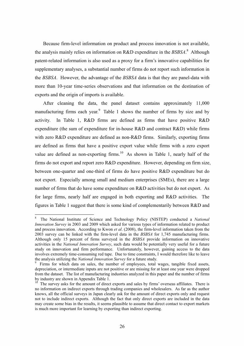
26  

Because firm-level information on product and process innovation is not available,

the analysis mainly relies on information on R&D expenditure in the BSBSA.8 Although

patent-related information is also used as a proxy for a firm’s innovative capabilities for

supplementary analyses, a substantial number of firms do not report such information in

the BSBSA. However, the advantage of the BSBSA data is that they are panel-data with

more than 10-year time-series observations and that information on the destination of

exports and the origin of imports is available.

After cleaning the data, the panel dataset contains approximately 11,000

manufacturing firms each year.9 Table 1 shows the number of firms by size and by

activity. In Table 1, R&D firms are defined as firms that have positive R&D

expenditure (the sum of expenditure for in-house R&D and contract R&D) while firms

with zero R&D expenditure are defined as non-R&D firms. Similarly, exporting firms

are defined as firms that have a positive export value while firms with a zero export

value are defined as non-exporting firms.10 As shown in Table 1, nearly half of the

firms do not export and report zero R&D expenditure. However, depending on firm size,

between one-quarter and one-third of firms do have positive R&D expenditure but do

not export. Especially among small and medium enterprises (SMEs), there are a large

number of firms that do have some expenditure on R&D activities but do not export. As

for large firms, nearly half are engaged in both exporting and R&D activities. The

figures in Table 1 suggest that there is some kind of complementarily between R&D and

                                                              8 The National Institute of Science and Technology Policy (NISTEP) conducted a National Innovation Survey in 2003 and 2009 which asked for various types of information related to product and process innovation. According to Kwon et al. (2008), the firm-level information taken from the 2003 survey can be linked with the firm-level data in the BSBSA for 1,745 manufacturing firms. Although only 15 percent of firms surveyed in the BSBSA provide information on innovative activities in the National Innovation Survey, such data would be potentially very useful for a future study on innovation and firm performance. Unfortunately, however, gaining access to the data involves extremely time-consuming red tape. Due to time constraints, I would therefore like to leave the analysis utilizing the National Innovation Survey for a future study. 9 Firms for which data on sales, the number of employees, total wages, tangible fixed assets, depreciation, or intermediate inputs are not positive or are missing for at least one year were dropped from the dataset. The list of manufacturing industries analyzed in this paper and the number of firms by industry are shown in Appendix Table 1. 10 The survey asks for the amount of direct exports and sales by firms’ overseas affiliates. There is no information on indirect exports through trading companies and wholesalers. As far as the author knows, all the official surveys in Japan clearly ask for the amount of direct exports only and request not to include indirect exports. Although the fact that only direct exports are included in the data may create some bias in the results, it seems plausible to assume that direct contact to export markets is much more important for learning by exporting than indirect exporting.

 

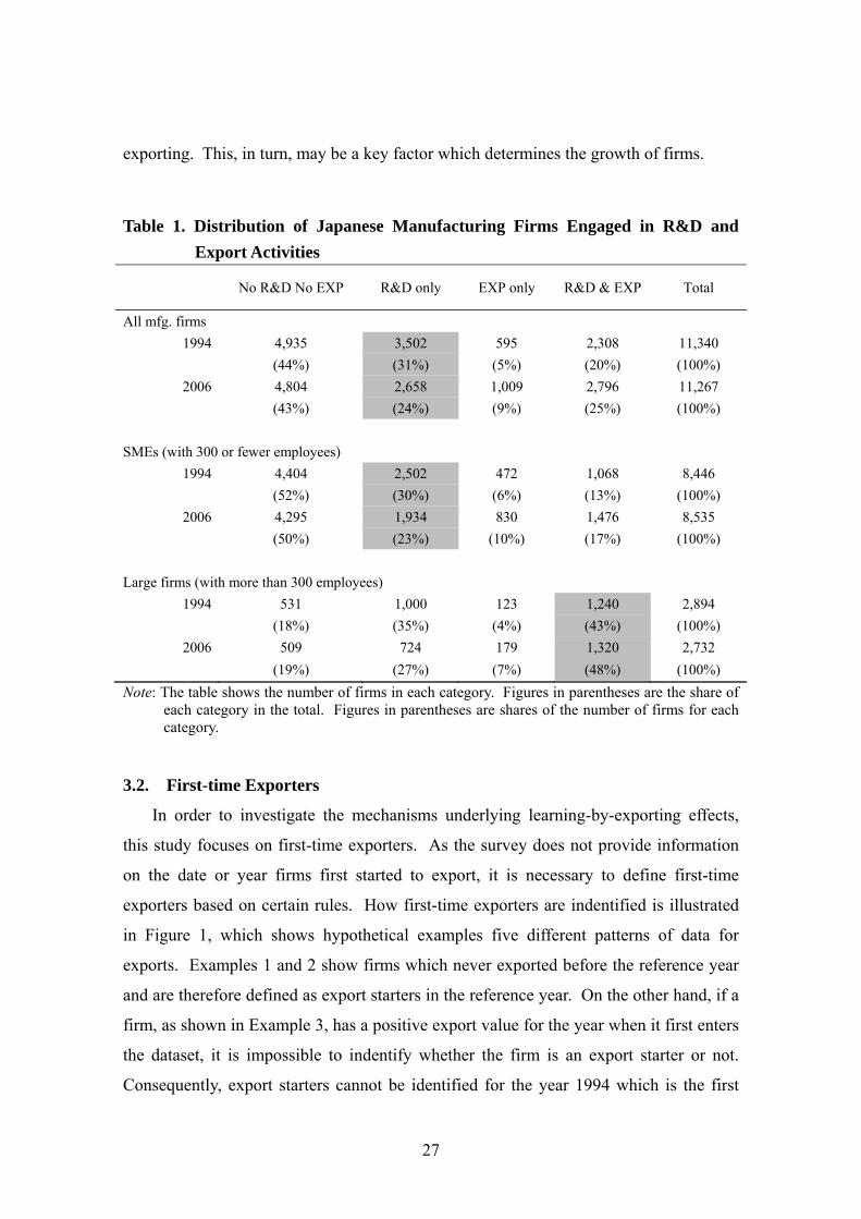
27  

exporting. This, in turn, may be a key factor which determines the growth of firms.

Table 1. Distribution of Japanese Manufacturing Firms Engaged in R&D and

Export Activities

No R&D No EXP R&D only EXP only R&D & EXP Total

All mfg. firms

1994 4,935 3,502 595 2,308 11,340

(44%) (31%) (5%) (20%) (100%)

2006 4,804 2,658 1,009 2,796 11,267

(43%) (24%) (9%) (25%) (100%)

SMEs (with 300 or fewer employees)

1994 4,404 2,502 472 1,068 8,446

(52%) (30%) (6%) (13%) (100%)

2006 4,295 1,934 830 1,476 8,535

(50%) (23%) (10%) (17%) (100%)

Large firms (with more than 300 employees)

1994 531 1,000 123 1,240 2,894

(18%) (35%) (4%) (43%) (100%)

2006 509 724 179 1,320 2,732

(19%) (27%) (7%) (48%) (100%)

Note: The table shows the number of firms in each category. Figures in parentheses are the share of each category in the total. Figures in parentheses are shares of the number of firms for each category.

3.2. First-time Exporters

In order to investigate the mechanisms underlying learning-by-exporting effects,

this study focuses on first-time exporters. As the survey does not provide information

on the date or year firms first started to export, it is necessary to define first-time

exporters based on certain rules. How first-time exporters are indentified is illustrated

in Figure 1, which shows hypothetical examples five different patterns of data for

exports. Examples 1 and 2 show firms which never exported before the reference year

and are therefore defined as export starters in the reference year. On the other hand, if a

firm, as shown in Example 3, has a positive export value for the year when it first enters

the dataset, it is impossible to indentify whether the firm is an export starter or not.

Consequently, export starters cannot be identified for the year 1994 which is the first

 

28  

year of the dataset, because the export status in the previous year is not available.

Moreover, it should be noted that there is a greater likelihood of misidentification of

export starters for early years in the dataset. Next, export quitters are similarly defined

as firms which stopped exporting and subsequently did not start exporting again

(Examples 1 and 3). If a firm has a positive export value for the last year in which it

appears in the dataset, it is impossible to indentify whether the firm is an export quitter

or not (Example 2). The definition of export quitters here also means that export

quitters cannot be identified for the year 2006, which is the last year of the dataset. It

should also be noted that there is a greater likelihood of misidentification of export

quitters for later years in the dataset. Moreover, some firms can be both export starters

and quitters (Example 1). Firms which have a positive export value for all years for

which observations for them are available in the dataset are defined as firms which

always export (Example 4), while firms which have a zero export value for all years for

which observations for them are available in the dataset are defined as firms which

never export (Example 5).

Figure 1. Examples for Export Starters and Quitters

Exports Exports Exports Exports Exports (ex.1) (ex.2) (ex.3) (ex.4) (ex.5)

1994 0 1 n.a. n.a. 1995 0 0 n.a. n.a. 1996 0 0 1 ALWAYS n.a. 1997 1 STARTER 1 1 0 NEVER 1998 0 0 1 0 1999 1 0 1 1 0 2000 0 0 0 1 0 2001 1 0 1 QUITTER 1 0 2002 1 QUITTER 1 STARTER 0 1 0 2003 0 1 0 1 0 2004 0 1 n.a. 1 0 2005 0 n.a. n.a. 1 n.a. 2006 0 n.a. n.a. 1 n.a.

Notes: 1: A positive export value; 0: A zero export value; n.a.: No observation in the dataset.

Table 2 summarizes the number of firms by export status over the period 1995-2005

by industry. The table shows that of the firms in the dataset, 2,408 newly entered export

markets during the period 1995-2005. At the same time, a significant number of firms

(1,636 firms) stopped exporting and did not start exporting again. In fact, 787 starter

 

29  

firms are also defined as quitters, suggesting that a significant number of export starters

quit exporting later.

Table 2. Number of Firms by Industry and by Export Status

STARTER QUITTER ALWAYS NEVER Industry total

No. % No. % No. % No. % No. %

1 Food products and beverages 159 (6.6) 153 (9.4) 88 (2.5) 2,243 (17.4) 2,601 (12.8)

2 Textiles 116 (4.8) 87 (5.3) 87 (2.4) 950 (7.3) 1,207 (6.0)

3 Lumber and wood products 41 (1.7) 34 (2.1) 22 (0.6) 505 (3.9) 589 (2.9)

4 Pulp, paper and paper products 66 (2.7) 43 (2.6) 29 (0.8) 500 (3.9) 623 (3.1)

5 Printing 43 (1.8) 31 (1.9) 25 (0.7) 804 (6.2) 890 (4.4)

6 Chemicals and chemical fibers 80 (3.3) 45 (2.8) 150 (4.2) 235 (1.8) 509 (2.5)

7 Paint, coating, and grease 30 (1.2) 33 (2.0) 60 (1.7) 75 (0.6) 196 (1.0)

8 Pharmaceutical products 35 (1.5) 29 (1.8) 84 (2.3) 139 (1.1) 291 (1.4)

9 Miscellaneous chemical products 68 (2.8) 49 (3.0) 145 (4.0) 133 (1.0) 391 (1.9)

10 Petroleum and coal products 12 (0.5) 10 (0.6) 20 (0.6) 35 (0.3) 75 (0.4)

11 Plastic products 154 (6.4) 89 (5.4) 137 (3.8) 664 (5.1) 1,023 (5.0)

12 Rubber products 24 (1.0) 18 (1.1) 56 (1.6) 115 (0.9) 213 (1.1)

13 Ceramic, stone and clay products 69 (2.9) 56 (3.4) 107 (3.0) 713 (5.5) 935 (4.6)

14 Iron and steel 89 (3.7) 81 (5.0) 60 (1.7) 411 (3.2) 605 (3.0)

15 Non-ferrous metals 79 (3.3) 52 (3.2) 103 (2.9) 232 (1.8) 460 (2.3)

16 Fabricated metal products 179 (7.4) 114 (7.0) 185 (5.2) 1,002 (7.8) 1,452 (7.2)

17 Metal processing machinery 59 (2.5) 46 (2.8) 137 (3.8) 140 (1.1) 376 (1.9)

18 Special industry machinery 78 (3.2) 58 (3.5) 208 (5.8) 252 (1.9) 612 (3.0)

19 Office and service industry machines 44 (1.8) 26 (1.6) 52 (1.5) 137 (1.1) 251 (1.2)

20 Miscellaneous machinery 179 (7.4) 120 (7.3) 335 (9.3) 479 (3.7) 1,104 (5.4)

21 Electrical machinery and apparatus 84 (3.5) 47 (2.9) 114 (3.2) 355 (2.7) 598 (2.9)

22 Household electric appliances 37 (1.5) 22 (1.3) 63 (1.8) 181 (1.4) 293 (1.4)

23 Communication equipment 52 (2.2) 44 (2.7) 98 (2.7) 225 (1.7) 409 (2.0)

24 Computer and electronic equipment 52 (2.2) 27 (1.7) 101 (2.8) 152 (1.2) 328 (1.6)

25 Electronic parts and devices 160 (6.6) 77 (4.7) 286 (8.0) 529 (4.1) 1,049 (5.2)

26 Miscellaneous electrical machinery 40 (1.7) 22 (1.3) 109 (3.0) 153 (1.2) 324 (1.6)

27 Motor vehicles and parts 211 (8.8) 93 (5.7) 217 (6.1) 795 (6.2) 1,286 (6.3)

28 Other transportation equipment 32 (1.3) 27 (1.7) 73 (2.0) 212 (1.6) 343 (1.7)

29 Precision machinery 75 (3.1) 46 (2.8) 257 (7.2) 191 (1.5) 581 (2.9)

30 Miscellaneous mfg. industries 61 (2.5) 57 (3.5) 175 (4.9) 369 (2.9) 659 (3.3)

1-30 Manufacturing Total 2,408 (100.0) 1,636 (100.0) 3,583 (100.0) 12,926 (100.0) 20,273 (100.0)

Notes: Firms are classified based on the industry reported for the first observation of each firm during the observation period. ALWAYS denotes firms which always exported throughout the sample period while NEVER denotes firms which never exported throughout

Table 3 shows a breakdown of export starters by firm characteristics.11 It indicates

that 74 percent of the 2,408 export starters are SMEs (firms with 300 or fewer

employees). This share more or less corresponds to the share of SMEs in the total

                                                              11 The number of export starters by year and the number of export quitters by year are shown in Appendix Table 2.

 

30  

number of firms in the dataset overall, which is 76 percent. Moreover, as expected, the

major export destination for both SMEs and larger firms is Asia.

Table 3. Number of Export Starters by Characteristics (Period Total)

Total SMEs Large firms

Export Starters 2,408 (100%) 1,780 (74%) 628 (26%)

Breakdown by Export Destination

Destinations Total 3,142 (100%) 2174 (100%) 968 (100%)

Asia 1,952 (62%) 1446 (67%) 506 (52%)

Middle East 64 (2%) 33 (2%) 31 (3%)

Europe 256 (8%) 165 (8%) 91 (9%)

North America 617 (20%) 395 (18%) 222 (23%)

Latin America 85 (3%) 50 (2%) 35 (4%)

Africa 47 (1%) 23 (1%) 24 (2%)

Oceania 121 (4%) 62 (3%) 59 (6%)

4. Econometric Analysis

4.1. Propensity Score Matching and DID Estimator

This section explains the econometric strategy employed to investigate the effects

of starting to export. Taking account of endogeneity among firms’ various strategies

and outcomes, propensity score matching is used to examine various outcomes of

starting exporting.

First, using logit estimation, the probability of initiating exporting for firms is

estimated and then a “propensity score” for each firm calculated. The propensity score

is defined as the conditional probability of initiating exporting given a firm’s

characteristics prior to exporting:

P x Pr z 1|x E z|x (1)

where z={0,1} indicates whether the firm started exporting in year t, and x is a vector of

observed firm characteristics in year t-1, i.e., the year prior to starting to export. For x,

the productivity level, firm size (proxied by the number of employees), R&D intensity

 

31  

(R&D expenditure divided by sales), age, the debt-asset ratio, the import-sales ratio, and

the FDI ratio (foreign investment divided by assets) are considered. 12 The main

productivity measure used here is total factor productivity (TFP) estimated using the

Olley-Pakes method. The production function is estimated by industry and the

estimated production function coefficients are shown in Appendix Table 3.13

Second, after estimating the logit model, firms which did not start exporting in year

t are matched with firms that had the closest propensity score and that actually did

initiate exporting. The matching is conducted separately for each year and industry.

Finally, the causal effect of initiating exporting on various performance variables is

examined. As shown in Rosenbaum and Rubin (1983), if the recipient of the treatment

(z in equation 1) is randomly chosen within cells defined by x in equation 1, it is also

randomly chosen within cells defined by the values of the single-index variable P(x).

Therefore, the Average effect of Treatment on the Treated (ATT) can be estimated as the

average difference between the outcome of recipients and non-recipients of the

treatment for which propensity scores P(x) are identical. In this case, the treatment is

the start of exporting. The propensity score matching technique should identify

matched firms that satisfy the assumption that, conditional on observables, the non-

treated outcomes are independent of the treatment status. Nonetheless, the propensity

score is conditional only on a limited number of observable characteristics, implying

that unobservable, time-invariant, firm-specific effects may not be fully removed after

propensity score matching. Therefore, the growth rate of the performance variables of

exporting firms, which is called the difference-in-differences (DID) estimator, is

compared between treated and non-treated firms. In this manner, these unobservable

effects can be reduced and more robust estimates can be obtained. The DID estimator

can be calculated as follows:

ATT DID ∑ y y ∑ y y (2)

                                                              12 Foreign investment here is defined as the amount of investment and/or lending to related firms (either subsidiaries and affiliates of the firm or those of the parent firm) located abroad. 13 The estimated coefficient of capital input was negative or insignificant in some cases. Therefore, the production function was estimated at a more aggregated industry level. However, there are still some cases where the coefficient of capital input was not statistically significant.

 

32  

where n denotes the number of observations and y denotes performance variables. For y,

productivity (TFP), demand (firm sales), R&D intensity, R&D volume (R&D

expenditure and employees in R&D divisions), firm size (employment and capital

stock), and skill intensity (R&D employment share) are considered. It is then examined

how and whether exporting changes these performance measures.

4.2. Matching Results

In order to examine the determinants of export initiation, observations of firms

which did not export before and started exporting for the first time during the sample

period are used. Observations of firms which exported throughout and firms which

exported but quit exporting before the reference year are excluded. The result of the

logit estimation is shown in column (1) of Table 4 and indicates that larger (in terms of

employment), more R&D intensive, older, and financially healthier firms are more

likely to become exporters. Moreover, the significantly positive coefficients for the

import and FDI ratios suggest that having some sort of link with international markets is

a key determinant of starting to export. However, the coefficient on productivity is not

statistically significant, suggesting that the productivity level is not a relevant

determinant of starting to export.14 Based on the logit estimation, firms are matched

separately for each year and industry using the one-to-one nearest neighbor matching

method.15 The balancing property test results are shown in Panel (a) of Appendix Table

4.16 Table 5 shows the estimated effects of starting to export, with s denoting the year

after the treatment (s in equation 2 above). Table 5 suggests that firms that started

exporting show significantly higher sales and employment growth rates than firms that

did not start exporting (rows (d) and (l)). Moreover, starting to export promotes R&D

activities and increases the R&D intensity and R&D volume (rows (e) to (j) and rows

                                                              14 This result is not consistent with the theoretical prediction by Melitz (2003) and others that export starters should be more productive in order to cover the fixed costs involved in starting to export. However, results by Todo (2009) for Japan suggest that productivity has a positive impact on the export decision, although the impact is economically negligible in size. The insignificant coefficient on TFP in Table 4 seems consistent with Todo’s results. 15 The matching procedure is implemented in Stata11 using a modified version of the procedure provided by Leuven and Sianesi (2003). 16 The balancing property is not adequately satisfied for some cases in Appendix Table 4, though the specification provided the best results in terms of the balancing property tests out of the several specifications tried.

 

33  

(o) and (p)). The positive effects of exporting on R&D activities continue even four

years after the firm started exporting. However, exporting does not have a significantly

positive effect on productivity in most cases (rows (a) and (b)). It should be noted that

actually a significant number of treated and control firms are dropped from the sample

in later years and only surviving firms are included in the ATT and DID analyses.

Moreover, a substantial number of treated firms stopped exporting after they started

exporting. For some cases, treated firms are retained in the sample while the matched

control firms are dropped from the sample, or vice versa, in later years. As can be seen

in Table 5, the numbers of treated firms and control firms are not balanced in later years.

Because firms which are dropped from the sample or whose export status switches may

create some bias in the results, they are excluded when estimating the effects of starting

to export.17 The results are shown in Table 6 and are mostly consistent with those in

Table 5. For the estimation shown in Table 6, only treated firms which continued

exporting and whose control firms were not dropped from the sample are included.

However, as before (Table 5), starting to export has no (or at best a weakly significant)

positive effect on productivity.

Table 4. Determinants of Export Initiation

Logit Multinomial logit

(1) (2) (3) (4)

STARTER=1 NAEUR=3 ASIA=2 OTHERS=1

lnTFP (OP) -0.0472 0.2313 -0.1567 -0.6203

(0.1325) (0.2318) (0.1606) (0.6843)

ln(employment) 0.3879*** 0.5366*** 0.3152*** 0.3056**

(0.0263) (0.0422) (0.0331) (0.1284)

R&D intensity 10.7083*** 14.1406*** 8.0768*** 10.1582**

(1.0193) (1.3279) (1.3527) (4.0193)

Age 0.0026*** 0.0023* 0.0027*** 0.0025

(0.0007) (0.0014) (0.0008) (0.0048)

Debt-asset ratio -0.1744* -0.2806* -0.1134 -0.5149

(0.0892) (0.1608) (0.1056) (0.4708)

Import ratio 1.8835*** 1.5279*** 1.9775*** 2.5612***

(0.1705) (0.3218) (0.1937) (0.6432)

                                                              17 Specifically, a pair of firms is excluded when one of the pair is dropped from the sample or when the treated firm stopped exporting.

 

34  

Table 4 (continued). Determinants of Export Initiation

Logit Multinomial logit

(1) (2) (3) (4)

STARTER=1 NAEUR=3 ASIA=2 OTHERS=1

FDI ratio 8.6690*** 8.4402*** 8.8450*** 6.6518**

(0.6541) (1.0077) (0.7229) (2.6418)

No. of observations 69,912 69,912

Chi-squared 1735.51 1997.66

Pseudo R^2 0.0931 0.0916

Log likelihood -8450.0695 -9901.9601

Note: Standard errors are in parentheses, with ***, **, and * indicating significance at the 1%, 5%, and 10% levels, respectively. The constant term is not reported. All equations include three-digit industry dummy variables and year dummy variables.

Table 5. Estimated Effects of Starting to Export

S 0 1 2 3 4

No. of observations 4,136 3,528 3,165 2,792 2,448

Treated 2,068 1,748 1,581 1,413 1,243

Control 2,068 1,780 1,584 1,379 1,205

Outcome

(a) Productivity level (lnTFP_OP)

-0.0059 0.0011 -0.0069 -0.0022 0.0047

(0.0120) (0.0104) (0.0128) (0.0114) (0.0124)

(b) Productivity growth rate: pre-export level (s=-1)

0.0032 0.0109 * 0.0038 0.0062 0.0067

(0.0052) (0.0059) (0.0064) (0.0076) (0.0083)

(c) Sales (lnY)

-0.0512 -0.0234 -0.0302 -0.0207 -0.0278

(0.0401) (0.0393) (0.0488) (0.0517) (0.0487)

(d) Sales growth rate: pre-export level (s=-1)

0.0245 *** 0.0365 *** 0.0388 *** 0.0403 *** 0.0494 ***

(0.0073) (0.0091) (0.0119) (0.0142) (0.0177)

(e) R&D intensity

0.0010 0.0021 *** 0.0031 *** 0.0034 *** 0.0032 ***

(0.0007) (0.0008) (0.0008) (0.0009) (0.0010)

 

35  

Table 5 (continued). Estimated Effects of Starting to Export

S 0 1 2 3 4

(f) Difference in R&D intensity: pre-export level (s=-1)

0.0002 0.0015 *** 0.0022 *** 0.0026 *** 0.0019 **

(0.0006) (0.0005) (0.0007) (0.0007) (0.0008)

(g) R&D expenditure (lnR&D exp)

1.7512 *** 1.9901 *** 2.2229 *** 2.0099 *** 2.1944 ***

(0.3155) (0.2983) (0.3805) (0.3740) (0.3577)

(h) R&D expenditure growth rate: pre-export level (s=-1)

0.4626 *** 0.4845 ** 0.7079 *** 0.6213 ** 0.7254 **

(0.1689) (0.2184) (0.2328) (0.2736) (0.3075)

(i) R&D employment (lnR&D emp)

0.2383 *** 0.2548 *** 0.2819 *** 0.3128 *** 0.2978 ***

(0.0488) (0.0549) (0.0571) (0.0673) (0.0587)

(j) R&D employment growth rate: pre-export level (s=-1)

0.0883 *** 0.0844 *** 0.1026 *** 0.1299 *** 0.1358 **

(0.0245) (0.0283) (0.0370) (0.0388) (0.0536)

(k) Employment (ln employment)

-0.1104 *** -0.0915 ** -0.0910 *** -0.0830 ** -0.0932 **

(0.0247) (0.0335) (0.0321) (0.0362) (0.0372)

(l) Employment growth rate: pre-export level (s=-1)

0.0201 *** 0.0275 *** 0.0337 *** 0.0368 *** 0.0317 ***

(0.0043) (0.0057) (0.0072) (0.0093) (0.0106)

(m) Capital stock (ln K)

-0.0606 -0.0365 -0.0018 0.0042 -0.0083

(0.0514) (0.0429) (0.0521) (0.0554) (0.0562)

(n) Capital stock growth rate: pre-export level (s=-1)

0.0190 * 0.0202 0.0386 *** 0.0438 ** 0.0675 ***

(0.0111) (0.0125) (0.0139) (0.0190) (0.0234)

(o) R&D employment share

0.0113 *** 0.0131 *** 0.0134 *** 0.0165 *** 0.0145 ***

(0.0025) (0.0024) (0.0026) (0.0026) (0.0033)

(p) Difference in R&D employment share: pre-export level (s=-1)

0.0021 0.0030 * 0.0030 0.0058 *** 0.0047 **

(0.0015) (0.0018) (0.0018) (0.0021) (0.0024)

Notes: Bootstrapped standard errors are in parentheses (100 repetitions). ***, **, and * indicate significance at the 1%, 5%, and 10% levels, respectively.

 

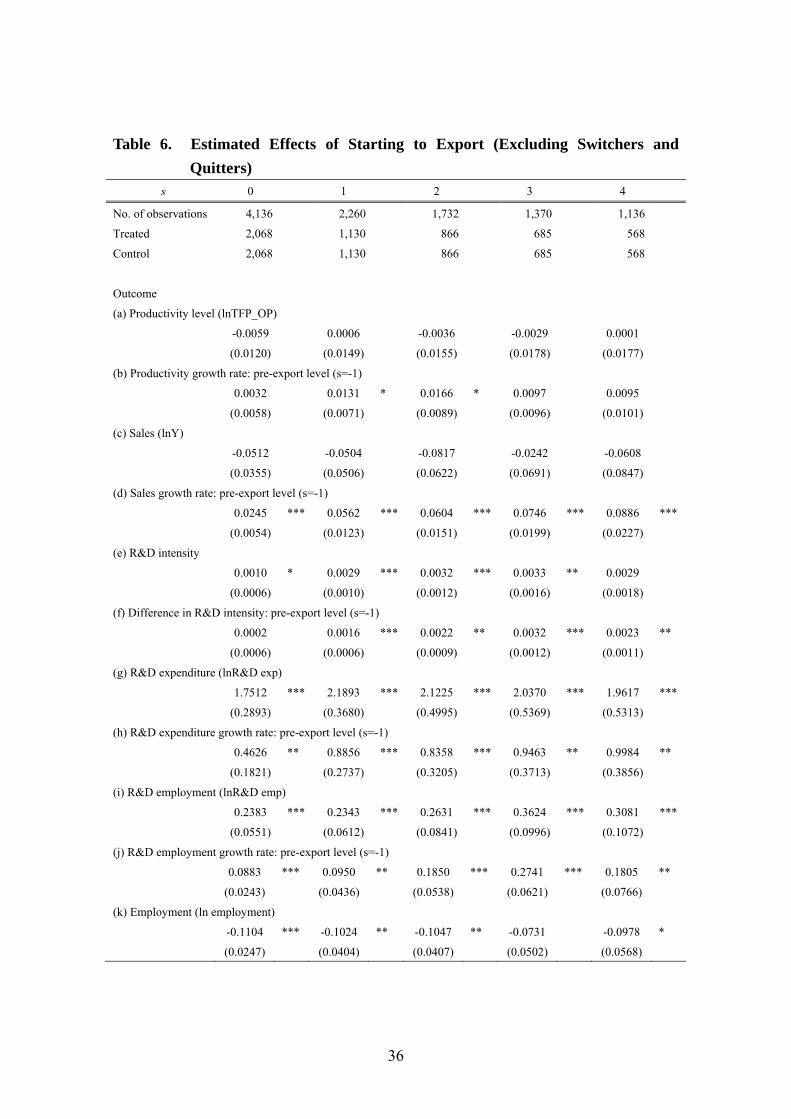
36  

Table 6. Estimated Effects of Starting to Export (Excluding Switchers and

Quitters) s 0 1 2 3 4

No. of observations 4,136 2,260 1,732 1,370 1,136

Treated 2,068 1,130 866 685 568

Control 2,068 1,130 866 685 568

Outcome

(a) Productivity level (lnTFP_OP)

-0.0059 0.0006 -0.0036 -0.0029 0.0001

(0.0120) (0.0149) (0.0155) (0.0178) (0.0177)

(b) Productivity growth rate: pre-export level (s=-1)

0.0032 0.0131 * 0.0166 * 0.0097 0.0095

(0.0058) (0.0071) (0.0089) (0.0096) (0.0101)

(c) Sales (lnY)

-0.0512 -0.0504 -0.0817 -0.0242 -0.0608

(0.0355) (0.0506) (0.0622) (0.0691) (0.0847)

(d) Sales growth rate: pre-export level (s=-1)

0.0245 *** 0.0562 *** 0.0604 *** 0.0746 *** 0.0886 ***

(0.0054) (0.0123) (0.0151) (0.0199) (0.0227)

(e) R&D intensity

0.0010 * 0.0029 *** 0.0032 *** 0.0033 ** 0.0029

(0.0006) (0.0010) (0.0012) (0.0016) (0.0018)

(f) Difference in R&D intensity: pre-export level (s=-1)

0.0002 0.0016 *** 0.0022 ** 0.0032 *** 0.0023 **

(0.0006) (0.0006) (0.0009) (0.0012) (0.0011)

(g) R&D expenditure (lnR&D exp)

1.7512 *** 2.1893 *** 2.1225 *** 2.0370 *** 1.9617 ***

(0.2893) (0.3680) (0.4995) (0.5369) (0.5313)

(h) R&D expenditure growth rate: pre-export level (s=-1)

0.4626 ** 0.8856 *** 0.8358 *** 0.9463 ** 0.9984 **

(0.1821) (0.2737) (0.3205) (0.3713) (0.3856)

(i) R&D employment (lnR&D emp)

0.2383 *** 0.2343 *** 0.2631 *** 0.3624 *** 0.3081 ***

(0.0551) (0.0612) (0.0841) (0.0996) (0.1072)

(j) R&D employment growth rate: pre-export level (s=-1)

0.0883 *** 0.0950 ** 0.1850 *** 0.2741 *** 0.1805 **

(0.0243) (0.0436) (0.0538) (0.0621) (0.0766)

(k) Employment (ln employment)

-0.1104 *** -0.1024 ** -0.1047 ** -0.0731 -0.0978 *

(0.0247) (0.0404) (0.0407) (0.0502) (0.0568)

 

37  

Table 6 (continued). Estimated Effects of Starting to Export (Excluding Switchers

and Quitters) s 0 1 2 3 4

Notes: Bootstrapped standard errors are in parentheses (100 repetitions). ***, **, and * indicate significance at the 1%, 5%, and 10% levels, respectively.

4.3. Learning-by-Exporting Effects by Export Destination

In order to further investigate the mechanism of learning-by-exporting, the sample

is split according to the destination market and the effect of exporting is estimated

separately for firms exporting to high-income regions and low-income regions.

Conducting such estimations by region, it is then examined whether the effects of

exporting differ across export destinations. Because the survey only asks respondents to

name the export region, such as Asia, North America, and Europe, the following four

cases are distinguished: (1) firms which do not export; (2) firms which do not export to

Asia, North America, or Europe, but do export to other regions; (3) firms which do not

export to North America or Europe, but do export to Asia (and other regions); and (4)

firms exporting to North America or Europe (and Asia and/or other regions). That is,

for example, if a firm exports to both North America and Asia in the initial year of

exporting, the firm is classified as falling into the fourth category. Similarly, if a firm

exports to both Asia and Oceania in the initial year of exporting, the firm is classified as

falling into the third category. And if a firm exports to Europe only, the firm is

(l) Employment growth rate: pre-export level (s=-1)

0.0201 *** 0.0340 *** 0.0412 *** 0.0573 *** 0.0573 ***

(0.0043) (0.0078) (0.0107) (0.0130) (0.0172)

(m) Capital stock (ln K)

-0.0606 -0.0655 -0.0952 -0.0304 -0.0968

(0.0514) (0.0720) (0.0732) (0.0812) (0.0844)

(n) Capital stock growth rate: pre-export level (s=-1)

0.0190 * 0.0156 0.0290 0.0068 0.0447

(0.0111) (0.0171) (0.0212) (0.0272) (0.0300)

(o) R&D employment share

0.0113 *** 0.0125 *** 0.0135 *** 0.0174 *** 0.0141 ***

(0.0025) (0.0038) (0.0043) (0.0042) (0.0051)

(p) Difference in R&D employment share: pre-export level (s=-1)

0.0021 0.0025 0.0056 ** 0.0098 *** 0.0038

(0.0015) (0.0023) (0.0026) (0.0030) (0.0038)

 

38  

classified as falling into the fourth category.18 In order to estimate the determinants of

exporting for each category of firms, equation (1) is modified into a multinomial logit

model. The indicator of initiating exporting in year t, z, now takes a value of 0, 1, 2, or

3, corresponding to the four cases. The multinomial logit estimation results are shown

in columns (2) to (4) of Table 4.19 Based on the multinomial logit estimation, firms are

matched separately for each year and industry using the one-to-one nearest neighbor

matching method. The balancing property test results are shown in Panels (b) to (d) of

Appendix Table 4.

Tables 7 to 9 show the estimated effects of starting to export. The results in Table 7

suggest that starting to export to North America or Europe has a strong positive effect

on sales and employment growth and R&D activities. Moreover, exporting to these

regions improves the productivity growth rate significantly. However, starting to export

to Asia does not have any productivity enhancing effects, although it tends to raise the

growth rate of sales and increase R&D expenditure (Table 8). Starting to export to other

regions has almost no significant effect, though the results may be due to the small

sample size (Table 9).

Table 7. Estimated Effects of Starting to Export to North America or Europe

S 0 1 2 3 4

No. of observations 1,260 1,096 967 859 764

Treated 630 551 498 445 389

Control 630 545 469 414 375

Outcome

(a) Productivity level (lnTFP_OP)

0.0116 0.0275 0.0002 -0.0008 0.0066

(0.0205) (0.0215) (0.0187) (0.0233) (0.0255)

(b) Productivity growth rate: pre-export level (s=-1)

0.0163 ** 0.0293 *** 0.0183 0.0182 0.0153

(0.0079) (0.0104) (0.0127) (0.0134) (0.0149)

                                                              18 The number of firms for each category is shown in Appendix Table 5. 19 The results in columns (2) to (4) of Table 4 are similar to that in column (1). However, size (as measured by employment) and R&D intensity have a larger impact on the decision to export to North America/Europe than on decision to export to Asia and other regions. As for the productivity level, although the estimated coefficients are not statistically significant, a positive coefficient is estimated only in the case of the decision to export to North America/Europe, suggesting that productivity is a more important determinant for export starters to developed regions than for those to developing regions.

 

39  

Table 7 (continued). Estimated Effects of Starting to Export to North America or

Europe S 0 1 2 3 4

(c) Sales (lnY)

0.0735 0.0895 0.0818 0.0997 0.1299

(0.0787) (0.0704) (0.0854) (0.0874) (0.0946)

(d) Sales growth rate: pre-export level (s=-1)

0.0672 *** 0.0791 *** 0.0893 *** 0.0787 ** 0.0924 ***

(0.0140) (0.0162) (0.0214) (0.0239) (0.0323)

(e) R&D intensity

0.0026 0.0041 ** 0.0057 *** 0.0069 *** 0.0070 ***

(0.0019) (0.0020) (0.0018) (0.0024) (0.0022)

(f) Difference in R&D intensity: pre-export level (s=-1)

-0.0007 0.0012 0.0021 0.0034 ** 0.0020

(0.0012) (0.0012) (0.0015) (0.0016) (0.0014)

(g) R&D expenditure (lnR&D exp)

3.4182 *** 3.4800 *** 3.7098 *** 3.8470 *** 3.9876 ***

(0.4810) (0.5550) (0.6499) (0.6505) (0.6974)

(h) R&D expenditure growth rate: pre-export level (s=-1)

0.6047 * 0.5624 0.8818 * 1.2263 ** 1.0353 *

(0.3437) (0.4300) (0.5251) (0.5752) (0.5609)

(i) R&D employment (lnR&D emp)

0.3489 *** 0.3903 *** 0.4981 *** 0.5052 *** 0.4992 ***

(0.0903) (0.1113) (0.1187) (0.1138) (0.1204)

(j) R&D employment growth rate: pre-export level (s=-1)

0.0478 0.0588 0.1934 *** 0.2272 *** 0.1882 *

(0.0542) (0.0661) (0.0726) (0.0810) (0.0992)

(k) Employment (ln employment)

-0.0250 -0.0121 -0.0348 -0.0131 0.0000

(0.0567) (0.0641) (0.0618) (0.0717) (0.0813)

(l) Employment growth rate: pre-export level (s=-1)

0.0364 *** 0.0528 *** 0.0470 *** 0.0517 *** 0.0458 **

(0.0087) (0.0116) (0.0158) (0.0184) (0.0210)

(m) Capital stock (ln K)

0.1298 0.1178 0.0884 0.1190 0.1391

(0.0794) (0.0851) (0.1033) (0.1162) (0.1140)

(n) Capital stock growth rate: pre-export level (s=-1)

0.0393 0.0351 0.0399 0.0508 0.0997 **

(0.0257) (0.0228) (0.0367) (0.0398) (0.0449)

(o) R&D employment share

0.0177 *** 0.0178 *** 0.0210 *** 0.0218 *** 0.0219 ***

(0.0052) (0.0057) (0.0051) (0.0057) (0.0071)

 

40  

Table 7 (continued). Estimated Effects of Starting to Export to North America or

Europe S 0 1 2 3 4

(p) Difference in R&D employment share: pre-export level (s=-1)

0.0005 -0.0001 0.0035 0.0062 0.0046

(0.0030) (0.0032) (0.0037) (0.0046) (0.0053)

Notes: Bootstrapped standard errors are in parentheses (100 repetitions). ***, **, and * indicate significance at the 1%, 5%, and 10% levels, respectively.

Table 8. Estimated Effects of Starting to Export to Asia s 0 1 2 3 4

No. of observations 2,714 2,283 2,049 1,787 1,565

Treated 1,357 1,129 1,019 909 798

Control 1,357 1,154 1,030 878 767

Outcome

(a) Productivity level (lnTFP_OP)

-0.0076 -0.0062 -0.0050 -0.0111 -0.0055

(0.0130) (0.0141) (0.0143) (0.0154) (0.0169)

(b) Productivity growth rate: pre-export level (s=-1)

-0.0058 -0.0018 -0.0057 -0.0124 -0.0116

(0.0060) (0.0081) (0.0085) (0.0089) (0.0101)

(c) Sales (lnY)

-0.0840 ** -0.0831 -0.1021 * -0.0798 -0.1001 *

(0.0403) (0.0507) (0.0536) (0.0530) (0.0553)

(d) Sales growth rate: pre-export level (s=-1)

0.0101 0.0165 0.0215 0.0214 0.0146

(0.0072) (0.0106) (0.0140) (0.0164) (0.0208)

(e) R&D intensity

-0.0001 0.0010 0.0018 ** 0.0018 ** 0.0020 **

(0.0007) (0.0008) (0.0009) (0.0009) (0.0010)

(f) Difference in R&D intensity: pre-export level (s=-1)

0.0010 ** 0.0020 *** 0.0028 *** 0.0027 *** 0.0029 ***

(0.0005) (0.0005) (0.0006) (0.0007) (0.0008)

(g) R&D expenditure (lnR&D exp)

0.8434 ** 1.0986 *** 1.3299 *** 0.9912 *** 1.6074 ***

(0.3728) (0.3999) (0.4311) (0.3591) (0.4775)

(h) R&D expenditure growth rate: pre-export level (s=-1)

0.2539 0.2348 0.6511 ** 0.3137 0.7421 **

(0.2316) (0.2913) (0.2992) (0.3488) (0.3660)

 

41  

Table 8 (continued). Estimated Effects of Starting to Export to Asia s 0 1 2 3 4

(i) R&D employment (lnR&D emp)

0.0883 0.1212 * 0.1376 ** 0.1334 * 0.1574 *

(0.0595) (0.0681) (0.0569) (0.0700) (0.0893)

(j) R&D employment growth rate: pre-export level (s=-1)

0.0414 0.0567 * 0.1041 ** 0.0808 0.0924 *

(0.0336) (0.0321) (0.0436) (0.0561) (0.0552)

(k) Employment (ln employment)

-0.1389 *** -0.1446 *** -0.1327 *** -0.1398 *** -0.1484 ***

(0.0320) (0.0355) (0.0361) (0.0404) (0.0439)

(l) Employment growth rate: pre-export level (s=-1)

0.0113 ** 0.0094 0.0210 ** 0.0127 0.0050

(0.0051) (0.0066) (0.0095) (0.0125) (0.0159)

(m) Capital stock (ln K)

-0.1244 ** -0.1105 * -0.1102 ** -0.0819 -0.0892

(0.0525) (0.0640) (0.0518) (0.0641) (0.0756)

(n) Capital stock growth rate: pre-export level (s=-1)

0.0113 0.0079 0.0273 0.0350 0.0495 *

(0.0125) (0.0146) (0.0184) (0.0216) (0.0272)

(o) R&D employment share

0.0072 *** 0.0072 *** 0.0088 *** 0.0101 *** 0.0097 ***

(0.0022) (0.0027) (0.0028) (0.0030) (0.0033)

(p) Difference in R&D employment share: pre-export level (s=-1)

0.0014 0.0006 0.0030 0.0029 0.0030

(0.0015) (0.0022) (0.0022) (0.0027) (0.0026)

Notes: Bootstrapped standard errors are in parentheses (100 repetitions). ***, **, and * indicate significance at the 1%, 5%, and 10% levels, respectively.

Table 9. Estimated Effects of Starting to Export to Other Regions s 0 1 2 3 4

No. of observations 162 139 126 116 108

Treated 81 68 64 59 56

Control 81 71 62 57 52

Outcome

(a) Productivity level (lnTFP_OP)

0.0012 -0.0034 -0.0592 -0.0399 -0.0133

(0.0629) (0.0599) (0.0627) (0.0646) (0.0639)

(b) Productivity growth rate: pre-export level (s=-1)

-0.0016 0.0109 -0.0037 0.0063 0.0181

(0.0288) (0.0261) (0.0283) (0.0324) (0.0308)

 

42  

Table 9 (continued). Estimated Effects of Starting to Export to Other Regions s 0 1 2 3 4

(c) Sales (lnY)

-0.1661 -0.1221 -0.2292 -0.1309 -0.2771

(0.2107) (0.2405) (0.2271) (0.2733) (0.2617)

(d) Sales growth rate: pre-export level (s=-1)

0.0235 0.0211 0.0220 0.0460 0.0439

(0.0257) (0.0455) (0.0472) (0.0738) (0.0854)

(e) R&D intensity

-0.0022 -0.0003 0.0004 -0.0014 0.0004

(0.0024) (0.0036) (0.0023) (0.0034) (0.0042)

(f) Difference in R&D intensity: pre-export level (s=-1)

-0.0035 ** 0.0001 -0.0017 -0.0038 -0.0026

(0.0017) (0.0026) (0.0020) (0.0032) (0.0027)

(g) R&D expenditure (lnR&D exp)

0.9664 -0.1326 1.5564 0.1427 -0.0091

(1.2480) (1.6405) (1.8298) (1.7239) (1.7060)

(h) R&D expenditure growth rate: pre-export level (s=-1)

0.1393 -0.9247 -0.4689 -2.5038 ** -2.4948 **

(0.7628) (0.8846) (1.1400) (1.3289) (1.1326)

(i) R&D employment (lnR&D emp)

-0.1133 -0.4866 * -0.1372 -0.0372 -0.1834

(0.2434) (0.2795) (0.2609) (0.3065) (0.3284)

(j) R&D employment growth rate: pre-export level (s=-1)

0.2290 * -0.1179 0.1023 0.0965 -0.0437

(0.1364) (0.1875) (0.1954) (0.2267) (0.1722)

(k) Employment (ln employment)

-0.2544 -0.2602 -0.3662 ** -0.2869 -0.4188 **

(0.1639) (0.2021) (0.1821) (0.1776) (0.2014)

(l) Employment growth rate: pre-export level (s=-1)

0.0076 0.0011 0.0036 0.0035 -0.0174

(0.0173) (0.0238) (0.0317) (0.0511) (0.0512)

(m) Capital stock (ln K)

-0.1134 -0.0802 -0.1415 -0.0394 -0.1564

(0.2431) (0.2354) (0.3030) (0.2880) (0.3167)

(n) Capital stock growth rate: pre-export level (s=-1)

-0.0400 -0.0811 -0.0343 0.0515 0.0572

(0.0459) (0.0710) (0.0859) (0.0937) (0.0952)

(o) R&D employment share

0.0051 0.0001 0.0065 0.0167 0.0054

(0.0089) (0.0129) (0.0103) (0.0158) (0.0115)

(p) Difference in R&D employment share: pre-export level (s=-1)

0.0051 0.0015 0.0005 * 0.0110 -0.0032

(0.0057) (0.0106) (0.0084) (0.0155) (0.0065)

Notes: Bootstrapped standard errors are in parentheses (100 repetitions). ***, **, and * indicate significance at the 1%, 5%, and 10% levels, respectively.

 

43  

The results in Tables 7 to 9 are based on observations of firms that survived s years

after the treatment year regardless of whether the export status of the treated firm

changed and of whether one of the pair was dropped from the sample. Therefore,

similar to Table 6, Tables 10 to 12 show estimates when these firms are excluded and

only treated firms which continued exporting and whose control firms were not dropped

from the sample are included. The results are mostly consistent with those in Tables 7

to 9. However, the magnitude of the positive impact is much larger in Tables 10 to 12

than in Tables 7 to 9. The results in Tables 10 to 12 pick up the effects for firms which

were able to stay and survive in the export market, and these firms are likely to have

enjoyed greater learning effects. That is, the results in Tables 10 to 12 may include a

selection effect (better performing firms were able to stay in the export market).

Table 10. Estimated Effects of Starting to Export to North America or Europe

(Excluding Switchers and Quitters) s 0 1 2 3 4

No. of observations 1,260 802 600 494 410

Treated 630 401 300 247 205

Control 630 401 300 247 205

Outcome

(a) Productivity level (lnTFP_OP)

0.0116 0.0211 0.0217 0.0138 0.0325

(0.0209) (0.0223) (0.0260) (0.0265) (0.0330)

(b) Productivity growth rate: pre-export level (s=-1)

0.0163 * 0.0243 ** 0.0384 *** 0.0304 0.0414 *

(0.0095) (0.0119) (0.0136) (0.0195) (0.0232)

(c) Sales (lnY)

0.0735 0.1216 0.0970 0.1951 * 0.2185 *

(0.0819) (0.0975) (0.1086) (0.1154) (0.1180)

(d) Sales growth rate: pre-export level (s=-1)

0.0672 *** 0.0966 *** 0.1149 *** 0.1051 *** 0.1223 ***

(0.0128) (0.0203) (0.0236) (0.0329) (0.0396)

(e) R&D intensity

0.0026 0.0051 ** 0.0043 * 0.0033 0.0043

(0.0018) (0.0025) (0.0024) (0.0030) (0.0029)

(f) Difference in R&D intensity: pre-export level (s=-1)

-0.0007 0.0014 0.0023 0.0037 0.0040 **

(0.0012) (0.0013) (0.0019) (0.0023) (0.0020)

 

44  

Table 10 (continued). Estimated Effects of Starting to Export to North America or

Europe (Excluding Switchers and Quitters) s 0 1 2 3 4

(g) R&D expenditure (lnR&D exp)

3.4182 *** 3.8709 *** 3.7914 *** 3.7351 *** 4.2656 ***

(0.5000) (0.6523) (0.6731) (0.8356) (0.9044)

(h) R&D expenditure growth rate: pre-export level (s=-1)

0.6047 * 0.7230 * 0.9719 1.3370 ** 1.3970 *

(0.3268) (0.4258) (0.5905) (0.6193) (0.7834)

(i) R&D employment (lnR&D emp)

0.3489 *** 0.5129 *** 0.5793 *** 0.5916 *** 0.5461 ***

(0.0809) (0.1135) (0.1527) (0.1698) (0.1569)

(j) R&D employment growth rate: pre-export level (s=-1)

0.0478 0.1231 0.3092 *** 0.3813 *** 0.2527 *

(0.0556) (0.0852) (0.1077) (0.1018) (0.1320)

(k) Employment (ln employment)

-0.0250 0.0093 -0.0102 0.0529 0.0547

(0.0567) (0.0747) (0.0809) (0.0811) (0.0979)

(l) Employment growth rate: pre-export level (s=-1)

0.0364

***

0.0608 *** 0.0574 *** 0.0761 *** 0.0759 ***

(0.0087) (0.0127) (0.0204) (0.0274) (0.0280)

(m) Capital stock (ln K)

0.1298 0.0702 0.0335 0.1621 0.1644

(0.0794) (0.1193) (0.1172) (0.1206) (0.1564)

(n) Capital stock growth rate: pre-export level (s=-1)

0.0393 0.0245 0.0530 0.0569 0.0528

(0.0257) (0.0311) (0.0340) (0.0399) (0.0444)

(o) R&D employment share

0.0177

***

0.0227 *** 0.0210 *** 0.0202 ** 0.0163

(0.0052) (0.0073) (0.0078) (0.0083) (0.0107)

(p) Difference in R&D employment share: pre-export level (s=-1)

0.0005 0.0014 0.0043 0.0111 * 0.0026

(0.0030) (0.0038) (0.0053) (0.0058) (0.0068)

Notes: Bootstrapped standard errors are in parentheses (100 repetitions). ***, **, and * indicate significance at the 1%, 5%, and 10% levels, respectively.

 

45  

Table 11. Estimated Effects of Starting to Export to Asia (Excluding Switchers and

Quitters) s 0 1 2 3 4

No. of observations

2,714

1,426

1,068

804

688

Treated 1,357 713 534 402 344

Control 1,357 713 534 402 344

Outcome

(a) Productivity level (lnTFP_OP)

-0.0076 -0.0052 -0.0091 -0.0065 -0.0126

(0.0128) (0.0195) (0.0184) (0.0243) (0.0268)

(b) Productivity growth rate: pre-export level (s=-1)

-0.0058 -0.0052 -0.0145 -0.0166 -0.0104

(0.0065) (0.0105) (0.0111) (0.0136) (0.0139)

(c) Sales (lnY)

-0.0840 * -0.0705 -0.0642 -0.0524 -0.1845 **

(0.0441) (0.0679) (0.0715) (0.0848) (0.0934)

(d) Sales growth rate: pre-export level (s=-1)

0.0101 0.0316 ** 0.0480 ** 0.0645 ** 0.0746 ***

(0.0068) (0.0129) (0.0188) (0.0258) (0.0277)

(e) R&D intensity

-0.0001 0.0009 0.0020 * 0.0017 0.0008

(0.0008) (0.0011) (0.0012) (0.0017) (0.0016)

(f) Difference in R&D intensity: pre-export level (s=-1)

0.0010 * 0.0020 *** 0.0033 *** 0.0035 *** 0.0038 ***

(0.0005) (0.0007) (0.0010) (0.0011) (0.0012)

(g) R&D expenditure (lnR&D exp)

0.8434 *** 0.8088 * 1.3798 ** 1.0851 * 0.9615

(0.3230) (0.4490) (0.5966) (0.6432) (0.6581)

(h) R&D expenditure growth rate: pre-export level (s=-1)

0.2539 0.4137 0.8632 ** 0.7703 1.3218 **

(0.2365) (0.3374) (0.3770) (0.4711) (0.5192)

(i) R&D employment (lnR&D emp)

0.0883 0.0742 0.1203 0.1439 -0.0008

(0.0591) (0.0771) (0.1028) (0.1193) (0.1182)

(j) R&D employment growth rate: pre-export level (s=-1)

0.0414 0.0500 0.1736 *** 0.1561 * 0.1251

(0.0266) (0.0479) (0.0562) (0.0852) (0.0958)

(k) Employment (ln employment)

-0.1389 *** -0.1202 ** -0.1030 * -0.1070 -0.2081 ***

(0.0320) (0.0505) (0.0603) (0.0670) (0.0694)

 

46  

Table 11 (continued). Estimated Effects of Starting to Export to Asia (Excluding

Switchers and Quitters) s 0 1 2 3 4

(l) Employment growth rate: pre-export level (s=-1)

0.0113 ** 0.0185 ** 0.0270 ** 0.0425 ** 0.0235

(0.0051) (0.0080) (0.0127) (0.0184) (0.0231)

(m) Capital stock (ln K)

-0.1244 ** -0.0754 -0.0978 -0.0314 -0.1963 *

(0.0525) (0.0776) (0.0843) (0.0876) (0.1069)

(n) Capital stock growth rate: pre-export level (s=-1)

0.0113 0.0329 * 0.0394 * 0.0370 0.0607

(0.0125) (0.0185) (0.0236) (0.0289) (0.0398)

(o) R&D employment share

0.0072 *** 0.0051 0.0081 * 0.0091 * 0.0034

(0.0022) (0.0036) (0.0047) (0.0054) (0.0059)

(p) Difference in R&D employment share: pre-export level (s=-1)

0.0014 -0.0011 0.0070 ** 0.0050 0.0014

(0.0015) (0.0025) (0.0031) (0.0042) (0.0037)

Notes: Bootstrapped standard errors are in parentheses (100 repetitions). ***, **, and * indicate significance at the 1%, 5%, and 10% levels, respectively.

Table 12. Estimated Effects of Starting to Export to Other Regions (Excluding

Switchers and Quitters)

s 0 1 2 3 4

No. of observations 162 46 34 46 38

Treated 81 23 17 23 19

Control 81 23 17 23 19

Outcome

(a) Productivity level (lnTFP_OP)

0.0012 0.0163 -0.0272 0.0232 0.0211

(0.0594) (0.1139) (0.1055) (0.0935) (0.0786)

(b) Productivity growth rate: pre-export level (s=-1)

-0.0016 0.0135 0.0021 0.0374 0.0053

(0.0329) (0.0489) (0.0466) (0.0297) (0.0460)

(c) Sales (lnY)

-0.1661 -0.3473 -0.1230 0.0050 -0.2152

(0.1977) (0.4122) (0.4522) (0.4389) (0.4567)

(d) Sales growth rate: pre-export level (s=-1)

0.0235 -0.0252 0.0810 0.2824 ** 0.2364 *

(0.0242) (0.0577) (0.0763) (0.1275) (0.1349)

 

47  

Table 12 (continued). Estimated Effects of Starting to Export to Other Regions

(Excluding Switchers and Quitters)

(j) R&D employment growth rate: pre-export level (s=-1)

0.2290 0.2214 0.2816 0.6055 * -0.0702

(0.1448) (0.2901) (0.2791) (0.3094) (0.3296)

(k) Employment (ln employment)

-0.2544 -0.2539 -0.3234 -0.2386 -0.3643

(0.1639) (0.3291) (0.3419) (0.3743) (0.3839)

(l) Employment growth rate: pre-export level (s=-1)

0.0076 -0.0052 0.0270 0.1423 * 0.0992

(0.0173) (0.0383) (0.0545) (0.0744) (0.1123)

(m) Capital stock (ln K)

-0.1134 -0.1511 0.1499 0.0175 -0.2705

(0.2431) (0.4549) (0.5165) (0.4938) (0.5603)

(n) Capital stock growth rate: pre-export level (s=-1)

-0.0400 -0.3158 -0.0712 -0.0421 0.0574

(0.0459) (0.1339) (0.1682) (0.1548) (0.1689)

(o) R&D employment share

0.0051 0.0245 0.0260 0.0439 0.0234

(0.0089) (0.0334) (0.0204) (0.0370) (0.0253)

(p) Difference in R&D employment share: pre-export level (s=-1)

0.0051 0.0199 0.0146 0.0309 -0.0182

(0.0057) (0.0248) (0.0102) (0.0290) (0.0170)

Notes: Bootstrapped standard errors are in parentheses (100 repetitions). ***, **, and * indicate significance at the 1%, 5%, and 10% levels, respectively.

s 0 1 2 3 4

(e) R&D intensity

-0.0022 0.0054 -0.0009 -0.0041 0.0086

(0.0025) (0.0086) (0.0041) (0.0072) (0.0082)

(f) Difference in R&D intensity: pre-export level (s=-1)

-0.0035 * 0.0035 -0.0027 -0.0080 -0.0018

(0.0019) (0.0068) (0.0029) (0.0062) (0.0058)

(g) R&D expenditure (lnR&D exp)

0.9664 2.3205 2.9209 4.0153 4.4645

(1.4966) (2.5162) (2.7583) (3.2764) (2.8545)

(h) R&D expenditure growth rate: pre-export level (s=-1)

0.1393 -0.4879 -2.7956 -2.4023 -2.6873

(0.7929) (2.0349) (2.2592) (2.4439) (1.7564)

(i) R&D employment (lnR&D emp)

-0.1133 -0.0994 0.0826 0.7269 0.3655

(0.2487) (0.5277) (0.3983) (0.4602) (0.5408)

 

48  

However, the results in Tables 10 to 12 confirm that starting to export to North

America/Europe has a larger positive effect on the growth rates of productivity, sales,

R&D activity, and employment than starting to export to Asia. Table 13 provides a

summary of the differences in the impact two and four years after starting to export to

North America/Europe and to Asia. Specifically, the Table shows the difference in the

growth rate of various performance indicators of export starters vis-à-vis firms with the

closest propensity score that did not export. The figures clearly indicate that starting to

export to North America/Europe has a much larger positive impact on sales and

employment growth.20 Moreover, firms show an improvement in productivity only

when they start exporting to North America/Europe.

Table 13. Relative Superiority of Exporters (Based on the Results from Tables 10

and 11) Growth rate from t = -1 to t = 2

NA/EUR ASIA

TFP 3.8pp higher 1.5pplower (n.s.)

Sales 11.5pp higher 4.8pp higher

R&D expenditure 97.2pp higher (n.s.) 86.3pp higher

R&D employment 30.9pp higher 17.4pp higher

Employment 5.7pp higher 2.7pp higher

Growth rate from t = -1 to t = 4

NA/EUR ASIA

TFP 4.1pp higher 1.0pp lower (n.s)

Sales 12.2pp higher 7.5pp higher

R&D expenditure 139pp higher 132pp higher

R&D employment 25.3pp higher 12.5pp higher

Employment 7.6pp higher 2.4pp higher (n.s.)

4.3. Robustness Checks

In order to check the robustness of the above results, the multinomial logit model

                                                              20 As for R&D expenditure, firms starting to export to Asia tend to be smaller in size and are less likely to be firms that conduct R&D before they start exporting. A significant number of firms report zero R&D expenditures before they start exporting but start reporting positive R&D expenditure after they start exporting. The growth rate of R&D expenditure here is calculated as ln(1+ R&D expenditure)t=s – ln(1 + R&D expenditure) t=−1. Therefore, firms which increased R&D expenditure from zero to a positive value tend to show a very high growth rate of R&D expenditure.

 

49  

was also estimated using labor productivity (value added per employee) as a

productivity measure and the ATT and the DID estimators calculated using the labor

productivity-based propensity score matching. 21 The estimated effects on labor

productivity are summarized in Appendix Table 6. For the sample including export

switchers and all surviving firms, starting to export to North America/Europe has a

strong positive impact on labor productivity growth even two years after initiating

exports, while exporting to Asia has a weakly significant positive impact on

productivity growth (Panel 1). However, looking at the results based on the balanced

sample where export switchers and all pairs where one (or both) of the firms exited are

excluded, the strong positive productivity effect disappears three years after starting to

export to North America/Europe, while exporting to Asia actually starts to have a strong

positive effect on productivity growth after two years (Panel 2).

However, it should be noted that the ATT and DID estimators for later years are

subject to serious selection biases. For example, surviving non-exporters may have

improved their productivity not by starting to export but by adopting some sort of

technology that helps to raise productivity in other ways in later years in order to

survive. Moreover, in the case of the balanced sample of treated and control

observations (i.e., Panel 2 in Appendix Table 6), productive surviving exporters may

have been dropped from the ATT and DID analyses because their matched non-

exporters exited, or productive surviving non-exporters may have been dropped from

the ATT and DID analyses because their matched exporters exited and/or stopped

exporting.

Thus, great care should be taken in interpreting the results particularly for later

years. However, as far as earlier years (e.g., up to two years after starting to export) are

concerned, starting to export to North America/Europe has a strong positive impact on

productivity growth regardless of the choice of productivity measure. Moreover, as for

other performance variables, the estimated effects on sales, R&D activity, and

employment are mostly consistent with those based on the TFP measure. Therefore, the

result that initiating exporting to North America/Asia has a positive and larger impact on

firm performance is not driven by the selection of a specific sample of firms and a

                                                              21 The multinomial logit estimation results using labor productivity as the productivity measure are available upon request.

 

50  

specific measure of productivity.

4.4. Further Investigation and Discussion

The matching results above indicate that firms which started exporting to North

America/Europe saw an improvement in the growth rates of productivity, sales, and

employment. They also saw a much greater increase in R&D expenditure and R&D

employment than firms which did not start exporting. Although firms which started

exporting to Asia also registered an increase in sales, employment, and R&D activity,

the magnitudes are much smaller than those for firms which started exporting to North

America/Europe.

As the multinomial logit estimation results in Table 4 show, firms that are large (as

measured by employment), R&D intensive, and financially healthy are more likely to be

export starters to North America/Europe than to be export starters to Asia. As for the

productivity level, productive firms are more likely to be export starters to North

America/Europe, although the coefficient in the estimation is not statistically significant.

These results imply that export starters to North America/Europe are potentially better-

performing firms than export starters to Asia. In this subsection, for a better

understanding and interpretation of the different learning-by-exporting effects across

destination regions, differences in various characteristics across groups of firms are

examined. In order to do so, the following equation is estimated:

Y α α · OTHERS α · ASIA α · NAEUR α · ALWAYS

μ τ ε (3)

Various regressions are run using different performance and other firm

characteristics as the dependent variable. OTHERS, ASIA, NAEUR, and ALWAYS are

dummy variables which indicate firm i’s export status. Industry specific and year

specific effects are controlled by dummy variables, μj and τt, respectively. The subscript

j denotes the industry firm i belongs to. The above equation is estimated using ordinary

least squares, taking observations at the time of first-time exports for export starters and

all observations for firms that always exported (ALWAYS) and firms that never

 

51  

exported (NEVER). The reference case here is NEVER, and we can examine

differences in the various characteristics and performance indicators across groups of

firms by looking at the estimated coefficients.

The results are shown in Table 14 and indicate that ALWAYS exporters clearly

outperform others in terms of size, performance, and capital and R&D intensities. The

table also shows the results of F-tests which examine whether two coefficients are

significantly different from each other. As can be seen, the two pairs of coefficients

examined (ASIA and NAEUR, NAEUR and ALWAYS) are significantly different in

most cases. First-time exporters which chose North America/Europe as their export

destination were significantly more productive than first-time exporters which chose

Asia as their export destination. This implies that the fixed costs of starting to export to

North America/Europe are higher than those to Asia and that export starters to North

America/Europe need to be more productive than export starters to Asia in order to

cover the high fixed costs (self-selection effects). First-time exporters to North

America/Europe are superior to first-time exporters to Asia also in terms of size,

profitability, wage rates, and capital and R&D intensities. This, in turn, means that they

are likely to have greater absorptive capacity, which itself may be a source of the larger

positive learning-by-exporting effects.

Moreover, first-time exporters exporting to Asia are more likely to be

subcontractors and/or subsidiaries, implying that they are more likely to be small parts

suppliers. When looking at trade intensities, the intra-firm export ratio is significantly

higher for first-time exporters to Asia than first-time exporters to North

America/Europe.22 These observations suggest that first-time exporters to Asia tend to

conduct exporting in order to supply parts and components to related- or non-related

Japanese firms in Asia and do not necessarily have to be very innovative.

                                                              22 In the trade intensity estimations, the reference case is export starters exporting to other regions (OTHERS) and firms that never exported are excluded, for the obvious reason that the export variables would take a value of zero for firms that never exported.

 

52  

Table 14. Differences in Characteristics by Export Status

No. of obs. First-time export destination

ALWAYS F-test (Asia=NAEUR) F-test (NAEUR=ALW) OTHERS ASIA NAEUR

ln(employment) 117,026 0.285 *** 0.276 *** 0.531 *** 0.978 *** 42.4 *** 86.3 ***

ln(sales) 117,026 0.496 *** 0.420 *** 0.756 *** 1.312 *** 51.5 *** 51.5 ***

ln(assets) 117,026 0.621 *** 0.476 *** 0.872 *** 1.565 *** 55.5 *** 44.0 ***

lnTFP 117,026 0.013 0.006 0.035 *** 0.054 *** 21.3 *** 14.0 ***

lnVAP 117,026 0.099 0.078 *** 0.196 *** 0.270 *** 21.8 *** 12.1 ***

Profitability 117,026 -0.009 0.002 * 0.011 *** 0.014 *** 10.4 *** 3.5 *

lnWAGE 117,026 0.118 *** 0.049 *** 0.119 *** 0.188 *** 19.4 *** 28.3 ***

ln(KL ratio) 117,026 0.239 ** 0.117 *** 0.230 *** 0.401 *** 6.6 ** 21.8 ***

R&D intensity 117,026 0.002 0.003 *** 0.009 *** 0.018 *** 38.3 *** 18.5 ***

R&D worker share 117,026 0.014 ** 0.011 *** 0.026 *** 0.040 *** 29.4 *** 37.7 ***

Age 116,382 1.739 3.244 *** 2.374 ** 8.954 ** 1.1 89.3 ***

Debt-asset ratio 116,283 -0.030 -0.014 * -0.036 *** -0.097 *** 3.0 * 34.5 ***

Subcontracter 98,521 -0.104 ** -0.071 *** -0.119 *** -0.263 *** 4.7 ** 61.5 ***

Co-R&D w/foreign firm 26,671 0.003

0.048

-0.002 0.146 *** 0.2 2.9 *

Subsidiary 117,026 -0.047 -0.076 *** -0.090 *** -0.130 *** 0.8 9.2 ***

 

53  

Table 14 (continued). Differences in Characteristics by Export Status

No. of obs. First-time export destination

ALWAYS F-test (Asia=NAEUR) F-test (NAEUR=ALW) OTHERS ASIA NAEUR

Export ratio 29,951 n.a. -0.185 *** -0.173 *** -0.102 *** 2.5 27.8 ***

Import ratio 29,912 n.a. -0.075 *** -0.078 *** -0.046 ** 0.1 23.3 ***

Intra-firm exp. Ratio 22,809 n.a. 0.141 *** 0.082 * 0.102 ** 9.7 *** 1.5

Intra-firm imp. Ratio 22,809 n.a. -0.033 *** -0.026 ** -0.001 1.6 28.0 ***

n.a. = not applicable. Notes: Profitability= (Operating profits)/(Sales). Subcontractor= A dummy variable which takes 1 if a firm served as a subcontractor in 1994 and/or 1997.

Co-R&D w/foreign firm= A dummy variable which takes 1 if a firm has a joint R&D project with a foreign firm. Export (Import) ratio= Exports (Imports) divided by sales. Intra-firm exp. (imp.) ratio= Intra-firm exports (imports) divided by total exports (imports). The survery asks about the subcontractor status only in 1994 and 1997 and about joint R&D projects only in 1997, 2000, and 2003. Therefore, for these two variables, the number of observations is significantly reduced.

 

54  

In fact, looking at the number of patents owned shows that first-time exporters to

North America/Europe recorded an increase in the number of patents owned. Figure 2

shows the trajectory of the average number of patents owned for different groups. For

export starters, zero on the horizontal axis represents the year in which firms started to

export. For firms that never or always exported throughout the sample period, time zero

is 2003. Since consistent patent data are available only for 2000-2006, the patent

analysis focuses on this period only. Although firms that always export outperform all

other firms in terms of the number of patents, the figure clearly shows that first-time

exporters to North America/Europe in the years after starting to export become much

more innovative than firms starting to export to Asia or other regions.

Although the DID analysis above indicated that export starters to Asia tend to

increase their R&D efforts after starting to export, the patent trajectory analysis here

does not suggest that they became more innovative after starting to export. One

possible interpretation of these observations is that R&D activities by export starters to

Asia may more geared toward product modifications rather than product innovation or

the development of new technologies.

Figure 2. Trajectory of Number of Patents Owned

Note: Numbers in parentheses are the average number of observations per year.

 

55  

5. Policy Implications and Directions for Future Research

The aim of this study was to examine whether first-time exporters achieve

productivity improvements through learning-by-exporting effects. According to the

results, starting exporting to North America/Europe has larger positive effects on

productivity, sales, R&D activities, and employment than starting exporting to Asia.

The results also suggest that export starters to North America/Europe are larger, more

productive, more R&D intensive, and more capital intensive than export starters to Asia

even before they start exporting, suggesting that the former are potentially better

performers than the latter. In other words, the former have greater absorptive capacity,

and this absorptive capacity itself may be a source of the larger positive learning-by-

exporting effects. Moreover, export starters to North America/Europe become more

innovative than export starters to Asia after starting exporting.

These observations suggest that export starters to North America/Europe may be

able to exploit the positive interplay between exporting, learning from export markets,

and the development of innovative capabilities, while export starters to Asia are less

likely to have such opportunities. This may be partly because export starters to Asia

tend to be smaller parts suppliers to Japanese affiliated firms in Asian countries.

The results of this paper imply that potentially innovative non-exporters should be

supported through an export promotion policy. Recently, some policy makers and

managers of Japanese firms have emphasized the importance of tapping growing Asian

markets and the promotion of exports to Asia. Although the results of this paper

confirm that starting exporting to Asia has a positive impact, they also show that

exporting only to Asia may not have a strong positive impact in terms of boosting

productivity and innovative capabilities. Therefore, firms that have the potential to be

sufficiently innovative to export to developed regions are likely to benefit from doing so

through the positive interaction between exporting and innovation. Furthermore, firms

should target not only developing markets but also developed markets in order to realize

stronger learning-by-exporting effects.

Last but not least, several remaining issues should be pointed out. First, this paper

confirms the R&D enhancing effect and positive scale effect of starting exporting.

 

56  

However, the analytical framework of this paper does not allow us to evaluate which

effect is more relevant in terms of contributing to productivity improvements. While

answering this question presents a challenge, it is important to do so to gain a better

understanding of the mechanisms underlying learning-by-exporting effects. However,

this would probably require a different analytical framework. One example would be to

estimate the relationship among changes in productivity, markups, and scale economies.

Although employing such an approach may be a promising avenue, it would require

overcoming many difficult data issues. In fact, Melitz and Ottaviano (2008) argue that

markups possibly differ across destination markets, while De Loecker and Warzynski

(2009) empirically show that firms’ markups significantly increase after firms enter

export markets. Investigating whether and how the relationships among changes in

productivity, markups, and scale economies across destination markets differ between

exporters and non-exporters is one possible direction for future research.23

Second, a significant number of firms switch their export status. In fact, many

export starters stop exporting, while others increase their range of export destinations

and, moreover, may become ALWAYS exporters.24 Given the huge performance gap

between ALWAYS exporters and other firms, another important research issue is to

examine the determinants of the transition from being an export starter to a firm that

always exports. Investigating such dynamics of exporters should provide important

indications of how firms grow in the globalized economy and what kind of policy

support or other efforts are necessary to facilitate firms’ growth.

Third, productivity analyses always face measurement and conceptual challenges.

Although changes in export status may be associated with changes in product

composition or quality, no productivity measure can fully capture such changes.

Moreover, although in practice managers may care more about profitability than

productivity, profitability measures tend to be more volatile than productivity measures

and measuring the true performance of firms is always very difficult.

                                                              23 De Loecker (2010) argues that initiating exporting changes firms’ technology choices and that input decisions are endogenous to firms’ export status. Estimating production functions controlling for differences in productivity shocks between exporters and non-exporters, he finds that production function estimates without controlling for differences in productivity shocks produce biased results. 24 Appendix Table 7 shows transition matrices of export destinations for export starters.

 

57  

Although we still have a long way to go to open up the productivity-export-

innovation black box, this study provides important evidence of learning-by-exporting

effects. Particularly, it shows that starting to export does contribute to firms’ growth in

terms of sales and employment as well as the development of innovative capabilities.

Further investigation of the dynamics of firms’ behavior in a global market and the

growth of firms should help to deepen our understanding of the impact of globalization

on firm dynamics at the micro level and countries’ economic growth at the macro level.

 

58  

References

Becker, Sasha O., and Peter H. Egger (2007), ‘Endogenous Product versus Process Innovation and a Firm’s Propensity to Export,’ CESifo Working Paper, No. 1906 (forthcoming in Empirical Economics).

Bellone, Flora, Sarah Guillou, and Lionel Nesta (2010), ‘To What Extent Innovation Accounts for Firm Export Premia?’ (sic),’ mimeo.

Bocquet, Rachel, and Patrick Musso (2010), ‘Product Innovation and Export Performance,’ mimeo.

Cassiman, Bruno, and Elena Golovko (2007), ‘Innovation and the Export-Productivity Link,’ IESE Business School Working Paper, No. 688, University of Navarra.

Cassiman, Bruno, Elena Golovko, and Ester Martinez-Ros (2010), ‘Innovation, Exports, and Productivity,’ International Journal of Industrial Organization, 28(4), pp. 372-376.

Damijan, Jože, Črt Kostevc, and Sašo Polanec (2010), ‘From Innovation to Exporting or Vice Versa?’ The World Economy, 33(3), pp. 374-398.

De Loecker, Jan (2007), ‘Do Exports Generate Higher Productivity? Evidence from Slovenia,’ Journal of International Economics, 73(1), pp.69-98.

De Loecker, Jan (2010), ‘A Note on Detecting Learning by Exporting,’ NBER Working Papers, No. 16548, Cambridge, MA: National Bureau of Economic Research.

De Loecker, Jan, and Frederic Warzynski (2009), ‘Markups and Firm-Level Export Status,’ Working Paper, No. 09-4, Aarhus School of Business, Department of Economics, University of Aarhus.

Fukao, Kyoji and Hyeog Ug Kwon (2006), ‘Why Did Japan’s TFP Growth Slow Down in the Lost Decade? An Empirical Analysis Based on Firm-Level Data of Manufacturing Firms,’ The Japanese Economic Review, 57(2), pp. 195-228.

Girma, Sourafel, David Greenaway, and Richard Kneller (2004), ‘Does Exporting Increase Productivity? A Microeconometric Analysis of Matched Firms,’ Review of International Economics, 12(5), pp. 855-866.

Griffith, Rachel, Elena Huergo, Jacques Mairesse, and Bettina Peters (2006), ‘Innovation and Productivity Across Four European Countries,’ Oxford Review of Economic Policy, 22(4), pp. 483-498.

Hahn, Chin Hee (2010), ‘Does Exporting Promote New Product Introduction? Evidence from Plant-Product Data on Korean Manufacturing,’ mimeo.

Hahn, Chin Hee, and Chang-Gyun Park (2009), ‘Learning-by-Exporting in Korean Manufacturing: A Plant-Level Analysis,’ ERIA Discussion Paper Series, ERIA-DP-2009-04, Economic Research Institute for ASEAN and East Asia (ERIA).

Ito, Keiko, and Sébastien Lechevalier (2009), ‘The Evolution of the Productivity

 

59  

Dispersion of Firms: A Reevaluation of Its Determinants in the Case of Japan,’ Review of World Economics, 145(3), pp. 405-429.

Ito, Keiko, and Sébastien Lechevalier (2010), ‘Why Some Firms Persistently Out-Perform Others: Investigating the Interactions between Innovation and Exporting Strategies,’ Industrial and Corporate Change, 19(6), pp. 1997-2039.

Kimura, Fukunari, and Kozo Kiyota (2006), ‘Exports, FDI, and Productivity: Dynamic Evidence from Japanese Firms,’ Review of World Economics, 142(4), pp. 695-719.

Kwon, Hyeog Ug, Kyoji Fukao, and Young Gak Kim (2008), ‘Innovation and Productivity Growth: An Empirical Analysis Based on Micro Data of the Basic Survey of Business Structure and Activity and the Japanese National Innovation Survey,’ Global COE Hi-Stat Discussion Paper, GD08-002, Institute of Economic Research, Hitotsubashi University (in Japanese).

Leuven, Edwin, and Barbara Sianesi (2003), ‘PSMATCH2: Stata Module to Perform Full Mahalanobis and Propensity Score Matching, Common Support Graphing, and Covariate Imbalance Testing,’ Statistical Software Components, Department of Economics, Boston College.

Melitz, Marc J. (2003), ‘The Impact of Trade on Intraindustry Reallocations and Aggregate Industry Productivity,’ Econometrica, 71(6), pp. 1695-1725.

Meltiz, Marc, J., and Giancarlo I. P. Ottaviano (2008), ‘Market Size, Trade, and Productivity,’ Review of Economic Studies, 75(1), pp. 295-316.

Nishikawa, Kohei, and Hiroshi Ohashi (2010), ‘Kokusai Hikaku wo Tusjita Wagakuni no Inobeshion no Genjo [Innovation in Japan: An International Comparison],’ NISTEP Discussion Paper, No. 68, National Institute of Science and Technology Policy, Tokyo (in Japanese).

Romer, Paul M. (1990), ‘Endogenous Technological Change,’ Journal of Political Economy, 98(5), pp. S71-S102.

Rosenbaum, Paul, and Donald Rubin (1983), ‘The Central Role of the Propensity Score in Observational Studies for Causal Effects,’ Biometrika, 70(1), pp. 45-55.

Todo, Yasuyuki (2009), ‘Quantitative Evaluation of Determinants of Export and FDI: Firm-Level Evidence from Japan,’ RIETI Discussion Paper, No. 09-E-019, Research Institute of Economy, Trade and Industry.

Wakasugi, Ryuhei, Yasuyuki Todo, Hitoshi Sato, Shuichiro Nishioka, Toshiyuki Matsuura, Banri Ito, and Ayumu Tanaka (2008), ‘The Internationalization of Japanese Firms: New Findings Based on Firm-Level Data,’ RIETI Discussion Paper, No. 08-E-036, Research Institute of Economy, Trade and Industry.

Van Beveren, Ilke, and Hylke Vandenbussche (2009), ‘Product and Process Innovation and the Decision to Export: Firm-Level Evidence for Belgium,’ Discussion Paper, 2009/86, Center for Operations Research and Econometrics, Université

 

60  

catholique de Louvain.

Yashiro, Naomitsu, and Daisuke Hirano (2009), ‘Do All Exporters Benefit from Export Boom? Evidence from Japan,’ (sic), KIER Working Paper, No. 689, Kyoto University, Institute of Economic Research.

 

61  

Appendix

Table 1. List of Industries and Number of Observations by Industry (After Data

Cleaning)

No. of observations

1994 2006 (%)

1-30 Manufacturing Total 11,340 11,267 (100.0)

1 Food products and beverages 1,354 1,396 (12.4)

2 Textiles 788 409 (3.6)

3 Lumber and wood products 318 229 (2.0)

4 Pulp, paper and paper products 397 335 (3.0)

5 Printing 475 525 (4.7)

6 Chemicals and chemical fibers 293 280 (2.5)

7 Paint, coating, and grease 134 117 (1.0)

8 Pharmaceutical products 189 194 (1.7)

9 Miscellaneous chemical products 222 254 (2.3)

10 Petroleum and coal products 35 45 (0.4)

11 Plastic products 557 627 (5.6)

12 Rubber products 133 127 (1.1)

13 Ceramic, stone and clay products 546 412 (3.7)

14 Iron and steel 366 385 (3.4)

15 Non-ferrous metals 294 250 (2.2)

16 Fabricated metal products 856 824 (7.3)

17 Metal processing machinery 221 218 (1.9)

18 Special industry machinery 316 399 (3.5)

19 Office and service industry machines 143 132 (1.2)

20 Miscellaneous machinery 650 689 (6.1)

21 Electrical machinery and apparatus 359 372 (3.3)

22 Household electric appliances 147 101 (0.9)

23 Communication equipment 127 218 (1.9)

24 Computer and electronic equipment 125 164 (1.5)

25 Electronic parts and devices 500 608 (5.4)

26 Miscellaneous electrical machinery 162 231 (2.1)

27 Motor vehicles and parts 825 845 (7.5)

28 Other transportation equipment 201 230 (2.0)

29 Precision machinery 298 319 (2.8)

30 Miscellaneous mfg. industries 309 332 (2.9)

 

62  

Table 2. Number of Export Starters (First-Time Exporters) and Export Quitters

by Year 1995 1996 1997 1998 1999 2000 2001 2002 2003 2004 2005 2006 Total

Starters 418 278 209 167 156 209 143 190 161 185 142 150 2,408 (100%)

SMEs 280 207 154 110 125 145 109 147 125 145 115 118 1,780 (74%)

Large Firms 138 71 55 57 31 64 34 43 36 40 27 32 628 (26%)

Quitters 99 145 212 115 88 135 102 126 135 122 149 208 1,636 (100%)

SMEs 81 114 138 90 63 103 87 91 92 91 105 150 1,205 (74%)

Large Firms 18 31 74 25 25 32 15 35 43 31 44 58 431 (26%)

Table 3. Estimated Production Function Coefficients (Olley-Pakes Method) Industry Labor Capital Material No. of obs. Sum of coef.

1 0.1013 *** 0.0382 *** 0.8323 *** 16,128 0.9718

2 0.1874 *** 0.0238 *** 0.7550 *** 5,847 0.9663

3 0.1661 *** 0.0045 0.8170 *** 3,154 0.9876

4 & 5 0.2264 *** 0.0062 0.7332 *** 10,802 0.9659

6 & 7 & 8 & 9 0.1439 *** 0.0161 ** 0.8040 *** 10,680 0.9641

10 & 11 & 12 0.1358 *** 0.0344 *** 0.8047 *** 9,257 0.9749

13 0.1649 *** 0.0281 ** 0.7740 *** 5,827 0.9670

14 & 15 & 16 0.1843 *** 0.0214 *** 0.7660 *** 17,876 0.9717

17 & 18 & 19 & 20 0.2071 *** 0.0191 * 0.7538 *** 16,325 0.9800

21 0.2033 *** 0.0249 ** 0.7766 *** 4,049 1.0049

22 0.1725 *** 0.0429 0.7918 *** 1,473 1.0072

23 & 24 0.1923 *** 0.0010 0.8013 *** 4,777 0.9947

25 0.1846 *** 0.0353 *** 0.7617 *** 7,212 0.9815

26 0.2206 *** 0.0438 *** 0.7457 *** 2,389 1.0101

27 & 28 0.1905 *** 0.0167 * 0.7658 *** 13,277 0.9731

29 0.2191 *** 0.0464 *** 0.7416 *** 3,690 1.0071

30 0.1591 *** 0.0344 ** 0.8062 *** 3,346 0.9997

 

63  

Table 4. Balancing Tests for Matching (a) Logit model (Column 1 in Table 4)

Variable Sample Mean

% bias % reduct. t-test

Treated Control |bias| t p>|t|

lnTFP (OP) Unmatched 2.453 2.445 2.1 0.89 0.375

Matched 2.453 2.462 -2.3 -10.1 -0.83 0.408

ln(employment) Unmatched 5.245 4.953 35.4 17.12 0

Matched 5.252 5.382 -15.8 55.2 -4.59 0

R&D intensity Unmatched 0.012 0.004 35.4 23.25 0

Matched 0.012 0.011 4.3 87.9 1.14 0.256

Age Unmatched 36.938 36.149 4.7 1.98 0.047

Matched 36.995 36.954 0.2 94.8 0.09 0.931

Debt-asset ratio Unmatched 0.703 0.719 -6.2 -2.56 0.010

Matched 0.702 0.690 4.7 23.4 1.64 0.101

Import ratio Unmatched 0.038 0.010 24.8 16.56 0

Matched 0.037 0.031 5.7 76.9 1.46 0.143

FDI ratio Unmatched 0.011 0.002 32.2 23.73 0

Matched 0.011 0.005 20.8 35.4 6.09 0

(b) Multinomial logit model: First-time exporters to North America or Europe (Column

2 in Table 4)

Variable Sample Mean

% bias % reduct. t-test

Treated Control |bias| t p>|t|

lnTFP (OP) Unmatched 2.467 2.445 5.6 1.32 0.186

Matched 2.467 2.471 -1.2 78.5 -0.24 0.814

ln(employment) Unmatched 5.435 4.953 54.2 15.78 0

Matched 5.441 5.503 -6.9 87.2 -1.08 0.278

R&D intensity Unmatched 0.017 0.004 47.1 23.01 0

Matched 0.018 0.014 11.9 74.7 1.73 0.084

Age Unmatched 36.565 36.149 2.4 0.58 0.561

Matched 36.690 36.492 1.1 52.3 0.22 0.824

Debt-asset ratio Unmatched 0.689 0.719 -11.9 -2.73 0.006

Matched 0.688 0.677 4.1 65.9 0.79 0.431

Import ratio Unmatched 0.031 0.010 20.7 7.3 0

Matched 0.030 0.029 0.8 96 0.11 0.909

FDI ratio Unmatched 0.010 0.002 31.6 12.09 0

Matched 0.010 0.006 16.5 47.7 2.37 0.018

 

64  

(c) Multinomial logit model: First-time exporters to Asia (Column 3 in Table 4)

Variable Sample Mean % bias % reduct t-test

Treated Control |bias| t p>|t|

lnTFP (OP) Unmatched 2.445 2.445 0.2 0.05 0.956

Matched 2.445 2.447 -0.5 -194.4 -0.13 0.893

ln(employment) Unmatched 5.160 4.953 26.3 9.9 0

Matched 5.168 5.318 -19.2 27.2 -4.58 0

R&D intensity Unmatched 0.009 0.004 29.4 13.04 0

Matched 0.009 0.010 -6.4 78.1 -1.39 0.163

Age Unmatched 37.173 36.149 6.2 2.09 0.036

Matched 37.186 36.913 1.6 73.3 0.48 0.633

Debt-asset ratio Unmatched 0.710 0.719 -3.5 -1.19 0.232

Matched 0.709 0.689 7.8 -118.4 2.2 0.028

Import ratio Unmatched 0.040 0.010 26.3 14.77 0

Matched 0.040 0.030 9.5 64 2 0.046

FDI ratio Unmatched 0.012 0.002 33.2 21.05 0

Matched 0.011 0.005 20.1 39.4 4.81 0

(d) Multinomial logit model: First-time exporters to other regions (Column 4 in Table 4)

Mean % reduct. t-test

Variable Sample Treated Control % bias |bias| t p>|t|

lnTFP (OP) Unmatched 2.473 2.445 7 0.61 0.54

Matched 2.471 2.468 0.7 90 0.05 0.963

ln(employment) Unmatched 5.197 4.953 29 2.87 0.004

Matched 5.185 5.447 -31.2 -7.7 -1.64 0.103

R&D intensity Unmatched 0.009 0.004 28.7 3.01 0.003

Matched 0.009 0.008 8.4 70.8 0.47 0.641

Age Unmatched 35.915 36.149 -1.4 -0.12 0.906

Matched 36.160 35.889 1.6 -16 0.12 0.905

Debt-asset ratio Unmatched 0.702 0.719 -6.4 -0.54 0.591

Matched 0.703 0.686 6.4 0 0.42 0.673

Import ratio Unmatched 0.050 0.010 28.5 4.91 0

Matched 0.050 0.026 17.1 39.9 1 0.319

FDI ratio Unmatched 0.008 0.002 21.5 3.48 0

Matched 0.008 0.004 15 30.2 0.92 0.358

 

65  

Table 5. Number of Export Starters by Boarder Region (Period Total)

Total SMEs Large firms

Export starters 2,408 (100%) 1,780 (74%) 628 (26%)

Destinations total 2,408 (100%) 1,780 (100%) 628 (100%)

Case 4

ALL (NA/EUR + Asia + Others) 115 (5%) 53 (3%) 62 (10%)

NA/EUR + Asia 261 (11%) 166 (9%) 95 (15%)

NA/EUR + Others 14 (1%) 9 (1%) 5 (1%)

NA+EUR 25 (1%) 20 (1%) 5 (1%)

NA only 264 (11%) 186 (10%) 78 (12%)

EUR only 67 (3%) 54 (3%) 13 (2%)

Case 3

Asia only 1,526 (63%) 1185 (67%) 341 (54%)

Asia + Others 50 (2%) 42 (2%) 8 (1%)

Case 2

Others only 86 (4%) 65 (4%) 21 (3%)

Case 1

NEVER exporters 12,926 (100%) 11,297 (87%) 1,629 (13%)

Note: The percentage figures in parenthes for cases 2, 3, and 4 denote the share of each destination category in the total number of export starters. The percentage figures in parentheses for export starters and case 1 denote the shares of SMEs and large firms.

Table 6. Robustness Checks

(1) lnVAP specification

s 0 1 2 3 4

Exporting to NA/EUR

No. of observations 1,260 1,102 985 871 761

Treated 630 551 498 445 389

Control 630 551 487 426 372

(a) Productivity level (lnVAP)

0.0450 0.0505 0.0604 ** 0.0289 0.0087

(0.0341) (0.0376) (0.0306) (0.0384) (0.0423)

(b) Productivity growth rate: pre-export level (s=-1)

0.0715 *** 0.0700 ** 0.1005 *** 0.0573 0.0631

(0.0265) (0.0312) (0.0288) (0.0348) (0.0411)

 

66  

Table 6 (Continued). Robustness Checks

(1) lnVAP specification

s 0 1 2 3 4

Exporting to Asia

No. of observations 2,714 2,261 2,035 1,795 1,580

Treated 1,357 1129 1019 909 798

Control 1,357 1132 1016 886 782

(a) Productivity level (lnVAP)

-0.0272 -0.0196 -0.0066 -0.0061 -0.0081

(0.0226) (0.0237) (0.0218) (0.0215) (0.0277)

(b) Productivity growth rate: pre-export level (s=-1)

0.0074 0.0195 0.0421 * 0.0453 * 0.0410

(0.0193) (0.0196) (0.0233) (0.0246) (0.0282)

(2) lnVAP specification (Excluding switchers & quitters)

s 0 1 2 3 4

Exporting to NA/EUR

No. of observations 1,260 816 626 506 408

Treated 630 408 313 253 204

Control 630 408 313 253 204

(a) Productivity level (lnVAP)

0.0450 0.0630 0.0551 0.0210 -0.0571

(0.0341) (0.0396) (0.0430) (0.0476) (0.0608)

(b) Productivity growth rate: pre-export level (s=-1)

0.0715 *** 0.0729 ** 0.0990 *** 0.0155 -0.0318

(0.0265) (0.0363) (0.0354) (0.0499) (0.0649)

Exporting to Asia

No. of observations 2,714 1,394 1,072 834 716

Treated 1,357 697 536 417 358

Control 1,357 697 536 417 358

(a) Productivity level (lnVAP)

-0.0272 -0.0263 0.0060 0.0039 0.0020

(0.0226) (0.0296) (0.0334) (0.0406) (0.0358)

(b) Productivity growth rate: pre-export level (s=-1)

0.0074 0.0293 0.0645 ** 0.0889 ** 0.1222 ***

(0.0193) (0.0259) (0.0293) (0.0374) (0.0393)

 

67  

Table 7. Transition of Export Destinations for Export Starters

t=0 1 year after starting exporting (t=1)

Total NAEUR ASIA OTHERS Stop Drop

NAEUR 453 40 5 125 123 746

(60.7%) (5.4%) (0.7%) (16.8%) (16.5%) (100.0%)

ASIA 65 815 6 390 300 1576

(4.1%) (51.7%) (0.4%) (24.7%) (19.0%) (100.0%)

OTHERS 11 6 13 40 16 86

(12.8%) (7.0%) (15.1%) (46.5%) (18.6%) (100.0%)

t=0 3 years after starting exporting (t=3)

Total NAEUR ASIA OTHERS Stop Drop

NAEUR 309 41 2 125 269 746

(41.4%) (5.5%) (0.3%) (16.8%) (36.1%) (100.0%)

ASIA 86 487 1 432 570 1576

(5.5%) (30.9%) (0.1%) (27.4%) (36.2%) (100.0%)

OTHERS 15 14 1 32 24 86

(17.4%) (16.3%) (1.2%) (37.2%) (27.9%) (100.0%)

t=0 5 years after starting exporting (t=5)

Total NAEUR ASIA OTHERS Stop Drop

NAEUR 221 40 2 113 370 746

(29.6%) (5.4%) (0.3%) (15.1%) (49.6%) (100.0%)

ASIA 85 345 5 333 808 1576

(5.4%) (21.9%) (0.3%) (21.1%) (51.3%) (100.0%)

OTHERS 16 8 1 30 31 86

(18.6%) (9.3%) (1.2%) (34.9%) (36.0%) (100.0%)

 

68

CHAPTER 3

Direction of Causality in Innovation-Exporting Linkage:

Evidence on Korean Manufacturing

CHIN HEE HAHN1

Kyungwon University

CHANG-GYUN PARK2

Chung-Ang University

This paper examines various possible bi-directional causal relationships among exporting,

innovation, and productivity utilizing plant-level data on Korean manufacturing. Based on both

propensity score matching technique and three-variable panel VAR estimation, we find a

significantly positive effect of exporting on new product introduction. The effect for the other

direction of causality is estimated to be positive but not significant. Panel VAR estimation results

suggest that plant productivity has a significantly positive effect on both exporting and new product

introduction.

Key Words: Exporting, Innovation, Productivity, Propensity score matching, Panel VAR

JEL Classification: F14, O12, O19

1 Associate Professor, Kyungwon University. Email: chhahn@kyungwon.ac.kr 2 Associate Professor, Chung-Ang university. Email: cp19@cau.ac.kr

69

1. Background and Objective

One of the most robust empirical findings from recent studies on firm’ exporting

behavior is that exporting firms are more productive than those firms that do not export.

A large number of subsequent studies have documented that the productivity premium

of exporters, relative to non-exporters, is at least a consequence of self-selection of

more productive firms into exporting activity. The evidence in favor of the other

direction of causality, i.e., learning-by-exporting, is still considered to be inconclusive.

As a reflection of these developments, many theoretical models of heterogeneous firms

have featured some form of self-selection mechanism, and analyzed the effects of

liberalized trade (e.g., Melitz, 2003; Bernard et al., 2007). According to these models,

trade liberalization can raise aggregate productivity by inducing resource reallocation

across firms, i.e, the contraction and exit of low-productivity firms and the expansion

and entry into export markets of high-productivity firms, even if there is no change in

firm-level productivity.

Some authors have noted, however, that one story that is missing from the above

productivity-export nexus is that firms may make investments in R&D or undertake

innovation activities, which might be systematically related to productivity and to

export-market participation. Indeed, in most innovation-based endogenous growth

models, firms' innovation activity drives productivity growth as well as the introduction

of new products or varieties (e.g., Romer, 1990; Grossman and Helpman, 1991). In an

open economy setting, these innovation outcomes affect firms’ export market

participation behavior. Conversely, exporting can affect the decision to undertake

innovation activity. If new knowledge gained through exporting, or larger market size

70

associated with exporting opportunity, raises the profitability of successful innovation,

exporting can promote innovation.3 Given the above potential linkage between

innovation and exporting, examining this relationship empirically is likely to give us

additional insights into important issues, such as a firm’s export-market participation

behavior, dynamic effects of trade or trade liberalization, and determinants of

innovation. More importantly, it will also help to clarify sources of heterogeneity of

firms in productivity, which is assumed to be exogenous in recent heterogeneous-firm-

trade models.

This paper also aims to examine empirically a possible bi-directional causal

relationship between exporting and innovation, combining plant-level panel data and

plant-product matched data in Korean manufacturing. We employ two methodologies:

propensity score matching and panel vector auto regression (PVAR) methodologies.

The propensity score matching technique in this paper is similar in spirit to the one used

by Damijan et al. (2008). Here, we examine whether previous exporting (innovation)

experience affects whether a plant innovates (exports) or not, controlling the possible

selection bias arising from the endogenous-export (innovation) participation. We

employ PVAR methodology developed by Holtz-Eakin et. al. (1988) and examine the

dynamic relationship that exists among three variables at plant level: exporting,

innovation, and plant productivity. In this paper, we measure several innovation

outcome variables. This paper’s focus on innovation outcome is in line with most

previous studies on this issue, such as Cassiman and Martinez-Ros (2007), Becker and

Egger (2007), Damijan et al. (2008), and Hahn (2010). Unlike most previous studies,

3 Theoretical background behind innovation-export linkage will be discussed below in some more detail.

71

however, we follow Hahn (2010)4 to distinguish between two types of product

innovation: product innovations that are new to the plant and those that are new to the

Korean economy (i.e., products that are domestically produced for the first time). The

use of plant-product matched data allows us to measure these two types of product

innovations separately, because we can tell whether a new product to the plant is also a

new product to the aggregate economy or not.5 Our conjecture is that, in Korea’s

context, products that are new to the aggregate economy are likely to capture product-

cycle phenomenon or international-knowledge spillovers. By contrast, products that are

new only to the plant are likely to reflect imitation by domestic competitors or

domestic-knowledge diffusion. Our expectation is that the former is more clearly

related to exporting.

This study is similar in spirit to Damijan et al. (2008) in that both studies examine

the bi-directional causal relationship between innovation and exporting. However, this

study differs from Damijan, et al. (2008) or most previous related studies in at least two

aspects. Firstly, this study explicitly distinguishes between new products to the plants

and new products to the aggregate economy, utilizing plant-product matched data. This

distinction could shed light on the possibly different roles of those two types of

innovation in exporting, and vice versa. Secondly, in contrast to most previous studies,

this study utilizes both time-series and cross-sectional variations in the sample in order

to test the possibility of bi-directional causality between innovation activity and export-

market participation.

4 Hahn (2010) shows that exporting plants in Korean manufacturing sector are more likely to introduce new products from the viewpoint of the aggregate economy, utilizing propensity score matching technique. 5 By contrast, innovation survey data on product innovation, which are typically used by similar studies, are based on the question whether a certain enterprise introduced products that were new to the firm during the past period.

72

As mentioned above, this study is expected to give us additional insights into

important issues, such as a firm’s export market participation behavior, dynamic effects

of trade or trade liberalization, and determinants of innovation. Furthermore, it will also

help to clarify sources of heterogeneity of firms in productivity, which is assumed to be

exogenous in recent heterogeneous firm-trade models. Adequate understanding these

issues are necessary to formulate appropriate trade liberalization strategies, as well as

appropriate innovation policies in a globalized environment. In particular, the existence

of bi-directional causal relationship might suggest not only respective roles of policies

to increase the number of exporters and policies to increase the number of innovators,

but also a possible complementary relationship between those policies.

This paper is organized as follows. In next section, related studies are briefly

reviewed. Section 3 provides a description of the data, our measures of new products,

and some preliminary analysis. Section 4 discusses empirical strategy. Section 5

discusses main results. Section 6 provides some robustness checks on our main results.

The Final section concludes.

2. Related Literature

2.1. Empirical Literature

This study is directly related to the growing empirical literature examining at least

some of the linkages among exporting, innovation, and productivity. There are studies

that examine the effect of innovation on exporting: Bernard and Jensen (1999) for U.S.

firms, Becker and Egger (2007) for German firms, Cassiman and Martinez-Ros (2007)

for Spanish firms, Roper and Love (2002) for the U.K. and German plants, and Ebling

73

and Janz (1999) for German firms.6 These studies all found a strong positive effect of

innovation on exporting. While these studies tend to treat firms’ innovation as a

exogenous process,7 Lachenmaier and Wöβmann (2006) apply instrumental-variable

procedures to account for the potential endogeneity of innovations. They find that

innovations increase firm-level exports, and show that exogenous treatment of

innovation leads to a downward bias in estimates of the impact of innovations on firm

exports. There are also several studies that examine the other direction of causality:

from exporting to innovation. Salomon and Shaver (2005) found that exporting

promotes innovation in Spanish manufacturing firms, using product innovation counts

and patent applications. Hahn (2010) shows that there are strong positive correlations

between the exporting status of plants and various measures of product innovation in

Korean manufacturing, and also finds some evidence indicating that exporting promotes

new product introduction and increases the product scope (number of products

produced) of exporting plants. It was only recently that authors began to examine the

possible bi-directional causality between exporting and innovation Damijan et al.

(2008) used a propensity score matching technique and examined the bi-directional

causal relationship between innovation and exporting for Slovenian firms, and found

that exporting leads to process innovations, while they did not find any evidence for the

hypothesis that either product or process innovations increase the probability of

becoming an exporter. While the above studies rely on reduced-form approach, Aw et

al. (2009) estimated a dynamic structural model of a producer’s decision to invest in

R&D and participate in the export market, using plant-level data on the Taiwanese

6 Cassiman and Golovko (2007) finds that, for Spanish manufacturing firms, firm innovation status is important in explaining the positive export-productivity nexus documented in previous studies. 7 Cassiman and Martinez-Ros (2007) treat innovation as predetermined variable and use lagged innovation, instead of contemporary innovation, in the export regressions.

74

electronics industry. They found that self-selection of high-productivity plants mainly

drives the participation in both activities, and also that both R&D and exporting have a

positive effect on a plant’s future productivity, reinforcing the selection effect. This

study is also related to the already large amount of literature examining the productivity-

export nexus, which we do not review here.8 As mentioned above, however, these

studies do not consider the role of innovation explicitly.

This study is also related to the growing empirical literature that assesses the effect

of trade or trade liberalization on domestic product variety. There are macroeconomic

theoretical studies that suggest that trade may contribute to the expansion of domestic

varieties and growth, in addition to static efficiency gains (Romer 1990, Grossman and

Helpman 1991a, Ch. 9). In these models, trade expands the set of available input

varieties, which reduces the R&D cost of creating new domestic varieties.9 Based on

the implications of these endogenous-growth models, as well as more recent theories of

heterogenous-firm theories of trade, such as Melitz (2003), Bernard et al. (2006),

Goldberg et al. (2008). All examined empirically whether increased imported variety

induced by trade liberalization has generated “domestic-variety-creation” effect. They

find evidence that the increase in imported variety following trade reform in India in the

early 1990s contributed to the expansion of domestic product variety. Bernard et al.

(2009) examined product switching behavior of multi-product firms using a firm-

product data for the U.S., and showed that multi-product firms are more likely to add or

8 For a survey of this literature, see Greenaway and Kneller (2007). See also Hahn and Park (2008) and the cited studies for more recent studies. 9 In these models, growth is viewed as a process of continuous expansion of domestic varieties. Stokey (1988) views growth as a continuous process of creating new products and dropping of old products and constructs an endogenous growth model with learning-by-doing that exhibits these features. Some implications from these theories have been empirically tested by Feenstra et al. (1999). Using the data of Korea and Taiwan, they showed that changes in domestic product variety have a positive and significant effect on total factor productivity.

75

drop a product and export. However, neither Goldberg et al. (2008) nor Bernard et al.

(2009) explicitly analyzed the introduction of products that are new from the view point

of the aggregate economy; they focused on the product-scope decision of firms from the

view point of individual firms. For a follower country, such as Korea, one of the most

important features of her catch-up growth process is likely to be the introduction of new

products from the viewpoint of the aggregate economy: products that came to be

produced by domestic firms for the first time. In this regard, examining whether and

how the first-time domestic production (or new product introduction) is related to

exporting and productivity in Korea’s context might be particularly interesting.

2.2. Theoretical Literature

Various theoretical studies suggest that a causal relationship between innovation and

exporting is likely to be bi-directional, although the exact mechanism underlying such a

relationship might vary somewhat across studies. There two strands of literature which

provide a broad theoretical framework behind this study. Firstly, there are open

economy endogenous-growth theories, such as Grossman and Helpman (1991b). In

their model, the quality competition between Northern innovators and Southern

imitators give rise to continual introduction of higher-quality products and, hence,

sustained growth for both North and South. One implication of their model is that the

causal relationship between innovation and exporting is bi-directional. In their model,

firms’ innovation (or imitation) activity introduces higher quality products, which then

leads to subsequent exporting. So, the causation runs from innovation to exporting.

Meanwhile, the larger market size associated with exporting as well as enhanced

competition associated with North-South trade strengthens the incentive to innovate,

76

which implies the causation from exporting to innovation.10

Secondly, more recent heterogeneous-firm theories of trade and innovation, such as

Constantini and Melitz (2008) and Aw et al. (2009), also suggest a bi-directional causal

relationship between innovation and exporting. Roughly speaking, these theoretical

models could be viewed as a combination of the static heterogeneous-firm-trade models,

such as Melitz (2003), and the dynamic innovation-based endogenous-growth theories.

Specifically, these models could be viewed as efforts to clarify the sources of firm

heterogeneity by endogenizing firm-level productivity in heterogeneous-firm-trade

models, which is typically assumed to be exogenously determined in those models.

Furthermore, unlike the macroeconomic endogenous-growth theories, these theories

have clarified the role of firm-level productivity in the innovation-exporting nexus. The

role of firm-level productivity can be explained as follows. To begin with, these models

view both innovation and exporting as investment activities requiring sunk-entry cost,

which generates the feature of productivity-based self-selection into both activities. In

addition, these models allow for the possibility that innovation and/or exporting affects

firm productivity, which subsequently reinforces the productivity-based self-selection

into exporting or innovation.11 So, the bi-directional relationship between innovation

and exporting in these models include the following two step mechanism: exporting (or

innovation) improves firm productivity, which subsequently makes that firm more likely

10 Grossman and Helpman (1991b) could be viewed as a formalization as well as an extension of an early study Vernon (1966), which is known as “product cycle” theory. According to Vernon (1966), most new goods are developed in the industrialized North, produced there, and exported to South. As the products become standardized, the Northern innovator establishes an offshore production facility via foreign direct investment, or it might license the technology to a local producer in the South, where wage rates are lower. As production location moves from North to South, the direction of trade flow also reverses. In contrast to Vernon (1966), Grossman and Helpman (1991b) focused on immitation by arms-length competitors in the South as a mechanism of international technology transfer. 11 In contrast with Aw et al. (2009), Constantini and Melitz (2008) do not allow for the possibility of learning-by-exporting, the positive effect of exporting on firm productivity.

77

to self-select into innovation (or exporting). In this study, we conduct the empirical

analysis by taking the broad implications from the theoretical studies discussed above.

3. Data and Descriptive Analysis

3.1. Data

This study utilizes two data sets. The first one is the unpublished plant-level census

data underlying the Survey of Mining and Manufacturing in Korea. The data set covers

all plants with five or more employees in 580 manufacturing industries at KSIC (Korean

Standard Industrial Classification) five-digit level. It is an unbalanced panel data with

about 69,000 to 97,000 plants for each year from 1990 to 1998. For each year, the

amount of exports as well as other variables related to production structure of plants,

such as production, shipments, the number of production and non-production workers

and the tangible fixed investments are available. The exports in this data set include

direct exports and shipments to other exporters and wholesalers, but do not include

shipments for further manufacture.

The second data set is plant-product data set for the same period. For most plants

covered in the plant-level census data (about 80 percent of plants in terms of the number

of plants), this data set contains information on the value of shipments of each product

produced by plants. It also has information on plant identification number that will be

used to link this data set to the plant-level census data. Product is defined at an 8-digit

level. The eight-digit product code is constructed using a combination of the eight-digit

KSIC (Korea Standard Industrial Classification) code and the three-digit product code

78

which follows the Statistics Office’s internal product classification scheme.

3.2. Descriptive Analysis

Table 1.1 - Table 1.3 show the distribution of plants for various years according to

their exporting and innovation status. In order to measure the innovation status of a

plant, we consider three variables: R&D expenditure, Product Adding, and Product

Creation. For each variable, the innovation status of a plant in a certain year is one if

that variable takes a positive value in that year, and zero if that variable takes a value of

zero. Product Adding is the number of products a plant added for the past one year,

while Product Creation is the number of products a plant newly introduced into the

economy. So, an added product is a product that is new to the firm, and a created

product is a product that is new to the aggregate economy. The latter is also necessarily

the former, but not necessarily vice versa.

Table 1.1 shows that from 15 to 20 percent of plants were engaged in R&D,

exporting, or both, depending on year. There are more plants which exported than

plants which did R&D; from 5.8 to 8.6 percent of plants did R&D while from 11.1 to

16.0 percent of plants did R&D. Plants that did both R&D and exporting accounted for

a small proportion of plants—from 2.2 to 3.7 percent of plants. If we measure

innovation as Product Adding, then the proportion of plants that added at least one

product over the previous year becomes much larger; plants that added some products

accounts for between 33.6 and 56.1 percent of all plants with five or more employees

(Table 1.2). A large portion of plants added some products but did not export, and a

much smaller proportion of plants both added some products and exported. If we

measure innovation with our product-creation measure, the percentage of innovator

79

plants drops significantly, which is as expected. Plants which created at least one

product account for between 1.6 and 9.4 percent of plants, depending on the year.

Table 1.1. Summary of Exporting and Innovation Activities: R&D Expenditure

Year Investment Activity

No R&D / No Exporting R&D only Exporting only Both R&D and Exporting

1991 53518 2161 8656 1735

(81.0) (3.3) (13.1) (2.6)

1992 54326 2061 8918 1809

(80.9) (3.1) (13.3) (2.7)

1993 67715 3299 8590 2073

(82.9) (4.0) (10.5) (2.5)

1994 70104 3404 8409 2030

(83.5) (4.1) (10.0) (2.4)

1995 74213 3516 8323 2057

(84.2) (4.0) (9.5) (2.3)

1996 75799 3567 7989 1977

(84.9) (4.0) (8.9) (2.2)

1997 71862 3150 8427 2092

(84.0) (3.7) (9.9) (2.5)

1998 58866 3590 8370 2710

(80.1) (4.9) (11.4) (3.7)

Table 1.2. Summary of Exporting and Innovation Activities: Product Adding

Year Investment Activity

No Adding / No Exporting Adding only Exporting only Both Adding and Exporting

1991 14814 18357 3704 5281

(35.1) (43.6) (8.8) (12.5)

1992 21109 12505 5309 4199

(49.0) (29.0) (12.3) (9.7)

1993 19972 15535 4540 4296

(45.0) (35.0) (10.2) (9.7)

1994 27327 14617 5814 3451

(53.4) (28.5) (11.4) (6.7)

1995 25888 15587 5580 3445

(51.3) (30.9) (11.1) (6.8)

1996 31025 15785 5678 3266

(55.7) (28.3) (10.2) (5.9)

1997 30604 14806 5808 3614

(55.8) (27.0) (10.6) (6.6)

1998 21898 16022 5348 4468

(45.9) (33.6) (11.2) (9.4)

80

Table 1.3. Summary of Exporting and Innovation Activities: Product Creation

Year Investment Activity

No Creation / No Exporting Creation only Exporting only Both Creation and Exporting

1991 26445 6726 6745 2240

(62.7) (16.0) (16.0) (5.3)

1992 32372 1242 9028 480

(75.1) (2.9) (20.9) (1.1)

1993 33320 2187 8208 628

(75.1) (4.9) (18.5) (1.4)

1994 41322 622 9065 200

(80.7) (1.2) (17.7) (0.4)

1995 40937 538 8796 229

(81.1) (1.1) (17.4) (0.5)

1996 46039 771 8759 185

(82.6) (1.4) (15.7) (0.3)

1997 44225 1185 8886 536

(80.7) (2.2) (16.2) (1.0)

1998 34294 3626 8943 873

(71.8) (7.6) (18.7) (1.8)

Table 1.1 - Table 1.3 show various plant characteristics (mean values) according to

the exporting and innovation status of plants. Generally speaking, exporters are larger,

more productive12, and more capital- and skill-intensive, which is consistent with many

previous studies. However, we cannot say in general that exporters are more R&D-

intensive (=R&D/shipments). For example, among the plants that do R&D, exporters

have lower R&D intensity than non-exporters (4.7 vs. 9.7 percent in 1991, Table 2.1).

Meanwhile, innovator plants are generally larger, more productive, and more capital-

and skill-intensive than non-innovator plants, regardless of how we measure innovation.

The above results are particularly driven by those plants that both export and innovate.

That is, plants that both export and innovate are generally larger, more productive, and

12 The productivity of a plant is estimated as (a logarithm of) plant TFP following Levinsohn and Petrin (2003).

81

more capital- and skill-intensive than the other categories of plants by substantive

margins.13

Table 2.1. Comparison of Plant Characteristics between Exporters and Non-

exporters and Innovators and Non-innovators: R&D Expenditure

Non-exporters Exporters

Non-innovators Innovators Non-innovators Innovators

1991

Shipments(Won) 965.02 6821.52 6718 41447

Worker(person) 22 74 89 379

Value added Per Worker 14 20 18 27

LPlntfp 2.5 2.8 2.8 3.1

Capital per Worker 14 20 18 46

Skill intensity 17 31 24 33

R&D/Production 0.0 9.7 0.0 4.7

1995

Shipment(Won) 1255 5797 10077 71902

Worker(person) 18 52 71 328

Value added Per Worker 23 33 34 44

LPlntfp 2.7 2.9 3.0 3.3

Capital per Worker 23 34 37 55

Skill intensity 17 30 26 33

R&D/Production 0.0 11.1 0.0 4.8

1998

Shipment(Won) 1597 5492 12742 70791

Worker(person) 16 40 57 222

Value added Per Worker 29 39 48 59

LPlntfp 2.7 3.0 3.1 3.3

Capital per Worker 36 50 59 79

Skill intensity 18 32 27 35

R&D/Production 0.0 10.4 0.0 5.0

13 Again, when we measure innovation with R&D expenditure, plants that both innovate and export are not necessarily those with the highest R&D intensity.

82

Table 2.2. Comparison of Plant Characteristics between Exporters and Non-

exporters and Innovators and Non-innovators: Product Adding

Non-exporters Exporters

Non-innovators Innovators Non-innovators Innovators

1991

Shipment(Won) 1438 1871 9865 17016

Worker(person) 24 29 115 178

Value added Per Worker 16 16 21 20

LPlntfp 2.5 2.6 2.9 2.9

Capital per Worker 19 17 21 22

Skill intensity 19 21 24 27

R&D/Production 0.2 0.5 0.6 0.8

1995

Shipment(Won) 2258 2084 18452 36095

Worker(person) 23 24 107 184

Value added Per Worker 27 27 37 37

LPlntfp 2.7 2.8 3.1 3.1

Capital per Worker 32 29 43 45

Skill intensity 21 22 27 29

R&D/Production 0.5 0.7 0.7 1.1

1998

Shipment(Won) 2577 2378 18393 43170

Worker(person) 19 21 82 134

Value added Per Worker 34 32 50 55

LPlntfp 2.7 2.8 3.1 3.2

Capital per Worker 51 41 66 74

Skill intensity 23 22 28 31

R&D/Production 0.4 0.7 1.0 1.3

83

Table 2.3. Comparison of Plant Characteristics between Exporters and Non-

exporters and Innovators and Non-innovators: Product Creation

Non-exporters Exporters

Non-innovators Innovators Non-innovators Innovators

1991

Shipment(Won) 1616 1920 11499 21801

Worker(person) 26 30 126 231

Value added Per Worker 16 17 21 19

LPlntfp 2.5 2.6 2.9 2.8

Capital per Worker 18 18 22 22

Skill intensity 20 22 26 26

R&D/Production 0.3 0.5 0.7 0.8

1995

Shipment(Won) 2188 2530 22540 26839

Worker(person) 23 27 128 459

Value added Per Worker 27 27 37 40

LPlntfp 2.8 2.8 3.1 3.2

Capital per Worker 31 24 44 46

Skill intensity 21 23 28 29

R&D/Production 0.5 1.3 0.8 1.5

1998

Shipment(Won) 2556 1895 26436 62801

Worker(person) 20 19 100 172

Value added Per Worker 34 28 52 52

LPlntfp 2.8 2.8 3.2 3.3

Capital per Worker 49 28 71 55

Skill intensity 23 18 29 34

R&D/Production 0.5 0.6 1.1 1.5

84

In Table 3.1 - Table 5.2, we examine whether past innovation activity affects the

switches from non-exporter to exporter for the three different measures of innovation.

With regard to the other direction of causality, we examine whether past exporting

activity affects the switches from non-innovator to innovator. Broadly speaking, the

tables indicate the possible bi-directional causality between exporting and innovation.

Table 3.1 shows that, among the plants that did not do R&D in period t-1, about 4.9

percent of plants switched from non-exporter to exporter. In contrast, among those

plants that did R&D in period t-1, 14.5 percent of them switched from non-exporter to

exporter. If we allow for the possibility that current innovation decision is also

correlated with the current exporting decision, about 18.7 percent

(=(176+129+142)/1932) of the switchers from non-exporter to exporter are accounted

for by innovators (i.e., those who did R&D). The role of exporting in accounting for

switches from non-innovator to innovator is somewhat more pronounced, which is

shown at Table 3.2. Among the plants that did not export in period t-1, only 2.4 percent

switched from non-innovator at year t-1 to innovator in year t. In contrast, as much as

44.3 percent of plants that exported in year t-1 switched to innovation.

The story is more or less similar when we measure innovation by Product Creation

(Table 5.1 and Table 5.2). That is, although we do see some evidence that past or

current product creation is important for the switches from non-exporter to exporter, the

evidence for the other direction of causality is a little bit more stronger. For example,

about 25.3 percent of switchers from non-exporter to exporter were innovators

(creators) at year t-1 or t, while about 31.7 percent of switchers from non-innovator to

innovator were exporters at year t-1 or t. When we measure innovation by Product

Adding, however, the story is somewhat different. Here, the evidence is stronger on the

85

causation from product adding to switching to exporting, rather than the other way

around. We caution, however, against any strong conclusion on the causality between

innovation and exporting based on the above descriptive analyses.

Table 3.1. Transition Matrix Conditional on Expt-1=0: R&D Expenditure, 1991-

1992

Expt|Expt-1=0

0 1

R&Dt = 0 R&Dt = 1 R&Dt = 0 R&Dt = 1

R&Dt-1=0 40281 853 1932 176

(93.2) (2.0) (4.5) (0.4)

R&Dt-1=1 906 698 129 142

(48.3) (37.2) (6.9) (7.6)

Table 3.2. Transition Matrix Conditional on R&Dt-1=0: 1991-1992

R&Dt|R&Dt-1=0

0 1

Expt = 0 Expt = 1 Expt = 0 Expt = 1

Expt-1=0 40281 1932 853 176

(93.2) (4.5) (2.0) (0.4)

Expt-1=1 1557 5340 50 452

(21.0) (72.2) (0.7) (6.1)

Table 4.1. Transition Matrix Conditional on Expt-1=0: Product Adding, 1991-1992

Expt|Expt-1=0

0 1

Addingt = 0 Addingt = 1 Addingt = 0 Addingt = 1

Addingt-1=0 8733 2715 456 236

(71.9) (22.4) (3.8) (1.9)

Addingt-1=1 7633 5555 507 517

(53.7) (39.1) (3.6) (3.6)

86

Table 4.2. Transition Matrix Conditional on Addingt-1=0: 1991-1992

Addingt|Addingt-1=0

0 1

Expt = 0 Expt = 1 Expt = 0 Expt = 1

Expt-1=0 8733 456 2715 236

(71.9) (3.8) (22.4) (1.9)

Expt-1=1 368 1783 176 875

(11.5) (55.7) (5.5) (27.3)

Table 5.1. Transition Matrix Conditional on Expt-1=0: Product Creation, 1991-

1992

Expt|Expt-1=0

0 1

Creationt = 0 Creationt = 1 Creationt = 0 Creationt = 1

Creationt-1=0 9002 704 1281 54

(90.3) (3.3) (6.1) (0.3)

Creationt-1=1 4717 213 361 20

(88.8) (4.0) (6.8) (0.4)

Table 5.2. Transition Matrix Conditional on Creationt-1=0: 1991-1992

Creationt|Creationt-1=0

0 1

Expt = 0 Expt = 1 Expt = 0 Expt = 1

Expt-1=0 9002 1281 704 54

(90.3) (6.1) (3.3) (0.3)

Expt-1=1 982 4524 47 225

(17.0) (78.3) (0.8) (3.9)

4. Main Empirical Analysis: Propensity Score Matching

4.1. Methodology

We use propensity score matching procedure as explained in Becker and Ichino

(2002) to estimate the effect of exporting on innovation and vice versa. The specific

87

procedure used in this paper is adapted from Damijan et al. (2010). In this paper, we

estimate the average effect of innovation (exporting) at year t-1 on exporting

(innovation) status at year t. We use two measures of innovation status: a dummy

variable for product adding and a dummy variable for product creation, respectively. As

explained before, product adding for a plant at year t is the number of products new to

the plant that have been introduced by the plant, and product creation is the number of

products new to the economy that have been introduced by the plant, between year t-1

and t. The dummy variable for innovation status takes the value of one if product

adding (or creation) is positive, and zero if product adding (or creation) is zero. The

dummy variable for exporting status is defined similarly. The treatment variable is

innovation status or exporting status at year t-1. The corresponding outcome variable is

exporting status or innovation status at year t, respectively.

In order to estimate the effect of innovation to exporting, we match innovators with

non-innovators at year t-1 out of non-exporters at year t-1, based on the estimated

probability of innovation at year t-1. Similarly, we match exporters with non-exporters

at year t-1 out of non-innovators at year t-1, based on the estimated probability of

exporting at year t-1 in order to estimate the effect of exporting on innovation. The

probability of innovation or exporting is estimated from a probit model, which is

specified as follows.

Innovation Probability:

Prob Innov 1 f X

Exporting Probability

Prob Exp 1 f X

88

Here, X is a vector of plant characteristics: plant productivity (log LP-TFP), size

(log worker), capital intensity (log capital per worker), and R&D intensity

(R&D/Production ratio). The probit model is estimated with year and industry dummy

variables. We use nearest neighbor matching with common support restriction.

4.2. Results

Table 6 shows the results, with the upper panel for product adding and the lower

panel for product creation. We find that there is a significant positive effect of exporting

on product creation. In contrast, the effect of product creation on exporting is estimated

to be positive but not significant. Nor do we find any significant effect of exporting

(product adding) on product adding (exporting): although the effect of exporting on

product adding is estimated to be positive, it is not significant.

This finding is consistent with our previous conjecture that product creation is

closely related to the international product-cycle phenomenon, while product adding is

related to the process of domestic imitation. If this is in fact the case, we would expect

that product creation or introduction of new products from the viewpoint of the Korea’s

economy is at least more strongly related to the firms' or plants’ globalization

activities—exporting in this case—than product adding. The empirical results in this

study support this view.

Regarding the causality from product creation to exporting, we found a small

positive effect, however, it was not significant. Based on a simple theoretical

framework of North and South trade and innovation, such as Grossman and Helpman

(1991b), we have some reasons to expect a positive and significant effect, since there

will be a foreign demand for the product that is newly introduced (imitated) by the

89

South. However, we do not find evidence for such an effect, at least for the Korean

manufacturing sector during the 1990s. One possible reason for this is that newly

introduced products are mainly shipped first to the domestic market, but not to foreign

markets, under various frictions to trade.

Table 6. The Effects of Lagged Innovation (Exporting) on Current Export

(Innovation) Status

Product Adding

ATT se Number of treated (controls)

Adding to Exporting -0.002 0.002 105967(52453)

Exporting to Adding 0.008 0.005 36085(20335)

Product Creation

ATT se Number of treated (controls)

Creation to Exporting 0.004 0.004 12987(9325)

Exporting to Creation 0.008 0.002 58932(32639)

5. Main Empirical Analysis: Panel VAR

5.1. Methodology

While propensity score matching helps us resolve endogeneity problems through

deciphering bi-directional causality among three important variables of interest;

innovation, exporting, and productivity14, it offers little information on complex

dynamic inter-dependencies among them. The most important finding from the

previous section indicates that exporting activities play a crucial role in stimulating

innovation activities, especially when measured by the intensity of new product

creation. Similarly, Hahn and Park (2008) shows that the average productivity gains of

14 In the discussion above, we focused on the bi-directional causality between innovation and exporting only.

90

exporters is significantly higher than those of non-exporters, which implies that

exporting activities may be correlated with subsequent productivity enhancement of

exporting firms. However, these findings do not preclude the possibility that the

feedback effects from innovation to exporting activities or from productivity gains to

exporting activities may occur in subsequent years. In order to examine dynamic inter-

relationships among these variables we should take an alternative route, explicitly, by

taking dynamic perspectives into consideration. A natural choice would be the vector

autoregression (VAR) framework popularized by Sims (1980) in macro-econometric

research. Unfortunately, due to the restricted structure of our data set, it is highly

doubtful that we would be able to draw a reliable conclusion from the analysis. While

VAR requires data series collected from a reasonably long time span, our data set does

not seem to include a long enough time span necessary to expect good asymptotic

behavior of the estimator. Nonetheless, we may pay attention to the number of cross

sectional units observed in our data set as an alternative source of information. Holtz-

Eakin et. al. (1988) proposed an econometric framework-panel VAR, to derive

information on interdependent time paths of economic variables by utilizing sample

variations from both time series and cross sectional dimensions. Our data set includes

less than 10 time series observations but almost 100,000 cross section units which fit the

panel VAR framework pretty well.

Assuming that time-homogeneity of coefficients in the system, we can write the

empirical model as;

∑ ∑ ∑ (1)

∑ ∑ ∑ (2)

91

∑ ∑ ∑ (3)

1, 2, , ; 1, 2, ,

where , , ′ is a vector of stochastic variables representing exporting status,

innovation intensity, and productivity of firm i at time t and , , ′ is the vector of

fixed effects for firm i. , , ′ represents statistical disturbances with mean zero

and constant variance and none of the disturbance terms is serially correlated but may

possess cross-sectional dependencies.

Due to the presence of both individual fixed effects and lagged dependent variables

as explanatory variables, it is not possible to obtain a consistent estimator through

traditional estimator, such as ordinary least squares in first differences. Holtz-Eakin et.

al. (1988) suggested a simple IV/GMM-based estimator taking advantage of natural

orthogonality conditions given by;

0 (4)

0 (5)

0 (6)

Iterating GMM procedure utilizing the moment conditions in (4), (5), and (6) and

heteroskedasticity and autocorrelation consistent weighting matrix until convergence,

we obtain a both consistent and asymptotically efficient estimator.

The structure of the covariance matrix of the error terms in (1), (2), and (3) is

crucial in the final estimate of impulse-response function. But it is a rare event that

economics imposes restrictions on the covariance matrix enough to derive impulse-

response function. Following Sims (1980), we try to identify parameters necessary to

derive impulse-response function by assuming lower triangular covariance matrix.

92

Under the strategy it is of the utmost importance the way we order the variables in the

system. With the help of previous studies on the relationship between export,

productivity and innovation, we place the variables in the order of exporting activity,

innovation intensity, and productivity. In other words, we assume that the exporting

activity of a firm is not affected by the contemporaneous shocks to innovation intensity

or productivity, and that the innovation intensity of a firm is affected by

contemporaneous shocks to exporting activities but not by those to productivity.

Finally, we choose a continuous version of the variables representing exporting

activity and innovation intensity to avoid various econometric problems with

dichotomous or count variables in VAR analysis. We measure exporting activity of a

firm at year t as natural log of the value of exporting product at the year and innovation

activity as three-year weighted average of the ratio of the value of shipment of newly

created products during the year t to the value of total shipment in the year. Finally,

productivity of a firm is calculated as explained in Section 3 and natural log is taken.

5.2. Results

Figure 5.1 illustrates the estimated impulse-response functions along with 95

percent confidence bands calculated by a bootstrapping method15. Since a significant

proportion of the firms in the sample for a given year are either new entrants or exiting

firms, the average time-span of an individual firm is relatively short. In a practical

perspective, it does not make much sense to allow many time-lags in the autoregressive

part in the regression so that we estimate the model with two time-lags.

15 Bootstrapping estimates was calculated based on 200 iterations.

９３

Figure 5.1. Impulse Response Functions

Export → Export Export → Innovation Export → Productivity

Innovation → Export Innovation → Innovation Innovation → Productivity

９４

Figure 5.1. Impulse Response Functions (Continued)

Productivity → Export Productivity → Innovation Productivity → Productivity

95

Three notable patterns can be pointed out from the analysis. First, a positive

exogenous shock to exporting activities seems to stimulate innovation intensity of the

firm. Responses to innovation intensity show quite a persistent pattern, that is, it takes

more than five years for the impacts of the initial shock to exporting activities to

completely die out. The finding that exporting activities may have strong and lasting

positive effects on innovation is consistent with earlier research findings that

participation in export markets may stimulate innovation in the following year. On the

other hand, the initial response of productivity shocks to exporting activity is quite

strong but the impacts completely die out after one year.

Second, positive exogenous shocks to innovation intensity affect neither exporting

activities nor productivity of a firm. Exporting activities seem to surge immediately in

response to exogenous shock to innovation intensity but a 95 percent confidence band

indicates that one cannot insist the statistical significance of the pattern. The impacts of

innovation shock do not affect productivity of a firm even in the year the initial shock

hits the economy.

Third, a positive productivity shock seems to stimulate both exporting activity and

innovation intensity of a firm. While two-thirds of the total impact on exporting activity

is realized within 2 years, impact on innovation intensity shows more persistent pattern

that it can still be detected in a significant magnitude even five years after the initial

shock. Therefore, one can infer that the impacts of productivity shocks may be

materialized relatively faster in exporting activity than in innovation intensity.

96

6. Concluding Remarks

In this paper, we examined various possible bi-directional causal relationships

among exporting, innovation, and productivity using both propensity score matching

technique and panel VAR methodology. We distinguished between two types of product

innovation: product adding and new product introduction. Based on propensity score

matching technique, we found a significant positive effect of exporting on new product

introduction, which is consistent with the similar study by Hahn (2010). The effect

from the other direction of causality was estimated to be positive but not significant.

This seems to suggest the possibility that when new products are introduced they tend to

be first introduced at domestic market level. We could not find any significant effect of

exporting on product adding or of the effect the other way around. The three variable

panel VAR estimation results are broadly consistent with these results. Exporting has a

significantly positive effect on new product introduction and productivity, but new

product introduction does not have a significant effect on exporting or productivity.

Lastly, plant productivity has a significantly positive effect on both exporting and new

product introduction. Overall, this paper suggests an important role of exporting as well

as productivity in promoting new product introduction, but no significant role of new

product introduction on exporting and productivity.

One of the policy implications of this study is that liberalized trade, at the least,

should be seriously considered as a prerequisite when designing an innovation policy

framework aimed at new product introduction. Thinking that new product introduction

is an outcome of only innovation efforts by both the private and public sectors might be

seriously mistaken. Another policy implication of this study is that, even when

97

increasing exports or increasing the number of exporters is a policy objective,

introduction of new products or any domestic policies to promote it might not bring

about immediate export gains. Finally, the positive effect of becoming an exporter on

new product introduction and productivity suggests that there might be some ground for

policies to increase the number of exporters. Even within the WTO rules that prohibit

export subsidies, policies which facilitate firms to participate in export markets is likely

to bring about dynamic benefits over-and-above static gains from trade.

98

References

Aw, Bee Yan, Mark J. Roberts, and Daniel Yi Xu (2009), ‘R&D Investment, Exporting ,

and Productivity Dynamics’, NBER Working Paper, No. 14670.

Becker S. and Peter Egger (2007), ‘Endogenous Product Versus Process Innovation and

a Firm's Propensity Switching’, CESIFO Working Paper, No. 9789.

Bernard, Andrew B., and J. B. Jensen (1999), ‘Exceptional Exporter Performance:

Cause, Effect, or Both?’, Journal of International Economics, 47, 1-25.

Bernard, Andrew B., Stephen J. Redding, and Peter K. Schott (2007), ‘Comparative

Advantage and Heterogeneous Firms’, Review of Economic Studies, 74(1): 31–-

66.

Bernard, Andrew B., Stephen J. Redding, and Peter K. Schott. (2006), ‘Multi-product

Firms and Trade Liberalization’, NBER Working Paper, No. w12782.

Bernard, Andrew B., Stephen J. Redding, and Peter K. Schott. (2009), ‘Multi-product

Firms and Product Switching’, American Economic Review, forthcoming.

Cassiman, Bruno and Elena Golovko (2007), ‘Innovation and the Export Productivity

Link’, IESE Business School, mimeo.

Cassiman, Bruno and Ester Martinez-Ros (2007), ‘Product Innovation and Exports.

Evidence from Spanish Manufacturing’, IESE Business School, mimeo.

Costantini, James A. and Marc J. Melitz (2008), ‘The Dynamics of Firm-Level

Adjustment to Trade Liberalization’, mimeo.

Damijan, Joze P., Crt Kostevec, and Saso Polance (2008), ‘From Innovation to

Exporting or Vice Versa?’, Institute for Economic Research, Working Paper,

No.43.

Ebling, Günther and Norbert Janz (1999), ‘Export and Innovation Activities in the

German Service Sector: Empirical Evidence at the Firm Level’, ZEW Discussion

Paper, No.99-53.

Feenstra, Robert, Dorsati Madani, Tzu-Han Yang and Chi-Yuan Liang (1999), ‘Testing

Endogenous Growth in South Korea and Taiwan’, Journal of Development

Economics, Vol 60: 317-341

99

Greenaway, David and Richard Kneller (2007), ‘Firm Heterogeneity, Exporting and

Foreign Direct Investment’, Economic Journal, 117: 134-161.

Grossman, Gene M., and Helpman, Elhanan. (1991a.), Innovation and Growth in the

Global economy. MIT Press, 1991.

Grossman, Gene M., and Helpman, Elhanan. (1991b), ‘Quality Ladders and Product

Cycles’, Quarterly Journal of Economics, 106: 557-586.

Hahn, Chin Hee (2010), ‘Does Exporting Promote New Product Introduction?:

Evidence from Plant-Product Data on Korean Manufacturing’, FREIT Working

Paper 100112.

Hahn, Chin Hee and Chang-Gyun Park (2008), ‘Learning by Exporting in Korean

Manufacturing: A Plant Level Analysis’, ERIA Discussion Paper Series.

Lachenmaier, Stefan and Ludger Wöβmann (2006), ‘Does Innovation Cause Exports?

Evidence from Exogenous Innovation Impulses and Obstacles Using German

Micro Data’, Oxford Economic Paper, 58, 317-350.

Levinsohn, James and Amil Petrin (2003), ‘Estimating Production Functions Using

Inputs to Control for Unobservables’, The Review of Economic Studies, Vol. 70,

No. 2.

Melitz, Marc J. (2003), ‘The Impact of Trade on Intra-Industry Reallocations and

Aggregate Industry Productivity’, Econometrica, 71(6): 1695–-1725.

Romer, P. (1990), ‘Endogenous Technological Change’, Journal of Political Economy,

98(5): S71-S102.

Roper, Stephen and James H. Love (2002), ‘Innovation and Export Performance:

Evidence from UK and German Manufacturing Plants’, Research Policy, 31:

1087-1102.

Salomon, Robert M. and J. Myles Shaver (2005), ‘Learning by Exporting: New Insights

from Examining Firm Innovation’, Journal of Economics and Management

Strategy, 14(2): 431-460.

Sims, C. A. (1980), ‘Macroeconomics and Reality’, Econometrica, 48(1): 1-48.

Stokey, Nancy (1988), ‘Learning-by-Doing and the Introduction of New Goods’,

Journal of Political Economy, 96: 701-717.

100

Vernon, Raymond. (1966), ‘International Investment and International Trade in the

Product Cycle’, Quarterly Journal of Economics, 80: 190-207.

１０１

Appendix

Table A1.1. Transition Matrix Conditional on Expt-3=0: R&D Expenditure, 1991-

1994

Expt|Expt-3=0

0 1

R&Dt = 0 R&Dt = 1 R&Dt = 0 R&Dt = 1

R&Dt-3=0 27446 1209 1764 291

(89.4) (3.9) (5.7) (0.9)

R&Dt-3=1 903 324 141 126

(60.4) (21.7) (9.4) (8.4)

Table A1.2. Transition Matrix Conditional on R&Dt-3=0: 1991-1994

R&Dt|R&Dt-3=0

0 1

Expt = 0 Expt = 1 Expt = 0 Expt = 1

Expt-3=0 27446 1764 1209 291

(89.4) (5.7) (3.9) (0.9)

Expt-3=1 1875 3159 144 511

(33.0) (55.5) (2.5) (9.0)

Table A2.1. Transition Matrix Conditional on Expt-3=0: Product Adding, 1991-

1994

Expt|Expt-3=0

0 1

Addingt = 0 Addingt = 1 Addingt = 0 Addingt = 1

Addingt-3=0 6106 1935 511 203

(69.7) (22.1) (5.8) (2.3)

Addingt-3=1 5756 3569 559 464

(55.6) (34.5) (5.4) (4.5)

１０２

Table A2.2. Transition Matrix Conditional on Addingt-3=0: 1991-1994

Addingt|Addingt-3=0

0 1

Expt = 0 Expt = 1 Expt = 0 Expt = 1

Expt-3=0 6106 511 1935 203

(69.7) (5.8) (2.1) (2.3)

Expt-3=1 519 1293 189 519

(20.6) (51.3) (7.5) (0.6)

Table A3.1. Transition Matrix Conditional on Expt-3=0: Product Creation, 1991-

1994

Expt|Expt-3=0

0 1

Creationt = 0 Creationt = 1 Creationt = 0 Creationt = 1

Creationt-3=0 13613 187 1356 31

(89.6) (1.2) (8.9) (0.2)

Creationt-3=1 3479 87 344 6

(88.8) (2.2) (8.8) (0.2)

Table A3.2. Transition Matrix Conditional on Creationt-3=0: 1991-1994

Creationt|Creationt-3=0

0 1

Expt = 0 Expt = 1 Expt = 0 Expt = 1

Expt-3=0 13613 1356 187 31

(89.6) (8.9) (1.2) (0.2)

Expt-3=1 1315 3145 21 73

(28.9) (69.1) (0.5) (1.6)

103

CHAPTER 4

The Link between Innovation and Export:

Evidence from Australia’s Small and Medium Enterprises

ALFONS PALANGKARAYA1

Melbourne Institute of Applied Economic and Social Research and the Intellectual Property

Research Institute of Melbourne

This paper investigates the direction of causality between export market participation and

innovation using firm level data from Australia. Using the propensity score matching approach, the

paper asks whether: (i) exporting in the current period is positively correlated with the probability

to innovate in the same or the next period, (ii) the relationship in (i) is true for firms who have no

export market participation in the previous period, (iii) innovating in the current period leads to

export market participation in the same or the next period, and (iv) the relationship in (iv) is true for

firms who have no innovation in the previous period. The paper finds a statistically and

economically significant positive correlation between export and innovation in the current period.

Furthermore, with regards to the direction of causality, there is evidence that it runs both ways for

process innovation particularly for the services sector. For product innovation, there is evidence

that current product innovator may lead to a higher probability of becoming ‘new’ exporter in the

current period.

Keywords: Innovation; Export; Small and medium enterprises; Propensity score matching

JEL Classification: F14, O12, O14, O31

1 The author acknowledges and thanks the Economic Research Institute of ASEAN and East Asia (ERIA) under the ERIA Research Project on Globalization and Innovation in East Asia for financing the study. The author also thanks the Australian Bureau of Statistics for providing online data access via RADL to the business level panel data 2004/05 – 2006/07 of the Business Longitudinal Database. Finally, the author is grateful to receive valuable comments and suggestions from the participants of ERIA Working Group Workshop on Globalization and Innovation in East Asia in Jakarta, Denpasar and Bangkok in 2010/11 in which earlier versions of the paper were presented. The author claims responsibility for all the views expressed in this paper.

104

1. Introduction

Do exporting firms learn from their participation in foreign markets so that they

become more innovative than the firms which focus only on domestic markets

(learning-by-exporting hypothesis) or do firm invest in innovative activities in order to

become more innovative and productive before they decide to enter foreign markets

(self-selection hypothesis)? These are the questions that this paper aims to address.

Specifically, this paper is an empirical investigation of the direction of causality

between innovation and export market participation using firm level data of Australian

small and medium enterprises (SMEs). It asks whether past export market participation

explains current innovative performance and whether past innovative performance

explains current export market participation.

Understanding the effects of globalisation on economic performance, particularly

the performance of firms, is important to ensure that public policy is designed to attain

its optimum benefit. One potential benefit of globalisation comes in the form of a

productivity improving mechanism via participation in the international market through

export. Strong empirical and theoretical evidence seems to indicate that the productivity

advantage of exporting firms relative to non-exporting firms come from their pre-export

differences in performance.

However, there has been no satisfactory theoretical explanation of how the pre-

export differences occur. In addition, recent studies which look at innovation and

investment in Research and Development (R&D) provide some evidence that there

might be learning effects from participating in the export market. If there is indeed such

an effect, then failure to recognize it could lead to suboptimal policy in support of

globalisation. This means, any further study that can entangle the causality between

globalisation and economic performance which focuses on the role of the intermediate

step, that is innovation, would be highly valuable. Hence, the main objective of the

proposed study is to contribute to the empirical investigation of the link between export

and performance through the effect on innovation using richer data and a better

methodology.

105

This paper extends the existing literature such as the studies by Damijan et al.

(2010) and Crespi et al. (2008) on the evaluation of the competing hypotheses described

above. The first contribution of this paper is that the sample of the study consists of

firms from all industries instead of just manufacturing. It is quite plausible that lessons

from the manufacturing sector may not apply to other sectors. Second, it can identify

both process and product innovation, with the former perhaps playing a more important

role especially for SMEs and firms in non-manufacturing sectors. Finally, the study

focuses on small and medium firms, addressing the limitations in the findings based on

large firms.

To some extent, this study and other similar studies which look at the link between

innovation and export rather than between productivity and export incorporate an

important aspect mentioned by Crespi et al. (2008) by linking the way in which export

affects innovation directly to the types of source of information used by firms. Thus,

while earlier studies only looked at how such information sources were related to export

via productivity growth (leaving the details of how the information leads to improved

performance inside the black box), our study looks at the more direct relationship

between the export market as a potential source of information and the propensity to

innovate. For Australia, the proposed study provides further insights to those

established by existing studies such as Palangkaraya and Yong (2007; 2011) on the

relationship between international trade and productivity by looking at innovation as a

likely intermediate step.

The findings of the study provide important information for evaluating the benefits

of globalisation to small and medium firms. A confirmation of the learning-by-

exporting hypothesis, for example, indicates that export market participation improves a

firm’s performance through the stimulation of innovations. Thus, the potential benefits

of policies designed to improve global market activities (particularly in the export

market) would be higher than in the case when there are no learning effects.

Furthermore, the findings could also demonstrate how the learning effects are generated

both in terms of the types of innovation involved and the roles of the export market

activities. Knowing these, governments would be in a better position to design policies

that can address any market failure which may lead to suboptimal resource allocation on

different types of innovative and export market activities. For developing countries in

106

particular, evidence from studies based on small and medium firm data in developed

countries is probably more relevant to draw any policy inference rather than studies

based on large corporations, especially when relevant evidence from developing country

studies is still rare.

To achieve its objectives, this paper applies the propensity matching score (PSM)

approach on firm level Business Longitudinal Database from the Australian Bureau of

Statistics from the period of 2004/05 to 2006/07 covering approximately 3000 firms

with less than 200 employees. The rest of the paper is structured as follows. Section 2

provides a brief discussion on related studies, Australian SMEs export and innovation

activities in general, and two case studies based on an existing study of the Australian

wine industry and the characteristics of Australian SMEs which received the Australian

Exporter Award from the Australian Government between 2001 and 2010. Section 3

discusses the empirical framework and the data. Section 4 presents and discusses the

results. Section 5 summarises the finding and discusses some of their policy

implications.

2. Literature Review

2.1. Export and Innovation

The link between export and productivity has been the subject of many different

studies over for many years due to its important implications for the benefits of

globalisation. As the availability of large, firm-level, longitudinal data has improved

over the last fifteen years; the ability to evaluate the two major competing hypotheses

(which are not mutually exclusive) behind the export-productivity relationship has also

improved in terms of detail and sophistication. The first hypothesis of interest is called

the ‘self-selection’ hypothesis and it is based on the idea that more productive firms

self-select into the export market because of the extra (sunken) costs for entering

foreign markets. These costs may include, for example, transportation costs,

distribution or marketing costs, or the costs to tailor the products to foreign consumers.

Because of such entry barriers, firms may exhibit forward-looking behaviour by taking

107

action to improve their productivity before entering any foreign market. As a result, any

cross-sectional performance difference between exporters and non-exporters can be

explained by the ex ante differences between the two types of firms.

The competing hypothesis, the learning-by-exporting hypothesis, argues that export

market participation provides an opportunity for exporters to improve their performance

due to a higher level of market competition and the potential for knowledge flows from

international consumers. Wagner (2007), for example, surveys more than 40 studies

based on firm level data from more than 30 countries and finds that a majority of the

studies support the self-selection hypothesis while participation in the export market

does not appear to lead to improved productivity.

More recent empirical studies, such as Aw et al. (2008), look at the relationship in

more detail by incorporating R&D investment or innovation decision and also find

evidence for the self-selection hypothesis. The lack of support for the learning-by-

exporting hypothesis is further shown by a number of theoretical models which

emphasise the role of firm heterogeneity. Other recent studies which also support self-

selection include Kirbach and Schmiedeberg (2008) and Chada (2009). The latter is

interesting because it finds that innovation can act as a strategic tool to gain market

share in the world markets and thus it is important for firms to innovate to enter the

export market. Similarly, a recent theoretical study Constantini and Melitz (2008)

which, unlike its predecessors, endogenize firm’s the decision by firms to export and

innovate and show that the export-productivity link can be explained by the decision to

innovate before export market entry, consistent with the self-selection hypothesis.

Finally, Long et al. (2009) explores the effects of trade liberalization on the incentives

for firms to innovate and on productivity. They find that trade liberalization’s impact is

dominated by the selection effect and while the effects on innovation or the incentive to

spend in R&D depends in the costs of trade.

Nevertheless, other studies such as Crespi et al. (2008), Damijan et al. (2010),

Girma et al. (2008), MacGarvie (2006) and Fernandes and Paunov (2010) provide

evidence that globalization may feedback into improved domestic performance through

the learning effects on innovation. The last two studies mentioned above show the

learning effects through imports while the other studies show the effects through export

market participation. What is needed now are further studies employing a similar

108

methodology and similarly rich data from different countries in order to see if the

evidence is robust and can be generalized to other settings.

Given the reliance of most of the studies cited above on data from medium and

large enterprises and, particularly, from the manufacturing sector, there is a need for a

complementary set of evidence drawn from SMEs from across different industries

(agriculture and resources, manufacturing, and services). For reasons such as the cost of

acquiring legal protection on innovation and its enforcement, it has been argued that

SMEs may have a lower propensity to innovate than larger firms.2 Thus, according to

Jensen and Webster (2006), such potential for underinvestment in innovation activity by

SMEs and the relatively significant share of SMEs in the economy means that a better

understanding of the innovative patterns of SMEs is crucial for an effective innovation

policy.

In addition, an analysis of industrial sectors other than manufacturing is also

important. First, the extent of market failure in innovation activities varies by industrial

sectors and the effectiveness of instruments to combat such market failure including the

provision of intellectual property rights (IPRs) protection also varies by sector.i Second,

the type of innovation activities also varies across industrial sectors because of the

multifaceted nature of innovation. Schumpeter (1934), for example, discussed

innovation in terms of product innovation, process innovation, organisation innovation

and market innovation. Thus, depending on their product or market characteristics,

different industries focus more on product innovation while others focus on process

innovation. Furthermore, IPRs protection such as patents or trademarks may be more

effective for product innovation than process innovation, leading to varying patterns of

innovative activity across industrial sectors and dependent upon the size of the firms.

2.2. Australian SMEs’ Export And Innovative Activities

Australian SMEs are an interesting case to study the determinants of firm level

innovative activities and the link between export and innovation because of the reasons

discussed above. In addition, SMEs are important for the Australian economy,

accounting for slightly more than 60% of total employment and 50% of value added

2 See, for examples, Acs and Audretsch (1988) and Arundel and Kabla (1998).

109

(ABS, 2001); and, because of these, the SMEs have received specific attention from the

Australian government in terms of various policies and incentives directed at them in

order to help improve their productive and innovative performance. Naturally, the

importance of Australian SMEs varies across industries ranging from, for example, a

contribution of as much as 97% of the industry value added in 2006/07 in Agriculture,

Forestry and Fishing, to 90% in Rental, Hiring and Real Estate Services, to 75% in

Accommodation, Cafes and Restaurant, to 56% in Retail Trade, to 45% in

Manufacturing and down to 17% in Information Media and Telecommunication (ABS,

2008).

In terms of export market participation, in 2005-06 SMEs made up approximately

90% of Australia’s exporters of goods, but they accounted for less than 10% of the total

value of goods exports (ABS, 2006). In terms of export propensity, ABS (2001)

indicates that around 15% of SMEs with an employment size 20-199 are exporters

whilst less than 5% of SMEs with an employment size 5-19 are exporters. Based on the

value of goods export, by 2008-09, Australian SMEs contributed the most in the

Construction sector (37%), Transport, postal and warehousing (23%) and Wholesale

trade (16%) (ABS, 2010).

For innovative activities, the latest ABS Innovation Survey conducted in December

2005 (ABS, 2007) shows that there were approximately 141,300 businesses3 operating

in Australia and, of this number, around 34% of them undertook innovation in terms of

new products, new operational processes and/or new organisational processes.4 As

expected, the extent of innovativeness varies by business size with around 58% of very

large businesses (250+ employees), 46-48% of medium businesses (20-99 employees),

and 25-34% of small businesses (5-19 employees) reported as innovators. It also varies

by industry with industries such as Electricity, gas and water supply (49% of businesses

are innovators), Wholesale trade (43%) and Manufacturing (42%) leading the way.

Furthermore, between 2003 and 2005, Accommodation, cafes & restaurants,

Mining, and Wholesale trade showed the highest increases in the proportion of

innovating businesses. The high growth in innovation incidence among businesses in

3 See Mansfield et al. (1981) as cited in Jensen and Webster (2006). 4 Here, ‘new’ may refer to ‘new to businesses’ (74% of product innovation), ‘new to the industry’ (10%), ‘new to Australia’ (10%), or ‘new to the world’ (6%).

110

the Wholesale trade industry, for example, reflects increased incidence of innovation in

operational and organisational processes. On the other hand, the growth of innovation

activities in Accommodation, cafes & restaurants is due to significant increases in all

types of innovation. Finally, some industries appeared to become less innovative

between the two periods including Communications services and Finance and

insurance.

In terms of the type of innovation, ABS reports that the proportion of Australian

businesses with product innovation in 2005 is the lowest at around 19%, followed by

operational process and organisational process innovation at around 22 and 25%

respectively (ABS, 2007). It is worth noting that in 2003 the proportion of businesses

with product innovation is only around 13%. For SMEs, operational process innovation

is the most important type of innovation compared to the other two.

Finally, in terms of the contribution to the degree of sales turnover, 65% of

innovating businesses reported that less than 10% of their turnover could be attributed

to product innovation. This also varies across industries with businesses in most

services industry reporting less than 10% attribution while those in Mining and

Manufacturing were more likely to attribute between 10% and 50% of their turnover to

product innovation. In terms of business size, it is interesting to note that none of the

large businesses (100+ employees) reported that their product innovation contributed

more than 50% of their turnover. In contrast, 12% of small businesses (5-19 employees)

reported that 12% of their turnover could be attributed to product innovation.

2.3. Case Studies

Given the anonymity of firms and the minimal level of details provided by the panel

data used in this study, it is probably a good idea to look at a number of case studies on

how Australian SMEs conduct their export and innovation activities in practice. This

section briefly discusses the case of the Australian wine industry and small and medium

businesses in the services sector which have received one form or another of the

Australian Exporter Award.5 The discussion of the wine industry illustrates the

5 The Australian Export Awards has run for 48 years and provided recognition and honors to exceptional Australian exporters based on the criterion of sustainable export growth achieved

111

relationship between innovation and export in that industry and is based on the in depth

study of Aylward (2004; 2006). Unfortunately, due to a lack of other similarly detailed

studies, the services sector discussion can only highlight certain characteristics of select

Australian Exporter Award winners between 2001 and 2010.

2.3.1. Australian Wine Industry Australian Exporter Award Winners In Services Sector

According to Aylward (2004; 2006), in 2004 Australia is the 4th largest exporter of

wine in terms of value, with 40% exported into the United States. In terms of

production, Aylward’s study finds that the Australian wine industry consists of two

major clusters (South Australia and New South Wales / Victoria). Furthermore, he

points out that while the South Australian cluster accounts for only around 25% of

wineries, its shares of production and export reach 50% and 60% respectively.

From the interviews that he conducted in his study, Aylward links the South

Australian wine cluster’s higher productivity and propensity to export to the differences

between the two clusters in terms of innovation-related factors. For example, 66% of

the firms in South Australia responding to Aylward’s interview believed that there was a

strong link between innovation and their export performance. In contrast, only 42% of

the respondents from the New South Wales / Victoria cluster believed so. Aylward also

finds that they differ in how they defined innovation, the extent of collaboration and the

use of the wine industry’s research and analytical services. Finally, an interesting

finding to note from the study is that while there is a negligible difference in how the

firms in both clusters define product innovation, they differ rather significantly in how

they define process innovation. This last finding points to the possibility that process

innovation is probably more important than product innovation in explaining the link

between export and innovation.

2.3.2. Australian Exporter Award Winners In Services Sector

In the last 48 years, the Australian government has given awards to businesses

deemed as having exceptional performance in the export market every year. The awards

are given to businesses belonging to various categories such as agribusiness, arts and

through innovation and commitment. See http://www.exportawards.gov.au/default.aspx (accessed March 11, 2011) for more details.

112

entertainment, emerging exporters, and large and advanced manufacturers. For the

purpose of this study, two categories of particular interest are the emerging exporter and

small and medium-sized businesses in services categories. Between 2001 and 2010,

there were 24 businesses which received emerging exporter awards (10 are from the

services sector) and 16 businesses which received the small and medium exporter in

services awards. In terms of their product characteristics, a majority of these high-

performing Australian exporters in the services sector operate in the information

technology-related field (10 businesses), highly specialized engineering design and

prototype manufacturing operations (8 businesses), or specialized manufacturing and

industrial consultancy services for the mining industry (4 businesses). For example, one

business in IT related services which employs around 50 consultants is the largest

specialist provider of independent information security consulting services in the region,

with consumers coming from over 20 countries such as Singapore, Malaysia, South

Korea, Japan, the United States, and France. Another business provides maritime

simulation, training and consultancy services to the international maritime and defense

industries. Perhaps, the most important lesson for this study that can be taken from

these award winning exporters, while noting that they may not be representative of the

whole services sector, is that most of them rely on being able to continuously come up

with better processing technology via skills and technology updating to deliver their

services.6 In other words, it appears that their export performance depends more on

process innovation than on product innovation.

3. Empirical Model And Data

3.1. Empirical model

In order to answer the two research questions which require the ability of making

causal inference as opposed to simply establishing the (in)existence of correlation, it is

necessary to adopt a methodology which allows for an unbiased estimation of the

relevant treatment effects (in this case, being an exporter or being an innovator). This 6 See the case studies for the award winners provided by the Australian Export Awards website mentioned in the previous end note.

113

study follows Becker and Egger (2010) and Damijan et al. (2010) in adopting the

propensity score matching methods to arrive at unbiased, robust estimates of the causal

effects. As argued by, for example, Deheia and Wahba (2002), the estimation of causal

effect through a comparison of a treatment group with a ‘nonexperimental’ comparison

group could suffer from the problem of self-selection or other systematic bias relating to

the sample selection. The propensity score-matching methods correct the sample

selection bias by pairing treatment and comparison units in terms of their observed

characteristics and thus providing a natural weighting scheme that ensures the

unbiasedness of the estimated treatment effects.

For the study, there are two treatment effects of interest: innovation effects and

exporting effects. Thus, two propensity matching score specifications are specified as

follows:

ititit XfI 11Pr (1)

and

ititit ZfE 11Pr (2)

where, at each period t, firm i’s propensities to innovate ( 1Pr itI ) and to export

( 1Pr itE ) are expressed as a function of observed (exogenous) previous period

characteristics such as productivity, size of employment, capital intensity and import

status. Based on the estimated propensity to innovate (equation (1)) ‘matched’

innovators and non-innovators at period t are obtained. Similarly, based on the

estimated propensity to export we obtain matched exporters and non-exporters.

Based on the resulting matched innovators in period t, using a similar approach used

by Becker and Egger (2010) and Damijan (2010), we estimate the average treatment

effects of innovation on export market participation by comparing their probabilities to

become exporters in period t and in period t+1 separately. The latter provides some

indication of the direction of causality. We also do the reverse case; that is based on the

resulting matched exporters in period t, we estimate the average treatment effects of

export market participation on innovation by comparing their probabilities to become

innovators (product and/or process) in period t and in period t+1 separately. Finally, we

repeat the analysis on a restricted sample where we only consider exporters (innovators)

at period t which were not exporters (innovators) in period t-1.

114

3.2. Data

To estimate the model described above, we use firm level data from the recently

released confidentialised unit record file (CURF) Business Longitudinal Database

(BLD) from the Australian Bureau of Statistics.7 This first edition of the BLD CURF

includes data for two panels, with 3,000 Australian small and medium businesses with

less than 200 employees in each panel – Panel One (2004-05, 2005-06 and 2006-07)

and Panel Two (2005-06 and 2006-07). The database contains a rich set of information

including firm characteristics (e.g. business structure, markets and competition,

financing arrangements; innovation, barriers to business activity, IT use) and financial

information (sourced from the Business Activity Statements and Business Income Tax

reported to the Australian Tax Office). Finally, in terms of industries, the database

covers all of the three broad sectors (primary, manufacturing and services), except for

government administration, education, health, and utilities.

The number of businesses covered by the BLD data with useable observations is

1,826 (2004-05), 3,486 (2005-06) and 3,314 (2006-07), for a total of 8,626 firms across

years and sectors. The broad sectoral distribution of these firms by type of innovation

and the firms’ export status is provided in Table 1. From the table, the services sector

has the highest number of sampled firms with 4,972. However, this reflects more of the

sample design of the BLD database rather than the actual distribution of Australian

businesses. Of the 8,626 businesses in the sample, 15% are exporters; and, the

proportion of exporters in the sample varies by sector with the manufacturing sector

having the highest proportion at around 29%, or double the rate of each of the other

sectors.

In terms of innovation, Table 1 shows that overall 30% of the sampled businesses

have either product or process innovation (7.8% product innovation only, 10.9% process

innovation only, and 11.3% both product and process innovation). Similar to export,

the proportion of innovating businesses also varies across sectors. For example, as

implied in Table 1, businesses in the manufacturing sector have the highest proportion

in terms of innovation with around 40% of them having either product or process

innovation. Most importantly, from Table 1, we can see that non-innovators are less

7 Note that the CURF BLD was supposed to be released in July 2009, but the expected release date has now been postponed to an undetermined date.

115

likely to be exporters. This is in sharp contrast to what Wakelin (1998) found with UK

manufacturing firms, for example, where innovating firms are the ones who are less

likely to be exporters. Finally, Table 1 shows that businesses with both product and

process innovation are the most likely to be exporters, indicating possible

complementary effects between product and process innovation such as the one

identified by Van Beveren and Vandenbussche (2010).8

Table 1. Distribution of Firms by Sector, Innovation and Export Status (%)

Type of Innovation Export Status Sector

Primary (n=2,330)

Manufacturing (n=1,324)

Services (n=4,972)

Total n=(8,626)

Product innovation only (7.8)

Non-exporter 82.7 66.9 78.7 77.3 Exporter 17.3 33.1 21.3 22.7 Subtotal 100 100 100

Process innovation only (10.9)

Non-exporter 83.8 66.1 84.1 80.7 Exporter 16.2 33.9 15.9 19.3 Subtotal 100 100 100

Product and process innovation (11.3)

Non-exporter 76.2 54.5 76.7 71.4 Exporter 23.8 45.5 23.3 28.6 Subtotal 100 100 100

No innovation (70.0)

Non-exporter 88.1 77.7 91.7 88.8 Exporter 11.9 22.3 8.3 11.2 Subtotal 100 100 100

Total (100)

Non-exporter 86.7 71.1 88.0 85.0 Exporter 13.3 28.9 12.0 15.0 Subtotal 100 100 100

Note: Primary sector includes agriculture, fishing & forestry and mining. Services sector includes construction, wholesale trade, retail trade, accommodation, cafes & restaurants, transport & storage, communication services, property & business services, cultural & recreational services, and personal & other services.

Source: Processed from pooled panel data 2004/05, 2005/06 and 2006/07 of the CURF Business Longitudinal Database (ABS, 2009) by the author.

After some further data-cleaning steps to ensure that each observation has non-

missing values in the relevant variables to estimate the empirical model, the useable

sample size is around 1,800 firms for each sample year. A descriptive summary of the

clean sample is provided in Table 2. From Table 2, in 2005/06, approximately 20% of

8 The issue of complementarities between product and process innovation and their link to export participation is not addressed in this paper and is left for future research.

116

the sampled SMEs are product innovators and 26% are process innovators. The

proportion of those with either type of innovation is approximately 34%. Noting that

these figures exclude innovation in organizational processes, the implied extent of

innovativeness among the SMEs in the data sample used in this paper is relatively

comparable to that based on the Australian Innovation Survey data discussed in the

earlier section. Furthermore, from the same table, the proportion of manufacturing

SMEs is approximately 15%, which is about double the proportion of manufacturing

SMEs according to the overall figure for Australian SMEs (ABS, 2001). Finally, in

terms of the propensity to export, approximately 15% of the SMEs in the clean data

reported positive export income. This is similar to the proportion based on the raw BLD

data explained above and the overall data of firms with employment size between 20

and 199 as discussed in Section 2.

Table 2. Descriptive Statistics

Variable Description

t =2005/06 t=2006/07

N Mean Std.

Dev. N Mean

Std.

Dev.

1tPRODINNOV

=1 if had goods/service

innovation at period t+1 3405 0.189 0.391

tPRODINNOV

=1 if had goods/service

innovation at period t 3670 0.203 0.402 3365 0.188 0.391

1tPRODINNOV

=1 if had goods/service

innovation at period t-1 1826 0.166 0.373 3719 0.204 0.403

1tPROCINNOV

=1 if had operational process

innovation at period t+1 3417 0.207 0.406

tPROCINNOV

=1 if had operational process

innovation at period t 3688 0.263 0.440 3376 0.209 0.407

1tPROCINNOV

=1 if had operational process

innovation at period t-1 1826 0.150 0.357 3737 0.264 0.441

1tINNOV

=1 if had product/process

innovation at period t+1 3405 0.289 0.453

tINNOV

=1 if had product/process

innovation at period t 3668 0.341 0.474 3365 0.290 0.454

1tINNOV

=1 if had product/process

innovation at period t-1 1826 0.227 0.419 3717 0.341 0.474

1tEXPORT

=1 if had any export income at

period t 3267 0.146 0.353

117

Table 2 (continued). Descriptive Statistics

Variable Description

t =2005/06 t=2006/07

N Mean Std.

Dev. N Mean

Std.

Dev.

tEXPORT

=1 if had any export income at

period t 3440 0.156 0.363 3229 0.147 0.354

1tEXPORT

=1 if had any export income at

period t-1 1826

1tEMPSIZE

=number of employees at

period t 1826 30.10 43.57 3764 31.49 44.74

1tLLABPRODVA

= log of value added (sales less

non-capital purchases) per

employee at period t

1594 10.25 1.354 3252 10.36 1.343

1tLINVINT

= log of capital purchase per

employee in period t-1 1110 7.872 2.141 1559 10.70 1.534

1tIMPORT

= 1 if had any import purchase 1826 0.128 0.334 3476 0.169 0.374

MFG =1 if industry division is

manufacturing 4123 0.152 0.359 3764 0.152 0.359

SERVICE =1 if industry division is

services 4123 0.584 0.493 3764 0.579 0.494

Source: Author.

4. Results

4.1. Propensity to Innovate and to Export

Tables 3 and 4 present the estimated coefficients of the propensity to innovate and

to export based on the specified equations 1 and 2 respectively.9 The estimates are

based on pooled sample across years and industrial sectors. In addition, each equation

is also estimated with data from each of three major industrial divisions only. These

broad sectors are: primary, manufacturing, and services. 10,11

9 Unfortunately, due to data access restrictions put in place by the Australian Bureau of Statistic on RADL users, we were not provided with the estimated marginal effects. 10 Following ANZSIC Version 1993, Primary is A (Agriculture, Forestry & Fishing) and B (Mining), Manufacturing is C (Manufacturing), and Services is E (Construction), F (Wholesale Trade), G (Retail Trade), H (Accommodation, Cafes and Restaurants), I (Transport and Storage), J (Communication Services), L (Property and Business Services), P (Cultural and Recreational Services), and Q = Personal and Other Services.

118

Overall, the estimated coefficients are statistically significant and of the expected

sign; and in all cases they are jointly statistically significant. From Table 3, the

propensity to innovate in the current period is positively correlated with the previous

period’s levels of employment, labour productivity, capital intensity, and whether or not

the businesses had any exposure to the import market. Furthermore, the positive

relationships with size of employment and labour productivity appear to be non-linear,

with diminishing effects. From Tables A.1-A.3 in the Appendix, the estimated

coefficients at the sectoral level have similar signs to those based on pooled data across

sectors, except for those for primary and manufacturing sectors which are mostly not

statistically significant. The only variable that is consistently significant across different

specifications is import engagement. One most likely reason for the insignificant

coefficient estimates for primary and manufacturing sectors is the drop in the sample

size. This needs to be kept in mind when interpreting the results of propensity score

matching exercise which will be discussed later.

Table 3. Propensity to Innovate – All Sectors

Product or process innovation or both 1Pr

tINNOV

Product innovation 1Pr t

PRODINNOV

Process Innovation 1Pr t

PROCINNOV

Coeff. Std. Error Coeff. Std. Error Coeff. Std. Error

1tEMPSIZE

0.030*** 0.009 0.043*** 0.010 0.027*** 0.001

21t

EMPSIZE

-0.000*** 0.000 -0.000*** 0.000 -0.000*** 0.000

1tLLABPRODVA

0.357* 0.195 0.564** 0.276 0.300 0.226

21t

LLABPRODVA -0.019 0.010 -0.029** 0.014 -0.018 0.011

1tLINVINT

0.064*** 0.019 0.072*** 0.022 0.055* 0.029

1tIMPORT

0.432*** 0.087 0.410*** 0.104 0.625*** 0.106

07/2006YEAR

-0.478*** 0.087 -0.567*** 0.097 -0.396*** 0.105

CONST -3.089*** 0.997 -4.391*** 0.339 -2.363*** 1.144 N. Obs. 1996 1591 1501 Log pseudo likelihood -1175.4 -801.4 -720.6 Pseudo R2 0.071 0.1067 0.097 Note: The probit regressions are estimated with 1-digit ANZSIC industry dummy variables when

applicable and with robust standard error. ***,**,* indicates statistically significant at the 1, 5, and 10% level of significance.

Source: Author.

11 The coefficient estimates of the propensity to innovate equation estimated at the sector level are provided in Tables A.1-A.3 in the Appendix.

119

For export propensity, the estimates in Table 4 show that only employment and

import variables are statistically significant.12 It should be noted however that any

variable constructed using employment size, such as labor productivity and capital

intensity with respect to labor, is limited in the sense that the employment size figure is

only provided at three discrete intervals: 1-5, 5-19, and 20-99. This might lead to a

larger standard error of the estimates than in the case when a more precise measure of

employment is available.

Table 4. Propensity to Export 1Pr

tExport

All sectors Primary Manufacturing Services

Coeff. Coeff.

Std. Error

Std. Error

Coeff. Std.

Error Coeff.

Std. Error

1tEMPSIZE

0.004*** 0.002 0.002 0.001 0.006 0.017 0.004*** 0.001

1tLLABPRODVA

0.029 0.002 0.052 0.035 0.071 0.078 0.041 0.056

1tLINVINT

0.016 -0.036 0.045 0.024 0.054 0.055 0.027 0.033

1tIMPORT

1.114*** 0.886*** 0.214** 0.092 1.091*** 0.173 1.178*** 0.129

07/2006YEAR

-0.121 -0.040 0.178 0.105 -0.106 0.246 -0.206 0.152

CONST -1.857***

-0.994 0.510 0.425 -2.336***

0.820 -2.112***

0.619

N. Obs. 1993 502 324 1167 Log pseudo likelihood -667.2 -174.6 -166.8 -321.9 Pseudo R2 0.2178 0.0596 0.1799 0.2480 Note: The probit regressions are estimated with 1-digit ANZSIC industry dummy variables when

applicable and with robust standard error. ***,**,* indicates statistically significant at the 1, 5, and 10% level of significance.

Source: Author.

4.2. The Effects of Innovative Activities on Export Market Participation

Based on the estimated coefficients summarized in Tables 3-4 (and Tables A.1–A.3)

and the resulting innovation propensity score, each SME which innovated in period t

(the treated firm) is matched to one or more of the non-innovating firms (the untreated

firms) using the nearest neighbor and the radius propensity score matching

methodologies.13 To ensure a satisfactory balancing property, the matching is restricted

to those observations with common support and to those within the same 1-digit

12 Unlike the innovation equation, we did not find any non-linearity in the effects of labour productivity and employment size. 13 We refer to Imbens (2004) and the cited references therein for an excellent survey of the matching methodologies.

120

ANZSIC classification and year. The resulting matching estimators for average

treatments of the treated of the effects of innovation on export market participation are

summarized in Tables 5 and 6.14

In Table 5, the estimated effects of current innovation on current export market

participation are presented. While the estimated rate differentials in export market

participation are based on matched innovators–non-innovators using previous period

conditions, because of their contemporaneous nature these estimates do not indicate any

specific direction of causality. Instead, they should be interpreted as unbiased estimates

of the nature and strength of the relationship between innovation and export market

activities for Australian SMEs as a whole and in each of three major industries.

From the nearest neighbor estimates for all sectors in Table 5, for example, current

innovating firms have a 9 - 17 percentage point higher propensity to be in the export

market. This effect is also significant in magnitude given that, as discussed earlier, the

overall proportion of exporting SMEs in our sample is only around 15%. Also in Table

5, in the last two columns, are estimates based on the radius-matching method. In that

case, for each matching analysis, the largest value of radius to ensure that the balancing

property test is satisfied. While the overall sector estimates based on the nearest

neighbor method have the same sign as those of the radius method, there are

dissimilarities in their magnitude. Furthermore, at the sectoral level, the differences

between the estimates appear to be more pronounced. However, if we look at the

balancing property test results summarized in Table A.4-A7, the balancing property of

nearest neighbor matching results seem to be much better. Because of that we focus our

discussion of the results on those based on the nearest neighbor method, keeping in

mind that the results may not be robust compared to the matching method and should be

interpreted with caution.15

14 Tables A.4-A.7 in the Appendix show that the balancing property tests are satisfied for the entire nearest neighbor matching exercises. As can be seen, despite the relatively weak estimates of the propensity models, the results of the matching process appear quite reasonable in identifying valid matched control observations. Furthermore, it appears that the balancing property of the results based on radius matching method is weaker compared to that of the nearest neighbor results. 15 As indicated earlier, limited sample size may play a role here.

121

Table 5. Average Treatment Effects of Innovationt on Pr[Exportt]

Outcome: Export Treatment: Innovation

Average Treatment Effects on the Treated by Matching Method

Nearest Neighbor Radius

ALL SECTORS ATT SE ATT SE

Innovation type Product 0.168*** 0.035 0.071** 0.032 (334/334) (200/451) Process 0.090*** 0.034 0.090** 0.041 (399/399) (162/226) Product/process 0.104*** 0.026 0.067* 0.035 (655/655) (210/321)

PRIMARY ATT SE ATT SE

Innovation type Product 0.222*** 0.071 0.035 0.062 (45/45) (34/316) Process 0.055 0.059 -0.073* 0.042 (73/73) (52/276) Product/process 0.027 0.061 -0.046 0.038 (110/110) (66/186)

MANUFACTURING ATT SE ATT SE

Innovation type Product 0.123 0.098 0.021 0.156 (73/73) (21/25) Process 0.120 0.091 0.226*** 0.072 (100/100) (82/211) Product/process 0.140** 0.069 0.084 0.092 (143/143) (52/70)

SERVICES ATT SE ATT SE

Innovation type Product 0.070 0.048 0.088** 0.043 (214/214) (110/234) Process 0.098** 0.040 0.077 0.058 (225/225) (70/92) Product/process 0.108*** 0.030 0.052* 0.030 (397/397) (192/300)

Note: *,**,*** denote statistically significant at 10%, 5%, and 1% respectively. The standard errors are computed based on Lechner (2001) approximation. In the parentheses are the numbers of treated and matched control (possibly not unique) observations.

Source: Author.

If we look at the sector level and the type of innovation, the estimated co-temporal

relationships between innovation and export based on the nearest neighbor matching

122

method summarized in Table 5 seem to support our intuition that the relationship

between innovation and export vary across industrial sectors as well as across the

different types of innovation. For example, for the primary sector, the relationship

between product innovation and export market activities is the strongest, especially if

we look only at the nearest neighbor estimators. On the other hand, the relationship

between current innovation and export is slightly stronger in terms of process

innovation than product innovation. What this means is that the findings of studies

which look at the export-innovation link based on data from a certain sector may not

generalize to other sectors. It also means that if the sectoral distribution of industrial

activities varies across countries, then any study based on data from a certain country

may not be generalized to other countries with a different industrial structure.

As mentioned earlier, Table 5’s results do not indicate any clear direction causality

because of potentially unobserved contemporaneous shocks. In order to investigate the

direction of causality in the relationship between innovation and export, we estimate the

average treatment effects on the treated in the current period of innovation on the

propensity to have any export income in the next period. The results of the estimation

are provided in Table 6. From the table, most of the estimates are not statistically

significant, indicating a lack of evidence that innovation causes export. While most of

the estimates have positive signs, they are not statistically significant; possibly due to an

increased variance from the smaller sample size. The only exception is process

innovation; particularly for firms in the services sector of which current process

innovation appears to lead to higher export market participation in the next period.

From the table, SMEs in the services sector which have process innovation in the

current period have around a 15 percentage point higher probability to have positive

export income in the following period. It is interesting to note that the result is also

supported by the radius matching method.

123

Table 6. Average Treatment Effects of Innovationt on Pr[Exportt+1]

Outcome: Export Treatment: Innovation

Average Treatment Effects on the Treated by Matching Method

Nearest Neighbor Radius

ALL SECTORS ATT SE ATT SE Innovation type Product 0.131** 0.061 0.051 0.057 (153/143) (79/159) Process 0.114** 0.056 0.085 0.089 (201/200) (58/82) Product/process 0.116*** 0.043 0.090 0.061 (313/305) (83/120) PRIMARY ATT SE ATT SE Innovation type Product 0.174** 0.810 -0.024 0.095 (23/24) (16/115) Process 0.144* 0.079 0.054 0.074 (42/43) (28/112) Product/process 0.083 0.092 0.088 0.061 (60/60) (30/83) MANUFACTURING ATT SE ATT SE Innovation type Product 0.156 0.273 0.143 0.361 (28/22) (7/7) Process 0.137 0.208 0.180 0.201 (46/37) (38/54) Product/process 0.118 0.160 0.108 0.239 (61/54) (23/21) SERVICES ATT SE ATT SE Innovation type Product 0.022 0.081 0.029 0.094 (104/106) (47/75) Process 0.133* 0.062 0.234** 0.119 (112/111) (27/32) Product/process 0.066 0.056 -0.013 0.090 (190/186) (62/75) Note: *,**,*** denote statistically significant at 10%, 5%, and 1% respectively. The standard errors

are computed based on Lechner (2001) approximation. In the parentheses are the numbers of treated and matched control (possibly not unique) observations.

Source: Author.

124

4.3. The Effects of Export Market Participation on Innovative Activities

Table 7 and, especially, Table 8 provide matching estimators to investigate the

possibility of reversed direction of causality running from export market participation to

innovative activities. Using identical matching methodologies based on the estimated

propensity to export, we match current exporters (the treated) to current non-exporters

(untreated) and estimate the average treatment effects on the treated with regard to their

propensity to have product innovation, process innovation, or either type of innovation

or both. As before, the estimated effects vary by industry and by type of innovation

with process innovation (current and next period), especially for those SMEs in the

services sector, appearing to have the strongest and most robust positive relationship

with current export market participation.16 From Table 8, there appears to be evidence

that export market participation leads to a higher probability to have process innovation

in the services sector.

Table 7. Average Treatment Effects of Exportt on Pr[Innovationt = 1]

Outcome: Innovation Treatment: Export

Average Treatment Effects on the Treated by Matching Method

Nearest Neighbor Radius

ALL SECTORS ATT SE ATT SE

Innovation type Product 0.122** 0.058 0.187** 0.077 (219/221) (49/109) Process 0.166*** 0.054 0.115* 0.070 (242/246) (53/100) Product/process 0.129** 0.053 0.245*** 0.082 (299/303) (49/77)

PRIMARY ATT SE* ATT SE

Innovation type Product 0.043 0.101 0.085 0.063 (46/46) (38/669) Process 0.055 0.091 -0.074 0.068 (47/50) (31/111) Product/process 0.251*** 0.085 0.096 0.078 (54/58) (38/381)

16 This is may also be due to services having a much larger sample size.

125

Table 7 (continued). Average Treatment Effects of Exportt on Pr[Innovationt = 1]

Outcome: Innovation Treatment: Export

Average Treatment Effects on the Treated by Matching Method

Nearest Neighbor Radius

MANUFACTURING ATT SE ATT SE Innovation type Product 0.065 0.119 0.139 0.112 (70/69) (32/57) Process 0.264*** 0.094 0.280*** 0.109 (91/91) (34/63) Product/process 0.062 0.102 0.190* 0.097 (104/103) (43/92) SERVICES ATT SE ATT SE Innovation type Product 0.225*** 0.080 0.334*** 0.099 (102/102) (34/80) Process 0.279*** 0.078 0.198* 0.102 (104/104) (30/104) Product/process 0.194** 0.077 0.144 0.114 (139/139) (29/65) Note: *,**,*** denote statistically significant at 10%, 5%, and 1% respectively. The standard errors

are computed based on Lechner (2001) approximation. In the parentheses are the numbers of treated and matched control (possibly not unique) observations.

Source: Author.

Table 8. Average Treatment Effects of Exportt on Pr[Innovationt+1 = 1]

Outcome: Innovation Treatment: Export

Average Treatment Effects on the Treated by Matching Method

Nearest Neighbor Radius

ALL SECTORS ATT SE ATT SE

Innovation type Product 0.077 0.317 0.000 0.174 (26/24) (15/30) Process 0.178* 0.105 0.152 0.190 (104/106) (22/42) Product/process 0.153 0.110 0.222 0.151 (131/128) (21/27)

126

Table 8 (continued). Average Treatment Effects of Exportt on Pr[Innovationt+1 = 1]

Outcome: Innovation Treatment: Export

Average Treatment Effects on the Treated by Matching Method

Nearest Neighbor Radius

PRIMARY ATT SE ATT SE

Innovation type Product 0.158 0.109 0.044 0.091 (25/24) (19/212) Process -0.073 0.159 -0.009 0.125 (25/24) (13/35) Product/process 0.179 0.131 0.038 0.123 (28/28) (18/124)

MANUFACTURING ATT SE ATT SE

Innovation type Product 0.132 0.245 0.212 0.319 (39/36) (11/15) Process 0.036 0.271 0.414 0.289 (39/36) (11/18) Product/process -0.026 0.256 0.123 0.268 (39/36) (14/25)

SERVICES ATT SE ATT SE

Innovation type Product 0.201 0.145 -0.081 0.317 (46/47) (8/17) Process 0.303** 0.123 -0.073 0.278 (47/49) (10/22) Product/process 0.167 0.147 -0.021 0.278 (62/66) (11/17)

Note: *,**,*** denote statistically significant at 10%, 5%, and 1% respectively. The standard errors are computed based on Lechner (2001) approximation. In the parentheses are the numbers of treated and matched control (possibly not unique) observations.

Source: Author.

4.4. New Exporters and New Innovators

In order to investigate further the direction of causality between export and

innovation, we also conduct the propensity matching analysis by limiting the sample to

‘new’ exporters and ‘new’ innovators. We define ‘new’ exporters as firms with no

export income in period t-1. Similarly, we define ‘new’ innovators as firms without any

127

innovation in the previous period. However, due to the limitation of the sample size, we

only conduct the analysis at the overall industry level. The resulting matching

estimators of the average treatment effects on the treated are summarized in Tables 9

and 10.

Based on the results in Table 9, we attempt to determine if current innovative

activities are correlated with the probability of becoming a ‘new’ exporter in the current

period or in the next period. From the table, it appears that current innovators,

especially product innovators, which are non-exporters in the previous period, are more

likely to ‘become’ an exporter in the current period compared to current non-innovators.

On the other hand, if we look at the probability of becoming a new exporter in period

t+1, the relationship is strongest for the process innovators.17

Table 9. Average Treatment Effects of Innovationt on

Pr[EXPORTt = 1| EXPORTt-1 = 0] and Pr[EXPORTt+1 = 1| EXPORTt-1 = 0]

Outcome: Export Treatment: Innovation

Average Treatment Effects on the Treated by Matching Method

Nearest Neighbor Radius

Innovation type ATT on period t SE ATT on period t SE

Product 0.054*** 0.020 0.030 0.032 (242/242) (61/106) Process 0.021 0.020 -0.002 0.029 (288/288) (100/191) Product/process 0.027* 0.014 -0.005 0.026 (490/490) (90/132)

ATT on period t+1 SE ATT on period t+1 SE

Product 0.007 0.039 0.018 0.070 (114/110) (22/36) Process 0.074*** 0.025 0.116** 0.049 (148/147) (43/70) Product/process 0.027 0.027 0.033 0.033 (239/225) (30/41)

Note: *,**,*** denote statistically significant at 10%, 5%, and 1% respectively. The standard errors are computed based on Lechner (2001) approximation. In the parentheses are the numbers of treated and matched control (possibly not unique) observations.

Source: Author.

Similarly, looking at the results presented in Table 10, we ask if current export

participation is associated with a higher probability of becoming a ‘new’ innovator in

17 It should be noted again that this study and other studies employing a similar methodology such as Damijan et al. (2010) are also sensitive to the matching methods.

128

the current or the next period. Again, the results appear to be sensitive to the matching

method and if we only look at the nearest neighbor estimates, it appears that current

exporters are more likely to become new process innovators in the current period.

However, when we look at export market participation as the treatment, none of the

estimated relationship with the propensity to become a new innovator in period t+1 is

statistically significant.

Table 10. Average Treatment Effects on Exportt on

Pr[Innovationt = 1 | Innovationt-1 = 0] and Pr[Innovationt +1= 1 | Innovationt-1 = 0]

Outcome: Innovation Average Treatment Effects on the Treated by Matching Method

Treatment: Export Nearest Neighbor Radius

Innovation type ATT on period t SE* ATT on period t SE*

Product 0.052 0.061 0.151*** 0.056 (129/132) (65/374) Process 0.176*** 0.058 0.017 0.058 (143/144) (45/96) Product/process 0.155** 0.063 0.056 0.075 (157/162) (47/118)

ATT on period t+1 SE* ATT on period t+1 SE*

Product 0.009 0.120 0.153 0.105 (57/59) (26/116) Process 0.156 0.111 0.076 0.131 (68/71) (18/33) Product/process 0.174 0.114 -0.005 0.129 (76/77) (19/49)

Note: *,**,*** denote statistically significant at 10%, 5%, and 1% respectively. The standard errors are computed based on Lechner (2001) approximation. In the parentheses are the numbers of treated and matched control (possibly not unique) observations.

Source: Author.

Altogether, the estimated average treatment on the treated effects show a different

characterization of the relationship between innovation and export for SMEs from the

one for large firms or firms in the manufacturing sector, as reported by most existing

studies. For example, it appears that for small firms like Australian SMEs for whom

129

most product innovation involves products which are not new to the world and where

most of them are more likely to be financially constrained relative to large firms, the

type of innovative activities which appears to matter the most with regards to export

market participation is process innovation.

Nevertheless, following the argument in Damijan et al. (2010), our results also

indicate that the positive effects of current product innovation on the probability of

becoming an exporter in the current period shown in Table 11 appear to be consistent

with the conclusion of studies such as Cassiman and Golovko (2007), Cassiman and

Martinez-Ros (2007) and Becker and Egger (2010) that product innovation is crucial for

entering the international market successfully. While the strong positive relationship

between current export market activity and the probability of becoming a ‘new’ process

innovator in the current period in Table 12 also appears to be consistent with their

conclusion that once in the export market, a firms need to conduct process innovation to

stay competitive.

5. Conclusions and Policy Implications

This paper began by asking if exporting firms learned from their participation in the

export markets and thus became more innovative than those which focused only on the

domestic markets (learning-by-exporting hypothesis) and if firms had invested in

innovative activities before they entered foreign markets (self-selection hypothesis).

The paper aimed to provide empirical evidence based on firm level data of Australian

small and medium enterprises (SMEs) in order to assess if the existing evidence based

on medium and large firms and firms in the manufacturing sector can be generalised

into smaller firms or firms from the resources and services sector.

The paper attempted to answer the questions by following recent studies in utilizing

the propensity score matching methodology to obtain unbiased estimates of the effects

of innovation on export market participation and vice versa and in identifying the

direction of causality. Despite the various data limitations in terms of the way the data

need to be accessed remotely exacerbated by computer programming restrictions that

130

ruled out the use of certain matching estimators and the lack of detailed information

such as the provision of information on industrial division at only one digit level or the

amount of employment at three grouped intervals, the paper was able to provide some

new insights with regard to the relationship between export and innovation. In

particular, with regards to the direction of causality, there is evidence that it runs both

ways for process innovation, especially for the services sector.18 That is, the evidence is

consistent with the idea that process innovation lead to export market activities which

then leads to further process innovation.19 For product innovation, there is weaker

evidence that current product innovation may lead to a higher probability of becoming a

‘new’ exporter in the current period.

While these findings appear to be sensitive to the matching methodology used and

perhaps are not as robust as those of existing studies,20 they still provide a strong

indication that the relationship between innovation and export depends on the size of the

firms and the nature of the industry in which the firms operate. For small firms like

Australian SMEs for whom most product innovation involves products which are not

new to the world and where most of them are more likely to be financially constrained

relative to large firms, the type of innovative activity which appears to matter the most

with regards to export market participation is process innovation.21 Not surprisingly,

given the importance of the services industry to the Australian economy, the relationship

between export market participation and process innovation appears to be the strongest

in that industry.

In terms of policy relevance, the findings seem to suggest that government policies

aimed at providing SMEs with better access to ‘new’ and improved operational

18 This conclusion may need to be revisited when more data are available to make sure that the insignificant results for non-services sector are not due to sample size. Table A.8 shows the estimates similar to those in table 5 and 6 except for non-services sectors combined and indicates that sample size is possibly the limiting factor. 19 Or, since it is not clear which comes first, export market participation leads to process innovation which leads to further export market participation. 20 These are probably due to the limitations of the data as outlined above more than anything else. 21 Aylward (2004) provides an interesting finding from his case study of the Australian Wine Industry that firms in the more innovative wine clusters in South Australia are more likely to be exporters than firms in Victoria or New South Wales. He finds that the differences between the two groups of firms are negligible in terms of ‘new product development but are significant in terms of how they interpret ‘production process improvements’ and how they implement in-house training and the contraction of skilled labor.

131

processes or information that could lead to their development by SMEs may be the most

effective in leading to higher innovative and export market activities at the same time

compared to policies aimed at stimulating the development of new products. This is

probably because it is easier for smaller firms in net technology-importing countries

such as Australia to enter the international market by becoming a ‘better’ producer

instead of a producer of a ‘new’ product and, at the same time, it is also easier for them

to access new production technologies by becoming more actively involved in the

global market in which most of these technologies are developed. In other words, a

better export promotion policy would be one that is integrated with policies designed to

increase innovation activities. As of now, at least in Australia, innovation policy still

appears separate from international trade policy.

Furthermore, the findings also indicate the importance of paying attention to the

nature of the industrial sector in which firms operate. In other words, different policies

may need to be designed in order to best take advantage of the relationship between

product innovation and export market activities among SMEs in the manufacturing

sector compared to the policies aimed at SMEs in the services sector which tend to rely

more on process innovation. That is, in addition to the need for trade policy and

innovation to be more integrated, they also need to be industry specific in order to be

the most effective. Finally, while we found indication that there may be

complementarities between product and process innovation, we left this issue as well as

further analysis with a larger sample of data for future research.

132

References

ABS (Australian Bureau of Statistics) (2001), ‘Small Business in Australia’, ABS Catalogue, No. 1321.0

ABS (Australian Bureau of Statistics) (2006), ‘Number and Characteristics of Australian Exporters’, ABS Catalogue, No. 5368.0.55.006.

ABS (Australian Bureau of Statistics) (2007), ‘Patterns in Innovation in Australian Businesses 2005’, ABS Catalogue, No. 8163.0.

ABS (Australian Bureau of Statistics) (2008), ‘Australian Industry, 2006-07’, ABS Catalogue, No. 8155.0.

ABS (Australian Bureau of Statistics) (2009), ‘Business Longitudinal Database, Expanded CURF, Australia 2004-05, 2005-06 and 2006-07’, Technical Manual Catalogue, No. 8168.055.002.

ABS (Australian Bureau of Statistics) (2010), ‘Characteristics of Australian Exporters 2008-09’, ABS Catalogue, No. 5368.0.55.006.

Acs, Zoltan J., and David B. Audretsch (1988), ‘Innovation in Large and Small Firms: An Empirical Analysis’, American Economic Review, 78: 678-90.

Arundel, Anthony, and Isabelle Kabla (1998), ‘What Percentage of Innovations are Patented? Empirical Estimates for European Firms’, Research Policy 27, no. 2: 127-41.

Aw, Bee-Yan, Mark J. Roberts, and Daniel Y. Xu (2008), ‘R&D Investments, Exporting and the Evolution of Firm Productivity’, American Economic Review: Papers & Proceedings, 98, no. 2: 451-56.

Aylward, David K. (2004), ‘Innovation-export Linkages within Different Cluster Models: A Case Study from the Australian Wine Industry’, Prometheus 22, no. 4: 423-37.

Aylward, David K. (2006), ‘Global Pipelines: Profiling Successful SME Exporters within the Australian Wine Industry’, International Journal of Technology, Policy and Management 6, no. 1: 49-65.

Becker, Sascha O., and Peter Egger (2010), ‘Endogenous Product versus Process Innovation and a Firm’s Propensity to Export’, Empirical Economics, forthcoming.

Cassiman, Bruno, and Elena Golovko (2007), ‘Innovation and the Export-Productivity Link’, CEPR Discussion Papers, no. 6411, London: CEPR.

Cassiman, Bruno, and Ester Martinez-Ros (2007), ‘Product Innovation and Exports. Evidence from Spanish Manufacturing’, mimeo, Madrid: IESE Business School.

Chadha, Alka (2009), ‘Product Cycles, Innovation, and Exports: A Study of Indian Pharmaceuticals’, World Development 37, no. 9: 1478-83.

Constantini, James A., and Marc J. Melitz (2008), ‘The Dynamics of Firm-Level Adjustment to Trade Liberalization’, In The Organization of Firms in a Global

133

Economy, ed. Elhanan Helpman, Dalia Marin, and Thierry Verdier. Cambridge, MA: Harvard University Press.

Crespi, Gustavo, Chiara Criscuolo, and Jonathan Haskel (2008), ‘Productivity, Exporting, and the Learning-by-Exporting Hypothesis: Direct Evidence from UK Firms’, Canadian Journal of Economics 41, no. 2: 619-37.

Damijan, Jozê. P., Crt Kostevc, and Saso Polanec (2010), ‘From Innovation, to Exporting or Vice Versa’, The World Economy 33, no. 3: 374-98.

Dehejia, Rajeev J., and Sadek Wahba (2002), ‘Propensity Score-Matching Methods for Nonexperimental Causal Studies’, The Review of Economics and Statistics 84, no. 1: 151-61.

Fernandes, Ana M. and Caroline Paunov (2010), ‘Does Trade Stimulate Innovation? Evidence from Firm-Product Data’, OECD Working Paper, No. 286. Paris: OECD.

Girma, Sourafel, Holger Görg, and Aoife Hanley (2008), ‘R&D and Exporting: A Comparison of British and Irish Firms’, Review of World Economics 144, no. 4: 751-73.

Imbens, Guido (2004), ‘Nonparametric Estimation of Average Treatment Effects under Exogeneity: A Review’, Review of Economics and Statistics 86, no. 1: 4-29.

Jensen, P. H., and Webster, E. (2006), ‘Firm Size and the Use of Intellectual Property Rights’, The Economic Record, 82(256), 44-55.

Kirbach, Mathias, and Claudia Schmiedeberg (2008), ‘Innovation and Export Performance: Adjustment and Remaining Differences in East and West German Manufacturing’, Economics of Innovation and New Technology 17, no. 5: 435-57.

Long, Ngo Van, Horst Raff, and Frank Stähler (2009), ‘Innovation and Trade with Heterogeneous Firms’, CESifo Working Paper, No. 2796. Munich: Ifo Institute for Economic Research.

MacGarvie, Megan J. (2006), ‘Do Firms Learn From International Trade’, The Review of Economics and Statistics 88, no. 1: 46-60.

Mansfield, Edwin, Mark Schwartz, and Samuel Wagner (1981), ‘Imitation Costs and Patents: An Empirical Study’, In Innovation, Technology and the Economy. Selected Essays of Edwin Mansfield, ed. Edwin Mansfield. Aldershot, UK: Edward Elgar.

Palangkaraya, Alfons and Jongsay Yong (2007), ‘Exporter and Non-Exporter Productivity Differentials: Evidence from Australian Manufacturing Establishments’, Melbourne Institute Working Paper 4/07. Melbourne, Australia: The University of Melbourne.

Palangkaraya, Alfons and Jongsay Yong (2011), ‘Trade Liberalisation, Exit, and Output and Employment Adjustments of Australian Manufacturing Establishments’, The World Economy 34, no. 1: 1-22.

134

Schumpeter, Joseph A. (1934), The Theory of Economic Development: An Inquiry into Profits, Capital Credit, Interests, and the Business Cycles. Cambridge, MA: Harvard University Press.

Van Beveren, Ilke, and Hylke Vandenbussche (2010), ‘Product and Process Innovation and Firms’ Decision to Export’, Journal of Economic Policy Reform 13, no. 1: 3-24.

Wagner, Joachim (2007), ‘Exports and Productivity: A Survey of the Evidence from Firm-level Data’, The World Economy 30, no. 1: 60–82.

Wakelin, Katharine (1998), ‘Innovation and Export Behaviour at the Firm Level’, Research Policy 26, no. 7-8: 829-41.

135

Appendix Table A.1. Propensity to Innovate – Primary Sector Product or process

innovation or both 1Pr t

INNOV

Product innovation 1Pr t

PRODINNOV

Process Innovation 1Pr t

PROCINNOV

Coeff. Std.

Error Coeff.

Std. Error

Coeff. Std.

Error

1tEMPSIZE

0.023 0.017 0.012 0.023 0.027 0.019

21t

EMPSIZE

-0.000 0.000 -0.000 0.000 -0.000 0.000

1tLLABPRODVA

0.353 0.339 0.582 0.483 0.123 0.361

21t

LLABPRODVA -0.017 0.018 -0.033 0.025 -0.002 0.019

1tLINVINT

0.036 0.039 0.008 0.050 0.058 0.044

1tIMPORT

0.740*** 0.211 0.951*** 0.274 0.479* 0.254

07/2006YEAR

-0.534*** 0.154 -0.263 0.202 -0.654*** 0.177

CONST -2.900* 1.662 -0.832 0.692 -2.539 1.828 N. Obs. 493 386 436 Log pseudo likelihood -246.3 -129.6 -184.2 Pseudo R2 0.068 0.067 0.072 Note: The probit regressions are estimated with 1-digit ANZSIC industry dummy variables when

applicable and with robust standard error. ***,**,* indicates statistically significant at the 1, 5, and 10% level of significance.

Source: Author. Table A.2. Propensity to Innovate – Manufacturing Sector Product or process

innovation or both 1Pr t

INNOV

Product innovation 1Pr t

PRODINNOV

Process Innovation 1Pr t

PROCINNOV

Coeff. Std.

Error Coeff.

Std. Error

Coeff. Std.

Error

1tEMPSIZE

0.025 0.022 0.045 0.028 0.054** 0.027

21t

EMPSIZE

-0.000 0.000 -0.000 0.000 -0.000* 0.000

1tLLABPRODVA

0.656 0.688 0.150 0.741 0.654 0.743

21t

LLABPRODVA -0.037 0.034 -0.010 0.037 -0.035 0.037

1tLINVINT

0.059 0.048 0.056 0.063 0.069 0.053

1tIMPORT

0.280* 0.165 0.385* 0.202 0.401** 0.190

07/2006YEAR

-0.207 0.164 0.043 0.278 -0.425* 0.241

CONST -3.828 3.494 -1.976 3.763 -4.369 0.241 N. Obs. 326 221 255 Log pseudo likelihood -214.7 -134.6 -158.1 Pseudo R2 0.044 0.058 0.074 Note: The probit regressions are estimated with 1-digit ANZSIC industry dummy variables when

applicable and with robust standard error. ***,**,* indicates statistically significant at the 1, 5, and 10% level of significance.

Source: Author.

136

Table A.3. Propensity to Innovate – Services Sector Product or process

innovation or both 1Pr t

INNOV

Product innovation 1Pr t

PRODINNOV

Process Innovation 1Pr t

PROCINNOV

Coeff. Std.

Error Coeff.

Std. Error

Coeff. Std.

Error

1tEMPSIZE

0.035*** 0.011 0.027** 0.001 0.052*** 0.015

21t

EMPSIZE

-0.000*** 0.000 -0.000** 0.000 -0.000*** 0.000

1tLLABPRODVA

0.167 0.286 0.185 0.321 0.672* 0.388

21t

LLABPRODVA -0.009 0.014 -0.012 0.016 -0.035* 0.019

1tLINVINT

0.067*** 0.024 0.067** 0.030 0.067** 0.028

1tIMPORT

0.404*** 0.117 0.630*** 0.138 0.384*** 0.144

07/2006YEAR

-0.527*** 0.110 -0.569*** 0.140 -0.554*** 0.134

CONST -1.942 0.405 -1.990 1.693 -4.742** 1.986 N. Obs. 1177 894 900 Log pseudo likelihood -708.8 -449.7 -455.1 Pseudo R2 0.058 0.086 0.1027 Note: The probit regressions are estimated with 1-digit ANZSIC industry dummy variables when

applicable and with robust standard error. ***,**,* indicates statistically significant at the 1, 5, and 10% level of significance.

Source: Author.

Table A.4. Covariate Balance Tests – All Sectors

Covariate Before matching

After matching Nearest neighbour Radius

Difference in means

t-stat Difference in

means t-stat

Difference in means

t-stat

Export propensity

1tEMPSIZE

21.799*** 6.947 2.612 0.630 6.034 0.962

1tLLABPRODVA

0.148** 1.949 0.044 0.479 -0.097 -0.520

1tLINVINT

0.131 0.908 -0.306 1.630 -0.246 -0.703

1tIMPORT

0.418*** 14.171 0.007 0.162 0.025 0.561

Pseudo R2 (Radius) 0.218 0.009 0.022 (0.0001) Innovation propensity

1tEMPSIZE

14.641*** 6.363 0.733 0.267 6.174 1.546

1tLLABPRODVA

-0.040 0.675 -0.059 0.889 0.003 0.026

1tLINVINT

-0.159 1.459 -0.055 0.429 -0.020 -0.113

1tIMPORT

0.138*** 7.278 0.017 0.711 0.008 0.305

Pseudo R2(Radius) 0.071 0.001 0.017 (0.0009)

137

Table A.4 (continued). Covariate Balance Tests – All Sectors

Covariate Before matching

After matching Nearest neighbour Radius

Difference in means

t-stat Difference in

means t-stat

Difference in means

t-stat

Product innovation propensity

1tEMPSIZE

9.778*** 3.339 -0.153 0.410 3.815 0.923

1tLLABPRODVA

-0.024 -0.307 0.069 0.720 0.076 0.770

1tLINVINT

-0.059 -0.417 0.045 0.259 -0.058 -0.337

1tIMPORT

0.209*** 7.756 0.027 0.761 0.038 1.572

Pseudo R2(Radius) 0.097 0.002 0.030 (0.0010) Process innovation propensity

1tEMPSIZE

21.883*** 7.709 0.736 0.206 7.462 1.531

1tLLABPRODVA

-0.041 -0.590 -0.041 -0.510 -0.037 -0.295

1tLINVINT

-0.234* -1.721 -0.038 -0.220 -0.126 -0.587

1tIMPORT

0.144*** 6.180 0.015 0.498 0.004 0.1181

Pseudo R2(Radius) 0.107 0.000 0.017 (0.0006) Note: Pseudo R2 is from the propensity equation regression using observations before and after

matching. Radius is the maximum radius to yield statistically insignificant differences in means. ***,**,* indicates statistically significant at the 1, 5, and 10% level of significance.

Source: Author.

Table A.5. Covariate Balance Tests – Primary Sector

Covariate Before matching

After matching Nearest neighbour Radius

Difference in means

t-stat Difference in means

t-stat Difference in

means t-stat

Export propensity

1tEMPSIZE

9.538 1.655 4.814 0.678 7.200 1.464

1tLLABPRODVA

0.021 0.118 -0.082 -0.329 -0.073 0.336

1tLINVINT

-0.273 -1.041 0.003 0.010 -0.157 -0.598

1tIMPORT

0.199*** 3.430 0.000 0.000 0.021 0.886

Pseudo R2(Radius) 0.060 0.003 0.034 (0.0010) Innovation propensity

1tEMPSIZE

8.802** 2.048 -5.255 -0.918 4.860 1.432

1tLLABPRODVA

0.129 0.844 -0.150 -0.878 -0.098 -0.586

1tLINVINT

-0.217 1.080 -0.007 -0.027 -0.402* 1.677

1tIMPORT

0.127*** 3.259 0.036 0.744 0.010 0.608

Pseudo R2(Radius) 0.068 0.010 0.036 (0.0009)

138

Table A.5 (continued). Covariate Balance Tests – Primary Sector

Covariate Before matching

After matching Nearest neighbour Radius

Difference in means

t-stat Difference in means

t-stat Difference in

means t-stat

Product innovation propensity

1tEMPSIZE

11.421* 1.851 -8.997 -0.800 9.038 1.365

1tLLABPRODVA

-0.099 0.501 0.203 0.685 0.033 0.127

1tLINVINT

-0.369 -1.410 0.070 0.175 -0.045 -0.132

1tIMPORT

0.161*** 2.768 0.000 0.000 0.026 0.887

Pseudo R2(Radius) 0.062 0.008 0.063 (0.0032) Process innovation propensity

1tEMPSIZE

8.700* 1.710 -5.096 -0.726 3.897 0.845

1tLLABPRODVA

0.328* 1.851 -0.154 -0.726 0.054 0.480

1tLINVINT

-0.077 -0.325 0.112 0.311 0.086 0.356

1tIMPORT

0.080* 1.912 0.041 0.814 0.024 0.860

Pseudo R2 0.072 0.0160 0.050 (0.0029) Note: Pseudo R2 is from the propensity equation regression using observations before and after

matching. Radius is the maximum radius to yield statistically insignificant differences in means. ***,**,* indicates statistically significant at the 1, 5, and 10% level of significance.

Source: Author.

Table A.6. Covariate Balance Tests – Manufacturing Sector

Covariate Before matching

After matching Nearest neighbour Radius

Difference in means

t-stat Difference in means

t-stat Difference in

means t-stat

Export propensity

1tEMPSIZE

28.9*** 4.927 0.000 0.000 13.988 1.476

1tLLABPRODVA

0.115 0.798 0.054 0.344 0.162 0.773

1tLINVINT

0.296 1.043 0.029 0.010 -0.332 -0.757

1tIMPORT

0.422*** 7.766 0.000 0.000 0.082 1.048

Pseudo R2(Radius) 0.180 0.001 0.028 (0.0020) Innovation propensity

1tEMPSIZE

19.702*** 3.561 -3.566 -0.594 5.222 0.583

1tLLABPRODVA

-0.224* -1.719 0.141 1.067 0.080 0.416

1tLINVINT

0.040 0.155 0.076 0.263 -0.456 -1.004

1tIMPORT

0.127** 2.515 0.042 0.762 0.059 0.899

Pseudo R2(Radius) 0.044 0.005 0.014 (0.0010)

139

Table A.6 (continued). Covariate Balance Tests – Manufacturing Sector

Covariate Before matching

After matching Nearest neighbour Radius

Difference in means

t-stat Difference in means

t-stat Difference in

means t-stat

Product innovation propensity

1tEMPSIZE

18.518*** 2.624 -5.890 -0.695 -2.922 -0.189

1tLLABPRODVA

-0.227 -1.285 0.489** 2.393 0.531 1.584

1tLINVINT

0.424 1.261 0.370 0.967 -0.034 0.051

1tIMPORT

0.174*** 2.655 -0.041 0.509 0.021 0.143

Pseudo R2(Radius) 0.058 0.039 0.080 (0.0008) Process innovation propensity

1tEMPSIZE

23.330*** 3.689 -10.580 -1.503 3.762 0.57

1tLLABPRODVA

-0.166 -1.102 0.009 0.055 0.047 0.356

1tLINVINT

-0.176 -0.575 0.036 0.100 -0.427 -1.353

1tIMPORT

0.174*** 2.957 0.040 0.587 0.068 1.152

Pseudo R2(Radius) 0.074 0.012 0.032 (0.0060) Note: Pseudo R2 is from the propensity equation regression using observations before and after

matching. Radius is the maximum radius to yield statistically insignificant differences in means. ***,**,* indicates statistically significant at the 1, 5, and 10% level of significance.

Source: Author. Table A.7. Covariate Balance Tests – Services Sector

Covariate Before matching

After matching Nearest neighbour Radius

Difference in means

t-stat Difference in means

t-stat Difference in

means t-stat

Export propensity

1tEMPSIZE

18.165*** 3.978 3.525 0.578 7.719 1.034

1tLLABPRODVA

0.265** 2.530 0.085 0.666 0.106 0.515

1tLINVINT

0.167 0.764 -0.317 -1.046 -0.668 -1.415

1tIMPORT

0.482*** 11.229 0.014 0.241 0.134 1.491

Pseudo R2(Radius) 0.248 0.012 0.088 (0.0004) Innovation propensity

1tEMPSIZE

10.099*** 3.347 0.091 0.026 0.714 0.159

1tLLABPRODVA

-0.045 -0.614 0.042 0.514 0.066 0.634

1tLINVINT

-0.164 -1.125 0.125 0.717 -0.074 -0.362

1tIMPORT

0.119*** 4.946 0.030 1.033 0.049 1.646

Pseudo R2(Radius) 0.058 0.005 0.020 (0.0022)

140

Table A.7 (continued). Covariate Balance Tests – Services Sector

Covariate Before matching

After matching Nearest neighbour Radius

Difference in means

t-stat Difference in means

t-stat Difference in

means t-stat

Product innovation propensity

1tEMPSIZE

1.323 0.361 0.131 0.029 -0.450 -0.084

1tLLABPRODVA

-0.001 -0.014 -0.170 -1.479 0.037 0.305

1tLINVINT

-0.110 -0.603 0.011 0.048 -0.239 -0.951

1tIMPORT

0.193*** 5.736 0.033 0.746 0.060 1.561

Pseudo R2(Radius) 0.086 0.008 0.033 (0.0027) Process innovation propensity

1tEMPSIZE

20.895*** 5.454 0.827 0.173 7.820 0.100

1tLLABPRODVA

-0.132 -1.514 -0.062 -0.591 -0.240 -1.479

1tLINVINT

-0.274 -1.455 -0.117 -0.504 -0.207 -0.532

1tIMPORT

0.120*** 3.974 0.013 0.343 -0.016 -0.310

Pseudo R2(Radius) 0.103 0.002 0.028 (0.0020) Note: Pseudo R2 is from the propensity equation regression using observations before and after

matching. Radius is the maximum radius to yield statistically insignificant differences in means. ***,**,* indicates statistically significant at the 1, 5, and 10% level of significance.

Source: Author.

Table A.8. Average Treatment Effects of tInnovation on tExportPr and

- Manufacturing and Resources

Outcome: Export Treatment: Innovation

Average Treatment Effects on the Treated by Matching Method Nearest neighbor Radius

ATT SE ATT SE

tExportPr

Innovation type Product 0.103 0.069 0.105 0.064 (116/116) (63/128) Process 0.104* 0.056 0.133** 0.054 (173/173) (89/184) Product/process 0.109** 0.047 0.000 0.049 (258/258) (102/178)

1Pr tExport

Innovation type Product 0.119 0.133 0.165* 0.085 (48/49) (27/49) Process 0.099 0.102 0.144* 0.075 (88/82) (44/83) Product/process 0.086 0.092 0.078 0.083 (123/116) (43/65) Note: ***,**,* indicates statistically significant at the 1, 5, and 10% level of significance. Source: Author.

141  

CHAPTER 5

Multinational Enterprises, Exporting and R&D Activities in Thailand*

JUTHATHIP JONGWANICH,

School of Management, Asian Institute of Technology

ARCHANUN KOHPAIBOON

Faculty of Economics, Thammasat University

This paper examines the role of MNEs and exporting on R&D activity using the most recent

(2006) industrial census of Thai manufacturing with emphasis on providing useful policy

suggestions for the promotion of R&D activities in developing countries. The paper’s novel feature

is that R&D investment is sub-divided into three broad categories, i.e. R&D leading to improved

production technology to product development, and to process innovation. In addition, three key

globalization forces, namely MNEs, exporting, and global production networks, are examined in a

single framework over and above industry and firm-specific factors. Our key finding is that the

determinants of each type of R&D are far from identical, suggesting that it is necessary to

distinguish between the types of R&D when examining their determinants. The statistical

significance of firm-specific factors found in our research suggests that the decision to carry out

R&D largely depends on the firm’s profitability, and is therefore unlikely to be stimulated by policy-

induced incentives. The role of government in this regard should emphasize the availability of

infrastructure services and their adequacy for all types of R&D activities. Globalization through

exporting and FDI can play a role in encouraging firms to commit to R&D investment. The latter

has an indirect effect in encouraging locally-owned firms to engage in R&D investment whereas the

former has a direct effect on R&D leading to product development. Another highlighted finding is

that participating in a global production network could encourage firms to be even more active in

all types of R&D activity. The key policy finding is that our research provides evidence to support

ongoing globalization. Firms exposed to global competition through either exporting or

participating in global production networks are more likely to make R&D investment, which is a

fundamental for sustainable growth.

Key Words: Multinational Enterprises, Exporting and R&D activity

JEL Classification: F23, F10, O30 and O53

                                                            * The authors would like to thank participants in the “Globalization and Innovation in Asia” workshops, organized by Economic Research Institute for ASEAN and East Asia, during 19-20 December 2010, in Bali, Indonesia and 25-26 February 2011, in Bangkok, Thailand.

142  

1. Introduction

Research and Development (R&D) has been widely recognized as a key factor in

generating industrial development and promoting sustainable economic growth.

Governments in most developing Asian countries, including Thailand, have begun to

place policy emphasis on R&D activity in order to upgrade the level of technological

capability in their manufacturing sector, especially since the competitiveness derived

from low labor costs has been eroded over the past decade. In fact, there are two broad

ways that technological upgrading could take place, namely technology transmission

and technology generation. The former refers to a situation where a firm imports

technology from abroad while the latter refers to developing new technology locally

through R&D investment. The host-country government generally attaches greater

attention to technology generation rather than technology transmission, in the hope that

R&D undertaken within the host country will help to lay the foundation for national

scientific and technology activity in the country.

In relation to R&D activity, recent interest has been paid to the role of international

trade and investment in promoting R&D activity in the host country. In terms of

investment, the firm-specific advantages of multinational enterprises (MNEs), which

take the form of knowledge-based assets, managerial know-how, quality of the

workforce, and marketing and branding, are expected to generate/promote R&D activity

in their host countries. Therefore, there has been strong competition among developing

countries to attract R&D-intensive foreign direct investment (FDI) through investment

promotion campaigns and by offering generous R&D related tax concessions and high-

quality infrastructure at subsidized prices (Athukorala and Kohpaiboon, 2010). In terms

of the importance of international trade, recent literature points to the role of

productivity enhanced by exports in helping to stimulate R&D activity in the exporting

country.

Nonetheless, the relationship between MNEs, exports and R&D activity is not

straight forward. Some studies (e.g. Daft et al., 1987) argue that the involvement of

MNEs may not necessarily lead to the establishment of R&D department/units in the

host country. Instead of decentralizing R&D activity, they may keep R&D activity at

143  

their headquarters and then export R&D outcomes to their affiliates, mainly to ensure

cost efficiency and firm-specific advantages. Some studies (e.g. Lall, 1979) believe that

R&D activities established by MNEs are likely to take place in a sequential manner, i.e.

the subsidiary begins to set up an R&D activity when they gain more experience in the

host country. In terms of exports, some empirical studies (e.g. Hirsch and Bijaoui,

1985; Wakelin, 1998) could not find the positive relationship between exporting and

R&D activity. Some studies (e.g. Vernon, 1979 and Salomon and Shaver, 2005) show

that exporting would not help firms to learn much about improving production

technologies but would help firms to learn more about competing products and

customer preferences.

With this unsettled debate, this paper aims to examine the relationship between

MNEs; exporting and R&D activity by using the plant-level data of Thai manufacturing

as a case study. Thailand is chosen here as the case study for three reasons. First, over

the past few years, the Thai government has emphasized technological upgrading and

given attention to R&D investment to facilitate the emergence of a new generation of

industrial drivers (Yusuf & Nabeshima, 2010; Jongwanich & Kohpaiboon, 2008; ADB

2010) and avoid the ‘middle-income trap’ i.e. a creeping economic sclerosis (Yusuf &

Nabeshima, 2010; Doner, 2009). A number of policy measures have been introduced,

especially through the Board of Investment (BOI), to stimulate R&D activity. Second,

MNEs have played an important role in Thailand’s industrial development, especially

since the late 1980s, while Thailand has also pursued an export-oriented

industrialization policy as its key strategy since the late 1980s. Third, however, so far,

there has been no empirical study examining whether MNE involvement or an exporting

strategy would encourage firms, both foreign and domestically-owned firms to set up an

R&D activity the country.

This study is distinct from other empirical studies in three ways. First, R&D

activity in this study is disaggregated into three categories, namely R&D leading to

improved production technology; R&D leading to product development; and R&D

leading to process innovation. Most previous empirical studies use total R&D to

examine R&D determinants. In fact, MNE involvement and exporting could possibly

have a different impact on different types of R&D activities. As argued by Vernon

(1979) and Salomon and Shaver (2005), for example, exporting may influence product

144  

development more than production technology and process innovation. Thus,

disaggregation of R&D activity would help us to clearly examine the role of MNEs and

exporting in generating R&D investment. Second, this study examines both a firm’s

decision to invest in the three types of R&D and their R&D intensity. Examining in

both aspects should help us to clearly understand the role of MNEs and exporting

activity in influencing these three types of R&D. The selection model and instrument

variables techniques are applied here to guard against possible selection bias in R&D

intensity and endogeneity problem, respectively.

Finally, this paper examines not only the direct effect of MNEs on R&D activity

(both a firm’s decision and its intensity), but also the indirect effect of MNEs on the

R&D decision and the R&D intensity of locally owned plants, (referred to as R&D

spillovers henceforth). Entry of MNEs may help to stimulate domestically-owned firms

to set up R&D department/units in order to acquire any advanced technology associated

with the former. This would eventually reinforce the imitation (or demonstration) effect

as well as increasing competition in the domestic market. A domestically-owned firm’s

decision in all three types of R&D is examined along with the involvement of MNEs in

each industry.

The rest of the paper is organized as follows. Section II briefly looks at R&D

activity in Thailand as well as government policy to stimulate R&D activity in the

country. Section III provides a literature survey on MNEs, exporting and R&D

investment. The Empirical model is set out in Section IV. The data and econometric

procedure is discussed in Section V. Section VI discusses empirical results and the final

section provides conclusion and policy inferences.

2. R&D Activity and Policy in Thailand: First Look

Data on R&D expenditure as a percentage of GDP are set out in Table 1. World

R&D expenditure has increased slightly over the past decade from 2.08% of GDP in

1996-00 to 2.16% in 2006-07. Developed countries and high income countries have

dominated R&D activity. For example, R&D expenditure in the US, Japan and the Euro

145  

area was 2.66%; 3.42% and 1.95% of GDP, respectively in 2006-07 while R&D

expenditure in lower-middle income countries was only 1.19% of GDP. However, the

growth rate of R&D expenditure in lower-middle income countries has increased

noticeably over the past decade, from only 0.16% of GDP in 1996-00 to 1.19% in 2006-

07, and China was one of the key countries contributing to such a noticeable increase.

Table 1. R&D Expenditure (% of GDP)

1996-00 2001-05 2006-07

World 2.08 2.1 2.16

United States 2.63 2.65 2.66

Euro area 1.81 1.85 1.95

Japan 2.95 3.2 3.42

Lower middle income 0.61 0.9 1.19

Asia

- China 0.71 1.14 1.45

- Indonesia 0.07 0.05

- India 0.71 0.74 0.8

- Korea, Rep. 2.38 2.72 3.35

- Malaysia 0.37 0.65 0.64

- Philippines 0.13

- Singapore 1.69 2.17 2.46

- Thailand 0.18 0.25 0.25

Latin America 0.55 0.58

Middle East & North Africa 0.96

Source: World Development Indicator (WDI), available at http://data.worldbank.org/data-catalog, downloaded November 2010.

Not surprisingly, in Asia, most R&D expenditures are contributed by high income

countries, especially Newly Industrializing Economies (NIEs). Among lower-middle

income countries, China spent almost 1.5% of GDP on R&D activity in 2006-07,

compared to less than 1% in other countries. In Thailand, R&D expenditure and its

growth rate were relatively low compared to other Asian countries. In 1996-2000, R&D

expenditure accounted only for 0.18% of GDP increasing to 0.25% in 2001-05, but

there was no growth rate in its expenditure in 2006-07.

This trend and pattern are also found by looking at patents granted by the patent

office, broken down by resident and non-resident (Table 2). In high-income countries

146  

such as the USA; Japan and Korea, the number of patents granted over the past decade

averaged around 150,000 per year while the corresponding figure in developing

countries is less than one-tenth of this level. Interestingly, most of the patent

registrations in lower-middle income countries were by non-residents, which was in

contrast to high-income countries where most of patents granted were registered by

residents. China was an exception; the number of patents granted was close to the level

found in high-income countries. In 2006-08, registrations reached 73,147, almost half

from residents.

In Thailand, there was an increasing trend of patents granted but the level was

relatively low, compared to other lower-middle income countries. In 2006-08, the

number of patents was only 1,012 on average per year, increasing from 839 patents in

2001-05. This was less in the Philippines and Malaysia where the patents in 2006-08

were 1,274 and 5,273 patents per year respectively. However, all these three countries

share the same characteristics- residents contributed only less than 10% of the patents

granted.

Table 2. Patent Grants by Patent Office, Broken Down by Resident and Non-

resident

Patent_Office Applicant_Type 1991-95 1996-00 2001-05 2006-08

Brazil Residents 383 340 536 234

Non Residents 2,020 2,171 3,014 2,225

Total 2,404 2,510 3,550 2,458

China Residents 1,704 2,768 12,323 34,537

Non Residents 2,680 3,612 23,152 38,609

Total 4,384 6,380 35,474 73,147

Germany Residents 11,228 11,987 12,608 13,691

Non Residents 5,566 3,669 3,466 5,003

Total 16,795 15,655 16,074 18,694

Hong Kong Residents 16 32 39 52

Non Residents 1,393 2,245 3,362 4,610

Total 1,409 2,277 3,401 4,662

India Residents 368 498 802 1,907

Non Residents 1,220 1,087 1,448 5,632

Total 1,588 1,585 2,250 7,539

147  

Table 2 (Continued). Patent Grants by Patent Office, Broken Down by Resident

and Non-resident

Patent_Office Applicant_Type 1991-95 1996-00 2001-05 2006-08

Indonesia Residents 5 16

Non Residents 62 615

Total 67 631

Japan Residents 70,864 137,910 110,468 141,203

Non Residents 10,756 18,124 11,650 19,898

Total 81,620 156,035 122,118 161,101

Malaysia Residents 18 38 28 230

Non Residents 1,431 599 1,851 5,043

Total 1,449 637 1,879 5,273

Mexico Residents 235 120 134 178

Non Residents 3,486 3,835 6,482 9,832

Total 3,722 3,955 6,616 10,010

Philippines Residents 39 13 10 16

Non Residents 826 678 1,286 1,258

Total 865 691 1,296 1,274

Republic of Korea Residents 4,603 24,995 34,247 80,688

Non Residents 6,363 14,203 15,049 28,652

Total 10,967 39,198 49,296 109,339

Singapore Residents 20 48 309 469

Non Residents 1,730 3,620 6,188 6,583

Total 1,750 3,668 6,497 7,052

Thailand Residents 9 31 54 99

Non Residents 300 596 785 912

Total 308 628 839 1,012

USA Residents 53,696 74,416 84,278 82,284

Non Residents 45,383 61,610 77,059 80,658

Total 99,079 136,027 161,338 162,942

Source: World Intellectual Property Organization (WIPO) Statistics Database, December 2009.

Table 3 presents R&D investment in Thailand, disaggregated according to four-digit

industries of the International Standard of Industrial Classification (ISIC), compiled

from unpublished returns to the Industrial Census 2006- the latest industrial census

available-conducted by the National Statistics Office (NSO). On average, the R&D

intensity of Thai manufacturing is 3.5 %. This figure seems to be higher than the

national average above (0.25%). Given the fact that the R&D definitions used in

148  

calculating R&D at the national level and in the industrial census might not be identical,

the vast difference would also be due to the sectoral composition. The figure at the

national level results from all sectors in the economy combined and the difference

suggests even lower R&D intensity in non-manufacturing sectors and the service sector

in particular. This finding seems to be consistent with the fact that the service sector

accounted for around 50% of the country’s GDP and experienced low productivity

growth in the past decade (NESDB and World Bank, 2006). This is in a sharp contrast

to the manufacturing sectors which experienced considerable positive productivity

growth (TDRI 2010, NESDB& World Bank, 2006).

For R&D leading to improved production technology, firms in four industry areas,

namely beverages, petroleum and chemical products, textiles and electronics, dominate

R&D activity. For example, in the manufacture of malt liquors and malt, more than

70% of total firms invest in R&D leading to improve production technology, followed

by manufacture of refined petroleum products (41%) and manufacture of bearings, gears

and driving elements (35.5%) (Table 3: A). There is no clear pattern of MNEs,

exporting, and R&D investment leading to improved production technology. While

firm participation in R&D investment is higher for the manufacture of malt liquors and

malt than that for the manufacture of electronic valves and tubes, foreign participation

in the latter (i.e. 42%) is far higher than the former (18%). Meanwhile, there are four

manufacturing sectors, namely bicycles and invalid carriages; man-made fibers; tanning

and dressing of leather; and sugar, where there is no participation by foreign investors

but where there is a high percentage of firm participation in R&D activity (20% of total

firms, compared to the average of 9%). This pattern is also found in exporting. For

example, for both manufacture of malt liquors and malt, and refined petroleum

products, export intensity is only 2% each while in manufacture of bearings, gears and

driving elements, the export intensity is almost 62% (Table 3: A).

 

149  

Table 3. R&D Investment, by Industry

A. R&D Leading to Improved Production Technology

ISIC Total firms

% of firms

investing in R&D

R&D intensity

No. of foreign

investing in R&D

Age (years)

Sales (million

baht)

Export intensity

(% of sales)

CR4 Foreign

participation

1553 Manufacture of malt liquors and malt 7 71.4 1.8 1 12.6 1326 2 0.53 18

2320 Manufacture of refined petroleum products 61 41 4 5 16 13170 2.1 0.62 5.2

2913 Manufacture of bearings, gears, gearing and driving elements 31 35.5 2.3 2 16 1526 61.4 0.5 10

2423 Manufacture of pharmaceuticals, medicinal chemicals and botanical products 210 25.2 4.3 3 32.1 190.5 10 0.39 3.7

2421 Manufacture of pesticides and other agro-chemical products 44 22.7 1.3 4 23.6 396.3 19 0.39 34.9

2930 Manufacture of domestic appliances n.e.c. 98 22.4 2.4 11 21.1 1307 26.6 0.54 18.6

2411 Manufacture of basic chemicals, except fertilizers and nitrogen compounds 167 22.2 1.9 7 17.7 622.9 16 0.52 8.5

3592 Manufacture of bicycles and invalid carriages 23 21.7 2 0 16.8 593.1 20.2 0.63 0

1532 Manufacture of starches and starch products 67 20.9 4 1 18.3 315.4 20.7 0.6 3.5

2430 Manufacture of man-made fibres 29 20.7 2.8 0 17.8 257.9 14.3 0.44 0

1911 Tanning and dressing of leather 51 19.6 1.2 0 13.7 192.3 51.9 0.46 0

1542 Manufacture of sugar 68 19.1 4.8 1 35.4 1512 52.5 0.41 0.2

2429 Manufacture of other chemical products n.e.c. 121 18.2 1.6 9 13.2 493.9 24.5 0.39 18.2

1533 Manufacture of prepared animal feeds 142 17.6 2.4 4 17.1 982.5 8.8 0.6 3.4

3210 Manufacture of electronic valves and tubes and other electronic components 277 17.3 2.8 27 11.8 1309 44.9 0.39 41.5

Average 9 3.5 2.8 17.6 1052.9 22.7 0.5 13.6

Max 71.4 13.5 27 38 14940 99.3 0.65 100

Min 0 1 0 5 0 0 0.32 0

 

150  

B. R&D Leading to Product Innovation

ISIC Total firms

% of firms

investing in R&D

R&D intensity

No. of foreign

investing in R&D

Age (years)

Sales (million

baht)

Export intensity

CR4 Foreign

participation

1553 Manufacture of malt liquors and malt 7 42.9 2.3 1 11 534.5 3.3 0.53 30

1911 Tanning and dressing of leather 51 27.5 1.4 0 15.2 250.9 18.6 0.46 0

3592 Manufacture of bicycles and invalid carriages 23 21.7 1.4 0 14 571 20 0.63 0

2320 Manufacture of refined petroleum products 61 21.3 1.2 0 9.3 3506 2.2 0.62 6.1

2411 Manufacture of basic chemicals, except fertilizers and nitrogen compounds 167 19.2 2.6 9 17.7 539.6 12.4 0.52 13.5

2421 Manufacture of pesticides and other agro-chemical products 44 18.2 1.4 2 24.9 350.8 17.5 0.39 18.6

2423 Manufacture of pharmaceuticals, medicinal chemicals and botanical products 210 18.1 2.9 2 29.6 179.9 7.1 0.39 3.9

2429 Manufacture of other chemical products n.e.c. 121 16.5 1.4 10 13.6 243.2 23.3 0.39 27.6

3330 Manufacture of watches and clocks 19 15.8 5.7 2 24.3 2330 99.3 0.58 33.3

1551 Distilling, rectifying and blending of spirits; ethyl alcohol production from fermented materials 90 15.6 2.4 1 14.9 3356 10.1 0.53 2.8

3210 Manufacture of electronic valves and tubes and other electronic components 277 14.8 2.6 25 11.4 1134 43.2 0.39 43.5

1820 Dressing and dyeing of fur; manufacture of articles of fur 7 14.3 1 0 18 388.1 30 0.5 0

2930 Manufacture of domestic appliances n.e.c. 98 13.3 2.2 6 23.4 1701 21.5 0.54 24.7

2422 Manufacture of paints, varnishes and similar coatings, printing ink and mastics 153 13.1 1.9 2 17 257.2 3.4 0.39 5.6

2109 Manufacture of other articles of paper and paperboard 133 12 1.6 1 19.7 560.3 7.6 0.61 1.6

Average 6.3 3.6 2.1 18.3 1490.5 22.5 0.5 14.3

Max 42.9 25 25 55 24750 99.3 0.69 79.7

Min 0 1 0 5.5 0 0 0.32 0

 

151  

C. R&D Leading to Process Innovation

ISIC Total firms

% of firms

investing in R&D

R&D intensity

No. of foreign

investing in R&D

Age (years)

Sales (million

baht)

Export intensity

CR4 Foreign

participation

1553 Manufacture of malt liquors and malt 7 42.9 2.3 1 11 534.5 3.3 0.53 30

2423 Manufacture of pharmaceuticals, medicinal chemicals and botanical products 210 36.2 4.6 4 31.9 162.8 8.6 0.39 3.1

2422 Manufacture of paints, varnishes and similar coatings, printing ink and mastics 153 35.3 7.1 11 18.2 269.7 5 0.39 14.7

2421 Manufacture of pesticides and other agro-chemical products 44 31.8 1.1 6 23.8 394.6 14.9 0.39 34.9 2320 Manufacture of wooden containers 61 31.1 2.6 0 12.6 2490 1.5 0.62 2.5 1820 Dressing and dyeing of fur; manufacture of articles of fur 7 28.6 1.5 1 25 1224 32.5 0.5 20 3592 Manufacture of bicycles and invalid carriages 23 26.1 2.3 0 16.8 495.3 16.8 0.63 0 2930 Manufacture of domestic appliances n.e.c. 98 25.5 2.4 8 22.4 2027 18.2 0.54 16.6 1911 Tanning and dressing of leather 51 25.5 2.3 1 12.8 159.5 32.3 0.46 3.8

2411 Manufacture of basic chemicals, except fertilizers and nitrogen compounds 167 24.6 4 13 17.6 554.6 11.4 0.52 15

2429 Manufacture of other chemical products n.e.c. 121 24 2.1 10 12.9 179.6 21.8 0.39 16.3 3330 Manufacture of watches and clocks 19 21.1 12.3 2 22 1887 99.5 0.58 25

3230 Manufacture of television and radio receivers, sound or video recording or reproducing apparatus, and associated goods 64 20.3 3.8 5 15.7 11550 27.5 0.57 37.8

2511 Manufacture of rubber tyres and tubes; retreading and rebuilding of rubber tyres 90 20 2.4 8 24.8 1159 43.4 0.52 35.7

3190 Manufacture of other electrical equipment n.e.c. 60 18.3 15.4 3 7.6 140 33.6 0.45 15.2

Average 9.3 5 3.1 18.2 889.9 22.4 0.5 14.2 Max 42.9 31 26 38.5 11550 99.5 0.65 100 Min 0 1 0 7.6 0 0 0.32 0

Note: Age, sales, export intensity, CR4, and foreign participation are different in each types of R&D since firms who invest in R&D are different among these three types of R&Ds.

Source: Authors’ compilation from Census 2006.

 

152  

The percentage of firm participation in R&D leading to product development and

process innovation tends to be less than that in R&D leading to improved production

technology (Table 3: B and C). The highest percentage of firm participation in both

product development and process innovation is around 43% for the manufacture of malt

liquors, while the percentage for production technology is 71%. However, the R&D

intensity in product development (4.4% of total sales) tends to be higher than that in

improved production technology (2.6% of total sales). Meanwhile, industries engaging

in product development R&D are more diversified than the other two types of R&D.

Electrical equipment and appliances, watches and clocks, rubber tyres and tubes, and

paints and printing inks are industries that have a high percentage of firm participation

in product development R&D. Note that for both product development and process

innovation, there is also no clear pattern of MNEs and exports in determining R&D

investment.

2.1. Government Policy in Promoting R&D in Thailand

Policies to promote R&D activity in Thailand are largely implemented through the

Broad of Investment (BOI). Until 2000, a double tax deduction on R&D investment

was essentially a policy measure to promote R&Ds. From 2000, the government has

been more active and has included R&D activities as one of the BOI promoted activities

(BOI Notification 1/2543 Section 6.1.2). According to this notification, R&D activity is

classified into three broad areas, namely basic research; applied research and

experimental development. Basic research means new and original study, either

theoretical or empirical, which had no specific target group to use the results. Applied

research means new and original study, aimed at generating results a target group.

Experimental research means using existing knowledge to improve products and

production processes.

To be eligible for BOI privileges, the total R&D investment amount must exceed 1

million baht, not including cost of land. The privileges on offer include (1) tariff

exemption for imported machines, regardless of company location (i.e. BOI Zones), (2)

tax exemption for corporate income for 8 years, regardless company location; (3)

income tax reduction by 50% for another 5 years after the 8 years of income tax

 

153  

exemption when the company is located in the “Thailand Science Park”1; (4) being

allowed to deduct transportation and utility costs of twice actual expense from its profit

for 10 years; (5) being allowed to deduct expenses arising from building, but not more

than 25% of total investment, from its profit for 10 years. Note that the company can

choose to deduct such expenses from the profit during any years, within the 10 years;

(6) other benefits proposed by BOI, varying from location to location.

The government also provides incentive, not only for companies who set up R&D

activity for their own business, but also for companies who hire others to conduct R&D

for them.2 Such incentives are provided by the Ministry of Finance in the form of a tax

incentive. A company, which hires others to conduct R&D, will be allowed to deduct

100% of its R&D expenditure from corporate income tax, without time frame.

3. Literature Survey: MNES, Exports and R&D

Research and Development (R&D) has been widely accepted as an important factor

contributing to innovation, industrial development and sustainable economic growth.

R&D leading to process innovation could bring more efficient production and

management and help firms to cut costs and lower prices. R&D leading to product

innovation, either through improved production technology or product development,

could increase the quality and variety of goods and could open up opportunities for the

firm to get higher profits through larger sales volumes and/or price changes. Both

innovations could eventually lead to productivity improvement, industrial development,

and long-term economic growth.

3.1. MNEs and R&D activity

In contributing to R&D activity, multinational enterprises (MNEs) have a potential

role to play in establishing R&D activity in the host country. This would be because

multinational firms have firm-specific advantages, which take the form of knowledge-

based assets, including proprietary information assets relating to product or process                                                             1 Thailand Science Park is located in Pathumthani, close to Bangkok. 2 Recently, 245 companies and government bodies have applied for this incentive.

 

154  

technology, managerial know-how, quality of the workforce, marketing and branding.

However, it is not always the case that multinational firms will establish R&D activity

in an investment-receiving country. In fact, the R&D activity of MNEs could take place

either at a company’s headquarter or could be decentralized to the host country, or both.

There are three key reasons why MNEs keep R&D activity as a headquarter

function. First, the establishment of an R&D activity involves high (fixed) costs and

uncertainties, and because transportation costs have noticeably declined overtime, MNE

affiliates can easily import technology (the so called “technology transmission”), which

is developed and produced from their headquarters, instead of establishing R&D

activities in the host country. Secondly, the innovatory process essentially involves rich

communication and cooperation within a firm, from product design; the production

team, marketing and other related key functions. Face-to-face communication, close

interdepartmental relationships and highly networked teams transmitting equivocal and

uncertain information are very much needed for the development of innovation (Daft et

al., 1987 and Athukorala and Kohpaiboon, 2010). Thus, decentralization of R&D

activity may be wasteful and may reduce the productivity of R&D effort. Thirdly, the

decentralization of R&D also carries the risk of leakage to foreign competitors of

proprietary technology, which is the asset created by the R&D process and which

determines ownership advantage in international operations. The leakage could occur

through either defection of R&D personnel to competitors or simply through the

demonstration effect. Thus, to maintain strategic knowledge within the firm, MNEs

may decide to keep R&D activity as a headquarter function.

Nevertheless, MNEs may also need to adapt their product design, characteristics of

the products and production process to fit properly with the conditions and regulations

in the host country. Thus, multinational firms may decide to establish an R&D activity

in the host country (the so called “technology generation”) to reduce the time lag in

adjusting production technique or product characteristics to host country conditions.

Improvements in communication technology helps to reduce the difficulty created by

distance, although it seems that it cannot perfectly substituted for the physical proximity

needed for effective communication in the innovation process (Athukorala and

Kohpaiboon, 2010). In addition, MNEs may undertake R&D activity overseas or

decentralize their R&D activity to other countries in order to access local technology,

 

155  

local scientists and technicians and to benefit from localized technology spillovers in

that location (Serapio and Dalton, 1999; Athukorala and Kohpaiboon, 2010). In

contrast to a conventional R&D department established outside headquarters, primarily

engaged in adapting products for the local market, modern R&D activities set in

developing countries can now also engaged in original product and process

development to support the evolution of the core technology of the MNEs.

Some previous empirical literature (e.g. Lall, 1979; Athukorala and Kohpaiboon,

2010) argues that setting up R&D research support by MNE affiliates in the host

country is likely to take place in a sequential manner. The process would begin with the

establishment of production activity entirely based on technology provided by the

parent company. When the subsidiary gains experience in that particular location and

sales prospects are promising, the subsidiary begins to set up local R&D support

activity. In addition, investment promotion campaigns, e.g. generous R&D related tax

concessions and high quality infrastructure at subsidy prices may help to encourage the

subsidiary to establish an R&D activity in the host country.

In addition to the direct effect of MNE affiliates establishing R&D activities in the

host country, the indirect effect could occur. Here, the entry into the market of MNE

affiliates stimulates domestically-owned firms to set up R&D activity. The indirect

effect of multinational firms on domestically-owned firms is referred here as “R&D

spillovers”. There are two key channels through which R&D spillovers could take

place. First, domestically-owned firms can benefit from of the entry of MNE affiliates

since MNEs can be a source of information, i.e. technologies and management

techniques, from which domestically-owned firms can benefit through the processes of

demonstration and imitation. This includes providing new technologies and

management techniques. MNEs subsidiaries tend to be associated with more advanced

production technology than local firms. While such technology associated with foreign

firm has also certain qualities of a public good, the localization of the foreign firm cab

also potentially generate a positive externality in terms of technological benefit to the

local firm. Since the market success of each firm depends on the level of technology it

 

156  

employs, this encourages the local firm to learn the associated superior technology and

therefore to set up its own R&D activity.3

Secondly, affiliates of foreign firms could affect the decision of domestic firms in

setting up R&D activity by increasing the level of competition. Such higher level of

competition forces domestic firms to improve their productivity to remain competitive.

One of the possible responses by the domestic firms is to conduct certain types of R&D.

This process may also help to reinforce the imitation (or demonstration) effect of

domestically-owned firms, as it constitutes an incentive to engage in more efficient and

leaner production techniques. This would help to stimulate domestically-owned firms

to set up and invest in R&D activity. Levin et al. (1987) point out that setting up

independent R&D near the source of spillover is the most effective way to lean other

firms’ products and processes, when compared with licensing or the hiring of

competitors’ R&D employees.

3.2. Exports and R&D Activity

In addition to the potential role of MNEs in supporting R&D activity in the host

country, previous studies point to the role of exporting in stimulating innovation,

including R&D activity.4 In fact, the recent theoretical literature suggests a bi-

directional relationship between innovation and exports. Aw et al. (2008) develop the

theoretical model, which can be viewed as a dynamic innovation-based endogenous

growth theory. Specifically, the model is a dynamic structural model of a producer’s

decision to invest in R&D and to participate in export markets. The investment

decisions of investing in R&D and participating in export markets depend on the

expected future profitability and the fixed and sunk costs5 incurred with each activity.

The model has linked the innovation-export nexus with the role of firm-level

productivity. While involvement in R&D and export activities requires entry costs, this

generates the feature of productivity-based self-selection into both activities.

                                                            3 Note that the effort of learning and adapting the associated technology is linked with the dollar

amount of cost so that the local firm has to decide its effort to learn associated advanced technology.

4 See for example, Aw et al. (2009); Melitz and ottaviano (2008) and Grossman and Helpman (1991). 5 That is market research has to be done; option appraisals completed; existing products have to be modified; new distribution networks set up).

 

157  

Meanwhile, the model suggests that a firm that involves itself in R&D and/or exporting

will be able to improve its productivity. Subsequently, this process helps to reinforce

the firm’s decision to involve itself more into innovation and/or export activities.

All in all, the model points out that the bi-directional relationship between

innovation and exporting could occur through changes in a firm’s productivity

following two step mechanisms. Exporting improves firm productivity, which

subsequently makes that firm more likely to self-select into innovation. Or this can

occur the other way round, where a firm that involved in innovation activity gains a

productivity improvement, which subsequently makes the firm more likely to self-select

into export market. Aw et al. (2009) apply this model to the Taiwanese electronics

industry and find that the self-selection of high productivity plants is the dominant

channel driving participation in export market and R&D investment.

“Learning by exporting”, which refers to the process where engaging in exporting

allows a firm to enhance its productivity and overall competitive position, would be a

key link between exporting and innovation. The exporting firms who are exposed to

knowledge inputs not available to firms whose operations are confined to the domestic

market are likely to be able to amass market and technological information (Salomon

and Shaver, 2005). Specifically, exporters could benefit from the technological

expertise of their buyers or receive valuable information about consumer preferences

and competing products. Improving its productivity could help a firm to involve itself

more in R&D activity.

The international competition could be another channel that links exports and

innovation activity. As pointed out by Aw et al. (2009); Clerides et al. (1998) and

Greenaway et al. (2004), entering export markets incurs sunk costs so that a firm must

reach a certain level of productivity to cover such sunk costs. However, to maintain or

expand its market position under intense global competition, the firm must keep

improving product and/or process innovation, stimulating it to more R&D activity.

However, the theoretical bi-directional relationship between innovation and exports

is not always supported by empirical studies. Most of the studies find only the impact

of a firm’s productivity on exports but not the other way round (e.g. Hirsch and Bijaoui,

1985; Wakelin, 1998). Vernon (1979) and Salomon and Shaver (2005) point out that in

export markets exporters would learn more about competing products and customer

 

158  

preferences from export intermediaries; customer feedback and other foreign agents,

than they would learn about process technologies. Thus, information passed from the

foreign customer might help firms tailor their product to meet the specific needs of

foreign customers but have a negligible impact on improving productivity. Meanwhile,

Salomon and Shaver (2005) point out that the lack of empirical support for “learning by

exporting” could be because of researcher’ use of productivity as a measure of learning.

Since gains from incorporating the technological information in a firm’s production

function take time to result in productivity gains, it is difficult to find a statistical

relationship between exports and productivity. Interestingly, when Salomon and Shaver

(2005) use patent applications (instead of productivity) as a proxy for learning, and use

number of new product launched to proxy product innovation, they find a positive

relationship between these two variables. They conclude that exporting is associated

with innovation.

4. Empirical Model

The empirical model in this paper is based on the analytical framework developed

in Section II, to examine the relationship between MNEs, exporting and R&D

investment in Thai manufacturing. There are three alternative kinds of R&D

investment, i.e. the dependent variable in this study, namely R&D leading to improved

production technology (RDTech), R&D leading to product development (product

innovation) (RDProduct) and R&D leading to improved process and management

systems (process innovation) (RDProcess). Separating R&D investment into these three

alternatives allows us to clearly examine the possibly different impact of MNEs and

exporting on R&D investment.

In this study, we examine the impacts of MNEs and exporting on R&D in three

stages. The first stage examines the impacts of MNE involvement and exporting on a

firm’s decision to carry out R&D investment. In this stage, R&D activity is measured in

terms of a binary dummy variable, where ‘0’ refers to a firm that is not involved in

 

159  

R&D activity and ‘1’ refers to a firm that is involved.6 The second stage is to examine

the impacts of MNEs and exports on R&D expenditure/R&D intensity (RDTechEx;

RDProductEx; RDProcessEx). R&D investment is measured as a of percentage of

sales. In this stage, sample selection bias may arise. This refers to problems where the

dependent variable is observed only for a restricted, nonrandom sample. In this respect,

R&D expenditure can be observed only if the firm decides to invest in R&D. The

sample-selection model is applied to redress the bias that may arise from a restricted and

nonrandom sample of the dependent variables. This issue is discussed in detail in the

next section.

In the first two stages, the MNEs variable (MNE) is measured by the proportion of

foreign shareholding in a firm while exporting (EX) is measured by export propensity,

i.e. the share of exports in total sales. Alternatively, the binary dummy variables for

MNEs, which take value ‘1’ for firms that has involved with MNEs and ‘0’ otherwise,

and for exports, i.e. ‘1’ for firms that has involved with export market and ‘0’ otherwise,

are also used to check for the robustness of the model.

Note that all plants with an FDI connection (regardless of the magnitude of the

foreign share in capital stock) are considered to be foreign plants for the identification

of local firms (‘1’ for dummy variable). The cutting point (i.e. 0%) seems to be slightly

higher than what is widely used by the International Monetary Fund (IMF) and other

institutions such as the Organization for Economic Co-operation and Development

(OECD), the US Department of Commence as well as several scholars studying

multinational firms (e.g. Lipsey, 2001), i.e. 10%. However, the choice is dictated by

data availability since information on foreign ownership in the census is reported with a

wide range.

The third stage is to examine whether MNEs could generate R&D spillover to

domestically-owned firms. As mentioned in the previous section, MNE affiliates can

stimulate domestically-owned firms to invest in R&D activity through the processes of

demonstration and imitation as well as through more intense competition. To examine

such impacts, the model specification in the first and second stages is modified. In the

spillover equation the sample includes only domestically owned firms. The MNE

                                                            6 Note that this includes a company that hires other companies to conduct R&D activity.

 

160  

variable needs to be modified. Instead of using firm level information on MNEs, the

variable is replaced by the share of foreign firm in total capital stock at industry level

(FOR). If the coefficient associated with FOR is positive, it shows that MNEs could

positively influence the domestically-owned firm’s R&D investment decision.

In addition to MNEs and exporting, firm and industry specific variables based on

the previous literature on R&D determinants are included in the model. The first firm

specific variable is firm size (Size). Schumpeter (1942) points out that firm size matters

to innovation activity by showing the qualitative differences between the nature of

innovation activity undertaken by small firms, which have no formal R&D units, and

the large firms, which have formal R&D laboratories. Many scholars (e.g. Pavitt, 1987;

Vaona and Pianta, 2008) test Schumpeter’s hypothesis and find a positive relationship

between firm size and innovation. Such a positive relationship could arise for two key

reasons. First, due to the imperfection in the capital market, large firms, which have

stability and internally generated funds can afford to invest in (risky) R&D. Second,

with large sales, the returns from R&D are higher, i.e. the fixed costs arising from

investing in R&D can be recovered faster from a large sale volume. However, there are

some studies (e.g. Acs and Audretsch, 1987 and Dorfman, 1987) arguing that the

efficiency in R&D could be undermined by loss of managerial control when a firm

grows large so that the incentives of scientists and engineers become attenuated. They

argue that industry conditions and market structures seem to be more crucial than firm

size while a non-linear relationship between firm size and R&D investment is possible.7

In this study, firm size (size) is measured by the firm’s total sales. To capture the

possible non-linear relationship between firm size and R&D investment we include the

squared term of size 2( )size in the model. Because exporters and MNE affiliates tend to

                                                            7 Our paper also examines the role of market structure on R&D activity. The concentration ratio (CR4) is calculated using data on large corporations from Business On-Line 2008, supplemented by a large number of related sources, to estimate sales of the largest four firms in each industry. However, as found in many previous studies such as Mishra (2007) and Cohen and Levin (1989) and works cited therein, this variable is statistically insignificant in directly determining R&D investment (See our results when we include concentration ratio in Appendix I). However, Jongwanich and Kohpaiboon (2008) found that market concentration has a negative and significant effect on exports. This implies that market structure could directly influence a firm’s R&D decision and R&D intensity through export channel. This is supported by most previous empirical studies, i.e. when exports is included in the R&D determinant model, market structure (concentration ratio or Herfindahl index) cannot be included in the model (e.g. Aw et al., 2009; Meyer, 2009; Salomon and Shaver, 2005).

 

161  

be larger firms than non-exporters and non-MNE firm, by omitting this variable (size),

the effect of exporting and MNEs might capture a spurious effect based on firm size.

In addition to firm size, the model includes firm age (Age), another firm specific

factor. The sign of firm age is inconclusive since older firms, on the one hand, may be

more traditional than younger firms and therefore less inclined to change the operating

process and adopt new technologies. On the other hand, older firms may have more

experience in changing production processes and adopting new technologies. The need

to adopt new technology may be higher than for younger firms since their technologies

are outdated so the likelihood that they will have to involve themselves in R&D

investment is higher. In addition, firms would accumulate knowledge through

experience (the “learning by doing” argument, Barrios et al., 2003) so that older firms

tend to be more efficient and perform better in terms of export activity than younger

firms. Meyer (2009) finds that firm age has a positive effect in determining technology

adoption in German firms. To capture this effect, this study proxies Age by periods

where a firm has been operated in an industry. The squared term of Age is also included

to capture the possible non-linear relationship between age and R&D investment.

A firm’s productivity (PROD) is also included in the model. As argued by Aw et al

(2008, 2009), changes in a firm’s productivity could influence a firm’s decision to invest

in R&D in two ways. It could directly affect the prospects of the firm’s future profit,

thereby encouraging the firm to invest more in R&D, and indirectly through the

exporting channel as mentioned earlier. Thus, it is relevant to include a firm’s

productivity as another control variable. We use value added per worker as a proxy in

measuring this variable.

Government policy to promote R&D investment is included in the empirical model.

The sign of government policy is ambiguous. Some studies find a positive relationship

between government policy and R&D investment. Yoon (2000) finds that the

government subsidy program in Korea helps to stimulate the R&D activity in the IT

industry; Lee and Hwang (2003) find that the government subsidy helps to promote

R&D activity only for the IT industry but not for non-IT industry. The negative impact

of government policy, especially subsidy, and R&D may result from the moral hazard

and burden that could arise from a result-sharing agreement connected with the subsidy.

This could discourage a company from conducting R&D. To capture the effect of

 

162  

government policy, we include a binary dummy variable, which takes the value ‘1’ for a

plant that receives investment (R&D) promotion from the Board of Investment (BOI)

and ‘0’ otherwise. It is important to note that the BOI is included only in the selection

model (i.e. a firm’s decision to invest in R&D) but not in the R&D intensity. This is not

only to redress the problem of model identification when applying the selection model,

but also to reflect the fact that privileges provided by the BOI are not varied by amount

of R&D expenditure. Thus, the BOI policy is likely to affect the decision of a firm to

invest in R&D, but not its intensity.

To capture possible effects of both regional-specific factors and infrastructure, the

model includes the location of the plant (region) as another explanatory variable.

Infrastructure could influence a firm’s R&D decision and facilitate higher R&D

intensity. Infrastructure in Thailand tends to be best developed in the central part of the

country, in Bangkok, its vicinity, and in the Central region. We therefore include a

binary dummy variable, which takes the value of ‘1’ for a plant that is established in

these areas, and ‘0’ otherwise.

The model also controls for capital-labor ratio (KL). Newark (1983) points out that

the capital intensity of firms/industries could influence their R&D activity. More

specifically, a firm in capital-intensive industries such as telecommunication generally

requires bigger budgets for R&D activity than those in labor-intensive industries. A

positive relationship between the capital-labor ratio and R&D activity is expected.

Finally, the model also includes a proxy of ‘international production network’

(Network). Rapid advances in production technology and technological innovations in

transportation and communications have allowed companies to “unbundle” the stages of

production so that different tasks can be performed in different places. These dynamics

have resulted in the increasing importance of international production fragmentation—

the cross-border dispersion of component production/assembly within vertically

integrated production processes—and a shift in the composition of exports toward

intermediate goods (parts and components). Industry that has involved more in the

environment of a production network tends to be more dynamic such as the electronics

and electrical appliance industry. Thus the need to invest in R&D activity in industries

that are integrated into production networks, is expected to be higher than in other

industries.

 

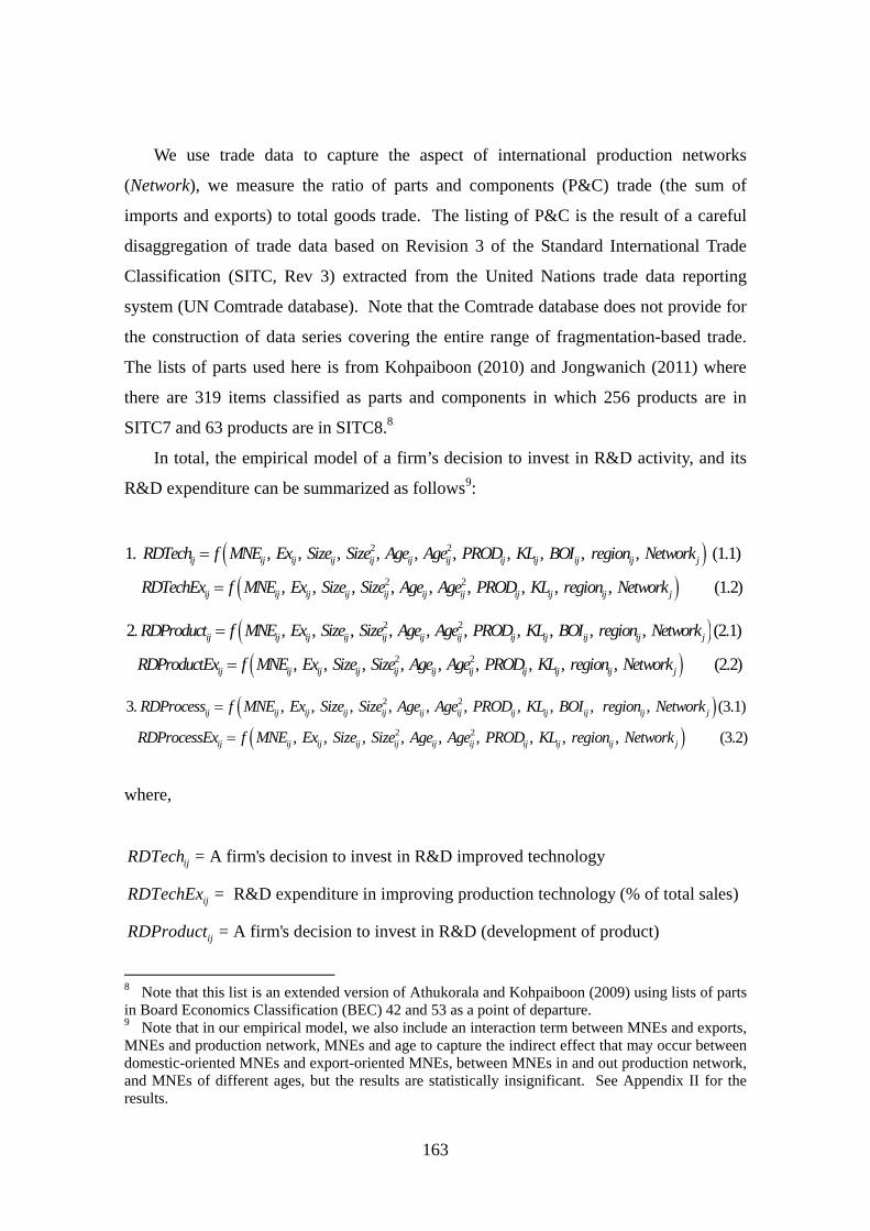
163  

We use trade data to capture the aspect of international production networks

(Network), we measure the ratio of parts and components (P&C) trade (the sum of

imports and exports) to total goods trade. The listing of P&C is the result of a careful

disaggregation of trade data based on Revision 3 of the Standard International Trade

Classification (SITC, Rev 3) extracted from the United Nations trade data reporting

system (UN Comtrade database). Note that the Comtrade database does not provide for

the construction of data series covering the entire range of fragmentation-based trade.

The lists of parts used here is from Kohpaiboon (2010) and Jongwanich (2011) where

there are 319 items classified as parts and components in which 256 products are in

SITC7 and 63 products are in SITC8.8

In total, the empirical model of a firm’s decision to invest in R&D activity, and its

R&D expenditure can be summarized as follows9:

2 2

2 2

1. , , , , , , , , , , (1.1)

, , , , , , , , ,

ij ij ij ij ij ij ij ij ij ij ij j

ij ij ij ij ij ij ij ij ij ij j

RDTech f MNE Ex Size Size Age Age PROD KL BOI region Network

RDTechEx f MNE Ex Size Size Age Age PROD KL region Network

(1.2)

2 2

2 2

2. , , , , , , , , , , (2.1)

, , , , , , , , ,

ij ij ij ij ij ij ij ij ij ij ij j

ij ij ij ij ij ij ij ij ij ij j

RDProduct f MNE Ex Size Size Age Age PROD KL BOI region Network

RDProductEx f MNE Ex Size Size Age Age PROD KL region Network

(2.2)

2 2

2 2

3. , , , , , , , , , , (3.1)

, , , , , , , , ,

ij ij ij ij ij ij ij ij ij ij ij j

ij ij ij ij ij ij ij ij ij ij

RDProcess f MNE Ex Size Size Age Age PROD KL BOI region Network

RDProcessEx f MNE Ex Size Size Age Age PROD KL region Networ

(3.2)jk

where,

A firm's decision to invest in R&D improved technologyijRDTech =

R&D expenditure in improving production technology (% of total sales)ijRDTechEx =

A firm's decision to invest in R&D (development of product)ijRDProduct =

                                                            8 Note that this list is an extended version of Athukorala and Kohpaiboon (2009) using lists of parts in Board Economics Classification (BEC) 42 and 53 as a point of departure. 9 Note that in our empirical model, we also include an interaction term between MNEs and exports, MNEs and production network, MNEs and age to capture the indirect effect that may occur between domestic-oriented MNEs and export-oriented MNEs, between MNEs in and out production network, and MNEs of different ages, but the results are statistically insignificant. See Appendix II for the results.

 

164  

R&D expenditure in product development (% of total sales)ijRDProductEx =

A firm's decision to invest in R&D (process innovation)ijRDProcess =

R&D expenditure in process innovation (% of total sales)ijRDProcessEx =

= Proportion of foreign share holding in a firm iijMNE

= Propensity to exportsijEx

= Size of firm i in industry jijSize

ij years ofoperation of firm i in industry j Age

ij Productivity of firm i in industry j PROD

= Capital-labor ratioijKL

= Investment (R&D) promotion from Board of Investment (BOI)ijBOI

Location of plant

(1 for Bankok, vicinity and central region and 0 otherwise)

ijregion

= International production network in industry jjNetwork

For the R&D spillovers, R&D and foreign ownership variables in equations (1.1, 2.1

and 3.1) are modified as follows:

2 2, , , , , , , , , , ,ij d j ij ij ij ij ij ij ij ij ij jRDTech f FOR Ex Size Size Age Age PROD KL BOI region Network

(4)

2 2, , , , , , , , , , ,ij d j ij ij ij ij ij ij ij ij ij jRDProduct f FOR Ex Size Size Age Age PROD KL BOI region Network (5)

2 2, , , , , , , , , , ,ij d j ij ij ij ij ij ij ij ij ij jRDProcess f FOR Ex Size Size Age Age PROD KL BOI region Network (6)

where

,ij dRDTech ; ,ij dRDProduct ; ,ij dRDProcess include only domestically-own firms and

jFOR = the presence of multinational firms in industry j

 

165  

5. Data and Econometric Procedure

Data for the study are compiled from unpublished returns to the Industrial Census

2006, the latest industrial census available, conducted by the National Statistics Office

(NSO). A well-known limitation of any cross-sectional data set, with each industry

representing a single data point, is that it is difficult to control for unobserved industry

specific differences. Long-term averages tend to ignore changes that may have occurred

over time in the same country. These limitations can be avoided by using a panel data

set compiled by pooling cross-industry and time-series data. Particularly, in the case of

technology spillover involving a time-consuming process, panel data are more

appropriate. Unfortunately, given the nature of data availability in this case, this

preferred data choice is not possible. So far there are two industrial census sets, i.e.

1996 and 2006, both are establishment-level data. Even though both of them provide an

establishment identification number, the number was not assigned systematically. Thus

for a given ID No., an establishment in 1996 is not necessarily the same as that in 2006.

The census covers 73,931 plants, classified according to the four-digit industries of

the International Standard of Industrial Classification (ISIC). The census was cleaned

up first by checking for duplicated samples. As occurred in the 1996 industrial census,

there are some duplicated records in the survey return, presumably because plants

belonging to the same firm filled in the questionnaire using the same records. The

procedure followed in dealing with this problem was to treat records reporting the same

value for the eight key variables of interest in this study as one record. The eight

variables are registered capital, number of male workers, number of female workers,

sale value, values of (initial and ending periods) capital stocks, value of intermediates

and initial stock of raw materials. There are 8,645 such cases so that the final sample

drops to 65,286 plants. In addition, we deleted establishments which had not responded

to one or more the key questions such as sales value or, output and which had provided

seemingly unrealistic information such as negative output value or an initial capital

stock of less than 5,000 baht (less than $200).10

                                                            10 If we alter initial capital to 10,000 baht the number to be dropped increased to 1,289 samples (another 500 samples dropped).

 

166  

The 2006 census contains a large number of micro-enterprises defined as plants

with fewer than 10 workers. There are 37,042 establishments in the sample which

employ less than 10 workers, 52% of which are micro enterprises which do not hire paid

workers (zero paid workers). The problem of self-employed samples is less severe

when considering the samples with more than 10 workers. Hence, our analysis focuses

on establishments with more than 10 workers net of self-employed firms. Seven

industries are excluded. These either serve niches in the domestic market (e.g.

processing of nuclear fuel, manufacture of weapons and ammunition), in the service

sector (e.g. building and repairing of ships, manufacture of aircraft and spacecraft, and

recycling) or are explicitly preserved for local enterprises (e.g. manufacture of ovens,

furnaces and furnace burners, manufacture of coke oven products). In total the

remaining establishments accounted for 75% of Thailand’s manufacturing gross output

and 62% of manufacturing value added in 2006.

Trade data are compiled from UN Comtrade and the standard concordance between

ISIC and HS code is used. Concentration ratio (CR4), which is used as an instrument

variable for exports, is obtained from Kophaiboon and Ramstetter (2008) in which the

concentration is measured at the more aggregate level (e.g. many measured at the 4-

digit whereas some at the 3-digit ISIC classification). This guards against possible

problems arising from the fact that two reasonably substitutable goods are treated as two

different industries according to the conventional industrial classification at a high level

of disaggregation.11 Tables 4 and 5 provide a statistical summary as well as a

correlation matrix of all relevant variables in this analysis.

                                                            11 Effective rate of protection is also used as alternative instrument variable for exports. It is calculated based on official data provided by Customs Department, Ministry of Finance (see Jongwanich and Kohpaiboon,, 2007). However, the model using concentration ratio as an instrument performs better in terms of diagnostic tests.

 

167  

Table 4. Statistics Summary of Variables

Observations Mean Std. Dev. Min Max

MNE, Share of foreign firms (%) 27,358 0.08 0.27 0 1

MNE, foreign participation (dummy 0 and 1) 27,358 4.65 18.33 0 100

Ex, Export share in total sales (%) 27,358 8.29 23.86 0 100

Ex, export participation (dummy 0 and 1) 27,358 0.16 0.37 0 1

Age, Firm age (Years) 27,358 12.17 9.92 1 99

PROD, Firm’s productivity (million baht/worker) 26,125 4.2 2.26 0 191

Sales, Firm size (million baht) 27,358 195 2240 0 279000

KL, capital-labor ratio (million baht/person) 27,358 0.57 6.43 0 670

Network, international production network (P&C trade to total trade)

27,358 0.02 0.09 0 1

RDTech, Decision to invest in R&D production technology (dummy 0 and 1)

27,358 0.06 0.23 0 1

RDTechEx, R&D production technology intensity (% of total sales)

27,358 0.2 1.87 0 100

RDProduct, Decision to invest in R&D production innovation (dummy 0 and 1)

27,358 0.06 0.24 0 1

RDProductEx, R&D production innovation (% of total sales)

27,358 0.29 2.82 0 100

RDProcess, Decision to invest in R&D process innovation (dummy 0 and 1)

27,358 0.04 0.2 0 1

RDProcessEx, R&D process innovation (% of total sales)

27,358 0.14 1.56 0 100

Concentration ratio 27,358 0.46 0.09 0.32 0.69

ERP, Effective rate of protection 27,358 0.12 0.35 -1.58 0.62

Source: Authors’ Compilation.

 

168  

Table 5. Correlation Coefficient Matrix A. A Firm’s Decision to Invest in R&D

RDTechij RDProductij RDProcessij Ageij Sizeij Klij Exij MNEij BOIij Networkij Regionij Productivityij

RDTechij 1

RDProductij 0.68 1

RDProcessij 0.64 0.64 1

Ageij 0.14 0.16 0.13 1

Sizeij 0.24 0.25 0.21 0.37 1

Klij 0.18 0.18 0.15 0.36 0.53 1

Exij 0.17 0.16 0.11 0.13 0.32 0.18 1

MNEij 0.12 0.12 0.1 0.08 0.28 0.21 0.36 1

BOIij 0.24 0.23 0.18 0.18 0.4 0.26 0.73 0.4 1

Networkij 0.05 0.03 0.03 0.05 0.15 0.1 0.11 0.17 0.12 1

Regionij 0.14 0.18 0.14 0.28 0.42 0.47 0.17 0.19 0.23 0.14 1

Productivityij 0.17 0.21 0.2 0.39 0.84 0.69 0.23 0.24 0.31 0.13 0.53 1

B. R&D Intensity (Improved Production Technology)

RDTechexij Ageij Sizeij Klij Exij MNEij BOIij Networkj Regionij Productivityij

RDTechexij 1

Ageij 0.0089 1

Sizeij -0.1123 0.2577 1

Klij -0.0503 0.0229 0.2748 1

Exij -0.061 -0.0164 0.2175 -0.1136 1

MNEij -0.041 0.014 0.2733 0.0871 0.2452 1

BOIij -0.0532 0.0893 0.3332 0.0185 0.6448 0.2527 1

Networkj 0.0913 -0.0306 0.0631 -0.0526 0.0743 0.19 0.0321 1

Regionij -0.0953 0.1159 0.3069 0.0794 0.0311 0.1088 0.1275 0.0528 1

Productivityij -0.0299 0.3923 0.8788 0.6895 0.2264 0.2381 0.3091 0.1293 0.5376 1

Note: Observations for the correlation are 1,046.

 

169  

C. R&D Intensity (Product Innovation) RDProductExij Ageij Sizeij Klij Exij MNEij BOIij Networkj Regionij Productivityij

RDProductExij 1 Ageij -0.0376 1 Sizeij -0.0899 0.2823 1 Klij -0.0856 0.0346 0.2956 1 Exij -0.0207 0.0296 0.2292 -0.0529 1 MNEij -0.0327 0.0318 0.2514 0.1424 0.2635 1 BOIij -0.0188 0.1085 0.3267 0.0306 0.6181 0.2521 1 Networkj 0.0706 -0.025 0.0431 -0.0376 0.0619 0.0963 -0.0009 1 Regionij -0.1457 0.0993 0.2811 0.1044 0.0192 0.0782 0.0724 0.0337 1

Productivityij -0.0293 0.1884 0.6414 0.4186 -0.0256 0.2349 0.1333 0.2885 0.2885 1 Note: Observations for the correlation are 1,218.

D. R&D Intensity (Process Innovation) RDProcessExij Ageij Sizeij Klij Exij MNEij BOIij Networkj Regionij Productivityij

RDProcessExij 1

Ageij 0.005 1

Sizeij -0.0939 0.2587 1

Klij -0.0786 0.0187 0.2795 1

Exij -0.0452 0.0859 0.2345 -0.0915 1

MNEij -0.0298 0.0446 0.2757 0.0919 0.2749 1

BOIij -0.0503 0.1212 0.3499 0.0387 0.6147 0.2139 1

Networkj 0.0774 -0.0264 0.0852 -0.0356 0.0771 0.1554 0.0053 1

Regionij -0.1061 0.0696 0.2413 0.0647 -0.032 0.0959 0.0751 0.0549 1

Productivityij -0.0791 0.1226 0.6314 0.4423 -0.0506 0.2268 0.0918 0.0408 0.0408 1

Note: Observations for the correlation are 762.

 

170  

5.1. Econometric Procedure

To examine a firm’s R&D decision and R&D spillovers (equations 1.1; 2.1; 3.1; 4;

5; 6), the probit model is applied. There are two key problems relating to OLS

estimation under a binary dependent variable, i.e. 1 for firms that export and 0

otherwise. First, the predicted value of a dependent variable under OLS could be higher

than 1 or could become negative. Secondly, linear relationship between dependent and

independent variables are generally assumed. However, the relationship between the

probability of investing in R&D and explanatory variables could be non-linear. To limit

the predicted value of a dependent variable so that it lies between 0 and 1, the Probit

model is applied. The Probit model is as follows:

*ij ij i ijg x e (7)

where *ijg is the binary dummy variable (i.e. taking the value of 0 and 1) to reflect a

firm’s R&D’s decision, ijx represents the explanatory variables listed in Section IV and

ije is the error term.

To deal with the endogeneity issue, especially for exports, the instrumental variable

method is applied with the probit model (IV probit) (Criscuolo et al., 2005). Instrument

variables are those that statistically affect/determine exports but are not statistically

significant in determining R&D. The effective rate of protection (ERP) and the

concentration ratio (CR4) are used as instrumental variables.12 Based on diagnostic

tests, we found that the concentration ratio performs better as an instrument variable

than the effective rate of protection. Thus, we use concentration as a key instrument

variable in this study.

To estimate a firm’s R&D expenditure (equation 1.2; 2.2; 3.2), the sample selection

model is applied since the dependent variable (i.e. R&D expenditure) is observed only

when a firm makes the decision to invest in R&D (i.e. could be observed only for a

restricted, nonrandom sample). There are two key equations in the model. The first

equation (equation (8)) explains whether an observation is in the sample or not while the

                                                            12 See Jongwanich and Kohpaiboon (2008) for analytical and empirical studies of how the effective rate of protection and market structure (the concentration ratio) affect a firm’s exports.

 

171  

second equation (equation (9)) determines the value of Y. Note that Y is the outcome

variable, which is only observed when a variable Z is positive.

* *i i iZ w e

*

*

0 0

1 0

i i

i i

Z if Z

Z if Z

(8)

* 'i i iY x

* Z 1

not observed Z 0i i i

i i

Y Y if

Y if

(9)

When equations (8) and (9) are solved together, the expected value of the variable Y is

the conditional expectation of *iY conditioned on it being observed (Zi = 1).

'

* '

'

' '

/ , / 1, ,

i

i i i i i i i i

i

i i

wE Y x w E Y d x w x

w

= x w

(10)

where 'iw ' '/i iw w is the inverse Mills ratio. It is important to note that

/ ,i i iE Y x w = 'ix if the two error terms are uncorrelated, i.e. 0 . In other words,

if two error terms are correlated, the simple OLS approach is inefficient and biased to

explain Y, so that we need to take into account the inverse Mills ratio by applying either

the Maximum Likelihood method (simultaneously estimating equations (8) and (9)) or

Heckman two-step estimation.

In this study, we apply two-step estimation since the model needs to take into

account the possible endogeneity problem that could arise, especially for the export

variable. The estimation procedure is as follows. First, we construct the inverse Mills

ratio from the probit model (IVprobit model) for each type of R&D (equation 7) and

then estimate equations 1.2; 2.2; 3.2, using a cross-sectional model and include the

 

172  

inverse Mills ratio as additional regressor. Note that instrumental variable method is

also applied at this stage.

6. Results

Tables 6, 7 and 8 report the results of a firm’s R&D investment in improved

production technology, product development, and process innovation, respectively. In

each table, there are two columns. Columns A present the determinants of a firm’s

R&D decision, which take a value of ‘1’ for a firm engaging in R&D activity and ‘0’

otherwise, whereas columns B show determinants of a firm’s R&D intensity. Table 9

presents the determinants of R&D spillover for improved production technology

(column A), product development (column B), and process innovation (column C).

The model shows the negative and statistically significant relationship between

multinational firms (MNEs) and a firm’s decision to invest in R&D leading to improved

production technology and leading to product development, but not in R&D leading to

process innovation. Given the fact that nearly half of world R&D expenditure was

undertaken by MNEs (UNCTAD, 2005), the negative and statistically significant

coefficient implies that most MNE affiliates are unlikely to invest in R&D in the host

country (Thailand), but instead they are likely to import technology (technology

transmission) from their parent company. In terms of improved production technology,

this is plausible since R&D investment in such activity involves high fixed costs, at a

time when transportation costs have become cheaper, so that it tends to be more

efficient to invest in R&D activity at their headquarters and import technology to the

host country. In addition, the decentralization of R&D activity relating to production

technology has a high risk of leakage of propriety assets, which is important to MNEs

wishing to retain their ownership advantage in international operation.

 

173  

Table 6. Estimation Results of R&D Leading to Improved Production Technology

(Both Domestic and Foreign Firms)

Column A Column B

A firm’s decision to invest in R&D R&D intensity (% of sales)

Coefficient T-statistics Coefficient T-statistics

Intercept -12.37 -9.81* -5.6 -0.57

MNEij -11.12 -1.58** 75.57 0.48

Exij 0.95 1.38 -3.29 -0.52

Ageij 0.07 2.69* -0.13 -0.35

Ageij^2 - - - -

PRODij -0.08 -3.51* -0.16 -0.44

Sizeij 0.99 7.61* 1.06 0.61

Sizeij^2 -0.02 -5.99* -0.03 -0.66

KLij 0.07 4.67* -0.21 -0.55

BOIij -0.12 -0.37 - -

regionij 0.02 0.41 -0.45 -0.72

Networkj 0.46 2.48* 1.23 1.43

Inversed mill ratio - 2.24 0.52

No. of obs 17,427 1018

Log likelihood 5274.8 Root MSE = 1.40

Wald chi2 1257.19 (Prob>chi2 = 0.00)

Wald-test for exogeneity 1.37 (Prob>chi2 = 0.24)

Note: (1) Column A is estimated by IVProbit model using concentration ratio as the instrument for exports and Column B is estimated by 2SLS and sample-selection model. Logarithm is used for Age; Size; KL while a ratio is applied for MNE (the share of foreign firms); EX (the share of exports to total sales); and Network (the share of trade in parts and components to total trade).

(2) *, **, and *** indicate the significance level at 5, 10 and 15%, respectively, and

(3) Industrial dummy variables are included (according to ISIC) in the estimation.

Source: Authors’ estimations.

In terms of product development, the innovatory process involves rich

communication and cooperation within a firm, between product design, the production

team, marketing etc, and a face to face communication. In other words, close

interdepartmental relationships and teamwork are required for the development of

innovation. Thus, it would be more efficient for the MNEs to develop/innovate new and

core products in their headquarters, instead of decentralizing such activity to their MNE

affiliates. This is especially true in the context of small and long-open developing

economies like Thailand. However, MNEs still listen and gather information from their

 

174  

affiliates to ensure that the innovated products can match well with consumer preference

in different locations.

The statistical insignificance found in R&D leading to process innovation implies

that some MNEs began to invest in R&D leading to process innovation in the host

country, including introducing “lean processing” and “just in time” methods, but their

likelihood of conducting such R&Ds is not statistically different from that of their local

firms.

Table 7. Estimation Results of R&D Product Development (Both Domestic and

Foreign Firms)

Column A Column B

A firm’s decision to invest in R&D R&D intensity (% of sales)

Coefficient T-statistics Coefficient T-statistics

Intercept -11.64 -9.38* -0.94 -0.4

MNEij -16.28 -2.52 6.32 0.21

Exij 1.9 3.15* -0.44 -0.31

Ageij 0.12 4.89* -0.04 -0.4

Ageij^2 - - - -

PRODij -0.09 -4.10* 0.06 0.86

Sizeij 1 8.04* 0.25 0.81

Sizeij^2 -0.02 -6.53* -0.008 -1.04

KLij 0.04 3.18* -0.06 -1.31

BOIij -0.6 -2.15* - -

regionij 0.25 5.19* -0.44 -2.28*

Networkj 0.5 2.87* 0.7 2.22*

Inverse mill ratio - 0.1 0.22

No. of obs 17,951 1,191

Log likelihood 5045.81 Root MSE = 0.980

Wald chi2 1797.91 (prob>chi2 = 0.00)

Wald-test for exogeneity 0.33 (prob>chi2 = 0.56)

Note: (1) Column A is estimated by IVProbit model using concentration ratio as the instrument for exports and Column B is estimated by 2SLS and sample-selection model. Logarithm is used for Age; Size; KL while a ratio is applied for MNE (the share of foreign firms); EX (the share of exports to total sales); and Network (the share of trade in parts and components to total trade).

(2) *, **, and *** indicate the significance level at 5, 10 and 15%, respectively and

(3) Industrial dummy variables are included (according to ISIC) in the estimation.

Source: Authors’ estimations.

 

175  

Table 8: Estimation Results of R&D Process Innovation (Both Domestic and

Foreign Firms)

Column A Column B

A firm’s decision to invest in R&D R&D intensity (% of sales)

Coefficient T-statistics Coefficient T-statistics

Intercept -11.9 -8.74* 2.87 0.49

MNEij -8.68 -1.1 -10.56 -0.25

Exij 0.2 0.25 0.48 0.23

Ageij 0.35 2.49* 0.04 0.12

Ageij^2 -0.04 -1.56** 0.002 0.04

PRODij -0.12 -4.49* 0.02 0.15

Sizeij 0.91 6.37* -0.2 -0.27

Sizeij^2 -0.02 -4.69* 0.004 0.21

KLij 0.05 2.97* -0.009 -0.13

BOIij 0.06 0.17 - -

regionij 0.13 2.22* -0.13 -0.48

Networkj 0.07 0.34 0.65 1.82**

Inverse mill ratio - 0.02 0.05

No. of obs 17,998 748

Log likelihood 5945.38 Root MSE = 0.92

Wald chi2 1028 (prob>chi2 = 0.00)

Wald-test for exogeneity 0.00 (prob>chi2 = 0.95)

Note: (1) Column A is estimated by IVProbit model using concentration ratio as the instrument for exports and Column B is estimated by 2SLS and sample-selection model. Logarithm is used for Age; Size; KL while a ratio is applied for MNE (the share of foreign firms); EX (the share of exports to total sales); and Network (the share of trade in parts and components to total trade).

(2) *, **, and *** indicate the significance level at 5, 10 and 15%, respectively, and

(3) Industrial dummy variables are included (according to ISIC) in the estimation.

Source: Authors’ estimations.

In contrast to MNEs, a positive sign is found for the exporting variable. However,

the model shows the positive, but statistically insignificant, relationship between

exporting and a firm’s decision to invest in R&D leading to improved production

technology and leading to process innovation (Tables 6 and 8). The statistical

insignificance implies that the probability of firms to investing in R&D for improving

production technology and for process innovation is not affected by market destination,

i.e. either domestic or export markets. By contrast, we find a positive and statistically

significant relationship between exports and a firm’s decision to invest in product

development R&D (Table 7), reflecting the idea that exporters tend to learn more about

 

176  

competing products and customer preferences in international markets, but the

information gained relating to improving production technology and process innovation

is limited. The information on competing products and customer preferences could

come from customer feedback, export intermediaries and other foreign agents. Thus,

information passed from foreign customers helps firms innovate/tailor their products to

meet the specific needs of international markets. It is noteworthy that although the

relationship of exports and the other two R&D activities is statistically insignificant, the

positive sign of this variable could, to some extent, reflect the idea intense global

competition may begin to stimulate firms to invest in R&D leading to improved

production technology and processes.

The model also shows that firm age and firm size have a positive and significant

impact in determining a firm’s decision to invest in R&D for improved production

technology and R&D product development. The positive sign of firm age in these two

R&D equations supports the argument that older firms tend to be more likely to change

production processes and adopt new technologies than younger firms. Interestingly, for

R&D process innovation, we find that (Age^2) is negative, while there is statistical

significance, along with a significantly positive sign for Age. This implies that the

incentive for firms to invest in process innovation grows at a diminishing rate and

becomes negative when the firms reach a certain years of age. In this study, we find that

when firm age is over 70 years, the probability of firms investing in R&D for process

innovation becomes negative (Table 8). Note that the negative signs of Age^2 are also

found in R&D for improved production technology and R&D for product development,

but that these signs are statistically insignificance (See Appendix I for this result).

A non-linear relationship between firm size (Sizeij) and a decision of a firm to invest

in R&D activity is also found in this study. The positive sign for firm size reflects the

fact that R&D activity involves high fixed costs. However the capital market is

imperfect so that larger firms, which are likely to have stable funding access are able to

afford R&D investment as opposed to smaller firms. However, the negative sign for

Size^2 shows that this factor would become less important in affecting a firm’s decision

to invest in all three types of R&Ds when it reaches a certain level. In other words, after

the firm reaches its break-even point, other factors would become more important for

 

177  

the firm’s decision making. In this study, such a level of firm size, measured by annual

sales, would be around 126 billion baht.

In addition to firm age and firm size, our study finds a negative and statistically

significant relationship between a firm’s productivity (PRODij) and its decision to invest

in all three types of R&D. This result is in contrast to the expected positive sign, which

is mentioned in Section IV. The negative relationship found in this study implies that

the probability of a firm with lower productivity investing in all types of R&D would be

higher than for a firm with high productivity. This tends to reflect a possible catching

up process among firms, not only to improve their own productivity, but also to survive

in an intensely competitive environment. The coefficient corresponding to this variable

is the highest for R&D leading to process innovation, followed by R&D leading to

product development and improved production technology. This may reflect the fact

that where a firm’s productivity improvement is concerned, the process innovation

mode seems to be prioritized before improving production technology, with its

relatively higher fixed costs.

The model also shows that firms in a more capital-intensive industry have a higher

probability of involvement in all three types of R&D activities, confirming that the

nature of its industry could influence a firm’s decision to invest in R&D. While the

possible causality between R&D and the industry’s capital intensity can occur in theory,

it is unlikely in reality because it takes time for R&D investment to result in capital

deepening. This argument is in line with what Aw et al. (2008) which used lagged

instead of current R&D investments in the productivity equation. This study also finds

that infrastructure tends to be one of the crucial factors that positively influence a firm’s

decision to invest in all three types of R&Ds. This is reflected by the positive

relationship of “region” to a firm’s decision to invest in R&Ds.

A statistically insignificant relationship between government policy (BOI) and a

firm’s R&D decision is found in R&D leading to improved production technology and

leading to process innovation.13 This result could, to some extent, reflect the thought

that government policy so far has not been effective enough to influence a firm’s                                                             13 Note that the insignificance of this variable may arise from the fact that the available measurement of government policy used here could not capture well the overall policies implemented by the government. Disaggregated details of government policy in each industry, which so far are not available, may help to improve accuracy of our model.

 

178  

decision to set up an R&D activity. By contrast, other fundamental variables, such as

firm age, firm size, firm productivity, and other industrial characteristics, play more

crucial roles in influencing the firm’s decision making. However, when we consider

only domestically-owned firm in R&D spillover (see more detail below), government

policy (BOI) positively increases the probability of a firm investing in R&D, especially

in terms of improved production technology. Thus, the insignificant effect of BOI

found here tends to be dominated by foreign firms, most of whose decisions are

influenced by their parent companies (i.e. by firm specific factors), and for whom

government policy is less relevant. Government policy, by contrast, tends to affect

more the decisions of domestically-owned firms in setting up R&D activities, since

most are disadvantaged in terms of proprietary assets and need more support from

government.

Another interesting result is the ‘network’ variable. The positive relationship of

“network” and a firm’s decision to invest in R&D supports the importance of

international production networks in promoting a firm’s R&D decision. The dynamism

of industries involved in production networks is likely to require more R&D investment

to keep the industry upbeat and competitive in the international market. “Network” is

also statistically significant and positive not only for a firm’s basic R&D decisions, but

also for intensity for all three types of R&D. This implies that the higher the importance

of the international production network to a firm, the greater the R&D expenditure

expected. The robust econometric evidence here encourages developing countries to

participate in MNE production networks.

Except for “network”, other variables are statistically insignificant in the R&D

intensity equations (equations 1.2; 2.2 and 3.2). The inability to capture well their

relationship could be due to the smaller sample size of firms who are involved in R&D

activity. In addition, the variation of R&D expenditures is limited among these firms.

For example, in R&D for improved production technology there are only 1,558 firms

who decided to set up an R&D activity and the R&D expenditures are mostly set by less

than, or equal to, 10% of total expenditure. The low variation of R&D expenditure

makes it rather difficult to reveal the relationship statistically.

 

179  

6.1. R&D spillovers

Interestingly, although there is evidence that most multinational firms tend to import

technology, instead of establishing R&D activity in the host country (i.e. statistical

insignificance between a firm’s decision to invest in R&D and MNEs), multinational

firms do tend to stimulate domestically-owned firms to invest more in R&D activity

(i.e. spillovers). Such evidence is supported by the positive sign and statistical

significance of the share of foreign ownership at the industry level (FORj) and a

domestically-owned firm’s R&D decision (Table 9). Among the three types of R&D

activity, the spillover tends to be strong in product development, followed by process

innovation, while there is statistical insignificance in the case of product technology.

The strong spillovers in product development and process innovation support the idea of

the important process of demonstration and imitation in generating R&D spillovers.

Intense competition from the entry of MNEs might play some role in generating

spillover and encouraging domestic firms to invest in R&D and reduce costs. However,

the statistical insignificance of FOR in the R&D improved production technology

equation could be because of the relatively high fixed costs of such investment. This

may limit the possible positive effect that could arise from demonstration and imitation

effects.

 

180  

Table 9. Estimation Results of R&D Spillovers (The Domestically-owned Firms’ Decision to Invest in R&D)

Column A Column B Column C

R&D improved technology R&D product development R&D process innovation

Coefficient T-statistics Coefficient T-statistics Coefficient T-statistics

Intercept -14.01 -10.85* -12.23 -8.90* -12.78 -11.03*

FORj 0.004 1.38 0.004 1.70** 0.003 1.76**

Exij -1.23 -1.18 1.34 1.45*** -2.02 -1.2

Ageij 0.05 1.66** 0.1 3.64* 0.17 1.56**

Ageij^2 - - - - -0.02 -0.81

PRODij -0.14 -5.61* -0.14 -5.48* -0.14 -6.59*

Sizeij 1.06 7.19* 1.02 7.29* 0.92 6.51*

Sizeij^2 -0.02 -5.39* -0.02 -5.64* -0.02 -4.60*

KLij 0.1 5.90* 0.06 4.24* 0.07 4.71*

BOIij 0.88 1.97* -0.29 -0.7 1.08 1.49***

regionij -0.02 -0.41 0.22 4.24* 0.06 1.19

Networkj 0.4 1.64** 0.64 2.92* - -

No. of obs 16,245 16,245 16,289

Log likelihood 7344.29 7095.7 10290.9

Wald chi2 1157.4 (prob>chi2 = 0.00) 1370.4 (prob>chi2 = 0.00) 1 (prob>chi2 = 0.00)

Wald-test for exogeneity 1.63 (prob>chi2 = 0.20) 1.77 (prob>chi2 = 0.18) 1.04 (prob>chi2 = 0.31)

Note: (1) Column A is estimated by IVProbit model using concentration ratio as the instrument for exports and Column B is estimated by 2SLS and sample-selection model. Logarithm is used for Age; Size; KL while the ratio is applied for MNE (the share of foreign firms); EX (the share of exports to total sales); and Network (the share of trade in parts and components to total trade). (2) *, **, and *** indicate the significance level at 5, 10 and 15%, respectively, and (3) Industrial dummy variables are included (according to ISIC) in the estimation.

Source: Authors’ estimations.

 

181  

The model shows the mild significance of exporting on the firm’s decision to invest

in R&D leading to product development while there is no positive and significant effect

of exports on firm’s its decision to invest in R&D leading to production technology and

process innovations. This is consistent with the above finding when we include both

domestic and foreign firms, i.e. entering export markets tends to help firms get/learn

more information about products and consumer preferences than about production

technology and process innovation. However, the smaller coefficient of this variable,

compared to the situation where we consider both foreign and domestic firms, reflects

the fact that domestic firms still have limited knowledge of world market, especially in

terms of networking, compared to foreign firms. In addition, despite statistical

insignificance, the negative relationship between exporting and a firm’s decision to

invest in R&D for production technology might reflect the fact that domestically-owned

firms which export could access/update new production technology easier than other

domestic firms so that they are likely to import production technology, instead of

involving themselves in ‘technology generation’.

Regardless of foreign ownership, however, firm age, firm size, capital intensity and

location are all significant in affecting the decisions of domestically-owned firms in

investing in all types of R&D activity. Positive relationships of these variables and the

firm’s R&D decision are found. In particular, the non-linear relationship between firm

size and the firm’s R&D decision is revealed in all three types of R&D activity. The

catching up effect is still found in the case of domestically-owned firms, as suggested by

the negative sign and statistical significance of coefficients corresponding to a firm’s

productivity variable. A production network (network) tends to positively and

significantly affect the probability of a domestic firm investing in R&D for product

development and production technology, but there is no such evidence for R&D process

innovation.

 

182  

7. Conclusion and Policy Inferences

This paper examines the role of multinational enterprises (MNEs) and exporting on

R&D activity, using the most recent (2006) industrial census of Thai manufacturing,

with emphasis on providing useful policy suggestions for promoting R&D activities in

developing countries. The paper is distinguished from the existing literature in two

ways. First, R&D investment is categorized into three broad types, i.e. R&D leading to

improved production technology, product development, and process innovation. To the

best of our knowledge, this is one of the few studies undertaking research into possible

heterogeneity in firms’ decision toward on each type of R&D. Secondly, three key

globalization forces, namely MNEs, exporting, and global production networks, are

examined in a single framework over and above industry and firm-specific factors.

Our key findings suggest that the determinants of each R&D are far from identical.

For example, MNE affiliates would prefer to undertake process innovation-related R&D

locally but not R&D for production technology and product development. Another

example is the propensity for, and intensity of product development R&D which can be

positively affected by exporting. Hence, our conclusion that separating the types of

R&D when examining its determinants is a necessary step in gaining a better

understanding of firms’ R&D activities.

Globalization through exporting and FDI can play a role in encouraging firms to

commit to R&D investment. Note that the role played by exporting seems to be

different from that played by FDI. We found a lower R&D propensity for MNE

affiliates than for locally-owned firms, pointing to the fact that MNEs prefer importing

technology from their parent companies to developing new technology in host countries.

Nonetheless, this does not indicate that there is no effect from MNE presence on R&D

propensity and intensity. In fact, their presence could stimulate locally-owned firms to

undertake R&D activities. The latter might set up in-house R&D facilities in order to

reap potential and possible technological benefits from the MNE presence in a given

industry. In addition, firms participating in global production networks are more active

in all types of R&D activity than those not participating. Considered together with their

 

183  

relative importance in the global production networks, this result would be another

indirect contribution by MNEs and globalization.

Exporting, the other globalized force, tends to have a positive and significant

impact, but its impact is limited to R&D leading to product development, and it does not

impact the other two types of R&D. This implies that entering export markets tends to

help firms to learn more about competing products and customer preferences, but

information relating to improving the technology of production, and process innovation,

is still limited.

From the policymakers’ perspective, three policy suggestions can be drawn from

our study. The first concerns the role of government policy. Supply-side capability,

such as infrastructure services, is highlighted in this study. Improving infrastructure

could eventually attract more foreign direct investment into the host country, generating

spillover impacts on domestically-owned firms. In addition to infrastructure,

government should improve other aspects of the business environment, including trade

facilitation, to further promote FDI so that the indirect impacts of MNEs on R&D

activity in the host country could be increased. Our study raises concerns about relying

heavily on policy-induced incentives such as tax exemptions, to spur R&D activity. The

effectiveness of these policy measures is not always apparent. Secondly, our findings

provide evidence to support ongoing globalization. Firms exposed to global

competition through either exporting or participating in global production networks are

more likely to commit to R&D investment. The net effect of MNEs on R&D activities

cannot be measured solely by whether MNEs conduct R&D activities in the host

country. Even though MNE affiliates do not invest in R&D locally, their presence still

stimulates local firms to become more active in R&D. Finally, the role of global

production networks and the relative importance of infrastructure services in this study

point to the area where plurilateral organizations such as ASEAN can play a role in

spurring R&D activities. Cooperation in infrastructure services among member

countries would facilitate the entry of MNEs seeking to utilize the specialization of the

the region in their global production networks, and could help locally owned firms to

become more likely to participate in global production networks. This eventually

results in an increase in R&D intensity.

 

184  

References

Acs, Z.J. and Audretsch, D.B. (1987), ‘Innovation, Market Structure, and Firm Size’, The Review of Economics and Statistics, 69:4, 567-74

ADB (2010), Asian Development Outlook 2010 Update: The Future of Growth in Asia. Asian Development Bank (ADB), Manila.

Athukorala, P. and Kohpaiboon, A., (2010), “Globalization of R&D by US-based Multinational Enterprises’, Research Policy, 39(10), 1335-347.

Aw, B.Y., Roberts, M., and Xu, D (2009), ‘R&D Investment, Exporting and Productivity Dynamics’, NBER Working Paper No. 14670, the National Bureau of Economic Research, Washington DC.

Aw, B.Y., Roberts, M.J., and Xu, D.Y. (2008), “R&D Investments, Exporting, and the Evolution of Firm Productivity’, American Economic Review, 98, 451-456

Barrios, B., Brulhart, M., Elliot, R. and Sensier, M. (2003), ‘A Tale of Two Cycles: Co-fluctuations between UK Regions and the Euro Zone’, The Manchester School, 71, 265–292

Clerides, S. K., Lach, S., and Tybout, J.R. (1998), ‘Is learning by Exporting Important? Micro Dynamic Evidence from Colombia, Mexico, and Morocco’, Quarterly Journal of Economics, 113, 903-947

Criscuolo, C., Haskel, J. and Slaughter, M. (2005), ‘Global Engagement and the Innovation Activities of Firms’, NBER Working Paper, 11479, Cambridge, MA

Daft, R.L., Lengel, R.H., Trevino, L.K. (1987), ‘Message Equivocality, Media Selection and Manager Performance: Implications for Information Systems’, MIS Quarterly, 11:3, 355-366

Doner, R. F. (2009), The Politics of Uneven Development. Cambridge: Cambridge University Press

Dorfman, N.S. (1987), ‘Innovation and Market Structure: Lessons from the Computer and Semiconductor Industries’, Cambridge, MA: Ballinger

Grossman G. and Helpman E. (1991), ‘Innovation and Growth in the Global Economy’, MIT Press, Cambridge MA.

Hirsch, S. and Bijaoui, I. (1985), ‘R&D Intensity and Export Performance: A Micro View’, Weltwirtschaftliches Archiv, 121, 238-251

Jongwanich, J (2011), ‘Foreign Direct Investment in Emerging Asia: Implications of the International Production Network’, in Firm-level internationalisation, regionalism and globalization, Elaine Hutson, Rudolf R. Sinkovics and Jenny Berrill (Eds.), London: Palgrave Macmillan (forthcoming).

Jongwanich, J and A. Kohpaiboon (2008), ‘Export Performance, Foreign Ownership and Trade Policy Regime: Evidence from Thai Manufacturing’, ERD Working Paper No. 140, Economics and Research Department, Asian Development Bank.’

 

185  

Jongwanich, J. and A. Kohpaiboon (2008), ‘Private Investment in Thailand: Patterns and Determinants’, World Development, 36(10), 1709-24

Jongwanich, J. and Kohpaiboon, A. (2007), ‘Determinants of Protection in Thai Manufacturing’, Economic Papers, 26:3, 276-94.

Kohpaiboon, A. (2010), ‘Import-as-market Discipline Hypothesis: Evidence of Thai Manufacturing Sector’, ERIA Micro-Data Project, Economic Research Institute for ASEAN and East Asia (ERIA), Jakatra

Kohpaiboon, A. and Ramstetter, E.D. (2008), ‘Foreign Ownership and Producer Concentration in Thai Manufacturing’, Working Paper 2008-05, Kitakyushu: ICSEAD.

Lall, S. (1979), ‘The International Allocation of Research Activity by US Multinationals’, Oxford Bulletin of Economics and Statistics, 41:4, 313-31

Lee, M.H. and Hwang, I.J. (2003), ‘Determinants of Corporate R&D Investment: An Empirical Study Comparing Korea's IT Industry with its non-IT Industry’, ETRI Journal, 25:4, 258-265

Levin, R.C., Klevorick, A.K., Nelson, R.R., and Winter, S.G. (1987), ‘Appropriating the Returns from Industrial Research and Development’, Brookings Papers on Economic Activity, 3 , 783-820

Lipsey, R.E. (2001), ‘Foreign Direct Investment and the Operations of Multinational Firms: Concepts, History, and Data’, NBER Working Papers 8665, National Bureau of Economic Research

Melitz, M.J. and Ottaviano, G.I.P., (2008), ‘Market Size, Trade, and Productivity,’ Review of Economic Studies, 75:1, 295-316

Meyer, J. (2009), ‘Workforce Age and Technology Adoption in Small and Medium-sized Service Firms’, Small Business Economics: 12-32

Mishra, V. (2007), ‘The Determinants of R&D Expenditure of Firms: Evidence from a Cross-section of Indian Firms’, Economic Papers, Economic Society of Australia, 26: 3, 237-248

NESDB & World Bank (2006), ‘Measuring Output and Productivity in Thailand’s Service-producing Industries’, A report collaborated between National Economics and Social Development Board (NESDB) and World Bank (Thailand), Bangkok.

Newark, P.D.L. (1983), ‘Further Evidence of the Determinants of Industrial Research and Development Using Single and Simultaneous Equation Model’, empirical economics, 8: 203-14.

Pavitt, K. (1987), ‘The Objectives of Technology Policy’, Science and Public Policy, 14, 182–188

Salomon R. and Shaver J.M. (2005), ‘Learning by Exporting: New Insights from Examining Firm Innovation’, Journal of Economics and Management Strategy, 14:2, 431–460

Schumpeter, J.A. (1942), Capitalism, Socialism and Democracy. New York: Harper

 

186  

Serapio, M. and D. Dalton (1999), ‘Globalization and Industrial R&D: An Examination of Foreign Direct Investment in R&D in the United States’, Research Policy, 28, 303-16

United Nations Conference on Trade and Development (2005), World Investment Report: TNCs and Internationalization of R&D. Geneva.

Vaona, A. and Pianta, M. (2008) ‘Firm Size and Innovation in European Manufacturing’, Small Business Economics, 30:3, 283-299

Vernon, R. (1979), ‘The Product Cycle in the New International Environment’, The Oxford bulletin of economics and statistics, 41, 255-267

Wakelin, K. (1998), ‘Innovation and Export Behaviour at the Firm Level’, Research Policy, 26, 829-841

Yusuf, S. and K. Nabeshima (2010), Tigers Under Threat: The Search for a New Growth Strategy by Malaysia and its Southeast Asian Neighbors. Oxford: Oxford University Press.

 

187  

APPENDIX 1

Example of Full Estimation Results of R&D Leading to Improved Production

Technology (both Domestic and Foreign Firms)

Column A

A firm’s decision to invest in R&D Column B

A firm’s decision to invest in R&D Coefficient T-statistics Coefficient T-statistics

Intercept -12.36 -9.78* -11.68 -2.29* MNEij -11.01 -1.57** -13.98 -0.66 Exij 0.95 1.37 1.49 0.40 Ageij 0.01 0.12 0.007 0.06 Ageij

^2 0.13 0.55 0.01 0.57 PRODij -0.08 -3.48* -0.08 -1.39 Sizeij 1.00 7.62* 0.97 4.10* Sizeij

^2 -0.02 -6.01* -0.02 -4.15* KLij 0.07 4.67* 0.07 3.97* CR4j - - -0.38 -0.14 BOIij -0.12 -0.37 -0.36 -0.21 regionij 0.02 0.39 0.02 0.43 Networkj 0.46 2.49* 0.56 0.73 No. of obs 17,427 17,427 Log likelihood 5277.86 5284.09 Wald chi2 1257.7 (Prob>chi2 = 0.00) 1315.3 (Prob>chi2 = 0.00) Wald-test for exogeneity

1.36 (Prob>chi2 = 0.24) 0.13 (Prob>chi2 = 0.72)

Note: (1) Column A is estimated by an IVProbit model using concentration ratio as the instrument for exports and Column B is estimated by including concentration ratio as one of the independent variables, and using the effective rate of protection as the instrument variable for exports. Logarithm is used for Age, Size and KL, while a ratio is applied for MNE (the share of foreign firms), EX (the share of exports to total sales) and Network (the share of trade in parts and components to total trade).

(2) *, **, and *** indicate the significance level at 5, 10 and 15%, respectively; and

(3) Industrial dummy variables are included (according to ISIC) in included in the estimation.

Source Authors’ estimate.

 

188  

Example of Full Estimation Results of R&D Leading to Product Development

(both Domestic and Foreign Firms)

Column A

A firm’s decision to invest in R&D Column B

A firm’s decision to invest in R&D Coefficient T-statistics Coefficient T-statistics

Intercept -11.62 -9.35* -9.71 -1.71** MNEij -16.17 -2.50* -22.09 -1.37 Exij 1.90 3.15* 3.01 1.04 Ageij 0.07 0.68 0.05 0.48 Ageij

^2 0.01 0.53 0.01 0.66 PRODij -0.09 -4.07* -0.07 -1.26 Sizeij 1.00 8.04* 0.91 2.90* Sizeij

^2 -0.02 -6.53* -0.02 -3.05* KLij 0.04 3.18* 0.04 2.45* CR4j - - -0.86 -0.36 BOIij -0.60 -2.14* -1.10 -0.83 regionij 0.25 5.17* 0.25 4.19* Networkj 0.50 2.87* 0.72 1.18 No. of obs 17,427 17,427 Log likelihood 5020.19 5026.70 Wald chi2 1640.4 (Prob>chi2 = 0.00) 2027.0 (Prob>chi2 = 0.00) Wald-test for exogeneity

0.01 (Prob>chi2 = 0.94) 0.75 (Prob>chi2 = 0.39)

Note: (1) Column A is estimated by an IVProbit model using concentration ratio as the instrument for exports and Column B is estimated by including concentration ratio as one of the independent variables, and using effective rate of protection as the instrument variable for exports. Logarithm is used for Age, Size and KL while a ratio is applied for MNE (the share of foreign firms); EX (the share of exports to total sales); and Network (the share of trade in parts and components to total trade).

(2) *, **, and *** indicate the significance level at 5, 10 and 15%, respectively; and

(3) Industrial dummy variables are included (according to ISIC) in included in the estimation.

Source: Authors’ estimations.

 

189  

Example of Full Estimation Results of R&D Leading to Process Innovation (both

Domestic and Foreign Firms)

Column A

A firm’s decision to invest in R&D Column B

A firm’s decision to invest in R&D Coefficient T-statistics Coefficient T-statistics

Intercept -11.90 -8.74* -3.52 -0.83 MNEij -8.67 -1.10 -33.24 -4.22* Exij 0.20 0.25 4.91 3.52* Ageij 0.35 2.49* 0.18 1.31 Ageij

^2 -0.04 -1.56** -0.02 -0.61 PRODij -0.12 -4.49* -0.03 -0.59 Sizeij 0.91 6.37* 0.50 1.89** Sizeij

^2 -0.02 -4.69* -0.01 -1.97* KLij 0.05 2.97* 0.03 1.88** CR4j - - -3.35 -0.09 BOIij 0.06 0.17 -2.07 -3.18* regionij 0.13 2.22* 0.12 2.54* Networkj 0.07 0.34 1.05 3.14* No. of obs 17,473 17,473 Log likelihood 5851.4 5859.1 Wald chi2 909.1 (Prob>chi2 = 0.00) 3062.0 (Prob>chi2 = 0.00) Wald-test for exogeneity

0.14 (Prob>chi2 = 0.71) 4.15 (Prob>chi2 = 0.05)

Note: (1) Column A is estimated by an IVProbit model using concentration ratio as the instrument for exports and Column B is estimated by including concentration ratio as one of the independent variables and using effective rate of protection as the instrument variable for exports. Logarithm is used for Age, Size and KL while a ratio is applied for MNE (the share of foreign firms); EX (the share of exports to total sales); and Network (the share of trade in parts and components to total trade).

(2) *, **, and *** indicate the significance level at 5, 10 and 15%, respectively, and

(3) Industrial dummy variables are included (according to ISIC) in included in the estimation.

Source: Authors’ estimations.

 

190  

APPENDIX II

Example of Full Estimation Results of R&D Leading to Improved Production

Technology (Interaction Terms) (both Domestic and Foreign Firms)

A firm’s decision to invest in R&D

Column A Column B Column B

Coefficient T-statistics Coefficient T-statistics Coefficient T-statistics Intercept -12.90 -11.21* -12.89 -11.19* -12.83 -11.10* MNEij -0.10 -0.01 -5.68 -0.94 -25.38 -1.31 Exij 0.35 1.80** 0.14 1.72** 0.14 1.74** Ageij 0.07 2.65* 0.07 2.66* -0.02 -0.20 Ageij

^2 - - - - - - PRODij -0.09 -4.06* -0.09 -4.06* -0.09 -4.09* Sizeij 1.01 7.79* 1.01 7.80* 1.02 7.88* Sizeij

^2 -0.02 -6.02* -0.02 -6.03* -0.02 -6.12* KLij 0.07 4.55* 0.07 4.58* 0.07 4.62* BOIij 0.24 4.16* 0.25 4.35* 0.25 4.35* regionij 0.01 0.27 0.02 0.32 0.02 0.34 Networkj 0.38 2.19* 0.45 0.95 0.38 2.18* MNEij*Exij -16.41 1.20 - - - - MNEij*Networkj - - -4.84 -0.15 - - MNEij*Ageij - - - - 7.57 1.05 No. of obs 17,427 17,951 17,427 Log likelihood 21241.43 5327.04 5343

Wald chi2 1674.88

(Prob>chi2 = 0.00) 1433.58

(Prob>chi2 = 0.00) 1434.55

(Prob>chi2 = 0.00) Wald-test for exogeneity

0.64 (Prob>chi2 = 0.42) 0.49 (Prob>chi2 = 0.48) 0.17 (Prob>chi2 = 0.68)

Note: (1) Column A is estimated by an IVProbit model using concentration ratio as the instrument for exports and Column B is estimated by including concentration ratio as one of the independent variables and using effective rate of protection as the instrument variable for exports. Logarithm is used for Age, Size and KL while a ratio is applied for MNE (the share of foreign firms); EX (the share of exports to total sales); and Network (the share of trade in parts and components to total trade).

(2) *, **, and *** indicate the significance level at 5, 10 and 15%, respectively, and

(3) Industrial dummy variables are included (according to ISIC) in included in the estimation.

Source: Authors’ estimations.

 

191  

Example of Full Estimation Results of R&D Leading to Product Development

(Interaction Terms) (both Domestic and Foreign Firms)

A firm’s decision to invest in R&D

Column A Column B Column B Coefficient T-statistics Coefficient T-statistics Coefficient T-statistics

Intercept -13.06 -11.97* -12.96 -11.90* -12.90 -11.75* MNEij -0.35 -0.05 -0.09 -0.02 -48.02 -2.47* Exij 0.34 1.75** 0.14 1.80** 0.15 1.86* Ageij 0.12 4.86* 0.12 4.87* -0.07 -0.77 Ageij

^2 - - - - - - PRODij -0.12 -5.26* -0.12 -5.27* -0.12 -5.31* Sizeij 1.06 8.61* 1.04 8.50* 1.10 8.85* Sizeij

^2 -0.02 -6.71* -0.02 -6.58* -0.02 -6.96* KLij 0.04 3.00* 0.04 2.96* 0.04 3.07* BOIij 0.19 3.36* 0.20 3.57* 0.19 3.55* regionij 0.25 4.97* 0.25 4.97* 0.25 5.03* Networkj 0.34 1.99* 1.51 3.27* 0.34 1.96* MNEij*Exij -14.72 -1.09 - - - - MNEij*Networkj - - -85.85 -2.66* - - MNEij*Ageij - - - - 16.53 2.29* No. of obs 17,427 17,427 17,427 Log likelihood 3142.15 3327.04 3292.29

Wald chi2 2321.01

(Prob>chi2 = 0.00) 2328.89

(Prob>chi2 = 0.00) 2320

(Prob>chi2 = 0.00) Wald-test for exogeneity

0.64 (Prob>chi2 = 0.42) 0.49 (Prob>chi2 = 0.48) 0.17 (Prob>chi2 = 0.68)

Note: (1) Column A is estimated by an IVProbit model using concentration ratio as the instrument for exports and Column B is estimated by including concentration ratio as one of the independent variables and using effective rate of protection as the instrument variable for exports. Logarithm is used for Age, Size and KL while a ratio is applied for MNE (the share of foreign firms); EX (the share of exports to total sales); and Network (the share of trade in parts and components to total trade).

(2) *, **, and *** indicate the significance level at 5, 10 and 15%, respectively, and

(3) Industrial dummy variables are included (according to ISIC) in included in the estimation.

Source: Authors’ estimations.

 

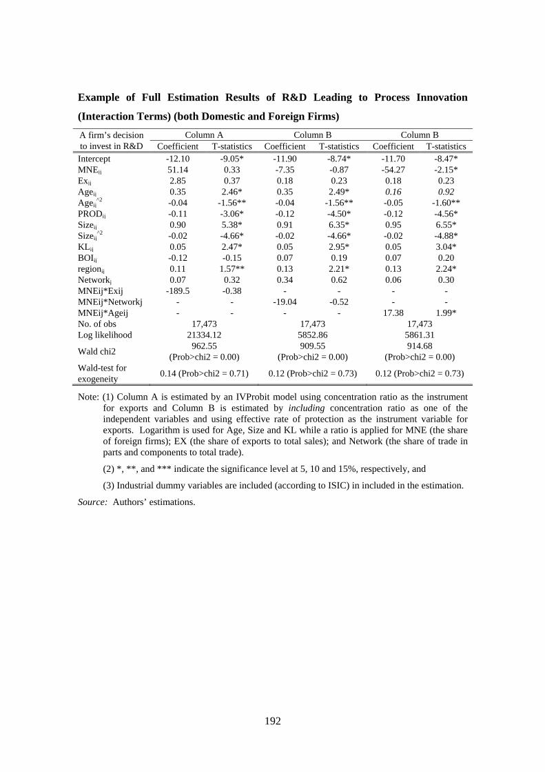
192  

Example of Full Estimation Results of R&D Leading to Process Innovation

(Interaction Terms) (both Domestic and Foreign Firms)

A firm’s decision to invest in R&D

Column A Column B Column B Coefficient T-statistics Coefficient T-statistics Coefficient T-statistics

Intercept -12.10 -9.05* -11.90 -8.74* -11.70 -8.47* MNEij 51.14 0.33 -7.35 -0.87 -54.27 -2.15* Exij 2.85 0.37 0.18 0.23 0.18 0.23 Ageij 0.35 2.46* 0.35 2.49* 0.16 0.92 Ageij

^2 -0.04 -1.56** -0.04 -1.56** -0.05 -1.60** PRODij -0.11 -3.06* -0.12 -4.50* -0.12 -4.56* Sizeij 0.90 5.38* 0.91 6.35* 0.95 6.55* Sizeij

^2 -0.02 -4.66* -0.02 -4.66* -0.02 -4.88* KLij 0.05 2.47* 0.05 2.95* 0.05 3.04* BOIij -0.12 -0.15 0.07 0.19 0.07 0.20 regionij 0.11 1.57** 0.13 2.21* 0.13 2.24* Networkj 0.07 0.32 0.34 0.62 0.06 0.30 MNEij*Exij -189.5 -0.38 - - - - MNEij*Networkj - - -19.04 -0.52 - - MNEij*Ageij - - - - 17.38 1.99* No. of obs 17,473 17,473 17,473 Log likelihood 21334.12 5852.86 5861.31

Wald chi2 962.55

(Prob>chi2 = 0.00) 909.55

(Prob>chi2 = 0.00) 914.68

(Prob>chi2 = 0.00) Wald-test for exogeneity

0.14 (Prob>chi2 = 0.71) 0.12 (Prob>chi2 = 0.73) 0.12 (Prob>chi2 = 0.73)

Note: (1) Column A is estimated by an IVProbit model using concentration ratio as the instrument for exports and Column B is estimated by including concentration ratio as one of the independent variables and using effective rate of protection as the instrument variable for exports. Logarithm is used for Age, Size and KL while a ratio is applied for MNE (the share of foreign firms); EX (the share of exports to total sales); and Network (the share of trade in parts and components to total trade).

(2) *, **, and *** indicate the significance level at 5, 10 and 15%, respectively, and

(3) Industrial dummy variables are included (according to ISIC) in included in the estimation.

Source: Authors’ estimations.

193

CHAPTER 6

Globalization and Innovation in Indonesia:

Evidence from Micro-Data on Medium and Large

Manufacturing Establishments

ARI KUNCORO

University of Indonesia

In this paper we examine the impact of globalization on innovation in the Indonesian

manufacturing sector. The lack of innovation data in the manufacturing survey has necessitated the

use of R&D expenditure as an input in the innovation production function. Globalization is

represented by being exporters, FDI and effective rate of protection (EPR). The model is set up such

that within the concept of R&D as conditional input demand function, allowing labor productivity to

have impact on R&D. In this case we find that less productive firms are less likely to venture into

R&D activities. In terms of globalization variables we find that being exporters is important

determinant of R&D. Meanwhile the impact of FDI firms on domestic R&D is only on the incidence

not on the intensity of R&D. It will require a critical mass of firm within a location or an

agglomeration to have a meaningful impact. Also lower ERP would induce firms to spend more on

R&D. So lowering protection or trade barriers will have positive impact on R&D.

Keywords: Indonesian manufacturing, Research and Development

JEL Classification: D21, O31, O12

194

1. Introduction

Globalization is a process whereby countries become more integrated via

movements of goods, capital, labor and ideas (Bloom, 2002). From the economic

policy standpoint, how globalization is transmitted into the domestic economy is

manifested in many ways, but is usually focused in the realm of trade and investment

liberalization. Decreasing trade barriers allow increasing exchange of goods and

services between countries. This process is facilitated by advances in information and

communication technology. In this setting new ideas are quickly brought to fruition and

new technologies are developed and superseded faster than at any other time in history.

More important than any other time in the past, knowledge has now become an

increasingly important determinant of the wealth of nations.

The importance of knowledge has revived attention on innovation systems and

research institutions. The process of globalization has made innovation more important

than before - even poor countries can no longer neglect the development of innovation

systems. Innovation systems as creators, adaptors and disseminators of knowledge can

be used as a vital tool for developing countries to benefit from globalization.

Firms now have to compete domestically and internationally. A Fast changing

business environment is a fact of life that has to be faced by corporations in the

globalization. From the organizational standpoint it requires firms to adjust quickly

with changing market demand immediately and for this they need to innovate.

The purpose of this study is to examine the impact of globalization on innovation at

the firm level in the Indonesian large and medium manufacturing. This study, using the

Indonesian micro data on large and medium size manufacturing establishment, attempts

to provide contribution to resolve the debate whether globalization is innovation

enhancing or innovation reducing. The key question is whether government policies to

liberalize trade and investment regime will boost innovations. If that the case then the

policy to open up the economy to global competition is desirable. It will allow

developing countries or more specifically Indonesia to jump up the learning curve by

bypassing the expensive process of invention. The government then after a series of

195

trade and investment liberalization policies could focus on policies to facilitate firms to

exploit the benefits of globalization.

The relationship between globalization and innovation is a complex one. Increasing

imports and inward foreign direct investment (FDI) brought about by decreasing trade

barriers would intensify competition in the domestic market and erode the domestic

firms’ profitability. This would force domestic firms to produce efficiently (Berthschek

, 1995). One way of staying competitive in business one way is to increase innovation

activity. So globalization and innovation may be positively related.

On the other hand, others have argued that the above relationship may be just the

opposite (Braga and Wilmore, 1991). Because firms have to spend handsomely on

R&D to create new product and new production processes while its return is highly

uncertain, they tend to be very conservative on innovation - focusing only on the

assimilation of imported technology to local conditions. Hence, the relationship

between globalization and innovation may be negative.

Between these two opposing views some prefer to adopt the middle ground stance

that globalization allows developing countries to jump up the learning curve without

having to undergo the lengthy and expensive process of discovery, by accessing ideas

and technologies developed elsewhere and putting them into practice after some

modification (Bloom, 2002).

Although the term “globalization” is well understood, translating it into more

‘operational’ variables for an empirical exercise is another matter. First globalization

can be considered as a regime change from a relatively highly regulated and protected

economy to a more open and deregulated one. Any economic reform that involves trade

and/or investment liberalization will suit into this definition. In this respect, the period

of analysis will be divided into before and after liberalization to examine the impact of

regime change on any defined outcomes, for example its impact on the number of

innovations conducted by firms.

The second way is more microeconomic in nature (i.e. at the firm or industry level).

As a result of the dismantling trade barriers, a firm has options to enter export markets,

operating as FDI, licensing or some or all combinations of the above. This applies to all

firms irrespective of their countries of origin (Bertschek, 1995). One implication is that

export activities, the presence of FDI and/or licensing can be used to signify the extent

196

of globalization at the firm, industry and national levels – depending on how

disaggregated is the analysis. One example is to use the ratio of exported output at the

firm level (Kuncoro, 2002). Meanwhile the presence of FDI firms is often used to

capture the impact of globalization on firms (Kuncoro, 2007). Therefore globalization

is treated as an exogenous factor – the possibility that firms learn through R&D to

become more productive so that they can go global as in Damijan et al. (2010), Crespi

et al. (2008) and MacGarvie (2006) is completely abstracted from.

For innovation the measurement is more straightforward. There are two aspects of

innovations, namely product technology or product innovation and process technology

or process innovation. Product innovation is a substantial improvement of a current

product or development and manufacture of a new product. Kraemer and Dedrick

(2000) for example, used the number of new products introduced over the last three

years to capture product innovation. Process innovation on the other hand involves

substantially improved or new production process through the introduction of new

process equipment or re-engineering of operational process. For example if a firm in a

specific period of time do the following; to set up new production line, to put in new

production system and to put in new computerized system to upgrade production

facilities, then they can be categorized as undertaking process innovation. This also

applies to the purchase of new capital equipment if it involves new production process

or at least brings improvement in production process.

The concept of ‘knowledge’ production function allows us to estimate directly the

determinants of innovation provided that the data are available. One important feature

of innovation data is that they consist of integer number and zero counts. This

necessitates the modification of distributional assumption when it comes to estimate

innovation function. The simplest is the Poisson distribution (Crepon and Duguet,

1997)

In subsequent development, Andersen (1970) extends the basic model to allow

estimation of fixed effects where the heterogeneity term ui is no longer assumed to be

independent of right hand side variables. So potentially one can allow individual or

industry effect such as different operating skills, appropriate condition and

197

technological opportunities in the innovation relationship.1 The pioneering work

applying the Poisson regression or count data model to the relationship between

innovation and R&D was conducted by Hausman et al. (1984).

One important contribution of this study is methodological – how to deal with the

situation when the innovation data are very rudimentary. Both types of innovation are

simply not available in BPS (Indonesian Statistical Agency) large and medium

manufacturing surveys. The only observed outcome from innovation activities is R&D

expenditure in which all product and process innovations are lumped together. To

overcome this problem instead using the knowledge production function directly, using

economic theory one can derive R&D expenditure as a product of the cost minimization

process where total cost of production which includes R&D expenditure is minimized

subject to a certain level of targeted output. In other words by relying on the concept of

innovation or the knowledge production function R&D expenditures are interpreted as

preceding activities prior to actual innovations. The attempt to endogenize R&D

decision is in line with Constantini and Melitz (2008) while export remains exogenous.

2. R&D Activities & Globalization in Indonesian Manufacturing

Before we proceed to the conceptual model guiding our empirical research, we

examine the main data sets – the annual survey of large and medium manufacturing

firms. The biggest problem is that the data do not contain the count of innovation, what

is available R&D expenditure. Under this condition, one way to get around the problem

is to model R&D expenditure as a conditional input-demand function representing

innovation generating activity.

The manufacturing data sets mentioned above are available from 1980 to 2007. So

potentially one can construct a long panel data to study the dynamic of R&D activities.

Unfortunately R&D expenditure is only recorded intermittently for the years 1995,

1996, 1997, 1999, 2000 and 2006. There is no R&D data prior to 1995.2 Although

1 This effect can be either fixed or random. 2 1996 was eventually dropped from our regression sample due to the fact that it misses one crucial variable for our modeling set up, namely new investment in machinery.

198

potentially one can construct a balanced panel data set, the main hurdle is to link data

sets before 2000 to that of 2006. We find that the firm identifiers are unreliable to link

the same firms from different years. So at best one can use the data sets in a pooled

fashion. Another problem is that R&D events are such rarities that from the total

combined sample from 1995 to 2006 the overall percentage of firms doing R&D rarely

exceeds 8 percent, which happened only in 1997 and 2006 (Table 1). On this

consideration, a lot more can be learned from firms’ decision to undertake R&D or not

by using a pooled sample.

Table 1. R&D versus no R&D

Year No R&D (%) R&D (%) Number of firms 1995 92.4 7.4 21530 1996 92.8 7.2 22969 1997 91.7 8.3 22355 1999 94.7 5.3 20445 2000 93.9 6.1 21762 2006 91.2 8.8 29421

Source: calculated from the Annual Manufacturing Surveys

Our observation on data sets will also help in determining the direction of the

modeling. In particular we want to know the main motivation behind carrying out

R&D. It is known that at the present stage of technology maturity, R&D has not been

an important factor in affecting the competitiveness (Kuncoro, 2002). Even if R&D

activities do exist, mostly they take the form of process innovation. Process innovation

involves substantially improved or new production process through the introduction of

new process equipment or re-engineering of operational process. There are three

situations where process innovation may take place: setting up a new production line,

putting in a new production system and installing new computer or information

technology components to upgrade production facilities (Kraemer and Dedrick, 2000).

The purchase of new capital equipment can be categorized as process innovation if

it involves a new production process or at least brings improvement in production

process. So a common occurrence is R&D activities taking place after new machinery

is installed. To examine this, we tabulate new machinery investment and the incidence

of R&D. The results are presented in Table 2.

199

Table 2. Firms Investing in New Machinery and R&D

Year

No New Machinery Investment New Investment in Machinery

% Firms doing R&D

Number of Firms % Firms doing

R&D Number of Firms

1995 5.4 18246 (84.7%) 19.6 3284 (15.3%) 1997 6.5 19401 (86.6%) 20.3 2954 (13.4%) 1999 3.5 17347 (85.2%) 15.1 3007 (14.8%) 2000 4.5 18622 (85.8%) 15.3 3100 (14.2%) 2006 5.6 25342 (86.1%) 10.4 4079 (13.9%)

Source: Calculated from the Annual Manufacturing Surveys.

For all years under observation firms making new investments in machinery have

higher likelihood of conducting R&D. In 1995 for example only 5.4 percent firms with

no new machinery investment carried out R&D. The corresponding figure for firm with

new machinery investment is almost four times higher. For both investing and non-

investing firms, the Asian economic crises have obviously had significant impact on

R&D activities. For investing firms the propensity to do R&D declined ever since and

it has yet recovered in 2006. On the contrary it reached its lowest figure of 10.4 percent

in that year. The figures for non investing firms are virtually flat – suggesting that there

is no relationship between R&D and machinery investment.3 The decision to invest in

new machinery is not an easy one. Since the investment cost is sunk a careful

consideration must be made by a firm taking account business uncertainty and future

profits, in effect it makes investment in machinery more volatile. Whatever the trend of

the likelihood of engaging R&D, Table 2 suggests that there is a relationship between

new investment in machinery and R&D.

As mentioned above, we hypothesize that an increase in competition from arising

globalization may induce firms to do more R&D. For this we replicate the above simple

analysis to two variables representing globalization, namely going into export market

and the presence of FDI firms (Table 3 and Table 4).

3 If there is no relationship between new machinery investment and R&D – the existence of R&D must be driven by something else like packaging, sales and so on.

200

Table 3. FDI Firms and R&D

Year

Non FDI Firms FDI Firms

% Firms doing R&D

Total Number of non FDI Firms

% Firms doing R&D

Total Number of FDI Firms

1995 7.1 20657 (95.9%) 18.6 873 (4.1%) 1996 6.7 21988 (95.7%) 18.7 980 (4.3%) 1997 6.7 21254 (95.1%) 20.9 1101 (4.9%) 1999 7.7 18926 (93.0%) 10.6 1428 (7.0%) 2000 4.8 20028 (92.0%) 13.1 1734 (8.0%) 2006 8.7 27252 (92.8%) 10.1 2169 (7.2%)

Source: Calculated from the Annual Manufacturing Surveys.

FDI firms are almost three times more likely to engage in R&D. In 1995 the

percentage of FDI firms recording R&D is 18.6 percent in contrast to 7.1 percent for

non FDI. The percentage of FDI firms carrying out R&D reaches its peak in 1997 just a

year before the Asian Crisis. As a mimic to observed pattern in the new machinery

investment before the likelihood of FDI firms engaging in R&D dropped after the

Asian crisis almost by half (Table 3). Interestingly the figures for non FDI firms show

a drop only in 2000 – the number is virtually stable for all other years. One plausible

explanation is that since R&D is tied to new machinery investment, the number is less

volatile for those that are less likely to make such investment namely non FDI firms.

Table 4 shows how exporting is related to R&D activities. Manufacturing is

dominated by non-exporters, which account for about 80 percent of total firms.

Exporting firms are clearly more likely to do R&D. But as in the previous analysis, the

likelihood to carry out R&D diminishes after the crisis and by 2006 it has still to

recover. To summarize there are three factors that may drive firms to engage in R&D:

making new machinery investment, being FDI enterprises and being exporters, all of

which may be interrelated. To disentangle this we have to wait for a formal

econometric analysis.

Table 4. Exporting Firms and R&D

Year

Non Exporters Exporters

% Firms doing R&D

Total Number of non-exporters

% Firms doing R&D

Total Number of Exporters

1995 6.1 17907 (83.2%) 15.1 3623 (13.0%) 1996 5.5 18614 (81.0%) 14.6 4354 (19.0%) 1997 7.3 19298 (86.3%) 14.8 3057 (13.7%) 1999 3.9 17553 (86.2%) 13.6 2801 (13.8%) 2000 4.3 18187 (83.6%) 13.0 3575 (16.4%) 2006 8.5 24422 (82.3%) 10.4 5199 (17.7%)

Source: Calculated from the Annual Manufacturing Surveys.

201

The above analysis yields the likelihood of firms to commit R&D but not the

propensity or intensity of doing so. To measure the propensity we use the ratio of R&D

expenditures to the values of total inputs, in percentage terms. The results are shown in

Table 5. All figures are quite small. None of them is higher than 1.5 percent.

Interestingly for all variables supposedly represent globalization namely; export

orientation and FDI, the results show that firms facing globalization do not necessarily

posses higher propensity to engage in RD. Globalization may increase the likelihood

or the incidence of R&D but it does not necessarily mean at high level.4 Higher levels

of R&D, regardless of denominator used may indicate sophistication so these small

values suggest that, if any, R&D activities may involve only non-sophisticated

activities. Another interesting observation is the observed turn around in 2006 where in

the categories of export orientation and FDI versus non FDI, all respective firms have a

higher propensity to engage in R&D compared to their non-exporter and/or non-FDI

counterparts, though all are at lower percentage. The Asian crises have lowered

propensity for R&D in all categories. The same pattern can also be observed for firms

with new machinery investment versus those without it.

Table 5. Percentage of R&D Expenditures to the Value of Total Inputs

Category Year

1995 2000 2006 Non Exporter 1.05 1.29 0..44

Exporters 0.88 0.87 0.70 No investment in new machinery 1.05 1.23 0.46

With investment in new machinery 0.90 0.92 0.65 No FDI firms 1.02 1.05 0.47

FDI firms 0.72 1.47 0.70 All firms 0.99 1.12 0.49

Source: Calculated from the Annual Manufacturing Surveys

R&D Intensity across Manufacturing Branches

The intensity to perform R&D certainly will differ from one industry to another. To

provide more detailed pictures across manufacturing we replicate the above observation

across two digits ISIC across manufacturing (Figure 1).

4 In our terminology the likelihood to engage in R&D irrespective of how much firms spend on it, while their propensity is the percentage of R&D expenditure to the value if inputs which indicates ‘level’.

202

Figure 1 0

.51

1.5

2P

erce

nt o

f RD

Exp

endi

ture

1995 2006

Percent of R&D to Input across Industries

31 32

33 3435 3637 38

Overall, the propensity to pursue R&D declined after the Asian crisis. Taking out

the outlier from paper (ISIC 34), both basic metal (ISIC 37) and machinery (ISIC 38)

have the highest R&D propensity. Still, the figures are low, for example in 2006 none

of them exceeds 1 percent. One plausible explanation is that R&D is a risky adventure

and the Asian crisis made firms more cautious. The other explanation links the R&D

decision to that of new machinery investment since most R&D is done in preparation of

installing new machinery/technology. With the same logic, since investing in new

machinery in the face of a sluggish economy in the aftermath of the Asian crisis is a

risky venture, R&D will also be affected.

203

Figure 2 0

12

34

Per

cent

of R

D E

xpen

ditu

re

1995 2006

31 32 33 34 35 36 37 38 39 31 32 33 34 35 36 37 38 39

Percent of R&D to Input across Industries

Exporter Non Exporter

Figure 2 divides the sample into the exporter and non-exporter categories. The

decrease of R&D propensity is also observed when comparing 1995 to 2006, but the

decrease for exporters is less than non-exporters. In 1995 non-exporters in food (ISIC

31), woods (ISIC 33), paper (ISIC 34), chemicals (ISIC 35) and basic metal (ISIC 39)

recorded higher R&D propensities. But the situation is reversed after the crisis. It

appears that in the face of increasing uncertainty, exporters facing competition abroad

have to maintain a minimum level or intensity of R&D expenditures which happens to

be higher than non-exporting firms, otherwise they would lose businesses. One

exception is heavily capital-intensive basic metal (ISIC 37) of which steel industry is

included. Even when the overall figures are declining between 1995 and 2006, non-

exporters have always higher R%D propensity.

204

Figure 3 0

12

34

Per

cent

of R

D E

xpen

ditu

re

1995 2006

31 32 33 34 35 36 37 38 39 31 32 33 34 35 36 37 38 39

Percent of R&D to Input across Industries: FDI vs Non FDI

FDI Non FDI

When comparing FDI versus non-FDI, there is no apparent consistent discernible

pattern (Figure 3). For example in 1995 for food (ISIC 31), woods (ISIC 33), paper

(ISIC 34), non-metallic (ISIC 36) and machinery (ISIC 38), the R&D propensity is

higher for non-FDI firms. This completely reverses in 2006. For the rest the pattern is

just the opposite. So the idea that being an FDI firm is a strong driver behind R&D is

not as convincing as the case of being exporters. But for this the final conclusion may

have to wait for a formal econometric test. In any case this pattern is useful in shaping

our conceptual model.

Next we turn to investment in machinery as a prime driver for R&D activities

(Figure 4). In 1995 the pattern is less clear, but in 2006 with basic metal (ISIC 37) as a

clear exception, in almost all other industries, machinery-investing firms tend to have a

higher R&D propensity. So in addition to a higher likelihood to engage in R&D (Table

2), the level of R&D expenditure is also relatively higher, which indicates a strong case

for new machinery investment as a primary reason behind R&D.

205

Figure 4 0

12

34

% o

f RD

Exp

end

iture

1995 2006

31 32 33 34 35 36 37 38 39 31 32 33 34 35 36 37 38 39

% of R&D Expenditures to Input

Fixed Capital Inv. No Fixed Capital Inv.

Effective Rate of Protection

One way for a government to shield certain sectors from global competition is

through tariff protection. This barrier will alter industry’s relative profitability by

creating an artificial price wedge. How the protection will affect R&D is at best

ambiguous. If the market is contestable then the extra profit can reinvested in R&D to

boost firms’ competitiveness in anticipation of the day when the protection is eventually

lifted. On the other hand, high artificial profits could also reduce pressure for firms to

carry out R&D. Both forces are present in a protected environment but which one is

stronger is a matter of empirical analysis.

To measure this we use the concept of the effective rate of protection (ERP) as in

Amiti and Konings (2005).

(1) )1(

)(kit

kt

kit

ktk

it

finputtariftarifferp

Where kit is the ratio of inputs to outputs for firm i in industry k at time t. A lower

output tariff would decrease the protection enjoyed by industry k, while a lower input

206

tariff would increase the protection received by industry k. To examine the possible

relationship between the R&D intensity and ERP, we compare the percent of R&D

expenditures in total inputs to ERP in figure 5.

Figure 5

0.5

11.

52

Per

cent

of R

D E

xpen

ditu

re

1995 2006

31 32 33 34 35 36 37 38 39 31 32 33 34 35 36 37 38 39

Percent of R&D versus ERP

mean of pirdvcu mean of erp

The overall pattern suggests that the percentage of R&D expenditure declined after

the Asian crisis. But one thing is obvious that higher ERP is associated with a lower

propensity conducting R&D. So dismantling of protection barrier has positive impact

on firms to do R&D to stay competitive. If R&D is tied to new machinery investment

then it is more likely directed to upgrade technology to boost competitiveness in the

face of increasing competition from abroad.

Information Spillover

Spatial centralization of resources and spatial concentration of manufacturing in a

few largest metropolitan areas has been a feature of the modern economy.

Centralization of industrial location at least in the early stages, may bring benefits to

207

firms (Hansen, 1990). One important benefit of such agglomeration is that firms

conducting R&D can learn from each other, to create a synergy that collectively boosts

their average productivity. In this regard there are two types of ‘positive’ externalities.

First is localization; in this respect firms doing R&D learn from their own industry,

which in the dynamic form, is often called Marshall-Arrow-Romer (MAR) externalities.

Alternatively, firms learn from all firms in a city, where the diversity of local industries

enhances the local information environment. This type of externalities is called

urbanization or in the dynamic context is termed Jacobs’ externalities (Jacobs, 1969).

In the Indonesian context, one important question is which type of externalities is

actually stronger for R&D. If externalities are in the form of localization, smaller city

are more likely to be the place of R&D activities specializing in just one industry or a

closely connected industries. On the other hand if the externalities happen to be

urbanization in nature, to thrive R&D activities need to find a location in a diverse and

large urban environment. R&D activities are therefore more likely to be found in large

urban areas. Another related question is whether externalities are mainly static or

dynamic. If it turns out that externalities are dynamic – this would imply that R&D past

activities affect the present productivity, because overtime a particular location would

accumulate a large body of knowledge. The implication for R&D is that firms

committing resources to do R&D would become more ‘static’ – tied to a particular

industrial agglomeration – and less willing to move to cities where historically R&D has

never existed, and thus have no built-up stock of knowledge.

Localization/MAR externalities will be measured by total employment in the own

industry in the respective districts. This measure is meant to capture interaction among

firms within a district. Urbanization externalities are measured by a diversity index.

For district i for example, the index of diversity is

(2)

2

1 )(

)(

)(

)(

tE

tE

tE

tEg j

i

ijJ

j

si

E(t) is total national manufacturing employment and Ej(t) is total national

employment in industry j. Meanwhile, Ei and Eij are the corresponding local

magnitudes. The measure of urbanization economies gsi(t) has a minimum value of

zero, where in a district, each industry’s share of local manufacturing employment is

208

exactly the same as its national share, so the district is completely unspecialized because

its industrial composition is merely a copy of the nation. At the other end, the

maximum value of gsi(t) will approach two for a district completely specialized in one

industry, while at the same time national employment is concentrated in another

industry. The higher is gsi(t) the lower is the diversity, thus a district becomes more

specialized.

To examine the location pattern of R&D activity we compare the percent of R&D

expenditure to the index of diversity given in (2) across industry. For easy comparison

we choose the year 1995 and 2006. The result is shown in Figure 6.

Figure 6

0.2

.4.6

.81

Per

cent

of R

D E

xpen

ditu

re

1995 2006

31 32 33 34 35 36 37 38 39 31 32 33 34 35 36 37 38 39

Percent of R&D versus Diversity Index

mean of pirdvcu mean of diversity

Although the pattern is somewhat less clear in 1995, the general relationship is that

an industry with a higher R&D percentage tends to locate in a location with a lower

diversity index or less specialized location, usually in bigger urban areas with bigger

more diversified economies. Since previously it has been asserted that most R&D are

directed toward preparation for new machinery investment (Figure 4), this type of R&D

209

may require only general information (capital goods markets, delivery times, general

specifications, after sales service and so on) from its industrial surrounding.

3. The Model

The conceptual model is developed in accordance of what was observed in the

background analysis that most R&D is presumably geared toward preparation for

incoming new machinery and equipment. It is also tailored to accommodate the fact

that the Indonesian manufacturing survey is at the establishment or plant level. A firm

before pursuing a risky R&D project will examine its long-run profits or cost

implications. From the economic theory we know that the existence of a duality

between profit and cost optimization would allow us to derive demand for factors of

production of which R&D is a crucial input.5

After an investment decision to improve machinery and equipment is made, the

necessary R&D activities are determined. For this, we rely on the concept of the

knowledge production function where R&D expenditure is related positively to

innovations (Crepon and Duguet, 1997) and the learning by doing model (Romer, 1996)

where innovations are learned from and are separable from the ongoing (constant

return) production process.

First we assume that there is a relation ship between innovation (n) and R&D

activities (R) in the following knowledge production function

(3) )(Rnn , where dn/dR>0 or a positive relationship exists between n and R.

Output, Y, is assumed to follow a general function

(4) ),,( nLKYY

where K is capital stock, L is labor and n are the number innovation. Substituting (3)

into (4) we have

(5) ),,( RLKYY

5 The conceptual model has undergone major revision in order to accommodate the suggestion that plant productivity should have an impact on R&D activities. Also the decision to carry out R&D has been restructured to account for concern that the choice model is not different from the location choice. Now the choice for R&D is treated more explicitly.

210

R&D is separable from the ongoing (constant return) production process. R&D is

modeled as a shift factor in the production function. If a firm chooses to carry out R&D

then it will add to its stock of knowledge B. By assuming a constant return to scale

technology for K and L in the production function, the appropriate form of this setup is

given by

(6) DRLKBY 1

With this specification the excess (super normal) profit function is defined by

(7) *. YP

where * is reservation profit which is assumed to be affected by factors that are

considered when choosing R&D projects such as the nature of the local agglomeration

including its industrial diversity (g) and own industry employment (e) which capture

technological information spillover as well as ERP) as a general measure of average

profitability.6 This also includes firm characteristics. R&D projects are risky

undertakings, to account for different degree of risk aversion among different types of

firm, firm characteristics such as being an exporter (ex) and/or an FDI are also

included.7

In (7) an increase of * would reduce Π so 0*

which would lower the

incentive to engage in R&D. Meanwhile the reservation profit is given by

(8) ),,,,(** fdiexERPeg

The relationship between * and ERP cannot be determined a priori, an artificial

increase of profitability because of higher protection may make firms ‘too lazy’ to

pursue R&D. In another case a foresighted firm may reinvest these profits in R&D in

anticipation that tariff barrier will come down in the future, so 0

ERP . The

relationship between the reservation profit and the nature of agglomeration (g and e) is

also ambiguous. It is up to the empirical exercise to determine the direction of these

relationships. Due to their outward orientation, exporters and FDI firms are presumably

6 So essentially excess profit is before labor, capital and material costs. 7 This will allow us to incorporate firm characteristics in the choice carrying out R&D project or not to represent different degree of risk aversion.

211

less risk-averse and thus have lower reservation profits compared to non-FDI and non-

exporters, so 0* ex and 0* fdi .

In equation (6) D is a dichotomous variable with the value of one if the excess or

super normal profit Π from undertaking an R&D project is greater or equal to zero or

Π≥0 and having the value of zero otherwise or if Π<0.8 If a firm chooses to undertake

an R&D project then the production process will follow

(9) )(1 BRLKY .

In (9) the impact of B and R on Y is given by the parameter θ, which is not constrained

so as to allow for decreasing, constant or increasing return of knowledge and R&D in

the production. If a firm opts not to purse R&D because of profitability or cost

concerns then the production will follow

(10) 1LKBY

which means a firm will use only the existing stock of knowledge. The per capita or

intensive form of (9) is given by

(11)

)()( BRkBRL

K

L

Yy

where y is output per unit of labor Y/L and k=(K/L) is capital-labor ratio. .

A firm will choose a level of R&D, R, as to optimize the capital and labor costs plus

R&D expenditure RwLrKC , with the excess normal profit Π≥0 as a constraint,

where r is price of capital and, w is wage rate. The conditional input demand function

for R&D is then given by

(12) )),,,,(,,( ** fdiexERPegL

YrRR

If a firm chooses to realize (12) by committing resources to perform R&D this is

because the excess normal profit requirement Π≥0 is met. Or alternatively it will not

spend on R&D if it is unprofitable or too costly or if Π<0. In this case there will be no

R&D activities or R = 0. In (12) r* is price capital normalized by wages w. In this

specification, y or Y/L can be interpreted as labor productivity so one can assess its

8 Compared to the earlier version, the choices are much simplified. Rather than having to choose one among many alternatives we now have a yes or no decision.

212

impact on R&D activities R, that is to say, whether firms with higher labor productivity

would have higher R&D intensity.

There is no specific ‘price’ for R to allow some flexibility of whether R&D is tied

to capital or labor. The property of strict concavity of (5) is sufficient to establish that

the negative relationship between r*=r/w and R in equation (9) does exist. Empirically,

this is a testable hypothesis which can be confronted with estimation results from the

data sets.9 Also the same property establishes positive relationship between R&D and

output per labor.

In (12) the impacts of being exporters and being an FDI firm on performing R&D

activities are given respectively by

(13) 0**

exex

R

and

(14) 0**

fdifdi

R

So being less risk-averse, exporters and FDI firms are more likely to engage in R&D.

The signs of other variables in (12) cannot be judged a priori – these will be determined

by the empirical models.

Instead of innovations per se we now have R&D expenditure as the crucial input in

the innovation process in the form of a conditional input-demand function.10 The

reservation profit π* incorporates globalization variables and other firm-industry

characteristics which will enable us to asses the impact of those variables on R&D and

indirectly on innovations employing their presumed correspondence suggested above.

The estimating version of equation (12) is therefore

(15) ititititititit uFGIL

Y

w

rR 3210 )()(

Where I is a dummy variable relating to whether a firm is investing in new

machinery/equipment or not, G and F are vectors of globalization and location-industry

level variables respectively. Variables representing G are being an exporter, being an 9 Interest rate r is calculated by dividing the amount of interest payment to total assets, while wages are constructed by dividing the total payroll for production workers with the total number of production workers. 10 Instead of observing the count of innovations, we look at innovation-generating activity, namely R&D.

213

FDI versus non-FDI and ERP.11 The vector F includes the diversity index g and own-

industry employment. Equation (15) can be estimated directly, lumping together all

variables affecting the decision to undertake R&D as well as the decision determining

R&D intensity. But if one wants to mimic a dichotomous choice i.e. to undertake R&D

or not depending on whether Π≥0 or Π<0, the Heckman procedure can also be used.

4. Empirical Results

The estimation results of equation (15) are shown in Table 6. In the first two

columns are the ordinary least squares method (OLS) applied to pooled data of the years

1995, 1997, 1999, 2000 and 2006. The difference between the first column and the

second is that in the latter all variables supposedly affecting the reservation profit π* are

included and also the ratio of interest rate to wages is replaced with a dummy ind

whether a firm committing new machinery investment or not as a direct test indicating

whether R&D activities are tied to machinery investment. Finally the last two columns

present the results of the two stage least squares – instrumental variables (2SLS-IV)

estimation. All standard errors are clustered in a respective district. By construction

output per labor in equation (11) is endogenous, thus output per labor in (12) and (15) is

also exogenous. For the instrument we use the district average of firms’ output.

Overall output per labor or labor productivity is positive and significant at least at

the 10 percent level so labor productivity is an important determinant in R&D activities.

In the model 1 of the OLS specification the coefficient of the ratio of interest rates to

wages is negative and significant at the 5 percent level.12 So there is an indication that

R&D is tied to the acquisition of capital goods. If the relative price of capital goes up

then it will have a negative impact not only on capital but also on R&D expenditures.

In model 1 the globalization variable is ERP is significant at the 5 percent level

though the coefficient is small. The sign is negative which implies that lowering

11 The exporter dummy is equal to one if a firm exports at least 2 percent its total output and zero otherwise. The FDI dummy is defined as equal to one if the share of foreign equity is at least 10 percent. 12 We experiment with the Tobit procedure but it is very weak statistically because not many firms are carrying out R&D.

214

protection would induce firms to increase R&D expenditure. The coefficients of other

globalization variables FDI and exporter dummies are positive, confirming the

prediction given by (13) and (14), and also significant albeit at different levels of which

the later is stronger statistically.

Turning to model 2 of the OLS specification, the most significant variable is the

new investment dummy – signifying that the most important factor behind R&D in

Indonesia is new investment in machinery and equipment. The exporter dummy retains

its significant but the FDI dummy is now insignificant. So being exporters have

stronger drive to carry out R&D compared to FDI firms.

Table 6. Determinants of R&D Expenditure: 1995-2006

Covariates OLS 2SLS

Model I Model II Model I Model II Output per labor 0.027 0.018 0.384 0.174 *[1.76] **[2.25] *[1.67] *[1.70] Ratio interest rate to wages -1.11 -0.376 **[-2.38] [-1.06] FDI Dummy 0.037 0.015 -0.032 -0.018 *[1..63] [1.10] [-0.58] [-0.57] Exporter Dummy 0.036 0.025 0.018 0.020 **[2.80] **[2.93] **[2.67] **[3.31] Effective Rate of Protection -0.00001 -0.00003 -0.00001 -0.00004 **[-2.99] [-1.25] [-0.83] [-1.21] New Investment in Machinery 0.043 0.036 **[3.34] **[3.71] Local Manufacturing Diversity -0.017 -0.012 (5 years Lag) **[-2.47] **[-1.99] Manufacturing Employment 0.000 0.000 (5 years lag) [-0.13] [-0.95] Industrial Dummies Yes Yes Yes Yes Time Dummies Yes Yes Yes Yes F-value **3.29 **10.26 Wald Chi-Square **55.09 **73.14 Number of Observation 73706 73706 73706 73706 Notes: Figures in parentheses are-test. * : Significant at the 10 percent level. **: Significant at the 5 percent level.

The ERP variable presents both in the model 1 and model 2 as to reflect the

situation that it may not only represent long-run (reservation) profits but also affecting

day to day operation especially when it comes to determine the level of R&D. It turns

215

out that ERP is not significant in model 2. Its effect may be swept away by the presence

of the new investment dummy of which most machinery is imported from abroad. This

suggests that from all globalization variables in the model, the exporter dummy is the

most robust. It survives different specifications as well as different estimation

procedures.

The diversity index is negative and significant at the 5 percent level. R&D

activities are higher in less specialized agglomerations usually in big urban areas –

confirming the notion that most R&D activities require more general market

information rather than industry-specific knowledge. The lag of own industry

employment is not significant, suggesting that specialization of R&D activities in

smaller cities is not a common phenomenon. Since the diversity index is also in the

lagged form, these externalities are dynamic, so it is not easy to relocate the present

R&D activities to non urban locations where historically they do not exist.

In the 2SLS-IV specification, output per labor is statistically weaker but still

significant - reflecting the problem of finding good instruments with high predictive

power but orthogonal to the error terms. One interesting finding is that the coefficient

of labor productivity is now larger. The productivity effect on R&D is larger after the

endogenous output per labor is taken care of.

The ratio of interest rates to wages is insignificant now although the sign remains

negative as before. The exporter dummy is still significant (model 1 of 2SLS-IV) with a

little smaller coefficient. ERP is not significant now, confirming that as a globalization

variable ERP, like the FDI dummy is not as statistically robust as exporter dummy.

Selectivity of R&D Activities

In the Heckman procedure we estimate equation (11) explicitly acknowledging the

decision that has to be made by a firm concerning R&D – whether to undertake R&D or

not (incidence of R&D) and, if so, how much it is willing to spend on it (R&D

intensity). The results are presented in Table 7.

216

Table 7. Selectivity of R&D Activity: 1995-2006 (Heckman Procedure)

Covariates Model 1 Model 2

Continuous Selection Continuous Selection Output per labor 0.792 0.014 0.799 0.020 **[2.05] *[1.74] **[1.97] **[2.49] Ratio interest rate to wages -34.85 -25.81 [-1.28] [-1.14] FDI Dummy 0.008 0.105 0.010 0.088 [0.05] *[1.74] [0.07] **[2.14] Exporter Dummy 0.096 0.431 0.057 0.465 [1.43] **[11.97] [1.35] **[14.10] Effective Rate of Protection -0.0002 ] -0.0002 **[-2.21] *[-1.74] New Investment in Machinery 0.650 0.633 **[18.64] **[19.86] Local Manufacturing Diversity -0.403 -0.337 (5 years Lag) **[-2.40] **[-2.27] Manufacturing Employment 0.000 0.00001 (5 years lag) [0.83] **[3.00] Industrial Dummies Yes Yes Time Dummies Yes Yes Mill-ratio -0.073 -0.067 **[-5.86] **[-6.33] Wald Chi-Square **9.93 **57.68 Number of Observation 107138 107138 Notes: Figures in parentheses are-test. * : Significant at the 10 percent level. **: Significant at the 5 percent level.

In the selection (incidence of R&D) equation we include variables that affect

reservation profits π* such as a new machinery investment dummy, a diversity index,

own industry employment, and EPR, along with the usual FDI and exporter dummies

and output per labor. In the continuous equation the usual conditional input demand

function is used where output per labor and the ratio of interest rate to wages are the

main variables along with other control variables such as FDI and exporter dummies.

The inverse of Mill’s ratio is strongly significant in both models, which implies that

performing R&D is not a random event. There is self-selection for firms devoting

resources to R&D. The difference between model 1 and model 2 is that in the former it

does not have industry and time dummies. But so far the models are robust to the

inclusion or exclusion of industry and time fixed effects.

Fulfilling the requirement for the conditional input-demand function set up, output

per labor is significant in the continuous equation in both models. The ratio of interest

217

rate to wages, however, is not significant though the sign conforms with the theory

(negative). Neither of the exporter and the FDI dummies in the continuous equation is

significant, suggesting that once an R&D decision is made R&D intensity in the day to

day operation is not influenced by firm types. This is akin to short-run versus long run

investment. Since R&D is tied to sunk-capital so once it is made it will bring the

consequence of R&D spending before and presumably even after installation of the

machinery.

In the selection equation, the ratio of interest rate to wages is replaced by a dummy

of new machinery investment. The coefficient of output per labor is strongly significant

in both models. So firms with higher labor productivity have higher probability to

perform R&D.

Unlike in the continuous equation where they do not affect the level of R&D

expenditures, the likelihood of firms undertaking R&D is now strongly influenced by

whether or not they are FDI firms or exporters or not. The other globalization variable,

ERP, is negatively related to the probability of carrying out R&D, though statistically is

somewhat weaker than the exporter dummy.

The lag of the diversity index is statistically very strong and has a negative sign.

This suggests that R&D activities are more likely to be found in less specialized

agglomerations. The result for the lag of own industry employment is mixed. It is

insignificant in model 1 where the dummy for new machinery investment does not

appear. In model 2 it is significantly positive. Certainly there is some degree of co-

linearity between these two but it still within a tolerable limit.

The most significant variable so far is the dummy for new machinery investment

which signifies the most important motive behind commitment to R&D as asserted in

the background analysis.

Spillover of the FDI Presence on Domestic Firms’ R&D

It is asserted in the background analysis that the presence of FDI firms may have

little impact on R&D. In this section we pursue this issue a little further by explicitly

constructing a variable to capture FDI spillover. We experiment with two alternative

218

indicators.13 The first is the number of FDI firms in a particular location. In the second

experiment, a diversity index is constructed exclusively for FDI firms, and added to the

model in place of the number of FDI firms in a district. One after another, these

variables are then put as a covariate in the regression of the conditional input demand

function for R&D where the sample is exclusively restricted to non FDI firms. The

results of the application of the Heckman procedure for this sample of domestic firms

are shown in Table 8.

Table 8. Impact of the Presence of FDI Firms on Domestic Firms R&D (Heckman)

Covariates Model 1 Model 2

Continuous Selection Continuous Selection Output 0.002 0.0001 0.002 0.0001 **[1.94] **[3.27] **[1.94] **[3.05] Ratio interest rate to wages -19.18 -17.22 [-1.00] [-0.95] Exporter Dummy -0.021 0.495 -0.022 0.490 [-0.37] **[13.95] [-0.40] **[13.83] Effective Rate of Protection -0.0002 -0.0002 **[-0.62] [-0.37] New Investment in Machinery 0.637 0.634 **[18.96] **[19.15] The number of FDI firms in a district -0.001 0.001 [-1.03] [1.40] Local diversity index of FDI firms 0.088 **[2.67] Industrial Dummies Yes Yes Yes Yes Time Dummies Yes Yes Yes Yes Mill-ratio -0.063 -0.060 **[-2.59] **[-2.41] Wald Chi-Square **66.96 **69.16 Number of Observation 104347 104347 Notes: Figures in parentheses are-test. * : significant at the 10 percent level. **: significant at the 5 percent level.

Overall, the results are weaker than the full sample but they are still plausible

statistically. The results for the crucial variables validating the equation as a conditional

input-demand function, output per labor and the ratio of interest rates to wages are

mixed. The coefficient of output per labor is positive and significant at the 5 percent

13 We actually experiment with two other variables namely the share of value added of FDI firms and the share of FDI firms’ workers in a particular district but both results are weak statistically.

219

level. The ratio of interest rates to wages has the right negative sign but it is

insignificant. Obviously removing FDI firms from the sample weakens its statistical

power.

None of the variables representing the presence of FDI firms matters in the

continuous equation. In the selection equation only the diversity index of FDI firms is

significant with a positive coefficient. The higher the FDI diversity index, the more

specialized a location is with FDI firms from one particular industry. Only then will

FDI firms have impact on R&D. However, this impact is limited to the incidence of

R&D, but does not affect the intensity of the activities. The significance of this variable

suggests that there is a critical mass of FDI firms in a location or in an agglomeration

below which the impact of FDI firms, at least on the incidence of R&D at domestic

firms is very small.

In this case the avenue through which FDI firms impact domestic firms’ R&D could

be through the force of competition or workers’ movement in a locality or both. The

limited impact of FDI firms on domestic firms’ R&D can be explained by the

circumstance that most of the FDI firms’ R&D may have been performed in their home

countries. Machinery and equipment may also have been standardized throughout their

plants around the world, so not much specific information about capital goods

technology can be exploited by domestic firms to produce a significant technological

improvement.

Impact of R&D on Labor Productivity

The setting up of the model suggests that the causal relationship between R&D and

labor productivity is bi-directional. R&D is modeled as a conditional input demand

function from a constant-return production process which is estimated empirically. The

results confirm that where output per labor affects R&D positively. So firms with

higher labor productivity have higher R&D intensity. But by a construction, the

intensive form of the production function in (9) also makes the direction of relationship

to reverse. For this purpose we estimate (9) empirically. The results are presented in

Table 9.

220

Table 9. Determinants of (log) Output per Labor Unit: 1995-2006

Covariates OLS 2SLS

Model I Model II Model I Model II Log of Capital per Labor Unit 0.233 0.185 0.227 0.174 **[18.09] **[14.07] **[17.54] *[1.70] Log of R & D Expenditure 1.971 1.401 6.211 4.375 **[10.97] **[10.42] **[2.13] *[1.95] FDI Dummy 1.010 0.937 **[14.91] **[11.65] Exporter Dummy 0.603 0.567 **[13.53] **[11.00] Industrial Dummies No Yes No Yes Time Dummies No Yes No Yes Prob>F or Prob>Chi-Squared **0.000 **0.000 **0.000 **0.000 R-Squared 0.227 0.349 0.177 0.325 Number of Observation 75109 75109 75109 75109

Notes: Figures in parentheses are-test. * : Significant at the 10 percent level. **: Significant at the 5 percent level.

In the first two columns the model is estimated with and without controlling for

firm characteristics, industry and time dummies, ignoring the potential endogeneity of

R&D. In the last two columns the 2SLS procedure is applied to account for this

problem. For the instrument the district average of R&D expenditure is used. The

coefficient of (log) R&D is always positive and significant. The coefficient of (log)

R&D is positive, larger and always significant, though a little weak statistically when

2SLS specification is controlled for firm characteristics and industry-time dummies,

which implies that R&D activities drive firms to become more productive. Therefore,

the relationship between R&D and labor productivity is indeed bi-directional. The

coefficient of (log) capital labor ratio suggests that the output elasticity with respect to

capital is around 0.20.

5. Conclusion and Policy Relevance

In this paper we examine the impact of globalization on innovation in Indonesian

manufacturing. One important contribution of this study is its method in dealing with

221

the situation when the innovation data are very rudimentary. The lack of innovation

data in the manufacturing survey has necessitated the use of R&D expenditure as an

input in the innovation production function. Globalization is represented by being

exporters, being FDI firms and the effective rate of protection (EPR). One caveat in this

study is that globalization is treated as exogenous factor. The situation where firms can

learns through R&D to become more productive so that they can enter the global export

market is completely abstracted from and it is left for future research.

The model is set up such that within the concept of a conditional input demand

function where it allows labor productivity to have impact on R&D. In this case we

find that less productive firms are less likely to venture on R&D activities. The reverse

causality is also true; namely firms with higher R&D intensity tend to be more

productive.

In terms of globalization variables we find that being exporters is an important

determinant of R&D. However, the impact of FDI firms on domestic R&D is only on

the incidence but not on the intensity of R&D. It requires a critical mass of firms within

a location or an agglomeration to have a meaningful impact. But the main motivation to

engage in R&D is in preparation for the installation of new machinery and equipment.

Through this avenue the impact of globalization may come indirectly from the desire of

firms to remain competitive, by upgrading their machinery and equipment.

Also a lower ERP would induce firms to spend more on R&D. So lowering

protection or trade barriers and maintaining openness will have positive impact on

R&D. Despite the fact that trade barriers are trending downward many hurdles remains

which continue to inhibit the flows of trade and investment. Two most important

problems are the corruption and inefficiency of national customs and ports. The

“national single window policy” and the establishment of Corruption Eradication

Committee (KPK) would reduce corruption and bureaucratic inefficiency. But

improving ports’ efficiency would require substantial investment which cannot be done

by the private sector alone.

With regard to information spillover R&D activities are more likely to be found in

less specialized industrial or economic agglomerations presumably in larger and diverse

urban areas but not in smaller cities. This is consistent with the earlier finding that the

primary motivation for R&D in Indonesia is for adaptation, accommodation and perhaps

222

some modification of new machinery and equipment to meet operational conditions in

Indonesia, so the type of information needed is general and is not a specific to consumer

needs. One policy implication from this is to maximize the gains from the current

configuration of industrial agglomeration and minimizing the negative externalities by

improving the connectivity between agglomerations.

223

References

Amiti, M., and J. Konings (2005), “Trade Liberalization, Intermediate Inputs and Productivity: Evidence from Indonesia’, IMF Working Paper, no. 146.

Andersen, E.B. (1970), ‘Asymptotic Properties of Conditional Maximum Likelihood Estimators’, Journal of the Royal Statistical Society, vol. 32:283-301.

Bertscheck, I. (1995), ‘Product and Process Innovation as a Response to Increasing Imports and Direct Investment’, Journal of Industrial Economics, vol. 43(4): 341-357.

Bloom, David (2002), ‘Mastering Globalization: From Ideas to Action Higher Education Reform’, Unpublished paper.

Braga, H., and L. Willmore (1991), ‘Technological Imports and Technological Effort: An Analysis of Their Determinants in Brazilian Firms’, Journal of Industrial Economics, vol. 39(4):421-431.

Constatini, J.A., and M. Melitz (2008), ‘The Dynamic of Firm Level Adjustment to Trade Liberalization’, in E. Helpman, D. Marin and T. Verdier (eds), The Organization of Firms in a Global Economy. Harvard University Press, Cambridge, M.A.

Crepon, B, and E. Duguet (1997), ‘Estimating the Innovation Function from Patent Numbers: GMM on Count Panel Data’, Journal of Applied Economics, vol. 12(3):241-263.

Crespi, G., C. Criscuolo and J. Haskel (2008), ‘Productivity, Exporting and the Learning by Exporting Hypothesis: Direct Evidence from UK Firms’, Canadian Journal of Economics, vol. 41(2):619-637.

Damijan, J.P., C. Kosteve, and S. Polanec (2010), ‘From Innovation to Exporting or Vice Versa’, World Economy, 374-398.

Hansen, N. (1990), ‘Impacts of Small and Medium-sized Cities on Population Distribution: Issues and Responses’, Regional Development Dialogue, vol. 11:60-76.

Hausman, J., B.H. Hall and Z. Griliches (1984), ‘Econometric Models for Count Data with An Application to the Patents-R&D Relationship’, Econometrica, vol. 52(4):909-938.

Jacobs, J. (1969), The Economics of Cities. Random House, New York.

Kraemer, K.L and J.L. Dedrick (2000), ‘The Information Technology Sector and International Competitiveness: A Background Paper’, paper presented at the ADB Consultation Meeting, Asian Institute of Technology, Bangkok.

Kuncoro, A (2002), ‘International Trade, Productivity and Competitiveness’, in J.S. Fanelli and R. Medhora (eds), Finance and Competitiveness in Developing Countries, Routledge.

224

___________, (2007), ‘Manufacturing Growth in a Country Undergoing Political Transaction: How Firms Cope with Changing Business Environment in Indonesia’, paper presented at GDN Medal Competition, Beijing.

MacGarvie, M. (2006), ‘Do Firms Learn from International Trade’, Review of Economics and Statistics, vol. 88(1):46-60.

Romer, D. (1996), Advance Macroeconomics. McGraw-Hill, New York.

225

CHAPTER 7

Globalization, Innovation and Productivity in Manufacturing Firms:

A Study of Four Sectors of China

JACQUES MAIRESSE

INSEE-CREST (France), UNU-MERIT (Netherlands), and NBER (USA)

PIERRE MOHNEN UNU-MERIT (Netherlands), and Maastricht University

YANYUN ZHAO

Renmin University of China

FENG ZHEN1

Bank of China, and Chinese Academy of Social Science.

This paper investigates relationships between innovation input, innovation output and labor

productivity in China for four major manufacturing sectors; textiles, wearing apparel, transport

equipment and electronic equipment. It uses a large sample of firm level micro data and a structural

model in the estimation. The data from 2005 to 2006 is estimated, and results of all the sectors show

positive effects from innovation input to output, and then to firm performance. Globalization has

various impacts on innovation, through exports. It has a positive effect on both the decision to carry

out R&D, and intensity of R&D input in sectors with competitive advantage, such as textiles and

transport equipment, but not in sectors with high levels of overseas capital control, such as

electronic equipment and wearing apparel. Ownership reveals the same story in different sectors,

namely that foreign firms tend to do less in innovation input and output, but they do have higher

level of productivity. Moreover, market share, subsidy, firm size and other characters of firms are

involved in the estimation, which explains significant difference in engaging in innovation and

production. Thus, in all the sectors, market share improves R&D input, continuous R&D input and

exports improve new products output. Subsidy sustains R&D input, but not innovation output.

Keywords: R&D, New Product, Productivity, Export, CDM Model

JEL Classification: D21 L67 O31

1 Corresponding Author: Feng ZHEN, zhen@ruc.edu.cn. We would like to thank Chin Hee Hahn, Keiko Ito, Dionisius Narjoko, Shujiro Urata and other participants in the ERIA Workshops for the Microdata Project FY 2010 for their valuable comments and suggestions. We also appreciate the financial support of ERIA, Europe and China Co-ordination Research Fund (COREACH-64-094), and Feng thanks the China Postdoctoral Science Foundation (No.20100480239). The opinions expressed in this article are the authors’ and not necessarily those of the institutions.

226

1. Introduction

Innovation is a key concept in moving into the knowledge-based economy, not only

for the further development of developed economies such as the United States and

European countries, but also for the reform and development of China. During the

past thirty years of reform, China has achieved rapid growth and becomes a "world

factory". In the new century, China is seeking for a new development approach to

improve productivity, save energy and resources, but maintaining the fast pace of

development and aiming to be the world’s manufacturing center at the same time. The

most practicable strategy is to establish a knowledge-based economy and make

innovation a main factor in research and development, production and management,

especially in manufacturing sectors at the firm level. The macro data in Table 1 shows

the fast growth of R&D input and productivity in China during the past decade.

Nevertheless, the absolute amount, measured as R&D input in business, the rate of

R&D input in GDP, or GDP per capita, is still far less than in developed countries.

Industrial productivity in China is less than one sixth of the United States’ level in 2008

even at purchasing power parity (PPP), which is much higher than current values in

China.

Table 1. R&D Expenditure and Productivity across Countries

China India Germany Japan Korea USA

Total expenditure on R&D 1997 (% of GDP) 0.64 0.70 2.24 2.87 2.48 2.56

Total expenditure on R&D 2007 (% of GDP) 1.44 0.83 2.53 3.44 3.21 2.65

Business expenditure on R&D 1997 (% of GDP) 0.30 0.16 1.51 2.07 1.80 1.87

Business expenditure on R&D 2007 (% of GDP) 1.04 - 1.77 2.68 2.45 1.91

Business expenditure on R&D 1997 (USD Billion) 2.83 0.67 32.75 88.08 9.30 155.41

Business expenditure on R&D 2007 (USD Billion) 35.25 - 58.91 117.45 25.68 269.27

GDP per capita 1997 (USD) 771 437 26445 33776 11237 31038

GDP per capita 2007 (USD) 2560 965 40430 34262 21655 46680

Productivity in industry 2000 (PPP, USD) 8512 6349 57902 52086 35106 69507

Productivity in industry 2008 (PPP, USD) 18196 9656 84601 70709 64169 120118

Source: IMD, World Competitiveness Yearbook, online database.

227

Globalization has been regarded as a key to world development since the last

century, no matter whether people have positive or negative attitudes towards it. China

always shows an active attitude towards globalization by opening its market, especially

the manufacturing sector, encouraging foreign direct investment (FDI) and exports.

FDI has been encouraged, and has grown very quickly since the beginning of the reform

process. It has higher levels of management and efficiency in production, brings a

fresh atmosphere and new techniques, improves exports and helps the government gain

foreign exchange. Nowadays, FDI is an important element in the Chinese economy,

and it controls more than half of the firms in some key manufacturing sectors, especially

in electronics-related high-tech sectors. At the same time, growth of exports supports

the fast growth of the economy and helps the country obtain its reputation as “world

factory”. Table 2 shows the process of globalization. The Stock of incoming FDI has

started from 0.15% of the world’s total amount since the beginning of reform. It

reached 2% in 1993, the highest to 3.46% in 1997, and nearly the same level with

Canada in the first decade of this century. Export grew from less than 1% of the world

to 5% in 2002, and nearly 10% in 2009. GDP grew from 2.58% of the world in 1980

to 8.21% in 2009, but the per capita value is still less than 10% of United States’ level.

Table 2. Growth of FDI, Export and GDP in Mainland China

1980 1990 2000 2005 2006 2009

Foreign direct investment stock-Inward (% of the world)

0.15 0.99 2.60 2.36 2.05 2.67

Total merchandise trade-Export (% of the world)

0.89 1.78 3.86 7.25 7.99 9.68

GDP (% of the world) 2.58 1.82 3.72 5.07 5.65 8.22

GDP per capita (% of USA) 2.66 1.61 2.84 4.40 5.02 8.21

Source: United Nations, UNCTAD database.

In the new century, China’s development is focusing on sustainable development in

a fast growing economy, and the improvement of residents’ welfare. Innovation at the

firm level is a key step in improving productivity, sustaining the reform of industrial

structure and supporting manufacturing firms’ competition in the global market. That

is why the Sustainable Development Strategy and Innovation-oriented Country Strategy

of China came into being in 2006.

228

Based on a large sample of firm level data, this paper will investigate why firms

choose to carry out R&D, how R&D input supports new product output, how R&D

activity affects productivity, and the effect of globalization, e.g. FDI and exports, on

innovation during the process.

The paper focuses precisely on four major but distinctive manufacturing industries:

Textiles (code 17), Wearing Apparel (code 18), Transport Equipment (code 37) and

Electronic Equipment (code 40).2 The first two industries are more labor intensive and

low-tech, while the others are more capital intensive and high-tech. All four are not

only important in the Chinese domestic market but also in the world market. The

textile industry is the largest manufacturing sector in China, in terms of number of firms

and size of labor force. The textiles and wearing apparel industries, are sectors with

competitive advantages in the world market and but also are sectors in which trade

conflicts can easily arise. Furthermore, these sectors have sufficient power to

influence the employment market in China, and the textile products market worldwide.

The transport equipment sector has been a developed industry for more than half a

century in China, and it will grow fast with the high-speed railway plan in Mainland

China in the coming decades. More than half of the electronic equipment firms are

controlled by overseas capital, which makes it a sector with two foreign markets:

materials and components imported from abroad and products exported abroad,

especially to developed countries. All the four sectors have grown extremely quickly

and have been quite innovative in recent years. Our analysis thus relies on four firm

samples separately for the 2 years: 2005-2006.

The paper is organized as follows. Section 2 summarizes the literature strands.

Section 3 introduces the equations of the structural model and the estimation method of

this paper. Section 4 describes data and variables selection. The empirical results are

presented in section 5 and section 6 draws the conclusion and policy suggestions.

2 Electronic Equipment here means “Manufacture of Communication Equipment, Computers and Other Electronic Equipment”. It is comparable with code 32 in UN ISIC 3.1.

229

2. Literature Review

The productivity ratio between input and output in production has been a classical

area of study since the Cobb-Douglas production function was proposed in 1928.

Since then, thousands of discussions, ameliorations and empirical studies have been

contributed to this academic area, together with the remarkable improvements by

Tinbergen (1942), Solow (1957), and Jorgenson (1987). Griliches (1979) develops the

knowledge production function and gives innovation criteria a new position in the

equation. Crépon Duguet and Mairesse (1998) propose a new system, combining the

innovation selection function, the knowledge production function and the production

function together to analyze the innovation procedure and production performance.

That is what we call the CDM model.

The CDM model is a systematic attempt to understand the relationships and

linkages among innovation input, innovation output and production performance,

especially using firm level data. Most of the existing studies using a CDM model

incorporate survey data, especially Community Innovation Surveys (CIS) data from

European countries.3 Lööf and Heshmati (2002) study Swedish CIS II data to analyze

knowledge capital and firm performance. They give a good comparison of key

parameters in earlier CDM models. The parameters are various but all are positive

using French and Swedish data. Janz et al. (2004) compare innovation and productivity

in Germany and Sweden by using CIS III firm data and get "a common story across

countries". Ferreira et al. (2007) give both separate and simultaneous estimation of a

CDM equations system and get different results by using Portuguese CIS II firm data.

Mohnen et al. (2006) work on CIS I firm data to compare 7 European countries and

develop the measure of innovativity, which combines the micro measurement and

aggregate macro comparison. Benavente (2002) estimates the CDM model by using

Chilean survey data designed under the reference of CIS, but the sample size is much

smaller.

3 Up to 2010, Eurostat has launched five innovation surveys under the direction of the "Oslo Manual". These surveys are known as CIS I to CIS V, mainly organized in 1993, 1997-1998, 2000-2001, 2004, and around 2010.

230

A CDM related model has been estimated in a few papers using hard data, including

data from China.4 Jefferson et al. (2006) studies R&D and firm performance of

Chinese large and medium-size manufacturing firms by using a rich set of census data

from 1997 to 1999, with original observations of nearly 20,000 in all manufacturing

sectors before being cleaned each year.5 Hu and Jefferson (2004) discuss the same

question using sample survey data of state-owned enterprises located in Beijing.

These results suggest substantial and significant returns to R&D, and a difference across

industries.

Export and FDI based globalization is another interesting topic discussed in

academic papers. Empirical study of the linkage between exporting and innovation

using micro data has increased in recent years. One direction emphasizes the

contribution of innovation to entry into the global market. Most of the results suggest

a positive effect of innovation on exports, e.g. among Canadian manufacturing firms by

Baldwin and Gu (2004), German service firms by Ebling and Janz (1999), and Chinese

firms by Guan and Ma (2003).6 Another is the reverse direction; i.e. investigating the

causality from exports to innovation, i.e. the learning-by-exporting effect in firms. A

positive impact of exporting on innovation at the firm level is presented in Salomon and

Shaver (2005) for Spain, Hahn (2010) for Korea, and Tsou et al. (2008) for Taiwan.

Moreover, Amiti and Freund (2008) find that China’s export growth is supported by

growth of existing products, rather than new products, Wang and Wei (2008) find that

foreign firms do not conduct R&D to introduce new products.

This paper will focus on firm behavior, from the innovation process to firm

performance. Effects of exporting and foreign ownership on innovation are

investigated during the stepwise estimation. The contribution of this study is the

subdivided sector level study which tests the effectiveness of the CDM model by not

4 Hard data means not survey data where standard answers are selected, but real amounts of value in accounting and production, such as the value of exports, sales of new products and so on. 5 The size is defined by the China National Bureau of Statistics. The standards are different among sectors using particular products, fixed assets and so on before 2002. The system was simplified in 2003 using three criteria i.e. labor force, sales of products and total assets, but most of them can be compared with the old standards. Here are the new standards for reference: medium-size manufacturing firms' must have at least 300 people, 30 million sales and 40 million assets; large-size must have 2000 people, 300 million sales and 400 million assets. 6 Other inconsistent results by Willmore (1992), Sterlacchini (2001) and other papers suggest the contrary, though the amount is much smaller than the positive results.

231

using survey, but firm level hard data, and distinguishes the globalization effect on

innovation.

3. Econometric Model

The CDM model gives us a systematic understanding of the innovation path in

production. It brings together the three main fields of investigation in the

econometrics of research and innovation, i.e. why firms select innovation inputs,

innovation output efficiency, and innovation’s impact on productivity. It has three

steps and four equations written as follows, with i index firms and t index year. Vector

x series are explanatory variables, vector b series are parameters and vector u

series are error terms.

Innovation input: ( 1) 0( 1) 0 0t i t i ibrd x b u

(1)

1( 1) 1 1( 1) t i it ilrdpl x b u

(2)

Innovation output: 2 2 2( 1)

*ti it iti lrdpllnppl x b u

(3)

Innovation performance: 3 3 3

* ti ti iti lnppllp x b u (4)

Step one, known as the innovation function, explains innovation input with two

equations shown as equations (1) and (2). The first equation is a probit model as a

selection equation to understand firms' decisions about whether or not to input

innovation. The second equation is a Tobit model to explain why they would like to

spend more or less on innovation. We use the Heckman procedure in the STATA

software to estimate the first two equations, in which the data is one year earlier than the

following two steps.7 Explained variables in innovation input are measured by a

binary variable (brd) in the probit model to identify whether firms have made an

7 The result for electronic equipment is difficult to converge by using data of 2005. We use the pooled 2005-06 data in all the 3 steps after comparing the 2006-only result.

232

innovation input or not, and R&D intensity measured by R&D expenses per labor unit

(lrdpl, in logarithm) in the Tobit model to explain why they would choose to spend

different amounts on innovation. The regressors are market share, capital intensity,

binaries of exporting and subsidy, as well as control variables such as firm size

dummies and ownership dummies.8

Step two with equation (3) is a knowledge production function, proposed by

Griliches (1979), which explains innovation input and its influence on innovation

output. Innovation output is measured by new product output per labor unit (lnppl, in

logarithm) to identify the extent to which firms have innovation output. Here we

estimate its predicted value (lnppl) and input it as an explained variable in the third step,

so that all the firms can be involved in the last equation. The predictor variables are

predicted value of R&D expenses (lrdpl), capital intensity, a binary of export and

subsidy, and dummy groups of firm size and ownership.

In the first two steps, we test an innovation related group of binary variables, export

and subsidy, to explain the relative characters of globalization and government support

for firms’ innovation behavior.

Step 3 with equation (4) is an extended Cobb-Douglas production function to

explain innovation output and its influence on productivity, measured by labor

productivity (lp, in logarithm). The predicted value of innovation output (lnppl) is a

regressor, except for the traditional variables of capital intensity and number of

employees. Dummy variables for ownership, as well as region and sub-sector are also

added in this step.

In order to include all the firms in the model, we follow the estimation method in

Griffith et al. (2006) by using predicted values from earlier steps in later steps. Some

groups of variables are added as binaries or dummies to specify characters of firms,

such as ownership, region, size, sub-sector and so on. We also estimate the innovation

input equation one year earlier than the innovation output and firm performance

8 “Subsidy” which is the income from government or international organizations, involves 3 main kinds. The first is innovation related income, e.g. subsidy for carrying out an R&D project or filing a patent, obtaining a development fund, or producing some special kinds of new products. The second is production related, e.g. return of added value tax for exports, subsidy for environment protection. The third is income of obtaining an award, e.g. bonus for pilot products, famous brand award and so on. Appendix Table A2 lists the average labor productivity of firms with or without subsidy. We will not discuss the table further due to the complex components of this variable.

233

equations, assuming that innovation input has a time lag in influencing innovation

output, but the effect of innovation output on performance is mainly in the same year.

Similarly, we estimate the pooled four sectors to test the robustness of our findings.

The estimation using estimated values assumes that all firms have the potential for

innovation. This is a simplification of the original CDM model, which is much more

convenient than the other two methods. One of these is the simultaneous estimation of

four equations using the Inversed Mills Ratio, estimated in the earlier step, to correct the

standard error. The other is to give zero observations, especially those in innovation

variables, a very small value like 0.0001 to avoid selectivity bias (Jefferson et al., 2006).

4. Data and Description

4.1. Data and Selection

This paper will use the industrial census data in 2005 and 2006.9 They are the

most recent firm level data that it is possible to obtain from the China National Bureau

of Statistics. It is a yearly census of all state-owned firms, and those non-state-owned

middle and large firms above a designated size.10 The criteria are all hard data and

most of them are from yearly accounting reports by enterprises. The structure of the

data is similar to but much richer than Jefferson et al. (2006) investigate, for the textile

sector observations alone reach 20,000 before “cleaning” in 2006. The dataset gives

us a wide field of research, but also poses challenges in terms of variances and other

matters which require sector by sector investigation.

From the original data we delete those firms with fewer than 10 employees, or

whose sales of products are less than RMB 5 million, or whose value added is less then

zero.11 Then we calculate the growth rates of sales, labor and capital for each firm.

9 We do have a long panel before 2005, but there is a gap of observation changes and an unexpected absence of innovation criteria in 2004, which restricts the usage of the long run panel. 10 The designated size means that Sales of Products is higher than RMB 5 million (about EUR550,000). Firms larger than this size are included in the census scheme and report their data every year by filling in a set of statistical forms. Firms smaller than this size are surveyed separately using sampling methods. 11 The deletion of small sales firms can help us to get the same standard of state-owned and non-state-owned firms, since non-state-owned firms with sales less then 5 million are not included in the census scheme.

234

Firms with all the three growth rates between the 2.5 and 97.5 percentile are kept in the

modeling. Thus we obtain two-year balanced data from 2005 to 2006.

Three groups of variables are selected to establish the CDM model. The first

group are basic variables in innovation and the production function, including labor

productivity calculated as value added divided by number of employees, number of

employees, capital (shown as net value of fixed assets) per employee, all in logarithm.12

The second group is innovation variables, with R&D expenses per labor unit (in

logarithm), new products output per labor unit(in logarithm) and a binary to identify

whether the firm has continuous R&D expenses or not in 2006, following its positive

expenditure in 2005. The third group is extended variables including market size,

measured by sales ratio in 3-digit sub-sectors, firm size by four dummies, categories of

capital control by five ownership dummies to measure the ownership of each firm. All

these variables are detailed in appendix A.13

4.2. Basic Description

Table 3 gives the basic description of variables in each sector and each

corresponding year, with the pooled four sectors data in the last two columns for

reference. For basic variables, average labor productivity increases more than 15% in

textiles and transport equipment in 2006, about 10% in wearing apparel, but only 3.5%

in electronic equipment, though this sector has the highest level of productivity. The

average numbers of employees are around 300, 340 and 350 in the first three sectors

respectively, and they do not change much across the two years. The number is much

higher in electronic equipment firms, and it grows about 10% in 2006 to nearly 700

people. Capital intensity in wearing apparel is about 23,000 RMB, much lower than

that of the other three sectors, whose intensity is about 70,000 to 80,000 RMB.

12 Capital per employee is also a predicted variable used in the innovation function to measure firm size, together with market size. 13 It is the smallest sector category in China Industry Standard. The market size defined as sales

ratio like: ln( / )it it itsub sector

lsts S S

, with itS index sales of products of firm i in year t, and

itsub sector

S index of total sales of the 3-digit sub-sector that firm i involved in in year t. Each firm

belongs to only one 3-digit sub-sector in the database. We do not have further information about different products in one firm.

235

Table 3. Means of Variables across Sectors and Years

Textile Wearing Apparel Transport Equipment Electronic Equipment

Pooled 4 Sectors

2006 2005 2006 2005 2006 2005 2006 2005 2006 2005

Basic*

Productivity 80.3 68.7 50.2 45.7 104.1 90.0 117.8 113.9 84.0 74.6

Labor 307 303 342 333 362 355 684 622 382 367

Capital per Employee

67.7

64.3 23.4 22.5 74.2 70.7 80.8 80.2 61.2 58.8

Innovation

R&D * 2.5 1.5 1.7 1.9 10.1 8.5 18.3 16.9 11.0 9.7

R&D>0 0.062 0.057 0.048 0.047 0.215 0.192 0.281 0.251 0.121 0.110

Continuous R&D 0.035 - 0.025 - 0.148 - 0.202 - 0.080 -

New Product * 75.5 62.3 102.1 86.2 514.2 421.7 790.6 707.0 456.6 368.6

New Product>0 0.083 0.072 0.061 0.067 0.180 0.164 0.196 0.181 0.114 0.105

Dummy Variables

Export=1 0.403 0.408 0.645 0.645 0.279 0.269 0.585 0.579 0.459 0.459

Subsidy=1 0.140 0.154 0.115 0.120 0.187 0.182 0.192 0.193 0.152 0.158

Firm Size

Size:<50 0.128 0.130 0.033 0.032 0.110 0.116 0.082 0.085 0.097 0.099

Size:50-99 0.237 0.238 0.139 0.138 0.251 0.267 0.173 0.185 0.208 0.214

Size:100-249 0.350 0.349 0.401 0.407 0.345 0.341 0.287 0.283 0.350 0.350

Size:250-999 0.234 0.231 0.379 0.379 0.226 0.210 0.308 0.303 0.275 0.270

Size:>999 0.052 0.052 0.049 0.044 0.068 0.065 0.150 0.144 0.069 0.066

Ownership

State-owned 0.009 0.010 0.006 0.006 0.049 0.052 0.018 0.018 0.018 0.018

Limited Liability

0.111 0.111 0.077 0.073 0.194 0.190 0.129 0.119 0.122 0.119

Share-holding 0.014 0.015 0.009 0.010 0.024 0.025 0.023 0.024 0.016 0.017

Private 0.586 0.575 0.422 0.414 0.426 0.415 0.252 0.251 0.469 0.460

HMT 0.135 0.134 0.239 0.238 0.081 0.078 0.261 0.259 0.166 0.165

Foreign 0.098 0.098 0.210 0.214 0.130 0.131 0.286 0.295 0.157 0.159

Number of Firms 13245 6645 5926 4534 30350

Notes: (1) The table lists the balance panel data by year. (2) Variables with "*" are original variables before logarithm, with the units of RMB000 in

current prices, except labor which is headcount. Price is adjusted in the regression. The indices of the 4 sectors in 2006 are 102.1, 100.9, 99.5, and 96.6, respectively.

(3) R&D is the average R&D expense per employee of firms with R&D>0. (4)New Product is the average new product output per employee of firms with New

Product>0. (5)HMT means Hong Kong, Macao and Taiwan.

For innovation variables, only about 5% to 6% of firms have R&D input in the first

two low-tech sectors. This grows to about 20% in transport equipment, and nearly

236

30% in electronic equipment. In all these four sectors, for those firms with R&D input

in 2005, more than half of them continue to input in innovation in the second year.

This proportion is 77% in transport equipment and 80% in electronic equipment.

Furthermore, R&D intensity is quite different among these sectors. Textile and

wearing apparel firms have about 2,000 RMB R&D expenses per employee in those two

years, while the number in transport equipment is about 10,000, and 18,000 in

electronic equipment. The R&D expenses increase in three sectors and decrease in

wearing apparel, but it is difficult to describe a long-term trend for the two-year data.

For innovation output, the proportion of firms outputting new products firms is about

1% to 2% higher than the R&D input ratio in the two low-tech sectors, but is lower in

the two high-tech sectors, especially about 7% to 8% lower in electronic equipment.

The estimation result will explain why input is lower but output is higher in this sector.

The intensity of new products output in all the sectors grows fast in 2006, though the

average level is quite different among these sectors. High-tech sectors have much

higher new product output than low-tech. This reaches 790,000 RMB in electronic

equipment and 514,000 RMB in transport equipment. It is only around 100,000 RMB

in wearing apparel, but this is higher than that in textiles.

The ratios of firms which export are about 40% in textiles, 64.5% in wearing

apparel, and around 58% in electronic equipment. The export ratio is much lower in

transport equipment, reaching only around 27% of all the firms in this sector. The

ratio of firms receiving subsidy is higher in the high-tech sectors than in the low-tech

sectors. Nearly 20% of high-tech firms have subsidy from the government, either for

innovation or export. Only about 15% of textile firms and 12% of wearing apparel

firms receive any subsidy from the government. The trend of this ratio goes slightly

down in 2006 for all the sectors except transport equipment.

Firm size dummies show significant increases in the two smallest categories and

decreases in the two largest categories in all these sectors. Ownership dummies show

private firms are the largest ownership group in the first three sectors, comprising

around 58% of textile firms, about 42% of wearing apparel firms and the same

proportion in transport equipment firms. Overseas capital, including Hong Kong,

Macao and Taiwan (HMT) and foreign capital, controls more than half of electronic

equipment firms. Moreover, state-owned firms are a very small proportion in all these

237

four sectors: 5% in transport equipment, and less than 2% in the other three sectors.

Together with Limited Liability Corporations and Share-holding Corporations, firms

controlled by state or public capital are less than 20% in all the sectors, except about

27% in transport equipment.

4.3. Innovation and Export in Firm Performance

Table 4 presents labor productivity in different innovation and/or export

aggregations. In all these sectors, the productivity of R&D innovators is much higher

than non-R&D innovators, and that of product innovators is much higher than non-

product innovators in almost all cases, whether or not the firm is an exporter. For

instance, the average productivity of innovators among electronic equipment firms is

46% larger than that of non-innovators in 2006, and 40% in 2005. The only exception

is product innovators in wearing apparel, with 13% lower productivity than non-

innovators in 2005. On the other hand, levels of productivity specifies by export are

quite different among sectors. Non-exporters always have higher productivity than

exporters in most cases in the low-tech sectors, but the productivity of exporters is

higher than non-exporters in most cases in the high-tech sectors. The only two

exceptions are textile product innovators in both years and non-product innovators in

electronic equipment in 2006. Comparing these two methods of classifications, the

difference between exporters and non-exporters is much smaller than that between

innovators and non-innovators.

Table 4. Cross-table of Labor Productivity

Textile

Wearing Apparel

Transport Equipment Electronic Equipment

2006 2005 2006 2005 2006 2005 2006 2005

All firms 80.3 68.7 50.2 45.7 104.1 90.0 117.8 113.9

of which: Exporter 72.8 62.8 47.0 42.0 113.4 95.4 121.7 120.5

Non-Exporter 85.4 72.8 56.1 52.5 100.5 88.0 112.4 104.9

R&D Innovator 95.0 80.3 70.2 62.4 133.0 116.2 158.6 143.2

of which: Exporter 92.3 80.1 63.9 58.5 139.3 120.5 167.6 148.0

Non-Exporter 98.3 80.6 80.9 68.7 128.2 113.4 145.1 136.2

Non-R&D Innovator 79.4 68.0 49.2 44.9 96.2 83.8 102.0 104.1

of which: Exporter 71.0 61.4 46.1 41.3 100.7 85.5 103.2 111.0

Non-Exporter 84.8 72.4 54.8 51.6 94.8 83.3 100.3 94.7

238

Table 4 (continued). Cross-table of Labor Productivity

Textile

Wearing Apparel

Transport Equipment Electronic Equipment

2006 2005 2006 2005 2006 2005 2006 2005

Product Innovator 90.0 72.3 49.2 38.6 123.8 106.6 163.8 158.0

of which: Exporter 95.1 73.4 46.8 35.7 130.9 110.5 176.6 165.5

Non-Exporter 77.4 69.4 59.8 49.9 115.9 102.7 139.0 145.1

Non-Product Innovator 79.4 68.4 50.3 46.3 99.8 86.8 106.7 104.2

of which: Exporter 69.0 61.3 47.0 42.6 104.4 88.9 106.2 109.4

Non-Exporter 85.7 72.9 56.0 52.6 98.5 86.1 107.3 97.3

Notes: (1) The table lists the average value of balance panel data by year. (2) The unit is RMB000 in current prices. (3) Numbers of firms are omitted. The 3 smallest groups have 76, 89, and 118 firms.

5. Empirical Result

Empirical results of the CDM model help to answer the following questions, (i) why

or why not the firms decided to engage in R&D input, and what is their reason for

expending more or less in innovation if they decided to spend at all, (ii) whether

innovation output is the result of R&D input or not, (iii) whether firms’ innovation

output improves their product output performance, and (iv) the effect of globalization

variables, such as exporting and ownership, on innovation.

The results can be interpreted in two dimensions: the equation and variable level,

and the sector level. The equation level tells us the main relationships of the

innovation process, globalization and firm performance by the parameters of key

variables. The sector level may tell a different story in different industries when they

practice innovation. We will follow the equation level to organize the discussion.

5.1. Innovation Input

We start the interpretation by considering why and to what extent firms choose to

innovate. The eight columns in Table 5 give estimates of the four selected sectors, and

compare selection and intensity equations sector by sector. The innovation input

equations show that firms’ capital intensity and market share are significantly positive in

improving R&D input for all the four sectors, in both selection and intensity equations,

239

in 2005. They are extremely similar among sectors and between selection and

intensity equations.

Table 5. Innovation Input: Selection and Intensity Equation

Textile Wearing Apparel

Dep. Var.= R&D Selection Intensity Selection Intensity

(1) (2) (3) (4)

Market Share 0.109*** 0.349*** 0.130*** 0.271**

(0.017) (0.071) (0.021) (0.119)

Capital per Employee 0.109*** 0.510*** 0.137*** 0.251**

(0.018) (0.074) (0.028) (0.123)

Export 0.120*** 0.327* -0.059 -0.291

(0.041) (0.171) (0.060) (0.216)

Subsidy 0.223*** 0.633*** 0.318*** 0.732**

(0.046) (0.186) (0.073) (0.329)

Size:50-99 0.181*** - 0.115 -

(0.071) (0.179)

Size:100-249 0.211*** - 0.116 -

(0.069) (0.171)

Size:250-999 0.448*** - 0.202 -

(0.072) (0.171)

Size:>999 0.772*** - 0.376* -

(0.091) (0.205)

State-owned 0.146 -0.498 0.808*** -1.008

(0.154) (0.540) (0.219) (0.779)

Limited Liability 0.126** -0.043 -0.039 -0.070

(0.056) (0.214) (0.103) (0.366)

Share-holding 0.234** -0.097 0.018 1.089*

(0.120) (0.413) (0.216) (0.655)

HMT -0.280*** -1.110*** -0.302*** -0.241

(0.063) (0.261) (0.077) (0.323)

Foreign -0.115* -0.509* -0.254*** -0.253

(0.066) (0.262) (0.078) (0.306)

Constant -1.394 -4.125 -0.904 -1.924

(0.205) (0.727) (0.293) (1.192)

Rho 0.825 0.660

(0.040) (0.229)

Wald 95.56 28.05

Log Likelihood -4053.9 -1773.9

Observation 12982 6645

Note: Year=2005.

240

Table 5(continued). Innovation Input: Selection and Intensity Equation

Transport Equipment Electronic Equipment

Dep. Var.= R&D Selection Intensity Selection Intensity

(5) (6) (7) (8)

Market Share 0.039*** 0.194*** 0.156*** 0.196***

(0.014) (0.036) (0.014) (0.042)

Capital per Employee 0.236*** 0.574*** 0.070*** 0.227***

(0.021) (0.067) (0.013) (0.038)

Export 0.060 0.110 0.010 -0.656***

(0.050) (0.126) (0.037) (0.098)

Subsidy 0.289*** 0.129 0.663*** 0.731***

(0.050) (0.129) (0.036) (0.151)

Size:50-99 0.265*** - 0.007 -

(0.092) (0.068)

Size:100-249 0.519*** - -0.002 -

(0.088) (0.070)

Size:250-999 0.982*** - 0.060 -

(0.093) (0.084)

Size:>999 1.493*** - 0.228** -

(0.120) (0.104)

State-owned 0.402*** -0.326 0.710*** -0.216

(0.089) (0.223) (0.108) (0.272)

Limited Liability 0.330*** 0.195 0.478*** 0.623***

(0.055) (0.165) (0.049) (0.154)

Share-holding 0.307** 0.562** 0.602*** 0.686***

(0.121) (0.277) (0.100) (0.225)

HMT -0.199** -0.415* -0.352*** -0.633***

(0.086) (0.251) (0.047) (0.149)

Foreign 0.102 0.287 -0.363*** 0.074

(0.067) (0.178) (0.046) (0.146)

Constant -2.222 -1.471 0.372 1.191

(0.187) (0.466) (0.180) (0.343)

Rho 0.370 0.322

(0.086) (0.119)

Wald 136.88 159.88

Log Likelihood -4634.2 -9673.5

Observation 5926 9068

Note: Year=2005 for Transport Equipment, but pooled 2005 & 2006 for Electronic Equipment.

241

Export parameters are significantly positive in textiles and negative in electronic

equipment, but are not significant in the other two sectors. Textiles is a traditional

sector with a world competitive advantage that may encourage firms to decide to

undertake R&D so as to keep their advantage, and the high profits from potential

markets, by spending more on innovation. Transport equipment firms have the same

ownership structure as textiles and some degree of advantage in the world market,

which supports the positive but not significant coefficients in both equations. The

opposite is true in electronic equipment; that is, a small positive but not significant

coefficient is shown in choosing to innovate, but a large negative coefficient appears in

the intensity equation, which means that the more firms export, the lower their level of

R&D intensity. The result is partly because of the high proportion of overseas capital

control in this sector. They pay more attention to exports, but do not necessarily do

much research work since most of this kind of work has been done, or even the key

component elements have been finished in foreign institutes and factories. A high

level of globalization in this high-tech sector is a kind of product globalization, but not a

globalization of research activity. Wearing apparel shows the same story, with large

negative coefficients of export due to the similar ownership structure, and design work

done abroad in exporting firms.

In all these four sectors, firms with subsidies choose to carry out R&D and the

subsidy helps to improve R&D intensity. The parameters in all the equations show

significantly positive effects, except only one positive but not significant coefficient in

the intensity equation for transport equipment.

Firm size dummies suggest that larger firms tend to choose to carry out R&D, the

same as suggested by market share. The parameters quickly go up in textiles and

transport equipment, while the largest group of firms in the other two sectors have

significantly positive effects.

Ownership dummies tell a common story in all the sectors, and we specially

emphasize the effect in electronic equipment since the rule is especially clear in it.

Compared with private domestic firms, firms controlled by overseas capital especially

firms controlled from Hong Kong, Macao and Taiwan (HMT firms), tend not to

undertake R&D, or to input less if they do. Firms controlled by state or public capital

tend to carry out more R&D. This is a similar result to that derived from our earlier

242

research, and we can get further explanation in the following steps. We can also obtain

a successfully positive test in part of the Schumpeter hypothesis, by parameters of either

market share or firm size. That is, large firms have a higher tendency towards

innovation selection and innovation input.

5.2. Innovation Output

The knowledge production function in table 6 shows that predicted R&D expenses

were significantly positive in improving innovation output in 2006. The marginal

effects are similar (about 0.15 to 0.20) in the first three sectors, and up to 0.84 in

electronic equipment. And if firms continue to do R&D in the second year, they will

produce more new products.

Table 6. Innovation Output: Knowledge Production Function

Dep. Var.= New Product Textile Wearing Apparel Transport Equipment Electronic Equipment

(1) (2) (3) (4)

R&D_hat 0.152*** 0.190** 0.156* 0.844***

(0.049) (0.081) (0.082) (0.097)

Continuous R&D 0.996*** 1.110*** 0.914*** 0.528***

(0.075) (0.123) (0.060) (0.050)

Capital per Employee 0.059* -0.040 0.036 -0.103***

(0.035) (0.037) (0.055) (0.032)

Export 0.641*** 0.360*** 0.611*** 0.959***

(0.047) (0.071) (0.056) (0.075)

Subsidy 0.084 -0.062 0.106* -0.306***

(0.052) (0.088) (0.056) (0.083)

Size:50-99 0.052 -0.067 0.018 -0.182**

(0.073) (0.174) (0.098) (0.073)

Size:100-249 0.005 -0.129 0.091 -0.166**

(0.073) (0.165) (0.095) (0.071)

Size:250-999 0.178** 0.020 0.414*** -0.236***

(0.082) (0.167) (0.104) (0.080)

Size:>999 0.506*** 0.050 0.719*** -0.220**

(0.112) (0.205) (0.139) (0.104)

State-owned 0.476*** Dropped 0.159 0.427***

(0.166) (0.116) (0.125)

243

Table 6 (continued). Innovation Output: Knowledge Production Function

Dep. Var.= New Product Textile Wearing Apparel Transport Equipment Electronic Equipment

(1) (2) (3) (4)

Limited Liability 0.148** -0.150 0.065 -0.129

(0.059) (0.108) (0.063) (0.083) Share-holding 0.363*** -0.210 0.096 -0.117

(0.130) (0.265) (0.145) (0.129) HMT -0.009 -0.197** -0.095 0.147*

(0.080) (0.080) (0.108) (0.082) Foreign -0.064 0.027 -0.294*** -0.463***

(0.073) (0.078) (0.088) (0.057)

Constant -0.980 -0.511 -1.081 -0.255

(0.412) (0.444) (0.449) (0.164)

Pseudo R^2 0.2899 0.1838 0.3065 0.2333

Log Likelihood -2638.3 -1240.5 -1935.1 -3343.5

Observation 12962 6514 5892 9046

Notes: (1) Year=2006 for the first 3 sectors, but 2005 & 2006 pooled data for Electronic Equipment. (2) R&D_hat is the estimated result in the innovation input equation, with 1 year lag to the

innovation output equation, except the same year in the Electronic Equipment sector.

Export improves innovation output in all the sectors, which suggests that firms

serving the global market tend to engage in producing new products, whether or not

they themselves choose to undertake R&D.

Subsidy only significantly impacts innovation output in the two high-tech sectors,

but in opposite directions. It is positive in transport equipment, but negative in

electronic equipment since firms in the latter sector gain new products not by doing

subsidy supported R&D, but more often by directly using technology transferred from

abroad. Furthermore, domestic firms in the electronic equipment sector with low

levels of output tend to obtain a variety of support from government in the name of

innovation, since this sector has been defined as a core high-tech sector, and emphasized

by the government as an area to be encouraged in innovation policy. Foreign firms get

less in subsidy, but they hold their competitive advantage by using technology from

abroad, which can sufficiently support the high efficiency of their product innovation.

On the other hand, the insignificant coefficients in low sectors indicate two things.

The first is that low-tech sectors like textiles and wearing apparel obtain subsidies for

exporting to a greater extent than from innovation. The second is that the government

pays more attention to the linkage of innovation and high-tech business, but ignores the

244

importance of innovation in keeping a competitive advantage for those low-tech sectors

that have already found global competitiveness.

Firms size dummies tell the same story of the importance of size in the first three

sectors, supporting the opinion that large firms tend to have more new product output.

On the other hand, large electronic equipment firms tend to have low new product

intensity. Ownership in all the four sectors indicates that firms controlled by state or

public capital have a high intensity of innovation output and firms controlled by

overseas capital have less. Comparing with the R&D input equations in the first step,

we get common results in ownership dummies, and similar results in at least three

sectors except for electronic equipment in innovation output.

5.3. Innovation Performance

Finally, we interpret the firm performance estimation of the production equation as

shown in Table 7. The parameters of estimated new product output in all four sectors

give a positive effect. The elasticity of each sector is from 0.246 in transport

equipment, to 1.112 in electronic equipment.

Table 7. Innovation Performance: Production Function

Dep. Var.= Productivity Textile

Wearing Apparel

Transport Equipment

Electronic Equipment

(1) (2) (3) (4)

Capital per Employee 0.209*** 0.188*** 0.233*** 0.125***

(0.007) (0.010) (0.012) (0.009)

Labor -0.300) -0.214*** -0.188*** -0.294***

(0.008) (0.013) (0.015) (0.010)

New Product_hat 0.354*** 0.467*** 0.246*** 1.119***

(0.017) (0.040) (0.026) (0.029)

State-owned -0.646*** Dropped -0.427*** -0.683***

(0.090) (0.059) (0.084)

Limited Liability -0.118*** 0.060 -0.068** -0.386***

(0.024) (0.038) (0.028) (0.033)

Share-holding -0.215*** 0.242** 0.026 -0.439***

(0.069) (0.104) (0.077) (0.067)

245

Table 7 (continued). Innovation Performance: Production Function

Dep. Var.= Productivity Textile

Wearing Apparel

Transport Equipment

Electronic Equipment

(1) (2) (3) (4)

HMT 0.037* 0.054** 0.029 0.258***

(0.021) (0.025) (0.043) (0.026)

Foreign 0.058** -0.033 0.351*** 0.453***

(0.023) (0.024) (0.038) (0.028)

Constant 4.964 4.607 4.289 5.535

(0.071) (0.108) (0.163) (0.091)

F 96.86 46.70 40.71 103.32

R^2 0.2913 0.1803 0.2927 0.3979

Observation 12962 6514 5892 9046

Notes: (1) Year=2006 for the first 3 sectors, but 2005 & 2006 pooled data for Electronic Equipment.

(2) Region dummies and sub-sector dummies are estimated, but omitted in the table.

In contrast with the results of the R&D input equations and new product output

equations, the results for firm performance are quite different for the ownership

dummies. Compared with private domestic firms, firms controlled by overseas capital

tend to have higher productivity, though they input less in R&D terms, and produce

fewer new products. On the other hand, firms controlled by state and public capital

tend to have lower productivity, though they are apt to carry out R&D and have more

new products. According to this point, one advantage of globalization is that the

competition among firms in the global market leads to a positive effect on productivity

growth in mainland China.

5.4. Globalization and Innovation

Comparing coefficients of the exports and foreign ownership dummies in the first

two steps, the globalization of Chinese manufacturing sectors tells the following story.

Exports and foreign markets are not necessarily the causation for R&D. It depends on

whether the sector has a technological advantage controlled domestically or from

abroad. The domestic control tends to improve performance and market growth by

innovation, whilst the foreign control tends to finish the R&D and core technical work

abroad and to perform only the manufacturing step in mainland China. Neither high-

tech nor low-tech decides the high R&D effort. Sectors with local technology control,

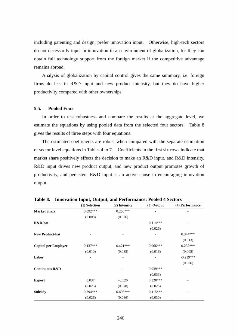
246

including patenting and design, prefer innovation input. Otherwise, high-tech sectors

do not necessarily input in innovation in an environment of globalization, for they can

obtain full technology support from the foreign market if the competitive advantage

remains abroad.

Analysis of globalization by capital control gives the same summary, i.e. foreign

firms do less in R&D input and new product intensity, but they do have higher

productivity compared with other ownerships.

5.5. Pooled Four

In order to test robustness and compare the results at the aggregate level, we

estimate the equations by using pooled data from the selected four sectors. Table 8

gives the results of three steps with four equations.

The estimated coefficients are robust when compared with the separate estimation

of sector level equations in Tables 4 to 7. Coefficients in the first six rows indicate that

market share positively effects the decision to make an R&D input, and R&D intensity,

R&D input drives new product output, and new product output promotes growth of

productivity, and persistent R&D input is an active cause in encouraging innovation

output.

Table 8. Innovation Input, Output, and Performance: Pooled 4 Sectors (1) Selection (2) Intensity (3) Output (4) Performance

Market Share 0.092*** 0.250*** - -

(0.008) (0.026)

R&D-hat - - 0.114*** -

(0.026)

New Product-hat - - - 0.344***

(0.013)

Capital per Employee 0.137*** 0.421*** 0.066*** 0.237***

(0.010) (0.035) (0.016) (0.005)

Labor - - - -0.219***

(0.006)

Continuous R&D - - 0.939*** -

(0.033)

Export 0.037 -0.126 0.528*** -

(0.025) (0.078) (0.026)

Subsidy 0.394*** 0.696*** 0.115*** -

(0.026) (0.086) (0.030)

247

Table 8 (continued). Innovation Input, Output, and Performance: Pooled 4 Sectors

(1) Selection (2) Intensity (3) Output (4) Performance

Size:50-99 0.157*** - -0.015 -

(0.045) (0.047)

Size:100-249 0.247*** - 0.018 -

(0.044) (0.045)

Size:250-999 0.475*** - 0.207*** -

(0.046) (0.048)

Size:>999 0.736*** - 0.394*** -

(0.056) (0.060)

State-owned 0.479*** -0.198 0.198*** -0.460***

(0.062) (0.174) (0.073) (0.043)

Collective 0.266*** 0.256** 0.175*** -0.106***

(0.031) (0.104) (0.034) (0.016)

Corporate 0.389*** 0.685*** 0.306*** -0.029

(0.066) (0.180) (0.075) (0.043)

HMT -0.303*** -0.798*** -0.136*** 0.001

(0.035) (0.121) (0.042) (0.014)

Foreign -0.178*** -0.123 -0.185*** 0.136***

(0.033) (0.108) (0.036) (0.014)

Constant -1.688 -3.017 -1.402 4.419

(0.105) (0.325) (0.158) (0.050)

Rho 0.626

(0.038)

Wald 646.30

F 270.21

R^2 / Pseudo R^2 0.2678 0.2777

Log Likelihood -15335.7 -7831.9

Observation 30087 30074 30074

Notes: Region dummies and sector dummies are estimated and significant, but omitted in the table.

In contrast to the various coefficients’ direction of export in the separate four

sectors, the aggregate estimation interprets that export to the global market does not

significantly impact R&D input, but the overseas market demand does improve new

product output.

Without the individual sector characteristics, subsidy retains positive significance in

the first two steps using aggregate data, which suggests that subsidy is an important

element in supporting the R&D input decision, innovation intensity and new product

248

output. In addition, the effect might be varied in the different sectors that have been

investigated in the former sections.

Size dummies indicate that large firms tend to make R&D input, and they also have

a higher level of new product output intensity. Ownership dummies give the same

result as before, namely that firms controlled by state and public capital have the

contrary situation in innovation and productivity, compared with firms controlled by

overseas capital. Firms controlled by state and public capital tend to undertake R&D,

and they have a higher level of R&D intensity and new product output, but their

productivity is lower than private domestic firms. However, firms controlled by

overseas capital tend to do less in innovation, but they have a higher productivity,

compared with private domestic firms.

6. Conclusion and Policy Remarks

By using a separately estimated CDM model, this paper investigates innovation

behavior, and its ability to promote productivity in four Chinese manufacturing sectors.

All “cleaned” firms are involved in the model by using predicted values of innovative

variables in the estimation of the first two steps. Only four selected sectors are used in

this paper due to the complex census data, but they do give sufficient results in different

industries, as well as distinguishing the effects of exporting, subsidy, and ownership.

Moreover, the results from pooled data sustain the robustness of the sector level

estimations.

We conclude the paper by discussing four outcomes, which also indicate the

directions for relative policy recommendation.

The main result is that the model proves the positive effect of innovation input on

innovation output, and on innovation output on productivity. It sustains the national

innovation strategy of improving innovation input in research and development,

especially at the firm level. Firm level innovation input is the key element in

improving labor productivity, and the foundation of welfare-based wealth accumulation.

249

The second outcome is that exporting improves innovation output, but does not

always sustain innovation input. The innovation output efficiency depends on the

demands of the global market through exports, and the innovation input depends not on

exports, but on the competitive advantage of the sector in the world market. Therefore

creating a competitive advantage in technology is as important as, or even more

important than the advantage derived from exporting. The policy towards FDI should

encourage not only foreign capital growth and foreign-owned manufacturing processes,

but also technology transfer and the spillover of innovation. Besides exporting,

customers’ demand drives product innovation, which suggests that the exploration of the

domestic market is another important means of promoting local R&D, especially for

such a large market as mainland China. These are the key processes of the coming

economic structure transformation in China.

The third outcome is the interesting opposite effect of different ownerships in

innovation and productivity. Firms controlled by state and public capital innovate

more due to their operation of the whole process of local production, though they tend

to have low levels of productivity. Firms controlled by overseas capital innovate less

but produce more, due to their lack of local R&D input, but transfer technology from

abroad. In addition, native firms are sensitive to the influence of the government’s

innovation policies, but private firms controlled by overseas capital make their decision

on innovation more simply, related to higher profits or lower taxes. The better way to

encourage innovation is to open more and gives the decision to the firms, so that they

can evaluate changes of the market through competition. The policy of encouragement

of firms based on ownership criteria should be weakened, and the government should

pay more attention to the construction of a fair market and competition environment.

For the above two conclusions, globalization is conducive to creating added value

and to sustaining years of fast growth through exports and FDI. Moreover, the next

step is to learn more from globalization, to establish a better environment of innovation

by strengthening the protection of intellectual property rights, transferring policies from

encouraging capital introduction to encouraging local innovation in an impartial market

environment during the long term of sustainable development.

The last outcome is that innovation is effective not only in high-tech, but also low-

tech sectors. Innovation has a positive effect in low-tech sectors such as textiles,

250

which have already gained competitive advantage in long-term development through

globalization. Innovation policy should pay more attention to encouraging R&D in

this kind of sector, which is important for the maintenance of its competitiveness and for

sustaining its employment.

Given the limitations of our work, and in particular to our using only 2 years’ data

from 4 selected sectors, these initial results should be merely taken as illustrative. We

pay more attention to R&D and new product innovation rather than to exports in the

systematic estimation, and leave a wide area for further investigation based on the large

sample of firm level accounting data. One interesting field is the decomposition of

productivity growth by R&D, exports, and FDI. Another is the specification of

relationships between innovation and exports, the two key words in the Chinese

economy. We will carry out further work in the rich mine of micro data.

251

References

Amiti, Mary and Caroline Freund, (2008), “The Anatomy of China’s Export Growth’, World Bank Working Paper, No.4628.

Baldwin, J.R. and W. Gu, (2004), “Trade Liberalization: Export-Market Participation, Productivity Growth, and innovation’, Oxford Review of Economic Policy, 20(3):372-392.

Benavente, J. M., (2002), ‘The role of Research and Innovation in Promoting Productivity in Chile’, mimeo.

Crépon, B., E. Duguet, and J. Mairesse, (1998), ‘Research and Development, Innovation and Productivity: An Econometric Analysis at the Firm Level’, Economics of Innovation and New Technology, 7(2), 115-158.

Ebling Gunther and Norbert Janz, (1999), ‘Export and Innovation Activities in the German Service sector: Empirical Evidence at the Firm Level’, ZEW Discussion Paper, No.99-53.

Ferreira Lopes, Luísa and Manuel Mira Godinho, (2007), ‘Innovation and Productivity in Services: An Empirical Micro Study’, DRUID Working Paper, No. 05-08.

Griffith, R., E. Huergo, J. Mairesse, and B. Peters, (2006), ‘Innovation and Productivity across Four European Countries’, Oxford Review of Economic Policy, 22(4), 483-498.

Griliches, Z., (1979), ‘Issues in Assessing the Contribution of Research and Development to Productivity Growth’, Bell Journal of Economics, 10(1), pp.92-116.

Guan, J and Ma, N., (2003), ‘Innovative Capability and Export Performance of Chinese Firms’, Technovation, 23(9), 737-747.

Hahn, Chin Hee, (2010), ‘Does Exporting Promote New Product Introduction: Evidence from Plant-Product Data on Korean Manufacturing’, FREIT Working Paper , No.100112.

Hu, A. and G. Jefferson, (2004), ‘Returns to Research and Development in Chinese Industry: Evidence from state-owned enterprises in Beijing’, China Economic Review, (15) 86-107.

Janz, N., H. Lööf, and B. Peters, (2004), ‘Firm Level Innovation and Productivity – Is There a Common Story across Countries’, Problems and Perspectives in Management, (2) 184-204.

Jefferson G., B. Huamao, G. Xiaojing and Y. Xiaoyun, (2006), ‘R and D Performance in Chinese Industry’, Economics of Innovation and New Technology, 15(4/5), pp.345-366.

Lööf, H. and A. Heshmati, (2002), ‘Knowledge Capital and Performance Heterogeneity: A Firm-level Innovation Study’, International Journal of Production Economics, 76(1), 61-85.

252

Mohnen, Pierre, Jacques Mariesse and Marcel Dagenais, (2006), ‘Innovativity: A Comparison across Seven European Countries, Economics of Innovation and New Technologies, 15(4/5), 391-413.

Salomon, R.M. and Shaver J.M., (2005), ‘Learning by Exporting: New Insights from Examining Firm Innovation’, Journal of Economics and Management Strategy, 14(2):431-460.

Solow, Robert M., (1957), ‘Technical Change and the Aggregate Production Function’, The Review of Economics and Statistics, Vol. 39, No. 3, pp. 312-320.

Sterlacchini, A., (2001), ‘The Determinants of Export Performance: A Firm-Level Study of Italian Manufacturing’, Review of World Economics, 137(3):450-472.

Tinbergen, J., (1942), ‘Professor Douglas' Production Function’, Review of the International Statistical Institute, Vol. 10, No. 1/2, pp. 37-48.

Tsou, Meng-Wen, Liu, Jin-Tan, Hammitt, James K. and Wang, Kuang-Hsien, (2008), ‘Exporting and Productivity Growth: Evidence from the Taiwan Electronics Plants’, Scottish Journal of Political Economy, 55(2):190-209.

Wang, Zhi and Shang-Jin Wei, (2008), ‘What Accounts for the Rising Sophistication of China’s Exports?’, NBER Working Paper, No.13771.

Willmore, L., (1992), ‘Transnationals and Foreign Trade: Evidence from Brazil’, Journal of Development Studies, 28(2):314-335.

253

Appendix

Table A1. Variable Definition

Variable Name Explanation

Basic Productivity Value added per employee (in log.) Labor Number of employees (in log.) Capital per Employee Fixed assets per employee (in log.) Market Share Sales divided by total sales in 3-digit sub-sector (in log.)

Innovation R&D R&D expenses per labor (in log.) R&D_hat Predicted value of R&D expenses per labor New Product New product output per labor (in log.) tNew Product_hat Predicted value of new product output per labor Continuous R&D Binary variable equals to 1 in year t if R&Dt>0 & R&Dt-1>0

Globalization Export Binary variable equals to 1 if firm has export

Extended Subsidy Binary variable equals to 1 if firm has subsidy income

Firm Size Size:<50 Dummy equals to 1 if employees<50 (for reference) Size:50-99 Dummy equals to 1 if employees>=50 & <100 Size:100-249 Dummy equals to 1 if employees >=100 & <250 Size:250-999 Dummy equals to 1 if employees>=250 & <1000 Size:>999 Dummy equals to 1 if employees>=1000

Ownership State-owned Dummy equals to 1 if it is a stat-owned firm Limited Liability Dummy equals to 1 if it is a limited liability Corporation Share-holding Dummy equals to 1 if it is a Share-holding Corporation Private Dummy equals to 1 if it is a private firm (for reference) HMT Dummy equals to 1 if it is a firm of Hong Kong, Macao and Taiwan funds Foreign Dummy equals to 1 if it is a foreign funded firm

Other Dummies Region Dummies Dummies represent different provinces of China (Zhejiang for reference)

Sub-sector Dummies Dummies represent 4-digit sub-sectors in each sectors (The first sub-sector for reference)

Sector Dummies Dummies represent 2-digit sectors (Textile for reference)

254

Table A2. Average Labor Productivity of Firms With or Without Subsidy

Textile Wearing Apparel Transport Equipment

Electronic Equipment

2006 2005 2006 2005 2006 2005 2006 2005

All firms 80.3 68.7 50.2 45.7 104.1 90.0 117.8 113.9

of which: Subsidy>0 76.1 67.4 62.8 56.3 112.9 103.0 134.5 126.1

R&D Innovator 95.0 80.3 70.2 62.4 133.0 116.2 158.6 143.2

of which: Subsidy>0 86.3 87.0 85.3 67.2 143.1 117.5 147.9 149.0

Non-R&D Innovator 79.4 68.0 49.2 44.9 96.2 83.8 102.0 104.1

of which: Subsidy>0 74.4 65.0 60.4 55.2 92.8 95.7 120.3 105.2

Product Innovator 90.0 72.3 49.2 38.6 123.8 106.6 163.8 158.0

of which: Subsidy>0 77.8 70.3 50.0 40.9 140.1 114.9 150.6 159.4

Non-Product Innovator 79.4 68.4 50.3 46.3 99.8 86.8 106.7 104.2

of which: Subsidy>0 75.8 67.0 64.1 58.5 100.3 99.2 125.6 110.9

Exporter 72.8 62.8 47.0 42.0 113.4 95.4 121.7 120.5

of which: Subsidy>0 72.7 66.6 63.1 55.7 115.4 97.8 122.7 118.2

Non-Exporter 85.4 72.8 56.1 52.5 100.5 88.0 112.4 104.9

of which: Subsidy>0 80.5 68.7 61.8 58.4 111.0 106.5 154.7 138.0

Notes: (1) The table lists the average labor productivity of balance panel by year. (2) The unit is RMB000 in current price.

255

CHAPTER 8

Trade Reforms, Competition, and Innovation in the Philippines

RAFAELITA M. ALDABA1

Philippine Institute for Development Studies

What is the impact on firms’ innovative activities of the removal of barriers to trade? Does

the increase in competition arising from trade reforms lead to increases in innovation? This paper

attempts to examine the link between trade liberalization and innovation, using firm panel data on

the Philippine manufacturing industry. With the framework of Impulliti and Licandro (2009, 2010)

as guide, a two-stage approach is tested, where trade and innovation are linked via competition. A

reduction in tariffs leads to an increase in competition as price cost margins fall due to the increase

in the number of players in the domestic market. With the reduction in price cost margins, profits fall

and the productivity threshold above which firms can operate profitably increases. This forces

inefficient firms out of the market and resources are reallocated from exiting firms to the higher

productivity surviving firms, which innovate at a faster pace. The results show that trade

liberalization, has significant positive impact, through competition, on innovation.

Given the crucial role of competition in the relationship between trade liberalization and

innovation, it is important for the government to maintain the contestability of markets. The

presence of trade barriers or government regulations that limit market entry can create

inefficiencies leading to reduced long-term growth. These weaken competition and prevent

structural changes from taking place, resulting in resources being tied to low-productivity

industries. Weak competition reduces the pressure on firms to adopt new technology or innovate,

resulting in low growth of productivity and a loss of competitiveness. Despite two decades of

implementing liberalization policy, competition and productivity growth remained weak in the

Philippines, not only due to the presence of structural and behavioral barriers to entry, but also to

the country’s inadequate physical and institutional infrastructure. Due to the fundamental weakness

of competition in many major economic sectors, the gains from liberalization remained limited and

this slowed down the country’s economic growth.

Key Words: Trade, Competition, Innovation, Philippine manufacturing

JEL Classification: L1, O, F1

                                                        1 The author is grateful to Ms. Estela de Guzman, Director of the Industry and Trade Statistics Department and Ms. Dulce Regala, Chief of the Industry Statistics Division of the National Statistics Office and also acknowledges the research assistance of Mr. Donald Yasay and Ms. Jocelyn Almeda of PIDS. 

256

1. Introduction

Innovation is defined as the implementation of a new or significantly improved

product or process, a new marketing method, or a new organizational method in

business practices, workplace organization or external relations (OECD, 2007). In

general, there is broad consensus among economists that research and

development/innovation is a major source of economic growth (Gilbert, 2006). As

Aghion and Howitt (1999) argue, innovation is a crucial ingredient to long-run

economic growth. Moreover, research shows that the social return to investment in

R&D is higher than the private return (Griliches, 1992).

Trade and government policy, along with other factors like institutions, market

structure, and market imperfections, can have profound effects on an economic agent’s

incentives to engage in innovative activities. In the last two decades, we have witnessed

rising globalization as countries opened up their economies, creating a new economic

environment particularly for developing countries. With the removal of barriers to

trade, competition has intensified and has presented both opportunities and challenges to

domestic firms to innovate and improve their competitive position.

The number of studies on the impact of trade liberalization on innovation through

competition is just starting to grow. The recent literature on trade liberalization looks at

its impact on productivity and has increased largely due to the availability of micro data.

This body of literature has found that industries facing the greatest tariff reduction and

import competition have faster productivity growth than relatively protected industries.

This is due to resource allocation arising from the exit of inefficient plants and

productivity improvements within existing plants (Pavcnik, 2002 for Chile; Amite and

Konings 2007 for Indonesia; Fernandes 2007 for Columbia; among others).

Meanwhile, the theoretical literature on competition and innovation2 has shown two

contradictory views. On the one hand, the Schumpeterian (1942) view argues that

increased competition will reduce profits and the company’s incentive to innovate. This

view sees monopolies as natural breeding grounds for R&D. On the other hand, the

opposite view points out that greater competition increases the incentive for firms to                                                         2 In general, competition and knowledge transfers represent the mechanisms affecting the level of innovation.

257

innovate in order to survive. Aghion et al. (2006) proposed an inverted U-shaped

relationship between competition and innovation. The empirical literature has shown

mixed evidence on the relationship between competition and innovation.

Since the 1980s, the Philippines has implemented market-opening reforms such as

trade and investment liberalization, deregulation, and privatization in order to encourage

competition in the economy, increase productivity and stimulate economic growth. The

Philippines has made considerable progress in opening-up the economy to competition

not only by removing tariff and non-tariff barriers in the manufacturing and agriculture

sectors but also in deregulating and liberalizing infrastructure utilities. At the same

time, foreign investment rules were relaxed in almost all sectors particularly in areas

reserved only for Filipinos. As a result, the current regime is substantially more open,

particularly in manufacturing industry.

Using newly created manufacturing firm-level panel data from the Philippines, the

paper will examine the impact of trade reforms through increased competition on

domestic firms’ innovative activities. The study is relevant given not only the

substantial reforms implemented in the last two decades but also in the light of the

country’s low R&D expenditures and the urgent need for technology upgrading. The

study will address the following question: What is the impact of the removal of barriers

to trade on firms’ innovative activities? Did the increase in competition arising from

trade reforms lead to increases in innovation?

Clearly, there is a need to understand the impact of trade reforms on innovation

along with its other determinants, to help the government in properly identifying the

necessary policy measures to encourage R&D investments and technological upgrading

in the Philippines. Trade liberalization was one of the major economic reforms carried

out in the last two decades. With intense competitive pressures arising from this series

of policy changes, understanding their impact on innovation is crucial, particularly since

innovation is closely intertwined with growth.

The paper is divided into six parts. After the introduction, section two focuses on

the trade and industrial policies and economic performance of the Philippine

manufacturing industry. Section three reviews selected literature on competition and

innovation. Section four presents the methodology of the paper while section five

analyzes the results. Section six concludes and discusses the implications of the paper.

258

2. Philippine Manufacturing Industry: Trade Policy Reforms,

Performance, and Structure

2.1. Government Trade Liberalization Policy

Like most developing countries, the Philippines adopted an import substitution

strategy from the 1950s up to the late 1970s. The manufacturing sector is the country’s

most favored industry given the high level of protection and substantial investment

incentives that it enjoyed from the fifties till the eighties. To promote manufacturing

growth and development, the government also created regulatory institutions to control

prices, domestic supply, and market entry in sectors like cement, passenger cars, trucks,

motorcycles, iron and steel, electrical appliances, sugar milling and refining, flour

milling, textiles, and paper3. This complex maze of protectionist, investment incentive

and regulatory policies left a legacy characterized not only by high levels of industrial

concentration, and the concentration of economic wealth among a small number of

families and groups4 but also by the lack of a culture of competition and a weak

competition policy framework.

After more than three decades of protectionism and import substitution, the

government started to liberalize the trade regime by removing tariff and non-tariff

barriers. At the same time, privatization and deregulation policies were implemented.

The first tariff reform program (TRP 1) initiated in 1981 substantially reduced the

average nominal tariff and the high rate of effective protection that characterized the

Philippine industrial structure. TRP I also reduced the number of regulated products

with the removal of import restrictions on 1,332 lines between 1986 and 1989.

                                                        3 The government deliberately limited the number of industry participants in the motor vehicle, motorcycle, and electrical appliance industries. The government also created a state-controlled monopoly in the iron and steel industry. Textiles was one of the most highly protected sectors which developed under a complex system of import restrictions, foreign exchange controls, tariffs, subsidies, and investment incentives such as easy access to dollar allocations for the industry’s raw material and machinery imports, tax concessions, and easy access loans. Collusive agreements in cement and flour were tolerated by the government. 4 The Foundation for Economic Freedom reported that the richest 15% of all families account for 53% of total national income. Claessens et al. (1999) noted that the Ayala family controlled 17% of total market capitalization while the top ten families in the Philippines controlled 53% of market capitalization.

259

The second phase of the tariff reform program (TRP II) was launched in 1991. TRP

II introduced a new tariff code that further narrowed down the tariff range with the

majority of tariff lines falling within the three to 30% tariff range. It also allowed the

“tariffication” of quantitative restrictions for 153 agricultural products, and tariff

realignment for 48 commodities. With the country’s ratification of its membership of

the World Trade Organization (WTO) in 1994, the government committed to removal

of import restrictions on sensitive agricultural products, except rice, and their

replacement with high tariffs. The number of regulated products declined to about 3%

in 1996 and by 1998, most quantitative restrictions were removed, except those for rice.

In 1995, the government initiated another round of tariff reform (TRP III) as a first

major step in its plan to adopt a uniform 5% tariff by 2005. This further narrowed down

the tariff range for industrial products to the 3 to 10% range. In 1996, the government

legislated the tariffication of quantitative restrictions imposed on agricultural products,

and the creation of tariff quotas imposing a relatively lower duty up to a minimum

access level (or in-quota rate), and a higher duty beyond this minimum level (or out-

quota rate).

In 2001, more legislation (TRP IV) was passed to adjust the tariff structure towards

a uniform tariff rate of 5% by the year 2004, except for a few sensitive agricultural and

manufactured items. In October and December 2003, the Arroyo government issued

Executive Orders 241 and 264, respectively, to modify the tariff structure such that the

tariff rates on products that were not locally produced were made as low as possible

while the tariff rates on products that were locally produced were adjusted upward.

This resulted in tariff increases on a group of agricultural and manufactured products.

As will be shown below, the legislation of EOs 241 and 264 did not lead to any

substantial increases in either average nominal or effective protection. However, since

many of the tariff increases were made selectively to favor particular industry sectors,

the twin EOs hardly made a significant contribution to reducing our highly dispersed

tariffs.

Table 1 presents the statutory tariff rates from 1998 to 2004 for the country’s major

economic sectors. Note that since 2004, no major “Most Favored Nation” (MFN) tariff

changes have been implemented. The tariff changes pursued were mainly those arising

from regional trading agreements such as the ASEAN Free Trade Agreement. It is

260

evident from the data that our overall level of tariff rates is already low. The average

tariff rate for all industries is 6.82%. Agriculture has the highest average tariff rate of

11.3%. Manufacturing rates are the same as the total industry average with an average

tariff rate of 6.76%. Fishing and forestry has an average rate of 6% while mining and

quarrying is the lowest at 2.5%. Unlike the rest of the sectors where “ad valorem”

tariffs are used, tariff quotas are used in agriculture primarily because of the increased

protection that they can provide against large reductions in import prices.

Table 1. Average Tariff Rates by Major Economic Sector: 1998-2004

Implementation of Major Tariff Policy Changes

Major Sectors 1998 1999 2000 2001 2002 2003 2004

All Industries 11.32 10.25 8.47 8.28 6.45 6.6 6.82

Coefficient of variation 0.96 0.91 0.99 1.04 1.17 1.06 1.07

% of tariff peaks 2.24 2.24 2.48 2.5 2.69 2.53 2.71

Agriculture 15.9 13.2 11.5 12.3 10.4 10.4 11.3

Coefficient of variation 1.07 1.14 1.3 1.23 1.31 1.22 1.17

Fishing & forestry 9.4 8.9 6.7 6.7 5.8 5.7 6

Coefficient of variation 0.63 0.7 0.66 0.62 0.45 0.48 0.57

Mining & quarrying 3.3 3.3 3.1 3.2 2.8 2.7 2.5

Coefficient of variation 0.42 0.41 0.24 0.23 0.38 0.4 0.48

Manufacturing 11.38 10.35 8.5 8.28 6.39 6.57 6.76

Coefficient of variation 0.93 0.88 0.95 1 1.13 1.03 1.03

Source: Aldaba (2005).

Note, however, that a lower level of tariff protection does not always imply that the

tariff schedule is less distorting. The economic and trade distortions associated with our

tariff structure depend not only on the size of tariffs but also on the dispersion of these

tariffs across all products. Two measures are estimated: the percentage of tariff peaks

and the coefficient of variation. Tariff peaks are represented by the proportion of

products with tariffs exceeding three times the mean tariff, while the coefficient of

variation is the ratio of the standard deviation to the mean. In general, the more

dispersion in a country’s tariff schedule, the greater the distortions caused by tariffs on

production and consumption patterns.

As Table 1 shows, while the average tariff rate for all industries dropped from

11.32% in 1998 to 6.82% in 2004, tariff dispersion widened as the coefficient of

261

variation went up from 0.96 to 1.07. The ad valorem tariffs for mining and quarrying as

well as those for fishing and forestry show the most uniformity while those for

agriculture and manufacturing exhibit the most dispersion.

Table 1 also indicates that the percentage of tariff peaks (tariffs that are greater than

thee times the mean tariff) went up from 2.24% in 1998 to 2.71% in 2004. An increase

in the number of tariff peaks occurs when high tariffs are reduced by less than the

average reduction over all tariffs. The greater the percentage of tariff peaks in a

country’s tariff schedule, the greater the potential economic distortions, particularly

when highly substitutable products are present in both domestic and world markets.

The sectors with tariff peaks consisted mostly of agricultural products with in- and out-

quota rates. The sectors with tariff peaks consisted of sugarcane, sugar milling and

refining, palay, corn, rice and corn milling, vegetables like onions, garlic, and cabbage,

roots and tubers, hog, cattle and other livestock, chicken, other poultry and poultry

products, slaughtering and meat packing, coffee roasting and processing, meat and meat

processing, canning and preserving fruits and vegetables, manufacture of starch and

starch products, manufacture of bakery products excluding noodles, manufacture of

animal feeds, miscellaneous food products, manufacture of drugs and medicines,

manufacture of chemical products, and manufacture and assembly of motor vehicles.

Within the manufacturing sector, the average nominal tariff rates vary, with food

manufacturing receiving the highest level of 13.8% in 2004 while machinery only

receives 3% tariff (see Table 2). The other manufacturing sectors enjoying relatively

high average tariff rates include textiles and garments with 11.7% and furniture and

fixtures with 11.2%. The rubber and plastic products sector has an average tariff rate of

9% while the beverages sector has an average rate of 8.6%. Based on the coefficient of

variation, machinery, transportation, food processing, and chemicals and chemical

products exhibit the largest dispersion of tariffs while tobacco, textiles and garments,

and furniture and fixtures have relatively low dispersion. Note that manufacturing

sectors with relatively high coefficients of variation such as machinery and chemical

and chemical products are the same sectors with the lowest average tariff rates of three

and 3.6%, respectively.

262

Table 2. Structure of Average Tariff Rates in the Manufacturing Sector 1998 1999 2000 2001 2002 2003 2004

Manufacturing 11.4 10.3 8.5 8.3 6.4 6.6 6.8

CV 0.93 0.88 0.95 1 1.13 1.03 1.03

Food manufacturing 20.8 18.2 16.1 16.5 14.4 12.9 13.8

CV 0.98 0.92 1.06 1.08 1.2 1.08 1.01

Beverages 15.3 13.6 9.7 9.7 7 7 8.6

CV 0.41 0.5 0.52 0.52 0.44 0.44 0.53

Tobacco 18.6 13.9 9.1 9.1 6.5 6.5 7.6

CV 0.21 0.22 0.27 0.27 0.22 0.22 0.31

Textile & garments 18.8 17.6 14.3 14.1 10.6 10.9 11.7

CV 0.38 0.31 0.43 0.46 0.45 0.48 0.42

Leather 13 10.6 8.5 8.1 6.1 7.9 7.7

CV 0.76 0.74 0.72 0.7 0.53 0.7 0.77

Wood 13.8 12.3 9.9 9.9 7.1 7.5 7.5

CV 0.59 0.56 0.64 0.64 0.66 0.66 0.66

Furniture & fixtures 19.6 16.3 15 14.4 10.8 11.1 11.2

CV 0.39 0.36 0.45 0.48 0.49 0.45 0.44

Paper 14.2 12.1 9.4 8.9 6 6.6 5.7

CV 0.64 0.6 0.56 0.59 0.64 0.67 0.72

Chemicals & chemical 4.7 4.5 3.9 3.9 3.2 3.3 3.6

CV 0.86 0.84 0.64 0.65 0.73 0.79 1.09

Rubber & plastic prods 13.4 12.1 9.1 9.3 7.9 8.7 9

CV 0.58 0.52 0.56 0.54 0.57 0.56 0.57

Non-metallic mineral 9.8 9 6.7 6.4 4.8 5.7 5.7

CV 0.8 0.77 0.69 0.7 0.6 0.76 0.77

Basic metals 10.2 9 7.8 6.9 4.9 5.4 5.3

CV 0.74 0.73 0.73 0.78 0.74 0.82 0.83

Machinery 6.2 5.9 4.8 4.5 3 3.1 3

CV 0.99 0.96 1.03 1.01 1.16 1.23 1.27

Transportation 11.5 11.2 8.9 8.6 8.1 8.1 7.9

CV 1.09 1.12 1.03 1.06 1.15 1.16 1.2

Miscellaneous prods 8.5 7.5 6 5.8 4.4 4.9 5

CV 0.89 0.81 0.8 0.82 0.76 0.83 0.9

2.1. Economic Performance of Manufacturing Industry: 1980s-2000s

The overall performance of manufacturing industry generally, in terms of output

and employment generation has been weak. Table 3 shows that from the 1980s up to

263

the 1990s, manufacturing growth was very slow; averaging 1% in the 1980s and 2% in

the 1990s. Growth picked up in the 2000s with manufacturing expanding by 3.4% on

the average. However, there seems to have been very little movement of resources in

the manufacturing industry, as its share to total industrial output declined from 26% in

the 1980s to 25% in the 1990s and to about 24% in the 2000s. As in manufacturing,

growth in the agriculture sector remained sluggish up to the 1990s and averaging a rate

of 4% during the most recent period. The services sector has been the best performer in

all three decades. On average, its growth rate went up from 2.3% in the 1980s to 5% in

the 2000s. Broad growth took place as its sub-sectors consistently experienced rising

growth rates. Services also accounted for the bulk of the economy’s output with the

sector’s average share rising substantially from 49% in the 1980s to 55% in the current

period.

Table 3. Average Value Added Growth Rates and Structure

Average Growth Rate Average Value Added Share

Year 81-89 90-99 00-09 81-89 90-99 00-09

Agric, Fishery, &Forestry 1.3 1.5 3.5 23.5 21.6 19.2

Industry Sector 0.9 2.1 3.9 27.6 26.4 25.4

Mining & Quarrying 3 -1.4 12.7 1.7 1.3 1.5

Manufacturing 0.9 2.3 3.4 25.9 25.1 23.8

Service Sector 2.3 3.7 5.2 48.9 52 55.4

Construction -1.4 2.9 4 7.5 5.6 4.6

Electricity, Gas and Water 5.3 5.3 3.7 2.6 3.1 3.2

Transport, Communication & Storage 3.7 4.4 7.6 5.3 6 8.3

Trade 3 3.5 5.3 13.9 15.3 16.6

Finance 2.3 5.6 6.9 3.5 4.4 5.3

Real Estate 2.5 2.2 3.2 5.4 5.5 4.7

Private Services 5.5 3.6 3.8 6.3 7 8.1

Government Services 3.2 3.6 2.8 4.6 5.2 4.5

TOTAL GDP 1.7 2.8 4.6 100 100 100

Source: National Income Accounts, NSCB.

In terms of employment generation, manufacturing industry failed in creating

enough jobs to absorb new entrants to the labor force. Table 4 indicates that its share of

total employment remained stagnant at 10% in the 1980s till the 1990s and dropped to

264

9.2% in the 2000-2008 period. The services sector is the most important provider of

employment in the recent period with its average share increasing from 40% in the

1980s to 47% in the 1990s. Currently it accounts for an average share of almost 54%.

Agriculture’s share in total employment dropped continuously from 50% in the 1980s to

43% in the 1990s and to 37% in the current period.

Table 4. Employment Growth Rate and Structure

Economic Sector Average Growth Rate Average Share

81-89 90-99 00-09 81-89 90-99 00-09

Agriculture, Fish’y, Forestry 1.2 0.7 1.4 49.6 42.8 36.6

Industry 2.5 1.7 0.8 10.6 10.6 9.6

Mining and Quarrying 5.3 -4.6 7.9 0.7 0.5 0.4

Manufacturing 2.5 2.1 0.6 9.9 10.2 9.2

Services 4.8 4.2 3.6 39.8 46.6 53.8

Electricity, Gas and Water 5.7 5.7 3.6 0.4 0.4 0.4

Construction 4.9 5.3 2.6 3.5 5 5.2

Wholesale & Retail Trade 6.2 3.8 4.6 12.5 14.6 18.4

Transport, Storage &Com 4.9 6.1 3.4 4.4 5.9 7.5

Finance, Ins, Real Estate & Business 3.2 6.2 8 1.8 2.2 3.3

Community, Social & Personal Services 4.1 3.6 2.5 17.1 18.5 19

TOTAL EMPLOYED 2.7 2.5 2.5 100 100 100

Source: National Income Accounts, NSCB.

Table 5 shows the distribution of value added in manufacturing industry. Consumer

goods comprised the bulk of manufacturing value added, although their share declined

from 57% to 50% between the eighties and the 1990s. In the current period, the sector’s

share remained at 50%. Food manufacturing represented the most important sub-sector

accounting for an average share of 39% of the total in the current period. Intermediate

goods followed with a share of 27% in the 2000s, a decline from 35% in the 1990s and

31% in the 1980s. Petroleum and coal had the highest average share of 14% in the

2000s. With the growing importance of electrical machinery, the share of capital goods

increased steadily from 10% in the 1980s to 13% in the 1990s and 19% in the 2000s.

Electrical machinery posted an average growth rate of 3% in the 1980s, 6% in the

1990s, and 12% in the 2000s.

265

Table 5. Average Value Added Structure and Growth

Industry Group Average Growth Rate Average Value Added Share

1980-89 1990-99 2000-08 1981-89 1990-99 2000-08

Consumer Goods 0 2 5 57 50 50

Food manufactures -1 2 6 44 36 39

Beverage industries 7 2 4 4 4 4

Tobacco manufactures 1 1 -6 3 3 1

Footwear wearing apparel 6 2 2 5 6 5

Furniture and fixtures 2 2 7 1 1 1

Intermediate Goods 2 2 2 31 35 27

Textile manufactures 0 -5 0 4 3 2

Wood and cork products -5 -4 -4 2 2 1

Paper and paper products 4 -1 2 1 1 1

Publishing and printing 3 1 0 1 2 1

Leather and leather prod. -3 5 0 0 0 0

Rubber products 1 -2 0 2 1 1

Chemical & chemical -1 2 3 7 6 6

Petroleum & coal 6 4 3 12 17 14

Non-metallic mineral 2 2 3 2 3 2

Capital Goods 2 6 6 10 13 19

Basic metal industries 10 -2 13 3 2 2

Metal industries 4 0 7 2 2 2

Machinery ex. electrical 0 6 2 1 1 2

Electrical machinery 7 13 6 3 6 12

Transport equipment -5 2 5 1 1 1

Miscellaneous manufactures 8 5 7 2 2 3

Total Manufacturing 1 2 4 100 100 100

 

2.2. Concentration Ratios and Price Cost Margins

Table 6 presents the domestic concentration ratios covering the years 1988, 1994,

and 1998. The year 1988 represents the years prior to the liberalization carried out

during the mid-1990s while 1998 represents industrial concentration afterwards. As the

figures show, in most sectors, four-firm concentration ratios increased during the entire

period under review. On average, the four firm concentration ratio for the

manufacturing industry went up from 71% in 1988 to 81% in 1998. Petroleum

refineries remained almost unchanged. Increases in concentration are observed in

tobacco from 97% to 99.5%, non-electrical machinery from 64% to 95%, petroleum and

266

coal from 81 to 100%, other non-metallic from 69% to 90% and miscellaneous

manufactures from 71% to 93%. Although decreases are seen in nonferrous metal,

industrial chemicals, transport and iron and steel, the sectors remained highly

concentrated.

Table 6. CR4 1988, 1994, 1995, and 1998

Sector 1988 1994 1995 1998

High (above 70 percent)

Petroleum Refineries 100 100 100 99.93

Professional and Scientific 100 100 99.97 97.41

Tobacco 96.64 99.56 99.41 99.5

Nonferrous Metal Products 99.67 99.28 98.57 97.76

Glass and Glass Products 96.33 90.58 92.05 95.43

Industrial Chemicals 90.14 87.52 84.65 86.49

Transport Equipment 80.98 86.2 84.4 77.67

Pottery, China and Earthen 92.82 86.05 93.74 d

Food Processing 79.51 81.37 81.74 a

Iron and Steel 84.18 80.64 70.55 79.43

Machinery except Electrical 63.59 77.47 79.43 94.9

Petroleum and Coal Products 81.1 77 87.4 100

Fabricated Metal Products 73.45 74.48 74.32 78.24

Other Chemicals 66.37 75.64 69.09 80.92

Rubber Products 79.15 73.5 73.66 90.33

Other Nonmetallic Mineral 68.92 71.31 74.54 90.03 d

Paper and Paper Products 78.97 71.23 70.4 78.14

Miscellaneous Manufacture 70.87 70.62 76.76 92.77

Textiles 64.12 64.14 72.37 72.84

Food Manufacturing 63.48 69.74 77.92 86.94a

Beverages 48.19 70.08 63.43 73.51

Electrical Machinery 64.8 69.36 63.73 72.42

Leather and Leather Products 57.7 63.89 64.02 73.47 c

Wood and Cork Products 40.5 55.47 65.35 76.32

267

Table 6. CR4 1988, 1994, 1995, and 1998

Sector 1988 1994 1995 1998

Printing and Publishing 42.13 47.26 51.08 82.08

Plastic Products 49.41 40.75 50.87 70.09

Moderate (40 percent to 69 percent)

Metal Furniture 80.88 79.49 62.67 b

Cement 45.3 48.3 45.37 68.22

Leather Footwear 30.33 41.7 55 c

Furniture 19.51 40.91 41.64 62.54 b

Low (below 39 percent)

Wearing Apparel except Footwear 34.7 31.69 26.52 23.57

Total Manufacturing 70.88 73.63 73.64 80.55

Source of basic data: National Statistics Office, 1988 and 1994 Census of Establishments and 1995 and 1998 Annual Survey of Establishments. The concentration ratios refer to the ratio of census value added by four largest firms to total in each five-digit PSIC sector. The concentration ratios given above are weighted averages for three-digit PSIC.

acombined food manufacturing and food processing; bcombined metal furniture and furniture; ccombined leather footwear and leather products ; dcombined pottery,china and other nonmetallic products

As discussed earlier, the average tariffs rates have been substantially reduced to low

levels. Table 7 presents four-firm concentration ratio (CR4) calculations for

manufacturing industry adjusted for the presence of imports. In general, given the

relatively low tariff rates affecting manufacturing industry the calculated ratios seem to

indicate that the industry is already contestable. In most sectors, the concentration

ratios are below 35% such as in paper & paper products, rubber & plastic, medical &

precision instruments, basic metals, and machinery and equipment not elsewhere

specified (nec), while fabricated metal products and publishing & printing are about

36%. For chemicals & chemical products, 41%; other transport equipment, about 45%;

and for motor vehicles, non-metallic and food products, the concentration ratios range

from 54 to 57%. However, high ratios ranging from 60-82% are still prevalent in

sectors such as refined petroleum, tobacco, beverages, and flat glass (non-metallic

products).

268

Table 7. Four Firm Concentration Ratios (2003)

PSIC Description CR4

23 Coke, Refined Petroleum and other Fuel Products 79.8

16 Tobacco Products 72

15 Beverages 62.4

26 Other non-metallic: flat glass 82.4

34 Motor Vehicles, Trailers, and Semi-trailers 57.2

15 Food 55.7

26 Other Non-Metallic Mineral products 54.3

26 Other non-metallic: cement 52.7

19 Tanning and Dressing of Leather; Luggage, Handbags and Footwear 45.1

35 Manufacture of Other Transport Equipment 44.8

24 Chemicals and Chemical Products 40.6

22 Publishing, Printing and Reproduction of Recorded Media 36.3

28 Fabricated Metal Products, Except Machinery and Equipment 35.8

29 Machinery and Equipment, n.e.c. 34.5

27 Basic Metals 30.5

33 Medical, Precision and Optical Instruments, Watches and Clocks 29.4

21 Paper and Paper Products 29

25 Rubber and Plastic Products 28.3

36 Manufacture and Repair of Furniture 22.7

20 Wood, Wood Products and Cork, Except Furniture; Articles of Bamboo, Cane, Rattan and the Like; Plaiting Materials

20.4

17 Textile 4.4

CR4 = 4-firm concentration ratio calculated as the value of output by the four largest firms to the total for each 5-digit industry level. The CR4 calculations are adjusted for import penetration (MPR), i.e., (1-MPR)*CR4. Import penetration shares are estimated as the ratio of imports to output plus imports less exports.

Table 8 presents price cost margin (PCM) estimates with an average of 29% for

manufacturing industry. In a number of sectors, PCMs are already low in 2003, ranging

from 8 to 19% covering leather, fabricated metal, transport equipment, garments,

machinery (excluding electrical), and printing and publishing. Moderate PCMs that

range from 22 to 38% are found in food, plastic, wood, rubber, and furniture products.

Finally, PCMs are high in beverages, tobacco, non-metallic products (including

cement), and glass and glass products. In these sectors, PCMs range from 45 to 62%.

These sectors are also the most highly concentrated within manufacturing industry.

269

Table 8. Price Cost Margins

Code Description PCM based on Roeger

method Standard

Errors PCM based on simple method

313 Beverages 0.62*** 0.06 0.53

314 Tobacco 0.59*** 0.04 0.47

361,363&369 Pottery, cement & other nonmetallic 0.60*** 0.1 0.57

362 Glass and Glass Products 0.50*** 0.04 0.52

352 Other chemicals 0.45*** 0.04 0.37

341 Paper and Paper Products 0.38*** 0.03 0.36

351 Industrial chemicals 0.38*** 0.03 0.35

355 Rubber products 0.34*** 0.05 0.28

332&386 Furniture including Metal Furniture 0.32*** 0.03 0.22

385 Professional and Scientific equipment 0.31*** 0.29 -0.06

331 Wood and Cork 0.31*** 0.02 0.26

372 Nonferrous metal 0.31*** 0.05 0.21

390 Miscellaneous manufactures 0.30*** 0.04 0.2

356 Plastic products 0.30*** 0.02 0.25

353 Petroleum refineries 0.29*** 0.11 0.21

383 Electrical machinery 0.28*** 0.01 0.25

354 Petroleum and Coal 0.27*** 0.12 0.21

321 Textiles 0.26*** 0.02 0.27

311&312 Food processing & manufacturing 0.24*** 0.03 0.28

371 Iron and Steel 0.22*** 0.01 0.26

342 Printing and Publishing 0.19** 0.11 0.16

382 Machinery except Electrical 0.18*** 0.04 0.11

322 Wearing Apparel except Footwear 0.16** 0.12 -0.01

384 Transport equipment 0.12*** 0.04 0.14

381 Fabricated metal 0.10** 0.04 0.17

323&324 Leather & leather footwear 0.08*** 0.04 0.16

All manufacturing 0.29*** 0.02 0.3

Note: PCMs in column 3 are estimated using Roeger regression while those in column 4 are based

on accounting data using average variable costs as proxy for marginal costs. *** indicates

significance at the 1% level.

Source: Aldaba (2008).

270

2.3. Total Factor Productivity Growth

Table 9 presents estimates of Total Factor Productivity (TFP) growth. The growth

figures are normalized and interpreted as growth relative to 1996. From 1996 to 2006,

aggregate productivity gains are evident in the leather, textiles, furniture, other

manufacturing, and basic and fabricated metal sectors. Leather grew by 9.5%, textiles

by 2.4%, other manufacturing by 2.9%, furniture by 1.9% and basic metals by 1.3%.

Meanwhile, six sectors covering food, beverages, and tobacco; garments; wood, paper,

and publishing; coke, petroleum, chemicals and rubber; non-metallic products; basic

and fabricated metal products as well as machinery and equipment, motor vehicle and

other transport registered negative productivity growth rates from 1996 to 2006. On the

whole, the manufacturing sector’s aggregate productivity declined by 3.4% from 1996

to 2006.

271

Table 9. Total Factor Productivity Growth

Sector Year TFP Growth relative to base year 1996 Sector Year TFP Growth relative to base year 1996

Food, beverages, & tobacco

1996 0 Non-metallic products 1996 0

1997 0.45 1997 0.11

1998 3.01 1998 1.47

2000 -0.82 2000 -1.12

2002 -1.83 2002 -7.38

2003 -2.25 2003 -2.2

2005 -1.36 2005 0.39

2006 -1.44 2006 -0.65

Textile 1996 0 Basic metal & fabricated metal products 1996 0

1997 1.8 1997 -0.2

1998 1.01 1998 -4.39

2000 0.95 2000 -1.77

2002 -0.46 2002 -3.18

2003 1.2 2003 -2.7

2005 6 2005 -4.47

2006 2.35 2006 1.32

Garments 1996 0 Machinery & equipment, motor vehicles & other 1996 0

1997 1.12 1997 0.37

1998 2.46 1998 -4.92

2000 0.51 2000 0.9

2002 0.49 2002 -2

2003 0.62 2003 -2.75

2005 -0.75 2005 -1.7

2006 -0.99 2006 -0.86

272

Table 9 (continued). Total Factor Productivity Growth Sector Year TFP Growth relative to base year 1996 Sector Year TFP Growth relative to base year 1996

Leather 1996 0 Furniture 1996 0

1997 -1.35 1997 1.16

1998 0.81 1998 1.64

2000 0.63 2000 3.12

2002 7.2 2002 3.46

2003 12.1 2003 2.03

2005 8.09 2005 2.59

2006 9.54 2006 1.86

Wood, paper, & publishing

1996 0 Other manufacturing 1996 0

1997 0.61 1997 -0.18

1998 0.29 1998 3.01

2000 -2.46 2000 0.27

2002 -1.06 2002 1.49

2003 -3.85 2003 0.63

2005 -3.64 2005 1.18

2006 -5.39 2006 2.87

Coke, petroleum, chemicals & rubber

1996 0 All manufacturing 1996 0

1997 -0.61 1997 -0.23

1998 -2.68 1998 -1.59

2000 2.94 2000 -0.44

2002 -6.65 2002 -4.86

2003 4.19 2003 -1

2005 -1.11 2005 -2.53

2006 -4.76 2006 -3.37

Source: Aldaba (2010). Note: These growth figures are normalized and interpreted as growth relative to base year 1996.

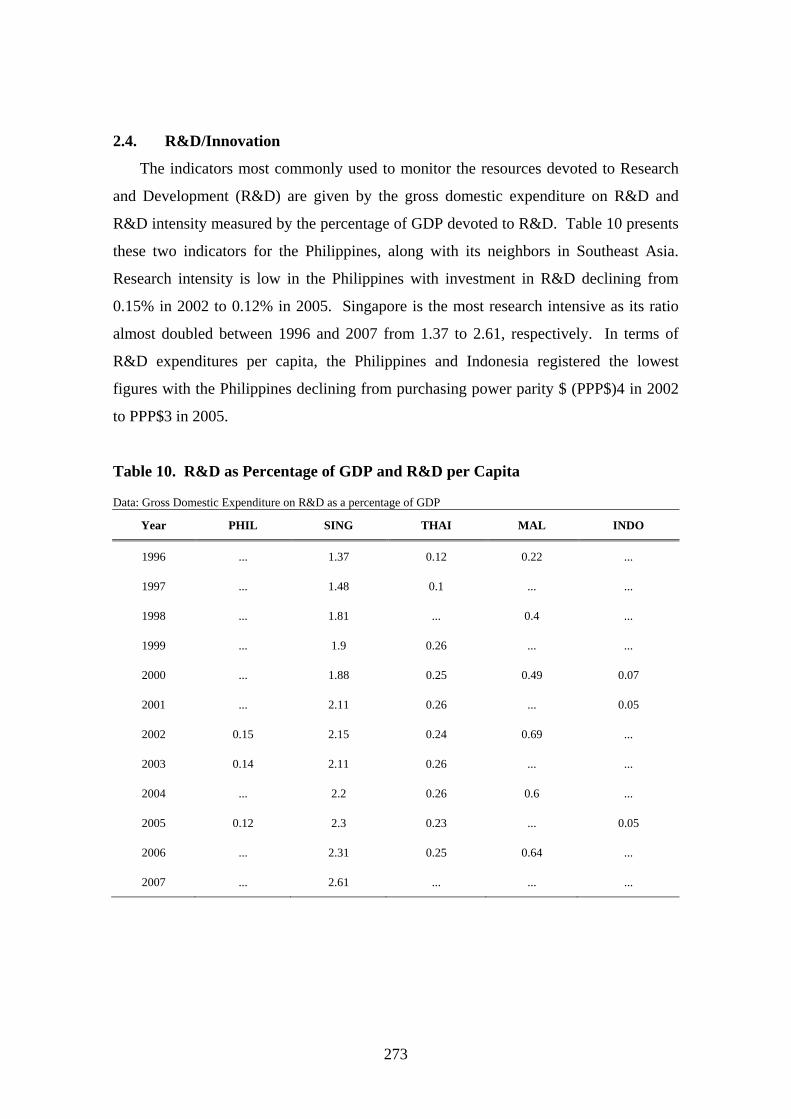
273

2.4. R&D/Innovation

The indicators most commonly used to monitor the resources devoted to Research

and Development (R&D) are given by the gross domestic expenditure on R&D and

R&D intensity measured by the percentage of GDP devoted to R&D. Table 10 presents

these two indicators for the Philippines, along with its neighbors in Southeast Asia.

Research intensity is low in the Philippines with investment in R&D declining from

0.15% in 2002 to 0.12% in 2005. Singapore is the most research intensive as its ratio

almost doubled between 1996 and 2007 from 1.37 to 2.61, respectively. In terms of

R&D expenditures per capita, the Philippines and Indonesia registered the lowest

figures with the Philippines declining from purchasing power parity $ (PPP$)4 in 2002

to PPP$3 in 2005.

Table 10. R&D as Percentage of GDP and R&D per Capita

Data: Gross Domestic Expenditure on R&D as a percentage of GDP

Year PHIL SING THAI MAL INDO

1996 ... 1.37 0.12 0.22 ...

1997 ... 1.48 0.1 ... ...

1998 ... 1.81 ... 0.4 ...

1999 ... 1.9 0.26 ... ...

2000 ... 1.88 0.25 0.49 0.07

2001 ... 2.11 0.26 ... 0.05

2002 0.15 2.15 0.24 0.69 ...

2003 0.14 2.11 0.26 ... ...

2004 ... 2.2 0.26 0.6 ...

2005 0.12 2.3 0.23 ... 0.05

2006 ... 2.31 0.25 0.64 ...

2007 ... 2.61 ... ... ...

274

Table 10 (continued). R&D as Percentage of GDP and R&D per Capita

Data: Gross Domestic Expenditure on R&D per capita (in PPP$)

Year PHIL SING THAI MAL INDO

1996 ... 384 6 18 ...

1997 ... 440 5 ... ...

1998 ... 520 ... 32 ...

1999 ... 578 12 ... ...

2000 ... 632 12 45 2

2001 ... 696 13 ... 1

2002 4 747 13 67 ...

2003 4 764 15 ... ...

2004 ... 882 16 66 ...

2005 3 996 16 ... 2

2006 ... 1104 18 80 ...

2007 ... 1342 ... ... ...

Source: UNESCO Institute for Statistics.

Table 11 presents the number of researchers (measured in full-time equivalent). In

the Philippines, this increased to 6896 in 2005 from 5860 in 2003. Expressed in terms

of researchers per million inhabitants, this went up from 71 in 2003 to 81 in 2005 for the

Philippines. In Singapore, this went up significantly from 2,535 in 1996 to 5,575 in

2005 and to 6,088 in 1007. In Thailand, the ratio increased from 100 in 1996 to 311 in

2005. In Malaysia, this was 503 in 2004 and 205 in Indonesia in 2001.

275

Table 11. Number of Researchers

Data: Researchers (Full Time Equivalent) - Total

YEAR PHILS SING THAI MAL INDO

1996 ... 9108 6038 1894 ...

1997 ... 9704 4409 ... ...

1998 ... 11396 ... 3416 ...

1999 ... 12598 10418 ... ...

2000 ... 16633 ... 6423 44984

2001 ... 16740 17710 ... 42722

2002 ... 18120 ... 7157 ...

2003 5860 20024 18114 ... ...

2004 ... 21359 ... 12670 ...

2005 6896 23789 20506 ... ...

2006 ... 25033 ... 9694 ...

2007 ... 27301 ... ... ...

Data: Researchers per million inhabitants (Full Time Equivalent)

YEAR PHILS SING THAI MAL INDO

1996 ... 2535 100 90 ...

1997 ... 2615 72 ... ...

1998 ... 2977 ... 154 ...

1999 ... 3203 169 ... ...

2000 ... 4139 ... 276 219

2001 ... 4103 281 ... 205

2002 ... 4398 ... 295 ...

2003 71 4820 281 ... ...

2004 ... 5087 ... 503 ...

2005 81 5575 311 ... ...

2006 ... 5736 ... 372 ...

2007 ... 6088 ... ... ...

Source: UNESCO Institute for Statistics.

These figures tend to indicate that the Philippines have been under-investing in

R&D. In a study on R&D gaps in the Philippines, Cororaton (1999) estimated a gap of

0.6% of GDP based on the average ratio in the 1980s. In terms of R&D manpower, the

results showed the need for an additional 197 scientists and engineers per million

276

populations based on the average level in the 1980s. Cororaton also pointed out the

large gap in the country’s institutional structure characterized by a weak national

science and technology system including incentives and protection of intellectual

property rights.

3. Brief Review Of Selected Literature

There are three strands of literature on international trade and growth that are

important in assessing the effects of trade liberalization on innovation: trade and

competition, competition and innovation, and trade and innovation.

Competition and Innovation

The existing theoretical models on competition and innovation point to two

opposing views. Early endogenous growth and Industrial Organization models

suggested that competition appears to be detrimental to innovation and technical

progress. Rents are seen as the major source of innovation for companies wishing to

engage in R&D. Increased competition leads to a decline in innovative activity as more

competition reduces the monopoly rents that reward successful innovators. Hence,

large firms provide a more stable platform for investment in R&D. In contrast, the

opposite view contends that competition may foster innovation as firms need to escape

increased competition from rival firms. Competition will force firms to innovate in

order to survive.

In an effort to reconcile the two views, Aghion et al. (2001) extended the basic

Shumpeterian model by allowing incumbent firms to innovate. Traditional models were

based on the assumption that innovation was done by outsiders or new entrants

competing against incumbents with conventional technology and that the payoff of

innovation was equal to the post-innovation rent (pre-innovation rent was zero). The

Aghion et al. model assumes that innovation incentives depend on the difference

between post-innovation and pre-innovation rents. Firms innovate to reduce production

costs and this is done in a step-by-step manner where a laggard firm must first catch up

277

with the technological leader before becoming a leader. Greater competition may foster

innovation and growth as it may reduce a firm’s pre-innovation rents by more than it

reduces post-innovation rents. Competition may increase the incremental profits from

innovation and encourage R&D investments aimed at escaping competition.

Competition is particularly intense in “neck-and-neck” industries, where competition is

so close that it is hardly possible to determine which firm is leader, and the “escape

competition” effect is strongest in these industries. On the other hand, in less neck-and-

neck or unleveled industries, more competition may reduce innovation as the reward for

laggard firms catching up with the technological leader may fall; this is the

Schumpeterian effect.

The model predicts an inverted-U shaped relationship between competition and

innovation. At low levels of competition, the “escape competition” effect dominates

while at higher levels of competition, the “Schumpeterian effect” dominates. To test the

model, Aghion et al. (2002) used a panel dataset of UK firms. The results confirmed

the presence of a strong inverted U relationship and the gradient of the curve tends to be

steeper for firms that are in more neck-and-neck industries. Looking at entry and

innovation, Aghion and Burgess (2003) showed that competition can affect innovation

depending on the firm’s level of efficiency. In particular, firms close to the efficiency

frontier are expected to survive and deter entry by innovating. An increased entry threat

leads to greater innovation aimed at escaping that threat. In contrast, firms that are far

below the frontier are in a weaker position to fight external entry. An increased entry

threat reduces the payoff from innovating, since the innovation’s expected life horizon

has become shorter. Competition thus provides incentives for more efficient firms to

innovate and a disincentive for less efficient ones. In a related model, Aghion et al.

(2005) predict that firms located in more pro-business environments are more likely to

respond to competition by innovating.

Empirical studies that investigated the relationship between competition and

innovation showed mixed results. The Schumpeterian argument predicts a negative

relationship. Earlier studies that used market concentration as proxy for competition

showed a positive relationship between industry concentration and R&D intensity

(implying a negative relationship). However, more recent studies showed that this

disappears when inter-industry differences such as industry characteristics and

278

technological opportunities are taken into account (Gilbert, 2006). Geroski (1990) did

not find support for the Schumpeterian assertion that monopoly power stimulates

innovation. More recent empirical studies on the relationship between competition and

innovation pointed to a positive relationship. Empirical work by Geroski (1995),

Nickell (1996), and Blundell et al. (1999) found a positive correlation between

competition and innovation. Creusen et al. (2006) also found a positive relationship

between competition and innovation but no evidence for the existence of an inverted –

U.

Hopman and Rojas-Romagosa (2010) analyzed the relationship between changes in

competition levels and innovation efforts. Using OECD panel data, the authors found a

monotonic relationship between the variables, but did not find an inverted-U

relationship as in the influential Aghion et al. (2001) paper. Gorodnichenko et al.

(2009) tested predictions about the impact of competition and linkages with foreign

firms on domestic firms’ innovative efforts, using data on firms in 27 transition

economies. Their findings showed that competition has a negative effect on innovation,

especially for firms that are far from the efficiency frontier. Firms that have market

power tend to innovate more, but greater pressure from foreign competition also

stimulates innovation. The paper did not find support for an inverted U effect of

competition on innovation. Carlin, Schaeffer and Seabright (2004) also tested the

inverted U hypothesis using data on transition economies. The results showed that

innovation is higher in monopolistic industries.

In the Philippines, similar studies linking competition and innovation have not yet

been done. Research work on innovation focused on the estimation of the R&D gap

(Cororaton, 1999) as well as analysis of the state of science and technology and R&D in

the country along with recommendations on how to improve the innovation system and

how to catch up (Cororaton, 2002; Patalinghug, 1999 and 2003; and Macapanpan,

1999). These studies show that the government’s science and technology (S&T) policy

lacks focus and does not provide clear direction for technology innovation. As such, it

has failed to encourage private sector participation despite the R&D incentives granted.

Institutional mechanisms are weak with lack of coordination of planning and budgeting

activities. Major recommendations include improvements in R&D investment,

279

manpower, the incentive system, institutional arrangements and S&T coordination

mechanisms.

Trade and Competition

Since the early 1980s, the new trade theory has shown that aside from the gains

from trade due to specialization based on comparative advantage, trade liberalization

can lead to additional gains by reducing the “deadweight losses” created by the ability

of domestic firms to exercise market power. An open trade regime is a powerful

instrument for disciplining the firms that have market power. Competition from imports

constrains the ability of domestic producers to engage in anti-competitive activities

which would otherwise reduce welfare (Cadot, Grether, & de Melo, 2000). This is

known in the Industrial Organization literature as the “imports-as-competitive

discipline” hypothesis. When confronted with intensified competition, domestic

industries which may have accumulated oligopoly profits in heavily protected markets,

are forced to behave more competitively.

Most of the empirical work on the imports-as-competitive discipline hypothesis

focus on profitability regressions, which regress a measure of profitability such as price

cost margin on import penetration (the ratio of imports to domestic consumption), as a

proxy for trade policy and intensity of import competition and other factors affecting

industry profitability. Since marginal costs are not observable, mark-ups are only

inferred indirectly from price cost margins. Other proxies used for trade policy include

effective protection rates, tariff rates, or import license coverage ratios.

In general, the empirical evidence provides strong support for the imports-as-

competitive discipline hypothesis. Based on industry-level cross-section data,

Schmalensee (1989) indicated that the ratio of imports to domestic consumption tends to

be negatively correlated with the profitability of domestic sellers, especially when

domestic concentration is high. Pugel (1980) also found that import penetration has a

stronger negative relationship with domestic profitability when conventional measures

of entry barriers are high.

Reviewing the literature on the impact of trade liberalization on price cost margins,

Erdem and Tybout (2003) and Tybout (2001) concluded that based on numerous

empirical studies of firm- and plant-level liberalization episodes, mark-ups decline with

280

import competition and this empirical evidence provide robust confirmation for the

import discipline hypothesis. Among import-competing firms, trade liberalization

squeezes price cost margins, inducing some intra-plant efficiency gains as well as

additional efficiency gains due to the closure of weak plants. The authors added that the

effect was particularly marked among large plants. As Roberts and Tybout (1996)

wrote in an earlier paper, in every country studied, relatively high industry-wide

exposure to foreign competition is associated with lower margins and the effect is

concentrated in larger plants.

Using panel data sets on firms, Harrison (1994) examined the results for Cote

d’Ivoire and Krishna and Mitra (1998) for India. Harrison found that mark-ups were

negatively related to import competition in Cote d’Ivoire. In India, Krishna and Mitra

also showed that mark ups fell during the trade reform period. Earlier studies by De

Melo and Urata (1986) and Tybout (1996) for Chile and Grether (1996) for Mexico

showed the same finding. Erdem and Tybout (2003) cautioned that care must be

exercised in interpreting the results. The authors noted that the studies only describe the

short-run effects of trade liberalization. Reforms in trade regimes trigger a dynamic

adjustment process that may take a long time to play out (plausibly lasting more than a

decade).

Other studies showing further evidence that trade liberalization has a pro-

competitive effect include those carried out by Levinsohn (1993) for Turkey; Warzynski

(2002) and J. Konings, Vanseele, and Warzynski (2002) for Romania and Bulgaria; as

well as Goldar and Agarwal (2004), Kambhampati and Parikh (2003), and Srivastava et

al. (2001) for India. These country studies provide support to the import discipline

hypothesis that trade liberalization can lead to substantial reductions in price cost

margins at least in those industries that are imperfectly competitive. For the

Philippines, Aldaba (2007) confirmed the same finding that price cost margins fall with

import competition, and that trade liberalization has a disciplining effect on firms’

pricing behavior.

With the availability of micro data, the recent literature on trade liberalization and

productivity has increased substantially. This body of literature shows that industries

facing the greatest tariff reduction and import competition have faster productivity

growth than relatively protected industries. This is due to resource allocation arising

281

from the exit of inefficient plants and productivity improvements within existing plants.

Empirical studies showing these results were pioneered by Pavcnik (2002) for Chile;

Topalova (2003) for India; Muendler (2002) and Amite and Konings (2007) for

Indonesia, Schor (2003) for Brazil and Fernandes (2007) for Columbia. For the

Philippines, Aldaba (2010) also provided some evidence that trade liberalization leads

to productivity increases. Trade liberalization drives the process of restructuring and

reshuffling of resources within and across sectors of the economy such that unprofitable

activities contract while profitable ones expand. Trade liberalization allows more

productive firms to expand while less efficient firms either exit or shrink. With the exit

of inefficient firms, resources (labor and capital) will be freed and will move to other

industries where they can be used more productively.

Trade and Innovation

Recent literature on trade and growth shows that international trade affects firms’

innovative activities through increased competition. As Licandro (2010) noted,

increasing evidence supports the claim that international trade enhances innovation and

productivity growth through an increase in competition.

In an earlier work based on Schumpeterian growth theory and using firm panel

datasets for India and the UK, Aghion and Burgess (2003) found that reducing barriers

to entry to foreign products and firms has a more positive effect on economic

performance for firms and industries that are initially closer to the technological

frontier. Incumbent firms that are sufficiently close to the technological frontier can

survive and deter entry by innovating. On the other hand, firms that are far below the

frontier are in a weaker position to fight external entry since this will reduce their

expected payoff from innovating. Thus liberalization encourages innovation in

industries that are close to the frontier and discourages innovation in industries that are

far from it. Productivity, outputs, and profits should be higher in the industries and

firms that are initially more advanced. The authors suggested that for countries to

benefit from liberalization, policies that allow firms to upgrade their technological

capabilities or which allow workers to move from low to high productivity sectors are

important.

282

Griffith, Harrison and Simpson (2006) assessed the impact of product market

reforms under the European Union’s (EU)’s Single Market Programme (SMP) on

innovation activity using an unbalanced panel of nine countries and 12 2-digit

manufacturing industries covering the period 1987-2000. Their results suggest that the

SMP’s product market reforms led to an increase in product market competition which

was measured by a reduction in average profitability. Moreover, increased competition

led to an increase in R&D intensity in manufacturing industries. Increased R&D

intensity translated into faster total factor productivity (TFP) growth. The authors

indicated that reforms that put pressure on profitability are likely to lead to increased

innovation.

Fernandes (2009) examined the effects of increased import competition to product

quality upgrading using Chilean manufacturing plant data. The results showed a

positive and significant effect from import competition on product level product quality

upgrading. The author suggested that increased exposure to import competition,

including from China and India, may be beneficial because it encourages producers to

focus on offering upgraded and differentiated products, rather than “mundane” labor

intensive, ones.

Bloom, Draca, and Van Reenen (2010) examined the impact of Chinese import

competition on patenting, IT, R&D and TFP in 12 EU countries using a panel dataset

for the period 1996-2007. The key results are: first, Chinese import competition

increases innovation and TFP within surviving firms. Firms facing higher levels of

import competition from China create more patents, spend more on R&D, raise their IT

intensity and TFP. Secondly, Chinese import competition reduces employment and

survival probabilities in low-tech firms, and these firms’ TFP declines and they exit

much more rapidly than high-tech firms in response to Chinese competition. The

authors noted that the results suggest that increased import competition from China has

caused a significant technological upgrading in European firms through faster diffusion

and innovation. The policy implication is that reducing import barriers against low

wage countries like China can bring about welfare gains through technical change.

283

4. Description Of Methodology And Data

4.1. Overall Framework

The foregoing review highlights three important effects of trade liberalization: trade

reforms increase competition, trade reforms have positive effects on innovation, and

trade reforms lead to the selection of the most productive firms. Trade liberalization

thus has pro-competitive effects and as Bhagwati (1968) wrote, it is seen as a powerful

and administratively simple way to enhance competition Krugman and Helpman (1989)

further noted that international trade increases competition. With trade liberalization,

imports can discipline the market by forcing domestic firms to lower their prices and

behave competitively. Based on a comprehensive review of empirical studies of firm-

and plant-level liberalization episodes in various countries, Erdem and Tybout (2003)

concluded that mark-ups decline with import competition.

Through the competition channel, trade liberalization also has innovation effects.

Newer studies by Fernandes and Bloom, Draca and Van Reenenhave shown some

evidence of the positive impact of trade liberalization on innovation. Economic profits

or rents can serve as rewards for entrepreneurship and encourage innovation. An

increase in competition may increase incentives for incumbent firms to adopt more or to

innovate in order to prevent an erosion of their market position. Note, however, that

increased competition may also reduce the incentive or reward for innovation or entry

and may discourage these activities.

Through the competition channel, trade liberalization also leads to selection effects.

As trade liberalization squeezes price cost margins, some intra-plant efficiency gains are

made, and additional efficiency gains are induced due to the closure of weak plants. In

the presence of within-industry firm heterogeneity, trade liberalization may lead to

improved productivity through the exit of inefficient firms and the reshuffling of

resources and outputs from less to more efficient firms. Melitz (2002) points out that

trade opening may induce a market share reallocation towards more efficient firms and

generate an aggregate productivity gain, without any change at the firm level5. As

                                                        5 In Melitz (2003), the channel through which selection happens is the labor market; trade liberalization increases labor demand, these bids up wages and the cost of production forcing least productive firms to exit the market.

284

Pavcnik, Topalova, and Tybout showed; trade liberalization induces the least productive

firms to exit the market and the most productive non-exporters to become exporters.

Impulliti and Licandro (2009, 2010)6 introduced a framework that attempts to link

together these three effects of trade liberalization. Basically, trade affects both firm

selection and innovation through the competition channel. Trade liberalization leads to

an increase in the number of firms in the domestic market raising product market

competition and lowering the markup rate. The selection effect of trade operates

through endogenous markups resulting from oligopolistic competition7 among firms.

The reduction in the markup rate (or increase in competition) due to trade liberalization

reduces profits, raises the productivity threshold above which firms can profitably

produce and forces the less productive firms out of the market. Resources are

reallocated from exiting firms to the higher productivity surviving firms which innovate

at a faster pace.

Given the relationship between trade liberalization and innovation operating

through the competition channel, the impact of trade liberalization on innovation is

examined through a two-stage approach where competition is endogenous. The same

framework was used by Griffith, Harrison, and Simpson (2006) to address the

endogeneity of competition in analyzing the relationship between product market

reform and innovation in the EU. The following basic econometric model is tested:

Competition function

 Competition  f Trade  , Z equation (1)

Innovation function

 

Innovation   Competition  , Z equation (2)

Where i indexes firms, j industries and t years. Equation (1) describes the relationship

between trade reforms and competition while equation (2) characterizes the relationship

between innovation and competition and links trade reforms with innovation through

                                                        6 Both are preliminary and incomplete draft versions. 7 In Melitz (2003), the model assumes monopolistic competition.

285

competition. Z is a vector of control variables that may affect the firm’s innovation

efforts.

Following Aghion et al. (2002), the price cost margin is used as an indicator of

product market competition, while research and development expenditures are used as a

proxy for innovation. The authors noted that the price cost margin has several

advantages over other indicators such as market shares, the Herfindahl index, or the

concentration index. These measures require a definition of both the geographic and

product boundaries of the market in which the firm operates. This becomes important

particularly for firms that operate in international markets, so that traditional market

concentration measures could be extremely misleading.

The specific competition and innovation functions are described by equations (3)

and (4) below:

equation (3)

equation (4)

where PCM is price cost margin, Tariff is a trade reform indicator, TGap or technology

gap is the distance to the technological frontier and is a measure of efficiency, RD is

research and development expenditures, Age and Size are firm characteristics measured

by firm age and total number of workers, respectively; Time and Ind are time and

industry dummies, and and are error terms. Apart from output tariff, effective

protection rate (EPR) will also be used as a trade reform indicator. EPRs represent rates

of protection of value added and measure the net protection received by domestic

producers from the protection of their outputs and the penalty from the protection of

their inputs.

To control for the effects of the selection process on competition and innovation,

net entry is also incorporated in the model:

PCM ijt 0Tariffjt 1TGap ijt 2Age ijt 3Size ijt 4 Time 5Ind ijt

RD ijt 0PCM ijt 1TGap ijt 2Age ijt 3Size ijt 4 Time 5Ind ijt

286

equation (3a)

equation (4a)

A positive relationship is expected between competition (as measured by PCM) and

trade liberalization (with Tariff and EPR as indicators). As tariffs or EPRs are lowered,

price cost margin or profitability is reduced, which indicates increased competition.

This is the main channel through which trade liberalization affects innovation. Hence,

the trade indicators (Tariff and EPR) do not directly enter equation (4).

A negative relationship is expected between PCM (measure of competition) and RD

(measure of innovation). As price cost margin or profitability is reduced due to trade

reforms, competition increases raising the productivity threshold above which firms can

profitably produce. This forces less productive firms out of the market. Resources are

reallocated from exiting firms to the higher productivity surviving firms which innovate

at a faster pace.

The price cost margin (PCM) or Lerner index is an indicator of the level of

competition or degree of monopoly power of firms in industries. It is often used as an

indicator of the strength of competition in the market. In theory, it is defined as price

minus marginal cost over price and reflects the degree of monopoly power measured by

the mark-up pricing above marginal costs (see Appendix 1). It should be noted that

high PCMs are not necessarily an indication of bad market performance or that a firm is

less competitive. While a high PCM implies market power, it could also indicate high

firm efficiency. If these high mark-ups or margins are the result of internal efficiency

improving measures or represent gains from product innovation or techniques that a

firm employs, then the firm is still considered competitive.

The empirical measurement of PCM is difficult since marginal costs are not directly

observable and are quite hard to estimate. Indirect measures have been developed based

on accounting data, with average variable costs acting as proxy for marginal costs.

Critiques noted that measured in this manner, PCM omits capital costs and becomes a

poor indicator of excess profits.

PCMijt

0Tariff

jt

1TGap

ijt

2Age

ijt

3Size

ijt

4NetEntry

jt

5Time

6Ind

ijt

RDijt

0PCM

ijt

1TGap

ijt

2Age

ijt

3Size

ijt

4NetEntry

ijt

5Time

6Ind

ijt

287

Aghion et al. (ibid) used operating profits net of depreciation and provisions less

the financial cost of capital. This is given by the following:

B  Operating profits Financial cost of capital

Sales

where Financial cost of capital is defined as     . They assumed

the cost of capital to be 0.085 for all firms and time periods while capital stock is

measured using the perpetual inventory method. Measured this way, it is more like the

ratio of price less average cost to price. Note that in 1988, Hall developed an alternative

way to measure mark-ups from the production function of firms. Using the properties

of the Solow residual under perfect competition, Hall derived an empirical specification

that allows the retrieval of industry wide mark-ups (measured by price/marginal costs).

Comparing the econometrically estimated PCMs with calculated accounting margins,

Siotis (2003) found that overall, the accounting margins approach yields reasonable and

precise estimates indicating that accounting based PCM measures may not be as flawed

as previously thought, at least when the sample size is large both within the sample and

over time.

In this paper, the PCM is defined as:

B   T   C T   F      

T  

where the implicit price index for gross domestic capital formation is used as a price

index of investment goods while the 180-day Treasury Bill interest rate less inflation is

used as measure of real interest rate.

Aghion et al. (ibid) measure the technology gap between firms within an industry as

the proportional distance a firm is from the technological frontier. In this paper, this is

given by the difference between the log total factor productivity (TFP) of the most

productive firm in a given industry and log TFP of each firm in the industry.

Total cos ts Raw materials Fuel Electricity DepreciationOther cos ts

Financialcos t of capital [ Index of investment goods * Re al int erest rate]* Book value of assets

equation (5)

equation (6)

288

Domestic firms are differentiated depending on the trade orientation of their

industry sector. Firms in a traded sector are more exposed to foreign competition than

firms in a non-traded sector. Based on the sector’s import penetration ratio, and export

intensity ratio calculated from the year 2000 Input-Output Table, each industry sector is

classified into traded or non-traded. A sector is classified as non-traded if export and

import ratios are zero or less than 1%. This includes manufacturing sub-sectors such as

slaughtering and meat packing, ice cream, mineral water, and custom tailoring and

dressmaking.

A traded sector is categorized into three: purely importable, purely exportable, or

mixed. A purely exportable sector is characterized by zero or minimal imports and

substantial exports or an export ratio of at least 10%. Examples are tobacco leaf flue-

curing, articles made of native materials, wood carvings, fish drying, knitted hosiery,

crude coconut oil, rattan furniture, and jewelry. A purely importable sector is

characterized by minimal exports and significant imports or an import ratio of at least

10%. Examples are meat and meat products, coffee roasting and processing, butter and

cheese, animal feeds, starch and starch products and manufacture and assembly of

motor vehicles. A mixed sector has substantial imports and exports such as motor

vehicle parts and components, semi-conductor, parts and supplies for radio, TV,

communication, appliances and house wares, garments, carpets and rugs, furniture,

along with sugar, glass, chemicals, cigarette, soap and detergents, iron and steel and

drugs and medicines. Notice that a lot of the products under both the mixed and purely

importable sectors are also among the products with tariff peaks8. Moreover, aside from

tariff protection, certain products under these sectors also received additional protection

through safeguard measures that are imposed on importations of cement, glass,

chemicals, and ceramic tiles.

                                                        8 Tariff peaks refer to tariffs that are greater than three times the mean tariff. The sectors with tariff peaks were sugarcane, sugar milling and refining, palay, corn, rice and corn milling, vegetables such as onions, garlic, and cabbage, roots and tubers, hogs, cattle and other livestock, chicken, other poultry and poultry products, slaughtering and meat packing, coffee roasting and processing, meat and meat processing, canning and preserving fruits and vegetables, manufacture of starch and starch products, manufacture of bakery products excluding noodles, manufacture of animal feeds, miscellaneous food products, manufacture of drugs and medicines, manufacture of chemical products, and manufacture and assembly of motor vehicles.

289

4.2. Data

The paper uses the firm level panel data created in the first Micro Data Project of

the Economic Research Institute for ASEAN and East Asia (ERIA).9 The dataset

consists of firm level information on revenues, employment, compensation, physical

capital, R&D expenditures, and production costs from the Annual Survey and Census of

Establishments of the National Statistics Office (NSO). The firm-level panel dataset

built covered the period 1996 to 2006, with three missing years (1999, 2001, and 2004).

The years 2000 and 2006 are both census years while the remaining six years are

surveys.

The panel dataset is unbalanced and covers all firms with two or more overlapping

years during the period 1996-2006. Firms with missing zero or negative values for the

variables listed above as well as firms with duplicates were dropped. Firms with

missing research and development expenditures and those with less than 10 workers

were also excluded. Firm exit is indicated by firms that are no longer included in the

2006 census as well as those whose 2-digit PSIC codes have changed. Firm entry is

defined based on the firm’s year of establishment or year when it started operating. Net

entry by PSIC code is calculated as firm entry less exit. Firm age is calculated based on

the firm’s year of establishment or year when it started operating. The panel dataset is

unbalanced with a total of 8,296 observations. Table 12 presents a summary of the data

along with the calculated price cost margins and financial cost of capital.

                                                        9 The National Statistics Office provided excellent assistance in building the panel dataset. 

290

Table 12. Summary Statistics

Variable Obs Mean Std. Dev. Min Max

Total revenue (in million pesos) 8296 736 5200 0.065 233000

Compensation (in million pesos) 8296 43 141 0 2640

Total costs (in million pesos) 8296 594 4510 0.026 203000

Book value of fixed assets (in million pesos) 8296 180 1000 0 47600

Capital cost 8296 0.07 0.059 0.03 0.219

Financial cost of capital (in million pesos) 8296 15 102 0 5750

Price cost margin 8296 0.053 0.259 -6.086 0.96

R&D expenditure share (as % of value added) 8296 0.005 0.068 0 5.373

Age of firm (in years) 8263 17 14 0 100

Total number of workers 8296 264 703 10 14647

TFP Gap 8296 0.371 0.146 0 1.054

Tariff (in percent) 8296 9.087 6.309 1.073 60

Net entry 8296 -3 6.9 -52 6

Tariff rates by manufacturing sub-sector were obtained from the Philippine Tariff

Commission. The tariff rates are originally coded based on Harmonized System (HS)

codes. These were converted into the Philippine System of Industry Classification

(PSIC) code to be consistent with the firm level data. Effective protection rates (EPRs

were sourced from studies by Manasan and Pineda (1999) for the 1990s and Aldaba

(2005) for EPRs in the more recent period.

The TFP Gap indicator was calculated based on the total factor productivity (TFP)

estimates obtained from an earlier ERIA study by Aldaba (2010). TFP is defined as the

residual of a Cobb-Douglas production function and is estimated using the methodology

of Levinsohn and Petrin (2001). In estimating the production function, data on value

added (output less cost of materials and energy) and two factors of production, labor

and capital, were used. Fuel and electricity data were employed as proxy for

productivity shocks.10 A production function was estimated for 11 industry-sectors.

The estimates of firm i’s TFP is obtained by subtracting firm i’s predicted y (or log of

output) from its actual y at time t. To make the estimated TFP comparable across

                                                        10 To address the simultaneity problem in input choice when estimating the production function by ordinary least squares (OLS), a semi-parametric estimator with an instrument to control for unobserved productivity shocks is applied. For this instrument, Olley and Pakes (1996) use investment while Levinsohn and Petrin (2002) suggest the use of intermediate inputs.

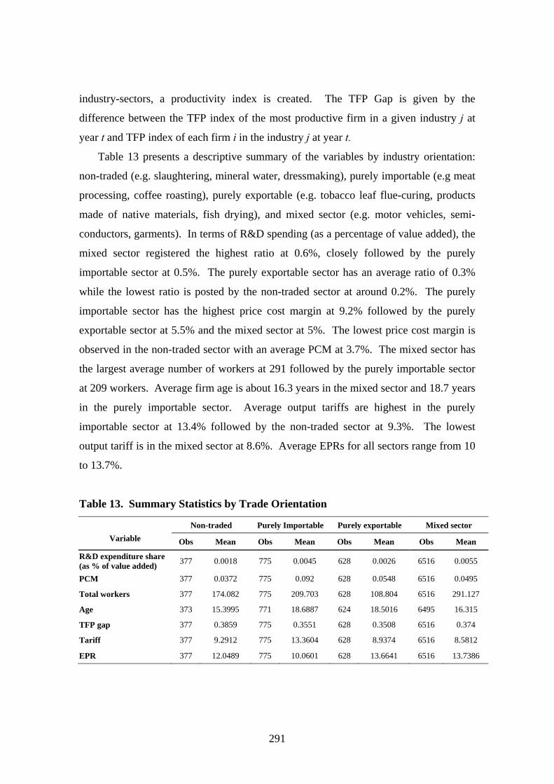
291

industry-sectors, a productivity index is created. The TFP Gap is given by the

difference between the TFP index of the most productive firm in a given industry j at

year t and TFP index of each firm i in the industry j at year t.

Table 13 presents a descriptive summary of the variables by industry orientation:

non-traded (e.g. slaughtering, mineral water, dressmaking), purely importable (e.g meat

processing, coffee roasting), purely exportable (e.g. tobacco leaf flue-curing, products

made of native materials, fish drying), and mixed sector (e.g. motor vehicles, semi-

conductors, garments). In terms of R&D spending (as a percentage of value added), the

mixed sector registered the highest ratio at 0.6%, closely followed by the purely

importable sector at 0.5%. The purely exportable sector has an average ratio of 0.3%

while the lowest ratio is posted by the non-traded sector at around 0.2%. The purely

importable sector has the highest price cost margin at 9.2% followed by the purely

exportable sector at 5.5% and the mixed sector at 5%. The lowest price cost margin is

observed in the non-traded sector with an average PCM at 3.7%. The mixed sector has

the largest average number of workers at 291 followed by the purely importable sector

at 209 workers. Average firm age is about 16.3 years in the mixed sector and 18.7 years

in the purely importable sector. Average output tariffs are highest in the purely

importable sector at 13.4% followed by the non-traded sector at 9.3%. The lowest

output tariff is in the mixed sector at 8.6%. Average EPRs for all sectors range from 10

to 13.7%.

Table 13. Summary Statistics by Trade Orientation

Variable

Non-traded Purely Importable Purely exportable Mixed sector

Obs Mean Obs Mean Obs Mean Obs Mean

R&D expenditure share (as % of value added)

377 0.0018 775 0.0045 628 0.0026 6516 0.0055

PCM 377 0.0372 775 0.092 628 0.0548 6516 0.0495

Total workers 377 174.082 775 209.703 628 108.804 6516 291.127

Age 373 15.3995 771 18.6887 624 18.5016 6495 16.315

TFP gap 377 0.3859 775 0.3551 628 0.3508 6516 0.374

Tariff 377 9.2912 775 13.3604 628 8.9374 6516 8.5812

EPR 377 12.0489 775 10.0601 628 13.6641 6516 13.7386

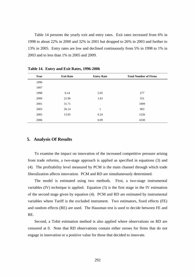
292

Table 14 presents the yearly exit and entry rates. Exit rates increased from 6% in

1998 to about 22% in 2000 and 32% in 2001 but dropped to 26% in 2003 and further to

13% in 2005. Entry rates are low and declined continuously from 5% in 1998 to 1% in

2003 and to less than 1% in 2005 and 2009.

Table 14. Entry and Exit Rates, 1996-2006

Year Exit Rate Entry Rate Total Number of Firms

1996

1997

1998 6.14 5.05 277

2000 21.96 1.63 551

2001 31.71 1009

2003 26.14 1 903

2005 13.05 0.24 1226

2006 0.09 4330

5. Analysis Of Results

To examine the impact on innovation of the increased competitive pressure arising

from trade reforms, a two-stage approach is applied as specified in equations (3) and

(4). The profitability level measured by PCM is the main channel through which trade

liberalization affects innovation. PCM and RD are simultaneously determined.

The model is estimated using two methods. First, a two-stage instrumental

variables (IV) technique is applied. Equation (3) is the first stage in the IV estimation

of the second stage given by equation (4). PCM and RD are estimated by instrumental

variables where Tariff is the excluded instrument. Two estimators, fixed effects (FE)

and random effects (RE) are used. The Hausman test is used to decide between FE and

RE.

Second, a Tobit estimation method is also applied where observations on RD are

censored at 0. Note that RD observations contain either zeroes for firms that do not

engage in innovation or a positive value for those that decided to innovate.

293

5.1. All Manufacturing: No Entry and Exit Indicators

Table 15.1 presents the results of the first stage of the IV estimation which

evaluates the degree of correlation between trade reforms, as measured by Tariff, and

the endogenous regressor, PCM, which is our measure of profitability. The first stage

regression results suggest that the excluded instrument Tariff is highly correlated with

PCM based on both the FE and RE methods. The coefficient on Tariff is positive and

highly significant indicating that trade reforms have a strong positive impact on the

level of profitability. The results also show a negative association between TFP Gap

and profitability. The coefficient on TFP Gap is negative and highly significant in both

FE and RE methods. This indicates that firms that are farther from a technological

frontier (less productive firms) have lower profitability than efficient firms which tend

to have higher profitability.

Table 15.1. First Stage IV Results: FE and RE

ALL MANUFACTURING

PCM Tariff EPR

(1) FE (2) RE (1) FE (2) RE

Age 0.00031 -0.000458* -0.0039674 -0.0008581*

0.0026855 0.0002743 0.0022206 0.000539

Total workers -0.00001 -0.000028*** -8.15E-06* -0.0000241***

0.0000128 0.0000054 0.0000128 6.94E-06

TFP Gap -2.54176*** -1.483633*** -2.557112 -2.08648***

0.1052527 0.04587 0.1052544 0.0568845

Trade 0.0069049*** 0.002489*** 0.0006741 0.0004895

0.0022272 0.0007028 0.0004289 0.0002319

Constant 1.096718*** 0.5535773*** 1.254195

0.1022577 0.0254748 0.0889347

Year Dummies Y Y Y Y

Industry Dummies Y Y Y Y

F-Statistic 1.65 1.65

Prob>F 0 0

Observations 8263 8263 8263 8263

R-squared 0.0672

Hausman Test

Chi2 45.22 8.27

Prob>chi2 0.0001 0.9605

Note: * 10% level of significance, **5% level of significance, ***1% level of significance.

294

Using EPR as a trade indicator, the random effects method shows that the

coefficient on EPR is positive but not significant. The coefficient on total workers is

negative and highly significant. The coefficient on TFP Gap is also negative and highly

significant while the coefficient on age is negative and significantly different from zero.

Table 15.2 presents the results of the second stage IV estimation, which looks at the

relationship between profitability and innovation where RD is the dependent variable.

The FE results based on Tariff as trade indicator show a significant negative

relationship between PCM and RD which indicates that reduced profitability

(suggesting high competition) due to trade reform is associated with increased RD. The

RE results show the same negative relationship between PCM and RD, but not at a

significant level. The coefficient on TFP Gap is negative in both FE and RE methods

but is insignificant.

Table 15.2. Second Stage IV Results: FE and RE

RD Tariff EPR

(1) FE (2) RE (1) FE (2) RE

PCM -0.114983* -0.095598 -0.074743 -0.111575

-0.0704618 -0.0776039 -0.129896 -0.111468

Age -0.00044 0.0001051 -0.000256 0.0000963

-0.0005744 -0.000084 -0.000737 -0.000158

Total workers -0.00000538* -2.25E-06 -5.06E-06* -4.56E-06

-0.00000285 -0.00000265 -2.81E-06 -3.16E-06

TFP Gap -0.11871 -0.0520831 -0.015795 -0.096095

-0.1816651 -0.1146816 -0.332906 -0.232484

Constant 0.09242 0.027075 0.0419677 0.0494711

-0.0904484 -0.0444074 -0.163868 -0.095103

Year Dummies Y Y Y Y

Industry Dummies Y Y Y Y

F-Statistic 3.13 3.57

Prob>F 0 0

Observations 8263 8263 8263 8263

R-squared 0.0044

Hausman Test

Chi2 45.22 8.27

Prob>chi2 0.0001 0.9605

Note: * 10% level of significance, **5% level of significance, ***1% level of significance.

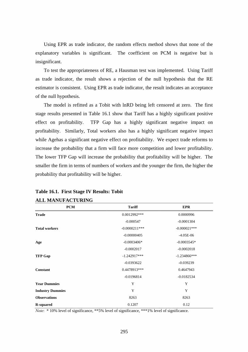
295

Using EPR as trade indicator, the random effects method shows that none of the

explanatory variables is significant. The coefficient on PCM is negative but is

insignificant.

To test the appropriateness of RE, a Hausman test was implemented. Using Tariff

as trade indicator, the result shows a rejection of the null hypothesis that the RE

estimator is consistent. Using EPR as trade indicator, the result indicates an acceptance

of the null hypothesis.

The model is refitted as a Tobit with lnRD being left censored at zero. The first

stage results presented in Table 16.1 show that Tariff has a highly significant positive

effect on profitability. TFP Gap has a highly significant negative impact on

profitability. Similarly, Total workers also has a highly significant negative impact

while Agehas a significant negative effect on profitability. We expect trade reforms to

increase the probability that a firm will face more competition and lower profitability.

The lower TFP Gap will increase the probability that profitability will be higher. The

smaller the firm in terms of numbers of workers and the younger the firm, the higher the

probability that profitability will be higher.

Table 16.1. First Stage IV Results: Tobit

ALL MANUFACTURING PCM Tariff EPR

Trade 0.0012992*** 0.0000996

-0.000547 -0.0001304

Total workers -0.0000211*** -0.000021***

-0.00000405 -4.05E-06

Age -0.0003406* -0.0003545*

-0.0002017 -0.0002018

TFP Gap -1.242917*** -1.234866***

-0.0393622 -0.039239

Constant 0.4478913*** 0.4647943

-0.0196814 -0.0182534

Year Dummies Y Y

Industry Dummies Y Y

Observations 8263 8263

R-squared 0.1207 0.12

Note: * 10% level of significance, **5% level of significance, ***1% level of significance.

296

With EPR as trade indicator, the first stage results show that the coefficient on EPR

is positive but not significant. The coefficient on TFP is negative and highly significant.

The coefficient on total workers is also negative and highly significant. For age, the

coefficient is negative and significant.

The second stage Tobit results are presented in Table 16.2. The results show that

with Tariff as trade indicator, PCM has a significant negative effect on lnRD. The

lower profitability (suggesting higher competition) will increase the probability that a

firm will engage in R&D activities and will increase its R&D intensity. The Tobit

results also show a highly significant negative effect for Total workers and negative

effect for Age. With EPR as trade indicator, none of the explanatory variables is

significant. The coefficient on PCM is negative but insignificant.

Table 16.2. Second Stage IV Results: Tobit

LnRD Tariff EPR

PCM -10.44935* -10.05107

-5.906214 -17.95807

Total workers -0.0005009*** -0.0004926

-0.0001365 -0.0003815

Age -0.0064991* -0.0063593

-0.0035068 -0.0068841

TFP Gap -5.04204 -4.551069

-7.30149 -22.14417

Constant -0.5995352 -0.7849602

-2.761603 -8.364468

Year Dummies Y Y

Industry Dummies Y Y

Observations 8263 8263

R-squared 0.1207 0.12

Note: * 10% level of significance, **5% level of significance, ***1% level of significance.

On the whole, using tariffs as trade indicator, the results tend to confirm that trade

liberalization may stimulate firms to innovate through competition. For EPR, however,

this is not the case. While the correct signs on the coefficient of EPR and PCM are

obtained, these are not significant. Regarding the TFP gap, the expected negative

relationship is found, however, the result is also not statistically significant.

297

5.2. All Manufacturing: With Entry and Exit Indicators

Tables 17.1-18.2 show the results with an additional control variable for exit and

entry measured by net entry. Using IV, the first stage results indicate a strong positive

impact of trade liberalization on competition based on both tariff and EPR as trade

indicators. As tariffs (and EPRs) decline, price cost margin or profitability is reduced

which indicates increased competition. The coefficient on TFP Gap is negative and

highly significant. The coefficient on Net Entry is also negative but insignificant.

Table 17.1. First Stage IV Results: FE and RE

ALL MANUFACTURING

PCM EPR TARIFF

(1) FE (2) RE (1) FE (2) RE

Age -0.0039215* -0.0007018* 0.0003441 -0.0004529*

standard error 0.0022208 0.0004111 0.0026855 0.0002718

Total workers -0.00000818 -0.0000282*** -5.38E-06 -0.0000279***

standard error 0.0000128 0.00000648 0.0000128 5.37E-06

TFP Gap -2.557469*** -1.864594*** -2.54216*** -1.475161***

standard error 0.1052466 0.0532788 0.1052451 0.0456886

Net Entry -0.0007582 -0.000508 -0.0007556 -0.0001445

standard error 0.0006247 0.0004102 0.0006239 0.0004494

Trade Indicator 0.0006674 0.000427** 0.006884*** 0.0024462***

standard error 0.0004289 0.0002165 0.0022271 0.0006985

Constant 1.255121 1.098123***

standard error 0.088931 0.1022564

Year Dummies Y Y Y Y

Industry Dummies Y Y Y Y

Observations 8263 8263 8263 8263

R-squared (overall) 0.0694 0.0669

Hausman Test

Chi2 13.32 52.66

Prob>chi2 0.7145 0.0000

Note: * 10% level of significance, **5% level of significance, ***1% level of significance.

298

Table 17.2. Second Stage IV Results: FE and RE

RD EPR TARIFF

(1) FE (2) RE (1) FE (2) RE

PCM -0.0739931 -0.1189551 -0.1148789* -0.0916575

standard error 0.1310972 0.1272509 0.0706754 0.0784155

Age -0.0002561 0.0000955 -0.0004381 0.0001054

standard error 0.0007356 0.000136 0.000573 0.0000833

Total workers -0.00000505* -0.00000422 -0.00000538* -2.09E-06

standard error 0.00000282 0.00000396 0.00000285 2.65E-06

TFP Gap -0.0138511 -0.1017999 -0.1184321 -0.0459054

standard error 0.3360179 0.2370014 0.1822321 0.1152147

Net Entry 0.0000574 0.0000826 0.0000259 0.0001785

standard error 0.0171815 0.0001225 0.0001468 0.0001243

Constant 0.0409574 0.0471517 0.0922571 0.0306018

standard error 0.1654865 0.092097 0.0907753 0.0469146

Year Dummies Y Y Y Y

Industry Dummies Y Y Y Y

Observations 82633 8263 8263 8263

R-squared (overall) 0.0047 0.0102 0.0044 0.0118

Note: * 10% level of significance, **5% level of significance, ***1% level of significance.

In the second stage, the results based on the fixed effects (FE) method with Tariff as

trade indicator, show some evidence of a positive effect of competition on innovation

brought about by trade liberalization. The coefficient on PCM is negative and

significant at the 10% level. The coefficient on Total workers is negative and

significant. The coefficient on TFP gap is negative but not statistically significant. In

the case of EPR as trade indicator, the random effects (RE) results show that although

the coefficient on PCM is negative, it is not significant. It is important to note that the

EPRs used are based only on output and input tariff rates and do not take into account

the presence of non-tariff barriers, such as import controls and restrictions, which are

more binding than tariffs. Although tariff rates are reduced, importation is still limited

299

due to the presence of these restrictions. This may be one possible explanation of why

in most cases, though EPR has the correct sign, it is not significant.11

Tables 18.1-18.2 present the results of the first and second stages, respectively,

using a Tobit regression. Based on Tariff as trade indicator, trade liberalization has a

positive effect on innovation through competition. The results show a positive

relationship between tariff and PCM and a negative relationship between PCM

(measure of competition) and RD (measure of innovation).

Table 18.1. First Stage TOBIT

ALL MANUFACTURING PCM EPR TARIFF

Trade Indicator 0.0000993 0.0012991***

standard error 0.0001304 0.0005476

Total workers -0.000021*** -0.0000211***

standard error 0.00000405 0.00000405

Age -0.0003541* -0.0003405*

standard error 0.0002018 0.0002018

TFP Gap -1.234975*** -1.242921***

standard error 0.0392628 0.0393829

Net Entry -0.0000404 -0.00000138

standard error 0.0004832 0.0004833

Constant 0.4647379*** 0.4478903***

standard error 0.0182669 0.0196862

Year Dummies Y Y

Industry Dummies Y Y

Observations 8263 8263

Adj R-squared 0.118 0.1186

                                                        11 Import ratios were also calculated as an alternative trade indicator. However, the inconsistencies in using matched aggregated import data at the industry level with the survey and census data prevented us from using them.

300

Table 18.2. Second Stage TOBIT

LnRD EPR TARIFF

PCM -11.70061 -11.17755*

standard error 19.68247 6.144492

Total workers -0.0005295 -0.0005185***

standard error 0.0004182 0.000142

Age -0.0067569 -0.0065736*

standard error 0.0075315 0.0036446

TFP Gap -6.638679 -5.993806

standard error 24.27343 7.596961

Net Entry -0.0188524*** -0.0188251***

standard error 0.0073079 0.0070451

Constant -0.0445921 -0.2880717

standard error 9.166121 2.872541

Year Dummies Y Y

Industry Dummies Y Y

Observations 8263 8263

R-squared

Note: * 10% level of significance, **5% level of significance, ***1% level of significance.

In the first stage, the coefficient on TFP gap is negative and highly significant.

Similarly, the coefficient on Total Workers is negative and highly significant. The

coefficient on Net Entry is negative but is insignificant. In the second stage, the

coefficient on Net Entry is negative and highly significant indicating that higher net exit

will increase the probability that surviving firms will engage in R&D activities. Note

that as tariffs decline, price cost margin or profitability is reduced, competition increases

and less efficient firms are forced out of the market. The coefficient on Age is negative

and significant and similarly, the coefficient on Total Workers is negative and highly

significant. Based on EPR as trade indicator, the evidence that trade liberalization leads

to innovation is relatively weaker. The coefficient on PCM is negative, but not

significant.

5.3. Manufacturing by Trade Orientation: No Entry and Exit Indicators

The model is next tested using the different manufacturing sectors classified based

on their trade orientation: non-traded, purely importable, purely exportable, and mixed

301

sector. Two regressions methods are applied, IV and Tobit. For IV, two estimation

techniques are applied: FE and RE.Two trade indicators are used, output tariffs and

effective protection rates.

Tables 19.1-20.2 summarize the key results for the mixed sectors. Using IV

regression and Tariff as trade indicator, some evidence of a positive effect of trade

liberalization on innovation is found. The coefficient on Tariff is positive and highly

significant while the coefficient on PCM is negative and significant. Using EPR as

trade indicator, the coefficient is positive and highly significant, but for PCM, while the

coefficient is negative it is not significant.

Table 19.1. First Stage IV Results: FE and RE

MIXED SECTOR

PCM EPR TARIFF

(1) FE (2) RE (1) FE (2) RE

Age -0.002196 -0.0007068 0.000307 -0.0006029

-0.0025562 -0.0004806 -0.0032214 -0.0004183

Total workers -9.02E-06 -.0000277*** -9.32E-06 -.0000288***

-0.0000131 -6.69E-06 -0.0000131 -6.37E-06

TFP Gap -2.663347*** -1.983007*** -2.664046*** -1.855282***

-0.1171964 -0.061406 -0.1172395 -0.0592093

Trade Indicator .0024892*** .0017411*** .0075801** .006108***

-0.0009776 -0.000455 -0.0034387 -0.0014744

Constant .9566725*** .8702728***

-0.1404109 -0.1532073

Year Dummies Y Y Y Y

Industry Dummies Y Y Y Y

Observations 6495 6495 6495 6495

R-squared (overall) 0.0723 0.0736

Hausman Test

Chi2 9.67 9.23

Prob>chi2 0.9169 0.9329

302

Table 19.2. Second Stage IV Results: FE and RE

MIXED SECTOR

RD EPR TARIFF

(1) FE (2) RE (1) FE (2) RE

PCM -0.0552967 -0.0906546 -0.1351851 -.1295984*

-0.0833932 -0.0678799 -0.107184 -0.0682428

Age -0.0000902 0.0001219 -0.0004435 0.0001018

-0.0006294 -0.0001337 -0.0007396 -0.0001255

Total workers -4.91e-06* -3.09E-06 -5.67e-06* -3.80E-06

-2.89E-06 -2.58E-06 -3.26E-06 -2.70E-06

TFP Gap 0.0258156 -0.0453125 -0.1875423 -0.1114657

-0.2241031 -0.1348436 -0.2875925 -0.126285

Constant 0.0048743 0.0256419 0.0858808 0.0527683

-0.0895349 -0.0546182 -0.1135132 -0.0512104

Year Dummies Y Y Y Y

Industry Dummies Y Y Y Y

Observations 6495 6495 6495 6495

R-squared (overall) 0.0043 0.0124 0.0045 0.0112

The same results are obtained in the Tobit regression; both EPR and tariff have the

correct positive signs which are highly significant; however, while the coefficient on

PCM is negative as expected, it is not significant. The results also show a highly

significant negative relationship between PCM and TFP gap and a highly significant

negative relationship between number of workers and R&D.

303

Table 20.1. First Stage IV Results: Tobit

MIXED SECTOR PCM (1) TARIFF (2) EPR

Age -.0003994 * -.0003936*

-0.0002435 -0.0002436

Total workers -.0000216*** -.0000219***

-4.33E-06 -4.34E-06

TFP Gap -1.332122*** -1.322314***

-0.0474155 -0.0472372

Trade Indicator .0030229*** .0005372*

-0.001026 -0.0002858

Constant .4655379*** .5039854***

-0.0301794 -0.0258772

Year Dummies Y Y

Industry Dummies Y Y

Observations 6495 6495

Adj R-squared 0.1189 0.1182

Table 20.2. Second Stage IV Results: Tobit

LnRD (1) TARIFF (2) EPR

PCM -5.733137 -8.414397

-3.639965 -6.594807

Total workers -.0003721*** -.000431***

-0.0000925 (.0001546)*

Age -.0060584** -0.0070863

-0.0029606 -0.003938

TFP Gap 0.9419193 -2.583998

-4.813166 -8.691929

Constant -5.503807*** -4.12588

-1.890225 -3.403656

Year Dummies Y Y

Industry Dummies Y Y

Observations 6495 6495

304

For the other remaining sectors- non-traded, purely importable, and purely

exportable- the evidence that trade liberalization affects innovation through competition

seems to be weak. The general results show that although the coefficient on the trade

indicator (EPR or Tariff) is correct, it is not significant. Similarly, the coefficient on

PCM has the correct sign but is also not significantly different from zero.

5.4. Manufacturing by Trade Orientation: With Entry and Exit Indicators

The next set of results use the same basic model with a control variable for the

selection process measured by Net Entry. Tables 21.1 to 22.2 present the results for the

mixed sector. With Net Entry as an additional control variable, the results based on

Tariff as trade indicator show some evidence of a positive effect of competition on

innovation brought about by trade liberalization.

Using IV regression with Tariff as trade indicator, the REfirst stage results show

that Tariff and PCM have a positive relationship that is highly significant. TFP and

PCM have a highly significant negative relationship indicating that less efficient firms

have lower profitability. The coefficient on Total Workers is negative and highly

significant. The second stage results show that PCM and R&D have a significant

negative relationship.

305

Table 21.1. First Stage IV Results: FE and RE

MIXED SECTOR

PCM

EPR TARIFF

(1) FE (2) RE (1) FE (2) RE

Age -0.0022093 -0.0006576 0.000412 -0.0005626

0.0025548 0.00045 0.0032198 0.0014297

Total workers -0.00000916 -0.0000285*** -0.00000945 -0.0000292***

0.0000131 0.00000654 0.0000131 0.0003939

TFP Gap -2.663204*** -1.919879*** -2.663662*** -1.793328***

0.1171321 0.0603512 0.1171664 0.00000622

Net Entry -0.0012348* -0.000747* -0.0012958** -0.0005875

0.0006493 0.000448 0.0006495 0.0581184

Trade Indicator 0.0024525*** 0.0016159*** 0.0077154** 0.0057119***

0.0009773 0.0004418 0.0034372 0.0004647

Constant 0.9578304*** 0.734464*** 0.8680335***

0.1403352 0.0323591 0.1531157

Year Dummies Y Y Y Y

Industry Dummies Y Y Y Y

Observations 6495 6495 6495

R-squared (overall) 0.0723 0.073

Hausman Test

Chi2 11.99 11.65

Prob>chi2 0.848 0.821

Table 21.2. Second Stage IV Results: FE and RE

RD EPR TARIFF

(1) FE (2) RE (1) FE (2) RE

PCM -0.0543989 -0.0956812 -0.1348164 -0.1336937*

0.0846258 0.0727616 0.1052708 0.0724602

Age -0.0000874 0.0001196 -0.0004415 0.0001007

0.0006315 0.0001289 0.0007327 0.0001213

Total workers -0.00000489* -0.00000302 -0.00000567* -0.00000371

0.0000029 0.00000274 0.00000326 0.00000281

TFP Gap 0.0281981 -0.0523605 -0.186552 -0.1139012

0.2273521 0.139814 0.2824784 0.1294799

Net Entry 0.0000751 0.0001017 -0.0000268 0.0001094

0.0001747 0.0001321 0.0002033 0.0001416

306

Table 21.2 (continued). Second Stage IV Results: FE and RE

RD EPR TARIFF

(1) FE (2) RE (1) FE (2) RE

Constant 0.0039449 0.0286122 0.0855136 0.0519422

0.0907382 0.05666 0.1116845 0.0506673

Year Dummies Y Y Y Y

Industry Dummies Y Y Y Y

Observations 624 624 6495 6495

R-squared (overall) 0.0043 0.0124 0.0045 0.0114

The Tobit results show that based on Tariff as trade indicator, there is some

evidence linking trade liberalization to innovation through competition. In the first

stage, a highly significant positive relationship between PCM and Tariff is found. With

respect to the control variables, the coefficient on Age is negative and significant while

the coefficient on TFP gap is negative and highly significant. The coefficient on Total

Workers is negative and highly significant.

Table 22.1. First Stage IV Results: Tobit

MIXED SECTOR PCM (1) TARIFF (2) EPR

Age -0.0004035* -0.000397*

0.0002437 0.0002438

Total workers -0.0000216*** -0.0000218***

0.00000434 0.00000434

TFP Gap -1.331775*** -1.321962***

0.0474237 0.047248

Trade Indicator 0.0030443*** 0.0005407*

0.001027 0.000286

Net Entry 0.0002632 0.0002235

0.0005458 0.0005457

Constant 0.4598655*** 0.4916265***

0.0267683 0.0235211

Year Dummies Y Y

Industry Dummies Y Y

Observations 6495 6495

Adj R-squared 0.1188 0.1181

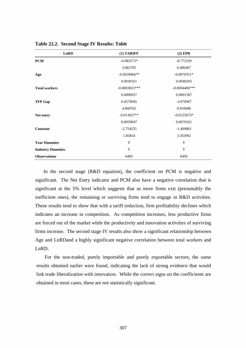
307

Table 22.2. Second Stage IV Results: Tobit

LnRD (1) TARIFF (2) EPR

PCM -6.083573* -8.772339

3.682705 6.686467

Age -0.0059966** -0.0070351*

0.0030161 0.0040205

Total workers -0.0003815*** -0.0004406***

0.0000937 0.0001567

TFP Gap 0.4578945 -3.076967

4.868762 8.810686

Net entry -0.013027** -0.0125073*

0.0059947 0.0070161

Constant -2.754255 -1.409861

1.85854 3.355992

Year Dummies Y Y

Industry Dummies Y Y

Observations 6495 6495

In the second stage (R&D equation), the coefficient on PCM is negative and

significant. The Net Entry indicator and PCM also have a negative correlation that is

significant at the 5% level which suggests that as more firms exit (presumably the

inefficient ones), the remaining or surviving firms tend to engage in R&D activities.

These results tend to show that with a tariff reduction, firm profitability declines which

indicates an increase in competition. As competition increases, less productive firms

are forced out of the market while the productivity and innovation activities of surviving

firms increase. The second stage IV results also show a significant relationship between

Age and LnRDand a highly significant negative correlation between total workers and

LnRD.

For the non-traded, purely importable and purely exportable sectors, the same

results obtained earlier were found, indicating the lack of strong evidence that would

link trade liberalization with innovation. While the correct signs on the coefficients are

obtained in most cases, these are not statistically significant.

308

6. Conclusions and Policy Implications

6.1. Summary of Major Findings

The most recent literature on trade and growth shows that international trade

affects firms’ innovative activities through increased competition. As Licandro (2010)

noted, increasing evidence supports the claim that international trade enhances

innovation and productivity growth through an increase in competition. In the

Philippines, trade liberalization has been at the core of economic reforms. The increase

in competition arising from the removal of barriers to trade has presented both

opportunities and challenges to domestic firms to innovate and improve their

productivity. This paper has attempted to examine the link between trade liberalization

and innovation. What is the impact of the removal of barriers to trade on the firms’

innovative activities? Did the increase in competition arising from trade reforms lead

to increases in innovation?

Impulliti and Licandro (2009, 2010) introduced a framework where trade affects

both firm selection and innovation through the competition channel. Given an

oligopolistic environment, trade liberalization leads to an increase in the number of

firms in the domestic market which raises product market competition and lowers the

markup rate. The selection effect of trade operates through endogenous markups

resulting from oligopolistic competition among firms. The reduction in the markup rate

(or increase in competition) due to trade liberalization reduces profits, increases the

productivity threshold above which firms can profitably produce and forces the less

productive firms out of the market. Resources are reallocated from exiting firms to the

higher productivity surviving firms which innovate at a faster pace.

Without Net Entry indicator, both the IV and Tobit results show that for overall

manufacturing industry, trade liberalization affects innovation through competition. In

the first stage, Tariff is highly correlated with PCM while in the second stage, a

significant relationship between PCM and R&D is obtained. This suggests that reduced

profit (which implies high competition) is associated with increased R&D.

309

Controlling for firm entry and exit, the IV and Tobit results show generally the

same findings. With Tariff as trade indicator, trade liberalization has a strong positive

impact on competition while competition has a significant effect on R&D.

Firms have also been grouped based on their trade orientation intensity: nontraded,

purely importable, purely exportable, and mixed sector. It is in the latter sector where

trade is most intense. In general, the major results again confirm the importance of

market competition as the channel through which trade liberalization affects

innovation. Selection arising from competition also plays a role. These results are

highlighted in the mixed sector which is characterized by substantial imports and

exports of products in industries like motor vehicle parts and components, semi-

conductors, parts and supplies for radio, TV, communication, appliances and house

wares, garments, carpets and rugs, furniture, along with sugar, glass, chemicals,

cigarette, soap and detergents, iron and steel and drugs and medicines.

Based on IV regression, the key results in the mixed sector show a significant

positive effect of trade liberalization on innovation through competition. The same

results are obtained in both models with and without the Net Entry indicator. The

results tend to show that with a tariff reduction, firm profitability declines which

indicates an increase in competition. As competition increases, the productivity

threshold in which firms could operate profitably increases, hence less productive firms

are forced out of the market while more productive firms are allowed to continue their

operations. With competition, the productivity and innovation activities of the

surviving firms increase.

The Tobit results show a highly significant positive relationship between PCM and

Tariff as well as a significant positive relationship between PCM and EPR. In the first

stage, a highly significant positive relationship between PCM and Tariff is found. In the

second stage, a significant negative correlation between PCM and LnRD is found. The

Net Entry indicator and PCM also have a negative correlation that is significant at the

5% level. This suggests that as more firms exit (presumably the inefficient ones), the

remaining or surviving firms tend to engage in R&D activities. The results tend to

imply that with a tariff reduction firm profitability declines which indicates an increase

in competition. As competition increases, less productive firms are forced out of the

market while the productivity and innovation activities of surviving firms increase.

310

6.2. Some Policy Recommendations

Given the crucial role of competition in the relationship between trade liberalization

and innovation, it is important for the government to maintain the contestability of

markets. Contestability is the essence of effective competition; for as long as markets

remain contestable (when entry into a market is easy), we would expect large firms in

an oligopolistic environment to act independently, and monopolies to behave in a

competitive manner. If entry is easy and costless, the potential threat from imports or

from domestic competitors will make incumbent firms behave competitively.

It is important to note that the presence of market imperfections, such as abuse of

dominant position and other anti-competitive business practices, along with trade

barriers or government regulations, limit market entry and create inefficiencies leading

to reduced long-term growth. These weaken competition and prevent structural changes

from taking place, resulting in resources being tied to low-productivity industries.

Weak competition reduces the pressure on firms to adopt new technology or innovate,

resulting in low growth of productivity and a loss of competitiveness.

Philippine experience has shown that after two decades of implementing

liberalization and other market-opening policies, competition and productivity growth

remained weak not only due to the presence of structural and behavioral barriers to

entry, but also to the country’s inadequate physical and institutional infrastructure. Due

to the fundamental weakness of competition in many major economic sectors, the gains

from liberalization remained limited which slowed down the country’s economic

growth.

The results have a bearing on the possible impact of the government’s selective

protection policy on competition and innovation. This policy, which was adopted in

2003, increased the tariff rates on selected agriculture and manufacturing products

which has led to a sizeable proportion of products with tariff peaks. The paper’s

findings tend to suggest that an increase in tariffs will increase profitability and reduce

competition which would likely result in reduced innovation, holding all else equal.

The selective protection policy must thus be reviewed, given its likely negative impact

on competition and innovation and taking into account the current low level of R&D

spending and overall innovation activity in the country.

311

It is necessary to address the remaining barriers to market entry (and exit) such as

selective tariff protection and non-tariff measures in rice, sugar, automotive parts and

components and other manufacturing products. The government needs to veer away

from protectionist policies and mechanisms that intervene in the market and try to

decide and select which firms should survive and which ones would die. In the light of

the findings of this paper and the increasing globalization and economic integration that

make industries more mobile through production networks and supply chains, the

government should focus on designing an overall policy and strategy that would ensure

competition, innovation and the productivity growth of firms. Beginning in January

2010, the ASEAN Trade in Goods Agreement (ATIGA) where tariffs were reduced to

zero in a substantial number of products has been implemented. Whether this will lead

to more competitive markets in the Philippines depends not only on the overall trade

creation and trade diversion effects of the ASEAN Economic Community (AEC) but

also on the government strategy that will be put in place to help our industries face

increased competition from imports, and take advantage of opportunities such as bigger

export markets and increased foreign direct investment flows. Note also that there are

other important determinants of innovation including human capital, infrastructure, and

institutional factors that must be closely examined along with their interaction with

trade policy reform indicators.

312

References

Aghion, Philippe, Robin Burgess, Stephen Redding and FabrizioZilibotti (2005), ‘Entry Liberalization and Inequality in Industrial Performance’, Journal of the European Economic Association, Papers and Proceedings, 3(2-3): 291-302.

Aghion, P. and Robin Burgess (2003), ‘Liberalization and Industrial Performance: Evidence from India and the UK’.

Aghion, P., Nicholas Bloom, Richard Blundell, Rachel Griffith, and Peter Howitt (2002), “Competition and Innovation: An Inverted U Relationship’, Working Paper 9269. National Bureau of Economic Research. Cambridge, MA.

Aghion, P. and Peter Howitt (1999), Endogenous Growth Theory. Massachusetts Institute of Technology. US.

Aldaba, R. (2010), ‘Does Trade Protection Improve Firm Productivity? Evidence from Philippine Micro Data’, Paper submitted to ERIA in March 2010.

_______(2008), ‘Assessing Competition in Philippine Markets’, PIDS Discussion Paper 2008-23, Makati City.

Bloom, N., MirkoDraca, and J. Van Reenen (2010), ‘Trade Induced Technical Change? The Impact of Chinese Imports on Innovation, IT and Productivity’.

Blundell, R., R. Griffith, and J. Van Reenen. (1995), ‘Dynamic Count Data Models of Technological Innovation’, Economic Journal, 105(429):333-344.

Carlin, Wendy, Mark E. Schaffer and Paul Seabright (2004), ‘A Minimum of Rivalry: Evidence from Transition Economies on the Importance of Competition for Innovation and Growth’, Contributions to Economic Analysis & Policy 3(1): Berkeley Electronic Press.

Cororaton, C. (2002), ‘Technological Innovations in Japan and S&T Experiences in the Philippines Drawing Policy Lessons for the Philippines’, PIDS Research Paper Series No. 2002-04, Makati City, Philippines.

___________ (1999), ‘R&D Gaps in the Philippines’, PIDS Discussion Paper Series No. 99-16, Makati City, Philippines.

Creusen, H., B. Vroomen, H. van derWiel and F. Kuypers. (2006), ‘Dutch Retail Trade On The Rise?: Relation Between Competition, Innovation And Productivity’, CPB Document 137, CPB Netherlands Bureau for Economic Policy Analysis.

Domowitz, I., Hubbard & Petersen (1986), ‘The Intertemporal Stability of the Concentration Margins Relationship’, Journal of Industrial Economics, Vol. 35 (1):13-34.

Fernandes, A. and Caroline Paunov (2009), ‘Does Tougher Import Competition Foster Product Quality Upgrading?’.

Geroski,P. (1995), Market Structure, Corporate Performance and Innovative Activity. Oxford University Press. Oxford, U.K.

________. (1990), ‘Innovation, Technological Opportunity and Market Structure’, Oxford Economic Papers.42: 586-602.

313

Gilbert, R. (2006), ‘Looking for Mr. Schumpeter: Where Are We in the Competition-Innovation Debate?’, Innovation Policy and the Economy, Vol. 6: 159-215, The University of Chicago Press.

Gorodnichenko, Y., Jan Svejnar, and Katherine Terell (2009), ‘Globalization and Innovation in Emerging Markets’, Policy Research Working Paper 4808, The World Bank.

Griliches, Z. (1992), ‘The Search for R&D Spillovers’, Scandinavian Journal of Economics, 94:29-47.

Hall, R. (1988), ‘The Relation between Price and Marginal Cost in US Industry’, Journal of Political Economy, 96:921-947.

Hopman, C. and Hugo Rojas-Romagosa (2010), ‘The Relation Between Competition and Innovation: Empirical Results and Implementation into WorldScan’, CPB Memorandum Netherlands Bureau for Economic Policy Analysis.

Impulliti, G. and Omar Licandro (2009), ‘Trade, Firm Selection, and Innovation: The Competition Channel’, May 2009.

Licandro, O. and Antonio N. Ruiz (2010), ‘Trade Liberalization, Competition and Growth’, February 2010.

Macapanpan, T. (1999), ‘Private Sector Activities on R&D’, PIDS Discussion Paper No. 99-19, Makati City, Philippines.

Nickell, S.J. (1996), ‘Competition and Corporate Performance’, Journal of Political Economy, 104(4):724-46.

Organisation for Economic Co-operation and Development Secretariat (2007), Discussion Paper on Trade, Innovation and Growth. OECD, Paris.

Patalinghug, E. (2003), ‘The Philippine Innovation System: Structure and Characteristics’, PIDS Research Paper Series No. 2003-04, Makati City, Philippines.

Schumpeter, J. (1942), Capitalism, Socialism, and Democracy. New York: Harper.

Siotis, G. (2003), ‘Competitive Pressure and Economic Integration: An Illustration for Spain, 1983-1996’, International Journal of Industrial Organization, 21:1435-1459.

314

Appendix Appendix I: Price Cost Margin A.P Lerner (1933-34) defined PCM or Lerner index of monopoly power as:

equation (1a)

Where B is price cost margin, P is price, and MC is marginal cost. For a competitive

firm, P = MC and the Lerner index is equal to zero. For a monopolist, P>MC and the

Lerner index becomes positive and varies between 0 and 1.

The mark up ratio, a simple way of measuring the level of competition, is given by

the ratio of price to marginal cost of production by firms in an industry. This can be

written as:

equation (1b)

Where μ is the mark up ratio. This variable indicates the level of competition or market

power of firms in industries. When firms have market power, P>MC and mark ups are

greater than 1 in equilibrium. In perfect competition, P=MC. The price cost margin can

be easily mapped into the mark up ratio μ. Equation (6) can be rewritten as:

equation (1c)

  

P

MCPB

MC

P

B

1

1

315

CHAPTER 9

Trade Liberalization and Innovation Linkages

Micro-evidence from Vietnam SME Surveys

NGUYEN NGOC ANH

1

Development and Policies Research Center (DEPOCEN)

NGUYEN PHUONG MAI

Development and Policies Research Center (DEPOCEN), National Institute for Science and

Technology Policy and Strategy (NISTPASS)

NGUYEN DUC NHAT

Development and Policies Research Center (DEPOCEN)

NGUYEN DINH CHUC

Central Institute of Economic Management (CIEM)

Vietnam has long been pursuing its far-reaching trade liberalization program which has led to

rapid economic growth and poverty reduction. Innovation has long been considered an important

factor for creating and maintaining the competitiveness of nations and firms. This paper

investigates the impacts of trade liberalization on innovation activities by SMEs, the most dynamic

and important sector for Vietnam’s future economic development. Using the recently released

Vietnam Small and Medium Enterprise Survey, we find that innovation, as measured directly by

‘new products’, ‘new production process’ and ‘improvement of existing products’ are strongly

influenced by trade liberalization.

Keywords: Innovation, Export, Vietnam, SME, Trade liberalization

JEL Classification: D21, L23, O31, O32

1 The authors are solely responsible for the opinions expressed in this paper. We would like to thank participants at ERIA Workshops for their comments and suggestions. The data used in this paper are kindly provided by MOLISA. Financial support from ERIA is gratefully acknowledged. Corresponding author: Nguyen Ngoc Anh, Development and Policies Research Center (DEPOCEN), 216 Tran Quang Khai Street, Hanoi, Vietnam, email: ngocanh@depocen.org

316

Introduction

After 20 years of reform, Vietnam has put in place the fundamentals of a market

economy and actively participated in the globalization process by opening up the

economy to international flows of capital and trade in goods and services.2 The

emergence of the market-based economy with appropriate institutions, stable

macroeconomic environment and the support of the government for business

development have allowed Vietnam to (i) unlock the potential of the agriculture sector,

turning Vietnam from a food-hungry country to the world's third largest rice exporter3;

(ii) encourage the development of a vibrant domestic private sector; (iii) attract a large

amount of foreign investment; (iv) realize its comparative advantages and gain more

benefits from international trade. These factors underlie the economic success that

Vietnam has been achieving since the early 1990s. The country is now recognized as

being among the most successful developing countries in terms of economic growth and

poverty reduction.

As can be seen in Figure 1, during the period 1990–2008, the annual GDP growth

rate averaged more than 7 percent, and Vietnam’s growth rates today remain among the

highest the region. The average annual GDP growth was about 5-6 percent during the

period1990–91, climbing to and then staying at about 8 percent from 1992 to 1997.

GDP growth, however, declined between 1998 and1999, partly because of the Asian

crisis and the dissipation of the effects of reform. Since 2000, the economy has

regained its momentum. Its annual growth rate exceeded 7 percent—reaching 8.5

percent in 2007—then dropped back to an estimated 6.2 percent in 2008, owing to the

effects of the global recession. High and continuous GDP growth rates and successful

economic development from 2000 to 2008 have resulted in significant improvements in

the population’s welfare and in substantial poverty reduction. According to the

2 “Globalization” is a loaded concept and may mean different things to different people, in different contexts. From an economic perspective, it usually refers to the removal of barriers to the cross-border movements of goods, funds, personnel and information. The more easily such movements take place, the higher the degree of globalization. 3 Che et al. (2003) report that market reform leads to an increase in rice productivity, pointing to the importance of market competition, secured property rights and efficient use of resources. See http://www.crawford.anu.edu.au/degrees/idec/working_papers/IDEC03-7.pdf

317

Vietnam Household Living Standard Survey, the total poverty incidence declined from

58 percent in 1993 to 37 percent in 1998, 29 percent in 2002, 19.5 percent in 2004, and

16 percent in 2006 (SRV 2003; Nguyen 2009). In addition, improvements have been

made in other aspects of human welfare, such as the sharp rise in the percentage of

literate adults (to over 90 percent), longer life expectancy (over 70 years), and a lower

mortality rate for children less than five years old (40 per 1,000 live births in 2003).

Figure 1. Vietnam Trade Liberalization and Economic Development

Note: In 1992, Vietnam signed a trade agreement with the European Union (EU). In 1995, it joined ASEAN and committed to fulfill the agreements under AFTA by 2006. Vietnam applied for WTO membership in 1995 and became a member in 2007. In 1998, it became a member of the Asia-Pacific Economic Cooperation (APEC) and, in the year 2000, signed the Bilateral Trade Agreement with the United States (VN-U.S.BTA). This agreement came into force in December 2001. Recently, Vietnam has also joined regional integration clubs such as ASEAN-China Free Trade Area (2002) and ASEAN-Japan Comprehensive Economic Partnership (2003).

As a result of its effort to integrate into the global economy, Vietnam has

substantially liberalized its trade and investment regimes which have enabled Vietnam

to attract a large inflow of foreign direct investment (FDI) and witness trade expansion.

The process has created a growing and dynamic private sector consisting of mainly

small and medium enterprises. In the face of Vietnam's increased integration into the

318

world market, and particularly following the country's entry into the WTO at the end of

2006, the SMEs are having a great opportunity to expand by exporting to other markets.

But at the same time they are also facing tough competition on their door step.

According to endogenous growth theory, technological innovation is important to

the “sustained” growth of an economy (Romer, 1986; Lucas, 1988).4 Like many other

emerging market economies/countries, globalization brings about opportunities and also

pressures for Vietnamese domestic firms to innovate and improve their competitive

position. Many of these pressures and opportunities operate through increased

competition from, and linkages with, foreign firms and exposure to the international

market. The major problem is that the Vietnamese private sector, and small and

medium enterprises in particular, is not yet sufficiently competitive. As a result, most

companies cannot yet withstand the competitive pressure resulting from liberalization

and the opening to the world market, not to mention exporting to the world market. The

key question facing policy makers is how to improve the competitiveness of Vietnam’s

enterprises, especially the SME sector which accounts for a large part of the economy.

Among the many initiatives being proposed to improve the competitiveness of

Vietnam’s SMEs, innovation policy has attracted attention not only from policy makers,

but also from researchers and the business community (Nguyen et al., 2008). These

initiatives are based on the assumption that innovation can affect a firm’s

competitiveness and hence export status by increasing productivity (and reducing costs),

and by developing new goods for the international market.5

In this paper, we use the conceptual frameworks of a number of recently developed

models (e.g. Sutton, 2007) to examine the determinants of innovation by Vietnamese

SMEs in the context of increased competition and linkages resulting from trade

liberalization. Specifically, we focus on the effect of competition and transfer of

capabilities stemming from globalization, which may be brought about through various

channels, including the spillover effects of FDI, exposure to international trade, and

4 The acquisition of knowledge and intelligence, technological innovation and human capital accumulation are the main reasons for the economic growth of the newly industrialized economies (Bassanini and Scarpetta, 2002; Hu & Mathews, 2005; Mueller, 2006, Nguyen and Nguyen 2010). 5 This can be analyzed in the context of firms that compete in markets with differentiated products. Firms sell low-quality goods in domestic markets, but if they want to sell abroad then they must upgrade technologies to produce high-quality goods.

319

increased competitive responses by domestic firms. After briefly reviewing the

previous studies in section 2, we present our data and econometric specification in

section 3. We discuss our empirical results in section 4 while we conclude in section 5.

Trade Liberalization and SME Development in Vietnam

The evolution of globalization for Vietnam in the last 20 years is also illustrated in

Figure 1. Vietnam has substantially liberalized its trade and investment policies since

the late 1980s. During the early years of economic reform, Vietnam liberalized its trade

regime through signing trade agreement with around 60 countries. It has also

implemented a preferential trade agreement with the European Union since 1992. Later

on, the country actively sought membership of regional and global organizations.6

Vietnam has been a member of the Association of South East Asian Nations (ASEAN)

since June 1995 and the Asia Pacific Economic Co-operation (APEC) since 1998. In

2000 Vietnam signed a historic comprehensive trade agreement with the USA to

normalize trade relations between the two countries. Recently, Vietnam has also joined

regional integration clubs such as ASEAN - China Free Trade Area and ASEAN-Japan

Comprehensive Economic Partnership. Most recently, in 2007 Vietnam became the

latest member of the World Trade Organization.

This process of trade regime liberalization has led to increased trade flows, and in

particular export, for the country. In a recent paper, Abbott et al. (2009) observe that

each time Vietnam reached a significant bilateral agreement, trade flows with that

partner surged. Vietnam has also seen a steady growth in its international trade over the

period. The average growth rate of export and import is around 20%. The total value of

international trade over the GDP, which is one indicator of the openness of an economy,

reached 150 per cent in 2007, up from 61 per cent in 1994. The structure of import and 6 International integration processes picked up from the early 1990s after the collapse of the Berlin wall, and Vietnam lost its traditional markets in Eastern Europe and The Soviet Union in the late 1980s. The US trade embargo against Vietnam was only lifted in 1994, and the relationship with the US was normalized in 1995. Another important achievement and event is that since 1993 Vietnam has begun to receive overseas development assistance (ODA) from foreign governments which have contributed to the substantial increase in financial resources for Vietnam’s development.

320

export has substantially changed in comparison with the previous period. Vietnam has

exported oil, various manufacturing and agriculture-processing products, and imported

not only consumption goods, but mainly raw materials for domestic production and

initially progressive techniques and technology to promote the growth and efficiency of

the economy. The composition of Vietnamese exports has gradually reflected the

success of the industrialization process. The share of manufactured products,

particularly labor intensive products like textiles and garments, footwear, and seafood,

has been increasing and replacing the traditional agricultural products. In 2005, the

share of manufactured handicraft products alone accounted for more than 40 per cent of

total export value (CIEM 2005).

The Law on Foreign Direct Investment (FDI) was first promulgated in 1987 and

later amended in 1990, 1992, 1996 and 2000 which helped Vietnam to attract a large

volume of foreign capital when domestic savings were insufficient to meet investment

needs. By 1987, the private sector virtually did not exist in Vietnam. By allowing

foreign direct investment, Vietnam in effect imported/implanted the private sector of its

own for the first time after the unification of the country. Since then, FDI has indeed

become an integrated part of the Vietnamese economy and an important factor in

Vietnam’s economic growth during the 1990s. In order to create a more level playing

field and to ensure that its laws allowed for national treatment for FDI enterprises prior

to Vietnam’s 2006 accession to the World Trade Organization, in 2006 Vietnam

promulgated two important laws, the Investment Law and the new Enterprise Law7,

creating a corporate law regime that applies to both foreign and domestic enterprises.8

Thanks to the progressively liberalized regulations toward FDI, the FDI sector has

now become an important part of the national economy. After a slowdown in FDI

inflow in the aftermath of the Asian financial crisis, recently, new large FDI inflows

have emerged, in part as a result of reforms committed to as part of WTO accession that

7 Specifically, on November 29, 2005, the National Assembly of Vietnam adopted the Law on Investment No. 59/2005/QH11 (“New LOI”) and Law on Enterprises No. 60/2005/QH11 (“New LOE”) which apply to all enterprises established by domestic and/or foreign investors. 8 Besides FDI, Vietnam also started to receive the ODA from international donors in 1993 and the amount committed and disbursed has been increasing since then. These capital sources constitute a positive assistance to infrastructural construction such as transport and communication, information, agricultural and rural development, public health, education and training, administrative reform, legislation, and structural reform.

321

relaxed rules restricting FDI, making Vietnam a more attractive FDI destination. The

sudden increases in the share of the FDI sector during the period 2007-2008 can be

partly explained by the WTO accession of Vietnam which generated hype among

foreign investors about the prospect of doing business in Vietnam.9 Although Vietnam

has been successful in attracting FDI in recent years, the real benefits from FDI still

seem controversial. Previous studies have found little evidence of technical spillover

from FDI enterprises to local counterparts (Nguyen et al., 2008). In addition, the

country has become heavily dependent on FDI capital as an important source of input to

sustain economic growth.

As discussed above, the last 20 years have witnessed comprehensive reforms being

implemented in Vietnam which, together with an open-door policy to attract foreign

direct investment and trade liberalization with the culmination of WTO accession in

2007, have created a growing dynamic private sector in Vietnam. However, the vibrant

emergence of the private sector and SMEs is a recent development in Vietnam. When

Vietnam opened up to outside world under its Doi Moi, starting with some timid

reforms, the Vietnamese government officially granted its recognition of private

enterprises in the early 1990s with the introduction of the Company Law and the Law

on Private Enterprises. Despite this early official recognition for the private business

sector, private enterprises developed slowly with only 39,600 enterprises established

during the 1990s. Major growth in the formal private sector came with the 1999

Enterprise Law, which gave a much clearer legal status for the private sector. Since the

Law became effective on 1 January 2000 the country has experienced a boom in private

SMEs. They have now become a strong part of the national economy and have made a

significant contribution to economic growth, job creation, exports and poverty

reduction.

Small and medium-sized enterprises (SMEs) are a very heterogeneous group 10 and

their definition varies by country. Usually the definition is based on the number of

9 Vietnam requires registration of intended FDI, and not all of those registrations are implemented. 10 SMEs operate in a wide array of business sectors, ranging from handicraft producers for village markets, coffee shops on the street, and Internet cafés in a small town to small sophisticated engineering or software firms selling to overseas markets and a medium-sized manufacturers supplying inputs to multinational automakers in both domestic and foreign markets.

322

employees, and value of sales and/or value of assets. The most commonly used criteria

among a large number countries (both developed and developing) are the number of

employees, for which the upper limit of number of employees in SMEs is set at between

200 and 250, with a few exceptions such as in Japan (300 employees) and the USA (500

employees).11 In Vietnam, SMEs are defined using two criteria: number of employees

and registered capital. According to Vietnamese laws and regulations (Government

Decree 90/2001/ND-CP), Vietnamese SMEs are legally defined as

“independent production and business establishments” with registered capital not

exceeding VND 10 billion12 or annual labor not exceeding 300 people. Based on this

definition, the SMEs in Vietnam account for 97 percent of the total number of

Vietnamese enterprises (calculated based on annual labor) or some 85 percent

(calculated based on capital), given by the latest statistical data of the Vietnam General

Office of Statistics.

Economic reform during the last decades has directly stimulated the development

and performance of Vietnamese SMEs. As can be seen in Table 1 which classifies

SMEs by the number of employees, the SMEs account for 97 percent of the total

number of firms in 2008, an increase from 92 percent in 2000. The average growth rate

of the SMEs under this classification was 23 percent in contrast with the average rate of

just seven percent for the large enterprises. Under the capital classification criteria used

in Table 2, the SME sector also account for 96% of the total number of firms with an

average growth rate of 22 percent. In contrast to the employment classification, the

SMEs' growth rate is still higher than 20 percent but two percentage point lower than

the large enterprises. Vietnamese SMEs have been outperforming other enterprises in

exploiting Vietnam’s comparative advantage in labor-intensive production (Harvie,

2001).

11 See Promoting SMEs for Development http://www.oecd.org/dataoecd/6/7/31919278.pdf 12 At current exchange rate equivalent to around USD 450,000 decreasing from USD 600,000 due to the Dong’s depreciation.

323

Table 1a. Distribution of Small and Medium Enterprises 2000-2008 (by Employees)

Total Number of Firms (including

SME) SME

Micro Enterprises

Small Enterprises

Medium Enterprises

Large Enterprises

2000 42288 92% 54% 34% 4% 8% 2001 51680 93% 54% 35% 4% 7% 2002 62908 93% 53% 37% 4% 7% 2003 72012 94% 51% 39% 3% 6% 2004 91756 95% 53% 38% 3% 5% 2005 112950 96% 56% 37% 3% 4% 2006 131318 96% 61% 32% 3% 4% 2007 155771 96% 61% 33% 3% 4% 2008 205689 97% 62% 33% 2% 3%

Table 1b. Growth Rate of Firms 2001-2008

Total Number of

Firms (including SME) SME

Average Micro

Enterprises Small

Enterprises Medium

Enterprises Large

Enterprises

2001 51680 23% 23% 25% 7% 9% 2002 62908 22% 18% 29% 16% 15% 2003 72012 15% 12% 20% 9% 6% 2004 91756 29% 33% 25% 16% 6% 2005 112950 24% 29% 18% 11% 4% 2006 131318 17% 26% 3% 7% 5% 2007 155771 19% 19% 19% 19% 8% 2008 205689 33% 33% 34% 10% 6%

Source: GSO. Calculation by authors. Classification by number of employees. Table 2a. Distribution of Small and Medium Enterprises 2000-2008 (by Capital)

Total number of

Firms (including SME) SME Small Enterprises Medium Enterprises Large Enterprises

2000 42288 97% 88.8% 7.9% 3.3% 2001 51680 97% 89.2% 7.6% 3.1% 2002 62908 97% 89.0% 7.8% 3.1% 2003 72012 97% 89.0% 7.8% 3.2% 2004 91756 97% 89.3% 7.6% 3.1% 2005 112950 97% 89.7% 7.4% 3.0% 2006 131318 97% 89.6% 7.4% 2.9% 2007 155771 96% 87.8% 8.6% 3.6% 2008 205689 96% 86.4% 9.9% 3.7%  

 Table 2b. Growth Rate of Firms 2001-2008 (by Capital)

Total number of

Firms (including SME) SME Small Enterprises Medium Enterprises Large Enterprises

2001 51680 22% 23% 18% 16% 2002 62908 22% 21% 25% 22% 2003 72012 14% 14% 14% 16% 2004 91756 28% 28% 24% 23% 2005 112950 23% 24% 19% 19% 2006 131318 16% 16% 17% 15% 2007 155771 18% 16% 37% 46% 2008 205689 32% 30% 52% 34%

Source: GSO. Calculation by authors. Classification by capital.

324

Table 3 presents a breakdown of Vietnamese SMEs, categorised in terms of

ownership, for the period 2000-2008. The first row shows the total number of SMEs.

The data indicates that, after a period of 9 years up to 2008, the numbers of SMEs

increased by more than five times from 39897 in 2000 to 201590 in 2008. In the last

three rows, the number of SMEs is computed as a share of each ownership type on total.

The ownership structure of SMEs indicates that most SMEs are non-state owned. The

number of state-sector SMEs decreased due to the progress of privatization. In 2000,

nearly 11% of SMEs were state owned versus only 3% foreign-owned. In 2008, the

SMEs in these two ownership sectors represent only 3.3 percent of the total number.

Table 3. Number and Ownership Structure of Vietnamese SMEs 2000-2008

Year 2000 2001 2002 2003 2004 2005 2006 2007 2008

Total 39897 49062 59831 68687 88222 109336 127593 151780 201580

Ownership structure

State owned enterprise 10.5 7.6 6.1 4.6 3.4 2.4 1.9 1.5 1.1

Non-state enterprise 86.4 89.0 90.9 92.5 93.9 94.9 95.5 95.9 96.7

Foreign investment enterprise 3.0 3.4 3.0 2.9 2.7 2.6 2.6 2.5 2.2

 

Unit: % Source: Author’s elaboration based on Enterprise Census 2000-2008 of GSO of Vietnam.

Table 4 presents the percentage of the total number of firms in Vietnam which are

SMEs. The first row shows the share of total SMEs on total firms. The data shows that

almost 98 percent of the total number of existing firms in Vietnam are SMEs. Broken

down into type of ownership, the last three rows indicate the share of SMEs in each

ownership sector. The fact is that SMEs constitute an overwhelming share of the

private sector in Vietnam (99%). Share of SMEs in foreign owned firms (joint venture

or 100% foreign owned) decreased slightly, but still made up more than three quarters

of the firms in that sector. Share of state-owned SMEs decreased due to privatization.

325

Table 4. Share of Vietnamese SMEs in Total Firms by Type of Ownership

Year 2000 2001 2002 2003 2004 2005 2006 2007 2008

Total 94.3 94.9 95.1 95.4 96.1 96.8 97.2 97.4 98.0

Ownership structure

State owned enterprise 72.8 70.1 67.7 64.9 64.4 65.5 66.3 67.0 67.1

Non-state enterprise 98.5 98.5 98.5 98.4 98.6 98.7 98.8 98.8 99.1

Foreign investment enterprise 79.5 81.8 78.0 76.4 76.8 77.6 77.3 77.7 79.2

Unit: %. Source: Author’s elaboration based on Enterprise Census 2000-2008 of GSO of Vietnam.

Table 5 presents the sectoral structural change of Vietnamese SMEs. The data

shows that most of structural changes occurred in 2000-2008 within the fishing and

services sectors. The number of SMEs working in the fishing industry decreased

remarkably during the last nine years. Less than 1% of SMEs remain in fishing

(compared to about 6% in 2000). In contrast, more SMEs engage in the service sector

(about 21% in 2008 compared to 15.4% in 2000).

Table 5. Sectoral Structure of Vietnamese SMEs

Year 2000 2001 2002 2003 2004 2005 2006 2007 2008

Total (100%) 39897 49062 59831 68687 88222 109336 127593 151780 201580

Agriculture and forestry 1.96 1.48 1.37 1.15 0.99 0.86 0.75 0.68 3.54

Fishing 6.14 5.21 4.01 2.13 1.53 1.24 1.02 0.85 0.67

Mining and quarrying 0.86 1.16 1.34 1.39 1.27 1.11 1.02 1.07 1.05

Manufacturing 22.93 22.38 21.97 21.84 20.90 19.98 19.24 18.80 17.78 Electricity, gas and water supply 0.25 0.27 0.28 0.34 1.64 2.18 1.98 1.83 1.53

Construction 8.89 10.54 12.02 13.22 13.23 13.39 13.48 13.46 13.73

Trade 43.48 41.81 41.08 41.03 40.67 40.66 41.00 40.41 40.17

Services 15.48 17.15 17.93 18.91 19.79 20.60 21.51 22.90 21.53

Unit: %. Source: Author’s elaboration based on Enterprise Census 2000-2008 of GSO of Vietnam.

SMEs in Vietnam have an important role to play in the country’s economic

development and industrialization process. The performance of SMEs can be observed

though the state, non-state (largely comprising of SMEs) and foreign-owned sectors.

Regarding GDP contribution, according to CIEM (2005), in 2005 the state-sector firms'

contribution to GDP at current prices was almost the same as it was in 2000 (38.42% vs.

326

38.52% respectively). Non-state-sector contribution to GDP reduced from 48.2% in

2000 to 46.03% in 2005. As a result, the foreign investment sector contribution

increased (15.89% in 2005 vs. 13.27% in 2000).13 CIEM (2005) also reported the

investment behavior by ownership. Interestingly, share of non-state-sector investment

increased remarkably, with 32.2% of total 2005 investment versus 22.6% in 2000. This

implies that the private sector, or SMEs, are now paying more attention to investment

into their production. Hansen (2006) studied the determinants of growth and survival of

SMEs. A study, which was based on a panel data of Vietnamese SMEs from 1990 to

2000, shows that innovation has positive and significant effect on survival of SMEs.

The development of SMEs is limited in many aspects, especially by market

constraints and by SMEs’ internal limitations, including capital shortage,14 old

equipment, outdated technology, and lack of skills and management experience 15(Webster and Taussig, 1999) and also by lack of appropriate government support.16 In

Vietnam, SMEs have received comparatively little support and attention. Until now, the

most comprehensive document that lays out the details of the government action plan to

develop the SME sector is the Decision No: 236/2006/QD-TTg on the 5-year SME

development plan 2006-2010 by the Prime Minister, issued on October 23, 2006. 17

Though some legal documents have been issued to support the SMEs, in practice they

are not yet fully implemented. The recent Decree 56/2009/ND-CP on SME

development support in 2009, for example, enumerates the types of support SMEs can

receive from the government, but does not provide guidance on how to actually receive

that support.

13 More recent estimates suggest that the SMEs contribute about 45% of Vietnam’s GDP. http://cab.org.in/CAB%20Calling%20Content/Financial%20Cooperatives%20in%20India%20-%20Where%20are%20the%20Members/Innovative%20Ways%20in%20Financing%20SMEs.pdf 14 http://www.devoutreach.com/mar03/article/tabid/1373/Default.aspx 15 Modern corporate governance practices, such as those applicable in OECD countries are not yet fully adhered to by Vietnamese private SMEs. 16 http://www.adb.org/Media/Articles/2010/13364-vietnam-sme-reforms/ 17 http://www.business.gov.vn/uploadedFiles/Decision%20236-2006.pdf

327

A Literature Review

Successful innovation in new products and processes is increasingly being regarded

as the central issue in economic development (Porter, 1998).18 The concept of

innovation was first studied by Schumpeter (1943) which was later developed by

generations of economists into what now can be referred to as “innovation theory”

thanks to the pioneering work of Nelson and Winter (1982), Dosi (1984) and Pavitt

(1984). Historically, innovation literature was focused on the role of internal research

and development (R&D) on firm innovation (Griliches, 1979). However, despite the

fact that R&D is often a cornerstone of an effective innovation strategy, internal R&D

expenditures played only a partial role in firm innovation rates.19 It is now increasingly

recognized that the ability to exploit external knowledge is critical to firm innovation

(Cohen and Levinthal, 1990; Henderson and Cockburn, 1994; Teece et al., 1997).

Traditionally, only those firms involved in R&D activities for new processes and

products are considered technologically innovative firms.20 But Mansfield (1968)

suggests that both the firm that introduces new equipment in the market and the firm

that first uses it are considered innovative. De Propris (2002) separates the innovation

into four types: product, process, incremental and radical innovation. Relevant to our

study, according to this author (De Propris, 2002) product innovation corresponds to the

introduction to the market of new or improved products, whereas process innovation

relates to the sequences and nature of the production process. Process innovation is

18 According to Rothwell (1994) there are five generations of innovation models. The first generation model of innovation is also known as “technology push”. The second generation innovation model – “need pull” – implies a shift toward a market/customer focus. The third generation is called the “coupling model” - a coupling of the push and pulls models. The fourth generation model of innovation, the “integrated model” suggests the coupling of marketing and R&D activities, together with strong supplier linkages and close coupling with leading customers. Finally, the fifth generation innovation is the “networking model”. 19 There is a large amount of literature on R&D and firm performance commonly referred to as the CDM models. However, the relationship between a firm’s performance and R&D spending is often imperfectly understood. 20 Molero et al. (1998) characterize them as firms that execute activities on a regular basis, formally or informally, pursuing either the creation of new product and process technologies or their improvement, in order to obtain results –quantitative or qualitative- that could increase their competitive capacity against other firms that work in the same market, or open for them new markets, that is, supporting the growth of the firm.

328

often more difficult to detect but it is very important, especially for buyer-supplier

transactions. Both radical and incremental innovations can be either in product or

process.21

There are numerous studies on the process of innovation itself (i.e the process

leading to innovation) as its measurement is critical for both practitioners and

academics. Yet the literature is characterized by a diversity of approaches, prescriptions

and practices that can be confusing and contradictory. It is, however, generally believed

that the innovation process consists of a complex sequence of decisions. Examples

include the CDM model literature structuring the firm’s decisions on how, and how

much to innovate in a multi-stepped process. According to De Propris (2002), it seems

that the idea that innovation is a linear and sequential process proceeding through

specific steps has been replaced by a systemic approach to innovation. Edquist and

McKelvey (2000) and Lundvall (1992) argue that the innovation process should rather

be considered as a circular and complex system embracing interactive elements.

Faced with increasing international competition, innovation has become a central

focus in firms’ long-term strategies. Firms competing in global markets face the

challenges and opportunities of change in markets and technologies. According to

Veugelers and Cassiman (1999), one important aspect within innovation management is

the optimal integration of external knowledge, since innovation increasingly derives

from a network of companies interacting in a variety of ways.

A large volume of literature exists on the expected impact of trade liberalization on

domestic economic performance. In general, there is consensus on the fact that trade

openness leads to economic growth beyond that expected when no policy change occurs

(Rodrik 1999). It is generally believed that trade liberalization should be beneficial for

the domestic economy as well as the world as a whole. The reasons behind this include

greater consumer welfare despite any loss in fiscal revenue, greater access to

technology, the dynamic effects of competitiveness, inflows of investment, and

21 Fernández (2005) suggests that a radical innovation occurs when the technological knowledge needed, in order to exploit it, is very different of the already existent knowledge while incremental innovation refers to improvements due to use or experience; it can often take the form of smaller enhancements around major radical innovations. Freeman and Perez (1988) argue that the incremental innovation is crucial for firms’ productivity growth even though it is often underestimated in comparison to radical innovation.

329

improved resource allocation; access to better technologies, inputs and intermediate

goods; economies of scale and scope; greater domestic competition; availability of

favorable growth externalities like transfer of know-how, and many others.

At the firm level, trade liberalization could affect domestic enterprises and their

innovation. Increased competition: lower import barriers (tariffs, quotas and other non-

tariff barriers) would lead to increased foreign competition in the domestic market

which will force inefficient domestic firms to try to improve their productivity by

eliminating waste, exploiting external economies of scale and scope, and adopting more

innovative technologies, or they may shut down. Lower production costs due to

cheaper imported inputs which allow them to compete more effectively both against

imports in domestic markets and in export markets. Another strand of the literature

emphasizes the importance of international exposure through exporting as a source of

new knowledge accumulation. Being exposed to international competition, the

exporting firms can acquire important new knowledge through the process of learning-

by-exporting. In addition, international competition can also be a stimulus for the firm

to innovate for itself. Girma et al. (2004) report that exporters are more productive and

they do select themselves in exporting although they also report that exporting increases

a firm’s productivity.

As with trade liberalization, investment liberalization also has positive and negative

impacts on domestic firms and the SMEs. Sutton (2007) develops an industrial

organization model to explain the impact of trade liberalization on the behavior of firms

in the emerging market economies. The model assumes that a firm’s competitiveness

depends not only on its productivity but also on the quality of its product, with

productivity and quality jointly determining a firm’s “capability.” Sutton’s model

(2007) predicts that after an initial shakeout, firms in emerging markets will strive to

adjust by raising their capabilities, which may be improved by the vertical transfer of

capabilities to the emerging market economies through the supply chain of

multinational enterprises (MNEs). With the characteristic of public goods, knowledge

and technologies that MNEs bring along when they invest abroad could have long-run

impacts on the host country through the externality generated as suggested in

endogeneous growth models (Grossman and Helpman 1991, Lucas 1988, Romer 1990).

330

It is commonly recognized that MNEs possess more advanced technology. When

MNEs choose to penetrate a foreign market through direct investment, they are likely to

bring along more sophisticated technology and superior managerial practices. These

give them a competitive advantage over indigenous firms which tend to be more

familiar with consumer preferences, business practices, and government policies in the

host country market (Blomstrom and Sjoholm, 1999). It is possible that a portion of the

technologies and experiences transported by MNEs will be diffused from their affiliates

to the indigenous establishments in the host economy. Business associations with

MNEs provide important learning opportunities for the domestic firms. They could

reduce the costs of innovation and imitation for local firms, which will in turn speed up

productivity improvement (Helpman, 1999). FDI may raise productivity levels of

domestic firms in the industries which they enter by improving the allocation of

resources in those industries. The presence of multinationals, together with their new

products and advanced technologies, may force domestic firms to imitate or innovate.

The threat of competition may also encourage domestic firms which might otherwise

have been laggards to look for new technology. Another route for the diffusion of

technology is the movement of labor from foreign subsidiaries to locally-owned firms.

For example, local firms may learn to imitate a new process or improve the quality of

their product through observation, interaction with foreign managers in business

chambers, and from former employees of foreign multinational enterprises (MNEs).

Local firms may also benefit from the entry of new professional services or suppliers as

a result of the MNE entry. Foreign firms may act as catalysts for domestic suppliers to

improve the quality or time efficiency of their goods or services by demanding higher

standards. On the other hand, foreign firms may have a negative effect on domestic

firms’ output and productivity, especially in the short run, if they compete with

domestic firms and “steal” their market or their best human capital. As domestic firms

cut back production they may experience a higher average cost as fixed costs are spread

over a smaller scale of production (Aitken and Harrison, 1998).

331

Data and Econometric Methodology

In this paper, we use the Vietnam Small and Medium Enterprise Survey conducted

in 2007 and 2009 to investigate the link between innovation activities and exporting.

The survey has been conducted four times: in 1991, 1997, 2002, 2005, 2007 and 2009

by the Ministry of Labor, Invalid and Social Affairs (MOLISA) and the Stockholm

School of Economics, and in 2005 by MOLISA and University of Copenhagen.

Although the SME survey is a longitudinal survey, we only have access to the data in

2005, 2007 and 2009. In our study, we chose to focus specifically on 2007 and 2009

data as the period under study is the period that Vietnam experienced increased trade

liberalization.22 The SME survey was meant to be a national representative survey, and

was conducted in ten provinces in Vietnam. In all areas covered by the survey, the

sample was stratified by ownership to ensure that all types of non-state firms were

included. The SME survey is a rich dataset, containing a battery of information about

firms’ characteristics including enterprise dynamics and growth, bureaucracy,

informality, tax, employment, education, social insurance, innovation, export,

investment and finance.

In Vietnam, the survey is the only source of data that contains innovation

information for enterprises in general, and SMEs in particular. An important advantage

of our data is that firms self-report various types of innovation activity. The survey

distinguishes between whether the firm introduced new products (product innovation),

improved existing products (product modification) or introduced new production

process/new technology (process innovation). These are the measures of innovation we

used in this paper. 23

22 While data from previous waves are not available, the SME survey in 2002 did not distinguish between product vs. process innovation. 23 Most studies on innovation use patent data or R&D expenditures, which are problematic. Patents are generally viewed as having several weaknesses: 1) patents measure inventions rather than innovations; 2) the tendency to patent varies across countries, industries and processes; and 3) firms often use methods other than patents to protect their innovations (such as technological complexity, industrial secrecy, and maintaining lead time over competitors). Using R&D expenditures may also be problematic because not all innovations are generated by R&D expenditures, R&D does not necessarily lead to innovation, and formal R&D measures are biased against small firms (Michie, 1998; Archibugi and Sirilli, 2001). Perhaps most important for the purposes of this paper is that in

332

For empirical analysis, basically, we estimate the following equation

''' spilloverncompetitioZInnovation (1)

where Innovation is an indicator taking value of 1 if firm i is an innovator in the survey

year and 0 otherwise, Z is a vector which includes a firm’s characteristics such as firm

size (numwork) proxied by the number of workers, firm age (lnfirmage), skill of the

labor force (skillratio), capacity utilization (over_cap). Regional dummies and ε is an

error term. As the dependent variable is a binary response variable, the equation (1) is

estimated as a probit or logit model. As discussed above, our data allows us to

distinguish between product innovation, process innovation and product modification,

Innovation in (1) is a generic measure of innovation. In particular, in the empirical

investigation, we consider three measures of innovations:

Product Innovation: This is a dichotomous variable that takes the value 1 when

the firm introduces new products in the survey year; and 0 otherwise.

Process Innovation: This is a dichotomous variable that takes the value 1 if the

firm introduces new production processes/new technology; and 0 otherwise.

Product modification: This is a dichotomous variable that takes the value 1 if the

firm introduces any major improvement to existing products or changed

specification in the survey year; and 0 otherwise.

The SME survey data also allow us to capture the degree of competition faced by

each firm in various ways. Firms that are able to charge a larger markup are deemed to

have less competition. We are able to observe the pricing strategy of individual firms,

i.e. if they price their products/services according to their competitors (com_price). We

are also able to capture the effects of Foreign Competition (foreign_com) with a

dummy variable. As discussed above, foreign firms can spur innovation among

domestic firms through competition but they can also directly transfer capabilities. The

SME survey also permits us to capture in various ways the extent to which there may be

a spillover from foreign firms to domestic firms. We use three variables to capture the

linkages and exposure to foreign firms and international trade. In particular we use the

emerging-market economies these types of innovations are less likely to be observed as firms are expected to engage more in imitation and adaptation of already created and tested innovations, rather than in generating new inventions, and are less likely to expend resources on R&D.

333

percentage of sales to FDI firms (sale_mne), the share of inputs imported

(input_import), and whether a firm exports (export).

The argument for including firm size (numwork) is that large companies have

more resources to innovate and can benefit from economies of scale in R&D production

and marketing. Capacity utilization has been found to be a strong predictor of

innovations (Becheikh et al., 2006), the effect of capacity over-utilization (over_cap)

on innovation is a priori indeterminate. If firms are too busy fulfilling demand, they

may be more interested in extending their current capacity than finding new ways of

producing goods and services. At the same time, if firms are at capacity they may need

to innovate. The skill level of the labor force (skillratio), captures the human capital

available within the firm. This variable might be expected to be positively correlated

with innovation as it reflects the involvement of workers in R&D and more skilled

workers are able to give feedback to the firm on how to improve a product. Age of the

firm in number of years since the firm began operations (lnfirmage) is included because

older firms developed routines that are resistant to innovation and/or older firms will

accumulate the knowledge necessary to innovate. We report in Appendix 1 a detailed

description of the variables.

Empirical Results

The estimation results for 2007 and 2009 are presented in Table 6 and 7

respectively. Many interesting findings are contained in these two tables that we will

now discuss. We first focus on the competition effects. As can be seen in Table 6, the

effects of competition, both domestic and international, have important impacts on

innovation activities. The competitors' pricing (com_price) has a positive impact on

product innovation but not on process innovation or product modification. But foreign

pressure (foreign_com) also had positive impacts on all kinds of innovation activities in

2007. Sales to MNEs lead to improvement in the innovation activities of domestic

firms in all aspects (i.e. new products, new process, and product improvement). In

2009, however, the results are a bit different. Although pressure from price competition

334

(com_price) helps to improve innovation in terms of product

modification/improvement, it has no effect on product innovation and process

innovation. However, still resembling the effect in 2007, foreign competition pressure

helps firms to improve their innovation activities in terms of process and product

improvement, not new product innovation. Different from the results in 2007, sales to

MNEs and imported inputs seem to lose their importance. The estimated parameters are

not statistically significant. However, the estimated effect of exporting is still

statistically significant.

Table 6. Estimation Results for 2007

New Product New Process Product Modification

 Coef.

Std. Err.

P>z Coef. Std. Err.

P>z Coef. Std. Err.

P>z

sale_mne 0.01* 0.00 0.08 0.01* 0.00 0.01 0.00 0.00 0.71

input_import 0.00 0.00 0.66 0.00 0.00 0.32 0.00 0.00 0.72

over_cap -0.25* 0.14 0.07 -0.14 0.09 0.13 -0.23** 0.07 0.00

lnfirmage -0.16 0.08 0.04 -0.14** 0.05 0.01 -0.13*** 0.04 0.00

skillratio 0.08** 0.06 0.14 -0.04 0.05 0.42 -0.19*** 0.04 0.00

export 0.41** 0.18 0.02 0.26** 0.13 0.04 0.42*** 0.13 0.00

com_price 0.21* 0.12 0.09 -0.08 0.10 0.41 -0.13 0.08 0.12

numworker 0.00* 0.00 0.07 0.00*** 0.00 0.00 0.00*** 0.00 0.00

foreign_com 0.10 0.10 0.29 0.29*** 0.07 0.00 0.32*** 0.06 0.00

HN 0.53 0.17 0.00 0.43 0.10 0.00 0.50 0.09 0.00

Haiphong 1.10 0.16 0.00 -0.02 0.13 0.86 0.43 0.11 0.00

Hatay 0.38 0.17 0.03 0.19 0.10 0.06 0.21 0.09 0.02

Longan 0.89 0.19 0.00 0.09 0.15 0.57 0.02 0.13 0.85

Phutho 0.35 0.20 0.08 -0.51 0.15 0.00 -0.08 0.10 0.43

Quangnam 0.57 0.21 0.01 0.03 0.14 0.83 -0.07 0.12 0.58

Nghean 0.35 0.18 0.05 -0.31 0.12 0.01 0.21 0.09 0.02

Khanhhoa 0.08 0.33 0.81 -0.28 0.20 0.16 -0.44 0.16 0.01

Lamdong 0.53 0.24 0.03 0.14 0.17 0.43 0.42 0.15 0.01

Constants -1.83 0.23 0.00 -0.81 0.16 0.00 0.04 0.13 0.77

 

Number of obs = 2537 LR chi2(18) = 97.56 Prob > chi2 = 0.0000 Log likelihood = -481.456 Pseudo R2 = 0.0920

Number of obs = 2537 LR chi2(18) = 179.92 Prob > chi2 = 0.0000 Log likelihood = -1022.29 Pseudo R2 = 0.0809

Number of obs = 2537 LR chi2(18) = 259.73

Prob > chi2 = 0.0000 Log likelihood = -1613.93 Pseudo R2 = 0.0745

335

Table 7. Estimation Results for 2009

New product New process Product modification

Coef. Std. Err. P>z Coef.

Std. Err. P>z Coef.

Std. Err. P>z

sale_mne 0.00 0.00 0.87 0.00 0.00 0.44 0.00 0.00 0.41

input_import 0.00 0.00 0.11 0.00 0.00 0.44 0.00 0.00 0.82

over_cap -0.02* 0.15 0.90 -0.25** 0.10 0.02 -0.17** 0.08 0.03

lnfirmage 0.04 0.08 0.67 -0.18*** 0.05 0.00 -0.15*** 0.04 0.00

skillratio 0.09 0.06 0.13 0.03 0.05 0.55 -0.15*** 0.04 0.00

export 0.36** 0.18 0.04 0.47*** 0.12 0.00 0.51*** 0.12 0.00

com_price 0.09 0.17 0.60 -0.06 0.11 0.62 -0.32*** 0.09 0.00

numworker 0.00** 0.00 0.06 0.01*** 0.00 0.00 0.00** 0.00 0.01

foreign_com 0.19 0.12 0.11 0.23*** 0.07 0.00 0.29*** 0.06 0.00

HN 0.11 0.17 0.52 0.15 0.11 0.17 0.01 0.09 0.95

Haiphong 0.10 0.20 0.61 -0.21 0.13 0.12 0.05 0.10 0.60

Hatay -0.13 0.19 0.52 -0.11 0.11 0.33 -0.10 0.09 0.23

Longan -0.05 0.27 0.84 -0.23 0.17 0.17 -0.25 0.13 0.05

Phutho 0.07 0.22 0.74 -0.18 0.14 0.19 -0.01 0.10 0.93

Quangnam 0.23 0.22 0.31 0.02 0.15 0.88 0.04 0.12 0.75

Nghean -0.71 0.35 0.04 0.09 0.11 0.41 -0.35 0.10 0.00

Khanhhoa 0.58 0.22 0.01 0.00 0.18 0.99 -0.22 0.15 0.13

Lamdong 0.41 0.27 0.13 -0.01 0.20 0.96 -0.26 0.16 0.11

Constant -2.27 0.24 0.00 -0.80 0.14 0.00 0.18 0.12 0.13

Number of obs = 2532 LR chi2(18) = 50.28 Prob > chi2 = 0.0001 Log likelihood = -316.1651 Pseudo R2 = 0.0737

Number of obs = 2532 LR chi2(18) = 147.23 Prob > chi2 = 0.0000 Log likelihood = -976.00 Pseudo R2 = 0.0701

Number of obs = 2532 LR chi2(18) = 192.50 Prob > chi2 = 0.0000 Log likelihood = -1623.801 Pseudo R2 = 0.0560

Conclusion

In this paper, we attempted to investigate the impact of trade liberalization on

innovation activities by SMEs in Vietnam. We identified two channels for the trade

liberalization – innovation linkages: FDI and trade. We proxy for these two channels

using various measures. The results indicate tentatively that the impacts of trade

liberalization on innovation are significant and important, depending on the channels

and proxies used. However, the current version of paper suffers from a number of

limitations. First, we have not yet exploited the panel structure of the data set. We have

not yet been able to obtain the necessary ID to link the data together. Secondly, there is

336

a possibility of reverse causality between the proxies we used for trade liberalization

and innovation activities that we have not yet fully investigated. It is expected that

these issues will be taken up in the next version of the paper.

337

References

Acs, Z. J., R.K. Morck and B. Yeung (2001), “Entrepreneurship, Globalisation, and Public Policy”, Journal of International Management, 7 (3), 235-251.

Archibugi, D. and J. Michie (1995), “Technology and Innovation: An Introduction”, Cambridge Journal of Economics, 19 (1), 1-4.

Abbott Philip, Bentzen Jeanet and Finn Tarp (2008) Trade and Development: Lessons from Vietnam’s Past Trade Agreements, World Development Vol. 37, No. 2, pp. 341–353,

Arnold J., and K., Hussinger (2004) Export Behavior and Firm Productivity in German Manufacturing: A firm-level analysis, Review of World Economics, Vol 141 (2), pp. 119-243.

Basile, R. (2001), “Export Behaviour of Italian Manufacturing Firms over the Nineties: The Role of Innovation”, Research Policy, 30 (8), 1185–1201.

Bassanini, A. and S. Scarpetta (2002), Does human capital matter for growth in OECD countries? A pooled mean-group approach, Economics Letters, 74, pp.399-405.

Bernard, Andrew B., Joachim Wagner (1997). Exports and Success in German Manufacturing. Weltwirtschaftliches Archiv 133 (1): 134-157.

Blundell, R. and Costa-Dias, M. (2002). Alternative Approaches to Evaluation in Empirical Microeconomics, London: University College London and Fiscal Studies Institute.

Bleaney M and K Wakelin (1999), Sectoral and firm-specific determinants of export performance: evidence from the United Kingdom, mimeo, Centre for Research on Globalisation and Labour Markets.

Bleaney, M and K Wakelin (2002). Efficiency, Innovation and Exports. Oxford Bulletin of Economics and Statistics 64 (1): 3-15.

Cassiman, B. and Martinez-Ros, E. (2004) Innovation and Exports: Evidence from Spanish Manufacturing. Working Paper.

De Propris, L. (2002), “Types of Innovation and Inter-firm Co-operation”, Entrepreneurship & Regional Development, 14 (4), 337-353.

Dosi, G. (1984), Technical Change and Industrial Transformation. London: McMillan.

Dunning, J.H. (1977), “Trade Location of Economic Activity and the MNE: A Search for an Eclectic Approach”, in The international allocation of economic activity, B. Ohlin (Ed.), London: Holmes and Meier.

Edquist, C. and M. McKelvey (2000), Systems of Innovation: Growth, Competitiveness and Employment. Chletenham: Edward Elgar.

Freeman, C. and C. Perez (1988), “Structural Crises of Adjustment: Business Cycles and Investment Behaviour”, in Technical Change and Economic Theory, Dosi, G. et al. (eds), England: London Pinter.

338

Girma, S., Greenaway, D., and R., Kneller, 2004, Does Exporting Increase Productivity? A Microeconometric Analysis of Matched Firms, Review of International Economics, Vol. 12, No. 5, pp. 855-866.

Greenhalgh, C. (1990) Innovation and Trade Performance in the United Kingdom. Economic Journal, 100(400), 105-118.

Greenhalgh, C., Taylor P., and R Wilson (1994). Innovation and Export Volumes and Prices: A Disaggregated Study. Oxford Economic Papers 46 (1): 102-134.

Harris R and Q., Li (2006) Exporting, R&D and Absorptive Capacity in UK Establishments: Evidence from the 2001 Community Innovation Survey, mimeo, University of Glasgow.

Hirsch, S, and I Bijaoui (1985). R&D Intensity and Export Performance: A Micro View. Weltwirtschaftliches Archiv 121 (2): 238-251.

Lachenmaier Stefan and Ludger Wößmann (2006), Does Innovation Cause Exports? Evidence from Exogenous Innovation Impulses and Obstacles Using German Micro Data, Oxford Economic Papers, Vol. 58, pp. 317-350.

Nelson, R. and S. Winter (1982), An Evolutionary Theory of Economic Change. Cambridge: Belknap Press, MA.

Nguyen A, Pham Q, Nguyen C., and N. Nguyen (2008), Innovation and exports of Vietnam’s SME sectors, European Journal of Development Research, Vol. 20 (2), pp. 262 – 280.

Nguyen A and Nguyen N, (2010), Vietnam Industrial Policy and Large Economic Group: A discussion, mimeo prepared for the World Bank and Vietnam Academy of Social Sciences.

Romer, P.M. (1986), Increasing Returns and Long-Run Growth, Journal of Political Economy, 94, 1002-1037.

Schumpeter, J.A. (1934), The Theory of Economic Development. Cambridge: Cambridge University Press.

Schumpeter, J.A. (1943), Capitalism, Socialism and Democracy. London: Hutchinson.

Smith, Valdemar, Erik Strøjer Madsen, and Mogens Dilling-Hansen (2002). Do R&D Investments Affect Export Performance? University of Copenhagen, Institute of Economics, Centre for Industrial Studies, Discussion Paper 2002-09.

Sterlacchini, A (1999) Do Innovative Activities Matter to Small Firms in Non-R&D-Intensive Industries? An Application to Export Performance. Research Policy 28(8): 819-832.

Teece, D.J. (1986) Profiting from Technological Innovation: Implications for Integration, Collaboration, Licensing and Public Policy. Ricerche Economiche, 40(4), 607-643.

Teece, D.J. (1996) Firm Organization, Industrial Structure, and Technological Innovation. Journal of Economic Behavior & Organization, 31(2), 192-224.

339

Teece, D.J. (1986), “Profiting from Technological Innovation: Implications for Integration, Collaboration, Licensing and Public Policy”, Research Policy, 15 (6), 285-305.

Teece, D.J., G. Pisano and R. Shuen (1997), “Dynamic Capabilities and Strategic Management”, Strategic Management Journal, 18 (7), 509-533.

Lucas, R.E. (1988), On the Mechanics of Economic Development, Journal of Monetary Economics, 22, 3-42.

Mueller P. (2006), Exploring the knowledge filter: How entrepreneurship and university–industry relationships drive economic growth, Research Policy, 35, 1499–1508.

Hu, M. C., and J. A. Mathews (2005). National Innovative Capacity in East Asia. Research Policy, 34, pp. 1322-1349.

Veugelers, R. and B. Cassiman (1999), “Make and Buy in Innovation Strategies: Evidence from Belgian Manufacturing Firms”, Research Policy, 28 (1), 63-80.

Wakelin, K. (1998), “Innovation and Export Behaviour at the Firm Level”, Research Policy, 26 (7-8), 829-841.

340

Appendix 1: Variable Description Variable Description Dependent variable

NEWPRODUCT 1 if firm introduces new product(s), 0 otherwise NEWPROCESS 1 if firm introduces new production process, 0 otherwise

MODIPRODUCT 1 if firm makes major improvements of existing product(s) or changes specification, 0 otherwise

Independent variables numwork firm size - the number of workers lnfirmage firm age – years in operations skillratio skill of the labour force over_cap capacity utilization – 0/1 variable indicating if capacity is over used

com_price a dummy variable, equal 1 if pricing according to competitor foreign_com a dummy variable, equal 1 if subject to foreign competition

sale_mne percentage of sale to FDI firms input_import the share of inputs imported

export a dummy variable, equal 1 if exporting, 0 otherwise       

    

341

CHAPTER 10

What Explains Firms’ Innovativeness in Korean Manufacturing?

Global Activity and Knowledge Sources

YONG-SEOK CHOI

1 Department of Economics, Kyung Hee University

KI-WAN KIM

2 Korea Development Institute

In this paper, we analyze whether there exists a positive relationship between a firm’s global

activity and its various innovation outputs and, if a relationship exists, what are the major factors

that explain the global activity premium in terms of innovation output. By closely following the

methodology used by CHS (2010), we find that the global activity premium is accounted for not only

by firms' superior access to existing knowledge (especially for foreign MNC affiliates) but also by

their active investment in new knowledge (especially for non-MNC exporters and domestic MNC

parents). When we analyze product and process innovation separately, we find that for process

innovation the information flow from existing knowledge is relatively more important, while for

product innovation the investment in new knowledge, and the information flows from existing

knowledge are almost equally important. Our analyses show that in Korea the sources of advantage

come both from investing in new knowledge and utilizing information flows from existing knowledge.

Thus, in Korea, policies that promote both direct R&D activities and information flows should be

pursued at the same time to enhance firms’ propensity to innovate.

Key Words: Product innovation, Process innovation, Exporting, Multinationality

JEL Classification F1, F2, O2

1 Associate Professor, Department of Economics, Kyung Hee University, choiy@khu.ac.kr 2 Associate Research Fellow, Korea Development Institute, kwkim@kdi.re.kr

342

1. Introduction

Globalization can take many modalities. From a firm’s perspective, globalization

means participating in the international market by exporting and/or importing,

establishing a production or ownership network in other countries through FDI or

portfolio investment, and so on. In recent years, much effort has been devoted to

identifying whether this globalization process has been the cause or a consequence of

firms' performance. The recent theoretical studies seem to support the direction of

causality from firm’s performance (measured by productivity) to global activity

(measured by export participation or FDI engagement), which is now widely referred to

as the ‘self-selection’ mechanism. Assuming heterogeneity in firms' productivity due to

exogenous factors, these studies show that firms with higher productivity can cover the

costs of entering export markets, and that firms with especially high productivity can

cover even the higher costs of implementing foreign direct investment (FDI) (e.g.,

Melitz (2003), Helpman, Melitz and Yeaple (2004)).3

On the other hand, in contrast to the underlying assumption of exogenous factors of

productivity in these models, a large body of theoretical and empirical research has

treated productivity itself as endogenous, for example Romer (1990) and Grossman and

Helpman (1991) for theoretical development and Griliches (1994) for empirical study.

In these models, the increase in firm productivity is mainly determined by the firms'

innovation activity (such as investment in new R&D or adopting flows of ideas from

existing knowledge). By taking these two strands of work together, it can be inferred is

that more innovative firms will be more productive and that in turn they will be engaged

in more global activities (innovation → productivity → global activity).

However, there exist also ample theoretical background from which we can also

expect the existence of the reverse causal link; that is from global activity to innovation

(e.g. Grossman and Helpman (1991), Rivera-Batiz and Romer (1991)). According to

this theory, a firm’s global activity may generate more innovations for the firm by

3 These theoretical models were partly motivated by previous empirical studies such as Bernard and Jensen (1999) for the US, Aw, Chung and Roberts (2000) for Taiwan and Clerides, Lach and Tybout (1998) for Colombia, Mexico and Morocco. All find evidence that more productive firms “self-select” into export markets. See Melitz (2003) section 1.

343

increasing the opportunity of transmission of new knowledge input, which in turn feeds

into higher productivity.4

Our goal in this paper is to investigate this relationship between global activity and

innovation by asking whether global activities make firms more innovative, and

whether and what kind of knowledge sources are important in explaining firms’

innovations, utilizing Korea’s Innovation Survey (conducted three times in 2002, 2005

and 2008).5 The structure of this Survey is very similar to that of the CIS (Community

Innovation Surveys) by the European Union in a sense that it follows the Oslo Manual.6

There exist a couple of studies that examined the relationship between global activity

and innovation using the CIS data. For example, Frenz and Ietto-Gillies (2007) and

Criscuolo, Haskel and Slaugter (hereafter CHS, 2010) used the CIS data for the United

Kingdom and found that firms' global activity had a positive impact on their propensity

to innovate.

The first aim of this paper is to examine whether the positive relationship between a

firm’s global engagement and its propensity to innovate, (as has been identified in

recent empirical studies for specific countries), exists in the case of Korean

manufacturing firms. Furthermore, we will examine whether the channeling effect of

knowledge sources, which turned out to be important for the firms in UK according to

the recent paper by CHS (2010), can also be observed for the case of Korea, and what

types of knowledge source are important for the firm’s product and process innovation.

Korea’s Innovation Survey contains information about the major sources of knowledge

flows: information within the firm, within the group, from vertical suppliers, from

customers, from universities and so on. Documenting the role of knowledge sources in

the firms’ innovation activities may shed light on the best direction for innovation

policy.

4 Coe and Helpman (1995) and Keller (2002) provide useful reviews of the country- or industry-level empirical studies based on this theory. 5 As is well known, there exist many empirical studies examining the causality from globalization (especially export participation) to productivity: the so-called “learning-by-exporting” effect. Although Bernard and Jensen (1999) found little evidence in favor of this effect, more recent works such as Girma, Greenaway and Kneller (2004), De Loecker (2007) and Hahn and Park (2009) found the existence of the learning effect. In this paper, we do not directly deal with this issue and focus instead on the relationship between globalization and innovation. 6 The Oslo Manual is a guideline for collecting and interpreting technological innovation data proposed by the OECD and Eurostat.

344

2. Previous Literature

The global engagement of firms can take various forms. One form is participation

in international trade through exporting, and another is affiliation with foreign

multinational companies (MNCs). Economic theories have suggested that international

trade and FDI through MNCs may have positive effects on the productivity of firms

involved in these processes (cf. Grossman and Helpman, 1991).

On the basis of theoretical arguments presupposing causality between international

trade and productivity, many studies have tried to examine whether this causality is

observed in reality and what its direction is. The underlying presumption is that firms

involved in global activities are confronted with a wider market than local firms without

any global activity, and this experience can facilitate the globally engaged firms’ efforts

to enhance productivity. In this mechanism, the information about foreign markets or

customers obtained through participating in the global market can play an important

role.

While it is generally observed that the firms actively participating in exporting tend

to be more productive, the results of empirical studies have not been conclusive: though

some studies found a positive association between firms’ global engagement and

productivity (especially for some developing countries), many studies concluded that

the higher productivity among firms with global engagement seems to be a result of

‘self-selection’ (Keller, 2004). In other words, the firms that already showed greater

productivity were more likely to participate in the world market and, in this case, the so-

called ‘learning by exporting’ (LBE) effect does not exist.

At the same time, many studies have tried to examine the spillover effect of FDI to

the firms in the host country.7 The channels through which the FDI influences the

firms’ productivity are regarded as being: imitation, acquisition of human capital,

competition, and export spillovers. A firm in the host country affiliated with MNCs

may have a greater chance of imitating the parent company’s products even i when core

products are not transferred. They can also expect the inflow of high-quality personnel

from the parent company, or skill upgrades for workers through being in contact with

7 See reviews by Hanson (2000), Saggi (2002) and Görg and Greenaway (2003).

345

them. The affiliated firms are generally confronted with severe competition from other

local firms, since the parent company usually tries to penetrate competitive markets, and

this can provide the affiliated firm with incentives for new product development or cost

reduction. Lastly, the affiliated firms are more likely to be involved in global

production networks, and this exporting experience can induce some spillover effects.

However, the results of empirical studies on the effect of FDI are also ambiguous: some

studies in developing countries find positive spillover effects from FDI on the

productivity of affiliated firms in the host country, while other studies do not identify

any significant effects, and even find negative effects in transition countries (Görg and

Greenaway, 2003).8

However, this paucity of empirical evidence for LBE may be due to various causes

(Salomon and Shaver, 2005): (1) the mechanism for LBE described above (knowledge

spillovers) may not be realized in the form of enhanced productivity for a variety of

reasons. For example, market information about the foreign customers might help the

local firms tailor products to meet the specific needs of foreign customers, but have a

negligible impact on productivity. (2) If the “intra-national” spillover is great, the firms

participating in the global market may have difficulties in gaining real advantage from

the learning they derive from exporting. These arguments underscore the fact that the

relationship between firms’ global engagement and their productivity is more complex

than anticipated, and we should consider firms’ other investment, such as R&D or

human capital-building, that may have endogenous effects on their productivity.

Against this background, some recent studies consider firms’ R&D investment or

innovation activity as an alternative to the productivity variable (cf. Salomon and

Shaver, 2005; Liu and Buck, 2007; Aw et al., 2008; CHS, 2010). This relatively new

research direction starts from the expectation that firms’ global activity will have more

prevailing effects on R&D or innovation than on productivity, which can be seen as the

end-result of complex interactions between various factors. These studies generally use

the ‘knowledge production function’, in which the flow of knowledge is considered an

important factor. Thus, these studies see that the positive spillover effect of firms’ 8 Görg and Greenaway (2003) argue that the contradicting results of previous studies partly resulted from lack of appropriate data sets, which could control time-invariant characteristics, and that they could not identify the positive effects of FDI, if only the studies using appropriate data sets such as panel data were considered.

346

global engagement is, along with other channels such as increased competition,

channeled mainly through increased the accessibility or acquisition of exterior

knowledge.9

The importance of knowledge flow can be explained from the perspective of firms’

strategic behavior. It has already been argued that R&D conducted by a firm has ‘two

faces’, namely the aim of achieving technological competitiveness through the firm's

own efforts, and the aim of enhancing its capability to utilize exterior knowledge

(Cohen and Levinthal, 1989). Since disruptive innovations are rare and most

innovations build on the already existing pool of knowledge, the capability of firms to

use exterior knowledge effectively is very important for the successful implementation

of innovation.10 In recent years, which are characterized by an ever increasing speed of

technological change and the market environment, firms are increasingly using

information or knowledge created externally, and outsourcing a considerable part of

their R&D activities to external partners through strategic collaboration.11 In this ‘open

innovation’ process, the knowledge flows play a pivotal role for firms who are trying to

enhance their competitiveness through new product development.12

This aspect of knowledge flows may have important implications, especially in the

context of developing countries (cf. Kim and Nelson, 2000). It is often argued that late-

comers may benefit from their backward position, because they can rely on existing

knowledge stocks. International trade and FDI may be channels to facilitate the transfer

of knowledge. However, it should be noted that the ‘absorptive capacity’ of the firms is

also very important, because too large a gap to the frontiers may hinder the appropriate

utilization of existing knowledge (Furman et al., 2002). Increased exposure to

advanced exterior knowledge does not necessarily guarantee successful absorption of it,

9 See especially CHS (2010) for this theoretical argument. 10 In the innovation literature, this systemic nature of knowledge production has been captured by researchers who have tried to show the innovation process as interactions of different actors (cf. Nelson, 1993). 11 See Chesbrough (2003) for the concept of ‘open innovation’ (cited from Laursen and Salter (2006)). 12 However, it should be noted that too much effort to collaborate with external partners may increase the firm’s costs substantially and, thus, have negative impact on its overall performance. Therefore, it is expected that there exists a curvilinear (inverted-U-shape) relationship between the openness of firms (or the amounts of effort devoted to the networking) and their innovation performance.

347

and local firms need to build up their own capability in order to appropriate the

knowledge properly.

Absorptive capacity is important not only at the national level but also at the firm

level. It is theoretically grounded on the tacit nature of knowledge (Keller, 2004).

Certain kinds of knowledge are already codified and easily transferable from one place

to another. However, there are certain types of knowledge that are hardly transferable.

This kind of ‘tacit’ knowledge has to be internalized in the receiving firms.13 Therefore,

it is required that the firms build their own innovation capability, in order to internalize

the knowledge spillovers arising from their global engagement.

Studies addressing the relationship between firms’ global engagement and

innovation have used various data sets and indicators for innovation. One alternative is

patent data on the firm level, and another is micro data collected through directly

questioning innovative activities of firms in the form of the Community Innovation

Surveys (for European countries) or other CIS-compatible national surveys. These two

approaches have advantages and disadvantages respectively, but the latter approach has

the advantage that it can directly measure the innovation performance of firms, which is

expected to be more closely associated with knowledge spillovers than in the case of

patents.

There exists vast literature using European CIS data to explore the correlation

between innovation measures and other variables.14 Most of these studies focus only on

the relationship between innovation and export status. For example, Janz and Peters

(2002) find a positive but insignificant relationship between the share of innovative

products' sales and exporting, and Veugelers and Cassiman (1999) report a significant

positive effect of export intensity on a firm’s innovation activity. More recently,

Damijan, Kostevc and Polanec (2008) examine the bi-directional causality between

innovation and exporting, and find evidence supporting the idea that exporting is likely

to lead to process innovation.

13 An example may be the general trend in the second half of the 20th century, in which many companies tried to internalize and secure their knowledge production through creating in-house R&D units. 14 We do not describe all the details of this type of literature here. For an excellent review see Hall and Mairesse (2006).

348

To our knowledge, there exist only two studies that investigate the relationship

between innovation and multinationality: Frenz and Ietto-Gillies (2007) and CHS

(2010) as mentioned earlier. Frenz and Ietto-Gillies (2007) assess whether

multinationality affects the innovation propensity of CIS-surveyed UK firms. They find

that the enterprises belonging to a multinational corporation tend to exhibit greater

innovation propensity, and that they are also more likely to be engaged in innovation

activities on a continuous basis. CHS (2010) also find similar results: they additionally

find that the relative importance of knowledge sources varies systematically with the

type of innovation. For patents, information flows from universities are important,

while flows from customers and suppliers are not. For broader process or product

innovations, the reverse is true.

Thus our study is closely related to these two previous works. Since we would like

to see whether similar findings can be observed in the firms in Korea’s Innovation

Survey, we follow the methodological framework suggested by CHS (2010). However,

there are some differences between this paper and CHS (2010). First, we are dealing

only with firms in the manufacturing sector in Korea, while CHS (2010) encompass

both manufacturing and service firms. As firms in the service sector are expected to

show quite different innovation patterns or activities compared to the firms in the

manufacturing sector, we decided to concentrate on the firms in the manufacturing

sector.15 Secondly, we categorize the types of a firm’s global engagement more

specifically than CHS (2010) by combining the Innovation Survey data with Korean

FDI data. In this way, we could distinguish the affiliated firms of foreign MNCs from

the parent companies of MNCs in Korea, and obtain more detail of their types of global

engagement. Thirdly, the model used in CHS (2010) includes investment in the

production of new knowledge by using the number of R&D personnel, but we explicitly

consider the R&D expenditure of firms, since it is widely accepted that capital

investment in R&D plays an important role in the firm’s innovation activities.

15 As can be seen in the empirical part of this paper, we think that the aggregation of manufacturing and service firms may be the reason that CHS (2010) shows some ambiguous results.

349

3. Data and Methodology

3.1. Data

The main data source for this study is the KIS (Korean Innovation Survey) carried

out by STEPI (Science and Technology Policy Institute).16 This survey has been

conducted every three years (in 2002, 2005 and 2008) on manufacturing firms’

innovation activities for the previous three years (i.e., KIS-2005 contains firms’

innovation information for the period 2002~2004). Unfortunately, however, these

surveys were not constructed in a panel data setting, which makes it impossible to take

advantage of panel data analyses in our study.17 Thus, the cross-section data of KIS-

2005 will be intensively used in our empirical analyses although we will use some

information from KIS-2002 in order to mitigate the potential endogeneity problem in

the next section.1819

The KIS dataset contains quantitative as well as qualitative information about the

following:

1 status of the firm:

∙ domestic independent firm/domestic firm within a group/foreign MNC affiliate

∙ exporting status

2 innovation output

∙ numbers of product and process innovations

∙ numbers of patent applications related to product and process innovation

3 innovation input

∙ R&D expenditure , number of R&D personnel , existence of R&D department

16 As mentioned in Section 1, the structure and contents of KIS are very similar to those of the European CIS, following the Oslo manual. KIS was approved as one of the national statistics by the Korean National Statistics Office in 2003. 17 The number of firms in each survey is 3,775 in 2002, 2,743 in 2005 and 3,081 in 2008. However, the number of firms that participated in all three surveys is only 102. 18 The number of firms that participated in the surveys both in 2002 and in 2005 is 439. Although the number of individual firms is small, we will utilize this information as much as possible in our empirical analysis. 19 The reason why we cannot use KIS-2008 is that a domestic firm’s multinationality (i.e., whether that firm implemented outward FDI or not) cannot be identified for these firms in KIS-2008. As explained below, the data source for a domestic firm’s multinationality is Korea EXIM bank’s data set which ends in 2004.

350

4 knowledge sources

∙ importance of knowledge flows in innovation activity from self-information,

information from group, vertical information (suppliers or customers),

commercial information, information from competitors, free information,

information from universities and government

The KIS dataset does not provide exact information on whether each firm is a

multinational firm or not, since it does not collect the data on foreign direct investment.

In order to identify which domestic firm has multinational characteristics, we obtained

another data source from the Korea EXIM bank. In Korea, any firm that wants to

establish foreign subsidiaries through outward FDI should register with the primary

creditor bank. In turn, these registered banks should report to the Korea EXIM bank

with information about investing firms, amount of investment, destination country and

so on. By merging these two data sets using a common corporate identification number,

we identify which domestic firm is also a multinational parent company.

By combining this data from the Korea EXIIM bank and the information about the

status of the firm from the KIS dataset, we can divide our sample firms into the

following six different categories: ① purely domestic firms, ② non-multinational

exporters, ③ foreign MNC affiliates without export, ④ domestic MNC parents without

export, ⑤ foreign MNC affiliates with export, ⑥ domestic MNC parents with export.20

Firms in the first category (purely domestic firms) may have the least experience in

terms of global activity, since they are neither exporters nor multinationals. Firms in the

second to the fourth categories (non-MNC exporters, foreign MNC affiliates and

domestic MNC parents without export) are implementing just one of the two global

activities that we consider in this study. Firms in the last two categories (foreign MNC

affiliates and domestic MNC parents with export) are exposed to the global environment

20 One limitation of the Korea EXIM data is that it covers outward FDI activities only between 1990~2004. Thus in principle, if any firm implemented outward FDI before 1990 and did not invest additionally during 1990~2004, this firm will categorized as a purely domestic firm or as a non-multinational exporter in our sample. However, in Korea outward FDI by domestic firms was highly regulated until the late 1980s and it has been liberalized only since 1990. This historical fact may reduce the possibility of this mismatching problem in our sample.

351

most significantly, since they are dealing with both exporting and multinational

business.

In our empirical analyses, we will document whether innovation output, innovation

input and the importance of knowledge sources are different according to the different

levels of global activities categorized above.

3.2. Methodology

Our main empirical specification follows CHS (2010)’s KPF (knowledge

production function) approach developed earlier in Griliches (1979) which can be

written as

∆ , , ′, ′ ,

where ∆Ki represents innovation output (increase of knowledge stock), Gi global

activities, Hi investment in innovation input (R&D expenditure, number of R&D

personnel), Ki' information flow within the firm, K-i' information flow from outside the

firm, Xi other control variables such as firm’s size and industry dummies.

In our simplest specification, we will run the regression of innovation output on five

different indicators of global activity (i.e., non-MNC exporters, foreign MNC affiliates

without export, domestic MNC parents without export, foreign MNC affiliates with

export, domestic MNC parents with export). This will tell us whether firms with any

global activity generate more innovation output than does the benchmark case (i.e.,

purely domestic firms).

Suppose that more global activities appear to promote more innovation output with

this simplest specification. Then what are the causes of this ‘global activity premium’ in

terms of innovation output? The KPF framework implies that there are two main

sources: by investing more in new knowledge (Hi) or by utilizing existing knowledge

from inside and outside the firms more extensively (Ki'and K-i'). Thus by adding these

variables in the regression and looking at the changes in the ‘global activity premium’,

we can assess the major causes of the premium.

In estimating above equation, we may encounter endogeneity problems. Investment

in new knowledge (Hi) or seeking information flows from existing knowledge (Ki' and

K-i') may be correlated with the error term if some unobserved firm specific factors

352

(such as the firm’s high evaluation of innovation activity) that can affect innovation

output also affect these regressors. Unfortunately, the limitation of our cross-section

data means that we cannot provide solutions to this problem with confidence. However,

as in CHS (2010) we try to mitigate this endogeneity problem as much as possible in the

empirical analyses by using the instrumental variable method and by combining panel

information from both KIS-2002 and KIS-2005.

4. Empirical Results

4.1. Summary Statistics

Before we report our regression results, it would be worthwhile to see how

innovation-related variables are different depending on the degree of global activities,

which are shown in Table 1 through Table 3. First, the mean values of various

innovation outputs are reported in Table 1a ~1b, including innovation (either product or

process innovation) dummy, patent dummy, number of innovation and number of

patent.

Table 1a. Innovation Outputs

Innovation

Dummy

Product Innovation

Dummy

Process Innovation

Dummy Patent Dummy

Purely Domestic Firms (no. of firms = 1,062)

0.310 (0.463)

0.249 (0.432)

0.182 (0.386)

0.153 (0.361)

Non-MNC Exporters (no. of firms = 990)

0.587 (0.493)

0.519 (0.500)

0.384 (0.487)

0.355 (0.479)

MNC without Export : Foreign Affiliates (no. of firms = 37)

0.486 (0.507)

0.432 (0.502)

0.243 (0.435)

0.297 (0.463)

MNC without Export : Domestic Parents (no. of firms = 136)

0.471 (0.501)

0.382 (0.488)

0.324 (0.470)

0.287 (0.454)

MNC with Export : Foreign Affiliates (no. of firms = 92)

0.620 (0.488)

0.554 (0.500)

0.457 (0.501)

0.304 (0.463)

MNC with Export : Domestic Parents (no. of firms = 426)

0.662 (0.474)

0.599 (0.491)

0.418 (0.494)

0.521 (0.500)

All Firms (no. of firms = 2,743)

0.485 (0.500)

0.420 (0.494)

0.308 (0.462)

0.297 (0.457)

Note: All figures are means of the variables and standard deviations are in parentheses.

353

Table 1b (continued). Innovation Outputs

Innovation

Dummy

Product Innovation

Dummy

Process Innovation

Dummy Patent Dummy

Purely Domestic Firms (no. of firms = 1,062)

7.4 (47.5)

6.5 (46.9)

0.9 (4.3)

0.6 (3.7)

Non-MNC Exporters (no. of firms = 990)

20.3 (118.7)

18.2 (116.5)

2.1 (8.1)

4.3 (24.0)

MNC without Export : Foreign Affiliates (no. of firms = 37)

10.6 (19.1)

9.4 (18.4)

1.2 (4.0)

8.4 (31.6)

MNC without Export : Domestic Parents (no. of firms = 136)

26.4 (105.3)

24.9 (105.2)

1.5 (3.7)

2.7 (10.6)

MNC with Export : Foreign Affiliates (no. of firms = 92)

41.7 (192.1)

39.0 (190.8)

2.7 (6.5)

3.7 (10.2)

MNC with Export : Domestic Parents (no. of firms = 426)

35.0 (156.5)

31.4 (146.5)

3.6 (18.5)

19.1 (114.9)

All Firms (no. of firms = 2,743)

18.5 (107.9)

16.6 (104.5)

1.8 (9.3)

5.1 (48.2)

Note: All figures are means of the variables and standard deviations are in parentheses.

From these tables we can see that performance in terms of generating innovation

outputs is highest when the firm is a domestic MNC parent (or foreign MNC affiliate)

with export and the lowest when it is a purely domestic firm. The performances of all

other groups are in between these two cases.

For example, 31.0% of purely domestic firms reported that they introduced any

(either product or process) innovation, while in the case of domestic MNC parents with

export the positive response rate was 66.2% (the first column of Table 1a). At the same

time, the number of patent applications was highest with domestic MNC parents with

export (19.1) and the lowest with purely domestic firms (0.6) (the last column of Table

1b). On the other hand, foreign MNC affiliates with export have the highest positive

response rate in process innovation (45.7%) and the highest number of product

innovations (39.0).

For other groups of firms, the performances of innovation output are mixed. In the

case of innovation and patent dummies, non-multinational exporters seem to outperform

non-exporting multinationals. But in the case of numbers of innovations and patents,

non-exporting multinationals have higher values than non-multinational exporters.

354

Overall, the mean values of innovation output in these tables suggest that there

exists a global activity premium in innovation output. (i.e., the performance in terms of

innovation output could be ordered as: purely domestic firms <either exporting or

multinational firms < both exporting and multinational firms).

Secondly, Table 2 shows that investment in new knowledge, such as R&D

expenditure and number of R&D personnel, has a similar pattern to innovation output.

It is highest with domestic MNC parents with export and, lowest with purely domestic

firms. The number of R&D personnel of purely domestic firms was on average 4.9,

while that of domestic MNC parents with exports was 31.7. R&D expenditure of purely

domestic firms was 124.8 million Won (around US$0.1 million) and that of domestic

MNC parents 1,509.9 million Won (around US$1.2 million).

Table 2. Innovation Inputs

R&D

Expenditure (Mill. Won)

Internal R&D

Expenditure (Mill .Won)

External R&D

Expenditure (Mill. Won)

Number Of R&D

Personnel

Purely Domestic Firms (no. of firms = 1,062)

124.8 (874.7)

104.7 (693.8)

20.1 (216.8)

4.9 (17.5)

Non-MNC Exporters (no. of firms = 990)

642.7 (3,909.2)

569.2 (3,494.3)

73.5 (606.6)

13.6 (41.5)

MNC without Export : Foreign Affiliates (no. of firms = 37)

1,153.6 (3,564.1)

1,011.5 (3,427.4)

142.0 (680.9)

23.2 (35.0)

MNC without Export : Domestic Parents (no. of firms = 136)

441.1 (1,670.0)

413.3 (1,606.7)

27.7 (157.4)

14.1 (28.7)

MNC with Export : Foreign Affiliates (no. of firms = 92)

646.0 (1,585.2)

582.0 (1,456.8)

62.6 (263.6)

20.5 (31.0)

MNC with Export : Domestic Parents (no. of firms = 426)

1,509.9 (6,649.7)

1,372.1 (6,386.4)

137.8 (527.7)

31.7 (75.8)

All Firms (no. of firms = 2,743)

574.2 (3,645.2)

512.9 (3,385.6)

61.2 (453.4)

13.4 (42.4)

Note: All figures are means of the variables, and standard deviations are in parentheses.

355

Finally, Table 3 shows the mean values of each category of firm on the importance

of each knowledge flow in innovation activities, with median values in parentheses.21

Again we observe that existing knowledge stocks are utilized by purely domestic firms

at the lowest level. In fact, the median purely-domestic firm learns nothing from all

existing knowledge sources (the median values of all eight knowledge sources in the

parentheses are zero). The domestic MNC parents with exports enjoy the most benefit

from existing knowledge stocks inside and outside the firm, except the knowledge flow

from the group. It seems that the information from the group is most well taken up by

foreign MNC affiliates (both with and without exports): the mean values of this

indicator are 2.478 and 1.919 for foreign MNC affiliates with exports and without

exports, respectively. This is not surprising because this is consistent with the standard

knowledge capital model of multinationals: knowledge is created by parents and the

direction of knowledge flows is mainly from parents to affiliates.

Table 3. Knowledge Sources

Self Group Vertical Compe-Titor

Comm-Ercial

Free Info Univ. Gov’t

Purely Domestic Firms (no. of firms = 988)

0.814 (0.000)

0.310 (0.000)

0.587 (0.000)

0.534 (0.000)

0.338 (0.000)

0.605 (0.000)

0.430 (0.000)

0.318 (0.000)

Non-MNC Exporters (no. of firms = 1,064)

1.729 (1.600)

0.718 (0.000)

1.259 (0.000)

1.123 (0.000)

0.733 (0.000)

1.288 (1.000)

1.044 (0.000)

0.852 (0.000)

MNC without Export : Foreign Affiliates (no. of firms = 24)

1.595 (0.000)

1.919 (0.000)

0.865 (0.000)

0.851 (0.000)

0.505 (0.000)

1.108 (0.000)

0.541 (0.000)

0.486 (0.000)

MNC without Export : Domestic Parents (no. of firms = 108)

1.241 (0.000)

0.735 (0.000)

1.005 (0.000)

1.011 (0.000)

0.667 (0.000)

1.008 (0.438)

0.713 (0.000)

0.507 (0.000)

MNC with Export : Foreign Affiliates (no. of firms = 105)

2.041 (2.400)

2.478 (3.000)

1.496 (1.167)

1.190 (0.000)

0.862 (0.000)

1.450 (1.563)

0.804 (0.000)

0.761 (0.000)

MNC with Export : Domestic Parents (no. of firms = 454)

2.122 (2.400)

1.129 (0.000)

1.543 (1.333)

1.468 (1.500)

0.931 (0.000)

1.623 (1.625)

1.279 (0.000)

1.085 (0.000)

All Firms (no. of firms = 2,743)

1.420 (0.600)

0.700 (0.000)

1.033 (0.000)

0.941 (0.000)

0.609 (0.000)

1.065 (0.125)

0.812 (0.000)

0.656 (0.000)

Note: All figures are means of the variables, and medians are in parentheses. Each variable is a categorical indicator of the importance of each knowledge source in innovation activities. Each variable takes possible integer values from 0 to 5 (higher values indicate greater importance).

21 For each indicator, firms can respond by taking possible integer values from 0 to 5 with higher values representing greater importance.

356

In sum, by looking at the simple correlation between innovation output and the

global activities of firms, it appears that the global activity premium does exist in our

sample. And it seems to be also true that more globally active firms invest more in the

production of new knowledge and at the same time utilize existing knowledge capital

more extensively. Now we turn to the regression results which may help us to identify

the sources of such a global activity premium as explained in the previous section.

4.2. Regression Results

The regression results for various innovation outputs are reported in Table 4 through

Table 7. First, probit estimation results of the innovation dummy (a binary response

variable which takes 1 if the firm introduced any product or process innovation during

three years prior to the survey year, and 0 otherwise) are shown in columns (i)-(iii)

Table 4.22

In the first column, we run this probit regression only on global activity indicator

dummies (foreign MNC affiliate without exports, domestic MNC parent without export,

non-multinational exporters, foreign MNC affiliate with export and domestic MNC

parent with export) plus unreported other control variables (size measured by number of

workers and 23 industry dummy variables). The coefficients for the MNC without

exports (both foreign affiliates and domestic parents) are not significantly different from

zero: their innovation output is not statistically different from that of purely domestic

firms.

22 In all of these specifications including IV-probit estimation in columns (iv) and (v), marginal effects of each regressor on the probability of innovation (instead of actual coefficients of the probit estimation) are reported.

357

Table 4. Regression Results for Innovation Dummy (i) (ii) (iii) (iv) (v) (vi)

MNC without Export

: Foreign Affiliates

0.009

(0.086)

0.090

(0.096)

0.081

(0.095)

-0.066

(0.075)

0.073

(0.097)

1.049

(1.812)

MNC without Export

: Domestic Parents

0.073

(0.047)

0.005

(0.058)

0.030

(0.058)

0.042

(0.047)

0.052

(0.057)

-0.678

(1.895)

Non-MNC Exporters 0.211***

(0.024)

0.096***

(0.028)

0.074**

(0.031)

0.113***

(0.030)

0.096***

(0.030)

-1.447

(1.273)

MNC with Export

: Foreign Affiliates

0.163***

(0.055)

0.142**

(0.070)

0.090

(0.077)

0.158**

(0.063)

0.089

(0.074)

-2.382

(2.086)

MNC with Export

: Domestic Parents

0.227***

(0.031)

0.058

(0.043)

0.015

(0.048)

0.075*

(0.042)

0.051

(0.047)

-1.084

(1.478)

R&D Expenditure 0.106***

(0.004)

0.066***

(0.004)

0.023*

(0.012)

0.029***

(0.011)

0.145

(0.094)

Self info 0.113***

(0.018)

0.139***

(0.018)

1.259***

(0.379)

Group info 0.006

(0.013)

0.008

(0.013) -0.441* (0.268)

Vertical info 0.044** (0.020)

0.049** (0.020)

0.624 (0.428)

Competitor 0.044** (0.017)

0.049*** (0.017)

-0.037 (0.237)

Commercial info -0.085***

(0.027)

-0.095***

(0.027) -0.269 (0.346)

Free info 0.077*** (0.026)

0.093*** (0.025)

-0.433 (0.471)

University 0.019

(0.015)

0.030** (0.015)

0.666*** (0.211)

Government 0.001

(0.015)

0.004

(0.015) 0.025

(0.226)

Observation 2,737 2,722 2,722 2,722 2,722 300

Pseudo-R2 0.104 0.404 0.511

0.730

Note: *, **, and *** represent statistical significance at the 10%, 5% and 1% levels, respectively. All specifications include unreported other control variables: size (measured by number of workers) and industry dummy variables (23 industries at 2-digit industry codes assigned by STEPI). (i)-(iii) are the probit estimation results for KIS 2005. (iv) and (v)are the IV-probit estimation results. (vi) is the result of the fixed effect conditional logit model using both KIS 2002 and 2005. For (i)-(v), marginal impacts for the indicated regressors are reported with robust standard errors in parentheses.

358

These results may not be surprising if we think about the general business

objectives of domestic and foreign MNCs without exports. Presumably, the foreign

MNC affiliates without exports are located in Korea largely for distributional purposes

(e.g., Dell Computer in Korea). At the same time, the domestic MNC without exports

may have only managerial headquarters in Korea and all other production facilities can

be located in foreign countries. In these situations, the innovation output of both

domestic and foreign MNCs without export have no reason to be generated in the

entities located in Korea.23

On the other hand, the coefficients on the non-multinational MNC exporters,

foreign MNC affiliates with exports and domestic MNC parents with exports are all

estimated to be positive and statistically significant. This shows that other things being

equal (after controlling for firm size and industry dummies) domestic MNC parents

with exports have the highest probability of innovating, followed by non-multinational

exporters and then by foreign MNC affiliates with exports.24 Thus even after firm size

and industry characteristics are taken into account, the global activity premium seems to

exist in this estimation result.

Next, in specification (ii) we added R&D expenditure as an additional regressor to

capture the impact of investment in new knowledge. While the estimated coefficient on

R&D expenditure is positively and significantly estimated at 1% level, the magnitude

and significance level of the coefficients on non-MNC exporters and domestic MNC

parents with exports has been reduced significantly: the coefficient on non-MNC

exporter was reduced by more than half and that on domestic MNC parents lost its

significance. On the other hand the reduction of the coefficient magnitude on foreign

MNC affiliates with exports is relatively moderate: the likelihood of generating

innovation in a foreign MNC affiliate with export compared to the benchmark domestic

firms (non-multinational and non-exporting firm) has changed only by 2.1%.

23 Whether domestic and foreign MNCs without export in Korea have these characteristics cannot be confirmed with our limited dataset. More detailed analyses of this matter must be left for the future research agenda. 24 Note that the rank in terms of innovation dummy has changed after controlling for firm size and industry dummies. In Table 1a which shows the raw difference without any control, the ranking order in terms of innovation dummy was higher for domestic MNC parents with exports than for foreign MNC affiliates with exports. This means that the innovation output advantage of foreign MNC with exports can be explained by size or industry-specific effects more than that of non-MNC exporters.

359

Column (iii) adds various indicators regarding the flows of existing knowledge to

the regression. In this case, the most substantial change of the coefficients on global

activity indicators is observed in the case of foreign MNC affiliates with export: the

likelihood of generating innovation has reduced by more than 30% after we take into

account information flows from existing knowledge. For non-MNC exporters and

domestic MNC parent with export, adding information flow variables in the regression

changes the coefficient but at lesser degree than before.

Comparing these results with those of CHS (2000), we find substantial differences

in the estimation results between Korea and the UK. In the case of the UK, adding only

R&D personnel changed the magnitudes of the coefficients on global activity indicators

little, while adding information flow variables reduced them substantially. By these

findings, CHS (2000) conclude that the global activity premium comes mainly from

utilizing information flows from existing knowledge, but not from investing in new

knowledge. But in the case of Korea, both new knowledge and existing knowledge can

help explain the global activity premium but in different ways depending on the

characteristics of global activities. For non-MNC exporters and domestic MNC parents

with export, investing in new knowledge (R&D expenditure variable) seems to be more

important than utilizing existing knowledge flows (knowledge source variable) in

explaining their innovation output premium. On the other hand, for foreign MNC

affiliates with export utilizing existing knowledge flows seems to be much more

important than investing in new knowledge.

Thus our finding is in sharp contrast to the results from UK data. In the case of the

UK, the majority of the superior innovative output of globally engaged firms is

accounted for by their superior access to information from existing knowledge. But in

the case of Korea, this global activity premium is accounted for not only by their

superior information access to existing knowledge (especially for foreign MNC

affiliates) but also by their active investment in new knowledge (especially for non-

MNC exporters and domestic MNC parents).

To complete the comparison with the results of CHS (2010), we note the differences

between the UK and Korea in terms of the estimated coefficients on information flow

variables from existing knowledge capital. In the case of the UK, the coefficient on

information from competitors was estimated to be negative and that on commercial

360

information positive. But in the case of Korea, the reverse is true. In the survey,

commercial information means commercial support from a business service such as

legal, technical, accounting and consulting services. This may imply that in UK where

those business service sectors are much more developed, getting such commercial

information may boost the innovativeness of firms, but not in Korea.

For the negatively estimated coefficient on information from competitors, CHS

(2010) noted that it was not expected, but that firms learning from competitors might be

innovation laggards. But learning from competitors (other firms in the same market) is

not inconsistent with productivity studies searching for knowledge spillovers across

firms. And such learning from competitors is expected to exist at least in process

innovation.25

The next two columns (iv) and (v) in Table 4 show the result of probit estimation

with instrumental variable. The endogeneity problem of a standard probit estimation

may arise due to unobserved firm fixed-effect (such as a firm’s culture valuing R&D

efforts). Thus as in CHS (2010), we instrumented R&D expenditure by an instrumental

variable of industry average R&D expenditure constructed by KIS-2002. These IV

probit estimation results are very similar to those of the standard probit estimation in

columns (ii) and (iii). Still, we can conclude that for non-MNC exporters and domestic

MNC parents with export, investing in new knowledge seems to be more important than

utilizing existing knowledge flows in explaining their innovation output premium, and

vice versa for foreign MNC affiliate.26

25 In the following analyses of this section where product innovation and process innovation were analyzed separately, we have indeed fond a significantly positive coefficient on information from competitors in the case of process innovation (and an insignificant but positive coefficient in the case of product innovation). 26 In order to control the endogeneity problem in information flow variables, we run additional regression with a conditional logit model with fixed effect in the specification (vi) in Table 4. This conditional logit regression was run with panel data constructed by using both KIS-2002 and KIS-2005. But because only 439 firms participated in both surveys, the number of observations has reduced significantly. Moreover, since a conditional logit model can be estimated only with firms that responded differently in the innovation dummy variable, the sample size was reduced further: this is why we have only 300 observations in this regression (300 firms mean 150 firms in each panel). Although our sample size in this additional regression is too small, we run this regression for the purpose of comparison with CHS (2010) (where the sample of UK firms was also only 494, meaning 247 firms in each panel). In CHS (2010), only the coefficient on self-information was significantly estimated with a positive sign. In our case, the coefficients on self-information and university info were significantly positive.

361

The innovation dummy regressed in Table 4 was constructed by using the product

innovation dummy and the process innovation dummy. Thus in principle we can run

the same probit regression for product and process innovation dummies separately, as

shown in Tables 5 and 6. If we look at the changes of the coefficient magnitudes along

the specifications (i), (ii) and (iii), we can derive the same conclusion as in Table 4 for

both product and process innovation: investing in new knowledge is relatively more

important in explaining the innovation output advantage of non-MNC exporters and

domestic MNC parents with export while utilizing their existing knowledge stock is

relatively more important in explaining innovation output advantage of foreign MNC

affiliates.

But if we look at the changes of the coefficient magnitudes along the specifications

(i), (iv) and (v), it seems that, for product innovation, investment in new knowledge and

information flows from existing knowledge are almost equally important in explaining

the global activity premium. On the other hand in the case of process innovation,

information flows from existing knowledge are relatively more important, as expected.

One more thing to note is that for the product innovation dummy only self-

information and free information are the important information sources while for the

process innovation dummy most of the information sources turned out to be important

(in specification (v) in Table 6) and more importantly group information is significantly

positively estimated.

Table 5. Regression Results for Product Innovation Dummy

(i) (ii) (iii) (iv) (v) (vi)

MNC without Export : Foreign Affiliates

0.027 (0.084)

0.101 (0.091)

0.091 (0.073)

0.075 (0.097)

0.084 (0.077)

2.132 (2.275)

MNC without Export : Domestic Parents

0.066 (0.049)

0.005 (0.056)

0.047 (0.056)

0.03 (0.055)

0.064 (0.057)

-0.490 (1.323)

Non-MNC Exporters 0.219*** (0.024)

0.109*** (0.028)

0.084*** (0.030)

0.151*** (0.028)

0.102*** (0.030)

-1.468 (1.016)

MNC with Export : Foreign Affiliates

0.189*** (0.057)

0.181*** (0.069)

0.138* (0.071)

0.162** (0.065)

0.136** (0.068)

-4.053 (2.484)

MNC with Export : Domestic Parents

0.250*** (0.032)

0.094** (0.041)

0.069 (0.043)

0.134*** (0.042)

0.098** (0.044)

-1.239 (1.166)

362

Table 5 (continued). Regression Results for Product Innovation Dummy

(i) (ii) (iii) (iv) (v) (vi)

R&D Expenditure 0.095*** (0.003)

0.063*** (0.004)

0.063*** (0.008)

0.033*** (0.012)

0.039 (0.065)

Self info 0.099*** (0.016)

0.122*** ('0.017)

1.021*** (0.284)

Group info 0.001

(0.011)

0.002

(0.011) -0.240 (0.190)

Vertical info 0.019

(0.016)

0.024

(0.016) 0.374

(0.277)

Competitor 0.005

(0.015)

0.010

(0.015) -0.195 (0.187)

Commercial info -0.063***

(0.022)

-0.072***

(0.022) -0.149 (0.265)

Free info 0.082*** (0.022)

0.096*** (0.022)

0.147 (0.384)

University 0.008

(0.012)

0.017

(0.013) 0.436** (0.181)

Government 0.010

(0.012)

0.013

(0.012) 0.013

(0.197)

Observation 2,737 2,722 2,722 2,722 2,722 306

Pseudo-R2 0.106 0.389 0.469

0.643

Note: *, **, and *** represent statistical significance at the 10%, 5% and 1% levels, respectively. All specifications include other unreported control variables: size (measured by number of workers) and industry dummy variables (23 industries at 2-digit industry codes assigned by STEPI). (i)-(iii) are the probit estimation results for KIS 2005. (iv) and (v) are the IV-probit estimation results. (vi) is the result of the fixed effect conditional logit model using both KIS 2002 and 2005. For (i)-(v), marginal impacts for the indicated regressors are reported with robust standard errors in parentheses.

363

Table 6. Regression Results for Process Innovation Dummy (i) (ii) (iii) (iv) (v) (vi)

MNC without Export : Foreign Affiliates

-0.054 (0.073)

-0.061 (0.075)

-0.074 (0.073)

0.088 (0.093)

-0.076 (0.074)

1.925 (2.110)

MNC without Export : Domestic Parents

0.075 (0.046)

0.027 (0.045)

0.041 (0.046)

0.025 (0.055)

0.055 (0.049)

-2.379 (1.483)

Non-MNC Exporters 0.152*** (0.023)

0.069*** (0.024)

0.045* (0.024)

0.157*** (0.029)

0.061** (0.026)

-0.117 (0.671)

MNC with Export : Foreign Affiliates

0.147** (0.058)

0.142** (0.063)

0.057 (0.059)

0.197*** (0.066)

0.055 (0.058)

1.924 (2.156)

MNC with Export : Domestic Parents

0.128*** (0.033)

0.014 (0.032)

-0.016 (0.031)

0.162*** (0.042)

0.009 (0.035)

-2.455** (1.066)

R&D Expenditure 0.051*** (0.003)

0.026*** (0.003)

0.059*** (0.009)

0.001 (0.014)

0.163** (0.065)

Self info 0.054*** (0.012)

0.074*** (0.016)

0.299 (0.206)

Group info 0.021*** (0.008)

0.022*** (0.008)

0.235 (0.150)

Vertical info 0.043*** (0.012)

0.047*** (0.012)

0.314 (0.199)

Competitor 0.017* (0.010)

0.022** (0.010)

0.222 (0.160)

Commercial info -0.023 (0.015)

-0.033** (0.015)

-0.417 (0.261)

Free info 0.025

(0.016)

0.037** (0.018)

-0.247 (0.251)

University 0.015* (0.008)

0.024** (0.009)

0.341** (0.159)

Government -0.014* (0.008)

-0.011 (0.009)

-0.184 (0.193)

Observation 2,743 2,722 2,722 2,722 2,722 302

Pseudo-R2 0.0582 0.222 0301 0.461

Note: *, **, and *** represent statistical significance at the 10%, 5% and 1% levels, respectively. All specifications include other unreported control variables: size (measured by number of workers) and industry dummy variables (23 industries at 2-digit industry codes assigned by STEPI). (i)-(iii) are the probit estimation results for KIS 2005. (iv) and (v) are the IV-probit estimation results. (vi) is the result of the fixed effect conditional logit model using both KIS 2002 and 2005. For (i)-(v), marginal impacts for the indicated regressors are reported with robust standard errors in parentheses.

364

Finally, Table 7 is the estimation results for number of patents. Since the dependent

variable of number of patents takes positive integers with many zeros, we used a

Poisson regression model.27 In this case, foreign MNC affiliates with export have no

advantage in patent applications after firm size and industry dummies are controlled for.

Only non-MNC exporters and domestic MNC parents with export can enjoy a global

activity premium in terms of patent applications. On top of that, the advantage of non-

MNC exporters in patent applications is mainly explained by investment in new

knowledge (decrease of the coefficient from (i) to (iv)) not by utilizing existing

knowledge flows (no decrease from (iv) to (v)). On the other hand, in the case of

domestic MNC parents investing in new knowledge and utilizing existing knowledge

flows are almost equally important.28 Again this result is in contrast to CHS (2010)’s

finding with UK data where information sources rather than investment in new

knowledge are much more important in explaining global activity premium in all cases.

27 The assumption required in a Poisson regression model (no over dispersion) is often too restricted and thus many patent-R&D expenditure literatures use a negative binomial model. But in the case of the negative binomial model, the IV-estimation method is somewhat complicated, while for the Poisson model IV estimation is already established (ivpois command in STATA). When we run the specifications (i) to (iii) in Table 7 both with Poisson and negative binomial models, the statistical significance and the magnitudes of all the coefficients did not change much. Thus to compare the results with the IV estimation with the previous tables, we report Poisson results instead of those of negative binomial. 28 The last column in Table 7 (specification (vi)) is analogous to the same specifications in the previous tables. Here, a panel fixed effect Poisson regression is regressed on the panel constructed by KIS- 2002 and 2005. Again the sample size is only 434 (meaning 217 firms in each panel). Here the results suggest that self-information, information from competitors, free information and information from universities are important knowledge sources.

365

Table 7. Regression Results for Number of Patents

(i) (ii) (iii) (iv) (v) (vi)

MNC without Export : Foreign Affiliates

2.333 (2.182)

2.244 (1.802)

1.890* (1.107)

0.065 (0.522)

0.101 (0.669)

MNC without Export : Domestic Parents

0.680 (0.633)

0.667 (0.558)

0.382 (0.384)

1.239*** (0.410)

0.680* (0.363)

0.288 (0.232)

Non-MNC Exporters 1.153*** (0.314)

0.818*** (0.289)

0.357* (0.195)

0.922*** (0.191)

0.925*** (0.248)

0.168* (0.098)

MNC with Export : Foreign Affiliates

0.257 (0.401)

-0.007 (0.249)

-0.034 (0.163)

0.275 (0.451)

-0.412 (0.562)

1.295*** (0.336)

MNC with Export : Domestic Parents

1.964*** (0.677)

1.430** (0.580)

0.792** (0.338)

1.186*** (0.247)

0.504** (0.257)

0.097 (0.138)

R&D Expenditure 0.097*** (0.028)

0.038** (0.019)

0.258*** (0.030)

0.177*** (0.045)

0.089*** (0.012)

Self info -0.114* (0.065)

0.517*** (0.111)

0.130*** (0.036)

Group info 0.012

(0.025)

0.109 (0.068)

-0.014 (0.548)

Vertical info 0.073

(0.048)

0.199* (0.107)

0.019 (0.034)

Competitor 0.025

(0.035)

0.231** (0.090)

0.042* (0.023)

Commercial info 0.040

(0.050)

-0.863*** (0.135)

-0.268 (0.043)

Free info 0.298*** (0.091)

0.533*** (0.147)

0.183*** (0.046)

University 0.072** (0.036)

0.323*** (0.065)

0.220*** (0.031)

Government -0.030 (0.027)

0.016*** (0.067)

-0.049* (0.026)

Observation 2,737 2,722 2,722 2,722 2,722 434

Pseudo-R2 0.581 0.611 0.679

Note: *, **, and *** represent statistical significance at the 10%, 5% and 1% levels, respectively. All specifications include other unreported control variables: size (measured by number of workers) and industry dummy variables (23 industries at 2-digit industry codes assigned by STEPI). (i)-(iii) are the poisson estimation results for KIS 2005. (iv) and (v) are the IV-poisson estimation results. (vi) is the result of the fixed effect poisson model using both KIS 2002 and 2005. For (i)-(v), marginal impacts for the indicated regressors are reported with robust standard errors in parentheses.

366

5. Summary and Policy Implications

In this paper, we analyze whether there exists a positive relation between a firm’s

global activity and a variety of innovation outputs and, if it exists, what are the major

factors that explain the global activity premium in terms of innovation output. In doing

so, we closely follow the methodology used by CHS (2010) in order to see whether

there exist substantial difference between the UK and Korea.

In the case of the UK, the lion’s share of the global activity premium can be

accounted for by utilizing more knowledge flows from inside and outside the firm, not

by investing more in new knowledge input. But, in the case of Korea, this global

activity premium is accounted for not only by firms' superior information access to

existing knowledge (especially for foreign MNC affiliates) but also by their active

investment in new knowledge (especially for non-MNC exporters and domestic MNC

parents). This means that especially for non-MNC exporters and domestic MNC

parents with export, investing in new knowledge seems to be more important than

utilizing existing knowledge flows in explaining their innovation output premium.

When we analyze the product and process innovations separately, we find that for

process innovation, the information flows from existing knowledge are relatively more

important while, for product innovation, investment in new knowledge and information

flows from existing knowledge are almost equally important.

Given the positive relationship between innovation output and global activity, it is

important to know why firms with more global activities have advantages in generating

innovation. Our analyses show that in Korea the sources of those advantages come both

from investing in new knowledge and utilizing information flows from existing

knowledge. The policy implications from our findings are clear: in order for the global

players to become more innovative, policies that can enhance information flows from

existing knowledge are important just as in the case of the UK. And these types of

policy are more effective and relevant for process innovation and for foreign MNC

affiliates located in Korea. On the other hand, unlike the case of the UK, industry

policies to increase direct R&D inputs (by investing more in new knowledge with more

R&D expenditures or by using more skilled R&D personnel) should also be

367

encouraged, especially for domestic exporters and multinational parents and for product

innovation. Promoting both direct R&D activities and information flows at the same

time is not an easy task, but they should be pursued at the same time so as to enhance

firms’ propensity to innovate in Korea.

368

References

Aw, B. Y., S. Chung and M.J. Roberts (2000), ‘Productivity and Turnover in the Export Market: Micro-level Evidence from the Republic of Korea and Taiwan (China)’, The World Bank Economic Review 14, no.1:65-90.

Bernard, A. B. and J. B. Jensen (1999), ‘Exceptional Exporter Performance: Cause, Effect, or Both?’ Journal of International Economics 47, 1-25.

Chesbrough, H. (2003), ‘The Era of Open Innovation’, Sloan Management Review, pp.35-41.

Clerides, S. K., S. Lach and J. R. Tybout (1998), ‘Is Learning by Exporting Important? Micro-Dynamic Evidence from Colombia, Mexico, and Morocco’, The Quarterly Journal of Economics 113, 903-947.

Coe, David T. and Elhanan Helpman (1995), ‘International R&D Spillovers’, European Economic Review, vol. 39(5), pp. 859-887.

Cohen, Wesley M. and Daniel A. Levinthal (1989), ‘Innovation and Learning: the Two Faces of R&D’, The Economic Journal 99, pp.569-596.

Criscuolo, Chiara, Jonathan E. Haskel, and Matthew J. Slaughter (2010), ‘Global Engagement and the Innovation Activities of Firms’, International Journal of Industrial Organization 28, pp. 191-202

Damijan, Joze P., CrtKostevc and SasoPolanec (2008), ‘From Innovation to Exporting or Vice Verca?’ Institute for Economic Research, Working Paper, No. 43.

De Loecker, Jan (2007), ‘Do Exports Generate Higher Productivity? Evidence from Slovenia’, Journal of International Economics 73, pp. 69-98.

Frenz, Marion and GraziaIetto-Gillies (2007), ‘Does Multinationality Affect the Propensity to Innovate? An Analysis of the Third UK Community Innovation Survey’, International Review of Applied Economics, Vol. 21, No.1, pp. 99-117

Furman, J., M. Porter and S. Stern (2002), ‘The Determinants of National Innovation Capacity’, Research Policy 31, pp.899-933.

Girma, Sourafel, David Greenaway and Richard Kneller (2004), ‘Does Exporting Increase Productivity? A Micro Econometric Analysis of Matched Firms’, Review of International Economics 12, pp. 855-866.

Görg, Holger and David Greenaway (2003), ‘Much ado about Nothing? Do Domestic Firms Really Benefit from Foreign Direct Investment?’ IZA Discussion Paper No. 944.

Griliches, Zvi (1979), ‘Issues in Assessing the Contribution of R&D to Productivity Growth’, Bell Journal of Economics 10, pp. 92-116

Grossman and Helpman (1991), Innovation and Growth in the World Economy. MIT Press, Cambridge, MA.

Hahn and Park (2009), ‘Learning-by-exporting and Plant Characteristics: Evidence from Korean Plant-level Data’, ERIA Discussion Paper 2009-03.

369

Hall, Bronwyn H. and Jacques Mairesse (2006), ‘Empirical Studies of Innovation in the Knowledge-Driven Economy’, Economics of Innovation and New Technology, Vol 15(4.5), pp. 289-299.

Hanson, Gordon H. (2000), ‘Should Countries Promote Foreign Direct Investment?’ Paper prepared for the G24 research program.

Helpman, Elhanan, Marc J. Melitz and Stepen R. Yeaple (2004), ‘Export versus FDI with Heterogeneous Firms’, American Economic Review 94(1), pp. 300-316.

Janz, Norbert and Bettina Peters (2002), ‘Innovation and Innovation Success in the German Manufacturing Sector: Econometric Evidence at Firm Level’, mimeo.

Keller, Wolfgang (2002), ‘Geographic Localization of International Technology Diffusion’, American Economic Review, 92(1) pp. 120-142

Keller, Wolfgang (2004), ‘International Technology Diffusion’, Journal of Economic Literature 42, pp.752-782.

Kim, L. and R. Nelson (2000), Technology, Learning and Innovation: Experiences from Newly Industrializing Economies. Cambridge: Cambridge University Press.

Laursen, Keld and Ammon Salter (2006), ‘Open for Innovation: the Role of Openness in Explaining Innovation Performance among U.K. Manufacturing Firms,” Strategic Management Journal 27, pp.131-150.

Melitz, Marc J. (2003), ‘The Impact of Trade on Aggregate Industry Productivity and Intra-industry Re-allocations’, Econometrica 71 (6), pp. 1695-1725.

Nelson, R. (ed.) (1993), National Innovation Systems: A Comparative Analysis. New York: Oxford University Press.

Rivera-Batiz, Luis and Paul Romer (1991), ‘Economic Integration and Endogenous Growth’, Quarterly Journal of Economics, 106 (2), pp. 531-555.

Romer, Paul (1990), ‘Endogenous Technological Change’, Journal of Political Economy, S71-S102.

Saggi, Kamal (2002), ‘Trade, Foreign Direct Investment, and International Technology Transfer: a Survey’, World Bank Research Observer 17/2, pp.191-235.

VeugelersReinhilde and Bruno Cassiman (1999), ‘Make and Buy in Innovation Strategies: Evidence from Belgian Manufacturing Firms’, Research Policy, vol. 28(1), pp. 63-80

370  

CHAPTER 11

Knowledge Flows, Organization and Innovation:

Firm-Level Evidence from Malaysia

CASSEY LEE

School of Economics, University of Wollongong

Technological upgrading of a country’s manufacturing sector requires the enhancement of

firm-level capabilities. Knowledge flows within firms and that between firms and other entities are

important aspects of this process. The nature and significance of such knowledge flows for

innovation-related activities (such as in-house R&D, acquisition of technology-embedded

investments and training) are likely to differ for each type of activity. The link between innovation

and knowledge flows are particularly important for innovation activities in the form of acquisition of

machinery, equipment and software There is also some weak evidence that globalization-related

variables such as foreign direct investment and exporting can affect certain types of innovation

activities such as training and acquisition of machinery, equipment and software. This study also

finds that firm-level organizational dimensions and innovations are related to both internal and

external knowledge flows. However, there is evidence that the links between innovative firms in

Malaysia and other firms abroad in terms of co-operative activities is relatively weak. This raises

the issue of whether such firms are able to tap the global technological-pool effectively.

Keywords: Innovation, Knowledge Flows and Organization

JEL Classification: 032, L60

371  

1. Introduction

Many developing countries today actively engage in globalization to achieve

sustained economic growth and development. A number of these countries have sought

to implement industrial and trade policies aimed at promoting export-oriented

industrialization processes. In Southeast Asia, countries such as Malaysia, Thailand and

Vietnam have successfully developed export-oriented manufacturing bases comprising

low to semi-skilled manufacturing assembly operations with some basic research and

development activities. Despite such successes, there is a growing cognizance among

policymakers in these countries of the need to upgrade their manufacturing base by

producing higher value-added and more technologically sophisticated products.

How can developing countries upgrade the technological profile of their

manufacturing sector? What role does globalization play in this process? Irrespective

of what policy measures are proposed and implemented, it is clear that the process of

technological upgrading will have to take place at the firm-level (Lall, 2000, p.19). The

process of technological upgrading occurs through the accumulation of knowledge that

is internally generated as well as sourced from external parties, such as suppliers,

customers and universities (Griliches, 1979). Furthermore, the process of technological

upgrading depends on factors that are both internal and external to the firm. Internal

factors include the structure of incentives and organization within the firm. External

factors include government incentives for innovation (such as tax incentives for R&D

activities), investment climate, infrastructure and market competition.

Given that the majority of advanced technology resides in more developed

countries, globalization clearly plays an important role in the process of technological

upgrading amongst firms in developing countries (Keller, 2004). This could take place

through knowledge flows resulting from the import of technologically-embedded inputs,

export participation, foreign direct investment (FDI), cross-border movement of

workers and training (Goldberg et al., 2008, p.1). Furthermore, a useful approach to

analyze the sources of knowledge flows and their impact on technological capability is

in conjunction with the organizational aspect of a firm (Teece, 2000). After all, the firm

is an organization - one characterized by internal hierarchies (with multiple principal-

372  

agent relationships between owners, board of directors, managers and employees) and

structures (divisions and departments). The boundaries of the firm are also fluid -

leading to flows of technological knowledge from external parties, such as customers,

suppliers, competitors and research centres. The usefulness of taking the organizational

and knowledge flow perspectives is that it allows an analysis of innovation to go beyond

conceptualizing the firm as a black box (or production function).

Despite the potential usefulness of examining innovation from the organizational

and knowledge flow perspectives, these approaches are relatively empirically under-

researched, due to a lack of suitable data. Until recently, most studies have utilized

firm-level data in the form of R&D expenditures, value-added and patent counts. This

has lead to most studies concentrating on investigating the linkages between innovation

and productivity levels. However, more recent survey data sets, such as those from the

EU’s Community Innovation Surveys (CIS) have provided opportunities for scholars to

empirically examine the nature and significance of organization and knowledge flows

for innovating firms.

The objective of this study is to undertake an empirical analysis of the importance

of knowledge flows and organization to innovation. Given the outward orientation of

the Malaysian economy, a key focus will be an investigation of how these elements are

related to aspects of globalization, such as exporting, foreign ownership and

collaboration with foreign partners. In addition to strengthening the literature in this

area, an understanding of these micro-dimensional aspects of the innovation process is

also crucial for policymakers as they provide insights into how firms build up

technological capabilities.

The data utilized for this study comes from the National Survey of Innovation

conducted by the Malaysian government. The firm-level survey data covers the

Malaysian manufacturing sector during the period 2002-2004. The outline of the paper

is as follows. Section 2 provides a review of the related literature. Methodological

issues are discussed in Section 3. The empirical results are discussed in Section 4. A

number of policy implications are drawn out in Section 5. Section 6 concludes.

373  

2. Literature Review

The micro-level empirical literature on knowledge flows, organization and

innovation is fairly diverse. Theoretical and empirical contributions in this area come

from a number of areas, such as international trade, innovation studies and strategic

management. Each of these areas has a distinct methodological orientation and focus

but share the common objective of understanding the process of innovation. Each

strand of this literature is briefly discussed in this section.

2.1. International Trade

The first strand of literature, which comes from the area of international trade,

relates to theoretical and empirical investigations of the relationships between

productivity and trade using a“heterogeneous firms”framework. The empirical

evidence based primarily on panel data from industrial surveys has thus far supported

the self-selection theory. This theory argues that the more productive firms are the

more likely they are to self-select into export markets (Greenaway and Kneller, 2004).

Subsequent empirical works have incorporated innovation (in the form of investments

in R&D) as a factor that affects productivity and hence, export participation e.g.

Baldwin and Gu (2004), Aw et al. (2007) and Aw et al. (2010). In many of these

works, the firm has been primarily modelled as production function.

More recently, trade theorists have emphasized the importance of organization in

understanding not only the nature of firms’decisions to export but also to engage in

foreign direct investment (FDI) (e.g. Antras and Helpman (2004), Helpman (2006) and

Antras and Rossi-Hansberg (2009)). The organization is primarily analyzed in terms of

the vertical boundaries of a firm which entails the decision whether to make (vertical

integration) or buy (outsource/vertical disintegration).1 Adding cross-border

dimensions to such decisions takes into account the trade (outsourcing abroad) and FDI

(vertical integration or insourcing abroad) phenomena. The theoretical findings in this

area suggest that not only are the make and buy decisions of firms important in

                                                            1 The theoretical framework is that of the incomplete contract approach to the theory of the firm e.g. Hart (1995).

374  

explaining trade and FDI, these decisions are also simultaneously determined. In

addition, the quality of contracting institutions matters (as they impact hold-up

problems). There is some empirical evidence that productivity is related to firms’

decisions to outsource, export or invests abroad (Tomuira, 2007). Decisions on vertical

boundaries involving domestic production, FDI or outsourcing domestically or

internationally have also been estimated by Tomuira (2009) - with such decisions being

found to be positively influenced by firm size and R&D intensity.

The incorporation of innovation within a trade/FDI and organization framework is

still at a very early stage of theorization e.g. Naghavi and Ottaviano (2009) and Naghavi

and Ottaviano (2010). Most of the recent advances made on the investigation of the

relationships between trade, organization and innovation have been theoretical in nature.

Empirical work in this area has been hampered by the lack of micro data with sufficient

detail on both the innovational and organizational aspects. Productivity and innovation

related variables are usually available in census data but organization-related data is not.

There have been very few attempts to derive proxy-variables for organization e.g. Nunn

and Trefler (2008). Despite such data-related problems, the emerging empirical

literature on ownership, production structure and trade suggests that this area of

research is likely to continue to be important (see Hayakawa et al. (2010)’s review of

the literature).

2.2. Innovation Studies

The second strand of literature is based on innovation studies. In contrast to the

international trade literature (which primarily uses census data), innovation studies

usually use cross sectional data from innovation surveys such as the EU’s Community

Innovation Survey (CIS). The literature focuses primarily on the investigation of the

relationship between innovation and productivity using an innovation production

function (e.g. OECD, 2009 and Mairesse and Mohnen, 2010). The benchmark model in

this literature is the “CDM Model” which is a structural model that links research

investment to innovation output and productivity (Crepon et al., 1998).2 Subsequent

studies have involved an estimation of an extended version of the CDM model by the

                                                            2 Applications of the model to the case of Malaysia have been undertaken by Lee (2008).

375  

inclusion of other explanatory variables, such as external information and knowledge

linkages (Griffith et al., 2006).

In more recent works, a great deal of effort has gone into more explicit modelling

and empirical testing of the importance of knowledge flows in the innovation process.

This approach is consistent with the early work by Griliches (1979) who emphasized the

multiple sources of knowledge in the innovation process, namely, new and existing

knowledge within a firm and from outside the firm. The importance of knowledge

management policies to innovation and productivity was investigated and found to be

statistically significant in Kremp and Mairesse (2004).3 The studies by Loof and

Heshmati (2002), Criscuolo et al. (2005), Munier (2006) and Crespi et al. (2008)

confirm the importance of internal (intra-firm) and external (competitors and suppliers)

sources of knowledge flows for innovation. The importance of internal and external

production and information networks to innovation is also emphasized in a recent study

by Machikita and Ueki (2010) based on micro data collected in Indonesia, Thailand, the

Philippines, and Vietnam.

2.3. Strategic Management

A third strand of relevant literature comes from strategic management in the form of

emphasis on the resources and capabilities of firms. Proponents of the resource-based

theory argue that a firm’s superior performance is driven by the use of strategic and

unique resources that are valuable, rare, difficult to imitate and non-substitutable

(Barney, 1991). In terms of innovation, key research emphasis could be on unique

organizational elements (structures, processes and routines) and the accumulation of

some of the firm’s unique resource via knowledge flows.

The dynamic capabilities approach goes beyond the accumulation of valuable and

distinctive resources. It focuses on the adaptability of firms in environments which are

characterized by rapid technological change. More specifically, a dynamic capability is

defined as a firm’s “ability to integrate, build, and reconfigure internal and external

competences to address rapidly changing environments” (Teece et al., 1997, p.516).

                                                            3 The knowledge management policies covered in Kremp and Mairesse (2004) includes written policy of knowledge management, culture of knowledge management, policy of retaining employees and alliances as well as partnerships for knowledge acquisition.

376  

The organization aspects that are emphasized in the dynamic capabilities approach

include organizational learning and the ability to undertake reconfiguration and

transformation in a changing environment (ibid, p.520).

Undertaking empirical work on innovation and organization within a framework

suggested in the value-based theory and dynamic capability approaches is very difficult

and challenging. Such studies have had to rely on detailed micro data containing

proxies for a small subset of variables in these theories. Most of the empirical work that

are loosely related to these theories examine the knowledge flows between firms and the

type of collaborative arrangements (e.g. alliance) that make them possible e.g. Decarolis

and Deeds (1999).

3. Methodology

The diversity of the literature related to this research suggests the need for an

eclectic framework of analysis that incorporates the various elements related to

innovation, knowledge flows and organization. The framework contains elements that

are found in the different theories, without comparing and testing which theory would

best fit the data. This is because each theory tends to focus on different factors that may

be complementary to each other. Furthermore, even if alternative explanations are

available to explain some of the factors, the data is not rich enough to empirically test

the validity of the different theories and approaches.

3.1.Framework of Analysis

3.1.1. Innovation and Knowledge Flows

Innovation is a complex process. Most studies on innovation have attempted to

model the process of innovation as comprising of a number of inter-linked components

starting from factors determining innovation activities (inputs such as R&D

expenditures) to some measure of firm performance (namely: outputs, such as patents,

sale of new products and/or productivity).

377  

A number of factors, such as financial constraints, firm size and market

competition, may influence a firm’s decision to undertake investments in innovation

activities/inputs (such as R&D expenditures and training). If successful, such activities

could produce product innovations and/or process innovations which could be

accompanied by new patents or industrial designs. These innovation outcomes or

outputs have impacts on the firm’s performance in the form of productivity

improvements or increases in revenues.

The linear innovation model provides a convenient way to model innovation and

firm performance using a production function approach:

Output = f (T, K, L, ε) (1)

where T is innovation output (e.g. patents, product or process innovations), K physical

capital and L employment and ε other unobservables. This productivity equation can be

estimated together with the research and innovation equation using the Heckman

selection approach in the CDM model (Crepon et al. (1998)).

Incorporating knowledge flows in the linear innovation model requires an

understanding of the different sources of knowledge flows and how they might impact

the innovation process. In this regard, Griliches (1979) postulates three sources of

knowledge in the innovation process, namely:

1. New knowledge generated within the firm via new investments such as R&D;

2. Use of existing knowledge (within a firm or from related firms in the same

group, such a parent or subsidiary company); and

3. Knowledge from outside the firm (e.g. sellers, buyers and other sources, such as

universities).

One approach that has been used to incorporate these different types of knowledge

flows is by including them as explanatory variables in the productivity equation. For

example, in Criscuolo et al. (2005) and Crespi et al. (2008), the productivity equation

and changes in knowledge stock of a firm i is modeled as follows:

1( , ) i i iTFP f A (2)

378  

and

2( , , , ) i i i i iA f R A A (3)

where iTFP is total factor productivity (TFP) growth, Ri investment in new knowledge,

such as R&D and training, iA knowledge flows within the firm, iA knowledge flows

from outside the firm, and ε1i and ε2i unmeasured changes that affect TFP growth and

knowledge production, respectively. The variable iA is proxied by patents in Crespi et

al. (2008). However, the information from the strategic management literature clearly

suggests a more complex view of knowledge flows. Knowledge flows could affect

decisions to undertake innovation. They could also be inputs in the innovation process.

It also implies that it would very difficult to find a single proxy variable for changes in

knowledge stock iA .

Given the complexity of knowledge flows and the difficulties in finding a single

proxy for knowledge stock, it may perhaps be useful to just model the decisions to

invest in innovation activities Ri and innovation production by incorporating knowledge

flows. One possible approach is to incorporate them into a set of research and

innovation equations, such as those used in the CDM model.

Another potential useful approach to analyzing the importance of knowledge flows

is in terms of firms’ technology absorption capacity. Goldberg et al. (2008) makes a

distinction between innovation and absorption. Innovation is defined as involving new-

to-the-world knowledge and can be characterized by an outward shift in the

technological frontier. In contrast, improvements in absorption capacity moves a firm

closer to the technological frontier. Examples of absorption include the adoption and

upgrading of new products and process developed elsewhere, upgrading licensing

technology, and improving organizational efficiency (Goldberg et al., 2008, p.2).

Knowledge flows is likely to be an important determinant of the absorption capacity of

firms.

379  

3.1.2. Knowledge Flows and Organization

Finally, it may still be a useful exercise to examine what factors influence the

channels of knowledge flows used, for both knowledge flows within the firm ( iA ) and

knowledge flows from outside the firm ( iA ). Such factors may include those related to

globalization, such as import of machinery, exporting and foreign direct

investment/foreign ownership. The determinants for the different types of knowledge

flows could be expressed as follows:

3( , , , , )i iA f M E F X (4)

4( , , , , )i iA f M E F X (5)

where M is import of machinery, E export participation, F foreign direct

investment/foreign ownership, X the set of control variables and, ε3i and ε4i unmeasured

factors affecting knowledge flows.

Another important set of factors are those related to organizations. Organization as

a concept is in itself complex and multi-dimensional. This is evidenced by the different

ways in which the notion of organization has featured in the different literatures. It

could be modelled in terms of vertical boundaries as it is done in the international trade

literature. One possible approach is to model decisions on vertical boundaries as a two-

stage process, the first stage involving the decision to make or buy and the second stage

involving the decision to either source it domestically or from foreign markets.

This is the approach taken in Tomuira (2009). Organization could also take on

hybrid-forms, such as alliances and joint ventures - these being subsets of external

linkages discussed in innovation studies literature. Alternatively, it could be

conceptualized in terms of internal organizational structures and routines (as in the

resource-based view) or in terms of some measures of structures, procedures and

designs that enhance the adaptability of the firm (as in the dynamic capabilities view).

The model and definitions used for model organization are ultimately constrained by

data availability - this study is no exception in this respect. This is discussed in greater

detail in the next section.

380  

3.2. Econometric Specifications

Based on the general framework of analysis discussed earlier, the econometric

analysis of the relationships between knowledge flows, organization and innovation is

undertaken in a number of distinct steps.

3.2.1. Innovation and Knowledge Flows

As discussed earlier, knowledge flows can influence the decision to undertake

innovation activities such as R&D. In addition, knowledge flows can be an input in the

innovation process. The decision to invest in innovation activities dR of firm i can be

specified as:

*1 21 if 0

0 otherwiseR i i

R

d KNOWF wd

            

(6)

where *Rd is a latent variable associated with dR, KNOWFi is the vector of knowledge

flow variables, wi the vector of other variables affecting the decision to undertake

innovation activities and η other unmeasured variables affecting dR.

Knowledge flow can be modeled as an input in the innovation process in terms of

the observed amount of R&D investment by firm i:

1 2 1 if 1

0 otherwisei i R

i

KNOWF dR

x (7)

where KNOWFi is the vector of knowledge flow variables, xi the vector of other

variables affecting the total amount of investment in knowledge and δ1 unmeasured

variables affecting Ri. Both equations can be jointly estimated using the Heckman

selection method.

There a number of proxies for innovation activities (Ri) that can be used. Three

proxies for innovation activities are used in this study, namely, in-house R&D activity

(RNDINTRA), acquisition of machinery, equipment and software (ACQMACH) and

training (TRAINING). The different types of knowledge flows are expected to be

381  

related to each of these innovation activities in a different manner. While in-house

R&D may be related to building internal capabilities, acquisitions could be related to

embodied technology.

Training, on the other hand, is an investment in the purely human capital aspects of

innovation. Following Crespi et al. (2008), knowledge flows are proxied by the

different sources of information used for innovation. The major categories are

information from within the company itself (KNOWFOWN), other companies within

the same group (KNOWFGRP), suppliers (KNOWFSUP), customers (KNOWFCUS),

competitors (KNOWFCOM), consultants (KNOWFCON), private and commercial

research laboratories or centres (KNOWFPRI), universities (KNOWFUNI) and

government or public research institutes (KNOWPUB). Based on the earlier

discussions, the knowledge flows can be classified as follows:

internally generated knowledge flows ( iA ) such as NOWFOWN and

NOWFGRP, and

knowledge flows from outside the firm ( iA ), namely, KNOWFSUP,

KNOWFCUS, KNOWFCOM, KNOWFCON, KNOWFPRI, KNOWFUNI and

KNOWPUB.

Two sets of control variables are used for the above estimations. The first include

firm-level variables such as firm size (SIZE, SIZE2), age of firm (AGE, AGE2), extent

of foreign ownership (FOREIGN) and whether firms are limited liability listed

companies (OWNLIMLIST), limited liability unlisted companies (OWNLIMUNLIST)

or unlimited liability firms (OWNUNLIM). Industry-level control variables take the

form of market concentration (HHI) and industry dummies. A useful industry variable

which is not available, due to data constraints is import penetration ratio.

Finally, as innovation activities could be influenced by the assistance and support

from government agencies, six explanatory variables are included to capture such

effects. These are extracted from the survey and can be classified into two categories.

The first category is a broad measure of government-related variables comprising non-

tax incentives (NONTAXINCT) and tax incentives (TAXINCT). The second set

includes more specific government-related assistance and support measures. These

include technical consulting services (TECHCON), technical support services

382  

(TECHSUP), duty-free import of machinery (DUTYFREE) and R&D

Commercialization Fund (RNDFUND). Given the possible overlap between the two

categories of government-related variables, they are included separately in the

regression equations.

3.2.2. Knowledge Flows and Organization

Knowledge flows occur within given organizational structures. Even though the

choice of organization may be considered to be endogenous in the long run, it is more

plausible to assume it as an exogenous variable compared to knowledge flows.

A general specification of this relationship for a given firm i’s knowledge flow

KNOWFi can be expressed as:

( , , )i i i iKNOWF f ORG eX            (8)

where ORGi is the vector representing organization variables, Xi the vector of control

variables and ei the error term. The above equation can be estimated using probit. The

set of control variables used is similar to those used in estimating the relationship

between innovation and knowledge flows.

The discussions in the previous studies suggest that organization is a complex

concept with diverse meanings in different research literatures. Thus, several types of

organization variables can be used in this study. They include the following:

1. The first relates to vertical boundaries of the firm. Detailed information on

vertical relationship is not available. Instead this variable is proxied by a

dummy variable FIRMSUB which takes the value of one if a firm is a subsidiary

of another firm and zero otherwise.

2. A second type of variable for organization relates to organizational innovations

that improves the adaptability of the firm to a changing environment (as in the

dynamic capabilities literature). These include organizational innovations that:

Reduce the time to respond to customer or supplier needs (ORGTIME);

Improve the quality of goods and services (ORGGOOD);

Reduce cost per unit of output or service (ORGCOST); and

383  

Improve employee satisfaction and reduce employee turnover

(ORGSATI).

3. A third set of variable relates to collaborative activities with external parties. In

the survey data used, it is possible to identify to identify firms that engage in co-

operative arrangements on innovation activities. This variable can be further

classified in greater detail according to the different types of partners involved in

such activities and whether they involve domestic (D) or external partners (F).

The variables used in this study include co-operative arrangements with other

companies within company group (COOPGRPF for foreign partners,

COOPGRPD for domestic partners), suppliers (COOPSUPF, COOPSUPD),

customers (COOPCUSF, COOPCUSD), competitors (COOPCOMF,

COOPCOMD), consultants (COOPCONF, COOPCOND), private and

commercial research laboratories or centres (COOPPRIF, COOPPRID),

universities (COOPUNIF, COOPUNID) and government or public research

institutes (COOPPUBF, COOPPUBD). The inclusion of this set of variables

could provide some insights into the relative importance of foreign vs. domestic

collaborations.

Finally, six variables representing government assistance and support for

innovation-related activities are also included to capture their effects on knowledge

flows within and between firms. They are identical to the ones used in the previous

section.

3.3. Data

3.3.1. Data Source and Description

The micro data that will be used for this study is a firm-level cross-section data set

from the National Survey of Innovation (NSI) conducted by the Malaysian Science and

Technology Information Centre (MASTIC), Ministry of Science, Technology and

Innovation. The survey covers the Malaysian manufacturing sector during the period

2002-2004. The survey was carried out in two stages - the first used a one-page

questionnaire addressed to both innovating and non-innovating firms. In the second

stage, a more detailed questionnaire was completed by innovating firms. The dataset

384  

used for this study comes from the second stage which covers only firms that innovated

during the period 2002-2004.

Three variables are used to proxy innovation activities in this study, namely, in-

house R&D activity (RNDINTRA), acquisition of machinery, equipment and software

(ACQMACH) and training (TRAINING). This data is expenditure incurred for each

activity during the period 2002-2004. Natural logarithmic of per-capita expenditure for

these activities is used in the regressions.

The knowledge flow variables are binary variables derived from a three point

Likert-type scale (low, medium and high importance) for the different sources of

information. Each of the knowledge flow variables (e.g. KNOWFOWN) assumes a

value of one for a firm if it indicates the source as of high importance and zero

otherwise. The organization variable FIRMSUB is also a binary variable, assuming the

value of one for firms indicating they are part of a company group and zero otherwise.

The four organizational innovation variables (ORGTIME, ORGGOOD, ORGCOST and

ORGSAT) are binary variables that assume the value of one if they are considered of

high importance.

Innovation co-operation variables take the form of binary variables. In addition,

there are some firms with both foreign and domestic collaborative partners. There are

sixteen dummy variables - two (foreign, local) for each type of partner. The four

control variables used in this study are all firm-level variables. Firm size (SIZE) is

measured in terms of the (natural logarithmic of) number of employees in 2004. The

age of the firm (AGE variable) is measured by the number of years established as of 31

December 2004. The variable FOREIGN measures the degree of foreign ownership - it

is a binary variable with the value of one if 10% or more of the ownership equity in the

firm is in the hands of foreigners. The exporting variable (EXPORT) takes the form of

a dummy variable which assumes the value of one if the value of exports is positive and

zero otherwise. Three ownership variables are used in this study - OWNUNLIM (sole

proprietorship and partnership with unlimited liability), OWNLIMPRI (private

companies with limited liability) and OWNLIMLIST (public listed companies with

limited liability).

Data on industry market concentration comes from a separate source, namely the

Department of Statistics. The most recent estimates of the Herfindahl-Hirschman Index

385  

(HHI) that could be obtained are for year 2000. Estimates of the HHI at the aggregated

level (2-digit) are derived from disaggregated 5-digit HHI estimates (computed by the

Department of Statistics) using a weighted approach. The weights used are based on

turnover figures for the various industries obtained from the Department of Statistics’

Census of Manufacturing Industries 2001.

3.3.2. Descriptive Statistics

The descriptive statistics for the sample data used in this study are summarized in

Table 1. The firm size distribution (measured in terms of total number of employees)

suggests that most firms in the sample are small and medium enterprises (SMEs). Close

to half of the firms in the sample have between 50 to 249 employees. The age of the

firms ranges between 2 years and 76 years with the average age being 14 years. A

relatively smaller proportion of the firms (17.5%) in the sample data are foreign-related

companies (defined as equity equal to or more than 10% in the hands of foreigners).

About 64% of the firms in the sample data are engaged in export markets. The

predominant mode of ownership amongst firms in the sample is private limited (90%).

Only a very small proportion (3.4%) is public listed companies.

386  

Table 1. Basic Descriptive Statistics

Size (no. employees) 1 to 19 20 to 49 50 to 249 > 249 Total

Number of firms 58 89 208 84 439

Percentage 13.2% 20.3% 47.4% 19.1% 100.0%

Age (years) 1 to 5 6 to 10 10 to 20 > 20 Total

Number of firms 30 180 151 78 439

Percentage 6.8% 41.0% 34.4% 17.8% 100.0%

Foreign Ownership (% equity) FO=0 0 < FO < 11 10 < FO < 51 50 < FO Total

Number of firms 362 6 24 47 439

Percentage 82.5% 1.4% 5.5% 10.7% 100.0%

Exporting Exporters Non Exporters

Number of firms 279 160 439

Percentage 63.6% 36.4% 100.0%

Subsidiary YES NO Total

Number of firms 96 343 439

Percentage 21.9% 78.1% 100.0%

Ownership Type Sole-Proprietor Partnership Private Limited Public Listed Total

Number of firms 18 11 395 15 439

Percentage 4.1% 2.5% 90.0% 3.4% 100.0%

387  

Table 1 (continued). Basic Descriptive Statistics

Importance of Information Source (%) Not Used Low Medium High Total

Within company 10.8 28.28 28.79 32.13 100.00

Other company within group 67.53 6.44 14.95 11.08 100.00

Suppliers 10.8 26.99 40.36 21.85 100.00

Customers 6.96 40.46 36.86 15.72 100.00

Competitors 29.82 24.68 22.62 22.88 100.00

Consultants 52.31 15.13 15.64 16.92 100.00

Private Research Institutes 77.84 6.44 7.99 7.73 100.00

Universities 85.53 6.2 5.43 2.84 100.00

Publlic Research Institutes 66.93 14.47 10.59 8.01 100.00

Importance of Organizational Innovation (%) Not Relevant Low Medium High Total

Time Responsiveness 7.75 29.58 39.2 23.47 100.00

Quality Improvement 5.16 46.95 30.05 17.84 100.00

Cost Reduction 6.35 44.00 28.00 21.65 100.00

Employee Satisfaction 7.57 36.88 29.08 26.48 100.01

Innovation Activities (Ringgit Malaysia) Obs Mean Std. Dev. Min Max

In-House R&D 300 264297.8 901593.7 0 1.00E+07

Acquisition of Machinery etc. 347 448593.6 1586439 0 1.50E+07

Training 304 40052.69 135721.9 0 2000000

Source: MASTIC.

388  

Knowledge flows are proxied by sources of information for innovation. The major

sources of information that are regarded as ‘highly important’ include those originating

from within the company itself, from competitors and from suppliers. Interestingly,

research institutes (both private and public) and universities are not considered to be

important sources of information for innovation. In terms of organization, only 22% of

the firms in the sample are subsidiaries (i.e. belonging to a group of companies). More

than 20% of firms regard three of the categories of organizational innovation effects,

those relating to time, cost and employee satisfaction as highly important.

In terms of innovation activities, all three variables used in this study have very

high standard deviations compared to the mean, indicating significant variations as well

as very unequal distribution across firms in the sample.

The sample data used in this study covers some 22 industries in the manufacturing

sector (Table 2). Given the relatively small sample size, there is some concern

regarding the sample representativeness of the data, as a whole and in terms of each

industry in the sector. This is an important issue as it determines whether the findings

from this study represent a valid description of the sector. The size of the sample is

compared to the size of the sample frame and the larger-sized manufacturing survey.

Remember that the sample used in this study covers only innovating firms. Despite this,

the sample coverage seems to be high in a few industries with an either relatively low

number of total employees or number of firms, or both. The relatively small number of

firms (less than 30) suggests that any attempts to undertake an industry-level analysis is

likely to be constrained by the number of observations in each industry.

389  

Table 2. Statistics on Sample Representativeness

(1) (2) (3) (4) (5) = (1)/(2) (6) = (3)/(4)

No. of firms in Sample

No. of firms in Sample Frame

Total Employees in Sample

Total Employees in 2004

Manufacturing Survey

(%) (%)

Food products and beverage 46 2,346 10,534 133,402 1.96 7.90

Textiles 2 339 913 37,483 0.59 2.44

Wearing Apparel 19 726 2,959 81,152 2.62 3.65

Leather 12 147 5,723 8,080 8.16 70.83

Wood and cork 21 1,025 2,777 116,329 2.05 2.39

Paper 28 377 8,376 34,821 7.43 24.05

Publishing 17 724 4,895 37,721 2.35 12.98

Coke, refined petroleum 19 47 2,767 4,353 40.43 63.57

Chemical 27 634 8,294 52,687 4.26 15.74

Rubber, plastic 35 1,509 5,471 174,568 2.32 3.13

Non-metalic minerals 25 728 2,637 56,427 3.43 4.67

Basic metals 19 501 2,281 42,941 3.79 5.31

Fabricated metal 27 1,509 2,599 73,703 1.79 3.53

Machinery, equipment 23 813 3,838 53,836 2.83 7.13

Office, accounting, computing machinery 4 65 1,798 64,293 6.15 2.80

Electrical machinery 20 425 2,126 68,131 4.71 3.12

Radio, TV, communication equipment 30 439 9,906 285,243 6.83 3.47

Medical, precision, optical instrument 10 50 3,573 24,956 20.00 14.32

Motor vehicle, trailers 9 253 3,318 51,128 3.56 6.49

Other transport 22 183 3,322 29,679 12.02 11.19

Furniture 22 1,340 3,988 101,361 1.64 3.93

Recycling 2 14 301 544 14.29 55.33

Total 439 14,194 92,396 1,532,838 3.09 6.03

Source: Data (1)-(3) from MASTIC, Data (4) from Ramstetter and Sharazat (2009).

390  

4. Empirical Results

4.1. Innovation and Knowledge Flows

The relationship between innovation and knowledge flows are investigated for

three types of innovation activities, namely, in-house R&D, acquisition of machinery

and training. The results are discussed in terms of internal vs. external knowledge

flows.

In-House R&D

In the case of in-house R&D, internal knowledge flows in terms of knowledge

flows from other firms within the same group (KNOWFGRP) is negative and

significantly related to the decision to undertake in-house R&D (selection equation)

(Table 3). This suggests that firms in which such knowledge flows are important are

less inclined to undertake in-house R&D. Knowledge flows from external parties

appear to be more important, especially knowledge flows from customers

(KNOWFCUS) – the variable being significant in both the intensity and selection

equations. The negative sign for this variable suggests that the greater importance

assigned to knowledge flows from customers is associated with lower propensity and

intensity in in-house R&D. This could mean that firms which get good information

and feedback from their customers do not see the need for in-house R&D.

Table 3. In-House R&D and Knowledge Flows

VARIABLES (1) (2) (3) (4) (5) (6)

RNDINTRA select RNDINTRA select RNDINTRA select

SIZE -0.864 1.897*** -1.025* 1.890*** -0.800 1.685***

(0.676) (0.364) (0.572) (0.380) (0.572) (0.362)

SIZE2 0.0328 -0.152*** 0.0426 -0.148*** 0.0265 -0.130***

(0.0602) (0.0364) (0.0529) (0.0386) (0.0523) (0.0364)

AGE 0.0793** -0.00791 0.0705* 0.0407 0.0882** 0.0534*

(0.0386) (0.0237) (0.0379) (0.0259) (0.0412) (0.0273)

AGE2 -0.00156* -0.000301 -0.00148 -0.00101* -0.00182* -0.00117**

(0.000918) (0.000511) (0.000903) (0.000553) (0.000959) (0.000587)

FOREIGN 0.0861 -0.579*** -0.161 -0.272 0.0199 -0.399*

(0.283) (0.191) (0.253) (0.204) (0.249) (0.205)

391  

Table 3 (continued). In-House R&D and Knowledge Flows

VARIABLES (1) (2) (3) (4) (5) (6)

RNDINTRA select RNDINTRA select RNDINTRA select

EXPORT -0.363* -0.209 -0.334 -0.349* -0.221 -0.282

(0.213) (0.176) (0.209) (0.187) (0.216) (0.190)

OWNUNLIM 0.0568 -0.124 0.195 -0.106 0.596 -0.435

(0.888) (0.457) (0.865) (0.465) (0.874) (0.496)

OWNLIMLIST 0.784* 0.277 0.620 0.218 0.777* 0.0888

(0.437) (0.407) (0.423) (0.407) (0.421) (0.408)

HHI 0.000605** 0.000269 0.000429 0.000324*** 0.000623** 0.000327***

(0.000273) (0.000186) (0.000275) (9.15e-05) (0.000266) (9.31e-05)

KNOWFOWN 0.202 -0.142 0.220 -0.247 0.185 -0.265

(0.206) (0.178) (0.199) (0.168) (0.200) (0.169)

KNOWFGRP -0.0214 -0.544** -0.0525 -0.574** -0.0698 -0.507**

(0.344) (0.261) (0.320) (0.254) (0.322) (0.251)

KNOWFSUP -0.00571 0.433** -0.136 0.243 0.0158 0.277

(0.233) (0.200) (0.215) (0.196) (0.217) (0.201)

KNOWFCUS -1.487*** -0.263 -1.392*** -0.474** -1.438*** -0.424*

(0.330) (0.224) (0.322) (0.220) (0.325) (0.222)

KNOWFCOM 0.440* 0.164 0.315 0.182 0.368 0.130

(0.227) (0.195) (0.223) (0.194) (0.227) (0.195)

KNOWFCON 0.0317 -0.0592 -0.00667 -0.110 0.0468 -0.168

(0.237) (0.218) (0.232) (0.218) (0.232) (0.222)

KNOWFPRI -0.414 0.630* -0.406 0.403 -0.427 0.570

(0.297) (0.353) (0.276) (0.342) (0.276) (0.348)

KNOWFUNI 0.188 -0.452 0.205 -0.324 0.123 -0.210

(0.490) (0.518) (0.475) (0.513) (0.471) (0.516)

KNOWFPUB -0.350 0.620* -0.165 0.105 -0.211 -0.0136

(0.330) (0.344) (0.305) (0.350) (0.307) (0.352)

NONTAXINCT -0.673*** 1.077***

(0.204) (0.205)

TAXINCT 0.503 -0.0598

(0.392) (0.351)

TECHCON -0.268 1.196***

(0.252) (0.313)

TECHSUP -0.384 0.320

(0.285) (0.371)

DUTYFREE -0.535* -0.00665

(0.285) (0.271)

RNDFUND 0.289 -0.318

(0.255) (0.444)

Constant 8.156*** -5.395*** 9.220*** -5.609*** 8.008*** -5.165***

(2.125) (0.990) (1.673) (0.944) (1.688) (0.911)

392  

Table 3 (continued). In-House R&D and Knowledge Flows

VARIABLES (1) (2) (3) (4) (5) (6)

RNDINTRA select RNDINTRA select RNDINTRA select

Industry Dummies Yes Yes Yes Yes Yes Yes

Observations 437 437 392 392 391 391

Standard errors in parentheses. *** p<0.01, ** p<0.05, * p<0.1 Source: Author's computations based on data from MASTIC.

The market concentration (HHI) seems to be positively related to the decision to

undertake as well as the amount (intensity) of in-house R&D expenditure. The

significance and signs of the firm size and age variables suggests a nonlinear inverse-

U relationship between in-house R&D and these variables. The importance of these

variables to in-house R&D differs – age is significant in the intensity equation, while

size is significant in the selection equation.

The significance of the two globalization-related variables, exporting (EXPORT)

and FDI (FOREIGN) have negative signs and are not significant. Interestingly,

government support and incentives in the form of non-tax seem to have a negative

relationship with the intensity of in-house R&D.

Acquisition of Machinery, Equipment and Software

The acquisition of machinery, equipment and software should be considered to

be a different type of innovation activity compared to in-house R&D. For this type

of innovation activity, internal knowledge flows seem to be less important compared

to external knowledge flows (Table 4). Knowledge flows from other firms within

the same group are positively, albeit, weakly significant in relation to the acquisition

of machinery, equipment and software. Four sources of external knowledge flows

are important for acquisition of machinery, equipment and software, namely,

suppliers (KNOWFSUP, positive), customers (KNOWFCUS, negative), competitors

(KNOWFCOM, positive in intensity) and consultants (KNOWFCON, positive in

selection). In contrast, the negative sign for the demand-oriented variable

(KNOWCUS) suggests that when knowledge flows from customers are important,

393  

firms are not likely to spend on the acquisition of machinery, equipment and

software that are related to innovation.

Table 4. Acquisition of Machinery, Equipment and Software, and Knowledge

Flows

VARIABLES (1) (2) (3) (4) (5) (6)

ACQMACH select ACQMACH select ACQMACH select

SIZE -0.131 0.343 0.0824 0.373 0.104 0.302

(0.344) (0.278) (0.335) (0.313) (0.332) (0.308)

SIZE2 -0.0676* -0.0314 -0.0921*** -0.0336 -0.0870** -0.0287

(0.0359) (0.0287) (0.0352) (0.0327) (0.0346) (0.0317)

AGE 0.0864** -0.0200 0.0791** 0.0307 0.0574 0.0319

(0.0342) (0.0194) (0.0334) (0.0235) (0.0350) (0.0236)

AGE2 -0.000827 -0.000139 -0.000822 -0.000859* -0.000408 -0.000839*

(0.000828) (0.000398) (0.000813) (0.000471) (0.000833) (0.000469)

FOREIGN 0.453* -0.523*** 0.301 -0.211 0.189 -0.276

(0.254) (0.176) (0.219) (0.200) (0.218) (0.201)

EXPORT -0.147 -0.0509 -0.208 -0.229 -0.144 -0.194

(0.185) (0.159) (0.182) (0.190) (0.188) (0.191)

OWNUNLIM -0.435 0.331 -0.459 0.555 -0.270 0.425

(0.358) (0.328) (0.347) (0.384) (0.346) (0.390)

OWNLIMLIST 0.746* 0.290 0.749* 0.415 0.538 0.353

(0.438) (0.384) (0.428) (0.430) (0.423) (0.427)

HHI 0.000132 7.34e-05 0.000161 0.000109 0.000141 8.05e-05

(0.000160) (7.11e-05) (0.000155) (9.18e-05) (0.000155) (9.08e-05)

KNOWFOWN -0.141 0.277* -0.176 0.0724 -0.130 0.0739

(0.183) (0.162) (0.172) (0.172) (0.171) (0.172)

KNOWFGRP 0.448* 0.126 0.413* 0.0798 0.308 0.172

(0.249) (0.250) (0.242) (0.252) (0.243) (0.255)

KNOWFSUP 0.360* 0.347* 0.282 0.180 0.330* 0.189

(0.200) (0.194) (0.183) (0.200) (0.183) (0.204)

KNOWFCUS -0.336 -0.150 -0.281 -0.256 -0.497** -0.264

(0.232) (0.213) (0.227) (0.220) (0.231) (0.220)

KNOWFCOM 0.385** -0.0214 0.350* -0.0819 0.374** -0.115

(0.188) (0.185) (0.184) (0.193) (0.186) (0.194)

KNOWFCON -0.0189 0.511** -0.0693 0.472* -0.0605 0.426*

(0.219) (0.231) (0.198) (0.242) (0.197) (0.243)

KNOWFPRI -0.328 -0.0145 -0.261 -0.421 -0.247 -0.214

(0.296) (0.321) (0.293) (0.342) (0.288) (0.348)

KNOWFUNI 0.403 -0.0899 0.285 -0.0555 0.459 0.0775

(0.449) (0.625) (0.438) (0.679) (0.431) (0.655)

394  

Table 4 (continued). Acquisition of Machinery, Equipment and Software, and

Knowledge Flows

VARIABLES (1) (2) (3) (4) (5) (6)

ACQMACH select ACQMACH select ACQMACH select

KNOWFPUB -0.263 0.659* -0.236 0.558 -0.154 0.468

(0.319) (0.364) (0.293) (0.408) (0.293) (0.398)

NONTAXINCT -0.376* 1.031***

(0.195) (0.235)

TAXINCT 1.377*** -0.501

(0.373) (0.394)

TECHCON -0.396 1.272***

(0.248) (0.427)

TECHSUP -0.595** 0.255

(0.282) (0.429)

DUTYFREE 0.657** -0.0152

(0.256) (0.284)

RNDFUND -0.375 -0.281

(0.272) (0.426)

Constant 7.742*** -0.199 7.536*** -0.574 7.496*** -0.347

(0.984) (0.682) (0.911) (0.764) (0.911) (0.762)

Industry Dummies Yes Yes Yes Yes Yes Yes

Observations 437 437 392 392 391 391

Standard errors in parentheses *** p<0.01, ** p<0.05, * p<0.1 Source: Author's computations based on data from MASTIC.

In general, the globalization-related variables such as foreign ownership

(FOREIGN) and exporting (EXPORT) are relatively insignificant. The statistical

significance of the negatively-signed size-squared-variable (SIZE2) suggests that

large firms are less likely to spend on the acquisition of machinery, equipment and

software. In contrast, younger firms (AGE) are more likely to spend greater amounts

(per capita) on this type of activity.

Overall, government-related support and incentives are important (positive and

significant), albeit, the manner in which they affect acquisition of machinery is fairly

complex. Tax incentives are significant in intensity, whilst non-tax incentives are

significant in selection. In the case of more specific government support and

incentives for innovation, both technical consulting services (TECHCON, significant

395  

in selection) and duty-free import of machinery (DUTYFREE, significant in

intensity) are positively related to the acquisition of machinery, equipment and

software. Interestingly, technical support services (TECHSUP) from the government

is negatively significant in relation to the acquisition of machinery, equipment and

software. This implies that firms embarking on such acquisitions tend to assign less

importance to these types of support services from the government.

Training

In the case of innovation-related training (TRAINING), both internal knowledge

flows and external knowledge flows seem to be important. Knowledge flows

sourced from another company within the same group (KNOWFGRP) is negatively

related to the decision to undertake this type of training but is positively related to the

amount spent on such activities (Table 5). As for external knowledge flows, the

statistically significant variables in the intensity equations include knowledge flows

from competitors (KNOWFCOM, positive) and knowledge flows from private

research centres (KNOWFPRI, negative). The latter suggests that if firms consider

knowledge flows from private research centres to be unimportant, the firms are likely

to invest more in innovation-related training. The knowledge flow variables that are

significant in the selection equation include KNOWFCOM (positive) and

KNOWFCON (positive). Thus, knowledge flows from competitors (KNOWFCOM)

is clearly an important source of external knowledge flows.

396  

Table 5. Training and Knowledge Flows

VARIABLES (1) (2) (3) (4) (5) (6)

TRAINING select TRAINING select TRAINING select

SIZE -0.0413 0.602** -0.102 0.645** 0.987** 0.482*

(0.383) (0.269) (0.366) (0.288) (0.399) (0.267)

SIZE2 -0.0611 -0.0522* -0.0629* -0.0555* -0.148*** -0.0373

(0.0384) (0.0280) (0.0366) (0.0301) (0.0406) (0.0275)

AGE 0.0189 0.00112 0.00283 0.0364 -0.0319 0.0497*

(0.0426) (0.0220) (0.0384) (0.0266) (0.0498) (0.0290)

AGE2 -0.000266 -0.000332 0.000126 -0.000873 0.000804 -0.00118*

(0.00108) (0.000492) (0.000960) (0.000602) (0.00123) (0.000683)

FOREIGN 0.266 -0.134 -0.248 0.0931 0.0357 0.233

(0.222) (0.170) (0.214) (0.191) (0.264) (0.189)

EXPORT 0.00433 0.296** 0.0885 0.255 0.340 0.315*

(0.208) (0.150) (0.194) (0.161) (0.236) (0.162)

OWNUNLIM 0.125 0.103 -0.00104 0.207 0.594 -0.00491

(0.433) (0.315) (0.392) (0.336) (0.491) (0.328)

OWNLIMLIST 1.304** -0.376 1.206** -0.469 0.784 -0.640*

(0.516) (0.367) (0.474) (0.388) (0.574) (0.379)

HHI -7.57e-05 0.000174*** 0.000122 0.000212*** 0.000186* 0.000192***

(8.71e-05) (6.64e-05) (0.000256) (7.56e-05) (9.63e-05) (7.34e-05)

KNOWFOWN -0.160 0.158 -0.269 0.0360 -0.136 0.0134

(0.187) (0.147) (0.173) (0.150) (0.212) (0.148)

KNOWFGRP 0.633** -0.377* 0.669** -0.414* 0.0340 -0.434*

(0.309) (0.221) (0.292) (0.224) (0.335) (0.225)

KNOWFSUP 0.170 0.261 0.0884 0.162 0.244 0.150

(0.204) (0.177) (0.186) (0.181) (0.240) (0.175)

KNOWFCUS -0.420* 0.129 -0.401* 0.0226 -0.333 -0.0344

(0.242) (0.201) (0.218) (0.202) (0.279) (0.199)

KNOWFCOM 0.337 0.321* 0.0682 0.298 0.618*** 0.292*

(0.211) (0.174) (0.185) (0.185) (0.238) (0.170)

KNOWFCON -0.0236 0.324* -0.344 0.229 0.165 0.326*

(0.231) (0.193) (0.223) (0.196) (0.256) (0.189)

KNOWFPRI -0.797** -0.0832 -0.413 -0.125 -0.731* -0.156

(0.331) (0.285) (0.315) (0.290) (0.386) (0.276)

KNOWFUNI 0.239 -0.297 0.207 -0.213 -0.0156 -0.0661

(0.541) (0.442) (0.487) (0.450) (0.611) (0.423)

KNOWFPUB 0.123 0.307 -0.0370 0.157 0.331 0.0575

(0.327) (0.299) (0.296) (0.298) (0.386) (0.282)

NONTAXINCT -0.711*** 0.149

(0.191) (0.165)

397  

Table 5 (continued). Training and Knowledge Flows

VARIABLES (1) (2) (3) (4) (5) (6)

TRAINING select TRAINING select TRAINING select

TAXINCT 0.127 0.00441

(0.372) (0.357)

TECHCON 0.00219 0.0635

(0.322) (0.222)

TECHSUP -0.911** -0.277

(0.389) (0.268)

DUTYFREE 0.298 -0.115

(0.339) (0.243)

RNDFUND 0.172 0.622

(0.360) (0.407)

Constant 7.030*** -2.053*** 7.412*** -2.373*** 2.783*** -2.098***

(1.225) (0.671) (1.280) (0.723) (1.033) (0.668)

Industry Dummies No No Yes Yes No No

Observations 437 437 392 392 391 391

Standard errors in parentheses *** p<0.01, ** p<0.05, * p<0.1 Source: Author's computations based on data from MASTIC.

The relationship between innovation-related training and the size of a firm is

non-linear, or inverse-U to be more precise. Of the two globalization-related control

variables, only exporting (EXPORT) is statistically significant in the selection

equation – the positive sign suggesting exporting is associated with higher

investment in innovation-related training. The statistical significance of the

positively-signed Herfindahl-Hirschman Index variable suggests that market

concentration is associated with greater investment in training. Finally, government-

related support and incentives are not important to a firm’s decision to undertake and

spend on innovation-related training.

4.2. Knowledge Flows and Organization

How are knowledge flows related to organization in the case of innovating

firms? Are internal knowledge flows different from external knowledge flows in

terms of organizational dimensions? The results from the econometric analysis of

398  

the relationship between the different types of knowledge flows and different aspects

of organization are summarized in Table 6.

Overall, the relationship between the different types of knowledge flows and

different aspects of organization appears to be a complex one.

399  

Table 6. Organization and Knowledge Flows

VARIABLES (1) (2) (3) (4) (5) (6) (7) (8) (9)

KNOWFOWN KNOWFGRP KNOWFSUP KNOWFCUS KNOWFCOM KNOWFCON KNOWFPRI KNOWFUNI KNOWFPUB

SIZE -0.0418 -0.280 -0.537 0.137 -0.676* 0.492 0.846 -0.962 1.728*

(0.357) (0.526) (0.410) (0.508) (0.378) (0.496) (0.730) (0.980) (1.026)

SIZE2 -0.0199 0.0494 0.0477 -0.0118 0.0630 -0.0510 -0.0697 0.113 -0.150

(0.0384) (0.0529) (0.0441) (0.0528) (0.0414) (0.0544) (0.0745) (0.0981) (0.104)

AGE 0.0886** -0.0674 0.0203 0.0312 -0.00356 -0.0447 -0.00895 0.444 -0.0260

(0.0429) (0.0450) (0.0314) (0.0544) (0.0316) (0.0360) (0.0686) (0.591) (0.0545)

AGE2 -0.00205* 0.00126 0.000352 -0.000364 -5.84e-06 0.00167** -0.000615 -0.0244 -0.000159

(0.00107) (0.000914) (0.000632) (0.00127) (0.000662) (0.000793) (0.00172) (0.0275) (0.00111)

FOREIGN 0.0958 -0.194 0.211 0.701** 0.145 -0.564* 0.207 -0.657 0.00239

(0.253) (0.342) (0.280) (0.316) (0.265) (0.324) (0.443) (1.096) (0.448)

EXPORT -0.274 -0.0802 -0.165 -0.742*** -0.402* 0.0860 -0.601* -0.949 -0.445

(0.193) (0.283) (0.231) (0.273) (0.212) (0.222) (0.323) (0.690) (0.338)

FIRMSUB 0.136 0.786** 0.0499 0.0472 0.265 0.0951 0.514 2.258* 1.277***

(0.247) (0.335) (0.277) (0.337) (0.267) (0.310) (0.420) (1.171) (0.489)

OWNUNLIM 0.448 -0.0138 -0.315 0.489 0.222 0.260 Dropped Dropped Dropped

(0.381) (0.576) (0.403) (0.490) (0.378) (0.440)

OWNLIMLIST 0.757 -1.351* -0.136 0.954 0.647 -1.623 1.017 Dropped -1.794

(0.484) (0.811) (0.527) (0.673) (0.527) (1.151) (0.738) (1.862)

HHI 0.000190 -5.87e-05 -9.34e-05 -0.000349 0.000124 0.000140 0.000182 0.000141 0.000285

(0.000176) (0.000235) (0.000190) (0.000238) (0.000184) (0.000185) (0.000248) (0.000341) (0.000249)

ORGTIME 0.0364 -0.267 -0.646** 0.0670 0.261 0.0323 0.0758 -0.159 0.729

(0.236) (0.323) (0.274) (0.283) (0.243) (0.262) (0.432) (0.977) (0.499)

ORGGOOD 0.445* 0.266 0.818*** 0.816** 0.128 0.0578 0.759 0.652 -0.739

400  

Table 6 (continued). Organization and Knowledge Flows

VARIABLES (1) (2) (3) (4) (5) (6) (7) (8) (9)

KNOWFOWN KNOWFGRP KNOWFSUP KNOWFCUS KNOWFCOM KNOWFCON KNOWFPRI KNOWFUNI KNOWFPUB

(0.268) (0.371) (0.296) (0.325) (0.271) (0.302) (0.520) (0.849) (0.660)

ORGCOST -0.00365 0.364 -0.0467 0.308 0.0587 -0.665** -0.804 -0.180 -1.068**

(0.249) (0.344) (0.275) (0.307) (0.258) (0.294) (0.510) (0.773) (0.544)

ORGSATI -0.389* 0.0490 0.774*** 0.238 0.111 0.406 -0.0268 1.431 -0.382

(0.231) (0.314) (0.258) (0.294) (0.245) (0.269) (0.409) (1.003) (0.447)

COOPGRPF -0.275 -1.345 -1.551 -11.83 -0.412 0.935 1.142 Dropped 0.375

(0.641) (1.364) (1.223) (826.6) (0.711) (0.821) (1.232) (1.065)

COOPGRPD -0.479 -3.455 -4.436** -28.70 -1.960** -0.934 -4.998 Dropped -4.836

(0.748) (2.157) (2.065) (1,738) (0.965) (1.071) (569.3) (3.413)

COOPSUPF -0.00449 -2.083 1.439* 5.618 -0.0135 0.319 -5.375 Dropped -0.855

(0.670) (1.504) (0.770) (752.0) (0.668) (0.943) (0) (1.446)

COOPSUPD 0.0283 -0.564 -0.911 -11.29 -1.231 -0.437 -9.690 Dropped -5.698*

(0.780) (1.177) (0.963) (1,297) (0.786) (1.157) (0) (3.399)

COOPCUSF -0.173 1.780** -0.192 -4.589 1.226** -1.192 -3.859 Dropped 0.796

(0.609) (0.907) (0.731) (752.0) (0.623) (0.986) (681.1) (1.372)

COOPCUSD -0.373 1.575 2.437* 29.13 0.792 0.479 10.80 Dropped 5.713*

(0.930) (1.508) (1.368) (1,755) (0.934) (1.358) (887.7) (3.336)

COOPCOMF -1.574 -16.72 1.569 8.416 -1.065 0.776 -11.07 Dropped -2.727*

(1.786) (1,120) (1.572) (709.9) (1.198) (1.251) (0) (1.601)

COOPCONF 0.890 60.84 11.60 24.41 0.129 0.624 19.47 Dropped -1.441

(0.879) (2,864) (2,183) (2,265) (1.696) (1.985) (0) (2.515)

COOPCOND -0.868 -1.941 -1.242 -5.050 -0.338 0.567 0.0248 Dropped 0.722

(1.154) (1.790) (1.385) (495.7) (0.831) (1.128) (0) (1.446)

401  

Table 6 (continued). Organization and Knowledge Flows

VARIABLES (1) (2) (3) (4) (5) (6) (7) (8) (9)

KNOWFOWN KNOWFGRP KNOWFSUP KNOWFCUS KNOWFCOM KNOWFCON KNOWFPRI KNOWFUNI KNOWFPUB

COOPCOND -9.719 1.032 -34.80 -0.857 -1.513 4.392 Dropped -0.611

(487.0) (1.273) (2,235) (0.982) (1.521) (0) (2.365)

COOPPRIF 1.673 5.131** 18.14 14.31 1.318 -0.683 0.0207 Dropped 1.473

(1.030) (2.416) (652.6) (1,466) (1.051) (1.186) (0) (1.700)

COOPPRID -5.239 -41.80 -18.45 -6.100 -6.535 -7.016 -25.82 Dropped -12.14

(194.8) (2,162) (2,208) (2,506) (130.3) (244.1) (0) (228.1)

COOPUNIF Dropped -16.58 -12.66 Dropped Dropped 5.218

(565.5) (1,916) (3.237)

COOPUNID 2.081 18.26 1.709 41.13 4.164*** 7.971 12.41 Dropped

(1.861) (863.1) (1.937) (2,541) (1.550) (265.8) (0)

COOPPUBD 3.403 -41.25 10.32 -31.34 3.115 0.604 13.30 Dropped 9.241

(194.9) (2,200) (460.9) (2,116) (130.3) (360.9) (0) (228.1)

NONTAXINCT -0.510** -0.537 -0.364 -0.448 -0.697*** -0.285 0.629** 1.643* 0.825**

(0.214) (0.350) (0.269) (0.324) (0.263) (0.255) (0.315) (0.924) (0.379)

TAXINCT 0.432 0.361 0.388 0.149 0.843 0.454 -5.433 Dropped 2.013**

(0.499) (0.722) (0.516) (0.823) (0.527) (0.529) (0) (0.902)

Constant -0.686 -0.309 0.691 -0.856 1.054 -1.964 -3.748** -2.521 -6.278**

(0.953) (1.353) (1.034) (1.325) (0.984) (1.226) (1.885) (4.010) (2.666)

Industry Dummy Yes Yes Yes Yes Yes Yes Yes Yes Yes

Observations 382 339 391 336 363 353 295 142 278

Standard errors in parentheses; *** p<0.01, ** p<0.05, * p<0.1. Note: Variables are dropped due to collinearity. Source: Author's computations based on data from MASTIC.

402  

In the case of internal knowledge flows, such as those taking place within a firm

(KNOWFOWN), the age of a firm plays an important role. The inverse-U relationship

suggests that such knowledge flows are considered to be less important in the very

youngest firms and the very oldest firms. As expected, there is a statistically significant

relationship (with the correct positive sign) between knowledge flows from other

companies within the same group (KNOWFGRP) if the firm is a subsidiary of a larger

group of companies (FIRMSUB). Such knowledge flows are also associated with

cooperative activities in innovation involving foreign customers (COOPCUSF) and

foreign private research centres and labs (COOPPRIF).

Each type of external knowledge flow is influenced by a different set of factors.

External knowledge flows that originate from suppliers (KNOWFSUP) are considered

to be more important in firms that undertake organizational innovations aimed at

improving the quality of the goods and services (ORGGOOD) and those that enhance

employee welfare (ORGSATIS). Surprisingly, such knowledge flows are less important

in firms that undertake organizational innovation that reduces the time to respond to

customer or supplier needs (ORGTIME). These types of knowledge flows are also

considered to be less important for firms that are engaged in cooperative activities with

domestic firms outside their company group (COOPGRPD). In contrast, such

knowledge flows are important for firms engaged in co-operative activities with foreign

suppliers (COOPSUPF) and domestic customers (COOPCUSD).

The two globalization-related variables (FOREIGN and EXPORT) are significantly

related to external knowledge flows originating from customers (KNOWFCUS).

However, both have different signs. KNOWFCUS is more important in firms with

foreign direct investment and less important in exporting firms. Organizational

innovations aimed at improving the quality of goods and services (ORGGOOD) are

positively and significantly related to this type of knowledge flow. Interestingly, this

type of knowledge flow does not seem to be significantly related to the presence of

cooperative activities.

Larger firms assign less importance to knowledge flows from competitors

(KNOWFCOM). Cooperative activities in innovation with other domestic firms within

the same group are associated with a lower emphasis on knowledge flows from

competitors. Such knowledge flows receive greater emphasis in firms that have co-

403  

operative activities with their foreign customers and domestic universities. In contrast,

firms with co-operative activities with domestic firms in the same group and those that

consider non-tax incentives to be important will put less emphasis on knowledge flows

from competitors.

Larger firms will tend to consider knowledge flows from consultants

(KNOWFCON) as important. Firms with foreign direct investment will behave in an

opposite manner. Firms undertaking organizational innovations to reduce costs would

tend not to consider knowledge flows from consultants as important.

Very few of the firms in the dataset consider knowledge flows from universities and

private research institutes to be important (see Table 1). As a result, the knowledge

flows related to these sources do not exhibit significant relationships with organizational

innovations, cooperative activities and general firm characteristics. However,

knowledge flows from universities are positively affected by incentives from the

government. Firms that are a subsidiary of another firm also consider such knowledge

flows to be important.

To sum up, the different types of internal and external knowledge flows are likely to

be driven by different organizational variables. Globalization-related variables such as

FDI (positive) and exporting (negative) are generally found to be important for certain

types of external knowledge flows especially those originating from customers. The

impact of globalization on knowledge flows in terms of the relationship between

external knowledge flows and cooperative activities with foreign parties are fairly

limited. This is surprising given the significant number of exporters (63.6%) in the

sample. It may imply that such firms are not sufficiently well integrated in the

international production network.

5. Policy Implications

Technological upgrading of the manufacturing sector is a key challenge facing

many policymakers today. How this is to be achieved and translated into a dynamic and

competitive export sector remains a difficult question. The upgrading process obviously

404  

involves participating in the globalization process. At one end, firms need to source

knowledge from the global technology pool which is located primarily in the more

advanced and developed countries. At the other end, such firms need to know how to

use such knowledge to enhance their competitiveness in their product markets.

The challenge is even greater for policymakers given the fact that such

technological upgrading has to occur at the firm level. The traditional conception of

innovation policy, for example, is that of solving a market failure problem where the

firm is implicitly characterized as a black-box i.e. as a production function (hence, the

focus on productivity as a measure of performance). This view is clearly incomplete as

firms are heterogenous in many dimensions - in terms of the type of innovation

activities that are carried out, the different types of knowledge flows that lead to the

enhancement of technological capability, as well as the complexity of a firm’s internal

organization and its interactions with its environment. Findings from this paper provide

some insights into these issues.

The factors driving the various types of innovation activities are likely to be

different. As the sample data covers only innovating firms, the policy implications

drawn are not aimed at transforming non-innovating firms into innovating firms.

Instead, such policy implications are related to enhancing the innovativeness of already

innovative firms.

Market concentration has a positive impact on in-house R&D – suggesting,

perhaps, a conduct-based rather than structure-based competition policy is more

conducive to enhancing firm-level in-house R&D. The existing government support

and assistance schemes seem to have had limited links to in-house R&D. The same

applies to innovation-related training. The relationship between machinery, equipment

and software acquisition for innovation and governmental support and assistance is

more encouraging. These findings suggest that government support and incentives for

innovative activities are only relevant for physical capital deepening. This suggests that

there is a need for a re-evaluation of existing policies with the view to encouraging

more firms to undertake in-house R&D and training.

In terms of the role of globalization in technological upgrading, there is some

evidence (albeit weak) that innovative firms with foreign direct investment do this via

the acquisition of machinery, equipment and software that are innovation-related.

405  

Similarly, exporting seems to be weakly related to innovation-related training. Thus,

policymakers need encourage more in-house R&D activities amongst innovative firms

that are exporting and involve foreign direct investment.

Of the different types of innovation activities, both acquisition of machinery,

equipment and software and training are positively related to a number of different

types of external knowledge flows. Thus, policy makers need to pay more attention to

the role of these different types of external knowledge flows if they are interested in

enhancing innovation activities. Evidence on this and on the significance of the co-

operative activities related to them suggests that innovative firms in Malaysia have

relatively weak knowledge-flow links with the global economy. Whether these factors

limit technological upgrading by these firms is an important policy issue.

6. Concluding Remarks

Many developing countries today face the unenviable and difficult task of

upgrading the technological base of their manufacturing sectors. For this to occur,

technological capabilities have to be enhanced at the firm level. This requires a greater

understanding of the process of innovation at the firm level. What this entails is an

analysis of the organizational aspects of firms and their interactions with their external

environment, which includes their customers, suppliers and competitors. Both are

interrelated - the firm as an organization can influence its interactions with the outside

world while at the same time being influenced by it too.

One way in which the firm-level capabilities (including technological ones) can be

enhanced is through knowledge flows from within the firm (e.g. inhouse R&D) and

from outside the firm. The research literature that analyzes some of these issues is fairly

diverse in terms of its focus and methodology. In the past, empirical investigations of

such issues have lagged behind theoretical discussions due to data constraints. More

recently, such problems have been partially alleviated by the availability of innovation

surveys, such as the EU’s Community Innovation Surveys. This study uses a similar

type of data set that covers innovating firms from the Malaysian manufacturing sector in

406  

order to empirically examine the relationship between knowledge flows, organization

and innovation.

Two major issues are investigated in this study. The first issue pertains to the

relationships between innovation and knowledge flows. The overall finding of this

study on the issue is that this relationship is likely to depend on the type of innovation

activities that are carried out.

For in-house R&D activity, knowledge flows from other firms within the same

group of companies is negatively related to the decision to undertake such an activity.

Interestingly, there could be less emphasis on in-house R&D investments if knowledge

flows from customers are considered to be of high importance. Market concentration is

likely to have a strong influence on in-house R&D.

In the case of acquisition of machinery, equipment and software, external

knowledge flows are important especially those coming from suppliers, customers,

competitors and consultants. However, globalization-related variables, such as foreign

ownership (FOREIGN) and exporting (EXPORT) are relatively insignificant.

Government-related support and incentives are important for this type of innovative

activitiy.

In the case of training, if knowledge flows from other firms within the same group

of companies are related to the propensity of and intensity in undertaking innovation-

related training activities. Knowledge flows from competitors are also likely to be

important. Furthermore, exporting and higher market concentration are associated with

higher investment in innovation-related training. The statistically significance of the

positively signed Herfindahl-Hirschman Index variable suggests that market

concentration is associated with greater investment in training.

The relationship between knowledge flows and organization differs depending on

the type of knowledge flow. Clearly, knowledge flows are related to organizational

innovations. There is also evidence that the links between innovative firms in Malaysia

and other firms abroad in terms of co-operative activities is relatively weak. This raises

the issue of whether such firms are able to tap the global technological-pool effectively.

407  

References

Antras, Pol and Elhanan Helpman (2004), ‘Global Sourcing’, Journal of Political Economy 112, no.3: 552–580.

Antras, Pol and E Rossi-Hansberg (2009), ‘Organizations and Trade’, Annual Review of Economics 1, no.1: 43–64.

Aw, B. and M.Roberts and T.Winston (2007), ‘Export Market Participation, Investments in R&D and Worker Training, and the Evolution of Firm Productivity’, World Economy 30, no.1: 83–104.

Aw, B.; M.Roberts and D. Xu (2010), ‘R&D Investments, Exporting and Productivity Dynamics’, American Economic Review.

Baldwin, John and W.Gu, (2004), ‘Trade Liberalization: Export Market Participation, Productivity Growth, and Innovation’, Oxford Review of Economic Policy 20, no.3: 372–392.

Barney, Jay (1991), “’Firm Resources and Sustained Competitive Advantage’, Journal of Management, 17, no.1: 99–120.

Crepon, B., E. Duguet and J.Mairesse, J. (1998), ‘Research, Innovation and Productivity: An Econometric Analysis at the Firm Level’, Economics of Innovation and New Technology 7, no.3: 115–156.

Crespi, G., Criscuolo, C., Heskel, J. E., and Salughter, M. (2008), ‘Productivity Growth, Knowledge Flows and Spillovers’, NBER Working Paper, No.13959.

Criscuolo, C., Haskel, J., and Slaughter, M. (2005), ‘Global Engagement and the Innovation Activities of Firms’, NBER Working Paper, No.11479.

Decarolis, D. M. and Deeds, D. (1999), ‘The Impact of Stocks and Flows of Organizational Knowledge on Firm Performance: An Empirical Investigation of the Biotechnology Industry’, Strategic Management Journal 20, 953–968.

Goldberg, I., Branstetter, L., Gabriel Goddard, J., and Kuriakose, S. (2008), ‘Globalization and Technology Absorption in Europe and Central Asia’, World Bank Working Paper, No.150.

Greenaway, D. and Kneller, R. (2004), ‘New Perspectives on the Benefits of Exporting’, Economie Internationale 100, 99–110.

Griffith, R., Huergo, E., Mairesse, J., and Peters, B. (2006), ‘Innovation and Productivity Across Four European Countries’, Oxford Review of EconomicPolicy, 2(4), 483–498.

Griliches, Z. (1979), ‘Issues in Assessing the Contribution of R&D to Productivity Growth’, Bell Journal of Economics 10: 92–116.

Hart, O. (1995), Firms, Contracts and Financial Structure. Oxford: Oxford University Press.

Hayakawa, K., Kimura, F., and Machikita, T. (2010), ‘Firm-level Analysis of Globalization: A Survey of the Eight Literatures’, ERIA Discussion Paper, No. 2010-05.

408  

Helpman, E. (2006), ‘Trade, FDI, and the Organizations of Firms’, Journal of Economic Literature 44, no.3: 589-630.

Keller, W. (2004), ‘International Technology Diffusion’, Journal of Economic Literature 42, no.3: 752–782.

Kremp, E. and Mairesse, J. (2004), ‘Knowledge Management, Innovation and Productivity: A Firm Level Exploration Based on French Manufacturing CIS3 Data’, NBER Working Paper, No.10237.

Lall, S. (2000), ‘Technological Change and Industrialization in the Asian Newly Industrializing Economies: Achievements and Challenges’, In L. Kim and R. Nelson, editors, Technology, Learning & Innovation: Experiences of Newly Industrializing Economies, Cambridge. Cambridge University Press.

Lee, C. (2008), ‘The Relationship between Innovation, Productivity and Exports: Some Preliminary Evidence from the Malaysian Manufacturing Sector’, Economics Bulletin 12, no.31, 1–13.

Loof, H. and Heshmati, A. (2002), ‘Knowledge Capital and Performance Heterogeneity: A Firm-Level Innovation Study’, International Journal of Production Economics 76: 61–85.

Machikita, T. and Ueki, Y. (2010), ‘Innovation in Linked and Non-linked Firms: Effects of Variety of Linkages in East Asia’, ERIA Discussion Paper, No. 2010-03.

Mairesse, J. and Mohnen, P. (2010), ‘Using Innovation Surveys for Econometric Analysis’, NBER Working Paper, No.15857.

Munier, F. (2006), ‘Firm Size, Technological Intensity of Sector and Relational Competencies to Innovate: Evidence from French Industrial Innovating Firms’, Economics of Innovation and New Technology 15, no.4/5: 493–505.

Naghavi, A. and Ottaviano, G. (2009), ‘Offshoring and Product Innovation’, Economic Theory 38: 517–532.

Naghavi, A. and Ottaviano, G. (2010), ‘Outsourcing, Complementary Innovations and Growth’, Industrial and Corporate Change 19, no.4: 1009–1035.

Nunn, N. and Trefler, D. (2008), ‘The Boundaries of the Multinational Firm: An Empirical Analysis’, In E. Helpman, D. Marin, and T. Verdier, editors, The Organization of Firms in a Global Economy, Harvard University Press. Cambridge MA.

OECD (2009), Innovation in Firms: A Microeconomic Perspective. OECD, Paris.

Ramstetter, E. and Sharazat, H. (2009), ‘Foreign Multinationals in Malaysian Manufacturing, 2000-2004.” Mimeo.

Teece, D. (2000), ‘Firm Capabilities and Economic Development: Implications for Newly Industrializing Economies’, In L. Kim and R. Nelson, editors, Technology, Learning & Innovation: Experiences of Newly Industrializing Economies, Cambridge. Cambridge University Press.

Teece, D., Pisano, G., and Shuen, A. (1997), ‘Dynamic Capabilities and Strategic Management’, Strategic Management Journal 18, no.7: 509–533.

409  

Tomuira, E. (2007), ‘Foreign Ooutsourcing, Exporting, and FDI: A Productivity Comparison at the Firm Level’, Journal of International Economics 72: 113–127.

Tomuira, E. (2009), ‘Foreign vs. Domestic Outsourcing: Firm-Level Evidence on the Role of Technology’, International Review of Economics and Finance 18: 219–226.

410

CHAPTER 12

International R&D Collaborations in Asia: A First Look at Their Characteristics based on

Patent Bibliographic Data

NAOTOSHI TSUKADA

Institute of Innovation Research of Hitotsubashi University

SADAO NAGAOKA1

Institute of Innovation Research of Hitotsubashi University

This paper has analyzed whether and how international research collaboration in terms of co-

inventions and co-ownership may affect invention performance in three Asian countries: Korea, China,

and Taiwan. We focused on the patents which have been applied to the patent offices of a focused country

(Korea / China / Taiwan) and also applied to the US Patent Office. Our major findings are the following.

First, international collaboration is rare both in terms of co-invention (around 1% or less) and also co-

application (less than 1%) in the three countries. Second, internationally co-owned patents tend to be

more associated with international co-inventions in all three countries. In addition, more international

co-inventions are realized under pure foreign ownership than international co-ownership in China and

Taiwan. Third, international co-inventions are strongly associated with more science linkage, that is,

more references to scientific literature in Korea and Taiwan, perhaps reflecting the strong absorptive

power of these economies, but not in China. Fourth, international research collaborations are associated

with higher patent quality, in terms of forward citation, in China and Taiwan, even after we control for the

number of inventors and the literature cited.

Keywords: Research collaboration, International co-invention, Patent, Inventors, Research

productivity

JEL Classification: O31, O32, O34

1 Acknowledgements: We have received very useful comments from the discussant in the ERIA workshop: Ki-Wan Kim, and all the other participants in the workshop. Any errors and remaining problems are the responsibility of the authors.

411

1. Introduction

International research collaborations have become important, as more countries in

the world, including East Asian countries such as Korea, China, and Taiwan have

significantly strengthened their research capability and as firms globalize their research

operations. They may also have become more important as R&D tasks have become

more complex, so that they now often require a combination of diverse knowledge input

and inventive capability (Jones, 2009).

This research analyzes how international research collaborations have become

important and what their consequences are in East Asian countries, based on patent data.

An important question is whether and how international research collaborations affect

research performance. The combination of inventors from different countries would

allow a firm to undertake research which might not have been possible if only the

resources of a single-nation inventor could be used and would enlarge the pool of

technological or scientific knowledge available for research. It might also facilitate

better consideration of local market needs in R&D. Co-ownership by firms with

different nationalities might be important for creating incentives for such firms to

contribute various resources to the collaborative R&D, including their inventors and

their tacit knowledge, even though co-ownership might create a free rider problem or an

adverse selection problem.

There is a great deal of literature on research collaboration, focusing on the

incidence of co-ownership (for an example, Cassiman and Reinhilde (2002),

Hagedoorn, Link and Vonortas (2002) and Hagedoorn ( 2002)) and on the effects of

such research cooperation on the economic performance of a firm (see, for example,

412

Cockburn and Henderson (1998), Sakakibara (1997), Branstetter and Sakakibara (1998),

Lerner and Merges (1998) and see a survey by Siegel (2002)). However, most studies

are at firm level (One exception is Mowery, Oxley and Silverman (1996)). This makes

it very difficult to assess how research collaboration actually affects the process of

knowledge production, such as the scope of the knowledge used for the research.

Our research makes an attempt to grasp the incidence of international research

collaborations and their effects in Asia, focusing on the effects on the scope of the use of

existing knowledge as well as on the productivity of using such knowledge. Nagaoka

and Tsukada (2011) examined international collaborations, using the triadic patent

families from Japan, US, and three major European countries (Germany, France, and

Great Britain). The major findings are as follows. First, international co-inventions

have become increasingly important in recent years, especially in the high tech sectors

with strong science linkage. Second, internationally co-applied patents are associated

with significantly larger inventor size, except for Japan, indicating that international

inter-firm alliances facilitate firms to undertake larger and more complex R&D. Third,

international co-inventions are strongly associated with more science linkage per patent,

although not with more backward patent citations (large number and lee time lag),

indicating that going beyond a border in order to organize an international inventor team

is especially important for science-driven inventions.

This research project makes another attempt to assess the effects of international

research collaborations on invention performance at patent-family level, focusing on

internationally co-invented and/or co-owned patents of the major Asian countries

(Korea, Taiwan, Mainland China etc). The driving force for international collaborations

may be different in these countries, since there is a fairly large international cost

413

difference between these countries and the triadic countries. In addition, they may have

different market requirements. International investment rather than international

alliance may play an even more important role in the engagement of international

research collaborations in these countries.

The channels of the effects of international research collaborations are similar to

those for the major OECD countries: International collaborations might expand the size

of a research team, and therefore the human capital available for research. They might

also expand the scope of the knowledge used for invention by enhancing the absorptive

capability of the research team and increasing the speed of research. Finally, they might

also have a synergy or productivity enhancement effect, that is, they might enhance the

productive combination of the knowledge used. The patent level study allows us to

examine the effects of research collaborations through these various channels, in order

to help us understand how international research collaboration may or may not work.

The paper is organized as follows. Section 2 provides the construction of data set

and the description of the structure of invention and ownership of patents. Section 3

provides analysis of the effect of international collaboration on the size of research

teams. Section 4 provides analysis of knowledge exploitation. In Section 5,

performance of international collaboration is examined. And Section 6 concludes.

2. Structure of International Co-Invention and Co-Ownership

2.1. Data

For this objective, we have developed the data set, using the following patent

414

database: EPO Worldwide Patent Statistical Database2 (PATSTAT September 2009

version) released by the European Patent Office. Patent data provides important

information: the addresses of the inventors and the owners (or assignees). If inventors

of more than two different national addresses work together (international co-invention),

it implies that the inventive human resources of different nations are combined. If firms

of more than two different national addresses share the ownership of the patent

(international co-ownership), it would typically imply that these firms collaborated on

the R&D in term of finance, human resources or in another manner. Although co-

invention or co-ownership does not cover all research collaborations3, they would cover

an important part of the research collaborations involving the combination of significant

resources. Research collaboration defined in these terms has become important in

recent years (Nagaoka, Motohashi, and Goto (2010), OECD (2009)).

The unit of analysis in this study is patent family. A new invention often has

applications for patent protections in several countries4. The set of patent applications

share one or more priority filings and is known as a patent family. There are several

definitions of a patent family5. The difference mainly depends on how far the priority

2 PATSTAT database are compiled by the trilateral patent offices (European Patent Office, United States patent and Trademark Office, and Japanese Patent Office) and released from the European patent Office. The database contains patent bibliographic data of about 170 countries/regional patent offices. 3 It is important to note that co-ownership significantly under-represents actual collaborations especially in the US (see Walsh and Nagaoka, 2009). See Hagedoorn (2003) for motivations for co-ownership or joint patenting. Since we use both international co-invention and international co-ownership as measures of international collaborations, our coverage of research collaborations is wider than that based only on international co-ownership. 4 In addition, multiple patent applications derived from a single earlier patent application are filed to one patent office by using a priority claim based on domestic applications. For example, there is a system of continuing application (continuation application, continuation-in-part application, and divisional application) in the US, divisional application and priority claim based on Japanese application in Japan. There are similar application procedures in the other countries. An invention is often protected by multiple patents, derived by using these application procedures, even in one country. 5 Martinez (2010) summarized many kinds of definition of patent family.

415

links among family members are stretched (OECD, 2009). We use the INPADOC

patent family. The definition of INPADOC patent family is the following; "all the

documents which are directly or indirectly linked via a priority document belong to the

same patent family" (OECD, 2009). A patent family of this definition contains all

patent application documents from D1 to D5 and priority documents P1, P2, P3 as a

family shown in Table A1 of the Appendix.

The PATSTAT database covers the records of patents applied for at many Asian

patent offices. It provides information on the patents, such as application number,

application date, grant number, grant date, the priority relations, code identifying

INPADOC family, although a lot of information is missing in some countries, such as

the country code of inventors/applicants. By using INPADOC family as the unit of

analysis, however, we can fill in such missing information by using that of

corresponding foreign patents in the same family.

We focus on the patent families which have both at least one inventor and one

assignee of the patent in one of the East Asian countries. We also extract the detailed

citation information from the PATSTAT database, including the citation of non-patent

literature (mainly scientific literature), available for US patents in each family

(Duplications in forward and backward patent citation have to be removed). Thus, we

have to restrict our sample to the patent families which include both the applications to

the Patent Office of an Asian country and those to the US Patent & Trademark Office

(See the following section for the share of such families). We use the technology

classification and the earliest application year of the patents of the family. These patent

data provide information both on the structure of inventors and owners, including

whether a particular invention involves international co-inventions or whether it

416

involves international co-ownership. In addition, the extensive citation information

available for US patents allows us to assess the quality of the patent as well as the scope

of knowledge relevant to the invention process. In particular, the number of forward

citations, that is, the frequency by which a particular patent is cited, will tell us the

quality of the patent, once we control for the technology and the length during which the

citations can be made. The backward citation to the patent and non-patent literature

indicates the level of exploitation of prior knowledge in the invention process, although

it is an imperfect measure, given that the bulk of citations (especially backward citation

to patent literature) are made by an examiner (not by an inventor himself).

2.2. Patent Applications to the Asian Countries

Table 1 shows the total number of patent applications to each Patent Office of all

Asian countries, recorded in the PATSTAT database. The four East Asian countries

(Japan, China, Korea, Taiwan) have received the largest number of patent applications

in the region. The South East Asian countries (Singapore, the Philippines, Indonesia,

Malaysia, Thailand and Vietnam) are second in terms of the number of patent

applications, if excluding Israel, India, and Turkey. Table 2 shows the time trend of

patent applications in 10 countries in East Asia and South East Asia. While most

countries experienced a growth in patent applications, there are some exceptions.

Malaysia received many patent applications in the 1950s, while the number of patent

applications declined in the second period of the 1980s. This is because Malaysia used

the confirmation patent system, which confirmed the patents granted in the UK,

although it was abolished in 1986 (see Table 3 for a summary of a brief history of the

patent system). Similarly, the Philippines experienced a decline in patent applications

417

as recorded in the PATSTAT since the middle part of the 1980s.

Table 1. Total Number of Applications to Asian Countries Included in The EPO

PATSTAT Database Area Country appln_auth code Num. of applications Focus in the paper

ASEAN Brunei Darussalam BN 0

ASEAN Cambodia KH 0

ASEAN Indonesia ID 12,408 *

ASEAN Lao People's Democratic Republic LA 0

ASEAN Malaysia MY 10,774 *

ASEAN Myanmar MM 0

ASEAN Philippines PH 20,098 *

ASEAN Singapore SG 47,518 *

ASEAN Thailand TH 189 *

ASEAN Vietnam VN 148 *

East Asia China (HongKong) HK 68,829

East Asia China (Macao) MO 1

East Asia China (Mainland) CN 1,493,780 *

East Asia Japan JP 11,362,260 (*)

East Asia Korea KR 1,374,200 *

East Asia Mongolia MN 233

East Asia North Korea KP 29

East Asia Taiwan TW 191,114 *

Central Asia Kazakhstan KZ 346

Central Asia Kyrgyzstan KG 12

Central Asia Tajikistan TJ 353

Central Asia Turkmenistan TM 1

Central Asia Uzbekistan UZ 38

South Asia Afganistan AF 1

South Asia Bangladesh BD 5

South Asia Bhutan BT 0 South Asia India IN 61,813

South Asia Iran IR 74

South Asia Maldives MV 0

South Asia Nepal NP 0

South Asia Pakistan PK 33

South Asia Sri Lanka LK 122

West Asia Armenia AM 82

West Asia Azerbaijan AZ 62

West Asia Bahrain BH 1

West Asia Cyprus CY 2,591

West Asia Georgia GE 63

West Asia Iraq IQ 14

West Asia Israel IL 146,540

West Asia Jordan JO 9

418

Table 1 (continued). Total Number of Applications to Asian Countries Included in

The EPO PATSTAT Database Area Country appln_auth code Num. of applications Focus in the paper

West Asia Kuwait KW 0

West Asia Lebanon LB 108

West Asia Oman OM 1

West Asia Qatar QA 0

West Asia Saudi Arabia SA 9

West Asia Syrian Arab Republic SY 28

West Asia Turkey TR 32,137

West Asia United Arab Emirates AE 36

West Asia Yemen YE 1

Note: Extracted from table: tls201_appln. Only appln_kind = 'A' or 'T'. Source: Authors constructed from PATSTAT database.

Table 2. Number of Applications by Application Year

Application Year Japan Korea China Taiwan IndonesiaMalaysiaPhilippinesSingapore Thailand Vietnam

before 1949 1,498 1 1 0 4 3 0 1 0 0

1950 62 0 0 0 0 0 0 0 0 0

1951 79 0 0 0 0 0 1 1 0 0

1952 96 0 0 0 0 0 0 0 0 0

1953 131 0 0 0 0 154 0 0 0 0

1954 145 0 0 0 0 58 0 0 0 1

1955 261 0 0 0 0 51 0 3 0 0

1956 325 0 0 0 0 47 0 0 0 0

1957 457 0 0 0 0 44 0 0 0 1

1958 772 0 0 0 0 48 1 0 0 0

1959 918 0 0 0 0 48 1 0 0 0

1960 1,180 0 0 0 0 74 1 0 0 0

1961 1,336 0 0 0 0 126 1 0 0 0

1962 2,065 0 0 0 0 106 2 0 0 0

1963 2,933 0 0 0 0 111 0 0 0 0

1964 3,527 0 0 0 0 140 2 0 0 0

1965 4,898 1 0 0 0 186 2 0 0 0

1966 7,090 4 0 0 0 144 10 0 0 0

1967 10,510 1 0 0 0 172 7 0 0 0

1968 21,645 2 0 0 0 119 38 0 1 0

1969 41,769 22 0 0 0 414 73 0 0 0

1970 68,247 66 0 1 0 169 143 1 0 1

1971 70,565 112 0 1 0 223 307 0 0 2

1972 120,279 143 1 0 0 129 486 2 0 0

419

Table 2 (continued). Number of Applications by Application Year Application Year Japan Korea China Taiwan IndonesiaMalaysiaPhilippinesSingapore Thailand Vietnam

1973 141,876 266 0 2 0 496 716 1 1 0

1974 145,623 1,591 0 2 0 332 823 0 0 0

1975 152,819 889 0 7 1 301 871 1 0 0

1976 158,055 1,090 0 2 0 282 976 2 0 0

1977 158,149 1,417 0 3 0 328 918 1 0 0

1978 163,322 2,244 0 2 0 484 943 1 0 0

1979 172,845 2,803 0 5 1 244 1,020 1 0 0

1980 188,475 3,186 0 6 0 282 1,070 0 0 1

1981 215,281 3,328 0 7 0 378 1,086 3 0 0

1982 233,756 4,752 0 1 8 282 1,109 160 0 2

1983 252,428 6,030 0 4 4 253 1,182 592 1 5

1984 281,634 8,235 5 5 12 400 1,112 848 0 10

1985 300,383 7,396 8,113 6 7 1,125 1,056 675 0 9

1986 316,915 8,362 7,454 15 7 740 1,037 317 0 8

1987 337,285 10,778 7,797 5 9 950 1,040 964 1 3

1988 337,623 12,449 8,917 13 9 166 981 625 1 6

1989 348,518 13,900 9,034 10 15 7 867 831 1 11

1990 367,099 15,334 9,520 18 0 11 541 1,280 0 7

1991 369,831 17,336 10,400 10 58 13 215 1,503 1 0

1992 371,458 19,138 13,349 39 113 22 266 2,562 0 5

1993 366,850 20,757 18,781 175 38 21 438 2,866 3 22

1994 354,975 23,529 23,256 530 32 23 446 4,173 0 17

1995 371,453 34,256 26,902 1,427 43 27 171 2,576 1 5

1996 380,946 39,372 32,252 3,289 477 56 20 2,413 2 0

1997 393,110 39,257 36,861 6,563 4,325 28 10 2,447 7 0

1998 403,434 46,371 40,687 14,698 3,511 30 3 2,289 6 1

1999 405,703 64,580 44,476 18,557 2,737 56 9 2,313 19 1

2000 432,458 79,829 57,623 21,446 906 75 14 2,448 8 0

2001 435,456 83,554 68,738 25,574 50 46 13 2,391 17 2

2002 418,338 85,875 89,880 23,671 4 102 6 1,886 12 6

2003 412,674 96,121 119,311 22,082 5 94 14 1,763 32 4

2004 420,050 118,439 142,547 21,151 5 99 12 2,545 21 1

2005 420,431 144,249 176,492 17,615 8 125 17 2,571 16 7

2006 395,783 149,016 202,872 7,637 6 109 12 1,901 14 2

2007 326,709 145,075 197,912 5,886 13 210 9 1,662 21 8

420

Table 2 (continued). Number of Applications by Application Year Application

Year Japan Korea China Taiwan IndonesiaMalaysiaPhilippines SingaporeThailandVietnam

2008 47,065 56,230 131,271 628 0 11 0 899 3 0

2009 2,498 6,812 9,323 8 0 0 0 0 0 0

9999 164 2 5 13 0 0 0 0 0 0

Total 11,360,762 1,374,199 1,493,779 191,114 12,404 10,771 20,098 47,517 189 148

Source: Authors constructed from PATSTAT database.

Table 3. Intellectual Property Right in Asian Countries

Establishment of patent law

Japan The first act was published in 1871, but not enforced, and abolished the following year. The next action was taken in 1885. This is the basis of Japanese patent law. The present patent law is based on legislation from 1959, and has been revised several times.

Korea Enforced in 1946.

China Published in 1983, enforced in 1985.

Taiwan Published in 1944, enforced in 1949.

Indonesia (N/A)

Malaysia Published in 1983, enforced in 1986.Under this law, the confirmation patents system, whichconfirms patents granted in UK, is abolished.

Philippines Originally 1947. Reformed in 1968, 1998.

Singapore (N/A)

Thailand Originally 1979. Reformed in 1992, 1999.

Vietnam In 1981 "Regulations on Innovations and Inventions". In 1989 "Ordinance on Protections ofIndustrial Property Rights". In 2006 "Law on Intellectual Property" enforced.

Source: Authors made based on information on the website of Japan Patent Office.

421

Table 4-(1) shows that the total number of families including applications to the

Korean Patent Office, and the ratio of families with applications both to the Korean

Patent Office and to the US Patent Office and other patent offices6 relative to the total

number of families including application to Korea. About 27% of families including a

Korean patent are applied also to the US in 2005-2007. 20% of families are applied

both to Korea and Japan, 22% both to Korea and China. In 1985-1989, larger shares of

families were applied to both Korea and US/Japan (more than 60%). It is likely that the

major part of these families were applied by US or Japanese firms, since US or Japanese

firms considering patent applications to Korea are very likely to apply for patents in

their home countries. Recently, the share of these two counties in Korean patents

decreased. This might be due to two reasons; firms in many other countries come to

apply to the Korean Patent Office, and, perhaps more importantly, Korean firms have

increased the number of patent applications made both to the Korean Patent Office as

well as to other foreign patent offices. Table 4-(2) provides similar data for China. The

number of families including applications to the Chinese Patent Office has increased

very significantly since 2000. During the period from 2005 to 2007, 30% of the

families are applied to China and US, 25% to China and Japan, 22% to China and the

European Patent Office. There are a rather large percentage of families applied to

Australia. As shown in Table 4-(3), the share of families applied both to Taiwan and to

the US is very large (68%). The families including an application to Singapore are

applied not only to the US but also to many other countries (Table 4-(4)).

6 US: United States, JP: Japan, EP: European Patent Office, KR: Korea, CN: China, TW: Taiwan, SG: Singapore, PH: Philippines, ID: Indonesia, MY: Malaysia, TH: Thailand, VN: Vietnam, AU: Australia.

422

Table 4. International Patent Applications

(1) Incidence of Families Which Applied to Both Korea and Each Patent Office

Earliest application

year in family

Number of families including

application to Korean Patent

Office

US JP EP CN TW SG PH ID MY TH VN AU

1985-1989 56,342 64.4% 69.1% 52.2% 13.8% 0.1% 3.6% 2.9% 0.1% 0.0% 0.0% 0.0% 22.3%

1990-1994 90,134 40.9% 44.0% 28.6% 12.1% 0.6% 2.5% 0.5% 0.1% 0.0% 0.0% 0.0% 9.8%

1995-1999 220,701 22.0% 21.8% 11.6% 10.8% 5.6% 1.2% 0.0% 0.8% 0.0% 0.0% 0.0% 2.9%

2000-2004 500,356 27.8% 24.7% 17.0% 21.5% 5.2% 0.8% 0.0% 0.0% 0.0% 0.0% 0.0% 6.1%

2005-2007 386,874 26.5% 19.9% 16.7% 21.6% 0.4% 0.5% 0.0% 0.0% 0.0% 0.0% 0.0% 4.5%

(2) Incidence of Families Which Applied to Both China and Each Patent Office

Earliest application

year in family

Number of families including

application to China Patent

Office

US JP EP KR TW SG PH ID MY TH VN AU

1985-1989 41,960 40.7% 42.5% 38.7% 18.5% 0.1% 2.5% 3.5% 0.1% 0.0% 0.0% 0.0% 21.2%

1990-1994 83,749 41.6% 42.4% 38.8% 13.1% 1.4% 4.3% 1.0% 0.2% 0.0% 0.0% 0.0% 17.4%

1995-1999 179,537 54.1% 55.8% 50.5% 13.3% 12.9% 2.9% 0.0% 4.4% 0.0% 0.0% 0.0% 17.0%

2000-2004 489,786 52.5% 47.2% 40.5% 21.9% 8.1% 1.2% 0.0% 0.0% 0.0% 0.0% 0.0% 15.2%

2005-2007 518,148 30.3% 24.7% 22.0% 16.1% 0.2% 0.5% 0.0% 0.0% 0.0% 0.0% 0.0% 5.0%

(3) Incidence of Families Which Applied to Both Taiwan and Each Patent Office

Earliest application

year in family

Number of families including

application to Taiwan Patent

Office

US JP EP KR CN SG PH ID MY TH VN AU

1985-1989 103 94.2% 0.1% 0.2% 0.1% 0.1% 0.0% 0.0% 0.0% 0.0% 0.0% 0.0% 0.1%

1990-1994 2,081 90.1% 2.2% 2.0% 0.7% 1.4% 0.3% 0.1% 0.0% 0.0% 0.0% 0.0% 1.2%

1995-1999 55,846 74.6% 72.6% 52.5% 22.3% 41.3% 5.5% 0.0% 5.7% 0.1% 0.0% 0.0% 14.7%

2000-2004 101,296 66.2% 10.6% 6.2% 5.3% 8.1% 0.5% 0.0% 0.0% 0.0% 0.0% 0.0% 1.9%

2005-2007 25,741 67.9% 0.6% 0.1% 0.3% 0.2% 0.0% 0.0% 0.0% 0.0% 0.0% 0.0% 0.0%

(4) Incidence of Families Which Applied to Both Singapore and Each Patent Office

Earliest application

year in family

Number of families including

application to Singapore Patent

Office

US JP EP KR CN TW PH ID MY TH VN AU

1985-1989 4,928 88.9% 81.5% 74.7% 41.3% 21.4% 0.4% 8.7% 0.3% 0.0% 0.0% 0.0% 43.0%

1990-1994 8,311 89.8% 86.7% 86.0% 27.3% 43.1% 3.5% 3.4% 0.5% 0.1% 0.0% 0.1% 38.3%

1995-1999 10,641 80.8% 77.7% 60.6% 24.2% 49.4% 28.7% 0.1% 8.1% 0.3% 0.1% 0.0% 18.4%

2000-2004 10,040 82.6% 66.5% 53.3% 40.4% 57.7% 25.3% 0.0% 0.1% 0.3% 0.0% 0.0% 19.6%

2005-2007 4,743 70.0% 56.2% 50.1% 41.1% 55.7% 1.9% 0.1% 0.1% 0.5% 0.0% 0.0% 17.3%

Source: Authors constructed from PATSTAT database.

423

2.3. Structure of Invention and Ownership

We focus on the patents which have both at least one inventor and one assignee of

the patent in one of the three countries (Korea, China and Taiwan). We define

international collaborative research to involve either foreign co-inventor, foreign co-

owner or both. In this paper, we will analyze the effects of international collaborative

research compared with purely domestic research. As shown in Table 5, we can classify

inventor (ownership) structure by using patent bibliographic data into four types:

domestic single-inventor invention, domestic co-invention, international co-invention,

and invention by only inventor(s) residing in a foreign country. Ownership structure

can be classified similarly. These bibliometric indicators are also used in Hagedoorn

(2003), Hicks and Narin (2001). We do not focus on the patents invented by only

foreigners and/or owned by only foreign firms. For example, the Korean sample

consists of inventions with at least one Korean inventor and one Korean applicant

(A+B+C+D in Table 5), which is applied both to the Korean Patent Office, and the US

Patent and Trademark Office. The reason why we focus on the inventions with patent

applications to the USPTO is due to the availability of extensive patent bibliographic

information, such as citation information, country code of inventors/applicants.

However, it should be noted that we have ignored a significant part of inventions for

this selection. In addition, our analysis in this paper does not cover an important part of

international research collaborations such as research outsourcing.

424

Table 5. Focus of the Sample

Inventor structure

Domestic single

inventor

Domestic

co-invention

International

co-invention

Invented by

foreigner(s)

Ownership

structure

Domestic single ownership A: Purely domestic B -

Domestic co-ownership

International co-ownership C D -

Owned by foreign firm(s) - - -

Source: Authors.

Table 6 provides the percentage of the focus of this analysis; 33% of all the Korean

and US patent offices’ patents, only 2.7% of Chinese and US patent offices’ patents,

31% of Taiwan and US patent offices’ patents, for example in the year 2000-2006 in

terms of the application year. Most of the rest of the patents were applications by

foreign firms. Foreign firms owned 67% of these patents in Korea, 98% in China and

70% in Taiwan.

Table 6. The Incidence of Applications by Inventor and Ownership Structures

(Application Year: 2000-2006)

Korea (Application year: 2000-2006)

Single

inventor

Domestic

co-invention

International

co-invention

Invention by

foreigner(s) Total

Single ownership 12.4% 18.0% 0.9% 0.5% 31.8%

Domestic co-ownership 0.2% 1.0% 0.0% 0.0% 1.2%

International co-ownership 0.0% 0.0% 0.1% 0.0% 0.2%

Owned by foreigner(s) 0.1% 0.1% 0.1% 66.6% 66.9%

Total 12.7% 19.1% 1.1% 67.2% 100.0%

425

Table 6. The Incidence of Applications by Inventor and Ownership Structures

(Application Year: 2000-2006)

China (Application year: 2000-2006)

Single inventor

Domestic

co-invention

International

co-invention

Invention by

foreigner(s) Total

Single ownership 1.4% 0.6% 0.0% 0.0% 2.1%

Domestic co-ownership 0.0% 0.1% 0.0% 0.0% 0.1%

International co-ownership 0.0% 0.0% 0.0% 0.0% 0.1%

Owned by foreigner(s) 0.1% 0.1% 0.2% 97.3% 97.7%

Total 1.5% 0.9% 0.3% 97.4% 100.0%

Taiwan (Application year: 2000-2006)

Single inventorDomestic

co-invention

International

co-invention

Invention by

foreigner(s) Total

Single ownership 10.4% 17.4% 0.9% 1.0% 29.7%

Domestic co-ownership 0.1% 0.5% 0.0% 0.0% 0.6%

International co-ownership 0.0% 0.1% 0.1% 0.2% 0.4%

Owned by foreigner(s) 0.2% 0.2% 0.2% 68.9% 69.3%

Total 10.6% 18.1% 1.2% 70.1% 100.0%

Source: Authors constructed from PATSTAT database.

Figure 1 shows the incidence of domestic or international co-inventions of three

East Asian countries. Roughly speaking, one third of the patents in Korea and Taiwan

involve single-inventors, while the rest are co-inventions involving more than two

inventors in the years 2000-2006. In China, however, 63% of patents are invented by a

single inventor. As to the percentage of international co-inventions, it is only 3% of

patents in these three countries. These low ratios of international co-invention are

similar to the invention structure of Japan (Figure 2). Moreover, more international co-

inventions are realized under pure foreign ownership than international co-ownership in

426

China and Taiwan. Thus, it can be said that international investment plays a more

important role than international alliance when it comes to engaging in international co-

invention collaborations in these countries.

Figure 1. Incidences of Co-Inventions of Three East Asian Countries (Application

Year: 2000-2006)

Source: Authors constructed from PATSTAT database.

Figure 2. Incidence of Co-Inventions of The Five Industrialized Countries

(Application Year: 2000-2006)

Source: Nagaoka and Tsukada (2011).

427

Figure 3 show the time trend of international co-inventions. In Korea, there is a

significant increase from the 1980s to the 2000s; the incidence in the 2000s is 4.4 times

greater than the incidence of the 1980s. But, it does not show any significant change in

China and Taiwan.

Figure 3. The Evolution of International Co-Inventions

Source: Authors constructed from PATSTAT database.

In these three countries, the share of international co-ownership is also small, as

shown in Figure 4 and Figure 5. It is 0.4% for Korea, 4.4% for China and 0.7% for

Taiwan for the period from 2000 to 2006.

428

Figure 4. Incidences of Co-Ownerships of Three East Asian Countries

(Application Year: 2000-2006)

Source: Authors constructed from PATSTAT database.

Figure 5. The Trend of International Co-Ownerships

Source: Authors constructed from PATSTAT database.

429

3. International Co-Ownership and Size of Inventor Team

3.1. Framework7

In this section, we examine whether international collaboration in terms of co-

ownership between national and foreign firms is associated with a larger number of

inventors than purely domestic patents. We focus on the effect of international co-

ownership on facilitating the expansion of the inventor team. We can examine this issue

by looking at how international co-ownership is associated with a significantly larger

number of inventors than purely domestic patents. The domestic inventive human

resources would become more limiting as the research task becomes larger and more

complex. That is, the marginal cost of hiring additional inventors increases more

rapidly when the firm has to hire inventors only in the domestic labor market than when

no such constraint exists8. Consequently, we would expect that especially as the size of

the research task increases, it would become more efficient to hire foreign inventors and

the incidence of international co-inventions would rise.

Since engaging a foreign firm as the co-owner of the invention would enable a

domestic firm to gain better access to foreign researchers, we would expect a positive

correlation between the size of the research team and the incidence of international co-

ownership. Figure 6 shows the frequency distribution of the size of the inventor team

by ownership type in the three countries (application year: 2000-2006). The horizontal

axis is team size, and the vertical axis is the incidence of each size of inventor team by

7 See Nagaoka and Tsukada (2011) for more details. 8 Guellec and de la Potterie (2001) analyzed by using cross-county sample. They concluded that the degree of international collaboration is higher for small countries and for countries with lower R&D intensity. It implies that a firm in a small country needs to look for a collaborative partner in foreign countries.

430

ownership type. Inventions owned by a single firm are associated with smaller size of

inventor team. A collaborative project of multiple firms tends more often to involve

more than two inventors. In Korea, when the number of inventors is more than three,

the possibility of collaborative projects with foreign firms tends to be higher than that of

collaboration with domestic firms. We can observe a similar pattern in China too.

Figure 7 shows that as the number of owners of the invention increases, the average size

of the research team also increases. The patterns of the three countries are very similar

to each other.

Figure 6. Incidence of Size of Inventor Team by Ownership Types (Application

Year: 2000-2006)

431

Figure 6 (continued). Incidence of Size of Inventor Team by Ownership Types

(Application Year: 2000-2006)

Source: Authors constructed from PATSTAT database.

432

Figure 7. Number of Owners and Average Size of Inventor Team (Application

Year: 2000-2006)

Source: Authors constructed from PATSTAT database.

3.2. Estimation

Figure 7 shows the results of the Probit estimation using the sample which consists

of the patents with more than two inventors, according to the following model:

ncoinventio domestic if0

ncoinventio nalinternatio if1ncoinventio nalinternatio ofDummy

)1(,pcoownershi nalinternatio ofDummy p,coownershi domestic ofDummy inventors, of Num.

ncoinventio nalinternatio ofDummy

f

We also use the cross terms between the dummy variables of application year and

those of the technology area to control for the variations of technological or demand

characteristics over time.

The estimated coefficients of number of inventors are significantly positive in

Korea and Taiwan. Thus, in a situation where a firm has to find a collaboration partner,

as the project size proxied by number of inventors becomes larger, it is more likely that

the project involves foreign inventors. The coefficient of international co-ownership

433

indicates the effects of international co-ownership relative to single ownership. It is

significantly positive in all three countries. It shows that a patent internationally co-

owned is positively associated with a research team consisting of both domestic and

foreign inventors, while a patent co-owned domestically is not. These results imply that

when a project is large and might be technically complex, the firm tends to seek foreign

inventors as the research partners, and collaboration with a foreign firm facilitates the

hiring of foreign inventors.

Table 7. Results of Probit Estimation (Sample: Number of inventors >= 2)

Dummy: 1 if international co-invention, 0 if domestic co-invention

Korea China Taiwan

Probit Marginal Effect Probit Marginal Effect Probit Marginal Effect

ln(Num. of Inventors) 0.513*** 0.020*** 0.027 0.005 0.339*** 0.026***

(0.053) (0.002) (0.151) (0.027) (0.072) (0.006)

Dummy for International

co-ownership

3.560*** 0.901*** 1.533*** 0.387*** 2.103*** 0.572***

(0.202) (0.031) (0.165) (0.048) (0.142) (0.054)

Dummy for Domestic co-

ownership

-0.146 -0.005 -0.250 -0.040 -0.777** -0.031***

(0.140) (0.004) (0.270) (0.038) (0.370) (0.006)

Constant -2.311*** -1.626*** -1.549**

(0.365) (0.506) (0.638)

Observations 17073 859 7236

Pseudo R-Squared 0.23 0.33 0.14

Log Likelihood -1581.88 -263.98 -1196.58

Standard errors in parentheses. *significant at 10%; ** significant at 5%; *** significant at 1%. Dummy variables of application year and technology are included, but not reported. Source: Authors.

Next, Table 8 provides the results of estimation, explaining the number of inventors,

based on the following model:

434

(2) ,pcoownershi nalinternatiofor Dummy ,applicants Num. of Dummiesinventorsln f

We introduce again the technology by time dummies to control for the variations of

technological or demand characteristics over time in each technology area.

The estimated coefficients for the dummy of international co-ownership indicate

the average additional effect of international co-ownership on the size of inventors for

all levels of the number of owners or applicants (both single ownership and 4 categories

of co-ownership). The dummy variables of number of applicants have significantly

positive coefficients in the samples of all three countries and the coefficient size

increases with the number of applicants monotonically, with the marginal effect being

less than 1 (for example, the increase of the number of applicants from 2 to 3 is

associated with 0.17), implying that the number of inventors increases but significantly

less than proportionately with the number of co-owners. The dummy for international

co-ownership has a significantly positive coefficient in Korea, implying that the

inventions with international co-ownership, relative to domestic co-ownerships, are

associated with a significantly larger number of inventors than purely domestic owned

patents (around 20 %). On the other hand, international co-ownership, relative to

domestic ownership, is not associated with a larger team size in Taiwan and China. In

China, it has a significantly negative coefficient. That is, the patents of pure domestic

ownership involve a larger sized research team than the patents of international co-

ownership (such relationship between domestic and foreign co-ownership is clear in

Figure 6 too).

435

Table 8. Estimation Results (1)

ln(Num inventors)

Korea China Taiwan

Dummy for num. applicant == 2 0.327*** 0.655*** 0.164***

(0.029) (0.066) (0.049)

Dummy for num. applicant == 3 0.237*** 0.563*** 0.362***

(0.084) (0.189) (0.120)

Dummy for num. applicant == 4 0.413*** 0.990** 0.724***

(0.154) (0.465) (0.239)

Dummy for num. applicant >= 5 0.834*** 0.821** 0.669***

(0.144) (0.377) (0.177)

Dummy for International co-ownership 0.179*** -0.268*** 0.033

(0.064) (0.081) (0.072)

Constant 0.740*** 0.930*** 0.231

(0.144) (0.250) (0.328)

Observations 29750 1483 11744

R-squared 0.11 0.44 0.10

Standard errors in parentheses. *significant at 10%; ** significant at 5%; *** significant at 1%. Dummy variables of application year and technology are included, but not reported. Source: Authors.

4. Use of Prior Knowledge as Measured by US Patent References

An important reason for international research collaboration might be to gain access

to the knowledge base of foreign inventors, in addition to using their inventive expertise

and efforts. If international collaborations expand the scope of knowledge exploited, we

would observe that the patents from international research collaborations are associated

with a larger scope of knowledge used for the research, controlling for the number of

inventors.

436

We use the following indicators as the extent of the knowledge used: the amount of

prior non-patent literature cited (mainly science literature), the amount of prior US

patent literature cited, and the median citation lag to the prior US patent literature

(citation lag) as the indicators of how quickly the knowledge disclosed in the patent

literature is used in the invention process. The econometric model we estimate has the

following structure, with the dependent variable indicating the scope of the use of

knowledge by an invention resulting in the patent in the technology area granted in year:

by time)logy for techno Dummies

,inventors)-co ,applicants-(co ionscollaborat nalinternatiofor Dummies

inventors, ofNumber ,applicantsofNumber(

knowledgepriorofUse ,,

ftki

(3)

US patent law imposes strong disclosure requirements in patent applications with

respect to prior literature, although the examiners are mainly responsible for identifying

the relevant prior art in Japan and EPO. This is the reason why we use the US patent

references as the index of knowledge exploitations, although it is a very noisy measure

of knowledge flow, because it includes references by patent examiners, not by inventors

themselves (Thomson (2006) and Thomson and Fox-Kean (2005)). A recent study

based on an inventor survey indicates that the number of references to non-patent

literature ("science linkage") is a good measure of knowledge flow (Nagaoka,

Motohashi and Goto (2010)).

Table 9 shows the estimation results for each variable: science linkage (the number

of non-patent literature references), backward patent citation (the number of patent

literature references) and citation lag (median citation lag to the prior US patent

literatures). For each dependent variable, we use two international collaboration

dummies (one for international co-ownership and the other for international co-

437

invention), measuring the extent of international research collaboration, relative to

domestic collaborations. The estimation method is negative binomial regression for the

former two dependent variables, and ordinary least square for citation lag.

Table 9. Estimation Results of Negative Binomial Regressions

Num. citations to non-patent literature Num. citations to patent literatures

Korea China Taiwan Korea China Taiwan

ln(Num. of Inventors) 0.456*** 0.401*** 0.436*** 0.070*** -0.001 0.042***

(0.022) (0.104) (0.066) (0.008) (0.037) (0.014)

ln(Num. of Applicant) 0.358*** -0.406 -0.423 -0.188*** -0.076 0.034

(0.120) (0.287) (0.335) (0.043) (0.106) (0.073)

Dummy for International

co-inventions

0.510*** 0.076 1.935*** 0.072 0.306*** 1.003***

(0.117) (0.245) (0.221) (0.044) (0.085) (0.047)

Dummy for International

co-ownership

-0.237 -0.668** -1.040** 0.562*** -0.198** -0.468***

(0.240) (0.265) (0.484) (0.087) (0.099) (0.099)

Constant 1.114*** 1.104*** 1.268 1.948*** 1.690*** 2.888***

(0.276) (0.408) (0.811) (0.110) (0.178) (0.186)

Observations 29750 1483 11744 29750 1483 11744

Pseudo R-Squared 0.04 0.11 0.05 0.01 0.04 0.02

Log Likelihood -35495.22 -1863.27 -7823.91 -92417.43 -4585.75 -36064.31

438

Table 9 (continued). Estimation Results of Negative Binomial Regressions

ln(Citation Lag)

Korea China Taiwan

ln(Num. of Inventors) 0.005 -0.059*** -0.034***

(0.004) (0.023) (0.008)

ln(Num. of Applicant) 0.042* 0.066 0.112**

(0.024) (0.064) (0.044)

Dummy for International co-inventions 0.013 0.039 0.010

(0.025) (0.054) (0.030)

Dummy for International co-ownership 0.014 -0.181*** -0.121**

(0.050) (0.060) (0.060)

Constant 2.147*** 2.618*** 2.293***

(0.062) (0.106) (0.118)

Observations 29750 1483 11744

R-squared 0.16 0.28 0.12

Standard errors in parentheses. *significant at 10%; ** significant at 5%; *** significant at 1%. Dummy variables of application year and technology are included, but not reported. Source: Authors.

As shown in Table 9, the number of inventors is highly significant when accounting

for the variation of the number of non-patent literature citations (science linkage) for the

sample of all three countries, controlling for the changes over time in each technology

sector. It is also significant for backward citation of prior patent literature, except for

China. It is significantly negative for the citation lag in China and Taiwan. A larger

number of inventors are highly associated with more extensive use of the knowledge

embodied in non-patent literature (in the three countries), exploitation of a greater

amount of patent literature (in Korea and Taiwan) and utilization of more recent

knowledge (in China and Taiwan). On the other hand, the number of applicants has a

less significant coefficient or a coefficient with an opposite sign, although it is

significantly positive for science linkage in Korea. The coefficient is significantly

439

negative for backward citation of patent literature in Korea and significantly positive for

citation lag in Korea and Taiwan. Thus, the increase of co-ownership apparently is not

strongly associated with more use of prior knowledge for research, unless it is

accompanied with a significant increase of the number of inventors. This may be

because co-ownership may create a free-rider problem in terms of ex-post incentive for

invention or an ex-ante adverse selection problem for a project. That is, there are

possibilities that some firms try to use the output of a collaborative research project

without contributing it, since each firm can freely use the co-owned invention. And, a

firm may not propose a high-quality research project as a collaboration target, if it is

able to conduct research by itself even if inefficiently. As a result, only firms with a

lesser ability to conduct research might participate in the collaborative research project.

Our main concern is whether the international co-invention or co-ownership has a

significant relationship with the additional use of prior knowledge. As Table 9 shows,

international co-invention has a positive and highly significant coefficient for science

linkage in Korea and Taiwan. The coefficients imply that the participation of one or

more foreign inventors is associated with significantly greater use of scientific literature

in both samples, after controlling for the number of inventors. Thus, international co-

invention significantly enhances the absorption of scientific knowledge in Korea and

Taiwan. As for the model for backward citations to patent literature, the international

co-invention has a positive significant coefficient in China and Taiwan. Participation of

foreign inventors significantly promotes more use of prior knowledge disclosed in

patent literatures. On the other hand, international co-ownership is significantly less

associated with science linkage in the three countries, and also less associated with

backward patent citations in China and Taiwan.

440

5. Quality of Patents

International research collaborations may improve the quality of inventions,

controlling for the number of inventors as well as the scope of prior knowledge used. It

may create a synergy between domestic and foreign inventors and may facilitate the

exploitation of tacit knowhow, not captured by the number of inventors or the use of

literature. We use the quality of patented inventions as a performance measure of an

invention: the number of forward citations received from subsequent US patents per

patent family. When the number of patents in a family is more than two, there are cases

that the two (or more) patents in the family receive references from the same subsequent

patent. In such a case, we counted the number of forward citations to the patent family

from the subsequent patent as one. That is, we excluded the duplication of citations in

constructing the number of forward citations per family. And we also excluded self-

citations in a family. For example, when a family includes two US patents and one of

the patents cites the other US patent in the family, we do not count it as forward citation,

since it is a citation from the same invention.

We postulate the following estimation equation for the invention quality:

) by timelogy for techno Dummies

ions,collaborat nalinternatiofor Dummies

inventors, ofNumber ,applicants ofNumber

lag,Citation linkage, Science

cited, literaturepatent prior US ofNumber (QualityInvention ,, ftki

(4)

If international co-invention or co-ownership are significant even if we control for

its effects of the prior public knowledge used for invention and of the number of

inventors and applicants, we can conclude that international collaborations matter for

invention performance.

441

Table 10 shows the estimation results for the forward citations as the dependent

variable. Models use two international collaboration dummies (one for international co-

invention and the other for international co-ownership) measuring the effect of

international research collaboration, relative to domestic projects. As shown in this

Table, the estimated coefficients for backward patent citation, science linkage and

citation lag have highly significant coefficients for the patent quality variables in Korea

and Taiwan. An invention with more reference to prior patent literature, science

literature and shorter citation lag tends to have significantly higher values proxied by

forward citation, consistent with our expectation and with prior research at firm level

(Nagaoka, 2007) and research at patent family level focusing on Japan, US, and three

European countries (Naogaka and Tsukada, 2010). In China, although coefficients for

backward patent citation and citation lag are significant, science linkage is not

significant. Thus, science literature does not play a significant role in enhancing

research productivity in China.

Let us turn to the effects of the number of inventors and that of applicants. Patent

quality increases highly significantly with the number of inventors in Korea. However,

international collaboration in terms of either co-inventions or co-ownership does not

have significant coefficients in Korea. That is, there does not seem to exist any

additional effects other than the effects on the number of inventors and the use of

knowledge embodied in literature already identified for Korea. On the other hand, the

dummy of international co-invention has a significant positive coefficient in China and

Taiwan. Thus, in these two countries, there seem to be additional effects, after

controlling for the effects of the number of inventors.

442

Table 10. Estimation Results of Negative Binomial Regressions

Num. forward citations

Korea Korea China China Taiwan Taiwan

ln(Num. of Inventors) 0.143*** 0.124*** 0.193** 0.160* 0.050* 0.021

(0.014) (0.014) (0.085) (0.083) (0.026) (0.025)

ln(Num. of Applicant) -0.225*** -0.155** 0.126 0.096 -0.026 0.077

(0.079) (0.077) (0.238) (0.229) (0.142) (0.135)

Dummy for International

co-inventions

0.107 0.055 0.416** 0.375** 0.548*** 0.427***

(0.078) (0.076) (0.186) (0.181) (0.084) (0.081)

Dummy for International

co-ownership

0.602*** 0.369** 0.067 0.034 -0.162 -0.268

(0.160) (0.157) (0.223) (0.218) (0.187) (0.179)

ln(Num.citations to non-

patent literatures)

0.035*** 0.017 0.242***

(0.013) (0.062) (0.026)

ln(Num. citations to patent

literatures)

0.318*** 0.382*** 0.332***

(0.012) (0.065) (0.020)

ln(Lag of citations to patent

literatures)

-0.605*** -0.648*** -0.473***

(0.019) (0.099) (0.028)

Constant -0.059 0.580** -0.679 0.299 0.966*** 1.064***

(0.247) (0.247) (0.435) (0.513) (0.356) (0.352)

Observations 29750 29750 1483 1483 11744 11744

Pseudo R-Squared 0.08 0.09 0.09 0.11 0.08 0.10

Log Likelihood -49109.89 -48307.00 -1722.97 -1687.99 -18934.37 -18534.77

Standard errors in parentheses. *significant at 10%; ** significant at 5%; *** significant at 1%. Dummy variables of application year and technology are included, but not reported. Source: Authors.

6. Conclusions and Implications

This paper has analyzed whether and how international research collaboration in

terms of co-inventions and co-ownership may affect invention performance in three

Asian countries: Korea, China, and Taiwan. We have distinguished its potential effects

443

on the number of inventors used for the invention, on the scope and the speed of using

the prior knowledge as measured by the US patent references and the other effects

(productivity effect). We focused on the patents which have been applied to the patent

offices of a focused country (Korea / China / Taiwan) and also applied to the US Patent

Office.

Our major findings are the following. First, foreign firms owned the majority of

these patents in each of the three countries: 67% of patents in Korea, 98% of patents in

China, 70% of patents in Taiwan. On the other hand, international collaboration is rare

both in terms of co-invention (around 1% or less) and also co-application (less than 1%)

in the three countries. Focusing on the patents involving at least one inventor of each of

the three countries, we have found that there is a large share of patents invented only by

a single person; especially in China, 63% of the patents are invented by single person.

The share is also higher in Korea and Taiwan than that of Japan, US, and European

countries. These findings indicate that the domestic firms in these countries engage in

relatively simple inventive tasks during this period.

Second, internationally co-owned patents tend to be more associated with

international co-inventions in all three countries. And internationally co-owned patents

are associated with a significantly larger size of inventor team than purely domestically-

owned patents, controlling for the number of applicants, only in Korea, confirming our

earlier study based on the largest OECD countries. This seems to indicate that

capabilities or opportunities for engaging foreign inventors enable a domestic firm to

undertake a larger scale R&D project. This effect, however, is weak for inventions in

China and Taiwan. In addition, more international co-inventions are realized under pure

foreign ownership than international co-ownership in China and Taiwan, indicating that

444

international investment plays a more important role in initiating international co-

inventions in these countries than international alliance.

Third, international co-inventions are strongly associated with more science

linkage, that is, more references to scientific literature in Korea and Taiwan. A research

project with a high degree of science linkage is often based on basic research.

Absorptive capability may be important for using the scientific knowledge, where

international collaboration among inventors matters. This may indicate that Korea and

Taiwan have stronger absorptive capabilities to exploit scientific knowledge than China

for this period. Moreover, international co-invention is associated with more backward

patent citation in China and Taiwan. Knowledge embodied in patent literature may be

relatively well-known among the inventors of developed economies, since patent

documents are completely disclosed. However, in these economies, collaboration with

foreign investors may help local inventors exploit that knowledge too.

Fourth, international research collaborations are associated with higher patent

quality, in term of forward citation, in China and Taiwan, even after we control for the

number of inventors and the literature cited. Thus, the benefits of international research

collaboration in terms of creating a synergy or exploitation of knowhow may be

significant for these economies.

Although our study is still at an early stage, we can point out several policy

implications of our study. First, it would seem important to enhance international

collaborations in research by reducing the barriers to the collaboration. Our study

shows that an international co-invention helps domestic inventors to undertake large and

science-intensive research projects. Mobility of professionals and students across

borders would be very instrumental in this regard. While the Internet provides very

445

effective communication channels across borders, direct contact among persons would

be critical in identifying and designing a collaborative research project. International

R&D collaboration among firms is also important, since sharing co-ownership can be an

important mechanism to allow both the domestic and foreign firm to join their inventive

forces, although co-ownership may have some inherent inefficiency due to divided-

ownership. International investment plays a more important role for initiating

international co-inventions (more than international alliance in China and Taiwan).

Direct foreign investment thus plays an even more important role for organizing

international collaborative research in less developed economies.

Our study also indicates that the effectiveness of international co-inventions

depends on capability of domestic inventors. International co-inventions result in more

exploitation of scientific findings in Korea and Taiwan, but not in China during our

sample period. International co-inventions did not result in larger inventor teams in

China either. These differences seem to be due to the differences of the capability of

domestic inventors. Developing the capability of domestic inventors will not only

enhance their direct inventive power but it also enhances their absorptive power and

spillover from international co-inventions.

There are reservations and further issues to be addressed. First, our study does not

distinguish between co-ownership by independent firms and that between related firms.

Co-ownership between related firms may have less serious governance problems.

Second, there is an endogeneity issue, even though we introduce technology by time

dummies to control for the variations of technological or market opportunities in each

technology area. Another potential source of endogeneity is the capability of firms.

That is, a firm with strong capability in research management may make more use of an

446

international research team and also have high R&D performance. Introducing firm-

fixed effects is effective to control for such endogeneity. However, the results of

estimation with and without fixed effects using Japanese/European sample restricted to

patents owned by single firm are almost the esame in Nagaoka and Tsukada (2011).

447

References

Branstetter, Lee, and Mariko Sakakibara (1998), ‘Japanese Research Consortia: A

Microeconometric Analysis of Industrial Policy’, Journal of Industrial

Economics, Vol.46, No.2, pp.207-235.

Cassiman, Bruno, and Reinhilde Veugelers (2002), ‘R&D Cooperation and Spillovers:

Some Empirical Evidence from Belgium’, American Economic Review, Vol. 92,

No.4 pp.1169-1184.

Cockburn, Iain, and Rebecca Henderson (1998), ‘Absorptive Capacity, Coauthoring

Behavior, and the Organization of Research in Drug Industry’, Journal of

Industrial Economics , Vol.46(2) June 1998, pp.157-82.

European Patent Office (2009), EPO Worldwide Patent Statistical Database.

September.

Guellec, Dominique, and Bruno van Pottelsberghe de la Potterie (2001), ‘The

Internationalisation of Technology Analyzed with Patent Data’, Research Policy,

Volume 30, pp.1253-1266.

Hagedoorn, John (2002), ‘Inter-firm R&D Partnerships: an Overview of Major Trends

and Patterns Since 1960’, Research Policy, Volume 31, Issue 4, May 2002,

pp.477-492.

Hagedoorn, John (2003), ‘Sharing Intellectual Property Rights- an Exploratory Study of

Joint Patenting amongst Companies’, Industrial and Corporate Change, Volume

12, Number 5, pp.1035-1050.

Hagedoorn, John, Albert N. Link, and Nicholas S. Vonortas (2000), ‘Research

Partnerships’, Research Policy, 29 (4-5), pp.567-86.

Hicks, Diana, and Francis Narin (2001), ‘Strategic Research Alliances and 360 Degree

Bibliometric Indicators’, in Proceedings from an NSF Workshop on Strategic

Research Partnerships, NSF 01-336, July.

http://www.nsf.gov/statistics/nsf01336/p1s6.htm (accessed March 11, 2011)

Jones, F. Benjamin (2009), ‘The Burden of Knowledge and the “Death of the

Renaissance Man: Is Innovation Getting Harder?’, Review of Economic Studies,

76, pp.283-317.

Lerner, Josh, and Robert P. Merges (1998), ‘The Control of Technology Alliances: An

448

Empirical Analysis of the Biotechnology Industry’, Journal of Industrial

Economics, Vol.46, No.2, pp.125-156.

Martinez, Catalina (2010), ‘Insight into different types of patent families’, OECD STI

Working Paper 2010/2. http://www.oecd-ilibrary.org/science-and-

technology/insight-into-different-types-of-patent-families_5kml97dr6ptl-en

(accessed March 11, 2011)

Mowery, David C., Joanne E. Oxley, and Brian S. Silverman (1996), ‘Strategic Alliance

and Inter-firm Knowledge Transfer’, Strategic Management Journal, Vol.17,

Special Issue: Knowledge and the Firm. (Winter, 1996), pp.77-91.

Nagaoka, Sadao, Kazuyuki Motohashi, and Akira Goto (2010), ‘Patent Statistics as an

Innovation Indicator’, in Handbook of the Economics of Innovation Vol. 2, ed.

Bronwyn Hall, and Nathan Rosenberg, Oxford: Elsevier Science & Technology,

pp.1084-1127.

Nagaoka, Sadao and Naotoshi Tsukada (2011), ‘Whether and How International

Research Collaboration Enhance Research Productivity’, IIR working paper,

Hitotsubashi University (forthcoming).

OECD (2009), Patent Statistics Manual. OECD Publishing.

Sakakibara, Mariko (1997), ‘Evaluating Government Sponsored R&D Consortia in

Japan: Who Benefits and How?’, Research Policy, Vol.26, pp.447-473.

Siegel, Donald (2002), ‘Strategic Research Partnerships and Economic Performance:

Data Considerations’, Strategic Research Partnerships: Proceedings from an

NSF Workshop, NSF 01-336 http://www.nsf.gov/statistics/nsf01336/p1s2.htm

(accessed March 11, 2011)

Walsh, John P., and Sadao Nagaoka (2009), ‘How Open is Innovation in the US and

Japan?: Evidence from the RIETI-Georgia Tech Inventor Survey’, RIETI

Discussion Paper Series, 09-E-022.

http://www.rieti.go.jp/jp/publications/dp/09e022.pdf (accessed March 11, 2011)

449

Appendix

Table A1. Example of Relations of Patent Documents and the Priority Documents

Document D1 Priority P1

Document D2 Priority P1 Priority P2

Document D3 Priority P1 Priority P2

Document D4 Priority P2 Priority P3

Document D5 Priority P3

Note: Document D1 claims the priority document P1. D2 claims P1 and P2.

Source: OECD (2009)

Table A2. Basic Statistics

Korea

Variable Obs Mean Std. Dev. Min Max

Num. Inventors 29,750 2.517 1.820 1 27

Num. Applicants 29,750 1.030 0.233 1 10

Num. citations of non-patent literatures 29,750 1.089 4.449 0 266

Num. citations of patent literatures 29,750 8.460 13.124 0 820

Citation lag of patent literatures 29,750 6.926 5.133 0 80

Num. forward citations 29,750 1.917 4.073 0 120

Dummy: International co-invention 29,750 0.015 0.121 0 1

Dummy: International co-application 29,750 0.004 0.064 0 1

China

Variable Obs Mean Std. Dev. Min Max

Num. Inventors 1,483 2.953 2.370 1 20

Num. Applicants 1,483 1.335 0.539 1 6

Num. citations of non-patent literatures 1,483 1.715 5.936 0 103

Num. citations of patent literatures 1,483 8.837 12.894 0 189

Citation lag of patent literatures 1,483 9.168 7.529 0.5 74

Num. forward citations 1,483 0.967 2.165 0 24

Dummy: International co-invention 1,483 0.102 0.303 0 1

Dummy: International co-application 1,483 0.200 0.400 0 1

450

Table A2. Basic Statistics

Taiwan

Variable Obs Mean Std. Dev. Min Max

Num. Inventors 11,744 2.342 1.468 1 13

Num. Applicants 11,744 1.032 0.251 1 8

Num. citations of non-patent literatures 11,744 0.649 9.363 0 931

Num. citations of patent literatures 11,744 8.259 46.020 0 4,847

Citation lag of patent literatures 11,744 6.089 5.019 0 84

Num. forward citations 11,744 1.877 4.601 0 117

Dummy: International co-invention 11,744 0.029 0.169 0 1

Dummy: International co-application 11,744 0.009 0.097 0 1

Source: Authors.

Table A3. Correlation Coefficient Matrix

Korea

(1) (2) (3) (4) (5) (6) (7) (8)

(1) Num. Inventors 1

(2) Num. Applicants 0.1058 1

(3) Num. citations of non-patent literatures 0.1141 0.0451 1

(4) Num. citations of patent literatures 0.0166 -0.0034 0.2581 1

(5) Citation lag of patent literatures 0.0157 0.0373 0.0155 0.0548 1

(6) Num. forward citations 0.0043 -0.0068 0.0587 0.1625 -0.1172 1

(7) Dummy: International co-invention 0.1345 0.1348 0.0589 0.0156 0.0076 0.0057 1

(8) Dummy: International co-application 0.0556 0.3181 0.0194 0.0263 0.015 0.0038 0.4209 1

China

(1) (2) (3) (4) (5) (6) (7) (8)

(1) Num. Inventors 1

(2) Num. Applicants 0.3149 1

(3) Num. citations of non-patent literatures 0.0597 -0.038 1

(4) Num. citations of patent literatures -0.042 -0.0444 0.1615 1

(5) Citation lag of patent literatures -0.0208 -0.0636 -0.0247 0.0329 1

(6) Num. forward citations 0.0422 -0.0136 0.1504 0.2444 -0.0738 1

(7) Dummy: International co-invention 0.0723 0.3098 -0.0115 0.0241 -0.0974 0.0298 1

(8) Dummy: International co-application 0.0539 0.627 -0.0955 -0.0142 -0.1849 -0.0227 0.492 1

451

Table A3 (continued). Correlation Coefficient Matrix

Taiwan

(1) (2) (3) (4) (5) (6) (7) (8)

(1) Num. Inventors 1

(2) Num. Applicants 0.0735 1

(3) Num. citations of non-patent literatures 0.0223 0.0045 1

(4) Num. citations of patent literatures 0.0039 -0.0004 0.9351 1

(5) Citation lag of patent literatures -0.041 0.0279 0.0086 0.0144 1

(6) Num. forward citations 0.0145 -0.0015 0.2598 0.2538 -0.1028 1

(7) Dummy: International co-invention 0.1241 0.1123 0.0634 0.055 -0.0088 0.0386 1

(8) Dummy: International co-application 0.0324 0.4188 -0.0023 -0.001 -0.0083 -0.0002 0.2848 1

Source: Authors.