Global Illumination and Monte Carlo - MIT OpenCourseWare · What Else Can We Integrate? • Pixel:...

Global Illumination and Monte Carlo

MIT EECS 6.837 Computer Graphics Wojciech Matusik with many slides from Fredo Durand and Jaakko Lehtinen

1 © ACM. All rights reserved. This content is excluded from our Creative Commonslicense. For more information, see http://ocw.mit.edu/help/faq-fair-use/.

http://ocw.mit.edu/help/faq-fair-use/

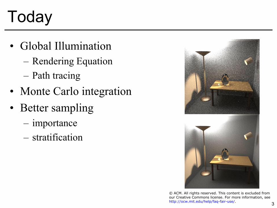
Today

• Lots of randomness!

Dunbar & Humphreys 2

3

Today

• Global Illumination – Rendering Equation – Path tracing

• Monte Carlo integration • Better sampling

– importance – stratification

3

© ACM. All rights reserved. This content is excluded fromour Creative Commons license. For more information, seehttp://ocw.mit.edu/help/faq-fair-use/.


Global Illumination • So far, we've seen only direct lighting (red here) • We also want indirect lighting

– Full integral of all directions (multiplied by BRDF) – In practice, send tons of random rays

4

Direct Illumination

5 Courtesy of Henrik Wann Jensen. Used with permission.

Global Illumination (with Indirect)


Global Illumination

• So far, we only used the BRDF for point lights – We just summed over all the point light sources

• BRDF also describes how indirect illumination reflects off surfaces – Turns summation into integral over hemisphere – As if every direction had a light source

7

Reflectance Equation, Visually

outgoing light to direction v

incident light from direction omega

the BRDF cosine term

v

Sum (integrate) over every

direction on the hemisphere,

modulate incident illumination by

BRDF

Lin

Lin

Lin

Lin

8

The Reflectance Equation

• Where does Lin come from?

x 9

The Reflectance Equation

• Where does Lin come from? – It is the light reflected towards x from the surface point in

direction l ==> must compute similar integral there! • Recursive!

x 10

• Where does Lin come from? – It is the light reflected towards x from the surface point in

direction l ==> must compute similar integral there! • Recursive!

– AND if x happens to be a light source, we add its contribution directly

The Rendering Equation

x 11

• The rendering equation describes the appearance of the scene, including direct and indirect illumination – An “integral equation”, the unknown solution function L

is both on the LHS and on the RHS inside the integral • Must either discretize or use Monte Carlo integration

– Originally described by Kajiya and Immel et al. in 1986 – More on 6.839

• Also, see book references towards the end


12

http://doi.acm.org/10.1145/15922.15902

http://doi.acm.org/10.1145/15922.15901


• Analytic solution is usually impossible • Lots of ways to solve it approximately • Monte Carlo techniques use random samples for

evaluating the integrals – We’ll look at some simple method in a bit...

• Finite element methods discretize the solution using basis functions (again!) – Radiosity, wavelets, precomputed radiance transfer, etc.

13

Questions?

14

How To Render Global Illumination?

Lehtinen et al. 2008


http://people.csail.mit.edu/jaakko/meshless/





Ray Casting

• Cast a ray from the eye through each pixel

16

Ray Tracing

• Cast a ray from the eye through each pixel • Trace secondary rays (shadow, reflection, refraction)

17

“Monte-Carlo Ray Tracing” • Cast a ray from the eye through each pixel • Cast random rays from the hit point to evaluate

hemispherical integral using random sampling

18

“Monte-Carlo Ray Tracing” • Cast a ray from the eye through each pixel • Cast random rays from the visible point • Recurse

19

“Monte-Carlo Ray Tracing” • Cast a ray from the eye through each pixel • Cast random rays from the visible point • Recurse

20

“Monte-Carlo Ray Tracing”

• Systematically sample light sources at each hit – Don’t just wait the rays will hit it by chance

21

Results H

enrik

Wan

n Je

nsen

22

Courtesy of Henrik Wann Jensen. Used with permission.

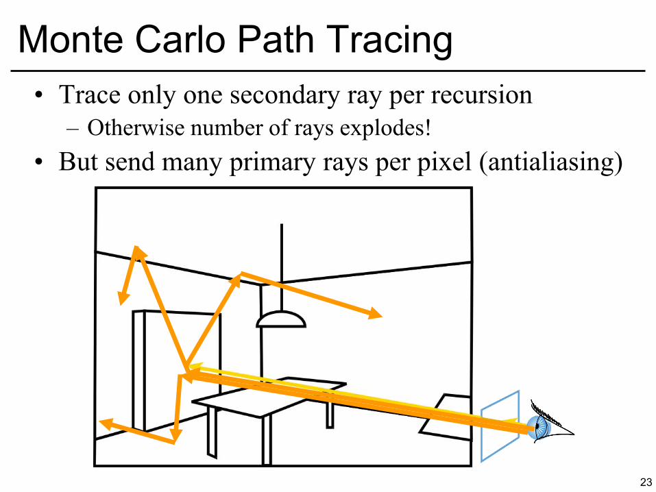
Monte Carlo Path Tracing • Trace only one secondary ray per recursion

– Otherwise number of rays explodes! • But send many primary rays per pixel (antialiasing)

23

Monte Carlo Path Tracing • Trace only one secondary ray per recursion

– Otherwise number of rays explodes! • But send many primary rays per pixel (antialiasing)

Again, trace shadow rays from each intersection

24

Monte Carlo Path Tracing • We shoot one path from the eye at a time

– Connect every surface point on the way to the light by a shadow ray

– We are randomly sampling the space of all possible light paths between the source and the camera

25

• 10 paths/pixel

Path Tracing Results H

enrik

Wan

n Je

nsen


Note: More noise. This is not a coincidence; the integrand has higher variance (the BRDFs are “spikier”).

• 10 paths/pixel

Path Tracing Results: Glossy Scene H

enrik

Wan

n Je

nsen


• 100 paths/pixel

Path Tracing Results: Glossy Scene H

enrik

Wan

n Je

nsen


Importance of Sampling the Light Without explicit light sampling

With explicit light sampling

1 path per pixel

4 paths per pixel

✔

✔ 29

Why Use Random Numbers?

• Fixed random sequence • We see the structure in the error

Hen

rik W

ann

Jens

en


Demo

• http://madebyevan.com/webgl-path-tracing/

31

Image removed due to copyright restrictions. Please see the above link for further details.

http://madebyevan.com/webgl-path-tracing/

For more demo/experimentation

• http://www.mitsuba-renderer.org/ • http://www.pbrt.org/ • http://www.luxrender.net/en_GB/index

32

http://www.mitsuba-renderer.org/

http://www.pbrt.org/

http://www.luxrender.net/en_GB/index

Questions?

• Vintage path tracing by Kajiya

33

© Jim Kajiya. All rights reserved. This content is excluded from our Creative Commonslicense. For more information, see http://ocw.mit.edu/help/faq-fair-use/.


Path Tracing is costly • Needs tons of rays per pixel!

34

Global Illumination (with Indirect)


Indirect Lighting is Mostly Smooth


Irradiance Caching

• Indirect illumination is smooth

37

Irradiance Caching

• Indirect illumination is smooth

38

Irradiance Caching

• Indirect illumination is smooth ==> Sample sparsely, interpolate nearby values

39

Irradiance Caching • Store the indirect illumination • Interpolate existing cached values • But do full calculation for direct lighting

40

Irradiance Caching

• Yellow dots: indirect diffuse sample points

The irradiance cache tries to adapt sampling density to expected frequency content of the indirect illumination (denser sampling near geometry)


Radiance by Greg Ward

• The inventor of irradiance caching • http://radsite.lbl.gov/radiance/

42

Image removed due to copyright restrictions. Please see above link for further details.

http://radsite.lbl.gov/radiance/

Questions?

Image: Pure 43

Image of Y chair designed by H.J. Wegner has been removed due to copyright restrictions. Please see http://tora_2097.cgsociety.org/portfolio/project-detail/786738/ for further details.

http://tora_2097.cgsociety.org/portfolio/project-detail/786738/

Photon Mapping

• Preprocess: cast rays from light sources, let them bounce around randomly in the scene

• Store “photons”

44

Photon Mapping

• Preprocess: cast rays from light sources • Store photons (position + light power + incoming direction)

45

The Photon Map

• Efficiently store photons for fast access • Use hierarchical spatial structure (kd-tree)

46

Photon Mapping - Rendering • Cast primary rays • For secondary rays

– reconstruct irradiance using adjacent stored photon – Take the k closest photons

• Combine with irradiance caching and a number of other techniques

Shooting one bounce of secondary rays and using the density approximation at those hit points is called final

gathering.

47

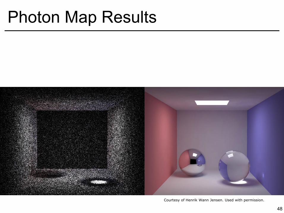
Photon Map Results

48

Courtesy of Henrik Wann Jensen. Used with permission.

• Many materials exhibit subsurface scattering – Light doesn’t just reflect off the surface – Light enters, scatters around, and exits at another point – Examples: Skin, marble, milk

More Global Illumination Coolness Im

ages

: Jen

sen

et a

l.


http://doi.acm.org/10.1145/383259.383319

More Subsurface Scattering

Photograph Rendering

Wey

rich

et a

l. 20

06

50

© ACM. All rights reserved. This content is excluded from our Creative Commonslicense. For more information, see http://ocw.mit.edu/help/faq-fair-use/.


http://doi.acm.org/10.1145/1141911.1141987

That Was Just the Beginning

• Tons and tons of other Monte Carlo techniques – Bidirectional Path Tracing

• Shoot random paths not just from camera but also light, connect the path vertices by shadow rays

– Metropolis Light Transport • And Finite Element Methods

– Use basis functions instead of random sampling – Radiosity (with hierarchies & wavelets) – Precomputed Radiance Transfer

• This would warrant a class of its own!

51

http://doi.acm.org/10.1145/127719.122740

http://doi.acm.org/10.1145/166117.166146

http://doi.acm.org/10.1145/566570.566612

What Else Can We Integrate? • Pixel: antialiasing • Light sources: Soft shadows • Lens: Depth of field • Time: Motion blur • BRDF: glossy reflection • (Hemisphere: indirect lighting)

52

© source unknown. All rights reserved. This content isexcluded from our Creative Commons license. For moreinformation, see http://ocw.mit.edu/help/faq-fair-use/.

© source unknown. All rights reserved.This content is excluded from our CreativeCommons license. For more information,see http://ocw.mit.edu/help/faq-fair-use/.

Courtesy of Henrik Wann Jensen.Used with permission.

© ACM. All rights reserved. This content isexcluded from our Creative Commonslicense. For more information, seehttp://ocw.mit.edu/help/faq-fair-use/.




Domains of Integration

• Pixel, lens (Euclidean 2D domain) – Antialiasing filters, depth of field

• Time (1D) – Motion blur

• Hemisphere – Indirect lighting

• Light source – Soft shadows

Famous motion blur image from Cook et al. 1984



http://doi.acm.org/10.1145/964965.808590

• Rendering glossy reflections • Random reflection rays around mirror direction

– 1 sample per pixel

Motivational Eye Candy

54

© source unknown. All rights reserved. This content is excluded from our CreativeCommons license. For more information, see http://ocw.mit.edu/help/faq-fair-use/.


• Rendering glossy reflections • Random reflection rays around mirror direction

– 256 samples per pixel

Motivational Eye Candy

55 © source unknown. All rights reserved. This content is excluded from our CreativeCommons license. For more information, see http://ocw.mit.edu/help/faq-fair-use/.


Error/noise Results in Variance • We use random rays

– Run the algorithm again get different image

• What is the noise/variance/standard deviation? – And what’s really going on anyway?

56 © source unknown. All rights reserved. This content is excluded from our CreativeCommons license. For more information, see http://ocw.mit.edu/help/faq-fair-use/.


Integration • Compute integral of arbitrary function

– e.g. integral over area light source, over hemisphere, etc.

• Continuous problem we need to discretize – Analytic integration never works because of visibility and other

nasty details

57

Integration

• You know trapezoid, Simpson’s rule, etc.

58

Monte Carlo Integration

• Monte Carlo integration: use random samples and compute average – We don’t keep track of spacing between samples – But we kind of hope it will be 1/N on average

59


• S is the integration domain – Vol(S) is the volume (measure) of S

• {xi} are independent uniform random points in S

60


• S is the integration domain – Vol(S) is the volume (measure) of S

• {xi} are independent uniform random points in S • The integral is the average of f times the volume of S • Variance is proportional to 1/N

– Avg. error is proportional 1/sqrt(N) – To halve error, need 4x samples

61

Monte Carlo Computation of

• Take a square • Take a random point (x,y) in the square • Test if it is inside the ¼ disc (x2+y2 < 1) • The probability is /4

x

y Integral of the function that is one inside the circle, zero outside

62

Monte Carlo Computation of

• The probability is /4 • Count the inside ratio n = # inside / total # trials • n * 4 • The error depends on the number or trials

Demo def piMC(n): success = 0 for i in range(n): x=random.random() y=random.random() if x*x+y*y<1: success = success+1 return 4.0*float(success)/float(n)

63

Why Not Use Simpson Integration?

• You’re right, Monte Carlo is not very efficient for computing

• When is it useful? – High dimensions: Convergence is independent of

dimension! – For d dimensions, Simpson requires Nd domains (!!!) – Similar explosion for other quadratures (Gaussian, etc.)

64

Advantages of MC Integration

• Few restrictions on the integrand – Doesn’t need to be continuous, smooth, ... – Only need to be able to evaluate at a point

• Extends to high-dimensional problems – Same convergence

• Conceptually straightforward • Efficient for solving at just a few points

65

Disadvantages of MC

• Noisy • Slow convergence • Good implementation is hard

– Debugging code – Debugging math – Choosing appropriate techniques

66

Questions?

• Images by Veach and Guibas, SIGGRAPH 95

Naïve sampling strategy Optimal sampling strategy



http://doi.acm.org/10.1145/218380.218498

Hmmh...

• Are uniform samples the best we can do?

68

Smarter Sampling

Sample a non-uniform probability Called “importance sampling” Intuitive justification: Sample more in places where there are

likely to be larger contributions to the integral

69

Example: Glossy Reflection

• Integral over hemisphere • BRDF times cosine times incoming light

Slide courtesy of Jason Lawrence

70

Image removed due to copyright restrictions – please see Jason Lawrence’s slide 9-12 in the talk slides on “Efficient BRDFImportance Sampling Using a Factored Representation,” available at http://www.cs.virginia.edu/~jdl/.

http://www.cs.virginia.edu/~jdl/

Sampling a BRDF Slide courtesy of Jason Lawrence

71




72




73



Importance Sampling Math

• Like before, but now {xi} are not uniform but drawn according to a probability distribution p

– Uniform case reduces to this with p(x) = const. • The problem is designing ps that are easy to sample

from and mimic the behavior of f

74

Monte Carlo Path Tracing

http://www.youtube.com/watch?v=mYMkAnm-PWw 75

Video removed due to copyright restrictions – please see the link below for further details.

http://www.youtube.com/watch?v=mYMkAnm-PWw

Questions?

Traditional importance function Better importance by Lawrence et al.

1200 Samples/Pixel



Stratified Sampling

• With uniform sampling, we can get unlucky – E.g. all samples clump in a corner – If we don’t know anything of the integrand,

we want a relatively uniform sampling • Not regular, though, because of aliasing!

• To prevent clumping, subdivide domain into non-overlapping regions i – Each region is called a stratum

• Take one random sample per i

77

Stratified Sampling Example

• When supersampling, instead of taking KxK regular sub-pixel samples, do random jittering within each KxK sub-pixel

78

Stratified Sampling Analysis

• Cheap and effective • But mostly for low-dimensional domains

– Again, subdivision of N-D needs Nd domains like trapezoid, Simpson’s, etc.!

• With very high dimensions, Monte Carlo is pretty much the only choice

79

Questions? • Image from the ARNOLD Renderer by Marcos Fajardo

80

Images removed due to copyright restrictions -- Please seehttp://www.3dluvr.com/marcosss/morearni/ for further details.

http://www.3dluvr.com/marcosss/morearni/

• 6.839! • Eric Veach’s PhD dissertation

http://graphics.stanford.edu/papers/veach_thesis/

• Physically Based Rendering by Matt Pharr, Greg Humphreys

For Further Information...

81

http://graphics.stanford.edu/papers/veach_thesis/

http://www.amazon.com/Physically-Based-Rendering-Implementation-Interactive/dp/012553180X

References

82

Images of the following book covers have been removed due to copyright restrictions:-Advanced Global Illumination by Philip Dutre, Philippe Bekaert, and Kavita Bala

-Realistic Ray Tracing by Peter Shirley and R. K. Morley

-Realistic Image Synthesis Using Photon Mapping by Henrik Wann JensenPlease check the books for further details.

That’s All for today

Image: Fournier and Reeves, SIGGRAPH 86 83

Image removed due to copyright restrictions -- please Fig. 13 in Fournier A. and W.T. Reeves. "A Simple Model of Ocean Waves."

SIGGRAPH '86 Proceedings of the 13th Annual Conference on Computer Graphics and Interactive Techniques; Pages 75-84.

MIT OpenCourseWarehttp://ocw.mit.edu

6.837 Computer Graphics Fall 2012

For information about citing these materials or our Terms of Use, visit: http://ocw.mit.edu/terms.

http://ocw.mit.edu

http://ocw.mit.edu/terms

Global Illumination and Monte Carlo - MIT OpenCourseWare · What Else Can We Integrate? • Pixel:...

Documents

Transcript of Global Illumination and Monte Carlo - MIT OpenCourseWare · What Else Can We Integrate? • Pixel:...