Global Existence for a Quasilinear Wave Equation Outside of Star-Shaped Domains

155

⁄0022-1236/02 $35.00

© 2002 Elsevier Science (USA)All rights reserved.

Journal of Functional Analysis 189, 155–226 (2002)doi:10.1006/jfan.2001.3844, available online at http://www.idealibrary.com on

Global Existence for a Quasilinear Wave EquationOutside of Star-Shaped Domains1

1 The authors were supported in part by the NSF.

Markus Keel

Department of Mathematics, University of Minnesota, Minneapolis, Minnesota 55455

Hart F. Smith

Department of Mathematics, University of Washington, Seattle, Washington 98195

and

Christopher D. Sogge

Department of Mathematics, The Johns Hopkins University, Baltimore, Maryland 21218

Communicated by Haim Brezis

Received February 15, 2001; accepted July 22, 2001

in memory of tom wolff

We prove global existence of small-amplitude solutions of quasilinear Dirichlet-wave equations outside of star-shaped obstacles in (3+1)-dimensions. We use avariation of the conformal method of Christodoulou. Since the image of the space-time obstacle is not static in the Einstein diamond, our results do not followsdirectly from local existence theory as did Christodoulou’s for the nonobstacle case.Instead, we develop weighted estimates that are adapted to the geometry. Usingthem and the energy-integral method we obtain solutions in the Einstein diamondminus the dime-dependent obstacle, which pull back to solutions in Minkowskispace minus and obstacle. © 2002 Elsevier Science (USA)

1. INTRODUCTION

The purpose of this paper is to establish global existence of small-ampli-tude solutions for certain quasilinear Dirichlet-wave equations outside of

smooth, compact star-shaped obstacles K … R3. Precisely, we shall con-sider smooth quasilinear systems of the form

“2t u − Du=F(u, du, d2u), (t, x) ¥ R+×R30K

u(t, · )|“K=0

u(0, · )=f, “tu(0, · )=g,

(1.1)

which satisfy the so-called null condition [15]. The global existence for suchequations in the absence of obstacles was established by Christodoulou [2]and Klainerman [11] using different techniques. We begin by describing ourassumptions in more detail.

We let a denote an N-tuple of functions, u=(u1, u2, ..., uN). We assumethat K is smooth and strictly star-shaped with respect to the origin. Bythis, we understand that in polar coordinates x=rw, (r, w) ¥ [0,.) × S2,we can write

K={x=rw : f(w) − r \ 0}, (1.2)

where f is a smooth positive function on S2. Thus,

0 ¥K, but 0 ¨ “K={x: r=f(w)}.

By quasilinearity, we mean that F(u, du, d2u) is linear in the secondderivatives of u. We shall also assume that the highest order nonlinearterms are diagonal, by which we mean that, if we denote “0=“t, then

FI(u, du, d2u)=GI(u, du)+ C0 [ j, k [ 3

cI, jk(u, du) “j “kuI, 1 [ I [ N. (1.3)

A key assumption is that the nonlinear terms satisfy the null condition.Recall that even in the obstacle-free case there can be blowup in finite timefor arbitrarily small data if this condition is not satisfied (see John [9]).

The first part of the null condition is that the nonlinear terms are free oflinear terms,

F(0, 0, 0)=0 and FŒ(0, 0, 0)=0. (1.4)

Additionally, we assume that the quadratic terms do not depend on u,which means that we can write

F(u, du, d2u)=Q(du, d2u)+R(u, du, d2u), (1.5)

where Q is a quadratic form and where the remainder term R vanishes tothird order at (u, du, d2u)=0; that is,

R(p, q, r)=O((p2+q2) r)+O((|p|+|q|)3). (1.6)

156 KEEL, SMITH, AND SOGGE

The null condition concerns the quadratic term Q. To describe it, wesplit Q into its semilinear and quasilinear parts:

Q(du, d2u)=s(du, du)+k(du, d2u).

Then in terms of the N components of u we can rewrite these terms as

sI(du, du)= C1 [ J, K [N

C0 [ j, k [ 3

sI, j, kJ, K “juJ“kuK

and

kI(du, d2u)=CN

j=1C

0 [ i, j, k [ 3kI, i, j, kJ “iuJ “j “kuI,

where the sI, j, kJ, K and kI, i, j, kJ are constants. The null condition can then bestated succinctly as requiring that, if 1 [ I, J, K [ N,

C0 [ j, k [ 3

sI, j, kJ, K tjtk=0, if t20=t21+t22+t23,

and, if 1 [ I, J [ N,

C0 [ i, j, k [ 3

kI, i, j, kJ titjtk=0, if t20=t21+t22+t23.

For further discussion, we refer the reader to Christodoulou [2, pp. 277–278].

As was shown in [2] and [11], this condition forces the semilinear termssI(du, du) to be linear combinations of the basic null forms

q0(duJ, duK)=“0uJ “0uK− C3

j=1“juJ “juK, (1.7)

and

qij(duJ, duK)=“iuJ “juK−“juJ “iuK, 0 [ i, j [ 3. (1.8)

The quasilinear term kI(du, d2u) in turn must be a linear combination ofterms of the form

q(duJ, d “juI), 1 [ J [ N, 0 [ j [ 3, (1.9)

where q is a basic null form as in (1.7) and (1.8), along with terms of theform

“juJ(“2t uI− DuI), 1 [ J [ N, 0 [ j [ 3. (1.10)

QUASILINEAR WAVE EQUATION 157

In addition to the null condition, we must assume that the Cauchy dataf, g satisfy certain compatibility conditions at the boundary. We leave thestatement of these conditions to Definition 9.2.

As in Christodoulou’s (2) results for the nonobstacle case, we shall notneed to assume that the data have compact support. Instead, we make theassumption that f and g belong to certain weighted Sobolev spaces. Tostate our assumptions precisely, we recall the weighted Sobolev spaces usedby Christodoulou [2], which are given by the norm

||f||Hm, j(R3)= C|a| [ m

1FR3

(1+|x|2) |a|+j |“axf(x)|2 dx21/2

.

The associated weighted Dirichlet–Sobolev spaces for m=1, 2... aredefined by

Hm, jD (R30K)={f ¥ Hm, j(R30K) : f|“K=0}, (1.11)

where Hm, j(R30K) is the space of restrictions of elements of Hm, j(R3).Hence,

||f||2Hm, jD = C|a| [ m

FR30K

(1+|x|2) |a|+j |“axf(x)|2 dx (1.12)

gives the natural norm on Hm, jD (R30K). We can now state our main result.

Theorem 1.1. Assume that K and F(u, du, d2u) are as above. Assumefurther that (f, g) ¥ C.(R30K) satisfies the compatibility conditions toinfinite order (see Definition 9.2). Then there exists e0 > 0, such that if

||f||H9, 8D (R30K)+||g||H8, 9D (R30K) < e0, (1.13)

then there is a unique solution u ¥ C.(R+×R30K) of (1.1). Furthermore,for all s > 0, there exists Cs <., such that

|u(t, x)| [ Cs(1+t)−1 (1+|t − |x| |)−1+s. (1.14)

We will actually establish existence of limited regularity solutions u fordata f ¥ H9, 8

D and g ¥ H8, 9D satisfying compatibility conditions of order 8;

see Theorem 7.1. The fact that u is smooth if f and g are smooth andsatisfy compatibility conditions of infinite order will follow by the localexistence theorems of Section 9.

It should be possible to relax the regularity assumptions in the smallnesscondition (1.13). In particular, our techniques should just require that||f||H4, 3D +||g||H3, 4D be small, which would be the analog of Christodoulou’sassumption in [2]. Additionally, the result should hold with s=0.


The authors [10] were able to show that if K is strictly convex then onehas global existence for the semilinear case for data f ¥ H2, 1

D and g ¥ H1, 2D .

The work was based on a variant of Christodoulou’s method whichinvolved weighted estimates, where, as in the present work, the weights onthe derivatives compensate for the degeneracy of the image of R+×“K ast Q +. under Penrose’s conformal compactification of Minkowski space.The proof depended on results of the last two authors [24] which extendedestimates of Klainerman and Machedon [15] to the setting of strictlyconvex obstacles. These results are not known in the setting of general star-shaped obstacles.

The special case of Theorem 1.1 in which one assumes spherical symme-try for u and K was obtained by Godin in [4]. His proof involved anadaptation of Christodoulou’s [2] method to this setting. If one drops theassumption of spherical symmetry, it does not appear that the arguments in[4] will apply in a straightforward way.

Also, results similar to those in Theorem 1.1 were announced in Datti[3], but there appears to be a gap in the argument which has not beenrepaired.

Previous work in higher dimensions applied Lorentz vector field tech-niques to the exterior problem. For general nonlinearities quadratic in du,global smooth solutions were shown by Shibata and Tsutsumi [20, 21] toexist for dimensions n \ 6. In Hayashi [5], global existence of smoothsolutions in the exterior of a sphere for n \ 4 is shown for a restricted classof quadratic nonlinearities.

Let us give an overview of our proof of Theorem 1.1. First of all, asin Christodoulou [2], we shall use the so-called conformal method (seealso [6]). Thus, we shall apply Penrose’s conformal compactification ofMinkowski space. Recall this is a map P: R×R3Q (−p, p) × S3, where theimage is the so-called Einstein diamond

E4={(T, X) ¥ (−p, p) × S3 : |T|+R < p} … E4=(−p, p) × S3.

Here R denotes the distance on S3 from the north pole

1=(1, 0, 0, 0)

measured in the standard metric. The Penrose map preserves the angularvariable, while if r is the radial variable and t the time variable inMinkowski space then under P the corresponding variables in E4 arerelated as follows

R=arctan(t+r) − arctan(t − r),

T=arctan(t+r)+arctan(t − r).(1.15)


Under this map the pushforward of the Minkowski metric dt2− dx2 isthe Lorentz metric g in E4 given by

dT2− g=W2g, (1.16)

where dT2− g is the standard Lorentz metric on R× S3 and where the con-formal factor W is given by the formula

W=cos T+cos R=2

(1+(t+r)2)1/2 (1+(t − r)2)1/2, (1.17)

with (T, R) and (t, r) being identified as above.Continuing, let

ig=“2T − Dg

be the D’Alembertian coming from the standard Laplace–Beltrami opera-tor Dg on S3. If we change our earlier notation a bit and let i denote theD’Alembertian on R1+3 or E4, depending on the context that arises fromthe standard Lorentz metric dt2− dx2, then a key fact for us is the way thatthe two D’Alembertians are related in E4:

ig+1=W−3i W, (1.18)

with the additive constant 1 arising because of the nonzero scalar curvatureof g. Equivalently,

iu=F Z (ig+1) v=G with u=Wv and G=W−3F. (1.19)

On account of this, if

Kg=P([0, +.) ×K) (1.20)

is the pushforward of our obstacle in Minkowski space, then the task ofshowing that we can find small-amplitude solutions of (1.1) is equivalent toshowing that we can find small-amplitude solutions of

(ig+1) v=G(v, dv, d2v), (T, X) ¥ E4+0Kg

v(T, X)=0, (T, X) ¥ “Kg

with E4+={(T, X) ¥ E4 : 0 [ T < p}, and u, v, F, and G related as above.Christodoulou [2] showed that the transformed nonlinear term G

extends to a nonlinear term with C. coefficients on the cylinder R× S3 ifand only if the null condition is satisfied. Indeed, the transformed quadra-tic terms coming from Q in (1.5) extend analytically to the cylinder if and


only if the null condition is verified (see [2, pp. 277–278]), while the trans-formed remainder term coming from R trivially extends smoothly becauseof (1.6) and (1.19). Because of this, as was argued in [2], the assertion thatthere are small-amplitude global solutions for (“2t − D) u=F(u, du, d2u)verifying the null condition in the boundaryless Minkowski case justfollows from a routine local existence theorem for R+× S3.

This simple approach breaks down for obstacle problems due to the factthat the transformed obstacle Kg given by (1.20) is a time-dependentobstacle which collapses to a point as T Q p. Indeed, it follows from (1.15)that there must be a uniform constant 1 < C <. so that for 0 [ T < p

C−1(p − T)2 [ dist(X, 1) [ C(p − T)2, if (T, X) ¥ “Kg, (1.21)

with 1 as above being the north pole on S3. Thus, if we let

P0=(p, 1), (1.22)

it follows that Kg collapses to P0 as T Q p.Following the approach in our earlier work [10], we shall surmount this

difficulty by modifying the usual existence arguments for the nonobstaclecase. In our approach, we shall need to obtain and apply estimates thatinvolve weighted derivatives because of the quadratic degeneracy of Kg at P0.

To state our main estimates we need to introduce some more notation.We let Xj, j=0, 1, 2, 3 be the coordinate functions on R4 and then let

“

“T, Xj

“

“Xk− Xk

“

“Xj, 0 [ j < k [ 3 (1.23)

be the spanning set of vector fields on E4, where we identify S3={X ¥ R4 : |X|=1}.

We arrange these vector fields as C={C0, ..., C6}. Our main estimateswill involve the weighted derivatives

Za=[(p − T)2 C]a=((p − T)2 C0)a0 · · · ((p − T)2 C6)a6. (1.24)

These turn out to be natural to use due to the fact that, near Kg, Zj pullsback via P to a vector field in Minkowski space that essentially has unitlength. As a side remark, this is not the case near the set where T+R=p,and this accounts for the importance of the null condition in three spatialdimensions.

To show that we can solve the transformed equation, and hence theoriginal (1.1), we need certain L2 estimates and pointwise estimates involv-ing Za. Special cases of the L2 estimates state that if v solves the Dirichlet-wave equation (ig+1) v=G, v|“Kg =0, then under appropriate conditionson the data and forcing terms we have


C|a| [ k

||ZavŒ(T, · )||2 [ Ck FT

0C|a| [ k

||ZaG(S, · )||2 dS

+Ck sup0 < S < T

(p − S)2 C|a| [ k−1

||ZaG(S, · )||2

+Ck C|a| [ k

||ZavŒ(0, · )||2, 0 < T < p, (1.25)

where, for a given T, the norms are taken over {(X: (T, X) ¥ E4+0Kg}. Thekey step in the proof of this will be to show that the bounds hold whenk=0:

||vŒ(T, · )||2 [ C ||vŒ(0, · )||2+C FT

0||G(S, · )||2 dS. (1.26)

Here, as throughout this paper, vŒ denotes the unweighted 4-gradient of v,or equivalently vŒ denotes the collection {Cjv, 0 [ j [ 6}.

To prove (1.26) we shall adapt Morawetz’s [18] proof of a related esti-mate in Minkowski space outside star-shaped obstacles. The proof of (1.26)is based on the fact that, when one applies standard arguments involvingthe energy-momentum tensor, the boundary integrals that arise haveintegrands with a favorable sign. Because of this, we can also obtain energyestimates for appropriate small variable coefficient perturbations of ig.The fact that the analog of (1.25) remains valid in this setting is necessaryto handle the nonlinear perturbations of the metric in (1.1). If X=Pg(“/“t) isthe pushforward of the Minkowski time derivative, then a key step in seeingthat (1.25) follows from (1.26) is that a variant of (1.26) holds when v isreplaced by Xv, since Xv also satisfies the Dirichlet boundary condition.

A special case of our pointwise estimate states that if (ig+1) v=G,v|Kg =0, then under appropriate assumptions on the data and forcing term,if p > 1 is fixed then for 0 < T < p we have uniform bounds

|v(T, X)| [ C sup0 [ S [ T

C|a| [ 1

(||ZaG(S, · )||2+(p − S)−2 ||ZaG(S, · )||p)

+C C|a| [ 1

||ZavŒ(0, · )||2. (1.27)

We shall also obtain analogous estimates for Zav. These estimates implythat the solution of the transformed version of (1.1) to E4+ satisfies

Zav(T, X)=O((p − T)−s) for s > 0. (1.28)

For technical reasons, we do not obtain uniform bounds s=0 due to thefact that (1.27) only holds for Lebesgue exponents p > 1.


In our earlier work [10] on the semilinear case, we showed only that thesolution of the transformed version of (1.1) satisfies (1.28) with s=1. Aswe shall see, the fact that we can now obtain bounds which blow up like(p − T)−s for some s < 1 plays a crucial role in our analysis. This is becausethe iterations we shall use in this paper would involve logarithmic terms ifs=1 and hence be useless.

We also remark that the proof of (1.28) is modeled after the recent proofby the last two authors [25] of global Strichartz estimates outside ofconvex obstacles.

2. THE CONFORMAL TRANSFORMATION ANDTHE TRANSFORMED EQUATION

In this section we provide further details about the conformal method. Inparticular, we recall formulas which relate derivatives in Minkowski spaceto derivatives in the Einstein diamond. We also go over estimates for thenonlinear terms of the pushforward via P of equations such as (1.1) whichsatisfy the null condition. As we stressed in the Introduction, it is importantfor our analysis that the nonlinear terms are small near the ‘‘tip’’ P0 ofthe Einstein diamond defined by (1.22). Finally, we show how the weightedDirichlet–Sobolev spaces Hm, j

D in (1.12) are related to the usual Dirichlet–Sobolev spaces on the 3-sphere minus an obstacle.

We start by reviewing the way that derivatives transform under Penrose’sconformal compactification of Minkowski space. For this it is convenientto use stereographic projection coordinates on S3. We note that the southpole stereographic projection coordinates U arise as the restriction of P−1

to the slice T=0:

U=P−10 (X)=

sin R1+cos R

w=tan 1R22 w. (2.1)

The coordinates V of the stereographic north pole projection are obtainedby applying the Kelvin transform to the south pole stereographic coordi-nate,

Vj=|U|−2 Uj. (2.2)

To compute the pushforwards of vector fields on E1+3 it is convenient touse the vector fields Cj defined by (1.23). We then have the following result(see [6]).


Proposition 2.1. The pushforwards of “t and “xj by P are given by

“t=11+1 − |U|2

1+|U|2cos T2 “T − sin TOU, “UP (2.3)

=11+|V|2− 1|V|2+1

cos T2 “T+sin TOV, “VP (2.4)

and

“xj=− 2Uj

1+|U|2sin T “T+

12

((1+|U|2) cos T+1 − |U|2) “Uj

+(1 − cos T) UjOU, “UP (2.5)

=− 2Vj

1+|V|2sin T “T+

12

((1+|V|2) cos T+|V|2− 1) “Vj

+(1+cos T) VjOV, “VP. (2.6)

The pushforwards via P−1 of the vector fields Cj defined by (1.23) are givenby

Xj “Xk − Xk “Xj=xj “xk − xk “xj , 1 [ j < k [ 3, (2.7)

X0 “Xk − Xk “X0=12 (1+t2− |x|2) “xk+xk(“t+Ox, “xP), 1 [ k [ 3, (2.8)

and

“T=12 (1+t2− |x|2) “t+tOx, “xP. (2.9)

Finally, if W=cos T+cos R, then

“tW= − W sin T1 − |U|2

1+|U|2=−W sin T cos R, (2.10)

“xjW= − W2 cos T1+|U|2

Uj. (2.11)

Note that the coefficients of “T and “U in (2.3) and (2.4) are O((p − T)2)if 0 [ T < p and R [ (p − T)/4. Similarly, if |x| [ t/4, then the coefficientsof “t and “x in (2.5) and (2.6) are O(t2+|x|2). Hence we have the followinguseful result.

Proposition 2.2. In the region where |x| [ t/4 we can write

“t=C a0k(T, X) Ck and “xj=C ajk(T, X) Ck,


where, if P0 is as in (1.22), we have

|Caajk | [ C dist((T, X), P0)2− |a|, |a| [ 2.

Also, if 0 [ T < p and R [ (p − T)/4, then

“T=b00(t, x) “t+C b0k(t, x) “xk ,

and

X0 “Xj − Xj “X0=b0j(t, x) “t+C bjk(t, x), “xj ,

where if “=(“t, “x1 , ..., “x3 ) we have

|“abjk(t, x)| [ C(1+|t|+|x|)2− |a|, |a| [ 2.

Using the above facts about the way that derivatives transform we shallbe able to see how the nonlinear term in (1.1) transforms.

We begin by examining how the basic null forms q0 and qij defined by(1.7) and (1.8) transform. Let q be such a null form in Minkowski space.Then if u is a function on E4, following (1.19), we shall let u denote thefunction in Minkowski space2 which is the pullback of Wu via P. Following

2 Here, as in the next several sections, we shall denote functions on Minkowski space with atilde, while corresponding functions coming from (1.19) on the Einstein or R× S3 will nothave a tilde.

(1.19) again we see that

Q(u(T, X), du(T, X); v(T, X), dv(T, X))=W−3q(du(t, x), dv(t, x)),

P(t, x)=(T, X)

is the null form transformed to E4, in the sense that the following specialcase of (1.1)

(“2t − D) u=q(du, du), (t, x) ¥ R+×R30K

u(t, x)|“K=0,

u(0, · )=f, “t u(0, · )=g,

transforms via P to the following equation in E40Kg

(ig+1) u=Q(u, du; u, du)

u(T, X)=0, (T, X) ¥ “Kg

u(0, · )=f, “Tu(0, · )=g,


if the data satisfy

f=Pg0 (Wf) and g=Pg

0 (W2g), (2.12)

and if Kg is as in (1.20).To proceed, we need the following result.

Lemma 2.3. Let q be any of the basic null forms defined by (1.7) or(1.8), and let Q be as above. Then Q extends to a bilinear function of(u, du; v, dv) on R× S3 with analytic coefficients. Moreover, if {Cj} aredefined by (1.23), we can write

Q=Cj, k

a jk(T, X) CjuCkv+v Cj

b j1(T, X) Cju+u Cj

b j2(T, X) Cjv+c(T, X) uv,(2.13)

such that

Caa jk(P0)=0, |a| [ 1, and b ji(P0)=0, (2.14)

where P0=(p, 1) is as in (1.22).

This result was used in the authors’ earlier work [10]. The proof has twosteps. The difficult step was carried out by Christodoulou [2], where it wasshown that one can write Q as in (2.13) with the coefficients being analytic.Given this step we observe from Proposition 2.2 that if we restrict thecoefficients to the region where R [ (p − T)/4, then the a jk must vanish tosecond order at P0, while the b ji must vanish there. By combining these twosteps we get (2.14).

Lemma 2.3 provides the result we need for the transformation of thesemilinear part s(du, du) of the nonlinear terms of our equation. We nowconsider the quasilinear part k(du, d2u). Recall that k(du, d2u) must be acombination of terms of the form (1.9) and (1.10). We first consider theterm (1.9). If 0 [ j [ 3 is fixed, then by Lemma 2.3 and Eqs. (2.10) and(2.11), we can write

W−3q(d “xj u(t, x), dv(t, x))

=o(u(T, X), du(T, X), d2u(T, X); v(T, X), dv(T, X)),

where o, initially defined on E4, extends to a bilinear function of (u, du, d2u;v, dv) on R× S3 with analytic coefficients. Moreover, we can write theextension of o in the form


Cj, k

c i, jk(T, X) C, X) CivCjCku

+Cj, k

c jk0 (T, X) vCjCku+Cj, k

a jk(T, X) CjvCku+v Cj

b j1(T, X) Cju

+u Cj

b j2(T, X) Cjv+c(T, X) uv,

where here the a jk and b ji satisfy (2.14), and moreover

Cac i, jk(P0)=0, |a| [ 3, and Cac jk0 (P0)=0, |a| [ 2.

Last to handle the quasilinear null form (1.10), we just use (1.19) andProposition 2.1 to conclude that a term of the form “xj v(“2t u − Du) alsotransforms into a term of the above form.

By these observations we have essentially proven the following.

Proposition 2.4. Let F(u, du, d2u) be as in Theorem 1.1 and set

F(u(T, X), du(T, X), d2u(T, X))

=W−3F(u(t, x), du(t, x), d2u(t, x)), (T, X)=P(t, x). (2.15)

Then F extends to a function of (u, du, d2u) on R× S3 which is C. in all itsvariables. Moreover, if for a given 1 [ I [ N we letFI be the Ith componentofF, then

FI=Cj, k

cI, jk(T, X; u, du) CjCkuI+GI(T, X; u, du), (2.16)

where in the region {(T, X): 0 [ T < p, R [ 2(p − T)} if a is fixed one hasthe uniform bounds

|ZacI, jk| [ C(p − T)4 C|c| [ |a|

|ZcuŒ|+C(p − T)3 C|c| [ |a|

|Zcu|

+C C|c1|+|c2| [ |a|

((p − T)2 |Zc1u|+(p − T)4 |Zc1uŒ|)

× ((p − T)2 |Zc2u|+(p − T)4 |Zc2uŒ|) (2.17)

and

|ZaG| [ C(p − T)2 C|c1|+|c2| [ |a|

|Zc1uŒ| |Zc2uŒ|+C C|c1|+|c2| [ |a|

(p − T) |Zc1uŒ| |Zc2u|

+C C|c1|+|c2| [ |a|

|Zc1u| |Zc2u|+C C|c1|+|c2|+|c3| [ |a|

|Zc1u| |Zc2u| |Zc3u|,(2.18)


assuming in both cases that

(p − T)2 C|c| [ 1+|a|/2

|Zcu| [ B, (2.19)

where B is a fixed constant. Here, as before, Za=((p − T)2 C)a.We also have the following bounds,

|GI(T, X; u, du) −GI(T, X; v, dv)|

[ C(|u|+|v|)((p − T) |uŒ− vŒ|+|u − v|)

+C(|uŒ|+|vŒ|)((p − T)2 |uŒ− vŒ|+(p − T) |u − v|), (2.20)

and

|cI, jk(T, X; u, du) − cI, jk(T, X; v, dv)| [ C((p − T)2 |uŒ− vŒ|+|u − v|), (2.21)

assuming that condition (2.19) holds with |a|=0.

If R(u, du, d2u) — 0 in (1.5), then these results follow from our earlierbounds for the transformed semilinear and quasilinear quadratic terms. Onthe other hand, since R(u, du, d2u) is linear and diagonal in the secondderivatives of u, and since it satisfies (1.6), it follows that if Q(du, d2u) — 0in (1.5) then the above bounds must hold if (2.19) holds. Indeed, we canwrite

RI(u, du, d2u)=O(|u|3+|du|3)+C rI, jk(u, du) “j “k u,

where rI, jk=O(|u|2+|“t, x u|2). The semilinear part of the remainder is con-trolled by the last term in (2.18), since its transformed version must beO(|u|3)+O((p − T)6; |Cju|3) on the region in the diamond R [ 2(p − T).Likewise, the quasilinear part of the remainder is controlled by the lastterm in (2.17), since it transforms to ; rI, jk(u, du) CjCku where

rI, jk(u, du)=O 1 (p − T)4 |u|2+(p − T)8 C |Cju|22 if R [ 2(p − T).

We now recall standard facts about how the Sobolev spaces in (1.11)transform under P0. Recall that the inverse of P0 is the south polestereographic projection map, and so P0(K) … S3 is star-shaped withrespect to the north pole and has smooth boundary. For m=1, 2, ... wethen let

HmD(S30P0(K))={f ¥ Hm(S30P0(K)) : f|“P0(K)=0},

with Hm(S30P0(K)) being the Sobolev space of restrictions of elements ofHm(S3).


If then Pg0 f denotes the pullback of the function f on S30P0(K) via P0,

and we relate f to f via

f=WPg0 f,

then the map f Q f is continuous from Hm, m−11(R30K) to Hm(S30P0(K)).That is, for fixed m there is a constant Cm so that

||f||Hm(S30P0(K)) [ Cm ||WPg0 f||Hm, m−1(R30K)=Cm ||f||Hm, m−1(R30K).

Thus, if u=WP*u, then

||u(0, · )||Hm(S30P0(K))+||“Tu(0, · )||Hm−1(S30P0(K))

[ Cm ||u(0, · )||Hm, m−1(R30K)+Cm ||“t u(0, · )||Hm−1, m(R30K), (2.22)

since the pushforward of “t is W “T if t=0 and since W=2/(1+|x|2) ift=0.

We close this section by presenting some of the notation that we shall usein the rest of the paper. First of all we shall let

Y=([0, p) × S3)0Kg, (2.23)

where Kg=P(K). Thus, Y is the image of Minkowski space minus theobstacle. Also, for each fixed 0 [ T < p, we let

YT={X ¥ S3 : (T, X) ¥ Y} (2.24)

be the T cross section of Y.Next, by dilating the Minkowski variables if necessary, we will assume

that

“K … {x ¥ R3 : |x| < 1/4}. (2.25)

If we then let

r=r(T, X)=sin(R)

cos T+cos R

be the spatial radial component of P−1(T, X), it follows that

“Y …B1/4, (2.26)

where we define

Br={(T, X) ¥ [0, p) × S3 : r(T, X) < r}. (2.27)


Thus, Br is the pushforward of the cylinder R+× {x: |x| < r} via P. Equa-tion (1.15) implies that if r0 > 0 is fixed, and if 0 [ r [ r0, then there is auniform constant C=C(r0) so that

C−1r(p − T)2 [ R [ Cr(p − T)2, if (T, X) ¥ “Br. (2.28)

As before, R denotes the north pole distance on S3 measured with respectto the standard metric. If 0 [ T < p, we shall let BT

r denote the T crosssection of Br,

BTr ={X ¥ S3 : (T, X) ¥BR}. (2.29)

3. FIRST ORDER ESTIMATES

Let ig=“2T − Dg be the wave operator on R× S3, where gjk(X) dXj dXk

is the standard metric on S3. In this section we shall prove energy estimatesfor certain perturbations of ig in Y, where as in (2.23) we let Y denote theimage of Minkowski space minus the strictly star-shaped obstacle.

Before proving energy estimates for perturbations of ig, we first handleig itself since the arguments in this case are simpler and serve as a modelfor the more technical case involving perturbations. The argument that weshall use is similar to that of Morawetz [18] (see also [17, pp. 261–264])for a related energy-decay estimate in Minkowski space minus a star-shaped obstacle. In particular, we shall see that when one goes through thestandard proof of energy estimates the (variable) boundary contributes aterm with the ‘‘correct’’ sign if K is strictly star-shaped with respect to theorigin. When we handle perturbations of ig there will be additionalboundary terms coming from the perturbation, but these will be absorbedby the Morawetz term under smallness assumptions for the perturbation.

We introduce the energy momentum 4-vector e associated to a functionu(T, X) on R× S3, defined by

e0=|“Tu|2+||grad u||2

ej= − 2(“Tu) grad u, 1 [ j [ 3,

where grad and || · || are associated to the metric g. In local coordinates,

(grad u)j= C3

k=1g jk(X) “ku(T, X),

||grad u||2= C3

k=1g jk(X) “ju(T, X) “ku(T, X).


For convenience in future use, we will use the abbreviation

|uŒ(T, X)|2 — e0(T, X).

Theorem 3.1. Suppose that K … R3 is strictly star-shaped with respectto the origin. Suppose also that u ¥ C2 and u(T, X)=0 if (T, X) ¥ “Y, and let

F=ig u.

Then for 0 < T < p

||uŒ(T, · )||L2(YT) [ ||uŒ(0, · )||L2(Y0)+FT

0||F(S, · )||L2(YS) dS. (3.1)

Here the L2-norms are taken with respect to the volume element arisingfrom the metric g.

We prove Theorem 3.1 by applying the divergence theorem to the vectorfield e on Y 5 [0, T] × S3. Precisely, we consider R× S3 as a Riemannianmanifold with metric dT2+g. In local coordinates, the divergence of e thenequals

“Te0+1

`|g|C3

j=1“j(`|g| ej)=2(“Tu) F.

The divergence theorem yields:

FYT

e0(T, · ) dX −FY0

e0(0, · ) dX+F“Y 5 [0, T]×S3

On, eP ds

=2 FY 5 [0, T]×S3

(“Tu) F dT dX.

Here, n denotes the outer unit normal to “Y in the metric dT2+g. We write

n(nT, nX), (nT)2+||nX ||2=1. (3.2)

The vector (1, nTnX/||nX ||2) is tangent to “Y, and by the Dirichlet conditionsfor u we thus have

“Tu=nT ||nX ||−2 “nXu for (T, X) ¥ “Y. (3.3)

Combining (3.2) and (3.3) shows that

(“nu)2=(nT “Tu+“nXu)2=||nX ||−4 (“nXu)2. (3.4)


By Dirichlet conditions on u,

e0(T, X)=(“nu)2, for (T, X) ¥ “Y.

Combining (3.2), (3.3), and (3.4) yields

On, eP=nT(“nu)2− 2(“Tu)(“nXu)=−nT(||nX ||2− n2T)(“nu)2. (3.5)

Consequently,

FYT

e0(T, · ) dX −FY0

e0(0, · ) dX −F“Y 5 [0, T]×S3

nT(||nX ||2− n2T) e0(T, X) ds

=2 FY 5 [0, T]×S3

(“Tu) F dT dX.

The important observation now is that nT is strictly negative. Indeed,working in polar coordinates about the north pole, by (1.2) we can write

“Kg={(T, F(T, w)): 0 [ T < p},

with F smooth. The crucial fact is that

“TF < 0, 0 < T < p. (3.6)

Indeed,

“TF=−4tf(r, w)/[(t+f(r, w))2+(t − f(r, w))2],

and so

“TF [ − c min{(p − T), T}, 0 [ T < p, (3.7)

for some fixed constant c > 0. These facts follow from our strict star-shaped hypothesis (1.2) and an elementary calculation.

From Eq. (3.7) and the fact that “Y is timelike, there is a uniform con-stant c > 0 so that

− nT(||nX ||2− n2T) \ c min{(p − T), T}, 0 [ T < p. (3.8)

An application of the Gronwall inequality completes the proof of thetheorem.

3.1. Energy Estimates for Perturbed Operators

In this section we work with a Lorentzian metric h which we shallassume to be a small perturbation of the standard Lorentz metric g defined by

g=dT2− g.


We letih denote the associated D’Alembertian, which in local coordinatestakes the form

ih u=|h|−1/2 C3

j, k=0“j(h jk |h|1/2 “ku), (3.9)

where (h jk)=(hjk)−1.We will assume that h is uniformly close to the standard metric,

|h(V, W) − g(V, W)| [ d, (3.10)

for all pairs of vectors V, W of norm one in the metric dT2+g. We willtake d sufficiently small (to be determined). We shall also assume that wehave the following bounds for the covariant derivatives of h − g withrespect to dT2+g,

||N(h − g)||L1TL.X [ C0. (3.11)

It will be convenient to use local coordinates in our calculations; we thuscover the sphere with two compact coordinate patches using north poleand south pole projective coordinates. We then write

h jk=g jk+c jk.

Expressed in these coordinate systems, our conditions are equivalent (up toconstants) to the following

C3

j, k=0||c jk(T, X)||L.T, X [ d,

C3

i, j, k=0||“ic jk(T, X)||L1TL.X [ C0. (3.12)

We then have the following

Theorem 3.2. Assume h is as above and let u ¥ C2 satisfy

ihu(T, X)=F(T, X), (T, X) ¥ Y

u(T, X)=0, (T, X) ¥ “Y.

Then if (3.10) holds for d > 0 sufficiently small, and if (3.11) holds, then

||uŒ(T, · )||L2(YT) [ C ||uŒ(0, · )||L2(Y0)+C FT

0||F(S, · )||L2(YS) dS, 0 < T < p,

(3.13)

for a uniform constant C (depending on C0).


To proceed, we introduce the energy-momentum vector

e=2(“Tu) gradh u −Ogradh u, gradh uP “T,

where gradh and O · , ·Ph denote the Lorentz gradient and inner product forh. In local coordinates,

e0=2(“Tu) C3

k=0h0k(T, X) “ku(T, X) − C

3

j, k=0h jk(T, X) “ju(T, X) “ku(T, X),

ej=2(“Tu) C3

k=0h jk(T, X) “ku(T, X), j=1, 2, 3.

We now apply the divergence theorem on Y 5 [0, T] × S3 using thedivergence (“T, div) associated to the standard Riemannian metric dT2+g.We first claim that

“T e0+div eX=2(“Tu)ihu+R(uŒ, uŒ),

where R( · , · ) is a quadratic form whose coefficients (in any orthonormalframe) belong to L1TL.X with norm bounded by some fixed multiple of C0.

To see this, we work in local coordinates. There, we may write

div eX=1

`|g|C3

j=1“j(`|g| ej)=C

3

j=1“j ej+C

3

j=1rj ej,

where the rj are uniformly bounded functions.Next, a simple calculation shows that

C3

j=0“j ej=2(“Tu) C

3

j, k=0“j(h jk “ku)+ C

3

j, k=0rjk “ju “ku,

where the coefficients rjk(T, X) involve first derivatives of the h jk and hencebelong to L1TL.X . The last expression may be written in the form

2(“Tu)ihu+R(uŒ, uŒ).

Next, we claim that

|On, e − eP| [ C d |nT | |uŒ|2.


(The inner product is with respect to dT2+g.) To see this, we write

On, e − eP=−nT 1 C3

j, k=0c jk “ju “ku2+2nT(“Tu) C

3

k=0c0k “ku

+2(“Tu) C3

i, j=1C3

k=0gijc jk “ku.

The first two terms clearly have the desired bounds; to handle the last, weuse (3.3).

It follows from (3.5) and (3.8) that for d sufficiently small, the boundaryterm On, eP is positive, and by the divergence theorem we have

FYT

e0(T, X) dX [ FY0

e0(0, X) dX+2 FY 5 [0, T]×S3

(“Tu) F dT dX

+FY 5 [0, T]×S3

R(uŒ, uŒ) dT dX.

The proof of the theorem now follows from the Gronwall lemma by notingthat, for d small, we have

C−1 |uŒ(T, X)|2 [ e0(T, X) [ C |uŒ(T, X)|2.

In Section 5 we shall use the fact that (3.13) holds for equations of the form

1ig+ C6

j, k=0c jkCjCk+12 u=F,

provided that

C6

j, k=0||c jk(T, X)||L.T, X [ d, (3.14)

C6

i, j, k=0||Cic jk(T, X)||L1TL.X [ C0. (3.15)

To see this, we note that there is a unique metric h such that the operator

ih −ig − C6

j, k=0c jkCjCk

is of first order. Furthermore the metric h satisfies the conditions (3.10)and (3.11) (with possibly different constants). We now just observe thatthe proof of Theorem 3.2 goes through if F is modified by first orderderivatives in u.


4. SOBOLEV ESTIMATES

For our applications in later sections, in addition to controlling the L2

norm of uŒ(T, · ), we also need to control the L6 norm of u(T, · ). For thiswe will make use of the following elementary result.

Lemma 4.1. Suppose that u ¥ C1 vanishes on “Y. Then there is a uniformconstant C so that for 0 [ T < p

||u(T, · )||L6(YT) [ C ||uŒ(T, · )||L2(YT)+C ||u(T, · )||L2(YT). (4.1)

The lemma follows from the Sobolev embedding H1+ L6 for the sphere

S3 by noting that the extension of u(T, · ) to the entire sphere, obtained bysetting it equal to 0 on the complement of YT, belongs to H1(S3) with normcontrolled by the right hand side of (4.1).

Using the lemma we can strengthen (3.13) somewhat.

Corollary 4.2. Let u be as in Theorem 3.2. Then

||uŒ(T, · )||L2(YT)+||u(T, · )||L6(YT)

[ C ||uŒ(0, · )||L2(Y0)+C FT

0||F(S, · )||L2(YS) dS, 0 < T < p. (4.2)

This follows from (3.13) and Lemma 4.1 above by noting that, since usatisfies Dirichlet conditions on “Y, we can bound

||u(T, · )||L2(YT) [ FT

0||uŒ(S, · )||L2(YS) dS+||u(0, · )||L2(Y0)

[ sup0 [ S [ T

||uŒ(S, · )||L2(YS)+C ||uŒ(0, · )||L2(Y0).

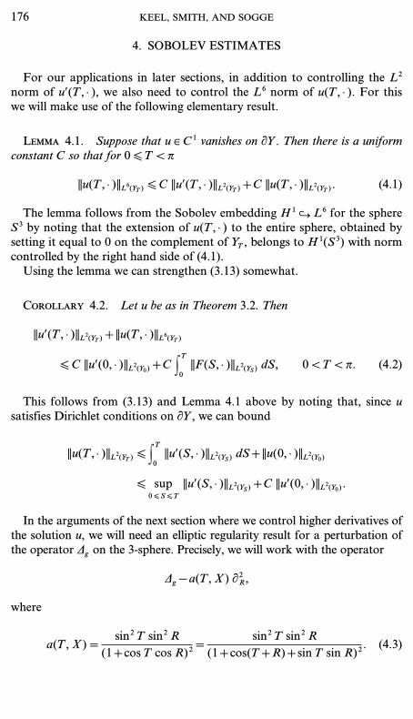
In the arguments of the next section where we control higher derivatives ofthe solution u, we will need an elliptic regularity result for a perturbation ofthe operator Dg on the 3-sphere. Precisely, we will work with the operator

Dg − a(T, X) “2R,

where

a(T, X)=sin2 T sin2 R

(1+cos T cos R)2=

sin2 T sin2 R(1+cos(T+R)+sin T sin R)2

. (4.3)


We use the fact that

a(T, X)=sin2(p − T) sin2 R

(1 − cos(p − T) cos R)2[ 1 2d

1+d222

if sin R=d sin(p−T), for d [ 1. Consequently, Dg−a(t, X) “2R is uniformlyelliptic on the set R < d(p − T) if d < 1. Also, from the fact that

1 − cos(p − T) cos R % 12 (p − T)2+1

2 R2,

for (T, R) near (p, 0), it is easy to see that

|Caa(T, X)| [ Ca[(p − T)2+R2]−|a|/2. (4.4)

Our estimate will involve the weighted derivatives Z=(p − T)2 C as in(1.24); we let

{ZX}={Zjk: 1 [ j < k [ 6}

be the set of weighted derivatives that do not involve “T and similarly define CX.

Proposition 4.3. Let k=0, 1, 2, ... . Then there is a constant C=C(k),independent of T, so that whenever h ¥ C.(Y) vanishes on “Y, then for0 [ T < p,

C|a| [ k+1

(||ZaXCXh(T, · )||L2(R < (p−T)/2)+||Za

Xh||L6(R < (p−T)/2))

[ C(p − T)2 C|a| [ k

||ZaX(Dg − a(T, X) “2R) h(T, · )||L2(R < p−T)

+C C|a| [ k

||ZaXh(T, · )||L6(R < p−T). (4.5)

We first show that the estimate holds if the norms on the left hand sideare taken over a set of the form R [ C0(p − T)2. To do this, we work insouth pole stereographic coordinates U on S3, which map the north pole tothe origin, and dilate in these variables by (p − T)2. After dilation, theboundary “YT is mapped to a surface MT … R3 contained in the setc [ R [ c−1, where c > 0 is independent of T, such that there are uniformbounds on the surface MT independent of T.

We next write Dg−a(T, X) “2R as LT(U, DU) in the stereographic coordi-nates. Then the operator PT=LT((p−T)2 U, “U) is seen to be a uniformlyelliptic operator on the image of the set R < d(p−T) for any d < 1, andfurthermore there are uniform bounds on the derivatives of the coefficients ofPT which are independent of 0 < T < p. In fact, this statement is true forLT((p−T) U, “U)), which follows from (4.4), together with the fact thata(T, X) vanishes quadratically at R=0 and the fact that “R is mapped understereographic coordinates to a smooth multiple of the radial vector field.


Because Z scales to a unit vector field under this dilation, the desired esti-mate is a result of the following estimate in the scaled coordinates, for func-tions f ¥ C.(Mext

T ) which vanish on MT,

C|a|[ k+1

(||“a(Nf)||L2(r [C0)+||“af||L6(r [C0))

[ C C|a|[ k

(||“a(PTf)||L6(r [ 2C0)+||“af||L6(r [ 2C0)),

and this estimate holds by standard elliptic regularity theory.We remark that this proof in fact shows that, to control the left hand side

of (4.5) over the set R < C0(p−T)2, it suffices to take the norms on the righthand side over the set R [ 2C0(p−T)2, a fact we will use in the proof ofProposition 6.2.

Now let f be a cutoff to the set R \ c(p−T)2, where c is chosen so thatf=0 on “Y. From the fact that ||Za NXf(T, · )||L3 [ C, and the estimates (4.4),it follows that

(p−T)2 C|a|[ k

||ZaX(Dg−a(T, X) “2R)(fh)(T, · )||L2(R [ p−T)

[ C(p−T)2 C|a|[ k

||ZaX(Dg−a(T, X) “2R) h(T, · )||L2(R < p−T)

+C C|a|[ k+1

||ZaXh(T, · )||L6(R < c(p−T)2).

By the preceding steps the last term is controlled by the right hand side of(4.5); consequently we are reduced to the case of establishing (4.5) in theabsence of a boundary.

To see that (4.5) holds in the absence of a boundary, we again work insouth pole stereographic coordinates, and now dilate by (p−T), so that theset R [ (p−T)/2 is mapped to a ball of radius close to 1/2. We now use thefact that PT=LT((p−T) U, “U) is uniformly elliptic on the region of interest,with smooth coefficients that have uniform bounds on 0 < T < p.

Next, by an induction argument we may consider just the terms on the lefthand side of (4.5) where |a|=k+1. Then, after scaling, we are led to theestimate

(p−T)k C|a|=k+1

(||“a(Nf)||L2(r [ 12 )+||“af||L6(r [ 12 ))

[ C C|a|[ k

(p−T) |a| (||“a(PTf)||L2(r [ 1)+(p−T)−1 ||“af||L6(r [ 1)).


Since the powers of (p−T) on the right are less than or equal to k, and(p−T) is bounded above, this estimate follows as before by elliptic regularitytheory.

5. HIGHER ORDER ESTIMATES

In this section, we establish a priori estimates on higher order weightedderivatives of the solution u, in terms of weighted derivatives of the coefficientscjk. For convenience, we assume that cjk and u belong to C.(Y), where werecall that Y=([0, p)×S3)0Kg.

We shall also assume that the cjk satisfy the hypotheses (3.14) and (3.15) sothat by Theorem 3.2 we have control of the L2-norm of uŒ.

Theorem 5.1. Suppose that cjk, u ¥ C.(Y), and that u(T, X)=0 if(T, X) ¥ “Y. Suppose that the cjk satisfy (3.14) and (3.15), where d > 0 in(3.14) is small enough so that (3.13) holds. Let

F=1ig+C cjkCjCk+12 u.

Then, given N=0, 1, 2, ..., there is a constant C depending only on N, d, andC0, so that for 0 [ T < p,

C|a|[N

(||ZauŒ(T, · )||2+||Zau(T, · )||6)

[ C C|a|[N

(||ZauŒ(0, · )||2+FT

0||ZaF(S, · )||2 dS)

+C sup0[ S[ T

(p−S)2 C|a|[N−1

||ZaF(S, · )||2

+C FT

0(p−S)−2C

j, kC

|a1|+|a2|[N+1|a1|, |a2|[N

(||(Za1cjk) Za2uŒ(S, · )||2

+||(Za1cjk) Za2u(S, · )||6) dS

+C sup0[ S[ T

Cj, k

C|a1|+|a2|[N|a1|[N−1

||(Za1cjk) Za2uŒ(S, · )||2. (5.1)

Remark. Before proving Theorem 5.1, we point out that if we fix N andassume that d > 0 is small enough so that C ;3

j, k=0 ||cjk||. < 1/2 then we canstrengthen (5.1) somewhat. Specifically, the part of the last summand in theright side of (5.1) where a1=0 and |a2|=N can be absorbed in the left side of(5.1). As a result, under this additional smallness assumption, we have


C|a| [N

(||ZauŒ(T, · )||2+||Zau(T, · )||6)

[ C C|a| [N

1 ||ZauŒ(0, · )||2+FT

0||ZaF(S, · )||2 dS2

+C sup0 [ S [ T

(p − S)2 C|a| [N−1

||ZaF(S, · )||2

+C FT

0(p − S)−2 C

j, kC

|a1|+|a2| [N+1|a1|, |a2| [N

(||(Za1c jk) Za2uŒ(S, · )||2

+||(Za1c jk) Za2u(S, · )||6) dS

+C sup0 [ S [ T

Cj, k

C|a1|+|a2| [N|a1|, |a2| [N−1

||(Za1c jk) Za2uŒ(S, · )||2.

We will establish Theorem 5.1 by induction. The inequality holds withN=0, by Theorem 3.2 and the remark at the end of Section 3. For N=0only the first two terms on the right are needed. We thus make the follow-ing

Induction hypothesis. Inequality (5.1) is valid if N is replaced by N − 1.

We then show that this implies (5.1) for N=N. To do this, we write thenorm on the left hand side of (5.1) as a sum of two terms, by separatelyconsidering the regions R < (p − T)/2 and R > (p − T)/2. We begin byconsidering R < (p − T)/2. To estimate this term, we will make use of thevector field X on Y obtained by pushing forward the Minkowski timederivative via the Penrose compactification,

X=Pg(“t).

We note that X is tangent to “Y, so that if u vanishes on “Y then so doesX; that is,

Xu(T, X)=0 if (T, X) ¥ “Y. (5.2)

We use the following formulae involving X:

Lemma 5.2. As above, let R denote the polar distance from the north polein S3. Then

X=(1+cos T cos R) “T − sin T sin R “R

=(1+cos(T+R)+sin T sin R) “T − sin T sin R “R. (5.3)


Moreover,

[ig, X]=−2 cos R sin Tig+2 cos R cos T “T+2 sin T sin R “R. (5.4)

The proof of this lemma is a straightforward calculation and will bepostponed until the end of this section.

If we let L=ig+; c jkCjCk+1 then (5.4) yields

LXu=XF − 2 cos R sin T 1F −Cj, k

c jkCjCku − u2

+2 cos R cos T “Tu+2 sin T sin R “Ru+Cj, k

[c jkCjCk, X] u. (5.5)

Now let f be a cutoff function such that f(T, X)=1 for R [ 2(p − T),and f(T, X)=0 for R \ 3(−p − T), and

Zaf(T, X) [ Ca. (5.6)

Let w solve the equation

Lw=f 1XF − 2 cos R sin T 1F −Cj, k

c jkCjCku − u2

+2 cos R cos T “Tu+2 sin T sin R “Ru+Cj, k

[c jkCjCk, X] u2 . (5.7)

Then, by finite propagation velocity, w=Xu for R [ (p − T). We will showthat if one takes the right hand side of (5.1) with N replaced by N − 1, andF replaced by the right hand side of (5.7), then the result is bounded by theright hand side of (5.1) with N=N. The induction hypothesis, using thefact that w=0 on “Y as a result of (5.2), will then show that the followingquantity is bounded by the right hand side of (5.1),

C|a| [N−1

||Za(Xu)Œ (T, · )||L2(R < (p−T))+||ZaXu(T, · )||L6(R < (p−T)).

Since (Xu)Œ=XuŒ+O(uŒ), we conclude that

C|a| [N−1

(||ZaXuŒ(T, · )||L2(R < (p−T))+||ZaXu(T, · )||L6(R < (p−T))) (5.8)

is also bounded by the right hand side of (5.1).To bound the right hand side of (5.1) with N replaced by N − 1 and F

replaced by the right hand side of (5.7), we first use (5.6) to note that itsuffices to bound the same quantity with F replaced by the right hand sideof (5.5), but with the norms taken over the set R [ 3(p − T).


Next, we notice that for R [ 3(p − T), one can write X as a combinationof the vector fields {Z}, with coefficients that satisfy the same estimates(4.4) as a(T, X). Based on this, one can see that

Cj, k

C|a| [N−1

(||Za[c jkCjCk, X] u||L2(R < 3(p−T))+||Za(c jkCjCku)||L2(R < 3(p−T)))

[ C(p − T)−2 Cj, k

C|a1|+|a2| [N+1|a1|, |a2| [N

||(Za1c jk) Za2uŒ(T, · )||2. (5.9)

Similarly,

C|a| [N−1

||ZaXF||L2(R < 3(p−T))+||ZaF||L2(R < 3(p−T)) [ C C|a| [N

||ZaF||2.

These terms are thus bounded by the right hand side of (5.1).To handle the remaining terms, which involve uŒ and u, we note that

C|a| [N−1

||Za(cos R cos T “Tu+sin T sin R “Ru)||2 [ C C|a| [N−1

||ZauŒ||2,

while

C|a| [N−1

||Za(cos R sin Tu)||2 [ C C|a| [N−1

||Zau||6.

By the induction hypothesis, the norms on the right hand side of these twoequations are in fact bounded by the right hand side of (5.1) with Nreplaced by N − 1, and thus with N=N.

Thus, we have shown that the quantity in (5.8) is bounded by the righthand side of (5.1). To proceed, we use (5.3) to write

(1+cos T cos R)(“2Tu − a(T, X) “2Ru)=X “Tu −sin T sin R

1+cos T cos RX “Ru,

where a(T, X) is as in (4.3). Since R \ c(p − T)2 on YT, we may write“Ru=b · uŒ where |Zab| [ Ca. Consequently, we may bound

C|a| [N−1

|Za((1+cos T cos R)(“2Tu−a(T, X) “2Ru))| [ C C|a| [N−1

|ZaXuŒ|+|ZauŒ|.

The L2 norm of the right hand side over R < (p − T) is bounded by thequantity (5.8), and consequently the following quantity is bounded by theright hand side of (5.1),

C|a| [N−1

||Za((1+cos T cos R)(“2Tu(T, · ) − a(T, X) “2Ru(T, · )))||L2(R < (p−T)).


We next write

Dgu − a(T, X) “2Ru=“2Tu − a(T, X) “2Ru+Cj, k

c jkCjCku+u − F.

Note that 1+cos R cos T % (p − T)2 for R < 3(p − T). Therefore

Cj, k

C|a| [N−1

|Za(1+cos T cos R) c jkCjCku(T, · )|

[ C Cj, k

C|a1|+|a2| [N|a1| [N−1

|(Za1c jk) Za2uŒ(T, · )|.

Based on this and the induction hypothesis we deduce that the followingquantity is bounded by the right side of (5.1)

C|a| [N−1

||Za((1+cos T cos R)(Dgu(T, · ) − a(T, X) “2Ru(T, · )))||L2(R < (p−T)),

and thus by Proposition 4.3 so is the following quantity

C|a| [N

||ZaXCXu||L2(R [ (p−T)/2)+||Za

Xu||L6(R [ (p−T)/2).

We write

X=(1+cos T cos R)(“T − b · CX).

Again from the fact that (1+cos T cos R) % (p − T)2 and the fact that (5.8)is bounded, the following quantity is bounded by the right hand side of(5.1),

C|a| [N

(p − T)2 |a| (||Ca(“T − b · CX) u||L2(R [ (p−T)/2)+||CaXCXu||L2(R [ (p−T)/2))

+ C|a| [N−1

(p − T)2 |a| (||Ca(“T − b · CX) u||L6(R [ (p−T)/2)

+||CaXCXu||L6(R [ (p−T)/2)).

A simple induction in the number of T derivatives shows that this in turnbounds the following quantity,

C|a| [N

(p − T)2 |a| (||CaCu||L2(R [ (p−T)/2)+||Cau||L6(R [ (p−T)/2)),


which is comparable to

C|a| [N

(||ZauŒ(T, · )||L2(R [ (p−T)/2)+||Zau(T, · )||L6(R [ (p−T)/2)).

To finish, we need to show that the norm on the left hand side of (5.1),taken over the set R \ (p − T)/2, is bounded by the right hand side of(5.1). As before let

{C}={“/“T, Xj “k − Xk “j, 1 [ j < k [ 4},

and recall that Ca0 commutes withig, Therefore if

1ig+C c jkCjCk+12 v=G,

and if v vanishes in a neighborhood of “Y, the first order energy estimateTheorem 3.2 yields

||(Ca0v)Œ (T, · )||2+||Ca0v(T, · )||6 [ C ||(Ca0vŒ)Œ (0, · )||2

+C FT

0

1 ||Ca0G(S, · )||2+Cj, k

||[Ca0, c jkCjCk] v(S, · )||2 2 dS. (5.10)

To apply this we shall let g ¥ C. satisfy g=1 for R \ (p − T)/2, andg=0 for R [ (p − T)/3, such that |Cag| [ Ca(p − T)−|a| for all a. We thenwill apply (5.10) to v=gu, in which case

G=gF −C [c jkCkCk, g] u+2“Tg “Tu − 2NXg ·NXu+(igg) u.

We need to show that (p − T)2 |a0| times the right hand side of (5.10) isbounded by the right hand side of (5.1), where N=|a0 |. We first considerthe term G, and take |a0 | \ 1, since for a0=0 the result holds by our energyestimate. To begin, note that

(p − T)2 |a0| FT

0||Ca0(gF)(S, · )||2 dS [ Ca0 F

T

0C

|a| [ |a0|||ZaF(s, · )||2 dS.

We now note that the remaining terms in G are supported on the setR [ (p − T)/2. Thus, by Hölder’s inequality, we may bound

(p − T)2 |a0| FT

0||Ca0(2“Tg “Tu − 2NXg ·NXu+(igg) u)(S, · )|| dS

[ (p − T)2 |a0| FT

0(p − S)−2|a0|−1

× C|a| [ |a0|

(||ZauŒ(S, · )||L2(R [ (p−T)/2)+||Zau(S, · )||L6(R [ (p−T)/2)) dS.


We have already shown that for each S [ T the summand is bounded bythe right hand side of (5.1), and consequently the integral is bounded bythe right hand side of (5.1). The final term in G is similarly bounded.

To bound the last term on the right hand side of (5.10), we observe that

(p − T)2 |a0| FT

0||[Ca0, c jkCjCk] v(S, · )||2 dS

[ C FT

0(p − S)−2 C

|a1|+|a2| [ |a0|(||(Ca1c jk) Ca2uŒ(S, · )||2

+||(Ca1c jk) Ca2u(S, · )||6) dS,

which is contained in the right hand side of (5.1), completing the proof ofTheorem 5.1.

Proof of Lemma 5.2. Formula (5.4) follows immediately from (2.3). Wenext recall that

igu=uTT − uRR −1

sin2(R)(uf1f1+uf2f2 ) −

2 cos(R)sin(R)

uR −cos(f1)

sin2(R) sin(f1)uf1 .

Recalling (5.4), we obtain

[ig, X] — [“2T, X] − [DS3, X]

=[“2T, X] −5“2R+2 cos Rsin R

“R, (1+cos R cos T “T)6

+5“2R+2 cos Rsin R

“R, sin T sin R “R6

+5 1sin2 R

(“f1+“f2 )+cos f1

sin2 R sin f1“f1 , sin T sin R “R6

=I+II+III+IV.

We first notice that

I=−2 cos R sin T “2T − cos R cos T “T+sin T sin R “R − 2 cos T sin R “R “T,

and

II=2 sin R cos T “R “T+cos R cos T “T+2 cos Rsin R

sin R cos T “T.

Also,

IV=2 cos R sin T1

sin2 R(“2f1+“

2f2

)+2 cos R sin Tcos f1

sin2 R sin f1“f1 .


Thus,

I+II+IV= − 2 cos R sin T 1“2T −1

sin2 R(“2f2+“

2f2

) −cos f1

sin2 R sin f1“f12

+sin T sin R “R+2 cos R cos T “T.

The remaining term III equals

2 sin T cos R “2R−sin T sin R “R+12 cos Rsin R

sin T cos R−sin T sin R−2

sin2 R2 “R

=2 sin T cos R “2R − sin T sin R “R+2sin Tsin R

(cos2 R+1) “R

=2 sin T cos R “2R − sin T sin R “R

+2 sin T cos R2 cos Rsin R

“R+2 sin T sin R “R.

If we combine the last two steps we obtain the equality

[ig, X]= − 2 cos R sin T

×1“2T −“2R −1

sin2 R(“2f1+“

2f2

) −cos f1

sin2 R sin f1“f1 −

2 cos Rsin R

“R2

+2 cos R cos T “T+2 sin T sin R “R,

as claimed. L

6. POINTWISE ESTIMATES

To prove our global existence theorem for quasilinear equations we shallneed pointwise estimates for solutions of the unperturbed Dirichlet-waveequation on Y.

Theorem 6.1. Let u ¥ C. vanish on “Y, and let (ig+1) u=F. Then forevery fixed p > 1 and k=0, 1, 2, ..., there is a constant C=Cp, k so that for0 < T < p

C|a| [ k

|Zau(T, X)| [ C sup0 [ S [ T

C|a| [ k+1

(||ZaF(S, · )||2+(p − S)−2 ||ZaF(S, · )||p)

+C C|a| [ k+2

||Zau(0, · )||2. (6.1)


We shall use separate arguments to establish (6.1) on the set B1 and onits complement. Recall that B1 is the pushforward of the set |x| [ 1 fromMinkowski space and is essentially a set of the form R [ c(p − T)2. Recallalso that “Y …B1/4. To handle B1 we shall make use of the following

Proposition 6.2. Let u be as above. Then for fixed k=0, 1, 2, ..., thereis a constant C so that for 0 < T < p

(p − T)−1 C|a| [ k+1

(||ZauŒ(T, · )||L2(BT2 )+||Zau(T, · )||L6(BT2 ))

[ C sup0 [ S [ T

C|a| [ k+1

(||ZaF(S, · )||2+(p − S)−2 ||ZaF(S, · )||p)

+C C|a| [ k+1

||ZauŒ(0, · )||2. (6.2)

The inequality (6.2) shows that on a suitable neighborhood of “Y, onecan improve upon Theorem 5.1 by one power of (p − T). The argumentsneeded to do this are similar to those in our previous paper [10]; we shallpostpone the proof until the end of this section.

To apply (6.2) to obtaining pointwise estimates, we shall make use of thefollowing estimate, which follows from the standard Sobolev lemma for R3

and a scaling argument.

Lemma 6.3. There is a constant C so that, for 0 < T < p and h ¥ C.(YT),

||h||L.(BT1 ) [ C(p − T) C|a| [ 2

||Cah||L2(BT2 )+C(p − T)−1 ||h||L6(BT2 ). (6.3)

Note that h does not have to vanish on “YT. If we apply this estimate toh=Zau(T, X), for |a| [ k, then we conclude that

C|a| [ k

||Zau(T, · )||L.(BT1 ) [ C(p − T) C|a| [ k

(||ZaCuŒ(T, · )||L2(BT2 )

+||ZauŒ(T, · )||L2(BT2 )+||Zau(T, · )||L2(BT2 ))

+C(p − T)−1 C|a| [ k

||Zau(T, · )||L6(BT2 ). (6.4)

Since S30YT is star-shaped, and since u(T, X) vanishes when X ¥ “YT, asimple calculus argument, using the fact that R [ C(p − T)2 if (T, X) ¥B2,yields

(p − T)−1 ||u(T, · )||L6(BT2 ) [ C(p − T) C|a|=1

||Cu(T, · )||L6(BT2 ),


and since

(p − T)−1 C0 < |a| [ k

||Zau(T, · )||L6(BT2 ) [ C(p − T) C0 < |a| [ k−1

||ZauŒ(T, · )||L6(BT2 )

we conclude that the terms involving the L6-norms in the right side of (6.4)are dominated by

(p − T) C|a| [ k

||ZauŒ(T, · )||L6(BT2 ).

Similar arguments give

(p − T) C|a| [ k

||Zau(T, · )||L2(BT2 ) [ (p − T)2 C|a| [ k

||ZauŒ(T, · )||L2(BT2 ).

Thus, (6.2) and (6.4) and Hölder’s inequality imply that

C|a| [ k

||Zau(T, · )||L.(BT1 )

[ C sup0 [ S [ T

C|a| [ k+1

||ZaF(S, · )||0+C C|a| [ k+1

||ZauŒ(0, · )||2. (6.5)

To prove the bounds for (T, X) ¨B1, we shall use the following estimatefor the free wave equation.

Proposition 6.4. Suppose that uf ¥ C.([0, p) × S3) and that (ig+1) uf=F. Then for 1 < p [ 2 and T ¥ (p/2, p),

|uf(T, X)| [ C FT

p/2(T − S)2−3/p (||FŒ(S, · )||p+||F(S, · )||p) dS

+C C|a| [ 2

||Zauf(p/2, · )||2. (6.6)

Proof. When F=0, the estimate holds by the energy inequality andSobolev embedding. We will thus assume that the Cauchy data of uf vanishwhen T=p/2. The proof is then a consequence of Duhamel’s formulatogether with the following estimate where Dg is the standard Laplacian on S3

>sin(T − S)(1 − Dg)1/2

(1 − Dg)>LpQ L.

=O((T − S)2−3/p), 1 < p [ 2,


which is valid for |T − S| [ p/2. This estimate in turn is a consequence ofthe following dyadic estimate, where we take b ¥ C.

0 ((1/2, 2)),

>b(`− Dg /l)sin(T − S)(1 − Dg)1/2

(1 − Dg)>LpQ L.

[ C min{(T − S)3−4/p l1−1/p, (T − S)1−2/p l1/p−1},

which is valid for 1 [ p [ 2. The dyadic estimate follows by interpolationfrom the endpoint p=1, where the bounds are O((T − S)−1) independentof l, and the endpoint p=2, where the bounds are O(el1/2) for l [ e−1 andO(l−1/2) for l \ e−1. L

We shall apply Proposition 6.4 to estimate |u(T, X)| for (T, X) ¥B1. Weneed to show that, if |c| [ k, then

(p − T)2 |c| |Ccu(T, X)|

[ C sup0 [ S [ T

1 C|a| [ k+1

||ZaF(S, · )||2+(p − S)−2 ||ZaF(S, · )||p 2

+C C|a| [ k+1

||ZauŒ(0, · )||2, if (T, X) ¨B1.

We fix a cutoff function r(T, X) satisfying r=0 when r(T, X) [ 1/2 andr=1 when r(T, X) \ 1 (recall that r(T, X) denotes the Euclidean r via thePenrose transformation), as well as the natural size estimates on its deriva-tives, |Zar(T, X)| [ Ca.

We fix c with |c| [ k, and let uf=rCcu. Since we are assuming that “Y iscontained in the set r(T, R) [ 1/4, it follows that uf solves the free (noobstacle) wave equation

(ig+1) uf=rCcF+2“Tr “TCcu − 2NXr ·NxCcu+(igr) Ccu.

We next decompose

uf=u0f+u1f,

where (ig+1) u0f=rCcF, with u0f(0, · )=uf(0, · ), “Tu0f(0, · )=“Tuf(0, · ).It then follows from (6.6) that

(p − T)2 |c| |u0f(T, X)|

[ C(p − T)2 |c| FT

p/2(T − S)2−3/p (||(rCcF)Œ (S, · )||p+||rCcF(S, · )||p) dS

+C C|a| [ 2

||Zauf(p/2, · )||2


[ C sup0 [ S [ T

1 C|a| [ k+1

||ZaF(S, · )||2+(p − S)−2 ||ZaF(S, · )||p 2

+C C|a| [ k+2

||Zau(0, · )||2.

To finish the estimate for (T, X) ¨B1, we must show that (p − T)2 |c|

|u1f(T, X)| can also be bounded by the right side of (6.1), where

(ig+1) u1f=G=2“Tr “T(Ccu) − 2NXr ·NX(Ccu)+(igr)(Ccu),

and u1f has zero initial data. Note that G is supported in B1 …{R [ C(p − T)2}.

We decompose [0, p)=1j > 0 Ij where Ij are intervals [aj, bj] withaj+1=bj and |Ij | % (p − bj)2. We then fix a partition of unity qj on [0, p)with qj supported in Ij−1 2 Ij 2 Ij+1 and q (m)j [ Cm |Ij |−m, and set

Gj(T, X)=qj(T) G(T, X).

It follows that Gj is supported in a cube of size (p − bj)2 centered at T=bj,R=0, and by Hölder’s inequality we have the bound

||G −j(S, · )||p+||Gj(S, · )||p [ C(p − S)−5+6/p(||(Ccu)œ||L2(BS1 )+||(Ccu)Œ||L6(BS1 ))

+C(p − S)−7+6/p ||Ccu||L6(BS1 ). (6.7)

Now let L+j be the set of (T, X) such that T − R ¥ Ij. By the sharpHuygen’s principle for R× S3, there is a constant B independent of j suchthat u1f(T, X) depends only on ; |i− j| [ B Gi.

Therefore (6.6) implies that, for (T, X) ¥ L+j , provided Ij … (p/2, p), wehave

(p − T)2 |c| |u1f(T, X)|

[ Cp(p − T)2 |c| C| j−k| [ B

FT

0(T − S)2−3/p (||G −j(S, · )||p+||Gj(S, · )||p) dS

[ Cp C| j−k| [ B

sup0 [ S [ T

(p − S)6−6/p+2 |c| (||G −j(S, · )||p+||Gj(S, · )||p),

where we have used the fact that Gj is supported in an interval of size(p − bj)2 % (p − S)2. By (6.7), this is in turn bounded by

C sup0 [ S [ T

(T − S)1+2 |c| (||(Ccu)œ(S, · )||L2(BS1 )

+||(Ccu)Œ (S, · )||L6(BS1 )+(p − S)−2 ||Ccu(S, · )||L6(BS1 )).


Since (p − T)2 |c| |u1f(T, X)|=|Zcu(T, X)| for (T, X) ¨B1, we can useProposition 6.2 to conclude that

|Zcu(T, X)| [ C sup0 [ S [ T

C|a| [ k+1

||ZaF(S; · )||2,

provided that (T, X) ¨B1, and |T − R| [ p/2.For (T, X) ¨B1 and |T − R| \ p/2, we modify the above procedure by

using energy estimates to bound

|u1f(T, X)| [ sup0 [ S [ p/2

(||GŒ(S, · )||2+||G(S, · )||2)

[ sup0 [ S [ p/2

(||Ccuœ(S, · )||L2(BS1 )+||CcuŒ(S, · )||L6(BS1 )+||Ccu(S, · )||L6(BS1 ))

which completes the proof of Theorem 6.1 for (T, X) ¨B1.

Proof of Proposition 6.2. We begin by showing that Proposition 6.2 is aconsequence of the following estimate,

(p − T)−1 (||Xk+1uŒ(T, · )||L2(BT3 )+||u(T, · )||L6(BT3 ))

[ C sup0 [ S [ T

C|a| [ k+1

(||ZaF(S, · )||2+(p − S)−2 ||ZaF(S, · )||p)

+C C|a| [ k+1

||ZauŒ(0, · )||2, (6.8)

where, as before,

X=(1+cos T cos R) “T − sin T sin R “R

is the pushforward Pg(“/“t) of the time derivative from Minkowski space.We will use the fact that, absent the term (p − T)−1 on the left hand side,the estimate (6.2) would be immediate from Theorem 5.1. Consequently,error terms in our calculations that involve an extra power of (p − T) canbe dominated by the right side of (6.8) using Theorem 5.1. Terms involvingthe commutator [i, X] fall in this category. We also make use of the factthat on B3

X=12 (p − T)2 “T+O((p − T)3) C,

and consequently, using the equation “2Tu=Dgu+F,

(p − T) ||DgXku||L2(B3) [ C(p − T)−1 ||Xk+1uŒ||L2(B3)+ · · · ,


where · · · indicates terms that can be dominated by the right side of (6.8)using Theorem 5.1. By the remark in the proof of Proposition 4.3, weconclude that

(p − T)−1 C|a| [ 1

(||ZaXkuŒ||L2(B3− e)+||ZaXku||L6(B3− e))

[ (p − T)−1 (||Xk+1uŒ||L2(B3)+||u||L6(B3))+ · · · .

Repeating this procedure shows that Proposition 6.2 follows from (6.8).We now show that (6.8) is a consequence of the following lemma, which

states that better estimates hold if the data and forcing term vanish outsideof B8.

Lemma 6.5. Let u be as above. Assume further that if

(ig+1) u=F

then F(T, X)=0 in Bc8. Suppose also that 0=“Tu(0, X)=u(0, X) when

(0, X) ¨B8. Then, for each k=0, 1, 2, ..., there is a constant C so that for0 < T < p

(p−T)−1 (||Xk+1uŒ(T, ·)||L2(BT8 )+||u(T, ·)||L6(BT8 ))

[ C(p−T) sup0[ S[ T

1||Xk+1F(S, ·)||2+||F(S, · )||2+(p−T) C|a|[ k

||ZaF(S, ·)||2 2

+C C|a|[ k+1

||ZauŒ(0, · )||2. (6.9)

Before proving Lemma 6.5, we show that it implies (6.8) as a conse-quence. The argument uses techniques from [25].

We fix g ¥ C. so that g=1 in B4 and g=0 in Bc8, and such that

|Zag| [ Ca for each a. By taking g(T, X)=b(r(T, X)) for appropriateb ¥ C.(R), we may assume Xg=0. We then split

u=v+w,

where

(ig+1) v=gF, (ig+1) w=(1 − g) F,

and

v(0, X)=(gu)(0, X), “Tv(0, X)=“T(gu)(0, X).


The estimate (6.9) then yields the following estimate for v that is evenstronger than (6.8),

(p−T)−1 (||Xk+1vŒ(T, ·)||L2(BT8 )+||v(T, ·)||L6(BT3 ))

[ C(p−T) sup0[ S[ T

1||qk+1F(S, ·)||2+||F(S, ·)||2+(p−T) C|a|[ k

||ZaF(S, ·)||2 2

+C C|a|[ k+1

||ZauŒ(0, · )||2. (6.10)

In the last step, we use that fact that u satisfies Dirichlet conditions, whichshows that ; |a| [ k+1 ||ZavŒ(0, · )||2 is dominated by the last term in (6.10).

To handle the term w, we fix r ¥ C.([0, p) × S3) satisfying r=1 in B3,r=0 in Bc

4, and

|Zar| [ Ca for each a, and “kTr=O((p − T)−k), k=0, 1, 2, ... .

(6.11)

This can be achieved by setting r(T, X)=b(r(T, X)), for appropriateb ¥ C.(R). We then write

w=wf+wr,

where wf solves the free (no obstacle) wave equation on S3× [0, p) with thesame data as w,

(ig+1) wf=(1 − g) F,

wf(0, X)=((1 − g) u)(0, X), “Twf(0, X)=“T((1 − g) u)(0, X).

(Recall that g vanishes near “Y.)For (T, X) ¥B3, the function w agrees with the function w0 defined by

w0=rwf+wr.

Note that w0 solves the Dirichlet-wave equation

(ig+1) w0=G=2(“Tr)(“Twf) − 2(NXr) · (NXwf)+(igr) wf,

since g=1 on the support of r. Applying (6.9), we thus obtain

(p − T)−1 (||Xk+1wŒ(T, · )||L2(BT3 )+||w(T, · )||L6(BT3 ))

[ C(p − T) sup0 [ S [ T

1 ||Xk+1G(S, · )||2+||G(S, · )||2

+(p − T) C|a| [ k

||ZaG(S, · )||2 2+C C|a| [ k+1

||ZauŒ(0, · )||2. (6.12)


Since G(S, X)=0 when R \ C(p − S)2, applying Hölder’s inequality and(6.11) yields

(p − S) ||Xk+1G(S, · )||2+(p − S)2 C|a| [ k

||ZaG(S, · )||2

C C1 [ |a| [ k+1

(p − S)2 |a|−1 (||Caw −f(S, · )||2+||Cawf(S, · )||6)

+C(||w −f(S, · )||2+||wf(S, · )||6). (6.13)

Recall that (ig+1) wf=(1−g) F and |Zag| [ Ca. Energy estimates for thefree (no obstacle) wave equation on S3×[0, p), together with the fact that C

commutes withig, show that the right side of (6.13) is dominated by

FS

0||F(s, · )||2 ds+ C

1[ |a|[ k+1(p−S)2 |a|−1 F

S

0||CaF(s, · )||2 ds+ C

|a|[ k+1||Caw−f(0, · )||2

[ C sup0[ S[ T

C|a|[ k+1

||ZaF(S, · )||2+ C|a|[ k+1

||ZauŒ(0, · )||2

and the last terms are contained in the right side of (6.8).To finish the desired estimates for w, it remains to show that we can

bound the quantity (p − S) ||G(S, · )||2 by the right hand side of (6.8). To dothis, we use Hölder’s inequality and the fact that G=0 for R \ C(p − T)2

to bound

(p − S) ||G(S, · )||2 [ C ||wf(S, · )||.+C(p − S) ||w −f(S, · )||6.

The last term is contained in the right hand side of (6.13). On the otherhand, by Proposition 6.4, we may bound

||wf(S, · )||L. [ C sup0 [ S [ T

(p − S)−2 C|a| [ 1

||ZaF(S, · )||p+C C|a| [ 1

||ZauŒ(0, · )||2,

and the right hand side here is also contained in (6.13). This completes thereduction of Proposition 6.2 to Lemma 6.5. L

To prove Lemma 6.5, we will pull things back to Minkowski space inorder to exploit the energy decay estimates of Morawetz, Lax, and Phillips.

To begin, we note that P−1(BTr1 )=PT

r1 , where

PTr1={(t, x) ¥ R+×R30K : |x| [ r1, (t+l)2=|x|2+1+l2, l=cot T}.

(6.14)

The manifolds PTr1 form a uniform family of timelike hypersurfaces as l

varies over (−.,.), as can be seen by expressing PTr1 in the form

t=tan(T/2)+`1+l2+|x|2−`1+l2 .


In particular, it follows from this that

(t, x) ¥ PTr1 S t ¥ [tan(T/2), tan(T/2)+r1]. (6.15)

Let PTr1 be endowed with the induced Lebesgue measure. We will use the

following consequence of the Morawetz, Lax, and Phillips energy decayestimates for star-shaped obstacles K.

Lemma 6.6. Suppose that u ¥ C.(R+×R30K) vanishes for x ¥ “K, and(“2t − D) u=F. Suppose also that F, u(0, · ), and “t u(0, · ) vanish for |x| > r1.Then there are constants c > 0 and C <., depending on r1, so that for all T,

||“kt uŒ||L2(PTr1 )+||u||L6(PTr1 )

[ C supS [ T

(||“kt F||L2(PSr1 )+||F||L2(PSr1 ))+Ce−c/(p−T) ||“kt uŒ(0, · )||2.

Proof of Lemma 6.6. It suffices to consider the case k=0, since “tcommutes with i and preserves the Dirichlet conditions. We also use thefact that

||u||L6(PTr1 ) [ C ||uŒ||L2(PT2r1 ).

We now use the energy decay estimate of Morawetz, Lax, and Phillips,which says that for star-shaped obstacles K, for given fixed r0 there areconstants c > 0 and C <. so that

||uŒ(t0, · )||L2(|x| [ r0) [ Ft0

0e−c(t0 −s) ||F(s, · )||2 ds+Ce−ct0 ||uŒ(0, · )||2.

Also, by (6.15) and energy estimates, we have

||uŒ||L2(PT2r1 ) [ C ||uŒ(tan(T/2), · )||L2(|x| [ 4r1)+C supS [ T

||F||L2(PSr1 ).

Taking t0=tan(T/2) % 1/(p − T), the result now follows from the simpleestimate

Ft0

0e−c(t0 −s) ||F(s, · )||2 ds [ C sup

S [ T||F||L2(PSr1 ). L

Proof of Lemma 6.5. We will identify points (t, x) in Minkowski spacewith points (T, X) in the Einstein diamond via the Penrose transform P.Let ig denote the wave operator on S3×R and i the wave operator onMinkowski space R4. The map P is conformal relative to the respectiveLorentzian metrics, and if we let

u=Wu, F=W3F,


then

(ig+1) u=F Ziu=F.

As a map from {|x| [ r1} to Br1 , the map P is also essentially conformal inthe respective Riemannian metrics, in the sense that if Xj are projectivecoordinates on S3 near the north pole, then for |x| [ r1,

dXj=2

1+t2dxj+O(t−3)(dt, dx), dT=

21+t2

dt+O(t−3)(dt, dx).

Also, (1+t2)−1 % (p − T)2 % W on Br1 .Consequently, if dsT denotes the measure induced on PT

r1 by dx dt, anddX denotes the volume form on S3, then dX % (p − T)6 dsT for |x| < r1.Together with the fact that NT, XW=O(p − T), this implies

(p − T)−1 ||Xk+1uŒ(T, · )||L2(BTr1 )

[ C(p − T)−2 ||“k+1t Nt, x u||L2(PTr1 )

+C(p − T)−1 C0 [ j [ k

||“ jt Nt, x u||L2(PTr1 )+C ||u||L2(PTr1 ).

Since u vanishes on “K, the last term is dominated by the L2 norm of Nt, x uover the same set. Also,

(p − T)−1 ||u(T, · )||L6(BTr1 ) [ C(p − T)−2 ||u||L6(PTr1 ).

By Lemma 6.6, we conclude that

(p − T)−1 (||Xk+1uŒ(T, · )||L2(BTr1 )+||u(T, · )||L6(BTr1 ))

[ C ||“k+1t u(0, · )||2+C(p − T)−2 supS [ T

(||“k+1t F||L2(PSr1 )+||F||L2(PSr1 ))

+C(p − T)−1 Cj [ k

supS [ T

(||“ jtF||L2(PSr1 )+||F||L2(PSr1 )).

Since F=W3F % (p − T)6 F, this is in turn dominated by the right handside of (6.9). L

7. ITERATION ARGUMENT

The purpose of this section is to show that we can solve certain Dirichlet-wave equations of the form


(ig+1) uI=FI(T, X; u, du, d2u), I=1, ..., N

u|“Y=0

u|T=0=f, “Tu|T=0=g,

(7.1)

provided that the data are small and satisfy the appropriate compatibilityconditions.

Regarding the nonlinear term, we shall assume that F satisfies(2.16)–(2.21). To apply our estimates, we shall also assume that F vanisheswhen R \ 2(p − T); that is, if cI, jk and G are as in (2.14), then

cI, jk=0 and G=0 if R \ 2(p − T). (7.2)

This will not affect the existence results for Minkowski space since we maymultiply the nonlinear term F in Proposition 2.4 by a cutoff that equalsone on the image R [ (p − T) of Minkowski space under the Penrosetransform.

The compatibility conditions for (7.1) are the pushforwards of the con-ditions in Definition 9.2. Specifically, if (f, g) denote the pullbacks of thedata to R30K given by (2.12), then we shall say that the data (f, g) satisfythe compatibility condition of order k for (7.1) if the Minkowski data(f, g) satisfy the compatibility conditions for (1.1) with the nonlinear termF there given by (2.15).

We now state the existence result in Y which will be used to prove ourmain result, Theorem 1.1.

Theorem 7.1. Assume that F satisfies (2.16)–(2.18), as well as (7.2).Assume further that the Cauchy data (f, g) are in H9

D(S30P0(K)) ×H8D(S30P0(K)) and that (f, g) satisfies the compatibility condition of order

8. Then there exists d0 > 0, so that if

||f||H9(S30P0(K))+||g||H8(S30P0(K)) [ d0, (7.3)

then (7.1) has a solution in Y verifying

sup0 [ T < p

C|a| [ 8

(||ZauŒ(T, · )||2+||Zau(T, · )||6)

+ sup0 [ T < p

(p − T)s C|a| [ 5

||Zau(T, · )||. <. (7.4)

for all s > 0.


Before turning to the proof of Theorem 7.1, we state a few simple con-sequences of the assumptions (2.16)–(2.18). To begin, assuming that (2.19)holds, simple bookkeeping and (2.18) imply that for a given a

|ZaG| [ C C|c| [ |a|

|ZcuŒ| · (p − T)2 C|c| [ |a|/2

|ZcuŒ|

+C C|c| [ |a|

|ZcuŒ| · (p − T) C|c| [ (1+|a|)/2

|Zcu|

+C(p − T)2 C|c| [ |a|

|ZcuŒ| 1 C|c| [ |a|/2

|Zcu|22

+C |u|3+C |u|2. (7.5)

Similarly, if a, I, j, and k are fixed, then (2.17) implies

|Za(cI, jk(T, X; v, vŒ) CjCkuI)| [ C C|c| [ |a|+1

|ZcuŒ| C|c| [ 1+|a|/2

|Zcv|

+C C|c| [ |a|+1

|ZcvŒ| C|c| [ 2+|a|/2

|Zcu|, (7.6)

and if N=0, 2, ... is an even integer, then (2.17) implies

C|a1|+|a2| [N+1|a1|, |a2| [N

|Za1(cI, jk(T, X; v, vŒ)) Za2uŒ|

[ C(p − T)2 C|a| [ 1+N/2

|Zav| C|a| [N

|ZauŒ|

+C(p − T)2 C|a| [N

|ZavŒ| C|a| [ 1+N/2

|Zau|. (7.7)

For the first step in the proof of Theorem 7.1, we simplify the task athand by reducing (7.1) to an equivalent inhomogeneous equation with zeroCauchy data. By making this reduction we shall not have to worry aboutthe role of the compatibility conditions in the iteration argument to follow.

To make this reduction we shall use the fact that there is a local solutionto (7.1). Specifically, given data (f, g) as above satisfying the compatibilityconditions, there exists a time 0 < T0 < p and a solution u of (7.1) verifying

C|a| [ 9

sup0 [ T [ T0

||“au(T, · )||L2(YT) [ C d0, (7.8)

if (7.3) holds. The existence of a follows from Theorem 9.4. To see this, wepull back the data and the equation to Minkowski space and use Theorem9.4 to show existence of u on a neighborhood of the boundary. Away fromthe boundary, the existence of u follows by applying Theorem 9.4 in theEinstein diamond.


To use this, let us fix a cutoff g ¥ C.(R) satisfying

g(T)=1 if T [ T0/2 and g(T)=0, T \ T0. (7.9)

We then set

u0=gu (7.10)

and note that

(ig+1) u0=gF(T, X; u, du, d2u)+[ig, g] u. (7.11)

Therefore, if we put

w=u − u0,

then u will solve (7.1) if and only if w solves

(ig+1) w=(1−g) F(T, X; u0+w, d(u0+w), d2(u0+w))−[ig, g](u0+w)

w|“Y=0

w(0, X)=“Tw(0, X)=0, X ¥ S30P0(K).

(7.12)

Note that the compatibility conditions are satisfied in this case since thedata vanish and since the forcing term in the equation vanishes on[0, T0/2].

We shall solve (7.12) by iteration. We begin by fixing s=1/4, and let

m(T, w)= C|a| [ 8

(||ZawŒ(T, · )||2+||Zaw(T, · )||6)+(p − T)s C|a| [ 5

||Za(T, · )||..

(7.13)

We will show that m(T, w) will be small for each iterate w=wk ife=supT m(T, u0) is small. Indeed, we shall show that, for such e,

m(T, wk) [ C0e,

where C0 is a fixed constant. We will then show that the decay estimate(7.4) holds for all s > 0 provided it holds for s=1/4. The estimate thatallows us to carry out the iteration is the following.

Lemma 7.2. There exists constants C0, e0 > 0, so that if e [ e0, and

sup0 [ T < p

m(T, v) [ (C0+1) e, (7.14)

sup0 [ T < p

m(T, u0) [ e, (7.15)


then the solution w to the equation

(ig+1) wI=(1 − g) 1Cj, k

cI, jk(T, X; v, vŒ) CjCkwI+GI(T, X; v, vŒ)2

− [ig, g](u0+w)I, I=1, ..., N

w|“Y=0

w(0, X)=“Tw(0, X)=0, X ¥ S30P0(K).

(7.16)

satisfies

sup0 [ T < p

m(T, w) [ C0e. (7.17)

We will prove the lemma in the case e=e0, under the assumption e0 issufficiently small. In the various estimates below, we use C to denote aconstant that does not depend on u0 or v, assuming just that e0 and(C0+1) e0 are sufficiently small, which we will be able to arrange.

To apply Theorem 5.1 we note that, by (7.14) and (2.17), the conditions(3.14) and (3.15) are satisfied with d small if (C0+1) e0 is small. As a result,Theorem 5.1 and the remarks following it yield

C|a| [ 8

(||ZawŒ(T, · )||2+||Zaw(T, · )||6)

[ C sup0 [ S [ T

(p − S)2 C|a| [ 7

(||ZaG(S, · )||2

+||Za[g,ig] w(S, · )||2+||Za[g,ig] u0(S, · )||2)

+C CI, j, k

1 sup0 [ S [ T

C|a1|+|a2| [ 8|a1|, |a2| [ 7

||(Za1cI, jk) Za2wŒ(S, · )||2

+FT

0(p − s)−2 C

|a1|+|a2| [ 9|a1|, |a2| [ 8

(||(ZacI, jk) Za2wŒ(S, · )||2

+||(Za1cI, jk) Za2w(S, · )||6) dS2

+C FT

0C|a| [ 8

||ZaG(S, · )||2 dS+C FT

0C|a| [ 8

||[Za[ig, g] w(S, · )||2 dS

+C FT

0C|a| [ 8

||[Za[ig, g] n0(S, · )||2 dS.


From the fact that [ig, g] is supported near T=0, and the fact that wvanishes at 0, it is easy to see that

sup0 [ S [ T

C|a| [ 7

||Za[ig, g] w(S, · )||2+FT

0C|a| [ 8

||Za[ig, g] w(S, · )||2 dS

[ C FT

0C|a| [ 8

||ZawŒ(S, · )||2 dS.

Similarly, by (7.15) one obtains

C|a| [ 7

||Za[ig, g] u0(T, · )||2+FT

0C|a| [ 8

||Za[ig, g] u0(S, · )||2 dS [ Ce0.

Thus, if

I+II+III+IV=C FT

0C|a| [ 8

||ZaG(S, · )||2 dS

+C sup0 [ S [ T

(p − S)2 C|a| [ 7

||ZaG(S, · )||2

+C CI, j, k

1 sup0 [ S [ T

C|a1|+|a2| [ 8|a1|, |a2| [ 7

||(Za1cI, jk) Za2wŒ(S, · )||2

+FT

0(p − S)−2 C

|a1|+|a2| [ 9|a1|, |a2| [ 8

(||(Za1cI, jk) Za2wŒ(S, · )||2

+||(Za1cI, jk) Za2w(S, · )||6) dS2

then we have

C|a| [ 8

(||ZawŒ(T, · )||2+||Zaw(T, · )||6)

[ Ce0+C FT

0C|a| [ 8

||ZawŒ(S, · )||2 dS+I+II+III+IV.

Using (7.5) and (7.14) we get

I+II [ C sup0 [ S [ T

(p − S)2−s (m(S, v))2+C FT

0(p − S)−s(m(S, v))2 dS

[ C(C0+1)2 e20,


since we are assuming that s < 1/2. Using (7.7) (with N=8) and (7.14), wealso obtain

III [ C(C0+1) e0 sup0 [ S [ T

(p − S)2−s m(S, w),

while (7.7) with N=8 also yields

FT

0(p − S)−2 C

|a1|+|a2| [ 9|a1|, |a2| [ 8

||(Za1cI, jk) Za2wŒ(S, · )||2 dS

[ C(C0+1) e0 FT

0(p − S)−s m(S, W) dS.

Since similar arguments give control of the L6-norms, we conclude that

IV [ C(C0+1) e0 FT

0(p − S)−s m(S, w) dS.

Putting these arguments together yields

C|a| [ 8

(||ZawŒ(T, · )||2+||Zaw(T, · )||6)

[ C FT

0m(S, w) dS+Ce0+C(C0+1)2 e20+C(C0+1) e0 sup

0 [ S [ Tm(S, w).

(7.18)We estimate the L.-norms occurring in the definition of m(T, w) using

Theorem 6.1. By (6.1), if p > 1 is fixed,

C|a| [ 5

|Zaw(T, X)| [ C sup0 [ S [ T

C|a| [ 6

||ZaG(S, · )||2

+C sup0 [ S [ T

C|a| [ 6

(||Za[ig, g] u0(S, · )||2

+||Za[ig, g] w(S, · )||2)

+C sup0 [ S [ T

C|a| [ 6

(p − S)−2 ||ZaG(S, · )||p

+C sup0 [ S [ T

C|a| [ 6

(p − S)−2

× (||Za[ig, g] u0(S, · )||p+||Za[ig, g] w(S, · )||p)

+C sup0 [ S [ T

CI, j, k

C|a| [ 6

||Za(cI, jkCjCkw)(S, · )||2

+C sup0 [ S [ T

CI, j, k

C|a| [ 6

(p − S)−2 ||Za(cI, jkCjCkw)(S, · )||p.


Since p − S is bounded below on the support of [ig, g], and p < 2, itfollows that the fourth term on the right is dominated by the second. By(7.15), the second term is in turn dominated by

Ce0+C sup0 [ S [ T

C|a| [ 6

(||ZawŒ(S, · )||2+||Zaw(S, · )||6).

Thus

C|a| [ 5

|Zaw(T, X)| [ Ce0+C sup0 [ S [ T

C|a| [ 6

(||ZawŒ(S, · )||2+||Zaw(S, · )||6)

+I+II+III+IV,

if

I+II+III+IV=C sup0 [ S [ T

C|a| [ 6

||ZaG(S, · )||2

+C sup0 [ S [ T

C|a| [ 6

(p − S)−2 ||ZaG(S, · )||p

+C sup0 [ S [ T

CI, j, k

C|a| [ 6

||a(cI, jkCjCkw)(S, · )||2

+C sup0 [ S [ T

CI, j, k

C|a| [ 6

(p − S)−2 ||Za(cI, jkCjCkw)(S, · )||p.

We first note that

I [ C(C0+1)2 e20.

To see this, we use the fact that G vanishes for R \ 2(p − T), together withHölder’s inequality, to bound each of the terms in (7.5) by

C|a| [ 7

(||Zav||26+||Zav||36),

and then apply (7.14). Similarly,

III [ C(C0+1) e0 sup0 [ S [ T

m(S, w),

where we use the fact that cI, jk vanishes for R \ 2(p − T).


Again by the fact that G=0 for R \ 2(p − T), we can use (7.5) andHölder’s inequality to conclude that

C|a| [ 6

(p − S)−2 ||ZaG(S, · )||p

[ C C|a| [ 6

||ZavŒ(S, · )||2

× C|a| [ 3

(||ZavŒ(S, · )||2p/(2−p)+(p − S)−1 ||Zav(S, · )||L2p/(2−p)(R [ 2(p−S)))

+C C|a| [ 6

||ZcvŒ(S, · )||2 · C|a| [ 3

||Zav||24p/(2−p)

+C(p − S)−2 ||v||3L3p(R [ 2(p−S))+C(p − S)−2 ||v||222p(R [ 2(p−S)). (7.19)

By Hölder’s inequality and (7.14), if |a| [ 3 we may bound

||ZavŒ(S, · )||2p/(2−p)+(p − S)−1 ||Zav(S, · )||L2p/(2−p)(R [ 2(p−S))

[ C(||ZavŒ(S, · )||2+||Zav(S, · )||6)2/p−1 (||ZavŒ||.+(p − S)−1 ||Zav||.)2−2/p

[ C(C0+1) e0((p − S)−2−s+(p − S)2−2/p

[ C(C0+1) e0(p − S)−(2+s)(2−2/p).

Note that, given sŒ > 0, one may choose p small enough so that this is lessthan

C(C0+1) e0(p − S)−sŒ,

where C depends on sŒ. Next, for p close to 1, we have 4p/(2 − p) < 6, andconsequently

1 C|a| [ 6

||ZcvŒ(S, · )||2 21 C|a| [ 3

||Zav||24p/(2−p) 2 [ C(C0+1)3 e30.

The last two terms in (7.19) are similarly estimated. By the bounds that(7.14) implies on ||v||., they are dominated by

C(C0+1)3 e30(p − S)−2−3s+3/p+C(C0+1)2 e20(p − S)−2−2s+3/p.

Therefore, since we are assuming that s=1/4, we conclude that ifp < 12/11, and if (C0+1) e0 [ 1, then these terms are dominated byC(C0+1)2 e20. Consequently, we have shown that, given sŒ > 0, if p is closeenough to 1 (depending on sŒ), then

(p − T)sŒ II [ C(C0+1)2 e20.


Similar arguments, using (2.17), yield

(p − T)sŒ IV [ C(C0+1) e0 sup0 [ S [ T

m(S, w),

for p close enough to 1 (depending on sŒ).Combining these steps with Theorem 6.1 yields that, for any sŒ > 0, there

exists C depending on sŒ such that

(p−T)sŒ C|a|[ 5

||Zaw(T, · )||. [ Ce0+C(C0+1)2 e20+C(C0+1) e0 sup0[ S[ T

m(S, w)

+C sup0[ S[ T

C|a|[ 6

(||ZawŒ(S, · )||2+||Zaw(S, · )||6).(7.20)

We now take sŒ=s=1/4, and using (7.18) we obtain

M(T, w) [ Ce0+C(C0+1)2 e20+C(C0+1) e0 sup0 [ S [ T

m(S, w)

+C FT

0m(S, w) dS.

If we let

M(T, w)= sup0 [ S [ T

m(S, w),

then the last inequality gives

M(T, w) [ Ce0+C(C0+1)2 e20+C(C0+1) e0M(T, w)+C FT

0M(S, w) dS.

By first taking C0 large (depending on C), and then taking e0 small inorder that (C0+1)2 e0 [ 1 and (C0+1) e0 is sufficiently small, we mayabsorb the third term on the right into the left hand side and then applyGronwall’s inequality to conclude that

M(T, w) [ C0e0.

We now apply Lemma 7.2 to show that we can solve (7.12) by iteration.We assume that u satisfies (7.8). For d0 sufficiently small, Theorem 9.4implies that u0 satisfies (7.15). We now set w0=0 and then define wk,k=1, 2, 3, ..., inductively by requiring that wk solve (7.16) with v=vk=u0+wk−1. Since v1=u0 satisfies (7.14); we conclude by Lemma 7.2 thatfor all k

sup0 [ T < p

m(T, wk) [ C0e.

In particular, the wk are a bounded sequence in C5(Y: T [ T0) for anyT0 < p. We now show that the sequence wk is Cauchy in the energy norm. It


then follows that wk converges to a classical solution w of (7.12), so thatu=u0+w satisfies (7.4); indeed

sup0 [ T < p

m(T, u) [ (C0+1) e,

where e can be taken as a constant multiple of d0 if d0 is sufficiently small.To show that wk − wk−1 is Cauchy in the energy norm, we note that

wk − wk−1 has vanishing initial data and solves the Dirichlet-wave equation

1 (ig+1) −Cjk

cI, jk(T, X; vk, v −k) CjCk 2 (wIk − wIk−1)

=Cjk

(cI, jk(T, X; vk, v −k) − cI, jk(T, X; vk−1, v −k−1)) CjCkwIk−1

+GI(T, X; vk, v −k) −GI(t, X; vk−1, v −k−1), I=1, ..., N.

Recalling that vk=u0+wk−1, we can use the estimates (2.20) and (2.21),together with the fact that m(wk, T) [ C0e0 and the fact that G and cI, jk aresupported in the set R [ (p − T), together with Hölder’s inequality, tobound

Cjk

||cI, jk(T, X; vk, v −k) − cI, jk(T, X; vk−1, v −k−1)||2 ||CjCkwIk−1 ||.

+||GI(T, X; vk, v −k) −GI(T, X; vk−1, v −k−1)||2

[ Ce0(p − S)−1/2 (||w −k−1(S, · ) − w −k−2(S, · )||2+||wk−1(S, · ) − wk−2(S, · )||6).

By Corollary 4.2, we thus have

sup0 [ T < p

(||w −k(T, · ) − w −k−1(T, · )||2+||wk(T, · ) − wk−1(T, · )||6)

[ Ce0 sup0 [ T < p

(||w −k−1(T, · ) − w −k−2(T, · )||2+||wk−1(T, · ) − wk−2(T, · )||6),

which, for e0 small, implies that wk is Cauchy in the energy norm.It remains to show that the solution u satisfies (7.4) for all s > 0, since

the iteration yields this only for s=1/4. This, however, is an easy conse-quence of (7.20), where we take w=v=u, since this estimate works for allsŒ > 0, where C depends on sŒ.

8. GLOBAL EXISTENCE IN MINKOWSKI SPACE

Suppose that

“2t u − Du=F(u, du, d2u) (8.1)


is an equation in R+×R30K satisfying the hypotheses of Theorem 1.2.Then, by Proposition 2.4, the Penrose compactification transforms this toan equation on the complement of P(K) in the Einstein diamond of theform (ig+1) u=F0(T, X; u, du, d2u), where F0 can be extended to all of([0, p) × S3)0Kg so that the conditions (2.16)–(2.21) are satisfied.

We fix a cutoff function g ¥ C.([0, p) × S3) satisfying g(T, X)=1 if R [

(p − T) and g(T, X)=0 if R \ 2(p − T), such that Cag=O((p − T)−|a|).Then

F(T, X, u, du, d2u)=gF0(T, X, u, du, d2u)

satisfies the hypotheses of Theorem 7.1.Suppose that we are given Cauchy data (f, g) for (8.1) which satisfies

the compatibility conditions of order 8 and such that the smallness condi-tion (1.13) holds. It then follows from (2.22) that the corresponding data(f, g) in S30P0(K) satisfy the hypotheses of Theorem 7.1. Thus, we cansolve the Dirichlet-wave equation (ig+1) u=F(T, X; u, du, d2u) in([0, p) × S3)0Kg. Since F=F0 in the Einstein diamond, the pullback ofu=Wu to Minkowski space gives a solution of (1.1). Using the fact that aset 0 [ t [ t0 is mapped by P to a set on which (p − T) is bounded awayfrom 0, we have the following result,

Theorem 8.1. Let K and F(u, du, d2u) be as in Theorem 1.1. Assumefurther that the Cauchy data satisfy compatibility conditions of order 8, aswell as the smallness condition (1.13). Then there is a solution u=u of (1.1),such that for all t0 <.,

“jt “axu ¥ L.([0, t0] ×R30K), j+|a| [ 5,

and

“jt “ax u ¥ L2loc([0,.) ×R30K), j+|a| [ 9.

It is possible to use energy estimates in the Minkowski space, analogousto but simpler than Theorem 5.1, to show that in fact

“jt “ax u ¥ L.t L2x([0, t0] ×R30K), j+|a| [ 9,

for all t0 <..The solution u also verifies the decay condition (1.14). This follows from

the fact that the corresponding solution u, in the Einstein diamond verifies|u| [ C(p − T)−s, and if we pull back this estimate to Minkowski space weobtain (1.14) for the corresponding function u, as can be seen by (1.17).

To complete the proof of Theorem 1.1, we need to show that if the data(f, g) are smooth, and satisfy the compatibility conditions of infinite order,


then the solution u is must be smooth. This fact is an easy consequence ofTheorem 9.5 with s=8, where we note that we can apply that theoremlocally by finite propagation velocity.

9. COMPATIBILITY CONDITIONS AND LOCAL EXISTENCE

In this section we discuss the compatibility conditions for equations ofthe form (1.1), as well as establish the local existence theorems necessaryfor Section 7. The existence theorem is known for the obstacle freeproblem; see e.g. [6, Theorem 6.4.11]. Hence we concern ourselves withlocal existence near the boundary and thus work on a compact manifold S

with smooth boundary. For convenience, we assume that S is contained inthe n-torus Tn, so that we may write differential operators on S in terms ofthe “xi . All of our arguments work on general compact Riemannian mani-folds with boundary, though, by using coordinate patches.

We will use “0 interchangeably with “t, and let “i=“xi for 1 [ i [ n. Welet “ denote the full collection of “i for 0 [ i [ n and let “x denote thecollection with 1 [ i [ n. We also use Jku to denote the collection of allspatial derivatives of u up to order k,

Jku={“axu: 0 [ |a| [ k}.

We consider a quasilinear Cauchy problem of the form

“2t u=Du+ C

n

i, j=0c ij(t, x, J1u, “tu) “i “ju+G(t, x, J1u, “tu),

u(0, x)=f(x), “tu(0, x)=g(x), u(t, x)=0 if x ¥ “S.

(9.1)

Throughout this section, we assume that c ij and G are smooth functions oftheir arguments, with smooth extensions across the boundary of S to all ofTn. We assume that, for all values of its arguments,

Cn

i, j=0|c ij| [ 1

2 ,

so that the equation is hyperbolic. By dividing by 1+c00, we will alsoassume that

c00=0.

Consequently, we may write the equation in the form

“2t u=F(t, x, J2u, J1 “tu),

u(0, x)=f(x), “tu(0, x)=g(x).(9.2)


Given a Cauchy problem of the form (9.2), there are associated compa-tibility functions kk. The first few are explicitly given by

k0=f, k1=g, k2=F(t, x, J2f, J1 g).

For k \ 2, we note that we may formally write

“k−2t F(t, x, J2u, J1 “tu)

=C Fa1, j1, ..., am, jm (t, x, J2, J1 “tu)(“a1x “j1t u) · · · (“amx “

jmt u), (9.3)

where the functions Fa1, j1, ..., am, jm are smooth in their arguments and wherefor each term in the sum there are numbers ni with ; ni [ k − 2, such that

|ai |+ji [ 2+ni, ji [ 1+ni.

In particular, ji [ k − 1, and we may thus recursively define the kj by theprocedure

kk=C Fa1, j1, ..., am, jm (0, x, J2, J1 g)(“a1x kj1 ) · · · (“amx kjm ). (9.4)

Since |ai |+ji [ k, it follows by induction that kk may be written in theform

kk=kk(Jkf, Jk−1 g),

meaning that kk may be written as some function, the form of whichdepends on F, of the variables Jkf and Jk−1 g.

The interpretation of the compatibility functions is that, if u is a smoothsolution of the Cauchy problem (9.1), then necessarily “

kt u(0, · )=

kk(Jkf, Jk−1 g).

Lemma 9.1. Suppose that f ¥ H s+1(M) and g ¥ H s(M), where s \ n+2.Then the function kk(Jkf, Jk−1 g) belongs to H s+1−k(M), for 0 [ k [ s+1.

We prove this inductively. Thus, assume that it holds for k − 1, and takek \ 2, the result being trivial for k=0, 1. Consider the case of k odd. Wenote that, from the condition ; ni [ k − 2, there is at most one index i withni > k−3

2 . Consequently, for all indices i in any given term in (9.4), with atmost one exception,

“aix kji ¥ H s− k−12 ı H

n+12 5 H s+1−k,

and the last space is an algebra of functions. Also, J2f, J1 g ¥ H s−1 ı

Hn+12 5 H s+1−k, so that

Fa1, j1, ..., am, jm (0, x, J2f, J1 g) ¥ Hn+12 5 H s+1−k.


The result follows, since for the remaining index i we have “aix kji ¥ H s+1−k,since |ai |+ji [ k.

For k even, there is at most one index i with ni > k−22 , and the same

proof goes through, noting that s − k2 \

n+12 if k is even.

Definition 9.2. For a Dirichlet–Cauchy problem of the form (9.1),with Cauchy data f ¥ H s+1(S), g ¥ H s(S), we say that the compatibilityconditions of order s are satisfied if kj(x) vanishes on “S, for all 0 [ j [ s.

The compatibility conditions are thus a (possibly nonlinear) conditionon the Cauchy data f, g and are a necessary condition to produce solutionsu to the Dirichlet–Cauchy problem of regularity s+1. We will also usecompatibility conditions for linear equations that arise from (9.10). Thecompatibility functions and conditions for such equations have the obviousmeaning and in fact are linear in the data f, g; see e.g. [8, Eq. (2.30)].

Lemma 9.3. Assume that f ¥ H s+1 and g ¥ H s, where s \ n if n is oddand s \ n+1 if n is even. Let kk(Jkf, Jk−1 g) be the compatibility functionsfor the Cauchy problem (9.1). Suppose that v(t, x) is a function such that, forsome T > 0,

“jtv ¥ C([0, T); H s+1−j(M)), for 0 [ j [ s+1,

and suppose that for 0 [ k [ s,

“kt v(0, · )=kk(Jkf, Jk−1 g).

Let kj be the compatibility functions for the Cauchy problem

“2t u=Du+ C

n

i, j=0c ij(t, x, J1v, “tv) “i “ju+G(t, x, J1v, “tv),

u(0, x=f(x), “tu(0, x)=g(x).

(9.5)

Then for 0 [ k [ s,

kk=kk(Jkf, Jk−1 g).

We check this by induction, the result being immediate for k=0, 1, 2.Assume thus the result holds for 0 [ j [ k − 1. That kk=kk then followsby noting that, if we apply “k−2t to the right hand side of (9.5), set t=0,and then substitute “ jtu=kj, then we obtain the same result as applying“k−2t to the right hand side of (9.1), followed by setting t=0 and “ jtu=kj.The main results of this section are the following two theorems.


Theorem 9.4. Consider the Dirichlet–Cauchy problem (9.1), with dataf ¥ H s+1(S) and g ¥ H s(S), where s \ (3n+6)/2 if n is even, s \ (3n+3)/2if n is odd, and s \ 4 if n=1. Suppose that the compatibility conditions oforder s are satisfied by the data. Then there exists T > 0, depending on s andbounds on the norms of f and g, such that there exists a solution u to (9.1) on[0, T] × S, which satisfies

sup0 [ t [ T

Cs+1

j=0||“ jtu(t, · )||Hs+1−j [ C <..

Furthermore, if (||f||Hs+1+||g||Hs) [ 1, and G(t, x, 0, 0)=0, then there existsC and T independent of f and g, so that the solution exists for 0 [ t [ T andsatisfies

sup0 [ t [ T

Cs+1

j=0||“ jtu(t, · )||Hs+1−j [ C(||f||Hs+1+||g||Hs). (9.6)

Theorem 9.4 does not yield existence of C. solutions, since T maydepend on s. However, the following result together with the above doesimply local existence of solutions of arbitrarily high smoothness for (9.1).We will also use the next theorem to establish existence of global C. solu-tions for our original Eq. (1.1).

Theorem 9.5. Suppose that the conditions of Theorem 9.4 are satisfiedby the integer s, and suppose that u is a solution to (9.1) on an interval[0, TŒ], such that

sup0 [ t [ TŒ

Cs+1

j=0||“ jtu(t, · )||Hs+1−j <..

Suppose that m > s, that f ¥ Hm+1(S), g ¥ Hm(S), and that the compati-bility conditions of order m are satisfied. Then

sup0 [ t [ TŒ

Cm+1

j=0||“ jtu(t, · )||Hm+1−j <..

The proof of Theorems 9.4 and 9.5 will be based on a priori estimates forsolutions u to the linearized Cauchy problem (9.5). We let

Ms+1(v, t)= C|a| [ s+1

||“av(t, · )||L2(S).

In the following lemma, we assume that s satisfies the conditions ofTheorem 9.4, although the proof works for s as in Klainerman’s argumentfor the obstacle-free case, on which our argument is based. We refer to thetreatment on page 117 of Hörmander [6].


Lemma 9.6. Let u be a solution to Eq. (9.5), where we assume that

“jtu, “ jtv ¥ C([0, T); H s+1−j(S)), for 0 [ j [ s+1,

and that u(t, x)=0 for x ¥ “S. Suppose also that

sup0 [ t [ T

C|a| [ 2

||“au(t, · )||. < M,

sup0 [ t [ T

C|a| [ 2

||“av(t, · )||. < M.

Then there exists a constant C, independent of u and v, such that

Ms+1(u, t) [ CeCMt 1Ms+1(u, 0)+C[M] Ft

0(Ms+1(u, r)+Ms+1(v, r)) dr

+Ft

0C[Ms(v, r)](Ms(u, r)+1) dr2+C[Ms(v, t)](Ms(u, t)+1).

(9.7)Here, C[ · ] denotes a constant that depends on the quantity inside thebrackets.

Let V denote a collection of n+1 vector fields on R× S which aretangent to “S and which span the Lie algebra of all such vector fields.Then, if |a| [ s, the function Vau is an H1 solution to the following equa-tion

1“2t − D − Cn

i, j=0c ij(t, x, J1v, “tv) “i, “j 2 (Vau)

=[Va,i− Sij c ij “i “j] u+VaG(t, x, J1v, “tv),

such that Vau vanishes on “S. To begin, we bound

||[i, Va] u||2 [ CMs+1(u, t).

Next, we write

[c ij(t, x, J1v, “tv), Va] “i “ju

= C|a1|+|a2| [ s+2|a1| [ s, |a2| [ s+1

ba1, a2 (t, x)(“a1c ij(t, x, J1v, “tv))(“a2u),

where the ba1, a2 are smooth functions. By considering the terms |a1 |=s or|a2 |=s+1, and then the remaining terms, we may bound the L2 norm by

C[M](Ms+1(u, t)+Ms+1(v, t))+C[Ms(v, t)] Ms(u, t).


We may also bound

||VaG(t, x, J1v, “tv)||2 [ C[M] Ms+1(v, t)+C[Ms(v, t)].

By energy estimates (see [6, Proposition 6.3.2] for the obstacle-freeversion), and the fact that |“tc ij| [ CM, we have the following bounds,

||“Vau(t, · )||2 [ CeCMt 1Ms+1(u, 0)+C[M] Ft

0(Ms+1(u, r)+Ms+1(v, r)) dr

+Ft

0C[Ms(v, r)](Ms(u, r)+1) dr2 . (9.8)

We now work in geodesic normal coordinates near “S such that x1 is thenormal direction. We thus may write

i=−“21+iŒ,

where iŒ involves derivatives of order at most 1 in the x1 direction. Thenby Eq. (9.5) we can write

“a“21u=“a 1 (1+c11)−1 1iŒu − C

i, j ] (1, 1)c ij “i “ju − G22 .

For each multi-index a, the expression on the right involves one lowerpower in “1 than the left hand side. Furthermore, for |a| [ s − 1, any termon the right in which u is differentiated s+1 times involves zero derivativesfalling on c ij and thus can be estimated using the fact that |c ij| [ 1

2 . We thushave

||“a “21u||2 [ C C|b| [ s+1

||“bu||2+C[Ms(v, t)](Ms(u, t)+1),

where the sum is over b of strictly lower order in “1 than the left hand side.Since (9.8) gives control over derivatives of order at most 1 in “1, a simpleinduction in the order of “1 completes the proof of the lemma.

The above estimate will be used to prove Theorem 9.5. For Theorem 9.4,we need a variation which can be iterated for small T.

Lemma 9.7. Let u be a solution to Eq. (9.5), where we assume that

“jtu, “ jtv ¥ C([0, T); H s+1−j(S)), for 0 [ j [ s+1,


and that u(t, x)=0 for x ¥ “S. Let

Ms+1(v)= sup0 [ t [ T

C|a| [ s+1

||“av(t, · )||2

and suppose that Ms+1(v) <.. Then there exists a constant C, independentof u and v, such that for 0 [ t < T,

Ms+1(u, t) [ CeCMs+1(v) t 1Ms+1(u, 0)+C[Ms+1(v)] Ft

0(Ms+1(u, r)+1) dr2

+T13C[Ms+1(v)](Ms+1(u, t)+1). (9.9)

To prove this, we begin by letting

B={x ¥ S : dist(x, “S) [ 2t}.

Since Sij |c ij| < 12 , it follows that the complement of B is causal, in the sense

that it contains the domain of influence for each of its points. On the openset Bc, for any multi-index a with |a| [ s, the following holds,

1“2t − D − Cn

i, j=0c ij(t, x, J1v, “tv) “i, “j 2 (“au)

=−[“a, Sij c ij “i“j] u+“aG(t, x, J1v, “tv).

The L2 norm of the right hand side over all of S is bounded by

C[Ms+1(v, t)](Ms+1(u, t)+1).

Since c ij ¥ C2, we may use domain of dependence arguments to concludethat

C|a| [ s+1

||“au(t, · )||L2(Bct )

[ CeCMt 1Ms+1(u, 0)+C[Ms+1(v)] Ft

0(Ms+1(u, r)+1) dr2 .

It remains to estimate the norms over Bt. By the arguments leading to(9.8), we may bound

||“Vau(t, · )||2 [ CeCMt 1Ms+1(u, 0)+C[Ms+1(v)] Ft

0(Ms+1(u, r)+1) dr2


for the vector fields V that are tangent to “S. Following the proof ofLemma 9.6, we work in geodesic normal coordinates near “S such that x1is the normal direction, so that we can write, for |a| [ s − 1,

“a“21u=“a 1 (1+c11)−1 1iŒu − C

i, j ] (1, 1)c ij “i “ju − G22 ,

where the right hand side involves one lower power in “1 than the left handside. We may thus bound

||“a “21u(t, · )||L2(Bt) [ C C|b| [ s+1

||“bu(t, · )||2

+C[Ms+1(v)] 1Ci, j

C|a1|+|a2| [ s+1|a1| [ s−1, |a2| [ s

||“a1c ij “a2u||L2(Bt)

+ C|h| [ s−1

||“hG||L2(Bt) 2 ,

where b is of lower order in “1 than the left hand side. In the second sum, aterm with |a2 | \ s+1 − n

2 may be dominated by

C[Ms+1(v)] ||“a2u(t, · )||L2(Bt),

since in this case |a1 | [n2 < s − n

2 . By Hölder’s inequality and Sobolevembedding, we may bound

||“a2u(t, · )||L2(Bt) [ CT13 ||“a2u(t, · )||L6(Bt) [ CT

13Ms+1(u, t).

Terms with |a1 | \ s − n2 are bounded by

CMs+1(u, t) ||“a1c ij||L2(Bt) [ T13C[Ms+1(v)] Ms+1(u, t)

by similar arguments. For the same reasons,

C|h| [ s−1

||“hG||L2(Bt) [ T13C[Ms+1(v)].

Thus,

||“a “21u(t, · )||L2(Bt) [ C C|b| [ s+1

||“bu(t, · )||2+T13C[Ms+1(v)](Ms+1(u, t)+1),

where b is of lower order in “1 than the left hand side. Induction on theorder of “1 now completes the proof.


We will produce a solution to the Cauchy problem (9.1) by iteration. Thefirst step is showing that solutions to the linearized Eq. (9.5) exist, afterwhich we may apply Lemma 9.7 to obtain a priori bounds which iterate forsmall T. Our existence result for (9.5) is a simple extension of results ofIkawa [8]. In particular, Theorems 1 and 2 of that paper together implythe following result.

Theorem 9.8. Consider the linear equation

“2t u=Du+ C

n

u, j=0c ij(t, x) “i “ju+G(t, x),

u(0, x)=f(x) “tu(0, x)=g(x), u(t, x)=0 if x ¥ “S,

(9.10)

where Si, j ||c ij||. [ 12 .

Assume that c ij(t, x) ¥ Ck([0, T] × S), that f ¥ Hk(S), g ¥ Hk−1(S), andthat

“jtG ¥ C([0, T]; Hk−2−j(S)), 0 [ j [ k − 2,

“k−1t G ¥ L1([0, T]; L2(S)).

Then if the compatibility conditions of order k − 1 are satisfied, there existsa solution u to (9.10) with “ jtu ¥ C([0, T]; Hk−j(S)) for 0 [ j [ k, andfurthermore

sup|a| [ k

||“au(t, · )||2

[ C 1 ||f||Hk+||g||Hk−1+ sup0 [ r [ t

sup|a| [ k−2

||“aG(r, · )||2+Ft

0||“k−1r G(r, · )||2 dr2 .

The last inequality is not explicitly stated in [8], but follows immediatelyfrom the proof of Theorem 2 of that paper. The constant C depends on S,k, and the Ck norm of c ij, but not the data. We note that the compatibilityconditions of order k − 1 are well defined for any k, since the equation islinear.

We will extend this theorem to the case that the c ij satisfy Sobolevregularity conditions. For this, we need the following elementary ellipticregularity result, the proof of which we include for completeness.

Lemma 9.9. Suppose that c ij(x) ¥ Hm(S), where m > 2+n2 , and

;nij=1 ||c ij||. [ 1

2 . Let u ¥ H1(S) satisfy the equation

Du(x)+ Cn

i, j=1c ij(x) “i “ju(x)=F(x), u(x)=0 if x ¥ “S,


Then if k [ m, and F ¥ Hk(S), it follows that u ¥ Hk+2(S), and

||u||Hk+2 [ Cc ||F||Hk,

where the constant Cc depends in ||c ij||Hm, but not F.

We begin by noting that the conditions imply that c ij ¥ C2(S), so thatthe result holds for k=0 classically. We thus assume that the result is truefor k replaced by k − 1 and show that it holds for k.

Let V be a smooth vector field tangent to “S. Then Vu is an H1 solutionto the equation

D(Vu)+ Cn

i, j=1c ij “i “j(Vu)=[D+Sij c ij “i “j, V] u+VF, (Vu)|“S=0.

Since c ij and “xc ij are both multipliers on the space Hk−1(S), we may bound

||[D+Sij c ij “i “j, V] u||Hk−1 [ C ||c ij||Hs ||u||Hk+1.

By the induction hypothesis, we thus have

||Vu||Hk+1 [ Cc ||F||Hk,

for V smooth and tangent to “S. By working in local coordinates for which“i is tangent to “S for 2 [ i [ n, it follows that we control “au for all|a|=k+2 with the exception of “k+21 u. We now use the elliptic equation foru to express “k+21 u in terms of derivatives involving at most k+1 factors of“1, completing the proof.

Our extension of Ikawa’s result produces solutions u of regularity s+1provided that s is sufficiently large so that there exists an integer k > 2+n

2 with

k < s −n2

, 2k > s+n2

.

If n is even, this requires s \ (3n+6)/2, in which case k=s − 1 − n2 works.

If n \ 3 is odd, this requires s \ (3n+3)/2, in which case k=s − n+12 works.

If n=1, then s \ 4 and k=s − 1 works.

Theorem 9.10. Consider the Dirichlet–Cauchy problem (9.10), whereSi, j ||c ij||. [ 1

2 . Suppose that

c ij ¥ C j([0, T]; H s−j(S)), 0 [ j [ s,

with s as above. Suppose also that

“jtG ¥ G([0, T]; H s−1−j(S)), 0 [ j [ s − 1,

“stG ¥ L1([0, T]; L2(S)).


If f ¥ H s+1(S), g ¥ H s(S), and the compatibility conditions of order s aresatisfied, then Eq. (9.10) has a solution u such that “ jtu ¥ C([0, T];H s+1−j(S)) for 0 [ j [ s+1. Furthermore

sup|a| [ s+1

||“au(t, · )||2

[ C 1 ||f||Hs+1+||g||Hs+ sup0 [ r [ t

sup|a| [ s−1

||“aG(r, · )||2+Ft

0||“ srG(r, · )||2 dr2 .

To begin, we note that c ij ¥ Ck([0, T] × S), where k depends on s asabove, so that Theorem 9.8 guarantees solutions of regularity k. To showthat this solution is actually of regularity s+1, we follow Ikawa [8] andformally pose w=“ s+1−kt u. We thus seek a solution to the following equa-tion,

“2tw − Dw − C

n

i, j=0c ij “i “jw

= Cn

i, j=0Cs−k

m=0

R s+1 − kmS (“ s+1−k−mt c ij)(“mt “i “ju)+“ s+1−kt G,

w(0, x)=ks+1−k(x), “tw(0, x)=ks+2−k(x), w(t, x)=0 if x ¥ “S,

(9.11)

subject to the condition that

u(t, x)=k0(x)+tk1(x)+ · · · +t s−k

(s − k)!ks−k(x)+F

t

0

(t − r) s−k

(s − k)!w(r, x) dr.

(9.12)

We begin by establishing estimates that will allow us to solve this equationby iteration. Suppose then that (9.12) is replaced by the condition

u(t, x)=k0(x)+tk1(x)+ · · · +t s−k


t

0

(t − r) s−k

(s − k)!w(r, x) dr,

(9.13)

and let w be the solution to (9.11) of regularity k guaranteed by Theorem9.4. We seek bounds on w in terms of w.

Consider first the quantity

Cs−k

m=0sup

|a1|+|a2| [ k−2||(“a1 “ s+1−k−mt c ij)(“a2 “mt “i “ju)(t, · )||2.


We may use the fact that c ii ¥ Ck to bound the terms for which |a1 |+s+1 − k − m [ k by

C Cs−k

m=0sup|a| [ k

||“a “mt u(t, · )||2.

Since the order of differentiation in x is at most k, and the total order ofdifferentiation is at most s, by (9.13) this is in turn dominated (for boundedt) by

Cs

j=0||“ jtu(0, · )||Hs−j+sup

|a| [ kFt

0||“aw(r, · )||2 dr. (9.14)

If |a1 |+s+1 − k − m > k, then |a2 |+2+m < s+1 − k, and thus we maybound the remaining terms by

C sup|a| [ s−k

||“au(t, · )||. [ C sup|a| [ k

||“au(t, · )||2,

where we use the fact that s − k < k − n2 . Consequently, these terms are also

dominated by the quantity (9.14).Next consider the quantity

Cm1+m2 [ sm2 [ s−1

Ft

0||(“m1t c ij)(“m2t “i “ju)(r, · )||2 dr.

If m1 [ k, we may bound this by

C supm [ s−1

Ft

0||“mt “i “ju(r, · )||2 dr.

Since w=“ s+1−kt u, it follows that at most k derivatives hit w, and conse-quently this term is dominated by (9.14). Finally, if m1 > k, then m2 <s − 1 − k, and since k > 2+n

2 we may bound this by

C supm [ s−1−k

Ft

0||“mt “i “ju(r, · )||. dr [ C sup

m [ s−1−k|a| [ k

Ft

0||“mot “au(r, · )||2 dr,

which is similarly bounded by (9.14).It follows by Theorem 9.8 that if w satisfies (9.11), where u is given by

(9.13), then

sup|a| [ k

||“aw(t, · )|| [ C 1 Cs+1

j=0||“ jtu(0, · )||Hs+1−j+sup

|a| [ kFt

0||“aw(r, · )||2 dr

+ sup0 [ r [ t

sup|a| [ s−1

||“aG(r, · )||2+Ft

0||“ stG(r, · )||2 dr2 . (9.15)


Now consider the sequence of functions produced by the followingiterative procedure,

“2twl+1 − Dwl+1 − C

n

i, j=0c ij “i “jwl+1

= Cn

i, j=0Cs−k

m=0

R s+1 − kmS (“ s+1−k−mt c ij)(“mt “i “jul)+“ s+1−kt G(t, x),

wl+1(0, x)=ks+1−k(x), “twl+1(0, x)=ks+2−k(x),

wl+1(t, x)=0 if x ¥ “S,

where

ul(t, x)=k0(x)+tk1(x)+ · · · +t s−k


t

0

(t − r) s−k

(s − k)!wl(r, x) dr,

and we set w0 — 0.By (9.15), it follows that for each l

sup|a| [ k

||“awl(t, · )|| <..

Furthermore, for l \ k, it is easy to see that

“mt (ul+1 − ul)(0, x)=0, if 0 [ m [ s+1.

We thus can apply (9.15) to the equation

“2t (wl+1 − wl) − D(wl+1 − wl) − C

n

i, j=0c ij “i “j(wl+1 − wl)

= Cn

i, j=0Cs−k

m=0

R s+1 − kmS (“ s+1−k−mt c ij) “mt “i “j(ul − ul−1),

to obtain that, for l \ k,

sup|a| [ k

||“a(wl+1 − wl)(t, · )|| [ C sup|a| [ k

Ft

0||“a(wl − wl−1)(r, · )||2 dr,

and hence

sup|a| [ k

||“a(wl+1 − wl)(t, · )|| [ K(Ct) l−k

(l − k)!,


where

K [ C 1 ||f||Hs+1+||g||Hs+ sup0 [ r [ t

sup|a| [ s−1

||“aG(r, · )||2+Ft

0||“ srG(r, · )||2 dr2 .

It follows that the sequence wl converges to a limit w such that“mt w ¥ C([0, T]; Hk−m) for 0 [ m [ k. We define u by Eq. (9.12), and

following Ikawa we see that u is a solution to (9.10), such that“s+1−mt u ¥ C([0, T]; Hm) for 0 [ m [ k, and furthermore

Ck

m=0||“ s+1−mt u(t, · )||Hm

[ C 1 ||f||Hs+1+||g||Hs+ sup0 [ r [ t

sup|a| [ s−1

||“aG(r, · )||2+Ft

0||“ srG(r, · )||2 dr2 .

(9.16)

We now establish bounds on the higher spatial derivatives by ellipticregularity. Suppose that we have shown “ s+1−mt u ¥ C([0, T]; Hm) for0 [ m [ p, where p is some integer with k [ p [ s+1, and that (9.16) holdswith k replaced by p. We write

1D+ Cn

i, j=1c ij(t, x) “i “j 2 (“ s−pt u(t, · ))

=2 Cn

j=1Cs−p

l=0

R s − plS (“ ltc0j)(“j “

s+1−p−lt u)(t, · )

+“ s+2−pt u(t, · ) − Cn

i, j=1Cs−p

l=1

R s − plS (“ ltc ij)(“i “j “

s−p−lt u)(t, · )

+“ s−pt G(t, · ). (9.17)

The Hp−1 norm of the right hand side involves terms of the form

C|a1|+|a2| [ p−1

(“a1x “ltcij)(“a2x “i “j “

s−p−lt u)(t, · ),

where either i=0 or l \ 1. Consider such terms for which |a1 |+l [ k. Sincec ij ¥ Ck, these can be controlled by

Cs+1−p

m=0||“mt u(t, · )||Hp+ C

s−1−p

m=0||“mt u(t, · )||Hp+1.


On the other hand, if |a1 |+l > k, then |a2 | [ p+l − k − 2 [ s − k − 2. Sincep \ k, it follows that p+k > s+n

2 ; hence

||“a2x “i “j “s−p−lt u(t, · )||. [ C

s+1−p

m=0||“mt u(t, · )||Hp.

Consequently, the Hp−1 norm of the right hand side of (9.17) is boundedby

C Ft

0||“ s−pt u(r, · )||Hp+1 dr+C sup

0 [ r [ tCp

m=0||“ s+1−mt u(r, · )||Hm

+C(||f||Hs+1+||g||Hs+ sup|a| [ s−1

||“aG(t, · )||2),

where we are using the fact that we may bound

Cs+1

m=0||“ s+1−mt u(0, · )||Hm [ C(||f||Hs+1+||g||Hs),

since the compatibility functions kj are linear expressions in f and g. Wemay thus use Lemma 9.9 to conclude that (9.16) holds with k replaced byp+1. By the continuity of the right hand side of (9.17), it is easy to see that“s−pt u ¥ C([0, T]; Hp+1), completing the proof of the Theorem 9.10.Proof of Theorem 9.4. We produce a solution to (9.1) by iteration.

Thus, define the sequence of functions ul by letting

“2t ul+1=Dul+1+ C

n

i, j=0c ij(t, x, J1ul, “tul), “i “jul+1+G(t, x, J1ul, “tul),

ul+1(0, x)=f(x), “tul+1(0, x)=g(x), ul+1(t, x)=0 if x ¥ “S.

We take u0 to be the solution of the nonlinear problem (9.1) withoutDirichlet conditions, where the data f, g are extended across “S. The exis-tence of u0 on some interval [0, TŒ], where TŒ depends only on boundsfor the norms of f and g, follows by [6, Theorem 6.4.11]. Since“kt u0(0, x)=kk(x), it follows from Lemma 9.3 that the compatibility func-

tions and conditions are the same at each step of the iteration as for thenonlinear problem (9.1), and hence the existence of the sequence ul followsby Theorem 9.10.

We now show that there exists M <. and T > 0 such that

Ms+1(ul)= sup0 [ t [ T

C|a| [ s+1

||“aul(t, · )||2 [ M (9.18)

for all values of l. We let M=8C(Ms+1(u0)+1), where

Ms+1(u0)= sup0 [ t [ TŒ

C|a| [ s+1

||“au0(t, · )||2,


and establish (9.18) by induction. Thus, assume that (9.18) holds for l,where T is small enough so that

C[M] T13 [ 1

2 , CMT [ 12 , 2Ce1/2C[M] T [ 1

2 ,

where the various constants are as in (9.9). Then, by (9.9), we have

Ms+1(ul+1, t) [ 2Ce1/2 1Ms+1(u0)+1+C[M] Ft

0Ms+1(ul+1, r) dr2 ,

where we assumed that C \ 1 and we used the fact that

Ms+1(ul+1, 0)=Ms+1(u0, 0) [ Ms+1(u0).

By Gronwall’s lemma, we thus have

Ms+1(ul+1) [ 2Ce1/2(Ms+1(u0)+1) e2Ce1/2C[M] T [ M.

We conclude by showing that the sequence ul is Cauchy in the energynorm. By weak compactness it then follows that ul converges to a solutionu of (9.1) that satisfies the conditions of Theorem 9.4, completing the proofof the first part of the theorem.

By subtracting successive equations, we obtain

“2t (ul+1 − ul) − D(ul+1 − ul) − C

n

i, j=0c ij(t, x, J1ul, “tul) “i “j(ul+1 − ul)

= Cn

i, j=0(c ij(t, x, J1ul “tul) − c ij(t, x, J1ul−1, “tul−1)) “i “jul

+g(t, x, J1ul, “tul) − G(t, x, J1ul−1, “tul−1).

Since we have uniform bounds for the C2 norm of ul for all l, and thefunctions c ij and G are smooth in their arguments, we can bound the L2

norm of the right hand side by

C C|a| [ 1

||“a(ul − ul−1)||2.

Since the Cauchy data of ul+1 − ul vanishes, we can apply the energyinequality to obtain

C|a| [ 1

||“a(ul+1 − ul)(t, · )||2 [ C Ft

0C|a| [ 1

||“a(ul − ul−1)(r, · )||2 dr,


and hence

sup0 [ t [ T

C|a| [ 1

||“a(ul+1 − ul)(t, · )||2 [ M(CT) l

l!.

It remains to show that if (||f||Hs+1+||g||Hs) [ 1, and G(t, x, 0, 0)=0, thenwe may take C and T independent of f and g so that (9.6) holds. To seethis, let u be the solution to (9.1), and observe that we have uniformbounds on Ms+1(u, t) for 0 [ t [ T, independent of f and g. We thus have

C|a| [ s

||“aG(t, x, J1u, “tu)||2 [ CMs+1(u, t),

for some constant C. Consequently, we may replace (9.9) by the followinginequality,

Ms+1(u, t) [ CeCt 1Ms+1(u, 0)+Ft

0Ms+1(u, r) dr2+CT

13Ms+1(u, t).

We take T small so that CT1/3 [ 12 , and apply the Gronwall lemma to

obtain

sup0 [ t [ T

Ms+1(u, t) [ 2CeCTe2CeCT

Ms+1(u, 0).

Since “kt u(0, x)=kk(Jkf, Jk−1 g), we have the bounds

Ms+1(u, 0) [ Cs+1

k=0||kk(Jkf, Jk−1 g)||Hs+1−k,

where the functions kk(Jkf, Jk−1 g) are defined recursively by (9.4). SinceG(t, x, 0, 0)=0, it follows that F(t, x, 0, 0)=0, and the proof of Lemma9.1 shows inductively that

Cs+1

k=0||kk(Jkf, Jk−1 g)||Hs+1−k [ C(||f||Hs+1+||g||Hs),

provided that (||f||Hs+1+||g||Hs) [ 1. L

Proof of Theorem 9.5. By Theorem 9.4, we have local existence of solu-tions of regularity m+1 given that the compatibility conditions of order mare satisfied. Since the compatibility conditions propagate, it suffices toshow that, given a solution to (9.1) such that the quantity

C|a| [ m+1

||“au(t, · )||2


is locally bounded for 0 [ t < TŒ, and such that

sup0 [ t [ TŒ

C|a| [ s+1

||“au(t, · )||2 <., (9.19)

then it follows that

Mm+1(u)= sup0 [ t < TŒ

C|a| [ m+1

||“au(t, · )||2 <..

We apply Lemma 9.6 in the case u=v. By (9.19), we are given uniformbounds on the C2 norm M of u. We conclude that, for k \ s+1, and0 [ t < TŒ,

Mk+1(u, t) [ CeCMTŒ 1Mk+1(u, 0)+2C[M] Ft

0Mk+1(u, r) dr2

+C[TŒ, Mk(u)],

and consequently

Mk+1(u) [ (CeCMTŒMk+1(u, 0)+C[TŒ, Mk(u)]) eCe2CMTŒc[M] TŒ.

The proof now follows by induction, given that Mk(u) is bounded fork=s+1. L

REFERENCES

1. D. Christodoulou, Solutions globales des équations de champ de Yang–Mills, C. R. Acad.Sci. Paris, Ser. A 293 (1981), 481–506.

2. D. Christodoulou, Global solutions of nonlinear hyperbolic equations for small initialdata, Comm. Pure Appl. Math. 39 (1986), 267–282.

3. P. S. Datti, Nonlinear wave equations in exterior domains, Nonlinear Anal. 15 (1990),321–331.

4. P. Godin, Global existence of solutions to some exterior radial quasilinear Cauchy–Dirichlet problems, Amer. J. Math. 117 (1995), 1475–1505.

5. N. Hayashi, Global existence of small solutions to quadratic nonlinear wave equations inan exterior domain, J. Funct. Anal. 131 (1995), 302–344.

6. L. Hörmander, ‘‘Lectures on Nonlinear Hyperbolic Equations,’’ Springer-Verlag, Berlin,1997.

7. L. Hörmander, ‘‘The Analysis of Linear Partial Differential Operators I,’’ second ed.,Springer-Verlag, Berlin/New York, 1990.

8. M. Ikawa, Mixed problems for hyperbolic equations of second order, J. Math. Soc. Japan20 (1968), 589–608.

9. F. John, ‘‘Nonlinear Wave Equations, Formation of Singularities,’’ University LectureSeries, Amer. Math. Soc., Providence, RI, 1990.

10. M. Keel, H. Smith, and C. D. Sogge. On global existence for nonlinear wave equationsoutside of convex obstacles, Amer. J. Math. 122 (2000), 805–842.


11. S. Klainerman, The null condition and global existence to nonlinear wave equations, in‘‘Nonlinear Systems of Partial Differential Equations in Applied Mathematics, Part 1,Santa Fe, N.M., 1984,’’ pp. 293–326, Lectures in Appl. Math., Vol. 3, Amer. Math. Soc.,Providence, RI, 1986.

12. S. Klainerman, Uniform decay estimates and the Lorentz invariance of the classical waveequation, Comm. Pure Appl. Math. 38 (1985), 321–332.

13. S. Klainerman, Remarks on the global Sobolev inequalities in Minkowski space, Comm.Pure Appl. Math. 40 (1987), 111–117.

14. S. Klainerman, Long time behavior of solutions to nonlinear wave equations, in‘‘Proceedings of the International Congress of Mathematicians, Warsaw,’’ 1982.

15. S. Klainerman and M. Machedon, Space-time estimates for null forms and the localexistence theorem, Comm. Pure Appl. Math. 46 (1993), 1221–1268.

16. P. D. Lax, C. S. Morawetz, and R. S. Phillips, Exponential decay of solutions of the waveequation in the exterior of a star-shaped obstacle, Comm. Pure Appl. Math. 16 (1963),477–486.

17. P. D. Lax and S. Phillips, ‘‘Scattering Theory, Revised Edition,’’ Academic Press, SanDiego, 1989.

18. C. S. Morawetz, The decay of solutions of the exterior initial-boundary problem for thewave equation, Comm. Pure Appl. Math. 14 (1961), 561–568.

19. R. Penrose, Conformal treatment of infinity, in ‘‘Relativité, Groupes et Topologie,’’pp. 565–584, Gordon and Breach, New York, 1964.

20. Y. Shibata and Y. Tsutsumi, Global existence theorem for nonlinear wave equation inexterior domain, in ‘‘Recent Topics in Nonlinear PDE, Hiroshima, 1983,’’ pp. 155–196,North-Holland Math. Stud., Vol. 98, North-Holland, Amsterdam/New York, 1984.

21. Y. Shibata and Y. Tsutsumi, On a global existence theorem of small amplitude solutionsfor nonlinear wave equations in an exterior domain,Math. Z. 191 (1986), 165–199.

22. Y. Shibata and Y. Tsutsumi, Local existence of solution for the initial-boundary valueproblem of fully nonlinear wave equation, Nonlinear Anal. 11 (1987), 335–365.

23. H. Smith, and C. D. Sogge On the critical semilinear wave equation outside convexobstacles, J. Amer. Math. Soc. 8 (1995), 879–916.

24. H. Smith and C. D. Sogge, Null form estimates for (1/2, 1/2) symbols and localexistence for a quasilinear Dirichlet-wave equation, Ann. Sci. Ecole Norm. Sup., in press.

25. H. Smith and C. D. Sogge, Global Strichartz estimates for nontrapping perturbations ofthe Laplacian, Comm. Partial Differential Equations, in press.

26. C. D. Sogge, On local existence for nonlinear wave equations satisfying variable coeffi-cient null conditions, Comm. Partial Differential Equations 18 (1993), 1795–1821.

27. C. D. Sogge, ‘‘Lectures on Nonlinear Wave Equations,’’ International Press, Cambridge,MA, 1995.

28. M. Taylor, ‘‘Partial Differential Equations I,’’ Springer-Verlag, Berlin, 1996.


Global Existence for a Quasilinear Wave Equation Outside of Star-Shaped Domains

Documents

Transcript of Global Existence for a Quasilinear Wave Equation Outside of Star-Shaped Domains