Global Equity Correlation

in FX Carry and Momentum Trades

JOON WOO BAE and REDOUANE ELKAMHI∗

January 15, 2016

Abstract

We provide a risk-based explanation for the excess returns of two widely-known

currency speculation strategies: carry and momentum trades. We construct a global

equity correlation factor and show that it explains the variation in average excess

returns of both these strategies. The global correlation factor has a robust negative

price of beta risk in the FX market. We also propose a stylized multi-currency model

which illustrates why heterogeneous exposures to our correlation factor explain the

excess returns of both these strategies.

JEL Classification: F31, G12, G15

Keywords: Exchange Rates, Dynamic Conditional Correlation, Carry Trades, Momentum

Trades, Predictability, Consumption Risk

* Joseph L. Rotman School of Management, University of Toronto, 105 St. George Street, Toronto, Ontario,

M5S 3E6. Email: Joon.Bae11@rotman.utoronto.ca, Redouane.Elkamhi@rotman.utoronto.ca

1 Introduction

There is a great deal of evidence of significant excess return to foreign exchange (hence-

forth FX) carry and momentum strategies (see, e.g., Hansen and Hodrick (1980) and Okunev

and White (2003)). Numerous studies provide different risk-based explanations for the for-

ward premium puzzle.1 However, it has proven rather challenging to explain carry and

momentum strategies simultaneously using these risk factors (see, Burnside, Eichenbaum,

and Rebelo (2011b) and Menkhoff, Sarno, Schmeling, and Schrimpf (2012b)). This paper

contributes to this literature by providing a risk-based explanation of FX excess returns

across carry and momentum portfolios simultaneously. We construct a common factor that

drives correlation across international equity markets and show that the cross-sectional vari-

ations in the average excess returns across carry and momentum portfolios can be explained

by different sensitivities to our correlation factor.

The correlation-based factor as a measure of the aggregate risk is motivated by the

analysis in Pollet and Wilson (2010). They document that, since the aggregate wealth

portfolio is a common component for all assets, the changes in the true aggregate risk reveal

themselves through changes in the correlation between observable stock returns. Therefore,

an increase in the aggregate risk must be associated with increased tendency of co-movements

across international equity indices. Since currency market risk premium should be driven by

the same aggregate risk which governs international equity market premium, our correlation

factor can explain the average excess returns across currency portfolios.

For our main asset pricing test, we construct two measures of correlations to quantify

the evolution of co-movements in international equity market indices. First, we employ the

dynamic equicorrelation (DECO) model of Engle and Kelly (2012) and apply it to monthly

return series. Second, we measure the same correlation dynamics by taking a simple mean

1The extant literature documents various risk-based explanations for the forward premium puzzle. See,e.g., consumption growth risk (Lustig and Verdelhan (2007)), time-varying volatility of consumption (Bansaland Shaliastovich (2012)), exposure to the FX volatility (Bakshi and Panayotov (2013), Menkhoff, Sarno,Schmeling, and Schrimpf (2012a)), exposure to high-minus-low carry factor (Lustig, Roussanov, and Verdel-han (2011)), liquidity risk (Brunnermeier, Nagel, and Pedersen (2008), Mancini, Ranaldo, and Wrampelmeyer(2013)), downside market risk (Lettau, Maggiori, and Weber (2014)), disaster risk (Jurek (2014) and Farhi,Fraiberger, Gabaix, Ranciere, and Verdelhan (2009)) and peso problem (Burnside, Eichenbaum, Kleshchelski,and Rebelo (2011a)).

1

of bilateral intra-month correlations at each month’s end using daily return series.2 The

correlation innovation factors are constructed as the first difference in time series of the global

correlation. Across portfolios, we run cross-sectional asset pricing tests on FX 10 portfolios

which consist of two sets of five portfolios: the FX carry and momentum portfolios.

We show that differences in exposures to our correlation factor can explain the systematic

variation in average excess returns of portfolios sorted on interest rates and past returns. Our

correlation factor has an explanatory power over the cross-section of carry and momentum

portfolios with R2 of 90 percent. The prices of covariance risk for both measures of our corre-

lation innovation factor are economically and statistically significant under Shanken’s (1992)

estimation error adjustment as well as misspecification error adjustment as in Kan, Robotti,

and Shanken (2013). We also perform CSR-GLS, Fama-MacBeth and GMM methods, and

find consistently across the models that one standard deviation of cross-sectional differences

in beta to our factor explains more than 2% per annum in the cross-sectional differences in

mean return of FX 10 portfolios. The negative price of risk suggests that investors demand

low risk premium for the portfolios whose returns co-move with the global correlation in-

novation since they provides hedging opportunity against unexpected deteriorations of the

investment opportunity set.

We construct various control risk factors discussed frequently in the currency literature.

The list includes (i) a set of traded and non-traded factors constructed from FX data, (ii)

a set of liquidity factors, and (iii) a set of US equity market risk factors. Consistent with

the forward puzzle literature, we find that those factors have explanatory power over the

cross-section of carry portfolios with R2 ranging from 58 percent for TED spread innova-

tion to 92 percents for FX volatility factor. We show that the same set of factors fail to

explain the cross-section of momentum portfolios which is consistent with the finding in

Burnside, Eichenbaum, and Rebelo (2011b) and Menkhoff, Sarno, Schmeling, and Schrimpf

(2012b). We demonstrate that our factor not only improve the explanatory power across

carry portfolios, but also can explain the cross-section of momentum portfolios.

2Given the U.S. plays dominant role in financial markets, it is prudent to emphasize the marginal effect ofdifferent weighting on our correlation measure. In Section 4.3, we construct two alternative measure of theaggregate intra-month correlation levels: GDP and Market-capitalization weighted average of all bilateralcorrelations. We show that different weightings do not have a large effect on the pricing power of our factor.

2

Since our equity correlation is a non-traded factor, the variance of residuals generated

from projecting the factor onto the returns could be very large, which leads to large misspec-

ification errors (Kan, Robotti, and Shanken (2013)). Therefore, we convert our correlation

factor into excess returns by projecting it onto the FX market space and test the significance

of price of the factor-mimicking portfolio as in Lustig, Roussanov, and Verdelhan (2011) and

Menkhoff, Sarno, Schmeling, and Schrimpf (2012a). Since the converted factor is a traded

asset, we can directly interpret the average excess returns of the traded portfolio as the price

of our factor itself, and we find that they are economically large and negatively significant.3

The cross-sectional regression result shows that about 90 percents of R2 can be obtained,

which is similar to what we can achieve using our non-traded equity correlation factor in the

cross-section of carry and momentum portfolios.

Is our factor subject to the “useless” factor bias as defined in Kan and Zhang (1999)?

To address this question, we follow three suggestions from their paper. We first show that

both OLS R2 and GLS R2 are statistically different from zero. Second, we demonstrate that

the betas to our factor between high and low portfolios are significantly different from each

other. Lastly, we show that the statistical significance of the regression result is not driven

by our choice of test assets. We find that the price of risk of our factor is significant whether

the asset pricing tests are performed on carry and momentum portfolios separately or jointly.

Similar conclusion can be reached when the tests are performed on an independent set of

portfolios: the FX value portfolios.4

Beyond portfolios in the FX market, Lustig and Verdelhan (2007) add 5 bond portfo-

lios and 6 Fama-French equity portfolios to their 8 FX portfolios. Burnside, Eichenbaum,

Kleshchelski, and Rebelo (2011a) uses 25 Fama-French portfolios jointly with the equally-

weighted carry trade portfolios. Following their methodologies, we augment our FX 10 port-

folios with the global/U.S. Fama-French 25 portfolios formed on size and book-to-market (or

size and momentum) and run cross-sectional regression on these expanded test assets. We

3Specifically, the average excess returns of our factor mimicking portfolios varies from -3.9% to -7.2% perannum depending on our factor construction methods.

4The FX value portfolios are constructed by sorting currencies on their real effective exchange rate levelsor 60-month changes. The detailed description of construction method and asset pricing test results areshown in Section 4.5.

3

find that the price of beta risk of our factor is still statistically and economically signifi-

cant after controlling for the market risk premium and the global/U.S. Fama-French factors.

These findings also shed light on the cross-market integration between the equity and the FX

markets. If the financial markets are sufficiently integrated, the premiums in international

equity and FX markets should be driven by the same aggregate risk. By using a factor

constructed from the equity market to explain abnormal return in the FX and international

equity markets, we demonstrate the important linkage across the two markets through equity

correlations as a main instrument of the aggregate risk.

To deliver an economic intuition behind our empirical findings, we propose a stylized

multi-currency model to analyze the sources of risk and the main drivers of the expected

returns in currency portfolios. We follow the habit formation literature (see, Campbell and

Cochrane (1999), Menzly, Santos, and Veronesi (2004) and Verdelhan (2010)) for our model

specification. The model decomposition of the expected returns shows that heterogeneity in

risk aversion is able to explain the cross-section of average excess returns of carry portfolios.

However, we find that heterogeneity in risk aversion coefficient alone cannot explain carry and

momentum simultaneously. We suggest instead that the cross-sectional differences in beta

loading on the risk factor depend on two parameters: the risk aversion coefficient and the

country-specific consumption correlation coefficient which captures a proportion of country

i in the world consumption shock. Carry portfolios are closely related to the former term,

whereas momentum portfolios are closely related to the latter term. Thus, our decomposition

explains why both carry and momentum portfolios can be simultaneously explained by the

different loadings to our factor, while we observe low correlation between the two strategies

in the empirics.

The rest of the paper is organized as follows: Section 2 presents data. Section 3 describes

the portfolio construction method used in this paper. Section 4 introduces the correlation

innovation factor and provides the main empirical cross-sectional testing results. A number

of alternative tests and robustness checks are performed in Section 4 as well. Section 5

discusses the theoretical model and Section 6 concludes.

4

2 Data

2.1 Spot and forward Rates

Following Burnside, Eichenbaum, Kleshchelski, and Rebelo (2011a), we blend two datasets

of spot and forward exchange rates to span a longer time period. Both datasets are obtained

from Datastream. The datasets consist of daily observations for bid/ask/mid spot and one

month forward exchange rates for 48 currencies. FX rates are quoted against the British

Pound and US dollar for the first and second dataset, respectively. The first dataset spans

the period between January 1976 and December 2014 and the second dataset spans the pe-

riod between December 1996 and December 2014. The sample period varies by currency. To

blend the two datasets, we convert pound quotes in the first dataset to dollar quotes by mul-

tiplying the GBP/Foreign currency units by the USD/GBP quotes for each of bid/ask/mid

data. For the monthly data series, we sample the data on the last weekday of each month.

For the weekly data series, which we use in section 4.7 of this paper as a robustness check,

we choose Wednesday, following the tradition of the option literature.

Our full dataset consists of the currencies of 48 countries. Out of the initial currency

set, we drop four currencies: Bulgaria, Hong Kong, Kuwait and Saudi Arabia due to their

effective currency pegging.5 In the empirical section, we carry out our analysis for the 44

countries as well as for a restricted database of only the 17 developed countries for which we

have longer time series. Our choice of the currencies are reported in Appendix Table A1.

2.2 Equity returns

We collect daily closing MSCI international equity indices both in U.S. dollars and in

local currencies from Datastream for all available countries in the FX data. We use returns in

U.S. dollars as our base case.6 The sample covers the period from January 1973 to December

5Following Menkhoff, Sarno, Schmeling, and Schrimpf (2012b) and Lustig, Roussanov, and Verdelhan(2014), we also account for large deviations from the covered interest parity by deleting the following obser-vations: Indonesia from January 2001 to May 2007, Malaysia from August 1998 to June 2005, and SouthAfrica from July to August 1985.

6Our use of equity indices in U.S. dollars is to be consistent with our test assets, which are all pairedagainst USD. We also construct our correlation innovation factor using MSCI international equity indicesin local currencies in Section 4, and show that the equity correlation innovation is not largely affected bycurrency correlation.

5

2014. We note that the number of available international equity indices varies over time, as

data for a number of emerging market countries only become available in the later period.

Therefore, we create three separate datasets: The first dataset consists of 17 developed

market indices available from January 1973 where the countries are selected to match with

17 developed market currencies. We use this dataset to create our main factor for the cross-

sectional regression (henceforth, CSR) analysis. The second and third dataset consists of all

the matching equity market indices available from January 1988 (31 indices) and 1995 (39

indices) respectively. The list of the equity market indices available for each of the datasets

are also shown in Appendix Table A1. We find that the innovation factors generated from

the second and third datasets are very similar to the one from the first dataset. Thus, we

rely on the correlation implied by 17 developed market indices for the analysis and use the

second and third databases as a robustness check. We also collect MSCI indices in local

currencies and use them to construct our correlation innovation factor.

2.3 Real effective exchange rate and 10-year interest rate

Real effective exchange rate is an index that measures relative strength of a currency

relative to a basket of other currencies adjusted for the effects of inflation. This can be

considered as a real value that a consumer will pay for an imported good at the consumer

level. Monthly real effective exchange rate indices are obtained from the Bank For Interna-

tional Settlements (BIS) and Global Financial Data (GFD). The dataset spans the period

January 1964 to December 2014. We collected the data for the same set of the developed

market currencies described above. For these indices, the relative trade balances are used to

determine the weights in the basket of currencies for normalization. We also collect monthly

10-year interest rates for the same set of countries from Global Financial Data (GFD).

3 Currency portfolios

This section defines both spot and excess currency returns. It describes the portfolio

construction methodologies for both carry and momentum and provides descriptive statistics.

6

3.1 Spot and excess returns for currency

We use q and f to denote the log of the spot and forward nominal exchange rate measured

in home currency (USD) per foreign currency, respectively. An increase in qi means an

appreciation of the foreign currency i. Following Lustig and Verdelhan (2007), we define the

log excess return (∆πi,t+1) of the currency i at time t+ 1 as

∆πi,t+1 = ∆qi,t+1 + ii,t − ius,t ≈ qi,t+1 − fi,t (1)

where ii,t and ius,t denote the foreign and domestic nominal risk-free rates over a one-period

horizon. This is the return on buying a foreign currency (fi) in the forward market at time

t and then selling it in the spot market at time t + 1. Since the forward rate satisfies the

covered interest parity under normal conditions (see, Akram, Rime, and Sarno (2008)), it

can be denoted as fi,t = log(1 + ius,t) − log(1 + ii,t) + qi,t. Therefore, the forward discount

is simply the interest rate differential (qi,t − fi,t ≈ ii,t − ius,t) which enables us to compute

currency excess returns using forward contracts. Using forward contracts instead of treasury

instruments has comparative advantages as they are easy to implement and the daily rates

along with bid-ask spreads are readily available.

3.2 Carry portfolios

Carry portfolios are the portfolios where currencies are sorted on the basis of their inter-

est rate differentials. Following Menkhoff, Sarno, Schmeling, and Schrimpf (2012a), portfolio

1 contains the 20% of currencies with the lowest interest rate differentials against US coun-

terparts, while portfolio 5 contains the 20% of currencies with the highest interest rate

differentials. The log currency excess return for a portfolio can be calculated by taking the

equally-weighted average of the individual log currency excess returns (as described in Equa-

tion 1) in each portfolio.7 The difference in returns between portfolio 5 and portfolio 1 is the

average profit obtained by running a traditional long-short carry trade portfolio (HMLCarry)

7To take transaction costs into account, we split a net excess return of portfolio i at time t + 1 into sixdifferent cases depending on the actions we take to rebalance the portfolio at the end of each month. Forexample, if a currency enters (In) a portfolio at the beginning of the time t and exits (Out) the portfolio at theend of the time t, we take into account two-way transaction costs (∆πIn−Out

long,t+1 = qbidt+1−faskt ). If it stays in the

portfolio once it enters, then we take into account a one-way transaction cost only (∆πIn−Staylong,t+1 = qmid

t+1−faskt ).A similar calculation is for a short position as well (with opposite signs while swapping bids and asks).

7

where investors borrow money from low interest rate countries and invest in high interest

rate countries’ money markets. Therefore, it is a strategy that exploits the broken uncovered

interest rate parity in the cross-section.

Descriptive statistics for our carry portfolios are shown in Panel A of Table 1. Panel

A shows results for the sample of all 44 currencies (ALL) and the statistics for the sam-

ple of the 17 developed market currencies (DM) are shown on the right. Average excess

returns and Sharpe ratios are monotonically increasing from portfolio 1 to portfolio 5 for

both ALL and DM currencies. The unconditional average excess returns from holding a

traditional long-short carry trade portfolio are about 6.8% and 5.4% per annum respectively

after adjusting for transaction costs. Theses magnitudes are similar to the levels reported in

the carry literature. Consistent with Brunnermeier, Nagel, and Pedersen (2008) and Burn-

side, Eichenbaum, Kleshchelski, and Rebelo (2011a), we also observe decreasing a skewness

pattern as we move from a low interest rate to a high interest rate currency portfolio.

3.3 Momentum portfolios

Momentum portfolios are the portfolios where currencies are sorted on the basis of past

returns.8 We form momentum portfolios sorted on the excess currency returns over a period

of three months, as defined in Equation 1. Portfolio 1 contains the 20% of currencies with

the lowest excess returns, while portfolio 5 contains the 20% of currencies with the highest

excess returns over the last three months. As portfolios are rebalanced at the end of every

month, formation and holding periods considered in this paper are three and one months,

respectively. We consider three months for the formation period because we generally find

highly significant excess returns from momentum strategies with a relatively short time hori-

zon as documented in Menkhoff, Sarno, Schmeling, and Schrimpf (2012b). The significance,

however, is not confined to this specific horizon and our empirical results are robust to other

formation periods, such as a one or six month period, as well.

Panel B of Table 1 reports the descriptive statistics for momentum portfolios. There is a

strong pattern of increasing average excess return from portfolio 1 to portfolio 5, whereas we

8See, Asness, Moskowitz, and Pedersen (2013) and Moskowitz, Ooi, and Pedersen (2012) for the existenceof ubiquitous evidence of cross-sectional momentum return premia across markets.

8

do not find such a pattern in volatility. Unlike carry portfolios, we do not observe a decreasing

skewness pattern from low to high momentum portfolios. A traditional momentum trade

portfolio (HMLMoM) where investors borrow money from low momentum countries and

invest in high momentum countries’ money markets yields average excess return of 7.6% and

5.0% per annum after transaction costs for ALL and DM currencies respectively.

We find that the returns from currency momentum trades are seemingly unrelated to

the returns from carry trades since unconditional correlation between returns of the two

trades is about 0.02. The weak relationship holds regardless of the choice of formation

period for momentum strategy since momentum strategy is mainly driven by favorable spot

rate changes, not by interest rate differentials. Menkhoff, Sarno, Schmeling, and Schrimpf

(2012b) also demonstrate that momentum returns in the FX market do not seem to be

systematically related to standard factors such as business cycle risks, liquidity risks, the

Fama-French factors, and the FX volatility risk. Burnside, Eichenbaum, and Rebelo (2011b)

similarly argue that it is difficult to explain carry and momentum strategies simultaneously,

hence they argue that the high excess returns should be understood with high bid-ask spread

or price pressure associated with net order flow. In this paper, we also confirm that, using

a different sample of countries and different time intervals, the factors that the later papers

investigate are indeed unable to explain carry and momentum portfolios. In addition, we

provide a risk-based explanation for both these strategies.

4 Asset pricing model and empirical testing

There is ample evidence that the world’s capital markets are becoming increasingly inte-

grated (see, Bekaert and Harvey (1995) and Bekaert, Harvey, Lundblad, and Siegel (2007)).

Over the last three decades, we notice a high level of capital flows between countries through

secularization, and liberalization. This leads to an equalization of the rates of return on

financial assets with similar risk characteristics across countries (see, for example, Harvey

and Siddique (2000)). Thus, order flow conveys important information about risk-sharing

among international investors that currency markets need to aggregate. Indeed, Evans and

Lyons (2002a) and Evans and Lyons (2002c) show that order flow from trading activities

has a high correlation with contemporaneous exchange rate changes. Since equity trading

9

explains a large proportion of capital flows, their empirical results document that there is

a linkage between the dynamics of exchange rates and international equities. Motivated by

their papers, Hau and Rey (2006) develop an equilibrium model in which exchange rates,

stock prices, and capital flows are jointly determined. They show that net equity flows are

important determinants of foreign exchange rate dynamics. Differences in the performance

of domestic and foreign equity markets change the FX risk exposure and induce portfolio

rebalancing. Such rebalancing in equity portfolios initiates order flows, eventually affecting

movements of exchange rates. Our paper builds on this intuition and demonstrates the im-

portant linkage between the equity and FX markets through equity correlations as a main

driver to explain the cross-sectional differences in average return of currency portfolios.

If the premiums in international equity markets and FX markets are driven by the same

aggregate risk, how should we measure it? CAPM indicates that investors require a greater

compensation to hold the aggregate wealth portfolio as the conditional variance of the ag-

gregate wealth portfolio increases. However, as noted in Roll (1977), the variance on the

aggregate wealth portfolio is not directly observable and might be difficult to proxy for when

conducting empirical tests. Indeed, Pollet and Wilson (2010) document that the stock mar-

ket variance, as a proxy for the risk of the the aggregate wealth portfolio, has weak ability to

forecast stock market expected returns. They show that the changes in true aggregate risk

may nevertheless reveal themselves through changes in the correlation between observable

stock returns as the aggregate wealth portfolio is the common component for all assets.

The same logic can be applied to the international capital markets. An increase in

the aggregate risk must be associated with an increased tendency of co-movements across

international equity indices. Therefore, an increase in global equity correlation is due to

an increase in aggregate risk. Risk-averse investors should demand a higher risk premium

for portfolios whose payoffs are more negatively correlated to the changes in aggregate risk.

The currency portfolios should not be an exception if the currency markets are sufficiently

integrated into the international capital market. The FX market risk premium is driven

by the same aggregate risk which governs international equity market premium. Thus, the

cross-sectional variations in the average excess returns across currency portfolios must be

explained by different sensitivity to the changes in global equity correlation.

10

It is important to note that an increase in global correlation across bilateral currency

returns may not be associated with increase in the aggregate risk. Specifically, a high level

of correlation can arise when the variance of domestic stochastic discount factor is large.

This high level of correlation is not due to the elevated aggregate risk, but due to single de-

nomination for the bilateral currencies (the US domestic currency, for example). Therefore,

the correlation of bilateral currency returns can be mainly driven by changes in local mar-

ket conditions, while the correlation of international equity indices is related to the global

aggregate risk. The following section describes our main proxy for the global equity cor-

relation innovation factor, cross-sectional asset pricing model, and empirical cross-sectional

regression results.

4.1 Factor construction: Common equity correlation innovation

We construct two empirical measures of the international equity correlation factors to

quantify the evolution of co-movements in international equity market indices. We rely on

the dynamic equicorrelation (DECO) model of Engle and Kelly (2012) as our base case and

apply the model to monthly equity return series.9 To mitigate model risk, we measure the

same correlation dynamics by computing bilateral intra-month correlations at each month’s

end using daily return series. Then, we take an average of all the bilateral correlations to

arrive a global correlation level of a particular month. Although the second approach has a

comparative advantage due to its model-free feature, there is a potential benefit of relying

on the first measure because of the bias in daily frequency returns from non-synchronous

trading. Thus, for completeness, we consider both measures in our main empirical testing

framework. We report the details of the DECO model in the Appendix (Section A.1).

For the empirical analysis, we construct a common factor in international equity corre-

lation innovation (∆Corr) as a risk factor. We simply take the first difference in time series

of expected DECO correlation to quantify the evolution of co-movements in international

9The DECO model assumes the correlations are equal across all pairs of countries but the commonequicorrelation is changing over time. The model is closely related to the dynamic conditional correlation(DCC) of Engle (2002), but the two models are non-nested since DECO correlations between any pair ofassets i and j depend on the return histories of all pairs, whereas DCC correlations depend only on the itsown return history.

11

equity market indices. ∆Corrt = Et[Corrt+1]−Et−1[Corrt].10 We rely on the shock to global

equity correlation rather than the level as a factor for currency excess returns. This choice

is motivated by the intertemporal capital asset pricing model (ICAPM) of Merton (1973).

Under the ICAPM framework, investors consider the state variables that affect the changes

in the investment opportunity sets.11

Our hypothesis is that change in the global equity correlation is a state variable that

affects the changes in the international investment opportunity set. Therefore, the ICAPM

predicts that investors who wish to hedge against unexpected changes should demand cur-

rencies that can hedge against the risk, hence they must pay a premium for those currencies.

In other words, ∆Corr must be a priced risk factor in the cross-section of FX portfolios.

The global equity correlation levels and innovations for both measures are plotted in

Figure 1. We report two different versions of the DECO model implied correlation series. The

solid black line, DECO IS (in-sample), is measured by the DECO model where parameters

are estimated on the entire sample periods. The solid gray line depicts the time series of the

global equity correlation without look ahead bias and we name this measure DECO OOS

(out-of-sample). Out-of-sample correlation is estimated using the same DECO model, but

the parameters are measured on the data available only at that point in time and updated

throughout as we observe more data. We also construct a non-parametric estimation of

the correlation. The dotted red line, the intra-month correlation, is measured by computing

bilateral intra-month correlations at each month end using daily return series of international

equity indices and then taking the simple mean of those bilateral correlations. Model-implied

global correlation levels and innovations, whether parameters are updated or not, are very

similar to those of the intra-month correlation. Based on the untabulated retults for an

augmented Dicky-Fuller stationary test and Breusch-Godfrey serial dependence tests for

10Note that we use the first difference as our main approach to get innovation series simply because it isthe most intuitive. However, we also investigated alternative ways to measure innovations such as AR(1)or AR(2) shocks and find that the empirical testing results are quite robust to those variations. We reportthese findings in Section 4.7. Furthermore, given that we rely on the unconditional cross-sectional regressionas our main test, the existence of autocorrelation should not affect the validity of our test.

11Campbell, Giglio, Polk, and Turley (2013) explores the ICAPM with stochastic volatility and indicatesthat the appropriate measure of variance risk is the innovation, not the level, of the discounted present valueof future conditional variances.

12

the three innovation series, all of the innovation series are stationary which makes them

statistically valid factors under an unconditional cross-sectional regression (CSR) framework.

4.2 Two-pass cross-sectional regression

4.2.1 Methods

To test whether our factor is a priced risk factor in the cross-section of currency port-

folios, we utilize the two-pass cross-sectional regression (CSR-OLS) method. For statistical

significance of beta, we report both the statistical measures of Shanken (1992) and Kan,

Robotti, and Shanken (2013) throughout this paper.12 We tests both the price of covariance

risk and the price of beta risk in the empirical testing. To save space, we report the details

of the estimation methodology of these statistics in the Appendix (Section A.2).

4.2.2 Results

In this section, we present empirical findings that show that the international equity

correlation innovation factor (∆Corr) is a priced risk factor in the cross section of currency

portfolios and that it simultaneously explains the persistent significant excess returns in both

carry and momentum strategies. We follow Lustig, Roussanov, and Verdelhan (2011) and

account for the dollar risk factor (DOL) in all the main empirical asset pricing tests. DOL

is the aggregate FX market return available to a U.S. investor and it is measured simply

by averaging all excess returns available in the FX data at each point in time. Although

DOL does not explain any of the cross-sectional variations in expected returns, it plays an

important role in the variations in average returns over time since it captures the common

fluctuations of the U.S. dollar against a broad basket of currencies. The test assets are the

two sets of sorted currency portfolios described in Section 3. We refer to all the carry and

momentum portfolios as FX 10 portfolios.

Table 2 presents the results of the second pass CSR using all FX 10 portfolios. We use two

12Shanken (1992) provides asymptotic distribution of the price of beta, adjusted for the errors-in-variablesproblem to account for the estimation errors in beta. Kan, Robotti, and Shanken (2013) further investigatethe asymptotic distribution of the price of beta risk under potentially misspecified models. They emphasizedthat statistical significance of the price of covariance risk is an important consideration if we want to answerthe question of whether an extra factor improves the cross-sectional R2. They also show how to use theasymptotic distribution of the sample R2 in the second-pass CSR as the basis for a specification test.

13

factors, DOL and the global equity correlation innovation factor, where the correlation levels

are measured by out-of-sample DECO model (OOS) for Panel A, and averaging intra-month

bilateral correlations (henceforth, IM) for Panel B, respectively. We report the estimation

results for all 44 currencies (ALL) on the left, and for 17 developed market (DM) currencies

on the right. In each panel, the market price of covariance risk (λ) is presented first, followed

by the price of beta risk (γ). The price of covariance (beta) risk normalized by standard

deviation of the cross-sectional covariances (betas): λnorm (γnorm) are also reported.

In Panel A of Table 2, we find that our correlation innovation factor is negatively priced

and the price of covariance risk is statistically significant under Shanken’s (1992) estimation

error adjustment as well as misspecification error adjustment, with t-ratio of -3.74 (t-ratios)

and -2.95 (t-ratiokrs) respectively. The price of the covariance (beta) risk, λnorm (γnorm), is

also economically significant, since one standard deviation of cross-sectional differences in

covariance (beta) exposure can explain about 2.59 (2.56) % per annum in the cross-sectional

differences in mean return for ALL currencies. We find that t-ratio for the price of beta risk

with respect to our correlation innovation factor is generally higher (in absolute value) than

t-ratio of the price of covariance risk. Kan, Robotti, and Shanken (2013) show empirically

that misspecification-robust standard errors are substantially higher when a factor is a non-

traded factor. They document that this is because the effect of misspecification adjustment

on the asymptotic variance of beta risk could potentially be very large due to the variance of

residuals generated from projecting the non-traded factor on the returns. It is thus important

to note that our correlation factor, while not being traded, has a highly significant t-ratio.13

Overall, we have high explanatory power over the cross-section of the average returns

across carry and momentum portfolios. We find the global correlation innovation factor could

yield cross-sectional fit with R2 of 89% and 77% for ALL and DM currencies respectively.

While we cannot reject the null H0: R2 = 1 under the assumption of the correctly specified

model (pval1), it is significant for the test that the model has any explanatory power for

expected returns under the null of misspecified model H0: R2 = 0 (pval2). The p-value

13While there have been recent developments to estimate the average correlation of U.S. equity stocks thatis implied in the option market (see, Driessen, Maenhout, and Vilkov (2009) for details of the correlationswap trade), we are not aware of any such swap trades in international equity market indices.

14

from the F-test, a generalized version of Shanken’s CSRT statistic (χ2) which allows for

conditional heteroskedasticity and autocorrelated erros, shows that the null hypothesis that

the pricing errors are zero cannot be rejected (pval4).

The negative price of covariance risk suggests that investors would demand a low risk

premium for portfolios whose returns co-move with the global correlation innovation, as they

provide a hedging opportunity against unexpected deterioration of the investment opportu-

nity set. To substantiate this finding, we investigate the negative price of beta risk for our

global correlation factor. Figure 2 illustrates that portfolios with low interest rate differen-

tial and low momentum have high betas with our global correlation factor, while high beta

portfolios have low average excess returns. This strong pattern of decreasing beta across

both sets of portfolios hint about our conclusion that investors indeed demand a low risk

premium for the portfolios whose returns co-move with our correlation factor.

Are our asset pricing results driven by our choice of the dynamic correlation model?

Panel B of Table 2 presents the results from the second pass CSR where our correlation

factor is measured from the average of bilateral intra-month correlations (IM), instead of

DECO correlations (OOS). Although the level of market price of covariance risk (λ) of IM

is lower than the one using OOS, the economic magnitude of the covariance price (λnorm) is

about the same due to lower cross-sectional dispersions in the beta exposure to IM factor.

For both measures of the global correlation innovation, one standard deviation of cross-

sectional differences in covariance exposure can explain just about 2.5 % per annum in the

cross-sectional differences in mean returns of the FX 10 portfolios. Contrasting Panel A

and Panel B of Table 2 shows that the two separate measures of our correlation factor also

have similar γnorm as well as t-ratios. Overall, these findings confirm that the global equity

correlation factor is a priced risk factor in the cross-section of currency portfolios.

Finally, we present the pricing errors of the asset pricing model with our global equity

correlation as a risk factor in Figure 3. The realized excess return is on the horizontal axis

and the model-predicted average excess return is on the vertical axis. The fit of our model,

using OOS on the left and IM on the right, suggests that the cross-sectional dispersion across

mean returns generated by our model fits the actual realization of mean excess returns well

across carry and momentum portfolios.

15

4.3 Alternative asset pricing tests

We explore various measures of our correlation factor and alternative asset pricing tests

in detail. In the previous section, we construct two correlation factors: OOS and IM . The

implicit assumptions behind our methodology are that (i) there is a common component in

the variation of co-movements across international equity indices, (ii) the common compo-

nent can be represented by equally-weighted average of correlations, and (iii) this aggregate

measure of correlation level and innovation are not subject to large variation from inclu-

sion or exclusion of a particular country’s stock index. Given the U.S. plays dominant role

in financial markets, however, it is prudent to emphasize the marginal effect of different

weighting on our correlation measure.

In this section, we construct two alternative measures of the aggregate intra-month cor-

relation level: IMGDP and IMMKT . The correlation level for IMGDP (IMMKT ) is esti-

mated by computing GDP-weighted (Market-capitalization-weighted) average over all bilat-

eral correlations at the end of each month using previous quarter’s dollar values of GDP

(Market-capitalization). The correlation levels and their respective innovations using dif-

ferent weightings, IM , IMGDP and IMMKT , are presented in Figure 4. From the visual

inspection, different weightings only have marginal effect on the aggregate measure of cor-

relation levels as well as the innovations. We also confirm this finding from the sample

moments of the factors in Table 3. In this table, we include additional factor, the equally-

weighted average of bilateral correlation using index returns in local currency units (IMLOC).

Motivation of adding IMLOC is to clarify the following question: Is the aggregate correlation

mainly driven by co-movements in equities, not by common currency denomination (USD)?

We find that the mean of IMGDP and IMMKT correlation levels (0.27 for both series) are

lower than our benchmark correlations (0.39 for both OOS and IM), whereas the mean

of IMLOC correlation level (0.33) is similar to our benchmark correlations. The averages

of our correlation innovation factors are all close to zero and the volatilities of intra-month

correlation innovations are generally higher than OOS. We also verify that the aggregate

measures of the correlation is highly correlated to each other. This means that different

weightings across countries do not have a large effect on the construction of our factor.

16

For the asset pricing tests, we first employ two-pass OLS regression (CSR-OLS) which is

also our base case test used in Table 2. Given that our factor is non-traded factor, we use

CSR-OLS as our main methodology since it has direct interpretation of the cross-sectional

R2, and it also allows us to make proper adjustments for beta estimation errors as well as

misspecification errors. Second, we run two-pass CSR-GLS, a different way of measuring

and aggregating sampling deviations.14

Third, we run the Fama-MacBeth (1973) regression both with and without time-varying

beta assumptions. For the constant beta case, the first-pass time-series regression is identi-

cal to the two-pass CSR. Contrary to the two-pass CSR, however, we run T cross-sectional

regressions (one for each time period) of excess returns of FX 10 portfolios on the esti-

mated unconditional factor loadings in the second-pass regression.15 Since we restrict each

portfolio’s beta to be constant, each currency’s excess return beta is only allowed to be time-

varying through monthly portfolio rebalancing. For the time-varying beta case, we relax the

condition so that each portfolio’s beta can also be time-varying. Following the tradition in

the literature, we use a rolling 60-month window for the estimation of time-varying portfolio

beta. We correct for heteroskedasticity and autocorrelation in errors by using Newey and

West (1987) standard errors computed with optimal number of lags according to Newey and

West (1994) for both cases.

Lastly, we employ generalized method moments (GMM) methods of Hansen (1982) based

on our assumption that a stochastic discount factor (SDF) is linear in our factors.

mt+1 = 1− λDOL(DOLt+1 − µDOL)− λCorr(∆Corrt+1 − µ∆Corr)

Risk-adjusted currency excess returns (∆πi,t+1) of currency i should have a price of zero,

hence satisfy the Euler equation E[mt+1∆πi,t+1] = 0. The unconditional factor means and

elements of factor covariance matrix are estimated jointly with the price of covariance risk

(λ). Therefore, it is closely related to the price of covariance risk from two-pass CSR.16

14Due to the well-known trade-off between statistical efficiency and robustness, the choice between OLSand GLS should be determined based on economic relevance rather than estimation efficiency.

15This method is essentially equivalent to the pooled time-series regression, and to CSR-OLS with standarderrors corrected for cross-sectional correlation.

16We infer the price of covariance risk (λ) to the price of beta risk (γ) by pre-multiplying estimated factorcovariance matrix (Σf ) to λ.

17

Standard errors are also corrected for heteroskedasticity and autocorrelation with optimal

number of lags using Newey and West (1994).

Table 4 presents results for these alternative cross-sectional asset pricing tests. In each

panel, we perform one of the tests illustrated above and present the price of beta risk (γ),

the price of beta risk normalized by standard deviation of the cross-sectional betas (γnorm),

and corresponding t-ratios in parentheses. In each column, we use one of the five different

measures of our correlation innovation factor. Overall, our results show that we have similar

estimates of the price of risk across different factor construction and asset pricing method-

ologies. On average, one standard deviation of cross-sectional differences in beta exposure to

our factor can explain about 2% per annum in the cross-sectional differences in mean return

of FX 10 portfolios. The t-ratios are generally higher if we employ the Fama-MacBeth re-

gression with constant beta assumption, ranging from -6.03 for IMLOC to -7.84 for IMGDP .

When we allow portfolio betas to be also time-varying, however, we have lower pricing power

due to weak forecastability of future betas from finite-sample estimation errors.

In the last column, we report results for IMLOC , where we construct our correlation

factor using equity index returns in local currency units. We find that the normalized price

of beta risk (γnorm) is about −1.7% per annum on average, and their t-ratios are highly

significant raging from -2.20 (CSR-GLS ) to -6.03 (Fama-MacBeth Constant). These results

suggest that the aggregate correlation is mainly driven by co-movements in international

equity returns, not by the implied correlation due to the common currency denomination

(USD). More direct comparison in asset pricing test between international equity correlation

and FX correlation factor, which is shown in the next section, also confirms our conclusion.

4.4 Cross-sectional regression with other factors

We explore the factors discussed in the FX literature and address the challenges in ex-

plaining the cross-sectional differences in mean returns across the extended test assets (FX

10 ). We also test whether the inclusion of our correlation factor improves the explanation

of carry and momentum portfolios above these existing factors.

The factors we consider in this empirical exercise are i) FX volatility innovations from

Menkhoff, Sarno, Schmeling, and Schrimpf (2012a), ii) FX correlation innovation, iii) the

18

TED spread, iv) the global average bid-ask spread from Mancini, Ranaldo, and Wram-

pelmeyer (2013), v) the Pastor and Stambaugh (2003) liquidity measure, vi) US equity

market premiums, vii) US small-minus-big size factor, viii) US high-minus-low value factor,

ix) US equity momentum factor, and high-minus-low risk factors from excess returns of port-

folios sorted on interest differentials, x) the FX carry factor from Lustig, Roussanov, and

Verdelhan (2011), and sorted on past returns, xi) the FX momentum factor.

Consistent with the empirical results from the FX literature, we find that the FX volatility

factor, a set of illiquidity innovation factors and the FX carry factor can explain the spreads

in mean returns of carry portfolios with R2 raging from 58 % for the TED spread innovation

factor to 92 % for the FX volatility factor (untabulated). The factor prices are statistically

significant under a misspecification robust cross-sectional regression, and have the expected

signs, that is, negative for the illiquidity and the FX volatility factors and positive for the FX

carry factor. Panel B to F in Figure 5 plot the pricing errors using selected factors from the

list above and illustrate difficulties in pricing the joint cross-section of carry and momentum

portfolios. This confirms the findings in Menkhoff, Sarno, Schmeling, and Schrimpf (2012b)

that the set of factors which have explanatory power over the cross-section of carry portfolios

does not explain well momentum portfolios at the same time. In contrast, Panel A of the

figure shows that our factor significantly improves the joint cross-section fits.

In Table 5, we include our correlation factor along with other factors described above to

evaluate relative importance across those factors. The specification for the test is the same

as in Table 2. In each panel of the table, the two-pass CSR test is performed on three factors

jointly: DOL, one of the control variables from the list above, and OOS. The first column

of Table 5 reports the name of variables to be controlled in each regression. We present the

normalized prices of covariance risk (λnorm) and associated t-ratios for DOL, each of the

control factors, and OOS in the third, the fourth, and the fifth column, respectively.17

17The model in each panel of the table nests models which only use DOL and one of the control variables.The R2s of the larger model should exceed that of the smaller model. When the models are potentiallymisspecified, R2s of two nested models are statically different from each other if and only if the covariance risk(λ) of the additional factor is statistically different from zero with misspecification robust errors. Therefore,we perform a statistical test on the price of covariance risk of our correlation factor under the null hypothesisof zero price (H0: λ∆EQcorr

= 0). Although we only show the case for the price of covariance risk, similarresults can be obtained from the tests of the price of beta risk (untabulated).

19

We find that the prices of the covariance risk for our correlation factor are statistically

significantly different from zero in all cases. Comparing the results for the fourth and the fifth

column of the table, our correlation innovation factor dominates each of the control variables

in terms of economic magnitude of pricing power. The normalized price of covariance risk

(λnorm) is ranging from -2.13 to -3.03 after controlling MOMHML and ∆LIQPS, respectively.

These estimates are similar to the estimates from Table 2, therefore, the pricing power of our

factor is not affected by the inclusion of other factors in the previous literature.18 However,

none of the control variables in the fourth column has statistically significant the price of

risk, where the highest absolute level of t-ratio is 1.27 for EQHML factor.

R2s are also economically and statistically different from the nested models with control

variables only.19 The economically significant results for the cross-sectional fit as well as the

price of covariance risk of our correlation factor confirm that our correlation factor improves

the explanatory power across the average excess returns of carry and momentum (FX 10 )

portfolios over the risk factors discussed frequently in the FX literature.

4.5 Factor-mimicking portfolio

In this subsection, we project the global equity correlation innovation factor onto FX

market space. This exercise converts the non-traded factor to a traded risk factor. We

first regress our correlation innovation series (OOS and IM) on FX 10 portfolios and then

retrieve the fitted return series. The fitted excess return series is in fact the factor-mimicking

portfolio’s excess return. Figure 6 shows a time-series plot of the factor-mimicking portfolio

returns. Since the converted factor is a traded asset, we can directly interpret the mean

return of the traded portfolio as the price of our factor itself, and we find that they are large

and negatively significant. The average excess returns of our factor-mimicking portfolios are

18Regarding to alternative downside market risk explanations, Jurek (2014) demonstrates that crash riskpremia account for less than 10% of the excess returns of the carry trade. We also control for downside betawith respect to the world equity market risk factor as in Lettau, Maggiori, and Weber (2014), and find ourresults are robust (untabulated). There could be other explanations such as different exposure to shocksto the common factor in idiosyncratic volatility (Herskovic, Kelly, Lustig, and Nieuwerburgh (2014)) in theglobal equity market, but we leave those to future research to examine them.

19Alternatively, we use the orthogonalized component of each factor with respect to the correlation in-novation factor by taking the residuals from regressions. We still find similar level of R2s. The results areavailable upon request.

20

-3.87 and -7.20 % per annum for OOS and IM, respectively.

We test the pricing ability of the factor-mimicking portfolio. The results from the cross-

sectional asset pricing test applied to different sets of test assets using our correlation innova-

tion factors and the corresponding factor-mimicking portfolios’ excess returns are reported in

Table 6. For each set of test assets, the pricing errors from the model using factor-mimicking

portfolio are plotted in Figure 7. We examine carry and momentum portfolios separately

to understand whether explanatory power of the cross-sectional differences in mean return

is mainly driven by one particular type of strategy. In Table 6, we have our carry and mo-

mentum portfolios in Panel A, and we use alternative carry and momentum portfolios in

Panel B. To construct the alternative sets of portfolios, we sort currencies based on their

10-year interest rate differentials instead of 1-month forward discount for carry, and on their

excess returns over the last 6-months instead of 3-months for momentum. For each set of

the portfolios, we report annualized average return differentials between high and low port-

folios (HML Spread) and associated p-values under the null hypothesis that HML Spread

are not statistically different from zero (HML Spreal p-val). Lastly, we perform Patton and

Timmermann (2010)’s test whether average portfolio returns are monotonically increasing

with underlying characteristics (Monotonicity p-val). We find that all the FX strategies are

able to generate economically and statistically significant HML Spread. The average excess

returns also rise monotonically along with their underlying characteristics.

With respect to Carry 5 and Momentum 5 portfolios in the table, the price of beta

risk is statistically significant with a similar level of R2 regardless of (i) whether the cross-

sectional regression is performed on carry and momentum portfolios separately or jointly, or

(ii) whether we use our non-traded factors or the factor-mimicking portfolios (R2 of about

90% in all cases). Generally, the price of beta risk for the original non-traded factor is much

larger than the price of the traded risk factor (γ: untabulated) because differences in beta

exposure to the traded factor across FX 10 portfolios are larger than those to the non-traded

factor. However, the traded and non-traded factors have economically similar explanatory

power over the cross-section of carry and momentum strategies since the normalized prices

of beta risk (γnorm in Table 6) are about the same. In other words, one standard deviation

of cross-sectional differences in beta exposure to our factor can explain about -2.5 % per

21

annum in the cross-sectional differences in mean returns across those portfolios.

Regarding the concern related to a useless factor bias as in Kan and Zhang (1999), we

follow three suggestions from their paper. We first check that OLS R2 and GLS R2 are

statistically different from zero. Second, we check that the betas to our factor between

high and low portfolios are significantly different from each other (Beta Spread in Table

6). The p-values for the test of the null hypothesis H0 : R2 = 0 from Kan, Robotti, and

Shanken (2013) and H0 : |β5−β1| = 0 from Patton and Timmermann (2010) are reported in

square bracket under R2 and Beta Spread estimates, respectively. We find that beta spreads

using the factor mimicking portfolios are greater than those using our non-traded factors

due to lower volatility of the factor mimicking portfolio’s return. However, all of the beta

spreads, including those using our non-traded factors, are statistically different from zero at

5% rejection level for carry and momentum portfolios, except one case for 10-year interest

sorted portfolios with ∆CorrIM factor. Similarly to the findings in Figure 2, we also confirm

that not only the high-minus-low beta spreads are statistically different from zero, but there

are monotonic patterns in the expected returns and the estimated betas. Furthermore, we

find that OLS R2 (R2 in Table 6) and GLS R2 (untabulated) are also statistically significant

at 5% rejection level in all cases. These results from the two tests suggest that the significance

of our factor risk premium is unlikely due to the useless factor bias.

The third suggestion is to use independent test assets to examine the significance of the

risk premium associated with our correlation factor, hence we generate Value 5 portfolios

in this section and we augment equity portfolios in the following section. The FX value

portfolios are constructed by sorting currencies on their real effective exchange rate (inverted)

levels and 60-months negative changes in Panel A and B, respectively. It is interesting to

find that our factor also has explanatory power over the value premium in FX market. We

have relatively high R2s above 80% and economically large price of risk. At the same time,

however, the pricing errors are relatively large compared to carry and momentum portfolios

in Figure 7. We also have mixed results in terms of statistical significance of the price of

risk. Out of 8 cases for the two sets of Value 5 portfolios, we have statistically significance

at 5% rejection level in about half of the cases. There is also a potential that the pricing

power is subject to the useless factor bias, given that beta spreads are not always statistically

22

different from zero. Therefore, it is premature to conclude that our factor also has strong

explanatory power across value portfolios simply because of high R2s, and further research

to enhance the explanatory power across the value portfolios is warranted.20

4.6 Why equity correlation innovation, not volatility innovation?

An increase in aggregate risk is associated with the variance of the market portfolio return

which is unobservable in practice. However, when the international stock market portfolio is

a relatively large component of aggregate wealth, there must be positive relationship between

an increase in aggregate risk and observed aggregate stock market variance. The changes

in aggregate stock market variance can be sourced from two components: innovations in

average volatility and innovations in average correlation. The two components tend to be

correlated,21 hence it is important to analyze the source of pricing power in the cross-section.

To investigate this, we construct the global equity volatility innovation factor by taking

first difference of the aggregate level of volatility. The aggregate volatility is measured by

averaging individual volatility estimates from GARCH(1,1) model for all MSCI international

equity market indices. The global correlation innovation factor is constructed from DECO

OOS model as described in Section 4.1.22 We design two empirical tests to identify the source

of explanatory power. In the first test, we orthogonalize our correlation innovation factor

(∆Corr) against the global equity volatility innovation factor (∆V ol). We then perform all

five forms of cross-sectional asset pricing tests as in Table 4 using the correlation residual

factor (∆Corrresid) after controlling DOL and ∆V ol. In the second test, we do the oppo-

site, meaning that ∆V ol is orthogonalized against ∆Corr and the volatility residual factor

(∆V olresid) is used jointly with DOL and ∆Corr. The results from the formal test is shown

in Panel A and those from the latter test is shown in Panel B of Table 7, respectively. The

first set of columns (1.Correlation Residual) shows that the price of risk to our correlation

20Regarding to the concern related to independent test assets, we also perform Fama-Macbeth test on in-dividual currencies. We find that our factor is significantly priced in the cross-section of individual currencieswith the normalized price of beta risk (γnorm) of -1.6 and t-statistic of -2.6.

21The estimated correlation coefficient between the aggregate volatility innovation and correlation inno-vation is 0.49 from March 1976 to December 2014.

22Our method of using DECO model also generate outputs for GARCH volatility levels. Therefore, thetwo different estimates, volatilities and correlations, are in fact sourced from one model.

23

factor is still economically and statistically significant after orthogonalizing the volatility

components. However, the opposite it not true: the global equity volatility innovation does

not have pricing power after removing the correlation component (2.Volatility Residual).

The t-ratios are ranging from -2.51 (-2.98) to -6.88 (-7.83) for the formal (latter) case. Even

for the formal case, where our correlation factor is orthogonalized against the volatility in-

novation factor, the normalized prices of risk for ∆Corrresid are much greater than those

for ∆V ol, about -2.0 versus -1.1 on average. Therefore, we conclude that innovations in the

average correlation rather than volatility reveal changes in true aggregate risk more clearly.

As described in Section 4.5, we further extend our analysis to the cross-section of equity

markets. More specifically, we augment FX 10 portfolios with the global (or U.S.) 25 Fama-

French portfolios formed on size and book-to-market (or size and momentum) following

Lustig and Verdelhan (2007) and Burnside, Eichenbaum, Kleshchelski, and Rebelo (2011a).23

We test whether the entire cross-section of average returns of the 35 equity and currency

portfolios can be priced by the same stochastic discount factor that prices currency market

risk. This test also shed light on the degree of the market integration across the international

currency market and the international or U.S. equity market.

Table 8 reports the cross-sectional test results. We use the global size and book-to-

market (or momentum) portfolios and the global Fama-French-Carhart 4 factors in Panel

A (or B) and the U.S. size and book-to-market (or momentum) portfolios and U.S. Fama-

French-Carhart 4 factors in Panel C (or D) of Table 8, respectively. On left hand side, we

report cross-sectional pricing results where only DOL and the factor-mimicking portfolio

of our correlation factor are used to price the extended set of test assets. On the right

hand, we perform CSR tests jointly with Fama-French-Carhart 4 factors and the factor-

mimicking portfolio of equity volatility innovation factor. This setup allows us to find out a

marginal contribution of our factor since our factor is directly competing against the volatility

innovation factor as well as other traditional equity risk factors.

23Lustig and Verdelhan (2007) use the 6 Fama-French portfolios sorted on size and book-to-market to testwhether compensation for the consumption growth risk in currency markets differs from that in domesticequity markets from the perspective of a U.S. investor. Burnside, Eichenbaum, Kleshchelski, and Rebelo(2011a) also use the 25 Fama-French portfolios together with the equally weighted carry trade portfolio tosee whether the carry payoffs are correlated with traditional risk factors.

24

We find that coefficients on covariance risk of our correlation factor are negatively sig-

nificant across all sets of the test assets. The economic magnitude of the normalized price

of covariance risk (λnorm) is also very close to our previous findings in Table 2 and Table

7, ranging from -2.24 to -2.59. Other than our correlation innovation factor, the market

(MRP), value (HML), and momentum (MOM ) factors are found to have significant pric-

ing power. Interestingly, the aggregate equity volatility innovation factor does not improve

the cross-section fit after controlling our correlation factor. Moreover, the signs of price

of volatility risk are all positive in these models, which are different from what we find in

Table 7. These results show evidence that the source of pricing power in the cross-section is

derived from the innovations in the aggregate correlation. The negatively significant price

of the risk across the FX, international and domestic equity markets also supports the con-

jecture of market integration. This exercise also confirms that the statistical significance of

the regression results is not specifically driven by our choice of test assets.

4.7 Other robustness checks

In this subsection we perform a number of other robustness checks associated with out-

liers, different sampling periods, an alternative measure of innovations, and different fre-

quency of data. First we winsorize the correlation innovation series at the 90% level, which

means we exclude the 10% of sample periods. Secondly, we set different time horizons for

the testing period. In particular, we pick a time period before the financial crisis, from

March 1976 to December 2006, since the large positive innovations during the crisis period

can potentially drive the CSR testing results. The testing results for 10% winsorization and

the different time period are shown in Panel A and Panel B of Table 9. We still find strong

significance for the price of the risk in both cases. For the alternative specification of inno-

vation, we choose an AR(2) shock for the robustness check to see if the different definition

of the shock changes the empirical testing results. Panel C reports the estimation results

with an AR(2) shock and we generally find that the results are extremely robust to the other

specifications as well. Last, we construct DOL and OOS factors and FX 10 portfolios from

weekly data series. For forward exchange rates, we use forward contract with a maturity of

one week to properly account for the interest rate differentials in the holding period. The

25

weekly sample covers the period from October 1997 to December 2014. In Panel D, we

confirm that the correlation innovation factor is a priced-risk factor in the FX market.

5 Theoretical model

So far, we have shown that our international global equity correlation factor is a priced

risk factor in the cross-section of currency portfolios. For the economic intuition behind our

empirical findings, we present a model that allows us to decompose the sources of risk for the

currency risk premiums. Specifically, we propose a stylized multi-currency model with global

shock to analyze sources of risk following the habit-based specification (see, Campbell and

Cochrane (1999), Menzly, Santos, and Veronesi (2004) and Verdelhan (2010)). In our model,

the bilateral exchange rate depends on country specific (both domestic and foreign) and

global consumption shocks. We assume the global shock affect all countries simultaneously

whereas the country specific shock is partially correlated with the global shock.

Our model can generate both carry and momentum expected returns. The decomposition

of the FX returns demonstrates why both carry and momentum portfolios can be simulta-

neously explained by the different loadings to our factor, while we observe low correlation

between the two strategies in the empirics. We show in this section that the cross-sectional

dispersion of beta loadings to our factor depends on two parameters, the risk aversion co-

efficient and the country-specific consumption correlation which captures a proportion of

country i in the world consumption shock. We demonstrate that carry portfolios are closely

related to the former term, whereas momentum portfolios are closely related to the latter

term. Payoffs from both long-short carry and momentum trades positively co-move with

changes in the global consumption shock because of the two terms, hence the two trading

strategies are considered risky.

Lastly, a negative global consumption shock is associated with a positive innovation to the

global correlation due to the asymmetric response of correlation to the global consumption

shock (see, Ang and Chen (2002); Hong, Tu, and Zhou (2007)). In Section 5.5, we show

that the model-implied equity correlation across countries inherits the same properties of

the global consumption correlation specified in our framework. Hence, unexpected increases

in the global equity correlation level imply an adverse price effect for carry and momentum

26

trades. This relation is consistent with our empirical cross-sectional regression results, where

we find a negatively significant price of beta risk to the equity correlation innovation factor.

5.1 The purpose of our model

Through our model, we are interested to know whether the excess return of any carry

and momentum portfolios can be specified as follows.

∆πp,t+1 − Et[∆πp,t+1] = αp + βDOL,pDOLt+1 + β∆Corr,p∆Corrt+1 + εp,t+1 (2)

∆πp,t+1 is the excess return of portfolio p, where p = 1, ..., 10 is a portfolio sorted on interest

rates or past returns. First, we investigate whether there can be any cross-sectional dispersion

in β∆Corr across the FX portfolios, while there is no dispersion in βDOL. Second, we check

that both high (low) interest and high (low) momentum portfolios have negative (positive)

beta loadings to our correlation innovation factor. Third, we explore to understand the

source of dispersion in β∆Corr for carry and momentum trades. Fourth, we verify that the

expected return of high interest (momentum) portfolio is higher than that of low interest

(momentum) portfolio, hence the price of beta risk to our correlation innovation factor is

negative, as shown in our empirical section.

5.2 Preferences and Consumption Growth Dynamics

Following Campbell and Cochrane (1999) and Menzly, Santos, and Veronesi (2004), we

assume that the representative agent in country i maximizes expected utility of the form:

E [∑∞

t=0 δtU(Ci,t, Hi,t)] ,where U denotes Habit utility function: U(Ci,t, Hi,t) = ln(Ci,t−Hi,t),

Hi,t the external habit level, and Ci,t aggregate consumption level of country i at time t.24

Log consumption growth dynamics is given by

∆ci,t+1 = g + σ · (ρi,t+1εw,t+1 +√

1− ρ2i,t+1εi,t+1)︸ ︷︷ ︸+σw,t+1 · εw,t+1︸ ︷︷ ︸

Country-specific shock Global shock

= g + σ√

1− ρ2i,t+1 · εi,t+1 + (σρi,t+1 + σw,t+1) · εw,t+1 (3)

24We have also explored the model under a CRRA framework. The most important assumption we haveto make under a CRRA framework is the existence of heterogeneity in risk aversion coefficients across thecountries. Habit preference relaxes this assumption by delivering conditional heterogeneity in risk aversioncoefficients even with similar long-term average risk aversion across countries.

27

where σ denotes the volatility for a country-specific consumption shock, and σw,t+1 is the

expected volatility for a global consumption shock, which is known at time t (σw,t+1 =

Et[σw,t+1]). εi,t+1 and εw,t+1 are the standardized idiosyncratic and global shocks respectively.

We assume that both εi,t+1 and εw,t+1 are independent and normally distributed with mean

of zero and standard deviation of one (εi,t+1 and εw,t+1 ∼ N(0, 1)). ρi,t+1 is the correlation

parameter between the country-specific and the global consumption shock, which is known at

time t. The greater ρi,t+1 is, the more the total consumption shock of country i is connected

to the global consumption shock.

We extend the habit model in Campbell and Cochrane (1999) and Verdelhan (2010) and

assume that the total consumption growth innovation has two components, the country-

specific and global shocks. Our specification allows the variance of country-specific shock

to be constant but the variance of global shock is time-varying. This setup allows us to

distinguish between global and country-specific factors and to capture the dynamics of the

global correlation among N different countries.

We assume that the volatility of the global consumption shock follows asymmetric GARCH,

σ2w,t+1 = Et[σ

2w,t+1] = ω + αwσ

2w,t(εw,t − θw)2 + βwσ

2w,t

where ω, αw, θw, and βw are the asymmetric GARCH parameters. The dynamics of the

correlation between the country specific shock and the global shock is given by

ρi,t+1 = Et[ρi,t+1] = tanh[κρ(ρ− ρi,t+1) + αρ(∆ci,t − E [∆ci,t])]

where κρ is the speed of mean reversion and tanh denotes the hyperbolic tangent function,

which guarantees the correlation to be between -1 and 1. αρ is the sensitivity of ρi,t+1 to the

total consumption shock of country i and has positive value since country i becomes more

connected to the world as its consumption grows. We assume g, σ, ω, αw, θw, βw, κρ, αρ are

the same across all countries for simplicity. Nevertheless, there is dispersion in ρi,t+1 across

countries due to different realization path of consumption innovation for each country i.

28

The local curvature (Γi,t) and their log dynamics (∆γi,t) follow,25

log Γi,t = log(−Ci,tUccUc

) = log(Ci,t

Ci,t −Hi,t

) ≡ γi,t

∆γi,t+1 = κγ(γ − γi,t+1)− αγ(γi,t+1 − θγ)(∆ci,t+1 − E [∆ci,t+1])

where Uc and Ucc are the first and second derivatives of the utility function with respect to

consumption, κγ denotes the speed of mean reversion, αγ > 0 is the sensitivity of γi,t to the

consumption shock, and θγ ≥ 1 is the lower bound for γi,t. Note that the total sensitivity of

γi,t to the consumption shock is also a function of the level of γi,t. The higher the level of

risk aversion, the more sensitive to the consumption shock, hence countercyclical variation

in volatility of γi,t. The log of pricing kernel mi,t can be derived as follows

mi,t+1 ≡ log(Mi,t+1) = log δUc(Ci,t+1, Hi,t+1)

Uc(Ci,t, Hi,t)= logδ + ∆γi,t+1 −∆ci,t+1

= log δ − g + κγ(γ − γi,t)

− [1 + αγ(γi,t − θγ)]︸ ︷︷ ︸[σ(ρi,t+1εw,t+1 +√

1− ρ2i,t+1εi,t+1) + σw,t+1εw,t+1]

γt

5.3 Risk-Free Rates

Given the log-normal assumption of the pricing kernel, the risk free rates can be written as

ii,t = −logEt(Mi,t+1) = −[Et(mi,t+1) +1

2σ2t (mi,t+1)]

= −log δ + g − κγ(γ − γi,t)−1

2γi,t

2 [σ2 + σ2w,t+1 + 2 σ σw,t+1 ρi,t+1] (4)

Denoting U.S. as a domestic country, the interest differentials between foreign country i and

domestic rates boil down to

ii,t − ius,t = −κγ(γus,t − γi,t) +1

2(γ2us,t − γ2

i,t)[σ2 + σ2

w,t+1] + (ρus,t+1γ2us,t − ρi,t+1γ

2i,t) σ σw,t+1

25See Menzly, Santos, and Veronesi (2004) and Christoffersen, Du, and Elkamhi (2015) for the dynamicsof the risk aversion coefficient

29

5.4 Exchange Rates

With a complete financial market assumption, there is a unique stochastic discount factor

(SDF) that satisfies the following N systems of equations simultaneously: Et(Mit+1R

it+1) = 1

and Et(Must+1R

it+1

Qit+1

Qit

) = 1 where Q is the real exchange rates measured in home country

goods per foreign country i’s good. The change in log real exchange rate is given by

∆qi,t+1 = mi,t+1 −mus,t+1

= κγ(γus,t − γi,t)− γi,t [σ√

1− ρ2i,t+1εi,t+1 + (σρi,t+1 + σw,t+1) εw,t+1]

+ γus,t [σ√

1− ρ2us,t+1εus,t+1 + (σρus,t+1 + σw,t+1) εw,t+1] (5)

The exchange rate premium, or excess return of the currency (∆πi,t+1), is defined as the

return for an investor who borrows funds at a domestic risk-free rate, converts them to

foreign currency, lends them at foreign risk free rate at time t, and converts the money back

to domestic currency at time t+1 once she collects the money from a foreign borrower.

∆πi,t+1 = ∆qi,t+1 + ii,t − ius,t

=1

2(γ2us,t − γ2

i,t)[σ2 + σ2

w,t+1] + (ρus,t+1γ2us,t − ρi,t+1γ

2i,t) σ σw,t+1

− γi,t [σ√

1− ρ2i,t+1εi,t+1 + (σρi,t+1 + σw,t+1) εw,t+1]

+ γus,t [σ√

1− ρ2us,t+1εus,t+1 + (σρus,t+1 + σw,t+1) εw,t+1] (6)

5.5 The Model Implied Consumption Correlation

Under the specification of the model in Equation 3, a consumption correlation between

two countries (i and j) is defined as

corri,jt+1 = corr(∆ci,t+1 − Et [∆ci,t+1] ,∆cj,t+1 − Et [∆cj,t+1])

=σ2w,t+1

σ2 + σ2w,t+1︸ ︷︷ ︸ ·

1 + ( σσw,t+1

)(ρi,t+1 + ρj,t+1) + ( σσw,t+1

)2ρi,t+1ρj,t+1√1 + 2( σσw,t+1

σ2+σ2w,t+1

)(ρi,t+1 + ρj,t+1) + 4( σσw,t+1

σ2+σ2w,t+1

)2ρi,t+1ρj,t+1

Ψt+1

Note that Ψt+1 does not depend on any particular selection of countries and thus can be

considered a common driver of the global consumption correlation across countries. The

30

global correlation level is high when the conditional volatility of global shock is elevated

relative to the volatility of a country-specific shock. In other words, it is high when the

consumption shock is expected to be more likely driven by global shock. Since we have

Et[Ψt+1] = Ψt+1 due to GARCH specification for conditional volatility, the expected excess

return of any currency or currency portfolio can be written as

Et[∆πi,t+1] =1

2(γ2us,t − γ2

i,t)σ2 +

1

2(γ2us,t − γ2

i,t)[σ2 + σ2

w,t+1]Ψt+1

+ (ρus,t+1γ2us,t − ρi,t+1γ

2i,t) σ

√σ2 + σ2

w,t+1

√Ψt+1

The currency risk premium required by investors for holding currency i depends on both

domestic and foreign risk aversion coefficients. Across time, for a given level of consumption

volatility and correlation, domestic investors require greater currency excess return when they

are more risk averse (high γt). This countercyclical risk premium shares the same intuition

with Lustig, Roussanov, and Verdelhan (2014) and Verdelhan (2010). Cross-sectionally,

investors demand high compensation holding a currency of a country with a low risk aversion

coefficient (low γi,t) and low idiosyncratic consumption correlation (low ρi,t+1). Then, why

do investors require higher premium for those currencies? To answer this, we investigate

whether there is a factor structure in the excess return of any FX portfolio.

The ex-post unexpected excess return of holding a portfolio of currency set is given by

∆πi,t+1 − Et[∆πi,t+1] = γus,t σ√

1− ρ2us,t+1εus,t+1 − γi,t σ

√1− ρ2

i,t+1εi,t+1

+ [(γus,t − γi,t) σw,t+1 + (ρus,t+1γus,t − ρi,t+1γi,t) σ]︸ ︷︷ ︸ εw,t+1︸ ︷︷ ︸ (7)

Loading Factor

We let ∆πi,t+1 denote the average of ∆πi,t+1 across currencies in a portfolio. The first term

on the right side of Equation 8 is closely related to the dollar factor (DOL) in our empirical

setup, since it drives a common variation of currencies across all countries. Excess returns of

any currency portfolio are positively correlated with domestic (U.S.) consumption shock, and

more importantly, the degree of sensitivity to the shock is countercyclical and depends only

on domestic condition. Therefore, this term captures the domestic country’s countercyclical

risk premia. The second term represents the idiosyncratic foreign consumption shock, which

is independent of shocks from other currency portfolios.

31

Similarly to the first term, the last term of the equation also drives a common varia-

tion in excess returns of a currency portfolio. However, this term represents the exposure

to the global consumption shock and the sensitivity to the shock varies by country. The

cross-sectional differences in exposure to the global consumption risk depend on two terms,

portfolio γi,t and ρi,t+1γi,t. The lower the two terms, the more positively related the pay-

offs from portfolios to the global consumption shock. Therefore, those portfolios that have

relatively low γi,t or low ρi,t+1γi,t are considered more risky and investors require a greater

rate of return as compensation. Since we empirically measure negative global consumption

shocks through global correlation innovations, Equation 8 can be denoted as,

∆πp,t+1 − Et[∆πp,t+1] = DOLt+1 + β∆Corr,p∆Ψt+1 + εp,t+1 (8)

Relating to Equation 2, we have αp = 0, βDOL,p = 1 and β∆Corr,p = (γus,t − γp,t) σw,t+1 +

(ρus,t+1γus,t − ρp,t+1γp,t) σ for all currency portfolio p in Equation 8.26 Therefore, there are

two distinct sources of dispersion in β∆Corr,p across currency portfolios: γp,t and ρp,t+1.

We show below that, on one hand, portfolios of currencies with high interest rates have low

γp,t, but no significant pattern for ρp,t+1γp,t. On the other hand, portfolios of currencies with

high momentum have low ρp,t+1γp,t, but no significant pattern for γp,t. Given the independent

variations of γp,t and ρp,t+1, sorting currencies by interest rate differentials is closely related to

sorting currencies by the risk aversion rate of individual country (γi,t), and sorting currencies

by momentum is related to sorting by level of closeness of the country specific shock to the

world consumption shock (ρi,t+1). Moreover, we also verify that both high (low) interest and

high (low) momentum portfolios have negative (positive) beta loadings to our correlation

innovation factor because of low (high) γp,t and ρp,t+1, respectively.

In what follows, we perform a Monte-Carlo simulation to generate carry and momentum

returns. We first simulate the consumption dynamics of 200 countries, and drive the changes

in spot rates and excess returns of the corresponding currencies through Equation 5 and 6.

We choose our parameters following Menzly, Santos, and Veronesi (2004) and Christoffersen,

Du, and Elkamhi (2015), who calibrate their models to fit U.S. equity premiums and con-

26γp,t and ρp,t+1γp,t are γi,t and ρi,t+1γi,t respectively, which are the average levels across countries in aportfolio p at time t.

32

sumption dynamics. Our choice of parameters are presented in Panel A of Table 10. To be

consistent with our empirical analysis, we create five carry portfolios sorted on interest dif-

ferentials and five momentum portfolios sorted on the past three month excess returns. Our

simulation results show that we are able to generate 4.3% and 2.1% spreads in annualized

average excess returns for high-minus-low carry and momentum portfolios respectively. We

also have monotonically increasing pattern of average excess returns across carry and mo-

mentum portfolios, although the spreads are lower than the actual spreads which we observe

in our empirics. The moments of excess returns of simulated carry and momentum portfolios

are presented in Panel B of Table 10.

On the top panels of Figure 8, we plot time-series of the γp,t of the highest and the lowest

interest portfolios from the simulation. The γp,t of the portfolio with low interest rate cur-

rencies is persistently higher than the γp,t of the portfolio with high interest rate currencies.

We do not find this persistent gap in the γp,t in the cross-section of momentum portfolios.

the bottom panels of Figure 8 shows the ρp,t+1γp,t of the highest and the lowest momen-

tum portfolios. The ρp,t+1γp,t of the portfolio with low momentum currencies is persistently

higher than the ρp,t+1γp,t of the portfolio with high momentum currencies. We do not find

this persistent gap in the ρp,t+1γp,t in the cross-section of carry portfolios. The independent

variations of γp,t and ρp,t+1, therefore, imply that carry portfolios are closely related to the

risk aversion coefficient, whereas momentum portfolios are closely related to the level of the

country-specific correlation to the world consumption shock (ρp,t+1).

In our model, intuitively, sorting by interest differentials (carry) boils down to sorting

by risk aversion coefficients.27 As a result, our model generates low excess returns for the

currencies from low interest rates countries since they provide hedge against negative world

consumption shocks. Momentums, on the other hand, are about the past realizations of the

pricing kernel (see, Equation 5) since momentum returns are driven by changes in exchange

rates, not interest rate differentials as described in Menkhoff, Sarno, Schmeling, and Schrimpf

(2012b). The realization of the pricing kernel and consumption is negatively related as

27We point out that there exists heterogeneity in the risk aversion across countries even with similar long-term average risk aversion due to different realizations of consumption path in each country (slow-movinghabit formation).

33

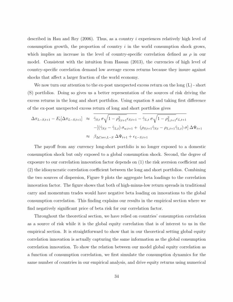
described in Hau and Rey (2006). Thus, as a country i experiences relatively high level of

consumption growth, the proportion of country i in the world consumption shock grows,

which implies an increase in the level of country-specific correlation defined as ρ in our

model. Consistent with the intuition from Hassan (2013), the currencies of high level of

country-specific correlation demand low average excess returns because they insure against

shocks that affect a larger fraction of the world economy.

We now turn our attention to the ex-post unexpected excess return on the long (L) - short

(S) portfolios. Doing so gives us a better representation of the sources of risk driving the

excess returns in the long and short portfolios. Using equation 8 and taking first difference

of the ex-post unexpected excess return of long and short portfolios gives

∆πL−S,t+1 − Et[∆πL−S,t+1] ≈ γS,t σ√

1− ρ2S,t+1εS,t+1 − γL,t σ

√1− ρ2

L,t+1εL,t+1

−[(γS,t − γL,t) σw,t+1 + (ρS,t+1γS,t − ρL,t+1γL,t) σ] ∆Ψt+1

≈ β∆Corr,L−S ∆Ψt+1 + εL−S,t+1

The payoff from any currency long-short portfolio is no longer exposed to a domestic

consumption shock but only exposed to a global consumption shock. Second, the degree of

exposure to our correlation innovation factor depends on (1) the risk aversion coefficient and

(2) the idiosyncratic correlation coefficient between the long and short portfolios. Combining

the two sources of dispersion, Figure 9 plots the aggregate beta loadings to the correlation

innovation factor. The figure shows that both of high-minus-low return spreads in traditional

carry and momentum trades would have negative beta loading on innovations to the global

consumption correlation. This finding explains our results in the empirical section where we

find negatively significant price of beta risk for our correlation factor.

Throughout the theoretical section, we have relied on countries’ consumption correlation

as a source of risk while it is the global equity correlation that is of interest to us in the

empirical section. It is straightforward to show that in our theoretical setting global equity

correlation innovation is actually capturing the same information as the global consumption

correlation innovation. To show the relation between our model global equity correlation as

a function of consumption correlation, we first simulate the consumption dynamics for the

same number of countries in our empirical analysis, and drive equity returns using numerical

34

integration.28 A time-series of the global consumption correlation level is given by the

equation for Ψt+1 and that of the global equity correlation level is estimated by running the

DECO model on the simulated equity return series. Figure 10 plots the time-series of the

global consumption levels and innovations (solid blue line) and the equity correlation levels

and innovations (dotted red lines) in the upper and lower panel, respectively. The figure

shows that they are essentially measuring the same thing, hence using equity correlation in

the empirical setting is motivated by our model.

6 Conclusion

Carry and momentum trades are a widely known strategies in the FX markets. As the

strategies draw more attention from global investors, there have been recent developments to

create benchmark indices and ETFs reflecting this popularity in FX carry and momentum.

These strategies have also received a great deal of attention in the academic literature to

explain their abnormal profitability. Despite this popularity, the risk based explanations in

the literature have not been very successful in simultaneously explaining their returns. In this

paper, we build a factor which governs the evolution of co-movements in the international

equity markets and show that it explains the cross-sectional differences in the excess return of

carry and momentum portfolios. We find that FX portfolios which deliver high average excess

returns are negatively related to innovations in the global equity correlation. The differences

in exposure to our correlation factor can explain the systematic variation in average excess

returns of portfolios sorted on interest rates and past returns simultaneously. Furthermore,

we derive the condition under which investors should demand high compensation for bearing

the global correlation risk. From the decomposition of FX risk premia, we show that the

cross-sectional differences in loading on the correlation factor depend on two conditions, the

risk aversion coefficient and the country-specific correlation. We demonstrate that carry

portfolios are closely related to the former term, whereas momentum portfolios are closely

related to the latter term. Taking both terms together, we show that the payoffs from both

carry and momentum trades positively co-move with our global correlation innovation.

28See, Watcher (2005) for details of the numerical integration methodology.

35

While a large body of the FX literature explores the linkages between economic funda-

mentals and carry and momentum strategies, our global equity correlation factor bridges

both the FX and international equity markets. By showing that a factor constructed from

the international equity market can explain abnormal returns in the FX market, we shed

light on the cross-market integration where premiums in two different markets are driven by

the same aggregate risk. A useful extension of this study would be to investigate the role of

currency risk in equity market contagion. Identifying crisis and non-crisis periods through

our global correlation factor may help to link a contagion indicator in one market to the

other market. We leave this cross-market contagion for future research.

36

A Appendices

A.1 DECO model

The following section illustrates the DECO model. To standardize the individual equity

return series, we assume the return and the conditional variance dynamics of equity index i

at time t are given by

ri,t = µi + εi,t = µi + σi,tzi,t (9)

σ2i,t = ωi + αiε

2i,t−1 + βiσ

2i,t−1 (10)

where µi denotes the unconditional mean, σ2i,t the conditional variance, zi,t a standard normal

random variable, ωi the constant term, αi the sensitivity to the squared innovation, and βi

the sensitivity to the previous conditional variance. Since the covariance is just the product of

correlations and standard deviations, we can write the covariance matrix (Σt) of the returns

at time t as Σt = DtRtDt where Dt has the standard deviations (σi,t) on the diagonal and

zero elsewhere, and Rt is an n×n conditional correlation matrix of standardized returns (zt)

at time t. Depending on the specification of the dynamics of the correlation matrix, DCC

correlation (RDCCt ) and DECO correlation (RDECO

t ) can be separated. Let Qt denotes the

conditional covariance matrix of zt.

Qt = (1− αQ − βQ)Q+ αQQ12t−1zt−1z

′

t−1Q12t−1 + βQQt−1 (11)

RDCCt = Q

− 12

t QtQ− 1

2t (12)

ρt =1

n(n− 1)(ı

′RDCCt ı− n) (13)

RDECOt = (1− ρt)In + ρtJn×n (14)

where αQ is the sensitivity to the covariance innovation of zt, βQ is the sensitivity to the

previous conditional covariance of zt, Qt replaces the off-diagonal elements of Qt with zeros

but retains its main diagonal, Q is the unconditional covariance matrix of zt, ρt is the

equicorrelation, ı is an n × 1 vector of ones, In is the n-dimensional identity matrix, and

Jn×n is an n×n matrix of ones. To estimate our model, we follow the methodology in Engle

and Kelly (2012). We refer the reader to the latter paper for an exhaustive description of

the estimation methodology.

37

A.2 Cross-sectional asset pricing model

Let f be a K-vector of factors, R be a vector of returns on N test assets with mean µR

and covariance matrix VR, and β be the N ×K matrix of multiple regression betas of the

N assets with respect to the K factors. Let Yt = [f′t , R

′t]

′be an N + K vector. Denote the

mean and variance of Yt as

µ = E[Yt] =

µf

µR

V = V ar[Yt] =

Vf VfR

VRf VR

If the K factor asset pricing model holds, the expected returns of the N assets are given by

µR = Xγ, where X = [1N , β] and γ = [γ0, γ′1]

′is a vector consisting of the zero-beta rate and

risk premia on the K factors. In a constant beta case, the two-pass cross-sectional regression

(CSR) method first obtains estimates β by running the following multivariate regression:

Rt = α + βft + εt, t = 1, · · · , T

β = VRf V−1f

γW = argminγ(µR −Xγ)′W (µR −Xγ) = (X

′WX)−1X

′WµR

γ = (X′WX)−1X

′WµR

where W = IN under OLS CSR and W = Σ−1 = (VR − VRfV −1f VfR)−1 under GLS CSR (or

equivalently use W = V −1R ).

A normalized goodness-of-fit measure of the model (cross-sectional R2) can be defined as

ρ2W = 1 − Q

Q0, where Q = e′WWeW , Q0 = e′0We0, eW = [IN − X(X

′WX)−1X

′W ]µR, and

e0 = [IN − 1N(1′NW1N)−11

′NW ]µR.

Shanken (1992) provides asymptotic distribution of γ adjusted for the errors-in-variables

problem accounting for the estimation errors in β. For OLS CSR, and GLS CSR,

√T (γ − γ)

A∼ N(0K+1, (1 + γ′V −1f γ)(X

′X)−1(X

′ΣX)(X

′X)−1 +

0 0′K

0K Vf

38

√T (γ − γ)

A∼ N(0K+1, (1 + γ′V −1f γ)(X

′ΣX)−1 +

0 0′K

0K Vf

Kan, Robotti, and Shanken (2013) further investigate the asymptotic distribution of γ

under potentially misspecified models as well as under the case when the factors and returns

are i.i.d. multivariate elliptically distribution. The distribution is given by

√T (γ − γ)

A∼ N(0K+1, V (γ))

V (γ) =∞∑

j=−∞

E[hth′

t+j]

ht = (γt − γ)− (θt − θ)wt +Hzt

where θt = [γ0t, (γ1t− ft)′]′, θ = [γ0, (γ1− µf )

′]′, ut = e′W (Rt− µR), wt = γ

′1V−1f (ft− µf ),

and zt = [0, ut(ft − µf )′V −1f ]

′. Note that the term ht is now specified with three terms

which are the asymptotic variance of γ when the true β is used, the errors-in-variables (EIV)

adjustment term, and the misspecification adjustment term. Please see Kan, Robotti, and

Shanken (2013) for details of the estimation.

An alternative specification will be in terms of the N × K matrix VRf of covariances

between returns and the factors.

µR = Xγ = Cλ (15)

λ = (C′WC)−1C

′WµR (16)

where C = [1N , VRF ] and λW = [λW,0, λ′W,1]

′.

Although the pricing errors from this alternative CSR are the same as those in the

one using β above (thus the cross-sectional R2 will also be the same), they emphasize the

differences in the economic interpretation of the pricing coefficients. In fact, according to

the paper, what matter is whether the price of covariance risk associated additional factors

is nonzero if we want to answer whether the extra factors improve the cross-sectional R2.

Therefore, we apply both tests based on λ as well as β in the empirical testing. They also

have shown how to use the asymptotic distribution of the sample R2 (ρ) in the second-pass

CSR as the basis for a specification test. Testing ρ also crucially depends on the value of ρ.

39

References

Akram, F., Rime, D., Sarno, L., 2008. Arbitrage in the foreign exchange market: Turning on themicroscope. Journal of International Economics 76, 237–253.

Ang, A., Chen, J., 2002. Asymmetric Correlations of Equity Portfolios. Journal of Financial Eco-nomics 63, 443–494.

Asness, C. S., Moskowitz, T. J., Pedersen, L. H., 2013. Value and Momentum Everywhere. Journalof Finance 68, 929–985.

Bakshi, G., Panayotov, G., 2013. Predictability of Currency Carry Trades and Asset Pricing Im-plications. Journal of Financial Economics 110, 139–163.

Bansal, R., Shaliastovich, I., 2012. A Long-Run Risks Explanation of Predictability Puzzles inBond and Currency Markets. National Bureau of Economic Research Working Paper.

Bekaert, G., Harvey, C. R., 1995. Time-Varying World Market Integration. Journal of Finance 50,403–444.

Bekaert, G., Harvey, C. R., Lundblad, C., Siegel, S., 2007. Global Growth Opportunities andMarket Integration. Journal of Finance 62, 1081–1137.

Brunnermeier, M. K., Nagel, S., Pedersen, L. H., 2008. Carry Trades and Currency Crashes. NBERMacroeconomics Annual 2008 23, 313–347.

Burnside, C., Eichenbaum, M., Kleshchelski, I., Rebelo, S., 2011a. Do Peso Problems Explain theReturns to the Carry Trade? Review of Financial Studies 24(3), 853–891.

Burnside, C., Eichenbaum, M., Rebelo, S., 2011b. Carry Trade and Momentum in Currency Mar-kets. Annual Review of Financial Economics 3, 511–535.

Campbell, J. Y., Cochrane, J. H., 1999. By Force of Habit: A Consumption-Based Explanation ofAggregate Stock Market Behavior. Journal of Political Economy 107, 205–251.

Campbell, J. Y., Giglio, S., Polk, C., Turley, R., 2013. An Intertemporal CAPM with StochasticVolatility. Working Paper .

Christoffersen, P., Du, D., Elkamhi, R., 2015. Rare Disasters and Credit Market Puzzles. WorkingPaper .

Driessen, J., Maenhout, P. J., Vilkov, G., 2009. The Price of Correlation Risk: Evidence fromEquity Options. Journal of Finance 64, 1377–1406.

Engle, R., 2002. Dynamic Conditional Correlation: A Simple Class of Multivariate GARCH Models.Journal of Business and Economic Statistics 20, 339–350.

Engle, R., Kelly, B., 2012. Dynamic Equicorrelation. Journal of Business and Economic Statistics30, 212–228.

40

Evans, M. D., Lyons, R. K., 2002a. Order Flow and Exchange Rate Dynamics. Journal of PoliticalEconomy 110, 170–180.

Evans, M. D., Lyons, R. K., 2002c. Informational Integration and FX Trading. Journal of Interna-tional Money and Finance 21, 807–831.

Farhi, E., Fraiberger, S. P., Gabaix, X., Ranciere, R., Verdelhan, A., 2009. Crash Risk in CurrencyMarkets. National Bureau of Economic Research Working Paper.

Hansen, L. P., 1982. Large Sample Properties of Generalized Method of Moments Estimators.Econometrica 50, 1029–1054.

Hansen, L. P., Hodrick, R. J., 1980. Forward Exchange Rates as Optimal Predictors of Future SpotRates: An Econometric Analysis. Journal of Political Economy 88, 829–853.

Harvey, C. R., Siddique, A., 2000. Conditional Skewness in Asset Pricing Tests. Journal of Finance55, 1263–1296.

Hassan, T. A., 2013. Country Size, Currency Unions, and International Asset Returns. Journal ofFinance 68, 2269–2308.

Hau, H., Rey, H., 2006. Exchange Rates, Equity Prices, and Capital Flows. Review of FinancialStudies 19, 273–317.

Herskovic, B., Kelly, B. T., Lustig, H. N., Nieuwerburgh, S. V., 2014. The Common Factor inIdiosyncratic Volatility: Quantitative Asset Pricing Implications. Journal of Financial Economicsforthcoming.

Hong, Y., Tu, J., Zhou, G., 2007. Asymmetries in Stock Returns: Statistical Tests and EconomicEvaluation. Review of Financial Studies 20, 1547–1581.

Jurek, J. W., 2014. Crash Neutral Currency Carry Trades. JFE forthcoming .

Kan, R., Robotti, C., Shanken, J. A., 2013. Pricing Model Performance and the Two-Pass Cross-Sectional Regression Methodology. Journal of Finance 68, 2617–2649.

Kan, R., Zhang, C., 1999. Two-Pass Tests of Asset Pricing Models with Useless Factors. Journalof Finance 54, 203–235.

Lettau, M., Maggiori, M., Weber, M., 2014. Condisional risk premia in currency markets and otherasset classes. Journal of Financial Economics 114, 197–225.

Lustig, H., Roussanov, N., Verdelhan, A., 2011. Common Risk Factors in Currency Markets. Reviewof Financial Studies 24, 3731–3777.

Lustig, H., Roussanov, N., Verdelhan, A., 2014. Countercyclical Currency Risk Premia. Journal ofFinancial Economics 111, 527–553.

41

Lustig, H., Verdelhan, A., 2007. The Cross-Section of Foreign Currency Risk Premia and Consump-tion Growth Risk. American Economic Review 97, 89–117.

Mancini, L., Ranaldo, A., Wrampelmeyer, J., 2013. Liquidity in the Foreign Exchange Market:Measurement, Commonality, and Risk Premiums. Journal of Finance 68, 1805–1841.

Menkhoff, L., Sarno, L., Schmeling, M., Schrimpf, A., 2012a. Carry Trades and Global ForeignExchange Volatility. Journal of Finance 67, 681–718.

Menkhoff, L., Sarno, L., Schmeling, M., Schrimpf, A., 2012b. Currency Momentum Strategy. Jour-nal of Financial Economics 106, 660–684.

Menzly, L., Santos, T., Veronesi, P., 2004. Understanding Predictability. Journal of Political Econ-omy 112, 1–47.

Merton, R. C., 1973. An Intertemporal Capital Asset Pricing Model. Econometrica 41, 867–887.

Moskowitz, T. J., Ooi, Y. H., Pedersen, L. H., 2012. Time Series Momentum. Journal of FinancialEconomics 104, 228–250.

Newey, W. K., West, K. D., 1987. A Simple, Positive Semi-Definite Heteroskedasticity and Auto-correlation Consistent Covariance Matrix. Econometrica 55, 703–708.

Okunev, J., White, D., 2003. Do Momentum-Based Strategies Still Work in Foreign CurrencyMarkets? Journal of Financial and Quantitative Analysis 38, 425–447.

Pastor, L., Stambaugh, R. F., 2003. Liquidity Risk and Expected Stock Returns. Journal of PoliticalEconomy 111, 642–685.

Patton, A. J., Timmermann, A., 2010. Monotonicity in Asset Returns: New Tests with Applicationsto the Term Structure, the CAPM and Portfolio Sorts. Journal of Financial Economics 98, 605–625.

Pollet, J. M., Wilson, M., 2010. Average Correlation and Stock Market Returns. Journal of FinancialEconomics 96, 364–380.

Roll, R., 1977. A critique of the asset pricing theory’s tests Part I: On past and potential testabilityof the theory. Journal of Financial Economics 4, 129–176.

Shanken, J., 1992. On the Estimation of Beta Pricing Models. Review of Financial Studies 5, 1–55.

Verdelhan, A., 2010. A Habit-Based Explanation of the Exchange Rate Risk Premium. Journal ofFinance 65, 123–146.

Watcher, J. A., 2005. Solving models with external habit. Finance Research Letters 2, 210–226.

42

19

78

19

82

19

86

19

90

19

94

19

98

20

02

20

06

20

10

20

14

0

0.2

0.4

0.6

0.81

Co

rre

lati

on

Le

ve

ls

DE

CO

IS

DE

CO

OO

S (

OO

S)

Intr

a−

mo

nth

(IM

)

19

78

19

82

19

86

19

90

19

94

19

98

20

02

20

06

20

10

20

14

−0

.50

0.5

Co

rre

lati

on

In

no

va

tio

ns

Fig

ure

1:C

orr

ela

tion

Innovati

on

Fact

ors

Th

eu

pp

erp

anel

ofth

efi

gure

show

sa

tim

e-se

ries

plo

tof

the

glo

bal

equ

ity

corr

elati

on

leve

ls.

Th

eso

lid

bla

ckli

ne,

DE

CO

IS,

ism

easu

red

by

DE

CO

mod

el(E

ngl

ean

dK

elly

,20

12)

wh

ere

para

met

ers

are

esti

mate

don

the

enti

rem

onth

lyre

turn

seri

esof

inte

rnati

on

al

ind

ices

.T

he

soli

dgr

ayli

ne,

DE

CO

OO

S(o

ut-

of-s

amp

le),

ism

easu

red

by

the

sam

em

od

elw

her

ep

ara

met

ers

are

esti

mate

don

the

data

avail

ab

leon

ly

atth

ep

oint

inti

me

and

up

dat

edw

ith

exp

an

din

gw

ind

owas

we

coll

ect

more

data

.T

he

dott

edre

dlin

e,co

rrel

ati

on

leve

lis

mea

sure

dby

com

pu

tin

gb

ilat

eral

intr

a-m

onth

(IM

)co

rrel

ati

on

sat

each

month

’sen

du

sin

gd

ail

yre

turn

seri

es.

Th

en,

we

take

an

aver

age

of

all

the

bil

ater

alco

rrel

atio

ns

toar

rive

agl

obal

corr

elati

on

leve

lof

ap

art

icu

lar

month

.T

he

low

erp

an

elsh

ows

ati

me-

seri

esp

lot

of

the

glo

bal

equ

ity

corr

elat

ion

inn

ovat

ion

s.T

he

corr

elat

ion

inn

ovati

on

sare

mea

sure

dby

takin

gfi

rst

diff

eren

ceof

each

of

the

corr

elati

on

leve

ls.

The

sam

ple

cove

rsth

ep

erio

dM

arch

1976

toD

ecem

ber

2014.

43

Portfolios

1 2 3 4 5−0.04

−0.03

−0.02

−0.01

0

0.01

0.02

0.03

0.04D. Momentum 5: Beta Loadings

1 2 3 4 5−0.04

−0.03

−0.02

−0.01

0

0.01

0.02

0.03

0.04C. Carry 5: Beta Loadings

Beta

Loadin

gs

1 2 3 4 5−2

0

2

4

6

8B. Momentum 5: Average Excess Return

1 2 3 4 5−2

0

2

4

6

8A. Carry 5: Average Excess Return

Avera

ge E

xcess R

etu

rn

Figure 2: Average Excess Returns and Beta LoadingsThis figure plots the average excess returns of carry and momentum portfolios in Panel A andB, and each portfolio’s beta loading with respect to our global equity correlation innovationfactor in Panel C and D. The aggregate correlation levels are measured by out-of-sampleDECO model (OOS ) as described in Section 4.1. The sample covers the period May 1976to December 2014.

44

Pre

dic

ted m

ean e

xcess r

etu

rns

Realized mean excess returns (in % per annum)

−2 0 2 4 6 8−2

−1

0

1

2

3

4

5

6

7

8A. DOL + DECO OOS (R

2 = 0.89)

Carry

MoM

−2 0 2 4 6 8−3

−2

−1

0

1

2

3

4

5

6

7

8B. DOL + Intra−month (R

2 = 0.82)

Carry

MoM

Figure 3: Pricing Error Plot: Correlation Innovation Factors on FX 10This figure presents the pricing errors of the asset pricing models with our global equitycorrelation as a risk factor. The global equity correlation levels are measured by DECO model(OOS) for Panel A and by averaging intra-month bilateral correlations (IM) for Panel B.The realized actual excess returns are on the horizontal axis and the model predicted averageexcess returns are on the vertical axis. The test assets are FX 10 portfolios: the set of carryportfolios (5) and momentum portfolios (5). The estimation results are based on OLS CSRtest while imposing the same price of risk for the test assets within each plot. The samplecovers the period March 1976 to December 2014.

45

19

78

19

82

19

86

19

90

19

94

19

98

20

02

20

06

20

10

20

14

−0

.20

0.2

0.4

0.6

0.81

1.2

A.

Co

rre

lati

on

Le

ve

ls

Intr

a−

mo

nth

(IM

)

Intr

a−

mo

nth

(IM

GD

P)

Intr

a−

mo

nth

(IM

MK

T)

19

78

19

82

19

86

19

90

19

94

19

98

20

02

20

06

20

10

20

14

−0

.8

−0

.6

−0

.4

−0

.20

0.2

0.4

0.6

B.

Co

rre

lati

on

In

no

va

tio

ns

Fig

ure

4:D

iffere

nt

Weig

hti

ngs

for

the

Glo

bal

Corr

ela

tion

Innovati

on

Fact

or

Th

eu

pp

erp

anel

ofth

efi

gure

show

sa

tim

e-se

ries

plo

tof

the

glo

bal

equ

ity

corr

elati

on

leve

ls.

Inea

chm

onth

end

,co

rrel

ati

on

leve

lsare

mea

sure

dby

com

pu

tin

gb

ilat

eral

intr

a-m

onth

corr

elati

on

sat

each

month

end

usi

ng

dail

yre

turn

seri

esof

inte

rnat

ion

al

MS

CI

equ

ity

ind

ices

.

Th

eso

lid

bla

ckli

ne,IM

,th

eag

greg

ate

corr

elati

on

leve

lis

esti

mate

dby

com

pu

tin

geq

uall

y-w

eighte

dav

erage

over

all

bil

ate

ral

corr

elati

on

s

atth

een

dof

each

mon

th.

Th

egr

ay(d

otte

dre

d)

lin

e,IM

GDP

(IM

MK

T),

corr

elati

on

leve

lsare

esti

mate

dby

com

pu

tin

gG

DP

-wei

ghte

d

(Mar

ket-

cap

ital

izat

ion

-wei

ghte

d)

aver

age

over

all

bil

ate

ral

corr

elati

on

s.T

he

low

erp

an

elsh

ows

ati

me-

seri

esp

lot

of

the

glo

bal

equ

ity

corr

elat

ion

inn

ovat

ion

s.T

he

corr

elat

ion

inn

ovati

on

sare

mea

sure

dby

takin

gfi

rst

diff

eren

ceof

each

of

the

corr

elati

on

leve

ls.

The

sam

ple

cove

rsth

ep

erio

dM

arch

1976

toD

ecem

ber

2014.

46

Pre

dic

ted

me

an

exce

ss r

etu

rns

Realized mean excess returns (in % per annum)

−2 0 2 4 6 8

−2

0

2

4

6

8A. Equity Corr Innovation (R

2 = 0.89)

Carry

Momentum

−2 0 2 4 6 8

−2

0

2

4

6

8B. FX Vol Innovation (R

2 = 0.68)

Carry

Momentum

−2 0 2 4 6 8

−2

0

2

4

6

8C. FX Corr Innovation (R

2 = 0.5)

Carry

Momentum

−2 0 2 4 6 8

−2

0

2

4

6

8D. HML Carry (R

2 = 0.72)

Carry

Momentum

−2 0 2 4 6 8

−2

0

2

4

6

8E. HML Momentum (R

2 = 0.55)

Carry

Momentum

−2 0 2 4 6 8

−2

0

2

4

6

8F. Global CAPM (R

2 = 0.43)

Carry

Momentum

Figure 5: Pricing Error Plot: Other FactorsThe figure presents the pricing errors of the asset pricing models with the selected risk factorsfrom the list described in Section 4.4. The realized actual excess returns are on the horizontalaxis and the model predicted average excess returns are on the vertical axis. The test assetsare FX 10 portfolios: the set of carry portfolios (5) and momentum portfolios (5). We use ourglobal equity correlation innovation factor (OOS) in Panel A, the FX volatility innovationfactor in Panel B, the FX correlation innovation factor in Panel C, the high-minus-low carryfactor in Panel D, the high-minus-low momentum factor in Panel E, and the global equitymarket factor in Panel F. The estimation results are based on OLS CSR test. The samplecovers the period March 1976 to December 2014.

47

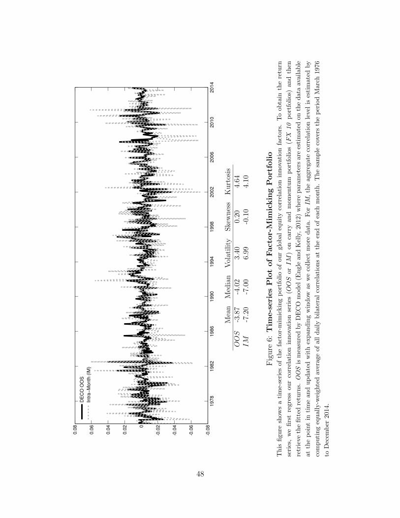
19

78

19

82

19

86

19

90

19

94

19

98

20

02

20

06

20

10

20

14

−0

.08

−0

.06

−0

.04

−0

.020

0.0

2

0.0

4

0.0

6

0.0

8

DE

CO

OO

S

Intr

a−

Mo

nth

(IM

)

Mea

nM

edia

nV

olat

ilit

ySke

wnes

sK

urt

osis

OOS

-3.8

7-4

.02

3.40

0.20

4.64

IM

-7.2

0-7

.00

6.99

-0.1

04.

10

Fig

ure

6:T

ime-s

eri

es

Plo

tof

Fact

or-

Mim

ickin

gP

ort

foli

oT

his

figu

resh

ows

ati

me-

seri

esof

the

fact

or-

mim

ickin

gp

ort

foli

oof

ou

rglo

bal

equ

ity

corr

elati

on

inn

ovati

on

fact

ors

.T

oob

tain

the

retu

rn

seri

es,

we

firs

tre

gres

sou

rco

rrel

atio

nin

nov

ati

on

seri

es(OOS

orIM

)on

carr

yand

mom

entu

mp

ort

foli

os

(FX

10

port

foli

os)

an

dth

en

retr

ieve

the

fitt

edre

turn

s.O

OS

ism

easu

red

by

DE

CO

mod

el(E

ngle

an

dK

elly

,2012)

wh

ere

para

met

ers

are

esti

mate

don

the

data

avail

ab

le

atth

ep

oint

inti

me

and

up

dat

edw

ith

exp

an

din

gw

ind

owas

we

coll

ect

more

data

.F

or

IM,

the

aggre

gate

corr

elati

on

level

ises

tim

ate

dby

com

pu

tin

geq

ual

ly-w

eigh

ted

aver

age

ofal

ld

ail

yb

ilate

ral

corr

elati

on

sat

the

end

of

each

month

.T

he

sam

ple

cove

rsth

ep

erio

dM

arc

h1976

toD

ecem

ber

2014

.

48

Pre

dic

ted

me

an

exce

ss r

etu

rns

Realized mean excess returns (in % per annum)

−2 0 2 4 6 8−2

0

2

4

6

8A. Carry

−2 0 2 4 6 8−2

0

2

4

6

8B. Momentum

−2 0 2 4 6 8−2

0

2

4

6

8C. Value (REER)

−2 0 2 4 6 8−2

0

2

4

6

8D. Long rate (10Y)

−2 0 2 4 6 8−2

0

2

4

6

8E. Momentum (6M)

−2 0 2 4 6 8−2

0

2

4

6

8

F. Value ( ∆ REER)

Figure 7: Pricing Error Plot: Factor-Mimicking PortfolioThe figure shows the pricing errors of the asset pricing models with a factor-mimickingportfolio of our correlation innovation (OOS ) as a risk factor. The realized actual excessreturns are on the horizontal axis and the model predicted average excess returns are on thevertical axis. The test assets are five portfolios sorted on A. Carry: short-term (1M) interestrate differentials, B. Momentum: past three-months excess returns, C. Value (REER): thelevel of real effective exchange rates, D. Long rate: long-term (10Y) interest rate differentials,E. Momentum (6M): past 6-month excess returns, and F. Value (∆REER): past 60-monthchanges of real effective exchange rates. The estimation results are based on OLS CSR test.The sample covers the period March 1976 to December 2014.

49

0 20 40 60 80 100 120 140 160 180 2001

1.5

2

2.5

3

3.5

4

4.5

5

γ

A. Carry Portfolio γ

Low Interest

High Interest

0 20 40 60 80 100 120 140 160 180 2001

1.5

2

2.5

3

3.5

4

4.5

5

γ

B. Momentum Portfolio γ

Low Momentum

High Momentum

0 20 40 60 80 100 120 140 160 180 200−4

−3

−2

−1

0

1

2

3

4

ργ

C. Carry Portfolio ργ

Low Interest

High Interest

0 20 40 60 80 100 120 140 160 180 200−4

−3

−2

−1

0

1

2

3

4

ργ

D. Momentum Portfolio ργ

Low Momentum

High Momentum

Figure 8: Simulated Parameters for Carry and Momentum PortfoliosThis figure shows the simulated parameters for carry and momentum portfolios. Panel A andC (B and D) show the average values of the parameters for carry (momentum) portfolios.We show a time-series plot of γ in the upper panels (Panel A and B), and a time-series plotof ργ in the lower panels (Panel C and D) respectively. In each panel, the solid blue line isa time-series plot of the parameter values for a low interest (momentum) portfolio, and thedotted black line is for a high interest (momentum) portfolio.

50

0 20 40 60 80 100 120 140 160 180 200−14

−12

−10

−8

−6

−4

−2

0

A. HML Carry Trades

0 20 40 60 80 100 120 140 160 180 200−20

−18

−16

−14

−12

−10

−8

−6

−4

−2

0

B. HML Momentum Trades

Figure 9: Beta Loadings to the Correlation Innovation FactorThe figure on the left shows a time-series of beta loadings to the correlation innovationfactor of HML carry trades: long high interest rate currencies and short low interest ratecurrencies, using simulated rates and returns. The figure on the right shows those of HMLmomentum trades: long high excess return currencies and short excess return currenciesover the last three month, using simulated returns. In other words, the solid blue lineplots β∆Corr,L−S of the equation below for the long-short carry trades (Panel A) and for thelong-short momentum trades (Panel B).

∆πL−S,t+1 − Et[∆πL−S,t+1] ≈ γS,t σ√

1− ρ2S,t+1εS,t+1 − γL,t σ

√1− ρ2

L,t+1εL,t+1

−[(γS,t − γL,t) σw,t+1 + (ρS,t+1γS,t − ρL,t+1γL,t) σ] ∆Ψt+1

≈ β∆Corr,L−S ∆Ψt+1 + εL−S,t+1

51

0 20 40 60 80 100 120 140 160 180 2000.35

0.4

0.45

0.5

0.55

0.6

0.65

0.7

Correlation Level

Consumption Correlation

Equity Correlation

0 20 40 60 80 100 120 140 160 180 200−0.1

−0.05

0

0.05

0.1

0.15

Correlation Innovation

Consumption Corr Innvation

Equity Corr Innvation

Figure 10: Simulated Consumption and Equity Correlation InnovationThis figure compares consumption correlations and equity correlations where both seriesare simulated from our model. The upper panel of the figure shows a time-series plotof the common consumption correlation levels (solid blue line) and the equity correlationlevels estimated by running DECO model on the simulated equity returns (dotted red line).The lower panel shows a time-series plot of the correlation innovations. The correlationinnovations are measured by taking first difference of each of the correlation levels. Thecorrelations between two series are 0.76 and 0.80 for the level and the innovation respectively.

52

Table 1: Moments of Carry and Momentum Portfolios

The table reports statatistics for the annualized excess currency returns of currency portfolios sorted asfollows. A. Carry portfolios are sorted on last month’s forward discounts with one-month maturity, B.Momentum portfolios on their excess return over the last 3 month. All portfolios are rebalanced at the endof each month and the excess returns are adjusted for transaction costs (bid-ask spread). The portfolio 1contains the 20% of currencies with the lowest the lowest interest differentials (or past returns), while portfolio5 contains currencies with the highest interest differentials (or past returns). HML denotes differences inreturns between portfolio 5 and 1. The excess returns cover the period March 1976 to December 2014.

All Countries (44) Developed Countries (17)

Panel A. Carry: Portfolios Sorted on Forward Discounts

Low 2 3 4 High HML Low 2 3 4 High HML

Mean -1.67 0.10 1.91 3.39 5.10 6.77 -0.88 -0.77 1.25 2.58 4.48 5.37Median -1.49 1.40 2.35 4.75 9.21 9.90 -0.52 1.54 2.41 3.92 5.24 9.39Std. Dev 9.14 9.13 8.45 8.92 10.07 7.95 10.02 9.79 9.08 9.56 10.73 9.33Skewness -0.10 -0.43 0.00 -0.44 -1.05 -1.84 0.05 -0.16 -0.16 -0.42 -0.40 -0.58Kurtosis 4.41 4.66 4.12 4.65 6.99 6.25 3.77 3.90 4.08 5.05 5.00 4.91Sharpe Ratio -0.18 0.01 0.23 0.38 0.51 0.85 -0.09 -0.08 0.14 0.27 0.42 0.58AR(1) 0.03 0.01 0.04 0.07 0.13 0.14 0.00 0.06 0.05 0.03 0.08 0.03

Panel B. Momentum: Portfolios Sorted on Past Excess Returns

Low 2 3 4 High HML Low 2 3 4 High HML

Mean -1.29 -0.18 1.50 2.79 6.29 7.58 -1.32 1.58 1.24 1.84 3.69 5.01Median -0.27 1.27 2.21 3.19 6.46 7.34 -0.49 2.45 2.55 3.21 4.96 6.38Std. Dev 9.63 9.29 9.21 9.00 9.01 8.23 9.90 10.04 10.32 9.85 9.47 9.37Skewness -0.20 -0.40 -0.20 -0.27 -0.26 -0.14 -0.12 -0.18 -0.34 -0.13 -0.14 -0.03Kurtosis 4.67 4.63 4.50 4.16 4.55 3.84 5.18 4.27 4.02 3.90 4.11 4.03Sharpe Ratio -0.13 -0.02 0.16 0.31 0.70 0.92 -0.13 0.16 0.12 0.19 0.39 0.53AR(1) 0.04 0.06 0.01 0.05 0.06 -0.08 0.04 0.04 0.06 0.00 0.02 -0.06

53

Table 2: Cross-Sectional Regression (CSR) TestsThe table reports cross-sectional pricing results for the factor model based on the dollar risk factor (DOL) and

Global Equity Correlation Innovation (∆Corr) where the correlation levels are measured by DECO (OOS)

model for Panel A and by averaging intra-month bilateral correlations (IM) for Panel B, respectively. The

test assets are the set of carry portfolios (1-5), and the set of momentum portfolios (1-5). Table on the left

(right) reports the estimation results for the test assets using currencies from all 44 countries (17 developed

market countries only). The market price of covariance risk λ, the market price of beta risk γ (multiplied

by 100), and the price of covariance (beta) risk normalized by standard deviation of the cross-sectional

covariances (betas): λnorm (γnorm) are reported. Shanken (1992)’s t-ratios under correctly specified models

accounting for the EIV problem: (t-ratios) and the Kan, Robotti, and Shanken (2012) misspecification-robust

t-ratios: (t-ratiokrs) are reported in the parentheses. pval1 is the p-value for the test of H0: R2 = 1. pval2is the p-value for the test of H0: R2 = 0. pval3 is the p-value for Wald test of H0: γ = 0K without imposing

price of beta is zero under the null. pval4 is the p-value for approximate finite sample p-value of Shanken’s

CSRT statistic (a generalized χ2-test). Data are monthly and the sample covers the period May 1976 to

December 2014.

All Countries (44) Developed Countries (17)

Panel A. DECO (OOS)

Factor: DOL ∆CorrOOS Factor: DOL ∆CorrOOS

λ 2.28 -35.85 R2 0.89 λ 1.52 -19.00 R2 0.77λnorm 0.07 -2.56 pval1 [0.55] λnorm 0.08 -1.65 pval1 [0.36]

t-ratiofm (1.16) (-7.94) pval2 [0.00] t-ratiofm (0.76) (-4.57) pval2 [0.02]t-ratios (0.56) (-3.74) pval3 [0.00] t-ratios (0.55) (-3.24) pval3 [0.02]t-ratiokrs (0.46) (-2.95) pval4 [0.71] t-ratiokrs (0.49) (-2.53) pval4 [0.28]

γ 0.22 -9.37 γ 0.13 -4.97γnorm 0.12 -2.59 γnorm 0.12 -1.66

t-ratiokrs (1.81) (-3.39) t-ratiokrs (1.15) (-2.99)

Panel B. Intra-month (IM)

Factor: DOL ∆CorrIM Factor: DOL ∆CorrIM

λ -1.50 -18.70 R2 0.82 λ -0.29 -8.83 R2 0.67λnorm -0.05 -2.39 pval1 [0.55] λnorm -0.01 -1.40 pval1 [0.34]

t-ratiofm (-0.74) (-7.89) pval2 [0.00] t-ratiofm (-0.14) (-4.15) pval2 [0.02]t-ratios (-0.30) (-3.20) pval3 [0.01] t-ratios (-0.10) (-2.84) pval3 [0.05]t-ratiokrs (-0.27) (-3.48) pval4 [0.72] t-ratiokrs (-0.09) (-2.74) pval4 [0.18]

γ 0.21 -26.38 γ 0.12 -12.47γnorm 0.12 -2.49 γnorm 0.11 -1.45

t-ratiokrs (1.77) (-3.54) t-ratiokrs (1.07) (-2.78)

Description

λ : The price of covariance risk R2 : Sample CSR R-squaredγ : The price of beta risk pval1 : p-value of testing R2 = 1t-ratiofm : Fama-MacBeth t-ratio pval2 : p-value of testing R2 = 0t-ratios : Shanken error-in-variables adjusted t-ratio pval3 : p-value of Wald test γ = 0Kt-ratiokrs : Misspecification robust t-ratio pval4 : p-value of Shanken’s CSRT statistic

54

Table 3: Moments of Correlation Innovation Factors

This table reports statistics for the global equity correlation innovation factors. OOS is measured by DECO

model (Engle and Kelly, 2012) where parameters are estimated on the data available at the point in time and

updated with expanding window as we collect more data. From the second to the third column, the correla-

tion level is measured by computing bilateral intra-month correlations at each month end using daily return

series of international MSCI equity indices in U.S. dollars. For IM , the aggregate correlation level is esti-

mated by computing equally-weighted average of all daily bilateral correlations at the end of each month. For

IMGDP (IMMKT ), the correlation level is estimated by computing GDP-weighted (Market-capitalization-

weighted) average over all bilateral correlations. For IMLOC , daily return series of international MSCI

equity indices in local currency units are used to compute bilateral intra-month correlations, and we take

equally-weighted averages for the aggregation at each month end. The correlation innovations are measured

by taking first difference of each of the correlation levels. The sample covers the period March 1976 to

December 2014.

A. Correlation Level

OOS IM IMGDP IMMKT IMLOC

Mean 0.39 0.39 0.27 0.27 0.33Volatility 0.17 0.19 0.17 0.17 0.21Correlation

IM 0.94IMGDP 0.79 0.84IMMKT 0.75 0.79 0.97IMLOC 0.83 0.81 0.71 0.67

B. Correlation Innovation

OOS IM IMGDP IMMKT IMLOC

Mean 0.00 0.00 0.00 0.00 0.00Volatility 0.05 0.12 0.16 0.17 0.13Correlation

IM 0.77IMGDP 0.50 0.61IMMKT 0.45 0.55 0.96IMLOC 0.51 0.63 0.48 0.45

55

Table 4: Alternative Cross-Sectional Asset Pricing Tests

This table reports the price of beta risk (γ) for the global equity correlation innovation factors from the

various forms of asset pricing models. The test assets are FX 10 portfolios: the set of carry and momentum

portfolios. CSR-OLS (CSR-GLS ) is the two-pass cross-sectional OLS (GLS ) regression. In the first pass,

we run time-series regressions to estimate each asset’s beta to the risk factors. In the second pass, we

run cross-sectional regression where all assets’ average returns are regressed against the estimated betas to

determine the risk premium of each factor. For Fama-MacBeth Constant, the first pass regression is the same

as CSR-OLS. However, in the second pass, we run cross-sectional regressions at each time period. The risk

premium of each factor is determined to be the average price of risk across time. For Fama-MacBeth Rolling

60M, the second pass regression is the same as Fama-MacBeth Constant. However, in the first pass, we run

time-series regressions with rolling 60 months window to estimate each asset’s time-varying beta to the risk

factors. For GMM, we measure the price of risk by specifying the pricing kernel to be linear function of the

risk factors (see, Section 4.3). The misspecification robust t-ratios from Kan, Robotti, and Shanken (2013,

JF) are reported in the parentheses for CSR-OLS and CSR-GLS. The heteroskedasticity and autocorrelation

adjusted t-ratio with automatic lag selection from Newey-West (1994, RES) are reported in the parentheses

for Fama-MacBeth and GMM. The description of the factors is the same as Table 3. The sample covers the

period March 1976 to December 2014.

1. OOS 2. IM 3. GDP 4. MKT 5. LOC

DOL OOS DOL IM DOL IMGDP DOL IMMKT DOL IMLOC

A. CSR - OLS

γ 0.22 -9.37 0.21 -26.38 0.19 -63.03 0.17 -60.49 0.19 -19.92γnorm 0.12 -2.59 0.12 -2.49 0.10 -2.47 0.09 -2.39 0.10 -1.89t-ratiokrs (1.81) (-3.39) (1.77) (-3.54) (1.53) (-1.95) (1.39) (-2.01) (1.66) (-2.93)

B. CSR - GLS

γ 0.20 -8.22 0.19 -20.68 0.17 -42.66 0.15 -43.51 0.16 -12.83γnorm 0.11 -2.27 0.10 -1.96 0.09 -1.67 0.08 -1.72 0.09 -1.22t-ratiokrs (1.72) (-3.08) (1.62) (-2.92) (1.45) (-1.85) (1.34) (-1.79) (1.44) (-2.20)

C. Fama-MacBeth Constant

γ 0.22 -9.37 0.21 -26.38 0.19 -63.03 0.17 -60.49 0.19 -19.92γnorm 0.12 -2.59 0.12 -2.49 0.10 -2.47 0.09 -2.39 0.10 -1.89t-rationw (1.87) (-7.71) (1.80) (-7.80) (1.64) (-7.84) (1.45) (-7.67) (1.68) (-6.03)

D. Fama-MacBeth Rolling 60M

γ 0.17 -3.64 0.17 -7.51 0.19 -5.19 0.19 -6.57 0.21 -8.63γnorm 0.21 -1.61 0.21 -1.45 0.20 -0.61 0.21 -0.71 0.24 -1.45t-rationw (1.27) (-3.68) (1.23) (-3.42) (1.38) (-1.46) (1.39) (-1.64) (1.56) (-2.71)

E. GMM

γ 0.22 -9.26 0.21 -26.11 0.19 -62.66 0.17 -60.18 0.19 -19.77γnorm 0.07 -2.53 -0.04 -2.36 0.06 -2.45 -0.06 -2.26 0.09 -1.84t-rationw (0.48) (-3.27) (-0.31) (-3.84) (0.24) (-2.10) (-0.28) (-2.14) (0.77) (-3.64)

56

Table 5: CSR Tests: Other Factors

This table reports the price of covariance risk (λ) from CSR-OLS from factor models based on the dollar riskfactor (DOL), a control factor, and our global equity correlation innovation factors (OOS). The test assetsare FX 10 portfolios: the set of carry and momentum portfolios. The price of covariance risks normalizedby standard deviation of the cross-sectional covariances (λnorm) are reported. The misspecification-robustt-ratio (t − ratiokrs) from Kan, Robotti, and Shanken (2013, JF) and the p-values for the test of H0 :R2 = 0 are reported in parentheses and in square bracket, respectively. The control factors are described asfollows. ∆FXV OL: the aggregate FX volatility innovationas (Menkhoff, Sarno, Schmeling and Schrimpf, 2012JF), ∆FXCORR: the aggregate FX correlation innovationas, ∆TED: TED spread innovation, ∆FXBAS :innovations to the aggregate FX bid-ask spreads (Mancini, Renaldo and Wrampelmeyer, 2013 JF), ∆LIQPS :Pastor-Stambaugh liquidity innovation, EQMRP : the market risk premium, EQSMB : U.S. equity size factor,EQHML: U.S. equity value factor, EQMOM : U.S. equity momentum factor, CarryHML: the high-minus-low FX carry factor (Lustig, Roussanov, and Verdelhan, 2011 RFS ), MOMHML: the high-minus-low FXmomentum factor.

Factors

ControlStatistics DOL

ControlOOS R2

Factor Factor

A. FX volatility & correlation factors

∆FXV OL λnorm 0.09 0.45 -2.90 0.94t-ratiokrs (0.59) (0.49) (-2.74) [0.00]

∆FXCORR λnorm 0.04 -0.53 -2.30 0.92t-ratiokrs (0.27) (-0.78) (-2.54) [0.00]

B. Liquidity factors

∆TED λnorm 0.12 0.55 -2.83 0.93t-ratiokrs (0.78) (0.86) (-2.91) [0.00]

∆FXBAS λnorm 0.07 0.31 -2.65 0.94t-ratiokrs (0.47) (0.48) (-3.09) [0.00]

∆LIQPS λnorm 0.07 -0.59 -3.03 0.92t-ratiokrs (0.46) (-0.67) (-2.72) [0.00]

C. Equity factors

EQMRP λnorm 0.12 -0.48 -2.78 0.93t-ratiokrs (0.76) (-0.67) (-3.00) [0.00]

EQSMB λnorm 0.06 -0.49 -2.88 0.91t-ratiokrs (0.37) (-0.69) (-2.73) [0.00]

EQHML λnorm 0.10 0.68 -2.33 0.95t-ratiokrs (0.66) (1.27) (-2.64) [0.00]

EQMOM λnorm 0.11 0.63 -2.82 0.94t-ratiokrs (0.72) (0.83) (-2.82) [0.00]

D. FX carry & momentum factors

CarryHML λnorm 0.07 -0.34 -2.81 0.92t-ratiokrs (0.41) (-0.36) (-2.69) [0.00]

MOMHML λnorm 0.08 0.73 -2.13 0.95t-ratiokrs (0.61) (1.04) (-2.39) [0.00]

57

Table 6: CSR Tests: Factor-mimicking Portfolios

The table reports the cross-sectional pricing results for the factor model based on the dollar risk factor(DOL) and our global equity correlation innovation factors: DECO OOS (∆CorrOOS) and intra-monthinnovation (∆CorrIM ) respectively. The factor mimicking portfolios are obtained by projecting the factorsinto FX 10 portfolio space. For Panel A, the test assets are the set of portfolios sorted on last month’sforward discounts (Carry 5 ), their excess returns over the last 3 months (Momentum 5 ), and real effectiveexchange rates (Value 5 ). For Panel B, the test assets are similarly defined as Panel A, but we use 10-yearinterest rate differentials for Carry 5, 6-month excess returns for Momentum 5, and 60-month changes inreal effective exchange rates for Value 5. We report the average annualized returns for HML portfolios (HMLSpread), p-values for the test of H0: HML Spread = 0 (HML Spread p-val), and p-values for the monotonicrelationship test from Patton and Timmermann, 2010 (Monotonicity p-val). We present the price of beta risksnormalized by standard deviation of the cross-sectional betas (γnorm). The misspecification-robust t-ratiosare reported in parentheses (Kan, Robotti, and Shanken, 2012). The p-values for the test of H0 : R2 = 0and H0 : |β5 − β1| = 0 (Patton and Timmermann, 2010) are reported in square bracket.

Panel A Carry 5 Momentum 5 Value 5 (REER)

HML Spread 6.87 7.58 6.34HML Spread p-val [0.00] [0.00] [0.00]

Monotonicity p-val [0.00] [0.00] [0.00]

γnorm R2 Betaγnorm R2 Beta

γnorm R2 Beta

Spread Spread Spread

∆CorrOOS -2.58 0.91 0.06 -2.94 0.91 0.05 -2.00 0.81 0.02(-2.57) [0.00] [0.01] (-3.00) [0.00] [0.01] (-2.37) [0.03] [0.15]

∆CorrIM -2.61 0.93 0.02 -2.83 0.86 0.02 -1.78 0.81 0.01(-1.64) [0.00] [0.04] (-3.36) [0.00] [0.02] (-1.37) [0.04] [0.23]

∆CorrOOS -2.52 0.88 1.54 -2.82 0.87 1.24 -1.16 0.86 0.25(mimicking) (-4.53) [0.00] [0.00] (-5.92) [0.01] [0.00] (-1.60) [0.00] [0.04]

∆CorrIM -2.61 0.90 0.50 -2.83 0.83 0.66 -2.00 0.81 0.19(mimicking) (-3.44) [0.00] [0.00] (-6.38) [0.00] [0.00] (-2.60) [0.00] [0.00]

Panel B Carry 5 (10Y) Momentum 5 (6M) Value 5 (∆REER)

HML Spread 4.42 4.81 4.34HML Spread p-val [0.00] [0.00] [0.00]

Monotonicity p-val [0.00] [0.10] [0.32]

γnorm R2 Betaγnorm R2 Beta

γnorm R2 Beta

Spread Spread Spread

∆CorrOOS -1.67 0.98 0.05 -1.38 0.60 0.05 -1.57 0.80 0.04(-2.62) [0.00] [0.01] (-2.21) [0.16] [0.01] (-2.63) [0.01] [0.01]

∆CorrIM -1.55 0.96 0.01 -1.44 0.88 0.02 -1.46 0.83 0.01(-1.82) [0.00] [0.14] (-2.18) [0.01] [0.02] (-2.21) [0.17] [0.07]

∆CorrOOS -1.78 0.98 1.02 -1.54 0.88 0.90 -1.01 0.89 0.20(mimicking) (-4.05) [0.00] [0.00] (-2.85) [0.01] [0.00] (-1.17) [0.00] [0.11]

∆CorrIM -1.83 0.99 0.28 -1.79 0.98 0.51 -0.62 0.90 0.05(mimicking) (-3.60) [0.00] [0.00] (-3.03) [0.00] [0.00] (-0.51) [0.00] [0.27]

58

Table 7: Cross-Sectional Asset Pricing Tests with Volatility Innovation Factor

This table reports the price of beta risk (γ) for the global equity volatility (∆V ol) and the global correlationinnovation (∆Corr) factors from the various forms of asset pricing models. The test assets are FX 10portfolios: the set of carry and momentum portfolios. The global equity volatility innovation factor isconstructed by taking first difference of the aggregate levels of volatility. The aggregate volatility is measuredby taking average of the individual volatility estimates from GARCH(1,1) model for all MSCI internationalequity indices. The global correlation innovation factor is constructed from DECO OOS model as describedin Section 4.1. In Panel A, we orthogonalize our correlation innovation factor against the global volatilityinnovation factor. In Panel B, the global volatility innovation factor is orgonalized against our correlationinnovation factor. The cross-sectional asset pricing tests are the same as Table 4. The price of beta risksnormalized by standard deviation of the cross-sectional betas (γnorm) and the misspecification robust t-ratiosfrom Kan, Robotti, and Shanken (2013, JF) are reported in the parentheses. The sample covers the periodMarch 1976 to December 2014.

1. Correlation Residual 2. Volatility Residual

DOL ∆V ol ∆Corrresid DOL ∆V olresid ∆Corr

A. CSR - OLS

γ 0.21 -1.33 -7.34 0.21 0.34 -9.59γnorm 0.11 -1.17 -2.17 0.11 0.32 -2.66t-ratiokrs (1.77) (-1.79) (-2.93) (1.77) (0.51) (-3.36)

B. CSR - GLS

γ 0.20 -1.24 -6.59 0.20 0.28 -8.68γnorm 0.10 -1.09 -1.94 0.10 0.26 -2.40t-ratiokrs (1.71) (-2.37) (-2.58) (1.71) (0.55) (-2.98)

C. Fama-MacBeth Constant

γ 0.21 -1.33 -7.34 0.21 0.34 -9.59γnorm 0.11 -1.17 -2.17 0.11 0.32 -2.66t-rationw (1.83) (-3.78) (-6.88) (1.83) (1.11) (-7.83)

D. Fama-MacBeth Rolling 60M

γ 0.18 -1.00 -1.89 0.18 -0.38 -3.58γnorm 0.21 -1.24 -1.22 0.21 -0.25 -1.73t-rationw (1.31) (-2.62) (-2.51) (1.31) (-1.32) (-3.41)

E. GMM

γ 0.21 -1.29 -7.31 0.21 0.37 -9.49γnorm 0.15 -1.05 -2.34 0.15 0.39 -2.59t-rationw (0.83) (-1.49) (-3.29) (0.83) (0.63) (-3.30)

59

Table 8: CSR Tests: FX 10 + FF 25 Portfolios

The table reports cross-sectional pricing results with Fama-French factors. The test assets are the set ofCarry 5, Momentum 5 and Fama-French 25 portfolios. For Fama-French 25 portfolios, the global (US)size and value sorted portfolios are used in Panel A (C) and the global (US) size and momentum sortedportfolios are used in Panel B (D), respectively. MRP , SMB, HML and MOM are Fama-French-Carhartfour factors, DOL is the dollar factor, ∆V ol is the factor-mimicking portfolio of our global equity volatilityinnovation where the volatility levels are measured by GARCH(1,1) model. ∆Corr is the factor-mimickingportfolio of the global equity correlation innovation where the correlation levels are measured by DECOmodel. The specification of test is the same as Table 2. The p-values for the test of H0 : R2 = 0 are reportedin square bracket.

1.Two Factors 2. Seven Factors

Panel A. FX 10 + Global Size & Value 25

Factor DOL ∆Corr MRP SMB HML MOM DOL ∆V ol ∆Corr

λ 0.35 -43.47 6.89 -1.56 17.52 17.73 -2.09 16.01 -40.56λnorm 0.01 -2.40 5.33 -0.37 4.39 3.68 -0.08 0.57 -2.24t-ratiokrs (0.10) (-1.91) (2.29) (-0.37) (3.40) (2.35) (-0.38) (0.65) (-3.67)

R2 0.508 0.867pval [0.044] [0.021]

Panel B. FX 10 + Global Size & Momentum 25

Factor DOL ∆Corr MRP SMB HML MOM DOL ∆V ol ∆Corr

λ -0.61 -51.68 3.80 4.91 14.05 6.59 -0.61 22.63 -45.53λnorm -0.04 -2.94 3.06 1.02 2.19 4.38 -0.04 0.90 -2.59t-ratiokrs (-0.15) (-2.20) (1.59) (1.32) (2.86) (2.99) (-0.11) (0.80) (-4.10)

R2 0.550 0.837pval [0.007] [0.004]

Panel C. FX 10 + U.S. Size & Value 25

Factor DOL ∆Corr MRP SMB HML MOM DOL ∆V ol ∆Corr

λ 3.60 -76.64 7.15 -0.38 13.87 22.42 3.43 6.09 -36.46λnorm 0.80 -4.74 7.75 -0.24 6.05 3.75 0.76 0.11 -2.26t-ratiokrs (1.24) (-2.45) (2.45) (-0.12) (3.34) (2.03) (0.75) (0.20) (-3.47)

R2 0.743 0.894pval [0.004] [0.003]

Panel D. FX 10 + U.S. Size & Momentum 25

Factor DOL ∆Corr MRP SMB HML MOM DOL ∆V ol ∆Corr

λ 3.33 -64.33 5.26 1.63 12.57 6.07 4.01 16.96 -36.61λnorm 0.71 -4.34 5.96 0.92 3.53 5.05 0.85 0.39 -2.47t-ratiokrs (1.20) (-2.45) (2.45) (0.71) (2.98) (3.33) (1.01) (0.60) (-3.79)

R2 0.577 0.894pval [0.005] [0.001]

60

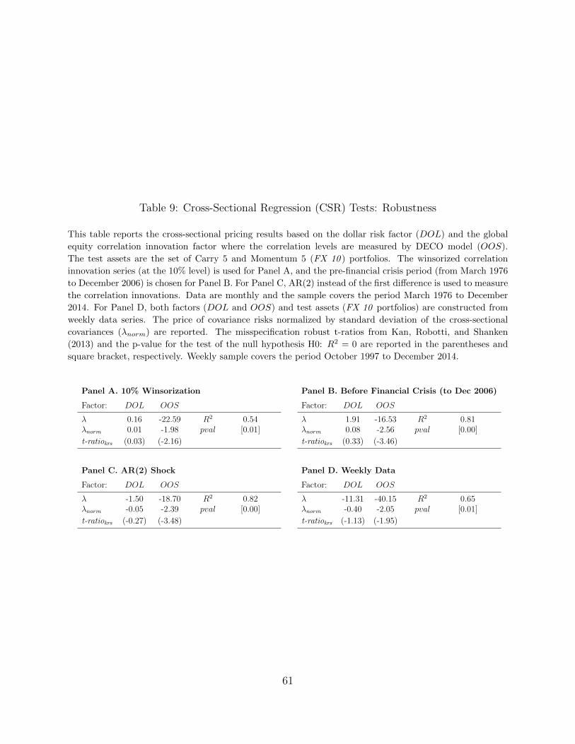
Table 9: Cross-Sectional Regression (CSR) Tests: Robustness

This table reports the cross-sectional pricing results based on the dollar risk factor (DOL) and the global

equity correlation innovation factor where the correlation levels are measured by DECO model (OOS).

The test assets are the set of Carry 5 and Momentum 5 (FX 10 ) portfolios. The winsorized correlation

innovation series (at the 10% level) is used for Panel A, and the pre-financial crisis period (from March 1976

to December 2006) is chosen for Panel B. For Panel C, AR(2) instead of the first difference is used to measure

the correlation innovations. Data are monthly and the sample covers the period March 1976 to December

2014. For Panel D, both factors (DOL and OOS) and test assets (FX 10 portfolios) are constructed from

weekly data series. The price of covariance risks normalized by standard deviation of the cross-sectional

covariances (λnorm) are reported. The misspecification robust t-ratios from Kan, Robotti, and Shanken

(2013) and the p-value for the test of the null hypothesis H0: R2 = 0 are reported in the parentheses and

square bracket, respectively. Weekly sample covers the period October 1997 to December 2014.

Panel A. 10% Winsorization Panel B. Before Financial Crisis (to Dec 2006)

Factor: DOL OOS Factor: DOL OOS

λ 0.16 -22.59 R2 0.54 λ 1.91 -16.53 R2 0.81λnorm 0.01 -1.98 pval [0.01] λnorm 0.08 -2.56 pval [0.00]

t-ratiokrs (0.03) (-2.16) t-ratiokrs (0.33) (-3.46)

Panel C. AR(2) Shock Panel D. Weekly Data

Factor: DOL OOS Factor: DOL OOS

λ -1.50 -18.70 R2 0.82 λ -11.31 -40.15 R2 0.65λnorm -0.05 -2.39 pval [0.00] λnorm -0.40 -2.05 pval [0.01]

t-ratiokrs (-0.27) (-3.48) t-ratiokrs (-1.13) (-1.95)

61

Table 10: Parameter Choices and Moments of Simulated Carry and Momentum Portfolios

We simulate the consumption dynamics of 200 countries, and drive the changes in spot rates and excessreturns of the corresponding currencies through Equation 5 and 6. We choose our parameters followingMenzly, Santos, and Veronesi (2004) and Christoffersen, Du, and Elkamhi (2015), and our choice of param-eters are presented in Panel A. To be consistent with our empirical analysis, we create five carry portfoliossorted on interest differentials and five momentum portfolios sorted on the past three month excess returns.Moments of excess returns of the simulated carry and momentum portfolios are presented in Panel B.

Panel A

A.1. Consumption Dynamicsg σ

0.02 0.015

A.2. Volatility Dynamicsαw θw βw σw,t=0

0.07 1.30 0.80 0.01

A.3. Correlation Dynamicsκρ ρ αρ ρi,t=0

0.01 0.30 180 0.30

A.4. Risk Aversion and SDFκγ γ αγ γi,t=0

0.16 33.9 39.4 20 0.90

Panel B

B.1 Carry Portfolios B.2 Momentum Portfolios

Low 2 3 4 High HML Low 2 3 4 High HML

Mean -2.01 0.50 1.35 1.62 2.27 4.27 -0.90 1.06 1.19 1.68 1.17 2.06Median 0.97 2.23 1.97 1.21 1.78 5.64 -0.31 1.25 0.83 2.74 3.04 2.45Std. Dev 18.47 12.54 11.24 10.64 10.70 16.58 15.29 11.56 11.17 11.15 12.52 10.88Skewness -0.08 -0.02 -0.02 0.07 0.11 0.10 -0.01 0.02 0.02 0.06 -0.09 -0.30Kurtosis 3.90 3.71 4.01 4.23 4.92 5.11 3.44 3.97 4.02 3.97 4.62 5.59Sharpe Ratio -0.11 0.04 0.12 0.15 0.21 0.26 -0.06 0.09 0.11 0.15 0.09 0.18AR(1) -0.06 0.00 -0.02 0.01 -0.03 -0.03 -0.08 -0.04 0.02 0.03 0.03 -0.08

62

Table A1: Country Selection

CountryFX All FX DM

Equity DM

(1973 ~)

Equity

(1988 ~)

Equity

(1995 ~)

Number of country 44 17 17 31 39

1.Australia V V V V V

2.Austria V V V V V

3.Belgium V V V V V

4.Brazil V V V

5.Bulgaria

6.Canada V V V V V

7.Croatia V

8.Cyprus V

9.Czech Repulbic V V

10.Denmark V V V V V

11.Egypt V V

12.Euro area V V

13.Finland V V V

14.France V V V V V

15.Germany V V V V V

16.Greece V V V

17.Hong Kong V V

18.Hungary V V

19.Iceland V

20.India V V

21.Indonesia V V V

22.Ireland V V V

23.Israel V V

24.Italy V V V V V

25.Japan V V V V V

26.Kuwait

27.Malaysia V V V

28.Mexico V V V

29.Netherlands V V V V V

30.New Zealand V V V V V

31.Norway V V V V V

32.Philippines V V V

33.Poland V V

34.Portugal V V V

35.Russia V V

36.Saudi Arabia

37.Singapore V V V

38.Slovakia V

39.Slovenia V

40.South Africa V V

41.South Korea V V V

42.Spain V V V V V

43.Sweden V V V V V

44.Switzerland V V V V V

45.Taiwan V V V

46.Thailand V V V

47.Ukraine V

48.UK V V V V V

49.US V V V

FX Equity

63