Global climate response to anthropogenic aerosol indirect effects: Present...

ClickHere

for

FullArticle

Global climate response to anthropogenic aerosol indirect effects:Present day and year 2100

Wei‐Ting Chen,1,2 Athanasios Nenes,3 Hong Liao,4 Peter J. Adams,5 Jui‐Lin F. Li,1,2

and John H. Seinfeld6

Received 12 December 2008; revised 6 January 2010; accepted 7 January 2010; published 26 June 2010.

[1] Aerosol indirect effects (AIE) are a principal source of uncertainty in future climatepredictions. The present study investigates the equilibrium response of the climate systemto present‐day and future AIE using the general circulation model (GCM), GoddardInstitute for Space Studies (GISS) III. A diagnostic formulation correlating cloud dropletnumber concentration (Nc) with concentrations of aerosol soluble ions is developed as abasis for the calculation. Explicit dependence on Nc is introduced in the treatments ofliquid‐phase stratiform clouds in GISS III. The model is able to reproduce the generalpatterns of present‐day cloud frequency, droplet size, and radiative balance observed byCloudSat, Moderate Resolution Imaging Spectroradiometer, and Earth Radiation BudgetExperiment. For perturbations of Nc from preindustrial to present day, a net AIE forcing of−1.67 W m−2 is estimated, with a global mean surface cooling of 1.12 K, precipitationreduction of 3.36%, a southward shift of the Intertropical Convergence Zone, and ahydrological sensitivity of +3.00% K−1. For estimated perturbations of Nc from present dayto year 2100, a net AIE forcing of −0.58 W m−2, a surface cooling of 0.47 K, and adecrease in precipitation of 1.7% are predicted. Sensitivity calculations show that theassumption of a background minimum Nc value has more significant effects on AIEforcing in the future than on that in present day. When AIE‐related processes are includedin the GCM, a decrease in stratiform precipitation is predicted over future greenhouse gas(GHG)‐induced warming scenario, as opposed to the predicted increase when only GHGand aerosol direct effects are considered.

Citation: Chen, W.‐T., A. Nenes, H. Liao, P. J. Adams, J.‐L. F. Li, and J. H. Seinfeld (2010), Global climate response toanthropogenic aerosol indirect effects: Present day and year 2100, J. Geophys. Res., 115, D12207, doi:10.1029/2008JD011619.

1. Introduction

[2] Aerosols alter the energy balance of the Earth‐atmosphere system directly by scattering and absorbingsunlight (aerosol direct effect (ADE)), and indirectly byaffecting the reflectivity, lifetime, and precipitation forma-tion of clouds. The so‐called aerosol indirect effect (AIE),the modification of cloud optical properties (cloud albedo

effect), structure, and precipitation (cloud lifetime effect) byaerosols, is judged to be the most uncertain radiative forcingin the climate system [Forster et al., 2007]. General circu-lation models (GCMs) with explicit aerosol‐cloud interac-tions are the principal tool for estimating the radiative forcingand climatic impacts of the AIE. Current GCM‐basedestimation of AIE radiative forcing from preindustrial topresent day for the cloud albedo effect range from −0.22 to−1.85 W m−2; when changes in cloud lifetime and otherfeedbacks (e.g., glaciation indirect effects and thermody-namic effects) are included, the values vary from −0.29 to−2.41 W m−2 [Forster et al., 2007].[3] Climatic impacts of the present‐day AIE, relative to

preindustrial conditions, have been investigated in GCMstudies [Rotstayn et al., 2000; Williams et al., 2001;Rotstayn and Lohmann, 2002; Kristjánsson et al., 2005;Ming et al., 2005; Kirkevåg et al., 2008a, 2008b; Koch etal., 2009]. In these studies the atmosphere is coupled to aslab ocean with interactive sea surface temperature (SST)and fixed heat transport. A qualitatively similar pattern inclimate responses was found in these studies: cooling atNorthern Hemisphere high latitudes and a southward dis-placement of the Intertropical Convergence Zone (ITCZ).

1Department of Environmental Science and Engineering, CaliforniaInstitute of Technology, Pasadena, California, USA.

2Now at Jet Propulsion Laboratory, California Institute of Technology,Pasadena, California, USA.

3Schools of Earth and Atmospheric Sciences and Chemical andBiomolecular Engineering, Georgia Institute of Technology, Atlanta,Georgia, USA.

4LAPC, Institute of Atmospheric Physics, Chinese Academy of Sciences,Beijing, China.

5Departments of Civil and Environmental Engineering and Engineeringand Public Policy, Carnegie Mellon University, Pittsburgh, Pennsylvania, USA.

6Departments of Environmental Science and Engineering and ChemicalEngineering, California Institute of Technology, Pasadena, California,USA.

Copyright 2010 by the American Geophysical Union.0148‐0227/10/2008JD011619

JOURNAL OF GEOPHYSICAL RESEARCH, VOL. 115, D12207, doi:10.1029/2008JD011619, 2010

D12207 1 of 23

http://dx.doi.org/10.1029/2008JD011619

Amplified cooling at northern high latitudes associated withsea ice and snow albedo feedbacks was identified byWilliams et al. [2001] and Kristjánsson et al. [2005]. Instudies exploring the combined impacts of present‐dayaerosol direct and indirect effects [Feichter et al., 2004;Kristjánsson et al., 2005; Takemura et al., 2005; Kirkevåg etal., 2008a, 2008b; Koch et al., 2009], a weakening of thehydrological cycle over northern high latitudes and a similarsouthward shift of ITCZ was diagnosed. Combining thedirect and indirect aerosol climatic effects with greenhousegas (GHG) forcing, Feichter et al. [2004] identified a sig-nificant nonlinearity in the response of the hydrologicalcycle using the ECHAM4 model with interactive sulfurchemistry and primary carbonaceous aerosols, and onlinecloud droplet activation. However, in a similar study usingthe CCM‐Oslo (based on the NCAR Community ClimateModel CCM3) with online sulfate and black carbon andlookup tables for CCN activation, Kirkevåg et al. [2008a]found the climatic responses to aerosols and GHG arenearly additive.[4] In the present work, climate responses to the AIE are

studied, with emphasis on changes in the hydrological cycle.We address the following questions: (1) How is climateaffected by the anthropogenic perturbations of cloud dropletnumber concentration (Nc) alone from preindustrial topresent day (year 2000), and from present day to future

(year 2100)? (2) How is future climate predicted to beinfluenced by the combined perturbations of anthropogenicGHG, aerosols, and Nc?[5] Here we use equilibrium climate simulations to

investigate the above questions. The simulations are per-formed using the Goddard Institute for Space Studies(GISS) Global Climate Middle Atmosphere Model III(referred to as GISS III hereafter) coupled to a slab (Q‐flux)ocean model. Modifications are made to the formulations ofoptical depth and autoconversion rates in liquid‐phasestratiform clouds in GISS III to introduce explicit depen-dence on grid‐by‐grid offline Nc fields. In each of the si-mulations, specific levels of offline monthly averagedaerosol mass concentrations and Nc values are input, and theatmospheric dynamics, hydrological cycle, and temperatureare allowed to respond accordingly. The correspondingaerosol indirect radiative forcing is calculated, and changesin cloud properties, temperature, precipitation, and circula-tion between the equilibrium climates are diagnosed. Notethat the aerosol indirect effects on stratiform ice clouds andconvective clouds are not included in the present study.[6] A key ingredient in representing the AIE in GCMs is

the relation of changes in aerosol amount and properties tochanges in Nc and cloud droplet size distribution. In theempirical diagnostic approach, Nc is formulated as a func-tion of aerosol mass or number concentration, based onambient data [e.g., Boucher and Lohmann, 1995; Ghan etal., 1997; Menon et al., 2002; Dufresne et al., 2005; Minget al., 2005; Quaas and Boucher, 2005]. In the prognosticapproach, the cloud droplet distribution is predicted basedon cloud microphysics [e.g., Kristjánsson et al., 2005;Takemura et al., 2005; Lohmann et al., 2007]. While theearliest studies of the AIE employed the empirical diag-nostic approach, the tendency in recent work is to adopt aprognostic microphysics approach to predict cloud dropletproperties online and interactively. In the present study, weestablish a new, physically based, computationally efficientformulation to relate aerosols and cloud properties diag-nostically, allowing for geographical and seasonal variationsof aerosol‐cloud interactions.[7] In section 2, a description of the diagnostic aerosol‐

cloud formulation is provided, together with the derivationsof offline aerosol mass concentrations and offline Nc values,as well as the modifications to the cloud scheme in the GISSIII GCM. The associated forcing for perturbations of GHGand aerosols direct and indirect effects is reported in section 3.Experimental design of the equilibrium climate simulationsis outlined in section 4, with the results of the simulationsanalyzed and discussed in section 5.

2. Descriptions of Global Models

[8] Three different global models were used in this study:the Unified Model developed in the National Aeronauticsand Space Administration (NASA) project “Chemistry,Aerosols, and Climate: Tropospheric Unified Simulation”(termed the “CACTUS Unified Model” hereafter), the Two‐Moment Aerosol Sectional microphysics model withinGoddard Institute for Space Studies (GISS) GCM II′ (GISS‐TOMAS hereafter), and the GISS III GCM. Table 1 sum-marizes the characteristics of each model, its usage here, and

Figure 1. Schematic diagram for experimental design.

CHEN ET AL.: AEROSOL INDIRECT CLIMATIC EFFECTS D12207D12207

2 of 23

relevant references. Figure 1 is a flowchart of the simulationsin this study, and the steps in which each model is involved.First, the CACTUSUnifiedModel is used, with fully coupledsimulations of tropospheric chemistry, aerosols, and cli-mate, to calculate an annual cycle of monthly averagedaerosol mass concentrations for preindustrial (PI, roughlycorresponding to the year 1800), year 2000 (20C), and year2100 (21C). Next, grid‐by‐grid correlation formulationsbetween Nc and aerosol soluble ions are developed usingGISS‐TOMAS and the sectional cloud condensation nuclei(CCN) activation parameterization of Nenes and Seinfeld[2003] (hereafter NS) with the droplet growth kinetic mod-ifications of Fountoukis and Nenes [2005] (hereafter FN).With this formulation and the aerosol mass concentrationsfrom the CACTUSUnifiedModel, offline, monthly averagedvalues of Nc for PI, 20C, and 21C are calculated. Finally,optical depth and autoconversion rates in the liquid‐phasestratiform cloud scheme of GISS III are adjusted to includeexplicit dependence on Nc. A set of equilibrium climate si-mulations was carried out, each with specific levels of GHG,offline aerosol mass, and offline Nc. The differences betweenthe equilibrium simulations were analyzed to identify theimpacts of AIE on the hydrological cycle and future climatechanges.

2.1. CACTUS Unified Model and Offline Aerosol MassConcentration

[9] The CACTUSUnifiedModel, based on the 4°‐latitude‐by‐5°‐longitude, 9 layer GISS GCM II′, simulates the fullycoupled interactions of chemistry, aerosol, and climate [Liaoet al., 2003; 2004; Liao and Seinfeld, 2005]. The model iscoupled to a Q‐flux ocean, with monthly horizontal heattransport fluxes taken fromMickley et al. [2004]. Changes inthe sea surface temperature and sea ice are determined byenergy exchange with the atmosphere, ocean heat transport,and the ocean mixed layer heat capacity [Hansen et al.,

1984; Russell et al., 1985]. The model includes detailedtropospheric O3‐NOx‐hydrocarbon chemistry, as well asheterogeneous processes, such as hydrolysis of N2O5 andirreversible absorption of NO3, NO2, and HO2 on wettedparticle surfaces. Aerosol species predicted in the modelinclude sulfate, nitrate, ammonium, black carbon (BC), pri-mary (POA) and secondary organic aerosol (SOA), sea salt,and mineral dust. Condensation and dry and wet deposition(not size‐dependent) are included in determining the aerosolmass budgets. The CACTUS Unified Model has been used ina number of climate studies to identify the influence of cli-mate change on the predictions of tropospheric chemistry andaerosol [Liao et al., 2006], the climatic impact of ADE [Chenet al., 2007], and the differences between fully coupled andoffline chemistry‐aerosol‐climate simulations [Liao et al.,2009].[10] In the version of the CACTUS Unified Model used

here, the formation of SOA from monoterpenes is based onexperimentally determined yield parameters [Griffin et al.,1999a, 1999b; Chung and Seinfeld, 2002], assuming equi-librium partitioning; SOA formation from isoprene is notincluded in the current version of the model, which will beupdated in future work. The aerosol semidirect effect onclouds (i.e., through changes in the atmospheric temperaturestructure caused by aerosol absorption), in‐cloud chemistry,and wet removal of aerosols are accounted for. The modeldoes not include the climatic impact of AIE on the predic-tion of aerosol fields. On the basis of the calculations givenby Liao et al. [2006], a 10% increase in global meanprecipitation results in a 9–13% decrease in burdens oftracer‐like aerosols (e.g., BC and POA). Since the globalprecipitation change owing to AIE is generally less than2%, as shown later in the climate simulations, the effectsof neglecting AIE‐induced climate change on global meanpredicted aerosol mass in the present study should besmall, but we note that some regional biases may exist.

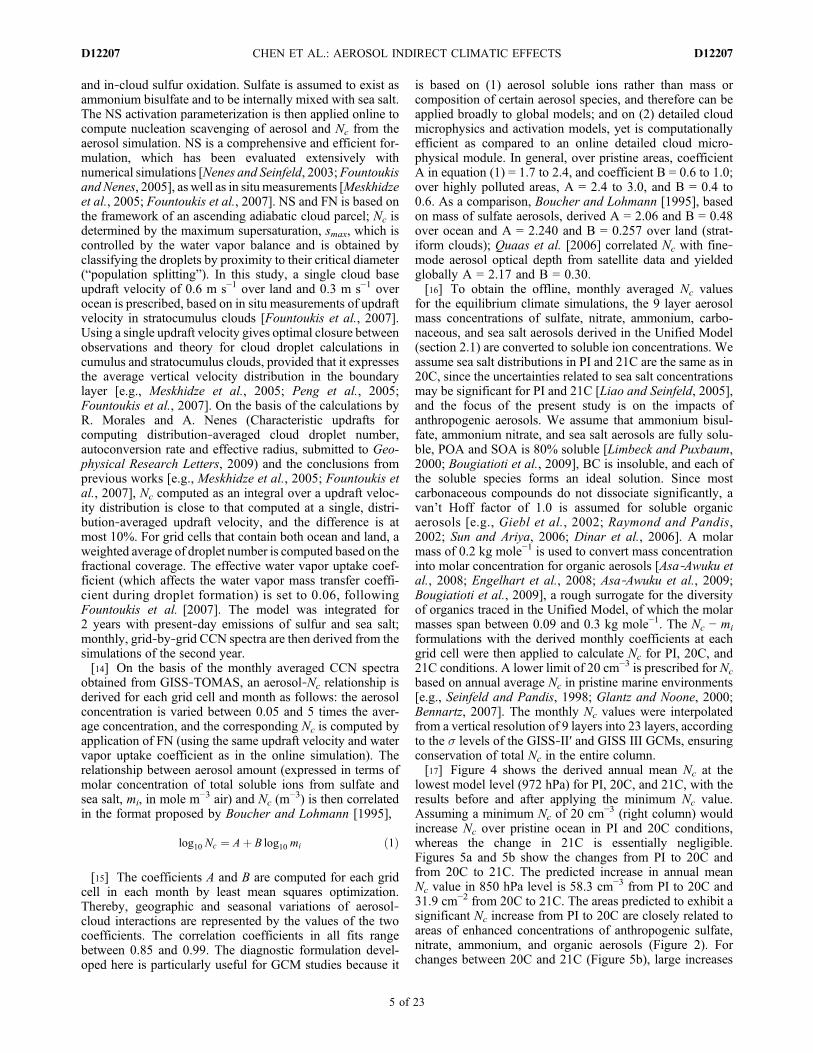
Table 1. Global Models in This Studya

ModelHorizontalResolution s‐Layers

ModelTop (hPa) Feature

Simulations Performedin This Study Reference

CACTUS unifiedmodel

4° Lat by 5° Lon 9 10 Fully coupled chemistry‐aerosol‐climate simulations

Derivation of offlineaerosol concentrations

Liao et al. [2003, 2004] andLiao and Seinfeld [2005]

GISS‐TOMAS 4° Lat by 5° Lon 9 10 Size‐resolved aerosol andCCN concentrations

Calculation of CCNspectra for deriving Nc

aerosol correlations

Adams and Seinfeld,[2002] and Pierce and

Adams [2006]GISS III 4° Lat by 5° Lon 23 0.002 Cloud scheme modified to include

first and second AIEEquilibrium climate

simulationRind et al. [2007]

aAIE, Aerosol indirect effects; GISS, Goddard Institute for Space Studies; CCN, cloud condensation nuclei.

Table 2. Global Annual Burdens of Aerosols Derived by the CACTUS Unified Modela

PI Year 2000 (20C) Year 2100 (21C)

Global NH SH Global NH SH Global NH SH

Ammonium bisulfate 0.41 0.19 0.22 2.87 2.27 0.60 2.74 2.01 0.73Ammonium nitrate 0.22 0.11 0.11 0.67 0.48 0.19 2.88 2.44 0.44POA 0.08 0.05 0.03 1.23 0.88 0.35 2.88 2.11 0.77SOA 0.17 0.08 0.09 0.28 0.18 0.10 0.38 0.26 0.12BC 0.01 0.006 0.004 0.23 0.18 0.05 0.52 0.42 0.10(Total) 0.89 0.44 0.45 5.28 3.99 1.29 9.40 7.24 2.16Sea salta ‐ ‐ ‐ 4.96 1.64 3.32 ‐ ‐ ‐

aPresent‐day (20C) sea salt concentrations are used in the calculation of preindustrial (PI) and 21C Nc fields. Units are Tg dry mass. POA, primaryorganic aerosol; SOA, secondary organic aerosol; BC, black carbon. NH, Northern Hemisphere; SH, Southern Hemisphere.


3 of 23

[11] Three simulations with the CACTUS Unified Modelwere carried out, each using emissions of aerosols, aerosolprecursors, and ozone precursors corresponding to PI, 20C,and 21C, while GHG were held at present‐day levels in allthe simulations. Emissions for 20C and 21C are based onIntergovermental Panel on Climate Change (IPCC) SpecialReport on Emissions Scenarios (SRES) A2. Emissions forPI are based on those for 20C, with relevant scaling (asdetailed by Liao and Seinfeld [2005] and Liao et al. [2006]).All three simulations were initiated by an equilibrium cli-mate corresponding to 20C GHG and integrated for 6 years.Since the levels of GHG are fixed throughout the simula-tions, the differences between the derived PI, 20C and 21Caerosol concentrations result entirely from emission changes.Results from the last 5 years in each simulation are averagedto obtain a grid‐by‐grid, annual cycle of monthly averagedaerosol mass concentrations. These aerosol concentrationsare used later in deriving the offline Nc values (section 2.2)

and also to account for aerosol direct radiative effects (ADE)in the climate simulations (section 2.3.3).[12] Table 2 lists the predicted global and hemispheric

annual burdens of ammonium bisulfate, ammonium nitrate,POA, SOA, BC, and sea salt aerosols, derived for PI, 20C,and 21C. Each of the above species shows significantincrease from PI to 20C. From 20C to 21C, sulfates arepredicted to decrease owing to reductions in projected SO2

emissions; nitrate levels are predicted to increase more thanfourfold, while POA and BC are predicted to double.Figure 2 shows the annual global mean column burdens ofanthropogenic aerosol for PI, 20C, and 21C. Increases inpeak concentrations are predicted over heavily industrial-ized and populated areas of South and East Asia, Europe,and the eastern United States. Outflows from the majorbiomass burning regions in South America and westernAfrica are also prominent. Predicted global column bur-dens of sea salt for 20C are shown in Figure 3. With apredicted global burden of 4.96 Tg, sea salt concentrationsare highest over the southern ocean and the midlatitudeocean over Northern Hemisphere (NH), corresponding tothe strong winds that lead to high emissions in these areas.

2.2. GISS‐TOMAS Model, FN ActivationParameterization, and Derivation of Aerosol‐Nc

Relationships

[13] GISS‐TOMAS and the NS activation parameteriza-tion (with the mass transfer corrections as implemented inFN) are used to provide the diagnostic relationship betweenaerosol levels and Nc. The size‐resolved TOMAS micro-physics module simulates aerosol number concentration,size distribution, composition, and CCN online within theGISS GCM II′; detailed descriptions are provided by Adamsand Seinfeld [2002] for sulfate simulations and Pierce andAdams [2006] for the implementation of sea salt aerosol.In brief, the module tracks both the number and the mass ofaerosols in each size bin in the aerosol distribution. A sec-tional approach is applied to define the boundaries of 30 sizebins (spanning approximately dry diameters of 0.01 to 10 mm),in terms of dry aerosol mass. Microphysical processesinclude coagulation, condensation/evaporation, nucleation,

Figure 2. Annual mean total column burden (mg m−2) ofsulfate, nitrate, ammonium, primary organic aerosol(POA), secondary organic aerosol (SOA), and black carbon(BC) for (a) preindustrial (PI), (b) 20th century (20C), and(c) 21st century (21C). Global average values are given inthe upper right corner of each plot.

Figure 3. Annual mean column burden of sea salt (mg m−2)for 20C. Global average values are given in the upper rightcorner.


4 of 23

and in‐cloud sulfur oxidation. Sulfate is assumed to exist asammonium bisulfate and to be internally mixed with sea salt.The NS activation parameterization is then applied online tocompute nucleation scavenging of aerosol and Nc from theaerosol simulation. NS is a comprehensive and efficient for-mulation, which has been evaluated extensively withnumerical simulations [Nenes and Seinfeld, 2003;Fountoukisand Nenes, 2005], as well as in situmeasurements [Meskhidzeet al., 2005; Fountoukis et al., 2007]. NS and FN is based onthe framework of an ascending adiabatic cloud parcel; Nc isdetermined by the maximum supersaturation, smax, which iscontrolled by the water vapor balance and is obtained byclassifying the droplets by proximity to their critical diameter(“population splitting”). In this study, a single cloud baseupdraft velocity of 0.6 m s−1 over land and 0.3 m s−1 overocean is prescribed, based on in situ measurements of updraftvelocity in stratocumulus clouds [Fountoukis et al., 2007].Using a single updraft velocity gives optimal closure betweenobservations and theory for cloud droplet calculations incumulus and stratocumulus clouds, provided that it expressesthe average vertical velocity distribution in the boundarylayer [e.g., Meskhidze et al., 2005; Peng et al., 2005;Fountoukis et al., 2007]. On the basis of the calculations byR. Morales and A. Nenes (Characteristic updrafts forcomputing distribution‐averaged cloud droplet number,autoconversion rate and effective radius, submitted to Geo-physical Research Letters, 2009) and the conclusions fromprevious works [e.g., Meskhidze et al., 2005; Fountoukis etal., 2007], Nc computed as an integral over a updraft veloc-ity distribution is close to that computed at a single, distri-bution‐averaged updraft velocity, and the difference is atmost 10%. For grid cells that contain both ocean and land, aweighted average of droplet number is computed based on thefractional coverage. The effective water vapor uptake coef-ficient (which affects the water vapor mass transfer coeffi-cient during droplet formation) is set to 0.06, followingFountoukis et al. [2007]. The model was integrated for2 years with present‐day emissions of sulfur and sea salt;monthly, grid‐by‐grid CCN spectra are then derived from thesimulations of the second year.[14] On the basis of the monthly averaged CCN spectra

obtained from GISS‐TOMAS, an aerosol‐Nc relationship isderived for each grid cell and month as follows: the aerosolconcentration is varied between 0.05 and 5 times the aver-age concentration, and the corresponding Nc is computed byapplication of FN (using the same updraft velocity and watervapor uptake coefficient as in the online simulation). Therelationship between aerosol amount (expressed in terms ofmolar concentration of total soluble ions from sulfate andsea salt, mi, in mole m−3 air) and Nc (m

−3) is then correlatedin the format proposed by Boucher and Lohmann [1995],

log10 Nc ¼ Aþ B log10 mi ð1Þ

[15] The coefficients A and B are computed for each gridcell in each month by least mean squares optimization.Thereby, geographic and seasonal variations of aerosol‐cloud interactions are represented by the values of the twocoefficients. The correlation coefficients in all fits rangebetween 0.85 and 0.99. The diagnostic formulation devel-oped here is particularly useful for GCM studies because it

is based on (1) aerosol soluble ions rather than mass orcomposition of certain aerosol species, and therefore can beapplied broadly to global models; and on (2) detailed cloudmicrophysics and activation models, yet is computationallyefficient as compared to an online detailed cloud micro-physical module. In general, over pristine areas, coefficientA in equation (1) = 1.7 to 2.4, and coefficient B = 0.6 to 1.0;over highly polluted areas, A = 2.4 to 3.0, and B = 0.4 to0.6. As a comparison, Boucher and Lohmann [1995], basedon mass of sulfate aerosols, derived A = 2.06 and B = 0.48over ocean and A = 2.240 and B = 0.257 over land (strat-iform clouds); Quaas et al. [2006] correlated Nc with fine‐mode aerosol optical depth from satellite data and yieldedglobally A = 2.17 and B = 0.30.[16] To obtain the offline, monthly averaged Nc values

for the equilibrium climate simulations, the 9 layer aerosolmass concentrations of sulfate, nitrate, ammonium, carbo-naceous, and sea salt aerosols derived in the Unified Model(section 2.1) are converted to soluble ion concentrations. Weassume sea salt distributions in PI and 21C are the same as in20C, since the uncertainties related to sea salt concentrationsmay be significant for PI and 21C [Liao and Seinfeld, 2005],and the focus of the present study is on the impacts ofanthropogenic aerosols. We assume that ammonium bisul-fate, ammonium nitrate, and sea salt aerosols are fully solu-ble, POA and SOA is 80% soluble [Limbeck and Puxbaum,2000; Bougiatioti et al., 2009], BC is insoluble, and each ofthe soluble species forms an ideal solution. Since mostcarbonaceous compounds do not dissociate significantly, avan’t Hoff factor of 1.0 is assumed for soluble organicaerosols [e.g., Giebl et al., 2002; Raymond and Pandis,2002; Sun and Ariya, 2006; Dinar et al., 2006]. A molarmass of 0.2 kg mole−1 is used to convert mass concentrationinto molar concentration for organic aerosols [Asa‐Awuku etal., 2008; Engelhart et al., 2008; Asa‐Awuku et al., 2009;Bougiatioti et al., 2009], a rough surrogate for the diversityof organics traced in the Unified Model, of which the molarmasses span between 0.09 and 0.3 kg mole−1. The Nc − mi

formulations with the derived monthly coefficients at eachgrid cell were then applied to calculate Nc for PI, 20C, and21C conditions. A lower limit of 20 cm−3 is prescribed for Nc

based on annual average Nc in pristine marine environments[e.g., Seinfeld and Pandis, 1998; Glantz and Noone, 2000;Bennartz, 2007]. The monthly Nc values were interpolatedfrom a vertical resolution of 9 layers into 23 layers, accordingto the s levels of the GISS‐II′ and GISS III GCMs, ensuringconservation of total Nc in the entire column.[17] Figure 4 shows the derived annual mean Nc at the

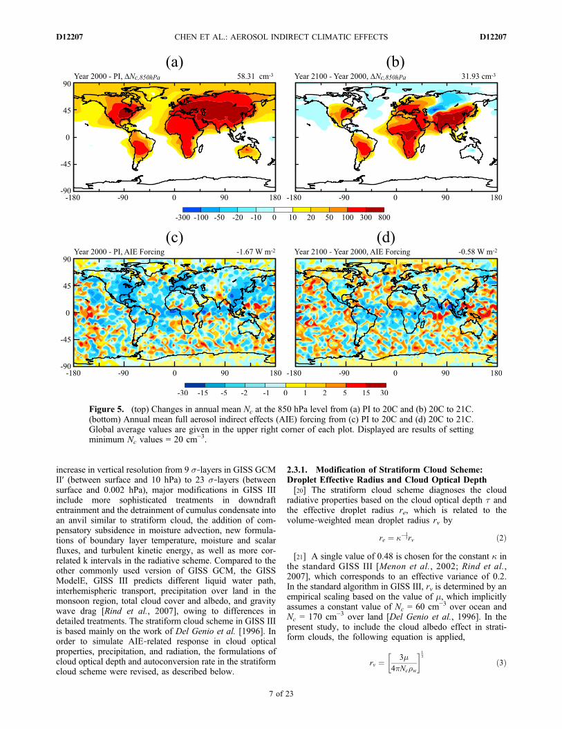
lowest model level (972 hPa) for PI, 20C, and 21C, with theresults before and after applying the minimum Nc value.Assuming a minimum Nc of 20 cm−3 (right column) wouldincrease Nc over pristine ocean in PI and 20C conditions,whereas the change in 21C is essentially negligible.Figures 5a and 5b show the changes from PI to 20C andfrom 20C to 21C. The predicted increase in annual meanNc value in 850 hPa level is 58.3 cm−3 from PI to 20C and31.9 cm−2 from 20C to 21C. The areas predicted to exhibit asignificant Nc increase from PI to 20C are closely related toareas of enhanced concentrations of anthropogenic sulfate,nitrate, ammonium, and organic aerosols (Figure 2). Forchanges between 20C and 21C (Figure 5b), large increases


5 of 23

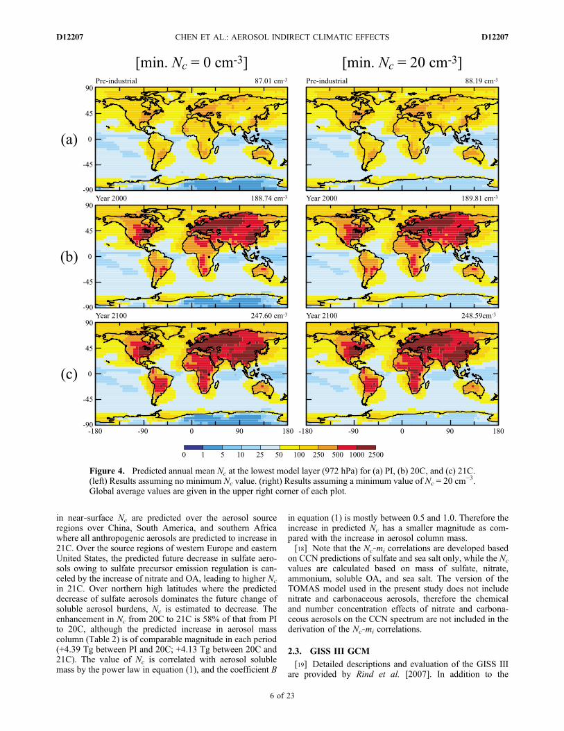
in near‐surface Nc are predicted over the aerosol sourceregions over China, South America, and southern Africawhere all anthropogenic aerosols are predicted to increase in21C. Over the source regions of western Europe and easternUnited States, the predicted future decrease in sulfate aero-sols owing to sulfate precursor emission regulation is can-celed by the increase of nitrate and OA, leading to higher Nc

in 21C. Over northern high latitudes where the predicteddecrease of sulfate aerosols dominates the future change ofsoluble aerosol burdens, Nc is estimated to decrease. Theenhancement in Nc from 20C to 21C is 58% of that from PIto 20C, although the predicted increase in aerosol masscolumn (Table 2) is of comparable magnitude in each period(+4.39 Tg between PI and 20C; +4.13 Tg between 20C and21C). The value of Nc is correlated with aerosol solublemass by the power law in equation (1), and the coefficient B

in equation (1) is mostly between 0.5 and 1.0. Therefore theincrease in predicted Nc has a smaller magnitude as com-pared with the increase in aerosol column mass.[18] Note that the Nc‐mi correlations are developed based

on CCN predictions of sulfate and sea salt only, while the Nc

values are calculated based on mass of sulfate, nitrate,ammonium, soluble OA, and sea salt. The version of theTOMAS model used in the present study does not includenitrate and carbonaceous aerosols, therefore the chemicaland number concentration effects of nitrate and carbona-ceous aerosols on the CCN spectrum are not included in thederivation of the Nc‐mi correlations.

2.3. GISS III GCM

[19] Detailed descriptions and evaluation of the GISS IIIare provided by Rind et al. [2007]. In addition to the

Figure 4. Predicted annual mean Nc at the lowest model layer (972 hPa) for (a) PI, (b) 20C, and (c) 21C.(left) Results assuming no minimum Nc value. (right) Results assuming a minimum value of Nc = 20 cm−3.Global average values are given in the upper right corner of each plot.


6 of 23

increase in vertical resolution from 9 s‐layers in GISS GCMII′ (between surface and 10 hPa) to 23 s‐layers (betweensurface and 0.002 hPa), major modifications in GISS IIIinclude more sophisticated treatments in downdraftentrainment and the detrainment of cumulus condensate intoan anvil similar to stratiform cloud, the addition of com-pensatory subsidence in moisture advection, new formula-tions of boundary layer temperature, moisture and scalarfluxes, and turbulent kinetic energy, as well as more cor-related k intervals in the radiative scheme. Compared to theother commonly used version of GISS GCM, the GISSModelE, GISS III predicts different liquid water path,interhemispheric transport, precipitation over land in themonsoon region, total cloud cover and albedo, and gravitywave drag [Rind et al., 2007], owing to differences indetailed treatments. The stratiform cloud scheme in GISS IIIis based mainly on the work of Del Genio et al. [1996]. Inorder to simulate AIE‐related response in cloud opticalproperties, precipitation, and radiation, the formulations ofcloud optical depth and autoconversion rate in the stratiformcloud scheme were revised, as described below.

2.3.1. Modification of Stratiform Cloud Scheme:Droplet Effective Radius and Cloud Optical Depth[20] The stratiform cloud scheme diagnoses the cloud

radiative properties based on the cloud optical depth t andthe effective droplet radius re, which is related to thevolume‐weighted mean droplet radius rv by

re ¼ ��13rv ð2Þ

[21] A single value of 0.48 is chosen for the constant � inthe standard GISS III [Menon et al., 2002; Rind et al.,2007], which corresponds to an effective variance of 0.2.In the standard algorithm in GISS III, rv is determined by anempirical scaling based on the value of m, which implicitlyassumes a constant value of Nc = 60 cm−3 over ocean andNc = 170 cm−3 over land [Del Genio et al., 1996]. In thepresent study, to include the cloud albedo effect in strati-form clouds, the following equation is applied,

rv ¼ 3�

4�Nc�w

� �13

ð3Þ

Figure 5. (top) Changes in annual mean Nc at the 850 hPa level from (a) PI to 20C and (b) 20C to 21C.(bottom) Annual mean full aerosol indirect effects (AIE) forcing from (c) PI to 20C and (d) 20C to 21C.Global average values are given in the upper right corner of each plot. Displayed are results of settingminimum Nc values = 20 cm−3.


7 of 23

so that rv is determined by m and the offline Nc (m−3) values

imported to each grid cell on a monthly basis. Therefore, reand t are controlled by the spatial and seasonal variations ofNc, which are driven by the changes in aerosol mass andaerosol‐cloud interactions. Note that equation (3) is alsoapplied to compute the radius in droplet evaporation. Addi-tional modifications to the scheme of Del Genio et al. [1996]include a change in the value of � (0.67 over land and 0.80over ocean [Martin et al., 1994]) to reflect the broader dis-tributions of terrestrial clouds (with respect to oceanic),constraints on the minimum and maximum values of re (2and 20 mm, respectively), and a constraint of in‐cloud liquidwater content < 3 g m−3. The above modifications are appliedto pure liquid stratiform clouds only (temperature > 4°C overocean, and > −10°C over land); ice stratiform clouds (tem-perature < −40°C), mixed‐phase stratiform clouds, as well asconvective clouds, follow the scheme of Del Genio et al.[1996].2.3.2. Modification of Stratiform Cloud Scheme:Autoconversion Rate[22] The basic autoconversion formulation in GISS III is

related to that given by Sundqvist et al. [1989],

dqldt

��aut

¼ C0ql 1� e� �

�crit

� �4� �8><

>:

9>=>; ð4Þ

where ql is the cloud liquid water mixing ratio, C0 is thelimiting autoconversion rate (s−1), and mcrit is the critical in‐cloud water content for the onset of rapid conversion. Toexplicitly relate ql to Nc, this parameterization is replacedwith that developed by Khairoutdinov and Kogan [2000](KK hereafter), and modified to account for the fractionalcloudiness in each GCM grid cell,

dqldt

��aut

¼ �1350�bqlb

� �2:47N�1:79c ð5Þ

To ensure that the same radiative balance is maintainedbefore and after the replacement of the autoconversionparameterization, a tuning parameter g is used [Hoose et al.,2008]. In the typical ranges of liquid water and Nc, auto-conversion rates calculated by the KK scheme can be 1 to1000 times smaller than those by the Sundquist scheme[Penner et al., 2006; Hsieh et al., 2009]. When im-plementing the KK scheme in GISS III, proper adjustmentto the autoconversion rates is needed to avoid the uninten-tional increase in liquid water path (LWP) and the subse-quent “drift” toward a cooler climate. The value of g isdetermined by minimizing the imbalance of top‐of‐atmo-sphere (TOA) radiation, the same approach adopted byHoose et al. [2008]. Starting from a present‐day equilibriumclimate predicted by the standard GISS III with fixedpresent‐day SST and sea ice (the HadISST1 observed cli-matology for 1993 to 2002 [Rayner et al., 2003]), themodified GCM is integrated for 1 year, with a specific valueof g. The annual mean TOA net radiation is diagnosed. Bytesting various values between 1 and 100, g = 8.0 producesthe closest net TOA radiation balance and thus is chosen.[23] A new Q‐flux field is derived to secure consistency

between the ocean model and the atmospheric model that

has 20C GHG levels and 20C Nc with modified stratiformcloud scheme. This Q‐flux ocean is then used in all AIEequilibrium climate simulations described in section 4.2.3.3. Aerosol Direct Effect in GISS III[24] The sulfate, nitrate, ammonium and carbonaceous

aerosol masses derived by the Unified Model are also to beused in the equilibrium climate simulations to account forthe anthropogenic aerosol direct effect in GISS III. Calcu-lation of the anthropogenic aerosol direct effect followsChen et al. [2007]. The monthly averaged aerosol massconcentrations derived by the CACTUS Unified Model(section 2.1) are interpolated into 23 layers accordingly.Internal mixing of ammonium sulfate, ammonium nitrate,BC, POA, SOA and aerosol associated water is assumed. Astandard gamma size distribution is assumed for the aerosolmixture with a surface area‐weighted dry radius = 0.3 mmand variance = 0.2. The density of the internally mixedaerosol is computed as the mass‐averaged density of waterand dry aerosols. Refractive indices are derived based on avolume‐weighted mixing rule. The refractive index of drynitrate is assumed the same as that of dry sulfate [Toon etal., 1976], while the refractive indices for organic carbon,BC, and water are from d’Almeida et al. [1991] (organiccarbon as “water soluble,” BC as “soot”). Mie theory isapplied to determine extinction efficiency, single‐scatteringalbedo, and asymmetry parameter from a lookup table,which are then supplied to the radiation scheme of the GCMto calculate the aerosol optical depth and the radiationfluxes. The internal mixing assumption yields a relativelyhigh absorption efficiency per unit mass of BC [e.g.,Haywood et al., 1997; Myhre et al., 1998; Jacobson, 2000;Chung and Seinfeld, 2002, 2005].[25] The ADE of sea salt and dust is accounted for by

using the background, present‐day sea salt and dust opticaldepth climatology provided in the standard GISS III. Thissea salt/dust climatology is identical to that in GISS ModelE,[e.g., Schmidt et al., 2006]. All the simulations used the samesea salt and dust ADE, so the climatic effects of these naturalaerosols are removed when the simulations are differentiatedin pairs. The ADE forcing in the present study results solelyfrom the changes in the internal mixture of anthropogenicaerosols (i.e., sulfate, nitrate, ammonium, and carbonaceousparticles) predicted by the Unified Model.

3. Radiative Forcing

3.1. Radiative Forcing of GHG, ADE, and AIE

[26] Table 3 summarizes the radiative forcings of GHG,ADE, and AIE in the present study. For GHG and ADE, theforcings are determined by the instantaneous change in netradiative fluxes at the tropopause (without adjustment instratospheric temperature). The calculations are carried outwith prescribed present‐day SST and sea ice, using parallelcalls of the radiation scheme. Between the present day andyear 2100, the changes in GHG and ADE in the simulationsare estimated to result in forcings of +6.47 W m−2 and+0.12 W m−2, respectively. These values are close to thosereported by Chen et al. [2007] (+6.58 W m−2 for GHG and+0.18Wm−2 for ADE), which were derived using the 9 layerGISS GCM II′with identical offline aerosol fields and similarGHG levels to the present work.


8 of 23

[27] Because AIE involves feedback mechanisms, theconcept of instantaneous radiative forcing cannot be applied,especially when the cloud lifetime effect is considered. TotalAIE radiative forcing has to be determined by diagnosingthe changes in cloud forcing (CF, i.e., all‐sky minus clear‐sky radiative fluxes), allowing at least the cloud water andprecipitation to respond, as described in the IPCC report[Forster et al., 2007].[28] Total AIE radiative forcing is derived by following

the literatures summarized in IPCC AR4 [Denman et al.,2007]. The full AIE forcing calculations in the presentstudies includes three simulations using prescribed present‐day SST and sea ice and the modified stratiform cloudscheme, each with the offline Nc values for PI, 20C, and21C, respectively. The GHG is fixed to levels in 2000 in allthree calculations. Cloud and precipitation are allowed torespond to different Nc values, while most of the tempera-ture response is suppressed with the fixed SST. Therefore,both cloud albedo and lifetime effects are taken intoaccount. The simulations were integrated for 20 years; witha 5 year spin‐up time, the net cloud forcing (CF, i.e., all‐skyminus clear‐sky net radiative fluxes) at TOA over the last 15years were averaged and compared (Table 3 and Figure 5).The predicted global mean full AIE forcing is −1.67 W m−2

for perturbation of Nc from PI to 20C, lying within therange to total AIE forcing reported in the literature (−0.29to −2.41 W m−2) [e.g., Lohmann and Feichter, 2005;Denman et al., 2007; Forster et al., 2007; Kirkevåg et al.,2008b]. The full AIE forcing is −0.58 W m−2 for pertur-bation of Nc from 20C to 21C. This value is larger thanthat predicted by Kristjansson [2002] (−0.02 W m−2),which is based on the IPCC A2 emission scenario from20C to 21C but considered only changes in anthropogenicsulfate and BC aerosols, implying that the future AIEforcing is mainly contributed by the increase in nitrate andorganic aerosols.

3.2. Sensitivity of AIE Forcing to the Lower Limit of Nc

Concentrations

[29] The AIE forcing can be sensitive to the minimum Nc

concentrations assumed in the calculations [Lohmann andFeichter, 2005]. To explore this sensitivity of the AIEforcing in the present study, we repeat the above AIEforcing calculations with a minimum Nc = 10 cm−3 (Table 3;numbers in parenthesis). When the minimum Nc, is reduced,the magnitude of the AIE forcing between PI and 20C ispredicted to be slightly enhanced (2%). Because predicted

Nc fields in pristine regions are below the minimum value(Figure 4) in both PI and 20C conditions, the magnitudes ofCF in PI and 20C decrease almost equally when a smallerminimum Nc value is used. Thus, the AIE forcing, which isthe difference of CF between PI and 20C, only shows alimited change with the value of minimum Nc. However, theenhancement of AIE forcing between 20C and 21C is moresignificant (+12%). The Nc fields in 21C are generally abovethe minimum value. Since the CF in 21C exhibits smallchange and the CF in 20C decreases with smaller minimumNc, the AIE forcing between 20C and 21C is predicted toincrease when the minimum Nc is set to 10 cm−3.[30] As compared to the previous studies, the present

works predicts a weaker sensitivity of present‐day AIEforcing to the lower limit of Nc. For example, Lohmann andFeichter [2005] showed that an increase of minimum Nc

from 10 to 40 cm−3 results in a higher predicted present‐dayAIE forcing from −1.9 to −1.1 W m−2 (72%); Kirkevåg et al.[2008b] found that a global increase in Nc by 15 cm−3

changes the present‐day AIE forcing from −2.34 to −1.36 Wm−2 (42%); Hoose et al. [2009] calculated a reduction ofglobal mean shortwave (SW) CF from −1.88 to −0.62 Wm−2

(67%) whenminimumNc is increased from 0 to 40 cm−3. Thissensitivity is associated with the differences in original Nc

values (i.e., before any minimum Nc value is applied)predicted over pristine ocean between PI and present‐dayconditions.

4. Experimental Setup for Equilibrium ClimateSimulations With GISS III GCM

[31] The experimental setups of the equilibrium climatesimulations with GISS III are summarized in Table 4. Thenomenclature of the simulations is as follows: (1) Uppercase letters denote the forcing mechanisms imposed on eachsimulation, with G for greenhouse gas forcing, D for aerosolDirect effect, and I for aerosol Indirect effect; and (2) sub-scripts denote the levels of the forcing agents, with PI for

Table 3. AIE, ADE, and GHG Forcing in the Present Study

20C to PI (W m−2) 21C to 20C (W m−2)

Instantaneous ADE forcing ‐ +0.12Instantaneous GHG forcing ‐ +6.47AIE forcing, fulla −1.67 (−1.70, 2%) −0.58 (−0.65, 12%)

aAIE forcing is derived with prescribed sea surface temperature (SST)and the modified stratiform cloud scheme, allowing full response ofcloud water and precipitation. AIE forcing is defined as the change innet (shortwave + longwave) cloud forcing (i.e., all‐sky minus clear‐skynet radiative fluxes) at top of atmosphere (TOA). Values in parenthesisare the AIE forcing with minimum Nc = 10 cm−3 and the percentagechange relative to the case of minimum Nc = 20 cm−3. ADE, aerosoldirect effect. GHG, greenhouse gas.

Table 4. Experimental Design of the Equilibrium Simulationswith GISS III GCMa

Simulationb GHGc ADEd AIEe Years of Integration

GD20C 20C 20C ‐ 100GD21C 21C 21C ‐ 100GD20CI20C 20C 20C 20C 30GD20CIPI 20C 20C PI 30GD20CI21C 20C 20C 21C 30GD21CI21C 21C 21C 21C 30

aGCM, general circulation model.bIn the abbreviations, upper case letters denote the forcings imposed in

each simulations: G, greenhouse gases; D, aerosol direct effects; I,aerosol indirect effects. The subscripts denote the levels of the forcing:PI, preindustrial; 20C, year 2000; 21C, year 2100. The first twosimulations were carried out with the standard GISS III, while the lastfour simulations were performed with the modified GISS III.

cFor 20C levels, CO2 = 367 ppmv, CH4 = 1668 ppbv, N2O = 315 ppbv,CFC=11 = 260 pptv, and CFC=12 = 520 pptv. For 21C levels, CO2 = 856ppmv, CH4 = 3578 ppbv, N2O = 445 ppbv, CFC‐11 = 44 pptv, and CFC‐12 = 216 pptv.

dFrom offline, monthly imposed aerosols of internally mixed sulfate,nitrate, ammonium, BC, POA, SOA, and water.

eFrom offline, monthly imposed Nc in the calculation of optical depthand autoconversion in warm stratiform clouds.


9 of 23

preindustrial level, 20C for year 2000 level, and 21C foryear 2100 level.[32] GHG forcing is imposed by fixing the concentrations

of CO2, CH4, N2O, CFC‐11, and CFC‐12 at specific levels;the values, based on IPCC SRES A2, are listed in thefootnotes in Table 4. ADE forcing is imposed by the usingthe offline, monthly averaged aerosol mass concentrationsfrom the fully coupled CACTUSUnifiedModel (sections 2.1and 2.3.3). AIE forcing is imposed by using the offline,monthly averaged Nc fields derived from the diagnostic for-mulation and aerosol soluble ion concentrations (section 2.2)to perturb cloud optical depth and liquid water (autoconver-sion). The 12 month, annual cycle of both aerosol mass andNc is repeated throughout the entire integration.[33] The first two simulations were carried out to obtain a

starting climate for the four key simulations. These two runsused the standard version of GISS III coupled with a Q‐fluxocean that is consistent with the atmosphere of 20C GHGlevels and standard stratiform cloud scheme (i.e., withoutdroplet‐dependent cloud optical depth and autoconversion).These two 100 year simulations are (1) GD20C: present‐dayequilibrium climate accounting for GHG and anthropogenicaerosol direct effect at present‐day levels; and (2) GD21C:

year 2100 equilibrium climate accounting for GHG andanthropogenic aerosol direct effect at year 2100 levels.[34] The final year climate from the above simulations is

used as the starting point for the following four AIE equi-librium climate runs. These 30 year simulations used themodified GCM with the droplet‐dependent stratiform cloudsand the consistent Q‐flux ocean mentioned in section 2.3.2:(1) GD20CI20C: present‐day equilibrium climate accountingfor GHG and anthropogenic aerosol direct and indirect ef-fects at present‐day levels (offline Nc values correspondingto present‐day aerosol levels); (2) GD20CIPI: equilibriumclimate accounting for GHG and anthropogenic aerosoldirect effect at present‐day levels and aerosol indirect effectsat preindustrial levels (offline Nc values corresponding topreindustrial aerosol levels); (3) GD20CI21C: equilibriumclimate accounting for GHG and anthropogenic aerosoldirect effect at present‐day levels, and aerosol indirect ef-fects at year 2100 levels (offline Nc values corresponding toyear 2100 aerosol levels); and (4) GD21CI21C: year 2100equilibrium climate accounting for GHG, and anthropogenicaerosol direct and indirect effects at year 2100 levels (offlineNc values corresponding to year 2100 aerosol levels).[35] Statistics over the last 20 years of each of the above

equilibrium climates are determined. Differences betweenthe simulations are analyzed as follows: (1) GD20C versusGD20CI20C: the effect of incorporating explicit droplet‐dependent autoconversion and optical depth and offline Nc

values on present‐day equilibrium climate (section 5.1); (2)GD20CI20C versus GD20CIPI: differences in equilibrium cli-mate owing only to changes in Nc between preindustrial andpresent day (section 5.2); (3) GD20CI21C versus GD20CI20C:differences in equilibrium climate owing only to changesin Nc between present day and year 2100 (section 5.3); and(4) GD21CI21C versus GD20CI20C: differences in equilibriumclimate between present day and year 2100 accounting forchanges in GHG and anthropogenic aerosol direct and indi-rect effects (section 5.4).[36] When differentiating each pair of the simulations, the

two‐sample “usual” t test was applied to calculate the 95%confidence intervals [Zwiers and von Storch, 1995; Chen et

Table 5. Global Annual Mean Values of Key Climate Variablesin the Present‐Day Equilibrium Simulations With and WithoutExplicit Droplet Dependence in Stratiform Clouds

Climate Variablea GD20C GD20CI20C

Ts (°C) 14.52 14.45Total cloud (%) 61.31 61.16Strat. cloud (%) 57.05 56.87Low cloud (%) 51.70 51.30TOA SW cloud forcing (W m−2) −53.41 −53.84LWP (g m−2) 119.38 111.49Precip., (mm d−1) 2.99 2.98Precip. (strat.) (mm d−1) 0.96 0.93Surface SW flux (W m−2) 161.98 162.83

aTs, surface temperature; SW, shortwave flux; CF, cloud forcing; LWP,liquid water path; precip., precipitation; strat., stratiform.

Table 6. Comparison of Global Annual Mean Cloud Properties in Present‐Day SimulationGD20CI20CWith Remote Sensing Observationsand Predictions in Selected GCM Studies

GD20CI20C Observation Modeling Studies

Total column Nca (1010 m−2) 6.16 4.4b 2.1 to 7.6c

Nc at 850 hPa (cm−3) 122.22 ‐ 75.0 to 135.0d

re at cloud tope (mm) (global) 12.18, (land)9.26, (ocean) 13.10

(global) 11.4f and 14.7,g

(land) 12.5,g (ocean) 15.6g(global) 6.8 to 11.3h

LWP (g m−2) 111.49 93.3i 41.5 to 110.0j

TOA SW CF (W m−2) −53.84 −50.0k −49.9 to −61.0l

aAccounts for cloudy periods in cloudy regions only.bHan et al. [1998] (International Satellite Cloud Climatology Project (ISCCP), average of January, April, July, and October 1987).cMenon et al. [2002] (GISS II with prescribed SST) and Hoose et al. [2008] (ECHAM5‐HAM with in‐cloud aerosol processing scheme and prescribed

SST).dPenner et al. [2006] (CAM‐Oslo, LMD‐Z, and CCSR with prescribed SST, in exp. 6).eModeled values are multiplied by 21/3 to approximate cloud top condition in the satellite retrievals.fHan et al. [1994] (ISCCP, average of January, April, July, and October 1987).gMeskhidze et al. [2007] (Moderate Resolution Imaging Spectroradiometer (MODIS), 2000 to 2006).hMenon et al. [2002], Kristjánsson et al. [2005] (CCM‐Oslo with slab ocean, exp. ALLTOT), and Penner et al. [2006].iPenner et al. [2006] (MODIS).jKristjánsson et al. [2005], Penner et al. [2006], and Hoose et al. [2008].kKiehl and Trenberth [1997] (Earth Radiation Budget Experiment (ERBE), November 1984 through February 1990).lCollins et al. [2006a] (CCSM3), Collins et al. [2006b] (CAM3), Penner et al. [2006], Hoose et al. [2008], and Kirkevåg et al. [2008b] (CAM‐Oslo).


10 of 23

al., 2007] (see Table 7, footnote). The results reported insections 4 and 5 are statistically significant, unless otherwiseexplicitly noted.

5. Responses of the Equilibrium Climate

5.1. Predicted Present‐Day Equilibrium Climate

[37] Comparing simulations GD20C versus GD20CI20C, itis found that (Table 5) replacement of the autoconversionscheme results in a smaller (−4.1%) global annual meanLWP, which can be explained as follows. The offline,present‐day Nc values imposed on the modified model are,on average, higher than the constant values of Nc implicitlyassumed in the standard model in the calculation of cloud

optical depth (section 2.3.1). Before replacing and tuningthe autoconversion scheme, this change in Nc fields alonecauses the predicted stratiform clouds to be more reflective(results not shown). Since the new autoconversion scheme istuned to match the overall TOA radiation balance simulatedin the standard model (section 2.3.2), to compensate for theprevious effect of higher Nc, the tuning eventually results ina lower LWP in the modified model. The modified GISS IIIalso predicts a slightly cooler global mean surface temper-ature (4.45 K versus 4.52 K), less cloud cover, stronger(more negative) SW CF, and a more positive surface SWflux, whereas the predicted global mean precipitation rate isessentially identical between the standard and modifiedversions of GISS III.[38] Several key cloud properties in the predicted present‐

day equilibrium climate with AIE‐related processes(GD20CI20C) are compared to satellite‐retrieved climatologyin Table 6 and Figures 6–8; the remote sensing instruments,observational periods, and related references are given in thefootnotes for Table 6 and captions for Figures 6–8. Note that

Figure 6. Zonal vertical distribution of present‐day cloudfrequency from (top) CloudSat observations (from July2001 to August 2002) and (bottom) Goddard Institute forSpace Studies (GISS) III general circulation model (GCM)prediction (GD20CI20C, accounting for aerosol indirect effects).

Figure 7. Present‐day cloud droplet radius at warm cloudtop from (top) Moderate Resolution Imaging Spectroradi-ometer (MODIS) retrievals (year 2000 to 2006) and (bottom)GISS III GCM prediction (GD20CI20C, accounting for aerosolindirect effects). Global average values are given in the upperright corner of each plot.


11 of 23

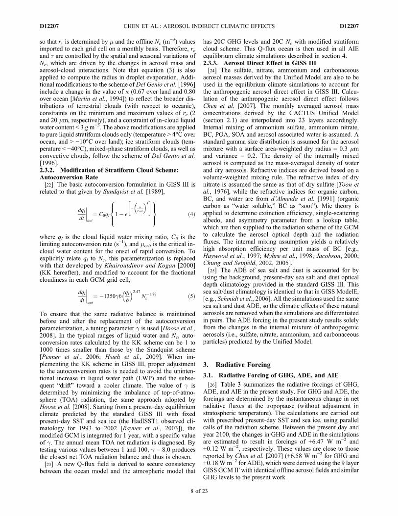
exact agreement is not expected because of different timeperiods as well as the fact that the simulation is an equi-librium climate corresponding to present‐day forcing,whereas the data reflect the actual transient climate. Also,the model data are sampled and summed at each time step(i.e., every 1 h for cloud microphysics; every 4 h for radiativeproperties), more frequently than the sampling of the satelliteretrievals. Thus, the general latitudinal distributions of thevariables are most relevant.[39] Figure 6 compares the modeled present‐day annual

mean total cloud frequency zonal vertical profile (inGD20CI20C) with observation from the CloudSat cloud pro-filing radar (version 5.1, release 4 [RO4], August 2006 toJuly 2007). CloudSat measures the backscattered powerusing a 94 GHz, nadir‐viewing radar to derive cloud andprecipitation properties [Stephens et al., 2008]. The modi-fied GISS III captures the general shape of the cloud fre-quency zonal vertical distribution, including the ITCZ overthe tropics and the midlatitude storm tracks. For low‐levelliquid cloud, which is the focus in the present study, thealtitude of peak cloud frequency at midlatitudes in GISS IIIlocates around 950–900 hPa (the second and third modellayers), lower than the peak altitude at 850 hPa in theCloudSat observation (corresponding to the fourth modellayer in GISS III). GISS III also overestimates the low cloudnear the Tropics. The cloud frequency predicted in thestandard GISS III (GD20C) is essentially identical to that inthe modified model (not shown), implying the biases are notrelated to the modifications of the stratiform cloud scheme.The lower altitude of midlatitude liquid cloud frequency andoverestimation of Tropical shallow clouds are commonlypredicted in many GCMs (results not shown). These dif-ferences between the modeled and observed low‐level cloudfrequency may be related to the facts that (1) vertical reso-lution is different between GISS III (increasing from 200 min the first layer to 600 m in the fourth layer) and CloudSat(250 m), (2) low cloud with tops below 1 km (∼900 hPa) areunderrepresented in the CloudSat data, owing to radarclutter contamination from the surface [Stephens et al.,2008], and (3) the uncertainties in cloud parameterization,

such as the relative humidity (RH) threshold for determiningcloudiness in the RH‐based stratiform cloud scheme inGISS GCM.[40] Figure 7 compares the predicted global annual mean

re at warm cloud top in GD20CI20C with the climatologyretrieved by Moderate Resolution Imaging Spectro-radiometer (MODIS Terra, Collection 005, Level‐3, quality‐assured pixel‐weighted cloud properties averaged at 1° by1° resolution; composites were made using monthly averagesof available MODIS data from year 2000 to 2006 [Meskhidzeet al., 2007; M. King et al., Collection 005 change summaryfor the MODIS cloud optical property (06‐OD) algorithm,2006, available at http://modis‐atmos.gsfc.nasa.gov/pro-ducts, C005update.html]) To ensure proper comparison withthe satellite data, the predicted values at cloud top are takenand averaged over cloudy regions with cloud top temperaturehigher than 273 K, with the cloud top defined as the highestGCM layer with liquid water content (LWC) > 10‐9 g m−3

[Meskhidze et al., 2007]. Note that the re in satellite retrievalrepresents the characteristic value at the cloud top, while themodel value represents the average over the entire GCMlayer in which the cloud top resides [Boucher and Lohmann,1995; Quaas et al., 2004; Chen and Penner, 2005;Meskhidze et al., 2007]. To address this issue, we follow thetreatment of Meskhidze et al. [2007] and multiply the mod-eled re at cloud top by 2

1/3, assuming that LWCvaries linearlywith height (i.e., LWC at the top = 2xLWC averaged overthe layer) and Nc remains constant with height in the cloudtop layer. This scaling to the modeled re is applied here onlyfor the comparison with satellite retrievals, but not in theclimate simulations. As compared to MODIS data, GISS IIIsimulates similar land‐ocean contrast of re, with highestvalues over tropical Pacific owing to the conditions of lowNc and high LWC, and lowest values over industrializedregions in China, western Europe and eastern United Statesowing to highly enhanced Nc. However, GISS III system-atically underestimates re by 2 to 3 mm in both land andocean areas, as summarized in Table 6. Such biases arecommon in many present GCMs [Boucher and Lohmann,1995; Quaas et al., 2004; Chen and Penner, 2005;Meskhidze et al., 2007], and are likely related to the un-certainties in the updraft velocity, liquid water content andits variability, and the cloud parameterization in the model,as well as the coarse model resolution and uncertainties inthe retrieval algorithms.[41] Figure 8 shows the zonal mean present‐day short-

wave and longwave TOA cloud forcing. While the predictedlongwave (LW) CF matches well the observations of theEarth Radiation Budget Experiment (ERBE) [Kiehl andTrenberth, 1997], the model‐derived SW CF exhibits anegative bias over the Tropics and a positive bias in mid-latitudes to high latitudes in both hemispheres. Present‐daycloud forcings predicted by modified GISS III (GD20CI20C,black solid lines) are very similar to those in the standardGISS III (GD20C, black dashed lines), indicating the bias inCF is not associated with the AIE‐related processes intro-duced in section 2.3.[42] Table 6 lists the corresponding global mean values

reported in several modeling studies focusing on AIE. Pre-dictions of Nc, re, and CF in simulation GD20CI20C generallyfall within the range of previous studies. Although LWP isoverestimated in the present work when compared to both

Figure 8. Zonal annual mean distribution of present‐daytop‐of‐atmosphere (TOA) shortwave (SW) and longwave(LW) cloud forcing (CF) observations from Earth RadiationBudget Experiment (ERBE) [Kiehl and Trenberth, 1997](gray lines) and predicted in GISS III with AIE process(GD20CI20C, black solid lines) and without AIE process(GD20C, black dashed lines).


12 of 23

Figure 9. Present‐day climate response to perturbation of AIE from preindustrial to present day(GD20CI20C − GD20CIPI): vertical zonal profiles of changes in annual mean (a) Nc in liquid stratiformclouds (cm−3), (b) total cloud water mixing ratio (10−6 kg H2O (kg air) −1), (c) re in liquid stratiformclouds (mm), (d) temperature (K), (e) specific humidity (10−4 kg H2O (kg air) −1), and (f) mass streamfunction (1010 kg s−1; positive values indicate counterclockwise flows); and annual mean changes in(g) Ts (K) and (h) precipitation (mm d−1). Changes that are insignificant relative to the 95% confidenceintervals are shaded. Global average values are given in the upper right corner of Figures 9g and 9h.


13 of 23

observation and previous predictions, one should note theuncertainties involved in the retrieval of this variable, thedifference in cloud schemes and aerosol treatments used invarious global models. Besides, from the simulations dis-cussed subsequently, we find that the LWP in the GISS III issensitive to temperature change, and increased/decreasedLWP is always predicted when the model climate iswarmed/cooled. The high bias of the present‐day LWP can

be explained partly by the fact that the simulated equilibriumclimate is about 0.5 K warmer than the actual present‐dayclimate [Jones et al., 1999], with the “warming commitment”of the GHG forcing not yet fully realized.

5.2. Effects of Change of Nc from Preindustrialto Present Day on Equilibrium Climate

[43] In this section, the equilibrium climate response tothe AIE perturbation from preindustrial to present dayis analyzed, by comparing simulations GD20CI20C andGD20CIPI. In both simulations, the GHG and ADE forcingare fixed at the present‐day level, while offline Nc fieldsfor preindustrial and present‐day conditions are imposed,respectively, in each simulation. The changes in key cli-mate variables (GD20CI20C − GD20CIPI) are summarized inFigures 9 and 10 and the first column in Tables 7 and 8.[44] The maximum increase of Nc in liquid stratiform

clouds (+100 to +400 cm−3) is predicted to occur over 30–60°N, from the surface to 700 hPa, as shown in the latitude‐pressure profile in Figure 9a. The latitudinal distribution ofchanges in Nc at 850 hPa in Figure 10a reveals that theestimated increase in Nc is more pronounced in June–July–August (JJA, dotted line), and located at higher latitudes,than the increase in December–January–February (DJF,gray solid line). Over the region of maximal Nc increase,autoconversion rates are predicted to decrease, which leadsto increased liquid cloud water mixing ratio (+1 to +3 ppmm)in the low and midtroposphere in NH, as shown in Figure 9b.For the change in droplet size, the effect of larger Nc

dominates that of increased cloud water, as the predicted rein warm stratiform cloud decreases by more than 1 mm(Figure 9c). Around 400 hPa over the Tropics, the clouddroplet size is predicted to increase (Figure 9c, 0.2–1.5 mm),owing to the higher cloud water in stratiform clouds (notshown) and the relatively small change in Nc estimated overthis region. Note that pure liquid stratiform clouds do notfrequently occur at this altitude over the Tropics, andtherefore the impact of increasing droplet size should besmall. The estimated change in cloud cover is small (<2% ofabsolute amount in all latitudes) for both stratiform andconvective clouds, and therefore is not shown.[45] As a result of increased cloud optical depths associ-

ated with smaller droplet size and higher cloud water inwarm stratiform clouds, negative changes in zonal meanTOA SW CF of up to −5 W m−2 are predicted over 30–60°N(Figure 10b). The negative AIE forcing results in a predictedglobal cooling of −1.12 K at the surface. Figures 9d and 9eshow that the predicted cooling leads to a decrease inatmospheric water vapor. The maximum cooling near thetropical tropopause is a result of vertical temperature con-vective adjustment toward the moist adiabatic lapse rate; thepattern is similar to the simulated global warming owing toincreased GHG [Manabe and Wetherald, 1975], but with anopposite sign. As displayed in Figures 9g and 10c, thesurface temperature is reduced more significantly in NH(−1.46 K) and over land (−1.31 K), with a prominentcooling over the northern middle to high latitudes. Over 30–50°N, the surface cooling is predicted to be more substantialin JJA; this is also the season of maximum Nc increase andnegative AIE forcing, indicating that the cooling is a directresponse to perturbation of Nc. North of 50°N, however, themost significant cooling is estimated to occur in DJF, when

Figure 10. Present‐day climate response to perturbationof AIE from preindustrial to present day (GD20CI20C −GD20CIPI): zonal mean changes in (a) Nc at 850 hPa (cm−3),(b) TOA SW CF (W m−2), (c) Ts (K), and (d) precipitation(mm d−1) (Black solid lines indicate annual average, graylines indicate average over December–January–February(DJF), and dotted lines indicate average over June–July–August (JJA)).


14 of 23

the change in Nc and TOA SW CF is relatively small. Thispattern of predicted temperature response is similar to thosefound in previous studies investigating present‐day AIEimpacts [Rotstayn et al., 2000; Williams et al., 2001;Rotstayn and Lohmann, 2002; Kristjánsson et al., 2005].[46] The amplification and the difference in the seasons of

peak forcing and surface temperature in the northern highlatitudes are likely related to ice‐albedo feedback as well asfeedback mechanisms involving sea ice, ocean‐atmosphereheat exchange, and atmospheric dynamics, as analyzed byWilliams et al. [2001] and Kristjánsson et al. [2005]. Notethat the previous studies have predicted a more prominent

polar amplification, which is likely associated with the dif-ference in sea ice models, and the fact that aerosol con-centrations were predicted interactively in those studies.However, considering the uncertainties in predicted sea iceand insufficient knowledge of the radiative impact of polarstratiform clouds, the actual mechanism of polar response toAIE requires more detailed studies [Garrett and Zhao,2006].[47] The predicted response in global circulation to sur-

face cooling is a southward displacement of the ITCZ,which manifests itself by the change of distribution of pre-cipitation in Figures 9h and 10d. Figure 9f shows thechanges in zonal mean mass stream function. The moresubstantial cooling in the NH induces a weak anomalousclockwise flow over the Tropics between 20°S and 20°N,but is mostly statistically insignificant. In general, a slowerhydrological cycle is predicted in response to the perturba-tion of Nc from preindustrial to present day. Global annualmean precipitation is predicted to decrease by 0.10 mm d−1

(3.36%), especially in NH (−0.19 mm d−1). The predicteddecrease in stratiform precipitation is only 0.01 mm d−1, andthe precipitation reduction comes mostly from lowerconvective precipitation, owing to decreasing moisture inthe atmosphere. The overall effects of all the feedbackslead to an increase in global mean LWP in stratiform cloud(+1.50 g m−2) but a decrease in total LWP (−4.03 g m−2).The global mean change in TOA net CF is −1.48 W m−2.

Table 7. Changes in Annual Mean Cloud Properties Between theEquilibrium Climatesa

RegionsGD20CI20C −GD20CIPI

GD20CI21C −GD20CI20C


Dcolumn Nc

(1010 m−2)Global +2.96 +1.53 +1.80

Ocean +0.84 +0.28 +0.38Land +9.68 +5.64 +6.18NH +5.37 +2.65 +3.40SH +0.58 +0.49 +0.21

Dre at cloud topb (mm)

Global −0.78 −0.27 (+0.05)

Ocean −0.44 −0.20 +0.03Land −1.84 −0.50 −0.06NH −1.15 −0.31 −0.19SH −0.40 −0.23 +0.20

DLWP (g m−2) Global −4.03 −0.60 +20.45Ocean −4.73 (−0.19) +22.26Land −2.26 −1.66 +15.84NH −6.46 (−1.03) +24.00SH −1.61 (−0.17) +16.89

DLWP (strat.)(g m−2)

Global +1.50 (+0.24) +2.93

Ocean +1.55 +0.42 +2.34Land +1.44 (−0.25) +4.57NH +2.20 (+0.19) +3.77SH +0.79 (+0.27) +2.10

Dstrat. cloud(% (absolute))

Global +0.71 +0.37 −2.00

Ocean +0.61 +0.40 −1.96Land +0.97 (+0.32) −2.08NH +0.63 +0.34 −1.66SH +0.80 +0.41 −2.33

DTOA SW CF(W m−2)

Global −1.61 −0.69 −1.88

Ocean −1.42 −0.88 −1.72Land −2.08 (−0.22) −2.29NH −2.48 −0.94 −2.35SH (−0.74) (−0.44) −1.42

Dnet CF (W m−2) Global −1.48 −0.62 −2.18Ocean −1.13 −0.72 −2.20Land −2.37 −0.39 −2.14NH −2.58 −0.86 −2.34SH (−0.39) (−0.39) −2.03

aDifferences insignificant relative to the 95% confidence intervals areparenthesized. The usual t test takes into account the temporal correlationin each set of sample data (i.e., the global, land, ocean, or hemisphericalannual average of the climate variable of interest in the last 20 years ofeach simulation). The sample sizes are reduced to the equivalent samplesizes ne and me. The 95% confidence interval equals to 1.98 × s × (1/ne+1/me)

0.5 if ne + me ≥ 30, where s is the pooled standard deviation; forne + me < 30, the interval is determined by a lookup table. For a moredetailed explanation, please refer to Zwiers and von Storch [1995].

bValues reported here are not scaled by 21/3 as in the model‐satellitecomparison.

Table 8. Similar to Table 7, but for Changes in Annual MeanTemperature, Precipitation, Hydrological Sensitivity, and SurfaceRadiative Fluxes

RegionsGD20CI20C −GD20CIPI



DTs (K) Global −1.12 −0.47 +4.60Ocean −0.99 −0.43 +4.20Land −1.46 −0.58 +5.61NH −1.31 −0.47 +4.63SH (−0.93) −0.48 +4.58

Dprecip.(mm d−1)

Global −0.10 −0.05 +0.26

Ocean −0.08 −0.04 +0.32Land −0.16 −0.09 +0.12NH −0.19 −0.06 +0.29SH (−0.02) −0.04 +0.23

Dprecip. (strat.)(mm d−1)

Global −0.01 −0.01 −0.01

Ocean −0.01 −0.01 −0.02Land −0.04 −0.02 +0.02NH −0.01 −0.01 −0.03SH (−0.00) −0.01 +0.01

Dprecip./ DTs(% K−1)

Global +3.00 +3.57 +1.90

Dsurface SWflux (W m−2)

Global −2.38 −1.08 +0.91

Ocean −1.90 −1.07 +0.91Land −3.60 −1.12 +0.92NH −2.93 −1.06 +0.44SH −1.83 −1.12 +1.38

Dsurface LWflux (W m−2)

Global −0.84 −0.39 +6.17

Ocean −1.22 −0.53 +7.12Land (+0.12) (−0.04) +3.75NH −1.00 −0.39 +6.02SH −0.68 −0.39 +6.32


15 of 23

Figure 11. Similar to Figure 9 but for present‐day climate response to perturbation of AIE from presentday to year 2100 (GD20CI21C − GD20CI20C).


16 of 23

5.3. Perturbations of Nc from Present Day to Year 2100to Equilibrium Climate

[48] The equilibrium climate response to the AIE pertur-bation from present day to year 2100 is diagnosed here, bycomparing simulations GD20CI21C and GD20CI20C. Present‐day GHG and ADE forcings are used in both simulations,while the imposed Nc values in each simulation are forpresent day and year 2100, respectively. The results(GD20CI21C − GD20CI20C) are presented in Figures 11 and 12and the second column of Tables 7 and 8.[49] In NH, the predicted Nc increase from present day to

year 2100 is smaller than that from preindustrial to presentday, and the interhemispheric contrast is not as great. Over

NH high latitudes, Nc is predicted to slightly decrease (−15to −20 cm−3) in JJA (Figures 11a and 12a), corresponding tothe estimated reduction in sulfate aerosols in this region[Chen et al., 2007]. Also, the latitude of peak increase in Nc

is predicted to shift southward to 30°N. The changes in Nc inthe lower troposphere lead to a slight increase in cloud water(+0.1 to +0.5 ppmm) and a decrease in re in warm stratiformclouds (−0.2 to −0.5 mm) (Figures 11b and 11c). Theresponse in cloud cover is, again, insensitive to the pertur-bation in Nc. The predicted global mean surface cooling is−0.47 K, with small cooling over low and midlatitudes andamplified cooling over the polar regions (Figures 11g and12c). Statistically significant cooling of −0.5 to −1.0 K ispredicted over NH continents in midlatitudes to high lati-tudes. The maximum cooling near the tropical tropopauseassociated with water vapor feedback is still evident.[50] The response in general circulation to the pattern of

predicted surface cooling is mostly insignificant. A similarsouthward displacement of the ITCZ is predicted, leading toa suppression in annual mean precipitation around theequator by as much as 0.4 mm d−1 (Figure 11h and 12d). Thepredicted global mean precipitation reduction from presentday to year 2100 is 0.05 mm d−1 (1.68%). The predictedglobal mean LWP also exhibits a decrease (−0.60 g m−2).

5.4. Combined Effects of GHG, ADE, and AIE FromPresent Day to Year 2100 on Equilibrium Climate

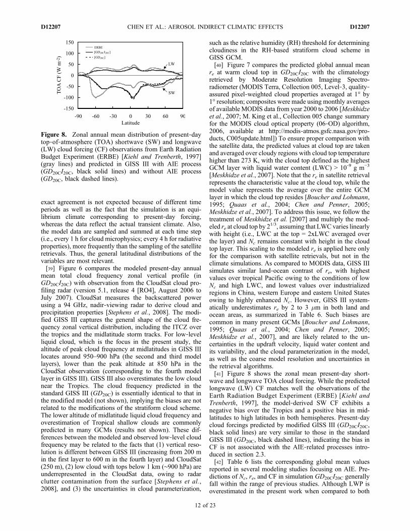
[51] The differences between the equilibrium climates(GD21CI21C − GD20CI20C), revealing the response to thecombined forcing of GHG, ADE, and AIE from present dayto year 2100, are outlined in Figures 13 and 14 and the thirdcolumn of Tables 7 and 8. The changes in Nc are similar tothose in section 4.3 and hence not displayed. As expected,the general pattern of the response is largely dominated bythe GHG‐induced warming. The increase of equilibriumglobal surface temperature from present day to year 2100 ispredicted to be 4.60 K. The warming is prominentlyamplified in polar regions by snow and ice albedo feedbackand near the tropical tropopause through moist adiabaticadjustment (Figures 13a, 13d, and 14a). A broadened andweakened Hadley cell is revealed in the predicted differencein mass stream function (Figure 13c). Global annual meantotal precipitation is predicted to increase by 0.26 mm d−1.The latitudinal pattern of excess precipitation (total precip-itation minus total evaporation) is enhanced (Figure 14b),owing to the effects of increasing water vapor (Figure 13b)and increasing poleward moisture transport (not shown), asdiscussed by Held and Soden [2006]. A poleward shift ofthe storm tracks is also predicted (not shown). The predictedchange in Hadley circulation, excess precipitation, andstorm track, are consistent qualitatively with the projectedfuture climate in most of the IPCC Fourth AssessmentReport (AR4) models in response to GHG induced warming[e.g., Mitas and Clement, 2005; Held and Soden, 2006;Meehl et al., 2007].[52] It is of interest to compare this present day to year

2100 equilibrium climate response to that predicted by thestandard version of GISS III (i.e., [GD21C − GD20C] versus[GD21CI21C − GD20CI20C]). According to Table 9, themodified GISS III, which incorporates AIE‐related strati-form clouds, predicts a slightly weaker warming (4.60 Kversus 4.85 K), less precipitation increase (0.26 mm d−1

Figure 12. Similar to Figure 10 but for present‐day climateresponse to perturbation of AIE from present day to year2100 (GD20CI21C − GD20CI20C).


17 of 23

versus 0.30 mm d−1), and smaller reduction of absolutecloud cover (−2.24% versus −2.38%). The most pronounceddifference between the predicted responses is the reversedsign in the change of stratiform cloud precipitation:−0.01 mm d−1 in the modified GISS III versus +0.05 mm d−1

in the standard GISS III. Figures 14c and 15c show that thestandard model predicts minimal change of stratiformprecipitation over Tropics and subtropics, in contrast to thepredicted decrease of stratiform precipitation of 0.2 to0.3 mm d−1 in the modified model over the same regions.This reveals the impact of the AIE on suppressing stratiformprecipitation. The predicted latitudinal distributions of tem-perature, precipitation, and circulation changes are similar inboth versions (Figures 14 and 15).

5.5. Hydrological Sensitivities

[53] The hydrological sensitivity is defined as the ratio ofthe percentage change in global total precipitation to theglobal surface temperature change. This section comparesthe hydrological sensitivity of AIE from 20C to 21C esti-mated in the current study with those reported in two relatedstudies, Chen et al. [2007] and Liao et al. [2009] (Table 10),and in the literature. Chen et al. [2007] simulated theequilibrium climate response to ADE and GHG frompresent day to year 2100, based on SRES A2 scenario,using the 9 layer GISS II′ GCM. The 20C and 21C offlineaerosol fields used in that study are very similar to those inthe present work (before interpolation from 9 to 23 ver-tical layers). Liao et al. [2009] performed fully coupled

Figure 13. Climate responses to combined effects of greenhouse gas (GHG) and anthropogenic aerosoldirect and indirect effects from present day to year 2100 (GD21CI21C − GD20CI20C): vertical zonal profilesof changes in annual mean (a) temperature (K), (b) specific humidity (10−4 kg H2O (kg air) −1), and (c)mass stream function (1010 kg s−1); annual mean changes in (d) Ts (K) and (e) precipitation (mm d−1).Global average values are given in the upper right corner of Figures 13d and 13e. Note the colorscales are different from those of previous figures.


18 of 23

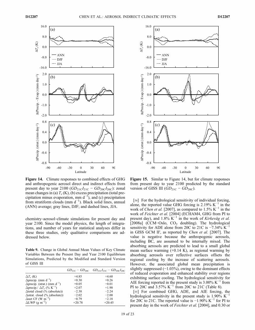
chemistry‐aerosol‐climate simulations for present day andyear 2100. Since the model physics, the length of integra-tions, and number of years for statistical analyses differ inthese three studies, only qualitative comparisons are ad-dressed below.

[54] For the hydrological sensitivity of individual forcing,alone, the reported value GHG forcing is 2.19% K−1 in thework of Chen et al. [2007], as compared to 1.5% K−1 in thework of Feichter et al. [2004] (ECHAM4, GHG from PI topresent day), and 1.8% K−1 in the work of Kirkevåg et al.[2008a] (CCM−Oslo, CO2 doubling). The hydrologicalsensitivity for ADE alone from 20C to 21C is −7.34% K−1

in GISS GCM II′, as reported by Chen et al. [2007]. Thevalue is negative because the anthropogenic aerosols,including BC, are assumed to be internally mixed. Theabsorbing aerosols are predicted to lead to a small globalmean surface warming (+0.14 K), as regional warming byabsorbing aerosols over reflective surfaces offsets theregional cooling by the increase of scattering aerosols.However, the associated global mean precipitation isslightly suppressed (−1.03%), owing to the dominant effectsof reduced evaporation and enhanced stability over regionsexhibiting surface cooling. The hydrological sensitivity forAIE forcing reported in the present study is 3.00% K−1 fromPI to 20C and 3.57% K−1 from 20C to 21C (Table 8).[55] For combined GHG, ADE, and AIE forcing, the

hydrological sensitivity in the present study is 1.90% K−1

for 20C to 21C. The reported value is −1.90% K−1 for PI topresent day in the work of Feichter et al. [2004], and 0.30 or

Figure 14. Climate responses to combined effects of GHGand anthropogenic aerosol direct and indirect effects frompresent day to year 2100 (GD21CI21C − GD20CI20C): zonalmean changes in (a) Ts (K), (b) excess precipitation (total pre-cipitation minus evaporation, mm d−1), and (c) precipitationfrom stratiform clouds (mm d−1). Black solid lines, annual(ANN) average; gray lines, DJF; and dashed lines, JJA.

Table 9. Change in Global Annual Mean Values of Key ClimateVariables Between the Present Day and Year 2100 EquilibriumSimulations, Predicted by the Modified and Standard Versionof GISS III

GD21C − GD20C GD21CI21C − GD20CI20C

DTs (K) +4.85 +4.60Dprecip. (mm d−1) +0.30 +0.26Dprecip. (strat.) (mm d−1) +0.05 −0.01Dprecip./ DTs (% K−1) +2.07 +1.90Dtotal cloud (% (absolute)) −2.38 −2.24Dstrat. cloud (% (absolute)) −2.02 −2.00Dnet CF (W m−2) −0.79 −2.18DLWP (g m−2) +20.78 +20.45

Figure 15. Similar to Figure 14, but for climate responsesfrom present day to year 2100 predicted by the standardversion of GISS III (GD21C − GD20C).


19 of 23

0.24% K−1 for a combined 2XCO2 and changed aerosolemissions from PI to present day or year 2100, respectively,in the work of Kirkevåg et al. [2008a]. In the multimodelensemble average in the IPCC 2007 report [Meehl et al.,2007], considering transient response to GHG and allother forcings with the A2 scenario from 20C to 21C, thehydrological sensitivity is 1.45% K−1. These very differentvalues indicate high uncertainties associated with thehydrological processes in the model when the effects ofaerosols and GHG are included simultaneously. Note thatFeichter et al. [2004] and Kirkevåg et al. [2008a] bothsimulated full aerosol‐cloud‐climate interactions. Thehydrological sensitivity may be highly sensitive to thedegree of “coupling” in the model. For example, Liao et al.[2009] calculated the fully coupled response to ADE andGHG changes from 20C to 21C with the GISS GCM II′ andderived a hydrological sensitivity of 1.5% K−1, smaller thanthat for GHG with offline ADE in the standard GISS III inthe present study (2.07% K−1).

6. Summary and Conclusions

[56] To investigate the climatic impacts of aerosol indirecteffects with GISS III GCM, explicit dependence on Nc hasbeen introduced to the formulations of optical depth andautoconversion rates for liquid stratiform clouds in theGCM, to account for both cloud albedo and lifetime effects.Fully coupled chemistry‐aerosol‐climate simulations withthe CACTUS Unified Model have been carried out to obtainoffline aerosol mass concentrations. Additionally, using si-mulations with the GISS‐TOMAS microphysics model and

the FN CCN activation parameterization, grid‐by‐grid cor-relations between aerosol soluble ion concentration and Nc

have been established. The diagnostic correlations havebeen applied to the aerosol mass predicted in the UnifiedModel to compute corresponding offline Nc fields.[57] Two 100 year simulations using the standard GISS III

have been carried out, each with GHG and aerosol directforcing from offline aerosol mass for present day or year2100, to provide starting climates for the four equilibriumclimate simulations using the GISS III with AIE‐relatedimplementation, each integrated for 30 years. By imposingoffline monthly averaged Nc for PI, present day, and year2100 in each simulation, the climate responses to the per-turbations of Nc have been analyzed. The general patternsof the climate responses are summarized below and inTable 11.[58] The perturbation of Nc from PI to 20C, of which the

full AIE forcing is −1.67 W m−2, is predicted to cause anequilibrium global surface cooling of 1.12 K, with maxi-mum cooling at the NH high latitudes. The predictedinterhemispheric temperature gradient induces an anoma-lous general flow between 20°S and 20°N, and a southwarddisplacement of the ITCZ. The equilibrium global meanprecipitation reduction is 0.10 mm d−1, with a correspondinghydrological sensitivity of 3.00% K−1. The results are con-sistent with previous GCM studies on preindustrial topresent‐day AIE forcing.[59] The perturbation of Nc from 20C to 21C, which is

weaker in magnitude and has different latitudinal distribu-tion than that from PI to 20C, results in a full AIE forcingof −0.58 W m−2. A small decrease of 0.47 K in predicted

Table 10. Comparisons of Present Day to Year 2100 Hydrological Sensitivity Between the Present Study and Two Previous RelatedStudies

Types of Forcing GHG ADE GHG + ADE GHG + ADE AIE GHG + ADE + AIE

Study Chen et al.[2007]

Chen et al.[2007]

Liao et al. [2009] Present study Present study Present study

GCM GISS II′ GISS II′ CACTUS unifiedmodel (GISS II′)

StandardGISS III

ModifiedGISS III

ModifiedGISS III

Predictions of aerosols and/orNc in the simulations

— Offline Online with fullycoupled chemistry

and climate

Offline Offline Offline

Integration (diagnostic period) (years) 80 (last 30) 80 (last 30) 35 (last 20) 100 (last 20) 100+30 (last 20) 100+30 (last 20)Equilibrium response of global Ts (K) +5.31 +0.14 +6.00 +4.85 −0.47 +4.60Equilibrium response of global precip. (%) +11.64 −1.03 +9.00 +10.03 −1.68 +8.72Hydrological sensitivity (% K−1) +2.19 −7.34 +1.5 +2.07 +3.57 +1.90

Table 11. Summary of Patterns of Equilibrium Climate Response in the Present Studya

Perturbation of Nc From PI to 20C Perturbation of Nc From 20C to 21CPerturbation of GHG, ADE and Nc

From 20C to 21C

Change in Nc Increase globally with maximaover 30–60°N

Maximum of increase over 15–45°N;slight decrease north of 60°N in JJA

Maximum of increase over 15–45°N;slight decrease north of 60°N in JJA

Surface temperature Cooling globally, with amplificationespecially at NH high lat.

Small cooling over the Tropics andsubtropics; polar amplified

Warming globally with polar amplification

General circulation Weak clockwise flow over theTropics; southward shift of ITCZ

Weak clockwise flow over the Tropics;southward shift of ITCZ

Broadened Hadley Cell; strengthenedascending branches in convection zone

Precipitation Reduced global average; maximumdecrease over the Tropics; slightly

enhanced around 15°S

Slightly reduced global average;maximum decrease over the Tropics;

Enhanced global average with maximumat Equator; decreased stratiformprecipitation over 45°S to 45°N

aJJA, June–July–August.


20 of 23

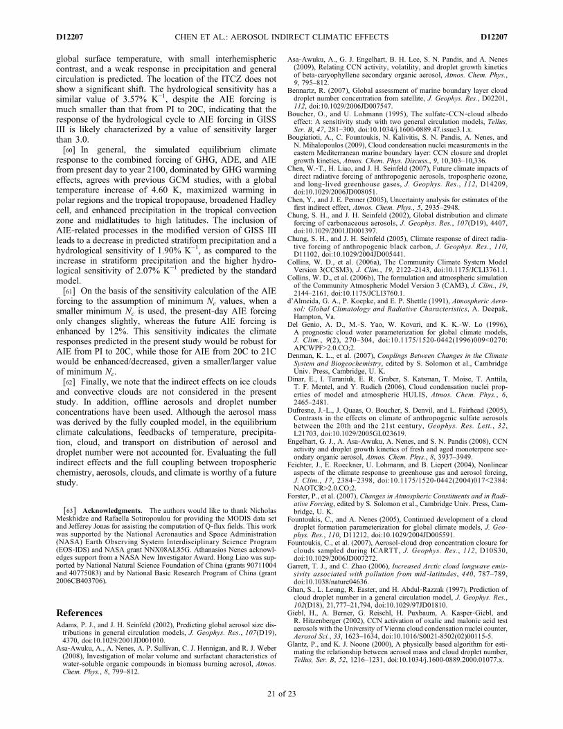
global surface temperature, with small interhemisphericcontrast, and a weak response in precipitation and generalcirculation is predicted. The location of the ITCZ does notshow a significant shift. The hydrological sensitivity has asimilar value of 3.57% K−1, despite the AIE forcing ismuch smaller than that from PI to 20C, indicating that theresponse of the hydrological cycle to AIE forcing in GISSIII is likely characterized by a value of sensitivity largerthan 3.0.[60] In general, the simulated equilibrium climate

response to the combined forcing of GHG, ADE, and AIEfrom present day to year 2100, dominated by GHG warmingeffects, agrees with previous GCM studies, with a globaltemperature increase of 4.60 K, maximized warming inpolar regions and the tropical tropopause, broadened Hadleycell, and enhanced precipitation in the tropical convectionzone and midlatitudes to high latitudes. The inclusion ofAIE‐related processes in the modified version of GISS IIIleads to a decrease in predicted stratiform precipitation and ahydrological sensitivity of 1.90% K−1, as compared to theincrease in stratiform precipitation and the higher hydro-logical sensitivity of 2.07% K−1 predicted by the standardmodel.[61] On the basis of the sensitivity calculation of the AIE

forcing to the assumption of minimum Nc values, when asmaller minimum Nc is used, the present‐day AIE forcingonly changes slightly, whereas the future AIE forcing isenhanced by 12%. This sensitivity indicates the climateresponses predicted in the present study would be robust forAIE from PI to 20C, while those for AIE from 20C to 21Cwould be enhanced/decreased, given a smaller/larger valueof minimum Nc.[62] Finally, we note that the indirect effects on ice clouds

and convective clouds are not considered in the presentstudy. In addition, offline aerosols and droplet numberconcentrations have been used. Although the aerosol masswas derived by the fully coupled model, in the equilibriumclimate calculations, feedbacks of temperature, precipita-tion, cloud, and transport on distribution of aerosol anddroplet number were not accounted for. Evaluating the fullindirect effects and the full coupling between troposphericchemistry, aerosols, clouds, and climate is worthy of a futurestudy.

[63] Acknowledgments. The authors would like to thank NicholasMeskhidze and Rafaella Sotiropoulou for providing the MODIS data setand Jefferey Jonas for assisting the computation of Q‐flux fields. This workwas supported by the National Aeronautics and Space Administration(NASA) Earth Observing System Interdisciplinary Science Program(EOS‐IDS) and NASA grant NNX08AL85G. Athanasios Nenes acknowl-edges support from a NASA New Investigator Award. Hong Liao was sup-ported by National Natural Science Foundation of China (grants 90711004and 40775083) and by National Basic Research Program of China (grant2006CB403706).

ReferencesAdams, P. J., and J. H. Seinfeld (2002), Predicting global aerosol size dis-tributions in general circulation models, J. Geophys. Res., 107(D19),4370, doi:10.1029/2001JD001010.

Asa‐Awuku, A., A. Nenes, A. P. Sullivan, C. J. Hennigan, and R. J. Weber(2008), Investigation of molar volume and surfactant characteristics ofwater‐soluble organic compounds in biomass burning aerosol, Atmos.Chem. Phys., 8, 799–812.

Asa‐Awuku, A., G. J. Engelhart, B. H. Lee, S. N. Pandis, and A. Nenes(2009), Relating CCN activity, volatility, and droplet growth kineticsof beta‐caryophyllene secondary organic aerosol, Atmos. Chem. Phys.,9, 795–812.

Bennartz, R. (2007), Global assessment of marine boundary layer clouddroplet number concentration from satellite, J. Geophys. Res., D02201,112, doi:10.1029/2006JD007547.

Boucher, O., and U. Lohmann (1995), The sulfate‐CCN‐cloud albedoeffect: A sensitivity study with two general circulation models, Tellus,Ser. B, 47, 281–300, doi:10.1034/j.1600-0889.47.issue3.1.x.

Bougiatioti, A., C. Fountoukis, N. Kalivitis, S. N. Pandis, A. Nenes, andN. Mihalopoulos (2009), Cloud condensation nuclei measurements in theeastern Mediterranean marine boundary layer: CCN closure and dropletgrowth kinetics, Atmos. Chem. Phys. Discuss., 9, 10,303–10,336.

Chen, W.‐T., H. Liao, and J. H. Seinfeld (2007), Future climate impacts ofdirect radiative forcing of anthropogenic aerosols, tropospheric ozone,and long‐lived greenhouse gases, J. Geophys. Res., 112, D14209,doi:10.1029/2006JD008051.

Chen, Y., and J. E. Penner (2005), Uncertainty analysis for estimates of thefirst indirect effect, Atmos. Chem. Phys., 5, 2935–2948.

Chung, S. H., and J. H. Seinfeld (2002), Global distribution and climateforcing of carbonaceous aerosols, J. Geophys. Res., 107(D19), 4407,doi:10.1029/2001JD001397.

Chung, S. H., and J. H. Seinfeld (2005), Climate response of direct radia-tive forcing of anthropogenic black carbon, J. Geophys. Res., 110,D11102, doi:10.1029/2004JD005441.

Collins, W. D., et al. (2006a), The Community Climate System ModelVersion 3(CCSM3), J. Clim., 19, 2122–2143, doi:10.1175/JCLI3761.1.

Collins, W. D., et al. (2006b), The formulation and atmospheric simulationof the Community Atmospheric Model Version 3 (CAM3), J. Clim., 19,2144–2161, doi:10.1175/JCLI3760.1.

d’Almeida, G. A., P. Koepke, and E. P. Shettle (1991), Atmospheric Aero-sol: Global Climatology and Radiative Characteristics, A. Deepak,Hampton, Va.

Del Genio, A. D., M.‐S. Yao, W. Kovari, and K. K.‐W. Lo (1996),A prognostic cloud water parameterization for global climate models,J. Clim., 9(2), 270–304, doi:10.1175/1520-0442(1996)009<0270:APCWPF>2.0.CO;2.

Denman, K. L., et al. (2007), Couplings Between Changes in the ClimateSystem and Biogeochemistry, edited by S. Solomon et al., CambridgeUniv. Press, Cambridge, U. K.

Dinar, E., I. Taraniuk, E. R. Graber, S. Katsman, T. Moise, T. Anttila,T. F. Mentel, and Y. Rudich (2006), Cloud condensation nuclei prop-erties of model and atmospheric HULIS, Atmos. Chem. Phys., 6,2465–2481.

Dufresne, J.‐L., J. Quaas, O. Boucher, S. Denvil, and L. Fairhead (2005),Contrasts in the effects on climate of anthropogenic sulfate aerosolsbetween the 20th and the 21st century, Geophys. Res. Lett., 32,L21703, doi:10.1029/2005GL023619.

Engelhart, G. J., A. Asa‐Awuku, A. Nenes, and S. N. Pandis (2008), CCNactivity and droplet growth kinetics of fresh and aged monoterpene sec-ondary organic aerosol, Atmos. Chem. Phys., 8, 3937–3949.

Feichter, J., E. Roeckner, U. Lohmann, and B. Liepert (2004), Nonlinearaspects of the climate response to greenhouse gas and aerosol forcing,J. Clim., 17, 2384–2398, doi:10.1175/1520-0442(2004)017<2384:NAOTCR>2.0.CO;2.

Forster, P., et al. (2007), Changes in Atmospheric Constituents and in Radi-ative Forcing, edited by S. Solomon et al., Cambridge Univ. Press, Cam-bridge, U. K.

Fountoukis, C., and A. Nenes (2005), Continued development of a clouddroplet formation parameterization for global climate models, J. Geo-phys. Res., 110, D11212, doi:10.1029/2004JD005591.

Fountoukis, C., et al. (2007), Aerosol‐cloud drop concentration closure forclouds sampled during ICARTT, J. Geophys. Res., 112, D10S30,doi:10.1029/2006JD007272.

Garrett, T. J., and C. Zhao (2006), Increased Arctic cloud longwave emis-sivity associated with pollution from mid‐latitudes, 440, 787–789,doi:10.1038/nature04636.

Ghan, S., L. Leung, R. Easter, and H. Abdul‐Razzak (1997), Prediction ofcloud droplet number in a general circulation model, J. Geophys. Res.,102(D18), 21,777–21,794, doi:10.1029/97JD01810.

Giebl, H., A. Berner, G. Reischl, H. Puxbaum, A. Kasper‐Giebl, andR. Hitzenberger (2002), CCN activation of oxalic and malonic acid testaerosols with the University of Vienna cloud condensation nuclei counter,Aerosol Sci., 33, 1623–1634, doi:10.1016/S0021-8502(02)00115-5.

Glantz, P., and K. J. Noone (2000), A physically based algorithm for esti-mating the relationship between aerosol mass and cloud droplet number,Tellus, Ser. B, 52, 1216–1231, doi:10.1034/j.1600-0889.2000.01077.x.


21 of 23

Griffin, R. J., D. R. Cocker, R. C. Flagan, and J. H. Seinfeld (1999a),Organic aerosol formation from the oxidation of biogenic hydrocarbons,J. Geophys. Res., 104(D3), 3555–3567, doi:10.1029/1998JD100049.

Griffin, R. J., D. R. Cocker, J. H. Seinfeld, and D. Dabdub (1999b), Esti-mate of global atmospheric organic aerosol from oxidation of biogenichydrocarbons, Geophys. Res. Lett., 26(17), 2721–2724, doi:10.1029/1999GL900476.

Han, Q., W. B. Rossow, and A. A. Lacis (1994), Near‐global survey ofeffective droplet radii using ISCCP data, J. Clim., 7, 465–497,doi:10.1175/1520-0442(1994)007<0465:NGSOED>2.0.CO;2.

Han, Q., W. B. Rossow, J. Chou, and R. M. Welch (1998), Global variationof column droplet concentration in low‐level clouds, Geophys. Res. Lett.,25, 1419–1422, doi:10.1029/98GL01095.

Hansen, J., A. Lacis, G. Russel, P. Stone, I. Fung, R. Ruedy, and J. Lerner(1984), Climate sensitivity: Analysis of feedback mechanisms, inClimate Processes and Climate Sensitivity, Geophys. Monogr. Ser,vol. 29, edited by J. Hansen and T. Takahashi, pp. 130–163, AGU,Washington, D. C.

Haywood, J. M., D. L. Roberts, A. Slingo, J. M. Edwards, and K. P. Shine(1997), General circulation model calculations of the direct radiativeforcing by anthropogenic sulfate and fossil‐fuel soot aerosol, J. Clim.,10 , 1562–1577 , do i :10 .1175 /1520-0442(1997)010<1562 :GCMCOT>2.0.CO;2.

Held, I. M., and B. J. Soden (2006), Robust responses of the hydrologicalcycle to global warming, J. Clim., 19(21), 5686–5699, doi:10.1175/JCLI3990.1.

Hoose, C., U. Lohmann, R. Bennartz, B. Croft, and G. Lesins (2008),Global simulations of aerosol processing in clouds, Atmos. Chem. Phys.Discuss., 8, 13,555–13,618.

Hoose, C., J. E. Kristjansson, T. Iversen, A. Kirkevåg, Ø. Seland, andA. Gettelman (2009), Constraining cloud droplet number concentrationin GCMs suppresses the aerosol indirect effect, Geophys. Res. Lett., 36,L12807, doi:10.1029/2009GL038568.

Hsieh, W. C., H. Jonsson, L. P. Wang, G. Buzorius, R. C. Flagan,J. H. Seinfeld, and A. Nenes (2009), On the representation of dropletcoalescence and autoconversion: Evaluation using ambient cloud drop-let size distributions, J. Geophys. Res., 114, D07201, doi:10.1029/2008JD010502.

Jacobson, M. Z. (2000), A physically based treatment of elemental carbonoptics: Implication for global direct forcing of aerosols, Geophys. Res.Lett., 27, 217–220, doi:10.1029/1999GL010968.

Jones, P. D., M. New, D. E. Parker, S. Martin, and I. Rigor (1999), Surfaceair temperature and its variations over the last 150, Rev. Geophys., 37,173–199, doi:10.1029/1999RG900002.

Khairoutdinov, M., and Y. Kogan (2000), A new cloud physics parameter-ization in a large‐eddy simulation model of marine stratocumulus, Mon.Weather Rev., 128(1), 229–243, doi:10.1175/1520-0493(2000)128<0229:ANCPPI>2.0.CO;2.

Kiehl, J. T., and K. Trenberth (1997), Earth’s annual global mean energybudget, Bull. Am. Meteorol. Soc., 78, 197–208, doi:10.1175/1520-0477(1997)078<0197:EAGMEB>2.0.CO;2.

Kirkevåg, A., T. Iversen, J. E. Kristjánsson, Ø. Seland, and J. B. Debernard(2008a), On the additivity of climate response to anthropogenic aerosolsand CO2, and the enhancement of future global warming by carbona-ceous aerosols, Tellus, Ser. A, 60, 513–527.

Kirkevåg, A., T. Iversen, Ø. Seland, J. Debernard, T. Storelvmo, and J. E.Kristjánsson (2008b), Aerosol cloud‐climate interactions in the climatemodel CAM‐Oslo, Tellus, Ser. A, 60, 492–512.

Koch, D., S. Menon, A. D. Genio, R. Ruedy, I. Alienov, and G. A. Schmidt(2009), Distinguishing aerosol impacts on climate over the past century,J. Clim., 22(10), 2569–2677, doi:10.1175/2008JCLI2573.1.

Kristjansson, J. E. (2002), Studies of the aerosol indirect effect from sulfateand black carbon aerosols, J. Geophys. Res., 107(D15), 4246,doi:10.1029/2001JD000887.

Kristjánsson, J. E., T. Iversen, A. Kirkevåg, Ø. Seland, and J. Debernard(2005), Response of the climate system to aerosol direct and indirectforcing: Role of cloud feedbacks, J. Geophys. Res., 110, D24206,doi:10.1029/2005JD006299.

Liao, H., and J. H. Seinfeld (2005), Global impacts of gas‐phase chemistry‐aerosol interactions on direct radiative forcing by anthropogenic aerosolsand ozone, J. Geophys. Res., 110, D18208, doi:10.1029/2005JD005907.

Liao, H., P. J. Adams, S. H. Chung, J. H. Seinfeld, L. J. Mickley, andD. J. Jacob (2003), Interactions between tropospheric chemistry andaerosols in a unified general circulation model, J. Geophys. Res.,108(D1), 4001, doi:10.1029/2001JD001260.

Liao, H., J. H. Seinfeld, P. J. Adams, and L. J. Mickley (2004), Global radi-ative forcing of coupled tropospheric ozone and aerosols in a unified gen-eral circulation model, J. Geophys. Res., 109, D16207, doi:10.1029/2003JD004456.

Liao, H., W.‐T. Chen, and J. H. Seinfeld (2006), Role of climate change inglobal predictions of future tropospheric ozone and aerosols, J. Geophys.Res., 111, D12304, doi:10.1029/2005JD006852.

Liao, H., Y. Zhang, W.‐T. Chen, and J. H. Seinfeld (2009), Effect of chem-istry‐aerosol‐climate coupling on predictions of future climate and futurelevels of tropospheric ozone and aerosols, J. Geophys. Res., 114,D10306, doi:10.1029/2008JD010984.

Limbeck, A., and H. Puxbaum (2000), Dependence of in‐cloud scavengingof polar organic aerosol compounds on the water solubility, J. Geophys.Res., 105(D15), 19,857–19,867, doi:10.1029/2000JD900123.

Lohmann, U., and J. Feichter (2005), Global indirect aerosol effects: Areview, Atmos. Chem. Phys., 5, 715–737.

Lohmann, U., P. Stier, C. Hoose, S. Ferrachat, S. Kloster, E. Roeckner,and J. Zhang (2007), Cloud microphysics and aerosol indirect effectsin the global climate model ECHAM5‐HAM, Atmos. Chem. Phys., 7,3425–3446.

Manabe, S., and R. T. Wetherald (1975), Effects of doubling CO2 concen-tration on climate of a general circulation model, J. Atmos. Sci., 32, 3–15,doi:10.1175/1520-0469(1975)032<0003:TEODTC>2.0.CO;2.

Martin, G. M., D. W. Johnson, and A. Spice (1994), The measurement andparameterization of effective radius of droplets in warm stratocumulusclouds, J. Atmos. Sci., 51, 1823–1842, doi:10.1175/1520-0469(1994)051<1823:TMAPOE>2.0.CO;2.

Meehl, G. A., et al. (2007), Global Climate Projections, edited byS. Solomon et al., Cambridge Univ. Press, Cambridge, U. K.

Menon, S., A. D. Del Genio, D. Koch, and G. Tselioudis (2002), GCM si-mulations of the aerosol indirect effect: Sensitivity to cloud parameteriza-tion and aerosol burden, J. Atmos. Sci., 59(3), 692–713, doi:10.1175/1520-0469(2002)059<0692:GSOTAI>2.0.CO;2.

Meskhidze, N., A. Nenes, W. C. Conant, and J. H. Seinfeld (2005), Eval-uation of a new cloud droplet activation parameterization with in situ datafrom CRYSTAL‐FACE and CSTRIPE, J. Geophys. Res., 110, D16202,doi:10.1029/2004JD005703.

Meskhidze, N., R. E. P. Sotiropoulou, A. Nenes, J. Kouatchou, B. Das, andJ. M. Rodriguez (2007), Aerosol‐cloud interactions in the NASA GMI:Model development and indirect forcing assessments for sulfate aerosol,Atmos. Chem. Phys. Discuss., 7, 14,295–14,330.

Mickley, L. J., D. J. Jacob, B. D. Field, and D. Rind (2004), Climateresponse to the increase in tropospheric ozone since preindustrial times:A comparison between ozone and equivalent CO2 forcings, J. Geophys.Res., 109, D05106, doi:10.1029/2003JD003653.

Ming, Y., V. Ramaswamy, P. A. Ginoux, L. W. Horowitz, and L. M. Russell(2005), Geophysical Fluid Dynamics Laboratory general circulationmodel investigation of the indirect radiative effects of anthropogenic sul-fate aerosol, J. Geophys. Res., 110, D22206, doi:10.1029/2005JD006161.

Mitas, C. M., and A. Clement (2005), Has the Hadley cell been strengthen-ing in recent decades? Geophys. Res. Lett., 32, L03809, doi:10.1029/2004GL021765.

Myhre, G., F. Stordal, K. Restad, and I. S. A. Isaksen (1998), Estimation ofthe direct radiative forcing due to sulfate and soot aerosols, Tellus, Ser. B,50, 463–477.

Nenes, A., and J. H. Seinfeld (2003), Parameterization of cloud droplet for-mation in global climate models, J. Geophys. Res., 108(D14), 4415,doi:10.1029/2002JD002911.

Peng, Y., U. Lohmann, and R. Leaitch (2005), Importance of verticalvelocity variations in the cloud droplet nucleation process of marine stra-tus clouds, J. Geophys. Res., 110, D21213, doi:10.1029/2004JD004922.

Penner, J. E., J. Quaas, T. Storelvmo, T. Takemura, O. Boucher, H. Guo,A. Kirkevåg, J. E. Kristjánsson, and Ø. Seland (2006), Model inter-comparison of indirect aerosol effects, Atmos. Chem. Phys., 6, 3391–3405.

Pierce, J. R., and P. J. Adams (2006), Global evaluation of CCN formationby direct emission of sea salt and growth of ultrafine sea salt, J. Geophys.Res., 111, D06203, doi:10.1029/2005JD006186.

Quaas, J., and O. Boucher (2005), Constraining the first aerosol indirectradiative forcing in the LMDZ GCM using POLDER and MODISsatellite data, Geophys. Res. Lett., 32, L17814, doi:10.1029/2005GL023850.

Quaas, J., O. Boucher, and F. Breon (2004), Aerosol indirect effects inPOLDER satellite data and the Laboratoire de Meteorologie Dynamique‐Zoom (LMDZ) general circulation model, J. Geophys. Res., 109, D08205,doi:10.1029/2003JD004317.

Quaas, J., O. Boucher, and U. Lohmann (2006), Constraining the totalaerosol indirect effect in the LMDZ and ECHAM4 GCMs using MODISsatellite data, Atmos. Chem. Phys., 6, 947–955.

Raymond, T. M., and S. N. Pandis (2002), Cloud activation of single‐component organic aerosol particles, J. Geophys. Res., 107(D24), 4787,doi:10.1029/2002JD002159.


22 of 23

Rayner, N. A., D. E. Parker, E. B. Horton, C. K. Folland, L. V. Alexander,D. P. Rowell, E. C. Kent, and A. Kaplan (2003), Global analyses of SST,sea ice and night marine air temperature since the late nineteenth century,J. Geophys. Res., 108(D14), 4407, doi:10.1029/2002JD002670.

Rind, D., J. Lerner, J. Jonas, and C. McLinden (2007), Effects of resolutionand model physics on tracer transports in the NASA Goddard Institutefor Space Studies general circulation models, J. Geophys. Res., 112,D09315, doi:10.1029/2006JD007476.

Rotstayn, L. D., and U. Lohmann (2002), Tropical rainfall trends and theindirect aerosol effect, J. Clim., 15(15), 2103–2116, doi:10.1175/1520-0442(2002)015<2103:TRTATI>2.0.CO;2.

Rotstayn, L. D., B. F. Ryan, and J. E. Penner (2000), Precipitation changesin a GCM resulting from the indirect effects of anthropogenic aerosols,Geophys. Res. Lett., 27(19), 3045–3048, doi:10.1029/2000GL011737.

Russell, G. L., J. R. Miller, and L. C. Tsang (1985), Seasonal oceanic heattransports computed from an atmospheric model, Dyn. Atmos. Oceans,9(3), 253–271, doi:10.1016/0377-0265(85)90022-3.

Schmidt, G. A., et al. (2006), Present‐day atmospheric simulations usingGISS ModelE: Comparison to in situ, satellite, and reanalysis data,J. Clim., 19(2), 153–192, doi:10.1175/JCLI3612.1.

Seinfeld, J. H., and S. N. Pandis (1998), Atmospheric Chemistry andPhysics: From Air Pollution to Climate Change, John Wiley, New York.

Stephens, G. L., et al. (2008), CloudSat mission: Performance and early sci-ence after the first year of operation, J. Geophys. Res., 113, D00A18,doi:10.1029/2008JD009982.

Sun, J., and P. A. Ariya (2006), Atmospheric organic and bio‐aerosols ascloud condensation nuclei (CCN): A review, Atmos. Environ., 40(5),795–820, doi:10.1016/j.atmosenv.2005.05.052.

Sundqvist, H., E. Berge, and J. E. Kristjansson (1989), Condensation andcloud parameterization studies with a mesoscale numerical weather pre-diction model, Mon. Weather Rev., 117, 1641–1657, doi:10.1175/1520-0493(1989)117<1641:CACPSW>2.0.CO;2.

Takemura, T., T. Nozawa, S. Emori, T. Y. Nakajima, and T. Nakajima(2005), Simulation of climate response to aerosol direct and indirecteffects with aerosol transport‐radiation model, J. Geophys. Res., 110,D02202, doi:10.1029/2004JD005029.

Toon, O. B., J. B. Pollack, and B. N. Khare (1976), Optical‐constants ofseveral atmospheric aerosol species: Ammonium‐sulfate, aluminum‐oxide, and sodium‐chloride, J. Geophys. Res., 81(33), 5733–5748,doi:10.1029/JC081i033p05733.

Williams, K. D., A. Jones, D. L. Roberts, C. A. Senior, and M. J. Woodage(2001), The response of the climate system to the indirect effects of anthro-pogenic sulfate aerosol, Clim. Dyn., 17(11), 845–856, doi:10.1007/s003820100150.

Zwiers, F. W., and H. von Storch (1995), Taking serial‐correlation intoaccount in tests of the mean, J. Clim., 8(2), 336–351, doi:10.1175/1520-0442(1995)008<0336:TSCIAI>2.0.CO;2.

P. J. Adams, Departments of Civil and Environmental Engineering andEngineering and Public Policy, Carnegie Mellon University, Pittsburgh,PA 15213, USA. ([email protected])W.‐T. Chen and J.‐L. F. Li, Jet Propulsion Laboratory, California

Institute of Technology, MS 183‐501, 4800 Oak Grove Dr., Pasadena,CA 91109, USA. ([email protected]; [email protected])H. Liao, LAPC, Institute of Atmospheric Physics, Chinese Academy of

Sciences, Beijing, 100029, China. ([email protected])A. Nenes, Schools of Earth and Atmospheric Sciences and Chemical and

Biomolecular Engineering, Georgia Institute of Technology, Atlanta, GA30332, USA. ([email protected])J. H. Seinfeld, Departments of Environmental Science and Engineering

and Chemical Engineering, California Institute of Technology, MailCode 210‐41,Pasadena, CA 91125, USA. ([email protected])


23 of 23

Global climate response to anthropogenic aerosol indirect effects: Present...

Documents

Transcript of Global climate response to anthropogenic aerosol indirect effects: Present...