
GIS 5306 GIS in Environmental Systems - CLAS Users
122
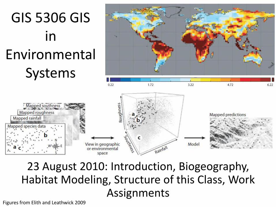
GIS 5306 GIS in Environmental Systems 23 August 2010: Introduction, Biogeography, Habitat Modeling, Structure of this Class, Work Assignments Figures from Elith and Leathwick 2009
Transcript of GIS 5306 GIS in Environmental Systems - CLAS Users
GIS 5306 GIS in
Environmental Systems
23 August 2010: Introduction, Biogeography, Habitat Modeling, Structure of this Class, Work
AssignmentsFigures from Elith and Leathwick 2009
GIS 5306 GIS Applications in Environmental Systems
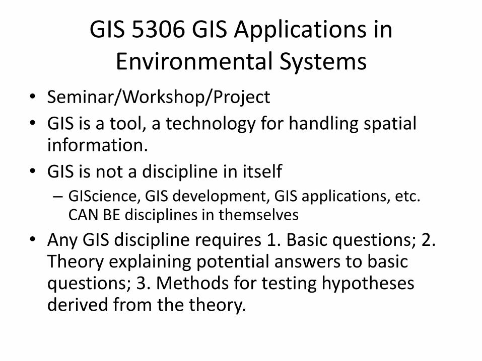
• Seminar/Workshop/Project
• GIS is a tool, a technology for handling spatial information.
• GIS is not a discipline in itself– GIScience, GIS development, GIS applications, etc.
CAN BE disciplines in themselves
• Any GIS discipline requires 1. Basic questions; 2. Theory explaining potential answers to basic questions; 3. Methods for testing hypotheses derived from the theory.
Course Objective
• For graduate students to learn how to use the tool of GIS and other technological methods, and the theory and methods of Species Distribution Modeling as an example of an advanced application of GIS and spatial thinking, well enough to teach it to other students and to apply it to their own research.
Dr. Michael W. [email protected]
http://www.clas.ufl.edu/users/mbinfordTurlington 3139
Office Hours Monday 4:00-5:00 PM, Tuesday 10:00-11:00 PM; and by appointment (e-mail me)
Fundamental Principles• All GIS uses require a project objective or a
research question, which are rooted in some practical issue or scientific theory, respectively. We’ll focus on a research question.
• The GIS user must understand the scientific theory AND the spatial theory relevant to the research question.
• Therefore, the GIS user must spend the effort to learn the theory, methods, and software in both the science and the technological aspects.
GIS 5306 GIS Applications in Environmental Systems
• From Syllabus: Note that for Fall 2010, we will study species habitat modeling, including forecasting effects of future climate change. The first part of the course will be an examination of different methods of habitat modeling, and the second part will be modeling specific habitats, of students' choosing, and possibly their potential changes due to climate change.
Figures from Elith and Leathwick 2009
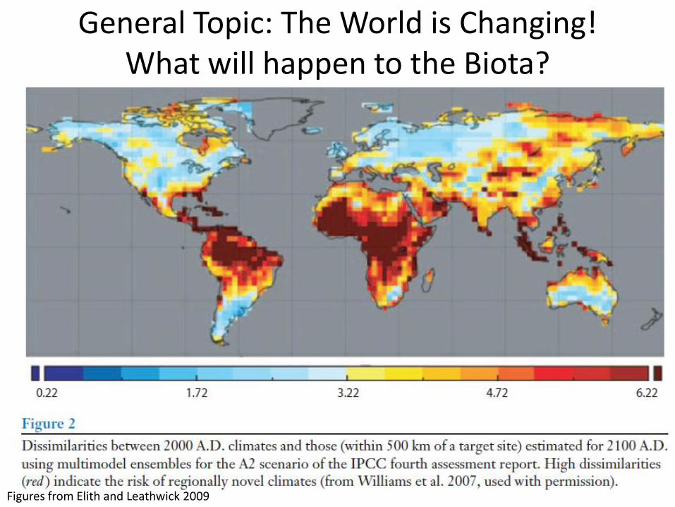
General Topic: The World is Changing! What will happen to the Biota?
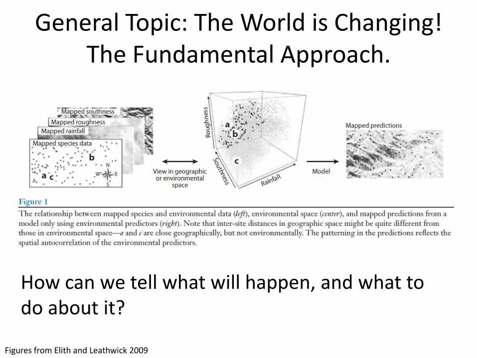
General Topic: The World is Changing! The Fundamental Approach.
How can we tell what will happen, and what to do about it?
Figures from Elith and Leathwick 2009
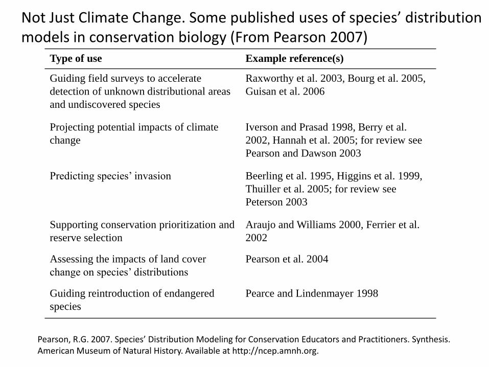
Not Just Climate Change. Some published uses of species’ distribution models in conservation biology (From Pearson 2007)
Type of use Example reference(s)
Guiding field surveys to accelerate
detection of unknown distributional areas
and undiscovered species
Raxworthy et al. 2003, Bourg et al. 2005,
Guisan et al. 2006
Projecting potential impacts of climate
change
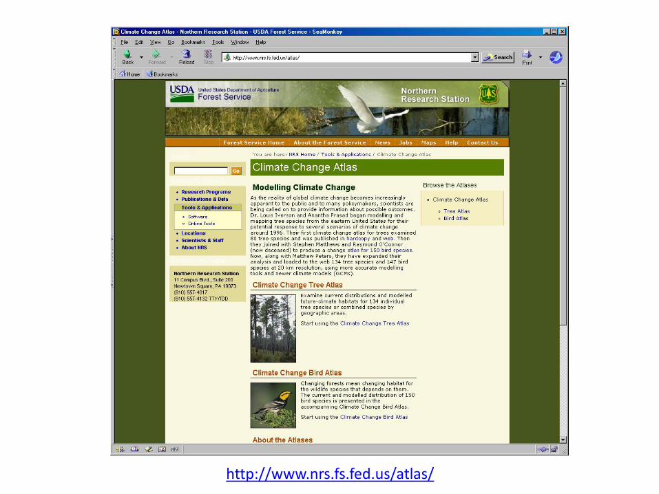
Iverson and Prasad 1998, Berry et al.
2002, Hannah et al. 2005; for review see
Pearson and Dawson 2003
Predicting species’ invasion Beerling et al. 1995, Higgins et al. 1999,
Thuiller et al. 2005; for review see
Peterson 2003
Supporting conservation prioritization and
reserve selection
Araujo and Williams 2000, Ferrier et al.
2002
Assessing the impacts of land cover
change on species’ distributions
Pearson et al. 2004
Guiding reintroduction of endangered
species
Pearce and Lindenmayer 1998
Pearson, R.G. 2007. Species’ Distribution Modeling for Conservation Educators and Practitioners. Synthesis. American Museum of Natural History. Available at http://ncep.amnh.org.
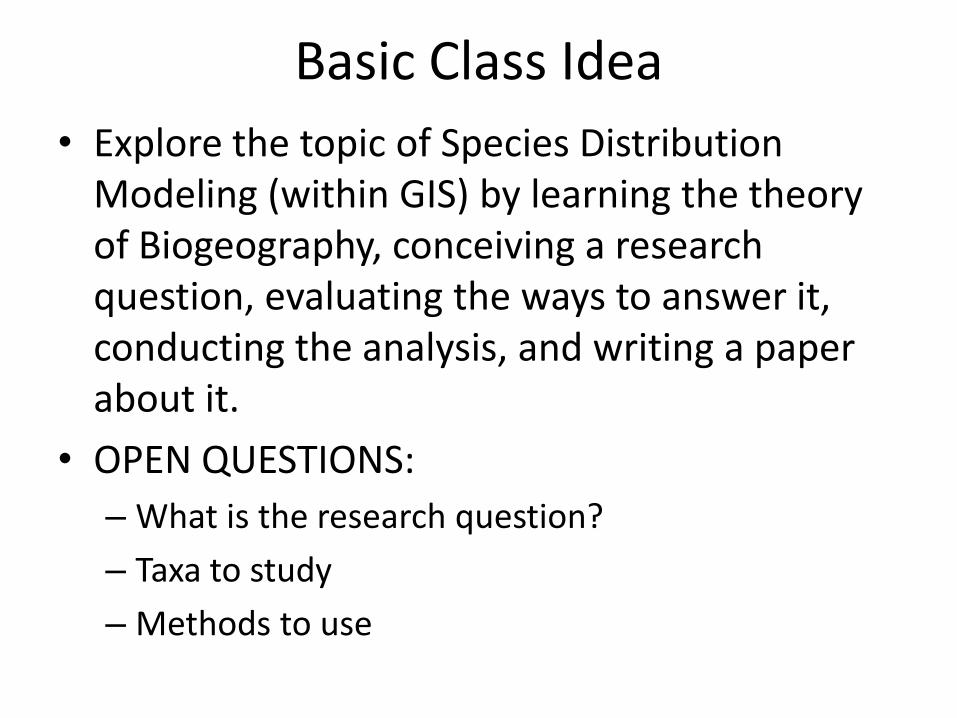
Basic Class Idea
• Explore the topic of Species Distribution Modeling (within GIS) by learning the theory of Biogeography, conceiving a research question, evaluating the ways to answer it, conducting the analysis, and writing a paper about it.
• OPEN QUESTIONS:
– What is the research question?
– Taxa to study
– Methods to use
Options – Multiple Student Teams or Class-as-a-whole Semester-long Project
• Option 1: Multiple Semester-long Projects by Students or Student Teams. Each of you, either individually or as a team no larger than three people, will conduct a semester-long project.
• Option 2: Whole-class project. The entire class will become a team that will conceive a research question, evaluate the ways to answer it, conduct the analysis, and write a paper about it.
Either Option
1. Either the class or each student (or student team) will develop a research question (or questions).
2. Each student will argue for a taxon or group of taxa to study, including the study area (Florida gets highest priority?).
3. When 1&2 are decided, Each student will then learn, evaluate, and teach one or more methods for studying the taxa to answer the research question to the class.
Basic Class Idea
• Each student (or team of 2 depending on the final size of the class) will become familiar with one or two of the methods for species distribution modeling, then present the theory of the method, the software for the method, and an example “laboratory exercise” to the class, including providing data for the exercise. This can be the tutorial produced by the developer of the software, or an exercise developed by the student(s).
Option 2
• When the methods have been examined, the class will decide the best methods and data required to answer the original research question.
• Then the whole class will conduct various aspects of the analysis (comparison of multiple methods?).
• Then we will write the paper, and submit it to an appropriate journal.
Work Assignments
• Instructor will conduct next week’s class:
– Theory of predictive vegetation mapping (subset of Species Distribution Modeling)
– Selection and description of one method for predictive vegetation mapping (logistic regression)
– Tutorial for working through a logistic regression example.
– Provision of data for working up several examples.
• Read the assigned papers linked on the syllabus.
Work Assignments• Over next 3 weeks, the instructor and two other experts
will go over their methods for SDM.• Students will, as pairs (?), do the same thing with other
theory, approaches, and workshops in the following sessions.
• Literature references categorized and online• At the beginning of next week’s class, each of you will
commit, with a partner (?), to lead one week’s class periods on one of the methods listed in the literature reference categories.– Prepare and present the theory description– Work through and understand the software and approach to the
problem.– Collect data appropriate for modeling, and developing a tutorial
for leading the rest of the students through the problem.
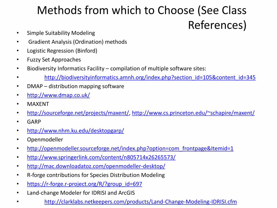
Methods from which to Choose (See Class References)
• Simple Suitability Modeling
• Gradient Analysis (Ordination) methods
• Logistic Regression (Binford)
• Fuzzy Set Approaches
• Biodiversity Informatics Facility – compilation of multiple software sites:
• http://biodiversityinformatics.amnh.org/index.php?section_id=105&content_id=345
• DMAP – distribution mapping software
• http://www.dmap.co.uk/
• MAXENT
• http://sourceforge.net/projects/maxent/, http://www.cs.princeton.edu/~schapire/maxent/
• GARP
• http://www.nhm.ku.edu/desktopgarp/
• Openmodeller
• http://openmodeller.sourceforge.net/index.php?option=com_frontpage&Itemid=1
• http://www.springerlink.com/content/n805714x26265573/
• http://mac.downloadatoz.com/openmodeller-desktop/
• R-forge contributions for Species Distribution Modeling
• https://r-forge.r-project.org/R/?group_id=697
• Land-change Modeler for IDRISI and ArcGIS
• http://clarklabs.netkeepers.com/products/Land-Change-Modeling-IDRISI.cfm
• Free GIS: DIVA-GIS: http://www.diva-gis.org/
One obvious research question, but not the only one.
• How will Florida become more susceptible to invasive plant species from the tropics under several of the scenarios presented by the IPCC report in 2007, or any newer ensembles of climate-change scenarios?
So, to help choose partners and for other reasons
• Who are you?
• What is your department? Your research interest?
• What is your background in GIS?
• What is your expectation for this class?
• What is something personal about you?

Who are you?
• Mike Binford
Fundamental References• Elith, Jane, and John R. Leathwick. 2009. Species
Distribution Models: Ecological Explanation and Prediction Across Space and Time. Annual Review of Ecology, Evolution, and Systematics 40, no. 1 (12): 677-697. doi: 10.1146/annurev.ecolsys.110308.120159. AND linked on syllabus web site
• Franklin, Janet. 2009. Mapping Species Distributions: Spatial Inference and Prediction (Ecology, Biodiversity and Conservation). Cambridge University Press. THE UF LIBRARY DOES NOT HAVE THIS BOOK. I’VE ORDERED IT. WHEN IT COMES IN I’LL PUT A COPY ON RESERVE.
• Lomolino, M.V. B.R. Riddle, J.H. Brown. Biogeography. Sinauer. 3rd ed. 845 pp. Not on reserve.

Other Logistics
• Dr. Michael W. Binford
• www.clas.ufl.edu/users/mbinford
• Turlington 3139
• Office Hours 4:00-5:00 Mondays; 10:00-11:00 Tuesdays, or by Appointment
• Accounts generated from registrar’s data. Can you log on now? (Use Gatorlink ID and password.)
Back To: The Question(s) In This Class
• How are organisms distributed on the surface of the Earth, and why?
• As Earth’s environment changes (climate, land use, geomorphologic, geologic, biologic), how will the distribution of organisms change?
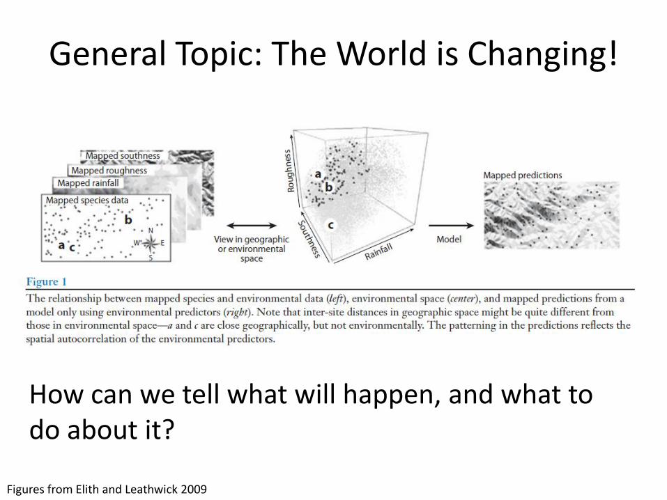
General Topic: The World is Changing!
How can we tell what will happen, and what to do about it?
Figures from Elith and Leathwick 2009
Structure of Course
• Basic questions have been asked.
• Each class meeting (After this one) for the first part of the class will consist of:– Description of theory explaining potential answers
to basic questions.
– Description of methods for testing hypotheses derived from the theory.
– Workshop in which we work through examples
• Second part of the class will be working on the project (or projects).
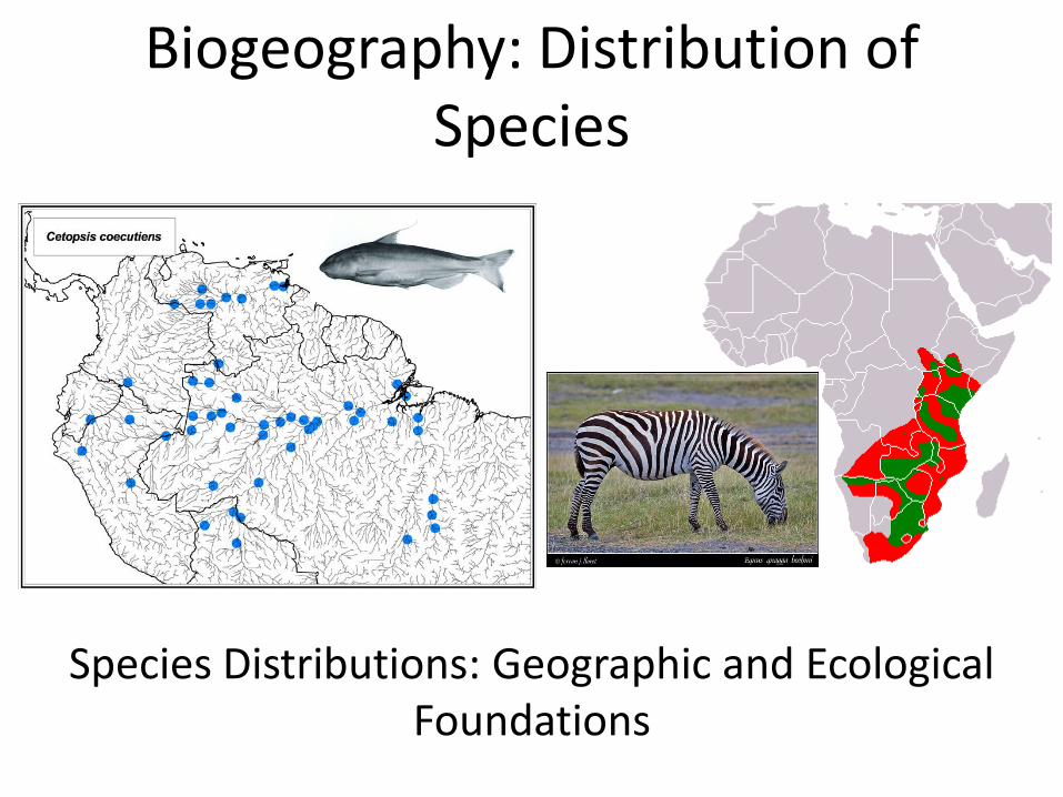
Biogeography: Distribution of Species
Species Distributions: Geographic and Ecological Foundations
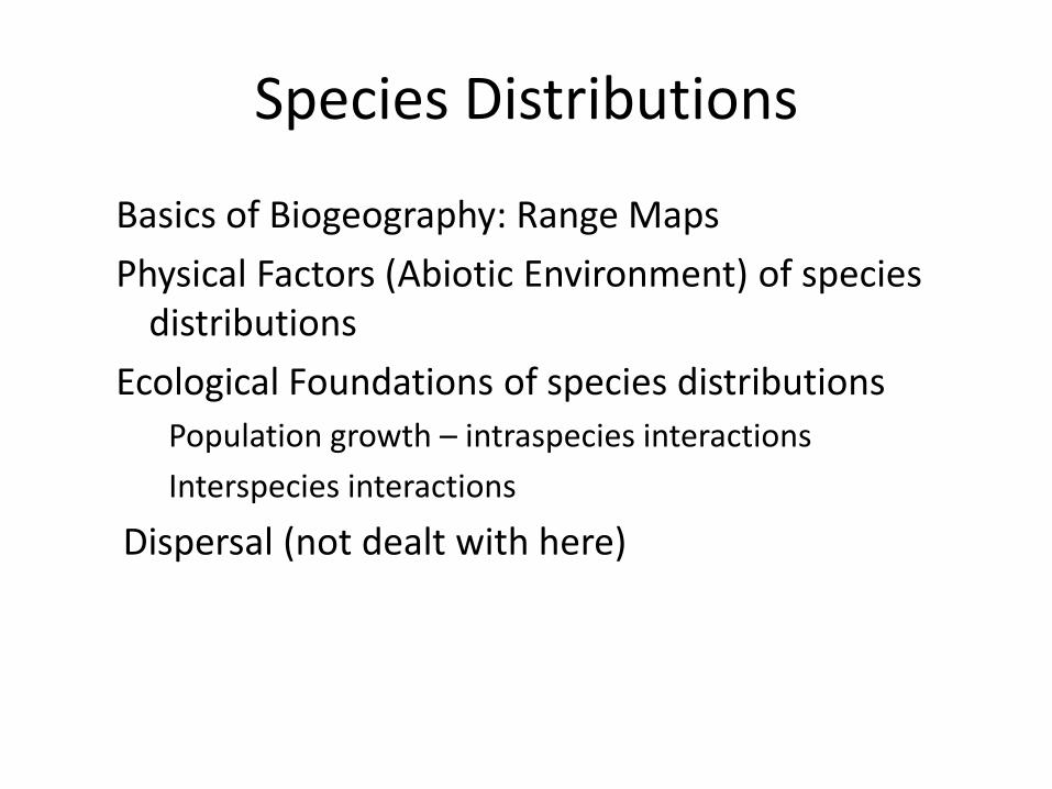
Species Distributions
Basics of Biogeography: Range Maps
Physical Factors (Abiotic Environment) of species distributions
Ecological Foundations of species distributions
Population growth – intraspecies interactions
Interspecies interactions
Dispersal (not dealt with here)
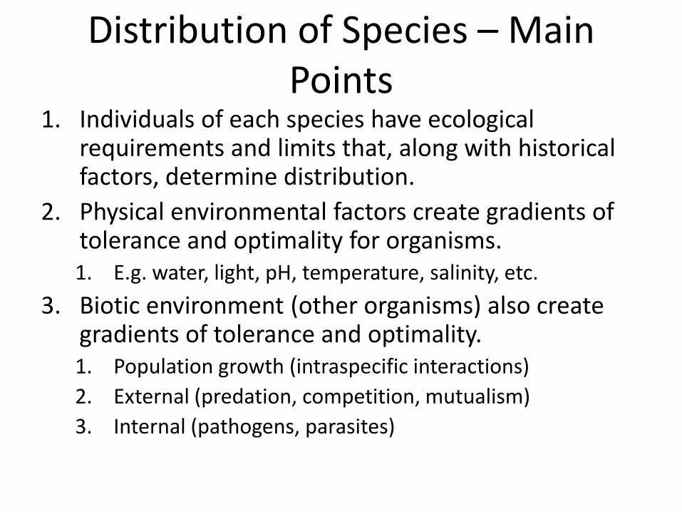
Distribution of Species – Main Points
1. Individuals of each species have ecological requirements and limits that, along with historical factors, determine distribution.
2. Physical environmental factors create gradients of tolerance and optimality for organisms.1. E.g. water, light, pH, temperature, salinity, etc.
3. Biotic environment (other organisms) also create gradients of tolerance and optimality.1. Population growth (intraspecific interactions)
2. External (predation, competition, mutualism)
3. Internal (pathogens, parasites)
New Topic: Distribution of Species – Secondary Points
1. Interactions of physical and biotic factors always occur.
2. Very difficult to demonstrate mechanisms of distribution limitation, but straightforward to show correlations among physical and biotic factors and distributions.
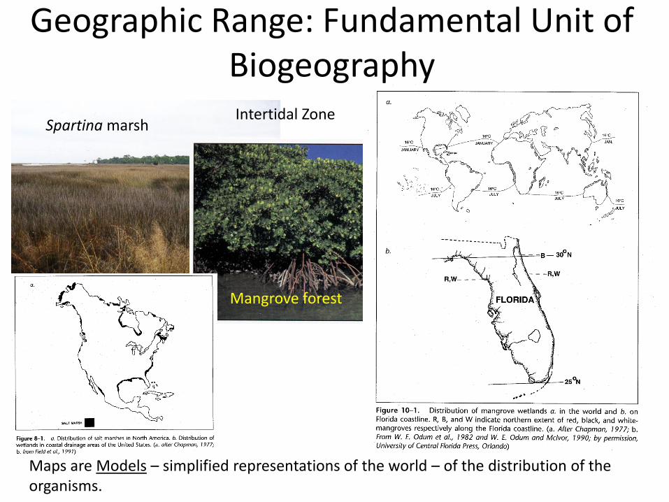
Geographic Range: Fundamental Unit of Biogeography
Spartina marshIntertidal Zone
Mangrove forest
Maps are Models – simplified representations of the world – of the distribution of the organisms.
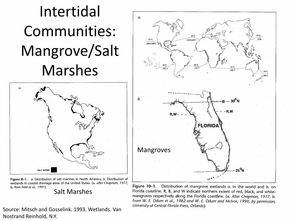
Intertidal Communities: Mangrove/Salt
Marshes
Source: Mitsch and Gosselink. 1993. Wetlands. Van Nostrand Reinhold, N.Y.
Salt Marshes
Mangroves
Range Maps
• Dot
• Outline
• Contour
• Combinations
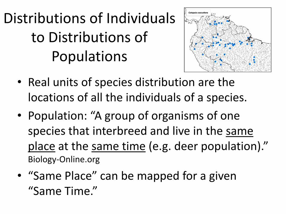
Distributions of Individuals to Distributions of
Populations
• Real units of species distribution are the locations of all the individuals of a species.
• Population: “A group of organisms of one species that interbreed and live in the same place at the same time (e.g. deer population).” Biology-Online.org
• “Same Place” can be mapped for a given “Same Time.”
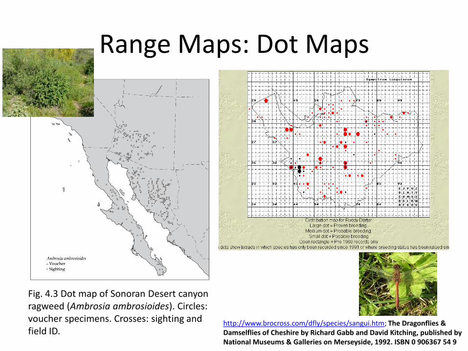
Range Maps: Dot Maps
Fig. 4.3 Dot map of Sonoran Desert canyon ragweed (Ambrosia ambrosioides). Circles: voucher specimens. Crosses: sighting and field ID.
http://www.brocross.com/dfly/species/sangui.htm; The Dragonflies & Damselflies of Cheshire by Richard Gabb and David Kitching, published by National Museums & Galleries on Merseyside, 1992. ISBN 0 906367 54 9
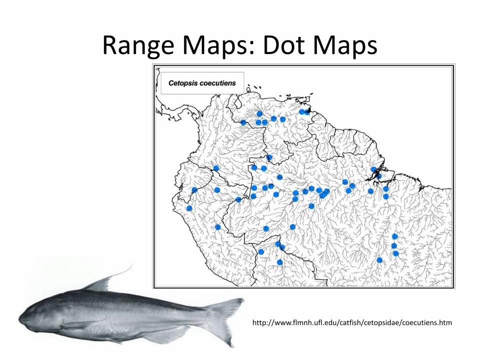
Range Maps: Dot Maps
http://www.flmnh.ufl.edu/catfish/cetopsidae/coecutiens.htm
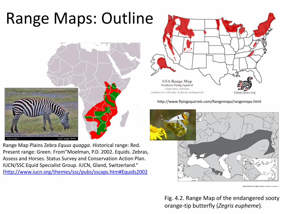
Range Maps: Outline
Range Map Plains Zebra Equus quagga. Historical range: Red. Present range: Green. From"Moelman, P.D. 2002. Equids. Zebras, Assess and Horses. Status Survey and Conservation Action Plan. IUCN/SSC Equid Specialist Group. IUCN, Gland, Switzerland.“ (http://www.iucn.org/themes/ssc/pubs/sscaps.htm#Equids2002
http://www.flyingsquirrels.com/Rangemaps/rangemaps.html
Fig. 4.2. Range Map of the endangered sooty orange-tip butterfly (Zegris eupheme).
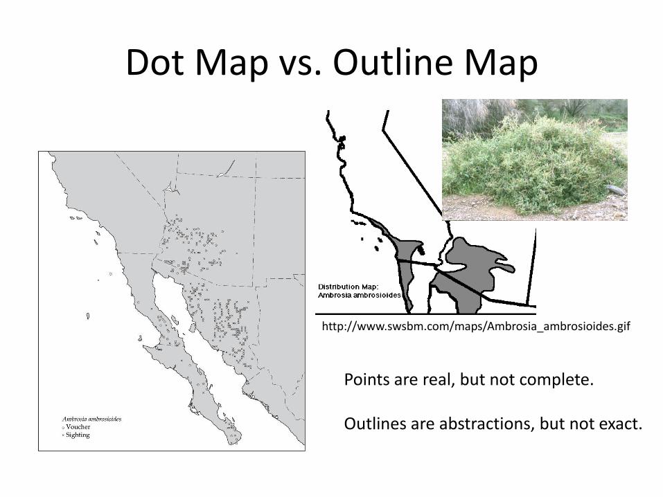
Dot Map vs. Outline Map
http://www.swsbm.com/maps/Ambrosia_ambrosioides.gif
Points are real, but not complete.
Outlines are abstractions, but not exact.
Range Maps: Contour or Surface
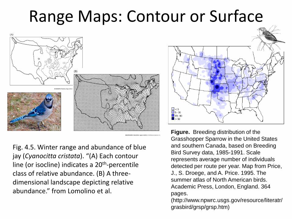
Fig. 4.5. Winter range and abundance of blue jay (Cyanocitta cristata). “(A) Each contour line (or isocline) indicates a 20th-percentile class of relative abundance. (B) A three-dimensional landscape depicting relative abundance.” from Lomolino et al.
Figure. Breeding distribution of the
Grasshopper Sparrow in the United States
and southern Canada, based on Breeding
Bird Survey data, 1985-1991. Scale
represents average number of individuals
detected per route per year. Map from Price,
J., S. Droege, and A. Price. 1995. The
summer atlas of North American birds.
Academic Press, London, England. 364
pages.
(http://www.npwrc.usgs.gov/resource/literatr/
grasbird/grsp/grsp.htm)
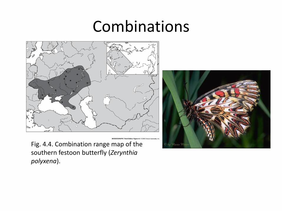
Combinations
Fig. 4.4. Combination range map of the southern festoon butterfly (Zerynthiapolyxena).
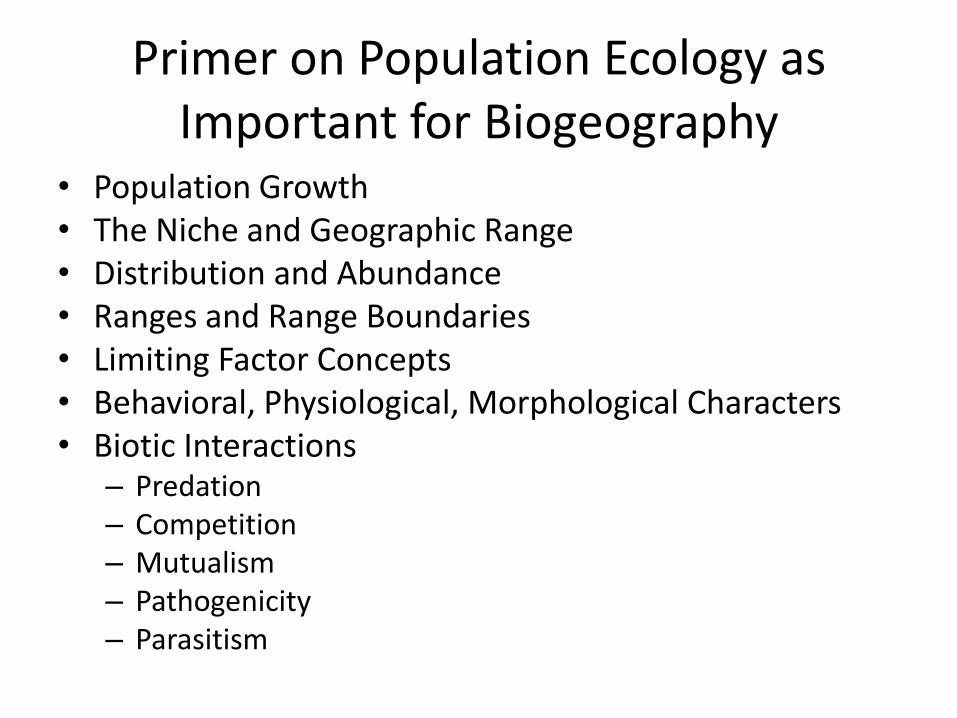
Primer on Population Ecology as Important for Biogeography
• Population Growth• The Niche and Geographic Range• Distribution and Abundance• Ranges and Range Boundaries• Limiting Factor Concepts• Behavioral, Physiological, Morphological Characters• Biotic Interactions
– Predation– Competition– Mutualism– Pathogenicity– Parasitism
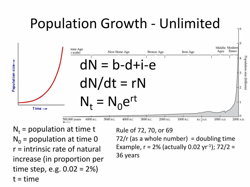
Population Growth - Unlimited
dN = b-d+i-edN/dt = rNNt = N0ert
Nt = population at time tN0 = population at time 0r = intrinsic rate of natural increase (in proportion per time step, e.g. 0.02 = 2%)t = time
Rule of 72, 70, or 6972/r (as a whole number) = doubling timeExample, r = 2% (actually 0.02 yr-1); 72/2 = 36 years
What Influences r?
• Resources
• Physiological process rates (temperature, environmental chemistry)
• # of offspring in each generation
• Survivorship of offspring to reproduction (generation)
• Health of organisms
• Many other factors

Logistic Growth – Density-dependent Limit
K = “Carrying Capacity” in units of individuals
Nt = N0er((K-N)/K)t
http://www.cals.ncsu.edu/course/fw353/Yield.htm
dN/dt = f(N) = rN((K-N)/K)
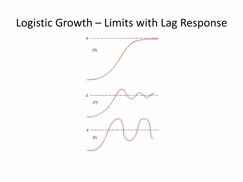
Logistic Growth – Limits with Lag Response
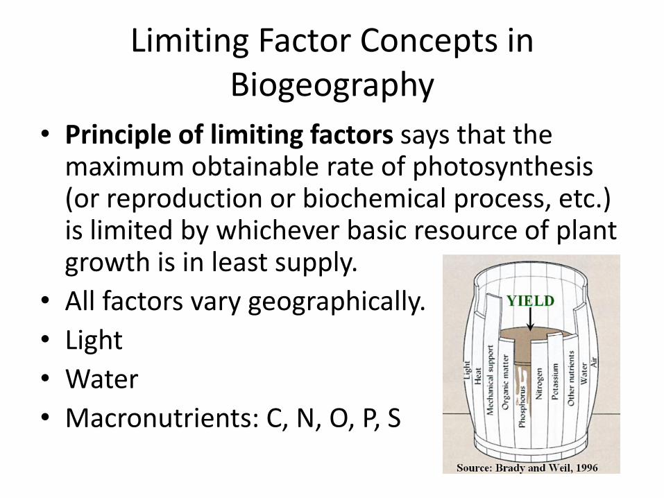
Limiting Factor Concepts in Biogeography
• Principle of limiting factors says that the maximum obtainable rate of photosynthesis (or reproduction or biochemical process, etc.) is limited by whichever basic resource of plant growth is in least supply.
• All factors vary geographically.
• Light
• Water
• Macronutrients: C, N, O, P, S
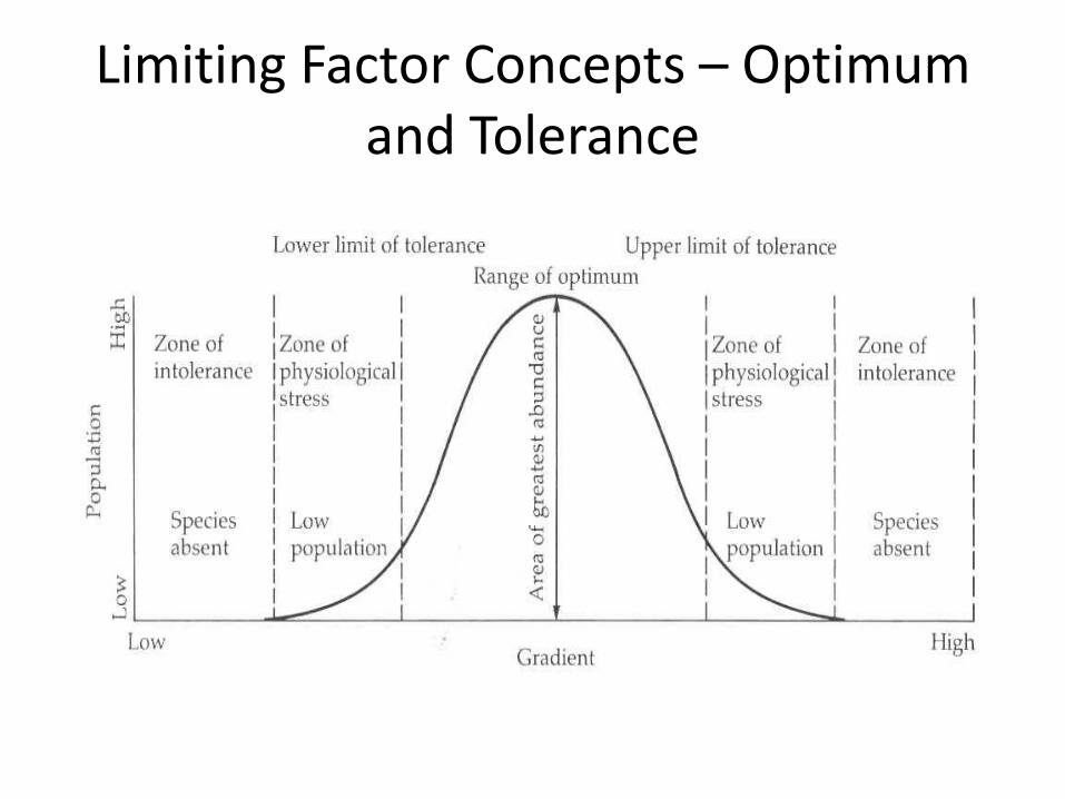
Limiting Factor Concepts – Optimum and Tolerance
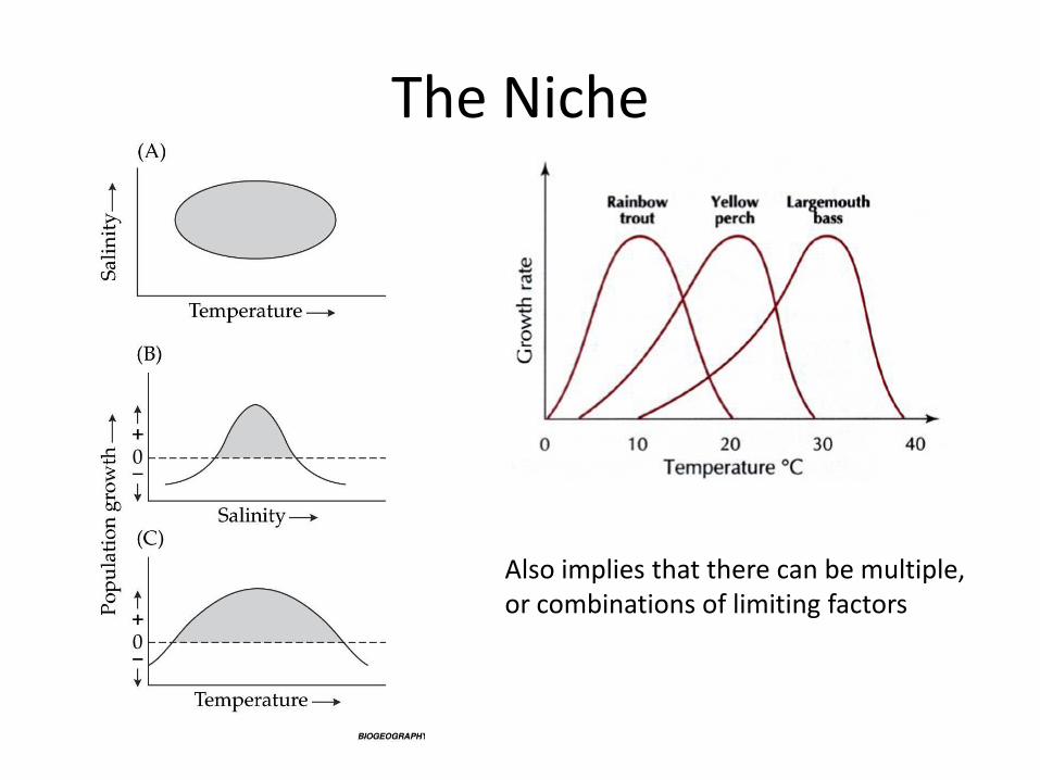
The Niche
Also implies that there can be multiple, or combinations of limiting factors

The Niche and Geographic Range
Predator Density
Salinity
Rothschild, B.J. et al. 1994. Decline of the Chesapeake Bay Oyster population: a century of habitat destruction and overfishing. Marine Ecology Progress Series 111:29-39.
n-Dimensional Hypervolume
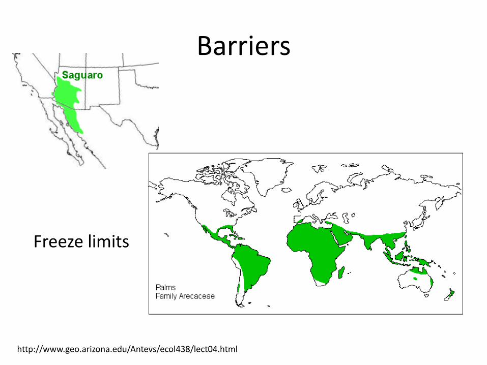
Barriers
Freeze limits
http://www.geo.arizona.edu/Antevs/ecol438/lect04.html
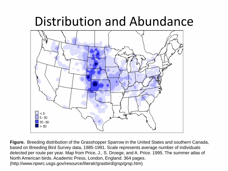
Distribution and Abundance
Figure. Breeding distribution of the Grasshopper Sparrow in the United States and southern Canada,
based on Breeding Bird Survey data, 1985-1991. Scale represents average number of individuals
detected per route per year. Map from Price, J., S. Droege, and A. Price. 1995. The summer atlas of
North American birds. Academic Press, London, England. 364 pages.
(http://www.npwrc.usgs.gov/resource/literatr/grasbird/grsp/grsp.htm)
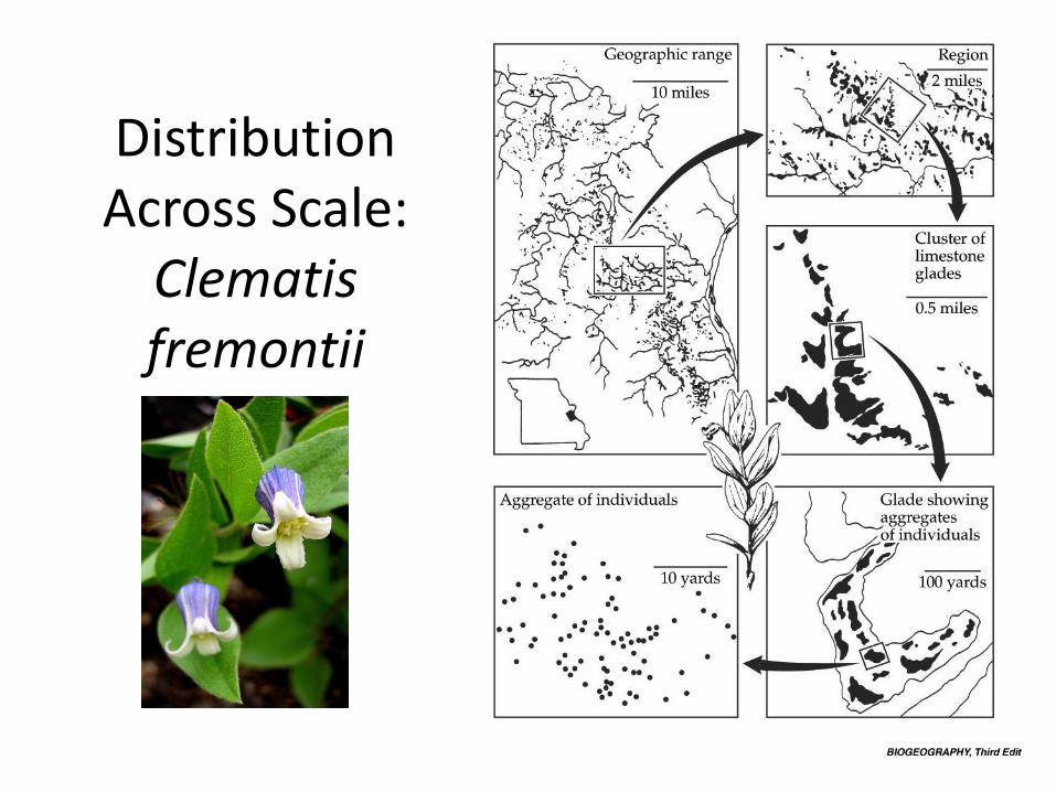
Distribution Across Scale:
Clematis fremontii
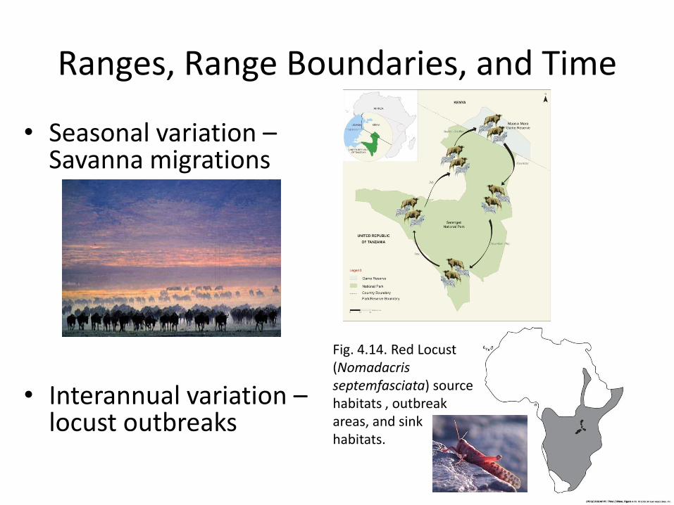
Ranges, Range Boundaries, and Time
• Seasonal variation –Savanna migrations
• Interannual variation –locust outbreaks
Fig. 4.14. Red Locust (Nomadacrisseptemfasciata) source habitats , outbreak areas, and sink habitats.
Biotic Interactions
• Predation
• Competition
• Mutualism
• Pathogenicity
• Parasitism
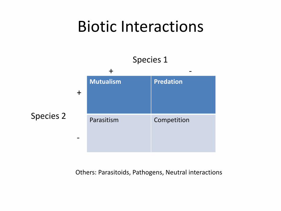
Biotic Interactions
Mutualism Predation
Parasitism Competition
Species 1+ -
Species 2
+
-
Others: Parasitoids, Pathogens, Neutral interactions
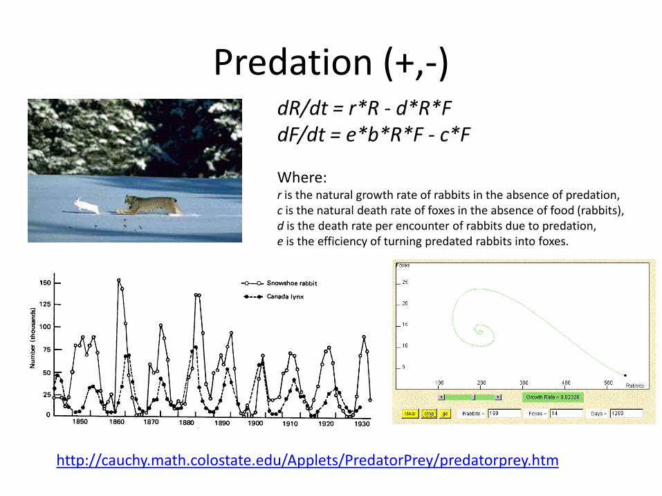
Predation (+,-)
http://cauchy.math.colostate.edu/Applets/PredatorPrey/predatorprey.htm
dR/dt = r*R - d*R*FdF/dt = e*b*R*F - c*F
Where: r is the natural growth rate of rabbits in the absence of predation, c is the natural death rate of foxes in the absence of food (rabbits), d is the death rate per encounter of rabbits due to predation, e is the efficiency of turning predated rabbits into foxes.
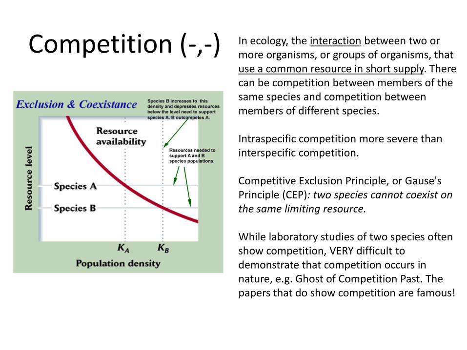
Competition (-,-) In ecology, the interaction between two or more organisms, or groups of organisms, that use a common resource in short supply. There can be competition between members of the same species and competition between members of different species.
Intraspecific competition more severe than interspecific competition.
Competitive Exclusion Principle, or Gause'sPrinciple (CEP): two species cannot coexist on the same limiting resource.
While laboratory studies of two species often show competition, VERY difficult to demonstrate that competition occurs in nature, e.g. Ghost of Competition Past. The papers that do show competition are famous!
Others
• Mutualism– Obligate
– Facultative
• Parasitism– Don’t kill the host!
– Parasitoids – kill the host!
• Pathogenicity– Morbidity
– Mortality
Some Example Species Distribution Models
• Vegetation – plants
• Animals
– Habitat suitability index models
– wildlife-habitat relationship models
• Disease pathogens • Habitat
• Organisms
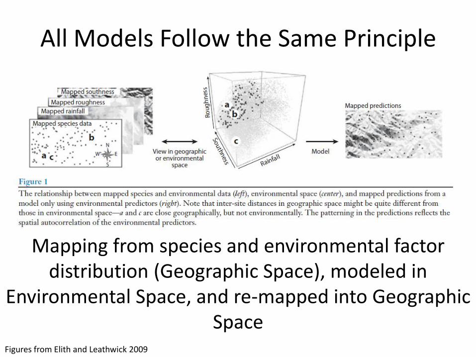
All Models Follow the Same Principle
Mapping from species and environmental factor distribution (Geographic Space), modeled in
Environmental Space, and re-mapped into Geographic Space
Figures from Elith and Leathwick 2009
From Austin 2007• The components are: (1) an ecological model
concerning the ecological theory used or assumed,
• (2) a data model concerning the type of data used and method of data collection and
• (3) a statistical model concerning the statistical methods and theory applied (Austin, 2002a).
From Austin 2007• Non-statistical methods of prediction such as
neural nets (Fitzgerald and Lees, 1992), GARP (Stockwell and Noble, 1992) and climatic envelopes (Pearson and Dawson, 2003) are not considered though see Elith et al. (2006).
• Elith, J., et al., 2006. Novel methods improve prediction of species distributions from occurrence data. Ecography 29, 129–151.
From Austin 2007, about statistical methods, esp. GLM, GAM
• General Linear Models (regression, logistic regression), General Additive Models
• What ecological theory is assumed or tested?
• Are there any limitations imposed by the nature of the data used?
• Are the statistical procedures and methods used compatible
• with ecological theory?
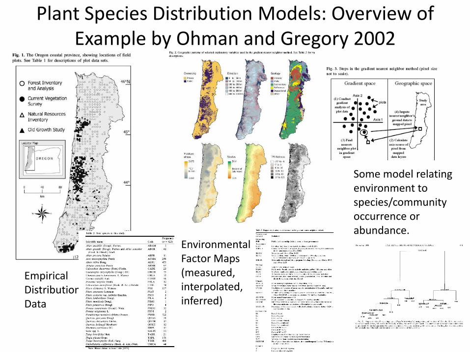
Plant Species Distribution Models: Overview of Example by Ohman and Gregory 2002
Empirical Distribution Data
Environmental Factor Maps (measured, interpolated, inferred)
Some model relating environment to species/community occurrence or abundance.

Plant Species Distribution Models: Results
Dominant Environmental Gradients Mapped
Predicted Vegetation Classes
Model Analysis Results (Gradient Analysis by Correspondence Analysis)
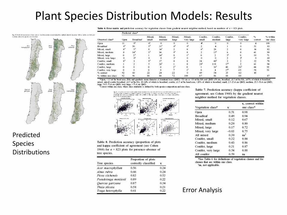
Plant Species Distribution Models: Results
Predicted Species Distributions
Error Analysis
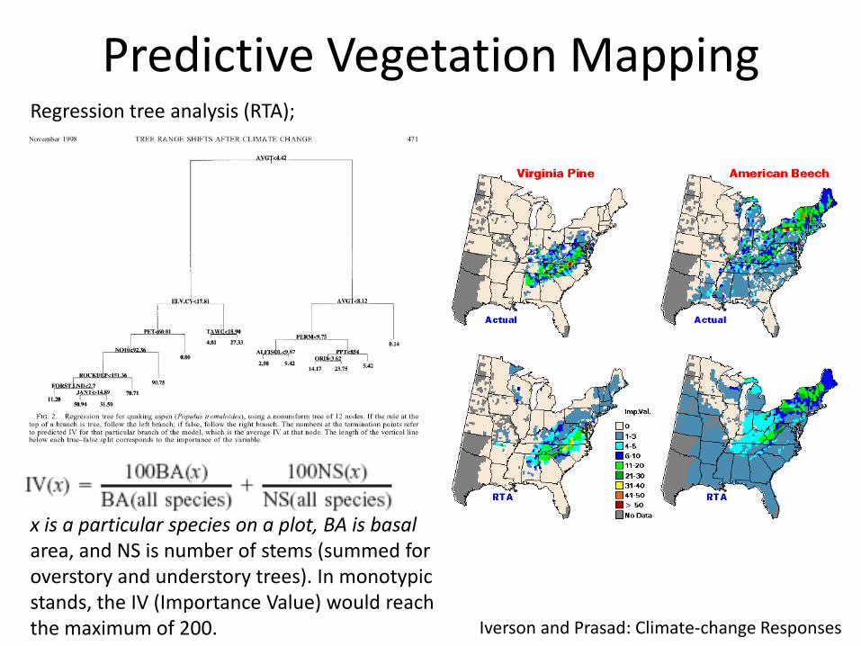
Predictive Vegetation Mapping
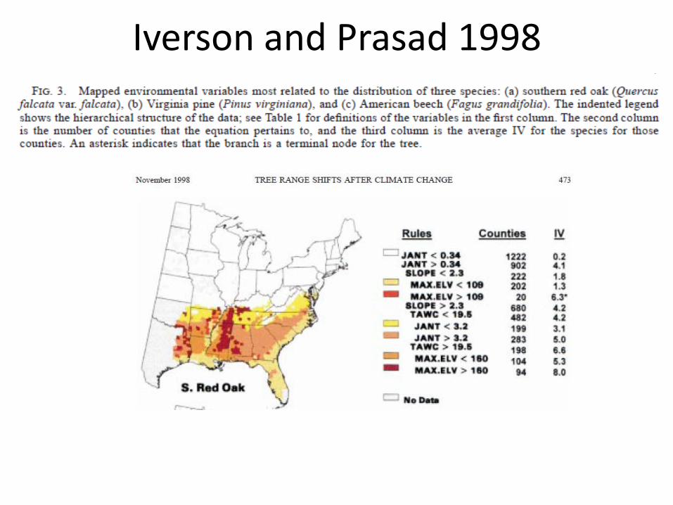
Iverson and Prasad: Climate-change Responses
Regression tree analysis (RTA);
x is a particular species on a plot, BA is basal area, and NS is number of stems (summed for overstory and understory trees). In monotypic stands, the IV (Importance Value) would reach the maximum of 200.
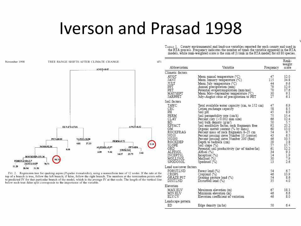
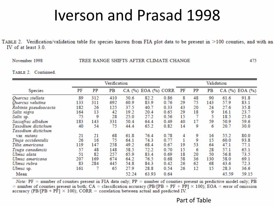
Iverson and Prasad 1998
Iverson and Prasad 1998
Iverson and Prasad 1998
Part of Table
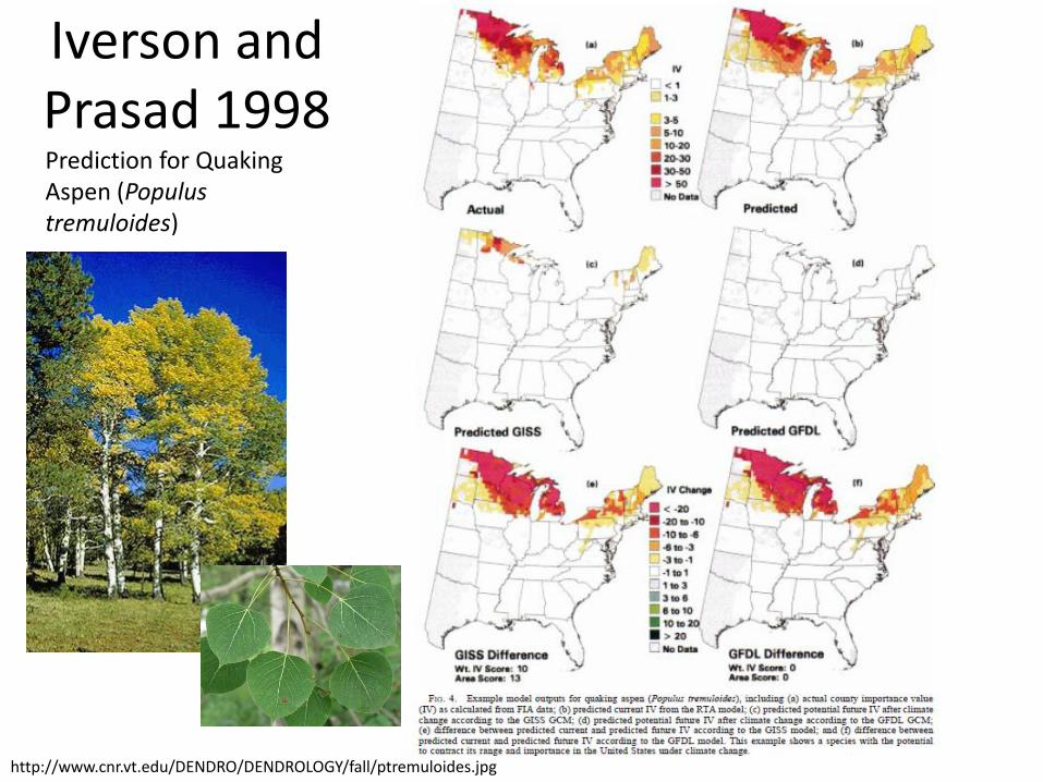
Iverson and Prasad 1998Prediction for Quaking Aspen (Populustremuloides)
http://www.cnr.vt.edu/DENDRO/DENDROLOGY/fall/ptremuloides.jpg
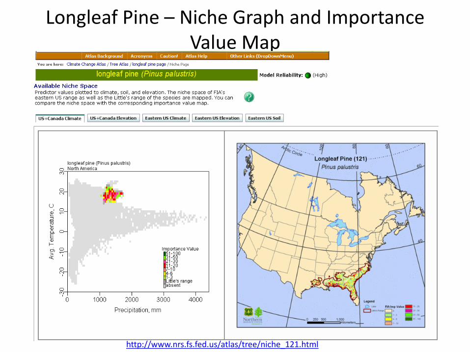
Longleaf Pine – Niche Graph and Importance Value Map
http://www.nrs.fs.fed.us/atlas/tree/niche_121.html
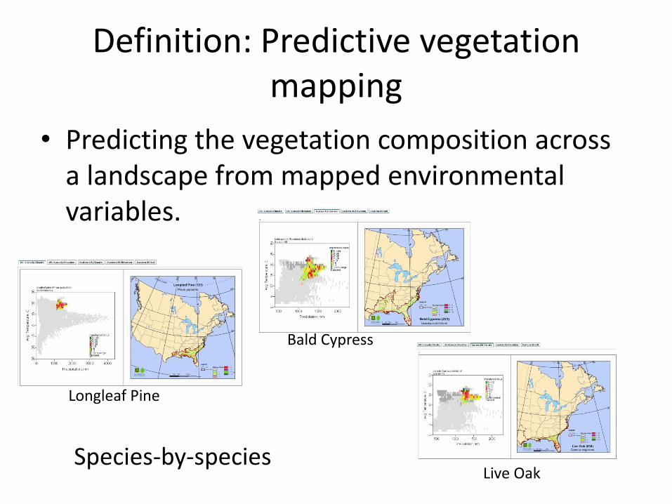
Definition: Predictive vegetation mapping
• Predicting the vegetation composition across a landscape from mapped environmental variables.
Species-by-species
Longleaf Pine
Bald Cypress
Live Oak
Predictive vegetation mapping: Franklin 1995
• Fundamental paper reviewing practice to 1994
• Principles of Predictive Species Distribution Modeling (PSDM)
– Predictive Vegetation Mapping
– Habitat Modeling
• Dependence of predictive vegetation mapping on ecological niche theory and gradient analysis
• Cited by 363 more recent papers
Franklin 1995
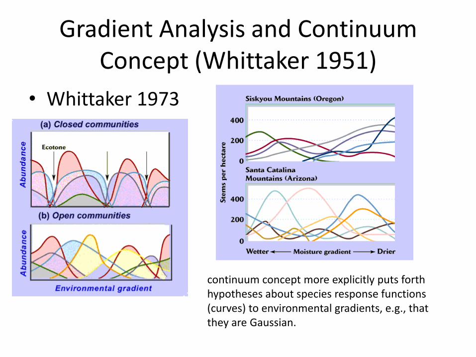
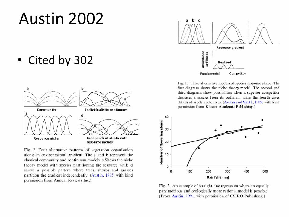
Gradient Analysis and Continuum Concept (Whittaker 1951)
• Whittaker 1973
continuum concept more explicitly puts forth hypotheses about species response functions(curves) to environmental gradients, e.g., that they are Gaussian.

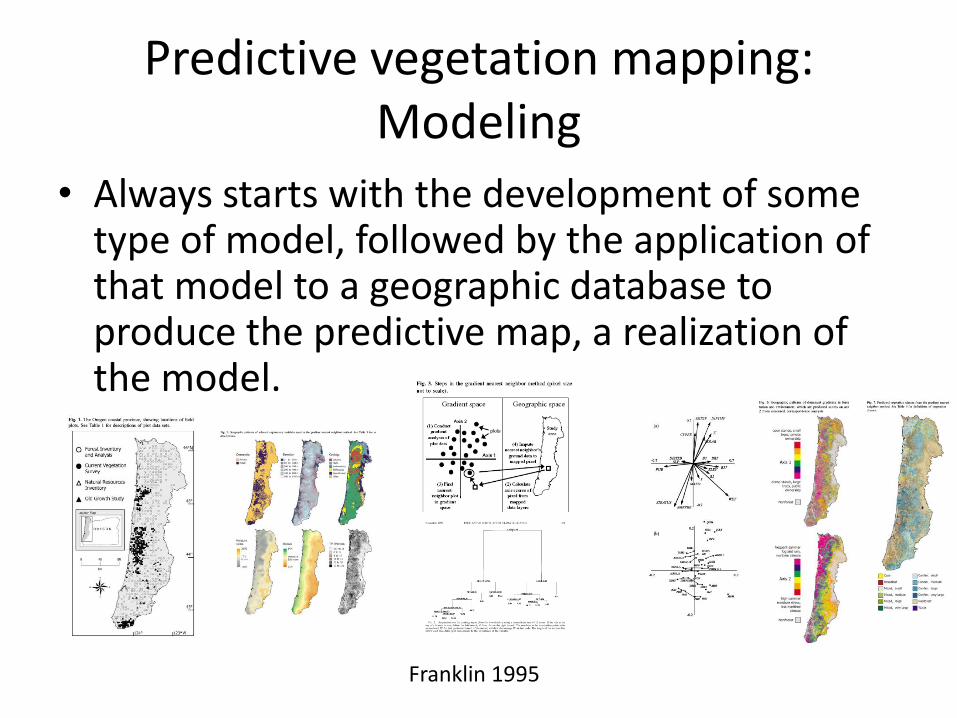
Predictive vegetation mapping: Modeling
• Always starts with the development of some type of model, followed by the application of that model to a geographic database to produce the predictive map, a realization of the model.
Franklin 1995

Foundations and Premises
• Predictive vegetation mapping is founded in ecological niche theory and vegetation gradient analysis.
• Premise: vegetation distribution can be predicted from the spatial distribution of environmental variables that correlate with or control plant distributions.
Franklin 1995

Pragmatism
• Further, maps of the environmental variables or their surrogates must be available, or easier to map than the vegetation itself, in order for predictive vegetation mapping to be a practical or informative exercise.
Franklin 1995

Model Foundations
• In order to extrapolate over space (predictive vegetation mapping) or time (vegetation change modeling), direct gradients or their surrogates must be mapped (temperature, potential solar radiation, precipitation, soil-moisture availability, geology or soil chemistry).

Spatial Focus
• Focus on the prediction of plant species distributions or vegetation patterns at the 'regional' scale, e.g., where the mapped extent of the predictions are generally at or within the biogeographic range of the dominant plant species.
Franklin 1995
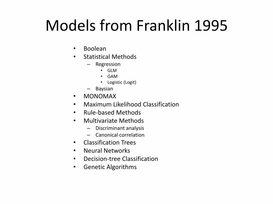
Models from Franklin 1995• Boolean• Statistical Methods
– Regression• GLM• GAM• Logistic (Logit)
– Baysian
• MONOMAX• Maximum Likelihood Classification• Rule-based Methods• Multivariate Methods
– Discriminant analysis– Canonical correlation
• Classification Trees• Neural Networks• Decision-tree Classification• Genetic Algorithms
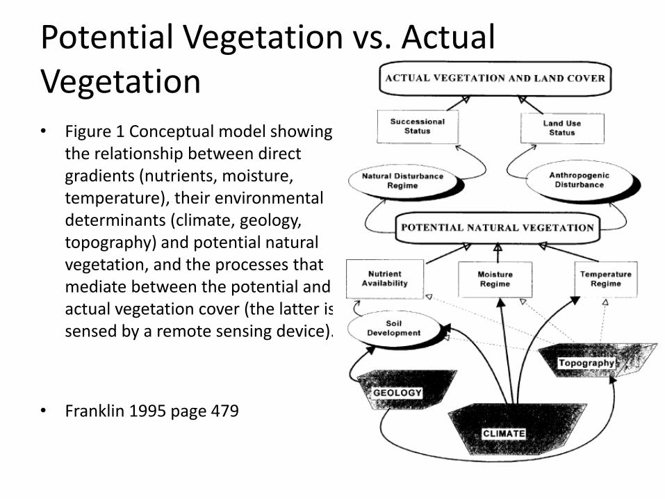
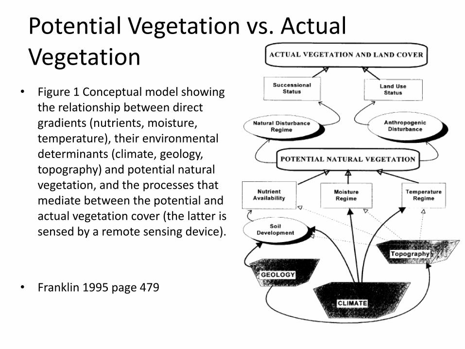
Potential Vegetation vs. Actual Vegetation• Figure 1 Conceptual model showing
the relationship between direct gradients (nutrients, moisture, temperature), their environmental determinants (climate, geology, topography) and potential natural vegetation, and the processes that mediate between the potential and actual vegetation cover (the latter is sensed by a remote sensing device).
• Franklin 1995 page 479

Austin 2002
• Cited by 302
New Lecture: This time
• Predictive vegetation mapping -fundamentals
• Species distribution models• Wildlife-Habitat Relationship
Models• Habitat suitability indices• Note: new readings.
– GAP Handbook– Classical example of Gradient
Analysis
Principal
• If species’ ranges are the basic units of biogeography, and
• Species range maps are the basic measurement, but
• Species range maps are notoriously innaccurateor imprecise (dots vs. areas vs. contour vs. combinations) and do not consider environmental spatial heterogeneity, then
• Some sort of modeling might give us better estimates of species’ distributions.

Predictive vegetation mapping: Franklin 1995
• Fundamental paper reviewing practice to 1994
• Principles of Predictive Species Distribution Modeling (PSDM)
– Predictive Vegetation Mapping
– Habitat Modeling
• Dependence of predictive vegetation mapping on ecological niche theory and gradient analysis
• Cited by 366 more recent papers
Franklin 1995

Predictive vegetation mapping: Modeling
• Always starts with the development of some type of model, followed by the application of that model to a geographic database to produce the predictive map, a realization of the model.
Franklin 1995
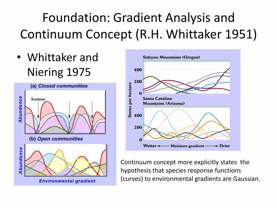
Foundation: Gradient Analysis and Continuum Concept (R.H. Whittaker 1951)
• Whittaker and Niering 1975
Continuum concept more explicitly states the hypothesis that species response functions(curves) to environmental gradients are Gaussian.
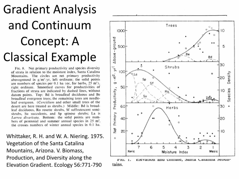
Gradient Analysis and Continuum
Concept: A Classical Example
Whittaker, R. H. and W. A. Niering. 1975. Vegetation of the Santa Catalina Mountains, Arizona. V. Biomass, Production, and Diversity along the Elevation Gradient. Ecology 56:771-790
Predictive vegetation mapping: Modeling
• Always starts with the development of some type of model, followed by the application of that model to a geographic database to produce the predictive map, a realization of the model.
Franklin 1995
Foundations and Premises
• Predictive vegetation mapping is founded in ecological niche theory and vegetation gradient analysis.
• Premise: vegetation distribution can be predicted from the spatial distribution of environmental variables that correlate with or control plant distributions.
Franklin 1995
Pragmatism
• Further, maps of the environmental variables or their surrogates must be available, or easier to map than the vegetation itself, in order for predictive vegetation mapping to be a practical or informative exercise.
Franklin 1995
Model Foundations
• In order to extrapolate over space (predictive vegetation mapping) or time (vegetation change modelling), direct gradients or their surrogates must be mapped (temperature, potential solar radiation, precipitation, soil-moisture availability, geology or soil chemistry).
Spatial Focus
• Focus on the prediction of plant species distributions or vegetation patterns at the 'regional' scale, e.g., where the mapped extent of the predictions are generally at or within the biogeographic range of the dominant plant species.
Franklin 1995
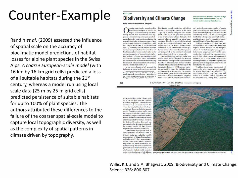
Counter-Example
Randin et al. (2009) assessed the influence of spatial scale on the accuracy of bioclimatic model predictions of habitat losses for alpine plant species in the Swiss Alps. A coarse European-scale model (with 16 km by 16 km grid cells) predicted a loss of all suitable habitats during the 21st
century, whereas a model run using local scale data (25 m by 25 m grid cells) predicted persistence of suitable habitats for up to 100% of plant species. The authors attributed these differences to the failure of the coarser spatial-scale model to capture local topographic diversity, as well as the complexity of spatial patterns in climate driven by topography.
Willis, K.J. and S.A. Bhagwat. 2009. Biodiversity and Climate Change. Science 326: 806-807

Models from Franklin 1995• Boolean (Set Theory)• Statistical Methods
– Regression• GLM• GAM• Logistic (Logit)
– Bayseian
• MONOMAX• Maximum Likelihood
Classification• Rule-based Methods• Multivariate Methods
– Discriminant analysis– Canonical correlation
• Classification Trees• Neural Networks• Decision-tree Classification• Genetic Algorithms
Potential Vegetation vs. Actual Vegetation
• Figure 1 Conceptual model showing the relationship between direct gradients (nutrients, moisture, temperature), their environmental determinants (climate, geology, topography) and potential natural vegetation, and the processes that mediate between the potential and actual vegetation cover (the latter is sensed by a remote sensing device).
• Franklin 1995 page 479
Austin 2002
• Cited by 302
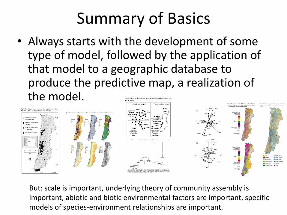
Summary of Basics• Always starts with the development of some
type of model, followed by the application of that model to a geographic database to produce the predictive map, a realization of the model.
But: scale is important, underlying theory of community assembly is important, abiotic and biotic environmental factors are important, specific models of species-environment relationships are important.
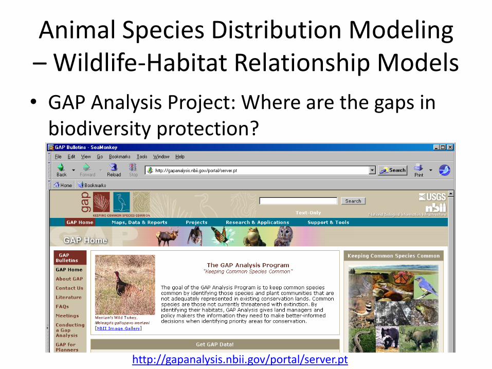
Animal Species Distribution Modeling – Wildlife-Habitat Relationship Models
• GAP Analysis Project: Where are the gaps in biodiversity protection?
http://gapanalysis.nbii.gov/portal/server.pt

GAP Procedures
Note WHRM is an associational
database: what animals would be
expected to be found in vegetation alliance (habitat).
From Complete GAP Handbook available from ftp://ftp.gap.uidaho.edu/products/handbookpdf/CompleteHandbook.pdf
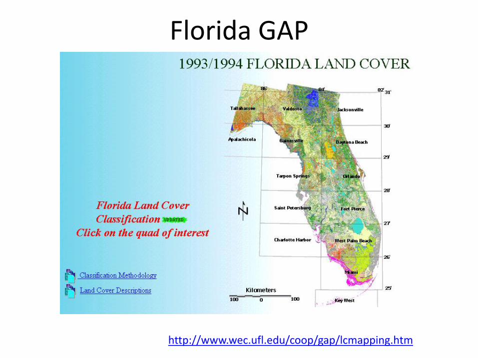
Florida GAP
http://www.wec.ufl.edu/coop/gap/lcmapping.htm
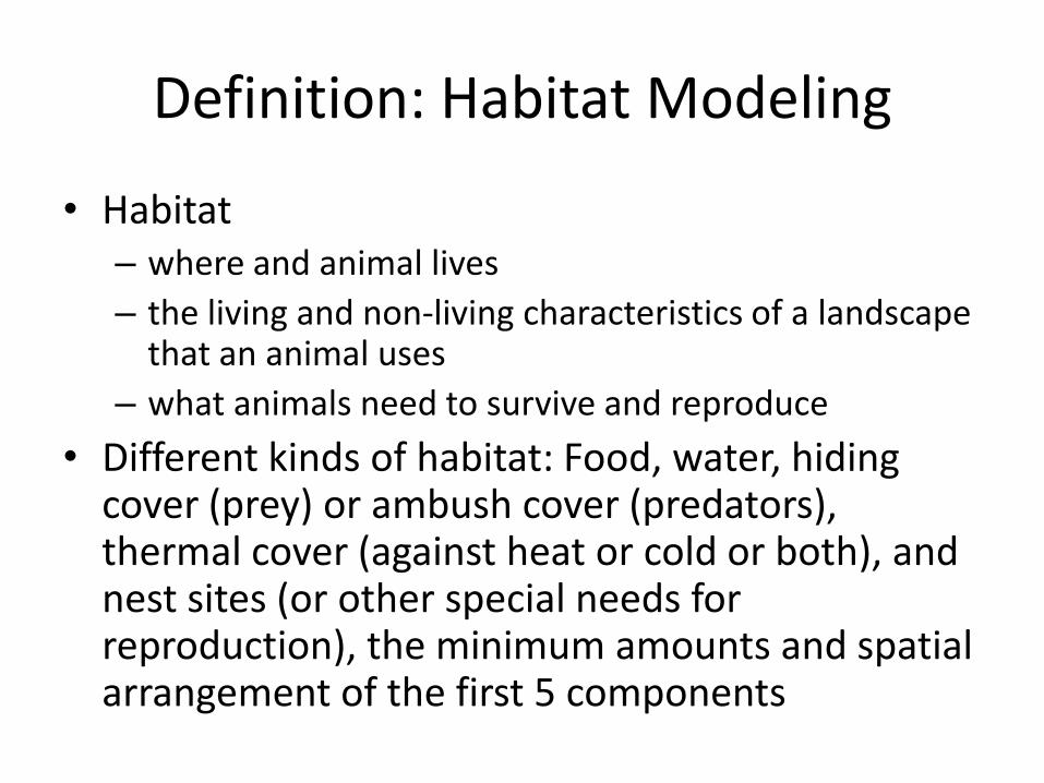
Definition: Habitat Modeling
• Habitat– where and animal lives
– the living and non-living characteristics of a landscape that an animal uses
– what animals need to survive and reproduce
• Different kinds of habitat: Food, water, hiding cover (prey) or ambush cover (predators), thermal cover (against heat or cold or both), and nest sites (or other special needs for reproduction), the minimum amounts and spatial arrangement of the first 5 components
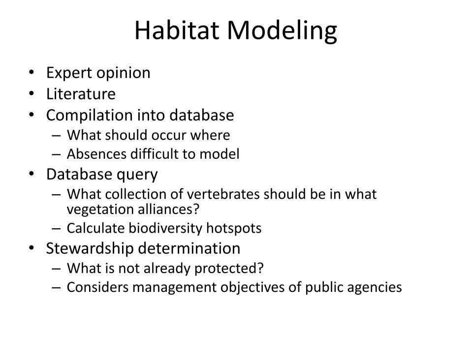
Habitat Modeling
• Expert opinion• Literature• Compilation into database
– What should occur where– Absences difficult to model
• Database query– What collection of vertebrates should be in what
vegetation alliances?– Calculate biodiversity hotspots
• Stewardship determination– What is not already protected?– Considers management objectives of public agencies
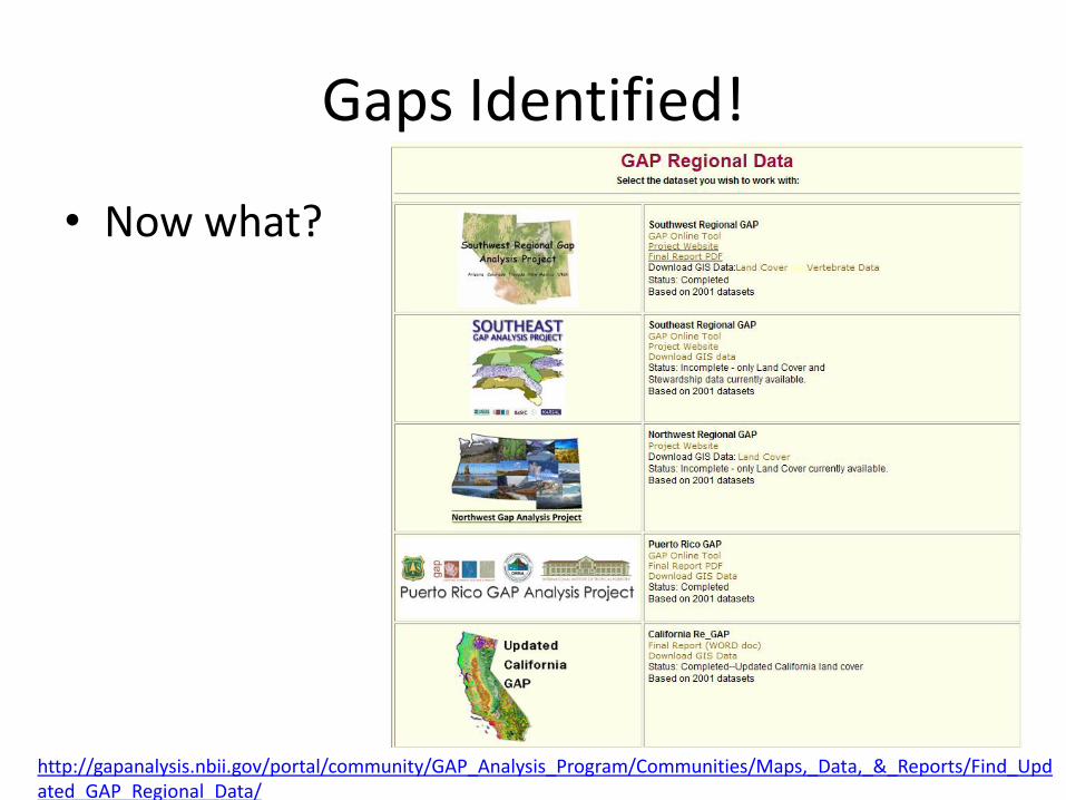
Gaps Identified!
• Now what?
http://gapanalysis.nbii.gov/portal/community/GAP_Analysis_Program/Communities/Maps,_Data,_&_Reports/Find_Updated_GAP_Regional_Data/
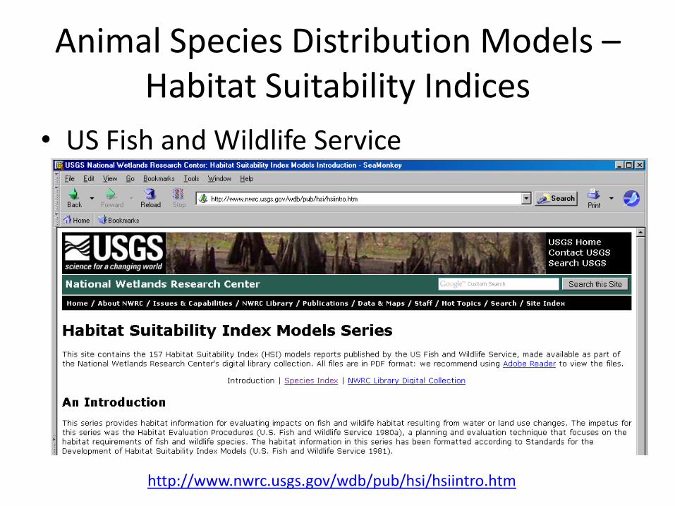
Animal Species Distribution Models –Habitat Suitability Indices
• US Fish and Wildlife Service
http://www.nwrc.usgs.gov/wdb/pub/hsi/hsiintro.htm

Example Habitat Suitability Index: American Alligator (Alligator mississippiensis)
• The American alligator is characteristically a resident of river swamps, lakes, bayous, and marshes of the Gulf and Lower Atlantic Coastal Plains from Texas to North Carolina.
• HSI publications have standard format:– INTRODUCTION
• Distribution and Commercial Importance
• Life History Overview
– HABITAT REQUIREMENTS• food
• Cover
– HABITAT SUITABILITY INDEX (HSI) MODEL• Model Applicability
• Model Description
• Suitability Index (SI) Graphs for Model Variables
• Component Index (CI) Equations and HSI Determination
• Field Use of Model
• Interpreting Model Outputs
– REFERENCES
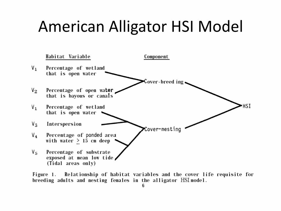
American Alligator HSI Model
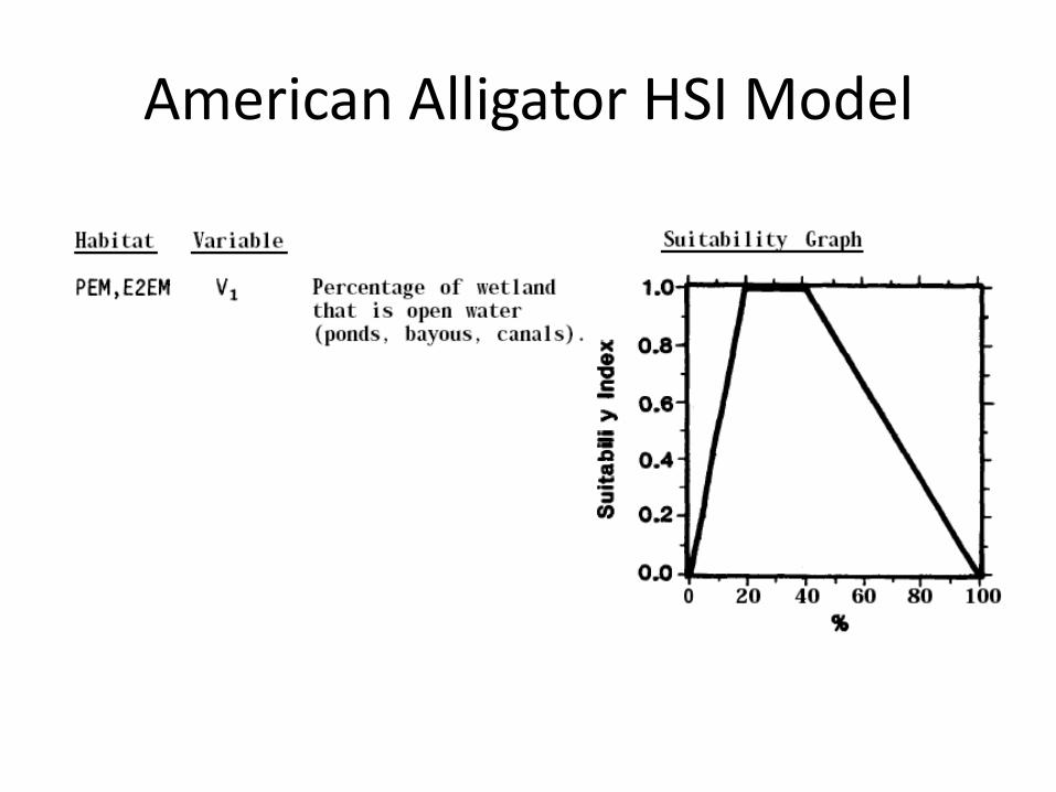
American Alligator HSI Model

American Alligator HSI Model
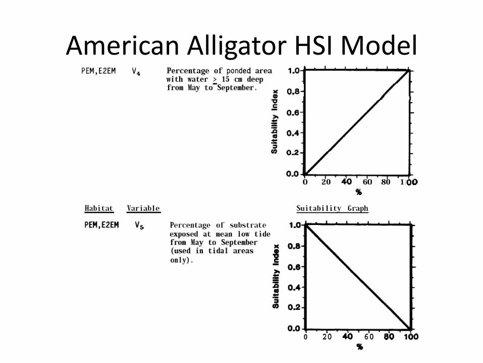
American Alligator HSI Model
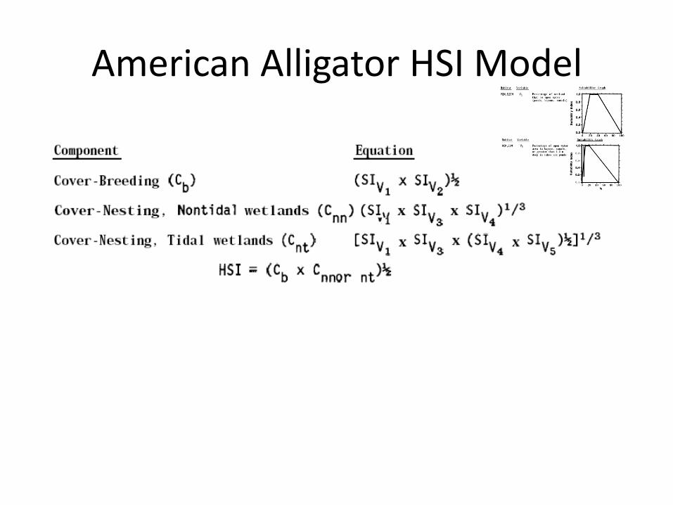
American Alligator HSI Model
American Alligator HSI Model – a Modified Example
• S:\geoglab\Biogeography-Binford
• Copy S:\geoglab\Biogeography-Binford to your computer
• Open the folder and double-click on Alachua_geomorphometry.mxd
• Follow instructions as given by the instructor.
American Alligator HSI Model – a Modified Example
• Develop habitat model– Empirical from alligator sightings
• Randomly select 250 points for model creation• Remaining points are used for model evaluation• Range, regressions
– Deductively• Expert determination of habitat requirements
– Proximity to water (how far?)– Slope (your estimate)– Others?
– Run through model– Test Model
Fundamental Environmental Data
• topographic, hydrologic and solar radiation variables derived from digital elevation data
• “Geomorphometric” data; Terrain attributes
– Slope
– Aspect
– Convexity
– Others
Franklin 1995

Geomorphometric Data: DEM
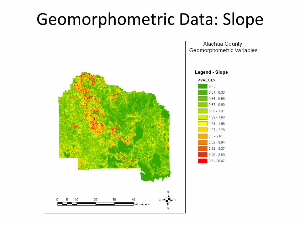
Geomorphometric Data: Slope
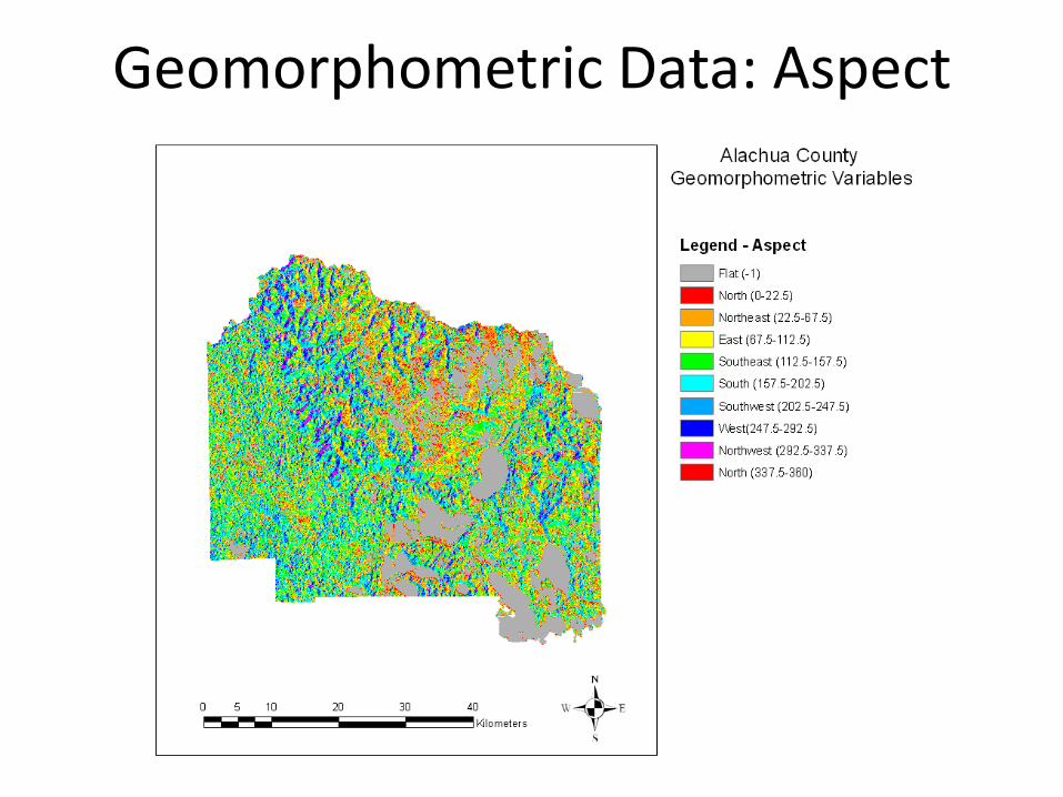
Geomorphometric Data: Aspect
Going Even Further
• Ordination
• Correspondence Analysis
• Multidimensional Scaling
• Logistic Regression (dependent variable is the probability of occurrence).
• Fuzzy classification approaches
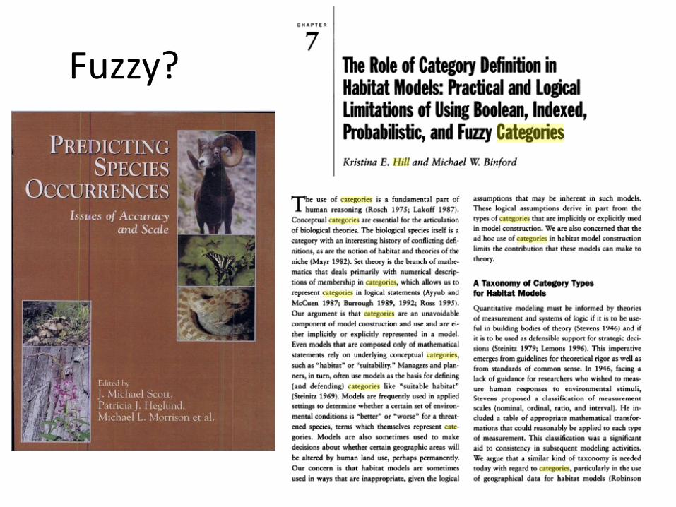
Fuzzy?
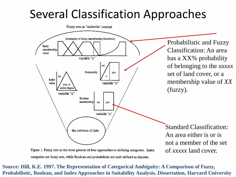
Several Classification Approaches
Source: Hill, K.E. 1997. The Representation of Categorical Ambiguity: A Comparison of Fuzzy,
Probabilistic, Boolean, and Index Approaches in Suitability Analysis. Dissertation, Harvard University
Standard Classification:
An area either is or is
not a member of the set
of xxxxx land cover.
Probabilistic and Fuzzy
Classification: An area
has a XX% probability
of belonging to the xxxxx
set of land cover, or a
membership value of XX
(fuzzy).