GHG Emission Assessment Guideline

Volume I: Soil Carbon and Nitrogen Stock

Assessment in Agricultural Land and

Agroforestry Systems

Field Guide for Practitioners

FEDERAL DEMOCRATIC REPUBLIC OF ETHIOPIA MINISTRY OF AGRICULTURE ADDIS ABABA ETHIOPIA

About the authors Acknowledgements The authors would like to thank the Ministry of Agriculture – Natural Resources Management Directorate – CRGE unit for providing financial assistance and technical support in the development of this guideline. Produced by Echnoserve Consulting December 2014 Front cover photo: Credit: Bayu Nebsu & Tibebu Asefa (Echnoserve)

3 | P a g e

This manual was compiled by Echnoserve PLC for the Ministry of Agriculture as part of its

Executive Entity engagement in the implementation of a CRGE Fast Track Project Entitled

“Technical Assistance and Capacity building on M&E, MRV and long term Investment plan for selected

Agricultural Sector CRGE Fast Track Project Woredas.”

November 2014

Addis Ababa

4 | P a g e

TABLE OF CONTENTS

Acronyms ................................................................................................................................................................. 5

Users of the Manual .............................................................................................................................................. 6

Preface ....................................................................................................................................................................... 7

I. Introduction ................................................................................................................................................... 8

II. Soil Carbon Stock Assessment Methods .............................................................................................. 9

II.1 The Direct Method .................................................................................................................................... 9

ii.2 Indirect methods .................................................................................................................................... 10

III. Steps for the INdirect soil carbon assessment Method .......................................................... 14

IV. Steps for the direct soil carbon assessment Method ............................................................... 25

IV.1 Define and Bound the Measurement Site/Project Area ........................................................ 25

IV.2 Stratify the Area/Landscape ............................................................................................................ 26

IV.3 Determine the Number of Sample Plots ...................................................................................... 27

IV.4 Randomize/locate the Measurement Plots within the target area and strata ............ 28

IV.5 Decide on the Shape and Size of the Sample plot ..................................................................... 30

IV.5 Determining Measurement Frequency ........................................................................................ 30

IV.6 Field Measurement of SOC ................................................................................................................ 31

References ............................................................................................................................................................ 37

Glossary of Terms .............................................................................................................................................. 39

Annex 1: Key Features of the Agro-ecological zones ........................................................................... 40

Annex 2: Default Emission and Parameter values relevant to calculate N2O emission ......... 41

Annex 3: Combustion factor values for fires in a range of vegetation types (From Table 2.6,

2006 IPCC Guidelines for National Greenhouse Gas Inventories) .................................................. 42

Annex 4: Above Ground Biomass Field Inventory From .................................................................... 43

Annex 5: A section of the interface of the online tool for estimating number of plots ........... 44

Annex 6: Data collection tool for EX-ACT: Annual Production System ......................................... 45

Annex 7: Data collection tool for EX-ACT: Inputs & Investments used for agricultural

production ............................................................................................................................................................ 46

5 | P a g e

ACRONYMS

GHG Greenhouse Gas

GPG Good Practice Guide

GPS Geographical Positioning System

IPCC Intergovernmental Panel on Climate Change

LULUCF Land Use, Land Use Cover Change and Forestry

MRV Measurement, Reporting and Verifications

NAMAs Nationally Appropriate Mitigation Actions

PDD Project Design Document

PIN Project Idea Note

SOC Soil Organic Carbon

SIC Soil Inorganic Carbon

UNFCCC United Nations Framework Convention on Climate Change

6 | P a g e

USERS OF THE MANUAL

This manual is compiled to serve as a field guide for practitioners, who conduct soil Carbon and

Nitrogen stock assessment in different land use types in Ethiopian Agricultural systems. The

manual can also be used in similar landscapes in the tropics. Besides, academic institutions and

researchers may find it as a useful reference material to offer short-term courses on soil carbon and

nitrogen stock assessment for students and practitioners.

7 | P a g e

PREFACE

The manual presents roles of soil and agricultural practices in climate change mitigation, steps to be

followed to collect relevant field data the field and computational procedures for accurate soil

carbon and nitrogen stocks estimations in different agricultural systems and practices.

Relevant materials on climate change, soil carbon and nitrogen stock assessment including

sourcebooks, guidelines, procedures, etc. were consulted to enrich the manual. The manual is

expected to provide practical guidance for practitioners who would like to conduct soil carbon and

nitrogen stock assessments for emission trading, and other research activities in Ethiopia.

The manual is specifically designed to capture the local context in Ethiopia, based on its unique

landscape and vegetation. The soli carbon and nitrogen stock assessment methods and techniques

described in this manual are consistent with the IPCC (2003) GPG and (2006) GPG for Land Use,

Land-Use Change and Forestry. The manual, however, shouldn’t be considered as an exhaustive

document. Users are advised to consult relevant references, IPPC guidelines, and the like for further

details

I. INTRODUCTION

Soils are among the largest terrestrial reservoirs of carbon and hold potential for expanded Carbon

sequestration. Soils sink carbon and release to the atmosphere when the equilibrium (i.e. inflow

and outflow) carbon content is disrupted due to human actions such as land use change,

precipitation, temperature, etc. During this process, soil may act as a carbon source or a carbon sink

according to the ratios between inflows and outflows. Thus, they are critically important in

determining global carbon cycle dynamics and can provide a potential way to reduce atmospheric

concentration of carbon dioxide.

Soil carbon pool comprises of Soil Organic Carbon (SOC) and Soil Inorganic Carbon (SIC). The SOC

pool includes highly active humus to relatively inert charcoal Carbon. The SIC pool includes

elemental Carbon and carbonate minerals (e.g. gypsum, calcite, dolomite, aragonite and siderite).

The SOC pool represents a dynamic balance between gains and losses. The amount changes over

time depending on photosynthetic Carbon added and the rate of its decay. Under undisturbed

natural conditions, inputs of carbon from litter fall and root biomass are cycled by output through

erosion, organic matter decomposition, and leaching. Soils in tropical regions are low in SOC

particularly those under the influence of arid, semiarid and sub-humid climates and this are a major

factor contributing to their poor productivity. Therefore, proper management of SOC is important

for sustaining soil productivity and ensuring food security as well as protection from land

degradation.

9 | P a g e

II. SOIL CARBON STOCK ASSESSMENT METHODS

Soil carbon assessment in different parts of the world requires methods that are appropriate to the

circumstances. Many different methods have been tested in a number of countries, but effort is

required to ensure that the methods are comparable. Furthermore, for carbon projects, credible

and cost-effective techniques of monitoring changes in soil carbon are required. Soil carbon

assessment methods can be broadly classified into direct and indirect methods depending on

whether carbon content in soil samples is directly measured or inferred through a proxy variable.

There are several factors, which should be taken into consideration when selecting a method for the

determination of soil organic carbon. These factors include the ease of use, health and safety

concerns, cost, sample throughput, and comparability to standard reference methods. These factors

are a concern for both the sample preparation and sample quantitation phases of SOC

determinations.

II.1 THE DIRECT METHOD

The direct soil organic carbon assessment entails collecting soil samples in the field and analyzing

them in the laboratory using combustion techniques. The direct methods of measuring carbon in

soils in LULUCF projects are based on commonly accepted principles of soil sampling, and

ecological surveys. The methods, however, haven’t been universally applied to all projects, and not

standardized. In the specific case of soils, the depth to which soil carbon pool should be measured

and monitored may vary according to project type, site conditions, species, and expected depth at

which change will take place. Because the highest concentration of soil organic carbon is in the

upper layer of the soil, and it decreases exponentially with increasing depth. The IPCC (2006)

recommends the sampling of the top 0.3-m depth of soil for SOC stock measurement or estimation

since changes in SOC stock due to land-use change or management are primarily confined to the top

0.1- or 0.3-m depths in most soils. In other words, this is the depth where typically the changes in

soil carbon pool are likely to be fast enough to be detected during the project period. Direct

methods are more precise and accurate but also more time and labor intensive, involves technically

challenging field sampling process as well as very expensive. Most assessments typically involve a

combination of direct and indirect techniques. Some in situ soil carbon analytical methods are being

developed with the objective of offering increased accuracy, precision, and cost-effectiveness over

conventional ex situ methods. The in situ soil carbon analytical methods include mid-infrared (IR)

10 | P a g e

spectroscopy, near-IR spectroscopy, laser-induced breakdown spectroscopy (LIBS), and inelastic

neutron scattering (INS). While LIBS and INS technologies are still in their infancy, IR spectroscopy

has proven valuable in developing soil spectral libraries and for rapid characterization of soil

properties for soil quality monitoring and other agricultural applications in developed and

developing countries.

II.2 INDIRECT METHODS

The direct method, though more precise and accurate, is quite laborious and very expensive. The

indirect methods, which comprise the use of in situ analytical methods, and the use of

biogeochemical models, reduce cost of soil carbon monitoring. Indirect estimation of soil organic

carbon changes over large areas using simulation models has become increasingly important.

Indirect methods are needed to fill knowledge gaps about the biogeochemical processes involved in

soil carbon sequestration. One of the more important indirect methods involves the use of

simulation models that project changes in soil organic carbon under varying climate, soil, and

management conditions. Although simulation models can have limited accuracy, particularly in the

context of developing countries in which land resources data are scarce, they are a cost-effective

means of estimating GHG emissions in space and time under a wide range of biophysical and

agricultural management conditions. The data can be particularly useful in scaling-up site-specific

information to larger scales of magnitude.

A. Options for Estimating Soil Organic Carbon Stock

Under the UNFCCC, countries must estimate and report GHG emissions and removals, including

changes in carbon stocks in all five pools (above- and belowground biomass, dead wood, litter and

soil carbon) and associated emissions and removals from land use, land-use change and forestry

(LULUCF) activities according to the Good Practice Guide (GPG). Measurement, Reporting and

Verification (MRV) gives opportunities to developing countries to claim financial, technical and

capacity building supports from developed countries to implement their Nationally Appropriate

Mitigation Actions (NAMAs). Understanding these benefits, a growing number of developing

countries have drafted, adopted and, in some cases, started implementing national climate action

plans. However, lack of a robust method of measuring NAMAs and the technical gaps are serious

11 | P a g e

challenges in developing countries. The IPCC has developed standard methods for estimating soil

organic carbon stocks and stock changes. These methods are characterized by flexibility, ranging

from the Tier 1default method prescribed by IPCC with fixed default values, to methods that

incorporate local information to estimate carbon stock changes at Tier 2 level, and to more

advanced modeling and measurement based networks at Tier 3 level. The “Tiers” represent

increasing level of data requirement and analytical complexity. Despite differences in approach

among the three Tiers, all tiers have common adherence to IPCC good practice concepts of

transparency, completeness, consistency, comparability and accuracy. Soil has much more variability

than vegetation and therefore needs more sampling effort, which sometimes may exceed the

benefits expected from the increase in stock (IPCC, 2003). Therefore developing locally calibrated

models that can use easily collected data can minimize the cost of demonstrating a change in soil

organic carbon stock.

Tier 1: methods are designed to be the simplest to use, for which equations and default

parameter values (e.g., emission and stock change factors) are provided in this volume. It

requires no new data collection to generate estimates of forest biomass. Default values,

which are available globally such as deforestation rates, agricultural production statistics,

and global land cover maps, fertilizer use, livestock population data, etc. can be obtained

from the IPCC emission factor database. Its estimation thus provides limited resolution of

how soil carbon varies sub-nationally and has a large error range for growing stock in

developing countries. Tier 1 has essentially no data collection needs beyond consulting

the IPCC table and Emission Factor Data Base (EFDB), corresponding to broad continental

forest types.

Tier 2: can use the same methodological approach as Tier 1 but applies emission and stock

change factors that are based on country- or region-specific data, for the most important

land-use or livestock categories. Country-defined emission factors are more appropriate

for the climatic regions, land-use systems and livestock categories in that country. Higher

temporal and spatial resolution and more disaggregated activity data are typically used in

Tier 2 to correspond with country-defined coefficients for specific regions and specialized

land-use or livestock categories.

Tier 3: higher order methods are used including models and inventory measurement systems

tailored to address national circumstances, repeated over time, and driven by high-

12 | P a g e

resolution activity data and disaggregated at sub-national level. These higher order

methods provide estimates of greater certainty than lower tiers. Such systems may

include comprehensive field sampling repeated at regular time intervals and/or GIS-

based systems of age, class/production data, soils data, and land-use and management

activity data, integrating several types of monitoring. Pieces of land where a land-use

change occurs can usually be tracked over time, at least statistically. In most cases these

systems have a climate dependency, and thus provide source estimates with inter-annual

variability. Detailed disaggregation of livestock population according to animal type, age,

body weight etc., can be used. Models should undergo quality checks, audits, and

validations and be thoroughly documented. The tier 3 approach requires long term

commitments of resources and personnel, generally involving the establishment of a

permanent organization to house the program. It is expensive in the developing countries

context.

The tiers should be selected on the basis of goal, cost, and significance of the target source/sink,

available data and analytical capability. If Tiers 1 or 2 is used both for the reference period and for

future monitoring of emissions from soils, the error margin may be so great that the amount of

emissions to be claimed and traded could be small make the effort not worthwhile. The IPCC

recommends that it is good practice to use higher tiers for measurement of significant

sources/sinks.

13 | P a g e

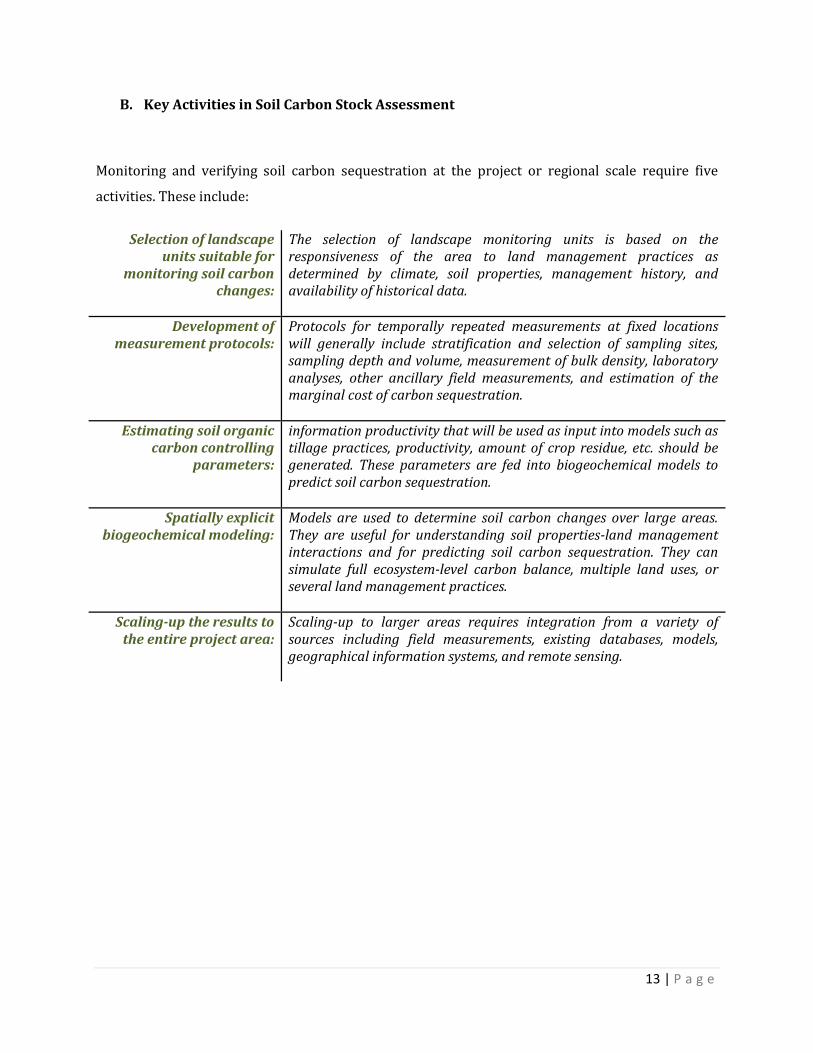
B. Key Activities in Soil Carbon Stock Assessment

Monitoring and verifying soil carbon sequestration at the project or regional scale require five

activities. These include:

Selection of landscape

units suitable for monitoring soil carbon

changes:

The selection of landscape monitoring units is based on the responsiveness of the area to land management practices as determined by climate, soil properties, management history, and availability of historical data.

Development of measurement protocols:

Protocols for temporally repeated measurements at fixed locations will generally include stratification and selection of sampling sites, sampling depth and volume, measurement of bulk density, laboratory analyses, other ancillary field measurements, and estimation of the marginal cost of carbon sequestration.

Estimating soil organic carbon controlling

parameters:

information productivity that will be used as input into models such as tillage practices, productivity, amount of crop residue, etc. should be generated. These parameters are fed into biogeochemical models to predict soil carbon sequestration.

Spatially explicit biogeochemical modeling:

Models are used to determine soil carbon changes over large areas. They are useful for understanding soil properties-land management interactions and for predicting soil carbon sequestration. They can simulate full ecosystem-level carbon balance, multiple land uses, or several land management practices.

Scaling-up the results to the entire project area:

Scaling-up to larger areas requires integration from a variety of sources including field measurements, existing databases, models, geographical information systems, and remote sensing.

14 | P a g e

III. STEPS FOR THE INDIRECT SOIL CARBON ASSESSMENT METHOD

3.1 Overview of Soil Carbon

Cropland management modifies soil C stocks to varying degrees depending on how specific

practices influence C input and output from the soil system. The main management practices that

affect soil C stocks in croplands are the type of residue management, tillage management, fertilizer

management (both mineral fertilizers and organic amendments), choice of crop and intensity of

cropping management (e.g., continuous cropping versus cropping rotations with periods of bare

fallow), irrigation management, and mixed systems with cropping and pasture or hay in rotating

sequences. In addition, drainage and cultivation of organic soils reduces soil C stocks.

The total change in soil C stocks for Cropland is estimated using Equation 2.24.

EQUATION 2.24: ANNUAL CHANGE IN CARBON STOCKS IN SOILS

ΔC soils = ΔC mineral – L organic + ΔC Inorganic ----------------------------------------------------------------------------- (eq. 24).

Where:

ΔC Soils = annual change in carbon stocks in soils, tonnes C yr-1

ΔC Mineral = annual change in organic carbon stocks in mineral soils, tonnes C yr-1

L Organic = annual loss of carbon from drained organic soils, tonnes C yr-1

ΔC Inorganic = annual change in inorganic carbon stocks from soils, tonnes C yr-1 (assumed to be 0

unless using a Tier 3 approach)

For Tier 1 and 2 methods, soil organic C stocks for mineral soils are computed to a default depth of

30 cm.

3.2 Mineral Soils

3.2.1Choice of Methods

15 | P a g e

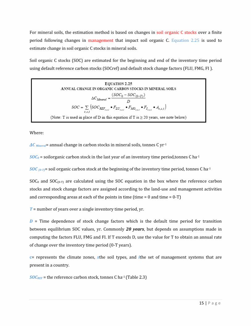
For mineral soils, the estimation method is based on changes in soil organic C stocks over a finite

period following changes in management that impact soil organic C. Equation 2.25 is used to

estimate change in soil organic C stocks in mineral soils.

Soil organic C stocks (SOC) are estimated for the beginning and end of the inventory time period

using default reference carbon stocks (SOCref) and default stock change factors (FLU, FMG, FI ).

Where:

ΔC Mineral= annual change in carbon stocks in mineral soils, tonnes C yr-1

SOC0 = soilorganic carbon stock in the last year of an inventory time period,tonnes C ha-1

SOC (0-T)= soil organic carbon stock at the beginning of the inventory time period, tonnes C ha-1

SOC0 and SOC(0-T) are calculated using the SOC equation in the box where the reference carbon

stocks and stock change factors are assigned according to the land-use and management activities

and corresponding areas at each of the points in time (time = 0 and time = 0-T)

T = number of years over a single inventory time period, yr.

D = Time dependence of stock change factors which is the default time period for transition

between equilibrium SOC values, yr. Commonly 20 years, but depends on assumptions made in

computing the factors FLU, FMG and FI. If T exceeds D, use the value for T to obtain an annual rate

of change over the inventory time period (0-T years).

c= represents the climate zones, sthe soil types, and ithe set of management systems that are

present in a country.

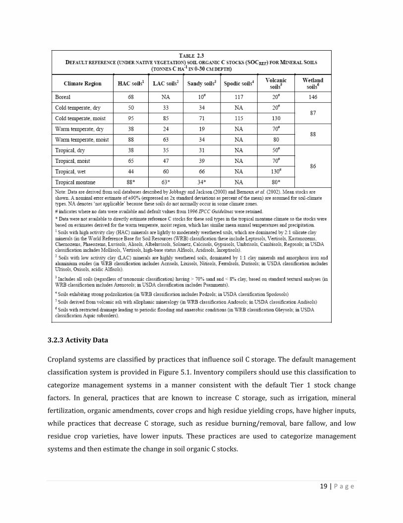
SOCREF = the reference carbon stock, tonnes C ha-1 (Table 2.3)

16 | P a g e

FLU = stock change factor for land-use systems or sub-system for a particular land-use,

dimensionless

[Note: FND is substituted for FLU in forest soil C calculation to estimate the influence of natural

disturbance regimes.]

FMG = stock change factor for management regime, dimensionless

FI = stock change factor for input of organic matter, dimensionless

A = land area of the stratum being estimated, ha.

N.B: All land in the stratum should have common biophysical conditions (i.e., climate and soil type)

and management history over the inventory time period to be treated together for analytical

purposes.

3.2.2 Emission Factors

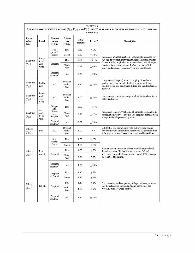
Table 5.5 provides Tier 1 approach default stock change factors for land use (FLU), input (FI) and

management (FMG). The method and studies that were used to derive the default stock change

factors are provided in Annex 5A.1 and References. The default time period for stock changes (D) is

20 years and management practice is assumed to influence stocks to a depth of 30 cm, which is also

the depth for the reference soil C stocks in Table 2.3.

17 | P a g e

18 | P a g e

19 | P a g e

3.2.3 Activity Data

Cropland systems are classified by practices that influence soil C storage. The default management

classification system is provided in Figure 5.1. Inventory compilers should use this classification to

categorize management systems in a manner consistent with the default Tier 1 stock change

factors. In general, practices that are known to increase C storage, such as irrigation, mineral

fertilization, organic amendments, cover crops and high residue yielding crops, have higher inputs,

while practices that decrease C storage, such as residue burning/removal, bare fallow, and low

residue crop varieties, have lower inputs. These practices are used to categorize management

systems and then estimate the change in soil organic C stocks.

20 | P a g e

Practices should not be considered that are used in less than 1/3 of a given cropping sequence (i.e.,

crop rotation), which is consistent with the classification of experimental data used to estimate the

default stock change factors. Rice production, perennial croplands, and set-aside lands (i.e., lands

removed from production) are considered unique management systems (see below).

Each of the annual cropping systems (low input, medium input, high input, and high input

w/organic amendment) are further subdivided based on tillage management. Tillage practices are

divided into no-till (direct seeding without primary tillage and only minimal soil disturbance in the

seeding zone; herbicides are typically used for weed control), reduced tillage (primary and/or

secondary tillage but with reduced soil disturbance that is usually shallow and without full soil

inversion; normally leaves surface with >30% coverage by residues at planting) and full tillage

(substantial soil disturbance with full inversion and/or frequent, within year tillage operations,

while leaving <30% of the surface covered by residues at the time of planting). It is good practice

only to consider reduced and no-till if they are used continuously (every year) because even an

occasional pass with a full tillage implement will significantly reduce the soil organic C storage

expected under the reduced or no-till regimes.

The main types of land-use activity data are: i) aggregate statistics (Approach 1), ii) data with

explicit information on land-use conversions but without specific geo-referencing (Approach 2), or

iii) data with explicit information on land-use conversions and geo-referencing (Approach 3), such

as land-use and management inventories making up a statistically-based sample of a country’s land

area (see Chapter 3 for discussion of approaches). At a minimum, globally available land-use and

crop production statistics, such as FAO databases(http://faostat.fao.org/), provide annual

compilations of total land area by major land-uses, select management data (e.g., irrigated vs. non-

irrigated cropland), land area in ‘perennial’ crops (i.e., vineyards, perennial herbaceous crops, and

tree-based crops such as orchards) and annual crops (e.g., wheat, rice, maize, sorghum, etc.). FAO

databases would be an example of aggregate data (Approach 1).

Management activity data supplement the land-use data, providing information to classify

management systems, such as crop types and rotations, tillage practices, irrigation, manure

application, residue management, etc.

21 | P a g e

These data can also be aggregate statistics (Approach 1) or information on explicit management

changes

(Approach 2 or 3). Where possible, it is good practice to determine the specific management

practices for land areas associated with cropping systems (e.g., rotations and tillage practice),

rather than only area by crop.

Remote sensing data are a valuable resource for land-use and management activity data, and

potentially, expert knowledge is another source of information for cropping practices. It is good

practice to elicit expert knowledge using methods provided in Volume 1, Chapter 2 (eliciting expert

knowledge).

National land-use and resource inventories, based on repeated surveys of the same locations,

constitute activity data gathered using Approach 2 or 3, and have some advantages over aggregated

land-use and cropland management data (Approach 1). Time series data can be more readily

associated with a particular cropping system (i.e., combination of crop type and management over a

series of years), and the soil type can be determined by sampling or by referencing the location to a

suitable soil map. Inventory points that are selected based on an appropriate statistical design also

enable estimates of the variability associated with activity data, which can be used as part of a

formal uncertainty analysis. An example of a survey using Approach 3 is theNational Resource

Inventory in the U.S.

Activity data require additional in-country information to stratify areas by climate and soil types. If

such information has not already been compiled, an initial approach would be to overlay available

land cover/land-use maps (of national origin or from global datasets such as IGBP_DIS) with soil

and climate maps of national origin or global sources, such as the FAO Soils Map of the World and

climate data from the United Nations Environmental Program. A detailed description of the default

climate and soil classification schemes is provided in Chapter 3, Annex 3A.5. The soil classification

is based on soil taxonomic description and textural data, while climate regions are based on mean

annual temperatures and precipitation, elevation, occurrence of frost, and potential

evapotranspiration.

3.2.4 Calculation Steps

The steps for estimating SOC0 and SOC (0-T) and net soil C stock change per ha for Cropland

Remaining Cropland on mineral soils are as follows:

22 | P a g e

Step 1: Organize data into inventory time periods based on the years in which activity data were

collected (e.g., 1990 to 1995, 1995 to 2000, etc.)

Step 2: Determine the amount Cropland Remaining Cropland by mineral soil types and climate

regions in the country at the beginning of the first inventory time period. The first year of the

inventory time period will depend on the time step of the activity data (0-T; e.g., 5, 10 or 20 years

ago).

Step 3: Classify each Cropland into the appropriate management system using Figure 5.1.

Step 4: Assign a native reference C stock values (SOCREF) from Table 2.3 based on climate and soil

type.

Step 5: Assign a land-use factor (FLU), management factor (FMG) and C input levels (FI) to each

Cropland based on the management classification (Step 2). Values for FLU, FMG and FI are given in

Table 5.5.

Step 6: Multiply the factors (FLU, FMG, FI ) by the reference soil C stock (SOCREF) to estimate an

‘initial’ soil organic C stock (SOC (0-T)) for the inventory time period.

Step 7: Estimate the final soil organic C stock (SOC0) by repeating Steps 1 to 5 using the same

native reference C stock (SOCREF), but with land-use, management and input factors that represent

conditions for each cropland in the last (year 0) inventory year.

Step 8: Estimate the average annual change in soil organic C stocks for Cropland Remaining

Cropland (ΔC Mineral) by subtracting the ‘initial’ soil organic C stock (SOC (0-T)) from the final soil

organic C stock (SOC0), and then dividing by the time dependence of the stock change factors (i.e.,

20 years using the default factors). If an inventory time period is greater than 20 years, then divide

by the difference in the initial and final year of the time period.

Step 9: Repeat steps 2 to 8 if there are additional inventory time periods (e.g., 1990 to 2000, 2001

to 2010, etc.). A numerical example is given below for Cropland Remaining Cropland on mineral

soils, using Equation 2.25 and default reference C stocks (Table 2.3) and stock change factors (Table

5.5).

23 | P a g e

3.3 Organic Soils

3.3.1Choice of Methods

Equation 2.26 is used to estimate C stock change in organic soils (e.g., peat-derived, Histosols). The

basic methodology is to stratify cultivated organic soils by climate region and assign a climate-

specific annual C loss rate. Land areas are multiplied by the emission factor and then summed up to

estimate annual C emissions.

Where:

L Organic = annual carbon loss from drained organic soils, tonnes C yr-1

A = land area of drained organic soils in climate type c, ha

Note: A is the same area (Fos) used to estimate N2O emissions in Chapter 11, Equations 11.1 and 11.2

EF = emission factor for climate type c, tonnes C ha-1 yr-1

3.3.2 Emission Factors

Default emission factors are provided in Table 5.6 for cultivated organic soils. Assignment of

emission factors for perennial tree systems, such as fruit trees that are classified as Cropland, may

24 | P a g e

be based on the factors for cultivated organic soils in Table 5.6 or forest management of organic

soils (see Chapter 4). Shallower drainage will lead to emissions more similar to forest management,

while deeper drainage of perennial tree systems will generate emissions more similar to annual

cropping systems.

3.3.3 Activity Data

In contrast to the mineral soil method, croplands on organic soils are not classified into

management systems under the assumption that drainage associated with all types of management

for crops stimulates oxidation of organic matter previously built up under a largely anoxic

environment. However, in order to apply the method described in Section 2.3.3.1 (Chapter 2),

croplands do need to be stratified by climate region and soil type (see Chapter 3, Annex 3A.5 for

guidance on soil and climate classifications).

Similar databases and approaches as those outlined for Mineral Soils in the Tier 1 discussion can be

used for deriving area estimates. The land area with organic soils that are managed for Cropland

can be determined using an overlay of a land-use map on climate and soils maps. Country-specific

data on drainage projects combined with land-use surveys can be used to obtain a more refined

estimate of the relevant areas.

3.3.4 Calculation Steps

The steps for estimating the loss of soil C from drained organic soils are as follows:

Step 1: Organize data into inventory time periods based on the years in which activity data were collected (e.g., 1990 to 1995, 1995 to 2000, etc.)

Step 2: Determine the amount of Cropland Remaining Cropland on organic soils for the last year of each inventory time period.

Step 3: Assign the appropriate emission factor (EF) for annual losses of CO2 based on climate (from Table 5.6).

Step 4: Estimate total emissions by summing the product of area (A) multiplied by the emission factor (EF) for all climate zones.

Step 5: Repeat for additional inventory time periods. A numerical example is given below for Cropland Remaining Cropland on drained organic soils, using Equation 2.26 and default emission factors (Table 5.6).

25 | P a g e

IV. STEPS FOR THE DIRECT SOIL CARBON ASSESSMENT METHOD

Carbon stocks and greenhouse gas emissions should be measured and reported in compliance with

the UNFCCC reporting principles of transparency, consistency, comparability, completeness, and

accuracy. The majority of the non-Annex I Parties uses the IPCC default assumption that there are

no changes in soil carbon. Given that soil carbon is a significant carbon pool, it is critical to estimate

stocks and changes, using higher tier methods in line with IPCC GPG for LULUCF. The use of a

higher tier method improves estimates of carbon emissions and removals compared with the

default method. Several steps are required to estimate changes in soil organic carbon stocks within

a project area over time. A hybrid approach (Tier-3) involving a combination of approaches (e.g.,

combining modeling with on-site sampling and independent verification) is preferable in terms of

improved accuracy of carbon stock estimation. The on-site soil carbon stock assessment involves

the following key steps:

IV.1 DEFINE AND BOUND THE MEASUREMENT SITE/PROJECT AREA

Given the inherent high spatial variability of soil organic carbon, an accurate quantification and

monitoring of SOC stocks and stock changes is a complex task even in relatively homogeneous

ecosystems. Such feature is further exacerbated in the case of smallholder environments by the

existence of multiple land use activities occurring at various management intensities. Moreover,

sources of uncertainty and suitable levels of precision and accuracy differ when working at the

landscape scale as opposed to the farm scale for the reason that biogeochemical processes affecting

SOC dynamics operate and interact at different spatial scales.

The measurement sites are typically large enough to capture variation in conditions at the

landscape scale (e.g. valley bottoms, slopes, ridge-tops) and can be replicated at different scales,

within projects, watersheds, administrative boundaries, countries, or even continents.

Before proceeding to the next steps of carbon stock assessment, it is important to delineate the

project boundary, with active participation of relevant stakeholders including communities living in

and around the project area. This process is important to know the actual size of the project and is

crucial for the sustainability of the carbon stock. When the boundary is agreed among stakeholders,

coordinates should be recorded using Global Positioning System (GPS). The GPS data will be later

transferred into computer in order to draw the base map of the project and estimate the area. The

26 | P a g e

Arc GIS software would be used to distribute and locate sample plots on the base map. The software

also generates coordinates of each sample plot, which is later used to locate the plots on the ground

during the actual carbon stock assessment.

IV.2 STRATIFY THE AREA/LANDSCAPE

Stratification refers to the division of any heterogeneous landscape into distinct sub-sections

(strata) based on some common grouping factor. In order to facilitate fieldwork and increase the

accuracy and precision of measuring and estimating carbon, it is useful to divide the project area

into sub-populations or “strata” that form relatively homogenous units. If stratification leads to no,

or minimal, change in costs, then it should not be undertaken.

Stratification of the landscape/watershed into more or less homogenous clusters or land use

systems should be on the basis of parameters such as climate (rainfall, temperature), topography,

land use, land management, land cover, soil type, availability of data, etc. Stratifying on too many

variables can rapidly become un-manageable in terms of the number of strata produced and in

practice it is often adequate to stratify on at most several major ecological zones. The initial

stratification should be conducted in a hierarchical order whereby the factor that exerts the

strongest influence on SOC stocks is ranked first, and other factors with less influence on SOC are

subsequently assigned (e.g. a classical ranking approach might be climate, soil texture, land cover

and land use management, etc.).

In Ethiopia context, Agro-ecological zones are considered suitable for stratification as they create

homogenous stratum in terms of bio-physical conditions, including climate, terrain, soil, vegetation.

On this basis, there are five AEZs, namely; Tepid to cool sub-humid mid highlands, Hot to warm

humid lowlands, Tepid to cool humid mid highlands, Tepid to cool moist mid highlands, and Tepid to

cool sub-moist mid highlands. A description of the characteristics of the AEZs is presented as annex

1.

27 | P a g e

IV.3 DETERMINE THE NUMBER OF SAMPLE PLOTS

Once the strata’s are identified and agreed on, the number of sample plots required in each stratum

must be determined. The decision on the number of plots depends on the required level of

accuracy, logistics, manpower, cost and the length of the monitoring interval. Due to the

heterogeneity of SOC distribution, the number of samples required to accurately assess SOC stocks

at scales suitable for carbon trading is high. When designing sampling campaigns, taking into

account the factors influencing SOC distribution, such as soil type, land-use, climate, and vegetation

will help to optimize sampling depths and numbers, ensuring that samples accurately reflect the

distribution of SOC at the site.

Optimal size does not necessarily guarantee the desired precision of carbon estimate unless it is

complemented with a proper unbiased sampling design. The number of plots depends on the

variation in soil carbon levels, the required level of accuracy and the length of the monitoring

interval. The number of plots required to measure carbon stocks is often within a precision level of

±10% of the mean SOC stocks at 95% confidence level. In addition to the precision level, the

sampling calculator and the equation require data on average carbon stock of each stratum,

estimate of standard deviation and variance. The following equation can be used to calculate the

number of sample plots. Furthermore, it is possible to use the “Winrock Terrestrial Sampling

Calculator” tool to find the number of sample plots in each stratum. A section of this web-based tool

is presented as presented annex 5. The number of samples to be measured in each stratum should

be determined as a proportion of the area and the variance observed for that particular stratum. It

is assumed that the above parameters are known from the project set up, pre-project estimates (e.g.

results from a pilot-study) or literature data. A training exercise for technicians can generate these

data.

Where: N=Number of sample plots in the project area Ni=Number of sample plots in stratum i A=the total project area in ha Ai= size of each stratum i; ha APi=sample plot size (constant for all strata); ha

28 | P a g e

Where:

n = sample size (total number of sample plots required) in the project area i = 1, 2, 3, … L project strata sti = standard deviation for each stratum i; dimensionless

E1 = allowable error of the estimated quantity Q Q1 = approximate average value of the estimated quantity Q, (e.g. aboveground wood volume

per hectare); e.g. m3

ha-1

p = desired level of precision (e.g. 10%); dimensionless α = 1-α is probability that the estimate of the mean is within the error bound E zα/2= value of the statistic z (embedded in Excel as: inverse of standard normal probability

cumulative distribution), for e.g. 1-α = 0.05 (implying a 95% confidence level) zα/2

=1.9599 It is possible to reasonably modify (e.g. increase or decrease) the sample size after the pre-sampling

or first monitoring event based on the actual variation of the carbon stock changes determined

from taking the initial samples.

IV.4 RANDOMIZE/LOCATE THE MEASUREMENT PLOTS WITHIN THE TARGET AREA AND

STRATA

After the quantity of sample plots are identified, a sampling grid could be used to systematically

layout the sample plots on the map (aerial photos or topographic map) of the project. This is

important to provide unbiased estimates of carbon stocks and other parameters such as yield,

organic and inorganic fertilizers application, livestock type and number, residue management, etc.

The distance between grids depends on the number of sample plots and each sample point on the

grid represents an area corresponding to the size of the grid cell of the sample layout. For example,

29 | P a g e

if the distance between square grids is 1km, each sample point represents an area of 1km x 1km=

10ha. Thus, if 15 plots fall within a stratum, the interest of the area estimate will be 15 x 10ha=

150ha.

The number of plots to be characterized per strata depends on the level of variability within strata

in the target area, the size of the stratum, required levels of precision and resource availability.

Viewing the site on satellite images or using Google Earth can provide information on terrain and

vegetation type, road access, population center, etc. To avoid subjective choice of plot locations

(plot centers, plot reference points, movement of plot centers to more “convenient” positions), the

permanent sample plots must be located randomly or systematically with a random start within

each identified stratum. Random location of plots can be accomplished in one of two ways:

Locate plots systematically with a random start. In this case the plots are located using a

systematic method-usually on a grid, with the location of the first points on the grid

determined randomly. This must be undertaken prior to field work, with the plot locations

specified on a map or aerial photos, and locations specified either as distance and direction

from a known point or as a GPS coordinate.

Locate individual plots randomly, using a randomization procedure in a GIS to specify the

coordinates of each plot.

If the stratum consists of sites that are geographically separated, then the plots to be allocated to

each site should be in proportion of the site area to the total stratum area with rounding of the

fractions. For example, if one stratum consists of three geographically separated sites, then it is

proposed to:

Divide the total stratum area by the number of plots, resulting in the average area represented

by each plot

Divide the area of each site by this average area per plot, and assign the integer part of the

result to this site, e.g., if the division results in 6.3 plots, then 6 plots are assigned to this site,

and 0.3 plots are carried over to the next site, and so on.

Once the randomization is completed, the GPS coordinate, administrative location, and stratum of

each plot must be recorded and archived.

In addition to random location of the plots, it is critical that plot sampling is undertaken at the same

time of year each time repeat sampling at permanent sample plots is undertaken. The goal is to

30 | P a g e

sample the plots under, to the greatest degree possible, the same ecological and treatment

conditions with each repeat sampling. Thus the day and month of establishment of permanent

sample plots, and the ecological conditions existing at that time, must be recorded. Future samples

at these plots should be established within 15 days of the same day and month in the year in which

the plots are resampled, unless significantly changed ecological or treatment conditions (for

instance a very late spring, late tillage, etc.) mandate a greater gap between the initial sampling date

and a specific later repeat sampling date.

IV.5 DECIDE ON THE SHAPE AND SIZE OF THE SAMPLE PLOT

The size and shape of the sample plots is a trade-off between accuracy, precision, time and cost for

measurement. It is however important to bear in mind the IPCC Good Practice of Comparability of

methods. Nested plots, containing smaller sub-units of equal size, are a practical design for

measuring soil organic carbon in the field. The measurement plots can take the form of nested

circles, square or rectangles. Decision regarding the size and shape of plots to be laid on the ground

should coincide with recommended practice in the ecological literature and represent a

compromise between recommended practice, accuracy and practical considerations of time and

effort. Once decided, the dimension and number of the nested plots including sampling depth,

collection and analytical parameters and methods should be consistent across the different

sampling events and sample plots in the strata. For agricultural lands, circular nested plots fits

natural patch sizes in the field better than square or rectangular or linear plot shapes. The plot size

also depends on resource availability, objectives of the carbon assessment, etc. For soil carbon stock

assessment in agricultural lands, a principal circular plot of 2500 meter square1 (i.e. r=28.2m) will

be laid. Nested circular plots of 16 m2 (r=2.26) will be laid at four corners and the center within the

principal sample plot (see figure 1).

IV.5 DETERMINING MEASUREMENT FREQUENCY

It is recommended that for carbon accumulation, the frequency of measurements should be defined

in accordance with the rate of change of the carbon stock. Measurements of initial stocks employed

in the baseline must take place within + 5 years of the project start date, for simplicity referred to

1 The size of the sampling unit is consistent with the average land holding of a subsistence farming household in

Ethiopia, which is estimated to be 0.25ha

31 | P a g e

here as stocks at t = 0. The estimates are valid in the baseline for 10 years, after which they must be

re-estimated from new field measurements. The re-measured estimate should be within 90%

confidence interval of the t = 0 estimate (baseline), the t = 0 stock estimate takes precedence and is

re-employed, and where the re-measured estimate is outside (i.e. greater than or less than) the

90% confidence interval of the t = 0 estimate, the new stock estimate takes precedence and is used

for the subsequent period.

IV.6 FIELD MEASUREMENT OF SOC

Carbon stock assessment is a very intensive and time taking task and it is therefore important to get

prepared well in advance in terms of tools and equipment, Logistics, transports, clothing, boots,

first aid kit, camping equipment, etc. It is important to be appropriately dressed in full attire and

safety boots. Below are the general steps to be followed to conduct soil carbon stock assessment in

the field.

i. Prepare tools and equipment

The quantity of tools and equipment should be adequate enough to the number of team to be

deployed for the fieldwork. The following are some of the tools and equipment required for the

fieldwork.

Equipment

Core Samplers

Auger

Backpack

Batteries (AA&9-volt)

Stakes and machete

First aid kit

Nylon ropes

Compass (Suunto challenger MCA-D)

Cotton rags (for cleaning equipment)

Measuring tape

Flagging tape or ribbons

GPS ( Garmin Oregon 550)

Sheet holder/clip boards

Data sheets

Stapler with pins

32 | P a g e

ii. Locating plots in the field

Once the permanent sample plots are randomized on the map of the project area/landscape, the

locations of plots must be marked and the geo-references or coordinates of the sample plots must

be recorded. In addition, the administrative location, and stratum of each plot must be recorded

and archived. During navigation to the field, there is a possibility that a sample plot fall in area,

which is not accessible or suitable for measurement and not representative of the area. For

instance, the plot may fall in an area of exposed rock, an impermeable man made materials such as

road, river, etc. During such anomalous circumstance, where less than 5% of the stratum area is

composed of areas of this type, the entire plot may be systematically relocated by moving the plot

to a randomly located point. In general, laying out the principal circular plot and the nests in the

field may be undertaken using the following steps:

Mark the center point (also record the GPS reading)

From the center point, measure 28.2 m radius to direct north (3600), south (1800), east

(900) and west (2700) directions

Repeat the same to northeast (450), southwest (2250), northwest (3150) to southeast

(1350) directions

Use compass and a pre-cut and graduated tape or rope and mark the end points using

pegs

Then connect the end points and establish the principal plot

Record the GPS reading at each end point

Once the principal plot is layed, locate 4 sample points inside the principal plot at East,

West, North and South corners along the line connecting the two opposite corners

Locate one additional soil core at the center of the plot for bulk density measurement

After laying the principal plot and the nests, start the measurements.

33 | P a g e

iii. Conduct SOC Stock Accounting

Carbon stock accounting is important to determine the carbon stock in the project baseline, to

develop project idea note (PIN) and project design document (PDD), to validate, register and

implement emission reduction measures. The IPCC recommends monitoring soil organic carbon in

the top 30cm of the mineral soil. Sampling must therefore occur to a minimum depth of 30cm. The

depth of the sample must be the same within the Carbon Estimation Area. The following are key

steps to conduct soil carbon stock assessment after the assessment team arrives in the site and

finds the location of the measurement plot on the ground.

Figure 1 Nested plot design for soil carbon stock assessment

3150

2700

2250

1800

1350

900

450

3600

General Note:

If the sample plot location falls in an area of exposed bedrock or impermeable parent material (for instance compacted till) or an impermeable man made material (for instance a road surface), the entire sample plot may be systematically relocated by moving the plot to a randomly located point

Take GPS measurement at the center of the principal plot as points sampled in the field may be different than the a-priori randomly selected sample points

Record information regarding agriculture management practices such as crop rotation, tillage practices, fertilization, and irrigation and crop yields, etc. should be recorded using the data recording sheet in annex .

Use either a soil corer of 30 cm in length or hand-dug pits of 30 cm in depth Sampling methods must remain consistent from one measurement round to the next.

34 | P a g e

Once the soil bulk density and carbon concentration are known, the soil carbon will be calculated

using the following equation:

Soil Carbon= calculated soil bulk density* horizon thickness*C concentration

The C pool for a specific soil layer of thickness is calculated by using the following equation:

Where:

C is the C concentration (kg C Mg-1),

BD is the bulk density (Mg m-3), and

T is the thickness (m) of the soil layer.

35 | P a g e

a) Soil Chemical Analysis

b) Soil Bulk Density Analysis

Steps 1. Take soil samples at the four corners and at the

center of the big plot 2. Remove all vegetation and organic layers (litter)

and take samples of the 0-10, 10-20 and 20-30 cm soil depth.

3. Take soil sample using a soil auger (the length of the soil auger is 15 cm)

4. Mix soil from each depth within in the plot separately and prepare one composite per depth. It is also possible to thoroughly mix the composite samples from the four subplots and take one sample for each depth for chemical analysis

5. Place the sub-sample in a clearly labeled plastic bag, seal it and take it to laboratory. The size of the sub-sample should be adequate enough (≥250gm) for the laboratory analysis

6. In the lab, air dry the subsample soil by placing it in a shallow try in a well-ventilated, dust and wind free area

7. Sieve the soil sample through a 2 mm sieve and grind them in a mortar in order to pass through a 60 mesh screen

8. Conduct soil chemical (carbon) analysis using the right method

Note: In each pit, three samples are taken at soil depths of 1-10, 10-20 and 20-30 cm. Samples from the four pits are combined according to the three depth levels and put into one plastic bag to form a composite soil sample of the site

Steps 1. Avoid any place with possible soil

compaction due to other sampling activities.

2. Remove the coarse litter layer and dig 30 cm deep and about 40 cm wide hole (please note that it is possible to take composite soil sample for chemical analysis from the same peat)

3. Take samples from 0-10, 10-20 and 20-30 cm depth using a core sampler of equal size

4. Transfer all soil from the core sampler into a plastic bag

5. Level2 the samples separately 6. Take sub sample from each layer to lab 7. Oven dry the soil sample at 105⁰C to

constant mass 8. Measure the dry weight 9. Calculate the soil organic carbon

i.e. Soil organic carbon stock=sampling depth x SOC carbon concentration x soil bulk density

Note: care must be taken during core extraction to make sure that no soil is lost from the core. If soil is lost during extraction or if other factors prevent extraction of a complete core, a new sample should be taken as close as possible to the initial extraction location at a point where no disturbance was caused by the initial extraction.

36 | P a g e

Labeling Soil sample

Figure 2: The sampling cylinder is pushed into the wall

with a plastic hammer. When hammering, it helps to cover

the cylinder with a wooden plank

Figure 3: The core with soil sample is extracted

carefully from the wall of the pit, using a trowel or a

knife if necessary

Figure 2 using a sharp field knife, any excess soil over the core should be removed to ensure a volumetric soil

sample

Name of Area: _____________________

Name of Strata: ____________________

Plot number: ______________________

GPS location: _____________________

Date of extraction: _________________

Sample depth (layer): _______________

Name of the person in charge: ________

37 | P a g e

REFERENCES A Simplified baseline and monitoring methodology for small-scale agroforestry-afforestation and

reforestation project activities under the clean development mechanism. AR-AMS0004 / Version 01

Sectoral Scope: 14 EB 44. http://cdm.unfccc.int

A/R Methodological Tool. Calculation of the number of sample plots for measurements within A/R

CDM project activities. Version 02. http://cdm.unfccc.int

A/R Methodological Tool. Estimation of direct nitrous oxide emission from nitrogen fertilization. Version 01. EB 33 Report Annex 16. http://cdm.unfccc.int A/R Methodological Tool. Estimation of carbon stocks and change in carbon stocks of trees and

shrubs in A/R CDM project activities. Version 02.1.0. EB 60 Report Annex 13. http://cdm.unfccc.int

Approved VCS Methodology VM0017. Adoption of Sustainable Agricultural Land Management

Version 1.0 Sectoral Scope 14.

Aynekulu, E. Vagen, T-G., Shephard, K., Winowiecki, L. 2011. A protocol for modeling, measurement and monitoring soil carbon stocks in agricultural landscapes. Version 1.1. World Agroforestry Centre, Nairobi.

Brogniez, de D., Mayaux, P. and Montanarella, L. (eds.) (2011) Monitoring, Reporting and

Verification systems for Carbon in Soils and Vegetation in African, Caribbean and Pacific countries.

JRC Scientific and Technical Report.

Chappell, A. Baldock, JA. Viscarra, Rossel RA. (2013) Sampling soil organic carbon to detect change

over time. CSIRO, Australia.

Denef, K. et al. (2013) Assessment of Soil C and N Stocks and Fractions across 11 European Soils

under Varying Land Uses. Open Journal of Soil Science, 2013, 3, 297-313.

http://www.scirp.org/journal/ojss

Donovan, P. (2013) Measuring Soil Carbon Change: A flexible, practical, local method.

FAO (2012) Soil carbon monitoring using surveys and modeling: General description and

application in the United Republic of Tanzania. Viale delle Terme di Caracalla, 00153 Rome, Italy.

General Guidelines for Sampling and Surveys for Small-Scale CDM Project Activities. Version 01. EB

50 Report. Annex 30. http://cdm.unfccc.int

Hairiah, K. et al (2011) Measuring Carbon Stocks Across Land Use Systems: A Manual. Bogor,

Indonesia. World Agroforestry Centre (ICRAF), SEA Regional Office, 154 pages.

IPCC (2006) IPCC Guidance for National Greenhouse Gas Inventories Volume 4: Agriculture,

Forestry and other Land Use.

38 | P a g e

IPCC (2006) IPCC Guidance for National Greenhouse Gas Inventories. Volume 4: Agriculture,

Forestry and other Land Use. Chapter 11: N2O Emissions from Managed Soils, and CO2 Emissions

from Lime and Urea Application.

IPCC (2006) REDD Methodological Module: Estimation of stocks in the soil organic carbon pool (CP-

S). Approved VCS Module VMD0004 Version 1.0. Sectoral Scope 14.

http://www.ipcc-nggip.iges.or.jp/public/2006gl/pdf/4_Volume4/V4_05_Ch5_Cropland.pdf

IPCC (2000) Good Practice Guidance and Uncertainty Management in National Greenhouse Gas

Inventories. IPCC National Greenhouse Gas Inventories Program. Chapter 4: Agriculture.

Labata, M.M. et al (2012) Carbon stock assessment of three selected agroforestry systems in

Bukidnon, Philippines. Advances in Environmental Sciences International Journal of the Bioflux

Society.

Pearson, T., Walker, S. M and Brown, S. (2006) Sourcebook for Land use, Land use change and

Forestry Projects. Bio-carbon Fund, Winrock International.

Pearson, T., Walker, S., and Brown, S., (2005) Sourcebook for land use, land use change and forestry

projects.

Schmitt-Harsh, M., Evans, T.P., Castellanos, E., Randolph, J.C. (2012) Carbon stocks in coffee

agroforests and mixed dry tropical forests in the western highlands of Guatemala. Agroforest Syst

(2012) 86:141–157.

Venkanna, K. et al (2014) Carbon stocks in major soil types and land-use systems in semiarid

tropical region of southern India. Current Science, vol. 106, No. 4, 25 February 2014.

Walker, S. M., Pearson, T and Brown, S. (2007) Winrock Terrestrial Sampling Calculator. BioCarbon

Fund, Winrock International.

World Bank (2012) Carbon Sequestration in Agricultural Soils. Report No. 67395-GLB. Washington

DC.

39 | P a g e

GLOSSARY OF TERMS

Afforestation: defined under the Kyoto Protocol as the direct, human induced conversion of non-

forest land to permanent forested land for a period of at least 50 years.

AFOLU: an acronym for ‘agriculture, forestry and other land uses’. A term put forward by the

Intergovernmental Panel on Climate Change Guidelines (2006) to cover ‘land use, land use change

and forestry (LULUCF), and agriculture’.

Baseline: the emission or removal of greenhouse gases that would occur without the project.

Carbon sequestration: the removal of carbon from the atmosphere to long-term storage in sinks

through physical or biological processes, such as photosynthesis.

Carbon sink: a pool (reservoir) that absorbs or takes up carbon released from other components in

the carbon cycle.

Carbon stock: the quantity of carbon in a given pool or pools per unit area.

Cropland: defines any land on which non-timber crops are grown. This includes both herbaceous

crops and higher carbon-content systems including vineyards and orchards.

Grazing land: a very broad category that includes managed pastures, prairies, steppe and

savannas. Grazing lands will often include trees, but only when the canopy-cover is less than 30%.

Aquatic systems such as flooded grasslands and salt marshes are also included in this category.

Land Use: Land use describes how land is categorized. IPCC has six broad categories of land use:

forest land, cropland, grassland, wetlands, settlements, and other.

Litter: fallen leaves, needles, twigs still recognizable as the parent organic material.

LULUCF: acronym for ‘land use, land-use change and forestry’.

Nitrification: the aerobic microbial oxidation of ammonium to nitrate

Sequestration: the process of increasing the carbon stock in an ecosystem.

Sink: a pool or reservoir (e.g., a forest) that absorbs or takes up carbon released from other

components of the carbon cycle, and that absorbs more than it releases.

Tier: the IPCC Good Practice Guidance tiers are levels of methodological complexity: Tier 1 is the

most basic and uses global default values for carbon stocks; Tier 2 is intermediate and uses national

values; and Tier 3 is most demanding in terms of complexity and data requirements, and uses site-

specific values for carbon stocks.

40 | P a g e

ANNEX 1: KEY FEATURES OF THE AGRO-ECOLOGICAL ZONES

Agro-ecological

Zone a

Altitude

(m) b

Temperatur

e (oC) c

Annual rainfall

(mm) d

Dominant soil type e

Tepid to cool sub-

humid mid

highlands

1600-3200 11-21 1200 Nitisols, Cambisols,

Vertisols, Fluvisols

Hot to warm

humid lowlands

600-2200 21-27 1300 Nitosols, Vertisols,

Cambisols

Tepid to cool

humid mid high-

lands

1800-3200 11-21 1100 Nitosols,

Cambisols, Vertisols,

Luvisols, Leptosols

Tepid to cool

moist mid high-

lands

1000-2100 11-21 1100 Cambisol, Leptosols

Tepid to cool sub-

moist mid

highlands

1100-1900 11-27 1300 Nitosols, Cambisols

Sources: a,b,c,e,d Ministry of Agriculture (2013); f Hijmans et al., 2005: http://www.worldclim.org;

41 | P a g e

ANNEX 2: DEFAULT EMISSION AND PARAMETER VALUES RELEVANT TO

CALCULATE N2O EMISSION

Parameters Values

EF1 for N additions from mineral fertilisers, organic amendments and crop residues, and N

mineralized from mineral soil as a result of loss of soil carbon

0.01

EF1FR for flooded rice fields [kg N2O–N (kg N)-1] 0.003

EF2 CG, Temp for temperate organic crop and grassland soils (kg N2O–N ha-1) 16

EF2F, Trop for tropical organic forest soils (kg N2O–N ha-1) 8

Summary of default values of parameters Parameters Values FracBURN 0.25 in developing countries; 0 in developed countries (kg N/kg crop-N) FracGASF 0.1 kg NH3–N + NOx–N/kg of synthetic fertilizer N applied FracNCRBF 0.03 kg N/kg of dry biomass FracNCR0 0.015 kg N/kg of dry biomass FracR 0.45 kg N/kg crop-N

42 | P a g e

ANNEX 3: COMBUSTION FACTOR VALUES FOR FIRES IN A RANGE OF

VEGETATION TYPES (FROM TABLE 2.6, 2006 IPCC GUIDELINES FOR

NATIONAL GREENHOUSE GAS INVENTORIES)

Vegetation type Subcategory Mean Value

Savanna Grasslands/ Pastures (early dry season burns)

Tropical/sub-tropical grassland

0.74

Grassland -

All savanna grasslands (early dry season burns) 0.74

Savanna Grasslands/ Pastures (mid/late dry season burns)*

Tropical/sub-tropical grassland

0.92

Tropical pasture~ 0.35

Savanna 0.86

All savanna grasslands (mid/late dry season burns) 0.77

Other vegetation types Peatland 0.50

Tropical Wetlands 0.70

Agricultural residues (Post harvest field burning) Wheat residues 0.90

Maize residues 0.80

Rice residues 0.80

Sugarcane 0.80

43 | P a g e

ANNEX 4: ABOVE GROUND BIOMASS FIELD INVENTORY FROM

Plot Number: Land use type: Latitude: Age of land use type: Longitude: Recorder: Nest: Date: GPS and compass reading of the Nest

Plant ID3 Species4 DBH (cm)5 H (m)6 Remark7

3 Start with 1 for each plot 4 Species and life-from A: tree, P: palm, B: Bamboo, C: other: indicate 5 DBH 6 Height of tree 7 Notes from observation (e.g. Hollow trees, etc…)

44 | P a g e

ANNEX 5: A SECTION OF THE INTERFACE OF THE ONLINE TOOL FOR

ESTIMATING NUMBER OF PLOTS

ANNEX 6: DATA COLLECTION TOOL FOR EX-ACT: ANNUAL PRODUCTION SYSTEM

Key (Farm land management practices )

Improved agronomic practices: Improved Variety ,Cover crop and green manure ,Multiple cropping, crop rotation , Multiple cropping, inter cropping

Nutrient management: Mulching ,Improved fallow ,Manure management ,Composting ,Improved fertilize use efficiency No Till. /residue management: Reduced tillage , Reside management Water management: Terracing and Water harvesting structure

Annual System

Cropping system

Crop type (major crops)

Improved agronomic practices (Yes/No)

Nutrient management (Yes/No)

No Till./residue management

(Yes/No)

Water management

(Yes/No)

Manure application (Yes/No)

Residue/biomass burning (Yes/No)

Yield Qt/

(Average)

Area (ha)

ANNEX 7: DATA COLLECTION TOOL FOR EX-ACT: INPUTS &

INVESTMENTS USED FOR AGRICULTURAL PRODUCTION

S/N. Name of inputs Quantity applied (in kilograms per year)

1 Lime application

Limestone

Dolomite

Not-specified

2 Fertilizers

Urea

DAP

Sewage

Compost

Phosphorous

Potassium

3 Pesticides

Herbicides

Insecticides

Fungicides