GHENT UNIVERSITY

FACULTY OF ECONOMICS AND BUSINESS

ADMINISTRATION

YEARS 2013 – 2014

A BASIC EVOLUTIONARY

ALGORITHM FOR THE PROJECT

STAFFING PROBLEM

Master thesis presented in order to acquire the degree of

Master of Science in Applied Economics: Business Engineering

Piet Peene

Under the management of

Prof. Dr. Broos Maenhout

GHENT UNIVERSITY

FACULTY OF ECONOMICS AND BUSINESS

ADMINISTRATION

YEARS 2013 – 2014

A BASIC GENETIC ALGORITHM FOR

THE PROJECT STAFFING PROBLEM

Master thesis presented in order to acquire the degree of

Master of Science in Applied Economics: Business Engineering

Piet Peene

Under the management of

Prof. Dr. Broos Maenhout

Permission

Undersigned declares that the content of this master thesis may be consulted and

reproduced, when referencing to it.

Piet Peene

I

I. Preface

This master thesis denotes the end of my studies in Business Engineering,

Operations Management at the University of Ghent. It is the conclusion of a

fascinating road through the fields of knowledge in operations management.

However, exploring these paths sometimes presented unforeseen challenges. Being

able to overcome these challenges will only strengthen motivation and courage

towards future trials. May that be an important lesson I have learned in the process.

In my opinion, writing a thesis is a long-haul task in a subject of personal interest. My

spark of interest in mathematical modelling was ignited when taking a 3rd Bachelor

class in Operations Research taught by Prof. Dr. Broos Maenhout. Further classes in

the master’s degree that broadened my interest in the subject of planning and

scheduling included Project Management and Applied Operations Research, taught

by Prof. Dr. Mario Vanhoucke. A thesis on the project scheduling and staffing

problem is therefore a perfect match with my interests.

This thesis required a lot of effort, but it would not be accomplished without the help

and support of others. Special thanks go to my promoter Prof. Dr. Broos Maenhout,

for guiding me through the process, offering advice and working material, not to

mention his flexibility in scheduling of consultation meetings, even outside regular

working hours.

Furthermore I owe my parents, Annie Lips and Yves Peene, and my sister Tine and

her boyfriend Geert Depuydt many thanks for the love and support they provided, not

only during the making of this thesis but throughout the completion of my higher

education. I also want to thank my friends, especially Annelies Deleersnyder, Arno

Wallays and Michelle Vu, whom I got to know during my time at the university. They

were always available for mental support and distractions.

II

II. Table Of Content

1. Introduction .......................................................................................................... 1 2. Problem description and model formulation ........................................................ 4

2.1. Project Scheduling Problem Area................................................................. 4 2.2. Problem description ...................................................................................... 6

2.2.1. Project scheduling problem description ................................................. 6 2.2.2. Project staffing problem description ...................................................... 8

2.3. Mathematical model formulation................................................................. 10 3. Methodology ...................................................................................................... 14 4. Literature Overview ........................................................................................... 15

4.1. Genetic algorithms ..................................................................................... 15 4.1.1. What are genetic algorithms................................................................ 15 4.1.2. Genetic algorithm framework .............................................................. 16

4.2. Data representation .................................................................................... 19 4.2.1. Project Schedule representation ......................................................... 19 4.2.2. Project Staffing representation ............................................................ 24

4.3. Solution methods........................................................................................ 26 4.3.1. Initialization ......................................................................................... 26 4.3.2. Selection ............................................................................................. 29 4.3.3. Operation ............................................................................................ 32 4.3.4. Local Optimization ............................................................................... 37 4.3.5. (Partial) Evaluation .............................................................................. 41 4.3.6. Reinsert ............................................................................................... 44 4.3.7. Ending condition .................................................................................. 47

5. The algorithm .................................................................................................... 49 6. Computational experiments ............................................................................... 50

6.1. Observation link AVGSQDEV – Total cost ................................................. 50 6.2. Benchmark ................................................................................................. 51 6.3. Results ....................................................................................................... 54

6.3.1. Basic cycles ........................................................................................ 55 6.3.2. Stage contributions ............................................................................. 58 6.3.3. Sensitivity Analysis .............................................................................. 59

7. Conclusions and further research ...................................................................... 69

III

III. List of figures

Figure 1 Extended Project Management triangle ........................................................ 1 Figure 2 Flowchart Genetic Algorithm, framework 1 ................................................. 16 Figure 3 Flowchart Genetic Algorithm, framework 2 ................................................. 17 Figure 4 Activity-on-the-node project schedule activity network (AN2) ..................... 20 Figure 5 Example project schedule, PS2 (based on AN2) ........................................ 23 Figure 7 Labor supply and demand for AN2, PS2 .................................................... 25 Figure 6 Flowchart Genetic Algorithm, framework 2 ................................................. 26 Figure 8 Pseudo code Initialization methods ............................................................ 28 Figure 9 Example Roulette Wheel ............................................................................ 31 Figure 10 Pseudo code Roulette Wheel Selection ................................................... 31 Figure 11 Pseude code Tournament Selection ......................................................... 32 Figure 12 Pseudo code Blend CrossOver ................................................................ 35 Figure 13 Local search simplified ............................................................................. 38 Figure 14 Pseudo code LS1 Burgess and Killebrew simplified RLP ......................... 39 Figure 15 Pseude code Double-Justification ............................................................ 40 Figure 16 Pseudo code 2-exchange neighborhood .................................................. 41 Figure 17 Average squared deviation of resource consumption ............................... 43 Figure 18 AVGSQDEV - Total Cost dispersion for all project lengths ....................... 50 Figure 19 AVGSQDEV - Total Cost dispersion for project length of 11 days ........... 51 Figure 20 Benchmark setup...................................................................................... 52 Figure 21 Lower bound benchmark in function of project duration ........................... 53 Figure 22 Total Cost evolution basic cycle AN2 Framework1 ................................... 56 Figure 23 Total Cost evolution basic cycle AN2 Framework2 ................................... 56 Figure 24 Total cost Vs number of operations for different population sizes ............ 60 Figure 25 Total cost Vs population size for different number of operations .............. 61 Figure 26 Trade-Off Total Cost Vs. Execution Time ................................................. 62 Figure 27 Efficient Frontier Total Cost Vs. Execution Time ...................................... 63 Figure 28 Efficient Frontier Total Cost Vs. Execution Time, with / without doubles .. 65 Figure 29 Total Cost Vs. Number of Iterations.......................................................... 65 Figure 30 Total Cost Vs. Mutation Percentage ......................................................... 66 Figure 31 BSP Vs number of operations .................................................................. 67 Figure 32 Total cost Vs ending condition .................................................................. 68 Figure 33 Performed operations Vs ending condition ............................................... 68

IV

IV. List of tables Table 1 Example Duration Vector ............................................................................. 21 Table 2 Absolute Starting Times ............................................................................... 21 Table 3 Relative Starting Times ................................................................................ 22 Table 4 Resulting Starting Times .............................................................................. 22 Table 5 Work patterns forming labor supply ............................................................. 24 Table 6 Total Cost evolution basic cycle AN2 Framework1 ...................................... 55 Table 7 Total Cost evolution basic cycle AN2 Framework2 ...................................... 56 Table 8 Best solution methods, total cost and lower bound per basic cycle ............. 57 Table 9Total cost comparison with and without doubles in the population ............... 64

V

V. Abbreviations AN Activity network

AVG Average

AVGSQDEV Average squared deviation

BSP Best schedule percentage

CP Critical path

GA Genetic algorithm

PS Project schedule

RACP Resource availability cost problem

RCPSP Resource-constrained project scheduling problem

RLP Resource levelling problem

RRP Resource renting problem

SPI Serial parallel indicator

TSP Travelling salesman problem

1

1. Introduction This thesis deals with a project scheduling and staffing problem. It fits in the

functional area of project management. Many people and institutions have tried to

give a meaningful definition of project management. The Association of Project

Management (APM) came up with an apt definition stating project management is

“the planning, organisation, monitoring and control of all aspects of a project and the

motivation of all involved to achieve the project objectives safely and within agreed

time, cost and performance criteria. The project manager is the single point of

responsibility for achieving this.” (APM BOK, 1995) A project is “a temporary

endeavour undertaken to create a unique product, service or result”. (PMBOK, 2004)

This very short definition of a project is very meaningful in two of its words, i.e.

temporary and unique. ‘Temporary’ indicates that there is a well-defined start and

end. ‘Unique’ signifies that there is no predefined scheme for executing the project.

However there may be similarities to previous projects. A project consists of multiple

tasks or activities that need to be executed in a certain order, this order and the

precedence relations between the activities are defined in an activity network. The

actual timing of all activities is defined in a project schedule.

A classic combination of criteria, measuring success or failure of a project is depicted

in the iron triangle or the project

management triangle. (Atkinson, 1999)

We made an extended version of the

triangle including the link of project

management with project staffing and

project scheduling in figure 1. The

triangle has a performance measure

on each of its corner-points. The scope

contains the content of the project,

what should be done. The cost refers

to the budget of the project. Time

refers to the amount of time to

complete the whole project. It is often

stated that if one of the measures is

Figure 1 Extended Project Management triangle

2

altered, it will have an impact on the other two. For example, when extending the

scope of a project, the cost and time are likely to increase as well. However, these

relations are not necessarily strict meaning that a decrease in time does not

necessarily mean an increase or decrease in cost (cfr. non-regular objectives of

performance).

The goal of the thesis is to find an intelligent way to construct a schedule of activities

that has the lowest staffing cost. This construction of a schedule is called project

scheduling. Every activity in the schedule has a certain need for resources. In our

research, these resources are labor. Project scheduling creates a demand of labor

over the span of the project and results in a project make span (time criterion in

figure 1).

However this demand cannot always be met exactly by the supply of labor, which is

defined by project staffing. Once the schedule and resource needs are known, the

project staffing can be executed. This project staffing results in the supply of

resources and gives the eventual staffing cost. A close match between supply and

demand of resources is more likely to result in a lower staffing cost.

This matching of supply and demand and its link to project scheduling and project

staffing is shown in the bottom part of figure 1.

In order to attain the goal of constructing a good schedule, we implement a basic

evolutionary algorithm, coded in C++. This research and its coded implementation

are subject to various limitations. Since the focus here is mainly on the quantitative

aspects of project staffing and project scheduling, the qualitative aspects are being

neglected. An example of the qualitative aspect is job satisfaction or the loss of it

resulting from irregular or acyclic working patterns, including overtime and idle time.

Besides the lack of qualitative information, also some quantitative aspects show

deficiencies. These deficiencies are mainly due to the many assumptions included

into the modelling. Examples include the assumption that the time and resource

consumption of each activity is exact and known a priori, and costs assigned to the

different types of labor time is only an estimation.

However these assumptions and estimations are vital to the construction of a

mathematical model and are being set to resemble reality as close as possible.

3

There are also practical limitations towards the execution of the algorithm, in the

sense that available computing power sets a boundary to this research. Although

computing power is ever increasing, computationally testing the possible

combinations to construct the algorithm is still limited.

To conclude this introductory chapter, a brief overview of the structure of this thesis is

given.

Chapter two will dig deeper into project staffing, project scheduling and the

interactions between them. The chapter concludes with an unambiguous definition of

both problems and their mathematical model.

Chapter three presents the methodology, i.e. the way in which the research is

conducted. Chapter four provides a literature overview on the different types of

solution algorithms and its building blocks. Chapter five describes the algorithm that

proves to be the most performant. In chapter six, the computational results are given

in combination with general observations and calculation of a benchmark. A

conclusion and recommendations for further research are presented in chapter

seven.

4

2. Problem description and model formulation The first chapter situates our problem in the functional area of project management.

The second chapter will define the problem more in detail. In the first section, the

problem is put into the bigger picture by describing similar problems. The second

section gives the specific problem description of our problem that will be used

throughout the remainder of this thesis. The third and final section translates the

problem description into a mathematical model.

2.1. Project Scheduling Problem Area In project scheduling, a set of activities need to be scheduled meaning a start time

has to be assigned to all activities. The project scheduling problem has been widely

researched. Overviews and classification methods for the scheduling problem are

given by Icmeli et al. (1993), Elmaghraby (1995), Herroelen et al (1997, 1998, 1999),

Brucker et al. (1999) and Hartmann and Briskorn (2010). Different classifications can

be made based upon the difference in characteristics between the problems. The use

of a different type of resource, i.e. renewable or non-renewable leads to a different

kind of problem as well as the activity characteristics and type of scheduling

objective. Examples of objectives for the project scheduling problem are minimization

of the duration of the project, levelling resources over the course of the project,

minimizing resource idle time and maximizing the net present value. The most

popular problems are the resource-constrained project scheduling problem or

RCPSP. The goal of this problem is to minimize the total length of the project taking

into account a certain renewable resource constraint. Other similar problems are the

resource availability cost problem (RACP), the resource levelling problem (RLP), the

time-constrained project scheduling problem (TCPSP) and resource renting problem

(RRP). The RACP aims at minimizing the total cost of the unlimited renewable

resources required to complete the project before a certain deadline. The RLP has

the objective to schedule the activities such that the resulting resource demand over

the span of the project is as levelled as possible. The TCPSP aims at meeting project

deadlines, starting with a fixed capacity of resources. In order to meet the deadlines,

decisions have to be made concerning working overtime and hiring additional

5

resources to enlarge the existing fixed capacity. The RLP has as objective to

minimize the renting costs incurred by renewable resource, these costs concern both

fixed and variable renting costs.

After the project activities are scheduled, the staffing needs to foresee sufficient labor

resources to carry out the resource demand of the schedule.

The main objective is to minimize total staffing cost of the project. Total costs are the

sum of the cost of regular personnel, cost of overtime, cost of idle time and cost of

temporal personnel. This problem objective is often referred to as ‘the deadline

problem’ (brucker et al, 1999), meaning that there is a given deadline on the

makespan of the project and the goal is to find a feasible schedule that minimizes the

costs. This is opposed to ‘the budget problem’ where one is given a certain budget

and needs to find a feasible schedule that minimizes the makespan.

The staffing problem has already been solved deterministically by Maenhout and

Vanhoucke (2014). This thesis will focus on the project scheduling problem.

The goal of this thesis is to develop an algorithm that generates a project schedule

that minimizes the staffing costs. However, it is important to note that a shorter make

span or more levelled resource usage does not necessarily mean a lower total cost

of the project. Therefore, translating the global objective into an intermediate

objective for the scheduling problem is not straightforward.

6

2.2. Problem description This section handles the problem description of both the project scheduling and

project staffing problem. There is not a single formulation of these problems. The

basic idea is always common, but subtle deviations can be made to the goal or the

constraints of the problem, making it seemingly result in a totally different problem.

2.2.1. Project scheduling problem description The basic idea of project scheduling is to determine a start time for each activity in

the project activity network. The assignment of these start times are not random but

should serve a goal. The overall goal is to produce a schedule that provides the

lowest personnel staffing cost. This cost determination is not part of the scheduling

process but part of the staffing process. There is no direct translation of this staffing

cost goal to a goal for the scheduling problem. As an intermediate goal that gives an

approximation for the staffing goal, we set a resource levelling objective for the

scheduling problem. This makes the project scheduling problem resemble the

resource levelling problem (RLP) as discussed in section 2.1.1. The RLP has a non

regular measurement of performance; it has no early completion measure.

(Neumann and Zimmermann, 1999)

Besides the objective of the problem under consideration, the scheduling constraints

that are active have an influence on the problem definition. These constraints can be

derived from either activity characteristics or resource characteristics. (Herroelen et

al., 1997)

Activity characteristics:

• No pre-emption (1)

• Finish-start precedence relations (2)

• Fixed and discrete duration per activity (3)

• Predefined project deadline (4)

• Acitivity resource needs: constant and discrete (5)

• Single execution mode (6)

7

Pre-emption or splitting of an activity is not allowed.(1) Pre-emption means that if an

activity is started, it can be interrupted at some point in time, to resume later. Pre-

emption brings more flexibility in the schedule and thus adds complexity. The

scheduling of the activity is constrained to precedence relations. (2) This means that

a certain order of execution of the activities needs to be maintained. This order is

determined by the activity network. The only type of precedence relation used, is the

basic PERT/CPM finish-start precedence relation. This means that the previous

activity in the network has to finish first before the next activity can be started. Other

precedence relations, referred to as generalized precedence relations, such as start-

start, start-finish and finish-finish precedence relations are not used. Also the use of

minimal and maximal time lags is omitted, for the sake of complexity. A start-start

precedence relationship with a minimal time lag of three days means that the next

activity can start three days or later than the start of the previous activity. The

duration of an activity is known in advance and has an integer value. This means that

the duration does not depend on a stochastic process or events on prior activities.

Forcing the activities to have integer durations simplifies the calculations. A

predefined project deadline of 21 days is applied, for technical reasons not functional.

(4) We did not use a deadline as a relative percentage of the critical path since the

critical paths of the activity networks under consideration differ heavily. This would

result in strangling the solution space for the activity network with small critical path

and creating an abundant solution space size for the activity network with a large

critical path. The activity resource needs are constant, meaning that over the course

of an activity, the resource demand for each time unit is equal. (5) The activity

resource demand is integer for the same reason the activity durations are integer

values. Contrary to discrete and constant, resource needs could be continuous and

the amount necessary could be a function of the duration. There is only a single

execution mode for the activities. (6) Multiple activity modes would imply the

possibility of executing one activity or a subset of activities to be executed in different

ways, possibly incurring different costs.

Resource characteristics:

• Single resource (7)

• One resource type: renewable resource (8)

• Variable availability of resources (9)

8

The resource used for executing the activities is labor. Every unit of labor is assumed

to be equal, the labor units do not require different skill levels.(7)

Concerning the resource constraints, we consider only one resource type in our

problem. This resource type is a renewable resource. (8) A renewable resource is a

resource that gets renewed from period to period. Besides labor, machines are

another example of a renewable resource. Examples of non-renewable resources

are materials, energy and money; once they are used, they are gone. The availability

of resources is variable, and defined by the staffing problem. (9) The amount of labor

available at each time unit depends on the number of workers employed and their

different working patterns.

2.2.2. Project staffing problem description The basic idea of project staffing is to find the combination of working patterns that

covers the resource needs of an activity schedule. Each work pattern is a serial string

of work days and days off and is executed by a single worker. The work patterns are

non-cyclic, meaning that there is no predefined and reoccurring pattern of days off

and days on. Not all patterns are allowed however, there are minimum and maximum

constraints defined on the number of consecutive days off and consecutive days on.

Minimum consecutive days on 2

Maximum consecutive days on 6

Minimum consecutive days off 1 (does not result in an actual constraint)

Maximum consecutive days off 2

The goal of the staffing problem is to find the combination of working patters that

satisfies the resource needs of the activity schedule and minimizes the labor costs

incurred by the staffing. An overview of the different costs and their weights are

presented below. (Maenhout & Vanhoucke, 2014)

• Regular personnel time units 2

• Overtime units 3

• Temporal personnel time units 4

• Idle time units 1

9

The cost of regular personnel time units is a variable cost, depending on the project

makespan. It does not take into account the actual number of days worked. Each

project day incurs a cost of 2. A work pattern is subdivided into several periods, each

containing seven days. A regular period of seven days has five days on and two days

off. If a work pattern has an extra day on, on top of these five days, an overtime unit

cost is incurred. For every work pattern, its cost can be calculated based upon the

regular time units and the overtime units. The cost of a work pattern is thus known a

priori, before the actual staffing takes place. The other two costs, i.e. temporal

personnel units and idle time units are costs that come as a result of the combination

of several work patterns. If the combination of work patterns does not supply enough

labor on a certain day, external labor has to be hired for that day, incurring a

temporal cost per extra unit. If however the combination of work patterns supply

excess labor on a certain day, a penalty cost per idle time unit is added.

10

2.3. Mathematical model formulation A mathematical formulation of the scheduling and staffing problem leaves no room

for misconception and has the potency of representing the problem concisely. The

notation will be explained in the form of sets, input data and decision variables

(Maenhout and Vanhoucke, 2010). Sets are well-defined groups of elements that

have common characteristics. An individual element in a set is recognized by its

index. A set will be denoted by a capital letter. If W is the set of workers, w1

represents the first individual worker in the set. Input data is static data and known on

beforehand. It is important that this data is as close to reality as possible since it will

have a great impact on the behavior of the algorithm and ultimately on the results.

Decision variables are the unknown factor in the model. Solving the mathematical

problem means determining the value of these decision variables.

Sets

W set of workers (index i)

T set of days in the scheduling horizn (index t)

A set of activities in the project (index j)

Input Data

cr cost per worker per day

co cost per worker per day of overtime

cx cost per worker per day of outsourced labor

cl cost per worker per day of idle time

dj duration of activity j

ppj 1 if p is a predecessing activity of activity j

rj number of resources necessary to execute activity j

PD project deadline

DOmin minimum consecutive days off

DOmax maximum consecutive days off

DWmin minimum consecutive days working

DWmax maximum consecutive days working

11

Decision Variables

stj starting time of activity j

resulting parameter: ajt, 1 if activity j is performed on day t

PL project schedule length

witr 1 if worker i works a regular shift on day t

wito 1 if worker i works an overtime shift on day t

wtx number of workers outsourced externally on day t

wtl number of workers in excess on day t

The actual model consists of an objective function and constraints. The objective

function represents the ultimate goal. This could be the minimization of the make

span, the levelling of work load, the maximization of profits etc. In this case the

objective is to minimize the total personnel staffing costs. Underneath the objective

function, a number of constraints are formulated. These constraints find their origin in

a regulatory domain, (e.g. the number of allowed consecutive working days) or are

driven by feasibility boundaries (e.g. activity 1 needs to be completed before activity

2 can start).

Objective function

(1)

Subject to constraints

(2)

(3)

(4)

(5)

(6)

(7)

(8)

12

(9a)

(9b)

(10)

(11)

(12)

(13)

(14)

The objective function (1) represents the total personnel cost of the project. It can be

broken down into 4 parts. The first part is a cost incurred for each worker in a regular

schedule. The cost is independent of the actual number of days worked but is

completely dependent of the length of the project schedule. It represents a fixed cost

per hired worker. The second part of the cost calculation accounts for the overtime

units. A worker is supposed to work a normal schedule of five days per week.

However when he works more, an extra cost is incurred on top of the regular cost.

The third part is a cost related to outsourcing extra workers. Sometimes, the regular

hires can’t carry all the workload thus extra workers will be sourced from outside.

This has the advantage that there is no fixed cost over the whole length of the

project. However these units of work are usually more expensive than regular or

overtime work units. The last part of the cost function is a cost that represents the

excess supply of workers. When there are more workers available than necessary for

the amount of work, an extra cost is incurred.

The first constraint equation (2) shows the connection between the project

scheduling and the project staffing. The project scheduling results in a demand of

labor for each day of the project, which is represented on the left-hand side of the

equation. The right-hand side of the equation represents the supply of labor for each

13

day of the project, which is the result of the project staffing. Supply and demand of

labor need to be in balance on a daily basis. If no balance can be found between the

demand of labor and the supply generated by regular and overtime work units of the

hired workers, extra outsourced labor or excess labor will rectify the total balance.

Equations (3) - (6) are constraints exclusively related to the project scheduling

problem. (3) is the mathematical representation of the finish-start precedence

relations. The fourth equation forces the non-preemptive nature of the activities in the

project schedule. The project length (5) is defined as the end of the last activity. This

project length is bound to a certain predetermined project deadline (6).

Equations (7) - (12) are constraints exclusively related to the project staffing problem.

The seventh equation enforces that a worker can execute a regular work unit or an

overtime work unit but never both. On one day, either extra workers get outsourced

or there is excess labor, or none of both. (8) It does not make any sense to attract

external workforce while there are still regular workers available. Constraints (9) –

(12) represent working agreements between the employees and the employer.

Constraint (9) and (10) ensures the minimum and maximum number of consecutive

days off work, respectively while (11) and (12) ensures the minimum and maximum

number of consecutive days a worker is allowed to work.

Equation (13) limits certain variables to a binary value and other variables to positive

integers (14).

14

3. Methodology The problem explained in the previous chapters shows a complex interaction of two

subproblems. A structural approach towards the solution of the problem is essential,

and basic assumptions are necessary to limit its complexity. As mentioned before,

the project staffing problem is perceived as a given and focus will go almost entirely

to the project scheduling problem.

First, the project activity network dataset will be described in more depth. This is

important to show that we are solving a real life problem and not an abstract

theoretical problem. Furthermore, it must be noted that there is no single best

method to solve all kinds of different project activity networks. The characteristics of

these networks might play an important role in the final selected solution method.

In a second phase, existing basic genetic algorithm methods from the literature will

be discussed. These methods can be grouped into generation methods, selection

methods, operation methods, optimisation methods, reinsert methods and population

management methods. These are picked from a broad range of applications, not

limited to the project scheduling problem. This phase is concluded by placing these

methods into a framework of a genetic algorithm.

The third phase consists of programming the methods in C++ and to connect them in

a logical way. The resulting program will then be executed in several runs on three

prototype datasets. Every run will narrow the number of methods by either excluding

the weakest methods or by withholding only the best methods. For each prototype

dataset, a genetic algorithm will be formulated.

As genetic algorithms do not promise an optimal solution, the goal is to reach a good

solution. It is possible to determine an upper and lower bound for the cost objective

function. These two values will then be used for benchmarking purposes of the

proposed genetic algorithms. Besides benchmark testing, we will also perform tests

to determine the effectivity of each method. General parameters will be changed to

check the influence of these parameters on the applied algorithm and its results.

15

4. Literature Overview In chapter four, the literature overview is given. The first section gives an introduction

on genetic algorithms and presents the genetic algorithm frameworks. The second

section shows how the data is represented. The third and last section will elaborate

in depth on the different solution methods that are applied within the genetic

algorithm framework.

4.1. Genetic algorithms

4.1.1. What are genetic algorithms A genetic algorithm (Holland, 1975) is a heuristic that imitates human nature of

evolution to find good (but often suboptimal) solutions to a problem in a reasonable

amount of time. To the contrary there are exact solution methods which will always

come up with the optimal solution. The genetic algorithm however intelligently

exploits the random search.

It has been proven that genetic algorithms, in combination with local search,

simulated annealing or tabu searchn provide very good solutions among Heuristics.

(Brucker, 1999)

We will add local search to genetic algorithm framework. Genetic algorithms are

population based algorithms, i.e. they work on a set of solutions.

The general procedure is described below.

Firstly, an initial population of member solutions is generated (1). Out of this

population, ‘parents’ will be selected for mating(2). The parents will be combined in a

certain way to generate new solutions (=mating), called the ‘children’ (3). The

children will enter the population and a new cycle can start from the selection

procedure. Step 2 and 3 will be repeated until an ending condition is reached (4).

The underlying principal is survival of the fittest. This means that the stronger

members of the population will survive while the inferior members will be eliminated.

The next sections will go deeper into this general setup.

16

4.1.2. Genetic algorithm framework This subsection discusses the integration of the project scheduling and project

staffing problem and will mold it into a genetic algorithm framework.

The project scheduling problem is leading throughout the execution of the genetic

algorithm. The staffing problem is called at the appropriate time when evaluation of

the resulting schedule is needed.

The integration of the scheduling and staffing problem is molded into two slightly

different forms of genetic algorithms, presented in two diagrams in figure 2 and figure

3.

The first framework consists of an

initialisation phase, a selection phase

and an operation phase. The

obtained child after the operation

phase will undergo local optimization

where the algorithm will look for

incremental improvements in the

neighborhood of the child. This local

optimization comes with partial

evaluation to evaluate every instance

of the explored neighborhood. We call

it partial evaluation because the

actual objective function is never

calculated in this phase. Another

measurement, which is a close

approximation of the objective

function under certain conditions, will

be calculated in this phase. The reason for this partial evaluation is that the regular

evaluation, which includes calculating the objective function through calling the

staffing algorithm, consumes a considerable amount of time. This would extend the

execution time of the algorithm unnecessarily. After the local optimization, only one

schedule which is assumed to be the best, based upon the partial evaluation, will

undergo the complete evaluation phase, including the staffing part. After the

evaluation, a decision has to be made whether the newly generated and optimized

Figure 2 Flowchart Genetic Algorithm, framework 1

17

child can enter the population. This decision is made in the reinsert phase. The last

phase checks an ending condition. If a certain ending condition is reached, the

execution will stop and the best schedule found up to that moment will be the output

of the algorithm. If the ending condition is not yet reached, the phases described

above will be repeated starting from the selection phase.

The advantage of this form of the algorithm is that it does not allow deterioration of

the resulting schedule, i.e. the outcome of the schedule at the end. This is because

at the end of each cycle, the objective

function is calculated and the best

schedule is stored.

The biggest disadvantage of this form

of the algorithm is that still an

evaluation is being performed during

each cycle, which consumes a

considerate amount of time.

This is the reason why an alternative

framework is formulated, represented

in figure 3. The only difference

between the second and the first

framework is that the second

framework postpones the evaluation

phase until the very end. This second

framework will not perform the

evaluation in every cycle and thus

save lots of execution time. In this

case the quality of the schedules in

the population is entirely controlled by

the partial evaluation. When the ending condition is reached, the evaluation will be

executed on every schedule in the population. The biggest advantage of this

framework is the amount of time that can be saved in each cycle. The disadvantage

however is that it is possible that the best schedule present in the population gets

replaced by another one during the execution of the agorithm. Because only at the

very end, we will know which schedule is the best. Before that, we rely on an

approximation of the objective function to get an indication of which schedule will

Figure 3 Flowchart Genetic Algorithm, framework 2

18

probably be good, and thus should not be replaced and which schedule is bad and

thus should be replaced. It is expected that the second framework yields an inferior

quality of the schedules.

19

4.2. Data representation The way in which the data is represented can have a great influence on the range of

methods that can be applied. In this section the data representation for both

scheduling and staffing problem will be shown.

4.2.1. Project Schedule representation

Good project management starts with a solid representation of the project schedule.

A good tool for this is PERT, the Project Evaluation and Review Technique. (Cottrell,

1999) It is used for analyzing and representing activities in a project and was first

developed in the late 1950s by the U.S. Navy as a tool for measuring and controlling

the development progress for the Polaris Fleet Ballistic Missile program. (Malcolm,

1959) The method perceives a project as a network of activities and events.

An activity network shows the activities and the relations between them, often

referred to as precedence relations. There are two types of activity networks, an

activity-on-the-node (AON) network and an activity-on-the-arc (AOA) network

representation.

Activity-on-the-arc

In this representation, each arc or arrow represents an activity or a task. The nodes

define a milestone which is achieved when all activities on the arrows leading up to

this node are completed. Dummy arcs can be introduced to enforce additional

precedence relations.

Activity-on-the-node

In this representation, each node represents an activity or a certain task that has to

be executed. The arcs or arrows represent the precedence relation. Figure 4 shows

an example of such a network. Each node gets an activity number inside the node,

the duration of the node is put on top and the necessary labor to execute the activity

is put below the node. The network clearly visualizes that activity five can only be

executed when both activity three and four have been executed. Activity five is called

the successor of activities three and four, activities three and four are a predecessor

of activity five. The activity-on-the-node network has two dummy activities to start

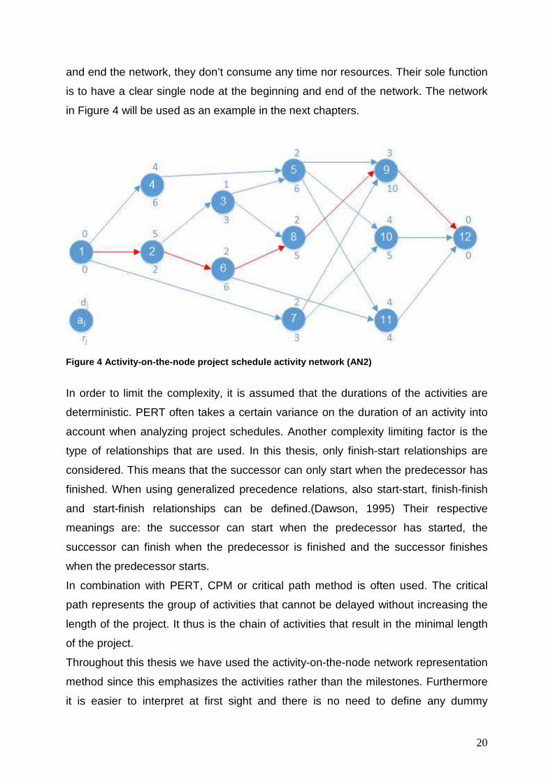
20

and end the network, they don’t consume any time nor resources. Their sole function

is to have a clear single node at the beginning and end of the network. The network

in Figure 4 will be used as an example in the next chapters.

In order to limit the complexity, it is assumed that the durations of the activities are

deterministic. PERT often takes a certain variance on the duration of an activity into

account when analyzing project schedules. Another complexity limiting factor is the

type of relationships that are used. In this thesis, only finish-start relationships are

considered. This means that the successor can only start when the predecessor has

finished. When using generalized precedence relations, also start-start, finish-finish

and start-finish relationships can be defined.(Dawson, 1995) Their respective

meanings are: the successor can start when the predecessor has started, the

successor can finish when the predecessor is finished and the successor finishes

when the predecessor starts.

In combination with PERT, CPM or critical path method is often used. The critical

path represents the group of activities that cannot be delayed without increasing the

length of the project. It thus is the chain of activities that result in the minimal length

of the project.

Throughout this thesis we have used the activity-on-the-node network representation

method since this emphasizes the activities rather than the milestones. Furthermore

it is easier to interpret at first sight and there is no need to define any dummy

Figure 4 Activity-on-the-node project schedule acti vity network (AN2)

21

activities besides the start and end activity. Other advantages identified by Turner

include the ease of drawing activity-on-the-node networks and the ability to write

network software more easily and the independency. (Turner, 1993)

Programming data representation

The network can be translated or decoded into static and dynamic data. The static

data includes the duration of the activities, the necessary resources for the execution

of each activity and the precedence relations of the activities. These will remain

identical throughout the scheduling process. The dynamic data are the starting times

of each activity, these will change throughout the process and are the eventual

outcome.

Both the aforementioned static and dynamic data will be saved into vectors. i.e. a

vector of durations, a vector of resource usages, a vector of successors and a vector

of starting times. For example figure 4, this results into a vector represented in table

1.

a1 a2 ... a12 d[aj] 0 5 1 4 2 2 2 2 3 4 4 0

Table 1 Example Duration Vector

For the decoding of the activity starting times, there are two options. The first one

consists of the absolute starting time of the activities and the second considers a

relative starting time. (Wall, 1996) The first method is straightforward and states an

exact starting time, independent of the starting time of other activities. Table 2 shows

an example of a vector with absolute starting times.

a1 a2 ... a12 st[aj] 1 4 6 8 9 14 10 18 8 17 19 19

Table 2 Absolute Starting Times

Activity one starts at day one, activity two starts at day four and activity three starts at

day six.

The second method does not state an absolute starting time but rather a relative

starting time of the activity i.e. the relative starting time indicates how many days

there are between the start of an activity and the end of the latest predecessor. The

vector of these relative starting times will be referred to as the float vector in the

remainder of the thesis.

22

Table 3 shows how a float vector is represented.

a1 a2 ... a12 fl[aj] 0 4 6 8 4 2 6 3 8 5 5 0

Table 3 Relative Starting Times

This float vector has to be interpreted in combination with the precedence relations to

result into the actual starting times of the activities. If you combine this with the

network of figure 4, the resulting starting times are calculated in table 4.

a1 a2 ... a12 st[aj] 0 4 15 8 20 11 6 19 30 27 27 33

Table 4 Resulting Starting Times

The start time of activity three is the end time of the latest predecessor (activity two)

which is nine. Add to this number the float value of six and you get the starting time

for activity three, i.e. fifteen.

We opted to go for the relative time representation for the simple reason that it is

impossible to break any precedence relations constraint since it is imbedded into the

definition of the float vector. If the absolute starting times are used, every schedule

that is produced needs to be tested if any precedence relation is violated and if

necessary repair these violations. An example of this is activity nine in table 2, which

starts at day eight while its predecessing activity seven starts at day 10. table 2 is

thus an example on an infeasible schedule.

Dataset

We execute the algorithm on three prototype activity network datasets. These activity

networks contain the same activities, i.e. twelve activities including a dummy start

and dummy end activity. Even the activity characteristics, concerning duration and

resource demand are identical. The only aspect that is different between the three

activity networks under research is the order in which the activities should be

executed. This order is visually represented by the arrows as the precedence

relations in the activity networks. Appendix A shows all three activity networks,

further denoted as activity network AN1, AN2 and AN3. Note that AN2 is discussed

previously in this section. These three networks are not chosen at random but have a

distinctive topological structure. We want to test how the algorithm reacts to activity

networks with a tendency to a very parallel structure compared to activity networks

23

with a tendency to a very serial structure. This is done by measuring the serial or

parallel indicator as a topological indicator to measure the network structure.

(Vanhoucke et al., 2008) This indicator has a value ranging from 0 to 1, with 0

meaning a complete parallel network structure and 1 meaning a complete serial

network structure. This indicator (I) is calculated using the formula below.

In this calculation, n indicates the number of activities excluding the dummy start and

end node and m denotes the maximum progressive level of the network.

(Elmaghraby, 1977) AN1, AN2 and AN3 have 0.11, 0.33 and 0.44 as respective

values for the serial parallel indicator (SP indicator). These values seem very low.

However when setting higher values, the tendency towards a serial structure is so

overwhelming that there is very limited scheduling flexibility. When the SP indicator is

0, which means that all activities are in a parallel structure, the scheduling flexibility is

maximal since there is not strict order in the activities. When the SP indicator is 1,

which means that all activities are in a serial structure, there is no scheduling

flexibility since the order of the activities is completely fixed.

We assume that parallel networks have a broader solution space and offer more

possibilities to the staffing of a project, possibly resulting in lower staffing costs.

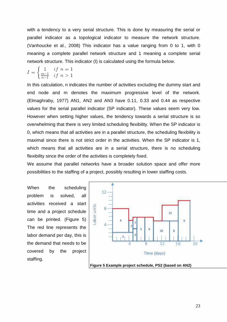
When the scheduling

problem is solved, all

activities received a start

time and a project schedule

can be printed. (Figure 5)

The red line represents the

labor demand per day, this is

the demand that needs to be

covered by the project

staffing.

Figure 5 Example project schedule, PS2 (based on AN 2)

24

4.2.2. Project Staffing representation

The project staffing representation revolves around the representation of the work

pattern. This work pattern is a binary vector indicating whether a day in the pattern is

a working day or a day off. An example of a work pattern and a combination of work

patterns to form the labor supply is shown below.

Pattern Workers 1 2 3 4 5 6 7 8 9 10 11 12 13 14 15 16 17 18 19 w1 1 0 0 1 1 1 1 1 1 0 0 1 1 1 1 1 1 0 1 1 w2 1 1 1 0 0 1 1 1 0 1 1 0 0 1 1 0 1 1 1 1 w3 2 1 1 1 1 0 1 1 0 1 1 1 1 0 1 1 1 1 1 1 w4 2 1 1 1 1 0 1 1 1 0 0 1 1 1 1 1 1 0 1 1 w5 3 1 1 1 1 1 0 0 1 1 1 0 0 1 1 1 1 0 1 1

Staffing (Supply) 8 8 8 8 5 6 6 6 6 6 5 5 7 9 8 9 3 9 9 Scheduling (Demand) 8 8 8 8 5 6 6 6 6 6 5 5 9 9 9 9 10 10 10 Ext / Idle (Difference) 0 0 0 0 0 0 0 0 0 0 0 0 2 0 1 0 7 1 1

Table 5 Work patterns forming labor supply Table 5 shows an example of staffing executed on AN2 and PS2. Five work patterns

are distinguished to carry out the labor defined by PS2. Nine workers are hired for

the project, work pattern one and two are executed by one worker each, work pattern

three and four are executed by two workers each and 3 workers have working

pattern five. The center of the table indicates whether a work pattern is on or off work

on a certain day. Work patterns three and four have an overtime unit on day four;

their first week contains six days of work in stead of the regular five days. In the

bottom part of the table, the total labor supply per day is calculated as the sum of the

individual active work patterns. The row below you can find the labor demand per day

as defined by PS2. The lowest row indicates whether external labor units (positive

value) should be hired or idle time (negative value) occurs for every day. Towards the

end of the project, external workers are hired. The difference of labor supply and

demand can also be shown in the project schedule graph. Below, you can find an

extended version of figure 5. The red line still shows the labor demand while the

green dotted line indicates the labor supply as defined by the staffing. Demand

exceeds supply towards the end of the project.

25

Figure 6 Labor supply and demand for AN2, PS2

26

4.3. Solution methods This section contains an overview of all

the methods that were taken into

consideration for the algorithm. The

structure of this section is guided by the

flowchart in figure 6. The flowchart

represents the different phases in the

algorithm. Each phase contains multiple

methods that contribute to the solution of

the problem. The topics will be

discussed in this order: Initialization,

Selection, Operation, Local Optimization,

Partial Evaluation, Reinsert, Ending

Condition an Evaluation. Figure 6

indicates the sections and subsections in

which the different methods are

discussed.

4.3.1. Initialization To start the algorithm, we need to initialize a population of schedules in the form of

float vectors. Although research has often neglected the importance of the

initialization phase, a bad initial population can lead to increased time-to-solution or

even getting trapped into local optima. A minimum of diversity in the population is

necessary to avoid premature convergence of the solutions towards suboptimal

regions of the solution space. To initialize our population, simple constructive

heuristics will be used.

To construct the schedule float vectors, we distinguish three groups of initialization

methods, i.e. random, uniform and Gaussian initialization.

Figure 7 Flowchart Genetic Algorithm, framework 2

27

I1 Random Initialization

In the random initialization method, a maximum float value (MFV) is determined.

Then a value is randomly generated in [0, MFV]. The parameterisation for MFV leads

to the following methods.

I1a MFV = 1 x AVG duration of activities

I1b MFV = 2 x AVG duration of activities

I1c MFV = 3 x AVG duration of activities

I2 Uniform Initialization

In the uniform initialization method, a central value (CV) and a deviation value (DV) is

determined. Then a value is uniformly generated in [CV-DV, CV+DV]. The biggest

difference with the random initialization method is that this method does not

necessarily include the value 0. If CV-DV would return a negative value, it is

automatically initiated with a 0. If a large amount of float values are generated using

this method, you will notice that they follow a uniform distribution. The parameters for

CV and DV led to the following methods.

I2a CV = 1 x AVG duration of activities DV= 0,5 x AVG duration of activities

I2b CV = 2 x AVG duration of activities DV = 0,5 x AVG duration of activities

I2c CV = 2 x AVG duration of activities DV = 1 x AVG duration of activities

Note that there is no method where CV = DV = AVG duration of activities since this

method is identical to method I1b.

I3 Gaussian Initialization

In the Gaussian method, a central value (CV) and a standard deviation value (SDV)

is determined. Then a value is generated conform the gaussian distribution with a

mean CV and a standard deviation SDV. This method differs from the two previous

ones by the fact that it allows more extreme values sine it has no maximum value,

i.e. there is no closed upper end.

If this method would return a negative value, it is automatically initiated with 0.

The parameters for CV and SDV led to the following methods.

I3a CV = 1 x AVG duration of activities SDV= 0,5 x AVG duration of activities

I3b CV = 1 x AVG duration of activities SDV= 1 x AVG duration of activities

I3c CV = 2 x AVG duration of activities SDV= 0,5 x AVG duration of activities

I3d CV = 2 x AVG duration of activities SDV= 1 x AVG duration of activities

28

I4 Combined Initialization

This method makes a combination of the previous methods I1, I2 and I3 to become

the initial population.

The pseudo code for the initialization phase can be found in figure 8.

Pick an Initialization method I1, I2, I3 or I4 (I)

Determine initialization characteristics MFV, CV, DV, SDV

While population not entirely filled

Create new empty float vector

While there are activities without float value

Select a random activity a

If activity a has no float value

Initialize activity a using initialization method I

Endif

Endwhile

Endwhile

Figure 8 Pseudo code Initialization methods

Other Initialization method

Another initialization method that was considered finds its background in RACP. It is

based of the maximum / minimum bounding strategy for determining the cheapest

resource availability levels for a project. (Demeulemeester, 1995)

The general idea is to calculate a resource availability constraint and use this

constraint in combination with a scheduling rule to generate initial schedules.

In a first step, calculate the minimum possible resource usage that would be

necessary if there would be a constant availability of resources over the span of the

project. This in fact, is equal to the resource usage of the most needy activity in the

project. Applying this to our example in figure 4, the minimum possible resource

usage is 10. This corresponds to the resource usage of activity 9. Secondly,

calculate the maximum possible resource usage that would be necessary if there

would be a constant availability of resources over the span of the project. For our

example, this resource usage is 19 and is the maximum resource usage that is

possible if activities 9, 10 and 11 would occur simultaneously. In a third step, the

29

activities will be scheduled using a basic priority rule and schedule generation

scheme. Step 3 is repeated with different priority rules and a resource constraint

ranging from 10 to 19. Each time step 3 is executed, this results in a schedule that is

put in the initial population.

4.3.2. Selection Once an initial population of schedules is available, we need to find a way to select

one or more schedules on which a certain operation will be performed later on.

These selected schedules are called parents. The key idea of this selection phase is

to select good parents, in order to give them an opportunity to pass on their good

genes onto the next generation. Likewise, this phase should also prevent the worst

solutions from passing on their inferior genes onto the next generation. (Sivaraj,

2011)

A distinction can be made between two types of selection methods or schemes, a

proportionate scheme and an ordinal-based scheme. (Sastry and Goldberg, 2001)

Using an ordinal-based scheme, the chance of an individual to be selected depends

on the ranking of the individual in the population based on a fitness measure.

With a proportionate scheme, the chance of an individual to be selected depends on

the relative fitness of the individual in comparison with the other individuals in the

population. In other words, with an ordinal-based scheme, the chance of being

selected merely depends on the fitness rank of the individual in the population, while

a proportionate scheme also takes into account how much one solution is better than

the other to determine the selection likelihood. The latter not only implies an order of

the individuals in the population but also a scaling measure to determine the relative

superiority of one individual to another.

In this section, we will take a closer look at three selection methods, a random

selection method, a roulette wheel selection method (proportionate scheme) and a

tournament selection (ordinal-based scheme).

30

S1 Random Selection

This selection method does not embed any intelligence. It merely selects 2

individuals randomly. This method does not give preference to individuals that are

more fit than others and therefore this method is perceived to be inferior compared to

other selection methods that make use of more intelligent criteria.

S2 Roulette Wheel Selection

As stated in the introduction, the roulette wheel selection method is a proportional

scheme to select individuals out of a population. The first step is to calculate a fitness

value for each of the individuals in the population. Depending on the algorithm being

used, this fitness value could be either the total cost (figure 2) or the average

squared deviation (figure 3). The second step assigns a probability to each individual

based on the fitness value. These probabilities are set out on a roulette wheel, the

bigger the probability of the individual to be taken, the bigger the circumference of

that individual on the roulette wheel will be. In the third step, the wheel gets spun and

wherever the wheel stops, this individual will be taken. To select another individual,

repeat the procedure starting from step two.

A small example will illustrate this method.

Assume five individuals and their respective fitness values. An increasing value

indicates a better individual. The circumference of the roulette wheel gets divided into

five parts, each part belonging to the selection of one individual. An example of the

division of the wheel is given in figure 9. The wheel gets spun and the individual is

chosen where the roulette wheel comes to a standstill.

31

Figure 9 Example Roulette Wheel

The pseudo code for the roulette wheel selection can be found in figure 10.

Calculate the fitness value of each individual

While necessary to select additional individual

Determine selection probability for each individual based on fitness value

Generate a random number, mimicking the spinning of a roulette wheel

Translate the outcoming number into the underlying individual

Endwhile

Figure 10 Pseudo code Roulette Wheel Selection

S3 Tournament Selection

The tournament selection method is an ordinal-based scheme to select individuals

out of a population. The first step consists of determining the rank-order of the

individual based on a fitness value. This value will again be the total cost or the

average squared deviation. This ranking will determine which individual wins in a

tournament. In the second step, two individuals are selected randomly. Thirdly, the

individual with the highest ranking wins the tournament and survives the selection

stage. Repeat steps two and three until enough individuals are selected.

The pseudo code for the tournament selection can be found in figure 11.

32

Calculate the fitness value of each individual

Make a ranking of the individuals based on fitness value

While necessary to select additional individual

Select 2 individuals randomly

Determine the winner based on the ranking

Endwhile

Figure 11 Pseude code Tournament Selection This tournament selection method can be extended by either adding additional

tournament rounds, such that an individual has to win 2 or more rounds before it is

selected or by adding more individuals competing in each round.

A big advantage of this method over the roulette wheel is that there are no scaling

issues. Since the tournament selection merely uses a rank, there is no need to

translate the difference in fitness in a different selection probability. (Whitley, 1989)

S4 Combined Selection

Selection method S4 uses all three aforementioned methods to select individuals.

Which method is used for each selection is determined on a random basis.

4.3.3. Operation On the (pair of) parents, operators will be executed in order to generate different

solutions, called ‘children’. The solutions can change drastically or just slightly.

The two main types of operations are crossover and mutation. (Luke and Spector,

1998) Crossover relies on the hypothesis that highly fit individuals in the population

consist of fit building blocks that can be mixed in order to become even more fit

individuals. It will push the population to converge into one or more local optima. This

process of convergence is often called intensification or exploitation. Mutation on the

other hand serves the goal of maintaining genetic diversity in the population.

Mutation thus fulfils the task of exploring the solution space. The aspects of mutation

and crossover are antagonists but are both equally important. On the one hand, we

need to be sure to have covered the solution space as much as possible through

genetic diversity. But on the other hand, we also want to make sure that we find the

best solution in the researched solution space through convergence into the best

areas.

33

The occurrence of crossover and mutation are reflected by their crossover rate and

mutation rate respectively, indicating the chance this operation will be executed on a

selected pair of parents. Fixing these rates to a general optimal value is very difficult

since they are very problem specific and they even depend on the stage of the

genetic algorithm. Research has been done on the determination of these values for

mutation and crossover both as a static constant and as a dynamic value, changing

over the course of the execution of the algorithm. (Lin et al, 2003)

In this section the following crossover operators will be discussed, including 1-point

crossover, 2-point crossover, blend crossover, mean crossover, extrapolation

crossover, uniform crossover and mutation.

C1 1-Point Crossover

This crossover operator heavily relies on the building block hypothesis as it cuts the

parents into two halves or blocks in order to recombine these blocks into the children.

The point where the parents should be cut is determined randomly. (Spears and

Anand, 1991)

An example is presented, 2 parents as float vectors containing the float value for 12

activities. The cut-off point is after the fourth activity.

a1 a2 ... a12 Parent 1 0 4 6 8 4 2 6 3 8 5 5 0

a1 a2 ... a12 Parent 2 0 2 1 4 3 9 5 7 3 10 2 0

These parents swap their float values after the cur-off point to create 2 children.

a1 a2 ... a12 Child 1 0 4 6 8 3 9 5 7 3 10 2 0

a1 a2 ... a12 Child 2 0 2 1 4 4 2 6 3 8 5 5 0

Assuming that parent 1 has a very fit first part and parent 2 has a very fit second part,

child 1 has a high probability of outperforming both parents.

34

C2 2-Point Crossover

This crossover operator is identical to the previous one besides the fact that there is

not a single cut-off point but 2 cut-off points that will chop the parent into 3 blocks to

be recombined. An example with cut-off points after the third and seventh float value.

a1 a2 ... a12 Parent 1 0 4 6 8 4 2 6 3 8 5 5 0

a1 a2 ... a12 Parent 2 0 2 1 4 3 9 5 7 3 10 2 0

Resulting children are constructed by swapping the middle block.

a1 a2 ... a12 Child 1 0 4 6 4 3 9 5 3 8 5 5 0

a1 a2 ... a12 Child 2 0 2 1 8 4 2 6 7 3 10 2 0

C3 Blend Crossover

Using the blend crossover operator, you do not copy and recombine genetic material

but you blend the corresponding genetic material, based on the distance between

them. (Eshelman and Schaffer, 1992) (Takahashi and Kita, 2001) The blending will

result into two values which are the boundaries for the newly generated child value.

The steps to be undertaken will be illustrated with an example.

a1 a2 ... a12 Parent 1 0 4 6 8 4 2 6 3 8 5 5 0

a1 a2 ... a12 Parent 2 0 2 1 4 3 9 5 7 3 10 2 0

Since the first activity has an identical float value, we will take the second activity as

an example. Firstly the distance between the two parents is calculated as the

difference between the respective float values, i.e. distance d = |4-2|.

(1)

In the second step, 2 boundary values (X1 and X2) are determined taking the lowest

float value, highest float value and the distance into account.

(2)

35

This would result in the following for our example.

(3)

In the third step, a new value gets generated randomly in the interval [X1,X2].

In our example, the interval is [1,5]. Do this for all activities until a entire child is

produced. The pseudo code for the blend crossover operator can be found in figure

12.

For every activity

Calculate the distance d between the two parents

Calculate the lower boundary, using distance d

Calculate the upper boundary, using distance d

Randomly generate a new float value between the boundaries

Endfor

Figure 12 Pseudo code Blend CrossOver

C4 Mean Crossover

The mean crossover operator will calculate the mean value of the two parents for

each activity and take this mean value as the new float value for the child (Wall,

1996). In case a non-integer value gets generated, the value will be randomly

rounded up or down. An example is shown below.

a1 a2 ... a12 Parent 1 0 4 6 8 4 2 6 3 8 5 5 0

a1 a2 ... a12 Parent 2 0 2 1 4 3 9 5 7 3 10 2 0

Applying the mean crossover operator will result in this child.

a1 a2 ... a12 Child 0 3 3 6 4 5 5 5 6 8 3 0

36

C5 Uniform Crossover

The uniform crossover is a very straightforward operator. To construct the child, for

each activity it will randomly take the float value of either parent. Extra intelligence

could be added in the sense that there is no random selection of the float value for

each activity but the fittest parent gets a higher probability. (Magalhães-Mendes,

2013)

Applying uniform crossover can result in he child shown below.

a1 a2 ... a12 Parent 1 0 4 6 8 4 2 6 3 8 5 5 0

a1 a2 ... a12 Parent 2 0 2 1 4 3 9 5 7 3 10 2 0

a1 a2 ... a12 Child 0 2 6 8 3 2 6 7 3 10 5 0

C6 Combined Crossover

This crossover method combines the five aforementioned crossover operators. Every

cycle, a new crossover operator gets chosen randomly.

Mutation

Mutation will be executed on a single individual. It does not combine 2 solutions but

merely alters an individual in a certain spot.

Mutation of an activity float value can be done neglecting the current value, meaning

that a reinitialization occurs. Another option is to take the current value into account

and mutate that value by adding or subtracting some value. Our mutation operator

neglects the current value.

This operator can be useful after a high number of generations, since at that point

solutions can converge. As mentioned in the introduction, mutation will maintain

some diversity that hinders the converging behavior of the population.

As the algorithm proceeds, it can be interesting to let the mutation rate evolve as

well. Modifying this rate inversely (proportional) to the population diversity could

prevent convergence. (Bäck, 1993)

37

4.3.4. Local Optimization

A regular genetic algorithm would, after a crossover operation, perform an evaluation

of the newly created child and consider whether to reinsert or to discard the child

from the population. However, we opted to insert local optimization or local search

first. Local search can optimize the children by looking into the nearby

neighbourhood in order to discover better solutions.

Local search has an intensification function as opposed to the diversification function.

Intensification means that you will further look into an area of the search space in

which you have found a solution yet, but want to optimize it further. Diversification

has the goal to look into unexplored search space in order to discover new valuable

solutions. (cfr. Mutation)

By applying local search iteratively on one solution, and by updating this solution by

its best neighbour, also known as hill climbing (Pisinger and Robke, 2010), you will

end up in a local optimum.

The local search operator can be a very simple swap operation or a small heuristic

that reschedules a part of the schedule.

This is very abstract but can be explained using a very simplified example in figure

13. This figure represents a two-dimensional landscape where the x-value represents

a location and f(x) represents the height of a certain location. The objective is to find

the location of the valley, i.e. the location with the lowest height. You could check

every location x going from 0 to infinite, calculate its corresponding height and then

conclude that the lowest point is location b. Another method would be to take random

location samples. These random locations are indicated by five arrows. Starting from

these five locations, you can explore the neighborhood for better locations. Starting

from location at arrow number two, you can search in two directions, right and left.

These two directions are called neighborhoods. When going to the right side you will

soon notice that the height is going up, so we will not explore that side.(hill climbing)

However when we go to the left, we notice the height to go down. Repeat this move

until you cannot go any lower. You will end up in point a. When following the same

neighborhood search strategy starting from arrow 3, you will end up in location b etc.

The great advantage of the second method, using local search, is that you need to

do less effort in order to find the valley. The disadvantage, however, is that you are

not sure whether you end up in the global optimum b or in a local optimum such as

38

location a and location c. But when the initial locations are strategically set out well,

the solution found should be close to the optimal solution.

Figure 13 Local search simplified

This example can relate to our problem in the sense that every x represents a

schedule or its float vector and f(x) represents the cost accompanying this schedule.

We want to find the lowest cost, so what we will do in the local search stage is to

alter a schedule a little bit in order to find better schedules. The project scheduling

problem, however, is a lot more complex because the neighborhood is extremely

large. Therefore good neighborhoods have to be defined in order to explore them

efficiently. Three local search strategies will be discussed into further detail, including

a simplified version of the Burgess and Killebrew heuristic, double-justification and 2-

exchange neighborhood.

L1 Burgess and Killebrew simplified RLP

This first local search method finds its origin in the heuristic proposed by Burgess

and Killebrew in 1962. The main reason for adopting this method is the observation

that, when keeping the length of the project constant, a more levelled solution will

return a lower cost. (observation in 6.1.) Since local search will hardly change the

length of the project, this gives the opportunity to translate the original problem into a

resource levelling problem.

We simplified the heuristic of Burgess and Killebrew in the sense that we do not use

any priority rule but merely drag activities back and forth in a random order. The

39

number of activities that will be considered for this dragging is determined by the

neighborhood depth variable. Furthermore we will not make use of the total sum of

squares but the average squared deviation (AVGSQDEV) as an indicator for

tendency towards a levelled solution. The following steps are executed in this

proposed method. Starting from a schedule, take a random activity and calculate its

earliest start time and latest start time. In terms of float values, the values represent 0

and the free float values respectively. Free float is defined as the maximum amount

of delay you can add to an activity without disturbing any subsequent activity. The

second step consists of an iterative procedure in which you schedule the activity at

each point in time between the earliest start and the latest start. At the end of each

iteration, a new schedule is constructed which gets evaluated in the third step using

the partial evaluation method, described in section 4.3.5. The essence of that

section states that the evaluation is not done based upon the fitness i.e. total cost of

the schedule but rather on the tendency towards a levelled solution. Based on this

partial evaluation, the best schedule is retained for further local optimization. These

three steps are repeated for a predetermined number of times that is comprised in

the neighborhood depth variable. The pseudo code for L1 can be found in figure 14.

For 1 to neighborhood depth

Select a random activity

Calculate the free float value or slack

For f: 0 to free float

Schedule the chosen activity using float value f

Calculate the AVGSQDEV for the resulting schedule

If Newly created schedule performs better

Retain this schedule for further local optimization

EndIf

EndFor

EndFor

Figure 14 Pseudo code LS1 Burgess and Killebrew simplified RLP

40

L2 Double-Justification

This method of double-justification comes from the area of the RCPSP in which the

project makespan minimization is the objective. (Muller, 2009) Double-justification

means that a schedule gets sequentially right-justified and left-justified. A right-

justified schedule is a schedule in which all activities are pulled as close as possible

to the end of the project while a left-justified schedule is one In which all activities are

scheduled as close as possible to the beginning of the project. A small adjustment

that we made to this procedure is the addition of a resource constraint during the

backward and forward scheduling that result into the right- and left-justified schedule

respectively. The following steps explain the procedure into further detail.

Start with calculating the maximum workload, this workload will be used later on as a

resource constraint. The second step consists of backwards scheduling, resulting in

a right-justified schedule. The order in which the activities are scheduled is

determined by their finishing time; the latest finishing activity gets scheduled first, as

late as possible and taking the resource constraint into account. The third step

consists of the forward scheduling resulting in a left-justified schedule. The order in

which the activities are scheduled is determined by their starting time; the earliest

starting activity gets scheduled first, as soon as possible and taking the resource

constraint into account. The pseudo code for this local optimization method can be

found in figure 15.

Calculate the maximum resource usage MAX, for resource constraint purposes

Determine order of activities for backward scheduling (~finishing times)

For every activity in order

Schedule activity as late as possible taking MAX into account

EndFor

Determine order of activities for forward scheduling (~starting times)

For every activity in order

Schedule activity as soon as possible taking MAX into account

EndFor

Figure 15 Pseude code Double-Justification

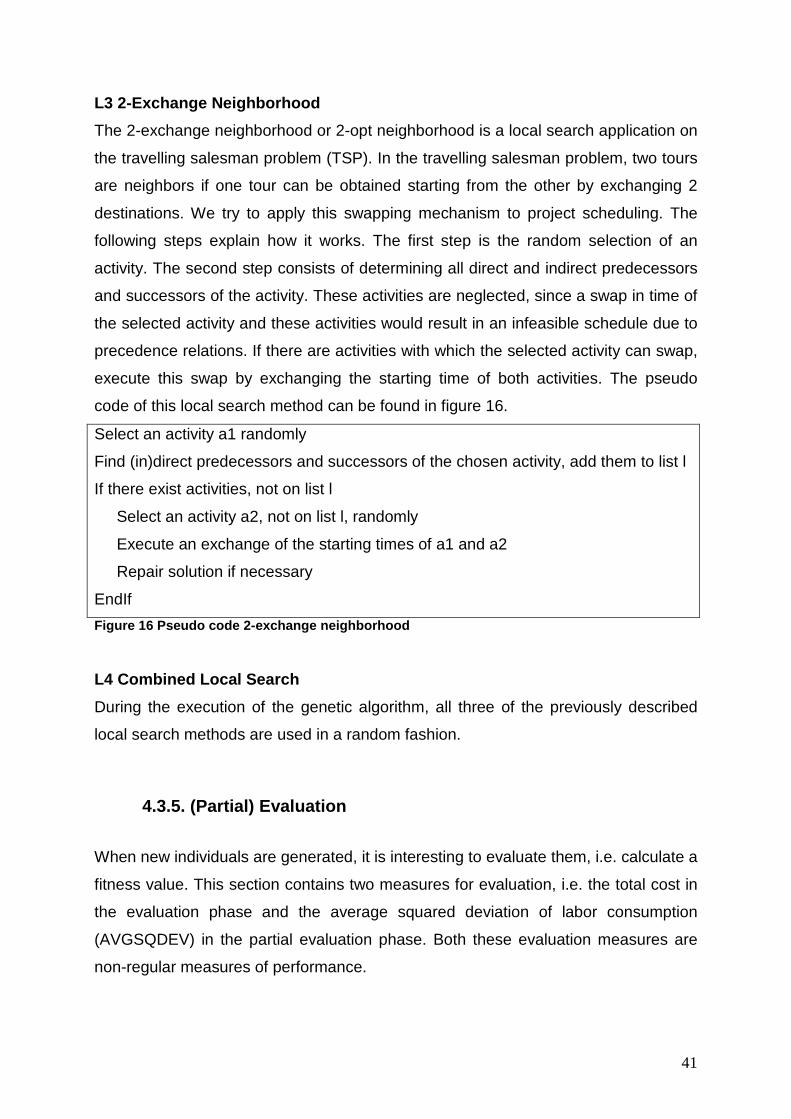
41

L3 2-Exchange Neighborhood

The 2-exchange neighborhood or 2-opt neighborhood is a local search application on

the travelling salesman problem (TSP). In the travelling salesman problem, two tours

are neighbors if one tour can be obtained starting from the other by exchanging 2

destinations. We try to apply this swapping mechanism to project scheduling. The

following steps explain how it works. The first step is the random selection of an

activity. The second step consists of determining all direct and indirect predecessors

and successors of the activity. These activities are neglected, since a swap in time of

the selected activity and these activities would result in an infeasible schedule due to

precedence relations. If there are activities with which the selected activity can swap,

execute this swap by exchanging the starting time of both activities. The pseudo

code of this local search method can be found in figure 16.

Select an activity a1 randomly

Find (in)direct predecessors and successors of the chosen activity, add them to list l

If there exist activities, not on list l

Select an activity a2, not on list l, randomly

Execute an exchange of the starting times of a1 and a2

Repair solution if necessary

EndIf

Figure 16 Pseudo code 2-exchange neighborhood L4 Combined Local Search

During the execution of the genetic algorithm, all three of the previously described

local search methods are used in a random fashion.

4.3.5. (Partial) Evaluation

When new individuals are generated, it is interesting to evaluate them, i.e. calculate a

fitness value. This section contains two measures for evaluation, i.e. the total cost in

the evaluation phase and the average squared deviation of labor consumption

(AVGSQDEV) in the partial evaluation phase. Both these evaluation measures are

non-regular measures of performance.

42

4.3.5.1. Total Cost (Evaluation)

To check the total cost of a schedule, we will let the staffing algorithm process the

generated schedule. The input is thus a project schedule and the outcome is a set of

workers with a certain work pattern. Based on this outcome, the total staffing cost of

the project can be calculated. The staffing is formulated and solved as a linear

programming problem. The solution of this problem is deterministic and optimal

meaning that given a certain input, always the same output is generated

(deterministic) and this output is the best possible (optimal). This linear problem was

provided by Prof. Dr. Maenhout and encoded into C++ which calls the Gurobi

Optimizer, a mathematical programming solver for different problems such as linear

programming and mixed integer programming problems.

This total cost calculation is the most important measure for fitness of a schedule, it

embodies the objective function as defined in section 2.3. However this calculation

takes a lot of computational effort, ranging from two to six seconds, depending on the

project length. Therefore, a second genetic algorithm framework is designed to

eliminate the calculation of the total cost as much as possible while affecting the

quality of the final schedule as little as possible.

4.3.5.2. Average Squared Deviation (Partial Evaluation) When doing a partial evaluation, the staffing algorithm will not be executed. This

performance measure is designed as an alternative for the total cost measure. It

represents a resource levelling approach. Observations in section 6.1 confirm that

the use of this measure is adequate for comparing schedules with an identical project

length. In that case, a lower AVGSQDEV will on average result in a lower total cost.

This assumption can be applied to the local optimization stage. At the end of each

search cycle, a performance measure needs to be calculated to determine the best

schedule in the neighborhood. Since these neighborhood search methods hardly

change the length of the project, the link between AVGSQDEV and total cost is

justified. This previously mentioned use of partial evaluation is present in both

genetic algorithm frameworks.

In order to further decrease computational efforts, the second framework goes one

step beyond. The second framework also uses the AVGSQDEV measure to decide

43

upon the reinsert of a schedule into the population. This often requires a comparison

of schedules with very different project lengths. Observations in section 6.1 do not

justify the use of the AVGSQDEV in this case, however it does not necessarily prove

that it should not be used. The big advantage of this method is the small

computational effort required for this calculation. The biggest disadvantage of this

method is that it is an approximation of the total cost measure, which means that a

lower AVGSQDEV will not necessarily always result in a lower total cost. This could

lead to situations where a schedule with a better AVGSQDEV but worse total cost

will replace a schedule with worse AVGSQDEV but better total cost during the

reinsert stage.

The formula to calculate the AVGSQDEV is given in figure 17.

Figure 17 Average squared deviation of resource con sumption T set of days in the scheduling horizn (index t)

A set of activities in the project (index j)

rj number of resources necessary to execute activity j

PL project schedule length

average resource use

This AVGSQDEV gives an impression of how levelled the resource demand of a

project schedule is. A low AVGSQDEV means that the resource consumption

throughout the project schedule is relatively equal and thus tends to be levelled. A

high average squared deviation points out that there will be big differences in

resource consumption between the different days in the schedule. Alternative

formulations of the levelling measure are the sum of squared deviations, the

weighted jumps in resource usage and the sum of absolute deviations. (Herroelen et

al., 1997)

44

4.3.6. Reinsert When new members (children) are generated, they should have the possibility to

enter the population. This section will handle this entering of the population. In the

first part, reinsert conditions are discussed. These conditions will decide whether a

newly created child is eligible to enter the population. The second part will handle the

population management. Population management will dictate how the population will

evolve throughout the generations.

4.3.6.1. Reinsert Conditions The algorithm can decide to let a child, that is generated out of existing parent

individuals, enter the population or not. Different conditions can be distinguished.

Some are relatively loose and will be passed very easily, making the population

improve slowly; other conditions are rather strict and as a consequence the

population fitness will improve either very fast or not at all. The insert condition

always results in the comparison of two or more schedules based on a performance

measure. For framework1, this performance measure is the total cost while for

framework2, this performance measure is the AVGSQDEV. The reinsert conditions

are described, assuming a steady-state population. This results in the replacement of

an existing member schedule by a new schedule. However as 4.3.6.2. points out,

also generational populations will be tested. In that case, there is no replacement of

an existing member but merely the addition of a new member into a new population.

R1 Outperform weakest schedule

This reinsert condition firstly calculates the performance measure of the newly

generated schedule and compares this to the performance measure of the weakest

schedule in the population. If the new schedule outperforms the weakest schedule,

this weakest schedule will be replaced by the new one.

45

R2 Outperform one parent

This reinsert condition firstly calculates the performance measure of the newly

generated schedule and compares this to the performance of both parents. If the new

schedule outperforms at least one parent schedule, the weakest parent will be

replaced by the new schedule.

R3 Outperform both parents

This reinsert condition firstly calculates the performance measure of the newly

generated schedule and compares this to the performance of both parents. If the new

schedule outperforms both parent schedules, the weakest parent will be replaced by

the new schedule.

R4 Outperform 25% of existing population

This reinsert condition firstly calculates the performance measure of the newly

generated schedule and compares this to the performance measure of all member

schedules in the population. If the new schedule outperforms at least 25% of the

schedules in the existing population, the weakest schedule will be replaced by the

new one.

R5 Outperform 50% of existing population

This reinsert condition firstly calculates the performance measure of the newly

generated schedule and compares this to the performance measure of all member

schedules in the population. If the new schedule outperforms at least 50% of the

schedules in the existing population, the weakest schedule will be replaced by the

new one.

R6 Outperform 75% of existing population

This reinsert condition firstly calculates the performance measure of the newly

generated schedule and compares this to the performance measure of all member

schedules in the population. If the new schedule outperforms at least 75% of the

schedules in the existing population, the weakest schedule will be replaced by the

new one.

46

Doubles

On top of the aforementioned reinsert conditions, an extra condition can be added.

This is the so-called doubles condition. This condition prohibits a new individual to

enter the population if that individual already exists in the population. It thus promotes

diversity in the population and will prevent convergence into local optima.

4.3.6.2. Population management

Population management or reproduction strategies dictate how the population

evolves throughout the execution of the algorithm. Two alternative startegies, i.e.

steady-state resulting in an overlapping population and generational reproduction

(Syswerda, 1991) resulting in a non-overlapping population are considered and a

hybrid form. (Noever, Baskaran, 1992)

P1 Steady-state population

This population management mechanism states that only a few individuals get

replaced at a certain point in time, keeping the size of the population constant. Which

individuals get replaced is defined by the reinsert condition. This results in the fact

that populations will overlap or different generations will overlap. It means that a child

(new generation) can enter the population of parents (old generation), and can mate

with its parents’ generation.

P2 Generational population

On the opposite side of the steady-state population, there is the generational

population. This population management mechanism will not replace individuals

separately but replace an entire population at once. It means that no replacement or

intermediate deletion of schedules from the population occurs. When enough

children are produced that pass the reinsert condition, the existing population will be

replaced by this new population of children. However, in order not to lose high-

performance member schedules from the previous population, a form of elitism or

elitist model is applied. (De Jong, 1975) We applied a simple elitist policy, stating that

when replacing the old population by a new population, the top 20% best schedules

of the old population should be forced into the new population. Depending on the

47

used framework, the performance measure to determine the best schedules is the

total cost and the AVGSQDEV for framework1 and framework2 respectively.

P3 Hybrid populations

This population management mechanism integrates the two previous systems. In the

beginning the population will act as a steady state population. After a certain amount

of replacements (80% of the population size), the population will act as a

generational population and it will be replaced as a whole.

4.3.7. Ending condition The cyclical character of the genetic algorithm makes it a never ending process.

Even when a local optimum or good solution is found, it can still generate new

children. A clear ending condition has to be stated to end the cycle. This ending

condition is a limitation and will never improve the objective function but rather limit

the time spent.

Static Ending Condition

This is a predefined, fixed ending condition which is not influenced by the course of

the genetic algorithm. Examples of this kind of ending condition are summed below.

• The algorithm stops after X operations

• The algorithm stops after X time units

• The algorithm stops after X evaluations

Dynamic Ending Condition

A dynamic ending condition is a condition that is influenced by the course of the

genetic algorithm. Examples of this are listed below.

• The algorithm will stop if no improvement is found in X operations

• The algorithm will stop if no improvement is found in X time units

• The algorithm will stop if the population contains X duplicates (if duplicates are

allowed)

• The algorithm stops after the fittest value of the population is lower than X

48

Hybrid ending condition

Dynamic and static ending conditions can be used in harmony. The static ending

condition will carry out the upper limit of the execution of the algorithm, expressed in

number of operations or time units etc. The dynamic ending condition would play the

role of early showstopper in case the solution is either satisfying enough or there is

no hope for improvement left and thus interrupting the execution is appropriate.

49

5. The algorithm Based on the computational results in table 8 of 6.3.1., a definite form of algorithm is chosen. The framework of choice is framework 2. Although this framework performs slightly worse than framework 1, the execution time is significantly shorter and thus better. Combination of methods and parameters:

• Population size 20 • Number of operations 100 • I1b Random Initialization

o MFV = 2 x AVG duration of activities • S3 tournament selection • C5 Uniform crossover • No mutation • L1 Burgess and Killebrew simplified RLP

o neighborhood depth =5 • R1 reinsert weakest in population

o P1 Steady state population o No doubles allozed

• No ending condition

50

6. Computational experiments In this chapter, the computational experiments of the methods described in chapter

four will be presented. In order to obtain the results, the solution methods are coded

into C++. The coding of this program took a couple hundreds of hours. This program

is then run on an Intel i3 core processor 2,13 Ghz and 4 Gb RAM. Executing this

program took several hundreds of hours of computational time.

In section 6.1. we provide an observation when first executing test cycles and

exploring the data it produces. Section 6.2. presents the benchmark for our test, this

benchmark gives an indication of how good the results, generate by the algorithm,

are. The last section contains the actual test results.

6.1. Observation link AVGSQDEV – Total cost When executing first test cycles, we were looking for performance measures besides

the total cost. Other measures, such as average float, project length and average

squared deviation were monitored. Afterwards, we tried to find connections between

these measures. One connection, between AVGSQDEV and total cost, is significant

and very useful practically. We plotted all schedules on a dispersion graph with

AVGSQDEV on the x-axis and Total cost objective on the Y-axis, which is shown in

figure 18. No clear correlation can be observed.

Figure 18 AVGSQDEV - Total Cost dispersion for all project lengths

Average Squared deviation - Objective

170

190

210

230

250

270

0 50 100 150 200 250 300

Average Squared deviation

Obj

ectiv

e

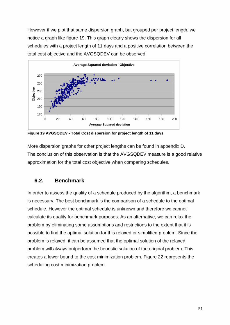
51

However if we plot that same dispersion graph, but grouped per project length, we

notice a graph like figure 19. This graph clearly shows the dispersion for all

schedules with a project length of 11 days and a positive correlation between the

total cost objective and the AVGSQDEV can be observed.

Figure 19 AVGSQDEV - Total Cost dispersion for proj ect length of 11 days

More dispersion graphs for other project lengths can be found in appendix D.

The conclusion of this observation is that the AVGSQDEV measure is a good relative

approximation for the total cost objective when comparing schedules.

6.2. Benchmark In order to assess the quality of a schedule produced by the algorithm, a benchmark

is necessary. The best benchmark is the comparison of a schedule to the optimal

schedule. However the optimal schedule is unknown and therefore we cannot

calculate its quality for benchmark purposes. As an alternative, we can relax the

problem by eliminating some assumptions and restrictions to the extent that it is

possible to find the optimal solution for this relaxed or simplified problem. Since the

problem is relaxed, it can be assumed that the optimal solution of the relaxed

problem will always outperform the heuristic solution of the original problem. This

creates a lower bound to the cost minimization problem. Figure 22 represents the

scheduling cost minimization problem.

Average Squared deviation - Objective

170

190

210

230

250

270

0 20 40 60 80 100 120 140 160 180 200

Average Squared deviation

Obj

ectiv

e

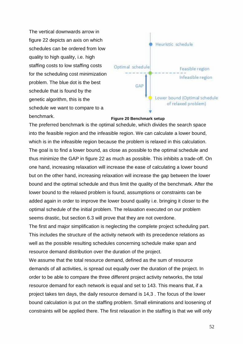
52

The vertical downwards arrow in

figure 22 depicts an axis on which

schedules can be ordered from low

quality to high quality, i.e. high

staffing costs to low staffing costs

for the scheduling cost minimization

problem. The blue dot is the best

schedule that is found by the

genetic algorithm, this is the

schedule we want to compare to a

benchmark.

The preferred benchmark is the optimal schedule, which divides the search space

into the feasible region and the infeasible region. We can calculate a lower bound,

which is in the infeasible region because the problem is relaxed in this calculation.

The goal is to find a lower bound, as close as possible to the optimal schedule and

thus minimize the GAP in figure 22 as much as possible. This inhibits a trade-off. On

one hand, increasing relaxation will increase the ease of calculating a lower bound

but on the other hand, increasing relaxation will increase the gap between the lower

bound and the optimal schedule and thus limit the quality of the benchmark. After the

lower bound to the relaxed problem is found, assumptions or constraints can be

added again in order to improve the lower bound quality i.e. bringing it closer to the

optimal schedule of the initial problem. The relaxation executed on our problem

seems drastic, but section 6.3 will prove that they are not overdone.

The first and major simplification is neglecting the complete project scheduling part.

This includes the structure of the activity network with its precedence relations as

well as the possible resulting schedules concerning schedule make span and

resource demand distribution over the duration of the project.

We assume that the total resource demand, defined as the sum of resource

demands of all activities, is spread out equally over the duration of the project. In

order to be able to compare the three different project activity networks, the total

resource demand for each network is equal and set to 143. This means that, if a

project takes ten days, the daily resource demand is 14,3 . The focus of the lower

bound calculation is put on the staffing problem. Small eliminations and loosening of

constraints will be applied there. The first relaxation in the staffing is that we will only

Figure 20 Benchmark setup

53

make use of regular time units which have a cost of 2, since these are the cheapest.

This means that we do not make use of overtime units and external time units,

incurring a respective cost of 3 and 4. Also the possible presence of idle time, which

costs 1, is neglected. The relaxation implicitly defines every worker to work five days

per week. He cannot work more, because that would imply an overtime unit and he

shouldn’t work less because idle time is neglected.

The second relaxation is that we allow ‘fractional employees’ to work. For example, if

there is a workload that would require 9,5 workers to execute, the real problem would

require to hire 10 workers to execute the load. The relaxed problem however accepts

this 9,5 fractional value.

Based on these relaxations, a lower bound for the cost of a schedule can easily be

calculated. This lower bound is dependent on the duration of the project and given in

figure 21.

Figure 21 Lower bound benchmark in function of proj ect duration

An example of the calculation is given for a project duration of 17 days. (lower bound

= 374)

Total resource demand 143 units (A)

Project duration 17 days (B)

Max available days per worker 13 days (C)

Amount of workers necessary (A/C) 11 workers (D)

Cost per worker per day of project 2 (E)

Total Cost (E*B*D) 374

Lower Bound

335

345

355

365

375

385

395

405

9 10 11 12 13 14 15 16 17 18 19 20 21 22 23 24 25 26

Project Duration

Tot

al C

ost

Lower Bound

54

The calculation of the max available days per worker is based on the fact that each

worker works five days per week, meaning that he will have 4 days off in the span of

17 days. If the project would have a duration of 18 or 19 days a worker would also

have 4 days off. However if the project would have a duration of 20 or 21 days, every

worker is required to take 5 and 6 days off respectively.

This evolution in ratio between days off and project duration explains why the lower

bound graph goes down during the first five days of the week and makes an upwards

spark during the last 2 days of the week. (figure 21) The evolution in that ratio also

explains the general upwards trend of the cost in function of the project duration.

The lower bound graph applies to all three project activity networks since the total

resource demand of each project activity network is identical and the remainder

differences are relaxed. The graph can be limited by cutting off an upper and lower

bound to the project duration. The upper bound is the fixed project deadline of 21

days, this is identical for every activity network. The lower bound represents the

critical path of the activity schedule and is different between activity networks. If, for

example the critical path is 14 days, it Is impossible to attain a cost of 343, which can

only be accomplished with a project duration of 12 days.

6.3. Results In the results section, three topics will be discussed. The first topic handles the basic

cycles. These are the cycles necessary to determine the best combination of

methods, described in section 4.3, for each different framework of the algorithm and

for each different activity network. There are 2 frameworks of the algorithm and 3

different activity networks. The second section on the stage contributions will consist

of an analysis that determines the importance of each stage in the genetic algorithm.

By removing or altering these stages and measuring the consequences on the total

cost, the importance is quantified. This will only be done for the best algorithm on

AN2. The third section consists of tuning different parameters in the algorithm; this

also includes a sensitivity analysis on some parameters, emphasizing their

importance or worthlessness. This will also only be done for the best algorithm on

AN2.

55

6.3.1. Basic cycles A basic cycle contains the process of finding the best algorithm for an activity

network in combination with an algorithm framework. Since we have two frameworks

and three activity networks, six basic cycles will be performed. A basic cycle consists

of several phases. In each phase, the algorithm framework is run multiple times,

each time the algorithm consists of different solution methods as defined by section

4.3. In the first phase or ‘Base case’, we allow all solution methods to be chosen. In

the last or ‘Best’ phase, only one solution method per stage remains. In the phases in

between, we gradually eliminate the eligible solution methods by removing the least

performing or by retaining the best performing methods. In phase ‘Best X’, we make

sure that only about ten different combinations of solution methods remain.

Elimination is based on the cost that is on average associated with the solution

method. A summary of the elimination process of each basic cycle is given in

appendix B, which states every eligible solution method at a certain phase in the

basic cycle in combination with the average cost of that phase.

A single exception to the elimination rule, which states that the least performant

solutions methods get eliminated, is made for local optimization method L2. This

method is often removed from the possibilities despite its seemingly high

performance. The algorithms that made use of L2 show no or very limited diversity in

its resulting best solution. This gives an indication that no real exploration of the

neighborhood occurs in spite of finding a good solution.

For each basic cycle, the minimum, maximum and average costs per phase are

indicated in a table and a graph. The tables and graphs for AN2 are shown below,

the tables and graphs for AN1 and AN3 are available in appendix C.

AN2 Framework 1

Phase Average Min Max Base Case 402,06 383 450 1st Exclusion 391,04 380 410 2nd Exclusion 388,91 378 401 Best X 386,74 373 405 Best 385,34 373 400

Table 6 Total Cost evolution basic cycle AN2 Framew ork1

56

Figure 22 Total Cost evolution basic cycle AN2 Fram ework1

AN2 Framework 2

Phase Average Min Max Base Case 403,51 383 458 1st Exclusion 389,67 373 416 2nd Exclusion 389,09 377 414 Best X 387,03 378 402 Best 386,29 378 403

Table 7 Total Cost evolution basic cycle AN2 Framew ork2

Figure 23 Total Cost evolution basic cycle AN2 Fram ework2

Total Cost evolution

370

380

390

400

410

420

430

440

450

460

Base Case 1stExclusion

2ndExclusion

Best X Best

Phase

Tot

al C

ost

Average

Min

Max

Total Cost evolution

370

380

390

400

410

420

430

440

450

460

Base Case 1stExclusion

2ndExclusion

Best X Best

Phase

Tot

al C

ost

Average

Min

Max

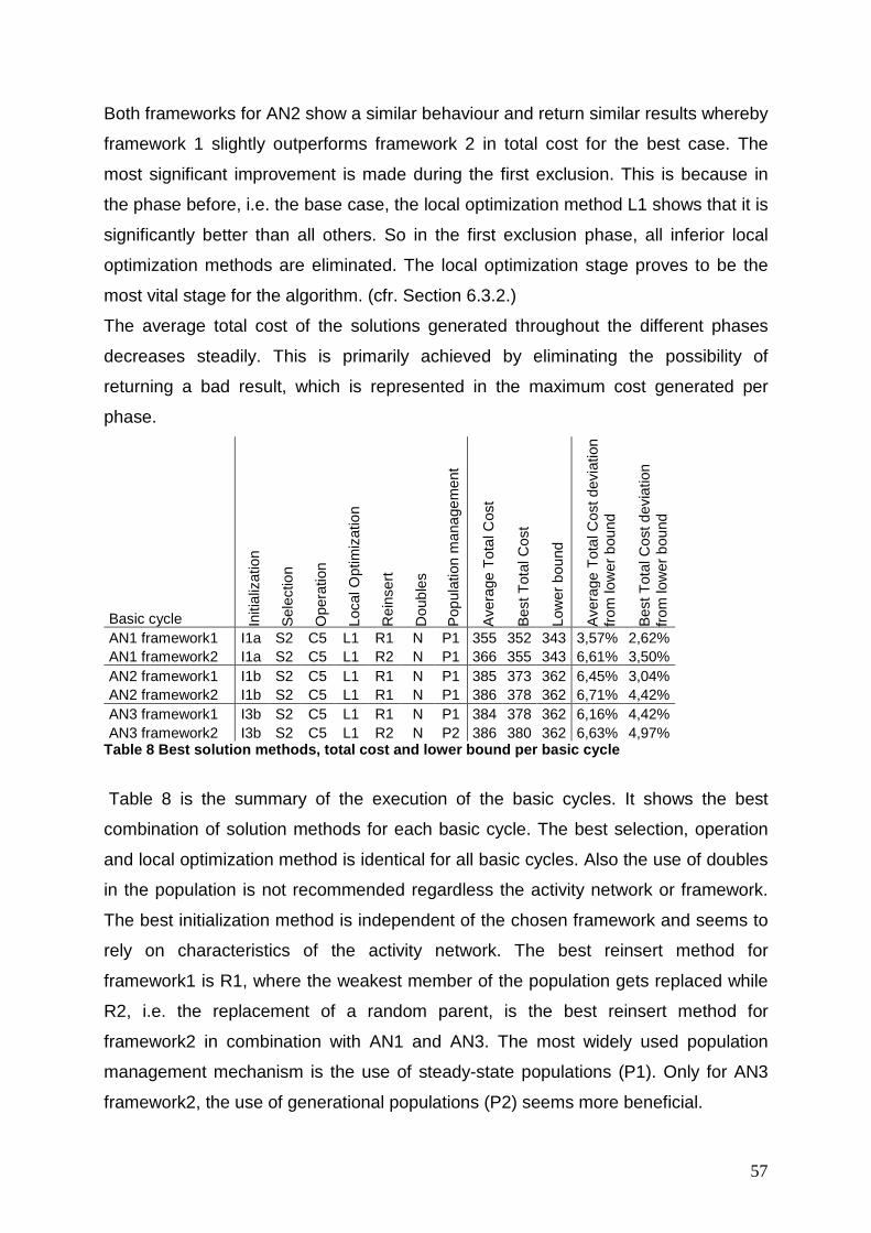
57

Both frameworks for AN2 show a similar behaviour and return similar results whereby

framework 1 slightly outperforms framework 2 in total cost for the best case. The

most significant improvement is made during the first exclusion. This is because in

the phase before, i.e. the base case, the local optimization method L1 shows that it is

significantly better than all others. So in the first exclusion phase, all inferior local

optimization methods are eliminated. The local optimization stage proves to be the

most vital stage for the algorithm. (cfr. Section 6.3.2.)

The average total cost of the solutions generated throughout the different phases

decreases steadily. This is primarily achieved by eliminating the possibility of

returning a bad result, which is represented in the maximum cost generated per

phase.

Basic cycle Initi

aliz

atio

n

Sel

ectio

n

Ope

ratio

n

Loca

l Opt

imiz

atio

n

Rei

nser

t

Dou

bles

Pop

ulat

ion

man

agem

ent

Ave

rage

Tot

al C

ost

Bes

t Tot

al C

ost

Low

er b

ound

Ave

rage

Tot

al C

ost d

evia

tion

from

low

er b

ound

Bes

t Tot

al C

ost d

evia

tion

fr

om lo

wer

bou

nd

AN1 framework1 I1a S2 C5 L1 R1 N P1 355 352 343 3,57% 2,62% AN1 framework2 I1a S2 C5 L1 R2 N P1 366 355 343 6,61% 3,50% AN2 framework1 I1b S2 C5 L1 R1 N P1 385 373 362 6,45% 3,04% AN2 framework2 I1b S2 C5 L1 R1 N P1 386 378 362 6,71% 4,42% AN3 framework1 I3b S2 C5 L1 R1 N P1 384 378 362 6,16% 4,42% AN3 framework2 I3b S2 C5 L1 R2 N P2 386 380 362 6,63% 4,97%

Table 8 Best solution methods, total cost and lower bound per basic cycle

Table 8 is the summary of the execution of the basic cycles. It shows the best

combination of solution methods for each basic cycle. The best selection, operation

and local optimization method is identical for all basic cycles. Also the use of doubles

in the population is not recommended regardless the activity network or framework.

The best initialization method is independent of the chosen framework and seems to

rely on characteristics of the activity network. The best reinsert method for

framework1 is R1, where the weakest member of the population gets replaced while

R2, i.e. the replacement of a random parent, is the best reinsert method for

framework2 in combination with AN1 and AN3. The most widely used population

management mechanism is the use of steady-state populations (P1). Only for AN3

framework2, the use of generational populations (P2) seems more beneficial.

58

The best solution method combinations for all basic cycles are very similar and also

yield similar results compared to the lower bound benchmark. The distance between

the average total cost, which is the total cost the basic cycle using the best methods

returns on average, and the lower bound benchmark is 6% - 7%. AN1 framework1 is

an exception with a distance of only 3,5%. Knowing that the lower bound returns a

better cost value than the optimal total cost, we know that the actual distance

between the average total cost and the optimal total cost is even smaller than the

6%-7% and 3,5%. If the best total cost, which is the best cost the basic cycle using

the best methods returns, is compared to the lower bound benchmark, a gap of 2%-

5% is noticed. The relative gaps between the total costs and the lower bound also

illustrate that framework1 consistently outperforms framework2 in terms of fitness.

6.3.2. Stage contributions In this section, we will further investigate to which extent each stage in the genetic

algorithm contributes to the total cost objective function. This contribution testing is

done by either removing a certain stage from the genetic algorithm or by replacing

the method by its worst alternative. This is only applied to AN2 framework2.

Initialization

Removing the initialization stage is simply impossible since an initial population

needs to be constructed with some logic. Therefore we compare the best initialization

method (I1b) to the worst tested initialization method. A deterioration of the total cost

from 386,29 to 392,86 or 1,7% is determined.

Selection

The best selection method is the tournament selection (S2). When replacing this

method by random selection, while keeping all other methods equal, only a small

deterioration from 386,29 to 386,92 or 0,16% is assessed.

Operation

The best method for this stage is the uniform crossover operator. When executing

the same algorithm but without this operator, the total cost goes up from 386,29 to

390,77 or 1,16%.

59

Local Optimization

The best local search method L1, which searches in the neighborhood for more

levelled schedules is the best local optimization method being tested. However, if we

remove this stage from the algorithm while keeping all other stages equal, the total

cost worsens drastically from 386,29 to 403,36 or 4,42%.

Reinsert condition

The best reinsert condition under consideration is the replacement of the weakest

member in the current population (R1). When removing this condition and thus

always reinsert a newly created child into the population, replacing an existing

member randomly, the total cost increases from 386,29 to 391,35 or 1,31%.

Population management

The best population management mechanism is the use of steady-state populations

(P1). However when applying the worst alternative method, i.e. generational

populations (P2), the total cost only worsens from 386,29 to 387,76 or 0,38%.

Conclusion

The local optimization stage has the most significant impact on the total cost, it

account for over 4% when removing this optimization and keeping all other stages

equal. The initialization, operation and reinsert condition have a moderate impact of

little over 1%. The selection stage and the population management have a very

minor impact on the total cost.

6.3.3. Sensitivity Analysis In this section, the computational results of a sensitivity analysis are shown. The start

case is the best algorithm associated with AN2 framework2. (also specified in

chapter 5) In the remainder of the section, we will refer to the configuration of the

algorithm as the ‘start case’. In this section we will focus on the influence of changing

some parameters on the outcome of the algorithm.

First of all, we will have a closer look at the population size and the number of cycles

or operations performed. Then we will check the influence of allowing doubles to

60

enter the population, the number of iterations or neighborhood depth in local

optimization, the use of mutation and an ending condition on the total cost of the

resulting schedule and the execution times necessary to obtain these schedules.

Population size and number of operations

The start case considers a population size of 20 schedules and the execution of 100

operations. We now expand these possibilities to 10, 20, 50 and 100 schedules as

population size and 50, 100, 250, 625, 1500 and 3000 as number of executed

operations. Besides these two dimensions, which will guide us, the total cost and

execution times are 2 other resulting dimensions that will be monitored.

Increasing the population size and the number of operations to be executed will

increase the execution time. However the relationship between the population size /

number of operations and the total cost is not that straightforward. An assumption

could be that more operations will result in better total cost. This is not necessarily

true because of the setup of framework2. As section 4.1.2. states ‘The disadvantage

(of framework2) however is that it is possible that the best schedule present in the

population gets replaced by another one during the execution of the algorithm.’ This

is exactly what happens after a very large amount of operations. The AVGSQDEV in

the population becomes extremely low and good solutions get replaced by worse.

This is illustrated by figure 24.

Figure 24 Total cost Vs number of operations for di fferent population sizes

Total cost Vs number of operations for different po pulation sizes

382

384

386

388

390

392

50 100 250 625 1500 3000

Operations

Tot

al C

ost 10 schedules

20 schedules

50 schedules

100schedules

61

For small population sizes of 10 or 20 schedules, the total cost seems to deteriorate

when operating a high number of operations. For population sizes of 50 and 100

schedules, this phenomenon is also assumed to happen, be it at much higher levels

of executed operations. In general we can assume the graphs to be U-shaped,

whereby the second leg of the U does not come that high. The optimal number of

operations, i.e. the bottom of the U-shape, increases with the size of the population.

Similarly, the influence of increasing population sizes on the total cost, when keeping

the number of operations constant can be depicted. This is done in figure 25.

Figure 25 Total cost Vs population size for differe nt number of operations

For algorithms with a large number of operations, the increased size of the

population is a positive influence on the total cost. This can be explained by the fact

that a larger population size will accommodate a larger extent of diversity and thus

better exploration of the solution space which increases the chance at finding better

solutions. However for algorithms with a relatively low number of operations, a large

population size had a negative influence on the total cost. This is graphically shown

in figure 25 where the pink and yellow graphs go upwards when applying large

population sizes. This can be explained by that fact that the number of operations is

so low, in comparison with the population size, that the algorithm has no chance to

nest itself into a (local) optimum.

Total cost Vs population size for different number of operations

376

378

380

382

384

386

388

390

392

394

10 20 50 100

Schedules

Tot

al C

ost

50 operations

100 operations

250 operations

625 operations

1500 operations

3000 operations

62

For academic purposes, the interaction between the population size / number of

operations and the total cost is interesting. However for practical purposes, the

relationship between the execution time and the total cost is much more interesting.

Therefore we combine the aforementioned two logic statements:

• The number of operations and the population size has an influence on the

execution time (logic statement 1)

• The number of operations and the population size has an influence on the

total cost (figure 24 and figure 25) (logic statement 2)

We translate these into a relationship between execution time and the total cost. This

logic and its four dimensions are embodied in figure 26 and represent a trade-off

between total cost and execution time.

Figure 26 Trade-Off Total Cost Vs. Execution Time

Every dot in figure 26 represents a combination of population size and number of

executed operations. For example, the blue graph represents the dots with a

population size of 10 schedules. The first dot in the blue graph stands for 50

operations, the second for 100 operations, the third for 250 operations and so on.

Every dot also has an according execution time (logic statement 1) and a total cost

(logic statement 2) which are both dependent on the population size and number of

operations. This results in a total cost versus execution time trade-off. The trade-off

should be read as follows: When keeping the population size constant, an increasing

execution time will on average improve the total cost and vice versa. Note the

upwards trend in the graph for population sizes of 10 and 20 schedules, this has the

same reasoning as the one explained by figure 24.

Trade-off total cost Vs. execution time

382

384

386

388

390

392

0 200 400 600 800 1000 1200

Execution time (seconds)

Tot

al C

ost 10 schedules

20 schedules

50 schedules

100schedules

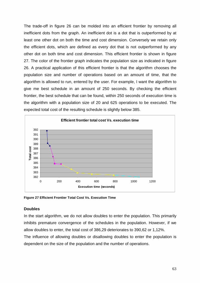
63

The trade-off in figure 26 can be molded into an efficient frontier by removing all

inefficient dots from the graph. An inefficient dot is a dot that is outperformed by at

least one other dot on both the time and cost dimension. Conversely we retain only

the efficient dots, which are defined as every dot that is not outperformed by any

other dot on both time and cost dimension. This efficient frontier is shown in figure

27. The color of the frontier graph indicates the population size as indicated in figure

26. A practical application of this efficient frontier is that the algorithm chooses the

population size and number of operations based on an amount of time, that the

algorithm is allowed to run, entered by the user. For example, I want the algorithm to

give me best schedule in an amount of 250 seconds. By checking the efficient

frontier, the best schedule that can be found, within 250 seconds of execution time is

the algorithm with a population size of 20 and 625 operations to be executed. The

expected total cost of the resulting schedule is slightly below 385.

Figure 27 Efficient Frontier Total Cost Vs. Executi on Time

Doubles

In the start algorithm, we do not allow doubles to enter the population. This primarily

inhibits premature convergence of the schedules in the population. However, if we

allow doubles to enter, the total cost of 386,29 deteriorates to 390,62 or 1,12%.

The influence of allowing doubles or disallowing doubles to enter the population is

dependent on the size of the population and the number of operations.

Efficient frontier total cost Vs. execution time

382

383

384

385

386

387

388

389

390

391

392

0 200 400 600 800 1000 1200

Execution time (seconds)

Tot

al c

ost

64

Allowing doubles has as a direct implication that the population can converge faster

towards a (local) optimum. Nevertheless this optimum seems to be of lower quality in

most cases. This is because the converging of the population prevents the program

from exploring the broader solution space in order to find better solutions.

In table 9 we calculated the difference in total cost between the start algorithm with

doubles and the start algorithm without doubles, for each combination of population

size and number of operations. An example of how the table should be read: When

using the start algorithm with population size 10 and 50 operations, the total cost of

the algorithm that uses doubles is 5,24 higher than the algorithm version without

doubles. Overall, the algorithm without doubles is the best however we indicated a

region in yellow where the algorithm with doubles outperforms or returns similar

results to the algorithm without doubles. This area has relatively big population sizes

and a relatively small number of operations. The reason why the algorithm with

doubles is able to perform well in this area is because it forces the population to

converge faster into (local) optima while the algorithm without doubles will converge

slower towards possible (local) optima.

Population size 10 20 50 100 Operations 50 5,24 -1,17 0,22 -0,69 100 5,17 4,33 0,2 0,46 250 10,76 8,54 2,13 -0,2 625 9,44 10,57 7,61 6,06 1500 8,75 11,13 11,69 12,86 3000 8,25 9,74 12,05 14,51

Table 9Total cost comparison with and without doubl es in the population

When plotting this algorithm as an efficient frontier, we assess that this new efficient

frontier is entirely outperformed by the efficient frontier of the algorithm without

doubles. We can conclude that none of the combinations of population size and

number of operations in the yellow area of table 9 is on the efficient frontier of the

algorithm with doubles.

The newly added efficient frontier in figure 29 is plotted above the previously

determined efficient frontier.

65

Figure 28 Efficient Frontier Total Cost Vs. Executi on Time, with / without doubles

Local search iterations

For local optimization method L1, an extra parameter can be tuned. This parameter

defines the number of local search iterations or the neighborhood depth of the

method. As defined in section 4.3.4. this parameter determines how many times we

consecutively check the neighborhood starting from a different activity. Logically, the

more iterations, the better the outcome will be.

Figure 29 Total Cost Vs. Number of Iterations Figure 29 shows a decreasing improvement of the total cost. While the improvements

are significant between one and five iterations, the improvement at five or more

iterations stagnates.

Efficient frontier Cost Vs. Execution time

382

384386

388

390

392394

396

0 200 400 600 800 1000 1200

Execution time

Cos

t

Cost Vs. neighborhood depth

385

386

387

388

389

390

391

392

393

394

1 3 5 7 9

Neighborhood depth

Tot

al C

ost

Total cost

66

Mutation

Figure 30 Total Cost Vs. Mutation Percentage Figure 30 shows the evolution of the total cost when increasing the mutation

probability. This graph does not provide us enough information to make a clear

statement on the use of mutation. Nevertheless we can state that a high mutation

percentage will probably not enhance the working of the algorithm. The reason could

be that the operation and local search process probably already contain enough

exploration possibilities. The start algorithm does not make use of mutation. As

stated in chapter 5, the local search method is very dominant and has a very

intensifying function. This could push the cross-over operator into the direction of an

exploring function, in order to become better solutions. The used cross-over operator

c5 is uniform cross-over, which is especially in the beginning of the algorithm

execution very exploratory. Since the cross-over method bears the exploratory

function, mutation is no longer necessary. We must note that this is a wild guess.

Ending condition

An ending condition will end the execution of the algorithm before it reaches the

predefined number of operations and will thus shorten the execution time of the

algorithm. However the goal is to shorten the execution time without affecting the

objective function too much. Before fine-tuning this parameter, we created an

indicator stating the moment when the best solution is found. This indicator is

represented as a percentage, the best schedule percentage or BSP. A value of 40%

means that the best schedule of the algorithm was found after 40 percent of the

Total cost Vs Mutation rate

386

386,2

386,4

386,6

386,8

387

387,2

387,4

387,6

387,8

0 2 5 10 25

Mutation rate (in %)

Tot

al C

ost

Total cost

67

execution time and that 60 percent of the execution time is wasted. The BSP

however does not give any indication on the quality of the solution.

Figure 31 BSP Vs number of operations

Figure 31 shows the influence of the number of operations on the BSP. An increase

of the number of operations logically decreases the BSP.

Overall, the size of the population increases the BSP. Also this is very logic since it

takes more operations in a big population to become good solutions than in smaller

populations.

In this section, we will zoom in on the algorithm setup with a population of 20

schedules and 100 operations. This algorithm has a BSP of 57% and an expected

total cost of 386,29. Since the objective function calculation, in framework2 of the

algorithm, happens completely at the end of the algorithm, the BSP is only known

afterwards when the whole algorithm is run. Therefore we cannot calculate whether

improvement is made or not during execution. We will again rely on the AVGSQDEV

as a relevant approximation for the total cost objective. When no improvement in this

indicator is assessed, the execution can stop.

We ran the algorithm on an ending condition of 5, 10, 20 and 30. This means that, if

no improvement in AVGSQDEV is respectively found after 5, 10, 20 or 30 operations,

no more operations will be executed and the termination of the algorithm will start by

evaluating the schedules present in the population.

Figure 32 shows the influence of the ending condition on the total cost of the

schedule. A strict ending condition can lead to drastic deterioration of the cost of the

schedule.

Best solution Vs. Number of operations

0

0,1

0,2

0,3

0,4

0,5

0,6

0,7

50 100 250 625 1500 3000

Operations

Bes

t Sol

utio

n P

erce

ntag

e

10 schedules

20schedules

50 schedules

100 schedules

68

Figure 32 Total cost Vs ending condition Figure 33 shows the influence of the ending condition on performed operations. The

maximum possible number of operations is 100. Using a very strict ending condition

of 5, we observe that only 11 operations are executed. Using an ending condition of

30, this amount increases to 65 which is still significantly below 100.

Figure 33 Performed operations Vs ending condition

We come to the conclusion that, for a strict ending condition, the gain in number of

performed operations can be significant. Figure 33 shows the number of performed

operations going down from 100 to 11, which is a decrease of 89%.

Total cost Vs ending condition

388

390

392

394

396

398

400

402

5 10 20 30

Ending condition

Tot

al C

ost

Total Cost

Performed operations Vs ending condition

10

20

30

40

50

60

70

5 10 20 30

Ending condition

Per

form

ed O

pera

tions

Performed Operations

69

7. Conclusions and further research The first important conclusion is that a basic genetic algorithm with limited complexity

is able to handle and manage the integrated project scheduling and project staffing

problem. With a total cost expectation of maximum maximorum 7% higher than the

lower bound benchmark, this GA proves it is able to handle this problem.

The power of the resource levelling objective, as an approximation for the total cost

has proven to be effective. The alternative GA framework, i.e. framework2 which

heavily relies on that premise does not perform drastically worse than the original

framework (except for AN1). The observation that the AVGSQDEV is a good

approximation for the total cost is, especially when keeping the project length

constant, is confirmed.

Framework1 always yields better solutions than framework2 but framework2

outperforms framework1 drastically in computational effort.

Extending the classical GA algoritm with local optimization provides a siginificant

boost to the quality of the resulting schedule. While the cross-over operator guides

the population to better solutions steadily, a local search optimization is actively and

aggressively going to look for better solutions.

Another important conclusion is the existence of a time-cost trade-off. Knowing that

this exists and being able to predict the location of the efficient frontier, it is possible

to optimize the expected total cost in function of the computational time one is willing

to spend.

To conclude, we can install intelligent ending conditions. These conditions will never

improve the quality of the solutions since they are an extra constraint on the

execution time spent. However smart ending conditions can determine when that

algorithm no longer makes any progression and thus decide to stop earlier in order to

save computational effort.

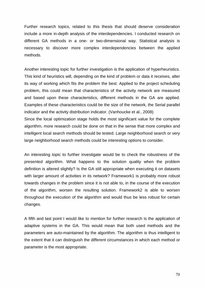
70

Further research topics, related to this thesis that should deserve consideration

include a more in-depth analysis of the interdependencies. I conducted research on

different GA methods in a one- or two-dimensional way. Statistical analysis is

necessary to discover more complex interdependencies between the applied

methods.

Another interesting topic for further investigation is the application of hyperheuristics.

This kind of heuristics will, depending on the kind of problem or data it receives, alter

its way of working which fits the problem the best. Applied to the project scheduling

problem, this could mean that characteristics of the activity network are measured

and based upon these characteristics, different methods in the GA are applied.

Examples of these characteristics could be the size of the network, the Serial parallel

indicator and the activity distribution indicator. (Vanhoucke et al., 2008)

Since the local optimization stage holds the most significant value for the complete

algorithm, more research could be done on that in the sense that more complex and

intelligent local search methods should be tested. Large neighborhood search or very

large neighborhood search methods could be interesting options to consider.

An interesting topic to further investigate would be to check the robustness of the

presented algorithm. What happens to the solution quality when the problem

definition is altered slightly? Is the GA still appropriate when executing it on datasets

with larger amount of activities in its network? Framework1 is probably more robust

towards changes in the problem since it is not able to, in the course of the execution

of the algorithm, worsen the resulting solution. Framework2 is able to worsen

throughout the execution of the algorithm and would thus be less robust for certain

changes.

A fifth and last point I would like to mention for further research is the application of

adaptive systems in the GA. This would mean that both used methods and the

parameters are auto-maintained by the algorithm. The algorithm is thus intelligent to

the extent that it can distinguish the different circumstances in which each method or

parameter is the most appropriate.

71

VI. References Ahuja R., Ergun Ö., Orlin J.B. and Punnen A.P. (2002) A survey of very largescale

neighborhood search techniques. Discrete Applied Mathematics, 123:

75–102

Association of Project Management January 1995 (version 2), Body of Knowledge

(BoK) Revised

Atkinson R. (1999), Project management: cost, time and quality, two best guesses

and a phenomenon, its time to accept other success criteria, Edition of book,

Great Britain: Elsevier Science Ltd and IPMA, p. 337-342.

Bäck T. (1993) Optimal mutation rates in genetic search. in Proceedings of the Fifth

International Conference on Genetic Algorithms. pp. 2-8.

Brucker P., Drexl A., Möhring R., Neumann K. and Pesch E. (1999)

Resourceconstrained project scheduling: notation, classi_cation, models, and

methods. Euro-pean Journal of Operational Research, 112:3-41.

Burgess A. R., Killebrew, J. B., (1962). “Variation in Activity Level on a

Cyclic Arrow Diagram”, Industrial Engineering, March-April, pp. 76-83.

Cottrell W. (1999) Simplified program evaluation and review technique (PERT). J.

Constr. Eng. Manage. , 125 (1), 16–22

Dawson C., Dawson R. (1995) Generalised activity-on-the-node networks for

managing uncertainty in projects. International Journal of Project

Management, 13, pp. 353–362

De Jong K. (1975) An analysis of the behavior of a class of genetic adaptive

systems, Dept. Comput. Sci., Univ. Michigan

72

Demeulemeester E. (1995) Minimizing resource availability costs in time-limited

Project networks. Management Science, Vol. 41, No. 10, 1590-1598

Elmaghraby S.E., (1977) Activity networks - Project planning and control by network

models, Wiley Interscience, New York.

Elmaghraby S. (1995). Activity nets: A guided tour through some recent

developments. European Journal of Operational Research, 82:383-408.

Eshelman L., Schaffer J.D. (1992). Real-Coded Genetic Algorithms and

IntervalSchemata. In L Darrel Whitley (ed), Foundations of Genetic

Algorithms 2. San Mateo, CA, Morgan Kaufmann Publishers.

Guldemond T., Hurink J., Paulus J., and Schutten J. (2008). Time-constrained

project scheduling. Journal of Scheduling, 11:137-148.

Hartmann S. and Briskorn D. (2010). A survey of variants and extensions of the

resource-constrained project scheduling problem. European Journal of

Operational Research, 207:1-15.

Herroelen W., Demeulemeester E. and De Reyck B., (1997) Resource-constrained

project scheduling – A survey of recent developments, Computers and

Operations Research, 25 (4), 279-302

Herroelen W., de Reyck B., Demeulemeester E. (1998) Resource-constrained

project scheduling: A survey of recent developments, Computers and

Operations Research 25 (4) 279–302.

Herroelen W., Demeulemeester E. and De Reyck B., (1999) An integrated

classification scheme for resource scheduling. DTEW Research Report 9905,

1-16

Holland J.R. (1975). Adaptation in natural and artificial systems. Ann Arbor, MI:

University of Michigan Press.

73

Icmeli 0., Erengiic S. and Zappe I. (1993) Project scheduling problems: a survey,

International Journal of Production and Operations Management, 13, 80-91.

Lin W., Lee W., Hong T. (2003) Adapting crossover and mutation rates in genetic

algorithms J Info Sci Eng, 19 (5), pp. 889–903

Luke S., Spector L. (1998) A revised comparison of crossover and mutation in

genetic programming, Proc. 3rd Annual Genetic Programming Conf., pp.208

213 1998

Maenhout B. and Vanhoucke M. (2010). Branching strategies in a branch-and-price

approach for a multiple objective nurse scheduling problem. Journal of

Scheduling, 13:77-93.

Maenhout B. and Vanhoucke M. (2014). An exact algorithm for an integrated project

staffing problem with a homogeneous workforce. Working paper

Magalhães J., Mendes A. (2013) Comparative Study of Crossover Operators for

Genetic Algorithms to Solve the Job Shop scheduling Problem, WSEAS

Transactions on computers, Vol. 12, No. 4, pp. 164-173.

Malcolm D., Roseboom J., Clark C. and Frazar W. (1959) Application of a Technique

for Research and Development Program Evaluation. Operations Research,

Vol. 7, pp. 646--669.

Muller L (2009) An adaptive large neighborhood search algorithm for the

Resourceconstrained project scheduling problem.

InMIC 2009: The VIII Metaheuristics International Conference, 2009.

Neumann K., Zimmermann J. (1999) Methods for resource-constrained project

scheduling problem with regular and nonregular objective functions and

schedule-dependent time windows, in: Weglarz [193], pp. 261–288.

74

Noever D. and Baskaran S. (1992) Steady State vs. Generational Genetic

Algorithms: A Comparison of Time Complexity and Convergence Properties.

Santa Fe Institute preprint series, 92-07-032.

Palpant M., Artigues C. C. and Michelon P. (2004) LSSPER: Solving the

Resourceconstrained project scheduling problem with large neighbourhood

search. Annals of Operations Research, 131:237–257, 2004.

Pisinger D., Ropke S. (2010) Large neighborhood search, Handbook of

Metaheuristics of International Series in Operations Research & Management

Science, vol. 146Springer, Boston, pp. 399–419

Project Management Institute (2004) A Guide to the Project Management Body of

Knowledge: PMBOK® Guide, 3rd Edition. Newtown Square, Pennsylvania,

Project Management Institute, p. 5.

Ropke S. and Pisinger D. (2006) A unified heuristic for a large class of vehicle routing

problems with backhauls.

European Journal of Operational Research, 171:750–775, 2006.

Sabuncuoglu I., Lejmi T. (1999) Scheduling for non regular performance measure

under the due window approach. Omega - International Journal of

Management Science, vol. 27, pp. 555-568

Sastry K., Goldberg D. (2001) Modeling tournament selection with replacement

using apparent added noise. Intelligent Engineering Systems Through

Artificial Neural Networks, vol. 11, pp.129 -134

Shaw P. (1998) Using constraint programming and local search methods to solve

vehicle routing problems. In CP-98 (Fourth International Conference on

Principles and Practice of Constraint Programming), volume 1520 of Lecture

Notes in Computer Science, pages 417–431, 1998.

75

Sivaraj R., Ravichandran T. (2011) A review of selection methods in genetic

algorithm, Int. J. Eng. Sci. Tech., 3, p. 3792

Spears W., Anand V., Ras Z. and Zemankova M (1991) A study of crossover

operators in genetic programming, Proc. 6th Int. Symp. Methodologies for

Intelligent Systems (ISMIS',91), pp.409 -418 :Springer-Verlag

Syswerda G. (1991) A Study of Reproduction in Generational and Steady-State

Genetic Algorithms. Rawlins, G.J.E., Foundations of genetic algorithms. San

Mateo, CA:Morgan Kaufmann Publishers.

Takahashi M., Kita H. (2001) A Crossover Operator Using Independent Component

Analysis for Real-Coded Genetic Algorithm, in Proceedings of the 2001

Congress on Evolutionary Computation, pp. 643-649

Turner J., Rodney (1993) The handbook of project-based management. McGraw-Hill,

London, 540p.

Vanhoucke M., Coelho J., Debels D., Maenhout B., Tavares L.V. (2008)

An evaluation of the adequacy of project network generators with

systematically sampled networks European Journal of Operational Research,

187 , pp. 511–524

Wall B. (1996) A Genetic Algorithm for Resource Constrained Scheduling, PhD

Thesis, Department of Mechanical Engineering, Massachusetts Institute of

Technology, USA.

Whitley D. (1989) The GENITOR algorithm and selective pressure. Proceedings of

the Third International Conference on Genetic Algorithms, pp. 116–121.

Morgan Kaufmann, San Mateo, CA.

76

VII. Appendices

Appendix A: Datasets

AN1

CP = 9 days

SPI = 0.11

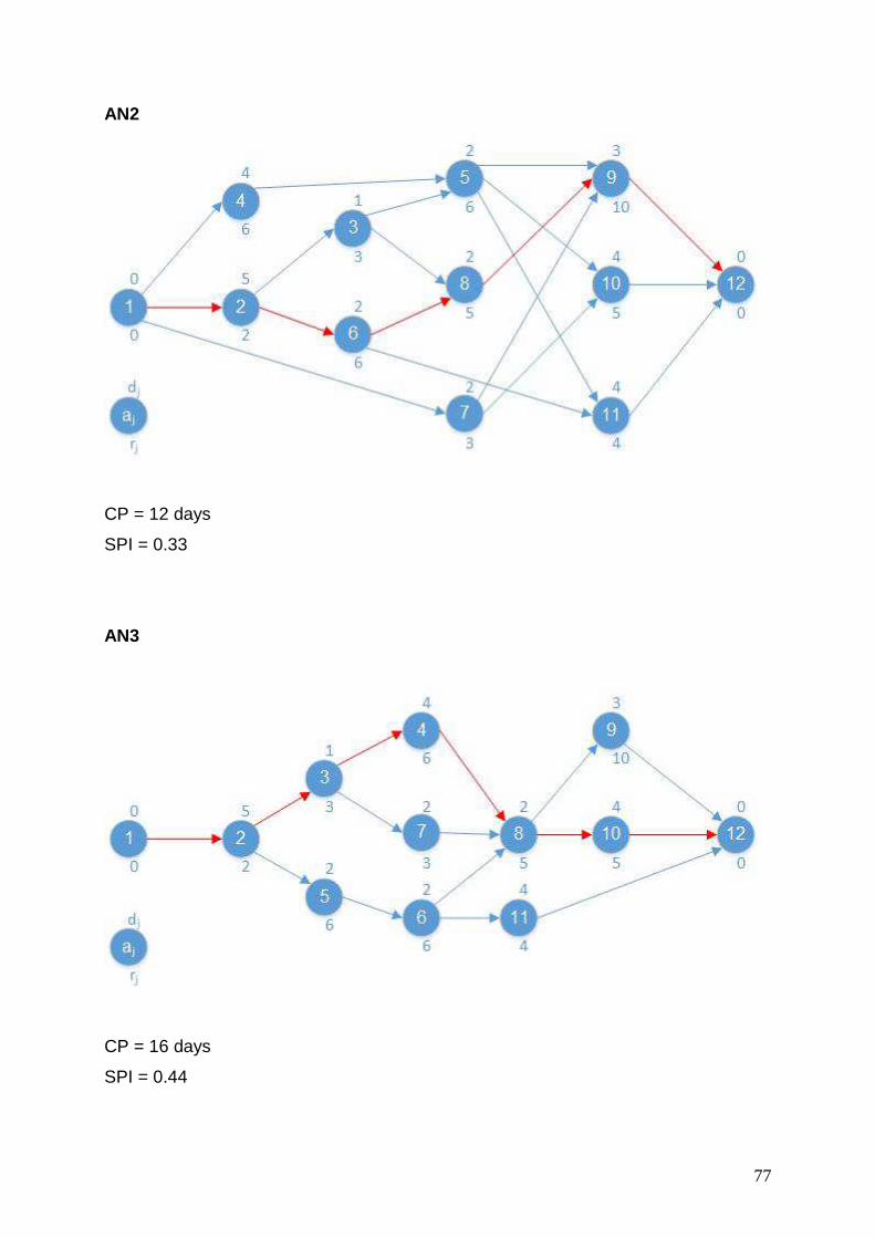
77

AN2

CP = 12 days

SPI = 0.33

AN3

CP = 16 days

SPI = 0.44

78

Appendix B: Method elimination in basic cycles

AN1 Framework1

Stage → Initialization Selection Operation Local Optimization Reinsert condition Doubles

Population management Cost

Phase ↓ I1a I1b I1c I2a I2b I2c I3a I3b I3c I3d I4 S1 S2 S3 S4 C1 C2 C3 C4 C5 C6 L1 L2 L3 L4 R1 R2 R3 R4 R5 R6 N Y P1 P2 P3 Base Case x x x x x x x x x x x x x x x x x x x x x x x x x x x x x x x x x x x x 400,10 1st Exclusion x x x x x x x x x x x x x x x x x x x x x 368,73 2nd Exclusion x x x x x x x x x x x x x x 363,96 Best X x x x x x x x x x x x 358,23 Best x x x x x x x 355,25

AN1 Framework2

Stage → Initialization Selection Operation Local Optimization Reinsert condition Doubles

Population management Cost

Phase ↓ I1a I1b I1c I2a I2b I2c I3a I3b I3c I3d I4 S1 S2 S3 S4 C1 C2 C3 C4 C5 C6 L1 L2 L3 L4 R1 R2 R3 R4 R5 R6 N Y P1 P2 P3 Base Case x x x x x x x x x x x x x x x x x x x x x x x x x x x x x x x x x x x x 400,67 1st Exclusion x x x x x x x x x x x x x x x x x x x 378,34 2nd Exclusion x x x x x x x x x x x x x 371,36 Best X x x x x x x x x x x 366,32 Best x x x x x x x 365,67

AN2 Framework1

Stage → Initialization Selection Operation Local Optimization Reinsert condition Doubles

Population management Cost

Phase ↓ I1a I1b I1c I2a I2b I2c I3a I3b I3c I3d I4 S1 S2 S3 S4 C1 C2 C3 C4 C5 C6 L1 L2 L3 L4 R1 R2 R3 R4 R5 R6 N Y P1 P2 P3 Base Case x x x x x x x x x x x x x x x x x x x x x x x x x x x x x x x x x x x x 402,06 1st Exclusion x x x x x x x x x x x x x x x x x x x 391,04 2nd Exclusion x x x x x x x x x x x x x x 388,91 Best X x x x x x x x x x x x 386,74 Best x x x x x x x 385,34

79

AN2 Framework2

Stage → Initialization Selection Operation Local Optimization Reinsert condition Doubles

Population management Cost

Phase ↓ I1a I1b I1c I2a I2b I2c I3a I3b I3c I3d I4 S1 S2 S3 S4 C1 C2 C3 C4 C5 C6 L1 L2 L3 L4 R1 R2 R3 R4 R5 R6 N Y P1 P2 P3 Base Case x x x x x x x x x x x x x x x x x x x x x x x x x x x x x x x x x x x x 403,51 1st Exclusion x x x x x x x x x x x x x x x x x x x x x x x x 389,67 2nd Exclusion x x x x x x x x x x x x x x x x x x x x x 389,09 Best X x x x x x x x x x x 387,03 Best x x x x x x x 386,29

AN3 Framework1

Stage → Initialization Selection Operation Local Optimization Reinsert condition Doubles

Population management Cost

Phase ↓ I1a I1b I1c I2a I2b I2c I3a I3b I3c I3d I4 S1 S2 S3 S4 C1 C2 C3 C4 C5 C6 L1 L2 L3 L4 R1 R2 R3 R4 R5 R6 N Y P1 P2 P3 Base Case x x x x x x x x x x x x x x x x x x x x x x x x x x x x x x x x x x x x 399,82 1st Exclusion x x x x x x x x x x x x x x x x x x x x x 391,16 2nd Exclusion x x x x x x x x x x x x x x x x 386,60 Best X x x x x x x x x x x 384,42 Best x x x x x x 384,29

AN3 Framework2

Stage → Initialization Selection Operation Local Optimization Reinsert condition Doubles

Population management Cost

Phase ↓ I1a I1b I1c I2a I2b I2c I3a I3b I3c I3d I4 S1 S2 S3 S4 C1 C2 C3 C4 C5 C6 L1 L2 L3 L4 R1 R2 R3 R4 R5 R6 N Y P1 P2 P3 Base Case x x x x x x x x x x x x x x x x x x x x x x x x x x x x x x x x x x x x 404,79 1st Exclusion x x x x x x x x x x x x x x x x x x x x 388,14 2nd Exclusion x x x x x x x x x x x x x x 388,19 Best X x x x x x x x x x x 387,83 Best x x x x x x x 386,00

80

Appendix C: Cost evolutions of basic cycles

AN1 Framework 1

Phase Average Min Max Base Case 400,1 355 554 1st Exclusion 368,73 351 390 2nd Exclusion 363,96 354 379 Best X 358,23 352 374 Best 355,25 352 359

AN1 Framework 2

Phase Average Min Max Base Case 400,67 361 414 1st Exclusion 378,34 352 403 2nd Exclusion 371,36 355 405 Best X 366,32 355 396 Best 365,67 355 382

Total Cost evolution

350

400

450

500

550

Base Case 1stExclusion

2ndExclusion

Best X Best

Phase

Tot

al C

ost

Average

Min

Max

81

AN2 Framework 1

Phase Average Min Max Base Case 402,06 383 450 1st Exclusion 391,04 380 410 2nd Exclusion 388,91 378 401 Best X 386,74 373 405 Best 385,34 373 400

Total Cost evolution

350

360

370

380

390

400

410

Base Case 1stExclusion

2ndExclusion

Best X Best

Phase

Tot

al C

ost

Average

Min

Max

Total Cost evolution

370

380

390

400

410

420

430

440

450

460

Base Case 1stExclusion

2ndExclusion

Best X Best

Phase

Tot

al C

ost

Average

Min

Max

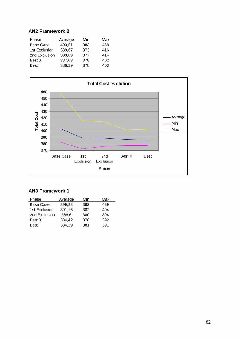
82

AN2 Framework 2

Phase Average Min Max Base Case 403,51 383 458 1st Exclusion 389,67 373 416 2nd Exclusion 389,09 377 414 Best X 387,03 378 402 Best 386,29 378 403

AN3 Framework 1

Phase Average Min Max Base Case 399,82 382 439 1st Exclusion 391,16 382 404 2nd Exclusion 386,6 380 394 Best X 384,42 378 392 Best 384,29 381 391

Total Cost evolution

370

380

390

400

410

420

430

440

450

460

Base Case 1stExclusion

2ndExclusion

Best X Best

Phase

Tot

al C

ost

Average

Min

Max

83

AN3 Framework 2

Phase Average Min Max Base Case 404,79 383 514 1st Exclusion 388,14 378 404 2nd Exclusion 388,19 378 400 Best X 387,83 378 400 Best 386 382 390

Total Cost evolution

375

385

395

405

415

425

435

Base Case 1stExclusion

2ndExclusion

Best X Best

Phase

Tot

al C

ost

Average

Min

Max

Total Cost evolution

375

395

415

435

455

475

495

515

Base Case 1stExclusion

2ndExclusion

Best X Best

Phase

Tot

al C

ost

Average

Min

Max

84

Appendix D: Observation link AVGSQDEV – Total cost

All project lengths

Project length = 8

Project Length =11

Average Squared deviation - Objective

170

190

210

230

250

270

0 50 100 150 200 250 300

Average Squared deviation

Obj

ectiv

e

Average Squared deviation - Objective

170

190

210

230

250

270

0 50 100 150 200 250 300

Average Squared deviation

Obj

ectiv

e

Average Squared deviation - Objective

170

190

210

230

250

270

0 20 40 60 80 100 120 140 160 180 200

Average Squared deviation

Obj

ectiv

e

85

Project Length = 14

Project Length = 17

Project Length = 20

Average Squared deviation - Objective

170

190

210

230

250

270

0 20 40 60 80 100 120 140

Average Squared deviation

Obj

ectiv

e

Average Squared deviation - Objective

170

190

210

230

250

270

0 10 20 30 40 50 60 70 80 90 100

Average Squared deviation

Obj

ectiv

e

Average Squared deviation - Objective

170

190

210

230

250

270

0 10 20 30 40 50 60 70 80

Average Squared deviation

Obj

ectiv

e