
Getting Started Manual - XP Solutions
291
STORMWATER MANAGEMENT MODEL storm GETTING STARTED MANUAL
Transcript of Getting Started Manual - XP Solutions
STORMWATER MANAGEMENT MODEL
storm
GETTING STARTED MANUAL
Copyright
© 2014 XP Solutions. All rights reserved. No part of this publication may be reproduced in any form by any means without the written permission of XP Solutions. XP-STORM and xpstorm are trademarks of XP Solutions. Other brand and product names are trademarks or registered trademarks of their respective holders.
Software License Notice
Your License Agreement, which is included with this product, specifies the permitted and prohibited uses of the product. Any unauthorized duplication or use of xpstorm in whole or in part, in print or in any other storage and retrieval system is forbidden.
Disclaimer
The XP environment and its documentation have been released by XP Solutions as a proprietary model and as such are not available to unauthorized users.
The authors and XP Solutions, although taking every care to provide error free code, because of the complexity and nature of this type of software, cannot make explicit warranties as to the documentation, function, or performance of the model. Should any errors be found during program operation the user should direct the problem to XP Solutions where every effort will be made to quickly resolve the problem. Although the data checking facilities of the model are extensive, incorrect results may be produced if poor or inappropriate data are entered.
Users are expected to make the final evaluation as to the usefulness of the model for their purposes. He or she must use his or her own engineering judgment as to the applicability of the model to the job at hand and perform reasonable engineering checks on the data and results. XP Solutions cannot assume responsibility for model output, interpretation or usage.
No portion of this document may be reproduced in any form without the express written consent of XP Solutions.

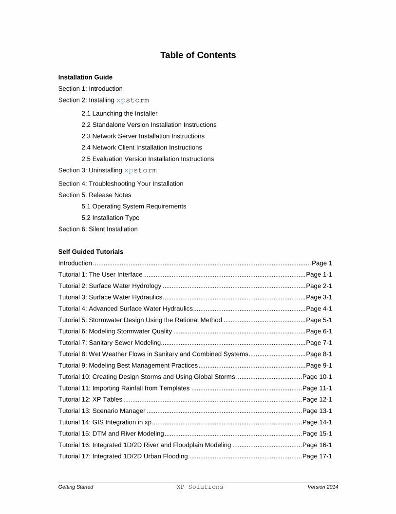
Table of Contents
Installation Guide
Section 1: Introduction
Section 2: Installing xpstorm
2.1 Launching the Installer
2.2 Standalone Version Installation Instructions
2.3 Network Server Installation Instructions
2.4 Network Client Installation Instructions
2.5 Evaluation Version Installation Instructions
Section 3: Uninstalling xpstorm
Section 4: Troubleshooting Your Installation
Section 5: Release Notes
5.1 Operating System Requirements
5.2 Installation Type
Section 6: Silent Installation
Self Guided Tutorials
Introduction .......................................................................................................................... Page 1
Tutorial 1: The User Interface ........................................................................................... Page 1-1
Tutorial 2: Surface Water Hydrology ................................................................................ Page 2-1
Tutorial 3: Surface Water Hydraulics ................................................................................ Page 3-1
Tutorial 4: Advanced Surface Water Hydraulics ............................................................... Page 4-1
Tutorial 5: Stormwater Design Using the Rational Method .............................................. Page 5-1
Tutorial 6: Modeling Stormwater Quality .......................................................................... Page 6-1
Tutorial 7: Sanitary Sewer Modeling................................................................................. Page 7-1
Tutorial 8: Wet Weather Flows in Sanitary and Combined Systems ................................ Page 8-1
Tutorial 9: Modeling Best Management Practices ............................................................ Page 9-1
Tutorial 10: Creating Design Storms and Using Global Storms ..................................... Page 10-1
Tutorial 11: Importing Rainfall from Templates .............................................................. Page 11-1
Tutorial 12: XP Tables .................................................................................................... Page 12-1
Tutorial 13: Scenario Manager ....................................................................................... Page 13-1
Tutorial 14: GIS Integration in xp .................................................................................... Page 14-1
Tutorial 15: DTM and River Modeling ............................................................................. Page 15-1
Tutorial 16: Integrated 1D/2D River and Floodplain Modeling ....................................... Page 16-1
Tutorial 17: Integrated 1D/2D Urban Flooding ............................................................... Page 17-1
Getting Started XP Solutions Version 2014

1. Installation Guide Introduction
Welcome to XP Solutions’s xpstorm stormwater and wastewater decision support system. xpstorm is a link-node model that performs hydrologic, hydraulic and quality analysis of stormwater and wastewater drainage systems including sewage treatment plants, water quality control devices and Best Management Practices (BMP’s). This software package utilizes sophisticated graphical tools together with associated Geographical Information Systems and CAD. xpstorm is a full 32 bit software package for Windows XP, Vista, 7 (32 and 64 bits), 8 as well as Windows 2008, 2008 R2, 2012, and 2012 R2 for the server versions.
xpstorm may be used to model the full hydrologic cycle from stormwater and wastewater flow and pollutant generation to simulation of the hydraulics in any combined system of open and/or closed conduits with any boundary conditions.
This manual details the installation of xpstorm. If you follow all steps outlined in the following pages you will have a successful installation. If you have any problems throughout the course of your installation please consult the Troubleshooting Section (Section 4) in this manual or contact XP Solutions Technical Support.
To maximize your investment, XP Solutions would encourage your participation at one of their regular detailed training workshops. The schedule for public workshops can be found at www.xpsolutions.com.
The tutorials that follow the introductory and installation sections will provide you a basic introduction to modelling applications of xpstorm. The set of tutorials will also act as an overview to most of the model building and results presentation tools. The graphic images and the text instructions have been based on installing xpstorm in the default folder C:\Program Files (x86)\XP Solutions\xpstorm2014. This root of the installation may be different in your case and therefore you should make any necessary adjustments when searching for files to complete the tutorials.
Regardless of the selected root folder the templates, work, and samples folder will be located from the main xpstorm folder.
Page 1
Page 2
2. Installing xpstorm
2.1 Launching the Installer
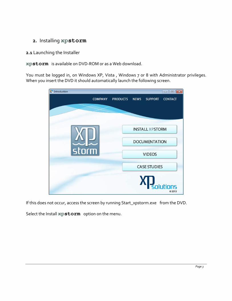
xpstorm is available on DVD-ROM or as a Web download.
You must be logged in, on Windows XP, Vista , Windows 7 or 8 with Administrator privileges. When you insert the DVD it should automatically launch the following screen.
If this does not occur, access the screen by running Start_xpstorm.exe from the DVD.
Select the Install xpstorm option on the menu.
Page 3
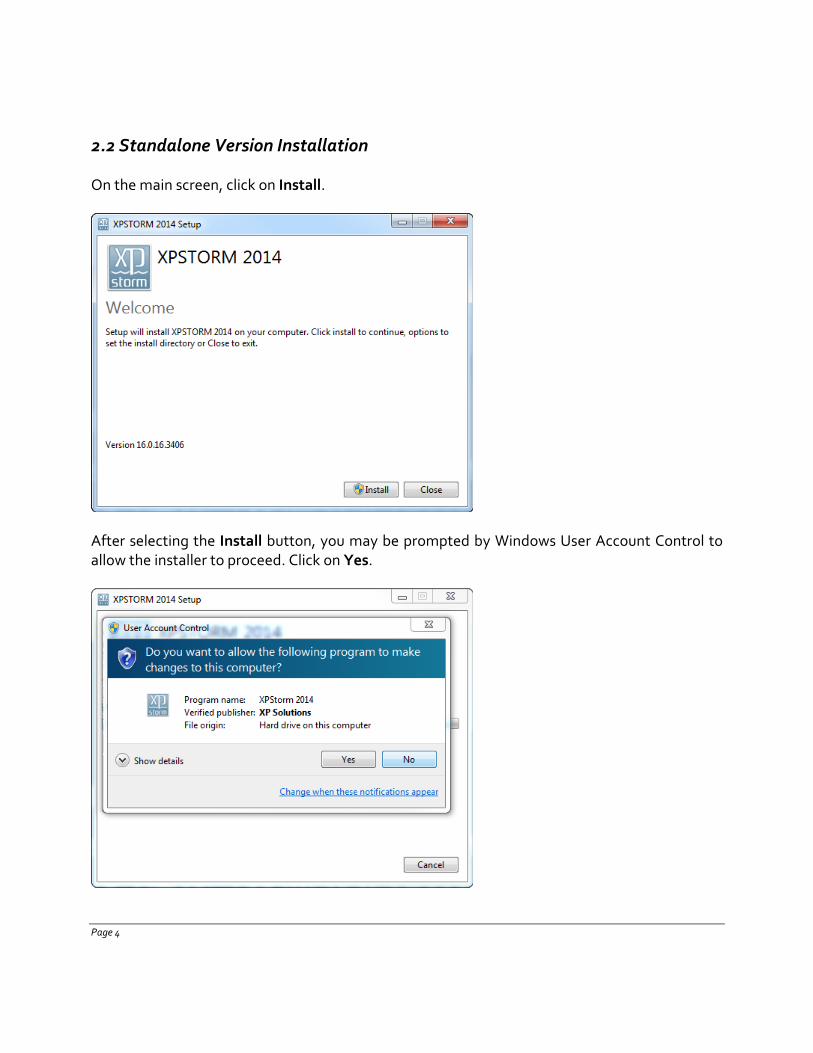
2.2 Standalone Version Installation
On the main screen, click on Install.
After selecting the Install button, you may be prompted by Windows User Account Control to allow the installer to proceed. Click on Yes.
Page 4

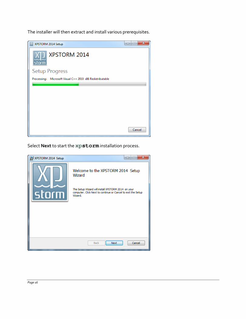
The installer will then extract and install various prerequisites.
Select Next to start the xpstorm installation process.
Page 5
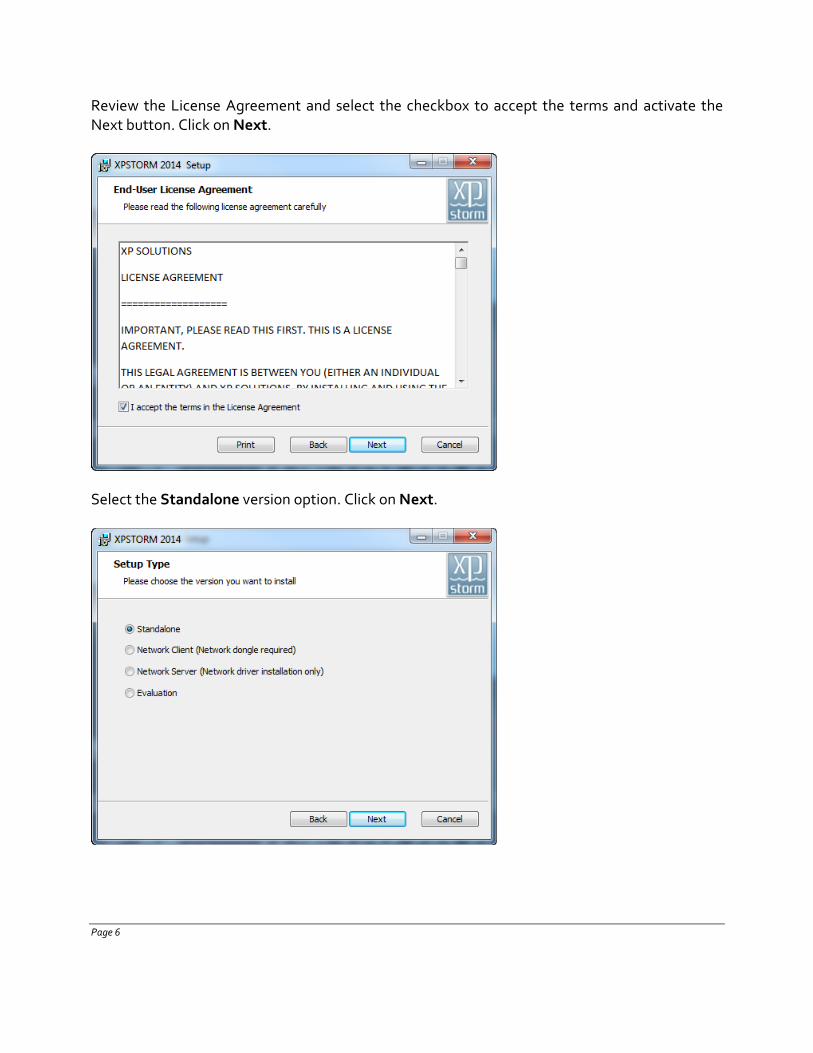
Review the License Agreement and select the checkbox to accept the terms and activate the Next button. Click on Next.
Select the Standalone version option. Click on Next.
Page 6
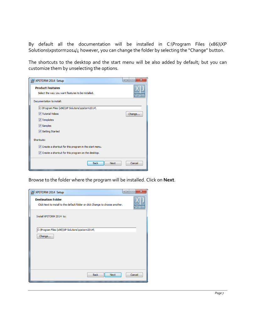
By default all the documentation will be installed in C:\Program Files (x86)\XP Solutions\xpstorm2014\; however, you can change the folder by selecting the “Change” button.
The shortcuts to the desktop and the start menu will be also added by default; but you can customize them by unselecting the options.
Browse to the folder where the program will be installed. Click on Next.
Page 7
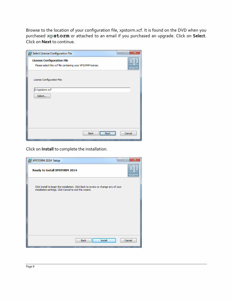
Browse to the location of your configuration file, xpstorm.xcf. It is found on the DVD when you purchased xpstorm or attached to an email if you purchased an upgrade. Click on Select. Click on Next to continue.
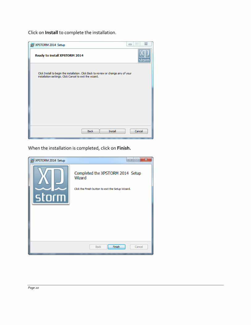
Click on Install to complete the installation.
Page 8
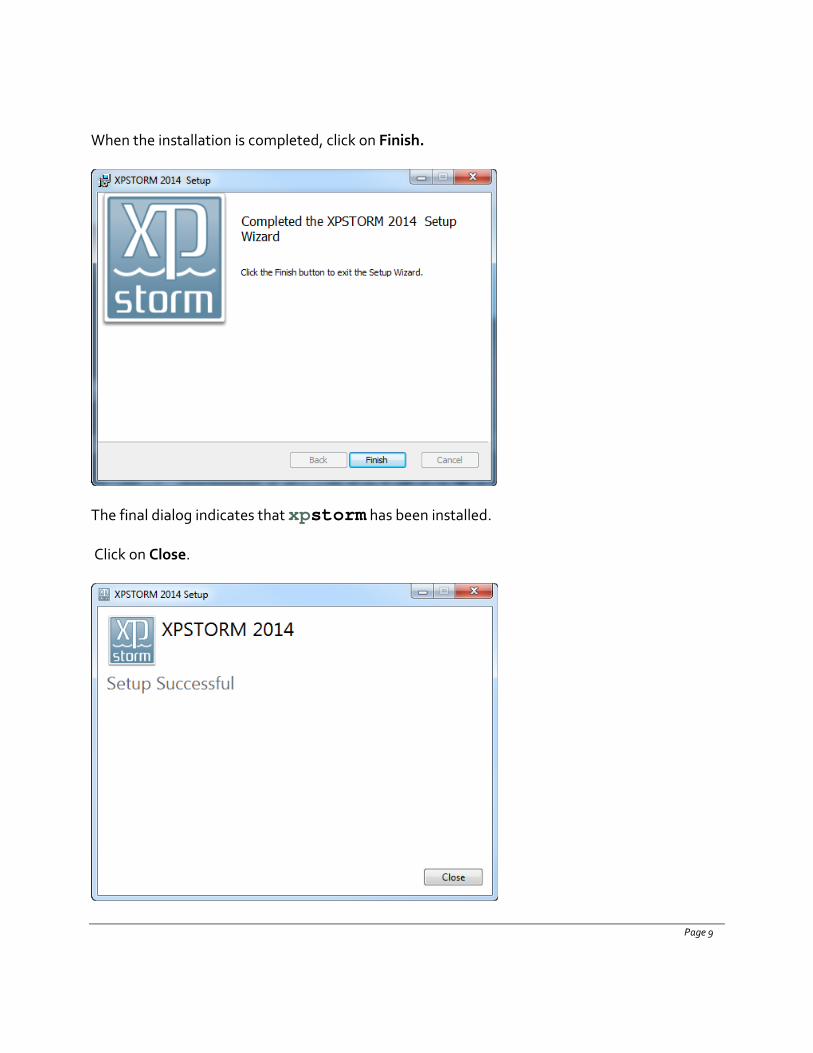
When the installation is completed, click on Finish.
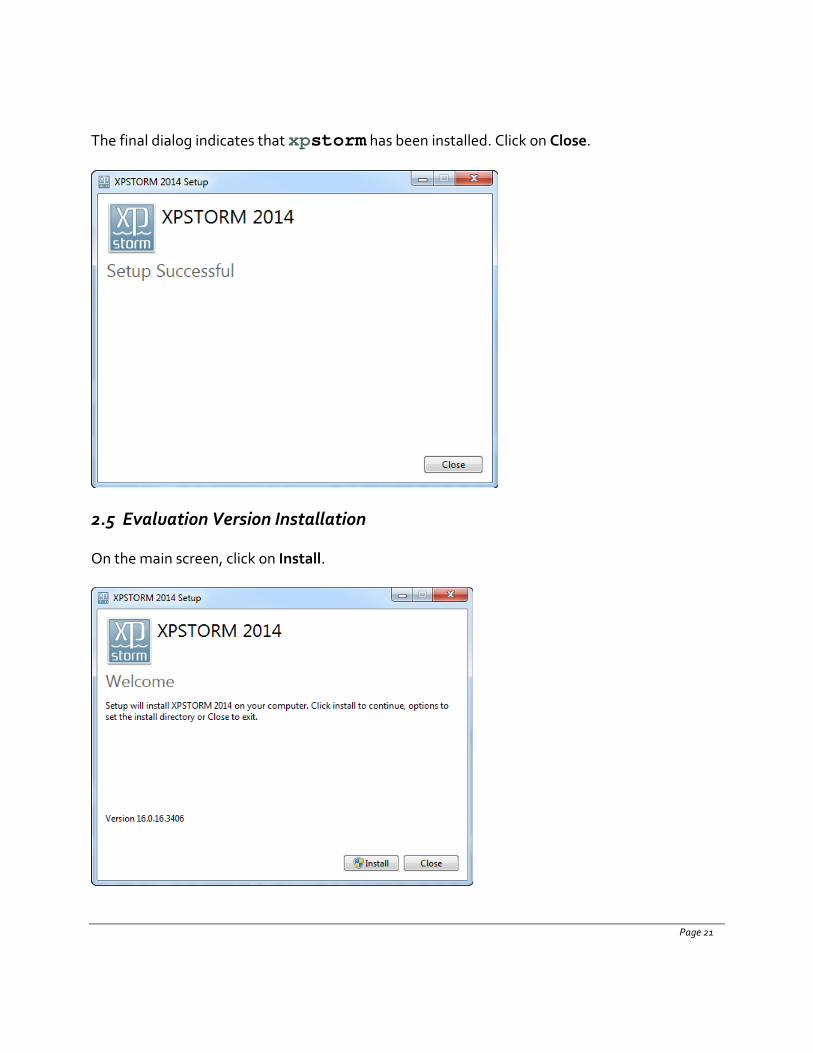
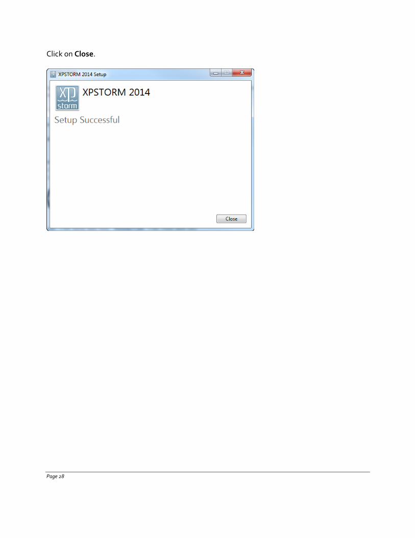
The final dialog indicates that xpstorm has been installed.
Click on Close.
Page 9
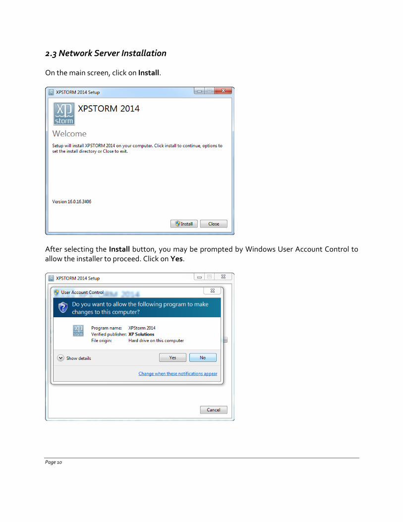
2.3 Network Server Installation
On the main screen, click on Install.
After selecting the Install button, you may be prompted by Windows User Account Control to allow the installer to proceed. Click on Yes.
Page 10
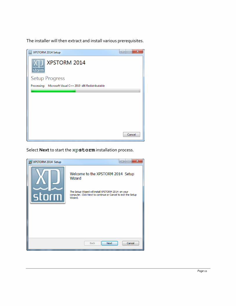
The installer will then extract and install various prerequisites.
Select Next to start the xpstorm installation process.
Page 11

Review the License Agreement and select the checkbox to accept the terms and activate the Next button. Click on Next.
Select the Network Server version option. Click on Next.
Page 12
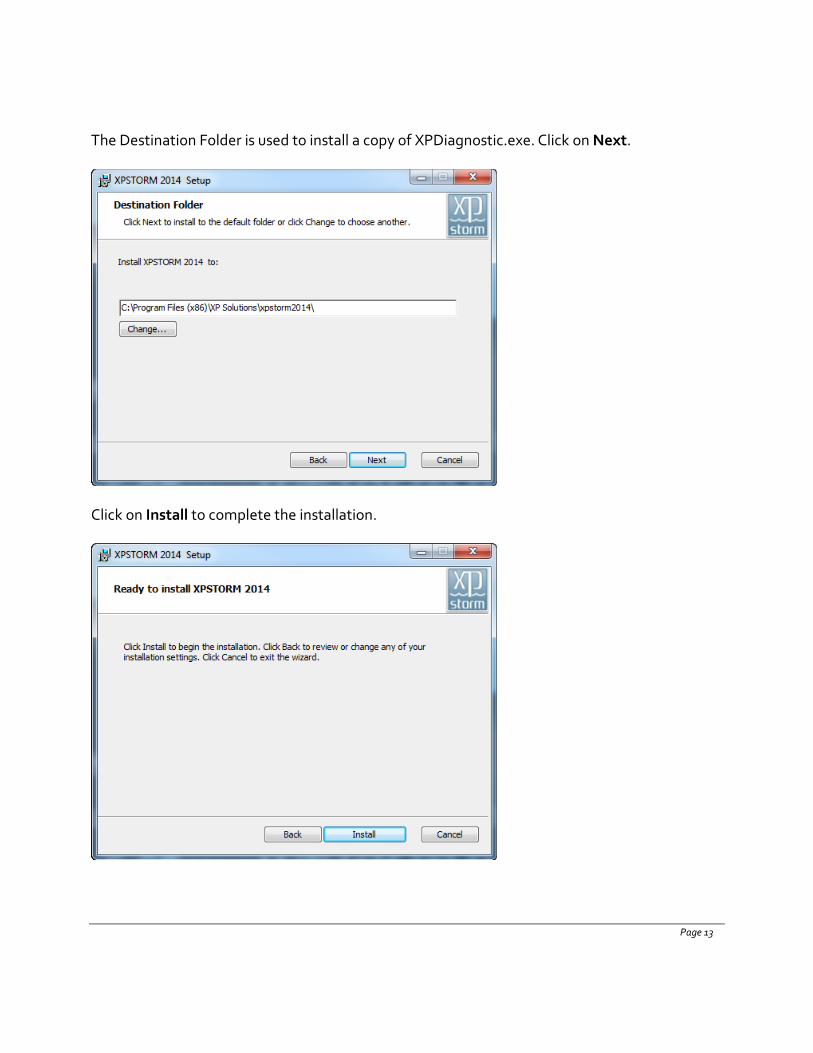
The Destination Folder is used to install a copy of XPDiagnostic.exe. Click on Next.
Click on Install to complete the installation.
Page 13
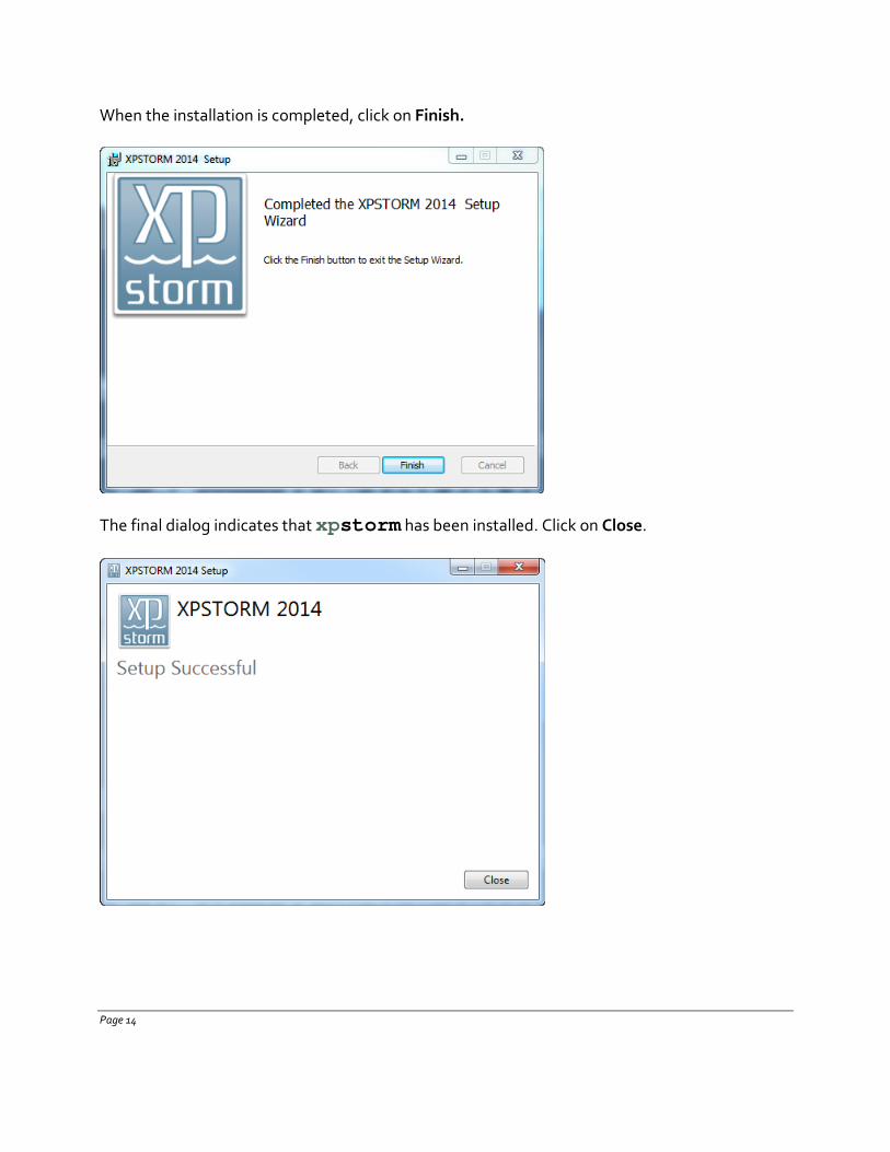
When the installation is completed, click on Finish.
The final dialog indicates that xpstorm has been installed. Click on Close.
Page 14
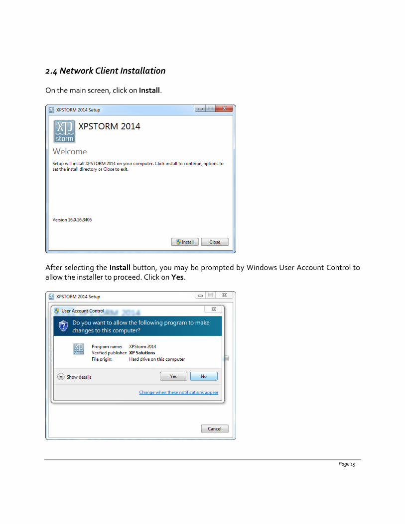
2.4 Network Client Installation
On the main screen, click on Install.
After selecting the Install button, you may be prompted by Windows User Account Control to allow the installer to proceed. Click on Yes.
Page 15
The installer will then extract and install various prerequisites.
Select Next to start the xpstorm installation process.
Page 16
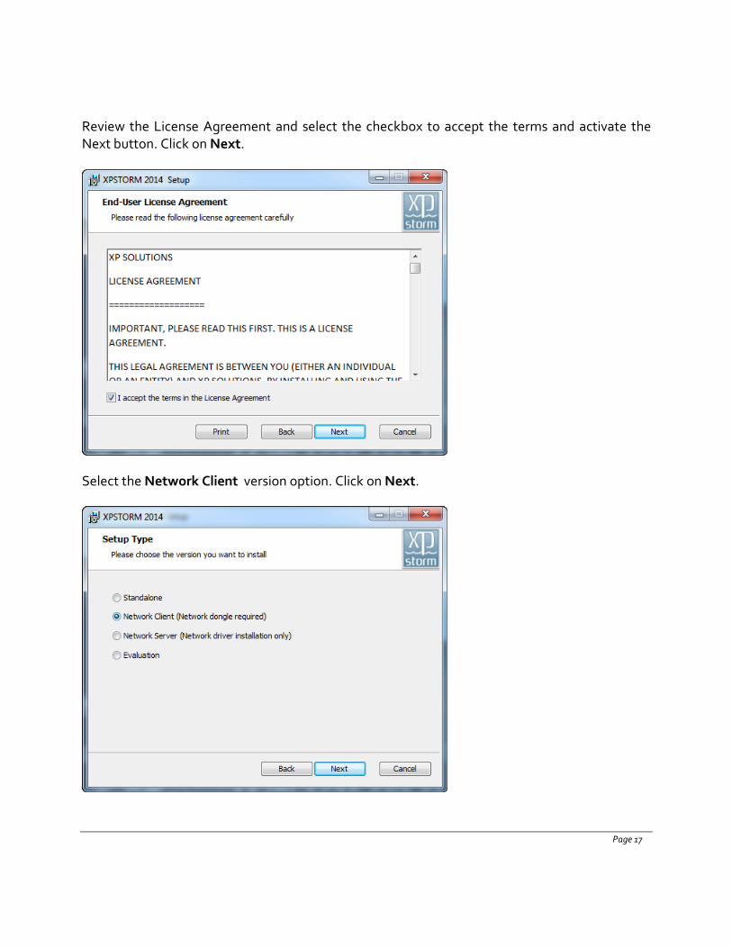
Review the License Agreement and select the checkbox to accept the terms and activate the Next button. Click on Next.
Select the Network Client version option. Click on Next.
Page 17
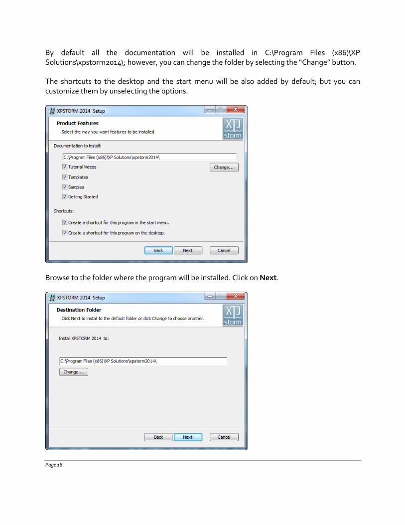
By default all the documentation will be installed in C:\Program Files (x86)\XP Solutions\xpstorm2014\; however, you can change the folder by selecting the “Change” button.
The shortcuts to the desktop and the start menu will be also added by default; but you can customize them by unselecting the options.
Browse to the folder where the program will be installed. Click on Next.
Page 18
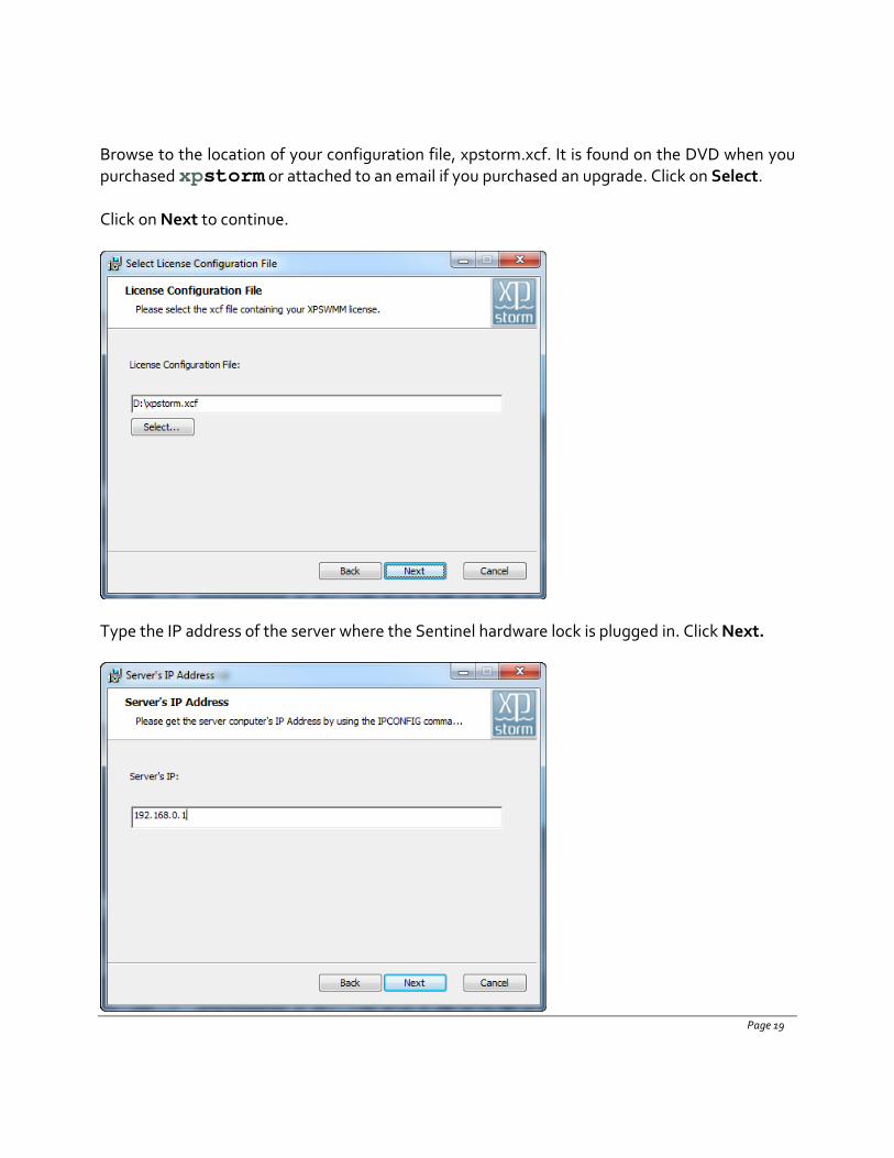
Browse to the location of your configuration file, xpstorm.xcf. It is found on the DVD when you purchased xpstorm or attached to an email if you purchased an upgrade. Click on Select.
Click on Next to continue.
Type the IP address of the server where the Sentinel hardware lock is plugged in. Click Next.
Page 19
Click on Install to complete the installation.
When the installation is completed, click on Finish.
Page 20
The final dialog indicates that xpstorm has been installed. Click on Close.
2.5 Evaluation Version Installation
On the main screen, click on Install.
Page 21
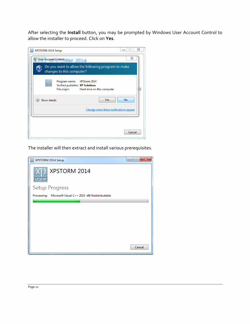
After selecting the Install button, you may be prompted by Windows User Account Control to allow the installer to proceed. Click on Yes.
The installer will then extract and install various prerequisites.
Page 22
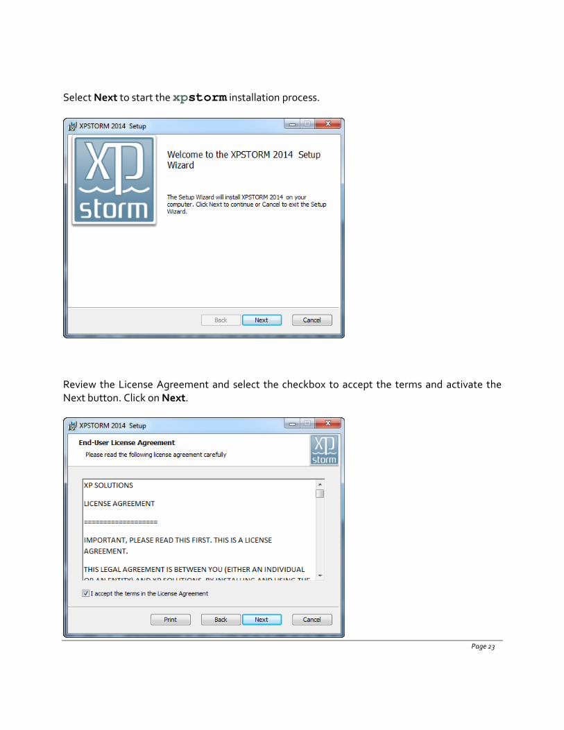
Select Next to start the xpstorm installation process.
Review the License Agreement and select the checkbox to accept the terms and activate the Next button. Click on Next.
Page 23
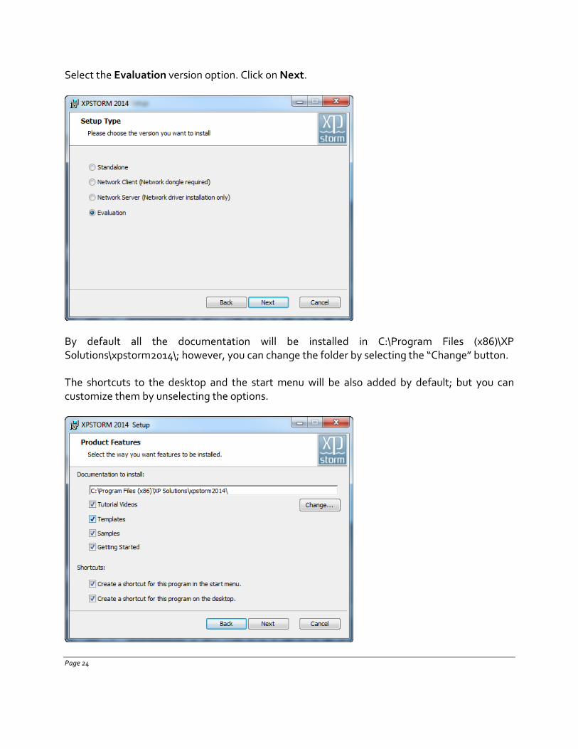
Select the Evaluation version option. Click on Next.
By default all the documentation will be installed in C:\Program Files (x86)\XP Solutions\xpstorm2014\; however, you can change the folder by selecting the “Change” button.
The shortcuts to the desktop and the start menu will be also added by default; but you can customize them by unselecting the options.
Page 24
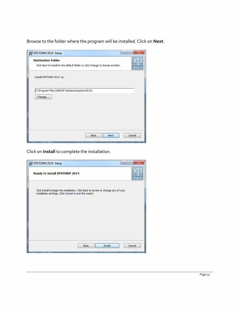
Browse to the folder where the program will be installed. Click on Next.
Click on Install to complete the installation.
Page 25
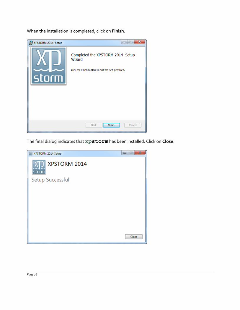
When the installation is completed, click on Finish.
The final dialog indicates that xpstorm has been installed. Click on Close.
Page 26
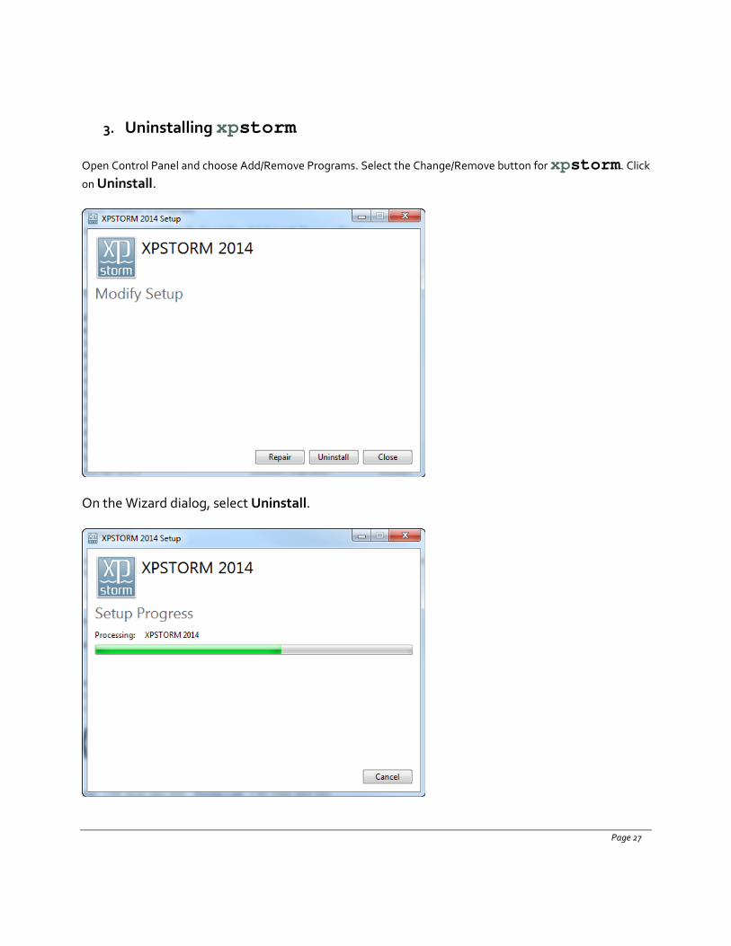
3. Uninstalling xpstorm
Open Control Panel and choose Add/Remove Programs. Select the Change/Remove button for xpstorm. Click
on Uninstall.
On the Wizard dialog, select Uninstall.
Page 27
Click on Close.
Page 28
4. Troubleshooting Your Installation
Error 3: Dongle not found.
Solution 1: The license configuration file was not found in the xpstorm directory or is read only. Find the xpstorm.xcf file with the correct version number for the version of xpstorm that you are installing. The file may have been attached to an e-mail from XP Solutions announcing your product eligibility or can be found on the root directory of the installation DVD.
Copy and paste the file into your xpstorm directory.
It is important to mention that in previous versions of xpstorm, the configuration file had the extension *.cnf.
Solution 2: The license configuration file in the xpstorm directory is read only. Check the properties of the file and make it read/write.
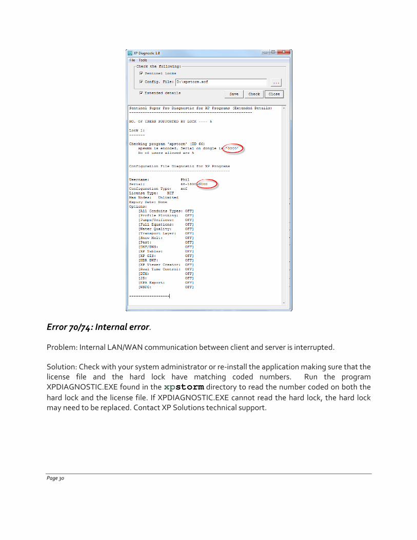
Solution 3: The license configuration file does not have the correct license number for the Sentinel hard lock that you are using. The numbers coded on the hard lock and in the license file must match.
1. Run the program XPDIAGNOSTIC.EXE found in the xpstorm directory to read the number coded on both the hard lock and the license file.
2. Find and install a matching pair of hard lock and license files. 3. Copy and paste the file into your xpstorm directory or re-install the application.
Page 29
Error 70/74: Internal error.
Problem: Internal LAN/WAN communication between client and server is interrupted.
Solution: Check with your system administrator or re-install the application making sure that the license file and the hard lock have matching coded numbers. Run the program XPDIAGNOSTIC.EXE found in the xpstorm directory to read the number coded on both the hard lock and the license file. If XPDIAGNOSTIC.EXE cannot read the hard lock, the hard lock may need to be replaced. Contact XP Solutions technical support.
Page 30
Try to install xpstorm again with the log activated
1. Open the command line (Start->Run, type cmd, click OK) 2. Install XPSTORM by typing one of the following lines
xpstorm2014.exe /L "d:\mylog.log" xpstorm2014.exe /log d:/mylog.log
3. Please send us by e-mail the file generated in the installation if you still face the problem.
Error uninstalling xpstorm
Problem. The XP Products register some components in the Windows Registry Editor, therefore, if you remove some files without removing them also from the registry or if you do not uninstall the product properly; there will be a mismatch between the files in the registry and the system.
Solution1. Run the msicuu.exe tool attached in the \Disc Image\Resources\technical support folder to make sure that the software will be completely deleted from your system. This program usually forces the software to uninstall and removes all registries. Run msicuu.exe with Administrator permission, select xpstorm 2014 from the list display and
click on the Uninstall button.
Solution 2. Open the \Disc Image\Resources\technical support \remove-registry-xpstorm2014.reg file; run it with administrator permissions and then try to reinstall xpstorm 2014.
For the Sentinel drivers, we usually ask the client to install the SSD Cleanup utility from this link http://www.safenet-inc.com/support-downloads/sentinel-drivers/
Page 31
5. xpstorm Release Notes
5.1 Operating System Requirements
This installer for xpstorm 2014 will run on:
• Windows XP • Windows Vista • Windows 7 • Windows 8
All of above operating systems are compatible in both 32 and 64 bits.
5.2 Installation Type
xpstorm is available in three installations:
• Standalone - requires Sentinal lock and client specific configuration file.
• Network - requires Sentinal lock and client specific configuration file.
• Evaluation/Demo - Software Protection - 30 day ready to try license, starts in demo mode and can be upgraded with electronic key to and evaluation configuration of 5 nodes, key printing, export, and saving disabled in demo but saving and printing available in the evaluation.
Note: Please report any problems to [email protected]
Page 32
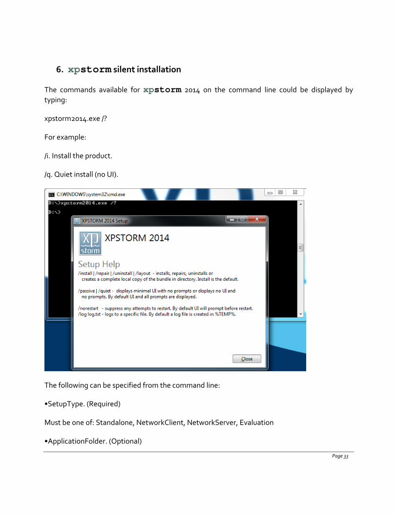
6. xpstorm silent installation
The commands available for xpstorm 2014 on the command line could be displayed by typing:
xpstorm2014.exe /?
For example:
/i. Install the product.
/q. Quiet install (no UI).
The following can be specified from the command line:
•SetupType. (Required)
Must be one of: Standalone, NetworkClient, NetworkServer, Evaluation
•ApplicationFolder. (Optional)
Page 33
The folder in which the application will be installed to. If not set, it will install to the default location (e.g. C:\Program Files (x86)\XP Solutions\xpstorm2014).
•LicenseFile. (Required for Standalone and Network Client setup types.)
The path to the xcf license configuration file.
•ServerAddress. (Required for NetworkClient)
The IP address of the server that has Sentinel network dongle.
Examples of using the installer from the command line:
Standalone (Sentinel):
xpstorm2014.exe /i /q SetupType=Standalone ApplicationFolder=C:\XPS\xpstorm2014 LicenseFile=C:\XP\xpstorm.xcf
Network Client:
xpstorm2014.exe /i /q SetupType=NetworkClient ApplicationFolder=C:\XPS\xpstorm2014 LicenseFile=C:\XP\xpstorm.xcf ServerAddress=192.168.1.1
Network Server:
xpstorm2014.exe /i /q SetupType=NetworkServer ApplicationFolder=C:\XPS\xpstorm2014
Evaluation:
xpstorm2014.exe /i /q SetupType=Evaluation ApplicationFolder=C:\XPS\xpstorm2014
Page 34

The xp Graphical User Interface The xp graphical user interface (GUI) utilizes the current Windows, Icons, Menus and Pointing device technology in a state-of-the-art intuitive user environment. This environment consists of:
• A window with a series of menus along the top of the screen used for controlling operation of the program and a status bar at the bottom. The window displays a plan view of the active xp model.
• Several tool strips containing icons for file operation, object creation/manipulation and short cuts to menu commands.
• Panels for displaying data or managing network display that either float or are docked to an edge of the screen.
The xp interface may be used to create a new hydrology and hydraulics network as well as to edit an existing one. The user interface is object-oriented which means the user selects the object, and then selects the operation to perform on it. A user first selects an object or range of objects using the pointing device, and then performs an operation on the selection with a menu command. For example, to delete a group of objects they are first selected with the mouse and the "Delete Objects" command is selected from the Edit menu.
The GUI is an interface to a database (.xp file) storing all data required for the particular model that has been adapted. Through the user interface the database is linked to various tools for result presentation, data exchange and manipulation.
The elements of the interface, namely, The Window, The Icons (Toolbars), The Dialog Box, The Layers Control Panel, and The Pointing Device, and the method of manipulation of objects are described in this tutorial.
Level: Beginner
Objectives: To become familiar with the features and tools in the xp user interface
Time: 1 hour
Data files: Layoutdemo.xp
XP Solutions Tutorial 1 – Graphical User Interface
Tutorial 1 - Graphical User Interface
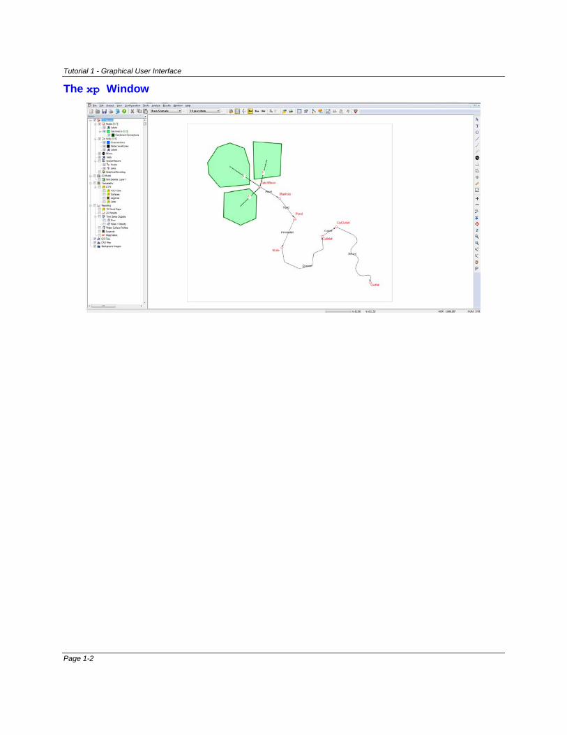
The xp Window
Page 1-2
Tutorial 1 - Graphical User Interface
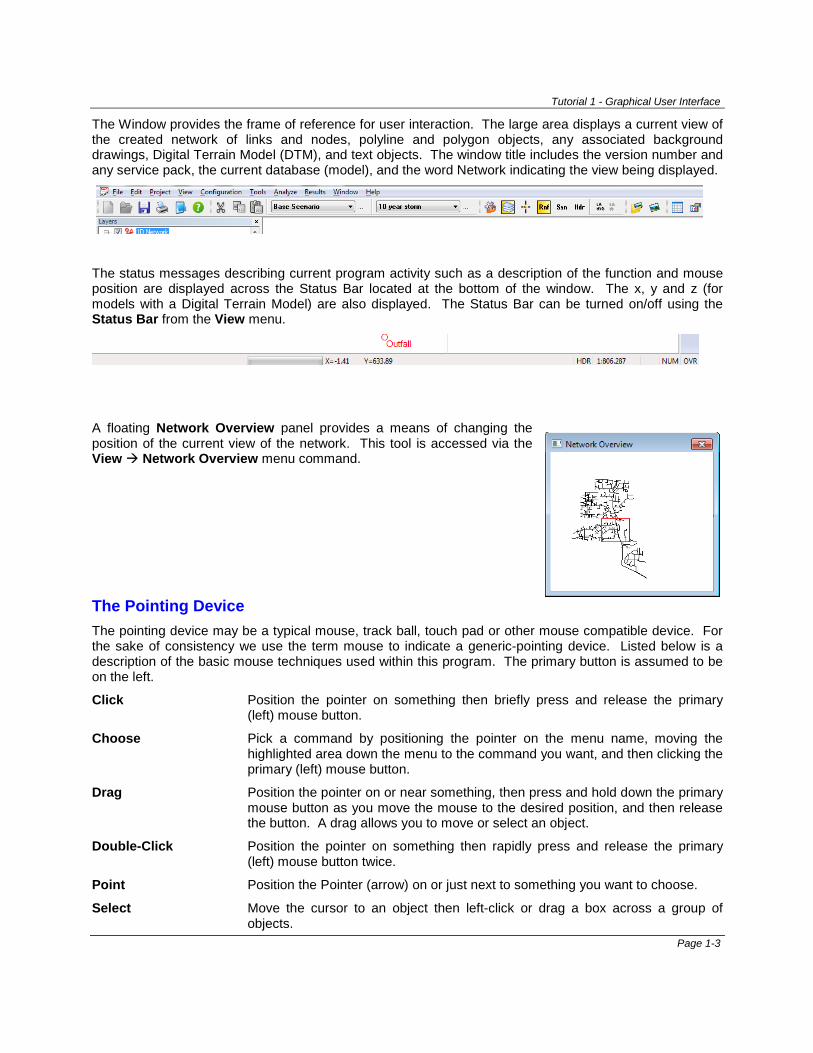
The Window provides the frame of reference for user interaction. The large area displays a current view of the created network of links and nodes, polyline and polygon objects, any associated background drawings, Digital Terrain Model (DTM), and text objects. The window title includes the version number and any service pack, the current database (model), and the word Network indicating the view being displayed.
The status messages describing current program activity such as a description of the function and mouse position are displayed across the Status Bar located at the bottom of the window. The x, y and z (for models with a Digital Terrain Model) are also displayed. The Status Bar can be turned on/off using the Status Bar from the View menu.
A floating Network Overview panel provides a means of changing the position of the current view of the network. This tool is accessed via the View Network Overview menu command.
The Pointing Device The pointing device may be a typical mouse, track ball, touch pad or other mouse compatible device. For the sake of consistency we use the term mouse to indicate a generic-pointing device. Listed below is a description of the basic mouse techniques used within this program. The primary button is assumed to be on the left.
Click Position the pointer on something then briefly press and release the primary (left) mouse button.
Choose Pick a command by positioning the pointer on the menu name, moving the highlighted area down the menu to the command you want, and then clicking the primary (left) mouse button.
Drag Position the pointer on or near something, then press and hold down the primary mouse button as you move the mouse to the desired position, and then release the button. A drag allows you to move or select an object.
Double-Click Position the pointer on something then rapidly press and release the primary (left) mouse button twice.
Point Position the Pointer (arrow) on or just next to something you want to choose.
Select Move the cursor to an object then left-click or drag a box across a group of objects.
Page 1-3
Tutorial 1 - Graphical User Interface
The mouse pointer changes shape to indicate the type of action that is taking place. The typical pointer icons are:
Pointer Icon You may select objects, move, re-connect or re-scale the network with this tool.
Text Icon Text annotation is being added to the network.
Node Icon Nodes are being added to the network.
Link Icon Single Links (solid line) are being added to the network.
Multi-Link Icon Multi-links (dashed line) are being added to the network.
Bridge Link Icon Bridge Links (segmented line) are being added to the network.
River Link Icon River Links (segmented lines and river nodes) are being added to the network.
Polyline icon A polyline is being drawn.
Polygon Icon A polygon is being created.
Trigger Point Icon Trigger Points are being added to the network.
Ruler Icon Lengths or areas are being measured from the network.
Section Profile Displays profile of selected cross section.
Catchment to Node The centroid of a catchment can be dragged to assign to a node catchment number.
Link Reattachment The head and tail of a link can be torn off and reattached to another node.
Blue Circle Icon The program is busy performing a task. The specific task is generally displayed in the status messages area of the window.
Hand Icon You are currently panning around the network.
Movable Icon An object will be displaced.
Semi-Circular Arrow A polygon grid will be rotated.
Define Cross Section Creates a cross section along selected points.
Edit Cross section Begin edit mode of selected cross section.
Insert Point Icon Add a vertex to a cross section, polylink, or polygon.
Move Point Icon Move a vertex of a cross section, polylink, or polygon.
The Mouse allows the user to select objects to operate on by pointing and clicking and similarly to initiate system commands through Pull-down menus and to select a tool.
Shortcut Keys Numerous keyboard shortcuts are available in xp. These are:
Ctrl-N Create a new project F1 Launch Help file Ctrl-A Add all nodes to selection F2 Open XP Tables Ctrl-L Add all links to selection F3 Conduit Profile for selected conduit Ctrl-C Copy F5 Solve the model Ctrl-V Paste Ctrl-F5 Snap Mode
Page 1-4
Tutorial 1 - Graphical User Interface
Ctrl-X Cut data F6 Browse file Ctrl-F Find, opens the Go To dialog F7 Review Results Ctrl-D Opens data dialog F8 Profile Plot Ctrl-R Redraws network view F9 Dynamic Long Section View Ctrl-O Open a file Shift-F9 Dynamic Section Views Ctrl-Q Exit xp application F10 Dynamic Plan View Ctrl-S Save the current xp file F11 Spatial Reports Ctrl-W Close xp file F12 Graphical Encoding Ctrl-P Print the current page DEL Delete selected objects and associated
data Ctrl-U Run Utilities Ctrl-M Display count of selected objects Ctrl-G Go to an X,Y coordinate
The Dialog Box
The Dialog Box is a graphical view of the attribute database. In other words the Dialog Box is to attribute data what the Window is to the network spatial data. The Dialog Box contains different types of items or controls that represent different types of data or modeling choices.
Three methods of accessing the node and link object dialogs are:
1. Double-click on the link or node or,
2. Left-click select the link or node, then right click for the menu then select edit data or,
3. Left-click to select the object and then from the menu select Edit Data (or Ctrl D).
The common items in the dialog box are described below:
Static Text Caption for Editable Text.
Editable Text Text strings or numbers. The insertion point for the text is contained in a rectangular field. Double-clicking in the field will select all text, and subsequent data entry will replace all existing text.
Check box A square check box is a flag for a particular option. You may select none, any or all options. A check box with underlying data is located on an action button. Check boxes are always optional.
Choice Button The circular choice buttons (Radio Buttons) indicate a choice of one item from a group of options. Only one option may be selected from the group. A choice button located on an action button indicates underlying data. The selection of one of the choice buttons is mandatory.
Action Button A rectangular action button controls dialog traversal (and therefore data structure). The OK and Cancel Action buttons are usually mapped to the <Enter> and <Esc> keys. The upper right hand corner X button on the dialog is also mapped to ESC and abandons all edits made in the dialog if pressed. A button item in a Job Control Dialog contains mandatory data. Other Action buttons include "Run" for the Utilities and "Import" for the Import dialog and “More” to load another dialog for complete data entry for a particular model section.
Picture A picture data item is an icon or a symbol used to promote rapid comprehension. It is not a dynamic item and is only representative of typical modeling scenarios.
Page 1-5
Tutorial 1 - Graphical User Interface
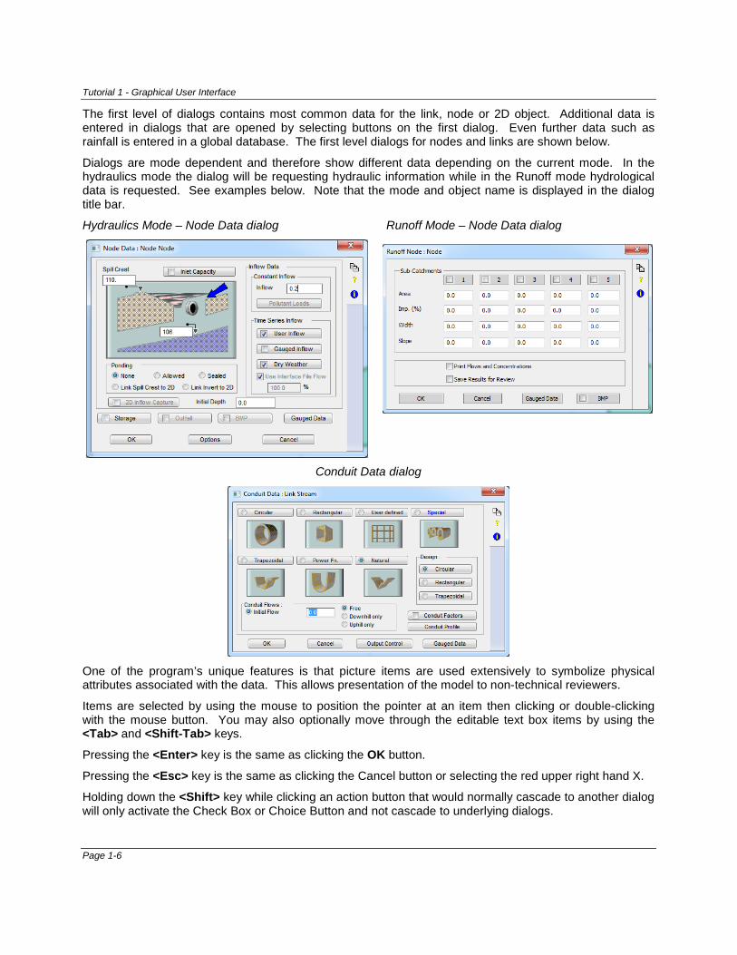
The first level of dialogs contains most common data for the link, node or 2D object. Additional data is entered in dialogs that are opened by selecting buttons on the first dialog. Even further data such as rainfall is entered in a global database. The first level dialogs for nodes and links are shown below.
Dialogs are mode dependent and therefore show different data depending on the current mode. In the hydraulics mode the dialog will be requesting hydraulic information while in the Runoff mode hydrological data is requested. See examples below. Note that the mode and object name is displayed in the dialog title bar.
Hydraulics Mode – Node Data dialog Runoff Mode – Node Data dialog
Conduit Data dialog
One of the program’s unique features is that picture items are used extensively to symbolize physical attributes associated with the data. This allows presentation of the model to non-technical reviewers.
Items are selected by using the mouse to position the pointer at an item then clicking or double-clicking with the mouse button. You may also optionally move through the editable text box items by using the <Tab> and <Shift-Tab> keys.
Pressing the <Enter> key is the same as clicking the OK button.
Pressing the <Esc> key is the same as clicking the Cancel button or selecting the red upper right hand X.
Holding down the <Shift> key while clicking an action button that would normally cascade to another dialog will only activate the Check Box or Choice Button and not cascade to underlying dialogs.
Page 1-6
Tutorial 1 - Graphical User Interface
Selecting the OK button causes an embedded expert system to check the data. If the data is not valid or it is unreasonable an error message or warning will be displayed respectively and you will have to return to the dialog. If the data is valid it is committed to the temporary database. The temporary database is written to the permanent database (your *.xp file) during a File Save or Save As command.
Selecting Cancel or the red X in the upper right hand corner will ignore any changes that have been made and will not invoke the data checking.
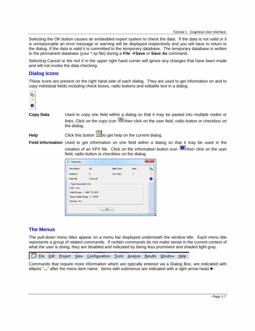
Dialog Icons These Icons are present on the right hand side of each dialog. They are used to get information on and to copy individual fields including check boxes, radio buttons and editable text in a dialog.
Copy Data Used to copy one field within a dialog so that it may be pasted into multiple nodes or
links. Click on the copy icon then click on the user field, radio button or checkbox on the dialog.
Help Click this button to get help on the current dialog.
Field Information Used to get information on one field within a dialog so that it may be used in the creation of an XPX file. Click on the information button icon then click on the user field, radio button or checkbox on the dialog.
The Menus The pull-down menu titles appear on a menu bar displayed underneath the window title. Each menu title represents a group of related commands. If certain commands do not make sense in the current context of what the user is doing, they are disabled and indicated by being less prominent and shaded light gray.
Commands that require more information which are typically entered via a Dialog Box, are indicated with ellipsis "..." after the menu item name. Items with submenus are indicated with a right arrow head ►.
Page 1-7
Tutorial 1 - Graphical User Interface
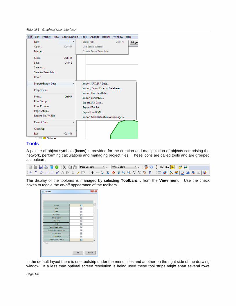
Tools A palette of object symbols (icons) is provided for the creation and manipulation of objects comprising the network, performing calculations and managing project files. These icons are called tools and are grouped as toolbars.
The display of the toolbars is managed by selecting Toolbars… from the View menu. Use the check boxes to toggle the on/off appearance of the toolbars.
In the default layout there is one toolstrip under the menu titles and another on the right side of the drawing window. If a less than optimal screen resolution is being used these tool strips might span several rows
Page 1-8
Tutorial 1 - Graphical User Interface
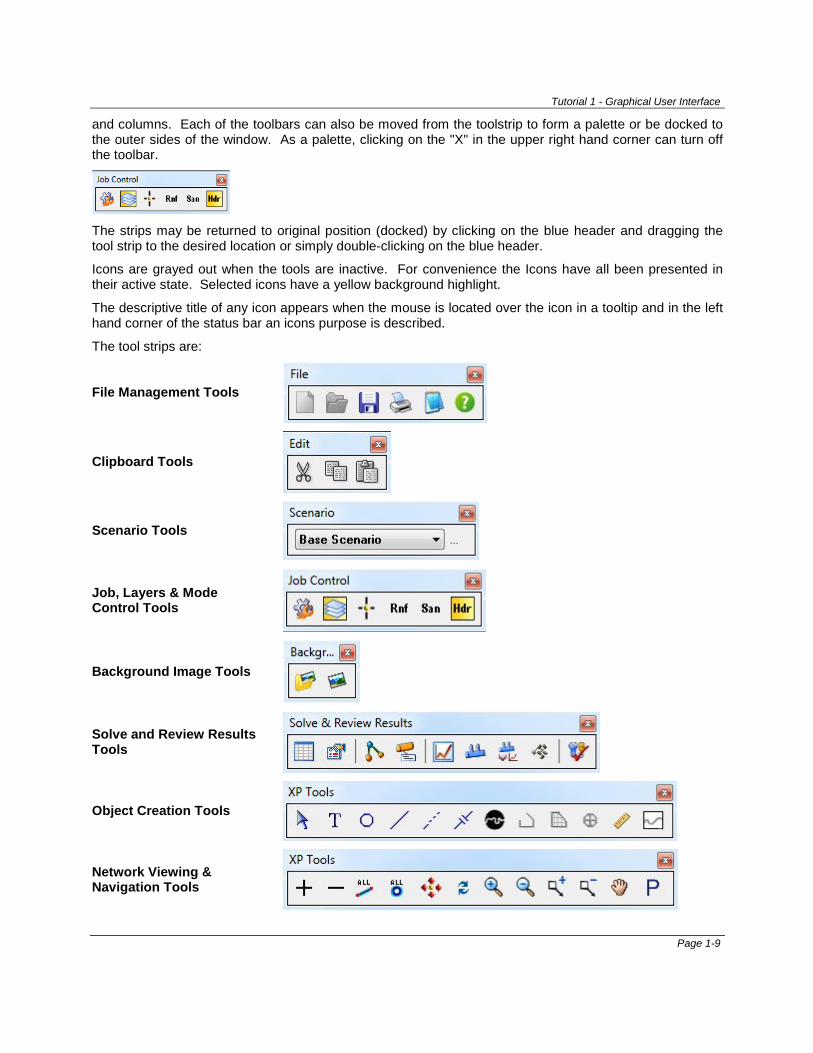
and columns. Each of the toolbars can also be moved from the toolstrip to form a palette or be docked to the outer sides of the window. As a palette, clicking on the "X" in the upper right hand corner can turn off the toolbar.
The strips may be returned to original position (docked) by clicking on the blue header and dragging the tool strip to the desired location or simply double-clicking on the blue header.
Icons are grayed out when the tools are inactive. For convenience the Icons have all been presented in their active state. Selected icons have a yellow background highlight.
The descriptive title of any icon appears when the mouse is located over the icon in a tooltip and in the left hand corner of the status bar an icons purpose is described.
The tool strips are:
File Management Tools
Clipboard Tools
Scenario Tools
Job, Layers & Mode Control Tools
Background Image Tools
Solve and Review Results Tools
Object Creation Tools
Network Viewing & Navigation Tools
Page 1-9
Tutorial 1 - Graphical User Interface
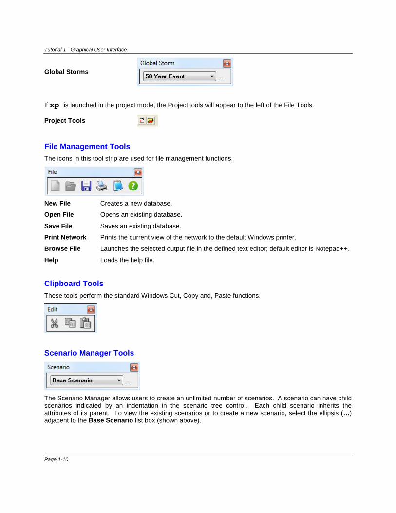
Global Storms
If xp is launched in the project mode, the Project tools will appear to the left of the File Tools.
Project Tools
File Management Tools The icons in this tool strip are used for file management functions.
New File Creates a new database.
Open File Opens an existing database.
Save File Saves an existing database.
Print Network Prints the current view of the network to the default Windows printer.
Browse File Launches the selected output file in the defined text editor; default editor is Notepad++.
Help Loads the help file.
Clipboard Tools These tools perform the standard Windows Cut, Copy and, Paste functions.
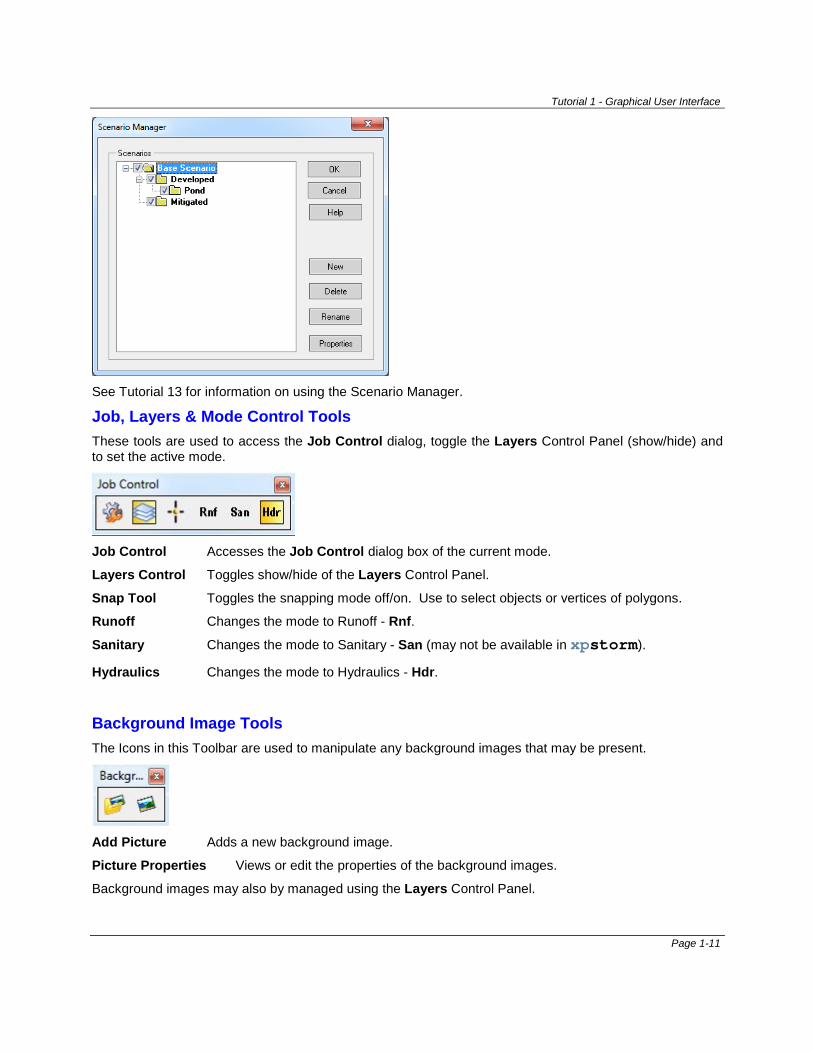
Scenario Manager Tools
The Scenario Manager allows users to create an unlimited number of scenarios. A scenario can have child scenarios indicated by an indentation in the scenario tree control. Each child scenario inherits the attributes of its parent. To view the existing scenarios or to create a new scenario, select the ellipsis (…) adjacent to the Base Scenario list box (shown above).
Page 1-10
Tutorial 1 - Graphical User Interface
See Tutorial 13 for information on using the Scenario Manager.
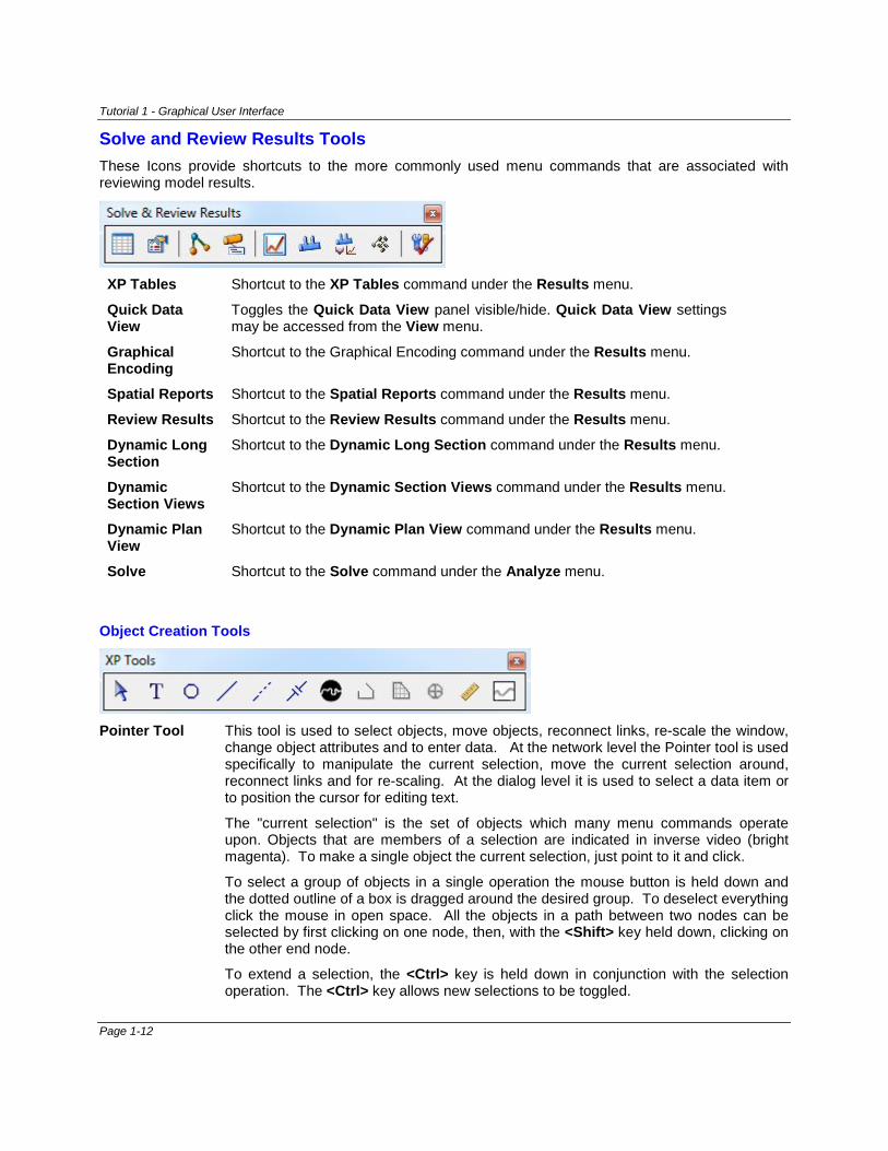
Job, Layers & Mode Control Tools These tools are used to access the Job Control dialog, toggle the Layers Control Panel (show/hide) and to set the active mode.
Job Control Accesses the Job Control dialog box of the current mode.
Layers Control Toggles show/hide of the Layers Control Panel.
Snap Tool Toggles the snapping mode off/on. Use to select objects or vertices of polygons.
Runoff Changes the mode to Runoff - Rnf.
Sanitary Changes the mode to Sanitary - San (may not be available in xpstorm).
Hydraulics Changes the mode to Hydraulics - Hdr.
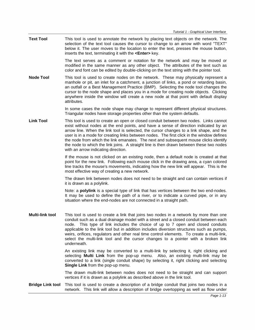
Background Image Tools The Icons in this Toolbar are used to manipulate any background images that may be present.
Add Picture Adds a new background image.
Picture Properties Views or edit the properties of the background images.
Background images may also by managed using the Layers Control Panel.
Page 1-11
Tutorial 1 - Graphical User Interface
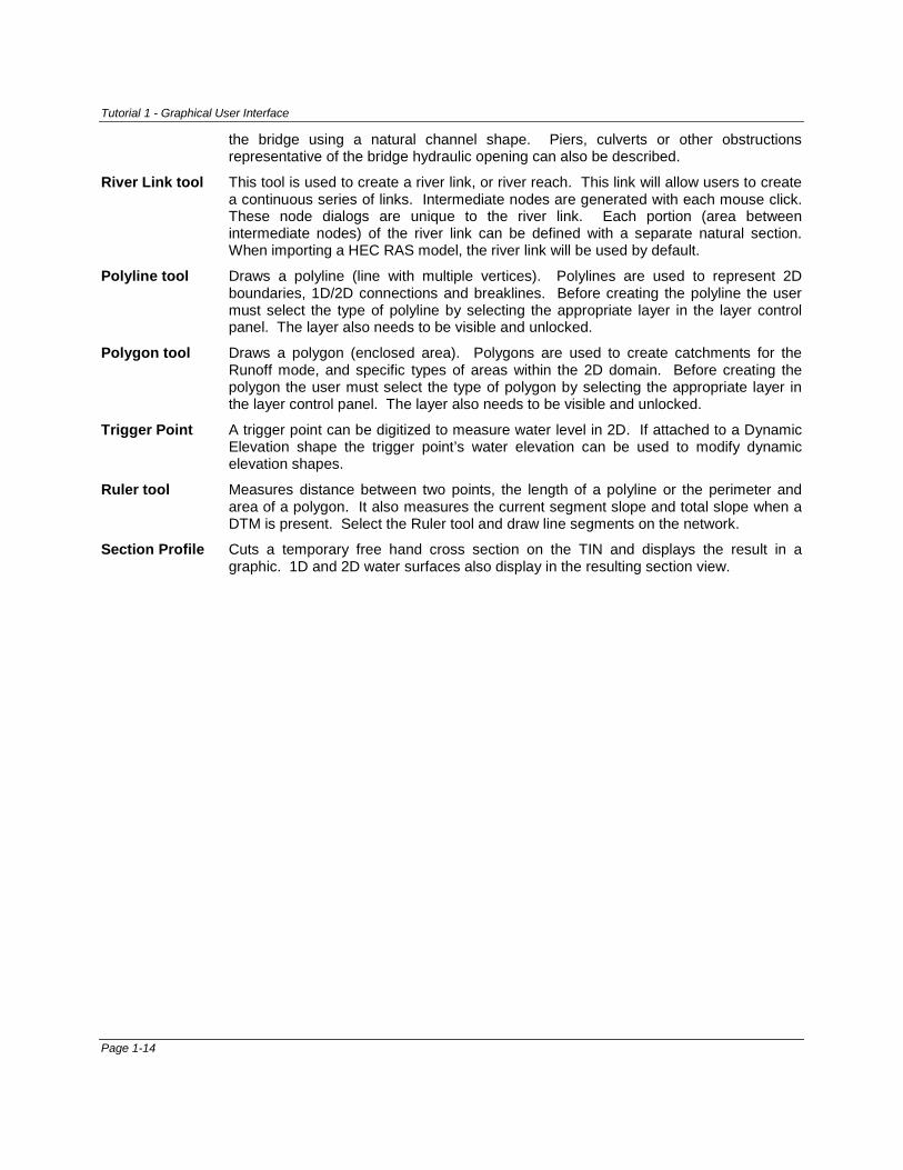
Solve and Review Results Tools These Icons provide shortcuts to the more commonly used menu commands that are associated with reviewing model results.
XP Tables Shortcut to the XP Tables command under the Results menu.
Quick Data View
Toggles the Quick Data View panel visible/hide. Quick Data View settings may be accessed from the View menu.
Graphical Encoding
Shortcut to the Graphical Encoding command under the Results menu.
Spatial Reports Shortcut to the Spatial Reports command under the Results menu.
Review Results Shortcut to the Review Results command under the Results menu.
Dynamic Long Section
Shortcut to the Dynamic Long Section command under the Results menu.
Dynamic Section Views
Shortcut to the Dynamic Section Views command under the Results menu.
Dynamic Plan View
Shortcut to the Dynamic Plan View command under the Results menu.
Solve Shortcut to the Solve command under the Analyze menu.
Object Creation Tools
Pointer Tool This tool is used to select objects, move objects, reconnect links, re-scale the window,
change object attributes and to enter data. At the network level the Pointer tool is used specifically to manipulate the current selection, move the current selection around, reconnect links and for re-scaling. At the dialog level it is used to select a data item or to position the cursor for editing text.
The "current selection" is the set of objects which many menu commands operate upon. Objects that are members of a selection are indicated in inverse video (bright magenta). To make a single object the current selection, just point to it and click.
To select a group of objects in a single operation the mouse button is held down and the dotted outline of a box is dragged around the desired group. To deselect everything click the mouse in open space. All the objects in a path between two nodes can be selected by first clicking on one node, then, with the <Shift> key held down, clicking on the other end node.
To extend a selection, the <Ctrl> key is held down in conjunction with the selection operation. The <Ctrl> key allows new selections to be toggled.
Page 1-12
Tutorial 1 - Graphical User Interface
Text Tool This tool is used to annotate the network by placing text objects on the network. The selection of the text tool causes the cursor to change to an arrow with word "TEXT" below it. The user moves to the location to enter the text, presses the mouse button, inserts the text, terminating it with the <Enter> key.
The text serves as a comment or notation for the network and may be moved or modified in the same manner as any other object. The attributes of the text such as color and font can be edited by double-clicking on the text string with the pointer tool.
Node Tool This tool is used to create nodes on the network. These may physically represent a manhole or pit, an inlet for a catchment, a junction of links, a pond or retarding basin, an outfall or a Best Management Practice (BMP). Selecting the node tool changes the cursor to the node shape and places you in a mode for creating node objects. Clicking anywhere inside the window will create a new node at that point with default display attributes.
In some cases the node shape may change to represent different physical structures. Triangular nodes have storage properties other than the system defaults.
Link Tool This tool is used to create an open or closed conduit between two nodes. Links cannot exist without nodes at the end points, and have a sense of direction indicated by an arrow line. When the link tool is selected, the cursor changes to a link shape, and the user is in a mode for creating links between nodes. The first click in the window defines the node from which the link emanates. The next and subsequent mouse clicks identify the node to which the link joins. A straight line is then drawn between these two nodes with an arrow indicating direction.
If the mouse is not clicked on an existing node, then a default node is created at that point for the new link. Following each mouse click in the drawing area, a cyan colored line tracks the mouse's movements, indicating how the new link will appear. This is the most effective way of creating a new network.
The drawn link between nodes does not need to be straight and can contain vertices if it is drawn as a polylink.
Note: a polylink is a special type of link that has vertices between the two end-nodes. It may be used to define the path of a river, or to indicate a curved pipe, or in any situation where the end-nodes are not connected in a straight path.
Multi-link tool This tool is used to create a link that joins two nodes in a network by more than one conduit such as a dual drainage model with a street and a closed conduit between each node. This type of link includes the choice of up to 7 open and closed conduits applicable to the link tool but in addition includes diversion structures such as pumps, weirs, orifices, regulators and other real time control elements. To create a multi-link, select the multi-link tool and the cursor changes to a pointer with a broken link underneath.
An existing link may be converted to a multi-link by selecting it, right clicking and selecting Multi Link from the pop-up menu. Also, an existing multi-link may be converted to a link (single conduit shape) by selecting it, right clicking and selecting Single Link from the pop-up menu.
The drawn multi-link between nodes does not need to be straight and can support vertices if it is drawn as a polylink as described above in the link tool.
Bridge Link tool This tool is used to create a description of a bridge conduit that joins two nodes in a network. This link will allow a description of bridge overtopping as well as flow under
Page 1-13
Tutorial 1 - Graphical User Interface
the bridge using a natural channel shape. Piers, culverts or other obstructions representative of the bridge hydraulic opening can also be described.
River Link tool This tool is used to create a river link, or river reach. This link will allow users to create a continuous series of links. Intermediate nodes are generated with each mouse click. These node dialogs are unique to the river link. Each portion (area between intermediate nodes) of the river link can be defined with a separate natural section. When importing a HEC RAS model, the river link will be used by default.
Polyline tool Draws a polyline (line with multiple vertices). Polylines are used to represent 2D boundaries, 1D/2D connections and breaklines. Before creating the polyline the user must select the type of polyline by selecting the appropriate layer in the layer control panel. The layer also needs to be visible and unlocked.
Polygon tool Draws a polygon (enclosed area). Polygons are used to create catchments for the Runoff mode, and specific types of areas within the 2D domain. Before creating the polygon the user must select the type of polygon by selecting the appropriate layer in the layer control panel. The layer also needs to be visible and unlocked.
Trigger Point A trigger point can be digitized to measure water level in 2D. If attached to a Dynamic Elevation shape the trigger point’s water elevation can be used to modify dynamic elevation shapes.
Ruler tool Measures distance between two points, the length of a polyline or the perimeter and area of a polygon. It also measures the current segment slope and total slope when a DTM is present. Select the Ruler tool and draw line segments on the network.
Section Profile Cuts a temporary free hand cross section on the TIN and displays the result in a graphic. 1D and 2D water surfaces also display in the resulting section view.
Page 1-14
Tutorial 1 - Graphical User Interface
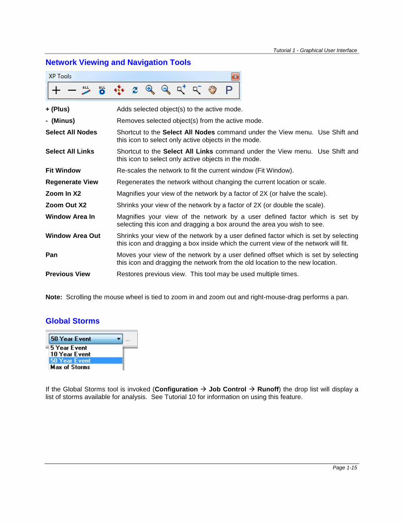
Network Viewing and Navigation Tools
+ (Plus) Adds selected object(s) to the active mode.
- (Minus) Removes selected object(s) from the active mode.
Select All Nodes Shortcut to the Select All Nodes command under the View menu. Use Shift and this icon to select only active objects in the mode.
Select All Links Shortcut to the Select All Links command under the View menu. Use Shift and this icon to select only active objects in the mode.
Fit Window Re-scales the network to fit the current window (Fit Window).
Regenerate View Regenerates the network without changing the current location or scale.
Zoom In X2 Magnifies your view of the network by a factor of 2X (or halve the scale).
Zoom Out X2 Shrinks your view of the network by a factor of 2X (or double the scale).
Window Area In Magnifies your view of the network by a user defined factor which is set by selecting this icon and dragging a box around the area you wish to see.
Window Area Out Shrinks your view of the network by a user defined factor which is set by selecting this icon and dragging a box inside which the current view of the network will fit.
Pan Moves your view of the network by a user defined offset which is set by selecting this icon and dragging the network from the old location to the new location.
Previous View Restores previous view. This tool may be used multiple times.
Note: Scrolling the mouse wheel is tied to zoom in and zoom out and right-mouse-drag performs a pan.
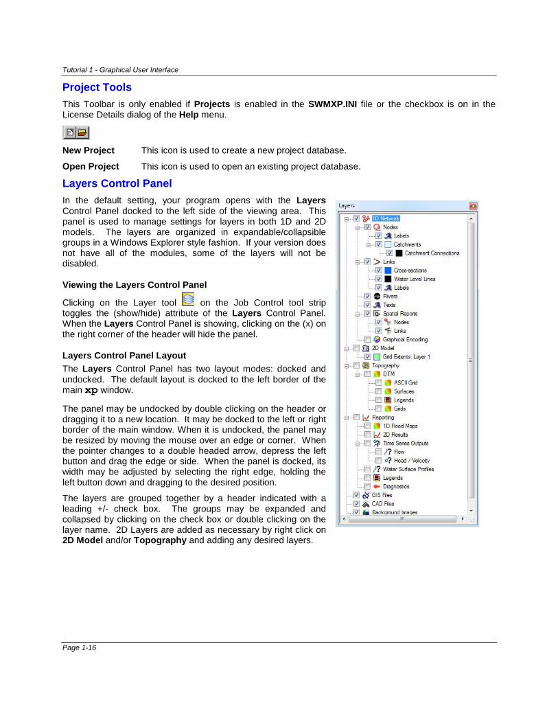
Global Storms
If the Global Storms tool is invoked (Configuration Job Control Runoff) the drop list will display a list of storms available for analysis. See Tutorial 10 for information on using this feature.
Page 1-15
Tutorial 1 - Graphical User Interface
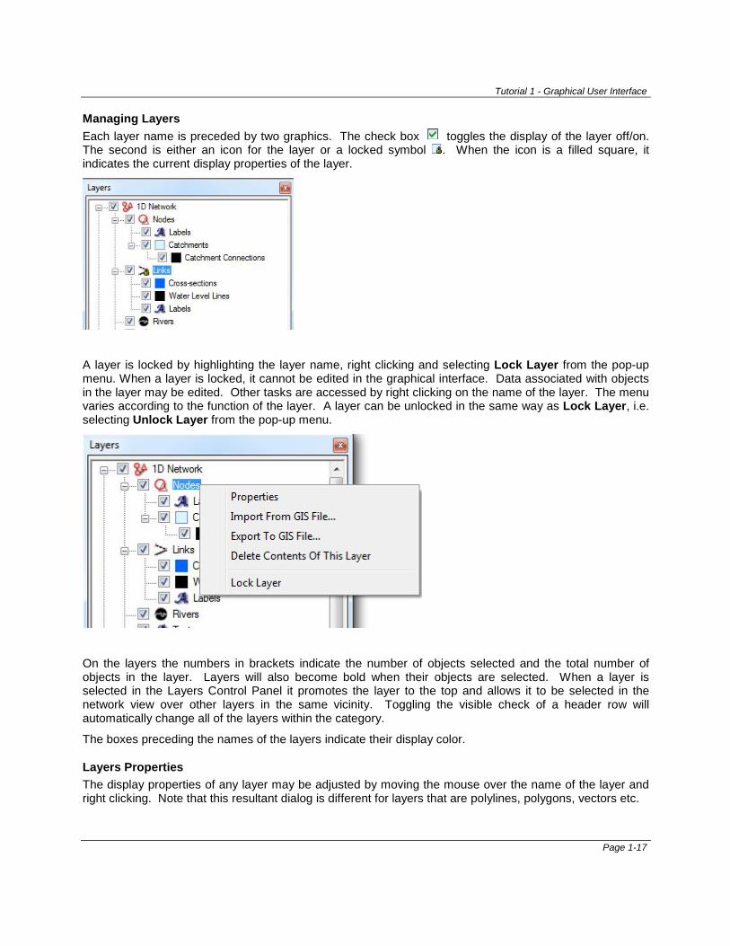
Project Tools This Toolbar is only enabled if Projects is enabled in the SWMXP.INI file or the checkbox is on in the License Details dialog of the Help menu.
New Project This icon is used to create a new project database.
Open Project This icon is used to open an existing project database.
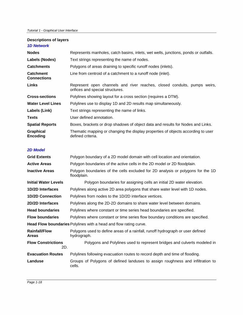
Layers Control Panel In the default setting, your program opens with the Layers Control Panel docked to the left side of the viewing area. This panel is used to manage settings for layers in both 1D and 2D models. The layers are organized in expandable/collapsible groups in a Windows Explorer style fashion. If your version does not have all of the modules, some of the layers will not be disabled.
Viewing the Layers Control Panel
Clicking on the Layer tool on the Job Control tool strip toggles the (show/hide) attribute of the Layers Control Panel. When the Layers Control Panel is showing, clicking on the (x) on the right corner of the header will hide the panel.
Layers Control Panel Layout The Layers Control Panel has two layout modes: docked and undocked. The default layout is docked to the left border of the main xp window.
The panel may be undocked by double clicking on the header or dragging it to a new location. It may be docked to the left or right border of the main window. When it is undocked, the panel may be resized by moving the mouse over an edge or corner. When the pointer changes to a double headed arrow, depress the left button and drag the edge or side. When the panel is docked, its width may be adjusted by selecting the right edge, holding the left button down and dragging to the desired position.
The layers are grouped together by a header indicated with a leading +/- check box. The groups may be expanded and collapsed by clicking on the check box or double clicking on the layer name. 2D Layers are added as necessary by right click on 2D Model and/or Topography and adding any desired layers.
Page 1-16
Tutorial 1 - Graphical User Interface
Managing Layers Each layer name is preceded by two graphics. The check box toggles the display of the layer off/on. The second is either an icon for the layer or a locked symbol . When the icon is a filled square, it indicates the current display properties of the layer.
A layer is locked by highlighting the layer name, right clicking and selecting Lock Layer from the pop-up menu. When a layer is locked, it cannot be edited in the graphical interface. Data associated with objects in the layer may be edited. Other tasks are accessed by right clicking on the name of the layer. The menu varies according to the function of the layer. A layer can be unlocked in the same way as Lock Layer, i.e. selecting Unlock Layer from the pop-up menu.
On the layers the numbers in brackets indicate the number of objects selected and the total number of objects in the layer. Layers will also become bold when their objects are selected. When a layer is selected in the Layers Control Panel it promotes the layer to the top and allows it to be selected in the network view over other layers in the same vicinity. Toggling the visible check of a header row will automatically change all of the layers within the category.
The boxes preceding the names of the layers indicate their display color.
Layers Properties The display properties of any layer may be adjusted by moving the mouse over the name of the layer and right clicking. Note that this resultant dialog is different for layers that are polylines, polygons, vectors etc.
Page 1-17
Tutorial 1 - Graphical User Interface
Descriptions of layers 1D Network
Nodes Represents manholes, catch basins, inlets, wet wells, junctions, ponds or outfalls.
Labels (Nodes) Text strings representing the name of nodes.
Catchments Polygons of areas draining to specific runoff nodes (inlets).
Catchment Line from centroid of a catchment to a runoff node (inlet). Connections
Links Represent open channels and river reaches, closed conduits, pumps weirs, orifices and special structures.
Cross-sections Polylines showing layout for a cross section (requires a DTM).
Water Level Lines Polylines use to display 1D and 2D results map simultaneously.
Labels (Link) Text strings representing the name of links.
Texts User defined annotation.
Spatial Reports Boxes, brackets or drop shadows of object data and results for Nodes and Links.
Graphical Thematic mapping or changing the display properties of objects according to user Encoding defined criteria.
2D Model
Grid Extents Polygon boundary of a 2D model domain with cell location and orientation.
Active Areas Polygon boundaries of the active cells in the 2D model or 2D floodplain.
Inactive Areas Polygon boundaries of the cells excluded for 2D analysis or polygons for the 1D floodplain.
Initial Water Levels Polygon boundaries for assigning cells an initial 2D water elevation.
1D/2D Interfaces Polylines along active 2D area polygons that share water level with 1D nodes.
1D/2D Connection Polylines from nodes to the 1D/2D interface vertices.
2D/2D Interfaces Polylines along the 2D-2D domains to share water level between domains.
Head boundaries Polylines where constant or time series head boundaries are specified.
Flow boundaries Polylines where constant or time series flow boundary conditions are specified.
Head Flow boundaries Polylines with a head and flow rating curve.
Rainfall/Flow Polygons used to define areas of a rainfall, runoff hydrograph or user defined Areas hydrograph.
Flow Constrictions Polygons and Polylines used to represent bridges and culverts modeled in 2D.
Evacuation Routes Polylines following evacuation routes to record depth and time of flooding.
Landuse Groups of Polygons of defined landuses to assign roughness and infiltration to cells.
Page 1-18
Tutorial 1 - Graphical User Interface
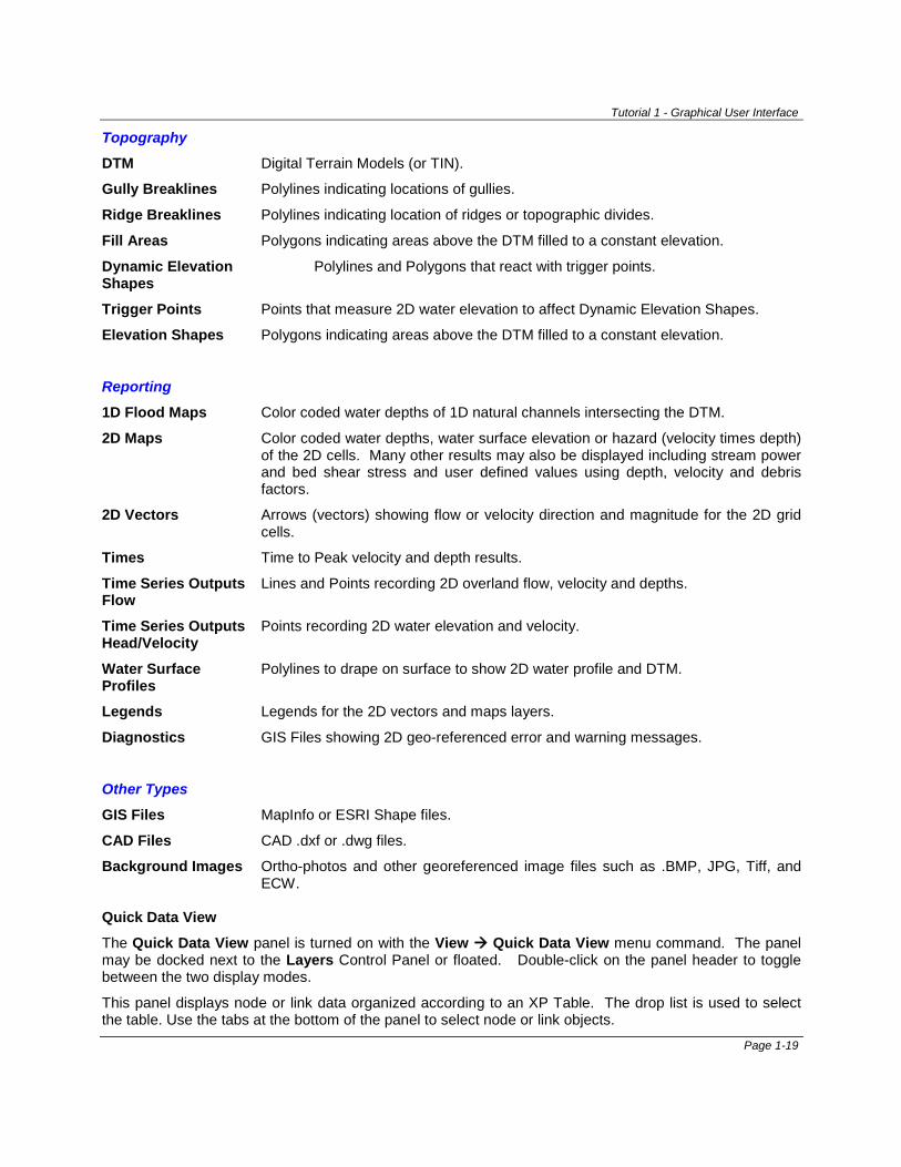
Topography
DTM Digital Terrain Models (or TIN).
Gully Breaklines Polylines indicating locations of gullies.
Ridge Breaklines Polylines indicating location of ridges or topographic divides.
Fill Areas Polygons indicating areas above the DTM filled to a constant elevation.
Dynamic Elevation Polylines and Polygons that react with trigger points. Shapes
Trigger Points Points that measure 2D water elevation to affect Dynamic Elevation Shapes.
Elevation Shapes Polygons indicating areas above the DTM filled to a constant elevation.
Reporting
1D Flood Maps Color coded water depths of 1D natural channels intersecting the DTM.
2D Maps Color coded water depths, water surface elevation or hazard (velocity times depth) of the 2D cells. Many other results may also be displayed including stream power and bed shear stress and user defined values using depth, velocity and debris factors.
2D Vectors Arrows (vectors) showing flow or velocity direction and magnitude for the 2D grid cells.
Times Time to Peak velocity and depth results.
Time Series Outputs Lines and Points recording 2D overland flow, velocity and depths. Flow
Time Series Outputs Points recording 2D water elevation and velocity. Head/Velocity
Water Surface Polylines to drape on surface to show 2D water profile and DTM. Profiles
Legends Legends for the 2D vectors and maps layers.
Diagnostics GIS Files showing 2D geo-referenced error and warning messages.
Other Types
GIS Files MapInfo or ESRI Shape files.
CAD Files CAD .dxf or .dwg files.
Background Images Ortho-photos and other georeferenced image files such as .BMP, JPG, Tiff, and ECW.
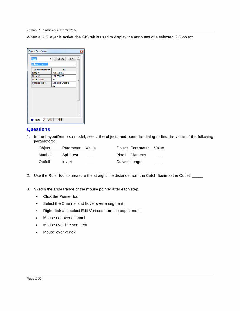
Quick Data View
The Quick Data View panel is turned on with the View Quick Data View menu command. The panel may be docked next to the Layers Control Panel or floated. Double-click on the panel header to toggle between the two display modes.
This panel displays node or link data organized according to an XP Table. The drop list is used to select the table. Use the tabs at the bottom of the panel to select node or link objects.
Page 1-19
Tutorial 1 - Graphical User Interface
When a GIS layer is active, the GIS tab is used to display the attributes of a selected GIS object.
Questions 1. In the LayoutDemo.xp model, select the objects and open the dialog to find the value of the following
parameters:
Object Parameter Value Object Parameter Value
Manhole Spillcrest ____ Pipe1 Diameter ____
Outfall Invert ____ Culvert Length ____
2. Use the Ruler tool to measure the straight line distance from the Catch Basin to the Outlet. _____
3. Sketch the appearance of the mouse pointer after each step.
• Click the Pointer tool
• Select the Channel and hover over a segment
• Right click and select Edit Vertices from the popup menu
• Mouse not over channel
• Mouse over line segment
• Mouse over vertex
Page 1-20
Surface Water Hydrology In Runoff mode (Rnf), the program simulates the rainfall, infiltration, evaporation, and depression storage, for each subcatchment, and calculates the runoff to a collection node. A variety of hydrologic methods is available to generate runoff hydrographs. In this tutorial, users will learn how to utilize XP’s tools to layout a collection system network and develop input data from GIS files. Standard design storms will be imported from a template file. Runoff will be simulated using both SCS and EPA SWMM hydrology. Finally, model results will be reviewed graphically and in tabular format. Users are advised to review The XP User Interface tutorial for an overview of the windows, menus, tools and basic concepts of building and navigating a stormwater collection network with XP’s graphical interface.
Part 1 – Laying out a network using GIS layers A collection network can be developed in the graphical interface using a variety of methods. In Part 1, users will learn how to utilize XP tools to layout a collection system network over GIS background images and to develop input data from information in GIS files.
Level: Beginner
Objectives: Introduce the steps required to: • Layout a runoff collection network using a background image for node locations • Define subcatchment drainage areas using a DTM layer • Use XP tools to calculate subcatchment areas • Connect subcatchments to runoff nodes
Time: 1 hour
Model Capability Number of Links/Nodes: 9/10 Add-on Modules: none 2D Size : none Requirement Evaluation Version Compatible: Yes
Data files: Contours.xyz (used to create TIN) Yarra_Area.dwg (background image)
1. Launch the program. At the opening dialog, select New. In the Windows Explorer, navigate to the
desired folder and name the file Yarra21. A file with the default extension (.xp) will be created.
In the Units dialog, select US Customary and click on OK.
2. Add the CAD layer. On the Layers Control Panel, check the visible box for CAD Files. Highlight the CAD Files layer and right click. From the popup menu, select Load CAD File.
In the dialog select the file Yarra_Area.dwg. Click on Open to display the image on the network view. This file is georeferenced so that its x and y coordinates are coincident with the proposed drainage network.
XP Solutions Tutorial 2 - Surface Water Hydrology
Tutorial 2 - Surface Water Hydrology
3. Browse the project site. Hold the mouse wheel or right button down and the moving hand (Pan
Tool) appears next to the cursor. Drag the screen around. Roll the wheel forward to zoom in and backwards to zoom out.
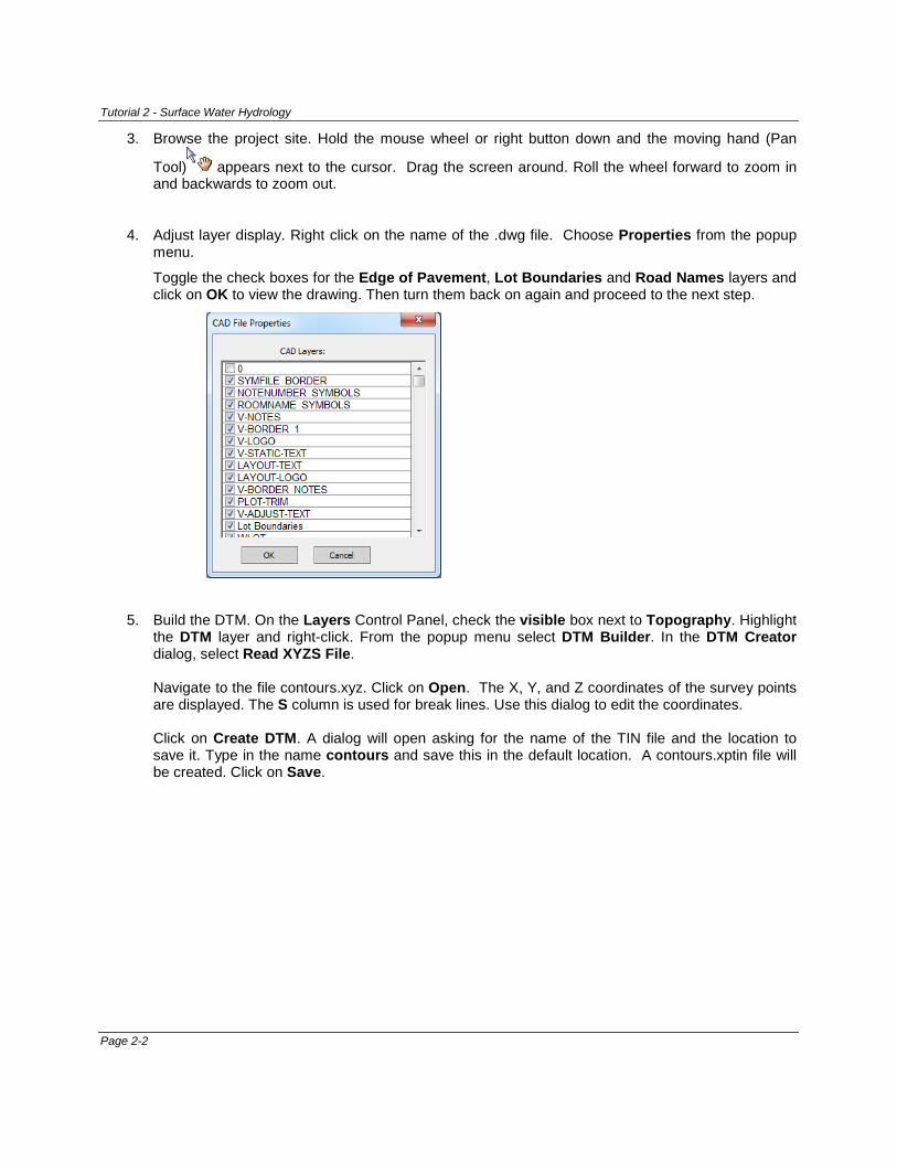
4. Adjust layer display. Right click on the name of the .dwg file. Choose Properties from the popup menu.
Toggle the check boxes for the Edge of Pavement, Lot Boundaries and Road Names layers and click on OK to view the drawing. Then turn them back on again and proceed to the next step.
5. Build the DTM. On the Layers Control Panel, check the visible box next to Topography. Highlight
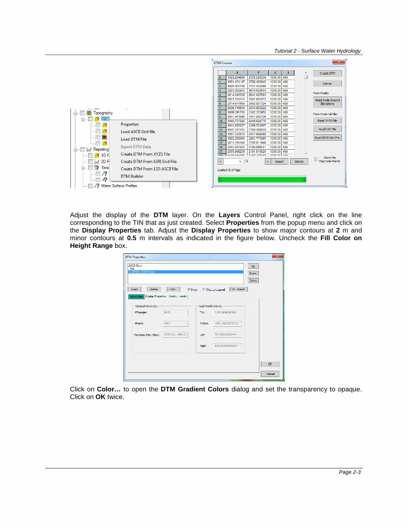
the DTM layer and right-click. From the popup menu select DTM Builder. In the DTM Creator dialog, select Read XYZS File. Navigate to the file contours.xyz. Click on Open. The X, Y, and Z coordinates of the survey points are displayed. The S column is used for break lines. Use this dialog to edit the coordinates. Click on Create DTM. A dialog will open asking for the name of the TIN file and the location to save it. Type in the name contours and save this in the default location. A contours.xptin file will be created. Click on Save.
Page 2-2
Tutorial 2 - Surface Water Hydrology
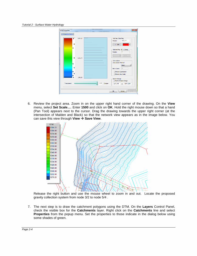
Adjust the display of the DTM layer. On the Layers Control Panel, right click on the line corresponding to the TIN that as just created. Select Properties from the popup menu and click on the Display Properties tab. Adjust the Display Properties to show major contours at 2 m and minor contours at 0.5 m intervals as indicated in the figure below. Uncheck the Fill Color on Height Range box.
Click on Color… to open the DTM Gradient Colors dialog and set the transparency to opaque. Click on OK twice.
Page 2-3
Tutorial 2 - Surface Water Hydrology
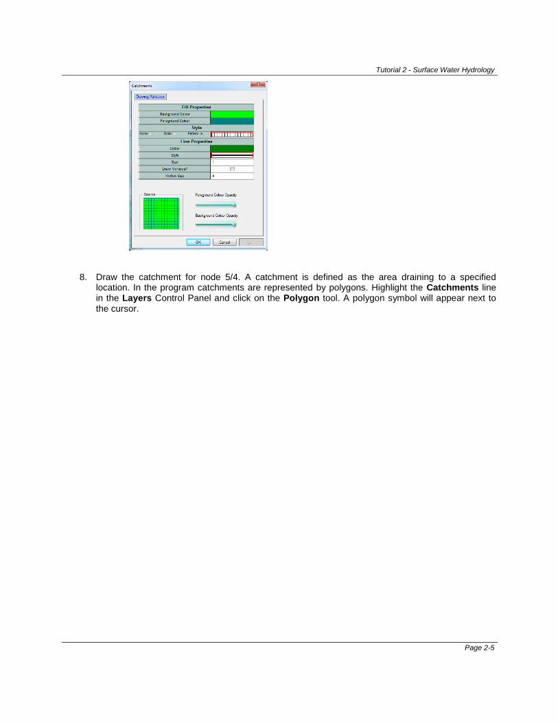
6. Review the project area. Zoom in on the upper right hand corner of the drawing. On the View menu, select Set Scale…. Enter 1500 and click on OK. Hold the right mouse down so that a hand (Pan Tool) appears next to the cursor. Drag the drawing towards the upper right corner (at the intersection of Malden and Black) so that the network view appears as in the image below. You can save this view through View Save View.
Release the right button and use the mouse wheel to zoom in and out. Locate the proposed gravity collection system from node 3/2 to node 5/4 .
7. The next step is to draw the catchment polygons using the DTM. On the Layers Control Panel,
check the visible box for the Catchments layer. Right click on the Catchments line and select Properties from the popup menu. Set the properties to those indicate in the dialog below using some shades of green.
Page 2-4
Tutorial 2 - Surface Water Hydrology
8. Draw the catchment for node 5/4. A catchment is defined as the area draining to a specified
location. In the program catchments are represented by polygons. Highlight the Catchments line in the Layers Control Panel and click on the Polygon tool. A polygon symbol will appear next to the cursor.
Page 2-5
Tutorial 2 - Surface Water Hydrology
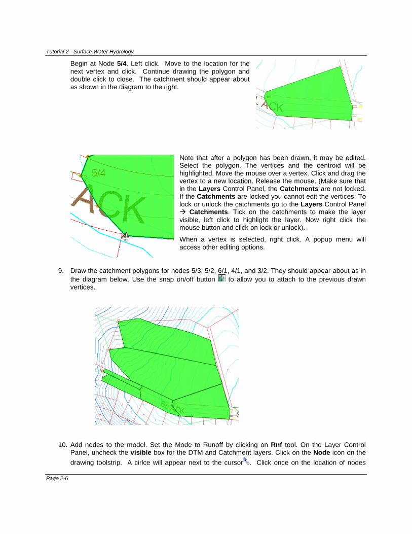
Begin at Node 5/4. Left click. Move to the location for the next vertex and click. Continue drawing the polygon and double click to close. The catchment should appear about as shown in the diagram to the right.
Note that after a polygon has been drawn, it may be edited. Select the polygon. The vertices and the centroid will be highlighted. Move the mouse over a vertex. Click and drag the vertex to a new location. Release the mouse. (Make sure that in the Layers Control Panel, the Catchments are not locked. If the Catchments are locked you cannot edit the vertices. To lock or unlock the catchments go to the Layers Control Panel Catchments. Tick on the catchments to make the layer visible, left click to highlight the layer. Now right click the mouse button and click on lock or unlock).
When a vertex is selected, right click. A popup menu will access other editing options.
9. Draw the catchment polygons for nodes 5/3, 5/2, 6/1, 4/1, and 3/2. They should appear about as in the diagram below. Use the snap on/off button to allow you to attach to the previous drawn vertices.
10. Add nodes to the model. Set the Mode to Runoff by clicking on Rnf tool. On the Layer Control Panel, uncheck the visible box for the DTM and Catchment layers. Click on the Node icon on the drawing toolstrip. A cirlce will appear next to the cursor . Click once on the location of nodes
Page 2-6
Tutorial 2 - Surface Water Hydrology
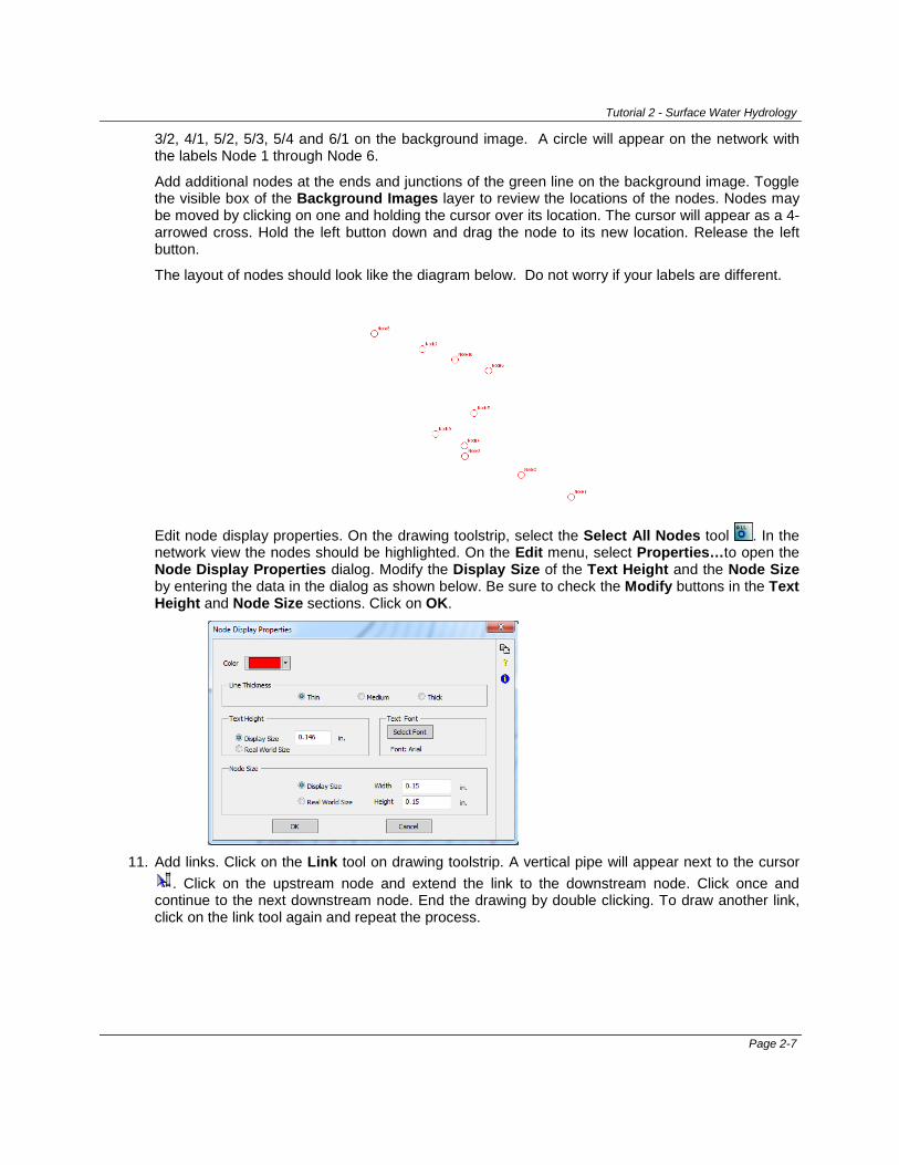
3/2, 4/1, 5/2, 5/3, 5/4 and 6/1 on the background image. A circle will appear on the network with the labels Node 1 through Node 6.
Add additional nodes at the ends and junctions of the green line on the background image. Toggle the visible box of the Background Images layer to review the locations of the nodes. Nodes may be moved by clicking on one and holding the cursor over its location. The cursor will appear as a 4-arrowed cross. Hold the left button down and drag the node to its new location. Release the left button.
The layout of nodes should look like the diagram below. Do not worry if your labels are different.
Edit node display properties. On the drawing toolstrip, select the Select All Nodes tool . In the network view the nodes should be highlighted. On the Edit menu, select Properties…to open the Node Display Properties dialog. Modify the Display Size of the Text Height and the Node Size by entering the data in the dialog as shown below. Be sure to check the Modify buttons in the Text Height and Node Size sections. Click on OK.
11. Add links. Click on the Link tool on drawing toolstrip. A vertical pipe will appear next to the cursor
. Click on the upstream node and extend the link to the downstream node. Click once and continue to the next downstream node. End the drawing by double clicking. To draw another link, click on the link tool again and repeat the process.
Page 2-7
Tutorial 2 - Surface Water Hydrology
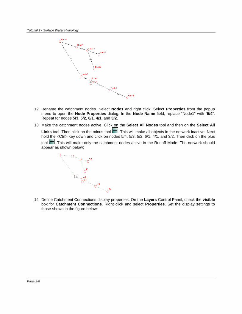
12. Rename the catchment nodes. Select Node1 and right click. Select Properties from the popup
menu to open the Node Properties dialog. In the Node Name field, replace “Node1” with “5/4”. Repeat for nodes 5/3, 5/2, 6/1, 4/1, and 3/2.
13. Make the catchment nodes active. Click on the Select All Nodes tool and then on the Select All Links tool. Then click on the minus tool . This will make all objects in the network inactive. Next hold the <Ctrl> key down and click on nodes 5/4, 5/3, 5/2, 6/1, 4/1, and 3/2. Then click on the plus tool . This will make only the catchment nodes active in the Runoff Mode. The network should appear as shown below:
14. Define Catchment Connections display properties. On the Layers Control Panel, check the visible
box for Catchment Connections. Right click and select Properties. Set the display settings to those shown in the figure below:
Page 2-8
Tutorial 2 - Surface Water Hydrology
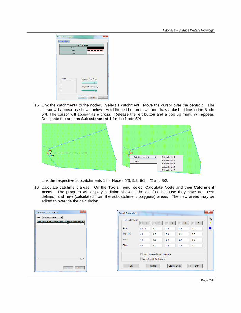
15. Link the catchments to the nodes. Select a catchment. Move the cursor over the centroid. The
cursor will appear as shown below. Hold the left button down and draw a dashed line to the Node 5/4. The cursor will appear as a cross. Release the left button and a pop up menu will appear. Designate the area as Subcatchment 1 for the Node 5/4
Link the respective subcatchments 1 for Nodes 5/3, 5/2, 6/1, 4/2 and 3/2.
16. Calculate catchment areas. On the Tools menu, select Calculate Node and then Catchment Areas. The program will display a dialog showing the old (0.0 because they have not been defined) and new (calculated from the subcatchment polygons) areas. The new areas may be edited to override the calculation.
Page 2-9

Tutorial 2 - Surface Water Hydrology
Click on OK to accept the new values. This data is added to the model database. This function will report that the calculation was successfully completed. Review the data for node 5/4 by double clicking on it.
17. Save your file as Yarra21.xp.
Questions
1. In regards to the DTM used in this exercise, what are the:
Number of suvery points _____
Minimum elevation _____ ft
Maximum elevation _____ ft
2. Open the File menu, select Properties and click on Job Statistics. In the current column what are the number of:
_____ links
_____ nodes
_____ pictures
3. Program allows up to _____ subcatchments per runoff collection node.
Page 2-10
Tutorial 2 - Surface Water Hydrology
Part 2 – Adding Design Storms and SCS Hydrology
In the program design storms and rainfall hyetographs can be imported by a variety of methods. In the United States and elsewhere, a set of commonly used design storms are the SCS 24-hour cumulative storms. This section demonstrates how a SCS rainfall distribution is imported using XPX formated files and developed into a design storm.
Level: Beginner
Objectives: Introduce the steps required to: • Import global storms from XPX files • Assign design storms to subcatchments
Time: 0.5 hours
Data files: Yarra21.xp (model developed in Part 1) Yarra_Area.dwg contours.xptin (DTM developed in Part 1)
SCS Rainfall Distributions 1inch(mm).xpx (design storm hyetographs)
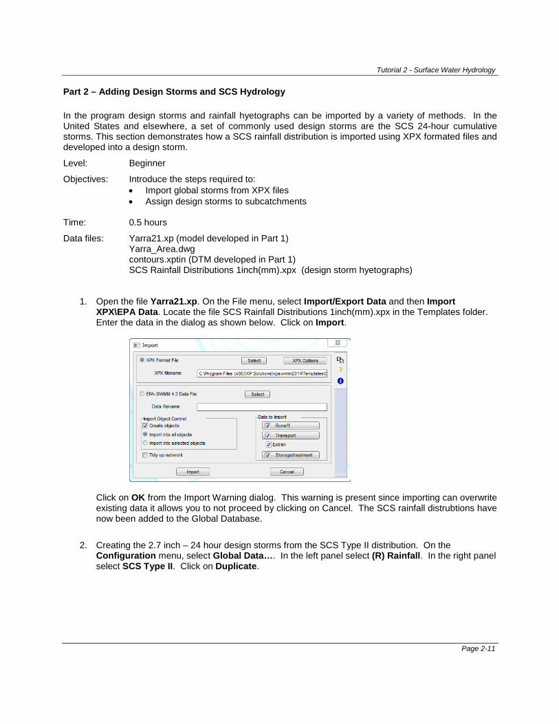
1. Open the file Yarra21.xp. On the File menu, select Import/Export Data and then Import
XPX\EPA Data. Locate the file SCS Rainfall Distributions 1inch(mm).xpx in the Templates folder. Enter the data in the dialog as shown below. Click on Import.
Click on OK from the Import Warning dialog. This warning is present since importing can overwrite existing data it allows you to not proceed by clicking on Cancel. The SCS rainfall distrubtions have now been added to the Global Database.
2. Creating the 2.7 inch – 24 hour design storms from the SCS Type II distribution. On the
Configuration menu, select Global Data…. In the left panel select (R) Rainfall. In the right panel select SCS Type II. Click on Duplicate.
Page 2-11
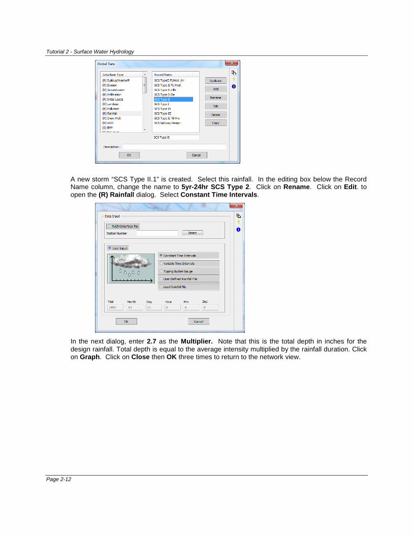
Tutorial 2 - Surface Water Hydrology
A new storm “SCS Type II.1” is created. Select this rainfall. In the editing box below the Record Name column, change the name to 5yr-24hr SCS Type 2. Click on Rename. Click on Edit. to open the (R) Rainfall dialog. Select Constant Time Intervals.
In the next dialog, enter 2.7 as the Multiplier. Note that this is the total depth in inches for the design rainfall. Total depth is equal to the average intensity multiplied by the rainfall duration. Click on Graph. Click on Close then OK three times to return to the network view.
Page 2-12

Tutorial 2 - Surface Water Hydrology
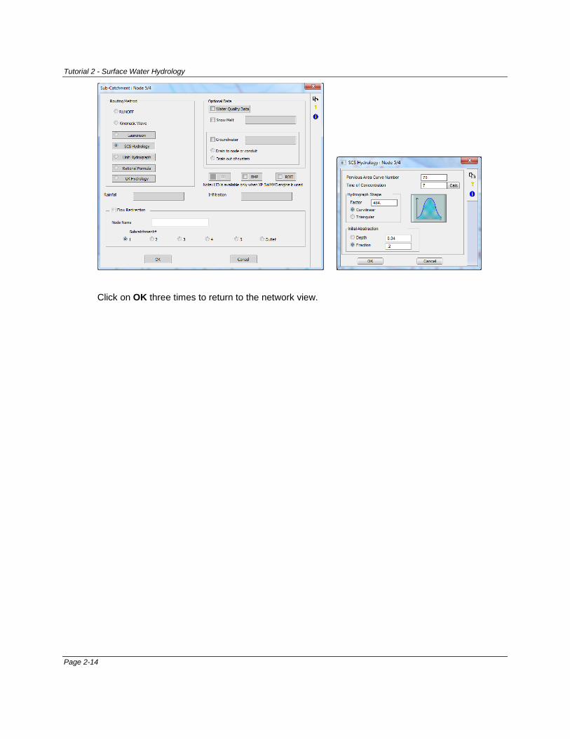
3. Enter the SCS Hydrology data. Make sure that the mode is set to Rnf (Runoff Mode). Double-click on Node 5/4 to open the runoff dialog. In this model only subcatchment 1 is used for each node. The area has been previously calculated. The Width and Slope are not used in SCS Hydrology. However, the program requires that these fields have nonzero values – enter 1 for each. Click on the 1 button to activate the subcatchment and advance to the next dialog. Set the Impervious Percent (Imp %) to 20.
4.
Click on the Rainfall button. Select the 5yr-24hr SCS Type 2 storm from the Global Database. Click on the SCS Hydrology button. In the SCS Hydrology dialog, set the Pervious Area Curve Number to 70 and the Time of Concentration to 7 minutes. Use the remaining default values.
Page 2-13
Tutorial 2 - Surface Water Hydrology
Click on OK three times to return to the network view.
Page 2-14

Tutorial 2 - Surface Water Hydrology
In a similar manner enter the following data for the remaining runoff nodes.
Node Imp. (%) Pervious Area Curve Number
Time of Concentration (min)
5/3 60 70 5
5/2 40 70 5
6/1 45 70 5
4/1 20 70 10
3/2 30 70 8
5. Save your file as Yarra22.xp.
Questions
1. In regards to the 5yr-24 SCS Type 2 storm used in this exercise, what is the:
Total rainfall _____ in.
Maximum intensity _____ in/hr
Time of Maximum intensity _____
2. Does the program require the rainfall to be the same over the entire network?
Page 2-15
Tutorial 2 - Surface Water Hydrology
Part 3 – Job Control Settings & Running the Model In the program settings for the calculation are managed in the Job Control dialog. This part reviews some of the Job Control settings in Runoff mode.
Level: Beginner
Objectives: Introduce the steps required to: • Manage runoff job control settings • Run the analysis
Time: 0.5 hours
Data files: Yarra22.xp (model developed in Part 2) Yarra_Area.dwg contours.xptin (DTM developed in Part 1)
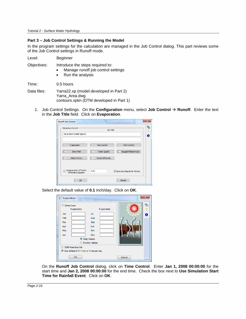
1. Job Control Settings. On the Configuration menu, select Job Control Runoff. Enter the text
in the Job Title field. Click on Evaporation.
Select the default value of 0.1 inch/day. Click on OK.
On the Runoff Job Control dialog, click on Time Control. Enter Jan 1, 2008 00:00:00 for the start time and Jan 2, 2008 00:00:00 for the end time. Check the box next to Use Simulation Start Time for Rainfall Event. Click on OK.
Page 2-16
Tutorial 2 - Surface Water Hydrology
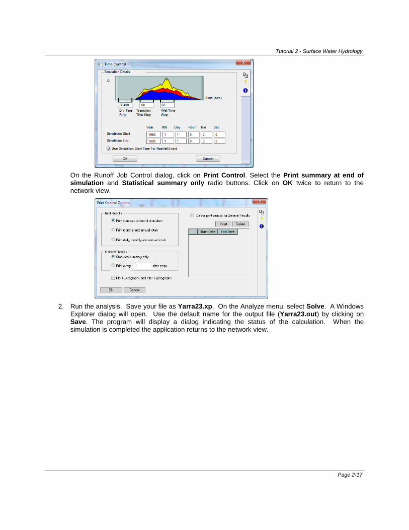
On the Runoff Job Control dialog, click on Print Control. Select the Print summary at end of simulation and Statistical summary only radio buttons. Click on OK twice to return to the network view.
2. Run the analysis. Save your file as Yarra23.xp. On the Analyze menu, select Solve. A Windows
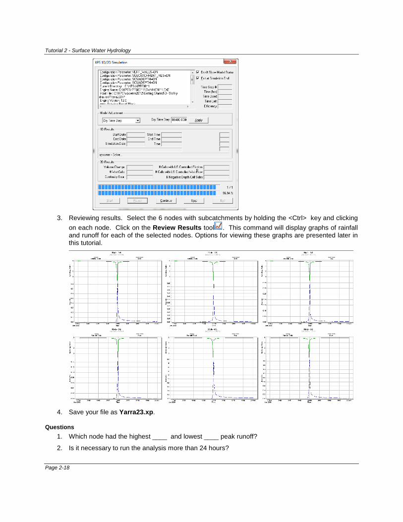
Explorer dialog will open. Use the default name for the output file (Yarra23.out) by clicking on Save. The program will display a dialog indicating the status of the calculation. When the simulation is completed the application returns to the network view.
Page 2-17
Tutorial 2 - Surface Water Hydrology
3. Reviewing results. Select the 6 nodes with subcatchments by holding the <Ctrl> key and clicking
on each node. Click on the Review Results tool . This command will display graphs of rainfall and runoff for each of the selected nodes. Options for viewing these graphs are presented later in this tutorial.
4. Save your file as Yarra23.xp.
Questions 1. Which node had the highest ____ and lowest ____ peak runoff?
2. Is it necessary to run the analysis more than 24 hours?
Page 2-18
Tutorial 2 - Surface Water Hydrology
Part 4 – SWMM Hydrology (Non-Linear Reservoir Method) Another popular catchment routing procedure is the EPA SWMM non-linear “Runoff” method. Overland flow hydrographs are generated by a routing procedure using Manning’s equation and a lumped continuity equation. Surface roughness and depression storage for pervious and impervious area parameters further describe the catchment. The subcatchment width parameter is related to the collection length of overland flow and is easily calculated based on the watershed area. The method can include infiltration modeled with the Horton or Green-Ampt equations or using a uniform loss rate.
Level: Beginner
Objectives: Introduce the steps required to: • Define the runoff parameters in a subcatchment • Use graphical interface tools to develop subcatchment data • Use the global database to manage infiltration data • Use graphical tools to obtain data from catchment parameters
Time: 0.5 hours
Data files: Yarra23.xp (same as file developed in Part 3) Yarra_Area.dwg contours.xptin (DTM developed in Part 1)
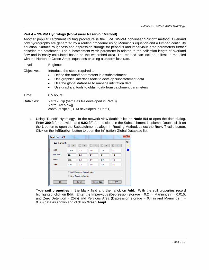
1. Using “Runoff” Hydrology. In the network view double click on Node 5/4 to open the data dialog. Enter 300 ft for the width and 0.02 ft/ft for the slope in the Subcatchment 1 column. Double click on the 1 button to open the Subcatchment dialog. In Routing Method, select the Runoff radio button. Click on the Infiltration button to open the Infiltration Global Database list.
Type soil properties in the blank field and then click on Add. With the soil properties record highlighted, click on Edit. Enter the Impervious (Depression storage = 0.2 in, Mannings n = 0.015, and Zero Detention = 25%) and Pervious Area (Depression storage = 0.4 in and Mannings n = 0.05) data as shown and click on Green Ampt.
Page 2-19
Tutorial 2 - Surface Water Hydrology
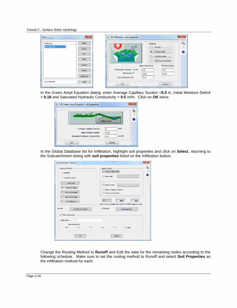
In the Green Ampt Equation dialog, enter Average Capillary Suction =5.0 in, Initial Moisture Deficit = 0.18 and Saturated Hydraulic Conductivity = 0.5 in/hr. Click on OK twice.
In the Global Database list for Infiltration, highlight soil properties and click on Select, returning to the Subcatchment dialog with soil properties listed on the Infiltration button.
Change the Routing Method to Runoff and Edit the data for the remaining nodes according to the following schedule. Make sure to set the routing method to Runoff and select Soil Properties as the infiltration method for each.
Page 2-20
Tutorial 2 - Surface Water Hydrology
Node Width, ft Slope, ft/ft
5/3 350 0.01
5/2 200 0.05
6/1 225 0.05
4/1 150 0.02
3/2 135 0.03
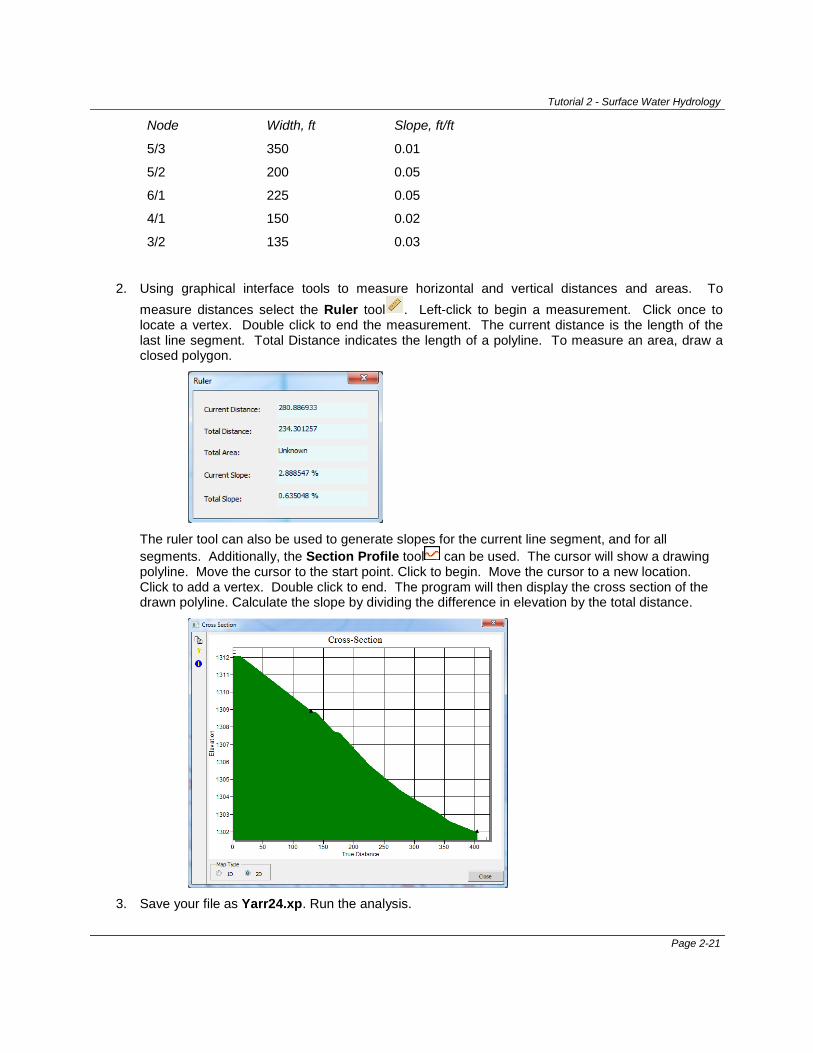
2. Using graphical interface tools to measure horizontal and vertical distances and areas. To measure distances select the Ruler tool . Left-click to begin a measurement. Click once to locate a vertex. Double click to end the measurement. The current distance is the length of the last line segment. Total Distance indicates the length of a polyline. To measure an area, draw a closed polygon.
The ruler tool can also be used to generate slopes for the current line segment, and for all segments. Additionally, the Section Profile tool can be used. The cursor will show a drawing polyline. Move the cursor to the start point. Click to begin. Move the cursor to a new location. Click to add a vertex. Double click to end. The program will then display the cross section of the drawn polyline. Calculate the slope by dividing the difference in elevation by the total distance.
3. Save your file as Yarr24.xp. Run the analysis.
Page 2-21
Tutorial 2 - Surface Water Hydrology
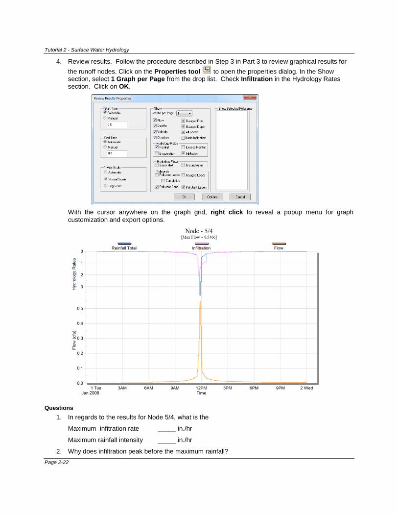
4. Review results. Follow the procedure described in Step 3 in Part 3 to review graphical results for the runoff nodes. Click on the Properties tool to open the properties dialog. In the Show section, select 1 Graph per Page from the drop list. Check Infiltration in the Hydrology Rates section. Click on OK.
With the cursor anywhere on the graph grid, right click to reveal a popup menu for graph customization and export options.
Questions 1. In regards to the results for Node 5/4, what is the
Maximum infitration rate _____ in./hr
Maximum rainfall intensity _____ in./hr
2. Why does infiltration peak before the maximum rainfall? Page 2-22
Tutorial 2 - Surface Water Hydrology
Part 5 – The Output File In the program a variety of tools are available for examining model results.
Level: Beginner
Objectives: Introduce the steps required to: • Add XP Tables to an existing database • Review results in the output file
Time: 0.5 hours
Data files: Yarra24.xp (same as file developed in Part 4)
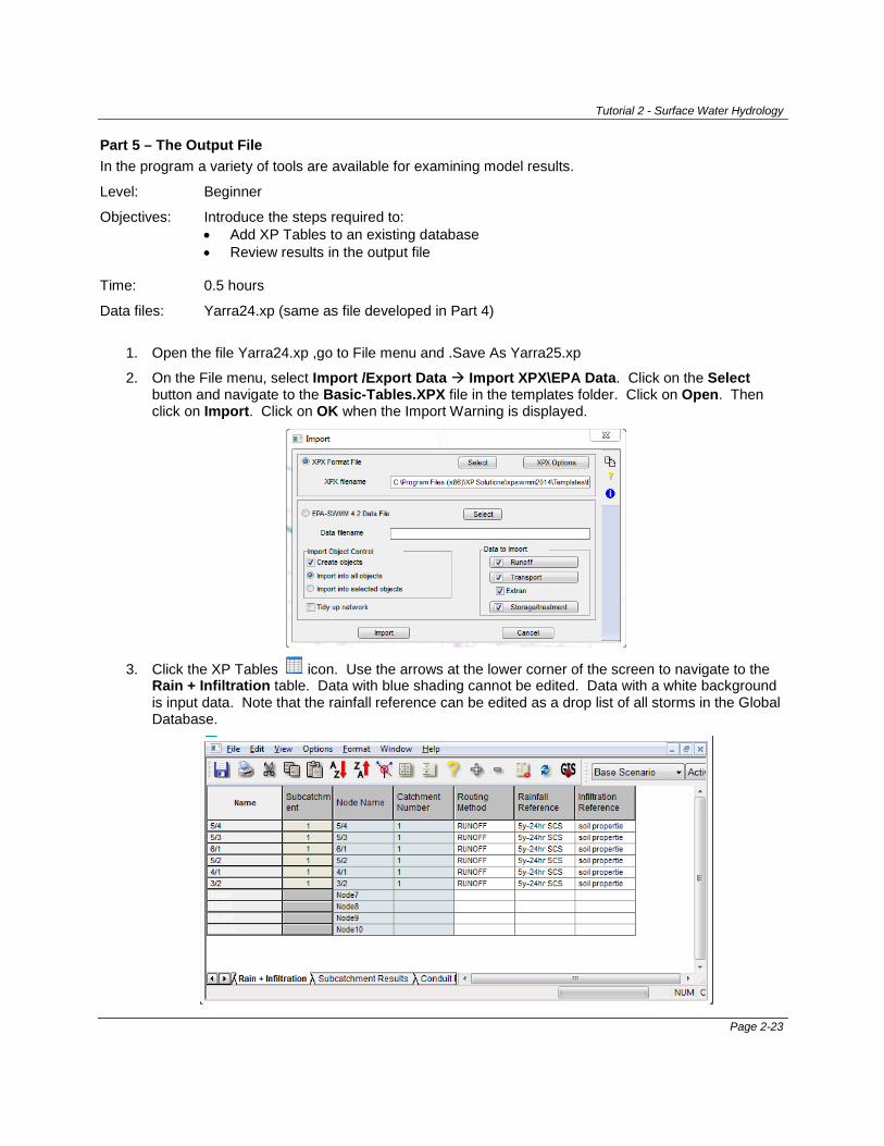
1. Open the file Yarra24.xp ,go to File menu and .Save As Yarra25.xp
2. On the File menu, select Import /Export Data Import XPX\EPA Data. Click on the Select button and navigate to the Basic-Tables.XPX file in the templates folder. Click on Open. Then click on Import. Click on OK when the Import Warning is displayed.
3. Click the XP Tables icon. Use the arrows at the lower corner of the screen to navigate to the Rain + Infiltration table. Data with blue shading cannot be edited. Data with a white background is input data. Note that the rainfall reference can be edited as a drop list of all storms in the Global Database.
Page 2-23
Tutorial 2 - Surface Water Hydrology
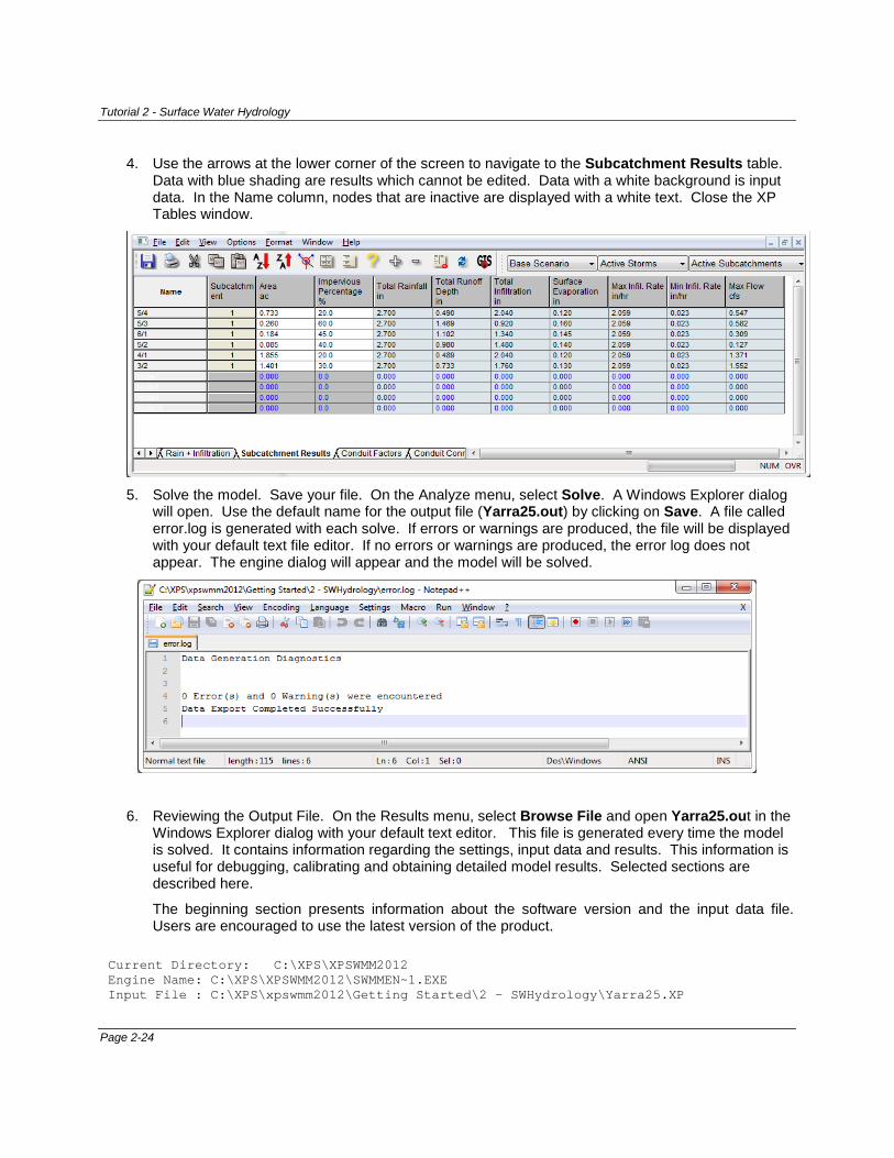
4. Use the arrows at the lower corner of the screen to navigate to the Subcatchment Results table. Data with blue shading are results which cannot be edited. Data with a white background is input data. In the Name column, nodes that are inactive are displayed with a white text. Close the XP Tables window.
5. Solve the model. Save your file. On the Analyze menu, select Solve. A Windows Explorer dialog
will open. Use the default name for the output file (Yarra25.out) by clicking on Save. A file called error.log is generated with each solve. If errors or warnings are produced, the file will be displayed with your default text file editor. If no errors or warnings are produced, the error log does not appear. The engine dialog will appear and the model will be solved.
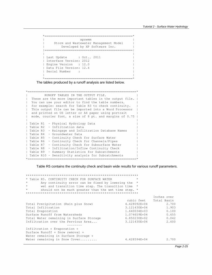
6. Reviewing the Output File. On the Results menu, select Browse File and open Yarra25.out in the Windows Explorer dialog with your default text editor. This file is generated every time the model is solved. It contains information regarding the settings, input data and results. This information is useful for debugging, calibrating and obtaining detailed model results. Selected sections are described here.
The beginning section presents information about the software version and the input data file. Users are encouraged to use the latest version of the product.
Current Directory: C:\XPS\XPSWMM2012 Engine Name: C:\XPS\XPSWMM2012\SWMMEN~1.EXE Input File : C:\XPS\xpswmm2012\Getting Started\2 - SWHydrology\Yarra25.XP
Page 2-24
Tutorial 2 - Surface Water Hydrology
*===============================================* | xpswmm | | Storm and Wastewater Management Model | | Developed by XP Software Inc. | |===============================================| | | | Last Update : Oct., 2011 | | Interface Version: 2012 | | Engine Version : 12.0 | | Data File Version: 12.4 | | Serial Number : | | | *===============================================*
The tables produced by a runoff analysis are listed below. *==========================================================* | RUNOFF TABLES IN THE OUTPUT FILE. | | These are the more important tables in the output file. | | You can use your editor to find the table numbers, | | for example: search for Table R3 to check continuity. | | This output file can be imported into a Word Processor | | and printed on US letter or A4 paper using portrait | | mode, courier font, a size of 8 pt. and margins of 0.75 | | | | Table R1 - Physical Hydrology Data | | Table R2 - Infiltration data | | Table R3 - Raingage and Infiltration Database Names | | Table R4 - Groundwater Data | | Table R5 - Continuity Check for Surface Water | | Table R6 - Continuity Check for Channels/Pipes | | Table R7 - Continuity Check for Subsurface Water | | Table R8 - Infiltration/Inflow Continuity Check | | Table R9 - Summary Statistics for Subcatchments | | Table R10 - Sensitivity analysis for Subcatchments | *==========================================================*
Table R5 contains the continuity check and basin wide results for various runoff parameters. ************************************************************ * Table R5. CONTINUITY CHECK FOR SURFACE WATER * * Any continuity error can be fixed by lowering the * * wet and transition time step. The transition time * * should not be much greater than the wet time step. * ************************************************************ Inches over cubic feet Total Basin Total Precipitation (Rain plus Snow) 4.428092E+04 2.700 Total Infiltration 3.121430E+04 1.903 Total Evaporation 1.640034E+03 0.100 Surface Runoff from Watersheds 1.074659E+04 0.655 Total Water remaining in Surface Storage 6.850230E+02 0.042 Infiltration over the Pervious Area... 3.121430E+04 2.600 -------- Infiltration + Evaporation + Surface Runoff + Snow removal + Water remaining in Surface Storage + Water remaining in Snow Cover......... 4.428594E+04 2.700
Page 2-25
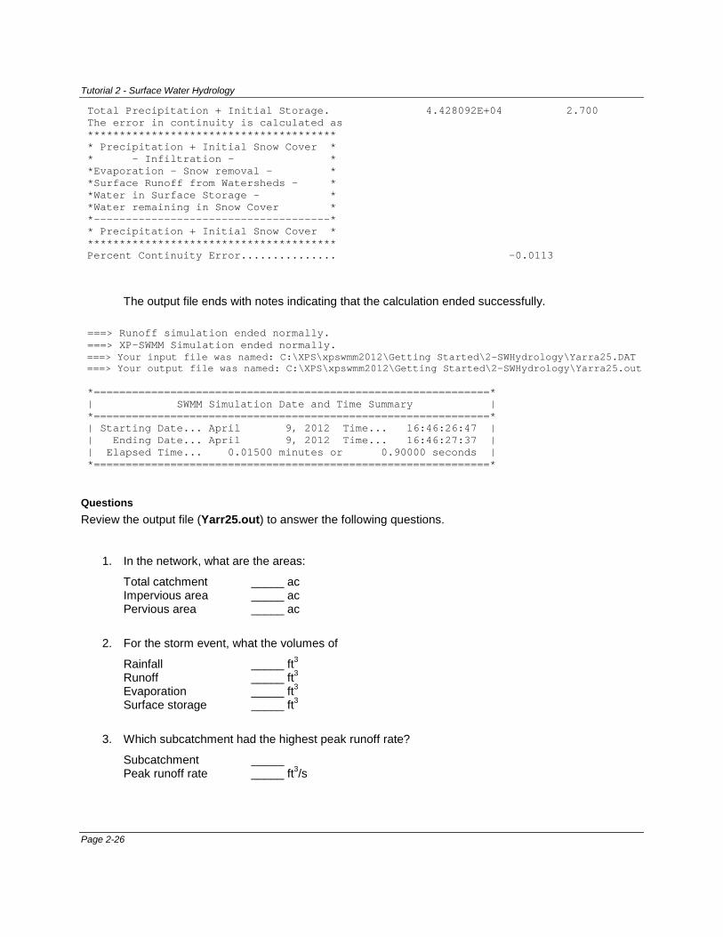
Tutorial 2 - Surface Water Hydrology
Total Precipitation + Initial Storage. 4.428092E+04 2.700 The error in continuity is calculated as *************************************** * Precipitation + Initial Snow Cover * * - Infiltration - * *Evaporation - Snow removal - * *Surface Runoff from Watersheds - * *Water in Surface Storage - * *Water remaining in Snow Cover * *-------------------------------------* * Precipitation + Initial Snow Cover * *************************************** Percent Continuity Error............... -0.0113
The output file ends with notes indicating that the calculation ended successfully. ===> Runoff simulation ended normally. ===> XP-SWMM Simulation ended normally. ===> Your input file was named: C:\XPS\xpswmm2012\Getting Started\2-SWHydrology\Yarra25.DAT ===> Your output file was named: C:\XPS\xpswmm2012\Getting Started\2-SWHydrology\Yarra25.out *==============================================================* | SWMM Simulation Date and Time Summary | *==============================================================* | Starting Date... April 9, 2012 Time... 16:46:26:47 | | Ending Date... April 9, 2012 Time... 16:46:27:37 | | Elapsed Time... 0.01500 minutes or 0.90000 seconds | *==============================================================*
Questions Review the output file (Yarr25.out) to answer the following questions.
1. In the network, what are the areas:
Total catchment _____ ac Impervious area _____ ac Pervious area _____ ac
2. For the storm event, what the volumes of
Rainfall _____ ft3 Runoff _____ ft3 Evaporation _____ ft3 Surface storage _____ ft3
3. Which subcatchment had the highest peak runoff rate?
Subcatchment _____ Peak runoff rate _____ ft3/s
Page 2-26
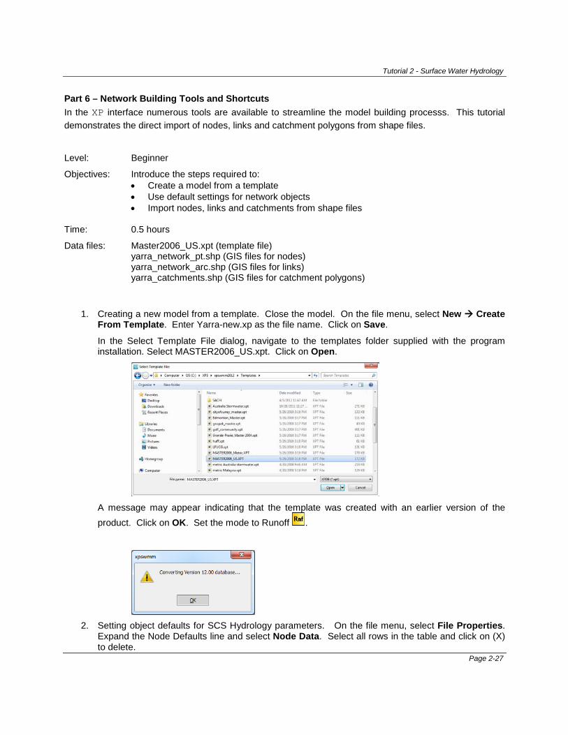
Tutorial 2 - Surface Water Hydrology
Part 6 – Network Building Tools and Shortcuts In the XP interface numerous tools are available to streamline the model building processs. This tutorial demonstrates the direct import of nodes, links and catchment polygons from shape files.
Level: Beginner
Objectives: Introduce the steps required to: • Create a model from a template • Use default settings for network objects • Import nodes, links and catchments from shape files
Time: 0.5 hours
Data files: Master2006_US.xpt (template file) yarra_network_pt.shp (GIS files for nodes) yarra_network_arc.shp (GIS files for links) yarra_catchments.shp (GIS files for catchment polygons)
1. Creating a new model from a template. Close the model. On the file menu, select New Create From Template. Enter Yarra-new.xp as the file name. Click on Save.
In the Select Template File dialog, navigate to the templates folder supplied with the program installation. Select MASTER2006_US.xpt. Click on Open.
A message may appear indicating that the template was created with an earlier version of the product. Click on OK. Set the mode to Runoff .
2. Setting object defaults for SCS Hydrology parameters. On the file menu, select File Properties.
Expand the Node Defaults line and select Node Data. Select all rows in the table and click on (X) to delete.
Page 2-27
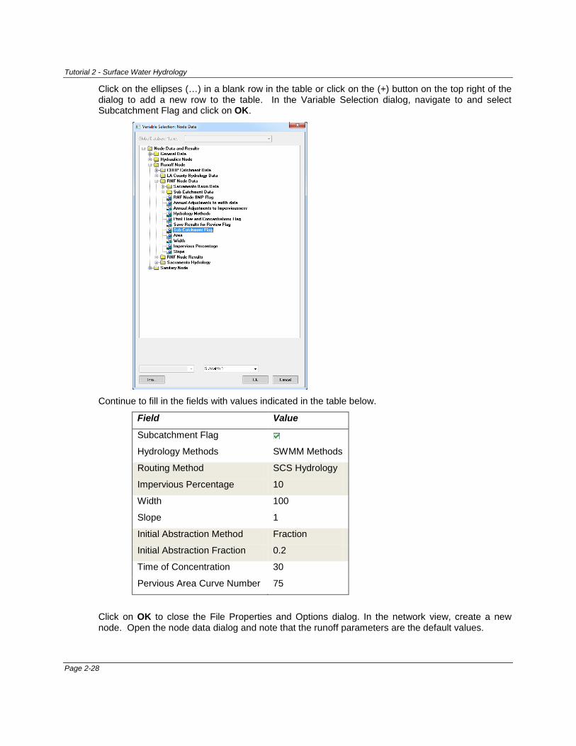
Tutorial 2 - Surface Water Hydrology
Click on the ellipses (…) in a blank row in the table or click on the (+) button on the top right of the dialog to add a new row to the table. In the Variable Selection dialog, navigate to and select Subcatchment Flag and click on OK.
Continue to fill in the fields with values indicated in the table below.
Field Value
Subcatchment Flag Hydrology Methods SWMM Methods
Routing Method SCS Hydrology
Impervious Percentage 10
Width 100
Slope 1
Initial Abstraction Method Fraction
Initial Abstraction Fraction 0.2
Time of Concentration 30
Pervious Area Curve Number 75
Click on OK to close the File Properties and Options dialog. In the network view, create a new node. Open the node data dialog and note that the runoff parameters are the default values.
Page 2-28
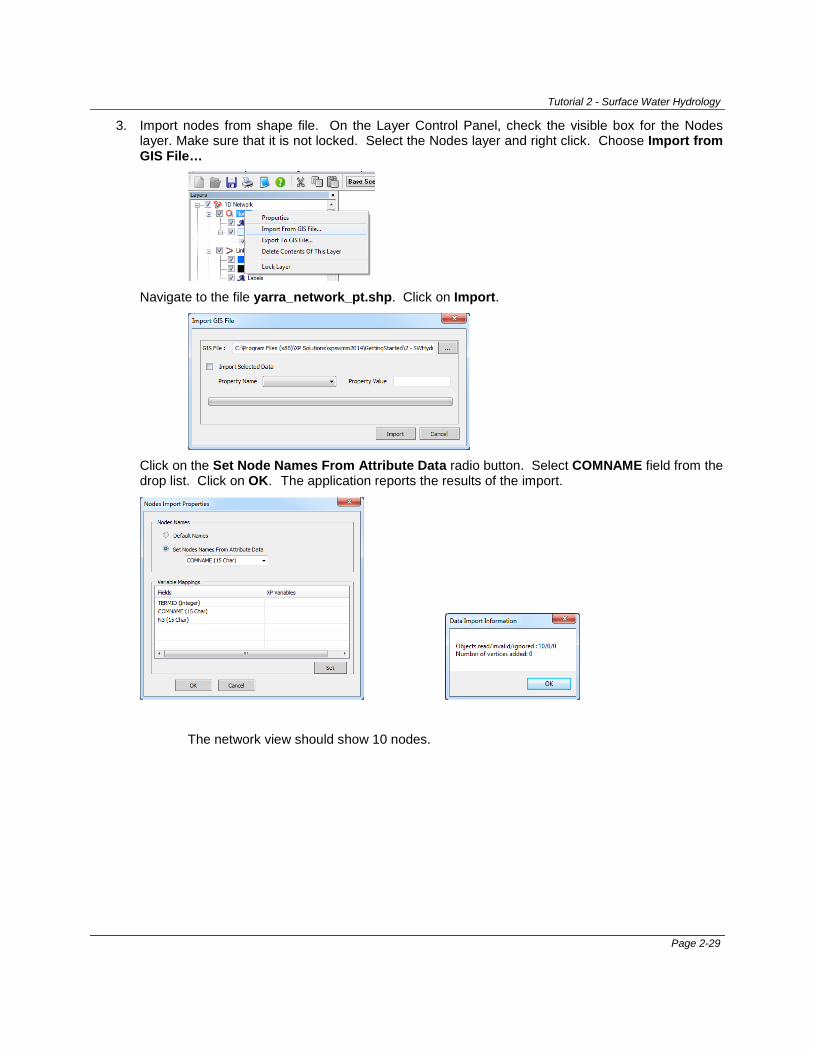
Tutorial 2 - Surface Water Hydrology
3. Import nodes from shape file. On the Layer Control Panel, check the visible box for the Nodes layer. Make sure that it is not locked. Select the Nodes layer and right click. Choose Import from GIS File…
Navigate to the file yarra_network_pt.shp. Click on Import.
Click on the Set Node Names From Attribute Data radio button. Select COMNAME field from the drop list. Click on OK. The application reports the results of the import.
The network view should show 10 nodes.
Page 2-29
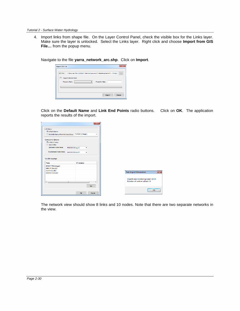
Tutorial 2 - Surface Water Hydrology
4. Import links from shape file. On the Layer Control Panel, check the visible box for the Links layer. Make sure the layer is unlocked. Select the Links layer. Right click and choose Import from GIS File… from the popup menu.
Navigate to the file yarra_network_arc.shp. Click on Import.
Click on the Default Name and Link End Points radio buttons. Click on OK. The application reports the results of the import.
The network view should show 8 links and 10 nodes. Note that there are two separate networks in the view.
Page 2-30
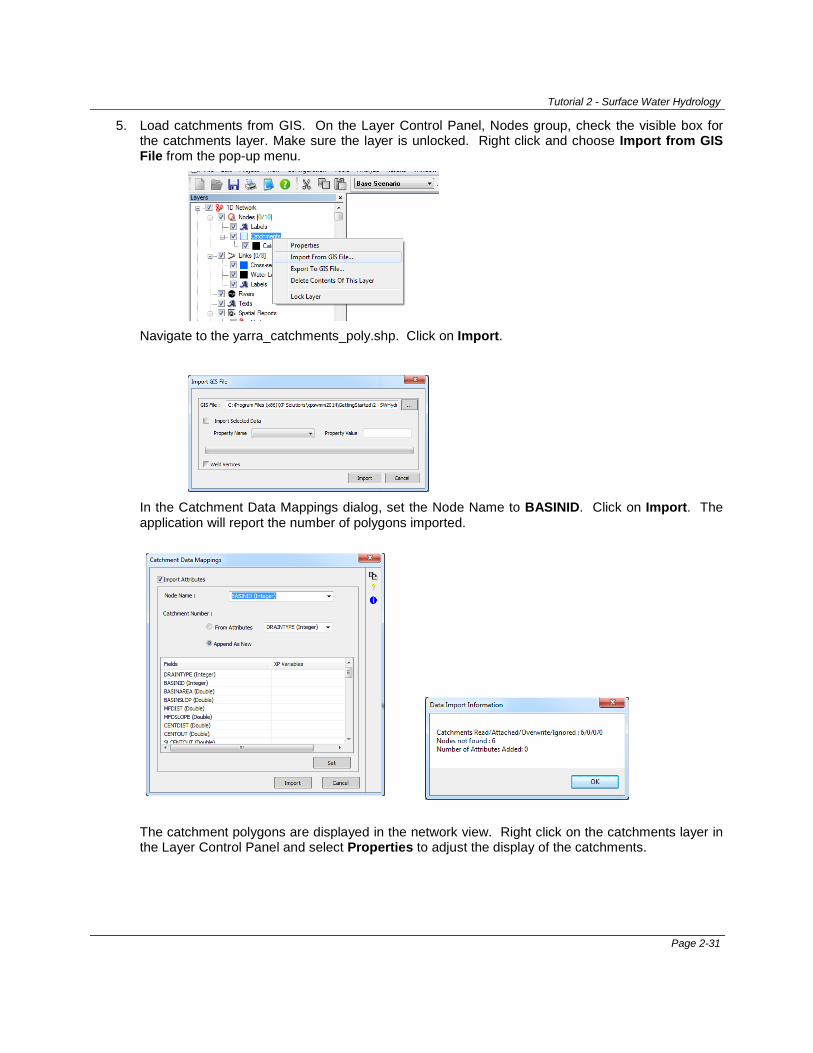
Tutorial 2 - Surface Water Hydrology
5. Load catchments from GIS. On the Layer Control Panel, Nodes group, check the visible box for the catchments layer. Make sure the layer is unlocked. Right click and choose Import from GIS File from the pop-up menu.
Navigate to the yarra_catchments_poly.shp. Click on Import.
In the Catchment Data Mappings dialog, set the Node Name to BASINID. Click on Import. The application will report the number of polygons imported.
The catchment polygons are displayed in the network view. Right click on the catchments layer in the Layer Control Panel and select Properties to adjust the display of the catchments.
Page 2-31
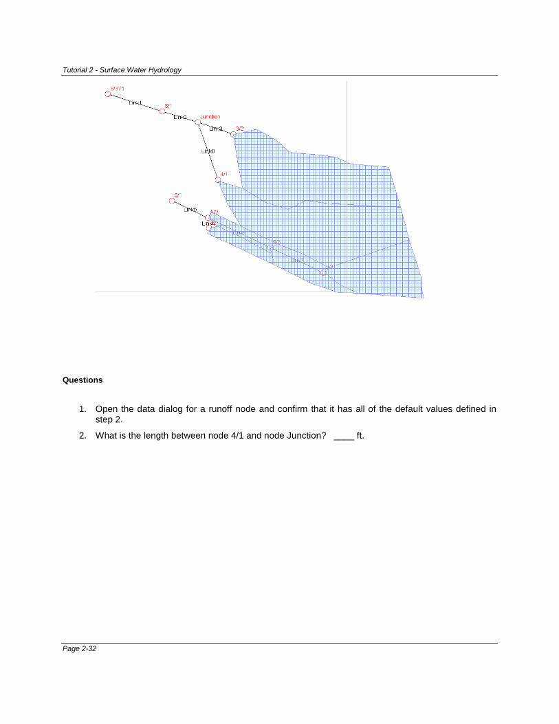
Tutorial 2 - Surface Water Hydrology
Questions
1. Open the data dialog for a runoff node and confirm that it has all of the default values defined in step 2.
2. What is the length between node 4/1 and node Junction? ____ ft.
Page 2-32
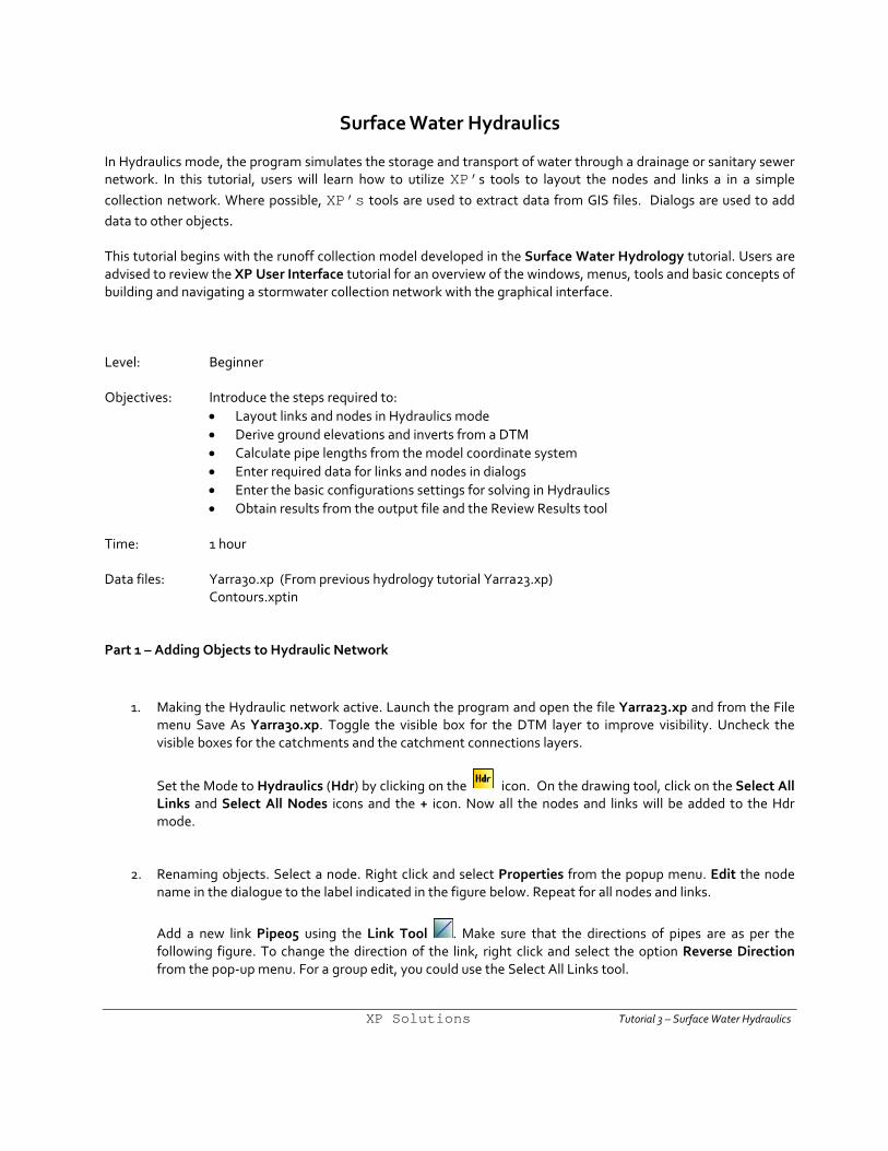
Surface Water Hydraulics
In Hydraulics mode, the program simulates the storage and transport of water through a drainage or sanitary sewer network. In this tutorial, users will learn how to utilize XP’s tools to layout the nodes and links a in a simple collection network. Where possible, XP’s tools are used to extract data from GIS files. Dialogs are used to add data to other objects.
This tutorial begins with the runoff collection model developed in the Surface Water Hydrology tutorial. Users are advised to review the XP User Interface tutorial for an overview of the windows, menus, tools and basic concepts of building and navigating a stormwater collection network with the graphical interface.
Level: Beginner
Objectives: Introduce the steps required to: • Layout links and nodes in Hydraulics mode • Derive ground elevations and inverts from a DTM • Calculate pipe lengths from the model coordinate system • Enter required data for links and nodes in dialogs • Enter the basic configurations settings for solving in Hydraulics • Obtain results from the output file and the Review Results tool
Time: 1 hour
Data files: Yarra30.xp (From previous hydrology tutorial Yarra23.xp) Contours.xptin
Part 1 – Adding Objects to Hydraulic Network
1. Making the Hydraulic network active. Launch the program and open the file Yarra23.xp and from the File menu Save As Yarra30.xp. Toggle the visible box for the DTM layer to improve visibility. Uncheck the visible boxes for the catchments and the catchment connections layers.
Set the Mode to Hydraulics (Hdr) by clicking on the icon. On the drawing tool, click on the Select All Links and Select All Nodes icons and the + icon. Now all the nodes and links will be added to the Hdr mode.
2. Renaming objects. Select a node. Right click and select Properties from the popup menu. Edit the node
name in the dialogue to the label indicated in the figure below. Repeat for all nodes and links.
Add a new link Pipe05 using the Link Tool . Make sure that the directions of pipes are as per the following figure. To change the direction of the link, right click and select the option Reverse Direction from the pop-up menu. For a group edit, you could use the Select All Links tool.
XP Solutions Tutorial 3 – Surface Water Hydraulics
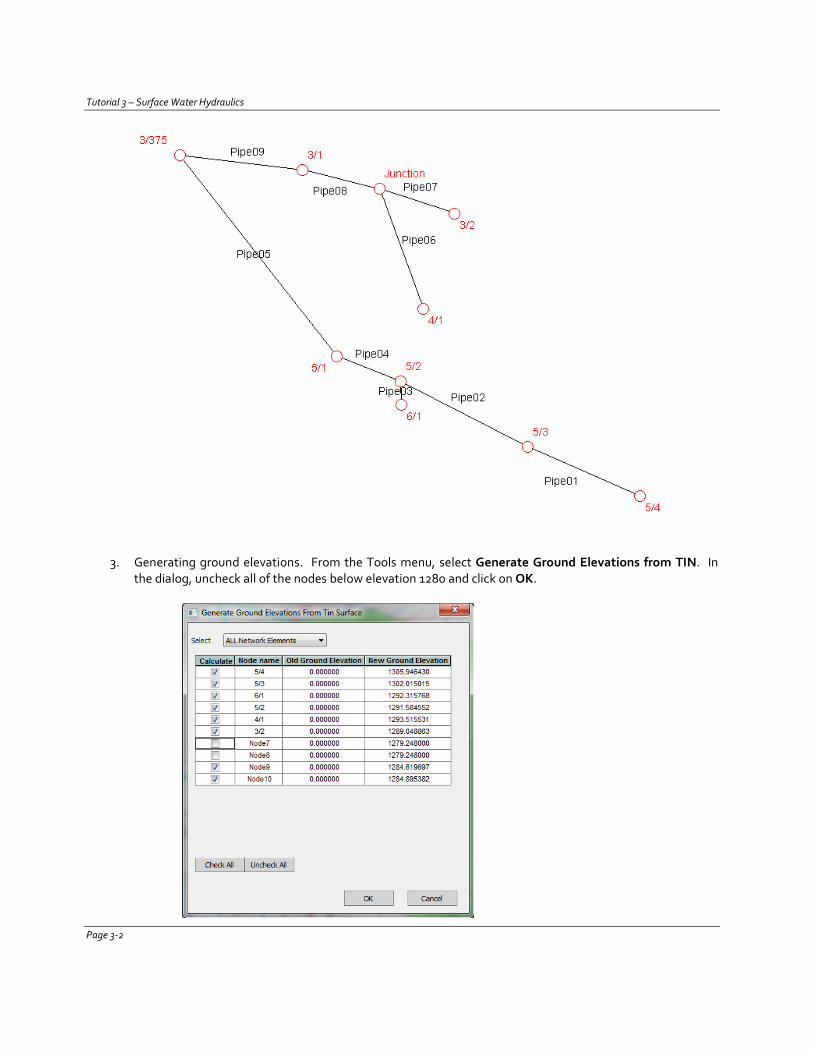
Tutorial 3 – Surface Water Hydraulics
3. Generating ground elevations. From the Tools menu, select Generate Ground Elevations from TIN. In the dialog, uncheck all of the nodes below elevation 1280 and click on OK.
Page 3-2
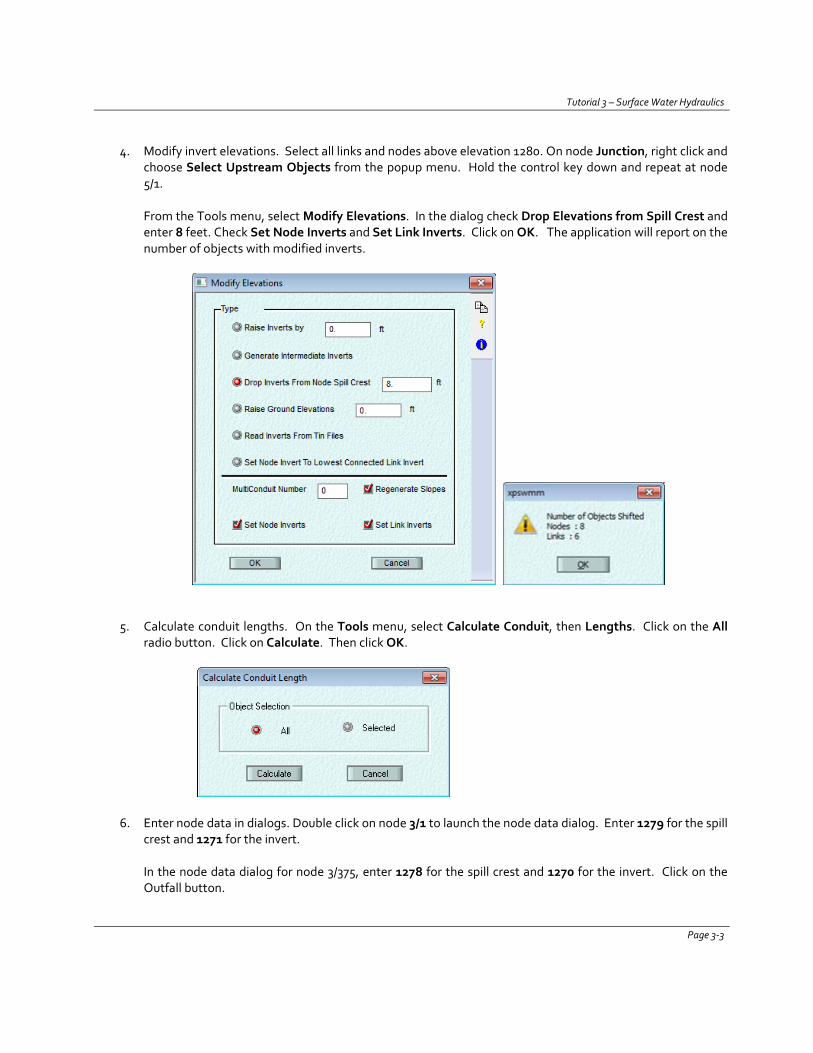
Tutorial 3 – Surface Water Hydraulics
4. Modify invert elevations. Select all links and nodes above elevation 1280. On node Junction, right click and
choose Select Upstream Objects from the popup menu. Hold the control key down and repeat at node 5/1.
From the Tools menu, select Modify Elevations. In the dialog check Drop Elevations from Spill Crest and enter 8 feet. Check Set Node Inverts and Set Link Inverts. Click on OK. The application will report on the number of objects with modified inverts.
5. Calculate conduit lengths. On the Tools menu, select Calculate Conduit, then Lengths. Click on the All radio button. Click on Calculate. Then click OK.
6. Enter node data in dialogs. Double click on node 3/1 to launch the node data dialog. Enter 1279 for the spill crest and 1271 for the invert.
In the node data dialog for node 3/375, enter 1278 for the spill crest and 1270 for the invert. Click on the Outfall button.
Page 3-3
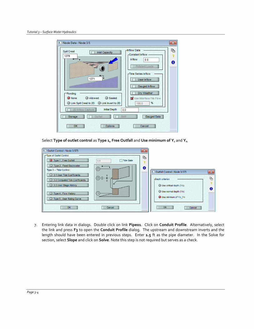
Tutorial 3 – Surface Water Hydraulics
Select Type of outlet control as Type 1, Free Outfall and Use minimum of Yc and Yn.
7. Entering link data in dialogs. Double click on link Pipe01. Click on Conduit Profile. Alternatively, select
the link and press F3 to open the Conduit Profile dialog. The upstream and downstream inverts and the length should have been entered in previous steps. Enter 1.5 ft as the pipe diameter. In the Solve for section, select Slope and click on Solve. Note this step is not required but serves as a check.
Page 3-4
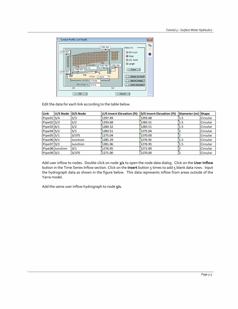
Tutorial 3 – Surface Water Hydraulics
Edit the data for each link according to the table below.
Link U/S Node D/S Node U/S Invert Elevation (ft) D/S Invert Elevation (ft) Diameter (m) ShapePipe01 5/4 5/3 1297.49 1293.68 1.5 CircularPipe02 5/3 5/2 1293.68 1283.51 1.5 CircularPipe03 6/1 5/2 1284.32 1283.51 1.5 CircularPipe04 5/2 5/1 1283.51 1275.04 2 CircularPipe05 5/1 3/375 1275.04 1270.00 2 CircularPipe06 4/1 Junction 1285.29 1276.95 1.5 CircularPipe07 3/2 Junction 1281.06 1276.95 1.5 CircularPipe08 Junction 3/1 1276.95 1271.00 2 CircularPipe09 3/1 3/375 1271.00 1270.00 2 Circular
Add user inflow to nodes. Double-click on node 3/1 to open the node data dialog. Click on the User Inflow button in the Time Series Inflow section. Click on the Insert button 5 times to add 5 blank data rows. Input the hydrograph data as shown in the figure below. This data represents inflow from areas outside of the Yarra model.
Add the same user inflow hydrograph to node 5/1.
Page 3-5
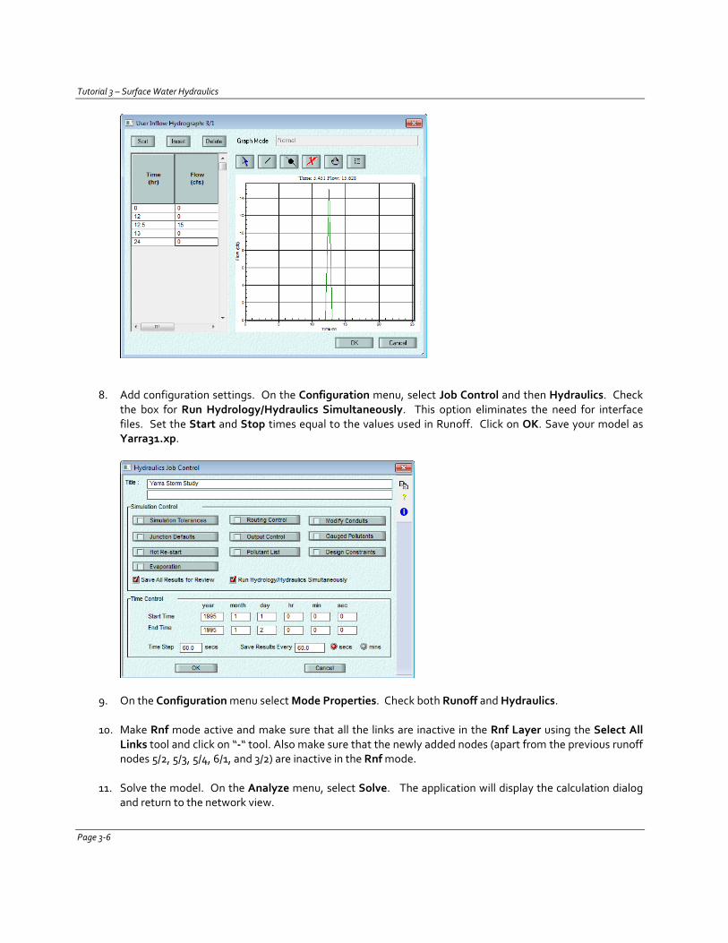
Tutorial 3 – Surface Water Hydraulics
8. Add configuration settings. On the Configuration menu, select Job Control and then Hydraulics. Check the box for Run Hydrology/Hydraulics Simultaneously. This option eliminates the need for interface files. Set the Start and Stop times equal to the values used in Runoff. Click on OK. Save your model as Yarra31.xp.
9. On the Configuration menu select Mode Properties. Check both Runoff and Hydraulics.
10. Make Rnf mode active and make sure that all the links are inactive in the Rnf Layer using the Select All Links tool and click on “-“ tool. Also make sure that the newly added nodes (apart from the previous runoff nodes 5/2, 5/3, 5/4, 6/1, and 3/2) are inactive in the Rnf mode.
11. Solve the model. On the Analyze menu, select Solve. The application will display the calculation dialog and return to the network view.
Page 3-6
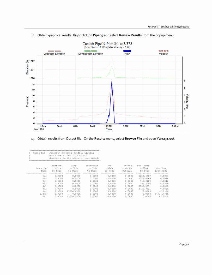
Tutorial 3 – Surface Water Hydraulics
12. Obtain graphical results. Right click on Pipe09 and select Review Results from the popup menu.
13. Obtain results from Output file. On the Results menu, select Browse File and open Yarra31.out. *===================================================* | Table E19 - Junction Inflow & Outflow Listing | | Units are either ft^3 or m^3 | | depending on the units in your model.| *===================================================* Constant User Interface DWF Inflow RNF Layer Junction Inflow Inflow Inflow Inlow through Inflow Outflow Name to Node to Node to Node to Node Outfall to Node from Node --------------- ---------- ----------- ----------- ----------- ----------- ----------- ----------- 5/4 0.0000 0.0000 0.0000 0.0000 0.0000 1289.4967 0.0001 5/3 0.0000 0.0000 0.0000 0.0000 0.0000 1385.6769 0.0029 6/1 0.0000 0.0000 0.0000 0.0000 0.0000 735.9402 0.0042 5/2 0.0000 0.0000 0.0000 0.0000 0.0000 302.2295 0.0318 4/1 0.0000 0.0000 0.0000 0.0000 0.0000 3289.4391 0.0018 3/2 0.0000 0.0000 0.0000 0.0000 0.0000 3726.3621 0.0019 3/1 0.0000 27000.0000 0.0000 0.0000 0.0000 0.0000 -2.9398 3/375 0.0000 0.0000 0.0000 0.0000 0.0000 0.0000 64726.4735 5/1 0.0000 27000.0000 0.0000 0.0000 0.0000 0.0000 -6.0739
Page 3-7

Tutorial 3 – Surface Water Hydraulics
Questions
Review the output file (Yarra31.out) to answer the following questions.
1. What is the total outflow at node 3/375? (Hint: Table E19.) _________
2. What is the maximum flow in link Pipe09? (Hint: Table E15a). _________
Page 3-8
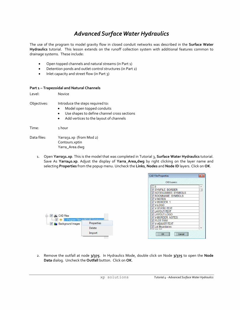
Advanced Surface Water Hydraulics
The use of the program to model gravity flow in closed conduit networks was described in the Surface Water Hydraulics tutorial. This lesson extends on the runoff collection system with additional features common to drainage systems. These include:
• Open topped channels and natural streams (in Part 1) • Detention ponds and outlet control structures (in Part 2) • Inlet capacity and street flow (in Part 3)
Part 1 – Trapezoidal and Natural Channels
Level: Novice
Objectives: Introduce the steps required to: • Model open topped conduits • Use shapes to define channel cross sections • Add vertices to the layout of channels
Time: 1 hour
Data files: Yarra31.xp (from Mod 2) Contours.xptin Yarra_Area.dwg
1. Open Yarra31.xp. This is the model that was completed in Tutorial 3, Surface Water Hydraulics tutorial. Save As Yarra40.xp. Adjust the display of Yarra_Area,dwg by right clicking on the layer name and selecting Properties from the popup menu. Uncheck the Links, Nodes and Node ID layers. Click on OK.
2. Remove the outfall at node 3/375. In Hydraulics Mode, double click on Node 3/375 to open the Node Data dialog. Uncheck the Outfall button. Click on OK.
xp solutions Tutorial 4 - Advanced Surface Water Hydraulics
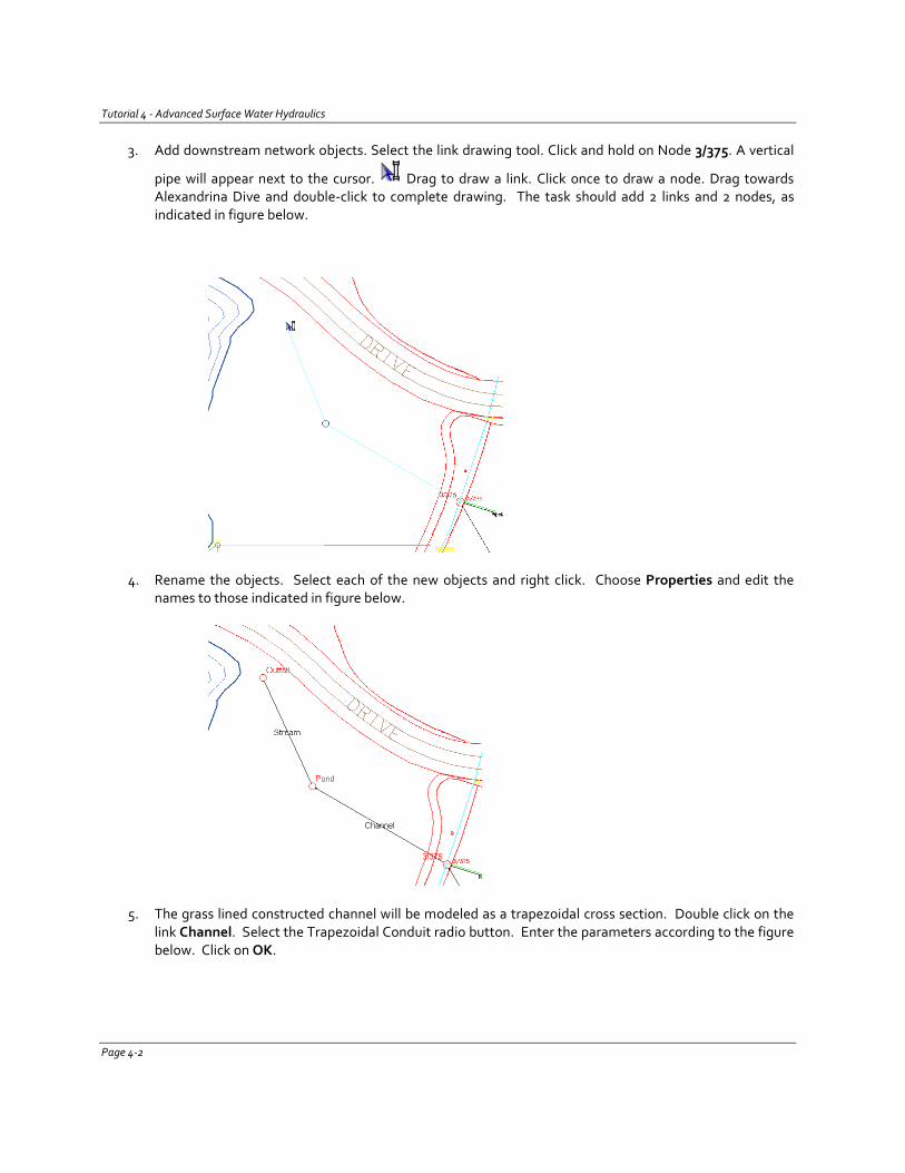
Tutorial 4 - Advanced Surface Water Hydraulics
3. Add downstream network objects. Select the link drawing tool. Click and hold on Node 3/375. A vertical
pipe will appear next to the cursor. Drag to draw a link. Click once to draw a node. Drag towards Alexandrina Dive and double-click to complete drawing. The task should add 2 links and 2 nodes, as indicated in figure below.
4. Rename the objects. Select each of the new objects and right click. Choose Properties and edit the names to those indicated in figure below.
5. The grass lined constructed channel will be modeled as a trapezoidal cross section. Double click on the link Channel. Select the Trapezoidal Conduit radio button. Enter the parameters according to the figure below. Click on OK.
Page 4-2
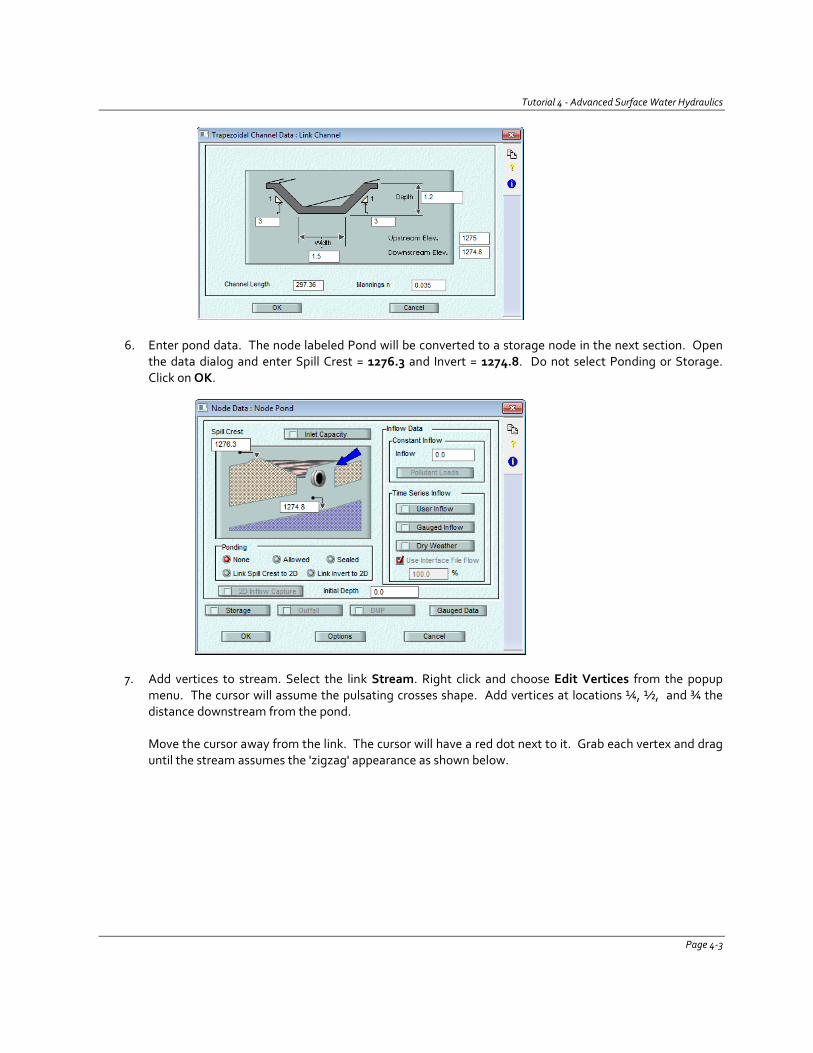
Tutorial 4 - Advanced Surface Water Hydraulics
6. Enter pond data. The node labeled Pond will be converted to a storage node in the next section. Open the data dialog and enter Spill Crest = 1276.3 and Invert = 1274.8. Do not select Ponding or Storage. Click on OK.
7. Add vertices to stream. Select the link Stream. Right click and choose Edit Vertices from the popup
menu. The cursor will assume the pulsating crosses shape. Add vertices at locations ¼, ½, and ¾ the distance downstream from the pond.
Move the cursor away from the link. The cursor will have a red dot next to it. Grab each vertex and drag until the stream assumes the 'zigzag' appearance as shown below.
Page 4-3
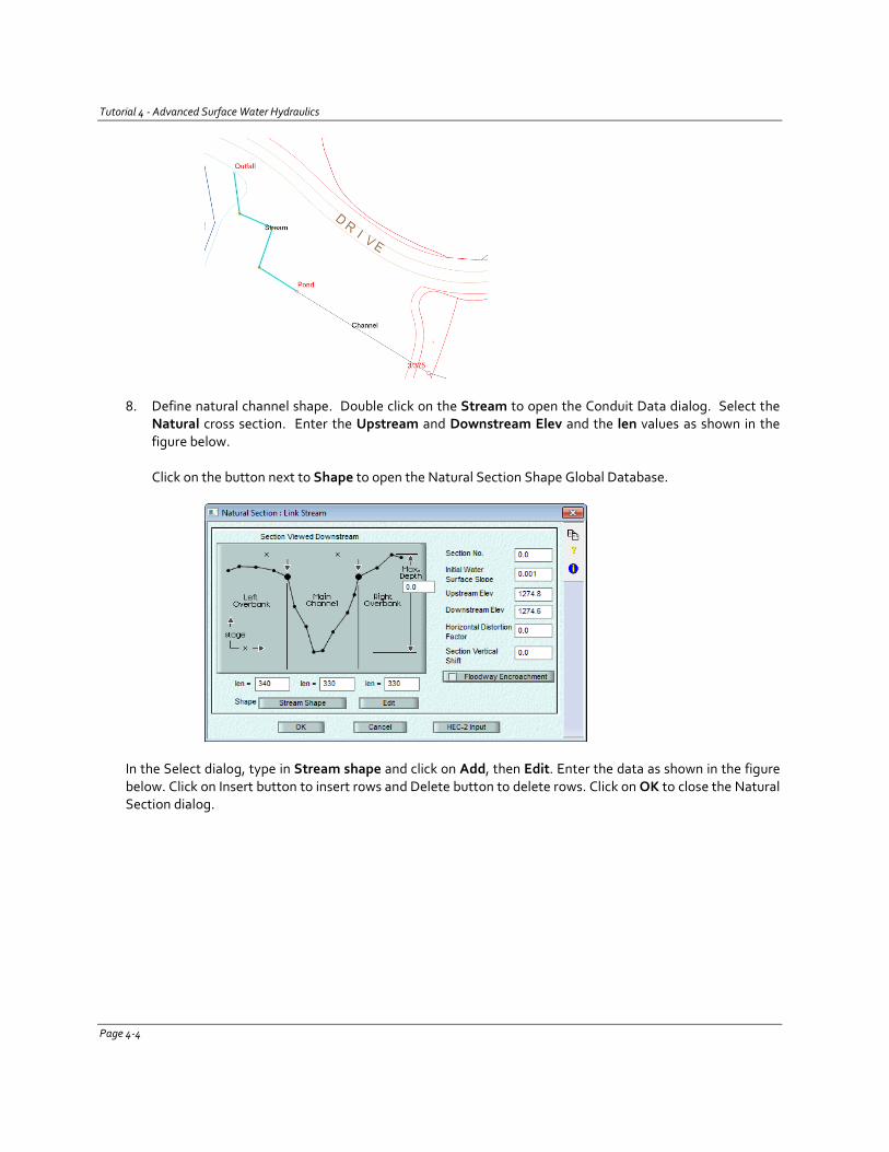
Tutorial 4 - Advanced Surface Water Hydraulics
8. Define natural channel shape. Double click on the Stream to open the Conduit Data dialog. Select the Natural cross section. Enter the Upstream and Downstream Elev and the len values as shown in the figure below.
Click on the button next to Shape to open the Natural Section Shape Global Database.
In the Select dialog, type in Stream shape and click on Add, then Edit. Enter the data as shown in the figure below. Click on Insert button to insert rows and Delete button to delete rows. Click on OK to close the Natural Section dialog.
Page 4-4
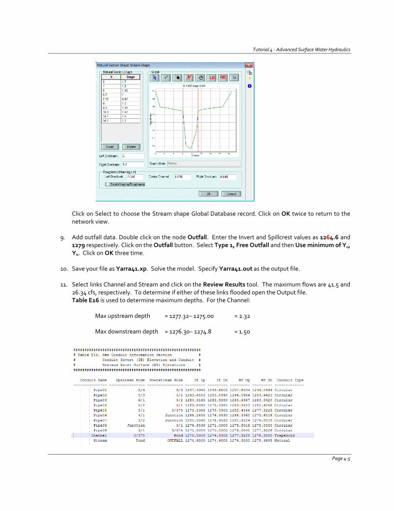
Tutorial 4 - Advanced Surface Water Hydraulics
Click on Select to choose the Stream shape Global Database record. Click on OK twice to return to the network view.
9. Add outfall data. Double click on the node Outfall. Enter the Invert and Spillcrest values as 1264.6 and 1279 respectively. Click on the Outfall button. Select Type 1, Free Outfall and then Use minimum of Yc, Yn. Click on OK three time.
10. Save your file as Yarra41.xp. Solve the model. Specify Yarra41.out as the output file.
11. Select links Channel and Stream and click on the Review Results tool. The maximum flows are 41.5 and
26.34 cfs, respectively. To determine if either of these links flooded open the Output file. Table E16 is used to determine maximum depths. For the Channel:
Max upstream depth = 1277.32– 1275.00 = 2.32
Max downstream depth = 1276.30– 1274.8 = 1.50
Page 4-5
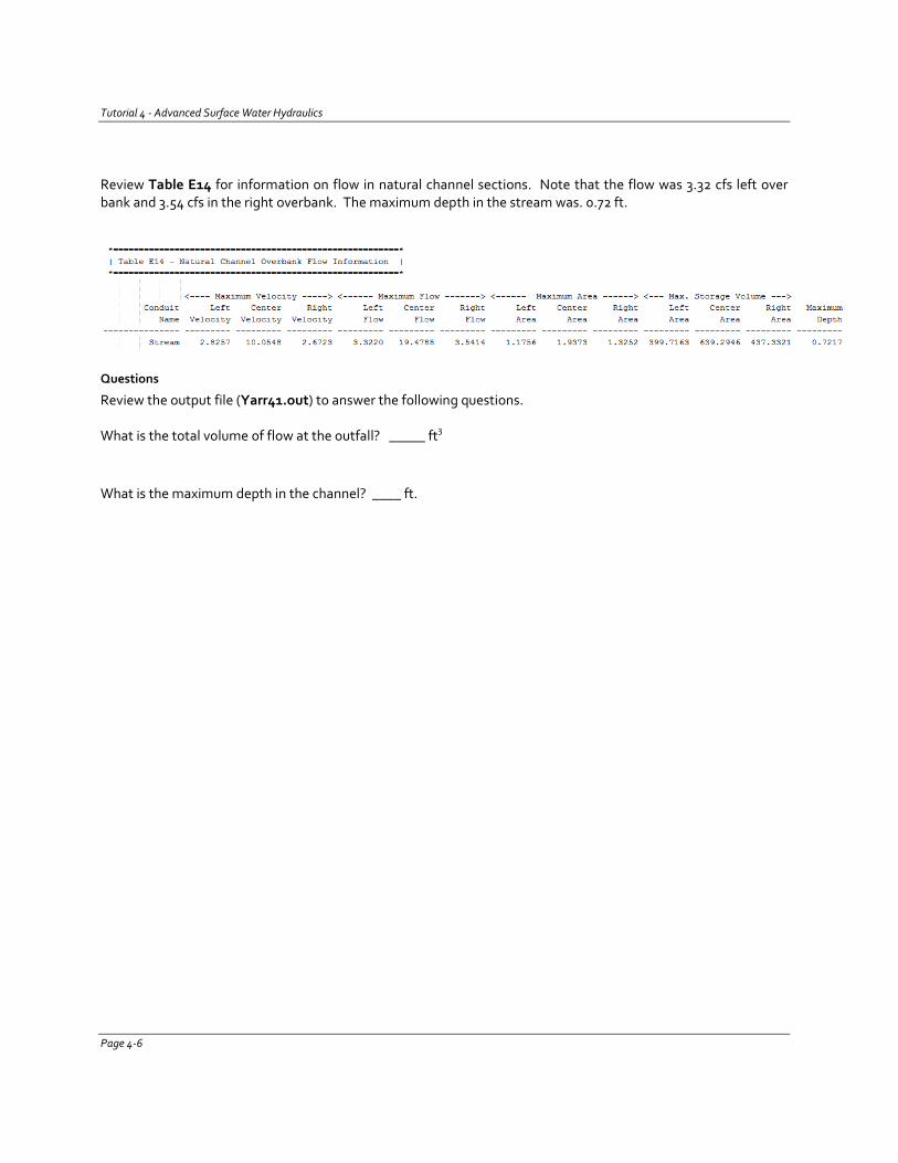
Tutorial 4 - Advanced Surface Water Hydraulics
Review Table E14 for information on flow in natural channel sections. Note that the flow was 3.32 cfs left over bank and 3.54 cfs in the right overbank. The maximum depth in the stream was. 0.72 ft.
Questions
Review the output file (Yarr41.out) to answer the following questions.
What is the total volume of flow at the outfall? _____ ft3
What is the maximum depth in the channel? ____ ft.
Page 4-6
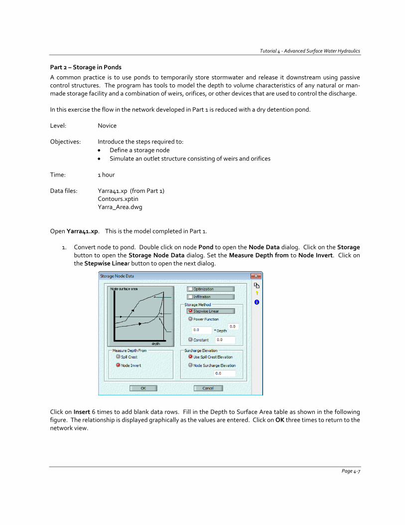
Tutorial 4 - Advanced Surface Water Hydraulics
Part 2 – Storage in Ponds
A common practice is to use ponds to temporarily store stormwater and release it downstream using passive control structures. The program has tools to model the depth to volume characteristics of any natural or man-made storage facility and a combination of weirs, orifices, or other devices that are used to control the discharge.
In this exercise the flow in the network developed in Part 1 is reduced with a dry detention pond.
Level: Novice
Objectives: Introduce the steps required to: • Define a storage node • Simulate an outlet structure consisting of weirs and orifices
Time: 1 hour
Data files: Yarra41.xp (from Part 1) Contours.xptin Yarra_Area.dwg
Open Yarra41.xp. This is the model completed in Part 1.
1. Convert node to pond. Double click on node Pond to open the Node Data dialog. Click on the Storage button to open the Storage Node Data dialog. Set the Measure Depth from to Node Invert. Click on the Stepwise Linear button to open the next dialog.
Click on Insert 6 times to add blank data rows. Fill in the Depth to Surface Area table as shown in the following figure. The relationship is displayed graphically as the values are entered. Click on OK three times to return to the network view.
Page 4-7
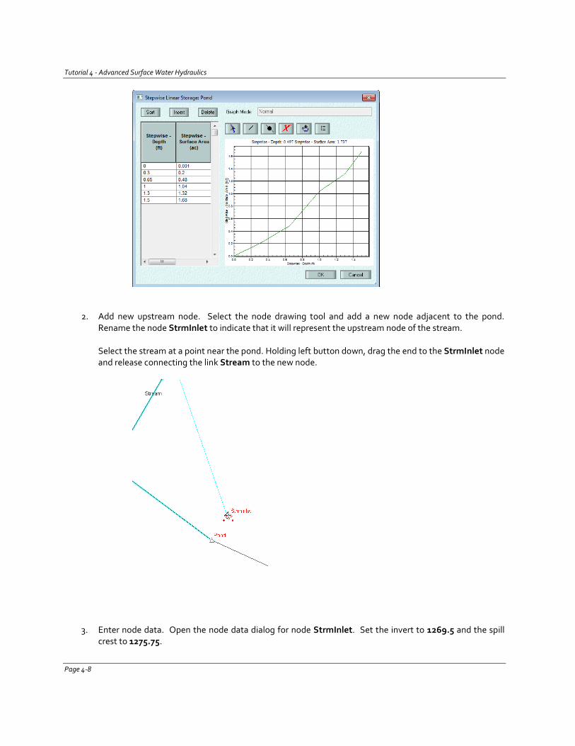
Tutorial 4 - Advanced Surface Water Hydraulics
2. Add new upstream node. Select the node drawing tool and add a new node adjacent to the pond. Rename the node StrmInlet to indicate that it will represent the upstream node of the stream.
Select the stream at a point near the pond. Holding left button down, drag the end to the StrmInlet node and release connecting the link Stream to the new node.
3. Enter node data. Open the node data dialog for node StrmInlet. Set the invert to 1269.5 and the spill crest to 1275.75.
Page 4-8
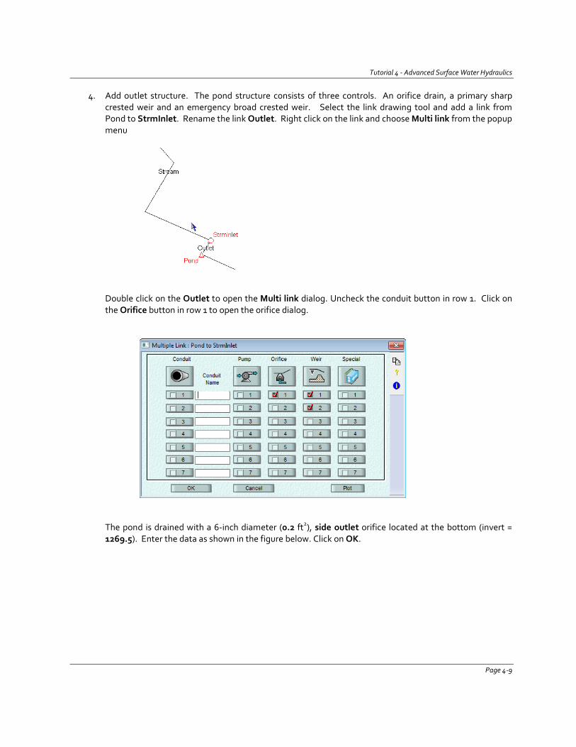
Tutorial 4 - Advanced Surface Water Hydraulics
4. Add outlet structure. The pond structure consists of three controls. An orifice drain, a primary sharp crested weir and an emergency broad crested weir. Select the link drawing tool and add a link from Pond to StrmInlet. Rename the link Outlet. Right click on the link and choose Multi link from the popup menu
Double click on the Outlet to open the Multi link dialog. Uncheck the conduit button in row 1. Click on the Orifice button in row 1 to open the orifice dialog.
The pond is drained with a 6-inch diameter (0.2 ft2), side outlet orifice located at the bottom (invert = 1269.5). Enter the data as shown in the figure below. Click on OK.
Page 4-9
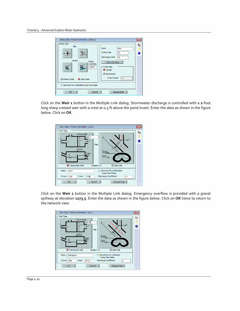
Tutorial 4 - Advanced Surface Water Hydraulics
Click on the Weir 1 button in the Multiple Link dialog. Stormwater discharge is controlled with a 2-foot long sharp crested weir with a crest at 0.5 ft above the pond invert. Enter the data as shown in the figure below. Click on OK.
Click on the Weir 2 button in the Multiple Link dialog. Emergency overflow is provided with a gravel spillway at elevation 1273.5. Enter the data as shown in the figure below. Click on OK twice to return to the network view.
Page 4-10
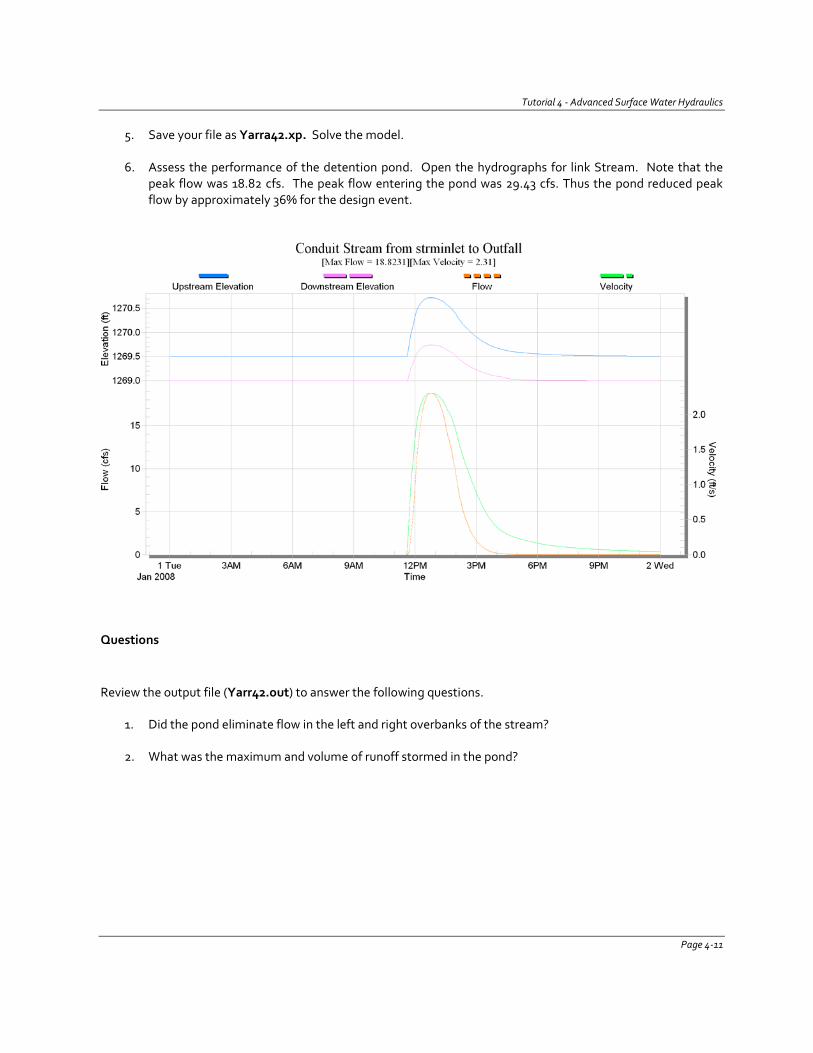
Tutorial 4 - Advanced Surface Water Hydraulics
5. Save your file as Yarra42.xp. Solve the model.
6. Assess the performance of the detention pond. Open the hydrographs for link Stream. Note that the peak flow was 18.82 cfs. The peak flow entering the pond was 29.43 cfs. Thus the pond reduced peak flow by approximately 36% for the design event.
Questions
Review the output file (Yarr42.out) to answer the following questions.
1. Did the pond eliminate flow in the left and right overbanks of the stream?
2. What was the maximum and volume of runoff stormed in the pond?
Page 4-11
Tutorial 4 - Advanced Surface Water Hydraulics
Part 3 – Street Flooding and Dual Drainage
Up to this point it has been assumed that hydraulic capacity is controlled only by the conduits in the network. In some cases, the capacity of grated and curb inlets restrict the amount of flow entering the collection system. The program provides a variety of options for defining an Inlet Rating Curve (IRC). The Inlet Rating Curve works as follows:
• If Ponding None and no surface conduits - Divert flow according to the selected IRC method and lose excess.
• If Ponding None with surface conduits - Divert flow according to the selected IRC method and excess distributed according to hydraulic properties of surface conduits. Any excess that cannot be re-distributed is lost.
• If Ponding Allowed and no surface conduits - Divert flow according to the selected IRC method with excess ponding at the surface. Ponded surface water is added to the diverted flow at a flow rate equivalent to the volume of surface water divided by the time step. The maximum total diverted flow however is capped at either the "Maximum Capacity" or at the maximum value entered in the rating curve so do not enter unrealistically high capture rates even if they have equally unrealistic approach flows because the approach flow is ignored when determining the absolute maximum allowed.
• If Ponding Allowed with surface conduits - Divert flow according to the selected IRC method and excess distributed according to hydraulic properties of surface conduits. Any excess that cannot be re-distributed is ponded as per 3 above with the total diverted flow increased accordingly.
• If the underground conduit has a constriction that causes reverse flow through the inlet then all the excess underground flow discharges back to the surface regardless of the inlet's maximum capacity (it blows its lid).
Whenever Inlet Capacity is turned on at a node, a second node is created, for computational purposes, with the text $I appended to the name. This new node is connected to the closed conduit and receives flow by an internal rating curve based on the inlet capacity. Results for this node are reported in the output file. In the Review Results graphical display, the new node is labeled as [Subsurface]. In Part 3, the inlet capacity feature will be used to control flow in conduits and excess flow will be routed in surface streets. Level: Novice
Objectives: Introduce the steps required to: • Define an inlet rating curve • Route excess flow along a street modeled as a multilink
Time: 1 hour
Data files: Yarra42.xp Contours.xptin Yarra_Area.dwg
Page 4-12
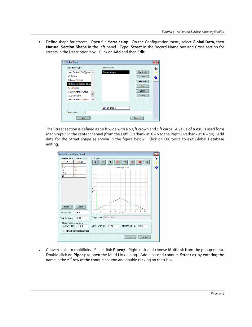
Tutorial 4 - Advanced Surface Water Hydraulics
1. Define shape for streets. Open file Yarra 42.xp. On the Configuration menu, select Global Data, then Natural Section Shape in the left panel. Type Street in the Record Name box and Cross section for streets in the Description box . Click on Add and then Edit.
The Street section is defined as 20 ft wide with a 0.3 ft crown and 1 ft curbs. A value of 0.016 is used form Manning’s n in the center channel (from the Left Overbank at X = 0 to the Right Overbank at X = 20). Add data for the Street shape as shown in the figure below. Click on OK twice to exit Global Database editing.
2. Convert links to multilinks. Select link Pipe07. Right click and choose Multilink from the popup menu. Double click on Pipe07 to open the Multi Link dialog. Add a second conduit, Street 07 by entering the name in the 2nd row of the conduit column and double clicking on the 2 box.
Page 4-13
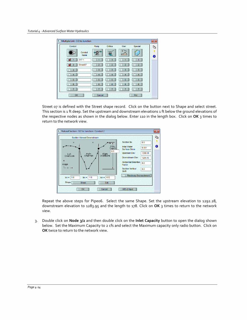
Tutorial 4 - Advanced Surface Water Hydraulics
Street 07 is defined with the Street shape record. Click on the button next to Shape and select street. This section is 1 ft deep. Set the upstream and downstream elevations 1 ft below the ground elevations of the respective nodes as shown in the dialog below. Enter 110 in the length box. Click on OK 3 times to return to the network view.
Repeat the above steps for Pipe06. Select the same Shape. Set the upstream elevation to 1292.28, downstream elevation to 1283.95 and the length to 178. Click on OK 3 times to return to the network view.
3. Double click on Node 3/2 and then double click on the Inlet Capacity button to open the dialog shown below. Set the Maximum Capacity to 2 cfs and select the Maximum capacity only radio button. Click on OK twice to return to the network view.
Page 4-14
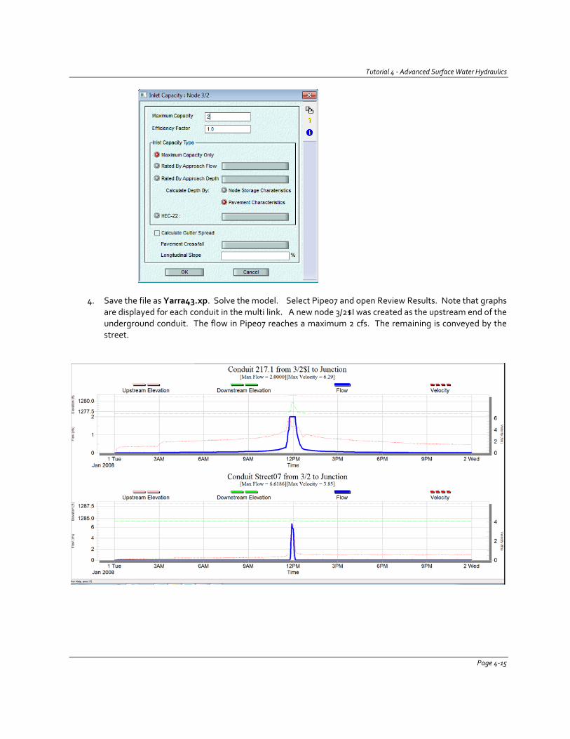
Tutorial 4 - Advanced Surface Water Hydraulics
4. Save the file as Yarra43.xp. Solve the model. Select Pipe07 and open Review Results. Note that graphs are displayed for each conduit in the multi link. A new node 3/2$I was created as the upstream end of the underground conduit. The flow in Pipe07 reaches a maximum 2 cfs. The remaining is conveyed by the street.
Page 4-15
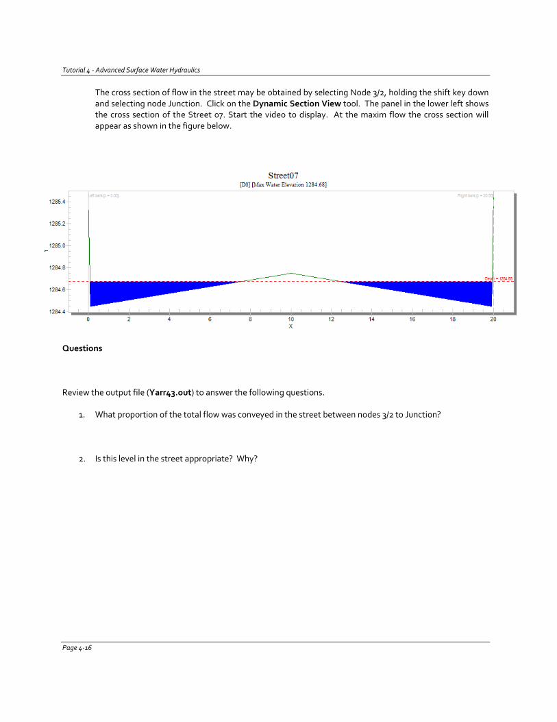
Tutorial 4 - Advanced Surface Water Hydraulics
The cross section of flow in the street may be obtained by selecting Node 3/2, holding the shift key down and selecting node Junction. Click on the Dynamic Section View tool. The panel in the lower left shows the cross section of the Street 07. Start the video to display. At the maxim flow the cross section will appear as shown in the figure below.
Questions
Review the output file (Yarr43.out) to answer the following questions.
1. What proportion of the total flow was conveyed in the street between nodes 3/2 to Junction?
2. Is this level in the street appropriate? Why?
Page 4-16
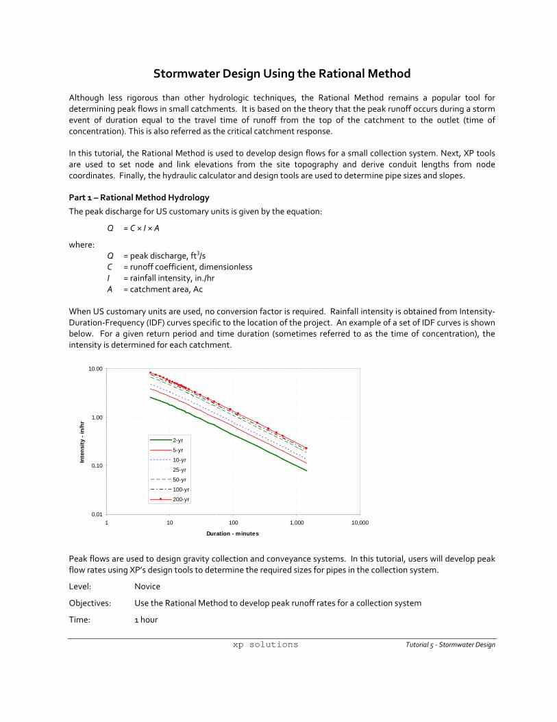
Stormwater Design Using the Rational Method
Although less rigorous than other hydrologic techniques, the Rational Method remains a popular tool for determining peak flows in small catchments. It is based on the theory that the peak runoff occurs during a storm event of duration equal to the travel time of runoff from the top of the catchment to the outlet (time of concentration). This is also referred as the critical catchment response.
In this tutorial, the Rational Method is used to develop design flows for a small collection system. Next, XP tools are used to set node and link elevations from the site topography and derive conduit lengths from node coordinates. Finally, the hydraulic calculator and design tools are used to determine pipe sizes and slopes.
Part 1 – Rational Method Hydrology
The peak discharge for US customary units is given by the equation:
Q = C × I × A
where: Q = peak discharge, ft3/s C = runoff coefficient, dimensionless I = rainfall intensity, in./hr A = catchment area, Ac When US customary units are used, no conversion factor is required. Rainfall intensity is obtained from Intensity-Duration-Frequency (IDF) curves specific to the location of the project. An example of a set of IDF curves is shown below. For a given return period and time duration (sometimes referred to as the time of concentration), the intensity is determined for each catchment.
Peak flows are used to design gravity collection and conveyance systems. In this tutorial, users will develop peak flow rates using XP’s design tools to determine the required sizes for pipes in the collection system.
Level: Novice
Objectives: Use the Rational Method to develop peak runoff rates for a collection system
Time: 1 hour
0.01
0.10
1.00
10.00
1 10 100 1,000 10,000
Duration - minutes
Inte
nsity
- in
/hr
2-yr
5-yr
10-yr
25-yr
50-yr
100-yr
200-yr
xp solutions Tutorial 5 - Stormwater Design
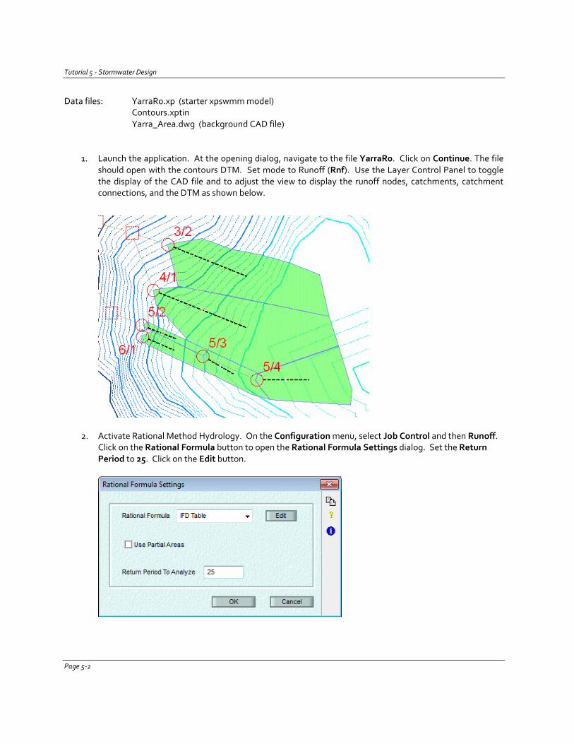
Tutorial 5 - Stormwater Design
Data files: YarraR0.xp (starter xpswmm model) Contours.xptin Yarra_Area.dwg (background CAD file)
1. Launch the application. At the opening dialog, navigate to the file YarraR0. Click on Continue. The file should open with the contours DTM. Set mode to Runoff (Rnf). Use the Layer Control Panel to toggle the display of the CAD file and to adjust the view to display the runoff nodes, catchments, catchment connections, and the DTM as shown below.
2. Activate Rational Method Hydrology. On the Configuration menu, select Job Control and then Runoff. Click on the Rational Formula button to open the Rational Formula Settings dialog. Set the Return Period to 25. Click on the Edit button.
Page 5-2
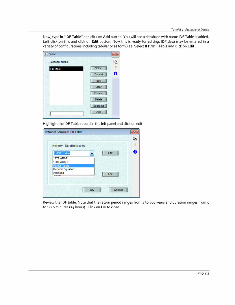
Tutorial 5 - Stormwater Design
Now, type in “IDF Table” and click on Add button. You will see a database with name IDF Table is added. Left click on this and click on Edit button. Now this is ready for editing. IDF data may be entered in a variety of configurations including tabular or as formulae. Select IFD/IDF Table and click on Edit.
Highlight the IDF Table record in the left panel and click on edit.
Review the IDF table. Note that the return period ranges from 2 to 200 years and duration ranges from 5 to 1440 minutes (24 hours). Click on OK to close.
Page 5-3
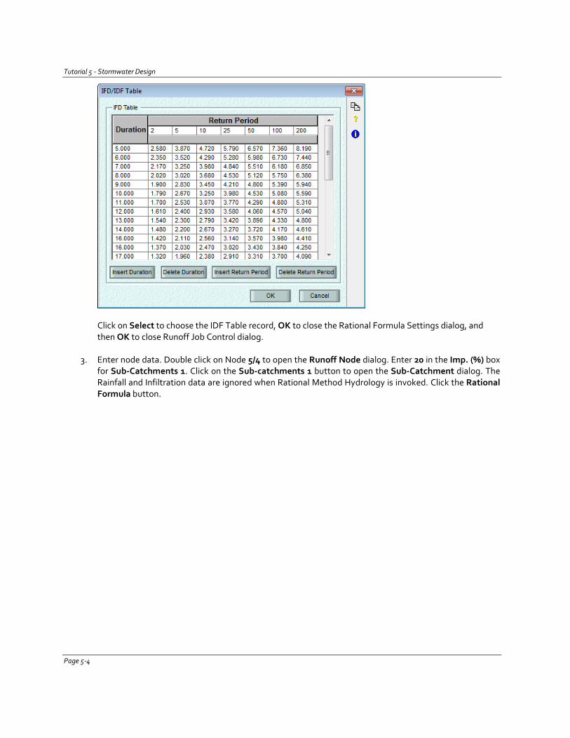
Tutorial 5 - Stormwater Design
Click on Select to choose the IDF Table record, OK to close the Rational Formula Settings dialog, and then OK to close Runoff Job Control dialog.
3. Enter node data. Double click on Node 5/4 to open the Runoff Node dialog. Enter 20 in the Imp. (%) box for Sub-Catchments 1. Click on the Sub-catchments 1 button to open the Sub-Catchment dialog. The Rainfall and Infiltration data are ignored when Rational Method Hydrology is invoked. Click the Rational Formula button.
Page 5-4
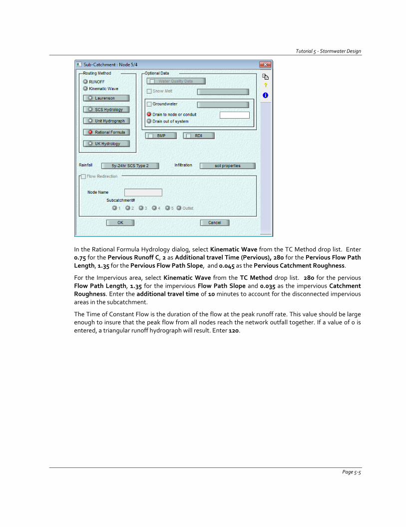
Tutorial 5 - Stormwater Design
In the Rational Formula Hydrology dialog, select Kinematic Wave from the TC Method drop list. Enter 0.75 for the Pervious Runoff C, 2 as Additional travel Time (Pervious), 280 for the Pervious Flow Path Length, 1.35 for the Pervious Flow Path Slope, and 0.045 as the Pervious Catchment Roughness.
For the Impervious area, select Kinematic Wave from the TC Method drop list. 280 for the pervious Flow Path Length, 1.35 for the impervious Flow Path Slope and 0.035 as the impervious Catchment Roughness. Enter the additional travel time of 10 minutes to account for the disconnected impervious areas in the subcatchment.
The Time of Constant Flow is the duration of the flow at the peak runoff rate. This value should be large enough to insure that the peak flow from all nodes reach the network outfall together. If a value of 0 is entered, a triangular runoff hydrograph will result. Enter 120.
Page 5-5
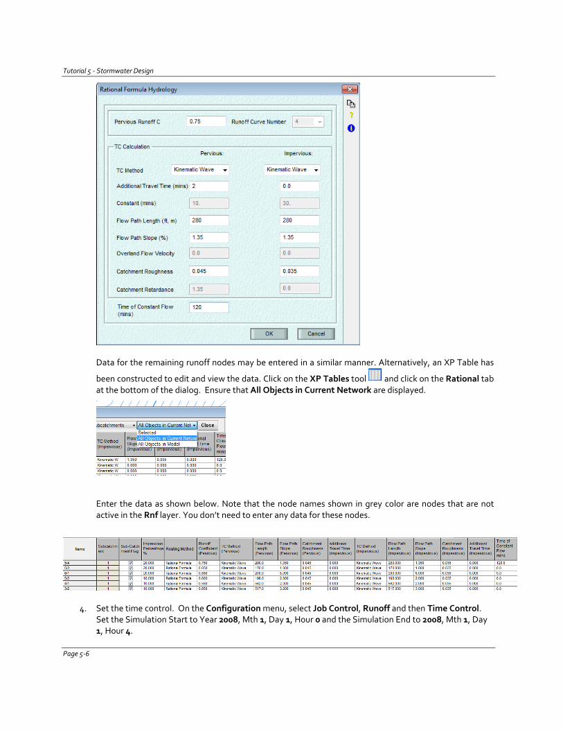
Tutorial 5 - Stormwater Design
Data for the remaining runoff nodes may be entered in a similar manner. Alternatively, an XP Table has
been constructed to edit and view the data. Click on the XP Tables tool and click on the Rational tab at the bottom of the dialog. Ensure that All Objects in Current Network are displayed.
Enter the data as shown below. Note that the node names shown in grey color are nodes that are not active in the Rnf layer. You don’t need to enter any data for these nodes.
4. Set the time control. On the Configuration menu, select Job Control, Runoff and then Time Control. Set the Simulation Start to Year 2008, Mth 1, Day 1, Hour 0 and the Simulation End to 2008, Mth 1, Day 1, Hour 4.
Page 5-6
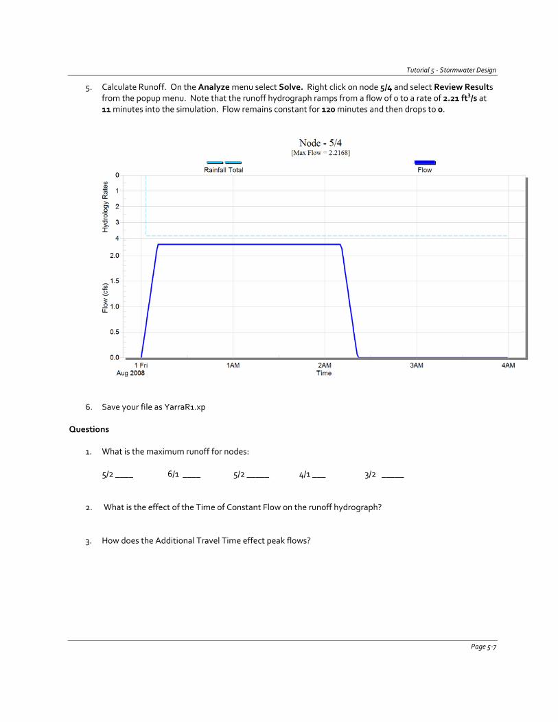
Tutorial 5 - Stormwater Design
5. Calculate Runoff. On the Analyze menu select Solve. Right click on node 5/4 and select Review Results from the popup menu. Note that the runoff hydrograph ramps from a flow of 0 to a rate of 2.21 ft3/s at 11 minutes into the simulation. Flow remains constant for 120 minutes and then drops to 0.
6. Save your file as YarraR1.xp
Questions
1. What is the maximum runoff for nodes: 5/2 ____ 6/1 ____ 5/2 _____ 4/1 ___ 3/2 _____ 2. What is the effect of the Time of Constant Flow on the runoff hydrograph?
3. How does the Additional Travel Time effect peak flows?
Page 5-7
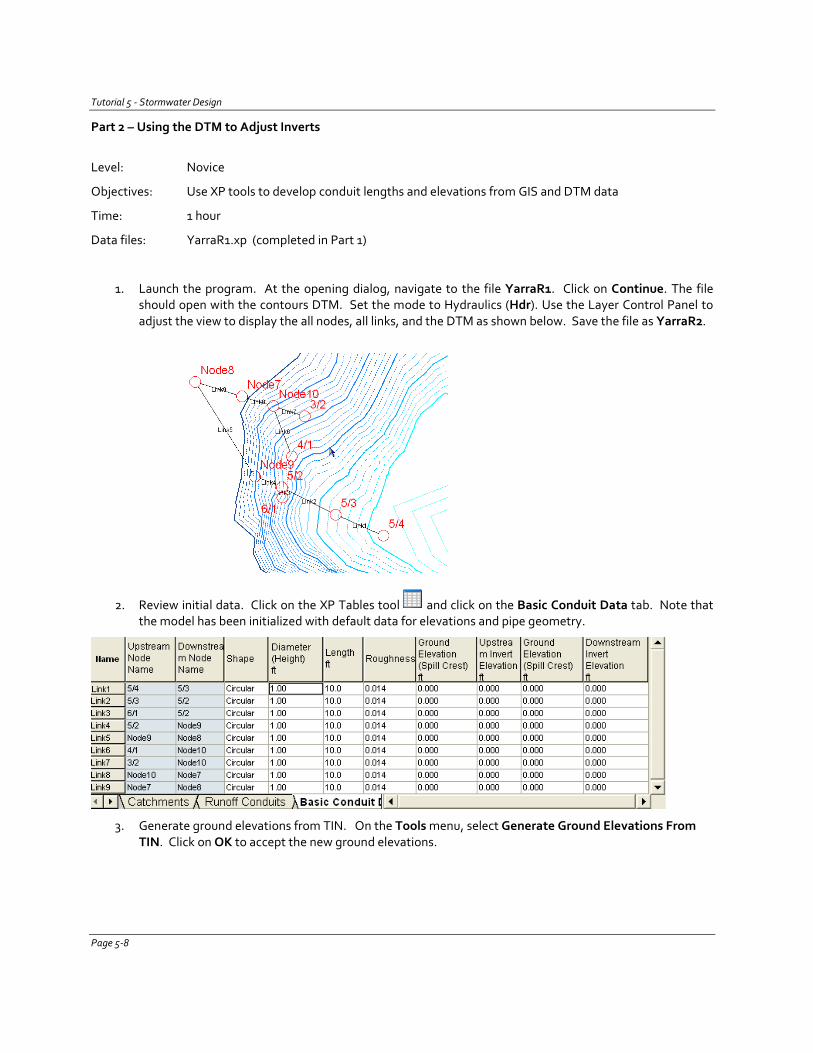
Tutorial 5 - Stormwater Design
Part 2 – Using the DTM to Adjust Inverts
Level: Novice
Objectives: Use XP tools to develop conduit lengths and elevations from GIS and DTM data
Time: 1 hour
Data files: YarraR1.xp (completed in Part 1)
1. Launch the program. At the opening dialog, navigate to the file YarraR1. Click on Continue. The file should open with the contours DTM. Set the mode to Hydraulics (Hdr). Use the Layer Control Panel to adjust the view to display the all nodes, all links, and the DTM as shown below. Save the file as YarraR2.
2. Review initial data. Click on the XP Tables tool and click on the Basic Conduit Data tab. Note that the model has been initialized with default data for elevations and pipe geometry.
3. Generate ground elevations from TIN. On the Tools menu, select Generate Ground Elevations From TIN. Click on OK to accept the new ground elevations.
Page 5-8
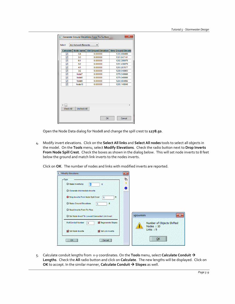
Tutorial 5 - Stormwater Design
Open the Node Data dialog for Node8 and change the spill crest to 1278.50.
4. Modify invert elevations. Click on the Select All links and Select All nodes tools to select all objects in
the model. On the Tools menu, select Modify Elevations. Check the radio button next to Drop Inverts From Node Spill Crest. Check the boxes as shown in the dialog below. This will set node inverts to 8 feet below the ground and match link inverts to the nodes inverts.
Click on OK. The number of nodes and links with modified inverts are reported.
5. Calculate conduit lengths from x-y coordinates. On the Tools menu, select Calculate Conduit
Lengths. Check the All radio button and click on Calculate. The new lengths will be displayed. Click on OK to accept. In the similar manner, Calculate Conduit Slopes as well.
Page 5-9
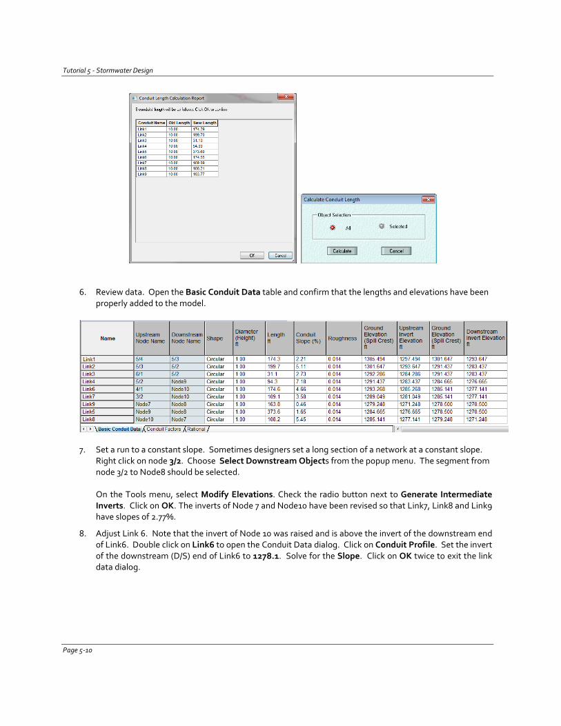
Tutorial 5 - Stormwater Design
6. Review data. Open the Basic Conduit Data table and confirm that the lengths and elevations have been properly added to the model.
7. Set a run to a constant slope. Sometimes designers set a long section of a network at a constant slope.
Right click on node 3/2. Choose Select Downstream Objects from the popup menu. The segment from node 3/2 to Node8 should be selected.
On the Tools menu, select Modify Elevations. Check the radio button next to Generate Intermediate Inverts. Click on OK. The inverts of Node 7 and Node10 have been revised so that Link7, Link8 and Link9 have slopes of 2.77%.
8. Adjust Link 6. Note that the invert of Node 10 was raised and is above the invert of the downstream end of Link6. Double click on Link6 to open the Conduit Data dialog. Click on Conduit Profile. Set the invert of the downstream (D/S) end of Link6 to 1278.1. Solve for the Slope. Click on OK twice to exit the link data dialog.
Page 5-10
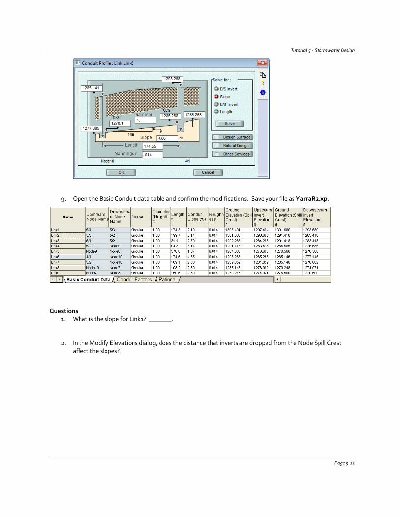
Tutorial 5 - Stormwater Design
9. Open the Basic Conduit data table and confirm the modifications. Save your file as YarraR2.xp.
Questions
1. What is the slope for Link1? _______.
2. In the Modify Elevations dialog, does the distance that inverts are dropped from the Node Spill Crest
affect the slopes?
Page 5-11
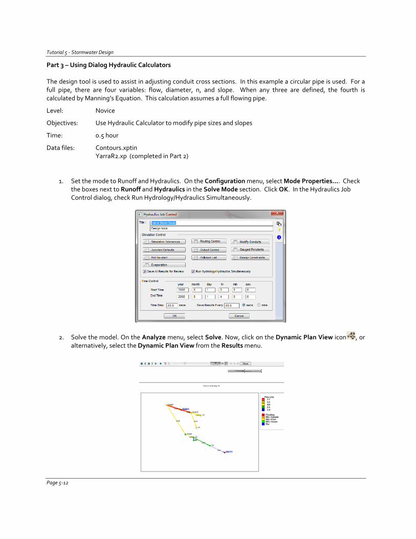
Tutorial 5 - Stormwater Design
Part 3 – Using Dialog Hydraulic Calculators The design tool is used to assist in adjusting conduit cross sections. In this example a circular pipe is used. For a full pipe, there are four variables: flow, diameter, n, and slope. When any three are defined, the fourth is calculated by Manning’s Equation. This calculation assumes a full flowing pipe.
Level: Novice
Objectives: Use Hydraulic Calculator to modify pipe sizes and slopes
Time: 0.5 hour
Data files: Contours.xptin YarraR2.xp (completed in Part 2)
1. Set the mode to Runoff and Hydraulics. On the Configuration menu, select Mode Properties…. Check the boxes next to Runoff and Hydraulics in the Solve Mode section. Click OK. In the Hydraulics Job Control dialog, check Run Hydrology/Hydraulics Simultaneously.
2. Solve the model. On the Analyze menu, select Solve. Now, click on the Dynamic Plan View icon , or alternatively, select the Dynamic Plan View from the Results menu.
Page 5-12
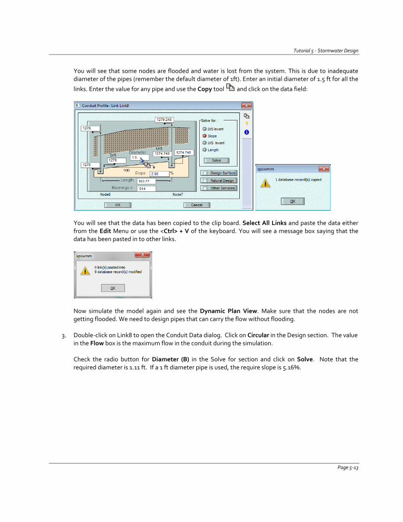
Tutorial 5 - Stormwater Design
You will see that some nodes are flooded and water is lost from the system. This is due to inadequate diameter of the pipes (remember the default diameter of 1ft). Enter an initial diameter of 1.5 ft for all the
links. Enter the value for any pipe and use the Copy tool and click on the data field:
You will see that the data has been copied to the clip board. Select All Links and paste the data either from the Edit Menu or use the <Ctrl> + V of the keyboard. You will see a message box saying that the data has been pasted in to other links.
Now simulate the model again and see the Dynamic Plan View. Make sure that the nodes are not getting flooded. We need to design pipes that can carry the flow without flooding.
3. Double-click on Link8 to open the Conduit Data dialog. Click on Circular in the Design section. The value
in the Flow box is the maximum flow in the conduit during the simulation.
Check the radio button for Diameter (B) in the Solve for section and click on Solve. Note that the required diameter is 1.11 ft. If a 1 ft diameter pipe is used, the require slope is 5.16%.
Page 5-13
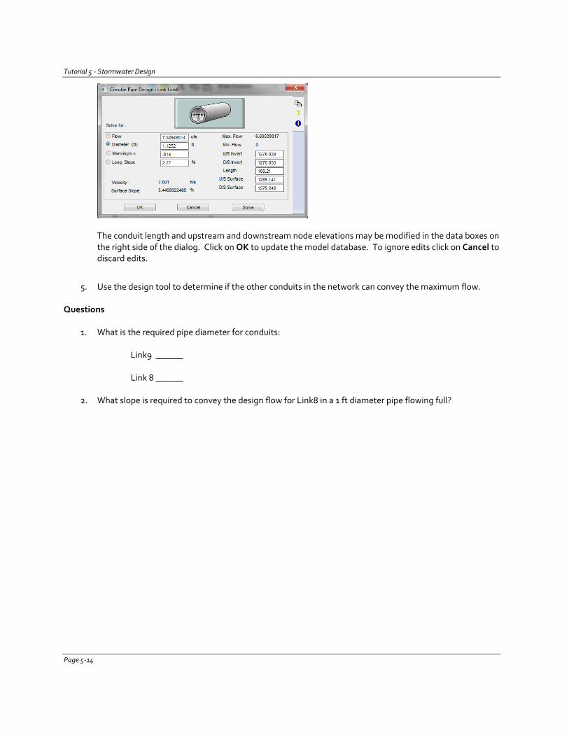
Tutorial 5 - Stormwater Design
The conduit length and upstream and downstream node elevations may be modified in the data boxes on the right side of the dialog. Click on OK to update the model database. To ignore edits click on Cancel to discard edits.
5. Use the design tool to determine if the other conduits in the network can convey the maximum flow.
Questions
1. What is the required pipe diameter for conduits: Link9 ______ Link 8 ______
2. What slope is required to convey the design flow for Link8 in a 1 ft diameter pipe flowing full?
Page 5-14
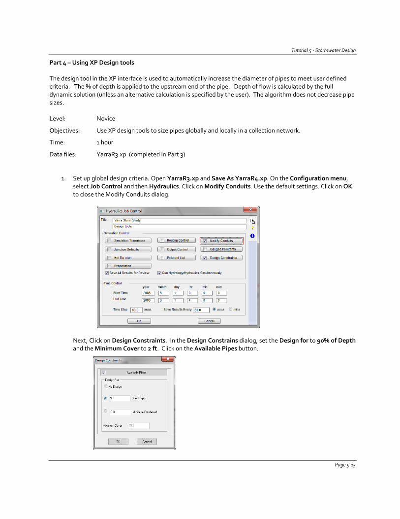
Tutorial 5 - Stormwater Design
Part 4 – Using XP Design tools The design tool in the XP interface is used to automatically increase the diameter of pipes to meet user defined criteria. The % of depth is applied to the upstream end of the pipe. Depth of flow is calculated by the full dynamic solution (unless an alternative calculation is specified by the user). The algorithm does not decrease pipe sizes. Level: Novice
Objectives: Use XP design tools to size pipes globally and locally in a collection network.
Time: 1 hour
Data files: YarraR3.xp (completed in Part 3)
1. Set up global design criteria. Open YarraR3.xp and Save As YarraR4.xp. On the Configuration menu, select Job Control and then Hydraulics. Click on Modify Conduits. Use the default settings. Click on OK to close the Modify Conduits dialog.
Next, Click on Design Constraints. In the Design Constrains dialog, set the Design for to 90% of Depth and the Minimum Cover to 2 ft. Click on the Available Pipes button.
Page 5-15
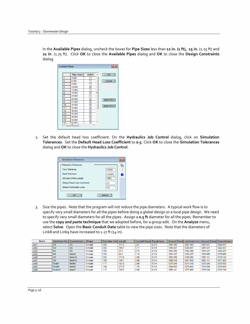
Tutorial 5 - Stormwater Design
In the Available Pipes dialog, uncheck the boxes for Pipe Sizes less than 12 in. (1 ft), 15 in. (1.25 ft) and 21 in. (1.75 ft). Click OK to close the Available Pipes dialog and OK to close the Design Constraints dialog.
2. Set the default head loss coefficient. On the Hydraulics Job Control dialog, click on Simulation Tolerances. Set the Default Head Loss Coefficient to 0.5. Click OK to close the Simulation Tolerances dialog and OK to close the Hydraulics Job Control.
3. Size the pipes. Note that the program will not reduce the pipe diameters. A typical work flow is to specify very small diameters for all the pipes before doing a global design or a local pipe design. We need to specify very small diameters for all the pipes. Assign a 0.5 ft diameter for all the pipes. Remember to use the copy and paste technique that we adopted before, for a group edit. On the Analyze menu, select Solve. Open the Basic Conduit Data table to view the pipe sizes. Note that the diameters of Link8 and Link9 have increased to 1.17 ft (14 in).
Page 5-16
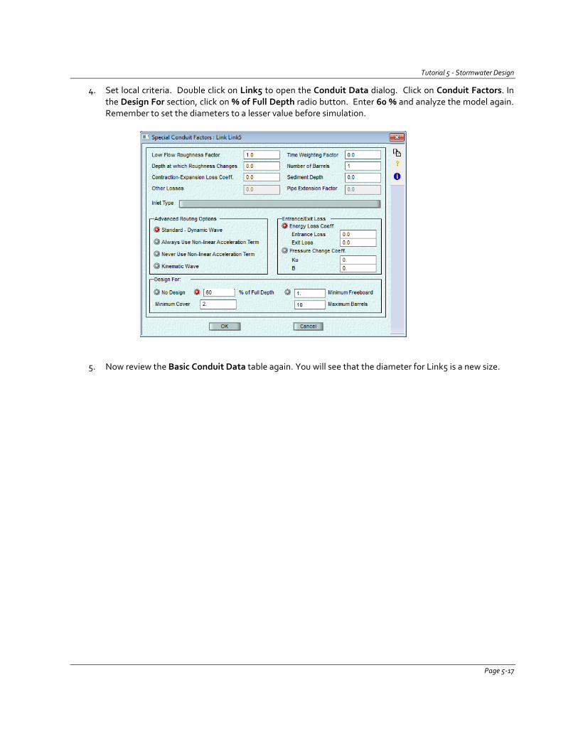
Tutorial 5 - Stormwater Design
4. Set local criteria. Double click on Link5 to open the Conduit Data dialog. Click on Conduit Factors. In the Design For section, click on % of Full Depth radio button. Enter 60 % and analyze the model again. Remember to set the diameters to a lesser value before simulation.
5. Now review the Basic Conduit Data table again. You will see that the diameter for Link5 is a new size.
Page 5-17

Tutorial 5 - Stormwater Design
Questions
1. Does the addition of a tailwater condition to the outfall require a larger pipe diameter for link9? Why or why not?
2. Determine the required pipe diameters to convey the 100-yr storm with the design constraints described in Step 1.
Page 5-18
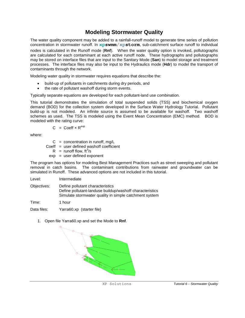
Modeling Stormwater Quality The water quality component may be added to a rainfall-runoff model to generate time series of pollution concentration in stormwater runoff. In xpswmm/xpstorm, sub-catchment surface runoff to individual nodes is calculated in the Runoff mode (Rnf). When the water quality option is invoked, pollutographs are calculated for each contaminant at each active runoff node. These hydrographs and pollutographs may be stored on interface files that are input to the Sanitary Mode (San) to model storage and treatment processes. The interface files may also be input to the Hydraulics mode (Hdr) to model the transport of contaminants through the network.
Modeling water quality in stormwater requires equations that describe the:
• build-up of pollutants in catchments during dry periods, and • the rate of pollutant washoff during storm events.
Typically separate equations are developed for each pollutant-land use combination.
This tutorial demonstrates the simulation of total suspended solids (TSS) and biochemical oxygen demand (BOD) for the collection system developed in the Surface Water Hydrology Tutorial. Pollutant build-up is not modeled. An infinite source is assumed to be available for washoff. Two washoff schemes as used. The TSS is modeled using the Event Mean Concentration (EMC) method. BOD is modeled with the rating curve:
C = Coeff × Rexp
where:
C = concentration in runoff, mg/L Coeff = user defined washoff coefficient R = runoff flow, ft3/s exp = user defined exponent
The program has options for modeling Best Management Practices such as street sweeping and pollutant removal in catch basins. The contaminant contributions from rainwater and groundwater can be simulated in Runoff. These advanced options are not included in this tutorial.
Level: Intermediate
Objectives: Define pollutant characteristics Define pollutant-landuse buildup/washoff characteristics Simulate stormwater quality in simple catchment system
Time: 1 hour
Data files: Yarra60.xp (starter file)
1. Open file Yarra60.xp and set the Mode to Rnf.
XP Solutions Tutorial 6 – Stormwater Quality
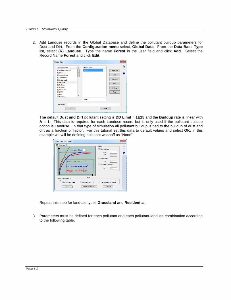
Tutorial 6 – Stormwater Quality
2. Add Landuse records in the Global Database and define the pollutant buildup parameters for Dust and Dirt. From the Configuration menu select, Global Data. From the Data Base Type list, select (R) Landuse. Type the name Forest in the user field and click Add. Select the Record Name Forest and click Edit.
The default Dust and Dirt pollutant setting is DD Limit = 1E25 and the Buildup rate is linear with A = 1. This data is required for each Landuse record but is only used if the pollutant buildup option is Landuse. In that type of simulation all pollutant buildup is tied to the buildup of dust and dirt as a fraction or factor. For this tutorial set this data to default values and select OK. In this example we will be defining pollutant washoff as “None”.
Repeat this step for landuse types Grassland and Residential.
3. Parameters must be defined for each pollutant and each pollutant-landuse combination according to the following table.
Page 6-2
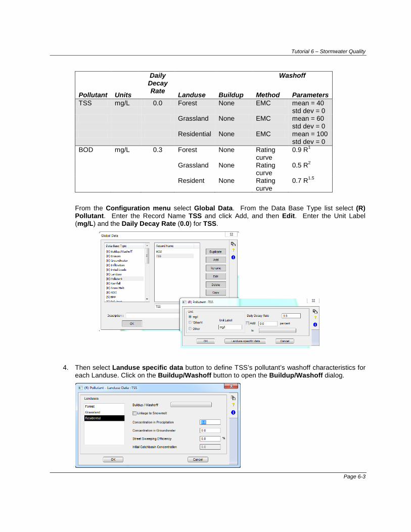
Tutorial 6 – Stormwater Quality
Daily Decay Rate
Washoff
Pollutant Units Landuse Buildup Method Parameters TSS mg/L 0.0 Forest None EMC mean = 40
std dev = 0 Grassland None EMC mean = 60
std dev = 0 Residential None EMC mean = 100
std dev = 0 BOD mg/L 0.3 Forest None Rating
curve 0.9 R1
Grassland None Rating curve
0.5 R2
Resident None Rating curve
0.7 R1.5
From the Configuration menu select Global Data. From the Data Base Type list select (R) Pollutant. Enter the Record Name TSS and click Add, and then Edit. Enter the Unit Label (mg/L) and the Daily Decay Rate (0.0) for TSS.
4. Then select Landuse specific data button to define TSS’s pollutant’s washoff characteristics for each Landuse. Click on the Buildup/Washoff button to open the Buildup/Washoff dialog.
Page 6-3
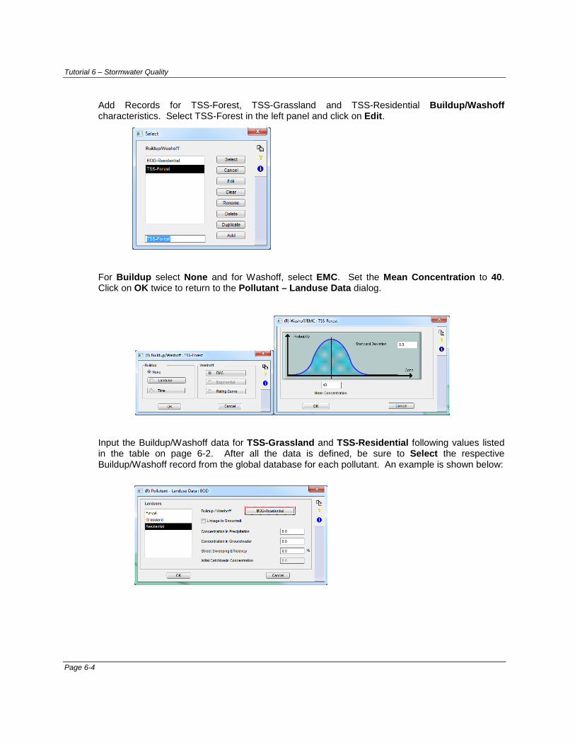
Tutorial 6 – Stormwater Quality
Add Records for TSS-Forest, TSS-Grassland and TSS-Residential Buildup/Washoff characteristics. Select TSS-Forest in the left panel and click on Edit.
For Buildup select None and for Washoff, select EMC. Set the Mean Concentration to 40. Click on OK twice to return to the Pollutant – Landuse Data dialog.
Input the Buildup/Washoff data for TSS-Grassland and TSS-Residential following values listed in the table on page 6-2. After all the data is defined, be sure to Select the respective Buildup/Washoff record from the global database for each pollutant. An example is shown below:
Page 6-4
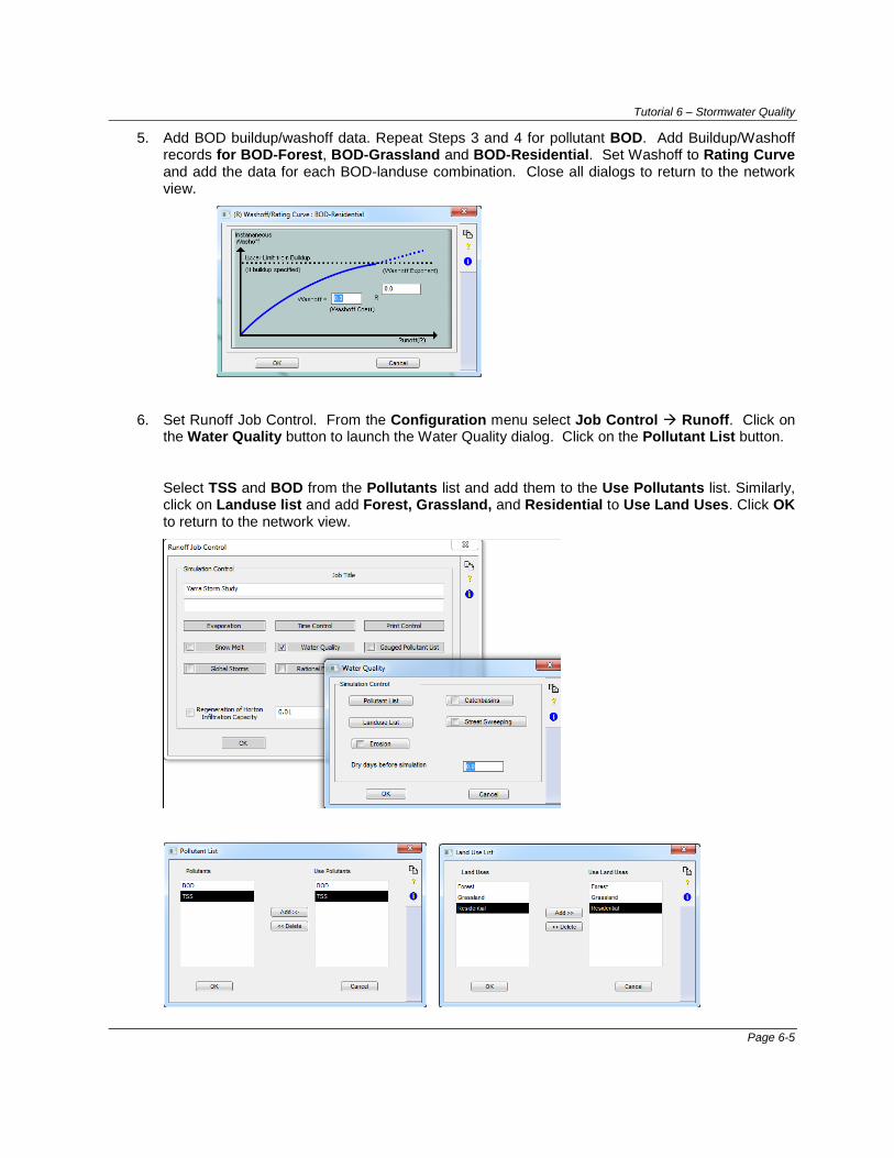
Tutorial 6 – Stormwater Quality
5. Add BOD buildup/washoff data. Repeat Steps 3 and 4 for pollutant BOD. Add Buildup/Washoff records for BOD-Forest, BOD-Grassland and BOD-Residential. Set Washoff to Rating Curve and add the data for each BOD-landuse combination. Close all dialogs to return to the network view.
6. Set Runoff Job Control. From the Configuration menu select Job Control Runoff. Click on the Water Quality button to launch the Water Quality dialog. Click on the Pollutant List button.
Select TSS and BOD from the Pollutants list and add them to the Use Pollutants list. Similarly, click on Landuse list and add Forest, Grassland, and Residential to Use Land Uses. Click OK to return to the network view.
Page 6-5
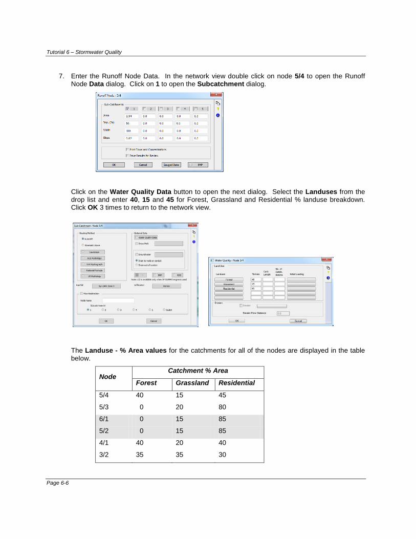
Tutorial 6 – Stormwater Quality
7. Enter the Runoff Node Data. In the network view double click on node 5/4 to open the Runoff Node Data dialog. Click on 1 to open the Subcatchment dialog.
Click on the Water Quality Data button to open the next dialog. Select the Landuses from the drop list and enter 40, 15 and 45 for Forest, Grassland and Residential % landuse breakdown. Click OK 3 times to return to the network view.
The Landuse - % Area values for the catchments for all of the nodes are displayed in the table below.
Node Catchment % Area
Forest Grassland Residential
5/4 40 15 45
5/3 0 20 80
6/1 0 15 85
5/2 0 15 85
4/1 40 20 40
3/2 35 35 30
Page 6-6
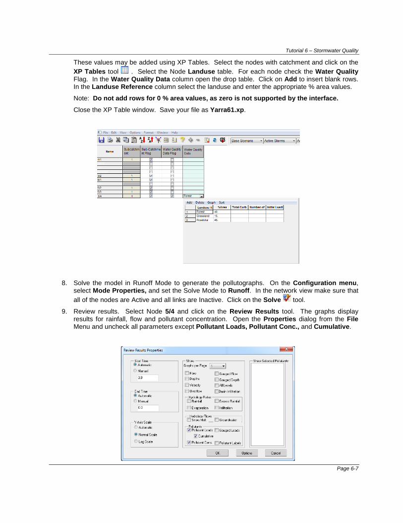
Tutorial 6 – Stormwater Quality
These values may be added using XP Tables. Select the nodes with catchment and click on the XP Tables tool . Select the Node Landuse table. For each node check the Water Quality Flag. In the Water Quality Data column open the drop table. Click on Add to insert blank rows. In the Landuse Reference column select the landuse and enter the appropriate % area values.
Note: Do not add rows for 0 % area values, as zero is not supported by the interface.
Close the XP Table window. Save your file as Yarra61.xp.
8. Solve the model in Runoff Mode to generate the pollutographs. On the Configuration menu, select Mode Properties, and set the Solve Mode to Runoff. In the network view make sure that all of the nodes are Active and all links are Inactive. Click on the Solve tool.
9. Review results. Select Node 5/4 and click on the Review Results tool. The graphs display results for rainfall, flow and pollutant concentration. Open the Properties dialog from the File Menu and uncheck all parameters except Pollutant Loads, Pollutant Conc., and Cumulative.
Page 6-7

Tutorial 6 – Stormwater Quality
The graph displays time series of Cumulative Load (lbs) and Concentration (mg/L) for TSS and BOD. Note that the TSS concentration is constant during the simulation.
Questions
1. What is the maximum is the concentration of BOD in runoff from Node 4/1?
2. Review Table R9 in the output file to determine the total loads of :
a. TSS? _____ lb
b. BOD? _____ lb
Page 6-8
Sanitary Sewer Modeling xp models are used to simulate the hydraulics in sanitary and combined sewer systems. Models account for gravity flow in open or closed top conduits, storage in wet wells, pumps, and flow in force mains. Networks may be looped or have multiple outfalls.
Numerous tools are used to develop constant and time series flows and unit rated flows. Diurnal and weekly variation patterns may be assigned to any flow. Infiltration and wet weather flows are described in Tutorial 8. Water quality routing and treatment are described in Tutorial 9.
Most sanitary utility managers make use of some form of asset management or GIS software to manage collection system data. The program has a variety of tools to import such data as background images, GIS layers or directly as objects in the model. The data used for this exercise has been received from a GIS department and was edited or appended to add additional information. Also, there are some instances where additional information may be needed (e.g. conduit shapes, Manning’s n, etc.).
ESRI shapefile, MapInfo MID/MIF, Autodesk DWG/DXF files and georeferenced photographs with extensions of *.ECW, *.SID, *.JPG, *.TIF, *.BMP and others may be added to models as background images. When shapefiles are incorporated as background images, the display can be color coded by attribute value.
In Part 1 of this tutorial, users will build a sanitary sewer collection system model by importing data from external databases. Fields in the xp model will be filled by data from *.dbf, *.shp, and *.xpx files. In Part 2, a Digital Terrain Model (DTM) will be constructed using the manhole (pit) ground elevations.
Part 1 – Building a Sanitary Sewer Model from External Data
A collection network can be developed in the graphical user interface using a variety of methods. In Part 1, users will learn how to utilize xp’s tools to import GIS and database files to develop a pipe network including dry weather flow data, node data, and conduit data. Global data is added using XPX files. Level: Novice
Objectives: Introduce the steps required to: • Build a sanitary sewer model using external data • Load images using Shape files as the background • Digitize a network importing all node and conduit data
Time: 2 hours
Data files: The model will be developed from data contained in the files listed in Table 1.
Table 1 – External data files used to build sanitary sewer model
File Name Extensions Description Cadastre .dbf, .prj,.shp., shx Background image containing property
boundaries SanNodes .dbf, .prj, .shp, .shx Node data SanCond .dbf, .prj, .shp, .shx Link data SanFlow .dbf, .prj, .shp, .shx Sanitary flows SanPump .dbf, .prj, .shp, .shx Pump data DWF .xpx Dry weather Flow pattern PC .xpx Pump Rating curve
XP Solutions Tutorial 7 - Sanitary Sewer Modeling
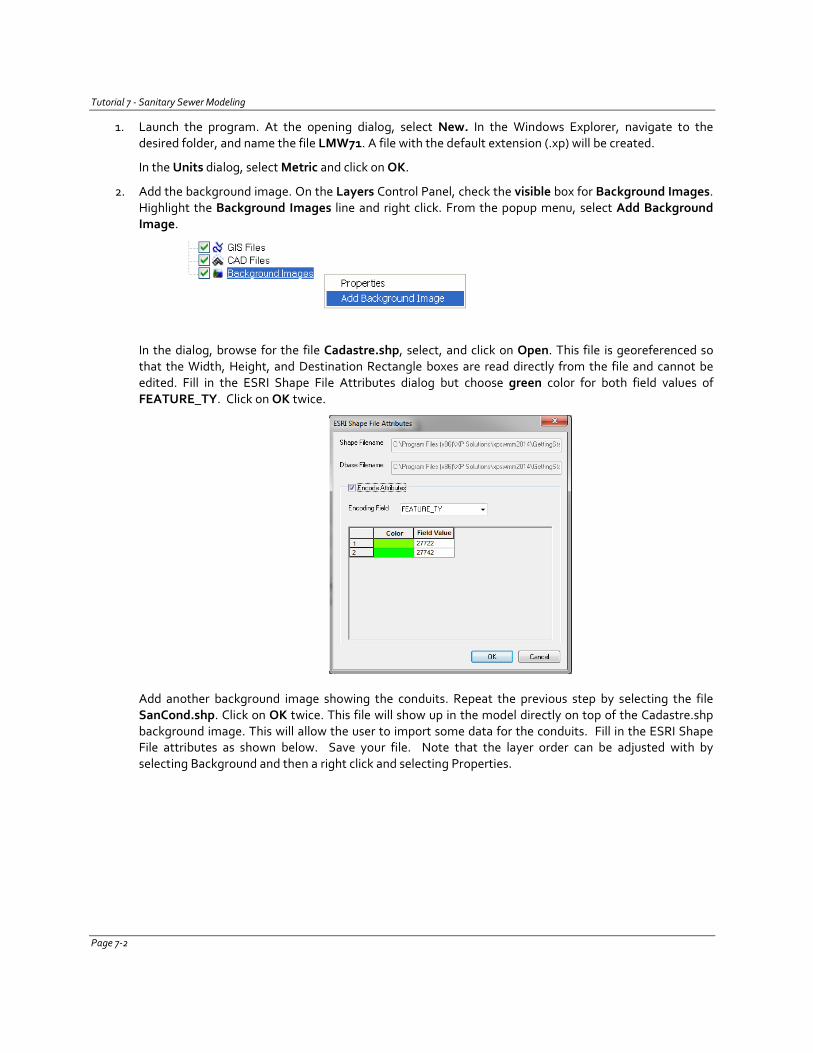
Tutorial 7 - Sanitary Sewer Modeling
1. Launch the program. At the opening dialog, select New. In the Windows Explorer, navigate to the desired folder, and name the file LMW71. A file with the default extension (.xp) will be created.
In the Units dialog, select Metric and click on OK.
2. Add the background image. On the Layers Control Panel, check the visible box for Background Images. Highlight the Background Images line and right click. From the popup menu, select Add Background Image.
In the dialog, browse for the file Cadastre.shp, select, and click on Open. This file is georeferenced so that the Width, Height, and Destination Rectangle boxes are read directly from the file and cannot be edited. Fill in the ESRI Shape File Attributes dialog but choose green color for both field values of FEATURE_TY. Click on OK twice.
Add another background image showing the conduits. Repeat the previous step by selecting the file SanCond.shp. Click on OK twice. This file will show up in the model directly on top of the Cadastre.shp background image. This will allow the user to import some data for the conduits. Fill in the ESRI Shape File attributes as shown below. Save your file. Note that the layer order can be adjusted with by selecting Background and then a right click and selecting Properties.
Page 7-2
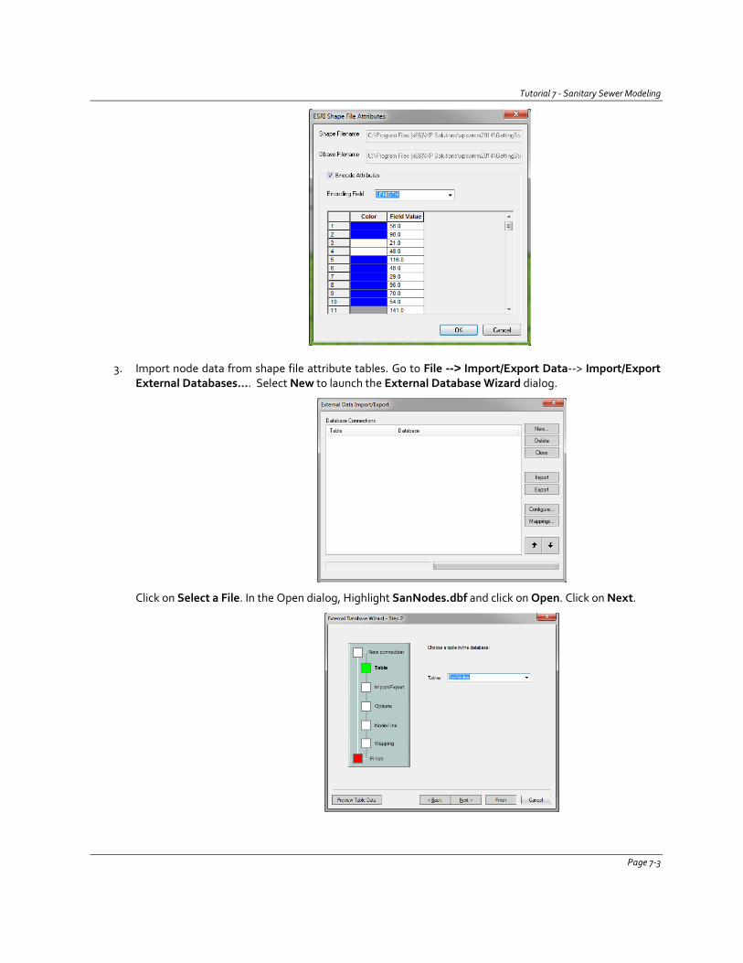
Tutorial 7 - Sanitary Sewer Modeling
3. Import node data from shape file attribute tables. Go to File --> Import/Export Data--> Import/Export External Databases…. Select New to launch the External Database Wizard dialog.
Click on Select a File. In the Open dialog, Highlight SanNodes.dbf and click on Open. Click on Next.
Page 7-3

Tutorial 7 - Sanitary Sewer Modeling
In Wizard Step 2, ensure that SanNodes is showing in the Tables dropdown menu. Select Next.
In Wizard Step 3, select Import Data Only and select Next.
In Wizard Step 4, select Create New or Update Existing from the drop list. Click on Next.
In Wizard Step 5, fill in text as shown. Click on Preview Table to check the data in the table. Click on Next.
Page 7-4
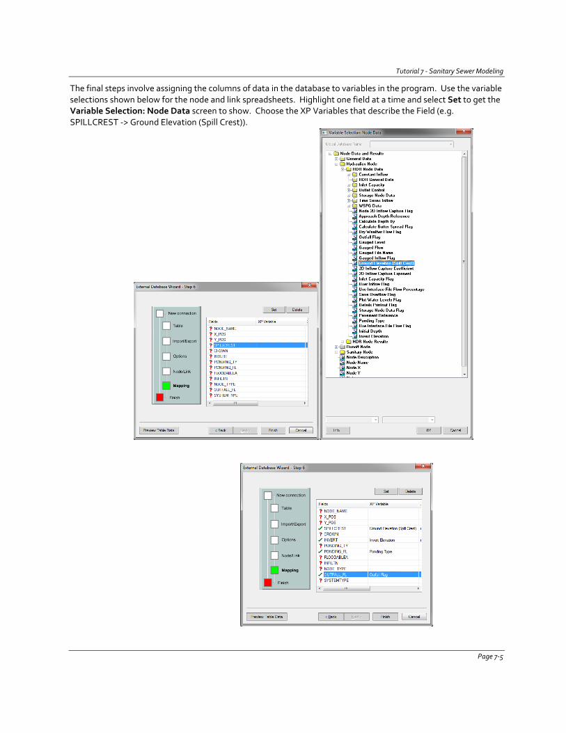
Tutorial 7 - Sanitary Sewer Modeling
The final steps involve assigning the columns of data in the database to variables in the program. Use the variable selections shown below for the node and link spreadsheets. Highlight one field at a time and select Set to get the Variable Selection: Node Data screen to show. Choose the XP Variables that describe the Field (e.g. SPILLCREST -> Ground Elevation (Spill Crest)).
Page 7-5
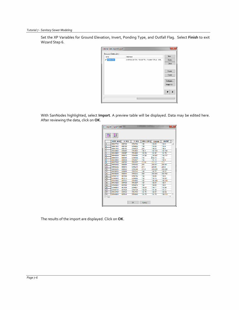
Tutorial 7 - Sanitary Sewer Modeling
Set the XP Variables for Ground Elevation, Invert, Ponding Type, and Outfall Flag. Select Finish to exit Wizard Step 6.
With SanNodes highlighted, select Import. A preview table will be displayed. Data may be edited here. After reviewing the data, click on OK.
The results of the import are displayed. Click on OK.
Page 7-6
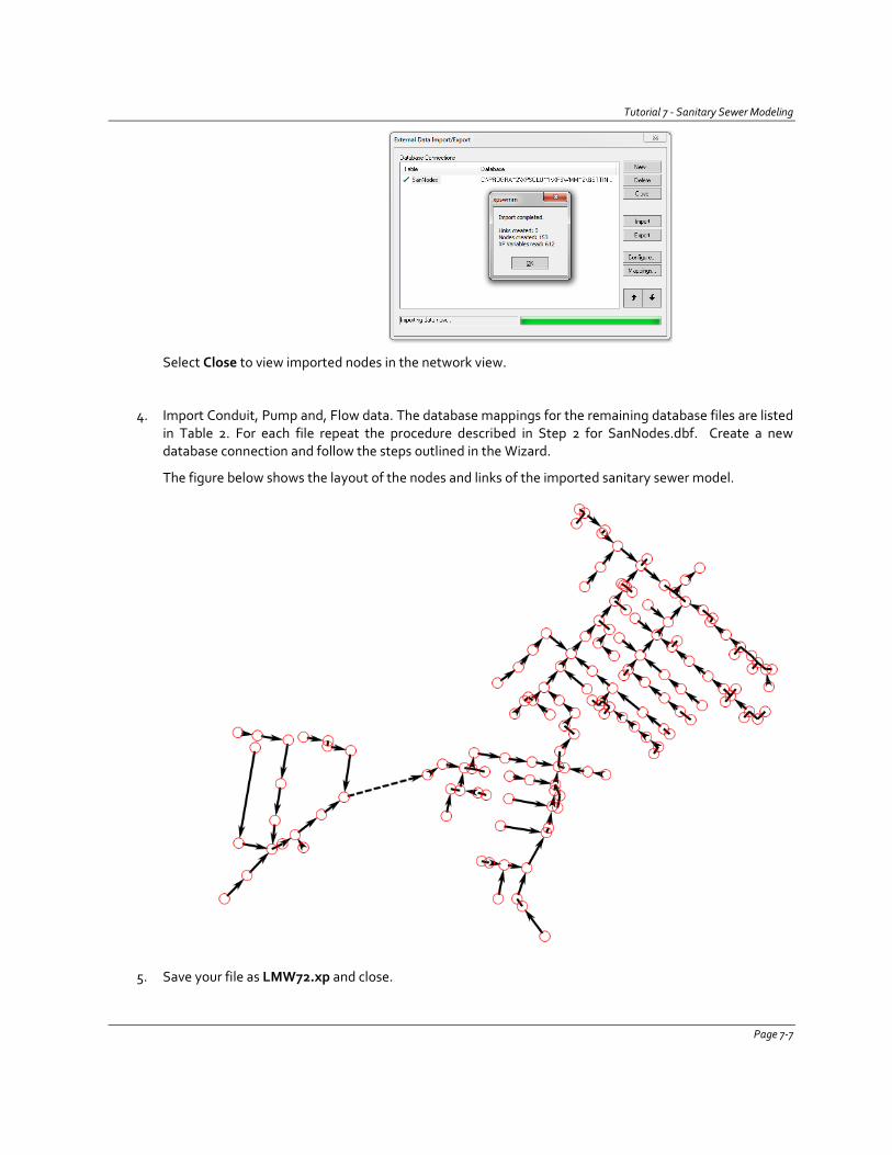
Tutorial 7 - Sanitary Sewer Modeling
Select Close to view imported nodes in the network view.
4. Import Conduit, Pump and, Flow data. The database mappings for the remaining database files are listed in Table 2. For each file repeat the procedure described in Step 2 for SanNodes.dbf. Create a new database connection and follow the steps outlined in the Wizard.
The figure below shows the layout of the nodes and links of the imported sanitary sewer model.
5. Save your file as LMW72.xp and close.
Page 7-7
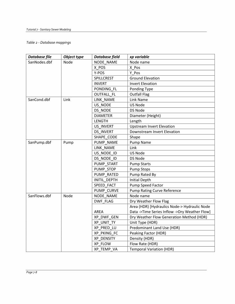
Tutorial 7 - Sanitary Sewer Modeling
Table 2 - Database mappings
Database file Object type Database field xp variable SanNodes.dbf Node NODE_NAME Node name
X_POS X_Pos Y-POS Y_Pos SPILLCREST Ground Elevation INVERT Invert Elevation PONDING_FL Ponding Type OUTFALL_FL Outfall Flag
SanCond.dbf Link LINK_NAME Link Name US_NODE US Node DS_NODE DS Node DIAMETER Diameter (Height) LENGTH Length US_INVERT Upstream Invert Elevation DS_INVERT Downstream Invert Elevation SHAPE_CODE Shape
SanPump.dbf Pump PUMP_NAME Pump Name LINK_NAME Link US_NODE_ID US Node DS_NODE_ID DS Node PUMP_START Pump Starts PUMP_STOP Pump Stops PUMP_RATED Pump Rated By INITIL_DEPTH Initial Depth SPEED_FACT Pump Speed Factor PUMP_CURVE Pump Rating Curve Reference
SanFlows.dbf Node NODE_NAME Node name DWF_FLAG Dry Weather Flow Flag
AREA Area (HDR) [Hydraulics Node-> Hydraulic Node Data ->Time Series Inflow ->Dry Weather Flow]
XP_DWF_GEN Dry Weather Flow Generation Method (HDR) XP_UNIT_TY Unit Type (HDR) XP_PRED_LU Predominant Land Use (HDR) XP_PKING_FC Peaking Factor (HDR) XP_DENSITY Density (HDR) XP_FLOW Flow Rate (HDR) XP_TEMP_VA Temporal Variation (HDR)
Page 7-8
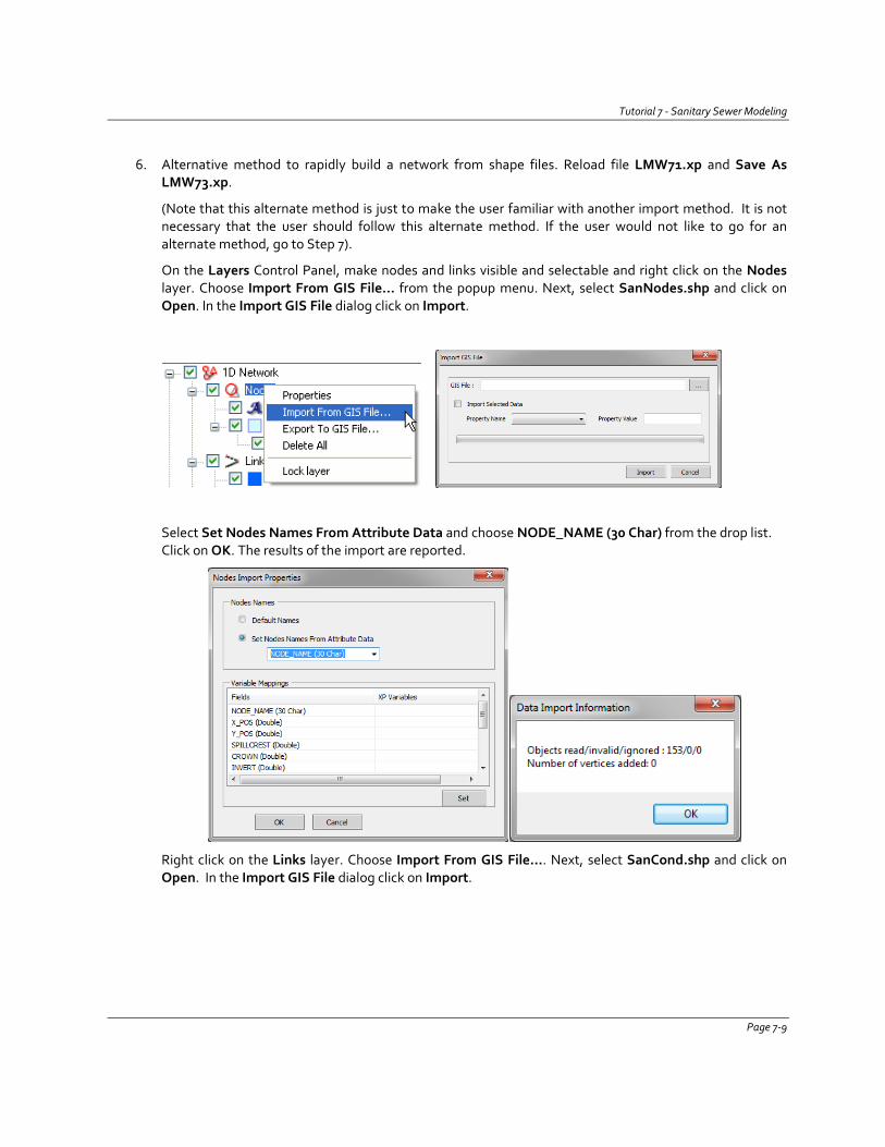
Tutorial 7 - Sanitary Sewer Modeling
6. Alternative method to rapidly build a network from shape files. Reload file LMW71.xp and Save As LMW73.xp.
(Note that this alternate method is just to make the user familiar with another import method. It is not necessary that the user should follow this alternate method. If the user would not like to go for an alternate method, go to Step 7).
On the Layers Control Panel, make nodes and links visible and selectable and right click on the Nodes layer. Choose Import From GIS File… from the popup menu. Next, select SanNodes.shp and click on Open. In the Import GIS File dialog click on Import.
Select Set Nodes Names From Attribute Data and choose NODE_NAME (30 Char) from the drop list. Click on OK. The results of the import are reported.
Right click on the Links layer. Choose Import From GIS File…. Next, select SanCond.shp and click on Open. In the Import GIS File dialog click on Import.
Page 7-9
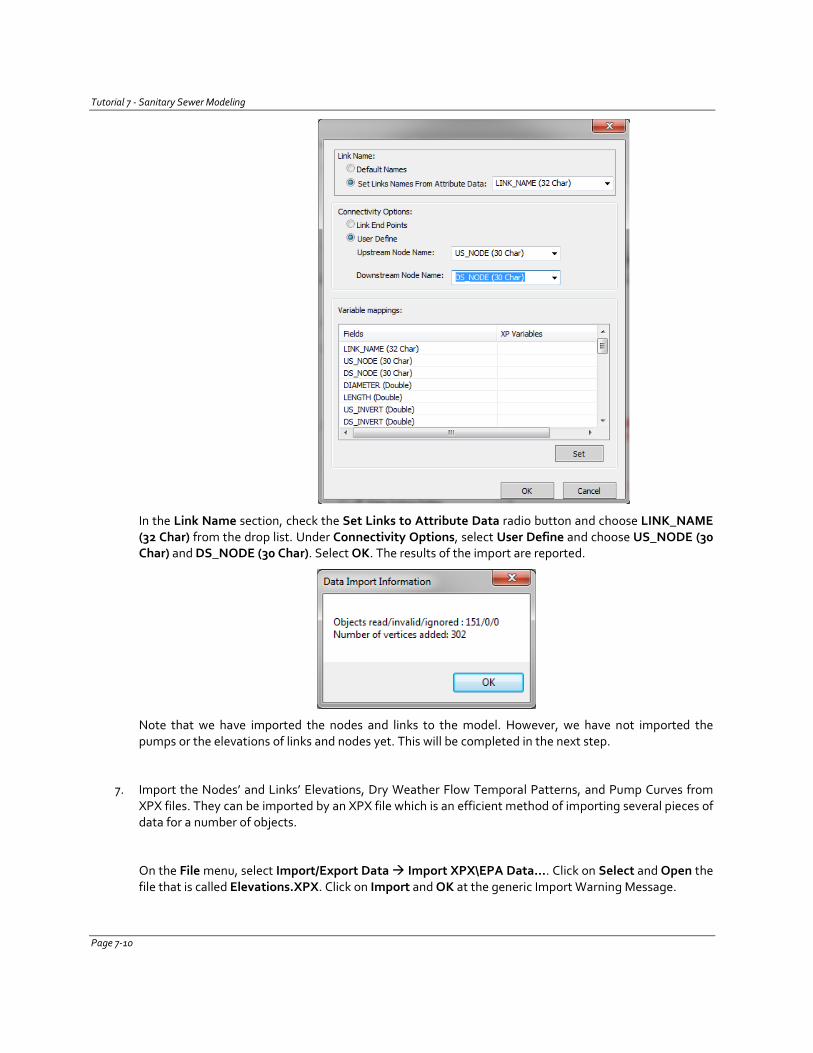
Tutorial 7 - Sanitary Sewer Modeling
In the Link Name section, check the Set Links to Attribute Data radio button and choose LINK_NAME (32 Char) from the drop list. Under Connectivity Options, select User Define and choose US_NODE (30 Char) and DS_NODE (30 Char). Select OK. The results of the import are reported.
Note that we have imported the nodes and links to the model. However, we have not imported the pumps or the elevations of links and nodes yet. This will be completed in the next step.
7. Import the Nodes’ and Links’ Elevations, Dry Weather Flow Temporal Patterns, and Pump Curves from XPX files. They can be imported by an XPX file which is an efficient method of importing several pieces of data for a number of objects.
On the File menu, select Import/Export Data Import XPX\EPA Data…. Click on Select and Open the file that is called Elevations.XPX. Click on Import and OK at the generic Import Warning Message.
Page 7-10
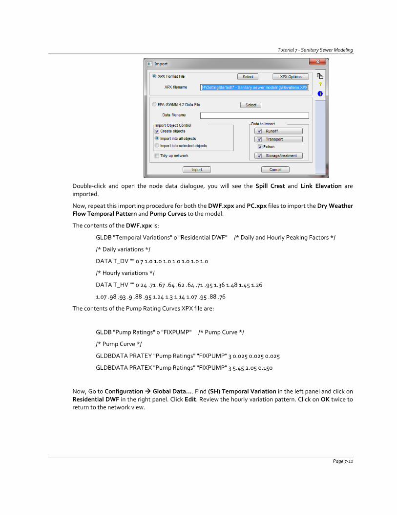
Tutorial 7 - Sanitary Sewer Modeling
Double-click and open the node data dialogue, you will see the Spill Crest and Link Elevation are imported.
Now, repeat this importing procedure for both the DWF.xpx and PC.xpx files to import the Dry Weather Flow Temporal Pattern and Pump Curves to the model.
The contents of the DWF.xpx is:
GLDB "Temporal Variations" 0 "Residential DWF" /* Daily and Hourly Peaking Factors */
/* Daily variations */
DATA T_DV "" 0 7 1.0 1.0 1.0 1.0 1.0 1.0 1.0
/* Hourly variations */
DATA T_HV "" 0 24 .71 .67 .64 .62 .64 .71 .95 1.36 1.48 1.45 1.26
1.07 .98 .93 .9 .88 .95 1.24 1.3 1.14 1.07 .95 .88 .76
The contents of the Pump Rating Curves XPX file are:
GLDB "Pump Ratings" 0 "FIXPUMP" /* Pump Curve */
/* Pump Curve */
GLDBDATA PRATEY "Pump Ratings" "FIXPUMP" 3 0.025 0.025 0.025
GLDBDATA PRATEX "Pump Ratings" "FIXPUMP" 3 5.45 2.05 0.150
Now, Go to Configuration Global Data…. Find (SH) Temporal Variation in the left panel and click on Residential DWF in the right panel. Click Edit. Review the hourly variation pattern. Click on OK twice to return to the network view.
Page 7-11
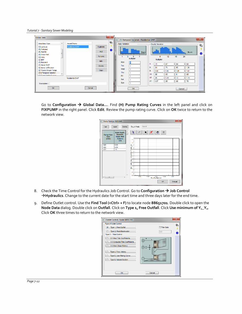
Tutorial 7 - Sanitary Sewer Modeling
Go to Configuration Global Data…. Find (H) Pump Rating Curves in the left panel and click on FIXPUMP in the right panel. Click Edit. Review the pump rating curve. Click on OK twice to return to the network view.
8. Check the Time Control for the Hydraulics Job Control. Go to Configuration Job Control Hydraulics. Change to the current date for the start time and three days later for the end time.
9. Define Outlet control. Use the Find Tool (<Ctrl> + F) to locate node 88651701. Double click to open the Node Data dialog. Double click on Outfall. Click on Type 1, Free Outfall. Click Use minimum of Yc_Yn. Click OK three times to return to the network view.
Page 7-12
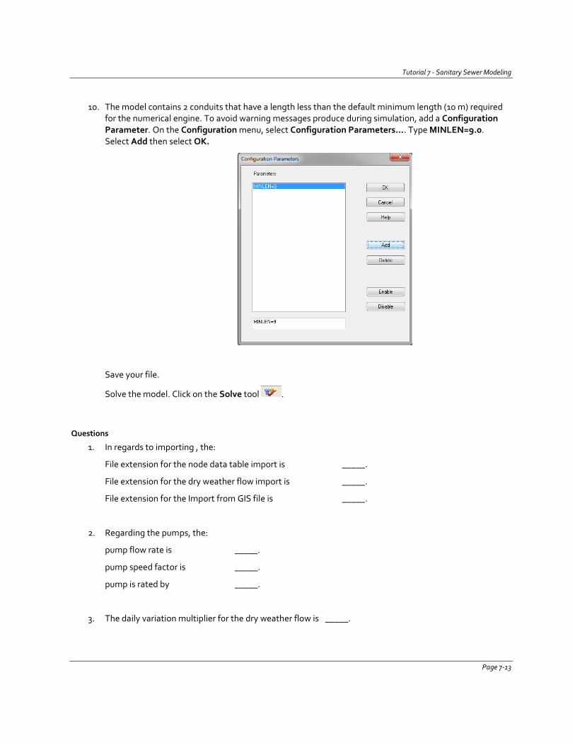
Tutorial 7 - Sanitary Sewer Modeling
10. The model contains 2 conduits that have a length less than the default minimum length (10 m) required for the numerical engine. To avoid warning messages produce during simulation, add a Configuration Parameter. On the Configuration menu, select Configuration Parameters…. Type MINLEN=9.0. Select Add then select OK.
Save your file.
Solve the model. Click on the Solve tool .
Questions
1. In regards to importing , the:
File extension for the node data table import is _____.
File extension for the dry weather flow import is _____.
File extension for the Import from GIS file is _____.
2. Regarding the pumps, the:
pump flow rate is _____.
pump speed factor is _____.
pump is rated by _____.
3. The daily variation multiplier for the dry weather flow is _____.
Page 7-13
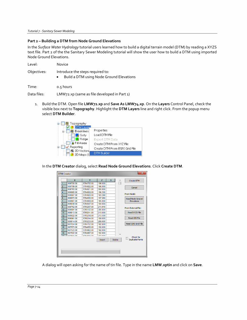
Tutorial 7 - Sanitary Sewer Modeling
Part 2 – Building a DTM from Node Ground Elevations
In the Surface Water Hydrology tutorial users learned how to build a digital terrain model (DTM) by reading a XYZS text file. Part 2 of the the Sanitary Sewer Modeling tutorial will show the user how to build a DTM using imported Node Ground Elevations.
Level: Novice
Objectives: Introduce the steps required to: • Build a DTM using Node Ground Elevations
Time: 0.5 hours
Data files: LMW72.xp (same as file developed in Part 1) 1. Build the DTM. Open file LMW72.xp and Save As LMW74.xp. On the Layers Control Panel, check the
visible box next to Topography. Highlight the DTM Layers line and right click. From the popup menu select DTM Builder.
In the DTM Creator dialog, select Read Node Ground Elevations. Click Create DTM.
A dialog will open asking for the name of tin file. Type in the name LMW.xptin and click on Save.
Page 7-14
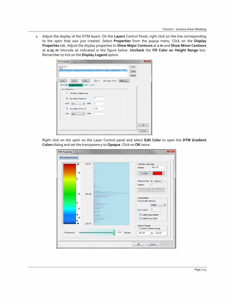
Tutorial 7 - Sanitary Sewer Modeling
2. Adjust the display of the DTM layers. On the Layers Control Panel, right click on the line corresponding to the xptin that was just created. Select Properties from the popup menu. Click on the Display Properties tab. Adjust the display properties to Show Major Contours at 2 m and Show Minor Contours at 0.25 m intervals as indicated in the figure below. Uncheck the Fill Color on Height Range box. Remember to tick on the Display Legend option.
Right click on the xptin on the Layer Control panel and select Edit Color to open the DTM Gradient Colors dialog and set the transparency to Opaque. Click on OK twice.
Page 7-15
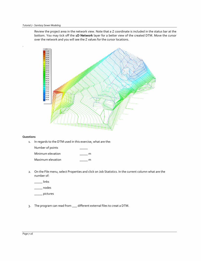
Tutorial 7 - Sanitary Sewer Modeling
Review the project area in the network view. Note that a Z coordinate is included in the status bar at the bottom. You may tick off the 1D Network layer for a better view of the created DTM. Move the cursor over the network and you will see the Z values for the cursor locations.
.
Questions
1. In regards to the DTM used in this exercise, what are the:
Number of points _____
Minimum elevation _____ m
Maximum elevation _____ m
2. On the File menu, select Properties and click on Job Statistics. In the current column what are the number of:
_____ links
_____ nodes
_____ pictures
3. The program can read from ___ different external files to creat a DTM.
Page 7-16
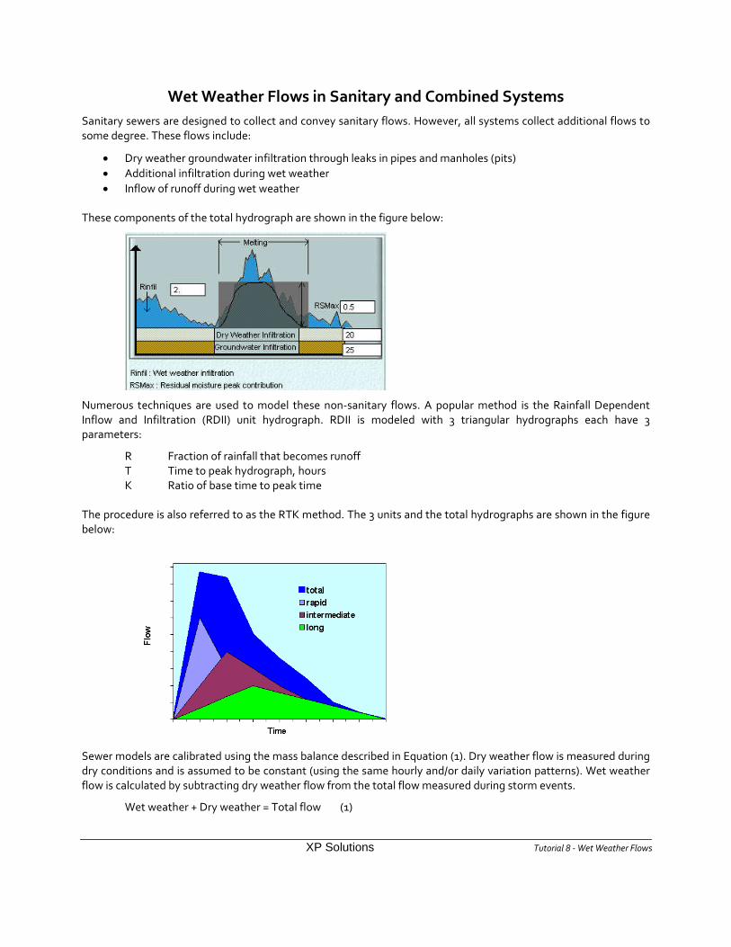
Wet Weather Flows in Sanitary and Combined Systems Sanitary sewers are designed to collect and convey sanitary flows. However, all systems collect additional flows to some degree. These flows include:
• Dry weather groundwater infiltration through leaks in pipes and manholes (pits) • Additional infiltration during wet weather • Inflow of runoff during wet weather
These components of the total hydrograph are shown in the figure below:
Numerous techniques are used to model these non-sanitary flows. A popular method is the Rainfall Dependent Inflow and Infiltration (RDII) unit hydrograph. RDII is modeled with 3 triangular hydrographs each have 3 parameters:
R Fraction of rainfall that becomes runoff T Time to peak hydrograph, hours K Ratio of base time to peak time
The procedure is also referred to as the RTK method. The 3 units and the total hydrographs are shown in the figure below:
Sewer models are calibrated using the mass balance described in Equation (1). Dry weather flow is measured during dry conditions and is assumed to be constant (using the same hourly and/or daily variation patterns). Wet weather flow is calculated by subtracting dry weather flow from the total flow measured during storm events.
Wet weather + Dry weather = Total flow (1)
XP Solutions Tutorial 8 - Wet Weather Flows
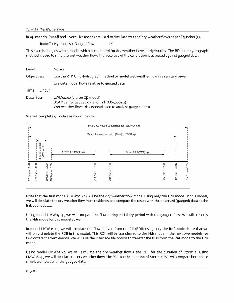
Tutorial 8 - Wet Weather Flows
In xp models, Runoff and Hydraulics modes are used to simulate wet and dry weather flows as per Equation (2).
Runoff + Hydraulics = Gauged flow (2)
This exercise begins with a model which is calibrated for dry weather flows in Hydraulics. The RDII unit hydrograph method is used to simulate wet weather flow. The accuracy of the calibration is assessed against gauged data.
Level: Novice
Objectives: Use the RTK Unit Hydrograph method to model wet weather flow in a sanitary sewer
Evaluate model flows relative to gauged data
Time: 1 hour
Data files: LWM01.xp (starter xp model) 8CAM01.his (gauged data for link 88650601.1) Wet weather flows.xlsx (spread used to analyze gauged data) We will complete 5 models as shown below:
07 S
ept –
11:
40
07 O
ct –
12:
15
07 S
ept –
14:
00
10 S
ept –
12:
00
10 S
ept –
14:
00
21 S
ept –
15:
00
23 S
ept –
18:
00
05 O
ct –
15:
00
Total observation period (Flow) (LMW02.xp)
Initi
al d
ry p
erio
d (L
MW
03.x
p)
Storm 1 (LMW05.xp) Storm 2 (LMW06).xp
09 O
ct –
06:
05
Total observation period (Rainfall) (LMW04.xp)
Note that the first model (LMW02.xp) will be the dry weather flow model using only the Hdr mode. In this model, we will simulate the dry weather flow from residents and compare the result with the observed (gauged) data at the link 88650601.1. Using model LMW03.xp, we will compare the flow during initial dry period with the gauged flow. We will use only the Hdr mode for this model as well. In model LMW04.xp, we will simulate the flow derived from rainfall (RDII) using only the Rnf mode. Note that we will only simulate the RDII in this model. This RDII will be transferred to the Hdr mode in the next two models for two different storm events. We will use the interface file option to transfer the RDII from the Rnf mode to the Hdr mode. Using model LMW05.xp, we will simulate the dry weather flow + the RDII for the duration of Storm 1. Using LMW06.xp, we will simulate the dry weather flow+ the RDII for the duration of Storm 2. We will compare both these simulated flows with the gauged data. Page 8-2
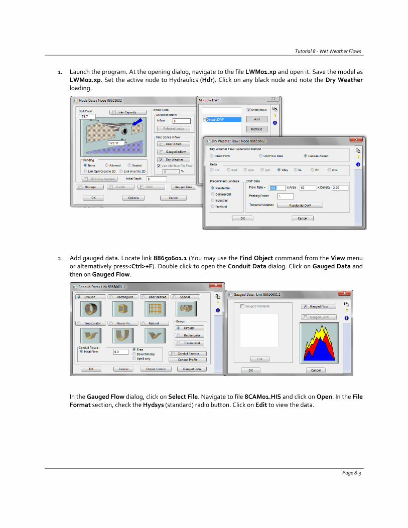
Tutorial 8 - Wet Weather Flows
1. Launch the program. At the opening dialog, navigate to the file LWM01.xp and open it. Save the model as
LWM02.xp. Set the active node to Hydraulics (Hdr). Click on any black node and note the Dry Weather loading.
2. Add gauged data. Locate link 88650601.1 (You may use the Find Object command from the View menu or alternatively press<Ctrl>+F). Double click to open the Conduit Data dialog. Click on Gauged Data and then on Gauged Flow.
In the Gauged Flow dialog, click on Select File. Navigate to file 8CAM01.HIS and click on Open. In the File Format section, check the Hydsys (standard) radio button. Click on Edit to view the data.
Page 8-3
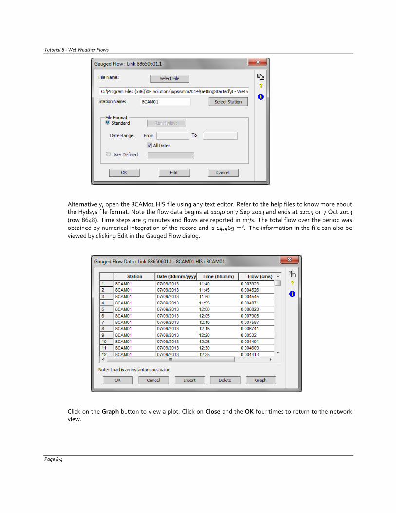
Tutorial 8 - Wet Weather Flows
Alternatively, open the 8CAM01.HIS file using any text editor. Refer to the help files to know more about the Hydsys file format. Note the flow data begins at 11:40 on 7 Sep 2013 and ends at 12:15 on 7 Oct 2013 (row 8648). Time steps are 5 minutes and flows are reported in m3/s. The total flow over the period was obtained by numerical integration of the record and is 14,469 m3. The information in the file can also be viewed by clicking Edit in the Gauged Flow dialog.
Click on the Graph button to view a plot. Click on Close and the OK four times to return to the network view.
Page 8-4
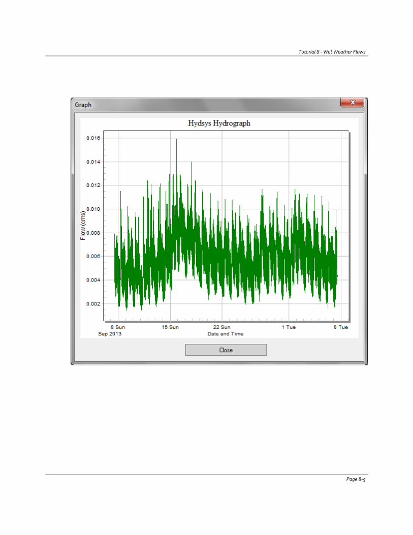
Tutorial 8 - Wet Weather Flows
Page 8-5
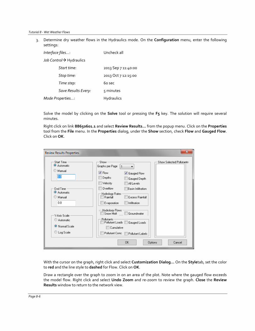
Tutorial 8 - Wet Weather Flows
3. Determine dry weather flows in the Hydraulics mode. On the Configuration menu, enter the following settings:
Interface files…: Uncheck all
Job Control Hydraulics
Start time: 2013 Sep 7 11:40:00
Stop time: 2013 Oct 7 12:15:00
Time step: 60 sec
Save Results Every: 5 minutes
Mode Properties…: Hydraulics
Solve the model by clicking on the Solve tool or pressing the F5 key. The solution will require several minutes.
Right click on link 88650601.1 and select Review Results… from the popup menu. Click on the Properties tool from the File menu. In the Properties dialog, under the Show section, check Flow and Gauged Flow. Click on OK.
With the cursor on the graph, right click and select Customization Dialog… On the Styletab, set the color to red and the line style to dashed for Flow. Click on OK.
Draw a rectangle over the graph to zoom in on an area of the plot. Note where the gauged flow exceeds the model flow. Right click and select Undo Zoom and re-zoom to review the graph. Close the Review Results window to return to the network view.
Page 8-6
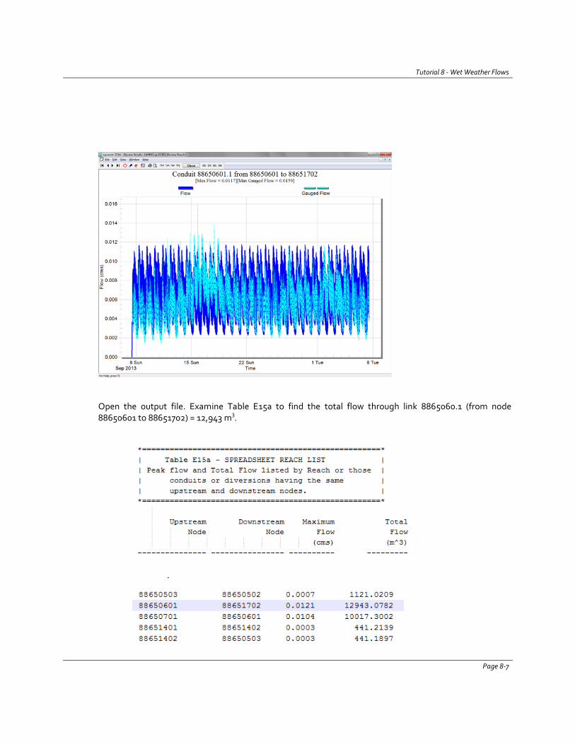
Tutorial 8 - Wet Weather Flows
Open the output file. Examine Table E15a to find the total flow through link 8865060.1 (from node 88650601 to 88651702) = 12,943 m3.
.
Page 8-7
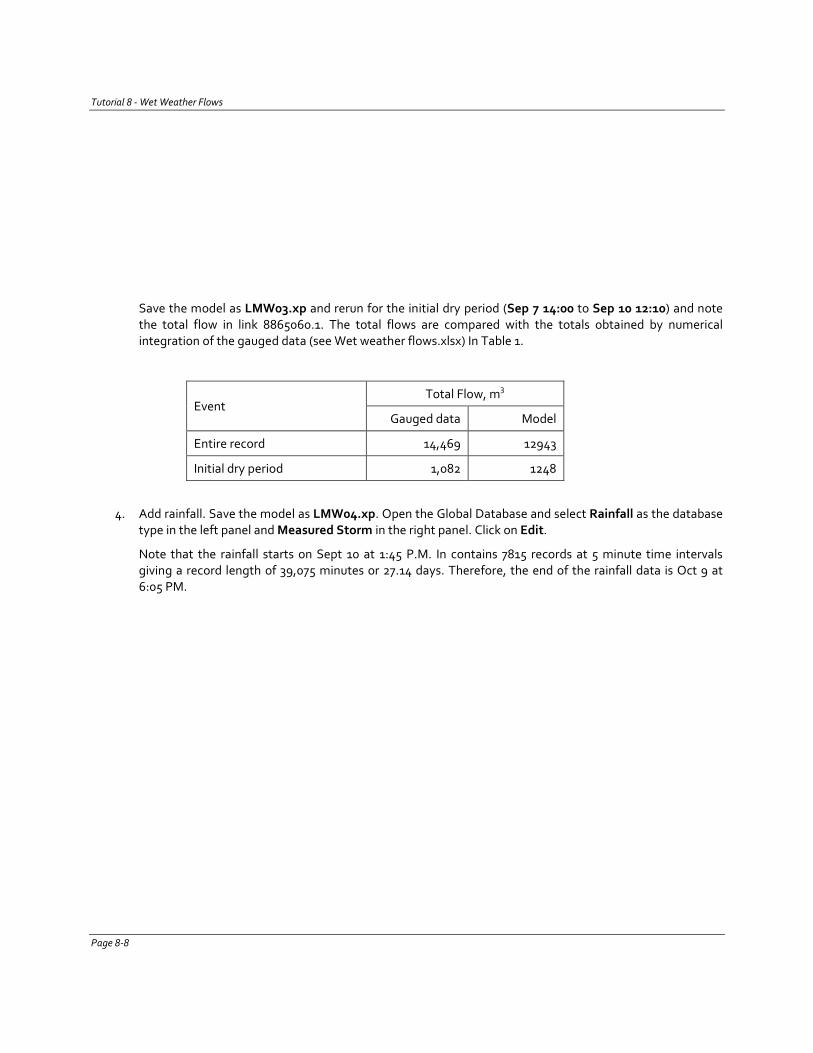
Tutorial 8 - Wet Weather Flows
Save the model as LMW03.xp and rerun for the initial dry period (Sep 7 14:00 to Sep 10 12:10) and note the total flow in link 8865060.1. The total flows are compared with the totals obtained by numerical integration of the gauged data (see Wet weather flows.xlsx) In Table 1.
Event Total Flow, m3
Gauged data Model
Entire record 14,469 12943
Initial dry period 1,082 1248
4. Add rainfall. Save the model as LMW04.xp. Open the Global Database and select Rainfall as the database type in the left panel and Measured Storm in the right panel. Click on Edit.
Note that the rainfall starts on Sept 10 at 1:45 P.M. In contains 7815 records at 5 minute time intervals giving a record length of 39,075 minutes or 27.14 days. Therefore, the end of the rainfall data is Oct 9 at 6:05 PM.
Page 8-8
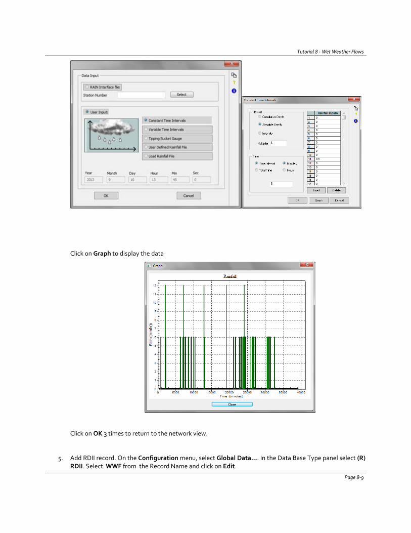
Tutorial 8 - Wet Weather Flows
Click on Graph to display the data
Click on OK 3 times to return to the network view.
5. Add RDII record. On the Configuration menu, select Global Data…. In the Data Base Type panel select (R) RDII. Select WWF from the Record Name and click on Edit.
Page 8-9
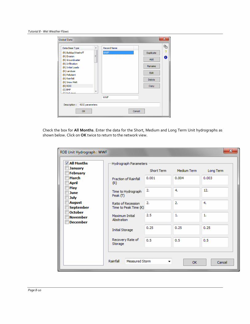
Tutorial 8 - Wet Weather Flows
Check the box for All Months. Enter the data for the Short, Medium and Long Term Unit hydrographs as shown below. Click on OK twice to return to the network view.
Page 8-10
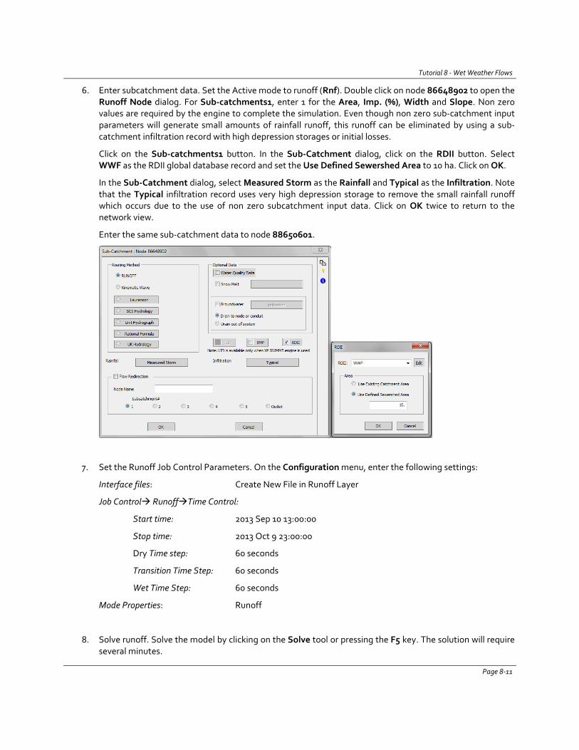
Tutorial 8 - Wet Weather Flows
6. Enter subcatchment data. Set the Active mode to runoff (Rnf). Double click on node 86648902 to open the Runoff Node dialog. For Sub-catchments1, enter 1 for the Area, Imp. (%), Width and Slope. Non zero values are required by the engine to complete the simulation. Even though non zero sub-catchment input parameters will generate small amounts of rainfall runoff, this runoff can be eliminated by using a sub-catchment infiltration record with high depression storages or initial losses.
Click on the Sub-catchments1 button. In the Sub-Catchment dialog, click on the RDII button. Select WWF as the RDII global database record and set the Use Defined Sewershed Area to 10 ha. Click on OK.
In the Sub-Catchment dialog, select Measured Storm as the Rainfall and Typical as the Infiltration. Note that the Typical infiltration record uses very high depression storage to remove the small rainfall runoff which occurs due to the use of non zero subcatchment input data. Click on OK twice to return to the network view.
Enter the same sub-catchment data to node 88650601.
7. Set the Runoff Job Control Parameters. On the Configuration menu, enter the following settings:
Interface files: Create New File in Runoff Layer
Job Control RunoffTime Control:
Start time: 2013 Sep 10 13:00:00
Stop time: 2013 Oct 9 23:00:00
Dry Time step: 60 seconds
Transition Time Step: 60 seconds
Wet Time Step: 60 seconds
Mode Properties: Runoff
8. Solve runoff. Solve the model by clicking on the Solve tool or pressing the F5 key. The solution will require several minutes.
Page 8-11
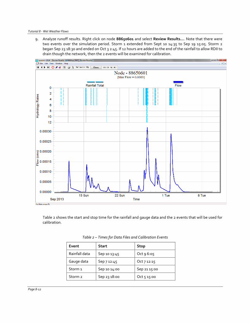
Tutorial 8 - Wet Weather Flows
9. Analyze runoff results. Right click on node 88650601 and select Review Results.... Note that there were two events over the simulation period. Storm 1 extended from Sept 10 14:35 to Sep 19 15:05. Storm 2 began Sep 23 18:30 and ended on Oct 3 2:45. If 12 hours are added to the end of the rainfall to allow RDII to drain though the network, then the 2 events will be examined for calibration.
Table 2 shows the start and stop time for the rainfall and gauge data and the 2 events that will be used for calibration.
Table 2 – Times for Data Files and Calibration Events
Event Start Stop
Rainfall data Sep 10 13:45 Oct 9 6:05
Gauge data Sep 7 12:45 Oct 7 12:15
Storm 1 Sep 10 14:00 Sep 21 15:00
Storm 2 Sep 23 18:00 Oct 5 15:00
Page 8-12
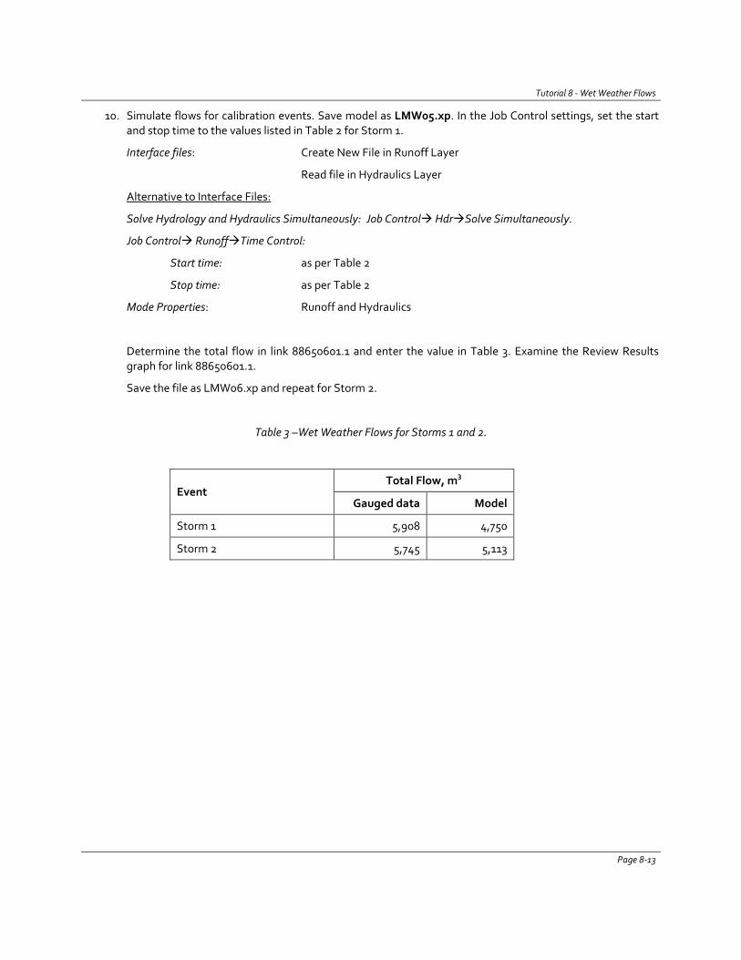
Tutorial 8 - Wet Weather Flows
10. Simulate flows for calibration events. Save model as LMW05.xp. In the Job Control settings, set the start and stop time to the values listed in Table 2 for Storm 1.
Interface files: Create New File in Runoff Layer
Read file in Hydraulics Layer
Alternative to Interface Files:
Solve Hydrology and Hydraulics Simultaneously: Job Control HdrSolve Simultaneously.
Job Control RunoffTime Control:
Start time: as per Table 2
Stop time: as per Table 2
Mode Properties: Runoff and Hydraulics
Determine the total flow in link 88650601.1 and enter the value in Table 3. Examine the Review Results graph for link 88650601.1.
Save the file as LMW06.xp and repeat for Storm 2.
Table 3 –Wet Weather Flows for Storms 1 and 2.
Event Total Flow, m3
Gauged data Model
Storm 1 5,908 4,750
Storm 2 5,745 5,113
Page 8-13

Tutorial 8 - Wet Weather Flows
Questions
1. Comment on the accuracy of the model in regards to sanitary flows. How could the calibration be improved?
2. Comment on the accuracy of the model in regards to wet weather flows. How could the calibration be improved?
Page 8-14
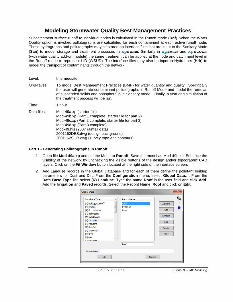
Modeling Stormwater Quality Best Management Practices Subcatchment surface runoff to individual nodes is calculated in the Runoff mode (Rnf). When the Water Quality option is invoked pollutographs are calculated for each contaminant at each active runoff node. These hydrographs and pollutographs may be stored on interface files that are input to the Sanitary Mode (San) to model storage and treatment processes in xpswmm. Similarly in xpswmm and xpstorm (with water quality add-on module) the same treatment can be applied at the node and catchment level in the Runoff mode to represent LID (WSUD). The interface files may also be input to Hydraulics (Hdr) to model the transport of contaminants through the network.
Level: Intermediate
Objectives: To model Best Management Practices (BMP) for water quantity and quality. Specifically the user will generate contaminant pollutographs in Runoff Mode and model the removal of suspended solids and phosphorous in Sanitary mode. Finally, a yearlong simulation of the treatment process will be run.
Time: 1 hour
Data files: Mod-49a.xp (starter file) Mod-49b.xp (Part 1 complete, starter file for part 2) Mod-49c.xp (Part 2 complete, starter file for part 3) Mod-49d.xp (Part 3 complete) Mod-49.his (2007 rainfall data) 2001162DES.dwg (design background) 2001162SUR.dwg (survey topo and contours)
Part 1 - Generating Pollutographs in Runoff
1. Open file Mod-49a.xp and set the Mode to Runoff. Save the model as Mod-49b.xp. Enhance the visibility of the network by unchecking the visible buttons of the design and/or topographic CAD layers. Click on the Fit Window button located at the right side of the interface screen.
2. Add Landuse records in the Global Database and for each of them define the pollutant buildup parameters for Dust and Dirt. From the Configuration menu, select Global Data…. From the Data Base Type list, select (R) Landuse. Type the name Roof in the user field and click Add. Add the Irrigation and Paved records. Select the Record Name: Roof and click on Edit.
XP Solutions Tutorial 9 - BMP Modeling
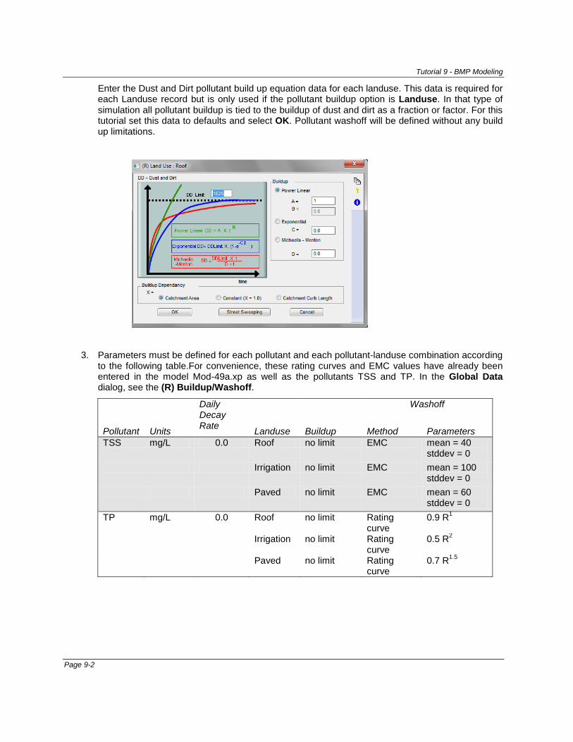
Tutorial 9 - BMP Modeling
Enter the Dust and Dirt pollutant build up equation data for each landuse. This data is required for each Landuse record but is only used if the pollutant buildup option is Landuse. In that type of simulation all pollutant buildup is tied to the buildup of dust and dirt as a fraction or factor. For this tutorial set this data to defaults and select OK. Pollutant washoff will be defined without any build up limitations.
3. Parameters must be defined for each pollutant and each pollutant-landuse combination according to the following table.For convenience, these rating curves and EMC values have already been entered in the model Mod-49a.xp as well as the pollutants TSS and TP. In the Global Data dialog, see the (R) Buildup/Washoff.
Daily Decay Rate
Washoff
Pollutant Units Landuse Buildup Method Parameters TSS mg/L 0.0 Roof no limit EMC mean = 40
stddev = 0 Irrigation no limit EMC mean = 100
stddev = 0 Paved no limit EMC mean = 60
stddev = 0 TP mg/L 0.0 Roof no limit Rating
curve 0.9 R1
Irrigation no limit Rating curve
0.5 R2
Paved no limit Rating curve
0.7 R1.5
Page 9-2
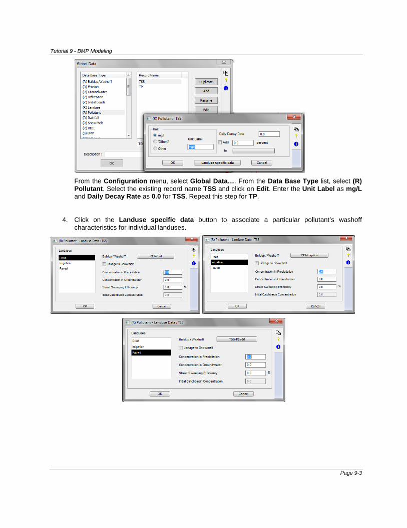
Tutorial 9 - BMP Modeling
From the Configuration menu, select Global Data…. From the Data Base Type list, select (R) Pollutant. Select the existing record name TSS and click on Edit. Enter the Unit Label as mg/L and Daily Decay Rate as 0.0 for TSS. Repeat this step for TP.
4. Click on the Landuse specific data button to associate a particular pollutant’s washoff characteristics for individual landuses.
Page 9-3
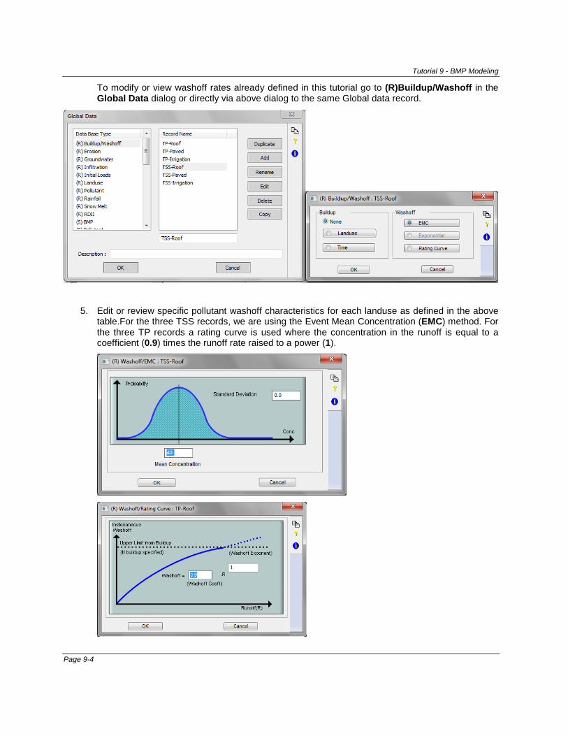
Tutorial 9 - BMP Modeling
To modify or view washoff rates already defined in this tutorial go to (R)Buildup/Washoff in the Global Data dialog or directly via above dialog to the same Global data record.
5. Edit or review specific pollutant washoff characteristics for each landuse as defined in the above table.For the three TSS records, we are using the Event Mean Concentration (EMC) method. For the three TP records a rating curve is used where the concentration in the runoff is equal to a coefficient (0.9) times the runoff rate raised to a power (1).
Page 9-4
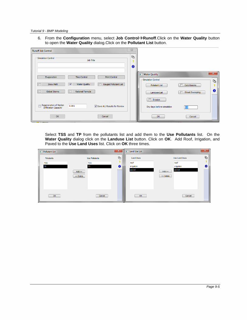
Tutorial 9 - BMP Modeling
6. From the Configuration menu, select Job ControlRunoff.Click on the Water Quality button to open the Water Quality dialog.Click on the Pollutant List button.
Select TSS and TP from the pollutants list and add them to the Use Pollutants list. On the Water Quality dialog click on the Landuse List button. Click on OK. Add Roof, Irrigation, and Paved to the Use Land Uses list. Click on OK three times.
Page 9-5
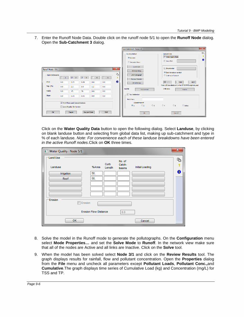
Tutorial 9 - BMP Modeling
7. Enter the Runoff Node Data. Double click on the runoff node 5/1 to open the Runoff Node dialog. Open the Sub-Catchment 3 dialog.
Click on the Water Quality Data button to open the following dialog. Select Landuse, by clicking on blank landuse button and selecting from global data list, making up sub-catchment and type in % of each landuse. Note: For convenience each of these landuse breakdowns have been entered in the active Runoff nodes.Click on OK three times.
8. Solve the model in the Runoff mode to generate the pollutographs. On the Configuration menu select Mode Properties… and set the Solve Mode to Runoff. In the network view make sure that all of the nodes are Active and all links are Inactive. Click on the Solve tool.
9. When the model has been solved select Node 3/1 and click on the Review Results tool. The graph displays results for rainfall, flow and pollutant concentration. Open the Properties dialog from the File menu and uncheck all parameters except Pollutant Loads, Pollutant Conc.,and Cumulative.The graph displays time series of Cumulative Load (kg) and Concentration (mg/L) for TSS and TP.
Page 9-6
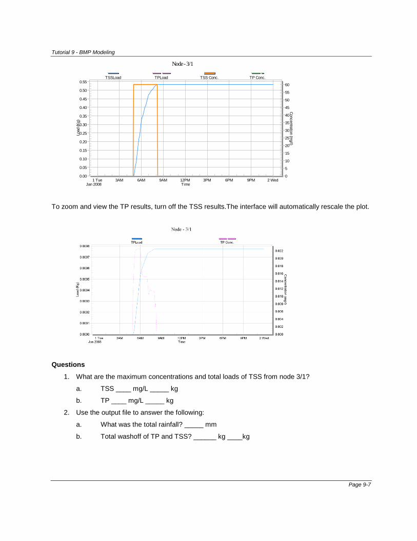
Tutorial 9 - BMP Modeling
To zoom and view the TP results, turn off the TSS results.The interface will automatically rescale the plot.
Questions
1. What are the maximum concentrations and total loads of TSS from node 3/1?
a. TSS ____ mg/L _____ kg
b. TP ____ mg/L _____ kg
2. Use the output file to answer the following:
a. What was the total rainfall? _____ mm
b. Total washoff of TP and TSS? ______ kg ____kg
0.00
0.05
0.10
0.15
0.20
0.25
0.30
0.35
0.40
0.45
0.50
0.55
0
5
10
15
20
25
30
35
40
45
50
55
60
1 TueJan 2008
3AM 6AM 9AM 12PM 3PM 6PM 9PM 2 Wed
Node - 3/1
Load
(Kg)
Concentration (mg/l)
Time
TSSLoad TPLoad TSS Conc. TP Conc.
Page 9-7
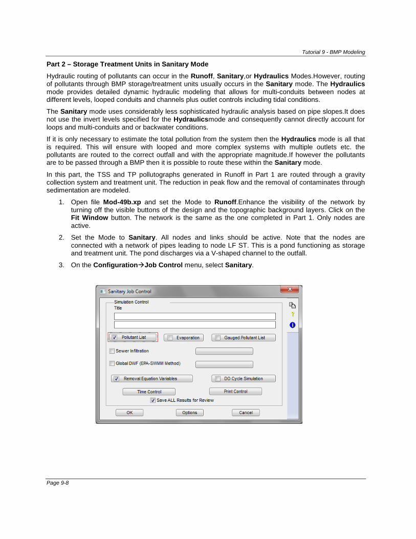
Tutorial 9 - BMP Modeling
Part 2 – Storage Treatment Units in Sanitary Mode
Hydraulic routing of pollutants can occur in the Runoff, Sanitary,or Hydraulics Modes.However, routing of pollutants through BMP storage/treatment units usually occurs in the Sanitary mode. The Hydraulics mode provides detailed dynamic hydraulic modeling that allows for multi-conduits between nodes at different levels, looped conduits and channels plus outlet controls including tidal conditions.
The Sanitary mode uses considerably less sophisticated hydraulic analysis based on pipe slopes.It does not use the invert levels specified for the Hydraulicsmode and consequently cannot directly account for loops and multi-conduits and or backwater conditions.
If it is only necessary to estimate the total pollution from the system then the Hydraulics mode is all that is required. This will ensure with looped and more complex systems with multiple outlets etc. the pollutants are routed to the correct outfall and with the appropriate magnitude.If however the pollutants are to be passed through a BMP then it is possible to route these within the Sanitary mode.
In this part, the TSS and TP pollutographs generated in Runoff in Part 1 are routed through a gravity collection system and treatment unit. The reduction in peak flow and the removal of contaminates through sedimentation are modeled.
1. Open file Mod-49b.xp and set the Mode to Runoff.Enhance the visibility of the network by turning off the visible buttons of the design and the topographic background layers. Click on the Fit Window button. The network is the same as the one completed in Part 1. Only nodes are active.
2. Set the Mode to Sanitary. All nodes and links should be active. Note that the nodes are connected with a network of pipes leading to node LF ST. This is a pond functioning as storage and treatment unit. The pond discharges via a V-shaped channel to the outfall.
3. On the ConfigurationJob Control menu, select Sanitary.
Page 9-8
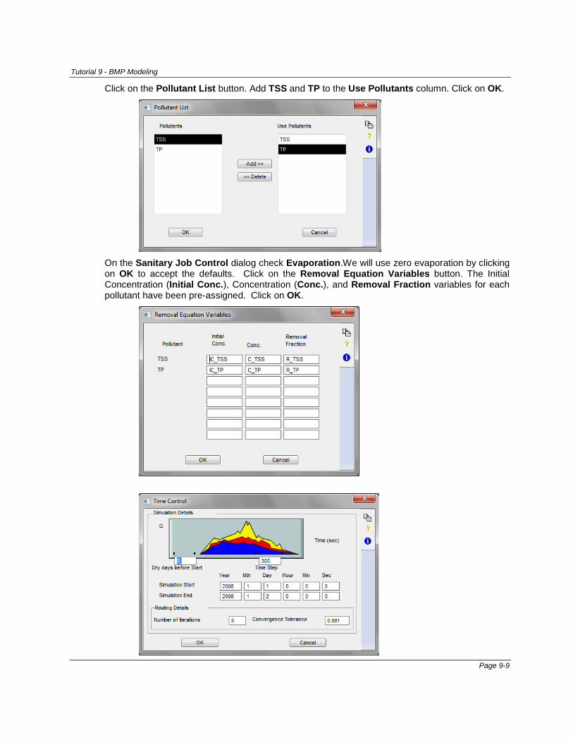
Tutorial 9 - BMP Modeling
Click on the Pollutant List button. Add TSS and TP to the Use Pollutants column. Click on OK.
On the Sanitary Job Control dialog check Evaporation.We will use zero evaporation by clicking on OK to accept the defaults. Click on the Removal Equation Variables button. The Initial Concentration (Initial Conc.), Concentration (Conc.), and Removal Fraction variables for each pollutant have been pre-assigned. Click on OK.
Page 9-9
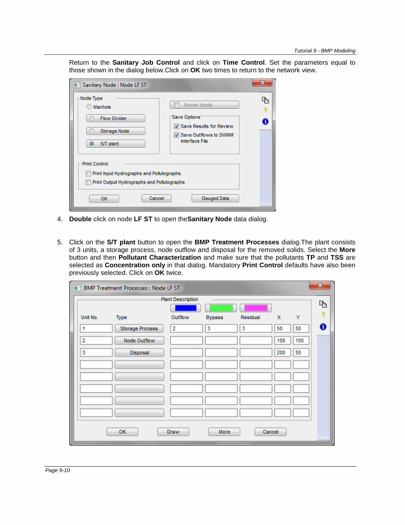
Tutorial 9 - BMP Modeling
Return to the Sanitary Job Control and click on Time Control. Set the parameters equal to those shown in the dialog below.Click on OK two times to return to the network view.
4. Double click on node LF ST to open theSanitary Node data dialog.
5. Click on the S/T plant button to open the BMP Treatment Processes dialog.The plant consists of 3 units, a storage process, node outflow and disposal for the removed solids. Select the More button and then Pollutant Characterization and make sure that the pollutants TP and TSS are selected as Concentration only in that dialog. Mandatory Print Control defaults have also been previously selected. Click on OK twice.
Page 9-10
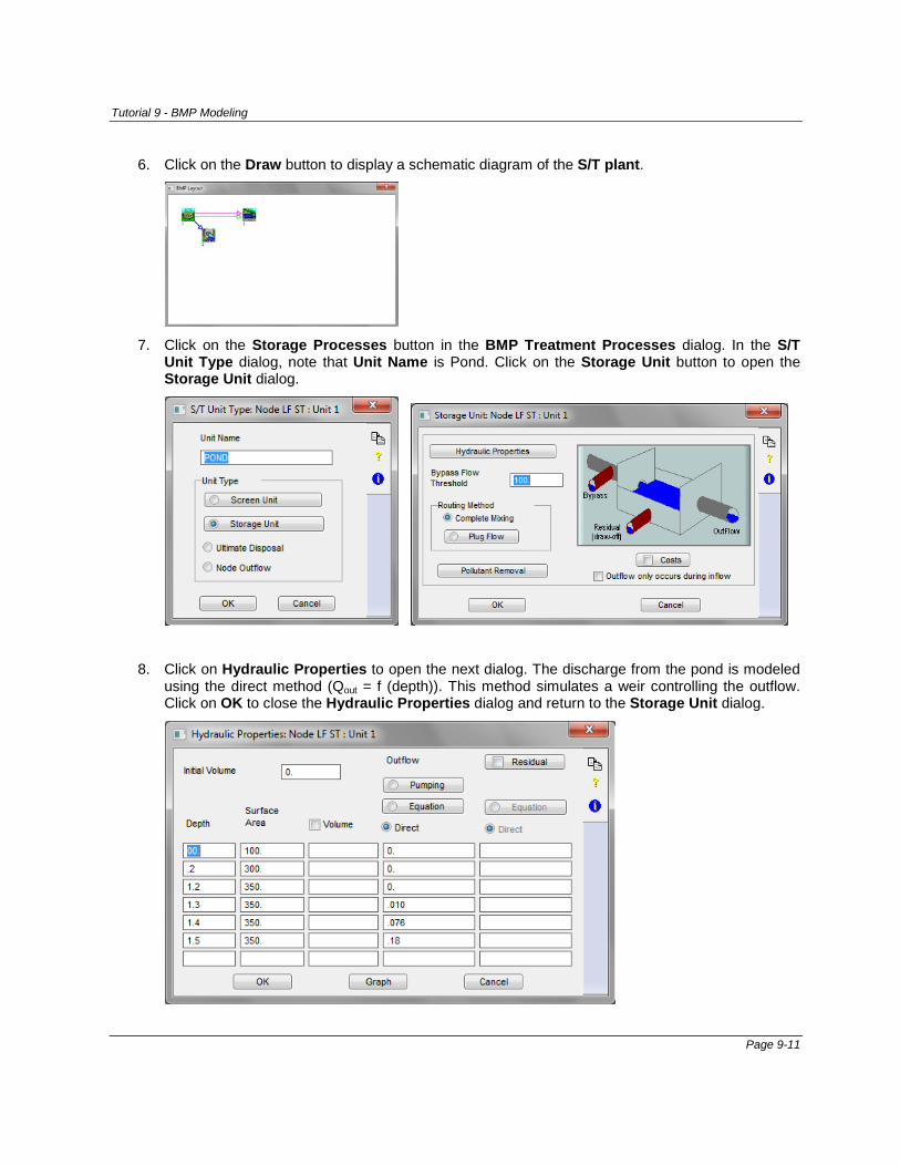
Tutorial 9 - BMP Modeling
6. Click on the Draw button to display a schematic diagram of the S/T plant.
7. Click on the Storage Processes button in the BMP Treatment Processes dialog. In the S/T
Unit Type dialog, note that Unit Name is Pond. Click on the Storage Unit button to open the Storage Unit dialog.
8. Click on Hydraulic Properties to open the next dialog. The discharge from the pond is modeled using the direct method (Qout = f (depth)). This method simulates a weir controlling the outflow. Click on OK to close the Hydraulic Properties dialog and return to the Storage Unit dialog.
Page 9-11
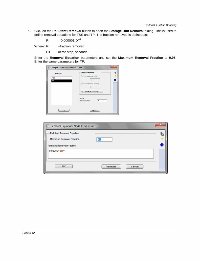
Tutorial 9 - BMP Modeling
9. Click on the Pollutant Removal button to open the Storage Unit Removal dialog. This is used to define removal equations for TSS and TP. The fraction removed is defined as:
R = 0.000001 DT1
Where: R =fraction removed
DT =time step, seconds
Enter the Removal Equation parameters and set the Maximum Removal Fraction to 0.95. Enter the same parameters for TP.
Page 9-12
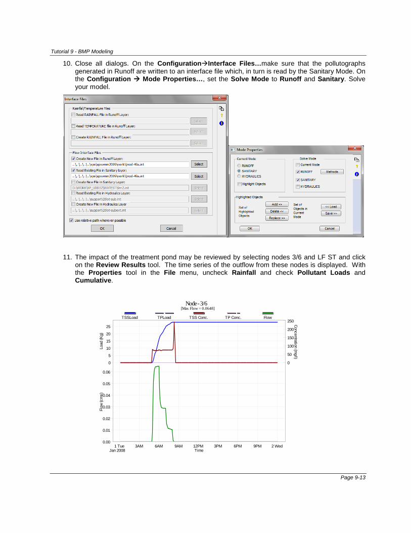
Tutorial 9 - BMP Modeling
10. Close all dialogs. On the ConfigurationInterface Files…make sure that the pollutographs generated in Runoff are written to an interface file which, in turn is read by the Sanitary Mode. On the Configuration Mode Properties…, set the Solve Mode to Runoff and Sanitary. Solve your model.
11. The impact of the treatment pond may be reviewed by selecting nodes 3/6 and LF ST and click on the Review Results tool. The time series of the outflow from these nodes is displayed. With the Properties tool in the File menu, uncheck Rainfall and check Pollutant Loads and Cumulative.
0
5
10
15
20
25
0
50
100
150
200
250
0.00
0.01
0.02
0.03
0.04
0.05
0.06
1 TueJan 2008
3AM 6AM 9AM 12PM 3PM 6PM 9PM 2 Wed
Node - 3/6[Max Flow = 0.0648]
Load
(Kg)
Concentration (mg/l)
Flow
(cm
s)
Time
TSSLoad TPLoad TSS Conc. TP Conc. Flow
Page 9-13
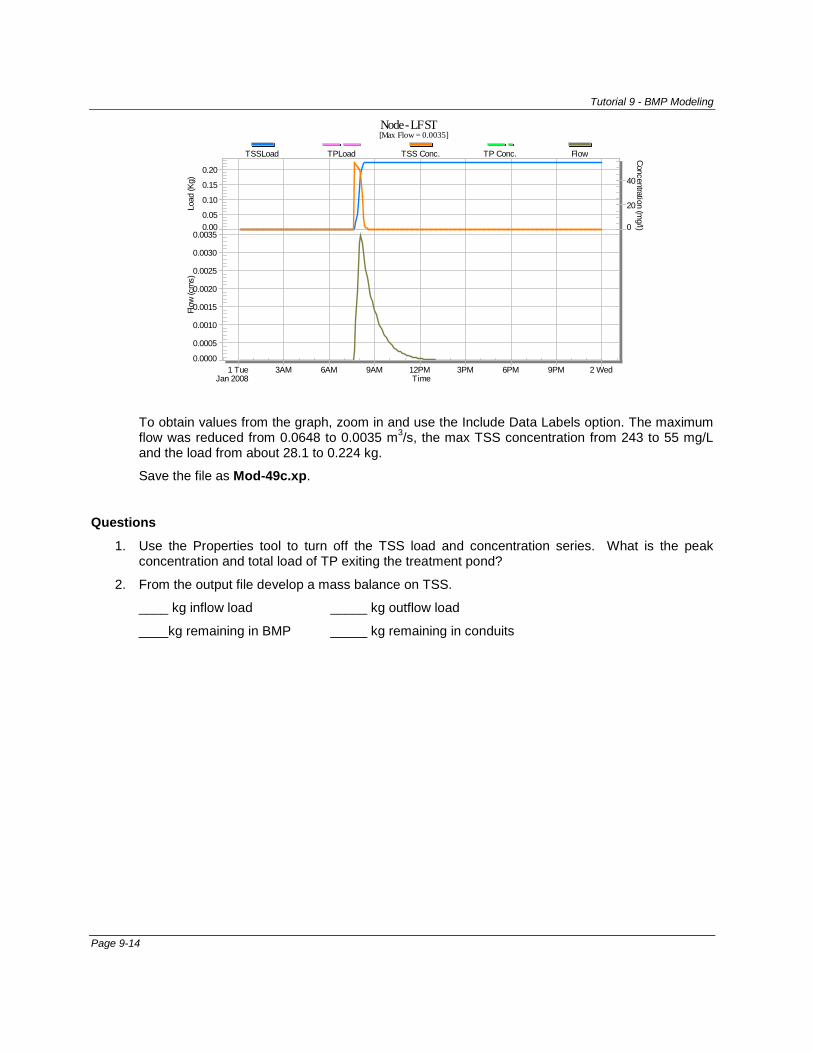
Tutorial 9 - BMP Modeling
To obtain values from the graph, zoom in and use the Include Data Labels option. The maximum flow was reduced from 0.0648 to 0.0035 m3/s, the max TSS concentration from 243 to 55 mg/L and the load from about 28.1 to 0.224 kg.
Save the file as Mod-49c.xp.
Questions
1. Use the Properties tool to turn off the TSS load and concentration series. What is the peak concentration and total load of TP exiting the treatment pond?
2. From the output file develop a mass balance on TSS.
____ kg inflow load _____ kg outflow load
____kg remaining in BMP _____ kg remaining in conduits
0.000.05
0.10
0.15
0.20
0
20
40
0.0000
0.0005
0.0010
0.0015
0.0020
0.0025
0.0030
0.0035
1 TueJan 2008
3AM 6AM 9AM 12PM 3PM 6PM 9PM 2 Wed
Node - LF ST[Max Flow = 0.0035]
Load
(Kg)
Concentration (mg/l)
Flow
(cm
s)
Time
TSSLoad TPLoad TSS Conc. TP Conc. Flow
Page 9-14
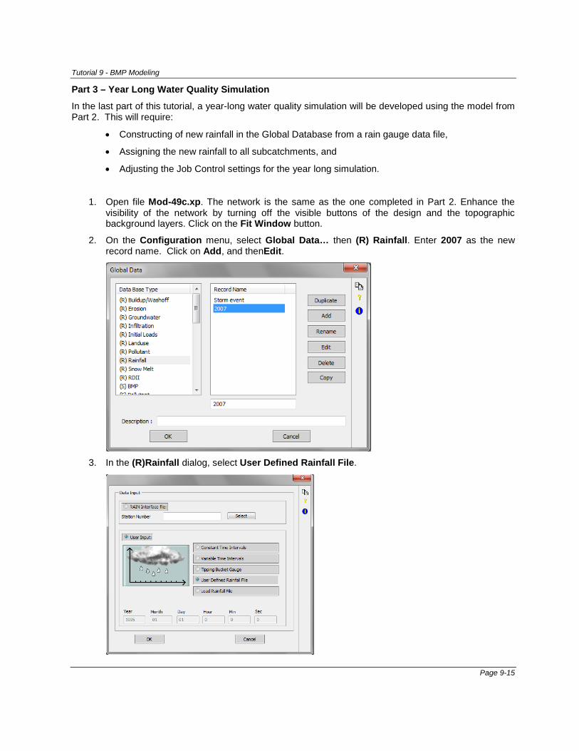
Tutorial 9 - BMP Modeling
Part 3 – Year Long Water Quality Simulation
In the last part of this tutorial, a year-long water quality simulation will be developed using the model from Part 2. This will require:
• Constructing of new rainfall in the Global Database from a rain gauge data file,
• Assigning the new rainfall to all subcatchments, and
• Adjusting the Job Control settings for the year long simulation.
1. Open file Mod-49c.xp. The network is the same as the one completed in Part 2. Enhance the visibility of the network by turning off the visible buttons of the design and the topographic background layers. Click on the Fit Window button.
2. On the Configuration menu, select Global Data… then (R) Rainfall. Enter 2007 as the new record name. Click on Add, and thenEdit.
3. In the (R)Rainfall dialog, select User Defined Rainfall File.
Page 9-15
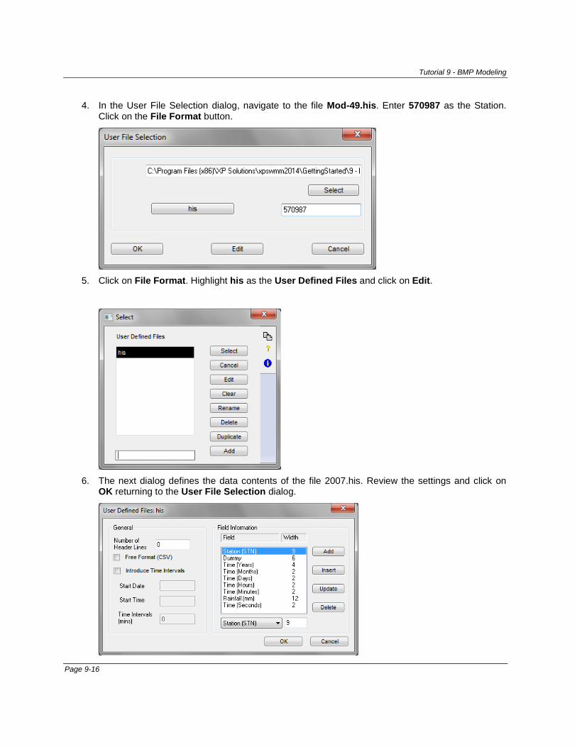
Tutorial 9 - BMP Modeling
4. In the User File Selection dialog, navigate to the file Mod-49.his. Enter 570987 as the Station. Click on the File Format button.
5. Click on File Format. Highlight his as the User Defined Files and click on Edit.
6. The next dialog defines the data contents of the file 2007.his. Review the settings and click on
OK returning to the User File Selection dialog.
Page 9-16
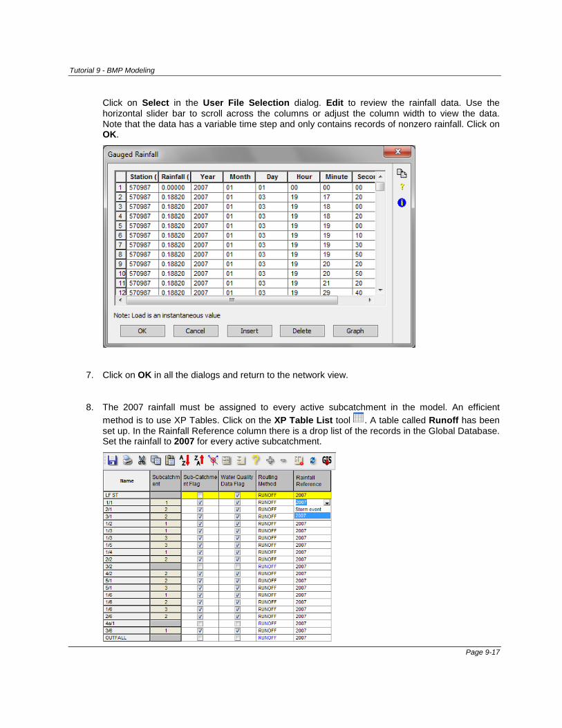
Tutorial 9 - BMP Modeling
Click on Select in the User File Selection dialog. Edit to review the rainfall data. Use the horizontal slider bar to scroll across the columns or adjust the column width to view the data. Note that the data has a variable time step and only contains records of nonzero rainfall. Click on OK.
7. Click on OK in all the dialogs and return to the network view.
8. The 2007 rainfall must be assigned to every active subcatchment in the model. An efficient method is to use XP Tables. Click on the XP Table List tool . A table called Runoff has been set up. In the Rainfall Reference column there is a drop list of the records in the Global Database. Set the rainfall to 2007 for every active subcatchment.
Page 9-17
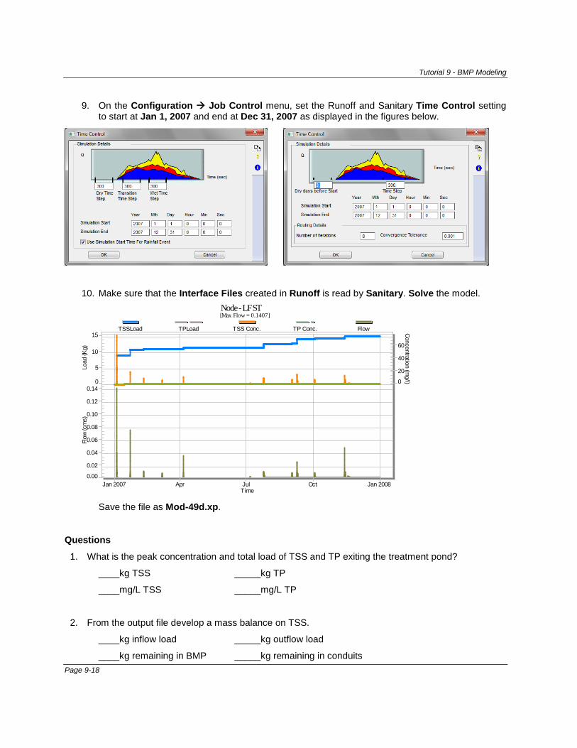
Tutorial 9 - BMP Modeling
9. On the Configuration Job Control menu, set the Runoff and Sanitary Time Control setting to start at Jan 1, 2007 and end at Dec 31, 2007 as displayed in the figures below.
10. Make sure that the Interface Files created in Runoff is read by Sanitary. Solve the model.
Save the file as Mod-49d.xp.
Questions
1. What is the peak concentration and total load of TSS and TP exiting the treatment pond?
____kg TSS _____kg TP
____mg/L TSS _____mg/L TP
2. From the output file develop a mass balance on TSS.
____kg inflow load _____kg outflow load
____kg remaining in BMP _____kg remaining in conduits
0
5
10
15
0
20
40
60
0.00
0.02
0.04
0.06
0.08
0.10
0.12
0.14
Jan 2007 Apr Jul Oct Jan 2008
Node - LF ST[Max Flow = 0.1407]
Load
(Kg)
Concentration (mg/l)
Flow
(cm
s)
Time
TSSLoad TPLoad TSS Conc. TP Conc. Flow
Page 9-18

Creating Design Storms and Using Global Storms
Modelers frequently use design storms to evaluate existing and proposed stormwater management systems. Design storms vary by geographic location and are typically designated by duration and frequency such as the 10-year, 24-hour storm. Modelers are encouraged to consult local regulations and design manuals to obtain the appropriate design storms for their systems.
It is common practice to evaluate the performance of systems against multiple design storms. The Global Storms tool in the xp interface allows users to analyze several storms simultaneously and to compare results on a single graph.
Global data from any xp model can be merged with another model. This example demonstrates adding a design storm using the SCS Type II distribution. This is a unit hyetograph that is used in the United States. A multiplier is applied to the hyetograph to customize the storm at a specific location and return period.
The Global Storms tool is used to quickly add a series of storms to a model. Multiple storm events can then be solved simultaneously and the results can be compared on a single graph.
Level: Novice
Objectives: Merge global data from another model Customize a unit hyetograph Use the Global Storms tool to simultaneously solve multiple storms
Time: 0.5 hour
Data Files: SCS_Storms.xp (starter file) Global Storms – SCS.xp (contains SCS storms)
Part 1 - Adding a Design Storm with File Merge
1. Launch xpswmm. Open file SCS_Storms.
2. On the File menu, select Merge. In the Merge Database dialog, check only Merge Global Database. Click on File.
3. In Windows Explorer, navigate to the Samples folder and select Global Storms - SCS.xp. Click on Open.
4. Create new Global Data record. On the Configuration menu select Global Data. Select (R) Rainfall from the Data Base Type panel. Highlight SCS Type II as the record name and click on
XP Solutions Tutorial 10 - Design and Global Storms
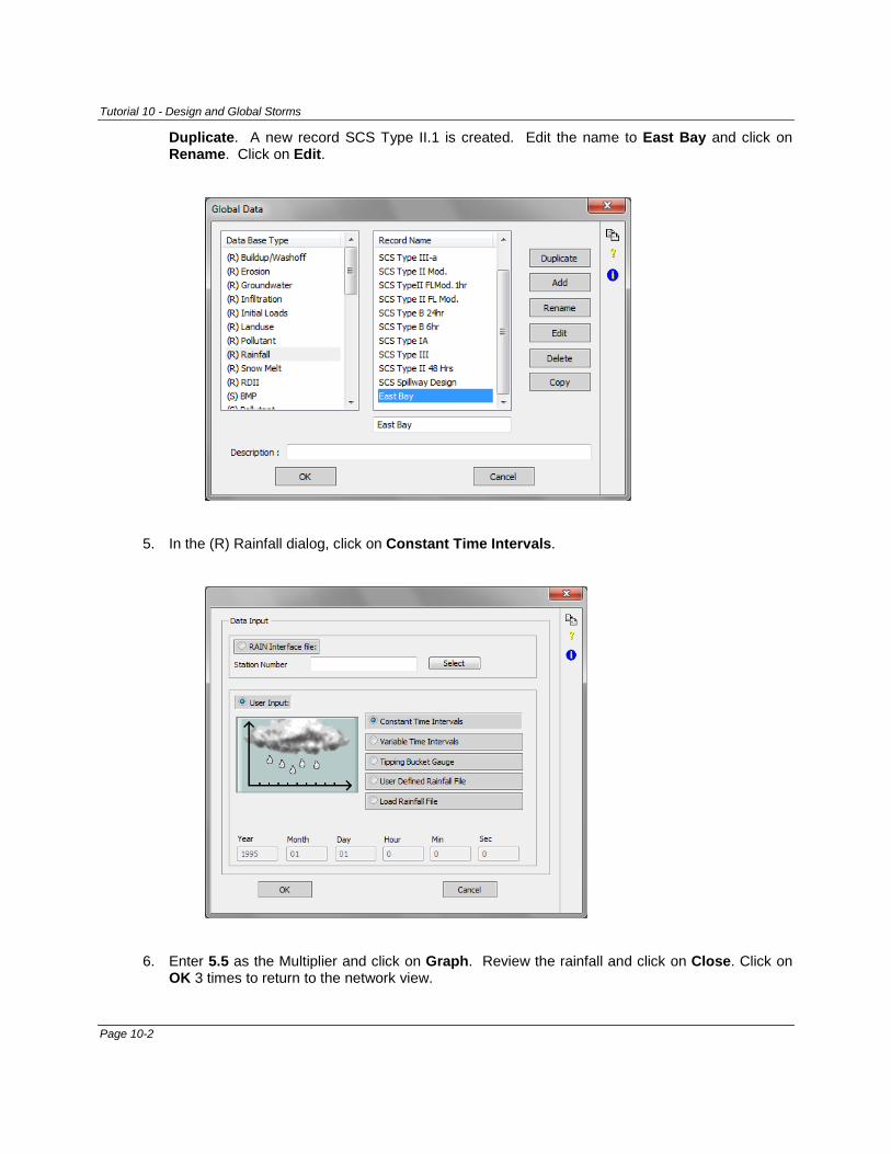
Tutorial 10 - Design and Global Storms
Duplicate. A new record SCS Type II.1 is created. Edit the name to East Bay and click on Rename. Click on Edit.
5. In the (R) Rainfall dialog, click on Constant Time Intervals.
6. Enter 5.5 as the Multiplier and click on Graph. Review the rainfall and click on Close. Click on OK 3 times to return to the network view.
Page 10-2
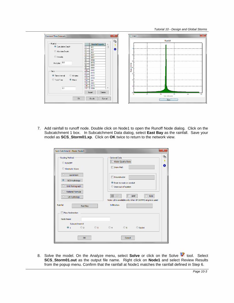
Tutorial 10 - Design and Global Storms
7. Add rainfall to runoff node. Double click on Node1 to open the Runoff Node dialog. Click on the Subcatchment 1 box. In Subcatchment Data dialog, select East Bay as the rainfall. Save your model as SCS_Storm01.xp. Click on OK twice to return to the network view.
8. Solve the model. On the Analyze menu, select Solve or click on the Solve tool. Select SCS_Storm01.out as the output file name. Right click on Node1 and select Review Results from the popup menu. Confirm that the rainfall at Node1 matches the rainfall defined in Step 6.
Page 10-3
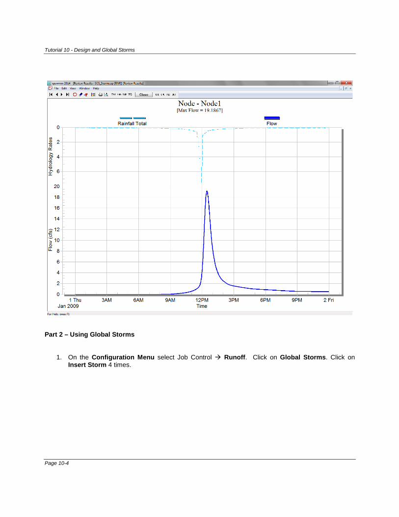
Tutorial 10 - Design and Global Storms
Part 2 – Using Global Storms
1. On the Configuration Menu select Job Control Runoff. Click on Global Storms. Click on Insert Storm 4 times.
Page 10-4
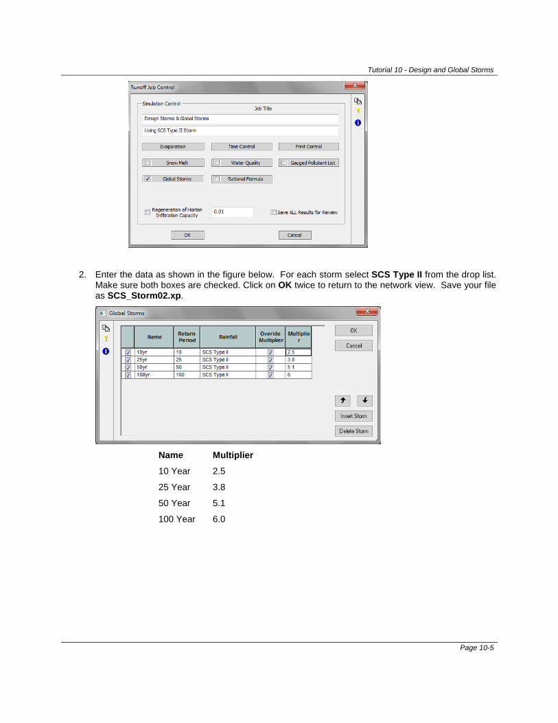
Tutorial 10 - Design and Global Storms
2. Enter the data as shown in the figure below. For each storm select SCS Type II from the drop list. Make sure both boxes are checked. Click on OK twice to return to the network view. Save your file as SCS_Storm02.xp.
Name Multiplier
10 Year 2.5
25 Year 3.8
50 Year 5.1
100 Year 6.0
Page 10-5
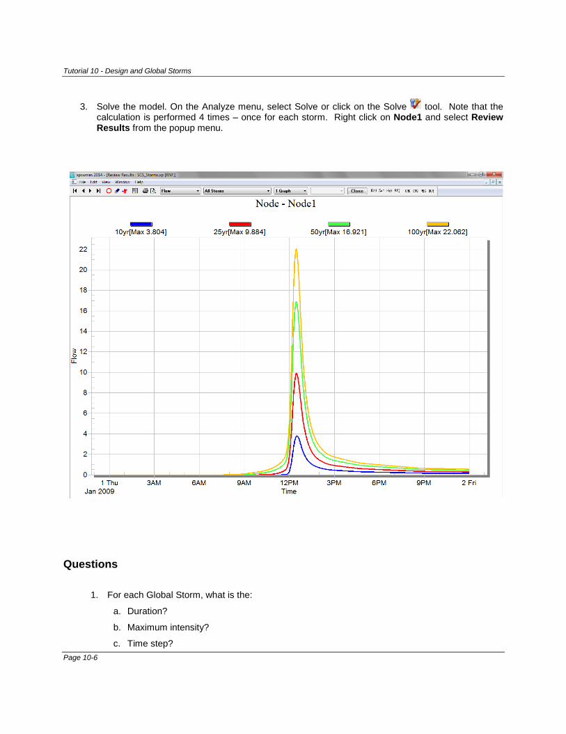
Tutorial 10 - Design and Global Storms
3. Solve the model. On the Analyze menu, select Solve or click on the Solve tool. Note that the calculation is performed 4 times – once for each storm. Right click on Node1 and select Review Results from the popup menu.
Questions
1. For each Global Storm, what is the:
a. Duration?
b. Maximum intensity?
c. Time step? Page 10-6
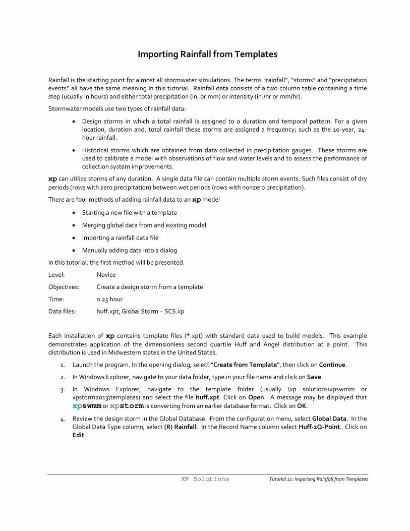
Importing Rainfall from Templates
Rainfall is the starting point for almost all stormwater simulations. The terms “rainfall”, “storms” and “precipitation events” all have the same meaning in this tutorial. Rainfall data consists of a two column table containing a time step (usually in hours) and either total precipitation (in. or mm) or intensity (in./hr or mm/hr).
Stormwater models use two types of rainfall data:
• Design storms in which a total rainfall is assigned to a duration and temporal pattern. For a given location, duration and, total rainfall these storms are assigned a frequency; such as the 10-year, 24-hour rainfall.
• Historical storms which are obtained from data collected in precipitation gauges. These storms are used to calibrate a model with observations of flow and water levels and to assess the performance of collection system improvements.
xp can utilize storms of any duration. A single data file can contain multiple storm events. Such files consist of dry periods (rows with zero precipitation) between wet periods (rows with nonzero precipitation).
There are four methods of adding rainfall data to an xp model
• Starting a new file with a template
• Merging global data from and existing model
• Importing a rainfall data file
• Manually adding data into a dialog
In this tutorial, the first method will be presented.
Level: Novice
Objectives: Create a design storm from a template
Time: 0.25 hour
Data files: huff.xpt, Global Storm – SCS.xp
Each installation of xp contains template files (*.xpt) with standard data used to build models. This example demonstrates application of the dimensionless second quartile Huff and Angel distribution at a point. This distribution is used in Midwestern states in the United States.
1. Launch the program. In the opening dialog, select “Create from Template”, then click on Continue.
2. In Windows Explorer, navigate to your data folder, type in your file name and click on Save.
3. In Windows Explorer, navigate to the template folder (usually \xp solutions\xpswmm or xpstorm2013\templates) and select the file huff.xpt. Click on Open. A message may be displayed that xpswmm or xpstorm is converting from an earlier database format. Click on OK.
4. Review the design storm in the Global Database. From the configuration menu, select Global Data. In the Global Data Type column, select (R) Rainfall. In the Record Name column select Huff-2Q-Point. Click on Edit.
XP Solutions Tutorial 11: Importing Rainfall from Templates
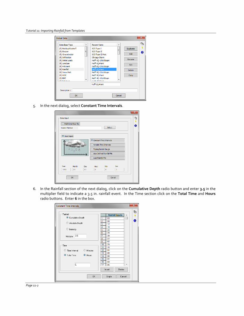
Tutorial 11: Importing Rainfall from Templates
5. In the next dialog, select Constant Time Intervals.
6. In the Rainfall section of the next dialog, click on the Cumulative Depth radio button and enter 3.5 in the multiplier field to indicate a 3.5 in. rainfall event. In the Time section click on the Total Time and Hours radio buttons. Enter 6 in the box.
Page 11-2
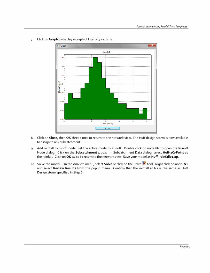
Tutorial 11: Importing Rainfall from Templates
7. Click on Graph to display a graph of Intensity vs. time.
8. Click on Close, then OK three times to return to the network view. The Huff design storm is now available to assign to any subcatchment.
9. Add rainfall to runoff node. Set the active mode to Runoff. Double click on node N1 to open the Runoff Node dialog. Click on the Subcatchment 1 box. In Subcatchment Data dialog, select Huff-2Q-Point as the rainfall. Click on OK twice to return to the network view. Save your model as Huff_rainfall01.xp.
10. Solve the model. On the Analyze menu, select Solve or click on the Solve tool. Right click on node N1 and select Review Results from the popup menu. Confirm that the rainfall at N1 is the same as Huff Design storm specified in Step 6.
Page11-3
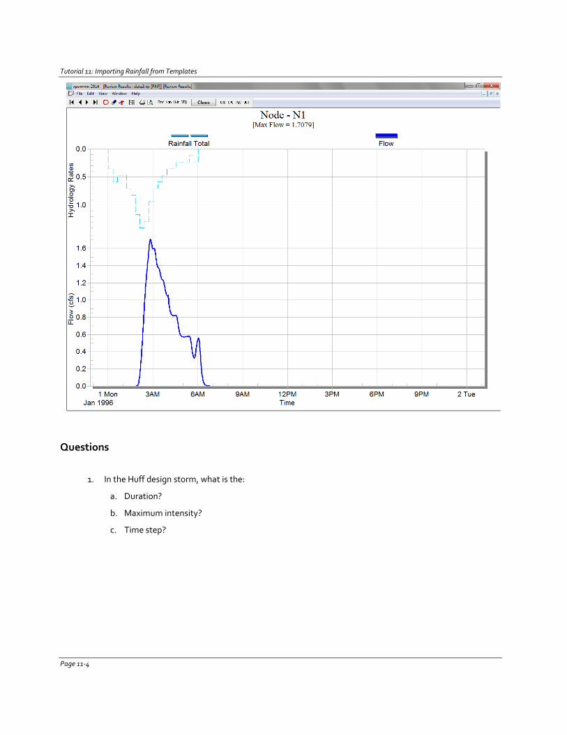
Tutorial 11: Importing Rainfall from Templates
Questions
1. In the Huff design storm, what is the:
a. Duration?
b. Maximum intensity?
c. Time step?
Page 11-4
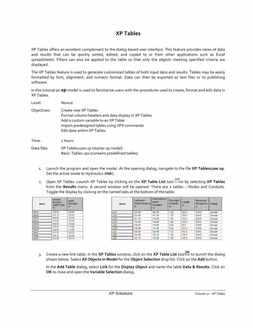
XP Tables
XP Tables offers an excellent complement to the dialog-based user interface. This feature provides views of data and results that can be quickly sorted, edited, and copied to or from other applications such as Excel spreadsheets. Filters can also be applied to the table so that only the objects meeting specified criteria are displayed.
The XP Tables feature is used to generate customized tables of both input data and results. Tables may be easily formatted by font, alignment, and numeric format. Data can then be exported as text files or to publishing software.
In this tutorial an xp model is used to familiarize users with the procedures used to create, format and edit data in XP Tables.
Level: Novice
Objectives: Create new XP Tables Format column headers and data display in XP Tables Add a custom variable to an XP Table Import predesigned tables using XPX commands Edit data within XP Tables Time: 2 hours
Data files: XP Tables1200.xp (starter xp model) Basic-Tables.xpx (contains predefined tables)
1. Launch the program and open the model. At the opening dialog, navigate to the file XP Tables1200.xp. Set the active mode to Hydraulics (Hdr).
2. Open XP Tables. Launch XP Tables by clicking on the XP Table List tool or by selecting XP Tables from the Results menu. A second window will be opened. There are 2 tables – Nodes and Conduits. Toggle the display by clicking on the named tabs at the bottom of the table.
3. Create a new link table. In the XP Tables window, click on the XP Table List tool to launch the dialog shown below. Select All Objects in Model for the Object Selection drop list. Click on the Add button.
In the Add Table dialog, select Link for the Display Object and name the table Data & Results. Click on OK to close and open the Variable Selection dialog.
XP Solutions Tutorial 12 – XP Tables
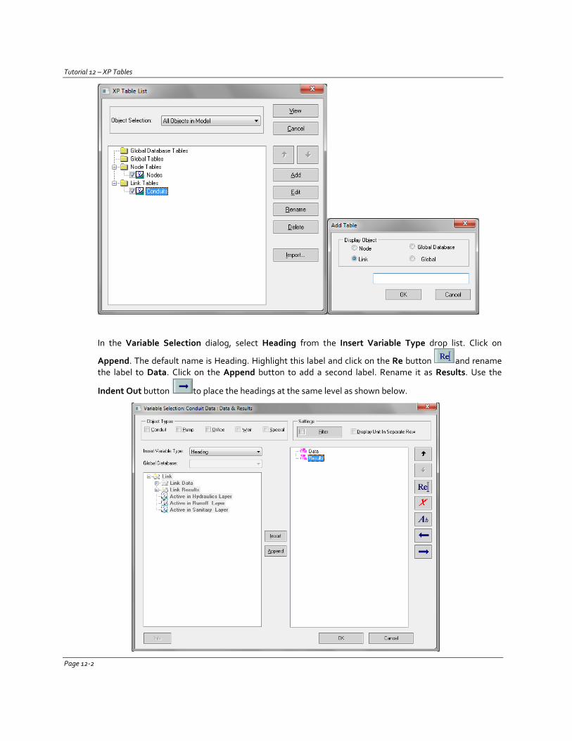
Tutorial 12 – XP Tables
In the Variable Selection dialog, select Heading from the Insert Variable Type drop list. Click on
Append. The default name is Heading. Highlight this label and click on the Re button and rename the label to Data. Click on the Append button to add a second label. Rename it as Results. Use the
Indent Out button to place the headings at the same level as shown below.
Page 12-2
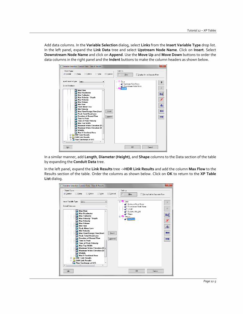
Tutorial 12 – XP Tables
Add data columns. In the Variable Selection dialog, select Links from the Insert Variable Type drop list. In the left panel, expand the Link Data tree and select Upstream Node Name. Click on Insert. Select Downstream Node Name and click on Append. Use the Move Up and Move Down buttons to order the data columns in the right panel and the Indent buttons to make the column headers as shown below.
In a similar manner, add Length, Diameter (Height), and Shape columns to the Data section of the table by expanding the Conduit Data tree.
In the left panel, expand the Link Results tree ->HDR Link Results and add the column Max Flow to the Results section of the table. Order the columns as shown below. Click on OK to return to the XP Table List dialog.
Page 12-3
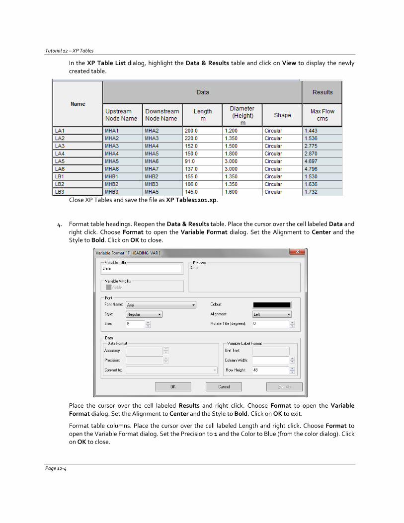
Tutorial 12 – XP Tables
In the XP Table List dialog, highlight the Data & Results table and click on View to display the newly created table.
Close XP Tables and save the file as XP Tables1201.xp.
4. Format table headings. Reopen the Data & Results table. Place the cursor over the cell labeled Data and right click. Choose Format to open the Variable Format dialog. Set the Alignment to Center and the Style to Bold. Click on OK to close.
Place the cursor over the cell labeled Results and right click. Choose Format to open the Variable Format dialog. Set the Alignment to Center and the Style to Bold. Click on OK to exit.
Format table columns. Place the cursor over the cell labeled Length and right click. Choose Format to open the Variable Format dialog. Set the Precision to 1 and the Color to Blue (from the color dialog). Click on OK to close.
Page 12-4
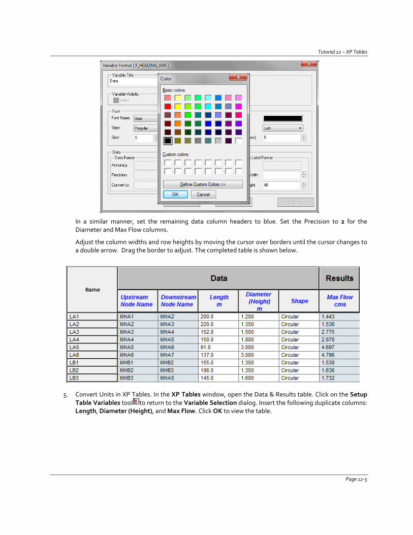
Tutorial 12 – XP Tables
In a similar manner, set the remaining data column headers to blue. Set the Precision to 2 for the Diameter and Max Flow columns.
Adjust the column widths and row heights by moving the cursor over borders until the cursor changes to a double arrow. Drag the border to adjust. The completed table is shown below.
5. Convert Units in XP Tables. In the XP Tables window, open the Data & Results table. Click on the Setup Table Variables tool to return to the Variable Selection dialog. Insert the following duplicate columns: Length, Diameter (Height), and Max Flow. Click OK to view the table.
Page 12-5
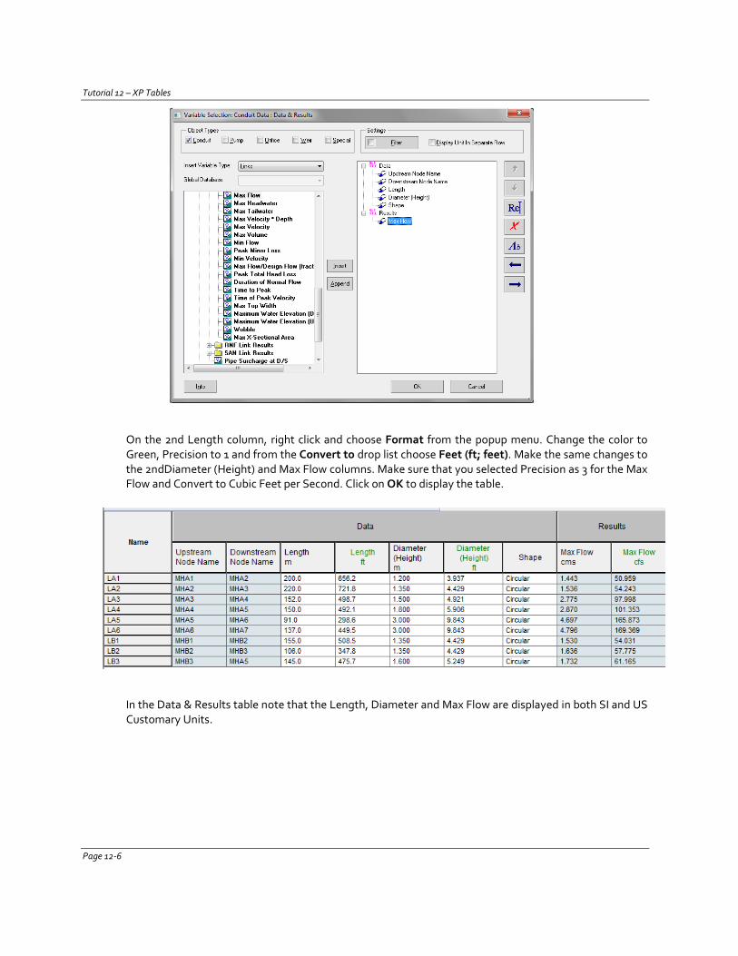
Tutorial 12 – XP Tables
On the 2nd Length column, right click and choose Format from the popup menu. Change the color to Green, Precision to 1 and from the Convert to drop list choose Feet (ft; feet). Make the same changes to the 2ndDiameter (Height) and Max Flow columns. Make sure that you selected Precision as 3 for the Max Flow and Convert to Cubic Feet per Second. Click on OK to display the table.
In the Data & Results table note that the Length, Diameter and Max Flow are displayed in both SI and US Customary Units.
Page 12-6
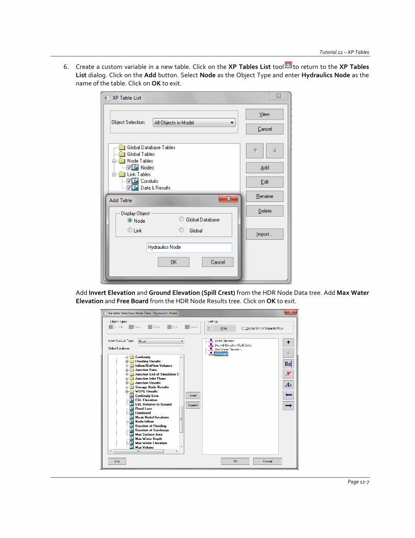
Tutorial 12 – XP Tables
6. Create a custom variable in a new table. Click on the XP Tables List tool to return to the XP Tables List dialog. Click on the Add button. Select Node as the Object Type and enter Hydraulics Node as the name of the table. Click on OK to exit.
Add Invert Elevation and Ground Elevation (Spill Crest) from the HDR Node Data tree. Add Max Water Elevation and Free Board from the HDR Node Results tree. Click on OK to exit.
Page 12-7
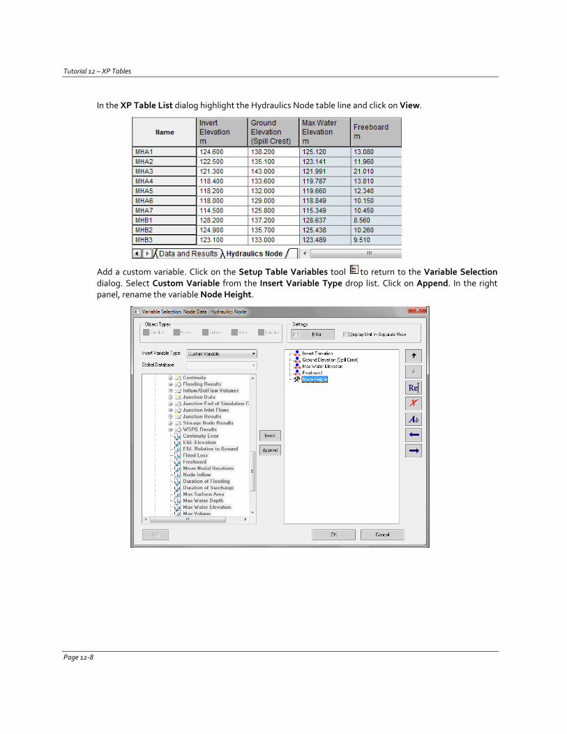
Tutorial 12 – XP Tables
In the XP Table List dialog highlight the Hydraulics Node table line and click on View.
Add a custom variable. Click on the Setup Table Variables tool to return to the Variable Selection dialog. Select Custom Variable from the Insert Variable Type drop list. Click on Append. In the right panel, rename the variable Node Height.
Page 12-8
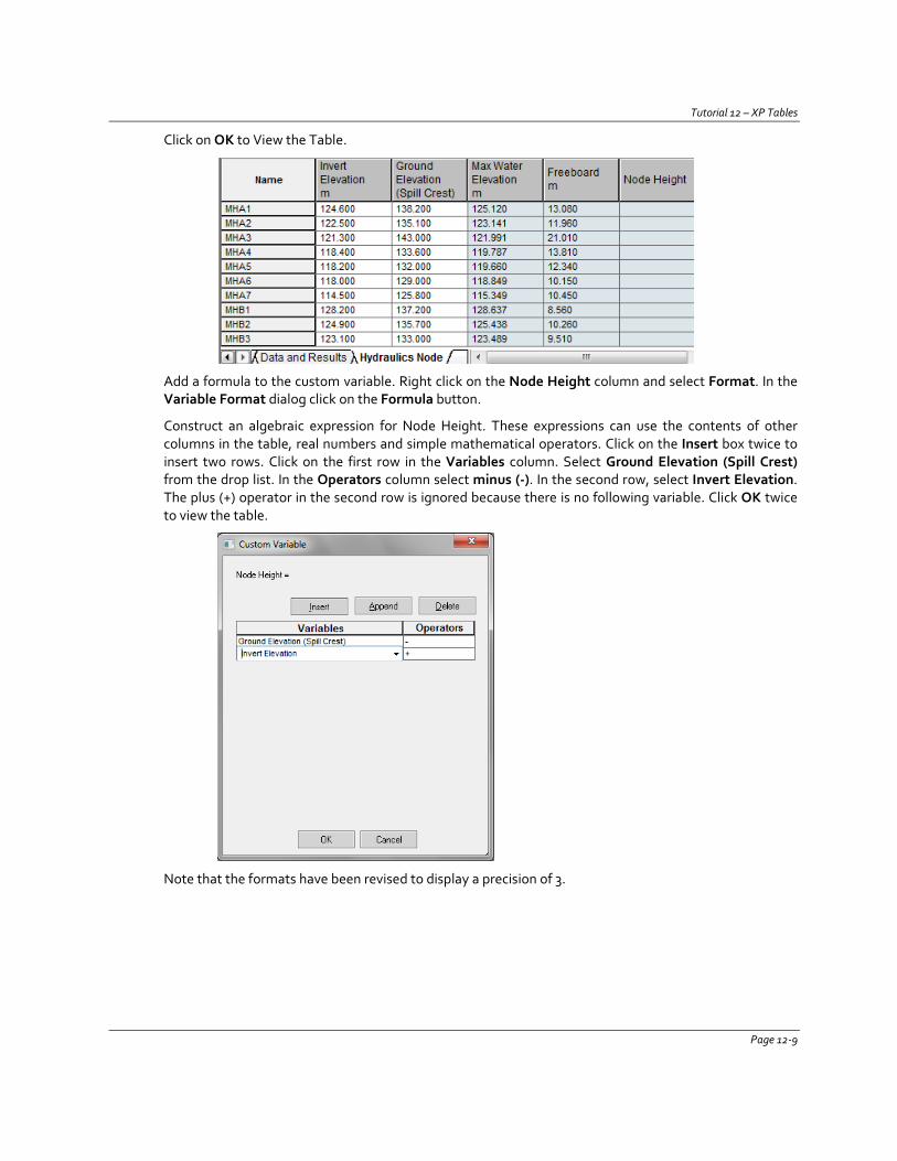
Tutorial 12 – XP Tables
Click on OK to View the Table.
Add a formula to the custom variable. Right click on the Node Height column and select Format. In the Variable Format dialog click on the Formula button.
Construct an algebraic expression for Node Height. These expressions can use the contents of other columns in the table, real numbers and simple mathematical operators. Click on the Insert box twice to insert two rows. Click on the first row in the Variables column. Select Ground Elevation (Spill Crest) from the drop list. In the Operators column select minus (-). In the second row, select Invert Elevation. The plus (+) operator in the second row is ignored because there is no following variable. Click OK twice to view the table.
Note that the formats have been revised to display a precision of 3.
Page 12-9
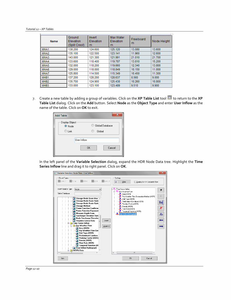
Tutorial 12 – XP Tables
7. Create a new table by adding a group of variables. Click on the XP Table List tool to return to the XP Table List dialog. Click on the Add button. Select Node as the Object Type and enter User Inflow as the name of the table. Click on OK to exit.
In the left panel of the Variable Selection dialog, expand the HDR Node Data tree. Highlight the Time Series Inflow line and drag it to right panel. Click on OK.
Page 12-10
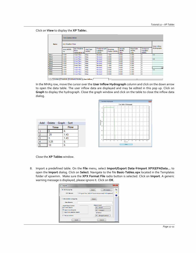
Tutorial 12 – XP Tables
Click on View to display the XP Tables.
In the MHA3 row, move the cursor over the User Inflow Hydrograph column and click on the down arrow to open the data table. The user inflow data are displayed and may be edited in this pop up. Click on Graph to display the hydrograph. Close the graph window and click on the table to close the inflow data dialog.
Close the XP Tables window.
8. Import a predefined table. On the File menu, select Import/Export DataImport XPX\EPAData… to open the Import dialog. Click on Select. Navigate to the file Basic-Tables.xpx located in the Templates folder of xpswmm. Make sure the XPX Format File radio button is selected. Click on Import. A generic warning message is displayed, please ignore it. Click on OK.
Page 12-11
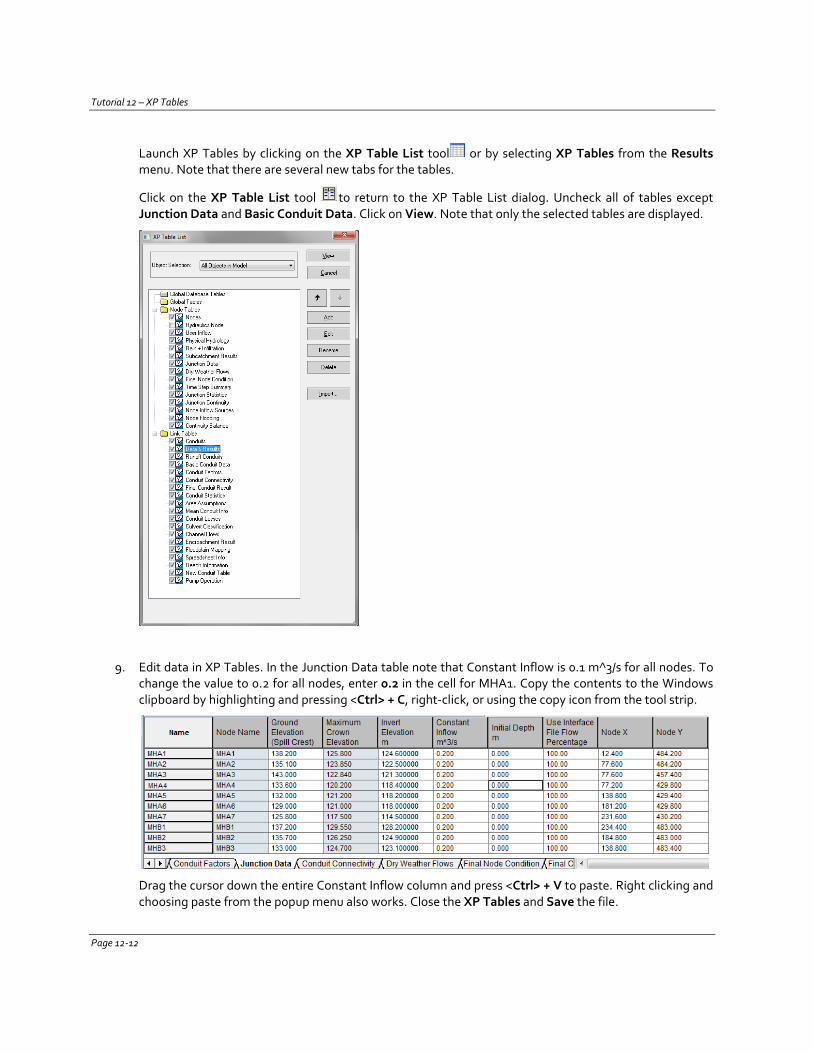
Tutorial 12 – XP Tables
Launch XP Tables by clicking on the XP Table List tool or by selecting XP Tables from the Results menu. Note that there are several new tabs for the tables.
Click on the XP Table List tool to return to the XP Table List dialog. Uncheck all of tables except Junction Data and Basic Conduit Data. Click on View. Note that only the selected tables are displayed.
9. Edit data in XP Tables. In the Junction Data table note that Constant Inflow is 0.1 m^3/s for all nodes. To change the value to 0.2 for all nodes, enter 0.2 in the cell for MHA1. Copy the contents to the Windows clipboard by highlighting and pressing <Ctrl> + C, right-click, or using the copy icon from the tool strip.
Drag the cursor down the entire Constant Inflow column and press <Ctrl> + V to paste. Right clicking and choosing paste from the popup menu also works. Close the XP Tables and Save the file.
Page 12-12
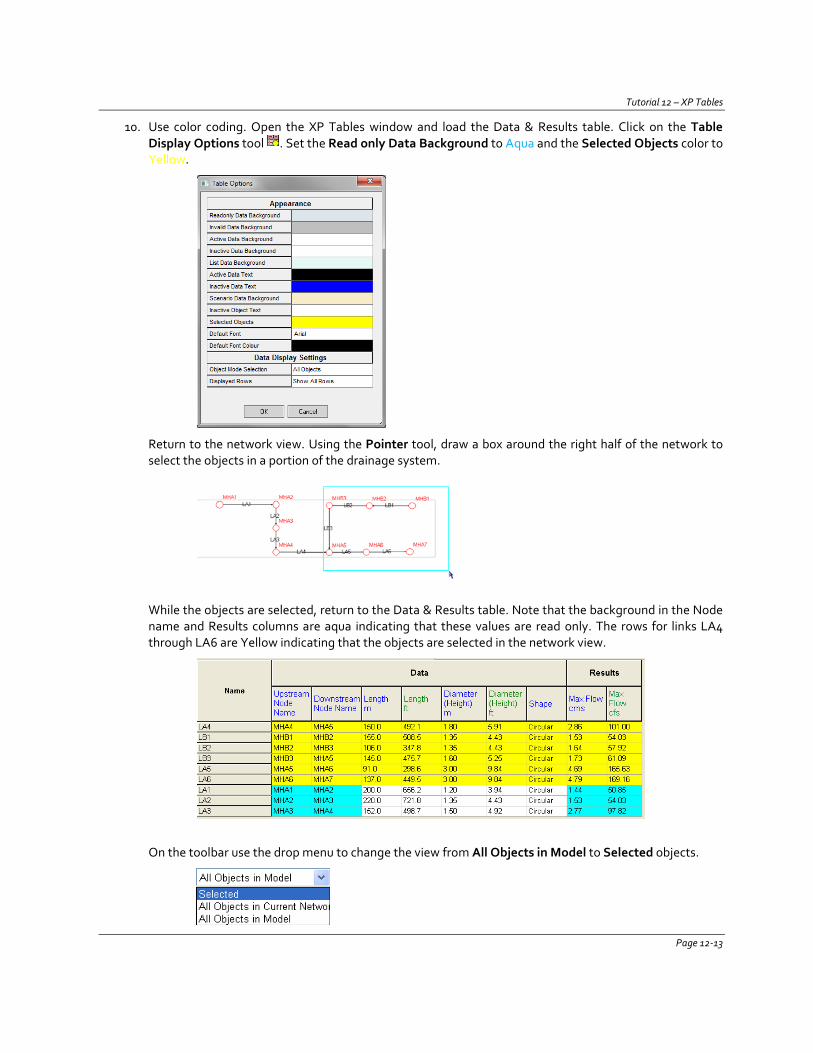
Tutorial 12 – XP Tables
10. Use color coding. Open the XP Tables window and load the Data & Results table. Click on the Table Display Options tool . Set the Read only Data Background to Aqua and the Selected Objects color to Yellow.
Return to the network view. Using the Pointer tool, draw a box around the right half of the network to select the objects in a portion of the drainage system.
While the objects are selected, return to the Data & Results table. Note that the background in the Node name and Results columns are aqua indicating that these values are read only. The rows for links LA4 through LA6 are Yellow indicating that the objects are selected in the network view.
On the toolbar use the drop menu to change the view from All Objects in Model to Selected objects.
Page 12-13
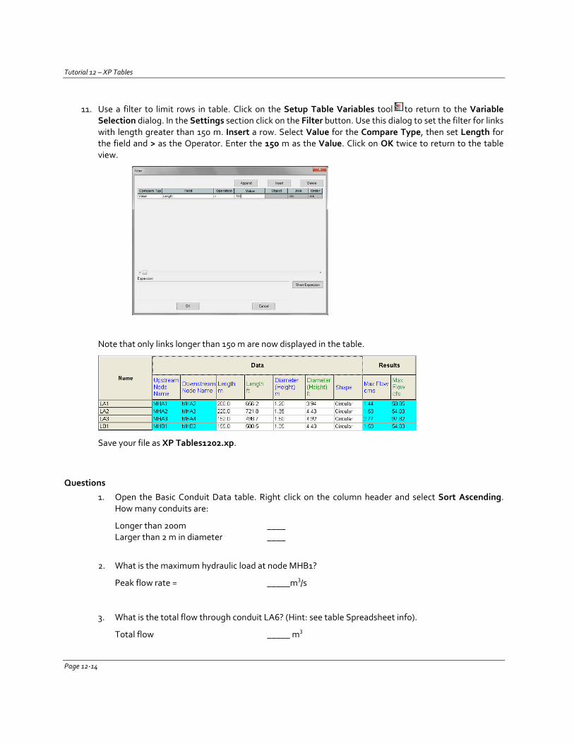
Tutorial 12 – XP Tables
11. Use a filter to limit rows in table. Click on the Setup Table Variables tool to return to the Variable Selection dialog. In the Settings section click on the Filter button. Use this dialog to set the filter for links with length greater than 150 m. Insert a row. Select Value for the Compare Type, then set Length for the field and > as the Operator. Enter the 150 m as the Value. Click on OK twice to return to the table view.
Note that only links longer than 150 m are now displayed in the table.
Save your file as XP Tables1202.xp.
Questions
1. Open the Basic Conduit Data table. Right click on the column header and select Sort Ascending. How many conduits are:
Longer than 200m ____ Larger than 2 m in diameter ____
2. What is the maximum hydraulic load at node MHB1?
Peak flow rate = _____m3/s 3. What is the total flow through conduit LA6? (Hint: see table Spreadsheet info).
Total flow _____ m3
Page 12-14
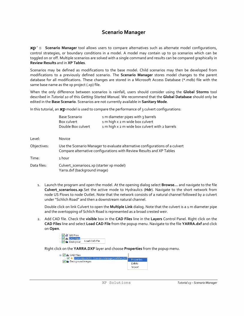
Scenario Manager
xp’s Scenario Manager tool allows users to compare alternatives such as alternate model configurations, control strategies, or boundary conditions in a model. A model may contain up to 50 scenarios which can be toggled on or off. Multiple scenarios are solved with a single command and results can be compared graphically in Review Results and in XP Tables.
Scenarios may be defined as modifications to the base model. Child scenarios may then be developed from modifications to a previously defined scenario. The Scenario Manager stores model changes to the parent database for all modifications. These changes are stored in a Microsoft Access Database (*.mdb) file with the same base name as the xp project (.xp) file.
When the only difference between scenarios is rainfall, users should consider using the Global Storms tool described in Tutorial 10 of this Getting Started Manual. We recommend that the Global Database should only be edited in the Base Scenario. Scenarios are not currently available in Sanitary Mode.
In this tutorial, an xp model is used to compare the performance of 3 culvert configurations:
Base Scenario 1 m diameter pipes with 3 barrels Box culvert 1 m high x 2 m wide box culvert Double Box culvert 1 m high x 2 m wide box culvert with 2 barrels
Level: Novice
Objectives: Use the Scenario Manager to evaluate alternative configurations of a culvert Compare alternative configurations with Review Results and XP Tables
Time: 1 hour
Data files: Culvert_scenario01.xp (starter xp model) Yarra.dxf (background image)
1. Launch the program and open the model. At the opening dialog select Browse… and navigate to the file Culvert_scenario01.xp.Set the active mode to Hydraulics (Hdr). Navigate to the short network from node US Flows to node Outlet. Note that the network consists of a natural channel followed by a culvert under “Schlich Road” and then a downstream natural channel.
Double click on link Culvert to open the Multiple Link dialog. Note that the culvert is a 1 m diameter pipe and the overtopping of Schlich Road is represented as a broad crested weir.
2. Add CAD file. Check the visible box in the CAD Files line in the Layers Control Panel. Right click on the CAD Files line and select Load CAD File from the popup menu. Navigate to the file YARRA.dxf and click on Open.
Right click on the YARRA.DXF layer and choose Properties from the popup menu.
XP Solutions Tutorial 13 – Scenario Manager
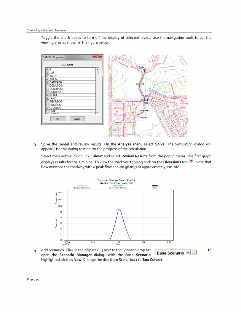
Tutorial 13 – Scenario Manager
Toggle the check boxes to turn off the display of selected layers. Use the navigation tools to set the viewing area as shown in the figure below:
3. Solve the model and review results. On the Analyze menu select Solve. The Simulation dialog will appear. Use this dialog to monitor the progress of the calculation.
Select then right-click on link Culvert and select Review Results from the popup menu. The first graph
displays results for the 1 m pipe. To view the road overtopping click on the Diversions tool . Note that flow overtops the roadway with a peak flow about0.56 m3/s at approximately 1:01 AM.
4. Add scenarios. Click in the ellipses (…) next to the Scenario drop list to open the Scenario Manager dialog. With the Base Scenario highlighted click on New. Change the title from Scenario#1 to Box Culvert.
Page 13-2
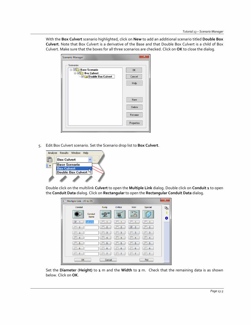
Tutorial 13 – Scenario Manager
With the Box Culvert scenario highlighted, click on New to add an additional scenario titled Double Box Culvert. Note that Box Culvert is a derivative of the Base and that Double Box Culvert is a child of Box Culvert. Make sure that the boxes for all three scenarios are checked. Click on OK to close the dialog.
5. Edit Box Culvert scenario. Set the Scenario drop list to Box Culvert.
Double click on the multilink Culvert to open the Multiple Link dialog. Double click on Conduit 1 to open the Conduit Data dialog. Click on Rectangular to open the Rectangular Conduit Data dialog.
Set the Diameter (Height) to 1 m and the Width to 2 m. Check that the remaining data is as shown below. Click on OK.
Page 13-3
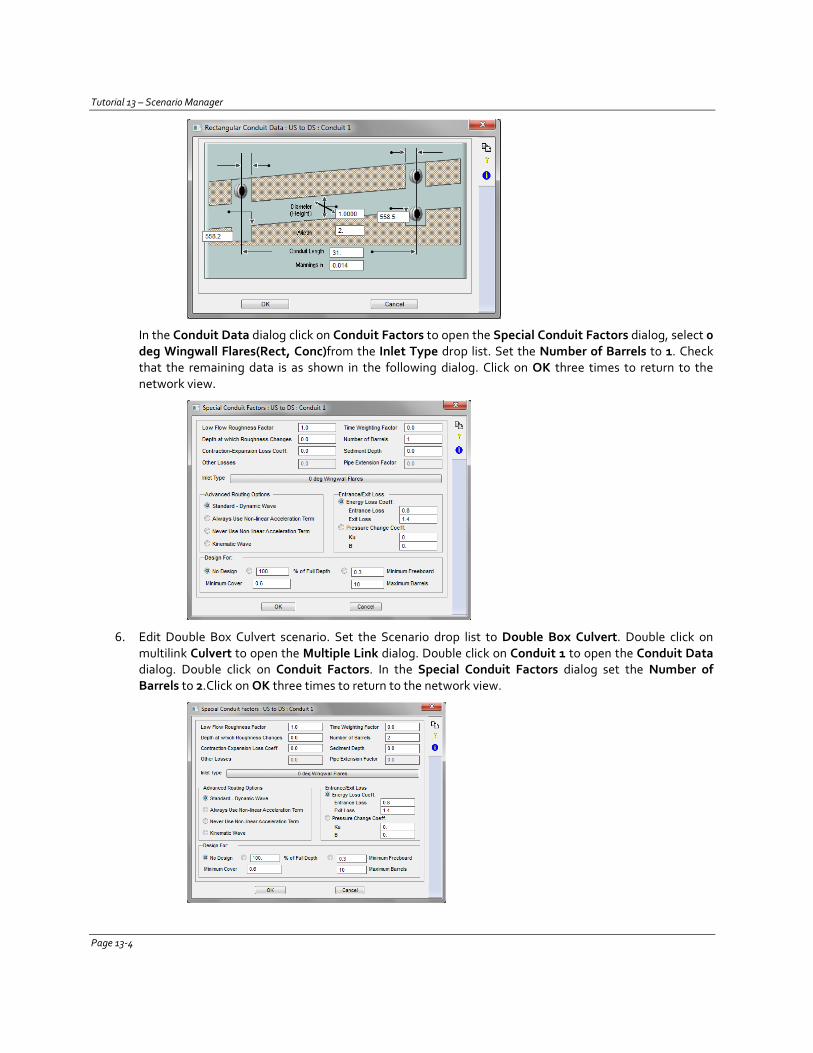
Tutorial 13 – Scenario Manager
In the Conduit Data dialog click on Conduit Factors to open the Special Conduit Factors dialog, select 0 deg Wingwall Flares(Rect, Conc)from the Inlet Type drop list. Set the Number of Barrels to 1. Check that the remaining data is as shown in the following dialog. Click on OK three times to return to the network view.
6. Edit Double Box Culvert scenario. Set the Scenario drop list to Double Box Culvert. Double click on multilink Culvert to open the Multiple Link dialog. Double click on Conduit 1 to open the Conduit Data dialog. Double click on Conduit Factors. In the Special Conduit Factors dialog set the Number of Barrels to 2.Click on OK three times to return to the network view.
Page 13-4
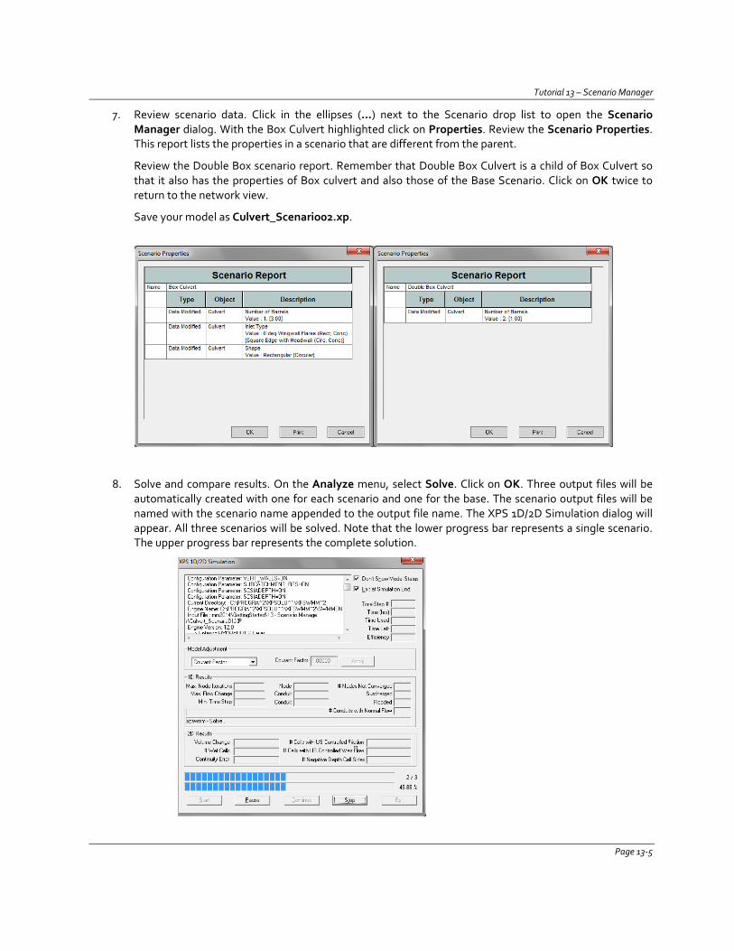
Tutorial 13 – Scenario Manager
7. Review scenario data. Click in the ellipses (…) next to the Scenario drop list to open the Scenario Manager dialog. With the Box Culvert highlighted click on Properties. Review the Scenario Properties. This report lists the properties in a scenario that are different from the parent.
Review the Double Box scenario report. Remember that Double Box Culvert is a child of Box Culvert so that it also has the properties of Box culvert and also those of the Base Scenario. Click on OK twice to return to the network view.
Save your model as Culvert_Scenario02.xp.
8. Solve and compare results. On the Analyze menu, select Solve. Click on OK. Three output files will be automatically created with one for each scenario and one for the base. The scenario output files will be named with the scenario name appended to the output file name. The XPS 1D/2D Simulation dialog will appear. All three scenarios will be solved. Note that the lower progress bar represents a single scenario. The upper progress bar represents the complete solution.
Page 13-5
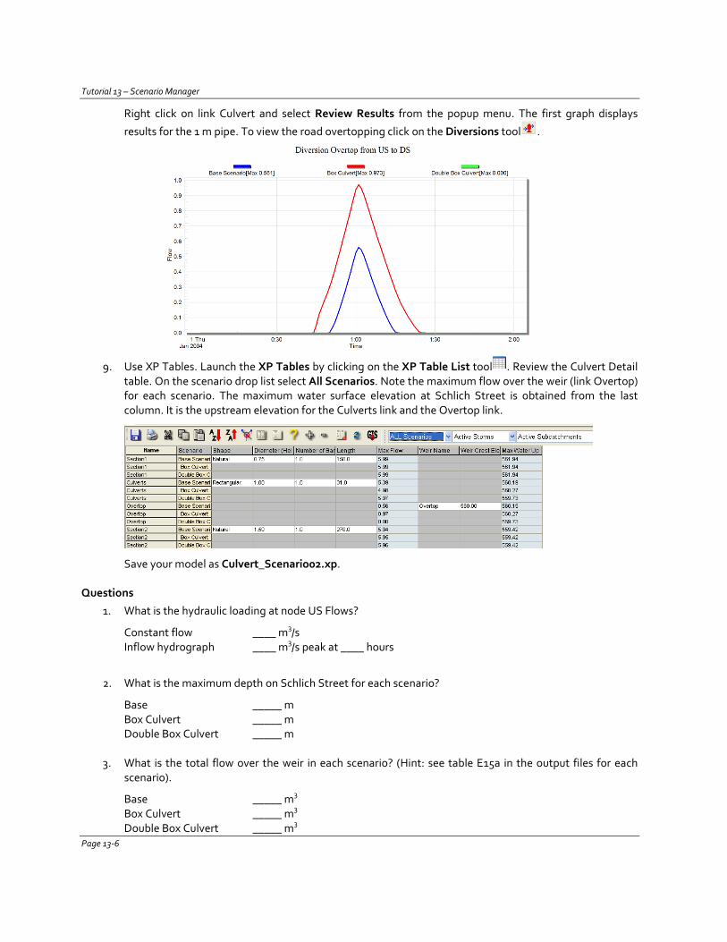
Tutorial 13 – Scenario Manager
Right click on link Culvert and select Review Results from the popup menu. The first graph displays
results for the 1 m pipe. To view the road overtopping click on the Diversions tool .
9. Use XP Tables. Launch the XP Tables by clicking on the XP Table List tool . Review the Culvert Detail table. On the scenario drop list select All Scenarios. Note the maximum flow over the weir (link Overtop) for each scenario. The maximum water surface elevation at Schlich Street is obtained from the last column. It is the upstream elevation for the Culverts link and the Overtop link.
Save your model as Culvert_Scenario02.xp.
Questions
1. What is the hydraulic loading at node US Flows?
Constant flow ____ m3/s Inflow hydrograph ____ m3/s peak at ____ hours
2. What is the maximum depth on Schlich Street for each scenario?
Base _____ m Box Culvert _____ m Double Box Culvert _____ m
3. What is the total flow over the weir in each scenario? (Hint: see table E15a in the output files for each scenario).
Base _____ m3 Box Culvert _____ m3 Double Box Culvert _____ m3
Page 13-6
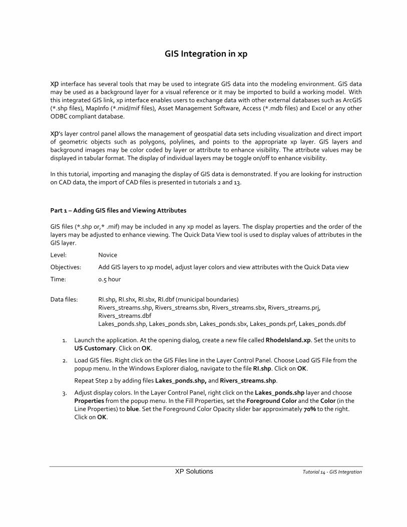
GIS Integration in xp
xp interface has several tools that may be used to integrate GIS data into the modeling environment. GIS data may be used as a background layer for a visual reference or it may be imported to build a working model. With this integrated GIS link, xp interface enables users to exchange data with other external databases such as ArcGIS (*.shp files), MapInfo (*.mid/mif files), Asset Management Software, Access (*.mdb files) and Excel or any other ODBC compliant database.
xp’s layer control panel allows the management of geospatial data sets including visualization and direct import of geometric objects such as polygons, polylines, and points to the appropriate xp layer. GIS layers and background images may be color coded by layer or attribute to enhance visibility. The attribute values may be displayed in tabular format. The display of individual layers may be toggle on/off to enhance visibility.
In this tutorial, importing and managing the display of GIS data is demonstrated. If you are looking for instruction on CAD data, the import of CAD files is presented in tutorials 2 and 13.
Part 1 – Adding GIS files and Viewing Attributes
GIS files (*.shp or,* .mif) may be included in any xp model as layers. The display properties and the order of the layers may be adjusted to enhance viewing. The Quick Data View tool is used to display values of attributes in the GIS layer.
Level: Novice
Objectives: Add GIS layers to xp model, adjust layer colors and view attributes with the Quick Data view
Time: 0.5 hour
Data files: RI.shp, RI.shx, RI.sbx, RI.dbf (municipal boundaries)
Rivers_streams.shp, Rivers_streams.sbn, Rivers_streams.sbx, Rivers_streams.prj, Rivers_streams.dbf Lakes_ponds.shp, Lakes_ponds.sbn, Lakes_ponds.sbx, Lakes_ponds.prf, Lakes_ponds.dbf
1. Launch the application. At the opening dialog, create a new file called RhodeIsland.xp. Set the units to
US Customary. Click on OK.
2. Load GIS files. Right click on the GIS Files line in the Layer Control Panel. Choose Load GIS File from the popup menu. In the Windows Explorer dialog, navigate to the file RI.shp. Click on OK.
Repeat Step 2 by adding files Lakes_ponds.shp, and Rivers_streams.shp.
3. Adjust display colors. In the Layer Control Panel, right click on the Lakes_ponds.shp layer and choose Properties from the popup menu. In the Fill Properties, set the Foreground Color and the Color (in the Line Properties) to blue. Set the Foreground Color Opacity slider bar approximately 70% to the right. Click on OK.
XP Solutions Tutorial 14 - GIS Integration

Tutorial 14 - GIS Integration
Right click on the Rivers_streams.shp layer and choose Properties from the popup menu. In the Fill Properties, set the Foreground Color and the Color (in the Line Properties) to light blue. Click on OK.
Right click on the RI.shp layer and choose Properties from the popup menu. In the Fill Properties, set the Foreground Color as White and the Color (in the Line Properties) to Black. Click on OK.
Adjust the network view to display the entire state of Rhode Island.
Page 14-2
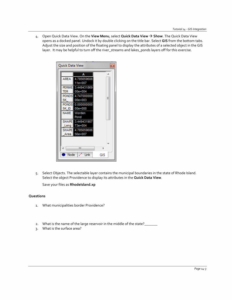
Tutorial 14 - GIS Integration
4. Open Quick Data View. On the View Menu, select Quick Data View Show. The Quick Data View opens as a docked panel. Undock it by double clicking on the title bar. Select GIS from the bottom tabs. Adjust the size and position of the floating panel to display the attributes of a selected object in the GIS layer. It may be helpful to turn off the river_streams and lakes_ponds layers off for this exercise.
5. Select Objects. The selectable layer contains the municipal boundaries in the state of Rhode Island. Select the object Providence to display its attributes in the Quick Data View.
Save your files as RhodeIsland.xp
Questions
1. What municipalities border Providence?
2. What is the name of the large reservoir in the middle of the state?_______ 3. What is the surface area?
Page 14-3
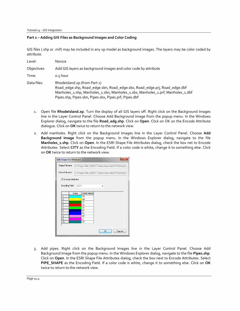
Tutorial 14 - GIS Integration
Part 2 – Adding GIS Files as Background Images and Color Coding
GIS files (.shp or .mif) may be included in any xp model as background images. The layers may be color coded by attribute.
Level: Novice
Objectives: Add GIS layers as background images and color code by attribute
Time: 0.5 hour
Data files: RhodeIsland.xp (from Part 1) Road_edge.shp, Road_edge.sbn, Road_edge.sbx, Road_edge.prj, Road_edge.dbf Manholes_1.shp, Manholes_1.sbn, Manholes_1.sbx, Manholes_1.prf, Manholes_1.dbf Pipes.shp, Pipes.sbn, Pipes.sbx, Pipes.prf, Pipes.dbf
1. Open file RhodeIsland.xp. Turn the display of all GIS layers off. Right click on the Background Images
line in the Layer Control Panel. Choose Add Background Image from the popup menu. In the Windows Explorer dialog, navigate to the file Road_edg.shp. Click on Open. Click on OK on the Encode Attribute dialogue. Click on OK twice to return to the network view.
2. Add manholes. Right click on the Background Images line in the Layer Control Panel. Choose Add Background Image from the popup menu. In the Windows Explorer dialog, navigate to the file Manholes_1.shp. Click on Open. In the ESRI Shape File Attributes dialog, check the box net to Encode Attributes. Select CITY as the Encoding Field. If a color code is white, change it to something else. Click on OK twice to return to the network view.
3. Add pipes. Right click on the Background Images line in the Layer Control Panel. Choose Add Background Image from the popup menu. In the Windows Explorer dialog, navigate to the file Pipes.shp. Click on Open. In the ESRI Shape File Attributes dialog, check the box next to Encode Attributes. Select PIPE_SHAPE as the Encoding Field. If a color code is white, change it to something else. Click on OK twice to return to the network view.
Page 14-4
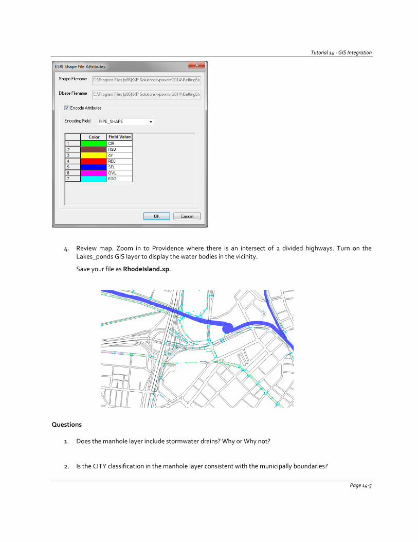
Tutorial 14 - GIS Integration
4. Review map. Zoom in to Providence where there is an intersect of 2 divided highways. Turn on the Lakes_ponds GIS layer to display the water bodies in the vicinity.
Save your file as RhodeIsland.xp.
Questions
1. Does the manhole layer include stormwater drains? Why or Why not?
2. Is the CITY classification in the manhole layer consistent with the municipally boundaries?
Page 14-5
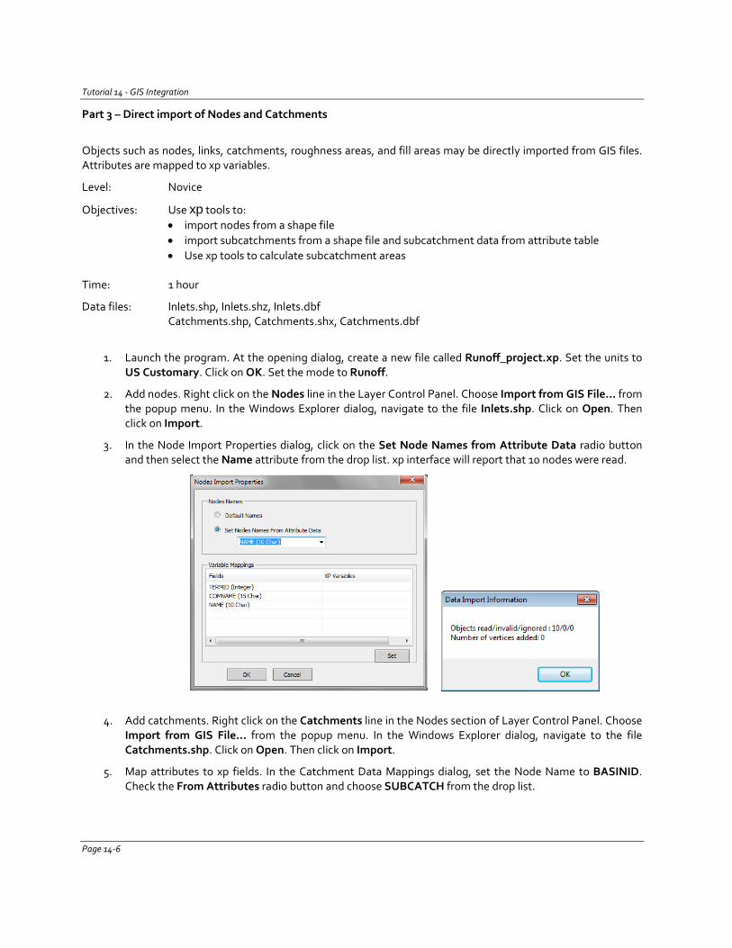
Tutorial 14 - GIS Integration
Part 3 – Direct import of Nodes and Catchments
Objects such as nodes, links, catchments, roughness areas, and fill areas may be directly imported from GIS files. Attributes are mapped to xp variables.
Level: Novice
Objectives: Use xp tools to: • import nodes from a shape file • import subcatchments from a shape file and subcatchment data from attribute table • Use xp tools to calculate subcatchment areas
Time: 1 hour
Data files: Inlets.shp, Inlets.shz, Inlets.dbf Catchments.shp, Catchments.shx, Catchments.dbf
1. Launch the program. At the opening dialog, create a new file called Runoff_project.xp. Set the units to US Customary. Click on OK. Set the mode to Runoff.
2. Add nodes. Right click on the Nodes line in the Layer Control Panel. Choose Import from GIS File… from the popup menu. In the Windows Explorer dialog, navigate to the file Inlets.shp. Click on Open. Then click on Import.
3. In the Node Import Properties dialog, click on the Set Node Names from Attribute Data radio button and then select the Name attribute from the drop list. xp interface will report that 10 nodes were read.
4. Add catchments. Right click on the Catchments line in the Nodes section of Layer Control Panel. Choose Import from GIS File… from the popup menu. In the Windows Explorer dialog, navigate to the file Catchments.shp. Click on Open. Then click on Import.
5. Map attributes to xp fields. In the Catchment Data Mappings dialog, set the Node Name to BASINID. Check the From Attributes radio button and choose SUBCATCH from the drop list.
Page 14-6
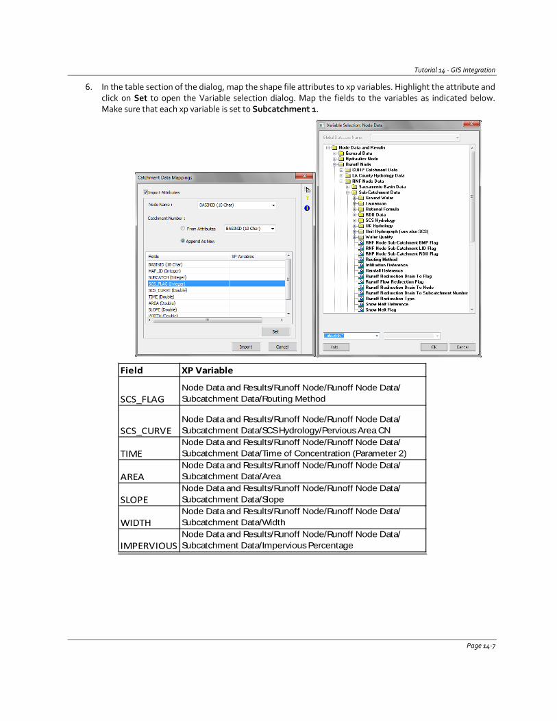
Tutorial 14 - GIS Integration
6. In the table section of the dialog, map the shape file attributes to xp variables. Highlight the attribute and click on Set to open the Variable selection dialog. Map the fields to the variables as indicated below. Make sure that each xp variable is set to Subcatchment 1.
Field XP Variable
SCS_FLAGNode Data and Results/Runoff Node/Runoff Node Data/ Subcatchment Data/Routing Method
SCS_CURVENode Data and Results/Runoff Node/Runoff Node Data/ Subcatchment Data/SCS Hydrology/Pervious Area CN
TIMENode Data and Results/Runoff Node/Runoff Node Data/ Subcatchment Data/Time of Concentration (Parameter 2)
AREANode Data and Results/Runoff Node/Runoff Node Data/ Subcatchment Data/Area
SLOPENode Data and Results/Runoff Node/Runoff Node Data/ Subcatchment Data/Slope
WIDTHNode Data and Results/Runoff Node/Runoff Node Data/ Subcatchment Data/Width
IMPERVIOUSNode Data and Results/Runoff Node/Runoff Node Data/ Subcatchment Data/Impervious Percentage
Page 14-7
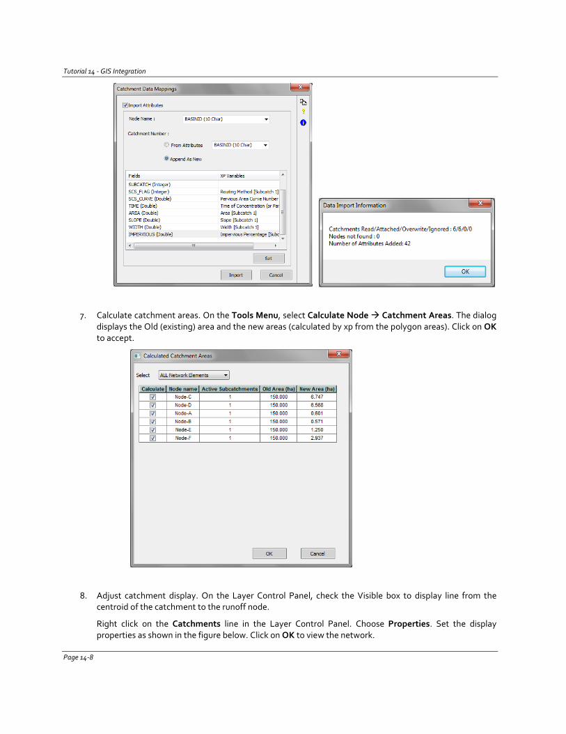
Tutorial 14 - GIS Integration
7. Calculate catchment areas. On the Tools Menu, select Calculate Node Catchment Areas. The dialog displays the Old (existing) area and the new areas (calculated by xp from the polygon areas). Click on OK to accept.
8. Adjust catchment display. On the Layer Control Panel, check the Visible box to display line from the centroid of the catchment to the runoff node.
Right click on the Catchments line in the Layer Control Panel. Choose Properties. Set the display properties as shown in the figure below. Click on OK to view the network.
Page 14-8
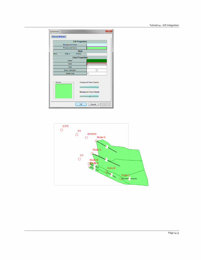
Tutorial 14 - GIS Integration
Page 14-9

Tutorial 14 - GIS Integration
Questions
1. Review the SCS Hydrology data for Node-A. How were the Hydrograph Shape and Initial Abstraction values entered into the model?
2. Use the ruler tool to measure the width of the catchment for Node-E. _____ft.
Page 14-10
DTM and River Modeling
River models employ the same link-node scheme that is used for pipe networks. In river models links are typically trapezoidal or natural cross sections representing river reaches. The cross sections representing each reach can be developed from topographic data.
The xp interface has tools for automating the process of constructing a river model from topographic data. Invert elevations, cross section shapes and conduit lengths may all be obtained and adjusted in the user interface.
In order to access topographic data it must be in the form of digital terrain model (DTM). xp interface uses a Triangular Irregular Network (TIN) format. The data are stored in file with name filename.xptin. An embedded tool in the software will generate the DTM from x, y, z data.
In this tutorial a 1-dimensionsal hydraulic model of river is created using a background image for the layout and a DTM to assign required elevations.
Part 1 – Adding a Background Image and Creating a DTM
Georeferenced image files (.bmp, .jpg, .tif, .ecw, .sid and others) are used as background images to layout a network. A DTM is created from survey data and used to assign inverts and create shapes of cross sections for a river model.
Level: Novice
Objectives: Add a background image to an xp model Create a digital terrain model (DTM) from survey data Adjust the display of the DTM Use DTM to cut cross sections Time: 0.5 hour
Data files: River site.tif (background image file) River_siteUS.txt (topographic data in text format)
1. Launch the program. At the opening dialog create a new file called DTM_and_River.xp. Set the units to US Customary. Click on OK.
2. Load background image file. Right click on the Background Images line in the Layer Control Panel. Choose Add Background Image from the popup menu. In the Windows Explorer dialog navigate to the file River site.tif. Click on Open.
Note that the coordinates of the Destination Rectangle are filled in from the coordinates listed in the image *.tlf file. Click on OK.
Explore the image with the mouse. Note that the x and y coordinates are displayed in the status bar at the bottom of the network window. Use the mouse wheel to zone in and out. Right click and the cursor
will display the hand (Pan Tool). Use the hand to drag the image around the network viewing panel.
XP Solutions Tutorial 15 - DTM and River Modeling
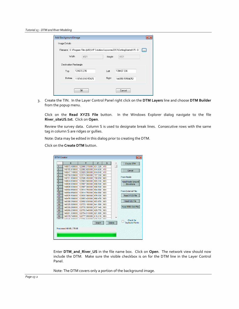
Tutorial 15 - DTM and River Modeling
3. Create the TIN. In the Layer Control Panel right click on the DTM Layers line and choose DTM Builder from the popup menu.
Click on the Read XYZS File button. In the Windows Explorer dialog navigate to the file River_siteUS.txt. Click on Open.
Review the survey data. Column S is used to designate break lines. Consecutive rows with the same tag in column S are ridges or gullies.
Note: Data may be edited in this dialog prior to creating the DTM.
Click on the Create DTM button.
Enter DTM_and_River_US in the file name box. Click on Open. The network view should now include the DTM. Make sure the visible checkbox is on for the DTM line in the Layer Control Panel. Note: The DTM covers only a portion of the background image.
Page 15-2
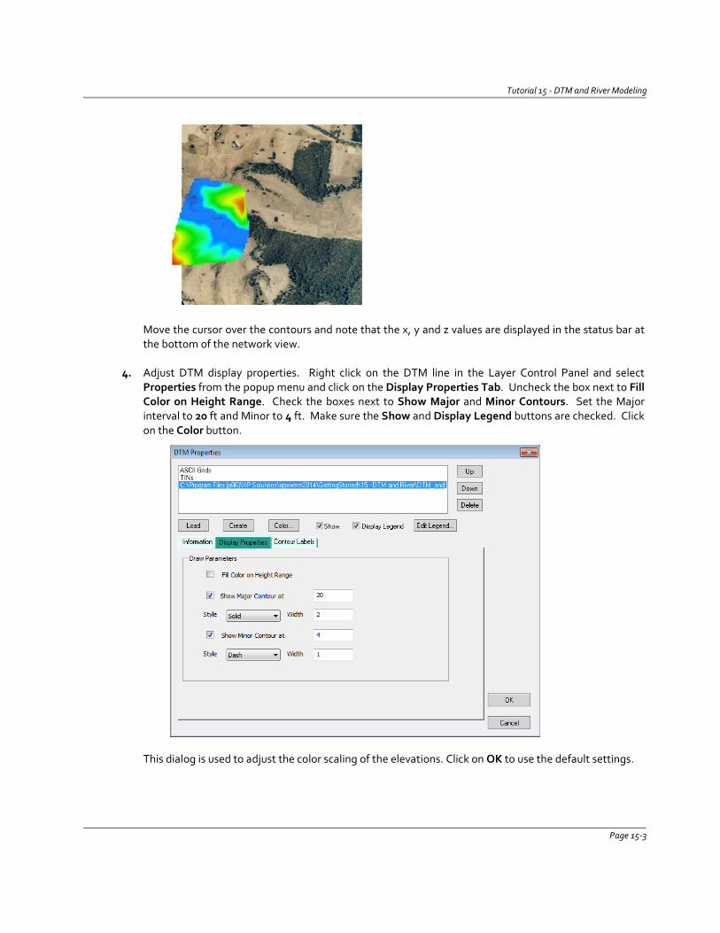
Tutorial 15 - DTM and River Modeling
Move the cursor over the contours and note that the x, y and z values are displayed in the status bar at the bottom of the network view.
4. Adjust DTM display properties. Right click on the DTM line in the Layer Control Panel and select
Properties from the popup menu and click on the Display Properties Tab. Uncheck the box next to Fill Color on Height Range. Check the boxes next to Show Major and Minor Contours. Set the Major interval to 20 ft and Minor to 4 ft. Make sure the Show and Display Legend buttons are checked. Click on the Color button.
This dialog is used to adjust the color scaling of the elevations. Click on OK to use the default settings.
Page 15-3
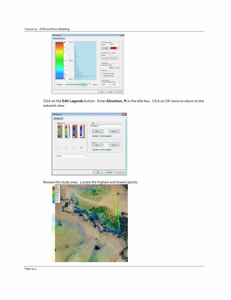
Tutorial 15 - DTM and River Modeling
Click on the Edit Legends button. Enter Elevation, ft in the title box. Click on OK twice to return to the network view.
Review the study area. Locate the highest and lowest points.
Page 15-4
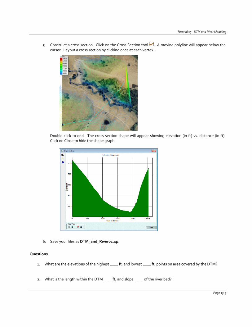
Tutorial 15 - DTM and River Modeling
5. Construct a cross section. Click on the Cross Section tool . A moving polyline will appear below the
cursor. Layout a cross section by clicking once at each vertex.
Double click to end. The cross section shape will appear showing elevation (in ft) vs. distance (in ft). Click on Close to hide the shape graph.
6. Save your files as DTM_and_River01.xp.
Questions
1. What are the elevations of the highest ____ ft, and lowest ____ ft, points on area covered by the DTM? 2. What is the length within the DTM ____ ft, and slope ____ of the river bed?
Page 15-5
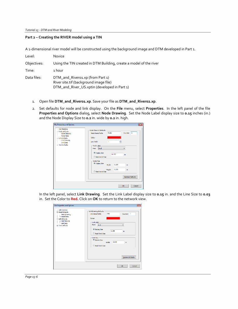
Tutorial 15 - DTM and River Modeling
Part 2 – Creating the RIVER model using a TIN
A 1-dimensional river model will be constructed using the background image and DTM developed in Part 1.
Level: Novice
Objectives: Using the TIN created in DTM Building, create a model of the river
Time: 1 hour
Data files: DTM_and_River01.xp (from Part 1) River site.tif (background image file)
DTM_and_River_US.xptin (developed in Part 1)
1. Open file DTM_and_River01.xp. Save your file as DTM_and_River02.xp.
2. Set defaults for node and link display. On the File menu, select Properties. In the left panel of the file Properties and Options dialog, select Node Drawing. Set the Node Label display size to 0.15 inches (in.) and the Node Display Size to 0.2 in. wide by 0.2 in. high.
In the left panel, select Link Drawing. Set the Link Label display size to 0.15 in. and the Line Size to 0.03 in. Set the Color to Red. Click on OK to return to the network view.
Page 15-6
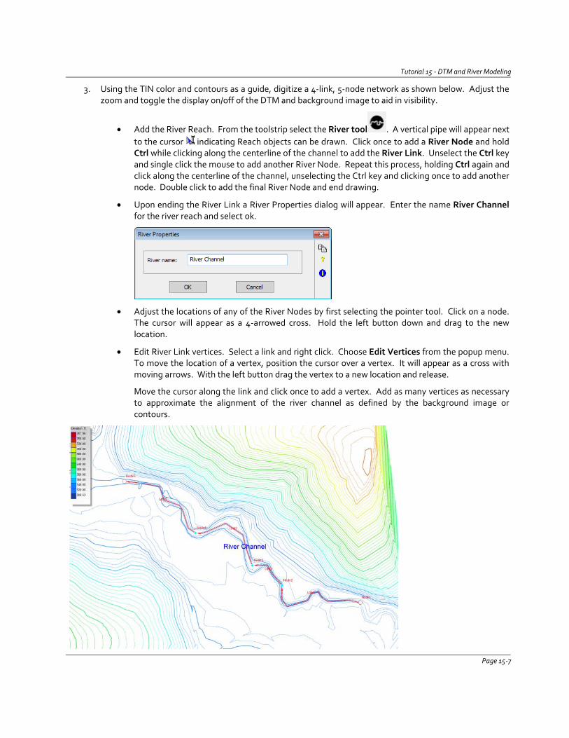
Tutorial 15 - DTM and River Modeling
3. Using the TIN color and contours as a guide, digitize a 4-link, 5-node network as shown below. Adjust the zoom and toggle the display on/off of the DTM and background image to aid in visibility.
• Add the River Reach. From the toolstrip select the River tool . A vertical pipe will appear next to the cursor indicating Reach objects can be drawn. Click once to add a River Node and hold Ctrl while clicking along the centerline of the channel to add the River Link. Unselect the Ctrl key and single click the mouse to add another River Node. Repeat this process, holding Ctrl again and click along the centerline of the channel, unselecting the Ctrl key and clicking once to add another node. Double click to add the final River Node and end drawing.
• Upon ending the River Link a River Properties dialog will appear. Enter the name River Channel for the river reach and select ok.
• Adjust the locations of any of the River Nodes by first selecting the pointer tool. Click on a node. The cursor will appear as a 4-arrowed cross. Hold the left button down and drag to the new location.
• Edit River Link vertices. Select a link and right click. Choose Edit Vertices from the popup menu. To move the location of a vertex, position the cursor over a vertex. It will appear as a cross with moving arrows. With the left button drag the vertex to a new location and release.
Move the cursor along the link and click once to add a vertex. Add as many vertices as necessary to approximate the alignment of the river channel as defined by the background image or contours.
Page 15-7
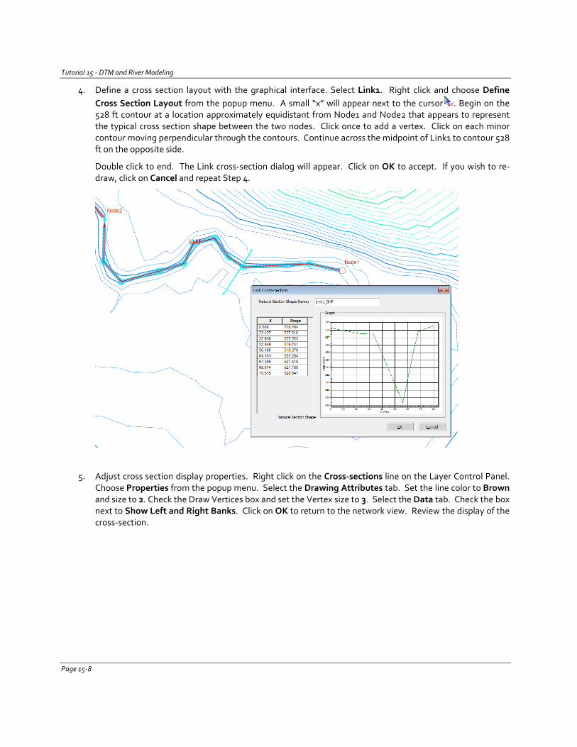
Tutorial 15 - DTM and River Modeling
4. Define a cross section layout with the graphical interface. Select Link1. Right click and choose Define Cross Section Layout from the popup menu. A small “x” will appear next to the cursor . Begin on the 528 ft contour at a location approximately equidistant from Node1 and Node2 that appears to represent the typical cross section shape between the two nodes. Click once to add a vertex. Click on each minor contour moving perpendicular through the contours. Continue across the midpoint of Link1 to contour 528 ft on the opposite side.
Double click to end. The Link cross-section dialog will appear. Click on OK to accept. If you wish to re-draw, click on Cancel and repeat Step 4.
5. Adjust cross section display properties. Right click on the Cross-sections line on the Layer Control Panel. Choose Properties from the popup menu. Select the Drawing Attributes tab. Set the line color to Brown and size to 2. Check the Draw Vertices box and set the Vertex size to 3. Select the Data tab. Check the box next to Show Left and Right Banks. Click on OK to return to the network view. Review the display of the cross-section.
Page 15-8
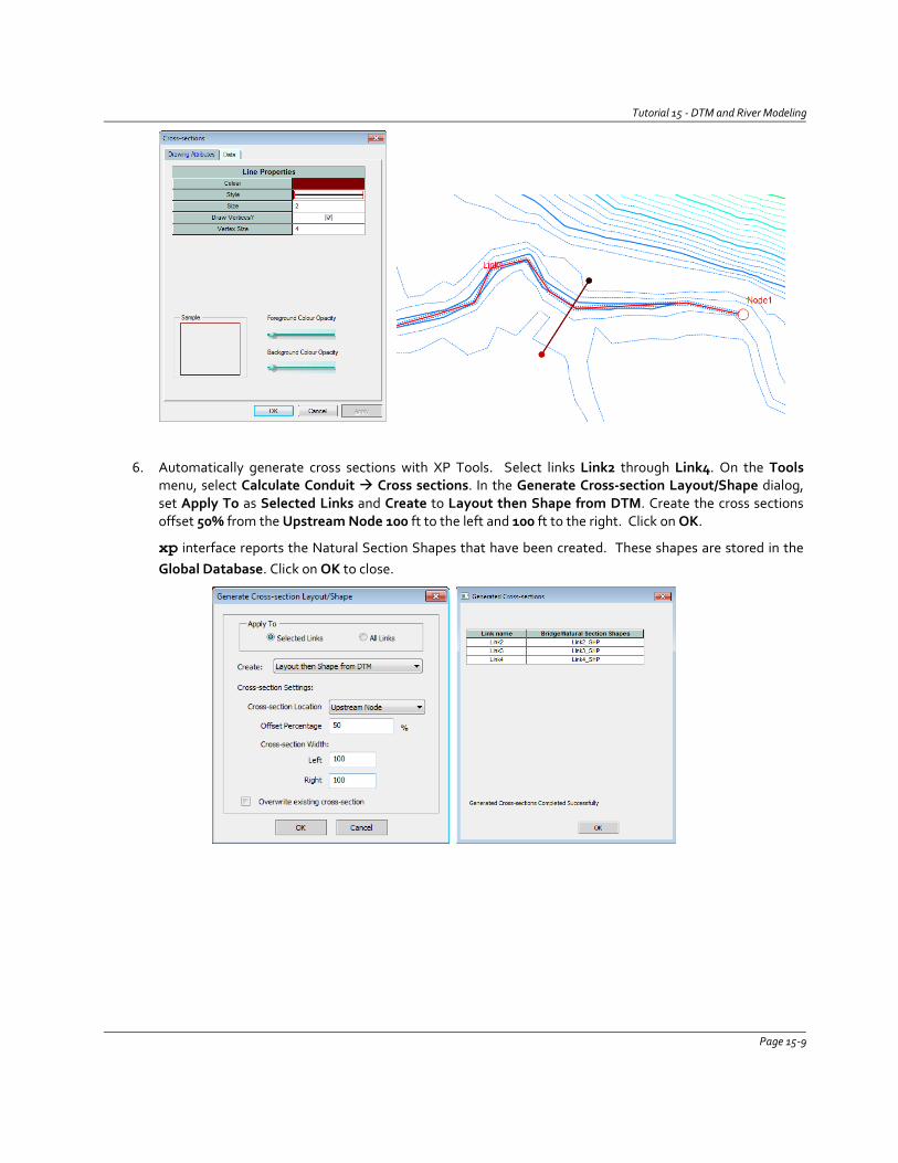
Tutorial 15 - DTM and River Modeling
6. Automatically generate cross sections with XP Tools. Select links Link2 through Link4. On the Tools menu, select Calculate Conduit Cross sections. In the Generate Cross-section Layout/Shape dialog, set Apply To as Selected Links and Create to Layout then Shape from DTM. Create the cross sections offset 50% from the Upstream Node 100 ft to the left and 100 ft to the right. Click on OK.
xp interface reports the Natural Section Shapes that have been created. These shapes are stored in the Global Database. Click on OK to close.
Page 15-9
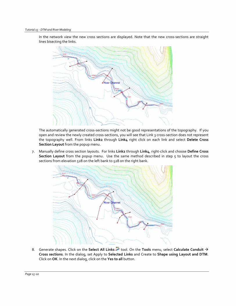
Tutorial 15 - DTM and River Modeling
In the network view the new cross sections are displayed. Note that the new cross-sections are straight lines bisecting the links.
The automatically generated cross-sections might not be good representations of the topography. If you open and review the newly created cross-sections, you will see that Link 3 cross-section does not represent the topography well. From links Link2 through Link4 right click on each link and select Delete Cross Section Layout from the popup menu.
7. Manually define cross section layouts. For links Link2 through Link4, right-click and choose Define Cross Section Layout from the popup menu. Use the same method described in step 5 to layout the cross sections from elevation 528 on the left bank to 528 on the right bank.
8. Generate shapes. Click on the Select All Links tool. On the Tools menu, select Calculate Conduit Cross sections. In the dialog, set Apply to Selected Links and Create to Shape using Layout and DTM. Click on OK. In the next dialog, click on the Yes to all button.
Page 15-10
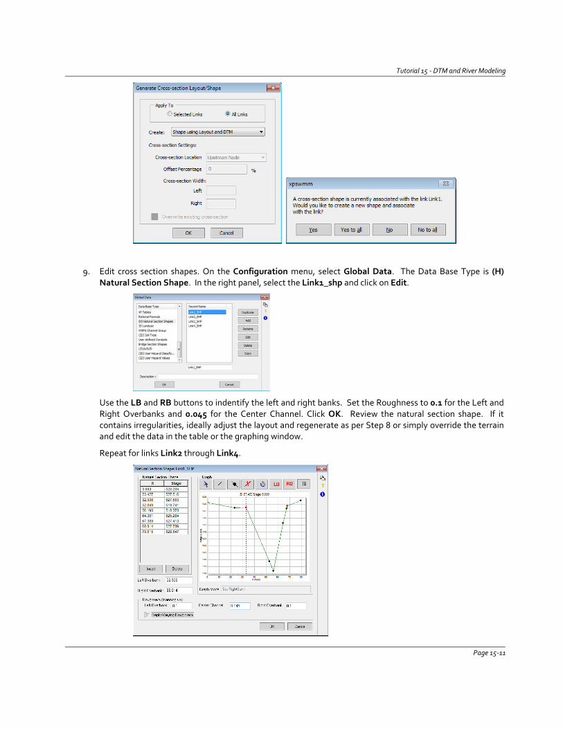
Tutorial 15 - DTM and River Modeling
9. Edit cross section shapes. On the Configuration menu, select Global Data. The Data Base Type is (H) Natural Section Shape. In the right panel, select the Link1_shp and click on Edit.
Use the LB and RB buttons to indentify the left and right banks. Set the Roughness to 0.1 for the Left and Right Overbanks and 0.045 for the Center Channel. Click OK. Review the natural section shape. If it contains irregularities, ideally adjust the layout and regenerate as per Step 8 or simply override the terrain and edit the data in the table or the graphing window.
Repeat for links Link2 through Link4.
Page 15-11
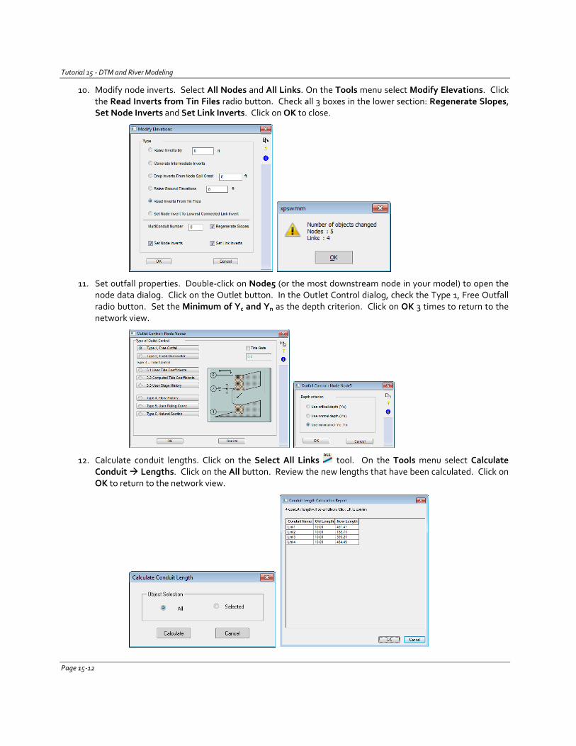
Tutorial 15 - DTM and River Modeling
10. Modify node inverts. Select All Nodes and All Links. On the Tools menu select Modify Elevations. Click the Read Inverts from Tin Files radio button. Check all 3 boxes in the lower section: Regenerate Slopes, Set Node Inverts and Set Link Inverts. Click on OK to close.
11. Set outfall properties. Double-click on Node5 (or the most downstream node in your model) to open the node data dialog. Click on the Outlet button. In the Outlet Control dialog, check the Type 1, Free Outfall radio button. Set the Minimum of Yc and Yn as the depth criterion. Click on OK 3 times to return to the network view.
12. Calculate conduit lengths. Click on the Select All Links tool. On the Tools menu select Calculate Conduit Lengths. Click on the All button. Review the new lengths that have been calculated. Click on OK to return to the network view.
Page 15-12

Tutorial 15 - DTM and River Modeling
On the Tools menu, select Calculate Conduit Slopes. Click on the All button. Review the new slopes that have been calculated. Click on OK to return to the network view.
13. Save your file as DTM and River 02.xp.
Questions
1. Use the Ruler tool to measure the straight line distance between Node1 and Node2. Compare the distance to the model length of Link1.
2. What is the impact of adding vertices to links on the hydraulic calculation?
3. Do the link slopes account for the elevation of the vertices?
Page 15-13
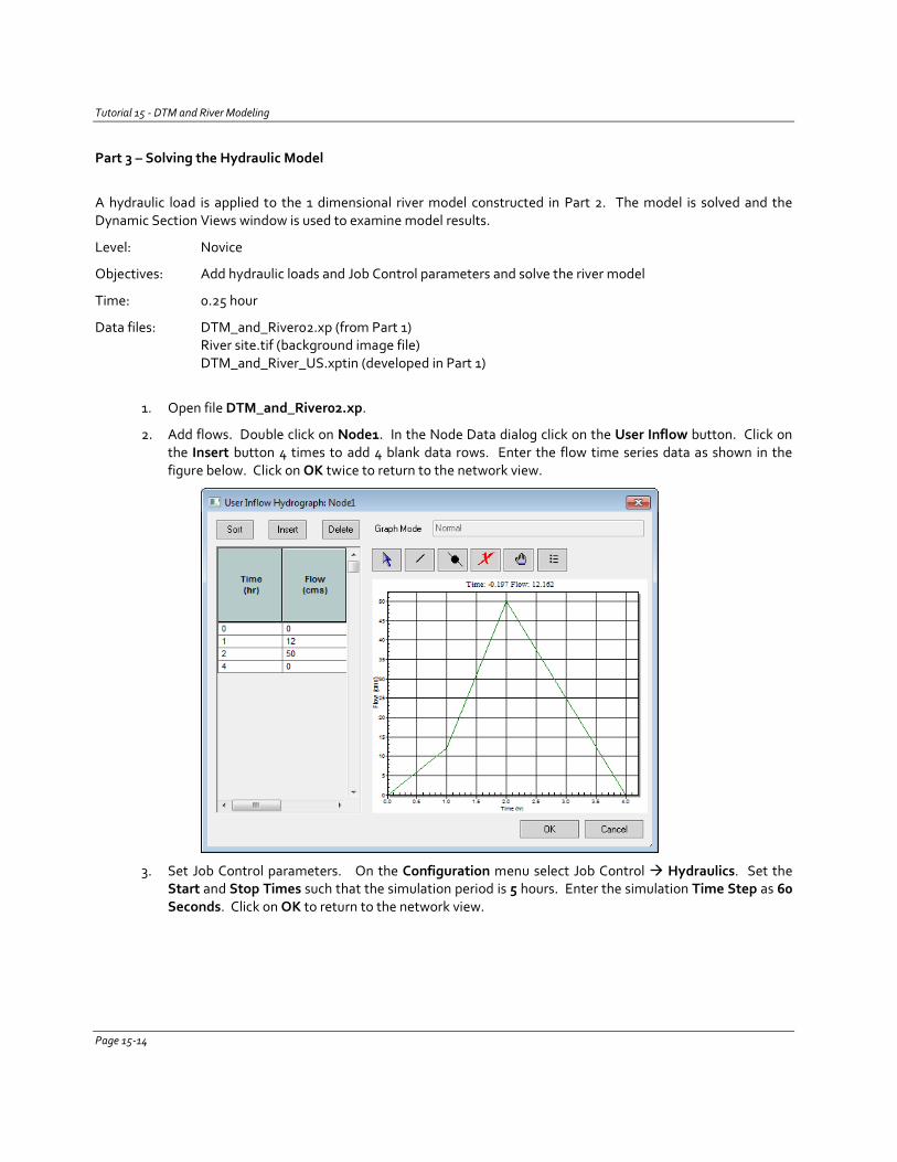
Tutorial 15 - DTM and River Modeling
Part 3 – Solving the Hydraulic Model
A hydraulic load is applied to the 1 dimensional river model constructed in Part 2. The model is solved and the Dynamic Section Views window is used to examine model results.
Level: Novice
Objectives: Add hydraulic loads and Job Control parameters and solve the river model
Time: 0.25 hour
Data files: DTM_and_River02.xp (from Part 1) River site.tif (background image file)
DTM_and_River_US.xptin (developed in Part 1)
1. Open file DTM_and_River02.xp.
2. Add flows. Double click on Node1. In the Node Data dialog click on the User Inflow button. Click on the Insert button 4 times to add 4 blank data rows. Enter the flow time series data as shown in the figure below. Click on OK twice to return to the network view.
3. Set Job Control parameters. On the Configuration menu select Job Control Hydraulics. Set the Start and Stop Times such that the simulation period is 5 hours. Enter the simulation Time Step as 60 Seconds. Click on OK to return to the network view.
Page 15-14
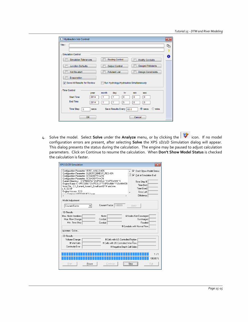
Tutorial 15 - DTM and River Modeling
4. Solve the model. Select Solve under the Analyze menu, or by clicking the icon. If no model configuration errors are present, after selecting Solve the XPS 1D/2D Simulation dialog will appear. This dialog presents the status during the calculation. The engine may be paused to adjust calculation parameters. Click on Continue to resume the calculation. When Don’t Show Model Status is checked the calculation is faster.
Page 15-15
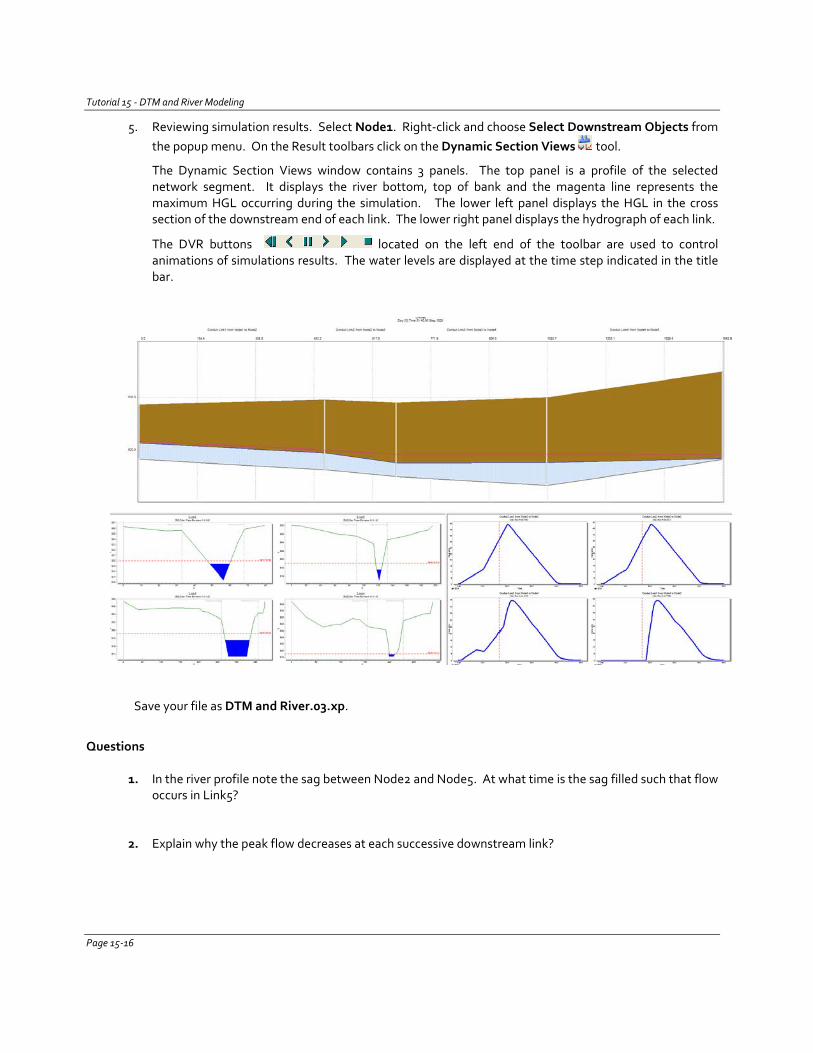
Tutorial 15 - DTM and River Modeling
5. Reviewing simulation results. Select Node1. Right-click and choose Select Downstream Objects from the popup menu. On the Result toolbars click on the Dynamic Section Views tool.
The Dynamic Section Views window contains 3 panels. The top panel is a profile of the selected network segment. It displays the river bottom, top of bank and the magenta line represents the maximum HGL occurring during the simulation. The lower left panel displays the HGL in the cross section of the downstream end of each link. The lower right panel displays the hydrograph of each link.
The DVR buttons located on the left end of the toolbar are used to control animations of simulations results. The water levels are displayed at the time step indicated in the title bar.
Save your file as DTM and River.03.xp.
Questions
1. In the river profile note the sag between Node2 and Node5. At what time is the sag filled such that flow occurs in Link5?
2. Explain why the peak flow decreases at each successive downstream link?
Page 15-16
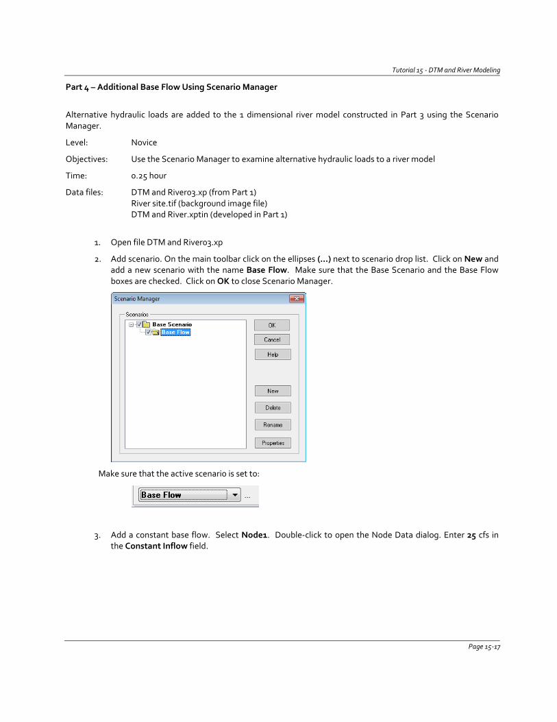
Tutorial 15 - DTM and River Modeling
Part 4 – Additional Base Flow Using Scenario Manager
Alternative hydraulic loads are added to the 1 dimensional river model constructed in Part 3 using the Scenario Manager.
Level: Novice
Objectives: Use the Scenario Manager to examine alternative hydraulic loads to a river model
Time: 0.25 hour
Data files: DTM and River03.xp (from Part 1) River site.tif (background image file)
DTM and River.xptin (developed in Part 1)
1. Open file DTM and River03.xp
2. Add scenario. On the main toolbar click on the ellipses (…) next to scenario drop list. Click on New and add a new scenario with the name Base Flow. Make sure that the Base Scenario and the Base Flow boxes are checked. Click on OK to close Scenario Manager.
Make sure that the active scenario is set to:
3. Add a constant base flow. Select Node1. Double-click to open the Node Data dialog. Enter 25 cfs in the Constant Inflow field.
Page 15-17
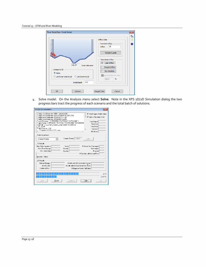
Tutorial 15 - DTM and River Modeling
4. Solve model. On the Analysis menu select Solve. Note in the XPS 1D/2D Simulation dialog the two progress bars tract the progress of each scenario and the total batch of solutions.
Page 15-18
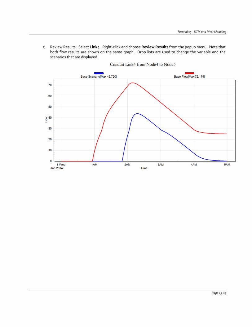
Tutorial 15 - DTM and River Modeling
5. Review Results. Select Link4. Right-click and choose Review Results from the popup menu. Note that both flow results are shown on the same graph. Drop lists are used to change the variable and the scenarios that are displayed.
Page 15-19
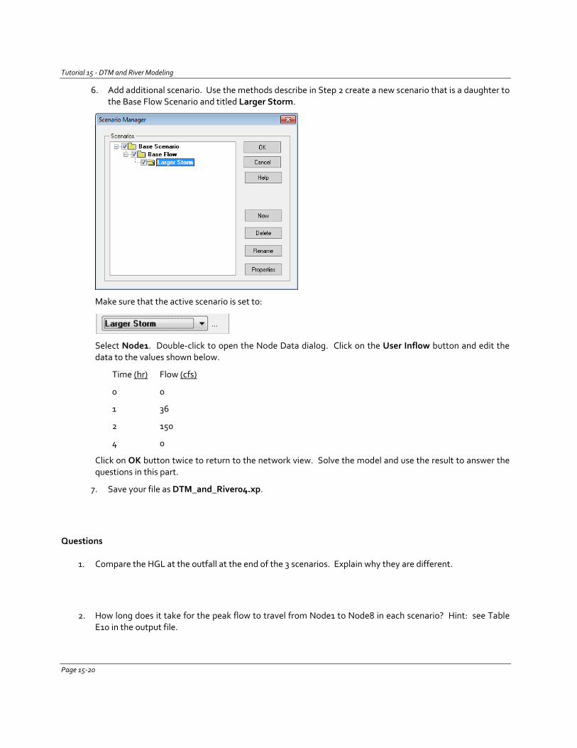
Tutorial 15 - DTM and River Modeling
6. Add additional scenario. Use the methods describe in Step 2 create a new scenario that is a daughter to the Base Flow Scenario and titled Larger Storm.
Make sure that the active scenario is set to:
Select Node1. Double-click to open the Node Data dialog. Click on the User Inflow button and edit the data to the values shown below.
Time (hr) Flow (cfs)
0 0
1 36
2 150
4 0
Click on OK button twice to return to the network view. Solve the model and use the result to answer the questions in this part.
7. Save your file as DTM_and_River04.xp.
Questions
1. Compare the HGL at the outfall at the end of the 3 scenarios. Explain why they are different.
2. How long does it take for the peak flow to travel from Node1 to Node8 in each scenario? Hint: see Table E10 in the output file.
Page 15-20
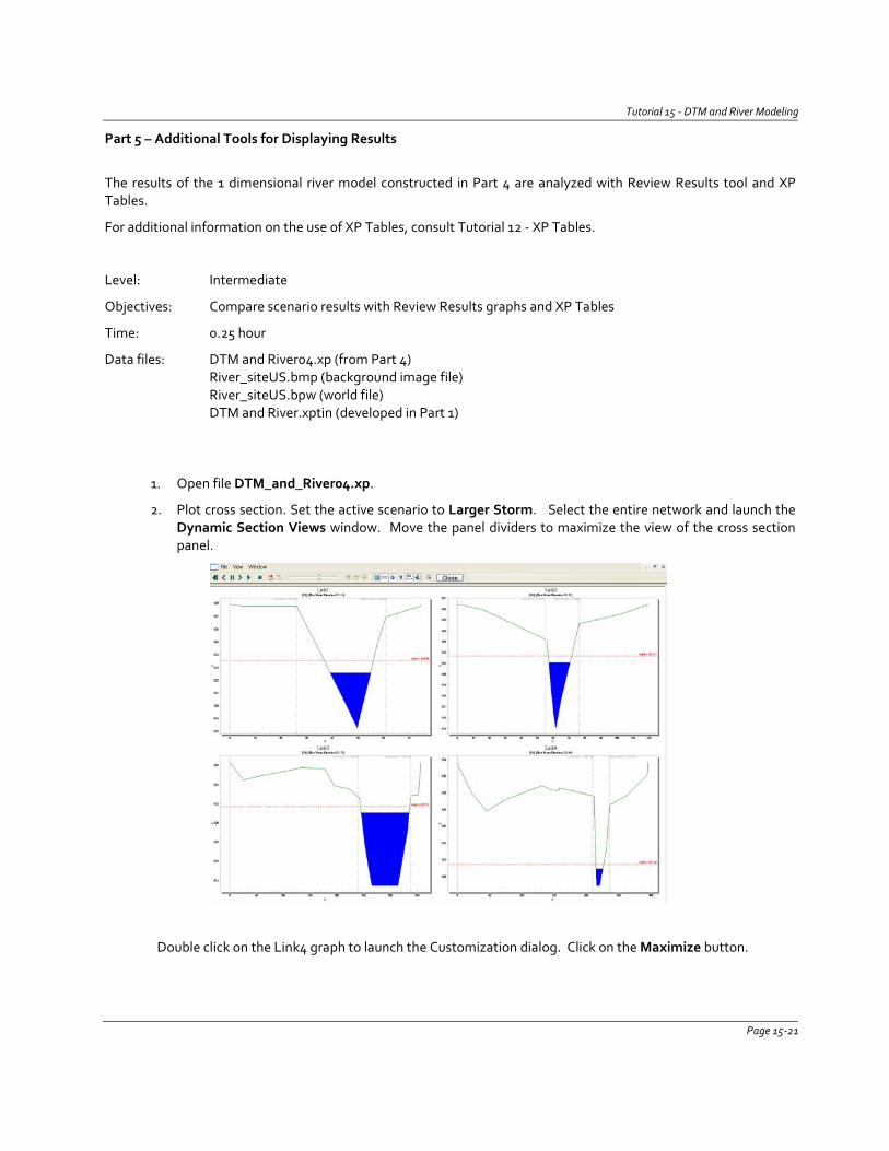
Tutorial 15 - DTM and River Modeling
Part 5 – Additional Tools for Displaying Results
The results of the 1 dimensional river model constructed in Part 4 are analyzed with Review Results tool and XP Tables.
For additional information on the use of XP Tables, consult Tutorial 12 - XP Tables.
Level: Intermediate
Objectives: Compare scenario results with Review Results graphs and XP Tables
Time: 0.25 hour
Data files: DTM and River04.xp (from Part 4) River_siteUS.bmp (background image file)
River_siteUS.bpw (world file) DTM and River.xptin (developed in Part 1)
1. Open file DTM_and_River04.xp.
2. Plot cross section. Set the active scenario to Larger Storm. Select the entire network and launch the Dynamic Section Views window. Move the panel dividers to maximize the view of the cross section panel.
Double click on the Link4 graph to launch the Customization dialog. Click on the Maximize button.
Page 15-21
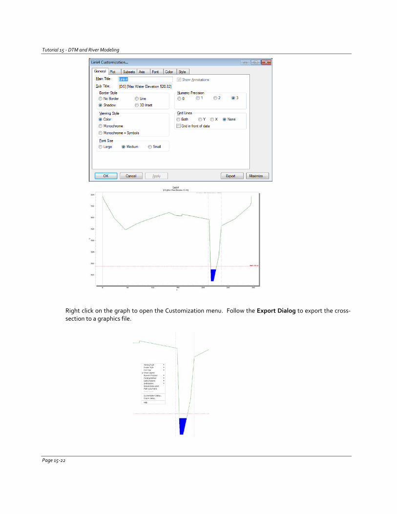
Tutorial 15 - DTM and River Modeling
Right click on the graph to open the Customization menu. Follow the Export Dialog to export the cross-section to a graphics file.
Page 15-22
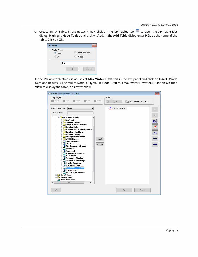
Tutorial 15 - DTM and River Modeling
3. Create an XP Table. In the network view click on the XP Tables tool to open the XP Table List dialog. Highlight Node Tables and click on Add. In the Add Table dialog enter HGL as the name of the table. Click on OK.
In the Variable Selection dialog, select Max Water Elevation in the left panel and click on Insert. (Node Data and Results -> Hydraulics Node -> Hydraulic Node Results ->Max Water Elevation). Click on OK then View to display the table in a new window.
Page 15-23
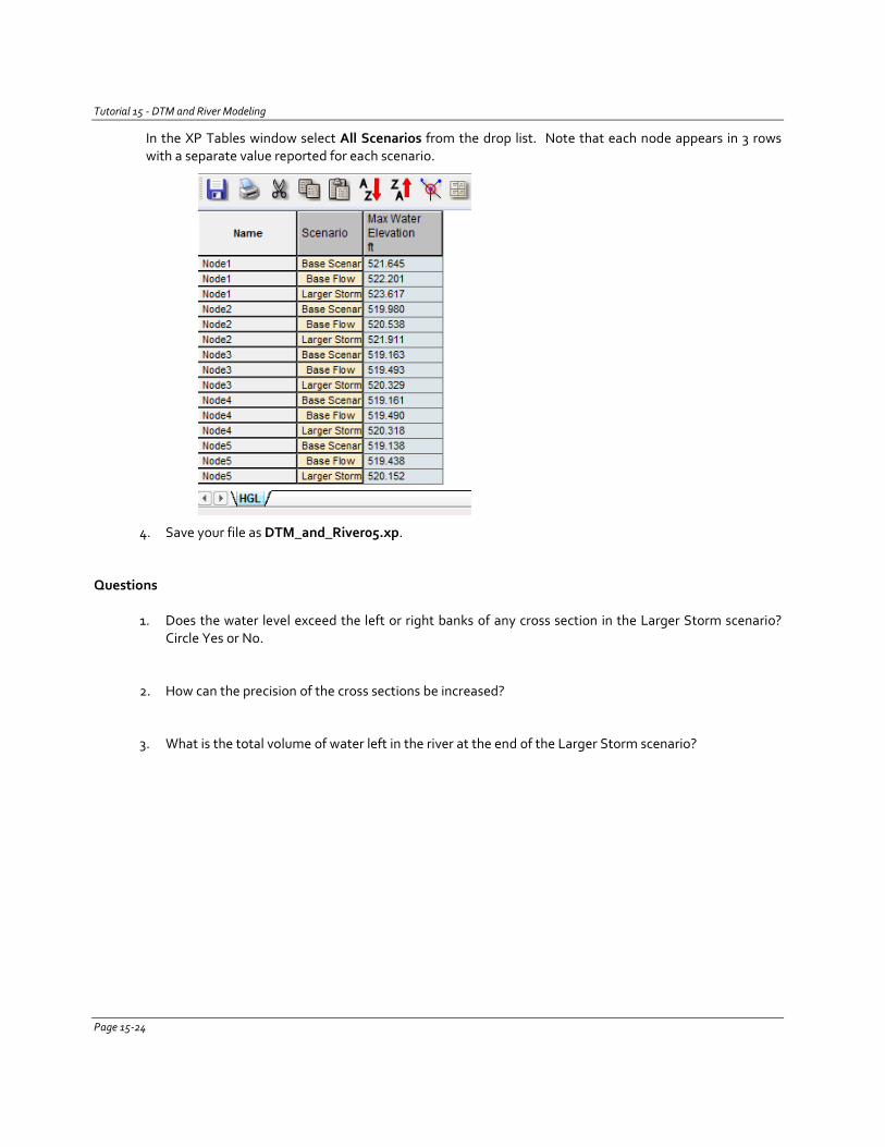
Tutorial 15 - DTM and River Modeling
In the XP Tables window select All Scenarios from the drop list. Note that each node appears in 3 rows with a separate value reported for each scenario.
4. Save your file as DTM_and_River05.xp.
Questions
1. Does the water level exceed the left or right banks of any cross section in the Larger Storm scenario? Circle Yes or No.
2. How can the precision of the cross sections be increased?
3. What is the total volume of water left in the river at the end of the Larger Storm scenario?
Page 15-24
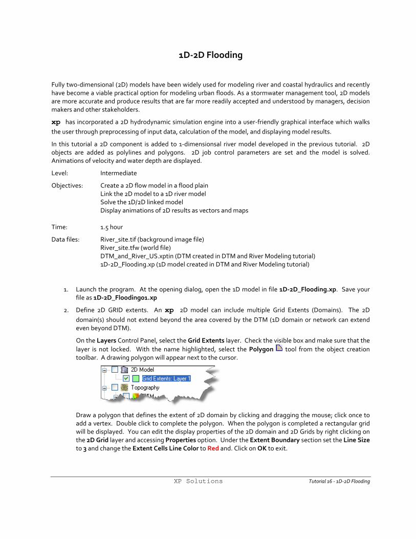
1D-2D Flooding
Fully two-dimensional (2D) models have been widely used for modeling river and coastal hydraulics and recently have become a viable practical option for modeling urban floods. As a stormwater management tool, 2D models are more accurate and produce results that are far more readily accepted and understood by managers, decision makers and other stakeholders.
xp has incorporated a 2D hydrodynamic simulation engine into a user-friendly graphical interface which walks the user through preprocessing of input data, calculation of the model, and displaying model results.
In this tutorial a 2D component is added to 1-dimensionsal river model developed in the previous tutorial. 2D objects are added as polylines and polygons. 2D job control parameters are set and the model is solved. Animations of velocity and water depth are displayed.
Level: Intermediate
Objectives: Create a 2D flow model in a flood plain Link the 2D model to a 1D river model Solve the 1D/2D linked model Display animations of 2D results as vectors and maps Time: 1.5 hour
Data files: River_site.tif (background image file) River_site.tfw (world file) DTM_and_River_US.xptin (DTM created in DTM and River Modeling tutorial) 1D-2D_Flooding.xp (1D model created in DTM and River Modeling tutorial)
1. Launch the program. At the opening dialog, open the 1D model in file 1D-2D_Flooding.xp. Save your file as 1D-2D_Flooding01.xp
2. Define 2D GRID extents. An xp 2D model can include multiple Grid Extents (Domains). The 2D domain(s) should not extend beyond the area covered by the DTM (1D domain or network can extend even beyond DTM).
On the Layers Control Panel, select the Grid Extents layer. Check the visible box and make sure that the layer is not locked. With the name highlighted, select the Polygon tool from the object creation toolbar. A drawing polygon will appear next to the cursor.
Draw a polygon that defines the extent of 2D domain by clicking and dragging the mouse; click once to add a vertex. Double click to complete the polygon. When the polygon is completed a rectangular grid will be displayed. You can edit the display properties of the 2D domain and 2D Grids by right clicking on the 2D Grid layer and accessing Properties option. Under the Extent Boundary section set the Line Size to 3 and change the Extent Cells Line Color to Red and. Click on OK to exit.
XP Solutions Tutorial 16 - 1D-2D Flooding
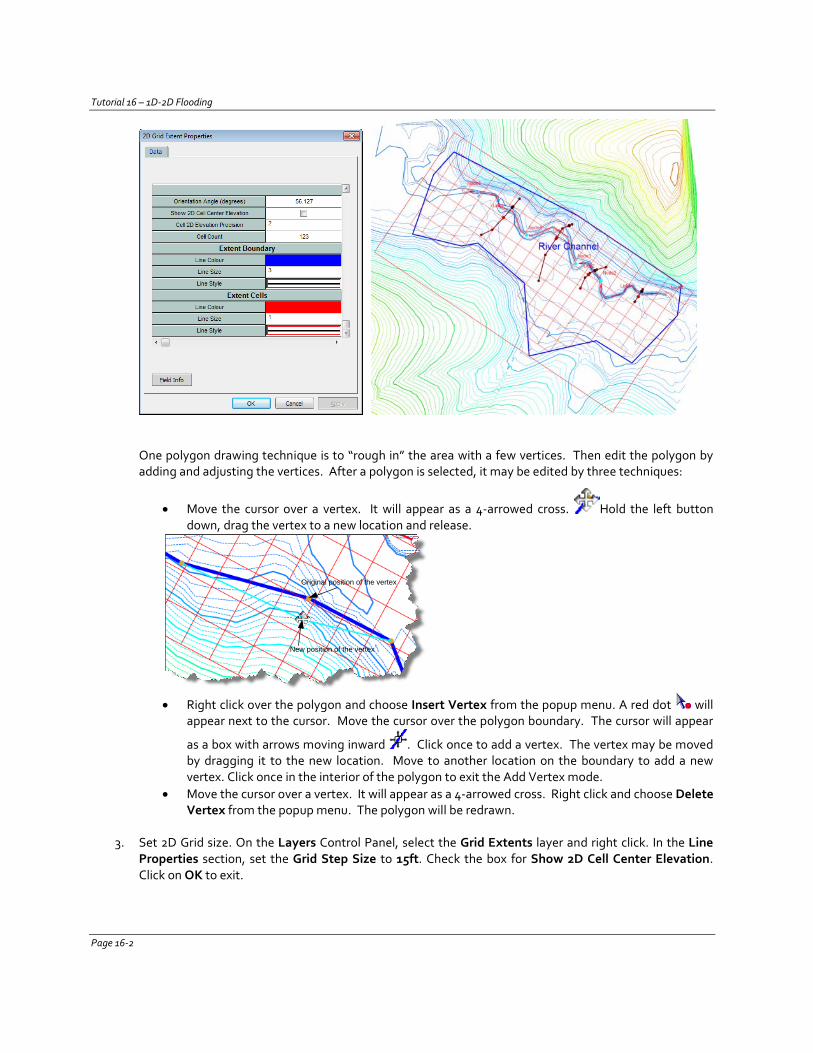
Tutorial 16 – 1D-2D Flooding
One polygon drawing technique is to “rough in” the area with a few vertices. Then edit the polygon by adding and adjusting the vertices. After a polygon is selected, it may be edited by three techniques:
• Move the cursor over a vertex. It will appear as a 4-arrowed cross. Hold the left button down, drag the vertex to a new location and release.
Original position of the vertex
New position of the vertex
• Right click over the polygon and choose Insert Vertex from the popup menu. A red dot will
appear next to the cursor. Move the cursor over the polygon boundary. The cursor will appear
as a box with arrows moving inward . Click once to add a vertex. The vertex may be moved by dragging it to the new location. Move to another location on the boundary to add a new vertex. Click once in the interior of the polygon to exit the Add Vertex mode.
• Move the cursor over a vertex. It will appear as a 4-arrowed cross. Right click and choose Delete Vertex from the popup menu. The polygon will be redrawn.
3. Set 2D Grid size. On the Layers Control Panel, select the Grid Extents layer and right click. In the Line
Properties section, set the Grid Step Size to 15ft. Check the box for Show 2D Cell Center Elevation. Click on OK to exit.
Page 16-2
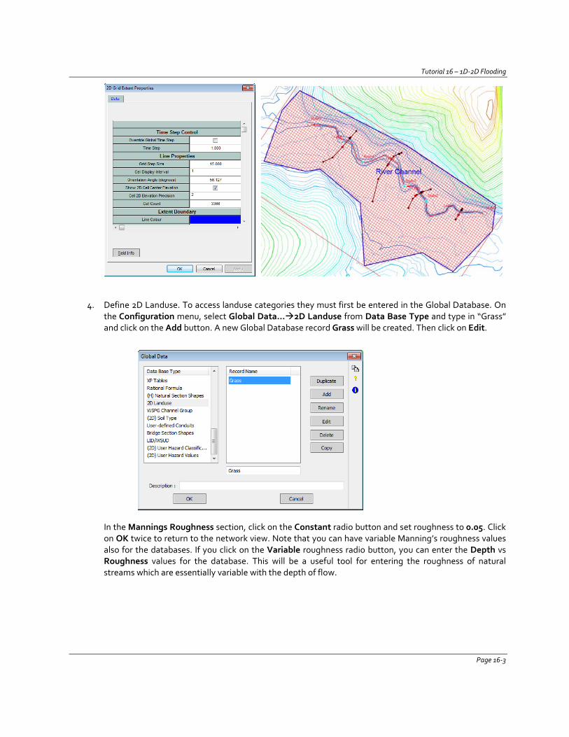
Tutorial 16 – 1D-2D Flooding
4. Define 2D Landuse. To access landuse categories they must first be entered in the Global Database. On
the Configuration menu, select Global Data…2D Landuse from Data Base Type and type in “Grass” and click on the Add button. A new Global Database record Grass will be created. Then click on Edit.
In the Mannings Roughness section, click on the Constant radio button and set roughness to 0.05. Click on OK twice to return to the network view. Note that you can have variable Manning’s roughness values also for the databases. If you click on the Variable roughness radio button, you can enter the Depth vs Roughness values for the database. This will be a useful tool for entering the roughness of natural streams which are essentially variable with the depth of flow.
Page 16-3
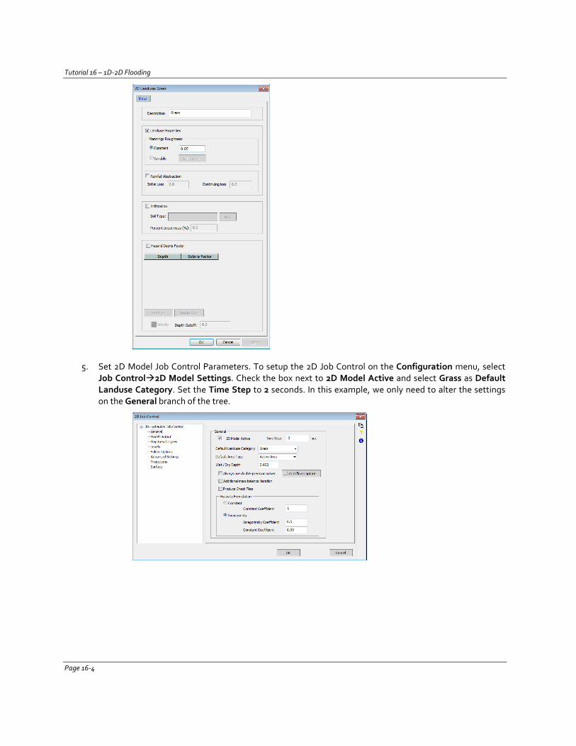
Tutorial 16 – 1D-2D Flooding
5. Set 2D Model Job Control Parameters. To setup the 2D Job Control on the Configuration menu, select Job Control2D Model Settings. Check the box next to 2D Model Active and select Grass as Default Landuse Category. Set the Time Step to 2 seconds. In this example, we only need to alter the settings on the General branch of the tree.
Page 16-4
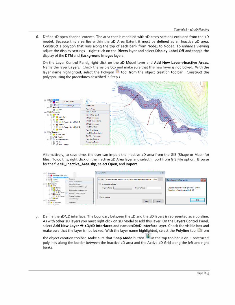
Tutorial 16 – 1D-2D Flooding
6. Define 1D open channel extents. The area that is modeled with 1D cross-sections excluded from the 2D model. Because this area lies within the 2D Area Extent it must be defined as an Inactive 2D area. Construct a polygon that runs along the top of each bank from Node1 to Node5. To enhance viewing adjust the display settings – right-click on the Rivers layer and select Display Label Off and toggle the display of the DTM and Background Images layers.
On the Layer Control Panel, right-click on the 2D Model layer and Add New Layer->Inactive Areas. Name the layer Layer1. Check the visible box and make sure that this new layer is not locked. With the layer name highlighted, select the Polygon tool from the object creation toolbar. Construct the polygon using the procedures described in Step 2.
Alternatively, to save time, the user can import the inactive 2D area from the GIS (Shape or Mapinfo) files. To do this, right click on the Inactive 2D Area layer and select Import from GIS File option. Browse for the file 2D_Inactive_Area.shp, select Open, and Import.
7. Define the 1D/2D interface. The boundary between the 1D and the 2D layers is represented as a polyline. As with other 2D layers you must right click on 2D Model to add this layer. On the Layers Control Panel, select Add New Layer 1D/2D Interfaces and named1D/2D Interface layer. Check the visible box and make sure that the layer is not locked. With the layer name highlighted, select the Polyline tool from
the object creation toolbar. Make sure that Snap Mode button in the top toolbar is on. Construct 2 polylines along the border between the Inactive 2D area and the Active 2D Grid along the left and right banks.
Page 16-5
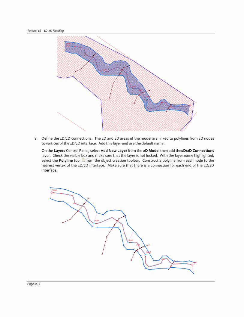
Tutorial 16 – 1D-2D Flooding
8. Define the 1D/2D connections. The 1D and 2D areas of the model are linked to polylines from 1D nodes to vertices of the 1D/2D interface. Add this layer and use the default name.
On the Layers Control Panel, select Add New Layer from the 2D Model then add the1D/2D Connections layer. Check the visible box and make sure that the layer is not locked. With the layer name highlighted, select the Polyline tool from the object creation toolbar. Construct a polyline from each node to the nearest vertex of the 1D/2D interface. Make sure that there is a connection for each end of the 1D/2D interface.
Page 16-6
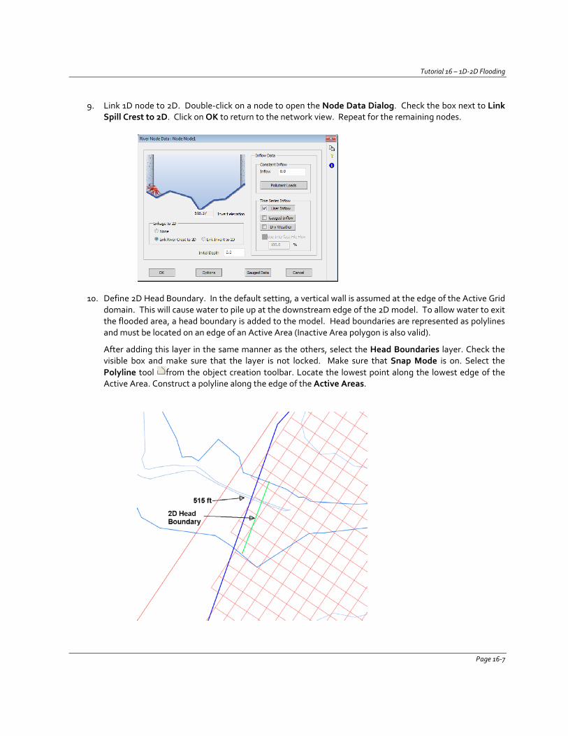
Tutorial 16 – 1D-2D Flooding
9. Link 1D node to 2D. Double-click on a node to open the Node Data Dialog. Check the box next to Link Spill Crest to 2D. Click on OK to return to the network view. Repeat for the remaining nodes.
10. Define 2D Head Boundary. In the default setting, a vertical wall is assumed at the edge of the Active Grid
domain. This will cause water to pile up at the downstream edge of the 2D model. To allow water to exit the flooded area, a head boundary is added to the model. Head boundaries are represented as polylines and must be located on an edge of an Active Area (Inactive Area polygon is also valid).
After adding this layer in the same manner as the others, select the Head Boundaries layer. Check the visible box and make sure that the layer is not locked. Make sure that Snap Mode is on. Select the Polyline tool from the object creation toolbar. Locate the lowest point along the lowest edge of the Active Area. Construct a polyline along the edge of the Active Areas.
Page 16-7
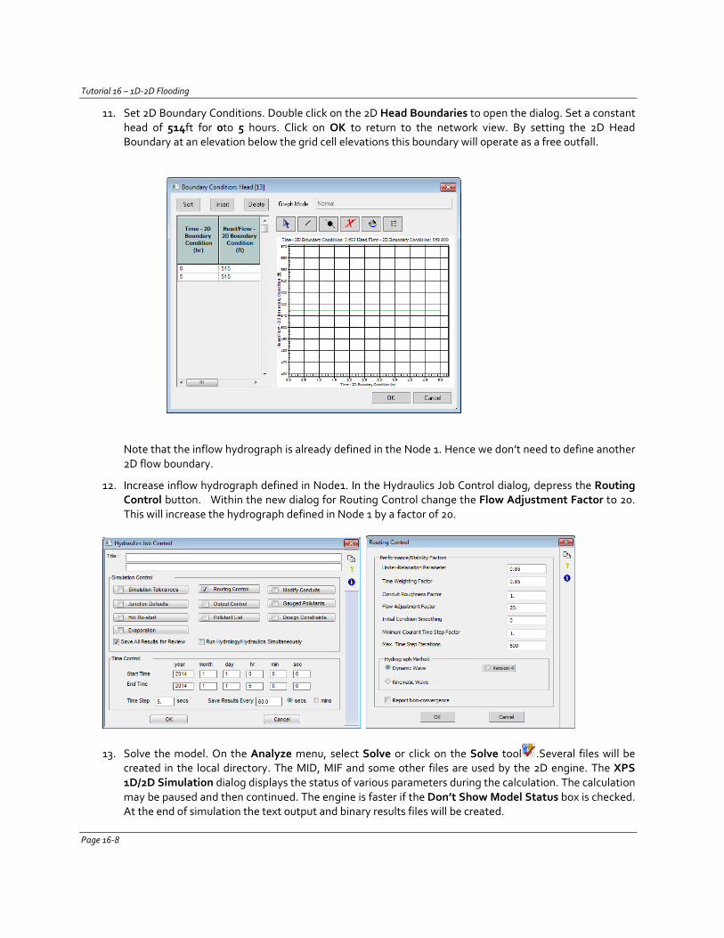
Tutorial 16 – 1D-2D Flooding
11. Set 2D Boundary Conditions. Double click on the 2D Head Boundaries to open the dialog. Set a constant head of 514ft for 0to 5 hours. Click on OK to return to the network view. By setting the 2D Head Boundary at an elevation below the grid cell elevations this boundary will operate as a free outfall.
Note that the inflow hydrograph is already defined in the Node 1. Hence we don’t need to define another 2D flow boundary.
12. Increase inflow hydrograph defined in Node1. In the Hydraulics Job Control dialog, depress the Routing Control button. Within the new dialog for Routing Control change the Flow Adjustment Factor to 20. This will increase the hydrograph defined in Node 1 by a factor of 20.
13. Solve the model. On the Analyze menu, select Solve or click on the Solve tool .Several files will be created in the local directory. The MID, MIF and some other files are used by the 2D engine. The XPS 1D/2D Simulation dialog displays the status of various parameters during the calculation. The calculation may be paused and then continued. The engine is faster if the Don’t Show Model Status box is checked. At the end of simulation the text output and binary results files will be created.
Page 16-8
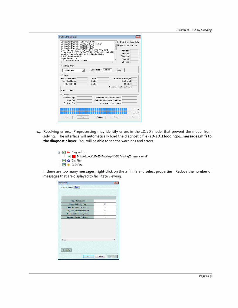
Tutorial 16 – 1D-2D Flooding
14. Resolving errors. Preprocessing may identify errors in the 1D/2D model that prevent the model from
solving. The interface will automatically load the diagnostic file (1D-2D_Flooding01_messages.mif) to the diagnostic layer. You will be able to see the warnings and errors.
If there are too many messages, right-click on the .mif file and select properties. Reduce the number of messages that are displayed to facilitate viewing.
Page 16-9
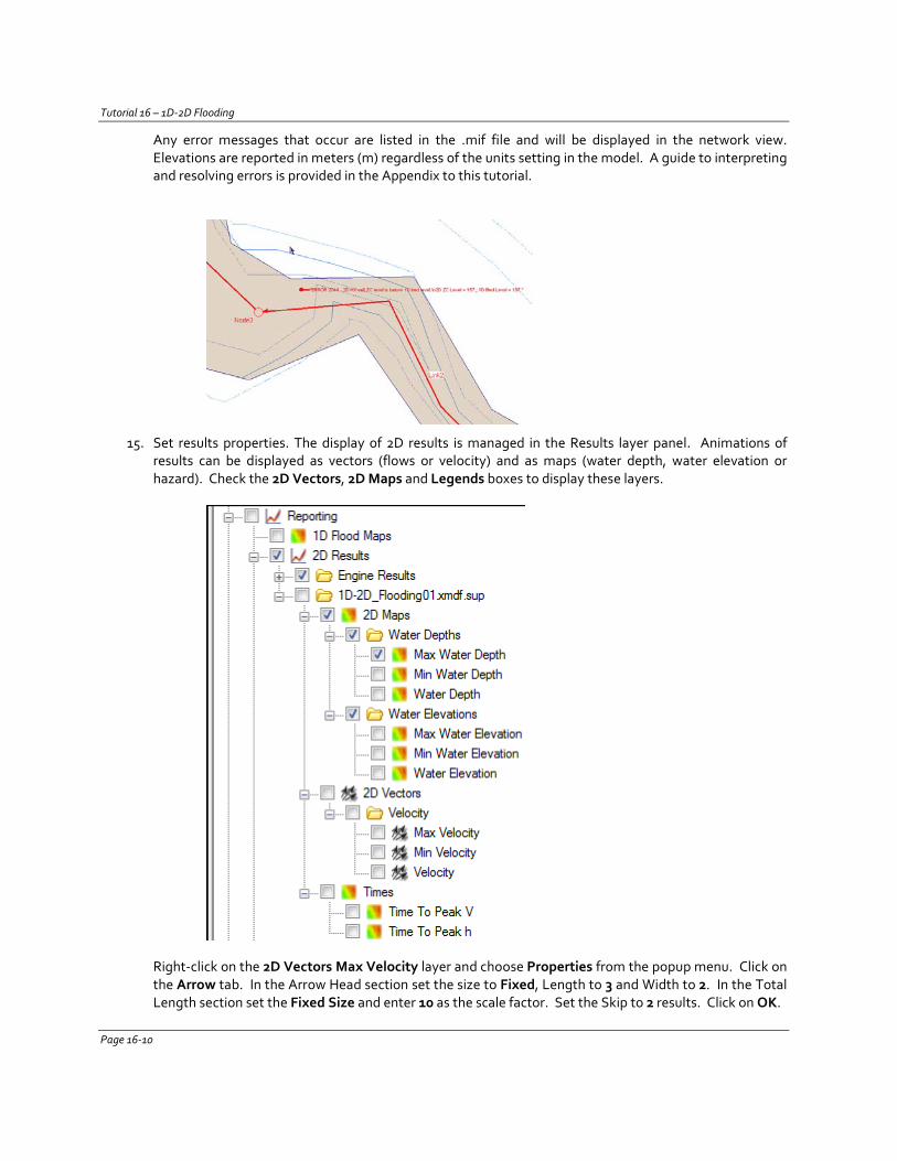
Tutorial 16 – 1D-2D Flooding
Any error messages that occur are listed in the .mif file and will be displayed in the network view. Elevations are reported in meters (m) regardless of the units setting in the model. A guide to interpreting and resolving errors is provided in the Appendix to this tutorial.
15. Set results properties. The display of 2D results is managed in the Results layer panel. Animations of results can be displayed as vectors (flows or velocity) and as maps (water depth, water elevation or hazard). Check the 2D Vectors, 2D Maps and Legends boxes to display these layers.
Right-click on the 2D Vectors Max Velocity layer and choose Properties from the popup menu. Click on the Arrow tab. In the Arrow Head section set the size to Fixed, Length to 3 and Width to 2. In the Total Length section set the Fixed Size and enter 10 as the scale factor. Set the Skip to 2 results. Click on OK.
Page 16-10
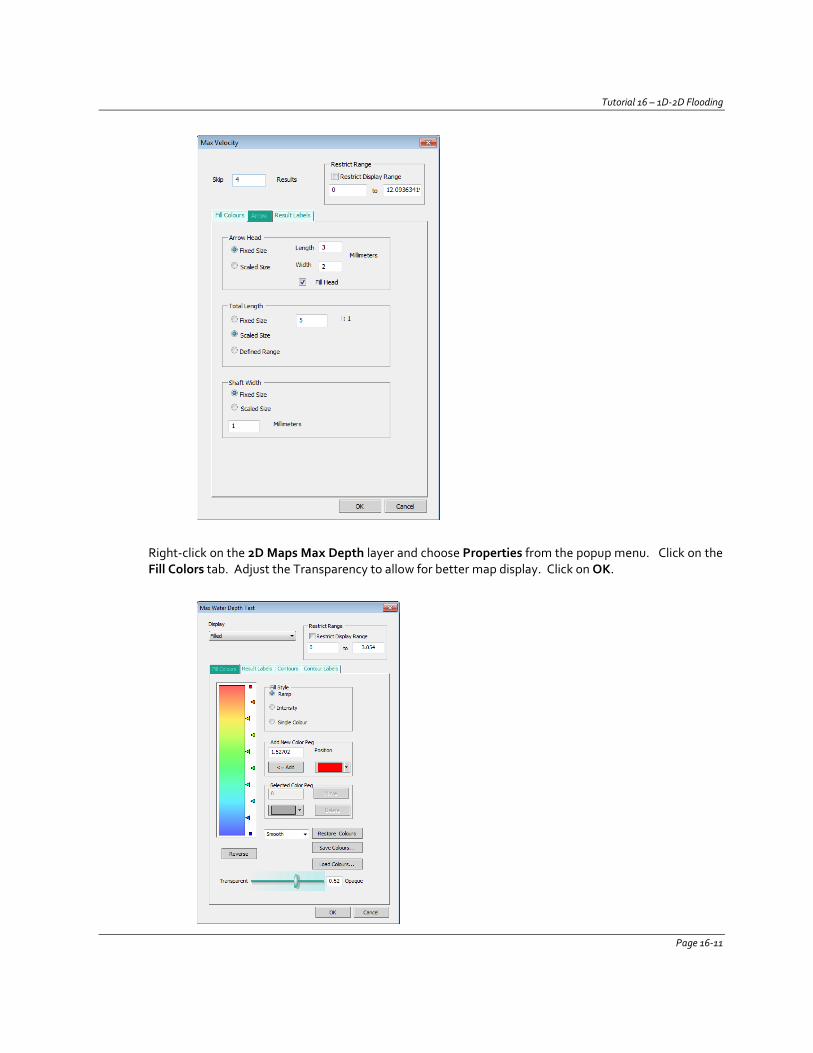
Tutorial 16 – 1D-2D Flooding
Right-click on the 2D Maps Max Depth layer and choose Properties from the popup menu. Click on the Fill Colors tab. Adjust the Transparency to allow for better map display. Click on OK.
Page 16-11
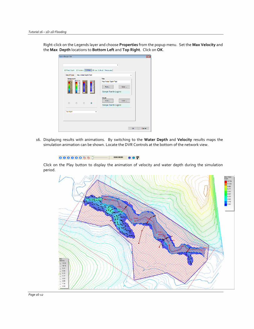
Tutorial 16 – 1D-2D Flooding
Right-click on the Legends layer and choose Properties from the popup menu. Set the Max Velocity and the Max Depth locations to Bottom Left and Top Right. Click on OK.
16. Displaying results with animations. By switching to the Water Depth and Velocity results maps the
simulation animation can be shown. Locate the DVR Controls at the bottom of the network view.
Click on the Play button to display the animation of velocity and water depth during the simulation period.
Page 16-12

Tutorial 16 – 1D-2D Flooding
Questions
1. At what time does the stream flow over its banks?
2. What is the maximum width of the flooded area between Node1 and Node5?
3. Does the floodplain drain by the end of the simulation?
Page 16-13
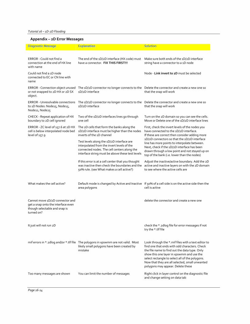
Tutorial 16 – 1D-2D Flooding
Appendix – 2D Error Messages
Diagnostic Message Explanation Solution
ERROR - Could not find a connection at the end of HX line with name
The end of the 1D/2D interface (HX code) must have a connector. FIX THIS FIRST!!!
Make sure both ends of the 1D/2D interface string have a connector to a 1D node
Could not find a 1D node connected to EC or CN line with name
Node - Link invert to 2D must be selected
ERROR - Connection object unused or not snapped to 2D HX or 2D SX object.
The 1D/2D connector no longer connects to the 1D/2D interface
Delete the connector and create a new one so that the snap will work
ERROR - Unresolvable connections to 1D Nodes: Node15, Node15, Node11, Node25
The 1D/2D connector no longer connects to the 1D/2D interface
Delete the connector and create a new one so that the snap will work
CHECK - Repeat application of HX boundary to 2D cell ignored
Two of the 1D/2D interfaces lines go through one cell
Turn on the 2D domain so you can see the cells. Move or Delete one of the 1D/2D interface lines
ERROR - ZC level of 157.6 at 2D HX cell is below interpolated node bed level of 157.9
The 2D cells that form the banks along the 1D/2D interface must be higher than the nodes inverts of the 1D channel
Test levels along the 1D/2D interface are interpolated from the invert levels of the connected nodes. The cell centers along the interface string must be above these test levels
First, check the invert levels of the nodes you have connected to the 1D/2D interface. If these are correct then consider adding more 1D/2D connectors so that the 1D/2D interface line has more points to interpolate between. Next, check if the 1D/2D interface has been drawn through a low point and not stayed up on top of the bank (i.e. lower than the nodes)
If this error is at a cell center that you thought was inactive then check the boundaries and the 50% rule. (see What makes a cell active?)
Adjust the inactive/active boundary. Add the 2D active and inactive layers on with the 2D domain to see where the active cells are
What makes the cell active? Default mode is changed by Active and Inactive area polygons
If 50% of a cell side is on the active side then the cell is active
Cannot move 1D/2D connector and get a snap onto the interface even though selectable and snap is turned on?
delete the connector and create a new one
It just will not run 2D check the *.2dlog file for error messages if not try the *.tlf file
mif errors in *.2dlog and/or *.tlf file The polygons in xpswmm are not valid. Most likely small polygons have been created by mistake
Look through the *.mif files with a text editor to find one that ends with odd characters. Check the file name to find out the data type. Only show this one layer in xpswmm and use the select rectangle to select all of the polygons. Now that they are all selected, small unwanted polygons may appear. Delete these
Too many messages are shown You can limit the number of messages Right click in layer control on the diagnostic file and change setting on data tab
Page 16-14
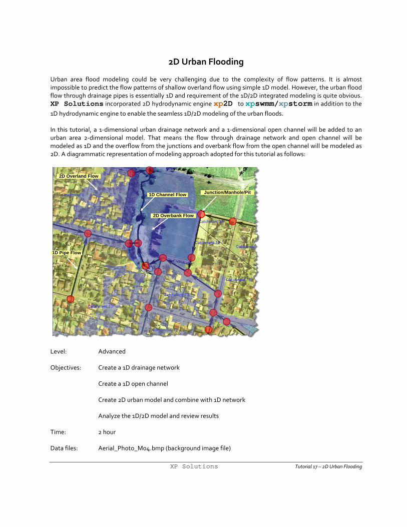
2D Urban Flooding
Urban area flood modeling could be very challenging due to the complexity of flow patterns. It is almost impossible to predict the flow patterns of shallow overland flow using simple 1D model. However, the urban flood flow through drainage pipes is essentially 1D and requirement of the 1D/2D integrated modeling is quite obvious. XP Solutions incorporated 2D hydrodynamic engine xp2D to xpswmm/xpstorm in addition to the 1D hydrodynamic engine to enable the seamless 1D/2D modeling of the urban floods.
In this tutorial, a 1-dimensional urban drainage network and a 1-dimensional open channel will be added to an urban area 2-dimensional model. That means the flow through drainage network and open channel will be modeled as 1D and the overflow from the junctions and overbank flow from the open channel will be modeled as 2D. A diagrammatic representation of modeling approach adopted for this tutorial as follows:
Junction/Manhole/Pit
1D Pipe Flow
2D Overland Flow
1D Channel Flow
2D Overbank Flow
Level: Advanced
Objectives: Create a 1D drainage network
Create a 1D open channel
Create 2D urban model and combine with 1D network
Analyze the 1D/2D model and review results
Time: 2 hour
Data files: Aerial_Photo_M04.bmp (background image file)
XP Solutions Tutorial 17 – 2D Urban Flooding

Tutorial 17 – 2D Urban Flooding
Aerial_Photo_M04.bpw (world file)
Post_Development.xptin
Urban_Flooding01.xp (starter model which contains the global databases for design rainfall, loss model, and 2D Landuses); Urban_Flooding_Completed.xp (completed model file); Urban_Flooding_Completed_Pond.xp (completed model with a detention pond as mitigation).
!NOTE: The following section 1D Drainage Network and Hydrology, and 2D Model Setup are optional. This section describes the setting up of 1D drainage network and hydrology model. User may skip this section and go to the last section Analysis and Review Results. In that case, user can open the completed model Urban_Flooding_Completed.xp, analyze, and review results.
1D Drainage Network and Hydrology:
This section will describe how to set up a 1D drainage network model for the urban development. Note that this network is already designed and we will construct/import this designed network into our model.
1. Launch the program. At the opening dialogopen the Urban_Flooding01.xp. Save the model as Urban_Flooding02.xp.
2. Load background image. Right click on the Background Image layer and select the option Add Background Image. Browse for the file Aerial_Photo_M04.bmp, select and open the file. You will see an urban residential subdivision development, roadways, narrow open channels, playground, and ponds in the aerial map.
Page 17-2
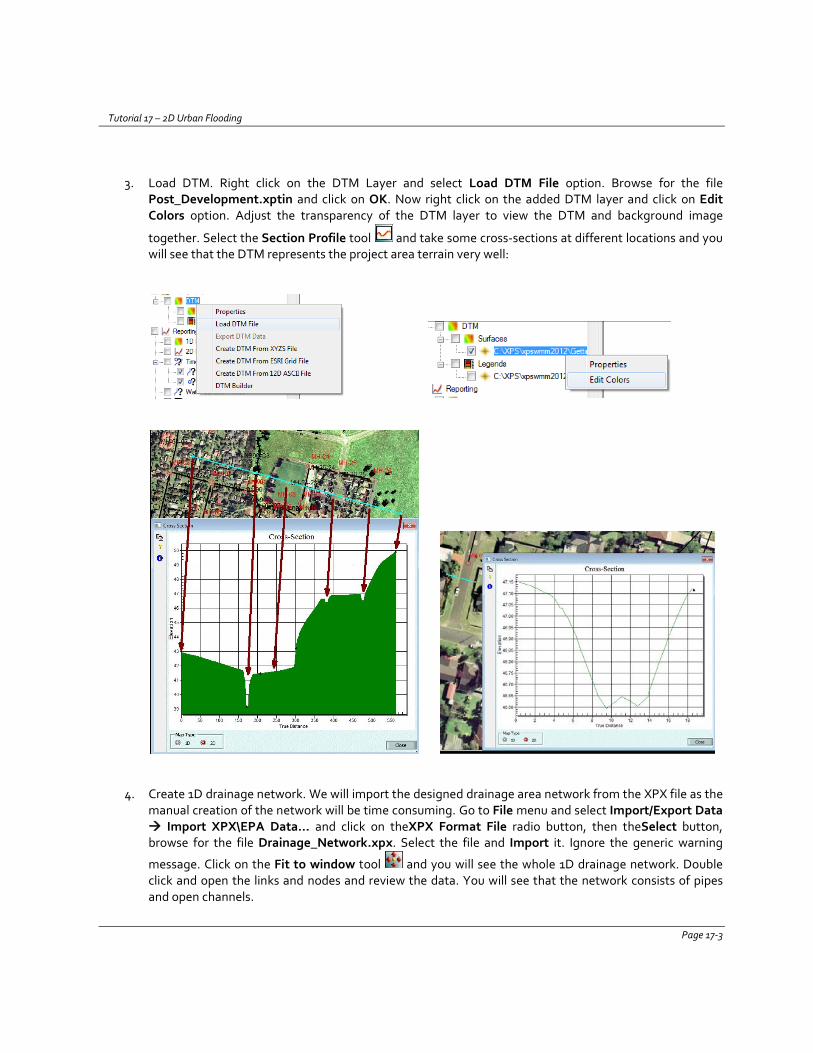
Tutorial 17 – 2D Urban Flooding
3. Load DTM. Right click on the DTM Layer and select Load DTM File option. Browse for the file Post_Development.xptin and click on OK. Now right click on the added DTM layer and click on Edit Colors option. Adjust the transparency of the DTM layer to view the DTM and background image
together. Select the Section Profile tool and take some cross-sections at different locations and you will see that the DTM represents the project area terrain very well:
4. Create 1D drainage network. We will import the designed drainage area network from the XPX file as the manual creation of the network will be time consuming. Go to File menu and select Import/Export Data Import XPX\EPA Data… and click on theXPX Format File radio button, then theSelect button, browse for the file Drainage_Network.xpx. Select the file and Import it. Ignore the generic warning
message. Click on the Fit to window tool and you will see the whole 1D drainage network. Double click and open the links and nodes and review the data. You will see that the network consists of pipes and open channels.
Page 17-3
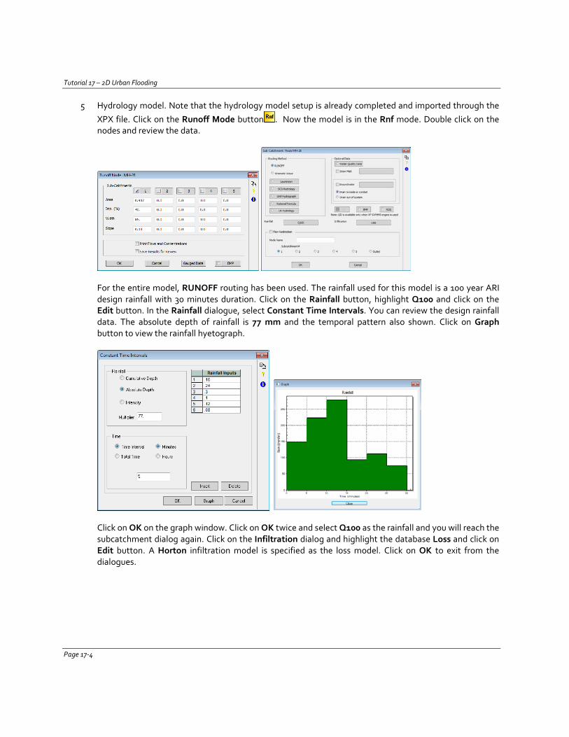
Tutorial 17 – 2D Urban Flooding
5 Hydrology model. Note that the hydrology model setup is already completed and imported through the XPX file. Click on the Runoff Mode button . Now the model is in the Rnf mode. Double click on the nodes and review the data.
For the entire model, RUNOFF routing has been used. The rainfall used for this model is a 100 year ARI design rainfall with 30 minutes duration. Click on the Rainfall button, highlight Q100 and click on the Edit button. In the Rainfall dialogue, select Constant Time Intervals. You can review the design rainfall data. The absolute depth of rainfall is 77 mm and the temporal pattern also shown. Click on Graph button to view the rainfall hyetograph.
Click on OK on the graph window. Click on OK twice and select Q100 as the rainfall and you will reach the subcatchment dialog again. Click on the Infiltration dialog and highlight the database Loss and click on Edit button. A Horton infiltration model is specified as the loss model. Click on OK to exit from the dialogues.
Page 17-4
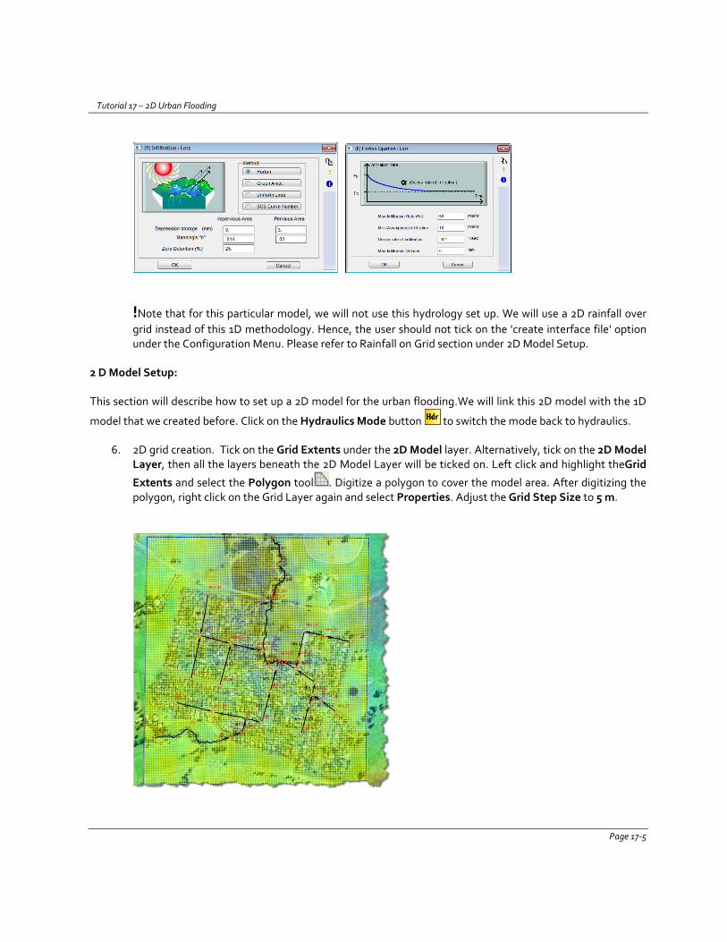
Tutorial 17 – 2D Urban Flooding
!Note that for this particular model, we will not use this hydrology set up. We will use a 2D rainfall over grid instead of this 1D methodology. Hence, the user should not tick on the 'create interface file' option under the Configuration Menu. Please refer to Rainfall on Grid section under 2D Model Setup.
2 D Model Setup:
This section will describe how to set up a 2D model for the urban flooding.We will link this 2D model with the 1D
model that we created before. Click on the Hydraulics Mode button to switch the mode back to hydraulics.
6. 2D grid creation. Tick on the Grid Extents under the 2D Model layer. Alternatively, tick on the 2D Model Layer, then all the layers beneath the 2D Model Layer will be ticked on. Left click and highlight theGrid
Extents and select the Polygon tool . Digitize a polygon to cover the model area. After digitizing the polygon, right click on the Grid Layer again and select Properties. Adjust the Grid Step Size to 5 m.
Page 17-5
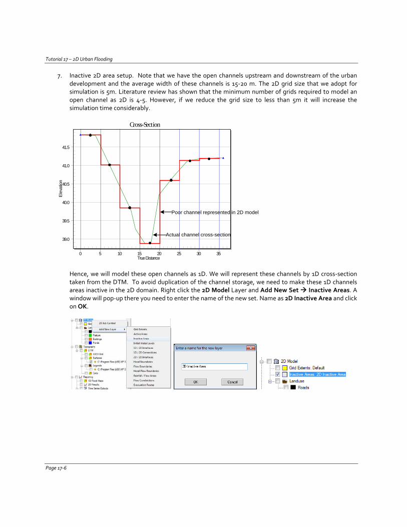
Tutorial 17 – 2D Urban Flooding
7. Inactive 2D area setup. Note that we have the open channels upstream and downstream of the urban development and the average width of these channels is 15-20 m. The 2D grid size that we adopt for simulation is 5m. Literature review has shown that the minimum number of grids required to model an open channel as 2D is 4-5. However, if we reduce the grid size to less than 5m it will increase the simulation time considerably.
39.0
39.5
40.0
40.5
41.0
41.5
0 5 10 15 20 25 30 35
Cross-Section
Elev
atio
n
True Distance
Actual channel cross-section
Poor channel represented in 2D model
Hence, we will model these open channels as 1D. We will represent these channels by 1D cross-section taken from the DTM. To avoid duplication of the channel storage, we need to make these 1D channels areas inactive in the 2D domain. Right click the 2D Model Layer and Add New Set Inactive Areas. A window will pop-up there you need to enter the name of the new set. Name as 2D Inactive Area and click on OK.
Page 17-6
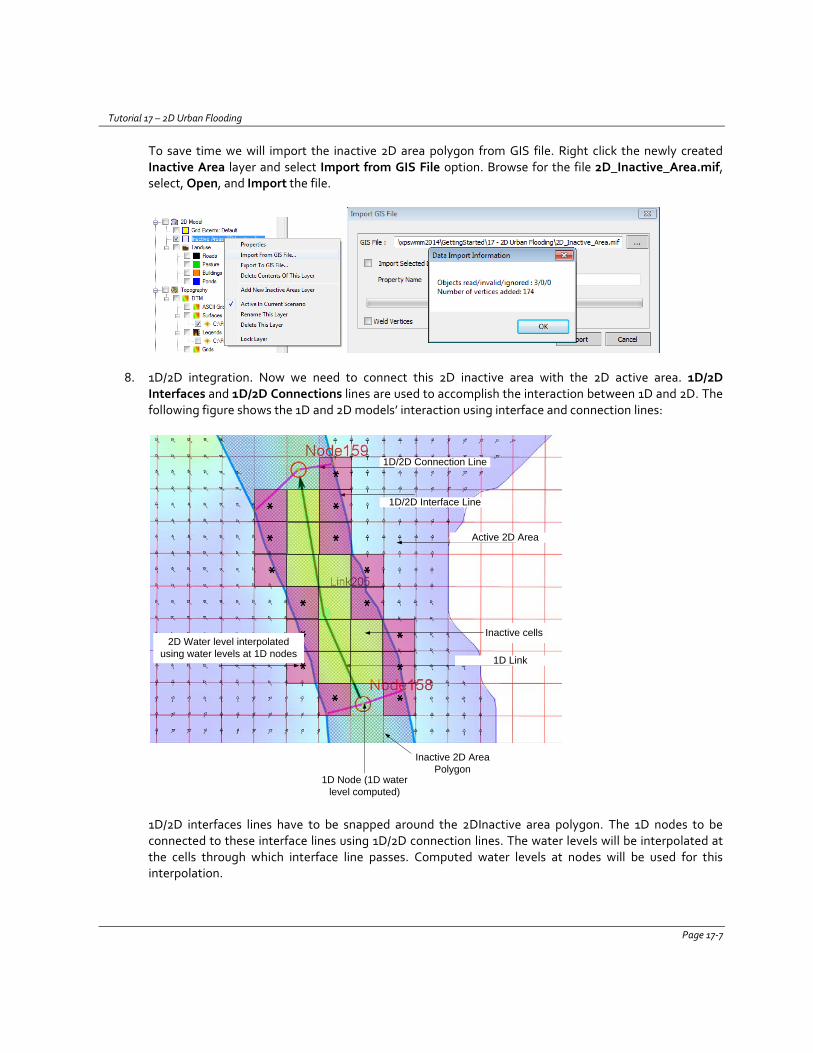
Tutorial 17 – 2D Urban Flooding
To save time we will import the inactive 2D area polygon from GIS file. Right click the newly created Inactive Area layer and select Import from GIS File option. Browse for the file 2D_Inactive_Area.mif, select, Open, and Import the file.
8. 1D/2D integration. Now we need to connect this 2D inactive area with the 2D active area. 1D/2D Interfaces and 1D/2D Connections lines are used to accomplish the interaction between 1D and 2D. The following figure shows the 1D and 2D models’ interaction using interface and connection lines:
1D Node (1D water level computed)
1D Link
Inactive 2D Area Polygon
Active 2D Area
1D/2D Interface Line
1D/2D Connection Line
2D Water level interpolated using water levels at 1D nodes
Inactive cells
1D/2D interfaces lines have to be snapped around the 2DInactive area polygon. The 1D nodes to be connected to these interface lines using 1D/2D connection lines. The water levels will be interpolated at the cells through which interface line passes. Computed water levels at nodes will be used for this interpolation.
Page 17-7
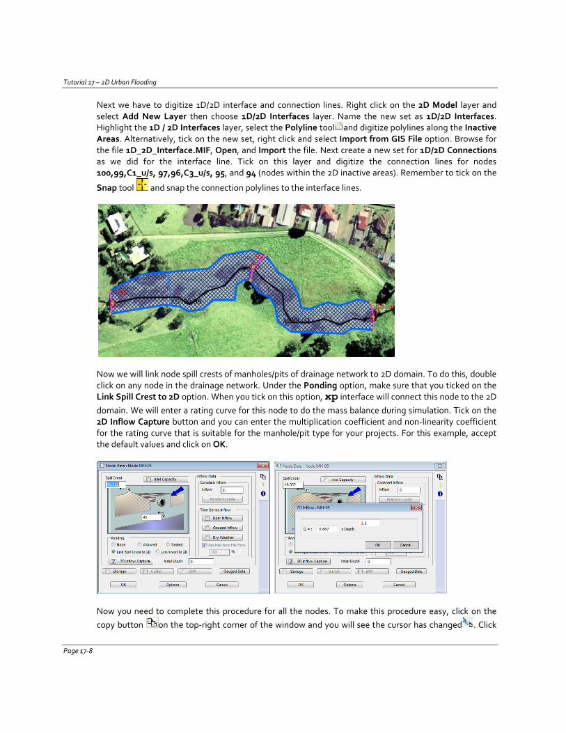
Tutorial 17 – 2D Urban Flooding
Next we have to digitize 1D/2D interface and connection lines. Right click on the 2D Model layer and select Add New Layer then choose 1D/2D Interfaces layer. Name the new set as 1D/2D Interfaces. Highlight the 1D / 2D Interfaces layer, select the Polyline tool and digitize polylines along the Inactive Areas. Alternatively, tick on the new set, right click and select Import from GIS File option. Browse for the file 1D_2D_Interface.MIF, Open, and Import the file. Next create a new set for 1D/2D Connections as we did for the interface line. Tick on this layer and digitize the connection lines for nodes 100,99,C1_u/s, 97,96,C3_u/s, 95, and 94 (nodes within the 2D inactive areas). Remember to tick on the
Snap tool and snap the connection polylines to the interface lines.
Now we will link node spill crests of manholes/pits of drainage network to 2D domain. To do this, double click on any node in the drainage network. Under the Ponding option, make sure that you ticked on the Link Spill Crest to 2D option. When you tick on this option, xp interface will connect this node to the 2D domain. We will enter a rating curve for this node to do the mass balance during simulation. Tick on the 2D Inflow Capture button and you can enter the multiplication coefficient and non-linearity coefficient for the rating curve that is suitable for the manhole/pit type for your projects. For this example, accept the default values and click on OK.
Now you need to complete this procedure for all the nodes. To make this procedure easy, click on the copy button on the top-right corner of the window and you will see the cursor has changed . Click
Page 17-8
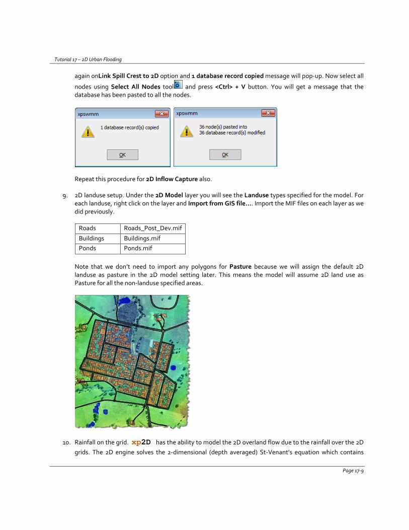
Tutorial 17 – 2D Urban Flooding
again onLink Spill Crest to 2D option and 1 database record copied message will pop-up. Now select all
nodes using Select All Nodes tool and press <Ctrl> + V button. You will get a message that the database has been pasted to all the nodes.
Repeat this procedure for 2D Inflow Capture also.
9. 2D landuse setup. Under the 2D Model layer you will see the Landuse types specified for the model. For each landuse, right click on the layer and Import from GIS file…. Import the MIF files on each layer as we did previously.
Roads Roads_Post_Dev.mif
Buildings Buildings.mif Ponds Ponds.mif
Note that we don’t need to import any polygons for Pasture because we will assign the default 2D landuse as pasture in the 2D model setting later. This means the model will assume 2D land use as Pasture for all the non-landuse specified areas.
10. Rainfall on the grid. xp2D has the ability to model the 2D overland flow due to the rainfall over the 2D grids. The 2D engine solves the 2-dimensional (depth averaged) St-Venant’s equation which contains
Page 17-9
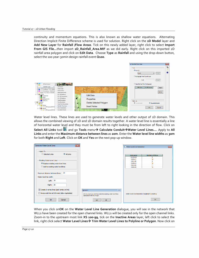
Tutorial 17 – 2D Urban Flooding
continuity and momentum equations. This is also known as shallow water equations. Alternating Direction Implicit Finite Difference scheme is used for solution. Right click on the 2D Model layer and Add New Layer for Rainfall /Flow Areas. Tick on this newly added layer, right click to select Import From GIS File…then import 2D_Rainfall_Area.MIF as we did early. Right click on this imported 2D rainfall area polygon and click on Edit Data. Choose Type as Rainfall and using the drop-down button, select the 100 year-30min design rainfall event Q100.
Water level lines. These lines are used to generate water levels and other output of 1D domain. This allows the combined viewing of 2D and 1D domain results together. A water level line is essentially a line of horizontal water level and they must be from left to right looking in the direction of flow. Click on Select All Links tool and go Tools menu Calculate ConduitWater Level Lines…. Apply to All Links and enter the Maximum distance between lines as 20m. Enter the Water level line widths as 30m for both Right and Left. Click on OK and Yes on the next pop-up window.
When you click onOK on the Water Level Line Generation dialogue, you will see in the network that WLLs have been created for the open channel links. WLLs will be created only for the open channel links. Zoom-in to the upstream most link XS 100-99, tick on the Inactive Areas layer, left click to select the link, right click select Water Level Lines Trim Water Level Lines to Polyline or Polygon. Now click on
Page 17-10
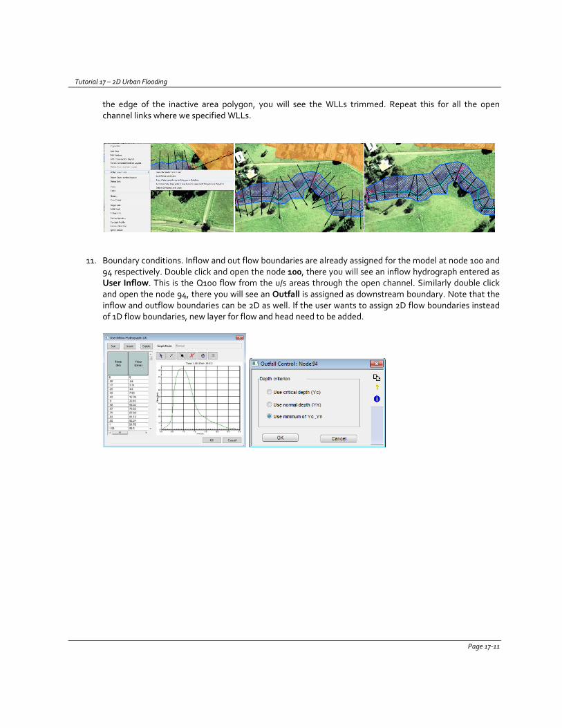
Tutorial 17 – 2D Urban Flooding
the edge of the inactive area polygon, you will see the WLLs trimmed. Repeat this for all the open channel links where we specified WLLs.
11. Boundary conditions. Inflow and out flow boundaries are already assigned for the model at node 100 and 94 respectively. Double click and open the node 100, there you will see an inflow hydrograph entered as User Inflow. This is the Q100 flow from the u/s areas through the open channel. Similarly double click and open the node 94, there you will see an Outfall is assigned as downstream boundary. Note that the inflow and outflow boundaries can be 2D as well. If the user wants to assign 2D flow boundaries instead of 1D flow boundaries, new layer for flow and head need to be added.
Page 17-11
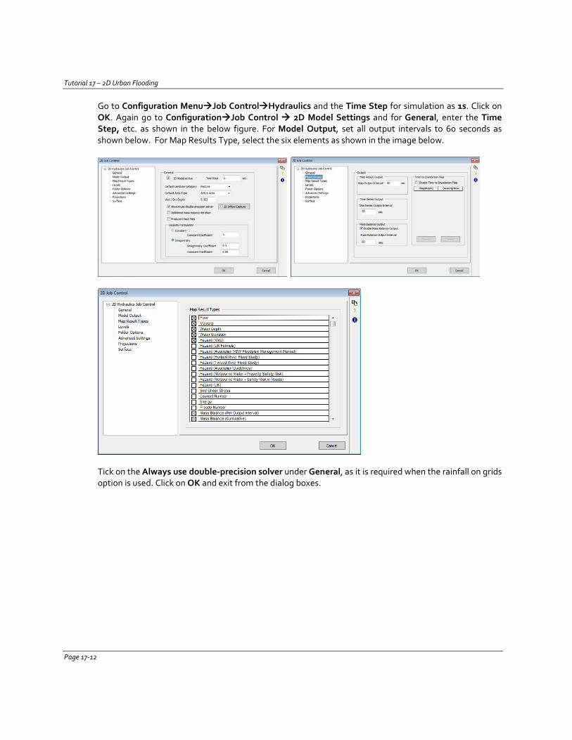
Tutorial 17 – 2D Urban Flooding
Go to Configuration MenuJob ControlHydraulics and the Time Step for simulation as 1s. Click on OK. Again go to ConfigurationJob Control 2D Model Settings and for General, enter the Time Step, etc. as shown in the below figure. For Model Output, set all output intervals to 60 seconds as shown below. For Map Results Type, select the six elements as shown in the image below.
Tick on the Always use double-precision solver under General, as it is required when the rainfall on grids option is used. Click on OK and exit from the dialog boxes.
Page 17-12
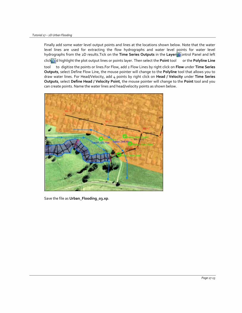
Tutorial 17 – 2D Urban Flooding
Finally add some water level output points and lines at the locations shown below. Note that the water level lines are used for extracting the flow hydrographs and water level points for water level hydrographs from the 2D results.Tick on the Time Series Outputs in the Layers Control Panel and left
click and highlight the plot output lines or points layer. Then select the Point tool or the Polyline Line
tool to digitize the points or lines.For Flow, add 2 Flow Lines by right click on Flow under Time Series Outputs, select Define Flow Line, the mouse pointer will change to the Polyline tool that allows you to draw water lines. For Head/Velocity, add 4 points by right click on Head / Velocity under Time Series Outputs, select Define Head / Velocity Point, the mouse pointer will change to the Point tool and you can create points. Name the water lines and head/velocity points as shown below.
Save the file as Urban_Flooding_03.xp.
Page 17-13
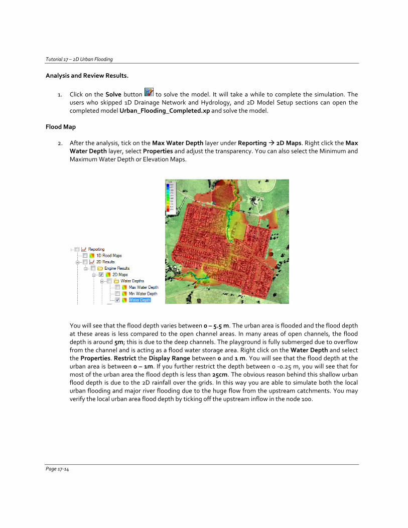
Tutorial 17 – 2D Urban Flooding
Analysis and Review Results.
1. Click on the Solve button to solve the model. It will take a while to complete the simulation. The users who skipped 1D Drainage Network and Hydrology, and 2D Model Setup sections can open the completed model Urban_Flooding_Completed.xp and solve the model.
Flood Map
2. After the analysis, tick on the Max Water Depth layer under Reporting 2D Maps. Right click the Max Water Depth layer, select Properties and adjust the transparency. You can also select the Minimum and Maximum Water Depth or Elevation Maps.
You will see that the flood depth varies between 0 – 5.5 m. The urban area is flooded and the flood depth at these areas is less compared to the open channel areas. In many areas of open channels, the flood depth is around 5m; this is due to the deep channels. The playground is fully submerged due to overflow from the channel and is acting as a flood water storage area. Right click on the Water Depth and select the Properties. Restrict the Display Range between 0 and 1 m. You will see that the flood depth at the urban area is between 0 – 1m. If you further restrict the depth between 0 -0.25 m, you will see that for most of the urban area the flood depth is less than 25cm. The obvious reason behind this shallow urban flood depth is due to the 2D rainfall over the grids. In this way you are able to simulate both the local urban flooding and major river flooding due to the huge flow from the upstream catchments. You may verify the local urban area flood depth by ticking off the upstream inflow in the node 100.
Page 17-14
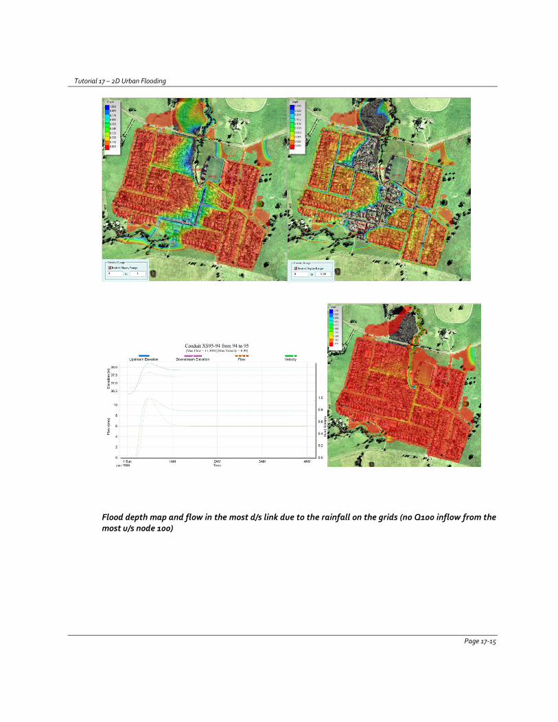
Tutorial 17 – 2D Urban Flooding
Flood depth map and flow in the most d/s link due to the rainfall on the grids (no Q100 inflow from the most u/s node 100)
Page 17-15
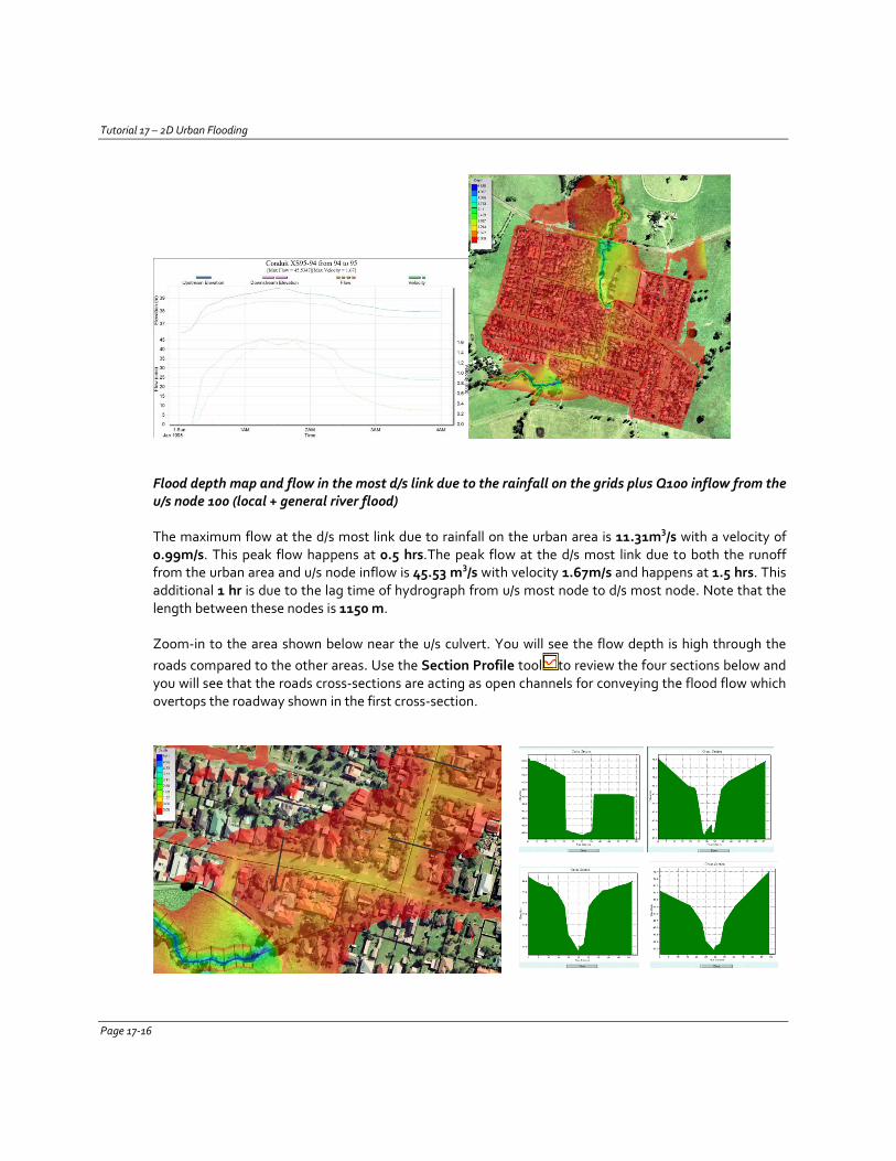
Tutorial 17 – 2D Urban Flooding
Flood depth map and flow in the most d/s link due to the rainfall on the grids plus Q100 inflow from the u/s node 100 (local + general river flood)
The maximum flow at the d/s most link due to rainfall on the urban area is 11.31m3/s with a velocity of 0.99m/s. This peak flow happens at 0.5 hrs.The peak flow at the d/s most link due to both the runoff from the urban area and u/s node inflow is 45.53 m3/s with velocity 1.67m/s and happens at 1.5 hrs. This additional 1 hr is due to the lag time of hydrograph from u/s most node to d/s most node. Note that the length between these nodes is 1150 m.
Zoom-in to the area shown below near the u/s culvert. You will see the flow depth is high through the roads compared to the other areas. Use the Section Profile tool to review the four sections below and you will see that the roads cross-sections are acting as open channels for conveying the flood flow which overtops the roadway shown in the first cross-section.
Page 17-16

Tutorial 17 – 2D Urban Flooding
Upstream Culvert
3. Zoom-in further to view the u/s most culvert clearly and tick on the 2D Vectors (Flows) under the Reporting layer. You may right click on this 2D Vectors layer and adjust the flow arrows etc.
You will see from the flow vectors that flow is getting stagnant near the u/s of the culvert. This is due to the limited conveyance of the culvert barrels and downstream condition together. The culvert is box type with 1.8m x 1.8m and 3 barrels. Right click on the plot output line Culvert_U/S_Flow and select the Graph option. You will see the flow hydrographs at the u/s and d/s of the culvert together. The peak flow at the u/s and d/s are 91 and 66 m3/s respectively and happens at 1 hr. Note that the remaining flow is conveyed through the culvert barrels to the connected drainage pipes.Click on the Close button, select the culvert link and click on Review Results button. The peak flow through the culvert is 44.47 m3/s. The peak velocity of flow is 3.88 m/s which might be a bit high for a concrete culvert to carry safely. You will see a sudden dip in the flow and velocity at 1.06 hrs and at the same time a raise in the d/s water level. This is due to the overtopping flow through the road embankment. Click on the water level point and review Road_Overtop and Culvert1_Road_Depth.
Page 17-17
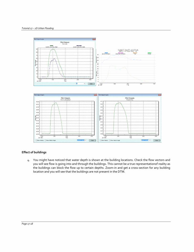
Tutorial 17 – 2D Urban Flooding
Effect of buildings
4. You might have noticed that water depth is shown at the building locations. Check the flow vectors and you will see flow is going into and through the buildings. This cannot be a true representationof reality as the buildings can block the flow up to certain depths. Zoom-in and get a cross-section for any building location and you will see that the buildings are not present in the DTM.
Page 17-18
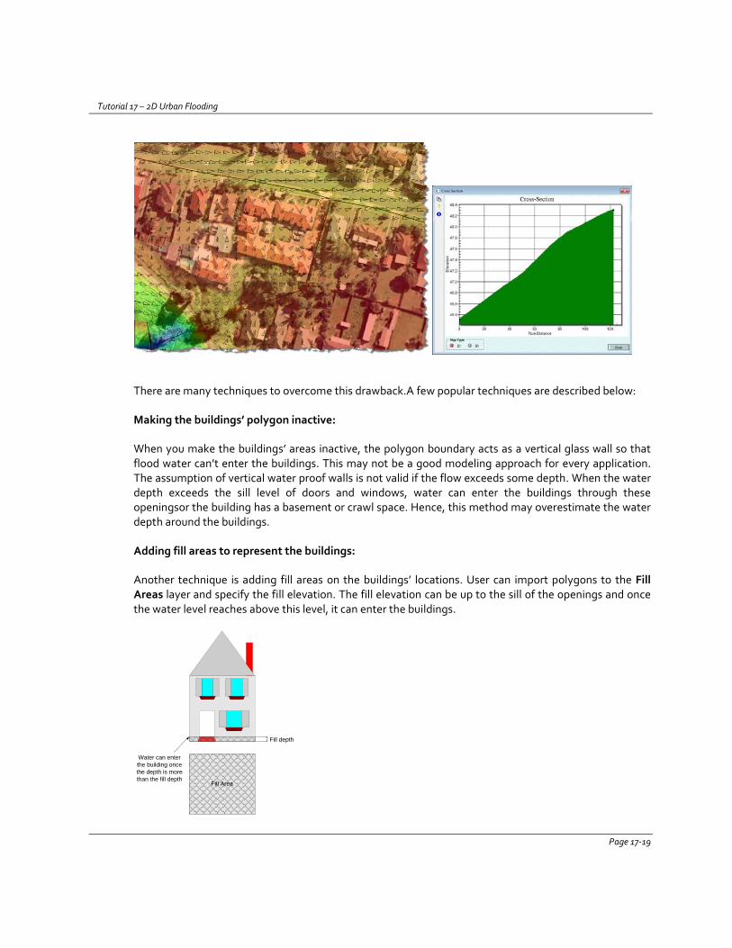
Tutorial 17 – 2D Urban Flooding
There are many techniques to overcome this drawback.A few popular techniques are described below:
Making the buildings’ polygon inactive:
When you make the buildings’ areas inactive, the polygon boundary acts as a vertical glass wall so that flood water can’t enter the buildings. This may not be a good modeling approach for every application. The assumption of vertical water proof walls is not valid if the flow exceeds some depth. When the water depth exceeds the sill level of doors and windows, water can enter the buildings through these openingsor the building has a basement or crawl space. Hence, this method may overestimate the water depth around the buildings.
Adding fill areas to represent the buildings:
Another technique is adding fill areas on the buildings’ locations. User can import polygons to the Fill Areas layer and specify the fill elevation. The fill elevation can be up to the sill of the openings and once the water level reaches above this level, it can enter the buildings.
Fill Area
Fill depth
Water can enter the building once the depth is more than the fill depth
Page 17-19
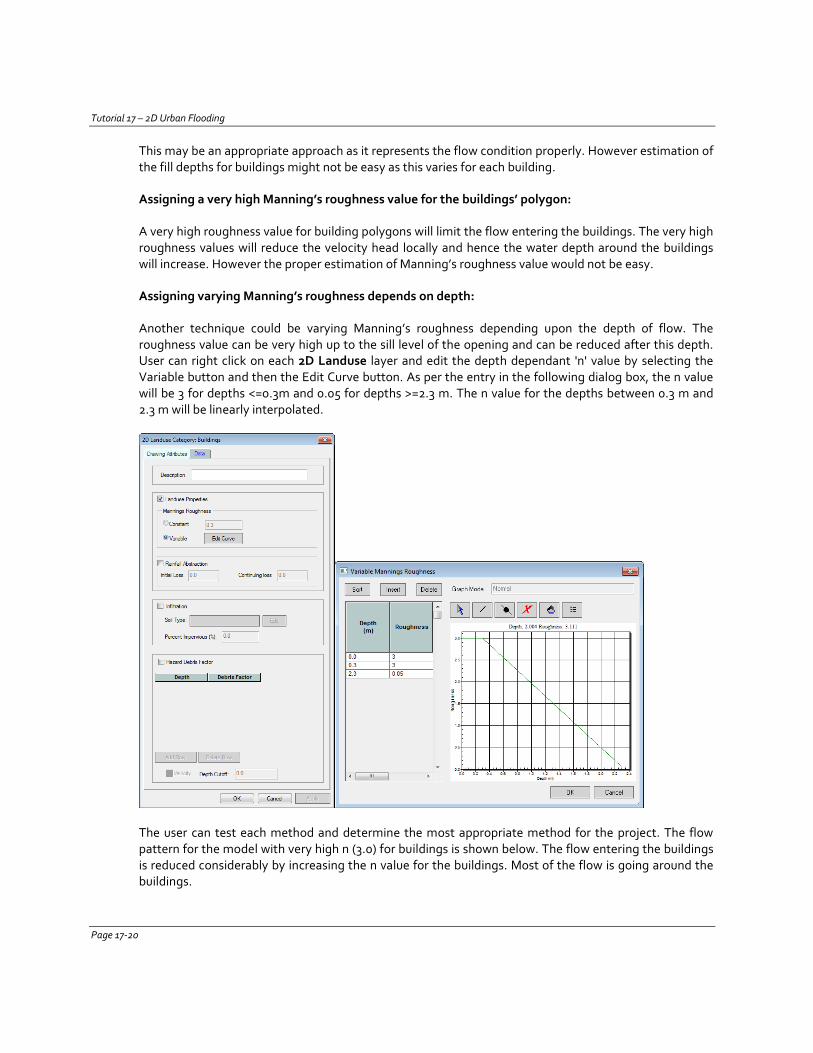
Tutorial 17 – 2D Urban Flooding
This may be an appropriate approach as it represents the flow condition properly. However estimation of the fill depths for buildings might not be easy as this varies for each building.
Assigning a very high Manning’s roughness value for the buildings’ polygon:
A very high roughness value for building polygons will limit the flow entering the buildings. The very high roughness values will reduce the velocity head locally and hence the water depth around the buildings will increase. However the proper estimation of Manning’s roughness value would not be easy.
Assigning varying Manning’s roughness depends on depth:
Another technique could be varying Manning’s roughness depending upon the depth of flow. The roughness value can be very high up to the sill level of the opening and can be reduced after this depth. User can right click on each 2D Landuse layer and edit the depth dependant 'n' value by selecting the Variable button and then the Edit Curve button. As per the entry in the following dialog box, the n value will be 3 for depths <=0.3m and 0.05 for depths >=2.3 m. The n value for the depths between 0.3 m and 2.3 m will be linearly interpolated.
The user can test each method and determine the most appropriate method for the project. The flow pattern for the model with very high n (3.0) for buildings is shown below. The flow entering the buildings is reduced considerably by increasing the n value for the buildings. Most of the flow is going around the buildings.
Page 17-20
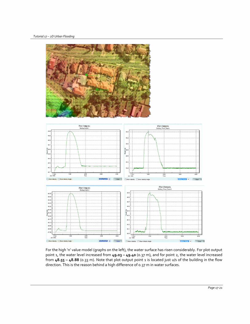
Tutorial 17 – 2D Urban Flooding
For the high ‘n’ value model (graphs on the left), the water surface has risen considerably. For plot output point 1, the water level increased from 49.03 – 49.40 (0.37 m), and for point 2, the water level increased from 48.55 – 48.88 (0.33 m). Note that plot output point 1 is located just u/s of the building in the flow direction. This is the reason behind a high difference of 0.37 m in water surfaces.
Page 17-21
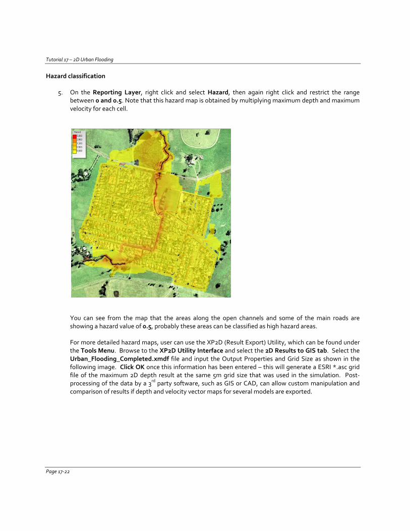
Tutorial 17 – 2D Urban Flooding
Hazard classification
5. On the Reporting Layer, right click and select Hazard, then again right click and restrict the range between 0 and 0.5. Note that this hazard map is obtained by multiplying maximum depth and maximum velocity for each cell.
You can see from the map that the areas along the open channels and some of the main roads are showing a hazard value of 0.5, probably these areas can be classified as high hazard areas.
For more detailed hazard maps, user can use the XP2D (Result Export) Utility, which can be found under the Tools Menu. Browse to the XP2D Utility Interface and select the 2D Results to GIS tab. Select the Urban_Flooding_Completed.xmdf file and input the Output Properties and Grid Size as shown in the following image. Click OK once this information has been entered – this will generate a ESRI *.asc grid file of the maximum 2D depth result at the same 5m grid size that was used in the simulation. Post-processing of the data by a 3rd party software, such as GIS or CAD, can allow custom manipulation and comparison of results if depth and velocity vector maps for several models are exported.
Page 17-22

Tutorial 17 – 2D Urban Flooding
Mitigation option:
6. The manhole/pit overflows are due to the less conveyance of the drainage pipes. The easiest way to tackle this issue is to increase the conveyance of the drainage pipes. However, this increased conveyance will create more flood in the d/s channel overbanks.
As huge inflow is coming from the u/s during a 100 yr-30min design event, the designed drainage system is unable to carry the flow to downstream due to less conveyance. An upstream detention is the most obvious solution in this case. A model with detention pond at upstream area is completed. Open the model Urban_Flooding_Completed_Pond.xp.
The detention pond is made using the Fill Areas option under the Topography layer. The below table shows the storage characteristics of the pond:
Elevation (m) Waterspread Area (Ha)43 1.9445 2.7447 3.6848 4.8449 6.06
Page 17-23
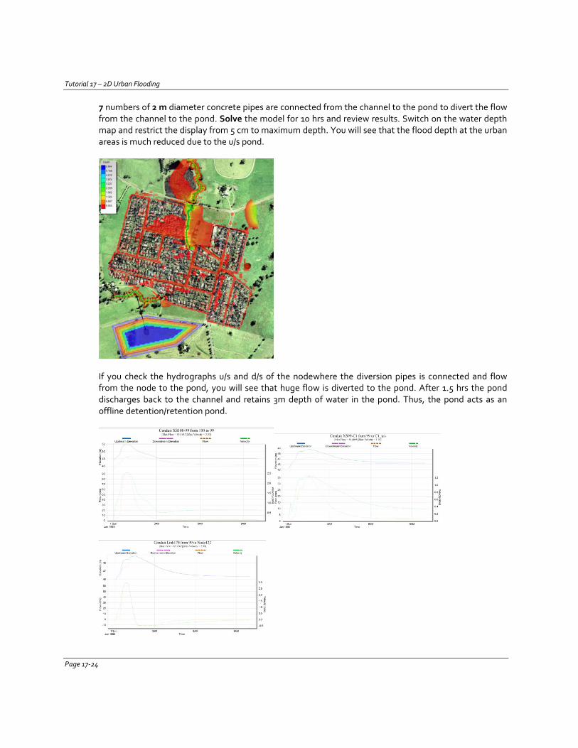
Tutorial 17 – 2D Urban Flooding
7 numbers of 2 m diameter concrete pipes are connected from the channel to the pond to divert the flow from the channel to the pond. Solve the model for 10 hrs and review results. Switch on the water depth map and restrict the display from 5 cm to maximum depth. You will see that the flood depth at the urban areas is much reduced due to the u/s pond.
If you check the hydrographs u/s and d/s of the nodewhere the diversion pipes is connected and flow from the node to the pond, you will see that huge flow is diverted to the pond. After 1.5 hrs the pond discharges back to the channel and retains 3m depth of water in the pond. Thus, the pond acts as an offline detention/retention pond.
Page 17-24


![Skaffold - storage.googleapis.com · [getting-started getting-started] Hello world! [getting-started getting-started] Hello world! [getting-started getting-started] Hello world! 5.](https://static.fdocuments.net/doc/165x107/5ec939f2a76a033f091c5ac7/skaffold-getting-started-getting-started-hello-world-getting-started-getting-started.jpg)