1

Getting Stable: An Evaluation of the Incentives for

Permanent Contracts in Italy*

This version: June 2014

Emanuele Cianiab†

and Guido de Blasioc

a Bank of Italy, Regional Economic Research Division - Florence Branch, via dell’Oriuolo 37/39, 50122 Firenze, Italy

b Centre for the Analysis of Public Policies, University of Modena and Reggio Emilia, viale Berengario 51, 41121

Modena, Italy

c Bank of Italy, Structural Economic Analysis Directorate, via Nazionale 91, 00184 Roma, Italy

Abstract

There is little evidence about the effectiveness of incentives for the conversion of fixed-term

contracts into permanent jobs. We aim at filling this gap by studying a recent Italian program,

which provides benefits to employers who convert contracts for workers in specific demographic

groups (females, younger men). Due to binding funding constraints, the incentives were available

only for few days, allowing us to employ a difference-in-differences strategy between very similar

short periods of time. By using high-quality administrative microdata for the region of Veneto, we

show that the subsidy increased conversions by 83% on average, with no evidence of substitution

effects over time or across groups of workers.

JEL: J21, J41, J48

Keywords: fixed-term contracts, permanent employment, diff-in-diffs

* We wish to thank Bruno Anastasia and the staff at Veneto Lavoro (in particular Sebastiano Basso) for granting us

access to the dataset and for providing excellent support in understanding its technicalities. We are also indebted to

Anna Giraldo, Adriano Paggiaro, Sauro Mocetti, Eliana Viviano, Massimo Gallo, Andrea Petrella, Paolo Sestito and

seminar participants at Veneto Lavoro, University of Milan and at the Bank of Italy for useful comments and critiques.

All remaining errors are ours. The views expressed in this paper are those of the authors and do not necessarily reflect

those of the Bank of Italy. † Corresponding author: Tel.: +39 055 2493320

E-mail addresses: emanuele.ciani@bancaditalia.it (E. Ciani), guido.deblasio@bancaditalia.it (G. de Blasio).

2

1. Introduction

In the process of reforming the labor market institutions, a government faces a trade-off between

the need of increasing labor market flexibility and the desire to guarantee some level of stability to

individual workers. On the one hand, the use of fixed-term contracts might bring about efficiency

gains. Apart from technological reasons (buffer stock, temporary substitutions, seasonal jobs; see

Cappellari et al., 2012), employers can use short-term appointments to increase employees’

productivity, by both inducing workers to exert more effort (Engellandt and Riphahn, 2005) and

screening them before a permanent hire in order to avoid mismatches. From the worker’s point of

view, fixed-term contracts may be preferable when the individual is in the process of choosing

his/her best occupation, or for workers who are less interested in investing into job-specific human

capital (Booth et al., 2002). On the other hand, a widespread use of temporary contracts may

increase job-insecurity, therefore affecting the welfare of the workers and their choices. For

instance, empirical evidence suggests that job-insecurity may have negative effects on youth

emancipation (Becker et al., 2010) and fertility (Modena and Sabatini, 2012; Priftin and Vuri,

2013). On related grounds, temporary contracts are generally associated with a reduced level of

training (Arulampalam and Booth, 1998; Arulampalam et al., 2004), and therefore with less chances

to increase workers’ human capital. Clearly, these disadvantages are likely to be more problematic

if individuals experience a series of temporary jobs without access to a permanent one.

A government may wish to regulate the use of fixed-term contracts in order to maximize the

difference between the advantages of more flexibility and the costs of job-insecurity. In doing so, it

faces relevant constraints. Temporary workers are generally less expensive for firms, because of

both smaller social contributions and a less stringent employment protection legislation (EPL).

Therefore, making these arrangements more costly might jeopardize fixed-term hiring. By the same

token, it can be politically unfeasible to reduce the cost of permanent contracts, which are

overwhelmingly protected by trade unions.

One possible way to increase the proportion of stable jobs would be to subsidize direct hires

with a permanent contract. This incentive is likely to reduce the inflow of temporary workers and

increase the one of long-term employees. However, the subsidy is also likely to diminish the

efficiency gains related to the use of flexible contracts. A different solution would be to subsidize

employers for conversions from fixed-term to open-end contracts. This scheme allows them to

freely hire temporary workers, possibly generating the efficiency gains related to greater flexibility,

but at the same time reducing the risk that individuals incur in a series of fixed-term contracts.

Given the information asymmetry between workers and potential employers, an incentive for

3

contract conversion may be more effective than one for direct hires, because it exploits the

preference of employers to sign permanent contracts with workers that have already been screened.

In this paper we evaluate the effectiveness of a program that provides monetary incentives for

conversions. The ability of a program of this type to reach the stated target should not be taken for

granted: employers will turn a position into permanent only if the subsidy is sufficiently generous to

compensate the relative gains of keeping it as temporary. In the booming literature on policy

evaluation of labor market schemes, the assessment of conversion programs seems to be rather

scarce. The available evidence mostly refers to policies that either increased the cost of fixed term

contracts or made it cheaper to hire on a permanent basis (for instance, Hernanz et al., 2003; Maurin

and Michaud, 2004; Mendéz, 2013). Only few studies (Cipollone and Guelfi, 2003, 2006; Battiloro

and Costabella, 2011) evaluated incentives which also applied to the conversion of fixed-term

positions.1

In this paper we contribute to the literature by providing evidence from Italy on a scheme that

subsidized conversion from temporary to open-end contracts, the Decree 5 October 2012. The

policy did not apply to all groups of workers, as it excluded men aged 30 or more. Furthermore, the

funds were limited; as a matter of facts, they were exhausted in a couple of weeks. We elaborate on

these features of the scheme and evaluate its effects through a diff-in-diffs strategy, which compares

eligible workers with their non-eligible counterparts (older males) over very short periods of time.

Using aggregate time series from the Veneto region, Anastasia et al (2013) showed that for the

eligible groups the total number of conversions approximately doubled over the period of validity of

the policy with respect to the previous year, and that there was a significant difference between the

totals for men aged 29 and men aged 30. Differently from them, we directly use the microdata built

from the administrative archives of the same region, a dataset that allows us to track individual

fixed-term contracts over time. We focus on how their probability of conversion changed over

different periods within 2012. In particular, we distinguish between periods with different exposure

to the effects of the scheme (pre-announcement, announcement, treatment, end of funds). Our

estimates suggest that the policy increased the probability of transformation by 83% with respect to

the counterfactual rate of conversion, with larger effects for men under 30 and women over 30 and

smaller impact on younger women. There is no evidence that entrepreneurs postponed conversions

during the short period between the announcement and the full implementation of the program, nor

that they reduced the conversion rate after the funds were terminated; we also fail to find evidence

that the impact is due to substitution between eligible and non-eligible workers. These results are

1 Portugal introduced, in 2002, a scheme of incentives for the conversion of temporary contracts, but to the best of our

knowledge no study has evaluated its effects.

4

robust to several checks, including a falsification exercise aimed at detecting infra-annual

confounding trends. We finally show that the effect seems to have lasted during the eight months

after the end of the policy, which is the time extension of the last available data at the moment of

writing.

The paper is structured as follows. Section 2 briefly summarizes the related literature. Section 3

outlines the policy. Section 4 presents the data, while Section 5 describes the identification strategy.

Section 6 discusses the results. Section 7 compares the scheme with two other similar policies from

Italy, to tentatively draw some conclusions for program design.

2. Previous literature

Only a few papers study the effect of programs aimed at modifying the relative profitability of

short-term vs open-end arrangements. Hernanz et al (2003) evaluate a Spanish reform in 1997 that

reduced the cost of open-end contracts. They find a positive effect on flows to permanent jobs.

Mendéz (2013) criticize their results, by claiming that their assumption that individuals aged

between 30 and 45 could not be hired with the new open-end contracts is not correct, because they

could if they had been previously hired as fixed-term workers. Using a different method and

evaluating also a previous reform that restricted the use of fixed-term contracts (1994), he provides

evidence suggesting that the conversion rate did not increase. Maurin and Michaud (2004) focus on

France, where a reform in 2002 increased the cost of terminating a temporary contract instead of

converting it into a permanent one. Compared to a subsidy for conversion, this measure also implies

an extra-cost in hiring individuals with a fixed-term contract. The authors provide evidence of an

increase in the proportion of temporary contracts converted into permanent ones, but they also find

that the higher costs induced a decrease in the number of new fixed-term hires and therefore a

contraction in the overall employment. More related to our investigation, an Italian program in 2001

provided employers with incentives for hires or conversions with a permanent contract, but

conditional on increasing the total workforce of the firm. Cipollone and Guelfi (2003, 2006) find

evidence of no aggregate effects, although the results were highly heterogeneous by education and

previous employment condition. Battiloro and Costabella (2011) evaluate a subsidy of around 4,500

euros for conversions, that was introduced in 2007 in the Province of Turin in Italy. By comparing

the time series in Turin with those from other unaffected provinces, they find no evidence of an

increase in the number of conversions.

Our contribution is also related to two other streams of literature. The first one refers to the

effects of EPL on job flows. Indeed, the incentives set out by the Decree 5 October 2012 were

introduced to compensate the firms for the higher cost of permanent contracts. Several studies

5

exploit an Italian reform in 1990 that increased the level of EPL for permanent workers in small

firms. Their main finding suggest that higher EPL decreases both accessions and separations,

consistently with theoretical predictions (Bertola, 1990; Boeri and Jimeno, 2005; Kugler and Pica,

2008). A stronger protection for permanent workers increases their relative cost with respect to

temporary employees: Grassi (2009) uses administrative data from Italy and provides evidence that

the more stringent EPL induced by the reform reduced the rate of conversion from fixed-term to

permanent contracts. Similarly, Schivardi and Torrini (2008) show that larger firms, to which higher

EPL applies, tend to make more use of flexible workers.

The other related stream of literature is the one which focuses on the stepping stone effect

(Booth et al., 2002); that is, on the ability of short-term appointments to promote the access to

permanent employment. Empirically, this literature studies the probability that individuals with a

fixed-term contract at a certain point in time are employed on a permanent basis later on, and

compares them with individuals who were instead unemployed. Booth et al. (2002) find that in the

UK standard fixed-term positions lead to permanent jobs later in time. In Italy, the available

evidence supports the idea of the stepping stone effect (Ichino et al., 2005; Picchio, 2008; Barbieri

and Sestito, 2008; Bruno et al., 2012), although results are highly heterogeneous by type of

temporary contract (Berton et al, 2011). Our paper analyze how a subsidy can affect the rate of

conversion of temporary contracts into permanent ones; that is, how public money may help the

stepping stone effect to take place.

3. The program

The Decree 5 October 2012 introduced financial incentives for employers who:

converted temporary contracts for eligible workers into permanent ones; the incentive in this

case was equal to 12,000 euros per conversion;

stabilized workers holding non-standard contracts (parasubordinati) or who had concluded a

temporary contract in the previous 6 months and had been unemployed thereafter; similarly

this incentive amounted to 12,000 euros per stabilization;

hired workers with a temporary contract, but only if this hire increased the total workforce

of the firm. In this case the benefit was between 3,000 and 6,000 euros depending on the

length of the contract.

6

The scheme required that the job lasted for at least 6 months after the conversion/hire.2 Eligible

workers were men aged less than 30, and women of any age. In case of permanent contracts on a

part-time base, the amount of the subsidy was proportionally reduced. Moreover, each employer

could request at most 10 incentives.

The Decree made use of a dedicated national fund for the increase in the employment of youth

and women. The fund was set up by law 201/2011 (December 2011), but details on how the money

would have been used were not fully defined until 5 October 2012, when the Decree introducing the

program was approved by the Ministry of Labor and Social Policies jointly with the Ministry of

Economics and Finance. We therefore take the latter as the date of announcement of the program.

Figure 1 depicts the timeline of the policy.

Figure 1 Timeline of the policy

The incentive applied only to conversions/stabilizations/hires starting from the official date of

publication of the Decree: the 17th

of October. The program was supposed to be in place up to the

31st of March 2013. At the moment of the formal request, the firms should had already signed (and

communicated to the competent administration) the new contract with the eligible worker. Given

that funds were limited, employers were allowed to check online, at the time of the application,

whether the number of requests made until then was already sufficient to exhaust the total budget.

However, if the funds terminated on the day of application, demands would have been funded on a

first-come-first-served basis. The 2nd

of November the National Institute for Social Security (INPS)

communicated that the number of requests received until then was enough to terminate the funds

and, therefore, the agency discouraged new requests. Some requests arrived after the 2nd

of

November. This happened because it was uncertain whether all the demands already presented were

actually eligible. Therefore, some employers might have applied, notwithstanding the INPS

warning, hoping that they could have still benefited from funding.

2 Note that the program did not introduced any constraint as to the variation in total workforce following the

conversions/stabilizations.

7

The only publicly available data on the program come from the website of the Ministry of

Labor: at the national level, between 17/10/2012 and 31/03/2013, 44,054 requests were made, of

which only 24,581 were accepted.3 The decision on the acceptance was communicated to the firms

only in June 2013, to comply with the requirement that the job had lasted at least 6 months. Given

that the rules of the game were relatively simple, the selection of requests was mostly based on the

order of presentation, rather than on their eligibility compliance.

From the information released by the Ministry of Labor we know that around 90% of all

incentives was distributed for conversions or stabilizations of temporary contracts. Considering that

the incentive for direct hires with temporary contracts was less generous (and required an increase

in the overall workforce), it is not surprising that few requests were made for that option. Compared

to temporary workers, the number of parasubordinati is much smaller; moreover, this group is

highly heterogeneous as for the features of the firm-employee relation. For these reasons in this

paper we focus on temporary contract conversions only. We do not consider those who had

concluded a temporary contract within 6 months and had been unemployed thereafter. The main

issue is that these individuals may also migrate to/from other regions and therefore we do not

always observe whether they are subject to a stabilization. Nevertheless, in the robustness section

we show that there is no evidence of changes in the number of direct hires during the validity of the

incentives.

4. Data

Since March 2008 employers who hire new workers or make alterations to pre-existing contracts

are obliged to communicate it to a regional agency through an online system, named sistema di

comunicazione obbligatoria (Anastasia et al., 2009, 2010). This administrative archive does not

provide the complete stock of workers, given that permanent contracts signed before March 2008

do not enter it. However, the archive allows researchers to track the universe of job relationships

that started with a temporary contract after March 2008. Considering that standard fixed-term

contracts can be signed only for up to 36 months, their entire stock should be observable in the files

starting from March 2011.4

The quality of these data depends not only on the accuracy of the employers, but also on the

skills of the regional agencies in charge of maintaining and validating the archives. In Italy, the

region with the longest tradition in analyzing these data is Veneto (Maurizio, 2006), where the local

3 http://www.lavoro.gov.it/Notizie/Pages/20130610_Incentivi_giovani_donne.aspx (last retrieved: 20/01/2014).

4 There are few exceptions that involve a small number of workers, in particular contracts for directors that could be

signed for 5 years. However, our data are based on a region that was already collecting the data from several years

before 2008, and therefore we should be able to observe almost all relevant contracts in 2011 and 2012.

8

agency (Veneto Lavoro) started elaborating a dedicated software since 1996. Moreover, using the

flow of the communications, the agency organizes a full set of longitudinal microdata that track

single individuals through time. Veneto Lavoro makes available to researchers the entire universe of

microdata, while at the national level these data are available only for a subset of workers

(individuals born in 48 different dates) and, crucially, without any information about contract

conversions. The region of Veneto is one of the most important economic area of the country:

according to the Labor Force Survey, in 2012 Veneto accounted for 9.5% of total employees in

Italy, and for the 8.3% of total employees on a temporary contract.

We focus on the (regional) universe of job relationships that started with a standard temporary

contract (tempo determinato) and were still active as temporary during 2012. These relationships

might either keep their short-term nature, or be converted into permanent positions. We analyze the

extent to which there was a change in the event “temporary contract converted into permanent”

because of the program. We select only standard temporary contracts; that is, we exclude contracts

that are activated to substitute a permanent worker on leave (per sostituzione), signed with a

temporary employment agency (interinale o a scopo di somministrazione), allowing the employee

to work in her own place (a domicilio), and designed for particular sectors or for other particular

reasons.5 We do very minor corrections on the raw data, dropping few cases where we observed a

change in the nature of the contract without an explicit reason and correcting the date of conversion

for some job-relationships where the conversion episode was repeated more than once. We also

exclude very few cases (around 0.6% of those job-relationships that were subject to conversions)

where the standard temporary contract was converted into a non-standard permanent contract,

because it may signal measurement error.

Using the longitudinal information on each job relationship i=1,…,N we build a panel over four

different periods t=1,…,4 in 2012. Each period has a length between 12 and 16 days (the next

Section explains the details on these units of time). For each period, we keep only job-relationships

that are active; that is, temporary contracts with at least one day of duration. The panel is

unbalanced for two reasons: a) new temporary contracts can be signed during the year; therefore

new job relationships can enter the panel in any period; b) temporary contracts terminate (either for

5 This selection clears possible distortions generated by the specificity of these contracts. Among eligible fixed term

workers in the selected periods in 2012, 71.9% had standard contracts, and they represented 90.7% of the contracts that

were converted into permanent. Our main results carry through to the more general case, where all these nonstandard

contracts are kept into the dataset (apart from those signed with a temporary employment agency which were not

eligible for the incentive); in this case the point estimate is smaller, but it is quite close to our main results if measured

as a proportion of the counterfactual. Our findings are also undistinguishable if the public sector is dropped from the

sample. All these sets of results are available on request.

9

the natural end of the contract or for other reasons) or are converted into permanent ones; these

contracts exit the panel the period after that in which the event takes place.

Our main outcome is a binary variable:

yit = 1[job-relationship i is converted from temporary to permanent in period t] (1)

so that our results have to be interpreted as the impact of the scheme on the probability that a

temporary contract active during a single period t is converted into permanent during the same

period.

For each job-relationship we observe some time invariant characteristics: educational level of

the worker, gender, sector of activity and citizenship.6 We also know two important time variant

observables: the worker’s age at the start of each period and the job-relationship duration at the end

of the period.7 Finally, we can identify the employer: this allows us to cluster the standard errors at

the firm level and observe how many temporary contracts are referred to the same firm, in a

particular moment in time.

From the panel, we drop those observations with missing age or gender (21 in total), and we

select only individuals aged between 16 and 65, mainly in order to avoid extreme cases that are

likely to signal measurement error. We end up with 593,028 observations, approximately 148

thousand job relationships per period.

5. Identification strategy

We use a diff-in-diffs strategy over different periods within 2012 and different groups in terms

of terms of program eligibility, defined on the basis of demographic characteristics. We focus on

the effect of the policy on the eligible groups conversion rate, so that our estimates can be

interpreted as the Intention To Treat (ITT). This is the effect of interest for a policy maker who

wants to understand the overall impact of the program. Our data do not contain information on who

actually received the incentive. Nevertheless, in Section 6 we also calculate the actual cost for each

increased unit of conversion in a scenario in which all transformations for the eligible groups are

incentivized.

Following the standard model (Angrist and Pischke, 2009), we assume that the expected

potential outcome when not treated (indexed by 0) depends additively on the group g and on the

period t:

6 We use the information on the educational level in the most recent communication regarding the temporary contract

(before the conversion, in case it takes place). 7 We censor to 5 years 0.5% of the observations who have longer duration.

10

E[y0igt | g, t] = μg + λt (2)

which implies two basic assumptions (Blundell and MaCurdy, 1999):

A1. The time trend is parallel across groups.

A2. The group effect does not change over time, that is the group composition is (on

average) constant.

Secondly, we assume that the effect of the policy is additive, so that the potential outcome when

treated (indexed by 1) is simply

E[y1igt | g, t] = E[y0igt | g, t] + δ= μg + λt+ δ. (3)

Exploiting the timeline of the policy (see Figure 1) we define 4 periods of interest:

Period I: [19/09 - 4/10]; that is, 16 days before the announcement.

Period II: [5/10 - 16/10]; that is, the 12 days between announcement and the actual start

of the program.

Period III: [17/10 - 01/11]; that is, the 16 days when the incentives were fully available.

Period IV: [02/11 - 17/11]; that is, the 16 days after INPS declared that funds were

(presumably) already finished.

We assume that in Period I the policy should not have had any effect: only on the 5th

of October

the scheme of incentives was made public, receiving full attention from the media. Differently,

most of the activity should have taken place in Period III, given that employers already had enough

time to acquire the information. However, the effect of the policy may not be limited to changes

during that period if employers substituted conversions over time in order to benefit from the

incentives.8 To start with, if they were already fully informed during Period II, they may have

postponed some conversions in order to wait for the scheme to be in place. Moreover, the fact that

funds were limited clearly gave them a strong incentive to anticipate in Period III conversions that

would have taken place, without the scheme, much later in time. This is the reason why we also

analyze the days after the shortage of funding (Period IV). In both cases (periods II and IV) we

expect that, if employers substituted conversions over time in order to benefit from the allowances,

the effect of the policy should compensate those observed in Period III. The length of periods I and

IV was chosen in order to match the period of fully validity of the incentives.

8 For a discussion of announcement and implementation effects in diff-in-diffs analysis, see Blundell et al. (2011).

11

The groups entitled for the scheme are defined by the policy: men over 30 were not eligible,

while younger men and women of any age were. We allocate individuals to each group according to

their age at the begin of the period.9

In order to identify the effect δ, we exploit the structure of entitlement envisaged by the policy.

Given that men over 30 were not eligible, we use these workers as a control group to estimate the

trend over periods and then use it to clear the time effects for other groups as well, thanks to

assumption A1. Once we are able to identify λt, we also need to clear out the group effect. In this

case, we exploit the period before the announcement (Period I). If, as we argued, the policy could

not have any effect at that time, then during that period we observe only y0 for everyone, and

therefore we can use it to identify the differences across groups. Finally, for the eligible workers in

the post-announcement periods (II-III-IV) we observe only the outcome when treated (y1), and

therefore we can remove from it the time and group components to get the policy effect δ.

Our results are derived from a specification where the treatment effect δ varies by period of

treatment (II-III-IV) and across eligible groups. This is equivalent to a series of 2X2 diff-in-diffs

estimates, where the control group is always Men over 30 and the pre-reform period is always

Period I. For each single group (men aged less than 30, women aged less than 30 and women aged

30+) or for all the eligible groups altogether, the effects of interest can be identified from the

coefficients on the interaction terms from the regression:

yit = β0 + βE 1[Eligible]it + βII 1[Period II]it + βIII 1[Period III]it + βIV 1[Period IV]it +

+ δII 1[Eligible]it × 1[PII]it + δIII 1[Eligible]it × 1[PIII]it + δIV 1[Eligible]it × 1[PIV]it + εit (4)

For δ to identify a causal effect, we need to assume that the policy was an exogenous shock, so

that the treated groups were not endogenously chosen among those that would have experienced an

increase in conversion rates in any case. This potential threat seems to be hardly realistic: eligibility

was targeted on workers that were more likely to be hit by the on-going economic crisis.

Furthermore, our estimates are based on relatively short periods of time, next to each other. Hence it

is difficult to think that, in the absence of the policy, their conversion rate would have changed

abruptly only during the 16 days in which incentives were fully available.

There are other threats to identification. First of all, there may be seasonal trends that diverge

across groups. Since we estimate the effect of the scheme for very short periods of time during Fall

2012, group-specific seasonality might unduly confound identification. In the empirical section

9 We also replicated the estimates defining the age as referring to the end of the period, with no sensible changes for the

results.

12

below, we check whether this is the case by running a falsification test using 2011 calendar periods

analogous to the ones we focus on for the year 2012.

Secondly, the panel is unbalanced. This implies that the group composition is not guaranteed to

be stable over time. To lessen this concern, we run the same regressions but adding a large set of

covariates (educational level, sector of activity, citizenship, age at the begin of the period, duration

of the job-relationship at the end of the period), which should differentiate out overtime variations

in group compositions.

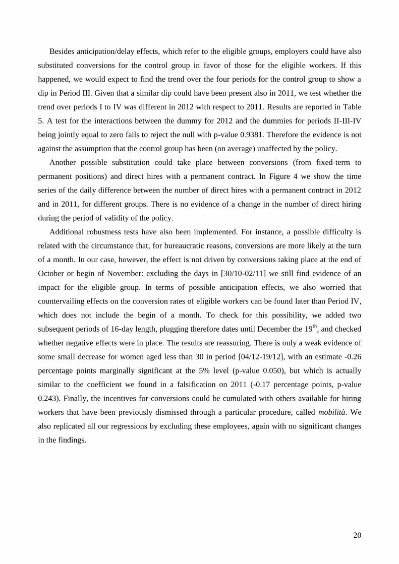
Thirdly, we need to assume that in the Period I employers were not aware of the policy, or at

least that the available information was not enough for them to already change their decisions in

order to later benefit from the incentives. To test this assumption we run a diff-in-diffs regression

that compares the different groups between Period I in 2012 and the analogous period in 2011.

Last but not least, apart from substitution over time, which we directly addressed by looking at

periods II and IV, there may be other reactions that counteracted the effectiveness of the scheme.

The most likely is that the incentives could have induced the employers to favor workers from the

eligible demographic groups and reduce the conversions for the non-eligible (men over 30). We

provide evidence on this potential channel of substitution by looking at the change in the conversion

rate for non-eligible between the same periods in 2012 and the previous year. Furthermore, as a

consequence of the policy, employers could have indirectly subsidized direct hires with permanent

contracts by hiring workers with a temporary one and converting it after few days. Similarly, they

could have favored conversions with respect to direct hires. We also show what happens during the

periods of validity, and relatively to 2011, to the number of jobs starting with a permanent contract.

6. Results

6.1 Main results

Figure 2 shows the rate of conversion for each of the four periods across groups in 2012. Before

the announcement (Period I), the rates of conversion are similar for all groups, with only a slightly

smaller probability for older women. In Period III the probability that a temporary contract becomes

permanent substantially increases for all the eligible groups compared to the non-eligible one. The

jump is larger for younger men. The figure also suggests no signal of substitution effects overtime:

in Period II and Period IV the rates remain quite similar across groups.

13

Figure 2 Probability of conversion from temporary to permanent contract during the period,

by period and group, year 2012

The diff-in-diffs regressions (Table 1) confirm the findings.10

Focusing on the entire group of

the eligible workers, Column (1), there is no evidence of an anticipation effect during the days

between the announcement and the actual date of validity (Period II): although there is a decrease in

the overall conversion rate, this does not diverge across eligible and control groups. Likely,

employers became fully aware of the scheme when the program was about to start, and therefore,

substantial arbitrage across periods was precluded. Differently, there is a significant increase in the

conversion rate by 1.3 percentage points during the 16 days in which incentives were available and

fully funded (Period III).

Our results also document a positive effect of the scheme in Period IV, that is after the day in

which INPS announced that applications were already sufficient to exhaust funds. One possible

explanation is that some employers might have realized that the funds were (probably) terminated

only after having signed a permanent contract with the temporary worker; alternatively, they might

have converted on purpose after the 2nd

of November, in the expectation that some public money

was left for them to benefit (see Section 3).

10

We always use standard errors clustered at the employer level to account for potential common shocks across

different job-relationships. We also tried with standard errors clustered by sector of economic activity: all the main

results on statistical significance carry on.

14

Table 1 Main results (probability of conversion from temporary to permanent contract

during each single period in 2012)

Control group: Men ≥ 30

Dependent variable: dummy for

conversion

(1) (2) (3) (4)

Eligible group:

All eligibles Men < 30 Women < 30 Women ≥ 30

Eligible -0.0021*** -0.0003 -0.0011 -0.0034***

(0.0007) (0.0011) (0.0011) (0.0009)

Period II -0.0123*** -0.0123*** -0.0123*** -0.0123***

(0.0007) (0.0007) (0.0007) (0.0007)

Period III 0.0001 0.0001 0.0001 0.0001

(0.0009) (0.0009) (0.0009) (0.0009)

Period IV -0.0099*** -0.0099*** -0.0099*** -0.0099***

(0.0008) (0.0008) (0.0008) (0.0008)

Eligible × Period II 0.0011 0.0004 0.0000 0.0020**

(0.0008) (0.0012) (0.0013) (0.0010)

Eligible × Period III 0.0130*** 0.0162*** 0.0107*** 0.0124***

(0.0012) (0.0019) (0.0019) (0.0014)

Eligible × Period IV 0.0020** 0.0010 0.0014 0.0027***

(0.0009) (0.0014) (0.0014) (0.0010)

Constant 0.0177*** 0.0177*** 0.0177*** 0.0177***

(0.0007) (0.0007) (0.0007) (0.0007)

Observations 593,028 324,463 304,880 423,177

Note: * p<.10 ** p<.05 *** p<.01. Standard errors clustered for employer in brackets. Estimates are obtained using

StataTM

13. See Figure 1 for the definition of periods.

Columns (2)-(4) document the results for each single group of eligible employees. For workers

under 30 there is evidence of a positive effect of the policy in Period III. The impact is larger for

men and smaller for women. As for the other two periods, there is no statistically significant change

with respect to the control group. For older women we still find a positive effect of the policy in

Period III. However, there is also evidence of a positive effect in periods II and IV; the magnitude is

around 0.2-0.3 percentage points. These findings might suggest a diverging trend for this specific

group, which would violate assumption A1, rather than an actual policy effect. In particular, while

the impact in Period IV can be rationalized on the basis of the scattered timing of the actual end of

the scheme, the effect in Period II is puzzling. If nothing, we would have expected a decrease in the

conversion rate for eligible workers in the time window between announcement and begin of

validity. To take a cautious stance, we might be overestimating the effect of the program for this

specific group. The overestimation should not be a big deal: if we interpolate the observed

diverging trend, the bias would be around 0.2-0.3 percentage points, bringing the effect for women

aged at least 30 closer to that for younger ones.

Table 2 provides some back-of-the-envelope calculations. Given that we do not know who

actually received the incentive, we assume that all eligible conversions in period III were

15

subsidized.11

This gives an upward estimate for the actual cost, because some conversions may have

been excluded from the incentive as a consequence of the shortage of funding. However, this

calculation is still of interest, as it shows the effectiveness of the program in a normal situation

where all eligible conversions receive the subsidy.

Table 2 Summary of the effects

All eligibles Men < 30 Women < 30 Women ≥ 30

Counterfactual conversion rate from

temporary to permanent during period III 0.0157 0.0175 0.0167 0.0145

Reform effect in period III 0.0130 0.0162 0.0107 0.0124

Counterfactual number of conversions during

period III 1,395 402 307 684

Reform effect in number of conversions

during period III 1,156 372 197 589

Reform effect / baseline 83% 92% 64% 86%

% full time on total conversions in period III 62% 84% 56% 50%

Average incentive (euro) 9693 11,047 9,345 9,007

Full cost per increased conversion (euro) 21,392 23,008 23,889 19,472

Note: the number of conversion is calculated as the estimated probability times the number of temporary contracts

active in Period III. The second column does not precisely sum up the following three, because the estimate of the effect

come from the aggregate model (Table 1, col. (1)). The average cost of a conversion is calculated assuming that all part-

time are at half time.

We first compute the proportional increase in conversions due to the program as the ratio

between the estimated effect in Period III and the counterfactual conversion rate predicted by the

model.12

As a share of the counterfactual conversions predicted in Period III, the impact of the

program amounts to 92% for young men, 86% for older women and 64% for females under 30. The

average effect for all the eligible groups is calculated to be 83%. This latter figure implies that in

order to increase the number of conversions by one unit, the government has also financed 1.2

conversions that would have taken place even in the absence of the program. Given that our data

refer to the universe of all temporary contracts (started with a standard type) for workers aged 15-65

in Veneto, we can also compute the effect of the scheme in terms of number of contracts, by

multiplying the number of observations for the estimated probabilities. Among 2,551 conversions

observed in Veneto in Period III, 1,156 of them are attributable to the program. Moreover, using the

information on whether the converted contract is full or part time, we are also able to estimate the

average incentive and the average cost per increased conversion. As reported in Table 2, on average

62% of the job-relationships subject to conversion in Period III were full-time. Assuming that all

11

We also do not know the total amount of incentives that were distributed for conversion that took place in the Veneto

region only and exactly during period III. 12

In the calculation we do not account for the possible presence of an effect in Period IV as well, because it can come

from a diverging trend for older women, and its impact is anyway quite small.

16

the part-times were at half of the standard working time, the average incentive was 9,693 euro.13

This implies that the full cost of an actual unit increase in the number of conversions with respect to

the counterfactual is 21,392 euro, as it requires an expenditure of 11,700 euro on other

transformations that would have taken place even in the absence of the policy.

6.2 Robustness checks

Given that our periods are different both in terms of months and calendar position within the

month, the conversion rate across time might be affected by seasonal patterns. In our case,

seasonality would bias the results only as long as there are group-specific seasonal trends. To check

whether this problem affects our estimates we also replicate the same exercise of Table 1 over the

analogous periods in year 2011, when the scheme was not in place (and no similar policy was

implemented). That is, we run a falsification experiment. From Figure 3, which mirrors Figure 2 but

refers to 2011, we notice no evidence of diverging trends. Table 3 reports the relevant regression

estimates. In Column (1), we find evidence of a small (boundary statistically significant at the 10%

level; p-value 0.095) drop in Period III for the groups of interest, which would either imply that our

results are underestimating the true effect (if the drop would have been there even in the absence of

the policy), or that differential (by groups and periods) shocks to conversion rates materialized.

However, the estimate for Period III in the falsification exercise is quite small compared to the

effect estimated for the same period in 2012, when the policy was effective. If we look at results for

the different eligible groups (columns (2)-(4) in Table 3), the small drop in Period III seems to be

driven only by older women (again the coefficient is significant only at the 10% level). Notice also

that the size of this drop, 0.2 percentage points, would broadly compensate the previously discussed

positive bias for this specific demographic group.14

13

This value is similar to the one that can be obtained dividing the total amount spent in Italy by the total number of

incentives distributed, using the info available on the website of the Ministry of Labour

http://www.lavoro.gov.it/Notizie/Pages/20130610_Incentivi_giovani_donne.aspx (last retrieved: 20/01/2014). 14

One could also combine the falsification over 2011 and the main estimates over 2012 to obtain triple-difference

estimates. We also run this joint regression, obtaining results that are qualitatively similar and support our conclusions.

However, given that in 2011 the interaction terms are generally economically small and not statistically significant, we

prefer to focus on the diff-in-diffs within 2012 in order to avoid introducing noise in our main estimates.

17

Figure 3 Probability of conversion from temporary to permanent contract during the period,

by period and group, year 2011

Table 3 Falsification (probability of conversion from temporary to permanent contract during

each single period in 2011)

Control group: Men ≥ 30

Dependent variable: dummy for

conversion

(1) (2) (3) (4)

All eligibles Men < 30 Women < 30 Women ≥ 30

Eligible -0.0018** -0.0012 -0.0020 -0.0021**

(0.0008) (0.0010) (0.0013) (0.0010)

Period II -0.0121*** -0.0121*** -0.0121*** -0.0121***

(0.0008) (0.0008) (0.0008) (0.0008)

Period III -0.0003 -0.0003 -0.0003 -0.0003

(0.0009) (0.0009) (0.0009) (0.0009)

Period IV -0.0097*** -0.0097*** -0.0097*** -0.0097***

(0.0008) (0.0008) (0.0008) (0.0008)

Eligible × Period II -0.0004 -0.0008 -0.0006 -0.0002

(0.0009) (0.0011) (0.0014) (0.0010)

Eligible × Period III -0.0018* -0.0009 -0.0016 -0.0024*

(0.0011) (0.0014) (0.0018) (0.0013)

Eligible × Period IV -0.0012 -0.0017 -0.0013 -0.0008

(0.0009) (0.0012) (0.0014) (0.0011)

Constant 0.0184*** 0.0184*** 0.0184*** 0.0184***

(0.0007) (0.0007) (0.0007) (0.0007)

Observations 614,895 340,214 313,218 438,457

Note: * p<.10 ** p<.05 *** p<.01. Standard errors clustered for employer in brackets. Estimates are obtained using

StataTM

13. See Figure 1 for the definition of periods.

18

Given that the panel is unbalanced, the group composition is not guaranteed to be stable over

time.15

In order to see whether large changes in the group composition are affecting the results, in

Table 4, column (1) we also add to the basic regression (that of Table 1, Column 1) some relevant

covariates: dummies for sector of activity (ATECO 2 digits), dummies for educational level,

dummy for Italian citizenship, age at the begin of the period, job-relationship duration at the end of

the period.16

The results are basically unchanged. Therefore, overtime variation in group

composition seems not to be driving our findings. Column (2) provides the results we obtain by

adding the covariates to the falsification experiment. The bizarre effect found previously on Period

III is no longer statistically significant.

Table 4 Robustness checks (probability of conversion from temporary to permanent contract

during each single period)

Control group: Men ≥ 30

Treatment group: all eligibles

Dependent variable: dummy for conversion

(1) (2) (3) (4)

Main results

over 2012 with

covariates

Falsification

over 2011with

covariates

Main results

over 2012 with

age [26,34)

Falsification

over 2011 with

age [26,34)

Eligible -0.0017** -0.0008 -0.0004 -0.0023

(0.0008) (0.0008) (0.0015) (0.0016)

Period II -0.0129*** -0.0126*** -0.0140*** -0.0156***

(0.0007) (0.0008) (0.0015) (0.0015)

Period III -0.0009 -0.0012 -0.0008 -0.0012

(0.0009) (0.0009) (0.0019) (0.0019)

Period IV -0.0117*** -0.0112*** -0.0105*** -0.0134***

(0.0008) (0.0008) (0.0017) (0.0016)

Eligible × Period II 0.0014* -0.0003 0.0002 0.0023

(0.0008) (0.0009) (0.0017) (0.0018)

Eligible × Period III 0.0134*** -0.0017 0.0153*** 0.0003

(0.0012) (0.0011) (0.0024) (0.0022)

Eligible × Period IV 0.0026*** -0.0008 0.0000 0.0009

(0.0009) (0.0009) (0.0019) (0.0019)

Constant 0.0405 0.0115*** 0.0193*** 0.0210***

(0.0276) (0.0041) (0.0014) (0.0014)

Observations 593,028 614,895 145,803 156,147

Note: * p<.10 ** p<.05 *** p<.01. Standard errors clustered for employer in brackets. Estimates are obtained using

StataTM

13. See Figure 1 for the definition of periods. Covariates in columns (1)-(2) include dummies for sector of

activities (ATECO 2 digits), dummies for educational level, dummy for Italian citizenship, age at the begin of the

period, length of the job-relationship at the end of the period. Coefficients are available on request.

One may also criticize the use of treatment and control groups with large differences in terms of

average age. Column (3) shows that our results are robust to selecting only individuals around the

age cut-off. For this experiment, we make use of the interval [26,34). The estimated effect is larger

in percentage points, but quite close to the baseline results if measured as a proportion of the

15

Younger men and women may also move across groups, if they turn old (according to our grouping) during the

period of the analysis. Given the limited time span we focus on, this is not likely to be a major concern. 16

In case of missing for educational level or sector of activity, we kept the observation but we added a dummy for

missing value.

19

counterfactual. Similar results are obtained by choosing even more stringent age limits (only

individuals aged between 29 and 30).

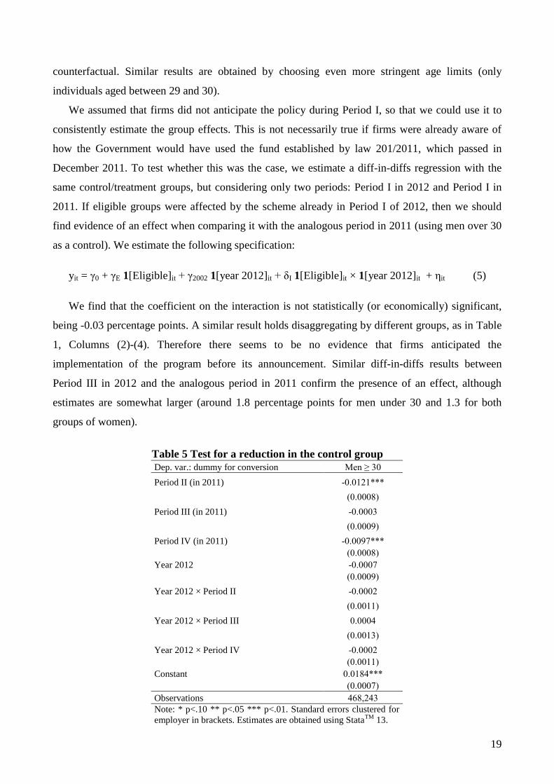
We assumed that firms did not anticipate the policy during Period I, so that we could use it to

consistently estimate the group effects. This is not necessarily true if firms were already aware of

how the Government would have used the fund established by law 201/2011, which passed in

December 2011. To test whether this was the case, we estimate a diff-in-diffs regression with the

same control/treatment groups, but considering only two periods: Period I in 2012 and Period I in

2011. If eligible groups were affected by the scheme already in Period I of 2012, then we should

find evidence of an effect when comparing it with the analogous period in 2011 (using men over 30

as a control). We estimate the following specification:

yit = γ0 + γE 1[Eligible]it + γ2002 1[year 2012]it + δI 1[Eligible]it × 1[year 2012]it + ηit (5)

We find that the coefficient on the interaction is not statistically (or economically) significant,

being -0.03 percentage points. A similar result holds disaggregating by different groups, as in Table

1, Columns (2)-(4). Therefore there seems to be no evidence that firms anticipated the

implementation of the program before its announcement. Similar diff-in-diffs results between

Period III in 2012 and the analogous period in 2011 confirm the presence of an effect, although

estimates are somewhat larger (around 1.8 percentage points for men under 30 and 1.3 for both

groups of women).

Table 5 Test for a reduction in the control group

Dep. var.: dummy for conversion Men ≥ 30

Period II (in 2011) -0.0121***

(0.0008)

Period III (in 2011) -0.0003

(0.0009)

Period IV (in 2011) -0.0097***

(0.0008)

Year 2012 -0.0007

(0.0009)

Year 2012 × Period II -0.0002

(0.0011)

Year 2012 × Period III 0.0004

(0.0013)

Year 2012 × Period IV -0.0002

(0.0011)

Constant 0.0184***

(0.0007)

Observations 468,243

Note: * p<.10 ** p<.05 *** p<.01. Standard errors clustered for

employer in brackets. Estimates are obtained using StataTM

13.

20

Besides anticipation/delay effects, which refer to the eligible groups, employers could have also

substituted conversions for the control group in favor of those for the eligible workers. If this

happened, we would expect to find the trend over the four periods for the control group to show a

dip in Period III. Given that a similar dip could have been present also in 2011, we test whether the

trend over periods I to IV was different in 2012 with respect to 2011. Results are reported in Table

5. A test for the interactions between the dummy for 2012 and the dummies for periods II-III-IV

being jointly equal to zero fails to reject the null with p-value 0.9381. Therefore the evidence is not

against the assumption that the control group has been (on average) unaffected by the policy.

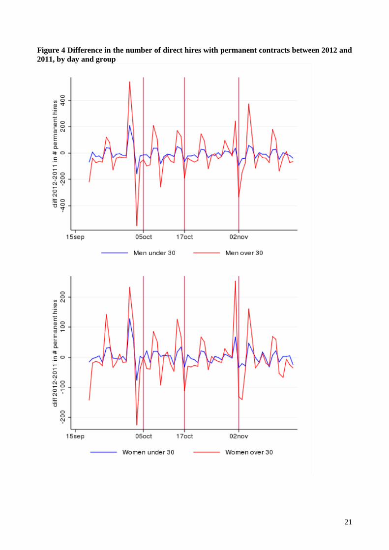
Another possible substitution could take place between conversions (from fixed-term to

permanent positions) and direct hires with a permanent contract. In Figure 4 we show the time

series of the daily difference between the number of direct hires with a permanent contract in 2012

and in 2011, for different groups. There is no evidence of a change in the number of direct hiring

during the period of validity of the policy.

Additional robustness tests have also been implemented. For instance, a possible difficulty is

related with the circumstance that, for bureaucratic reasons, conversions are more likely at the turn

of a month. In our case, however, the effect is not driven by conversions taking place at the end of

October or begin of November: excluding the days in [30/10-02/11] we still find evidence of an

impact for the eligible group. In terms of possible anticipation effects, we also worried that

countervailing effects on the conversion rates of eligible workers can be found later than Period IV,

which does not include the begin of a month. To check for this possibility, we added two

subsequent periods of 16-day length, plugging therefore dates until December the 19th

, and checked

whether negative effects were in place. The results are reassuring. There is only a weak evidence of

some small decrease for women aged less than 30 in period [04/12-19/12], with an estimate -0.26

percentage points marginally significant at the 5% level (p-value 0.050), but which is actually

similar to the coefficient we found in a falsification on 2011 (-0.17 percentage points, p-value

0.243). Finally, the incentives for conversions could be cumulated with others available for hiring

workers that have been previously dismissed through a particular procedure, called mobilità. We

also replicated all our regressions by excluding these employees, again with no significant changes

in the findings.

21

Figure 4 Difference in the number of direct hires with permanent contracts between 2012 and

2011, by day and group

22

6.3 Heterogeneity

The results documented so far for the groups of eligible workers might mask relevant

heterogeneities. An important issue refers to the impact of the scheme across skill groups. For

instance, a policy maker might want to know whether the program works for those who are less

endowed with human capital, as their performance in the labor market is usually more problematic.

In the following, for simplicity, we only focus on the effects that materialize in Period III.

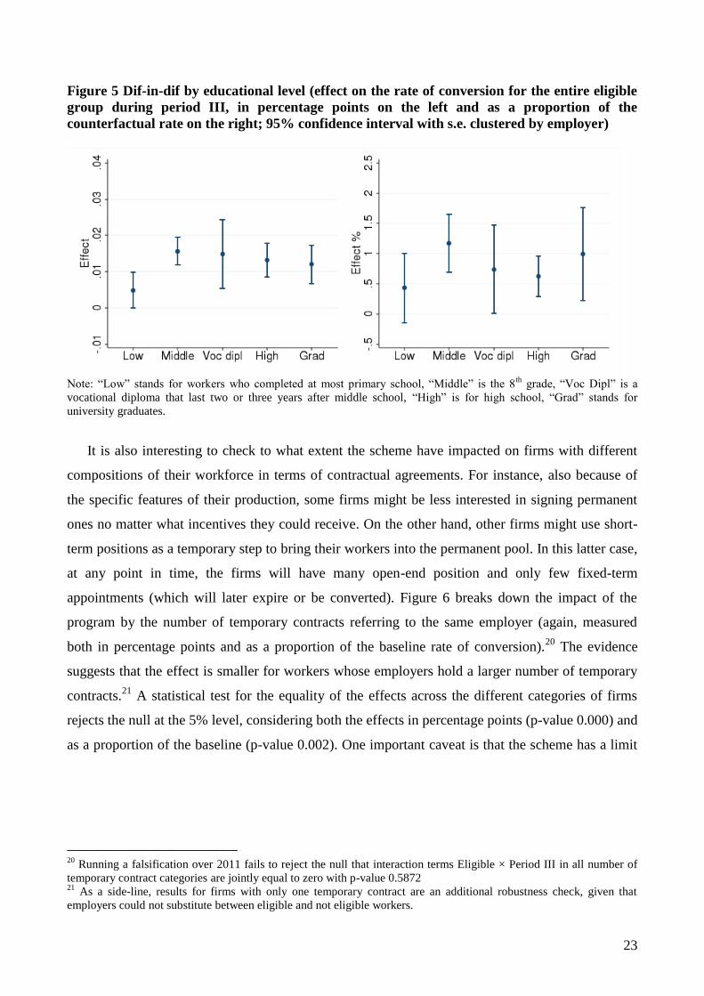
Figure 5 shows, for the eligible groups taken as a whole, the breakdown by educational level of

the estimated effect (measured in percentage points, on the left, and as a proportion of the

counterfactual rate, on the right).17

The impact of the scheme seems to be lower for those who have

at most completed primary school. However, this is a relatively small group, accounting for only

10.7% of the observations for eligible workers in 2012. Differently, starting from middle school (8th

grade) there is no evidence of strong heterogeneity: most of the effects are positive and there is no

systematic increase associated with higher qualifications. Furthermore, the effects are all

significantly different from zero at the 5% level. Similar conclusions can be taken by looking at the

proportional effect, although it must be considered that these estimates are less precise due to the

fact that even the baseline rate of conversion is estimated through the same model. Results obtained

by breaking down the educational levels for each single group (young men, young women and older

females) of eligible workers are qualitatively similar (and available on request). One potential

concern is that the reduction in the number of observations, and in particular in the total number of

observed conversions, for each cell of group × period × educational qualification makes estimates

largely imprecise, hindering the ability to detect heterogeneity. To lessen this concern, we also

estimated the average effects using only low qualifications (middle school or less) on the one hand,

and high qualifications (high school or above) on the other.18

Results are only marginally modified:

the 95% confidence interval for the effect in percentage point is [.0098; .0161] for low

qualifications, which is very similar to that estimated for the other group, [.0089; .0163].19

Overall,

it seems safe to conclude that the impact of the scheme was quite homogeneous across skill groups.

17

The information on the educational qualification is reported by the employer at the moment of the communication to

the regional agency. There are 0,7% of the observations with a missing values. Given that for foreign citizen this

information is likely to contain measurement error, we also reproduced the graph keeping only Italian citizen, but we

found no qualitative differences. It must also be added that the falsification over 2011 fails to reject the null that

interaction terms Eligible × Period III in all educational group are jointly equal to zero with p-value 0.1461. 18

We did not consider vocational diploma, which are a particular case in between low and high qualification.

Nevertheless, they involve only around 5.5% of the eligible observations, and the effect for them is similar to the one

for high school graduates. 19

Given that the baseline rate of conversions is higher for the most educated, these results imply a smaller percentage

increase for them, although we always fail to reject the null that the proportional effect is different (with high p-values).

23

Figure 5 Dif-in-dif by educational level (effect on the rate of conversion for the entire eligible

group during period III, in percentage points on the left and as a proportion of the

counterfactual rate on the right; 95% confidence interval with s.e. clustered by employer)

Note: “Low” stands for workers who completed at most primary school, “Middle” is the 8

th grade, “Voc Dipl” is a

vocational diploma that last two or three years after middle school, “High” is for high school, “Grad” stands for

university graduates.

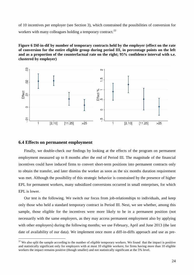
It is also interesting to check to what extent the scheme have impacted on firms with different

compositions of their workforce in terms of contractual agreements. For instance, also because of

the specific features of their production, some firms might be less interested in signing permanent

ones no matter what incentives they could receive. On the other hand, other firms might use short-

term positions as a temporary step to bring their workers into the permanent pool. In this latter case,

at any point in time, the firms will have many open-end position and only few fixed-term

appointments (which will later expire or be converted). Figure 6 breaks down the impact of the

program by the number of temporary contracts referring to the same employer (again, measured

both in percentage points and as a proportion of the baseline rate of conversion).20

The evidence

suggests that the effect is smaller for workers whose employers hold a larger number of temporary

contracts.21

A statistical test for the equality of the effects across the different categories of firms

rejects the null at the 5% level, considering both the effects in percentage points (p-value 0.000) and

as a proportion of the baseline (p-value 0.002). One important caveat is that the scheme has a limit

20

Running a falsification over 2011 fails to reject the null that interaction terms Eligible × Period III in all number of

temporary contract categories are jointly equal to zero with p-value 0.5872 21

As a side-line, results for firms with only one temporary contract are an additional robustness check, given that

employers could not substitute between eligible and not eligible workers.

24

of 10 incentives per employer (see Section 3), which constrained the possibilities of conversion for

workers with many colleagues holding a temporary contract.22

Figure 6 Dif-in-dif by number of temporary contracts held by the employer (effect on the rate

of conversion for the entire eligible group during period III, in percentage points on the left

and as a proportion of the counterfactual rate on the right; 95% confidence interval with s.e.

clustered by employer)

6.4 Effects on permanent employment

Finally, we double-check our findings by looking at the effects of the program on permanent

employment measured up to 8 months after the end of Period III. The magnitude of the financial

incentives could have induced firms to convert short-term positions into permanent contracts only

to obtain the transfer, and later dismiss the worker as soon as the six months duration requirement

was met. Although the possibility of this strategic behavior is constrained by the presence of higher

EPL for permanent workers, many subsidized conversions occurred in small enterprises, for which

EPL is lower.

Our test is the following. We switch our focus from job-relationships to individuals, and keep

only those who held a standard temporary contract in Period III. Next, we see whether, among this

sample, those eligible for the incentives were more likely to be in a permanent position (not

necessarily with the same employers, as they may access permanent employment also by applying

with other employers) during the following months; we use February, April and June 2013 (the last

date of availability of our data). We implement once more a diff-in-diffs approach and use as pre-

22

We also split the sample according to the number of eligible temporary workers. We found that the impact is positive

and statistically significant only for employers with at most 10 eligible workers; for firms having more than 10 eligible

workers the impact remains positive (though smaller) and not statistically significant at the 5% level.

25

policy counterfactuals the individuals who held temporary contracts in the 2011 period analogous to

Period III, for which their employment status is measured during the first semester of 2012.

Formally, we estimate a diff-in-diffs regression of the type:

yit = λ0 + λE 1[Eligible]it + λ 2002 1[year 2012]it + θ 1[Eligible]it × 1[year 2012]it + μit (6)

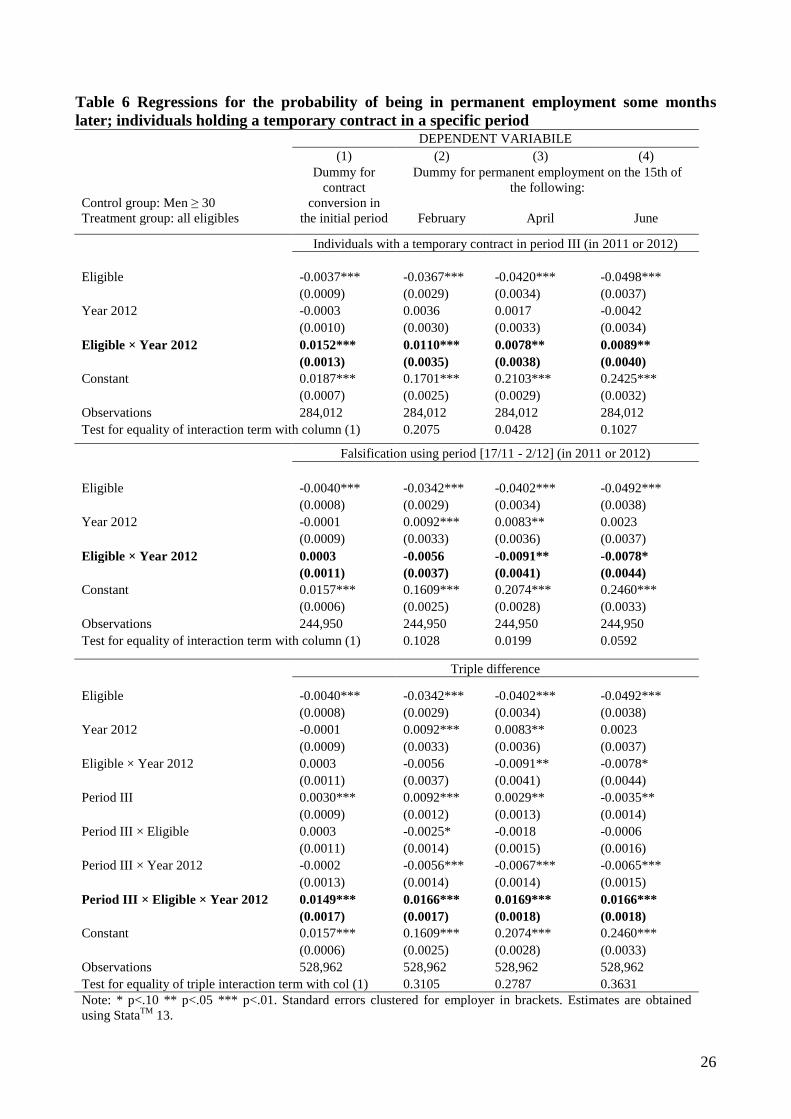
Table 6 describes the results. In the first panel, Column (1) describes the estimates of the

probability of conversion during Period III. Columns (2), (3) and (4) provides the estimates of the

chance of being in permanent employment in the following months. Our evidence suggests a

significant increase in the probability of conversion (at the individual level) in Period III (the

magnitude of the effect is larger, but compatible with the results where the unit of observation is the

job-relationship). We also find positive and statistically effects as for the likelihood of being

permanent in February, April and June 2013. Note that the point estimates for the impact on

permanent employment later in time are smaller than the increase in conversion probability in

Period III. Although the difference is statistically significant at the 5% level only in one case

(April), this finding could signal that a fraction of the subsidized conversions went to individuals

who would have accessed permanent employment even in the absence of the incentives.

However, we have to make sure that the eligible group does not show a diverging trend in the

probability of accessing permanent employment during the first semester of 2013. In the second

panel of Table 6, we run a falsification exercise, by focusing on individuals holding a temporary

contract in the following month, between 17/11 and 2/12. As we have already discussed, in this

period incentives were not available anymore. According to our evidence of no substitution over

time we expect these individuals to be unaffected by the policy. Indeed, column (1) of the second

panel in Table 6 shows that there is no effect on the conversion rate of eligible individuals in this

period. We can therefore use this group to infer whether eligible workers would have shown a

diverging trend in the absence of the incentives. If there is evidence of a downward trend (with

respect to men over 30) in the probability of getting a permanent job, we would be underestimating

the effects of the incentives. In columns (2)-(4), second panel, we find that the probability of being

in permanent employment later in time (in April and June) decreases by around 0.8-0.9 percentage

points for eligible workers. Note that this gap is similar to the difference between the effect on

conversion and that on permanent employment documented in the first panel.

26

Table 6 Regressions for the probability of being in permanent employment some months

later; individuals holding a temporary contract in a specific period DEPENDENT VARIABILE

(1) (2) (3) (4)

Control group: Men ≥ 30

Treatment group: all eligibles

Dummy for

contract

conversion in

the initial period

Dummy for permanent employment on the 15th of

the following:

February April June

Individuals with a temporary contract in period III (in 2011 or 2012)

Eligible -0.0037*** -0.0367*** -0.0420*** -0.0498***

(0.0009) (0.0029) (0.0034) (0.0037)

Year 2012 -0.0003 0.0036 0.0017 -0.0042

(0.0010) (0.0030) (0.0033) (0.0034)

Eligible × Year 2012 0.0152*** 0.0110*** 0.0078** 0.0089**

(0.0013) (0.0035) (0.0038) (0.0040)

Constant 0.0187*** 0.1701*** 0.2103*** 0.2425***

(0.0007) (0.0025) (0.0029) (0.0032)

Observations 284,012 284,012 284,012 284,012

Test for equality of interaction term with column (1) 0.2075 0.0428 0.1027

Falsification using period [17/11 - 2/12] (in 2011 or 2012)

Eligible -0.0040*** -0.0342*** -0.0402*** -0.0492***

(0.0008) (0.0029) (0.0034) (0.0038)

Year 2012 -0.0001 0.0092*** 0.0083** 0.0023

(0.0009) (0.0033) (0.0036) (0.0037)

Eligible × Year 2012 0.0003 -0.0056 -0.0091** -0.0078*

(0.0011) (0.0037) (0.0041) (0.0044)

Constant 0.0157*** 0.1609*** 0.2074*** 0.2460***

(0.0006) (0.0025) (0.0028) (0.0033)

Observations 244,950 244,950 244,950 244,950

Test for equality of interaction term with column (1) 0.1028 0.0199 0.0592

Triple difference

Eligible -0.0040*** -0.0342*** -0.0402*** -0.0492***

(0.0008) (0.0029) (0.0034) (0.0038)

Year 2012 -0.0001 0.0092*** 0.0083** 0.0023

(0.0009) (0.0033) (0.0036) (0.0037)

Eligible × Year 2012 0.0003 -0.0056 -0.0091** -0.0078*

(0.0011) (0.0037) (0.0041) (0.0044)

Period III 0.0030*** 0.0092*** 0.0029** -0.0035**

(0.0009) (0.0012) (0.0013) (0.0014)

Period III × Eligible 0.0003 -0.0025* -0.0018 -0.0006

(0.0011) (0.0014) (0.0015) (0.0016)

Period III × Year 2012 -0.0002 -0.0056*** -0.0067*** -0.0065***

(0.0013) (0.0014) (0.0014) (0.0015)

Period III × Eligible × Year 2012 0.0149*** 0.0166*** 0.0169*** 0.0166***

(0.0017) (0.0017) (0.0018) (0.0018)

Constant 0.0157*** 0.1609*** 0.2074*** 0.2460***

(0.0006) (0.0025) (0.0028) (0.0033)

Observations 528,962 528,962 528,962 528,962

Test for equality of triple interaction term with col (1) 0.3105 0.2787 0.3631

Note: * p<.10 ** p<.05 *** p<.01. Standard errors clustered for employer in brackets. Estimates are obtained

using StataTM

13.

27

Therefore, we find evidence of a diverging negative trend for the eligible group. In order to

correct for it, the third panel runs a triple difference regression, which is simply equivalent of

subtracting panel 2 from panel 1. The effect of the policy is now captured by the coefficient on the

triple difference Period III × Eligible × Year 2012. The point estimates for employment are now

quite stable over time and comparable with the conversion rate, although slightly larger.

We also did an additional check. We replicated the second and third panel of Table 6 by removing,

from the group of individuals holding a fixed-term contract between 17/11 and 2/12, those hired by

firms who had previously done a conversion in period III. This should minimize the risk of

substitution over time and across workers, because it excludes those employers who could have

anticipated strategically conversions during period III. Results, available on request, are in line with

those presented here.

All in all, our findings suggest that – when measured 8 months after the scheme was over – the

impact on permanent employment is still there. More in general, it shows that those individuals who

benefited from the increased conversion rate would not have found a permanent job in the absence

of the policy. Nevertheless, part of the stability of the effect over time may be due to the fact that

the incentives were distributed only under the condition that the contract lasted at least six months

after the conversion.

7. Conclusions

Our exercise suggests that the program introduced with the Decree 5 Oct 2012 was effective in

stimulating conversions. Compared to the counterfactual scenario, conversions increased by 83%.

The additional permanent positions came with a cost: to get one extra-permanent job the

government had to finance additional 1.2 conversions that would have taken place even with no

public support.

No need to say, the external validity of program evaluation experiments is quite low. Thus, it is

not safe to infer from our results policy implications of general validity as for the effectiveness of

conversion programs. Having said so, a number of remarks are in order.

First, the scheme we evaluated shows little sign of perverse conducts on the employer side

There is no evidence of strategic behavior, intended to bring conversions forward or backward only

to benefit from the scheme. This circumstance might well be explained by the fact that the span of

time between announcement and beginning of the program was small and the shortage of financing

might have come before than excepted (by the employers).

Secondly, it is very difficult to say whether the amount of the subsidy was appropriate to the aim

of converting the maximum amount possible of short-term positions. A higher financial support

28

could have spurred additional conversions; at the same time, it would have made even larger the

financial dead-weight loss associated with the conversions that would have been done even without

the scheme. Therefore, within the budget constraint envisaged by Decree 5 Oct 2012, increasing the

subsidy might not necessarily help with converting more contracts. If one believes that employers’

demand for conversions was fully fulfilled at that amount of the subsidy, then it is not unrealistic

that a smaller amount of money would have reached a similar effectiveness.

Finally, it might be useful to compare the program with two different schemes of incentives

aimed at promoting permanent employment, which were introduced in Italy at different points in

time. In year 2000, Law 388 established a tax-credit (of 413 euro per month; 620 in the South of

Italy) for each unit increase in the number of permanent workers aged 25 or more with respect to

the figure reported by the firm for the pre-policy year. The scheme also required the employers to

increase the overall workforce. Essentially, employers could access the incentive by hiring a new

worker with a permanent contract, or by converting a fixed-term one but simultaneously hiring a

new temporary (or permanent) worker. For this scheme, Cipollone and Guelfi (2006) find no sign of

overall effectiveness, as for the probability that individuals enter into permanent employment.

However, they find a positive effect for those previously employed with a temporary training

contract, suggesting that these incentives may be more likely to have an impact on conversions

rather than on new hires. Their estimates were also positive for the unemployed with previous work

experience and for more educated workers, while basically zero for those without a high school

diploma.

A more recent measure was introduced by a law-decree in June 2013 (the so called “decreto

lavoro”), which aimed at improving employability of young individuals within the framework of

the Youth Guarantee. Starting from August 2013, employers who hired with permanent contracts

individuals aged 18-29, either unemployed for at least 6 months or without a high school or

vocational diploma, could receive an incentive of 1/3 of the gross salary (with a cap at 650 euro) for

18 months. The same applied for conversions from fixed term to permanent contracts, although the

duration of the subsidy was limited to 12 months. In both cases, the employer had to increase

his/her overall workforce, similarly to the 2001 policy. As reported by the Ministry of Labor on the

18th

of December 2013 the number of applications for this scheme was around 18,000, a relatively

small number with respect to the potential amount of incentives allowed by the available funding

(around 100,000).

One important difference between these two programs and the one we studied is that they the

required the employer to increase the workforce. This might be an important reason why the Decree

5 October 2012 seems to have had a larger impact. Clearly, whether a policy maker should or not

29

impose this additional constraint also depends on the final target of the scheme, which may aim at

increasing overall employment and not only the rate of conversion.

Another important difference is that the Decree 5 October 2012 did not finance direct hires with

a permanent contract, but only conversions. As argued by Cipollone and Guelfi (2003, 2006), their

finding of heterogeneous effects of law 388/2000 can be explained by the fact that employers

prefers to hire permanently only individuals with a stronger signal of higher productivity, in

particular the more educated and those with previous work experience. Differently from them we

find an aggregate positive effect and no significant differences according to the educational level of

the worker. This suggests that the incentives for conversions may be more effective, generating less

dead-weight loss, because they exploit the stepping-stone effect of fixed-term contracts.

References

Anastasia, B., Disarò, M., Gambuzza, M., Rasera M., 2009, Comunicazioni obbligatorie e

analisi congiunturale del mercato del lavoro: evoluzione, problemi metodologici, risultati, collana “I

tartufi” n. 35, Veneto Lavoro.

Anastasia, B., Disarò, M., Emireni, G., Gambuzza, M., Rasera, M., 2010, Guida all'uso delle

Comunicazioni Obbligatorie nel monitoraggio del mercato del lavoro. Seconda versione: dicembre

2010, collana “I tartufi” n. 36, Veneto Lavoro.

Anastasia, B., Giraldo, A., Paggiaro, A., 2013. L’effetto degli incentivi alle assunzioni e alle

trasformazioni. Prime evidenze per il Veneto. Politica Economica, a. XXIX, n.2, 181-198.

Angrist, J.D., Pischke, J.S., 2009. Mostly Harmless Econometrics. Princeton University Press.

Arulampalam, W., Booth, A.L. 1998. Training and Labour Market Flexibility: Is There a Trade-

off? British Journal of Industrial Relations 36(4), 521-536.

Arulampalam, W., Booth, A.L., Bryan, M.L. 2004. Training in Europe. Journal of the European

Economic Association 2(2-3), 346-360.

Barbieri, G., Sestito, P., 2008. Temporary Workers in Italy: Who Are They and Where They

End Up? LABOUR 22, 127–166.

Battiloro, V., Mo Costabella, L., 2011. Incentivi o misure di attivazione? Evidenze sull’efficacia

di due interventi per contrastare il lavoro precario, Politica Economica, a. XXVII, n.2., 197-218.

Becker, S. O., Bentolila, S., Fernandes, A., Ichino, A. 2010. Youth emancipation and perceived

job insecurity of parents and children. Journal of Population Economics 23, 1175-1199.

30

Bertola, G., 1990. Job security, employment and wages. European Economic Review 34, 851-

879.

Berton, F., Devicienti, F., Pacelli, L., 2011. Are temporary jobs a port of entry into permanent

employment? Evidence from matched employer-employee data. International Journal of Manpower

32, 879–899.

Blundell, R., MaCurdy, T., 1999. Labor supply: A review of alternative approaches. in

Handbook of Labor Economics, edited by O. Ashenfelter & D. Card, edition 1, volume 3, chapter

27, 1559-1695.

Blundell, R., Francesconi, M., van der Klaauw, W. 2011. Anatomy of Welfare Reforms:

Announcement and Implementation Effects, IZA Discussion Papers No. 6050, Institute for the

Study of Labor.

Boeri, T., Jimeno, J., 2005. The effects of employment protection: learning from variable

enforcement. European Economic Review 49, 2057–2077.

Booth, A.L., Francesconi, M., Frank, J., 2002. Temporary Jobs: Stepping Stones or Dead Ends?

The Economic Journal 112, F189–F213.

Bruno, G. S. F., Caroleo, F. E., Dessy, O. 2012. Stepping Stones versus Dead End Jobs: Exits

from Temporary Contracts in Italy after the 2003 Reform, IZA Discussion Paper No. 6746, Institute

for the Study of Labor.

Cappellari, L., Dell’Aringa, C., Leonardi, M., 2012. Temporary Employment, Job Flows and

Productivity: a Tale of Two Reforms. The Economic Journal 122, F188–F215.

Cipollone, P., Guelfi, A., 2003. Tax credit policy and firms’ behaviour: the case of subsidies to

open-end contracts in Italy. Temi di Discussione No. 471, Bank of Italy.

Cipollone, P., Guelfi, A., 2006. Financial support to permanent jobs. The Italian case. Politica

Economica a. XXII, n. 1, 51–75.

Engellandt, A., Riphahn, R. T. 2005. Temporary contracts and employee effort. Labour

Economics 12, 281-299.

Grassi, E., 2009. The effect of EPL on the conversion rate of temporary contracts into

permanent contracts: Evidence from Italy. Giornale degli Economisti 68, 211–231.

Hernanz, V., Jimeno, J.F., Kugler, A.D., 2003. Employment consequences of restrictive

permanent contracts: Evidence from Spanish labour market reforms. CEPR Discussion Papers 3724

31

Ichino, A., Mealli, F., Nannicini, T., 2005. Temporary Work Agencies in Italy: A Springboard

Toward Permanent Employment? Giornale degli Economisti 64, 1–27.

Kugler, A., Pica, G., 2008. Effects of employment protection on worker and job flows: Evidence

from the 1990 Italian reform. Labour Economics 15, 78–95.

Maurin, E., Michaud, M.. 2004. The Effects of Increasing the Costs of Fixed-Term Contracts on

the Dynamics of Labor Demand: An Evaluation of a French Reform, paper presented at the

CEPR/ECB Labour Market Conference, available at

http://dev3.cepr.org/meets/wkcn/4/4539/papers/maurin.pdf

Maurizio, D., 2006. Giove: un database statistico sul mercato del lavoro veneto, collana “I

tartufi” n. 22, Veneto Lavoro.

Méndez, I., 2013. Promoting Permanent Employment: Lessons from Spain. Journal of the

Spanish Economic Association 4, 175–199.

Modena, F., Sabatini, F., 2012. I would if I could: precarious employment and childbearing

intentions in Italy. Review of the Economics of the Household 10, 77-97.

Picchio, M., 2008. Temporary Contracts and Transitions to Stable Jobs in Italy. LABOUR 22,

147–174.

Priftin, E., Vuri, D., 2013. Employment protection and fertility: evidence from the 1990 Italian

reform. Labour Economics 23, 77-88.

Schivardi, F., Torrini, R., 2008. Identifying the effects of firing restrictions through size-

contingent differences in regulation. Labour Economics 15, 482–511.

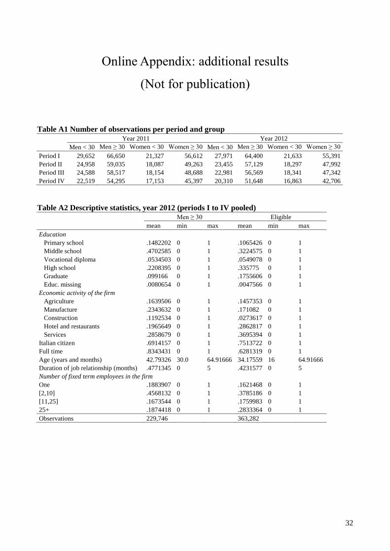
32

Online Appendix: additional results

(Not for publication)

Table A1 Number of observations per period and group

Year 2011 Year 2012

Men < 30 Men ≥ 30 Women < 30 Women ≥ 30 Men < 30 Men ≥ 30 Women < 30 Women ≥ 30

Period I 29,652 66,650 21,327 56,612 27,971 64,400 21,633 55,391

Period II 24,958 59,035 18,087 49,263 23,455 57,129 18,297 47,992

Period III 24,588 58,517 18,154 48,688 22,981 56,569 18,341 47,342

Period IV 22,519 54,295 17,153 45,397 20,310 51,648 16,863 42,706

Table A2 Descriptive statistics, year 2012 (periods I to IV pooled)

Men ≥ 30 Eligible

mean min max mean min max

Education

Primary school .1482202 0 1 .1065426 0 1

Middle school .4702585 0 1 .3224575 0 1

Vocational diploma .0534503 0 1 .0549078 0 1

High school .2208395 0 1 .335775 0 1

Graduate .099166 0 1 .1755606 0 1

Educ. missing .0080654 0 1 .0047566 0 1

Economic activity of the firm

Agriculture .1639506 0 1 .1457353 0 1

Manufacture .2343632 0 1 .171082 0 1

Construction .1192534 0 1 .0273617 0 1

Hotel and restaurants .1965649 0 1 .2862817 0 1

Services .2858679 0 1 .3695394 0 1

Italian citizen .6914157 0 1 .7513722 0 1

Full time .8343431 0 1 .6281319 0 1

Age (years and months) 42.79326 30.0 64.91666 34.17559 16 64.91666

Duration of job relationship (months) .4771345 0 5 .4231577 0 5

Number of fixed term employees in the firm

One .1883907 0 1 .1621468 0 1

[2,10] .4568132 0 1 .3785186 0 1

[11,25] .1673544 0 1 .1759983 0 1

25+ .1874418 0 1 .2833364 0 1

Observations 229,746 363,282

33

Table A3 Additional robustness checks (probability of conversion from temporary to

permanent contract during each single period in 2012)

(1) (2) (3) (4) (5)

Control group: Men ≥ 30

Treatment group: all eligibles

Dependent variable: dummy

for conversion

Including all

temporary

contracts

Excluding

those in the

economic

sectors of

Public

Administration

Education and

Health

Excluding

those with a

Public

Administration

national

contract

Excluding

those with

contract

duration larger

than 3 years

Age defined at

the end of the

period

Eligible -0.0029*** -0.0018** -0.0015* -0.0023*** -0.0021***

(0.0006) (0.0008) (0.0008) (0.0007) (0.0007)

Period II -0.0109*** -0.0127*** -0.0128*** -0.0123*** -0.0123***

(0.0007) (0.0008) (0.0008) (0.0007) (0.0007)

Period III -0.0001 0.0004 0.0003 0.0001 0.0003

(0.0008) (0.0010) (0.0010) (0.0009) (0.0009)

Period IV -0.0090*** -0.0101*** -0.0102*** -0.0099*** -0.0099***

(0.0007) (0.0008) (0.0008) (0.0008) (0.0008)

Eligible × Period II 0.0018*** 0.0011 0.0007 0.0013 0.0011

(0.0007) (0.0009) (0.0009) (0.0008) (0.0008)

Eligible × Period III 0.0098*** 0.0144*** 0.0147*** 0.0132*** 0.0128***

(0.0010) (0.0014) (0.0013) (0.0012) (0.0012)

Eligible × Period IV 0.0023*** 0.0022** 0.0019** 0.0021** 0.0020**

(0.0007) (0.0010) (0.0010) (0.0009) (0.0009)

Constant 0.0155*** 0.0184*** 0.0183*** 0.0177*** 0.0177***

(0.0007) (0.0007) (0.0007) (0.0007) (0.0007)

Observations 778,568 519,196 550,489 589,490 592,967

Effect / counterfactual (period

III) 0.7813 0.8445 0.8616 0.8530 0.8084

Note: * p<.10 ** p<.05 *** p<.01. Standard errors clustered for employer in brackets. Estimates are obtained using

StataTM

13. See Figure 1 for the definition of periods.

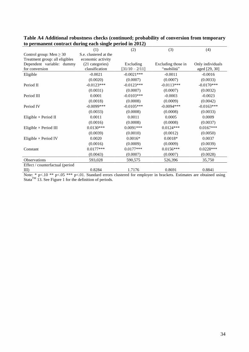
34

Table A4 Additional robustness checks (continued; probability of conversion from temporary

to permanent contract during each single period in 2012)

(1) (2) (3) (4)

Control group: Men ≥ 30

Treatment group: all eligibles

Dependent variable: dummy

for conversion

S.e. clustered at the

economic activity

(21 categories)

classification

Excluding

[31/10 – 2/11]

Excluding those in

“mobilità”

Only individuals

aged [29, 30]

Eligible -0.0021 -0.0021*** -0.0011 -0.0016

(0.0020) (0.0007) (0.0007) (0.0033)

Period II -0.0123*** -0.0123*** -0.0113*** -0.0170***

(0.0031) (0.0007) (0.0007) (0.0032)

Period III 0.0001 -0.0103*** -0.0003 -0.0023

(0.0018) (0.0008) (0.0009) (0.0042)

Period IV -0.0099*** -0.0105*** -0.0094*** -0.0163***

(0.0033) (0.0008) (0.0008) (0.0033)

Eligible × Period II 0.0011 0.0011 0.0005 0.0009

(0.0016) (0.0008) (0.0008) (0.0037)

Eligible × Period III 0.0130*** 0.0091*** 0.0124*** 0.0167***

(0.0039) (0.0010) (0.0012) (0.0050)

Eligible × Period IV 0.0020 0.0016* 0.0018* 0.0037

(0.0016) (0.0009) (0.0009) (0.0039)

Constant 0.0177*** 0.0177*** 0.0156*** 0.0228***

(0.0043) (0.0007) (0.0007) (0.0028)

Observations 593,028 590,575 526,396 35,750

Effect / counterfactual (period

III) 0.8284 1.7176 0.8691 0.8841

Note: * p<.10 ** p<.05 *** p<.01. Standard errors clustered for employer in brackets. Estimates are obtained using

StataTM

13. See Figure 1 for the definition of periods.

35

Table A5 Replication of Table 6, but removing from the falsification those firms who

converted a contract during period III DEPENDENT VARIABLE

(1) (2) (3) (4)

Control group: Men ≥ 30

Treatment group: all eligibles

Dummy for

contract

conversion in

the initial period

Dummy for permanent employment on the 15th of

the following:

February April June

Falsification using period [17/11 - 2/12] (in 2011 or 2012)

Eligible -0.0039*** -0.0352*** -0.0416*** -0.0519***

(0.0008) (0.0029) (0.0035) (0.0038)

Year 2012 -0.0005 0.0112*** 0.0098** 0.0024

(0.0009) (0.0037) (0.0041) (0.0043)

Eligible × Year 2012 0.0009 -0.0064 -0.0096** -0.0067

(0.0011) (0.0039) (0.0042) (0.0044)

Constant 0.0145*** 0.1561*** 0.2012*** 0.2394***

(0.0006) (0.0023) (0.0026) (0.0029)

Observations 218,034 218,034 218,034 218,034

Test for equality of interaction term with column (1) 0.0542 0.0118 0.0803

Triple difference

Eligible -0.0039*** -0.0352*** -0.0416*** -0.0519***

(0.0008) (0.0029) (0.0035) (0.0038)

Year 2012 -0.0005 0.0112*** 0.0098** 0.0024

(0.0009) (0.0037) (0.0041) (0.0043)

Eligible × Year 2012 0.0009 -0.0064 -0.0096** -0.0067

(0.0011) (0.0039) (0.0042) (0.0044)

Period III 0.0042*** 0.0140*** 0.0092*** 0.0031

(0.0009) (0.0017) (0.0019) (0.0021)

Period III × Eligible 0.0002 -0.0016 -0.0004 0.0021

(0.0011) (0.0019) (0.0021) (0.0022)

Period III × Year 2012 0.0002 -0.0076*** -0.0082*** -0.0066**

(0.0013) (0.0022) (0.0025) (0.0028)

Period III × Eligible × Year 2012 0.0143*** 0.0174*** 0.0173*** 0.0156***

(0.0017) (0.0024) (0.0026) (0.0028)

Constant 0.0145*** 0.1561*** 0.2012*** 0.2394***

(0.0006) (0.0023) (0.0026) (0.0029)

Observations 502,046 502,046 502,046 502,046

Test for equality of triple interaction term with col (1) 0.1761 0.2253 0.6516

Note: * p<.10 ** p<.05 *** p<.01. Standard errors clustered for employer in brackets. Estimates are obtained

using StataTM

13.