Get Wet: Creek Flow

Noah Granigan

September 27, 2018

MCEN 4151-001: Flow Visualization

University of Colorado Boulder

Get Wet: Creek Flow

Noah Granigan

2

I. INTRODUCTION

The aptly named Get Wet assignment gave me the goal to get my feet wet in flow visualization.

The intent of the image was to demonstrate the different areas of turbulent flow downstream of a

rock in Boulder Creek. I tried many different camera angles with this rock, including a birds-eye,

upstream, and downstream view. The upstream view, displayed in Figure 1 had the best view for

being able to tell what was going on in the creek. The moving water creates a space with an absence

of downstream-flow, and water flows into the void creating a swirl of water on each edge of the

obstacle. Although it was unable to be captured in my image, flow can travel upstream to fill this

void.[1]

II. APPARATUS & FLUID MECHANICS

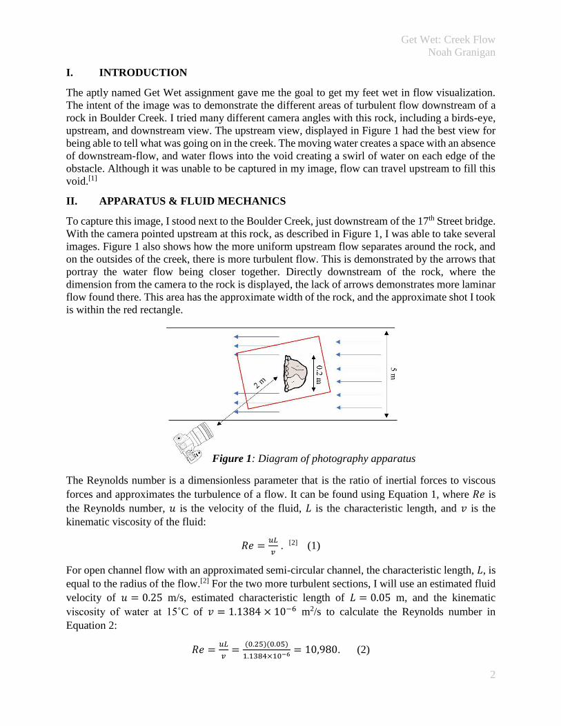
To capture this image, I stood next to the Boulder Creek, just downstream of the 17th Street bridge.

With the camera pointed upstream at this rock, as described in Figure 1, I was able to take several

images. Figure 1 also shows how the more uniform upstream flow separates around the rock, and

on the outsides of the creek, there is more turbulent flow. This is demonstrated by the arrows that

portray the water flow being closer together. Directly downstream of the rock, where the

dimension from the camera to the rock is displayed, the lack of arrows demonstrates more laminar

flow found there. This area has the approximate width of the rock, and the approximate shot I took

is within the red rectangle.

Figure 1: Diagram of photography apparatus

The Reynolds number is a dimensionless parameter that is the ratio of inertial forces to viscous

forces and approximates the turbulence of a flow. It can be found using Equation 1, where 𝑅𝑒 is

the Reynolds number, 𝑢 is the velocity of the fluid, 𝐿 is the characteristic length, and 𝑣 is the

kinematic viscosity of the fluid:

𝑅𝑒 =𝑢𝐿

𝑣 . [2] (1)

For open channel flow with an approximated semi-circular channel, the characteristic length, 𝐿, is

equal to the radius of the flow.[2] For the two more turbulent sections, I will use an estimated fluid

velocity of 𝑢 = 0.25 m/s, estimated characteristic length of 𝐿 = 0.05 m, and the kinematic

viscosity of water at 15˚C of 𝑣 = 1.1384 × 10−6 m2/s to calculate the Reynolds number in

Equation 2:

𝑅𝑒 =𝑢𝐿

𝑣=

(0.25)(0.05)

1.1384×10−6= 10,980. (2)

Get Wet: Creek Flow

Noah Granigan

3

For the less turbulent section directly downstream of the rock, I will use an estimated fluid velocity

of 𝑢 = 0.05 m/s, estimated characteristic length of 𝐿 = 0.1 m, and the kinematic viscosity of water

at 15˚C of 𝑣 = 1.1384 × 10−6 m2/s to calculate the Reynolds number in Equation 3:

𝑅𝑒 =𝑢𝐿

𝑣=

(0.05)(0.1)

1.1384×10−6= 4,392. (3)

With these two Reynolds numbers being greater than 2900, this demonstrates that both flows were

turbulent[2], but the flow directly downstream of the rock is much less turbulent.

III. VISUALIZATION TECHNIQUE

With the subject of the image being a natural creek, no dye was necessary to capture the

phenomenon. No additional lighting was used either; there was no flash on the camera. There was

indirect natural light from the sun, as this section of creek was in the shade.

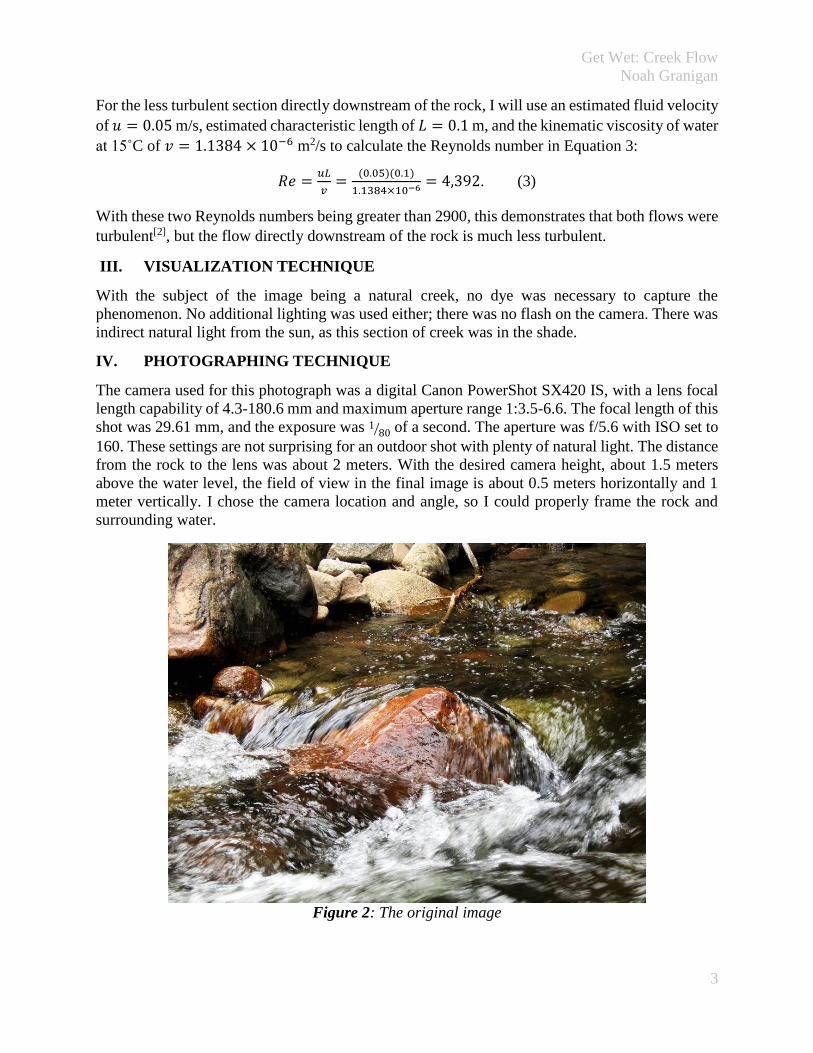
IV. PHOTOGRAPHING TECHNIQUE

The camera used for this photograph was a digital Canon PowerShot SX420 IS, with a lens focal

length capability of 4.3-180.6 mm and maximum aperture range 1:3.5-6.6. The focal length of this

shot was 29.61 mm, and the exposure was 1 80⁄ of a second. The aperture was f/5.6 with ISO set to

160. These settings are not surprising for an outdoor shot with plenty of natural light. The distance

from the rock to the lens was about 2 meters. With the desired camera height, about 1.5 meters

above the water level, the field of view in the final image is about 0.5 meters horizontally and 1

meter vertically. I chose the camera location and angle, so I could properly frame the rock and

surrounding water.

Figure 2: The original image

Get Wet: Creek Flow

Noah Granigan

4

The original image, Figure 2, had a size of 5152 × 3864 pixels, and the final image, Figure 4 seen

below, had an image size of 4865 × 2733

pixels due to cropping. I also chose to invert

the image, to get more vibrant colors that help

to distinguish the separation of the turbulent

and less turbulent areas. The curves were

adjusted as well, as shown in Figure 3. This

was done to distinguish the differences in flow

turbulence even more. I made the black areas,

which were more turbulent, blacker and the

white areas, which were less turbulent, whiter.

The contrast was also increased to 20 to help

visualize the different areas more.

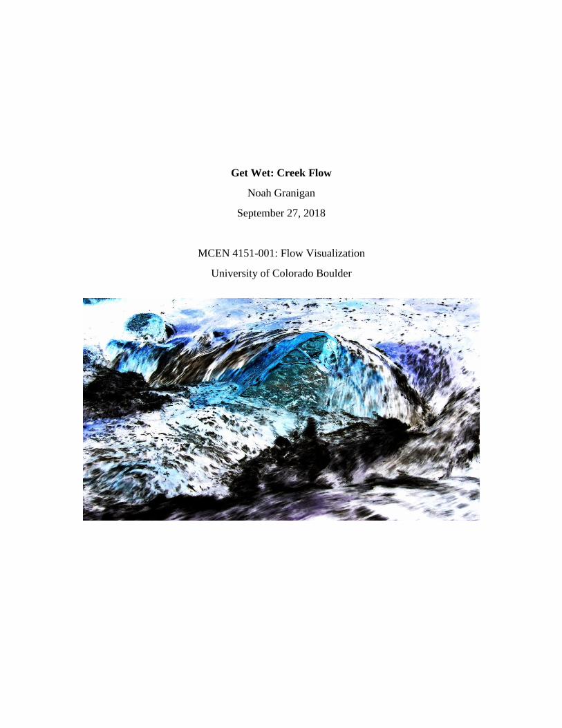
V. RESULTS

The final image, Figure 4, reveals the less turbulent flow that is “protected” by a rock in Boulder

Creek, contrasted to the increase in turbulence in the flow that is forced to the sides. In the image,

the black areas are more turbulent, and the white area is the less turbulent flow. This effect is called

an eddy. The physics of this phenomenon is demonstrated with the black and white colors

representing the more and less turbulent flows around the rock, respectively. I liked how I was

able to get such a great contrast of black and white flow areas, and how the inversion of the image

helped to demonstrate this. I believe that I was successful with this image, but in the future, I

would like to figure out a way to capture an eddy with the upstream effect clearly visible. I think

a video would be the best way to demonstrate this more clearly. With creek water in jeopardy of

not having clear enough water to use dies, I think dropping particles in the flow would convey the

properties of the flow in a much more digestible manner.

Figure 4: The final image, also shown on title page

Figure 3: Adjustments to the curves

Get Wet: Creek Flow

Noah Granigan

5

VI. REFERENCES

[1] Chiu, Jeng-Jiann, and Shu Chien. “Effects of Disturbed Flow on Vascular Endothelium:

Pathophysical Basis and Clinical Perspectives.” Physiological Reviews. vol. 91,

no.:1. Jan 2011, pp. 327-387. doi:10.1152/physrev.00047.2009. Accessed 19

Sep 2018.

[2] Gerhart, Philip M., et al. Munson, Young, and Okiishi’s Fundamentals of Fluid Mechanics.

8th ed., John Wiley & Sons, Inc. 2016.