Working Paper 05-79 (10) Dpto de Historia Económica e Instituciones Economic History and Institutions Series 10 Universidad Carlos III de Madrid December 2005 Calle Madrid, 126, 28903 Getafe (Spain)

Gerschenkron Revisited. European Patterns of Development in Historical Perspective?

Leandro Prados de la Escosura? Abstract_______________________________________________________________ Europe provides a suitable scenario for testing regularities of growth since its countries share to a large extent institutions, policies, and resource endowments. Patterns of development, that associate structural change to variations in GDP per head and population, are constructed for Europe in the nineteenth and the twentieth centuries along the lines of Chenery and Syrquin (1975) pathbreaking work. Thus, it is possible to discern whether a common set of development processes is observable for the whole continent and whether countries which had a late start exhibited, as posited by Gerschenkron (1962), a differential behaviour in terms of accumulation, resource allocation, and demographic transition. The results tend to confirm the different nature of latecomers’ development. JEL classification: N13, N14, O11 Keywords : patterns of development, modern Europe, latecomers, Gerschenkron

? I am indebted to Steve Broadberry, Giovanni Federico, and Moshe Syrquin for encouraging me to go back to a research project I initiated sometime ago. I have received valuable comments and suggestions on a previous version of the paper from Steve Broadberry, Giovanni Federico, Tim Hatton, Jaime Reis, Joan Rosés, Blanca Sánchez-Alonso, Isabel Sanz-Villarroya, James Simpson, and, especially, Patrick O’Brien. The usual disclaimer applies. ? Prados de la Escosura, Dpto de Historia Económica e Instituciones Universidad Carlos III de Madrid. E-mail: leandro.prados.delaescosura@uc3m.es

2 The search for an optimal path of development, usually associated to the German

Historical School, goes back to the Classical economists and can be traced back to the

philosophers of the Enlightenment 1. A stage approach to historical development was

suggested by Adam Smith, and Karl Marx quoted twice Horace's verses to emphasise

the extent to which Britain's industrialising experience forecasted the future of

Germany, by then, a late comer2. In the post-World War II years economists became

once more interested in long-term growth and turned to history searching for a

laboratory of natural experiments3. Stylised facts, short-cuts towards the optimal path of

development were explored during the Golden Age (1950-73) by a generation of

applied, historically minded economists.4 One of their achievements was the

construction of patterns of development that rely on theoretical findings but lack an a

priori model and, in the Clark/Kuznets tradition, are rooted in stylised facts.5 It is here,

where economic theorising does not provide an explanation that the contribution of

economic history is more needed.

Modern Europe provides a sound basis for testing empirical regularities of

growth as it offers a consistent and homogeneous set of countries which, to some extent,

have shared resource endowments, institutions, and economic policies. Nonetheless, the

map of Europe over the last two centuries shows, as Gerschenkron (1962, p. 353)

expressively put it, ‘a motley picture of countries varying with regard to the degree of

their backwardness’ and these initial differences have been ‘of crucial significance for

the nature of subsequent development’ as economic structure, institutions, and ideologies

all vary directly with them.6

In this paper it is my purpose to put the existence of a common path of

development in modern Europe to the test with the help of the stylised patterns of

structural change designed by Chenery and Syrquin (1975). However, Gerschenkron’s

(1962) emphasis on the fact that countries which had a late start would follow a

different path of development with respect to early starters will be taken on board. The

divergence between early starters and late comers originates in their structure of

production, that results, in turn, from different institutions that substituted for the 1 Cf. O'Brien (1975); Meier and Baldwin (1957), Schumpeter (1954). 2 Smith (1776); Marx (1867). Marx (1867, I, preface) writes, ‘the industrially more developed country presents to the less developed country a picture of the latter’s future’. 3 Cf. McCloskey (1981). 4 Clark (1940), Lewis (1954), Solow (1956, 1957), Gerschenkron (1962), Kuznets (1956/67, 1966, 1971), Chenery (1960, 1968, 1975), Rostow (1960), Denison (1962, 1967), pioneered a positive approach to the determinants of economic development. 5 That is, ‘income -related changes for which the available evidence suggests considerable uniformity but for which there is yet no well defined body of theory’ (Chenery and Syrquin, 1975, p. 6). 6 We cannot presume, therefore, that European nations went throughout similar stages of development á la Rostow (1960). Cf. the path breaking work of Patrick O’Brien and Çaglar Keyder (1978).

3 missing pre-requisites of the first wave of industrialization. 7 The existence of distinctive

development patterns for different epochs in Modern European history, such as the

liberal era prior to World War I, the neo-mercantilist Interwar Years, and the post-

World War II return to liberalism, will be, therefore, investigated, and by widening the

scope of the paper to include both the nineteenth and the twentieth century

Gerschenkron's qualifications about the distinctive paths of development followed by

early starters and latecomers will be revisited.8 It is worth stressing that the historical

approach in a relatively homogenous region, such as Europe, that combines cross-

section and time series data provides a superior choice to the usual cross-section

analysis for the recent past, in which low income countries are associated to early

phases of development regardless (over-time and cross-country) differences in

preferences and tastes.9

A Chenery and Syrquin Approach to European Development Patterns

Modern economic development is seen as an identifiable process of growth and

change whose main features are the same across countries (Solow 1977, p. 491)10 and

can be defined as ‘an interrelated set of long-run processes of structural transformation

that accompany growth’ (Syrquin 1988, p. 205).11 A structural transformation consists

of a set of changes in the composition of demand, production, trade, and employment,

each reflecting different aspects of shifts in resource allocation that takes place as

income levels rise. Thus, a development pattern may be defined as any systematic

variation in the economic and social structure associated to a rising level of per capita

income. Structural changes interact with the pattern of productivity growth in a general

equilibrium system to determine the rate and pace of growth (Syrquin 1986, pp. 436-

37).

7 As Chenery (1975, p. 458) pointed, ‘late comers are different.. [the difference] stems from the existence of the advanced countries as a source of technology, capital and manufactured imports, as well as markets for exports’. 8 The paper follows the lead established two decades ago by Irma Adelman and Cynthia Taft Morris (1984) and Nick Crafts (1984) to cover earlier epochs than the statistically convenient late twentieth century world, usually neglected by development economists. Crafts (1984, p. 449) already perceived in Nineteenth Century Europe Gerschenkronian ‘tendencies towards a different kind of structural change in the later developing countries’. 9 Cf. Branson, Guerrero, and Gunter (1998) for the latest substantive addition to this literature. 10 The rationale for this approach, as exposed by Kuznets (1959, p. 170), ‘is conditioned on the existence of common, transnational factors, and a mechanism of interaction among nations that will produce some systematic order in the way modern economic growth can be expected to spread around the world’. 11 A more comprehensive definition of economic development has been put forward by Adelman and Morris (1984, p. 46) as ‘the process of institutional transformation by which structural change is achieved and gains and losses are distributed’.

4 In the patterns of development framework, each country is treated as an

integrated, interdependent component of the international economy. Such an assumption

is only acceptable in Modern Europe after mid-nineteenth century, once the basis of the

liberal international order was established. By then, however, more than three centuries

of mercantilism, warfare and experience with internal and imperial markets had placed

the countries of Europe at rather diverse levels of development.

The patterns of development approach has been subjected to systematic

criticism12. It has been argued that Chenery-Syrquin equations derive from an

unspecified model of development in which we cannot tell supply from demand

determinants. Moreover, development patterns do not reveal a unique path to

industrialisation since comparative advantage, policy and institutions matter. A

country's trade and production patterns, as Bhagwati (1977, p. 491) reminded us, are

‘the result of an interaction between the country's own endowments and demands and

the rest-of-the-world's endowments and demands’, a fact apparently not accounted for

in the Chenery patterns. The challenge, therefore, would be, instead, to assess ‘the

ability of an economy to reach its full potential, that is, to come close to optimal growth’

(Williamson 1986). Another line of criticism relates to the econometric approach as

causality may run in either direction: from the level of per capita income to the

structural variable or vice-versa (Branson et al. 1998).

In the development patterns, however, there is no implication that a single

unique path, through which all economies have to pass, have to exist. On the contrary,

Chenery and his associates were always aware that, by treating development within a

uniform framework, systematic differences in development patterns among nations

would be identified.13 In fact, they distinguish between two components of a country's

pattern of development: the normal effect of universal factors (that accounts for most of

the observed structural variation among countries) and the effects of a country's

individual history (that can be more readily evaluated after allowing for the uniform

elements in each development pattern) (Chenery and Syrquin (1975, p. 5).

Nonetheless, the only feasible way to approach historical reality, as

Gerschenkron (1962) wrote, is through the search for certain regularities or

uniformities, and the analysis of deviations to the norm. Since development occurs with

sufficient uniformity among countries to produce a consistent pattern of change in

12 Cf. for instance, Díaz Alejandro (1976) and Perkins (1981). Williamson (1986) wrote, “in uncritical moments we tend to gauge an economy’s performance by its ability to replicate or even exceed those stylized patterns”. 13 As Chenery (1988, p. 60) put it, “the search for uniform features of development almost inevitably leads to a division of countries into more homogeneous groups”.

5 resource allocation, factor use, and other structural features as the level of per capita

income rises, a set of basic processes only restricted by the lack of empirical evidence

has been selected14. All variables are expressed as shares (of GDP, total employment,

etc.) since it is the relative variation which determines structural change. Shares are

calculated at nominal prices since the decisions of individuals and firms are more

meaningfully analysed at current, rather than at constant, prices. The development

processes studied can be divided into three main categories: a) accumulation, that deals

with the resources used to increase an economy's productive capacity, for which we

have gathered information on stocks (literacy) and on increases in stocks (gross

domestic investment and school enrolment); b) resource allocation, which interacting

with accumulation, produces systematic changes in the composition of domestic

demand, foreign trade, production, and employment, as real product per head rises15 ; c)

demographic transition. Here they are summarized:

1. Domestic Demand (percentage of GDP): gross domestic investment, private

consumption, and government consumption.

2. Education: primary and secondary school enrolment (percentage of population aged 5

to 19) and literacy (percentage of population over 7 years old).

3. Output Structure (percentage of GDP): value added in agriculture, industry (including

mining, construction and utilities), and services.

4. Labour Allocation (percentage of total labour force): labour force in agriculture,

industry, and services.

5. Foreign Trade (percentage of GDP): exports, imports, openness (exports plus

imports), primary exports, manufactured exports.

6. Urbanization (percentage of population in towns over 20,000 inhabitants).

7. Demographic transition: crude birth and death rates (per thousand inhabitants), gross

fertility (children per woman), infant mortality (per thousand births), net fertility16.

Data on structural change across Europe have been gathered mostly from

national sources, in particular, from reconstructed national accounts (see Appendix on

sources) for three year averages around years ending in 0 up to 1900; then, for

significant benchmarks in the Interwar period (1913, 1925, 1929, 1933, 1938) and for

years ending in 0 and 5 over 1950-90. A major feature of the data set is that non-market

economies have been excluded given the conceptual and data problems involved

14 Chenery and Syrquin (1975, p. 11). In a next version of the paper additional structural variables (financial, monetary, and social) will be added. 15As Chenery and Syrquin (1975, p. 33) put it, “theses patterns result from the interaction between the demand effects of rising income and the supply effect of changes in factor proportions and technology”. 16 Net fertility = (1 - infant mortality rate) ? gross fertility.

6 (different economic categories, low reliability, and, especially, a different set of

incentives for economic agents).

GDP per head is expressed here in 1990 U.S. dollars (converted at the Geary-

Khamis purchasing power parity) and countries’ series have been built by projecting

backwards 1990 levels (calculated at international prices) with each country growth

rates (estimated at national prices) and, regrettably, the resulting series suffer from a

serious index number problem since their economic meaning weakens as we move away

from the 1990 benchmark (Prados de la Escosura 2000).

Methodology

In this section the econometric methods used for the construction of patterns of

development are exposed. We start from the method designed by Chenery and Syrquin

(1975), and since the statistical procedure has to be applied to a wide range of structural

processes and countries, the scope for a more refined econometric specification is

constrained by the availability of data.17

In addition to confirming the existence of patterns of development common to

modern Europe, a major goal of this essay is to separate the effects of universal factors,

common to all countries, from particular characteristics of each one, in order to

highlight national deviations from the European patterns of development. I, therefore,

assume that any indicator of structural change, Iit, for i= country, and t= time period,

can be divided into two different parts:

I f U f Vit it i it? ?1 2? ?, , (1)

where, ? is a k? 1 vector of time and cross-country invariant parameters; Uit is a vector

of explanatory variables representing the level of development, market size, economies

of scale, etc. in country i at period t; ? i is a time invariant but cross-country variant

vector of parameters; and Vit represents a set of explanatory variables, including a

stochastic disturbance (which incorporates war, political unification, etc.). Uit includes

the explanatory variables in Chenery and Syrquin (1975), to which others for country

size and a time-trend component have been added:

U'it= [c, LnYit, (LnYit)2, LnNit, (LnNit)

2, INFLit, LnSizei, TRENDt] (2)

where c is a constant term; Yit, real income per head; Nit, population; INFLit, net

imports as a share of GDP; Sizei, country i's extension in square kilometres; TRENDt,

time trend dummy. 17 Branson et al. (1998) faced the same constraint for the last quarter of the twentieth century.

7 Under these conditions, f1(? ,Uit) will be the part of the structural variable Iit

that can be explained by the pattern of development common to all countries, while the

divergence of country i from the pattern will be f2(? i,Vit). Then, assuming that ?

exists amounts to accepting that a common pattern does exist. Next the necessary

assumptions to estimate the patterns of development properly have to be established. I

have preferred the semi- log to the double- log formulation in order to retain the additive

property for the different components of aggregates (i.e., sectoral shares of output must

add to 100). In addition, it will be assumed that f1(? ,Uit)=? *Uit. Under these

conditions, we have:

Ii t = ? 0 + ? 1* LnYi t + ? 2* LnYi t2 + ? 3* LnNit + ? 4* LnNi t

2 + ? 5* INFLi t

+ ? 6* LnSIZEi + ? 6* LnTRENDi + f2 (? i, Vi t) (3)

Following Chenery and Syrquin (1975) income per head works as an overall

index of development and as a measure of output. Population represents the market size

and captures the effect of economies of scale and transport costs on patterns of

production and trade. These effects are independent of the income level, since no

correlation is expected between market size and level. In addition, quadratic terms are

included to allow for non- linearities. In our sample, each country's population size

changes substantially as our time coverage is of one and a half centuries, and a new

country-size variable that represents the surface of the country helps to control for it,

while it works at the same time as a country-dummy. The time-trend variable should

capture universal changes over time not associated with the other independent variables

(e.g., institutions, policies, etc.) that affect all countries alike. The time-trend dummy

eliminates all variation between time periods so that the original panel data sample can

easily be treated like a simple pool of cross-section data, as regards the econometric

approach.

The target now will be to estimate the ? ? ? ?0 1 2 7, , , . . . vector. For this

estimate to be consistent, I will assume that there is no correlation between variables

included in Uit and Vit. This is a very strong assumption that may not be true in

practice and, therefore, one must be very cautious when interpreting the econometric

results.18 If such an assumption holds true, I will be able to isolate additively and

18 To avoid this problem, it could have been assumed that Vit = Vi , ? t and f2 (ßi,Vi)= ß i’*V

i. This linear

specification would permit to eliminate the term f2 (ßi,Vi) taking deviations with respect to the mean in the time-varying dimension (within-group estimator). But, in that case, I would also get rid of a0. This would not be present a major problem if I were sure that a0 is really a constant because, in such a case several estimation techniques could be used consistently. However, it is easy to guess that a0 will present several structural changes in its long time -varying dimension, and testing this hypothesis is another goal of this

8 consistently the part of the structural variable that can be explained by a common

pattern of development, and obtain f2(? i,Vit) as a residual that measures the particular

divergence of each country's structural indicator from the pattern.

The formulation described so far is what I will call the single pattern because the time-

varying regressors are supposed to have homogeneous effects on each structural

variable over the whole time span. A second and more historically relevant approach

has been introduced to test and, in its case, to detect the existence of structural changes

in the constant term and in the slopes of LnY and LnN in different sub-periods of our

sample. This method allows us to go beyond the time-trend dummy that stands for an

exogenous uniform shift but is unable to discriminate among periods (Chenery and

Syrquin 1975, p. 154). The outcome is the adjusted pattern. Three historical periods

were chosen to test structural breaks: the period prior to World War I, the Interwar

years, 1920-1938, and the post-World War II period up to 1990.19 To allow for different

possibilities of structural change over these historical periods, dummy variables are

defined in Table 1.

Regression Analysis

The econometric results for both single and adjusted patterns, presented in the

Appendix, deserve some comments. The main finding is that existence of patterns of

development common to modern European countries appears to be confirmed. Adjusted

R squared and statistical tests indicate so. If accumulation and resource allocation

processes are examined we can find, for example, that as regards the composition of

demand, both coefficients of income and population present the expected sign, as

income is negatively related to consumption (total and private) and positively to

domestic investment, while the opposite occurs to population. Size and trend dummies

also correlate positively to investment and negatively to consumption (only to private

consumption for the time trend). Larger countries appear to invest more at given levels

of income and investment rates increase as time goes by, regardless of income (while

the opposite happens to private consumption). In the adjusted patterns, a dummy

variable for the slope of LnY in different periods allow us to locate structural breaks,

essay. For such a reason, I finally decided to assume the lack of correlation between Uit and Vit, and to go on with the initial specification. 19 The choice of 1990 as the end year in this investigation is due to the fact that the demise of communism in Europe changed borders and was followed by a transition to the market in central and eastern European countries that have not been taken on board while they were command economies and accumulation and resource allocation were not ruled by market forces. Thus, this paper cover the late nineteenth century (1850-1913) and, to use Hobsbawn’s expression, ‘the short’ twentieth century (1914-1990).

9 from which emerges that, for investment, as it could be expected, the estimated

coefficient of income reached the highest value in the post-World War II era, and the

lowest in the interwar years. The same happens (but with a negative sign) to private

consumption, with larger absolute values for the post-1950 period, and a positive

coefficient for the interwar years.

The supply side offers the expected correlation between income and population

on the one hand, and agricultural shares in output and employment on the other, i.e.,

negative for income and positive for population, while a positive one appears for

industry shares in output and employment with respect to income 20. When the estimated

coefficient on the quadratic term shows an opposite sign to that of the linear term, it

means that the relation between structural change and income level attenuates as GDP

per head rises. The time-trend and size dummies show a positive sign for agricultural

shares in output and employment, independently from the level of income (while the

opposite is observed for industry). In the case of agriculture, the estimated coefficient

for income, negative, is higher in absolute terms for the period prior to World War I (as

the adjusted coefficients reveal).

Urbanization, as expected, is positively related to income and population and

also to net imports (a proxy for capital inflow), while is negatively correlated to the

country's size. Human capital indicators (school enrolment and literacy) consistently

show positive correlations with income and negative ones to population and size. The

time trend appears to be positive for primary and secondary schooling although the

income coefficient was higher before World War I.

The demographic transition shows the expected negative relation to income for

birth and death (including infant mortality). For the adjusted pattern, fertility (both gross

and net) is positively related to income. Such a result suggests that findings for the post-

1960 world, i.e., a negative relation between net fertility and income (Barro

(1991,422)), cannot be simply extrapolated to earlier periods in which economic

development helped to reduce infant mortality and, therefore, increased net fertility. A

clear negative time trend appears for all demographic indicators.

Finally, foreign trade indicators unanimous ly show a positive relation to income

(with larger estimated coefficients as time goes by), and a negative one to population

and size, as well as a negative time trend which suggests that latecomers tend to be less

20 When quadratic terms exist, the resulting overall value has been obtained by weighting coefficients for quadratic and non quadratic terms with income values ranging from 1,000 to 15,000 US dollars at 1990 prices (PPP). Not clear relationship appears for population and industry shares in output and employment (positive for the single pattern, negative for the adjusted pattern). For services shares, there is a negative correlation for population, while for income it is only negative for the single pattern.

10 open at similar income levels. The positive link between population and manufacturing

exports is the exception and might suggest a Linder's (1961) scenario of representative

demand, in which producing industrial goods for home consumption appears as a pre-

requisite for exporting them.

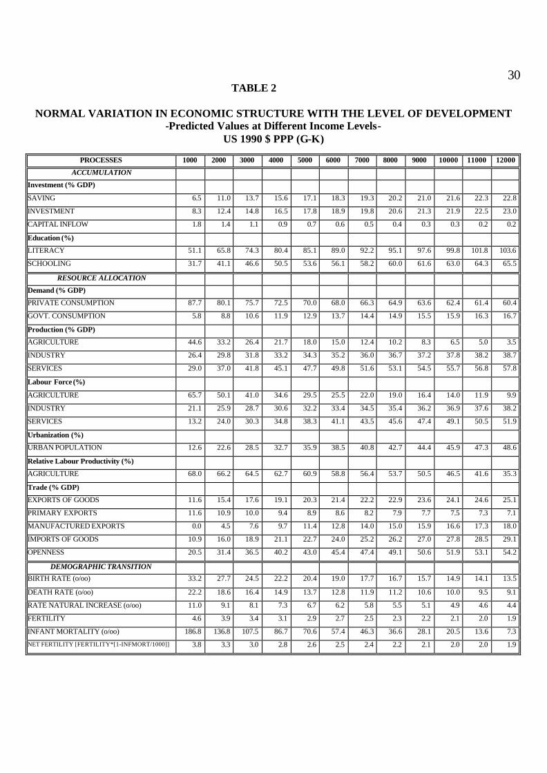
Normal Structural Variation with the Level of Development

Table 2 presents the structural transformation that occurs as real GDP per head

grows. Simulations are provided for all development processes within an income range

from 1,000 to 12,000 dollars (at 1990 ‘international’ prices (PPP)), when most of the

transition from a pre- industrial to a modern society occurs. Three development

processes are considered, i.e., accumulation, resource allocation, and demographic

transition. Together with the normal structural change associated to a rise in GDP per

head, growth elasticities have been computed for given levels of per capita income and

its changes (Table 3).

Most development processes were half-completed at early stages of

development, somewhere in between 3,000 and 4,000 dollars, and four-fifths of the

transformation had occurred by a 8,000 dollar income21. The implication is that growth

in post-World War II Europe, the period from where most economic theorists derived

their stylised facts, is weakly related to resource allocation22.

In the accumulation process, proxies for physical and human capital have been

considered. Information on GDP expenditure components permitted to derive net

imports of goods and services as a residual which, in turn, proxied capital net inflow,

and, as a result, to derive the rate of national saving (expressed as a share of GDP). The

comparison between investment and saving suggests a life-cycle behaviour, in which

domestic saving is lower than investment demand at initial levels of the trans ition, with

the gap closing as income rises. In both cases, the share of GDP increases as income

rises, multiplying over the total income range considered by a ratio of 3.5 in the case of

saving (2.4 times up to $4,000, the mid- transition point), and by 2.8 in the case of

investment (2.0 up to $4,000), that is, representing a gain of 16.3 percentage points for

saving, and 14.7 for investment (9.1 and 8.2 by $4,000, when half the transition was

completed). Proximate indices for human capital also show large increases, multiplying

21 Pro-memoria, A per capita income of $4,000 was reached by the U.K. in the 1890s, and by France in the mid-1920's; a level of $8,000 was reached by the UK or Germany in the early 1960s; and $12,000 was the income of France and Germany in the early 1970s (Maddison 2003). 22 Such an empirical fact reinforced perhaps the neoclassical assumption that adjustments within the economy were immediate and frictionless.

11 by 2 over the transition (1.6 by half of it), that is, up to 52.5 percentage points for

literacy, and 33.8 for schooling, (29.3 and 18.8 up to $4,000).

Associated to growth, there are structural shifts in the allocation of resources.

Resource allocation interacts with factor endowments, economic policies and

productivity growth to condition the path of development. We can analyse demand and

supply changes separately. Overall consumption fell by 20 per cent throughout the

transition (10 per cent when half of it was achieved), that is, declining from over 90 per

cent of aggregate demand to around three-fourths. Trends in private and government

consumption followed, however, opposite directions, while the former fell by 31 per

cent, the latter rose by 188 per cent (-17 and 105 per cent, respectively, over the first

half of the transition). In percentage points, the variations represent 27.3 percentage

points of decline for private and 10.9 of rise for public consumption (-15.2 and 6.1 by

half the transition).

On the supply side, a decline occurs in agriculture's shares in output and

employment, while, for industry and services, there is an increase. It is worth

mentioning that absolute increases are more noticeably in the shares of services (28.8

and 38.7 percentage points gained for output and employment, respectively, over the

transition) than for industry (12.1 and 17.1, respectively), in particular, at higher income

levels (over $4,000). Agriculture's supremacy in output and employment disappears by

$3,000, and $4,000, respectively. Interestingly enough, the proportional change implied

by the transition differs from output to employment. It means that relative (average)

labour productivity (that is, the ratio of each sector’s share in output to that in

employment) differs across sectors and, consequently, that efficiency improvements in

the use of labour do not proceed at the same pace across sectors. In agriculture, a

sharper decline can be noticed for its output's share (-41.1 percentage points) than for its

employment's share (-55.8) (where a relative and, then, an absolute decline is

experienced), which explains why the productivity gap widens as income rises. The

lagged shift of labour out of agriculture due to low mobility of the workforce, as it is the

case when surplus labour in agriculture exists, contributes to explaining the productivity

gap. Besides, partial productivity differences appear in most industrialization

experiences as investment and technological change occur more often in modern

industry and services23. Had all sectors the same production function, average labour

productivity would equalise across them, provided the same factor prices and a

complete resource mobility for all (Chenery 1988, p. 256). Data constraints, however,

23 Cf. Chenery and Syrquin (1975, p. 48).

12 do not allow me to address differentials in marginal productivity. A caveat to be made

about relative labour productivity derives from the weakness of statistical data for

employment in agriculture. In fact, at lower income levels, when the division of labour

is not widely diffused yet, figures for economically active population in agriculture (the

main historical source for employment) tend to be over-exaggerated, as part-time

labourers in industry and services tend to register under their main professions, e.g.,

farmers and, hence, figures for industry and services understated24.

The share of population living in towns over 20,000 inhabitants is the arbitrary

threshold used here to assess the degree of urbanization. A rapid increase in

urbanization takes place as income rises. A multiplier of 3.9 applies for the entire

transition (2.6 for half of it), representing a 36 percentage point rise (20 up to $4,000).

Besides, a decline in the proportion of agricultural labour within rural population

(measured as the ratio of the agricultural share in total employment to the rural share in

total population) occurs as GDP per head improves, suggesting that people living in the

countryside tends to work increasingly outside agriculture as economic growth proceeds

(from three quarters to one-fifth over the transition).

Development patterns for international trade help us to search for the sources of

a country's comparative advantage and its changes as income grows. Historically,

natural resource endowments, factor proportions, and economic policies have

conditioned trade specialisation. Examination of trade patterns shows a close link

between the rise in GDP per head and that in trade ratio to GDP (33.7 percentage point

gain for openness, that is, exports plus imports), though the gain of imports exceeds that

of exports. A possible explanation for the latter would be that as their income grow,

countries become competitive in services, as in nineteenth century Century Britain

(Imlah 1958) or attractive to foreign capital, as Spain in the 1860s-1880s (Prados de la

Escosura 2005). Changes in comparative advantage from primary production to

manufacturing are revealed by the composition of exports as income grows.

Manufactured exports overcome those of primary goods around $4,000 of income.

Meanwhile, industry's share in GDP becomes larger than agriculture's at $3,000. Such a

lag suggests that, in Europe, the emergence of a domestic market for industrial goods is

previous to that of foreign markets.

Finally, the demographic transition suggests a decline in both natality and

mortality, in which the former experienced a deeper absolute fall, with the result of a

24 Cf. Federico (2005) and O'Brien and Prados de la Escosura (1992). Adjustment for actual days worked would further reduce the size of labour force in agriculture. Cf. Prados de la Escosura and Rosés (2005) for an exploration of the Spanish case.

13 slowing down in the rate of natural increase (by 6.6 percentage points), as income per

head improves. Meanwhile, a decline in gross fertility is softened in net terms by the

more rapid reduction in infant mortality.

So far only tendencies have been pointed out. Table 3 provides a more precise

measurement of the responsiveness of structural transformation to changes in GDP per

head for each development process. Elasticities have been computed both at a given

level of per capita income (point estimates) and for income changes (discrete estimates),

covering most of the transition from a pre- industrial into a modern economy. It appears

that, in both estimates, the lower the income level, the higher the value of the coefficient

for growth elasticity, with the exception of those cases in which a negative relationship

exists, where the opposite occurs. Differences in the structural response to increases in

income are worth noticing. Both measures of (absolute) elasticities are higher, at low

income levels, for investment and government consumption, the share of services in

total employment and urbanization and manufactured exports, while the opposite occurs

for agriculture’s shares in output and employment, fertility (gross and net), infant

mortality and crude birth and death rates.

Early Starters and Latecomers

Up to this point, the discussion has been carried out on the basis of development

patterns common to Modern Europe over one and a half centuries. However, when one

and a half centuries is being considered, distinctive structural behaviour at different

historical periods should be expected. The adjusted patterns of development allow for

historical differences in structural change across different phases (up to World War I, in

the Interwar years, and in the post-World War II era) and, therefore, help to

distinguishing the features of early starters and late comers. A similar approach to the

one used in the construction of average single patterns has been followed for the

adjusted patterns. Table 4 presents the patterns, while growth elasticities appear in Table

5. For the sake of simplicity, only the $1,000- $4,000 income range has been considered

as, actually, most European countries had not reached the upper level by 1913.

Gerschenkron provided a set of propositions that can be tested with the help of

the adjusted development patterns. Thus, he asserted that, the more backwards a country

is, a) the faster the growth of industrial output; b) more intense the stress on bigness of

both industrial plant and enterprise; c) the greater the stress upon producers’ goods; d)

the stronger the pressure on private consumption levels; e) the greater the role of

institutional factors in promoting industrialization (banks, the State), and f) the less

14 active the role of agriculture in industrialization, that is, its provision of a market for

industry by rising labour productivity (Gerschenkron 1962, pp. 353-54).25

Unfortunately, only some of Gerschenkron's hypotheses about European

development can be subjected to quantitative testing: The evidence presented here

provides an empirical test if we associate proposition a), to the size (and the increases)

in the share of industry in output and employment; hypotheses b), c) and d) to the

shares of GDP allocated to investment and private consumption, respectively;

proposition e), to the share of GDP assigned to government consumption, and, finally,

hypothesis f) to the productivity gap and the relative size of agriculture in GDP and

labour force.

From the comparison between Pre-World War I and the average single patterns

of development for 19th and 20th centuries some interesting findings can be reported.

As regards propositions b) and c), accumulation in both human and physical capital

proceeded at a different pace before the Great War (Table 4); it was larger at low

income levels and smaller at high ones, i.e., pre-1914 investment was higher below a

per capita income of $2,000, as it was the case of literacy and schooling below a $3,000

income. Thus, the lower investment rates in physical and human capital for the late

nineteenth and early twentieth century provides support to Gerschenkron’s content ion of

latecomers’ emphasis on producers’ goods.

Differences observed for resource allocation processes offer an answer to

propositions d) and e). Thus, the composition of expenditure prior to World War I

points to a higher (overall) consumption over $2,000, with the share of private

consumption larger and that of government consumption smaller above $1,000. It

means that early starters suffer from a lower pressure on private consumption while the

size of Government, usually correlated to its activist role, was smaller, as

Gerschenkron’s asserted.

The supply side shows noticeable differences for the pre-1914 patterns and

provides responses to propositions a) and f). Before the Great War, European

agriculture presents a larger size of GDP for any income level, and a smaller labour

force over a $1,000 income, than the average single pattern. As a result, a lower

productivity gap emerges, which tends to close as income rises. In other words, early

starters exhibit a smaller agriculture in terms of employment and a larger size in terms

of output and, hence, relative average labour productivity in agriculture was higher than

in the case of the late comers. The lagged shift of labour out of agriculture and its higher

25 A critical assessment of Gerschenkron's views can be found in O'Brien (1986). Gerschenkron's views are examined in the light of research during the late twentieth century in Sylla and Toniolo (1992).

15 productivity gap confirm Gerschenkron's (1962) contention that late comers’ agriculture

had a less active role in economic growth.

Industry and services lower shares in GDP (the latter up to $3,000) and higher

ones in employment (over $1,000 in the case of industry) complete a more balanced

labour allocation prior to the Great War. Besides, a more urbanized society and a

smaller proportion of its rural population involved in agricultural activities appears

above $2,000 in the pre-World War I patterns. However, in the case of the latecomers,

the relative size of industrial output grew faster within the same income range,

supporting Gerschenkron’s contention of more intense industrial growth in the case of

latecomers.

Differences in international trade also appear between average and pre-World

War I patterns of development, as the latter exhibits a more open economy over $1,000

in which the larger share of manufacturing exports reveals its comparative advantage.

The systematic commodity trade surplus in early starters in contrast with the deficit in

latecomers (that emerges from the average, single, pattern) points to a higher investment

demand than domestic saving in the case of latecomers while the opposite appears to

occur in that of early starters (nineteenth century Britain and France provide good

examples) (Imlah, 1958; Lévy-Leboyer, 1978).

Higher birth and death rates, and lower population pressure below $4,000, plus

higher fertility and infant mortality, are the main demographic differences for pre-1914

Europe when compared with average, single patterns.

Comparing growth elasticities for each structural variable at given income

levels, or as income increases for different historical phases, is most illuminating.

Values (in absolute terms) for both measures of elasticity for the pre-World War I era

are shown in Table 5. The comparison with those of elasticities for the average patterns

of development (Table 3) indicates that, in the income range $1,000-4,000 lower values

are found for both the shares of investment and of industry in GDP. It might be

suggested that such a result is associated to latecomers’ catching up with early starters

and lends support to Gerschenkron’s propositions a), b), and c). Nonetheless, larger

growth elasticity for human capital formation and for openness, two ingredients of

successful industrialization, are exhibited in the pre-World War I patterns. Moreover, a

much lower value of the growth elasticity for Government consumption in early starters

tends to confirm the idea of the State’s stronger stand in latecomers. Finally, the higher

(absolute) value of the growth elasticity for the agricultural share in employment and for

the urbanization rate among the early starters reinforces the view of a less dynamic rural

sector in the case of latecomers.

16 It can be inferred, then, that Gerschenkron's stylised patterns of European

development are not rejected by the empirical evidence provided here.

Concluding Remarks

In this paper European development patterns that associate structural change to

variations in GDP per head and population have been examined in historical

perspective. Europe provides a suitable scenario for testing regularities of growth since

its nations share a common set of institutions, policies, and resource endowments. Some

lessons can be derived.

Patterns of structural change, constructed along the lines of Chenery and Syrquin

(1975) pathbreaking work, confirm the existence of a common set of development

processes associated to rising per capita income for the whole of Europe. However,

discernable development patterns for different epochs (observed with the adjusted

patterns) confirm Gerschenkron’s (1962) perception that early starters and latecomers

followed their own paths of economic modernization.

Differences between stylised features of development in early starters and

latecomers raise interesting questions for further research. Are latecomers penalised by

the fact that, at the same level of income per head, their investment and consumption

shares of GDP are larger and lower, respectively, than for an early starter? Or do such

differences, actually, result from a wider range of investment opportunities?.26

Demonstration effects and the awareness that a higher rate of investment helps to catch-

up are perhaps behind such a differential. As Gerschenkron (1962, p. 8) put it, ‘the

opportunities inherent in industrialization (..) vary directly with the backwardness of the

country’.

Chenery and Syrquin (1975, p.64) reminded us that ‘the analysis of the

uniformity of development patterns constitutes a first step towards identifying the

sources of diversity’. Each country's deviations from the estimated patterns at a given

level of income per head and population, are associated to country-specific

characteristics such as resource endowments, institutions, and policies, and the extent to

which such a differential behaviour in accumulation, resource allocation, and

demographic transition is behind the distinctive performance of latecomers deserves to

be fully investigated within the framework of modern growth literature.

26 Chenery (1977, p. 458). Besides, in recent times larger investment seems to be required to reach economies of scale and scope in modern industry and services.

17 REFERENCES

ADELMAN, I. and C. T. MORRIS (1984). Patterns of Economic Growth, 1850-

1914, or Chenery-Syrquin in Historical Perspective. In M. Syrquin, L Taylor and L.

E. Westphal (eds), Economic Structure and Performance, Essays in Honor of Hollis

B. Chenery. San Diego: Academic Press, pp. 45-74.

BAKKER, G.P. den, T.A. HUITKER and C.A. van BOCHOVE (1990). The Dutch

Economy 1921-1938: Revised Macroeconomic Data for the Interwar Period Review

of Income and Wealth 36, pp. 187-206.

BAIROCH, P. (1976). Commerce extérieur et développement économique de l'Europe

au XIX e siècle. Paris: Mouton.

BAIROCH, P., T. DELDYCKE, H. GELDERS, and J.-M. LIMBOR (1968). The

Working Population and its Structure. Brussels and New York.

BALDWIN, R.E. (1958). The Commodity Composition of Trade: Selected

Industrial Countries, 1900-1954 Review of Economics and Statistics, 40, pp. 50-71.

BARRO, R.J. (1989). A Cross-Country Study of Growth, Saving and Government.

NBER, Working Paper 2855.

BARRO, R.J. (1991). Economic Growth in a Cross Section of Countries Quarterly

Journal of Economics 106, pp. 407-43.

BATCHELOR, R.A, R. L. MAJOR and A. D. MORGAN (1980). Industrialisation and

the Basis for Trade. The National Institute of Economic and Social Research. Cambridge:

Cambridge University Press.

BATISTA, D., C. MARTINS, M. PINHEIRO and J. REIS (1997). New Estimates of

Portugal’s GDP 1910-1958. Lisbon: Banco de Portugal.

BHAGWATI, J.N. (1977). ‘Comment’ to H. B. Chenery, ‘Transitional Growth and

World Industrialization’. In B. Ohlin et al. (eds), The International Allocation of

Economic Activity. London: Macmillan, pp. 496-98.

BRANSON, W.H., I. GUERRERO, and B.G. GUNTER (1998). Patterns of

Development, 1970-1994, World Bank Working Paper.

BUYST, E. (1997). New GNP Estimates for the Belgian Economy during the Interwar

Period Review of Income and Wealth 43, pp. 357-75.

CAPANNA, A. and O. MESSORI. (1940). Gli scambi commercials dell'Italia con

1'estero. Roma.

CARRE, J.J., P. DUBOIS and E. MALINVAUD (1976). French Economic Growth.

Oxford: Oxford University Press.

18 CARRERAS, A., ed. (1989). Estadísticas Históricas de España, Siglos XIX—XX. Madrid:

Fundación Banco Exterior.

CARTAXO, R.J. and DA ROSA, N.E. (1986). Series longas para as contas nacionais

portuguesas 1958-1985, Banco do Portugal, Documento de Trabalho 15.

CHENERY, H.B.(1960). Patterns of Industrial Growth American Economic Review

50, pp. 624- 54.

CHENERY, H.B. (1986a). Growth and Transformation. In H.B. Chenery, S.

Robinson and M. Syrquin (eds), Industrialization and Growth. New York: Oxford

University Press, pp.13-36.

CHENERY, H.B. (1986b). Structural Transformation: A Program of Research. In G.

Ranis and T.P. Schultz (eds), The State of Development Economics. Progress and

Perspectives. Oxford: Basil Blackwell, pp. 49-77.

CHENERY, H.B. (1988). Introduction to Part II: Structural Transformation. In H. B.

Chenery and T. N. Srinivasan (eds), Handbook of Development Economics, 2 vols.

Amsterdam: North-Holland, vol. I, pp. 197-202.

CHENERY, H.B. and SYRQUIN, M. (1975). Patterns of Development, 1950-1970.

Oxford: Oxford University Press.

CHENERY, H.B. and L. TAYLOR (1968). Development Patterns: Among Countries

and Over Time Review of Economics and Statistics 50, pp. 391-416.

CHESNAIS, J.C. (1986). La transition démographique. Institut National d'Études

Démographiques. Travaux et documents, Cahier no. 113. Paris: Presses

Universitaires de France.

CLARK, C. (1940), The Conditions of Economic Progress . London: Macmillan.

DENISON, E.F. (1967). Why Growth Rates Differ. Postwar Experience in Nine Countries.

Washington, D.C.: The Brookings Institution

DEUTSCH, K.W. and ECKSTEIN, A. (1961). National Industrialization and the

Declining Share of the International Economic Sector, 1890-1959. World Politics 13,

pp. 267-299.

DIAZ ALEJANDRO, C. (1976). Review of Patterns of Development 1950-1970.

by M. Chenery and M. Syrquin Economic Journal 86, pp. 401-3.

DOWRICK, S. and N. GEMMELL (1991). Industrialisation, Catching up and Economic

Growth: A Comparative Study Across The World's Capitalist Economies Economic

Journal 101, pp.. 263-75

ECKSTEIN, A. (1955). National Income and Capital Formation in Hungary, 1900-1950

Income and Wealth V, pp. 150-223.

19 EDDIE, S. (1977). The Terms and Patterns of Hungarian Foreign Trade, 1889-1913

Journal of Economic History 37, pp. 329-58.

EICHENGREEN, B. (1986). What Have We Learned from Historical Comparison of

Income and Productivity?. In P. O'Brien (ed), International Productivity Comparisons and

Problems of Measurement, 1750-1939. Ninth International Economic History, Bern, pp.

26-35.

ERCOLANI, P. (1978). Documentazione statistica di base. In G. Fua (ed), Lo sviluppo

economico in Italia, III, pp. 388-472.

FEINSTEIN, C. M. (1972). National Income, Expenditure and Output of the UK, 1855-

1965. Cambridge: Cambridge University Press.

FEDER, G. (1986). Growth in Semi-Industrial Countries: A Statistical Analysis. In H. B.

Chenery, S. Robinson and M. Syrquin (eds), Industrialisation and Economic Growth. New

York: Oxford University Press, pp. 263-82.

FEDERICO, G. (2005). Feeding the World. An Economic History of Agriculture, 1800-

2000. Princeton and Oxford: Princeton University Press.

FEENY, D. (1987). The Explanation of Economic Changes: The Contribution of

Economic History to Development Economics. In A. J. Field (ed), The Future of Economic

History. Boston: Kluwer Nijhoff, pp. 91-119.

FLORA, P. (1973). Historical Process of Social Mobilization: Urbanization and Literacy,

1850-1965. In S.N. Eisenstadt and S. Rokker (eds), Building State and Nation, pp 213-58.

FLORA, P (1987). State, Economy and Society in Western Europe, 1815-1975. Frankfurt:

Campus Verlag GmbM.

FREMDLING, R. (1988). German National Accounts for the 19th and Early 20th

Century. A Critical Assesment Vierte jahrschrift fair Social- and Wirtschaftsgeschichtes,

75, pp. 339-55.

FUA, G. (1978-81). Lo sviluppo economico in Italia. Storia dell' economia italiana negli

ultimi ciento anni. Milano: Franco Angeli, 3 vols.

GERSCHENKRON, A. (1962). Economic Backwardness in Historical Perspective. A Book

of Essays. Cambridge: Harvard University Press.

GOOD, D.F. (1994). The Economic Lag of Central and Eastern Europe: Income

Estimates for the Habsburg Succesor States, 1870-1910 Journal of Economic History

54, pp. 869-91.

GREGORY, P. (1982). Russian National Income. Cambridge: Cambridge University

Press.

HANSEN, S.A. (1974). Økonomisk vœkst i Danmark. Copenhagen: Akademisk Forlag.

20 HAYAMI, Y. and RUTTAN, W.V. (1985). Agricultural Development. An International

Perspective. Baltimore: The Johns Hopkins University Press.

HJEERPE, R. (1988). The Finnish Economy, 1860-1985. Growth and Structural Change.

Helsinki: Bank of Finland.

HJERPPE, R. (1994). Finland's Historical National Accounts 1860-1994: Calculation

Methods and Statistical Tables. Jyväskylä: J.Y.H.L.

HODNE, F. and O.H. GRYTTEN (1994). Gross Domestic Product of Norway 1835-

1915. Occasional Papers in Economic History, Umea University.

HOFFMANN, W.G.(1965). Das Wachstum der Deutschen Wirtschaft seit der Mitte des

19.Jahrhunderts. Berlin: Springer.

HORLINGS, E. (1997). The Contribution of the Service Sector to Gross Domestic

Product in Belgium, 1835-1990. Universiteit Utrecht (mimeo).

IMLAH, A.H. (1958). Economic Elements in the Pax Britannica. Studies in British Foreign

Trade in the XIXth Century. Harvard: Harvard University Press.

JUSTINO, D. (1987). A evoluçâo do Producto Nacional Bruto em Portugal, 1850-1910.

Algunas estimativas provisorias Análise Social 23, pp. 451-61.

KAUSEL, A. (1979). Österreichs Volkseinkommen 1830 bis 1913. In Österreichisches

Statistisches Zentralamt, Geschichte und Ergebnisse der zentralen amtlichen Statistik

in Österreich 1829-1979. Beitraege zur öesterreichischen Statistik, Heft 550. Vienna.

KINDLEBERGER, C.P. (1967). Europe's Postwar Growth. The Role of Labour Supply.

Cambridge, Mass.: Cambridge University Press.

KOSTELENOS, George (1995). Money and Output in Modern Greece, 1858-1938.

Athens: Centre of Planning and Economic Research (KEPE). Studies 44.

KRANTZ, O. (1997). Swedish Historical National Accounts 1800-1990. Aggregate

Output Series. Umea University (mimeo)

KUZNETS, S. (1959). On Comparative Study of Economic Structure and Growth of

Nations. In National Bureau of Economic Research, The Comparative Study of Economic

Growth and Structure. New York: NBER.

KUZNETS, S. (1966). Modern Economic Growth: Rate, Structure and Spread. New

Haven: Yale University Press.

KUZNETS, S. (1967). Quantitative Aspects of the Economic-Growth of Nations, X:

Level and Structure of Foreign Trade: Long-Term Trends Economic Development and

Cultural Change 15, 2.

KUZNETS, S. (1971). Economic Growth of Nations. Cambridge, Mass.: Bellknap.

LAINS, P. (2005). Growth in a Protected Environment: Portugal, 1870-1950 (mimeo).

21 LAMARTINE YATES, P. (1959). Forty Years of Foreign Trade. A Statistical Handbook

with Special Reference to Primary Products and Under Developed Countries. London:

George Allen and Unwin.

LANDES, D.S. (1969). The Unbounded Prometheus: Technological Change and

Industrial Development in Western Europe from 1750 to Present . Cambridge: Cambridge

University Press.

LETHBRIDGE, E. (1985). National Income and Product. In M. C. Kaser and E. A.

Radice (eds), The Economic History of Eastern Europe, 1919-1975. II, Economic Structure

and Performance between the two Wars. Oxford: Clarendon Press, pp. 532-97.

LEVY-LEBOYER, M. (1978). Capital Formation in France. In M.M. Postan and P.

Mathias (eds), Cambridge Economic History of Europe. VII, Part 1. Cambridge: Cambridge

University Press, pp. 231-95.

LEVY-LEBOYER, M. and F. BOURGUIGNON (1985). L'économie Francaise au XIXe

siècle. Analyse Macro-économique. Paris: Economica.

LEWIS, W.A. (1954). Economic Development with Unlimited Supplies of Labor The

Manchester School 22, pp. 139-91.

LINDER, B. (1961). An Essay on Trade and Transformation. New York: Wiley.

MADDISON, A. (1990). A Long Run Perspective on Saving. Institute of Economic

Research Faculty of Economics, University of Groningen, Research Memorandum, no.

443.

MADDISON, A. (1993). Standardised Estimates of Fixed Investment and Capital

Stock: A Six Country Comparison Innovazione e Materie Prime pp. 3-29.

MADDISON, A. (2003). The World Economy: Historical Statistics. Paris: OECD.

MAIZELS, A. (1963). Industrial Growth and World Trade World Trends in Production,

Consumption and Trade in Manufactures. Cambridge: Cambridge University Press.

MARX, K. (1867). Das Capital. London.

McCLOSKEY, D.N. (1981a). The Achievements of the Cliometric School. In D. N.

McCloskey, Enterprise and Trade in Victorian Britain. Essays in Historical Economics.

London: George Allen and Unwin, pp.3-18

McCLOSKEY, D.N (1981b). Does the Past Have Useful Economics? In D. N

McCloskey, Enterprise and Trade in Victorian Britain. Eassays in Historical Economics.

London: George Allen and Unwin, pp.19-52.

MEIER, G. and BALDWIN, R.E. (1957). Economic Development. Theory, History,

Policy. New York: Wiley.

MIRONOV, B.N. (1991): El efecto de la educaci6n sobre el crecimiento económico:

el caso de Rusia. Siglos XIX y XX, Revista de Historia Económica IX, pp. 165-97.

22 MITCHELL, B.R. (1988). British Historical Statistics. Cambridge: Cambridge

University Press.

MITCHELL, B.R. (1992). European Historical Statistics 1750-1980. London:

Stockton Press.

MOLINAS, C. and L. PRADOS DE LA ESCOSURA. (1989). Was Spain Different?

Spanish Historical Backwardness Revisited Explorations in Economic History 26, pp.

385-402.

MORRIS, C.T. and I. ADELMAN (1986). Comparative Patterns of Development

1850-1914. Baltimore: John Hopkins University Press.

NELSON, R.R. and G. WRIGHT (1992). The Rise and Fall of American

Technological Leadership: The Postwar Era in Historical Perspective Journal of

Economic Literature 30, pp. 1931-64.

NICOLAU, R. (1989). Población. In A. Carreras (ed), Estadísticas Históricas de

España. Siglos XIX-XX. Madrid: Fundación Banco Exterior, pp. 49-90.

NUNES, A.B. (1991). A evoluçâo da estrutura, por sesos, da populaçâo activa en

Portugal -um indicador do crecimento económico (1889-1981) Análise Social 26, pp.

707-22.

NUNES, A.B., E. MATA and N. VALERIO (1989). Portuguese Economic Growth

1833-1985 Journal of European Economic History 18, pp. 291-330.

NÚÑEZ, C.E. (1992). La fuente de la riqueza. Educación y crecimiento económico en la

España contemporánea. Madrid: Alianza.

O'BRIEN, D.P. (1975). The Classical Economists. Oxford: Oxford University Press

O'BRIEN, P.K. (1986). Do we Have a Typology for the Study of European

Industrialization in the XIXth Century? Journal of European Economic History 15, pp.

291-333.

O'BRIEN, P.K. and Ç. KEYDER (1978). Economic Growth in Britain and France

(1780-1914). Two Paths to the Twentieth Century . London: Allen and Unwin.

O'BRIEN, P.K. and L. PRADOS DE LA ESCOSURA (1992). Agricultural

Productivity and European Industralization, 1890-1980 Economic History Review 45,

pp. 514-36.

OCDE (1991). Labour Force Statistics, 1969-1989. Paris.

OCDE (1992). National Accounts, 1960-1990. Main Aggregates. Paris, vol. 1.

OCDE (1991). Historical Statistics, 1960-1989. Paris.

OCDE (1992). Monthly Statistics of Foreign Trade. Paris.

PERKINS, D. H. (1981). Three Decades of International Quantitative Comparisons.

Harvard Institute for International Development (mimeo).

23 PINHEIRO, M. (ed) (1997). Séries longas para a economia portuguesa pós II Guerra

Mundial. I. Séries Estatísticas. Lisbon: Banco de Portugal

PRADOS DE LA ESCOSURA, L. (1988). De imperio a nación. Crecimiento y atraso

económico en España (1780-1930). Madrid: Alianza.

PRADOS DE LA ESCOSURA, L. (2000). International Comparisons of Real

Product, 1820-1990. An Alternative Data Set Explorations in Economic History 37, p.

1-41.

PRADOS DE LA ESCOSURA, L. (2003). El progreso económico en España,

1850-2000. Madrid: Fundación BBVA.

PRADOS DE LA ESCOSURA, L. (2005). La posición internacional de la economía

española, 1850-1935: nueva evidencia sobre la balanza de pagos (mimeo).

PRADOS DE LA ESCOSURA, L. and J.R. ROSÉS (2005). The Sources of Long-

run Growth in Spain, 1850-2000 (mimeo).

RITSCHL, A. (1991), “Some National Accounts for Interwar Germany, 1925-1938”

(mimeo).

RITSCHL, A. and M. SPOERER (1997). Das Bruttosozialprodukt in Deutschland nach

den amtlichen Volseinkommes- und Sozialproduktsstatistiken 1901-1995 Jahrbuch für

Wirtschaftsgeschichte 2, pp. 27-54

ROSSI, N., A. SORGATO and G. TONIOLO (1992). Italian Historical Statistics,

1890-1990, Università degli Studi di Venezia, Dipartimento di Scienze

Economiche, Nota di Lavoro, 92.18.

ROSTOW, W.W. (1960). Stages of Economic Growth. A Non-Communist Manifesto.

Cambridge: Cambridge University Press.

SCHLOTE, W. (1952). British Overseas Trade from 1700 to the 1930's. Oxford: Basil

Blackwell.

SCHULZE, M.S. (1997), "Re-Estimating Austrian National Income, 1870-1913:

Methods and Sources". London School of Economics Working Papers in Economic

History 36/97.

SCHUMPETER, J.A. (1954). History of Economic Analysis. Oxford: Oxford

University Press.

SMITH, A. (1776). An Inquiry into the Nature and Causes of the Wealth of Nations.

London: Methuen.

SMITS, J.P., E. HORLINGS and J.L. van ZANDEN (1997). The Measurement of

Gross National Product and its Components. The Netherlands, 1800-1913. N.W.

Posthumus Instituut Research Memorandum nr 1.

24 SOLOW, R.M. (1956). A Contribution to the Theory of Economic Growth.

Quarterly Journal of Economics 70, pp. 65-94.

SOLOW, R.M. (1957). Technical Change and The Aggregate Production Function

Review of Economics and Statistics 39, pp. 312-20.

SOLOW, R.M. (1977). ‘Comment’ to H.B. Chenery ‘Transitional Growth and

World Industrialisation’. In B. Ohlin et al (eds), The International Allocation of

Economic Activity. London: Macmillan, p. 491.

SPIEGELGLAS, S. (1959). World Exports of Manufactures, 1956 vs. 1937

Manchester School of Economics and Social Studies 27, pp. 111-39.

SPOERER, M. (1997). Weimar’s Investment and Growth Record in Intertemporal and

International Perspective European Review of Economic History 1, pp. 271-97.

SYLLA, R. and G. TONIOLO (eds), (1992). Patterns of European Industrialization. The

Nineteenth Century. London: Routledge.

SYRQUIN, M. (1986a). Growth and Structural Change in Latin America Economic

Development and Cultural Change 34, pp. 433-54.

SYRQUIN, M. (1986b). Productivity Growth and Factor Reallocation. In H. B. Chenery,

S. Robinson and M. Syrquin (eds), Industrialization and Growth. A Comparative Study.

Oxford: Oxford University Press for the World Bank, pp. 229-62.

SYRQUIN, M. (1988). Patterns of Structural Change. In H. B. Chenery and T. N.

Srinivasan (eds), Handbook of Development Economics, 2 vols. Amsterdam: North-

Holland, I, pp. 197-273.

TENA, A. (1987). The Spanish Foreign Sector 1890-1985. Trends and Structure,

European University Institute, Florence (mimeo).

TENA, A. (1992). Las estadísticas históricas del comercio internacional: fiabilidad y

comparabilidad. Madrid: Banco de España.

TILLY (1978). Capital Formation in Germany in the Nineteenth Century. In M. M.

Postan and P. Mathias (eds), Cambridge History of Europe VII, part 1, pp. 382-441.

TOUTAIN, J.C. (1977). Les structures du commerce extérieur de la France, 1789-1970.

In M. Levy-Leboyer (ed), La position international de la France Aspects économiques et

financiers XIX e-XXe siècles, Paris, Editions EDHESS, pp 53-74.

TOUTAIN, J.C. (1997). Le produit intérieur brut de la France, 1789-1990 Economies et

Societés. Histoire Economique Quantitative Série HEQ 1, 11, pp. 5-136.

UNESCO (various years). Statistical Yearbook. Paris.

UNITED NATIONS (various years). Statistical Yearbook. New York.

VITALI, O. (1970). Aspetti dello sviluppo economico italiano alla luce della

ricostruzione della popolazione attiva. Roma.

25 WILLIAMSON, J.G. (1986). The Constraints of Industrialization: Some Lessons of

the First Industrial Revolution. Proceedings of the Eighth International Economic

Association World Congress, New Delhi (mimeo).

WORLD BANK (various years). Social Indicators of Development. Baltimore: Johns

Hopkins University Press.

WORLD BANK (various years). World Tables. Baltimore: Johns Hopkins University

Press.

ZAMAGNI, V. (1987). A Century of Change: Trends in the Composition of Labour

Force, 1881-1981 Historical Methods 44, pp. 36-97.

ZAMAGNI, V. (1993). L'offerta di istruzione in Italia 1861-1987: un fattore dello

sviluppo o un ostacolo? Università degli Studi di Cassino, Dipartimento Economia e

Territorio, Working Papers 4.

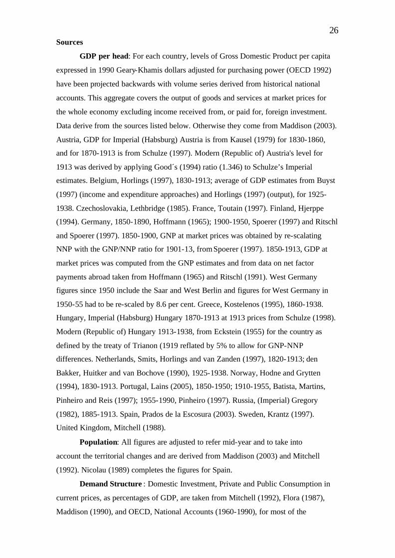
26 Sources

GDP per head: For each country, levels of Gross Domestic Product per capita

expressed in 1990 Geary-Khamis dollars adjusted for purchasing power (OECD 1992)

have been projected backwards with volume series derived from historical national

accounts. This aggregate covers the output of goods and services at market prices for

the whole economy excluding income received from, or paid for, foreign investment. Data derive from the sources listed below. Otherwise they come from Maddison (2003).

Austria, GDP for Imperial (Habsburg) Austria is from Kausel (1979) for 1830-1860,

and for 1870-1913 is from Schulze (1997). Modern (Republic of) Austria's level for

1913 was derived by applying Good´s (1994) ratio (1.346) to Schulze’s Imperial

estimates. Belgium, Horlings (1997), 1830-1913; average of GDP estimates from Buyst

(1997) (income and expenditure approaches) and Horlings (1997) (output), for 1925-

1938. Czechoslovakia, Lethbridge (1985). France, Toutain (1997). Finland, Hjerppe

(1994). Germany, 1850-1890, Hoffmann (1965); 1900-1950, Spoerer (1997) and Ritschl

and Spoerer (1997). 1850-1900, GNP at market prices was obtained by re-scalating

NNP with the GNP/NNP ratio for 1901-13, from Spoerer (1997). 1850-1913, GDP at

market prices was computed from the GNP estimates and from data on net factor

payments abroad taken from Hoffmann (1965) and Ritschl (1991). West Germany

figures since 1950 include the Saar and West Berlin and figures for West Germany in

1950-55 had to be re-scaled by 8.6 per cent. Greece, Kostelenos (1995), 1860-1938.

Hungary, Imperial (Habsburg) Hungary 1870-1913 at 1913 prices from Schulze (1998).

Modern (Republic of) Hungary 1913-1938, from Eckstein (1955) for the country as

defined by the treaty of Trianon (1919 reflated by 5% to allow for GNP-NNP

differences. Netherlands, Smits, Horlings and van Zanden (1997), 1820-1913; den

Bakker, Huitker and van Bochove (1990), 1925-1938. Norway, Hodne and Grytten

(1994), 1830-1913. Portugal, Lains (2005), 1850-1950; 1910-1955, Batista, Martins,

Pinheiro and Reis (1997); 1955-1990, Pinheiro (1997). Russia, (Imperial) Gregory

(1982), 1885-1913. Spain, Prados de la Escosura (2003). Sweden, Krantz (1997).

United Kingdom, Mitchell (1988).

Population: All figures are adjusted to refer mid-year and to take into

account the territorial changes and are derived from Maddison (2003) and Mitchell

(1992). Nicolau (1989) completes the figures for Spain.

Demand Structure : Domestic Investment, Private and Public Consumption in

current prices, as percentages of GDP, are taken from Mitchell (1992), Flora (1987),

Maddison (1990), and OECD, National Accounts (1960-1990), for most of the

27 countries. Spanish figures are from Prados de la Escosura (2003). French figures were

derived from Lévy-Leboyer and Bourguignon (1985) up to 1913, and Carré, Dubois and

Malinvaud (1976) for the remaining years. Figures for Italy are from Ercolani (1978) for

1861-1890 and Rossi, Sorgato and Toniolo (1992) for 1890-1990. In the case of

Portugal, Batista et al. (1997), Pinehiro (1997), and Cartaxo and Da Rosa (1986) were

the references used. For United Kingdom, Feinstein (1972) and Mitchell (1988).

Output Structure: Three major economic sectors are distinguished: Agriculture

(which includes forestry and fishing), Industry (mining, manufacture, construction and

utilities) and services (commerce, transport and communications, banking and private

services, and public administration). Figures are provided as percentages of GDP at

current prices. Most figures are taken from Mitchell (1992), Flora (1987) and OECD,

Historical Statistics. In the case of Spain, Prados de la Escosura (2003). For France,

Toutain (1997) and for Germany prior to World War I, Tilly (1978) and Fremdling

(1988).

Labour Allocation: Distribution of working population by economic sectors.

Three major economic sectors are distinguished: Agriculture (which includes forestry

and fishing), Industry (mining, manufacture, construction and utilities) and services

(commerce, transport and communications, banking and private services, and public

administration). Figures are provided in the form of percentage of total labour force

from Bairoch (1968), Flora (1987), Mitchell (1992) and OECD, Labour Force Statistics,

1969-1989. National figures were completed with Lains (1992) and Nunes (1991) for

Portugal; Toutain (1997) for France; Zamagni (1987) and Vitali (1970) for Italy; Prados

de la Escosura (2003) for Spain.

Foreign Trade : Figures for exports and imports are from Bairoch (1976),

Kuznets (1967), Mitchell (1992) and OECD, National Accounts and Monthly

Statistics of Foreign Trade. For Portugal figures are derived from Nunes, Mata and

Valerio (1989). Spanish figures are from Prados de la Escosura (1988, 2003) and

Tena (1992).

With respect to manufactured export figures, we used Maizels (1963), Batchelor,

Major and Morgan (1980), Baldwin (1958), Spiegelglas (1959), Deustsch and Eckstein

(1961), Lamartine Yates (1959) and Kuznets (1967). Data for particular countries were

completed with Prados de la Escosura (1988, 2003), Tena (1987) for Spain; Davis

(1979), Schlote (1952) for United Kingdom; Levy-Leboyer and Bourguignon (1985)

and Toutain (1977) for France; Eddie (1977) for Hungary; Lains (1992) for Portugal,

and Capanna and Mesori (1940) for Italy.

28 Education: School enrolment refers to population attending primary and

secondary school as a percentage of total population between 5 and 19 years old.

Figures are from Mitchell (1992), Flora (1987), World Bank (1989, 1990 and 1991),

United Nations, Statistical Yearbook, and Demographic Yearbook. As regards Literacy,

it represents the percentage of literate population (those who can read and write) with

respect to total population over 7 years old. In this case, figures are from Flora (1973),

Mitchell (1992) and Hayami and Ruttan (1985). For Italy, Zamagni (1993); for Spain,

Núñez (1992), and for Russia, Mironov (1991).

Urbanization: Population living in towns of 20.000 of inhabitants or more, as a

percentage of total population. Figures are from Flora (1973, 1987).

Demographic Transition: Birth rate and death rates are defined as number of

births and deaths per thousand of population. Infant mortality rate is the number of

deaths per thousand births. Finally, fertility rate refers to the number of births per

thousand of female population. Figures are from Chesnais (1986), Mitchell (1992),

World Bank, Social Indicators of Development (1988, 1989 and 1990), World Tables

(1989, 1990 and 1991), and United Nations, Statistical Yearbook (1987, 1988), and for

Spain Nicolau (1989).

29 TABLE 1

STRUCTURAL CHANGE TESTS: DUMMY VARIABLES D13: value 1 from 1820 to 1913, and 0, thereafter.

D2090: value 0, 1820-1913; 1, 1920-1990.

D38: value 1, 1820-1938; 0, thereafter.

D5090: value 0, 1820-1938; 1, 1950-1990.

D2038: value 0, 1820-1913 and 1950-1990; 1, 1920-1938.

LnY13= D13*lnY

LnY38=D38*LnY

LnY2038=D2038*LnY

LnN13= D13*lnN

LnN38=D38*LnN

LnN2038=D2038*LnN

30 TABLE 2

NORMAL VARIATION IN ECONOMIC STRUCTURE WITH THE LEVEL OF DEVELOPMENT

-Predicted Values at Different Income Levels- US 1990 $ PPP (G-K)

PROCESSES 1000 2000 3000 4000 5000 6000 7000 8000 9000 10000 11000 12000

ACCUMULATION

Investment (% GDP)

SAVING 6.5 11.0 13.7 15.6 17.1 18.3 19.3 20.2 21.0 21.6 22.3 22.8

INVESTMENT 8.3 12.4 14.8 16.5 17.8 18.9 19.8 20.6 21.3 21.9 22.5 23.0

CAPITAL INFLOW 1.8 1.4 1.1 0.9 0.7 0.6 0.5 0.4 0.3 0.3 0.2 0.2

Education (%)

LITERACY 51.1 65.8 74.3 80.4 85.1 89.0 92.2 95.1 97.6 99.8 101.8 103.6

SCHOOLING 31.7 41.1 46.6 50.5 53.6 56.1 58.2 60.0 61.6 63.0 64.3 65.5

RESOURCE ALLOCATION

Demand (% GDP)

PRIVATE CONSUMPTION 87.7 80.1 75.7 72.5 70.0 68.0 66.3 64.9 63.6 62.4 61.4 60.4

GOVT. CONSUMPTION 5.8 8.8 10.6 11.9 12.9 13.7 14.4 14.9 15.5 15.9 16.3 16.7

Production (% GDP)

AGRICULTURE 44.6 33.2 26.4 21.7 18.0 15.0 12.4 10.2 8.3 6.5 5.0 3.5

INDUSTRY 26.4 29.8 31.8 33.2 34.3 35.2 36.0 36.7 37.2 37.8 38.2 38.7

SERVICES 29.0 37.0 41.8 45.1 47.7 49.8 51.6 53.1 54.5 55.7 56.8 57.8

Labour Force (%)

AGRICULTURE 65.7 50.1 41.0 34.6 29.5 25.5 22.0 19.0 16.4 14.0 11.9 9.9

INDUSTRY 21.1 25.9 28.7 30.6 32.2 33.4 34.5 35.4 36.2 36.9 37.6 38.2

SERVICES 13.2 24.0 30.3 34.8 38.3 41.1 43.5 45.6 47.4 49.1 50.5 51.9

Urbanization (%)

URBAN POPULATION 12.6 22.6 28.5 32.7 35.9 38.5 40.8 42.7 44.4 45.9 47.3 48.6

Relative Labour Productivity (%)

AGRICULTURE 68.0 66.2 64.5 62.7 60.9 58.8 56.4 53.7 50.5 46.5 41.6 35.3

Trade (% GDP)

EXPORTS OF GOODS 11.6 15.4 17.6 19.1 20.3 21.4 22.2 22.9 23.6 24.1 24.6 25.1

PRIMARY EXPORTS 11.6 10.9 10.0 9.4 8.9 8.6 8.2 7.9 7.7 7.5 7.3 7.1

MANUFACTURED EXPORTS 0.0 4.5 7.6 9.7 11.4 12.8 14.0 15.0 15.9 16.6 17.3 18.0

IMPORTS OF GOODS 10.9 16.0 18.9 21.1 22.7 24.0 25.2 26.2 27.0 27.8 28.5 29.1

OPENNESS 20.5 31.4 36.5 40.2 43.0 45.4 47.4 49.1 50.6 51.9 53.1 54.2

DEMOGRAPHIC TRANSITION

BIRTH RATE (o/oo) 33.2 27.7 24.5 22.2 20.4 19.0 17.7 16.7 15.7 14.9 14.1 13.5

DEATH RATE (o/oo) 22.2 18.6 16.4 14.9 13.7 12.8 11.9 11.2 10.6 10.0 9.5 9.1

RATE NATURAL INCREASE (o/oo) 11.0 9.1 8.1 7.3 6.7 6.2 5.8 5.5 5.1 4.9 4.6 4.4

FERTILITY 4.6 3.9 3.4 3.1 2.9 2.7 2.5 2.3 2.2 2.1 2.0 1.9

INFANT MORTALITY (o/oo) 186.8 136.8 107.5 86.7 70.6 57.4 46.3 36.6 28.1 20.5 13.6 7.3

NET FERTILITY [FERTILITY*[1-INFMORT/1000]] 3.8 3.3 3.0 2.8 2.6 2.5 2.4 2.2 2.1 2.0 2.0 1.9

31

TABLE 3

NORMAL VARIATION IN GROWTH ELASTICITIES WITH THE LEVEL OF DEVELOPMENT

-Predicted Values at Different Income Levels- US 1990 $ PPP (G-K)

Point Elasticities* Discrete Elasticities** PROCESSES

1000 2000 4000 8000 1000-4000 4000-8000 ACCUMULATION

Investment (% GDP) SAVING 0.632 0.373 INVESTMENT 0.71 0.48 0.36 0.29 0.496 0.320 CAPITAL INFLOW Education (%) LITERACY 0.41 0.32 0.26 0.22 0.327 0.242 SCHOOLING 0.43 0.33 0.27 0.23 0.336 0.249

RESOURCE ALLOCATION Demand (% GDP) PRIVATE CONSUMPTION -0.13 -0.14 -0.15 -0.17 -0.137 -0.160 GOVT. CONSUMPTION 0.80 0.50 0.37 0.30 0.518 0.324 Production (% GDP) AGRICULTURE -0.37 -0.50 -0.76 -01.62 -0.520 -1.089 INDUSTRY 0.23 0.20 0.18 0.16 0.165 0.145 SERVICES 0.40 0.31 0.26 0.22 0.319 0.236 Labour Force (%) AGRICULTURE -0.34 -0.45 -0.65 -1.18 -0.463 -0.840 INDUSTRY 0.33 0.27 0.23 0.20 0.268 0.210 SERVICES 1.18 0.65 0.45 0.34 0.699 0.390 Urbanization (%) URBAN POPULATION 1.15 0.64 0.44 0.34 0.688 0.385 Trade (% GDP) EXPORTS OF GOODS 0.47 0.35 0.28 0.24 0.361 0.262 PRIMARY EXPORTS - - - - -0.152 -0.251 MANUFACTURED EXPORTS - 1.67 0.78 0.50 1.639 0.629 IMPORTS OF GOODS 0.55 0.38 0.28 0.23 0.477 0.312 OPENNESS 0.62 0.41 0.32 0.26 0.486 0.289

DEMOGRAPHIC TRANSITION BIRTH RATE (o/oo) -0.24 -0.29 -0.36 -0.48 -0.290 -0.411 DEATH RATE (o/oo) -0.24 -0.28 -0.36 -0.47 -0.288 -0.412 FERTILITY -0.24 -0.28 -0.35 -0.48 -0.285 -0.431 INFANT MORTALITY (o/oo) -0.39 -0.53 -0.83 -1.97 -0.554 -1.244 NET FERTILITY [FERTILITY*[1-INFMORT/1000]] -0.20 -0.23 -0.27 -0.34 -0.220 -0.348

* Computed as ?

? ?x y

t

tt t

Yx,

ln?

? ?? ? , where ? ? and ? ? are the coefficients for lineal and

quadratic terms of income ( Yt ) in the regresssion, and x t is the predicted value corresponding to the level of income at which the elasticity is being computed.

** Elasticities with respect to GDP per head computed from Table 6 by dividing log differences:

[Ln XT / X0 / Ln YT / Y0]

32

TABLE 4

PRE-WORLD WAR I

NORMAL VARIATION IN ECONOMIC STRUCTURE WITH THE LEVEL OF DEVELOPMENT

-Predicted Values at Different Income Levels- US 1990 $ PPP (G-K)

PROCESSES 1000 1250 1500 1750 2000 2250 2500 2750 3000 3250 3500 4000

ACCUMULATION

Investment (% GDP)

SAVING

INVESTMENT 8.8 9.5 10.1 10.6 11.1 11.4 11.8 12.1 12.4 12.6 12.9 13.3

CAPITAL INFLOW

Education (%)

LITERACY 33.7 43.1 50.7 57.2 62.8 67.7 72.2 76.2 79.8 83.2 86.3 91.9

SCHOOLING 28.2 31.9 34.9 37.4 39.6 41.6 43.3 44.9 46.3 47.6 48.8 51.0

RESOURCE ALLOCATION

Demand (% GDP)

PRIVATE CONSUMPTION 84.7 83.8 83.1 82.5 82.0 81.6 81.2 80.8 80.5 80.2 79.9 79.4

GOVT. CONSUMPTION 6.2 6.4 6.6 6.8 6.9 7.0 7.1 7.2 7.3 7.4 7.5 7.6

Production (% GDP)

AGRICULTURE 47.9 43.9 40.5 37.7 35.3 33.1 31.2 29.5 27.9 26.4 25.1 22.7

INDUSTRY 25.5 26.4 27.2 27.8 28.3 28.9 29.3 29.7 30.0 30.4 30.7 31.2

SERVICES 26.6 29.7 32.3 34.5 36.4 38.0 39.5 40.8 42.1 43.2 44.2 46.1

Labour Force (%)

AGRICULTURE 67.6 61.5 56.4 52.2 48.5 45.2 42.3 39.7 37.3 35.1 33.0 29.3

INDUSTRY 17.4 20.2 22.6 24.5 26.2 27.7 29.0 30.2 31.3 32.3 33.3 35.0

SERVICES 15.0 18.3 21.0 23.3 25.3 27.1 28.7 30.1 31.4 32.6 33.7 35.7

Urbanization (%)

URBAN POPULATION 7.7 12.5 16.4 19.8 22.7 25.3 27.6 29.6 31.5 33.3 34.9 37.8

Relative Labour Productivity (%)

AGRICULTURE 70.8 71.3 71.8 72.3 72.8 73.3 73.8 74.3 74.8 75.4 76.0 77.2

Trade (% GDP)

EXPORTS OF GOODS 9.8 12.5 14.7 16.6 18.3 19.7 21.0 22.2 23.3 24.3 25.2 26.8

PRIMARY EXPORTS 9.8 11.1 11.5 11.8 12.1 12.3 12.5 12.7 13.0 13.1 13.3 13.5

MANUFACTURED EXPORTS 0.0 1.4 3.2 4.8 6.2 7.4 8.5 9.5 10.3 11.2 11.9 13.3

IMPORTS OF GOODS 6.8 9.9 12.5 14.6 16.4 18.1 19.6 20.9 22.1 23.2 24.2 26.1

OPENNESS 16.6 22.4 27.2 31.2 34.7 37.8 40.6 43.1 45.4 47.5 49.4 52.9

DEMOGRAPHIC TRANSITION BIRTH RATE (o/oo) 34.6 33.3 32.1 31.2 30.4 29.6 29.0 28.4 27.8 27.3 26.9 26.1

DEATH RATE (o/oo) 24.1 23.3 22.6 22.0 21.5 21.0 20.6 20.3 19.9 19.6 19.3 18.8

RATE NATURAL INCREASE (o/oo) 10.5 10.0 9.5 9.2 8.9 8.6 8.4 8.1 7.9 7.7 7.6 7.3

FERTILITY 4.7 4.6 4.5 4.4 4.3 4.2 4.2 4.1 4.1 4.0 4.0 3.9

INFANT MORTALITY (o/oo) 194.8 183.4 174.0 166.2 159.3 153.3 147.9 143.0 138.5 134.4 130.6 123.9

NET FERTILITY [FERTILITY*[1-INFMORT/1000]] 3.8 3.7 3.7 3.7 3.6 3.6 3.6 3.5 3.5 3.5 3.5 3.4

33 TABLE 5

PRE-WORLD WAR I

NORMAL VARIATION IN GROWTH ELASTICITIES WITH THE LEVEL OF DEVELOPMENT

-Predicted Values at Different Income Levels- US 1990 $ PPP (G-K)

PROCESSES Point Elasticities* Discrete

Elasticities **

1000 2000 4000 1000-4000 ACCUMULATION

Investment (% GDP) SAVING - INVESTMENT 0.37 0.29 0.24 0.298 CAPITAL INFLOW

Education (%) LITERACY 1.24 0.67 0.46 0.724 SCHOOLING 0.58 0.41 0.32 0.427

RESOURCE ALLOCATION Demand (% GDP) PRIVATE CONSUMPTION -0.05 -0.05 -0.05 -0.047 GOVT. CONSUMPTION 0.17 0.15 0.14 0.147

Production (% GDP) AGRICULTURE -0.38 -0.52 -0.80 -0.539 INDUSTRY 0.18 0.16 0.15 0.146 SERVICES 0.53 0.39 0.31 0.397

Labour Force (%) AGRICULTURE -0.41 -0.57 -0.94 -0.603 INDUSTRY 0.72 0.48 0.36 0.504 SERVICES 1.00 0.59 0.42 0.626

Urbanization (%) URBAN POPULATION 2.82 0.96 0.57 1.148

Trade (% GDP) EXPORTS OF GOODS 1.25 0.67 0.46 0.726 PRIMARY EXPORTS - - - 0.231 MANUFACTURED EXPORTS - 1.64 0.77 1.866 IMPORTS OF GOODS 2.31 0.96 0.60 0.970 OPENNESS 1.58 0.76 0.50 0.836

DEMOGRAPHIC TRANSITION BIRTH RATE (o/oo) -0.18 -0.20 -0.24 -0.203 DEATH RATE (o/oo) -0.16 -0.18 -0.20 -0.179 FERTILITY -0.12 -0.14 -0.15 -0.135 INFANT MORTALITY (o/oo) -0.96 -0.32 -0.41 -0.326 NET FERTILITY [FERTILITY*[1-INFMORT/1000]] -0.09 -0.09 -0.10 -0.080

* Computed as ?

? ?x y

t

tt t

Yx,

ln?

? ?? ? , where ? ? and ? ? are the coefficients for lineal and quadratic terms of

income ( Yt ) in the regression, and x t is the predicted value corresponding to the level of income at which the elasticity is being computed.

** Elasticities with respect to GDP per head computed from Table 8 by dividing log differences: [Ln XT / X0 / Ln YT / Y0 ]

34 APPENDIX

LIST OF DEPENDENT VARIABLES

C/GDP: Private Consumption in current prices as a percentage of GDP.

UGDP: Domestic Investment in current prices as a percentage of GDP.

G/GDP: Public Consumption in current prices as a percentage of GDP.

YAgr/GDP: Output in agriculture in current prices as a percentage of GDP.

YInd/GDP: Output in industry in current prices as a percentage of GDP.

YSer/GDP: Output in services in current prices as a percentage of GDP.

LAgr/L: Labour force in agriculture as a percentage of total labour force.

LInd/L: Labour force in industry as a percentage of total labour force.

LSer/L: Labour force in services as a percentage of total labour force.

Xt/GDP: Exports of goods as a percentage of GDP.

Mt/GDP: Imports of goods as a percentage of GDP.

Open: Exports of goods plus imports of goods as a percentage of GDP.

XInd/GDP: Manufactured exports as a percentage of GDP.

XPrim/GDP: Primary exports as a percentage of GDP.

35

LIST OF EXPLANATORY VARIABLES C: Constant term.

LnY: Log of real per capita, GDP in 1990 US $, PPP.

(LnY)2: Square of the log of real per capita GDP in 1990 US $, PPP.

LnN: Log of population.

(LnN)2: Square of the log of real per capita GDP in 1990 US $, PPP.

INFL: Net imports (imports-exports of goods) as a share of GDP.

D13: Value 1 from 1820 to 1913, and 0, thereafter.

D2038: Value 0 from 1820 to 1913 and from 1950 to 1990, and 1 from 1920 to 1938.

D5090: Value 0 from 1820 to 1938 and 1 from 1950 to 1990.

D2090: Value 0 from 1820 to 1913 and 1 from 1920 to 1990.

D38: Value 1 from 1820 to 1938 and 0, thereafter.

LnY13: D13 * LnY.

LnY203S: D2038 * LnY.

LnY38: D38 * LnY.

TREND: Time trend dummy.

LnN13: D13 * LnN.

LnN38: D38 * LnN.

LnN2038: D2038 * LnN.

LnSize: Log of each country's extension in squared kilometers.

36 LIST OF COUNTRIES (1850-1990) Austria Belgium Czechoslovakia, 1913-1938 Denmark Finland since 1860 France Germany Greece Hungary, 1870-1938 Italy, since 1860 Netherlands Norway, since 1870 Portugal Russia, 1880-1913 Spain Sweden Switzerland, since 1880 UK

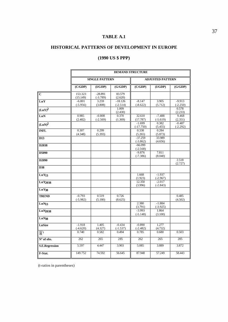
37 TABLE A.1

HISTORICAL PATTERNS OF DEVELOPMENT IN EUROPE

(1990 US $ PPP)

DEMAND STRUCTURE

SINGLE PATTERN ADJUSTED PATTERN

(C/GDP) (I/GDP) (G/GDP) (C/GDP) (I/GDP) (G/GDP)

C

153.323 (15.149)

-28.891 (-3.789)

83.579 (2.620)

LnY -6.801 (-5.956)

3.259 (3.808)

-18.126 (-2.514)

-8.147 (-8.622)

3.905 (5.712)

-9.913 (-2.250)

(LnY)2 1.009 (2.430)

0.578 (2.233)

LnN 0.985 (2.482)

-0.808 (-2.569)

0.370 (1.369)

32.610 (17.787)

-7.488 (-5.619)

9.468 (2.351)

(LnN)2 -1.699 (-17.750)

0.382 (5.455)

-0.487 (-2.292)

INFL 0.307 (4.348)

0.299 (5.393)

0.338 (5.265)

0.284 (5.873)

D13 -37.259 (-3.862)

33.989 (4.656)

D2038 -66.099 (-2.568)

D5090 -9.876 (-7.386)

7.811 (8.040)

D2090 2.518 (2.727)

D38

LnY13 1.668 (1.923)

-1.937 (-2.967)

LnY2038 12.350 (3.996)

-2.017 (-2.843)

LnY38

TREND -0.793 (-5.982)

0.519 (5.180)

0.726 (8.625)

0.485 (4.502)

LnN13 2.380 (3.791)

-1.884 (-3.925)

LnN2038

-3.993 (-5.148)

1.864 (3.100)

LnN38

LnSize -1.918 (-4.620)

1.405 (4.327)

-0.434 (-1.537)

-0.890 (-2.482)

1.277 (4.732)

R 2

0.740 0.582 0.494 0.785 0.680 0.503

Nº of obs. 262 265 285 262 265 285

S.E.Regression

5.597 4.447 3.903 5.085 3.889 3.872

F-Stat. 149.752 74.592 56.645 87.948 57.249 58.443

(t-ratios in parentheses)

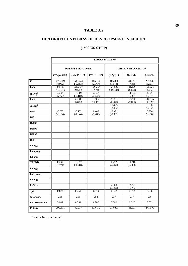
38 TABLE A.2

HISTORICAL PATTERNS OF DEVELOPMENT IN EUROPE

(1990 US $ PPP)

SINGLE PATTERN

OUTPUT STRUCTURE

LABOUR ALLOCATION

(YAgr/GDP) (YInd/GDP) (YSer/GDP) (LAgr/L) (LInd/L) (LSer/L)

C 476.119 (8.962)

-545.224 (-9.653)

165.154 (2.967)

105.368 (1.873)

-342.291 (-7.865)

297.843 (5.361)

LnY -90.407 (-7.201)

126.737 (9.516)

-36.257 (-2.746)

-26.835 (-19.134)

81.886 (8.030)

-58.321 (-5.352)

(LnY)2 4.232 (5.768)

-7.069 (-9.100)

2.837 (3.643)

-4.194 (-6.997)

4.379 (6.807)

LnN 2.304 (5.838)

-1.933 (-4.951)

25.391 (2.281)

3.054 (7.025)

-16.915 (-2.126)

(LnN)2 -1.433 (-2.432)

0.836 (2.002)

INFL -0.272 (-3.354)

-0.172 (-1.944)

0.466 (5.289)

-0.321 (-3.362)

0.254 (3.356)

D13

D2038

D5090

D2090

D38

LnY13

LnY2038

LnY38

TREND 0.239 (1.774)

-0.257 (-1.768)

0.752 (4.260)

-0.716 (-5.858)

LnN13

LnN2038

LnN38

LnSize 2.608 (4.059)

-2.773 (-6.282)

R 2

0.823 0.450 0.679 0.847 0.597 0.836

Nº of obs. 253 253 252 237 237 236

S.E. Regression 5.952 6.299 6.307 7.602 6.017 5.601

F-Stat. 293.871 42.237 133.572 218.891 81.537 241.500

(t-ratios in parentheses)

39 TABLE A.3

HISTORICAL PATTERNS OF DEVELOPMENT IN EUROPE

(1990 US $ 1990)

ADJUSTED PATTERN

OUTPUT STRUCTURE

LABOUR ALLOCATION

(YAgr/GDP) (YInd/GDP) (YSer/GDP) (LAgr/L) (LInd/L) (LSer/L)

C 105.368 (1.873)

LnY -16.309 (-11.992)

23.461 (3.355)

-12.382 (-1.538)

-26.835 (-19.134)

30.260 (3.599)

-3.654 (-2.856)

(LnY)2 -1.058 (-2.522)

1.320 (2.747)

-1.108 (-2.169)

1.237 (12.975)

LnN 31.996 (14.218)

-21.593 (-3.398)

12.731 (1.774)

25.391 (2.281)

-24.006 (-3.375)

-2.072 (-3.888)

(LnN)2 -1.789 (-16.192)

1.357 (4.007)

-0.778 (-2.072)

-1.433 (-2.432)

1.424 (3.804)

INFL -0.380 (-4.711)

0.419 (4.957)

-0.321 (-3.362)

0.157 (1.953)

0.147 (1.965)

D13 24.000 (3.436)

-47.442 (-4.133)

-15.394 (-2.153)

D2038 9.101 (5.662)

D5090 13.616 (5.881)

-7.572 (-3.125)

D2090 -7.770 (-4.700)

8.029 (4.748)

-3.129 (-2.646)

D38

LnY13 -1.937 (-2.852)

3.793 (3.566)

LnY2038 1.895 (1.691)

LnY38

TREND 0.572 (2.981)

-0.892 (-4.263)

0.529 (2.393)

0.752 (4.260)

-1.255 (-6.627)

LnN13 2.014 (3.332)

-2.916 (-3.965)

1.699 (2.224)

1.643 (2.185)

LnN2038 -1.807 (-1.929)

LnN38

LnSize 1.106 (2.479)

2.608 (4.059)

-2.692 (-5.459)

R 2

0.816 0.507 0.709 0.847 0.569 0.823

Nº of obs. 253 277 252 237 236 236

S.E. Regression 6.063 6.171 6.005 7.602 5.924 5.823

F-Stat 140.983 36.541 56.554 218.891 45.350 183.545

(t-ratios in parentheses)

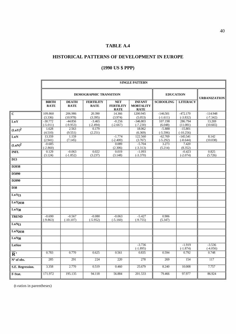
40

TABLE A.4

HISTORICAL PATTERNS OF DEVELOPMENT IN EUROPE

(1990 US $ PPP) SINGLE PATTERN

DEMOGRAPHIC TRANSITION

EDUCATION

URBANIZATION BIRTH

RATE DEATH RATE

FERTILITY RATE

NET FERTILITY

RATE

INFANT MORTALITY

RATE

SCHOOLING LITERACY

C 109.860 (3.336)

206.986 (10.978)

20.390 (3.395)

14.366 (3.974)

1200.945 (5.053)

-146.501 (-1.611)

-472.170 (-3.832)

-114.948 (-7.342)

LnY -30.772 (-5.011)

-44.856 (-9.953)

-3.465 (-2.494)

-0.256 (-2.667)

-346.803 (-7.230)

107.198 (6.048)

286.794 (11.081)

13.269 (10.665)

(LnY)2 1.628 (4.510)

2.563 (9.551)

0.179 (2.251)

18.062 (6.369)

-5.888 (-5.596)

-15.801 (-10.256)

LnN 13.359 (2.941)

1.159 (7.145)

-1.774 (-2.400)

122.560 (3.767)

-62.769 (-5.292)

-145.541 (-8.644)

8.142 (10.038)

(LnN)2 -0.685 (-2.860)

0.089 (2.306)

-5.704 (-3.313)

3.273 (5.214)

7.420 (8.352)

INFL 0.129 (3.124)

-0.063 (-1.852)

0.022 (3.237)

0.019 (3.148)

-1.093 (-3.370)

-0.423 (-2.074)

0.825 (5.726)

D13

D2038

D5090

D2090

D38

LnY13

LnY2038

LnY38

TREND -0.690 (-9.863)

-0.567 (-10.107)

-0.080 (-5.952)

-0.063 (-5.160)

-5.427 (-9.755)

0.906 (5.347)

LnN13

LnN2038

LnN38

LnSize -3.736 (-1.895)

-1.919 (-1.874)

-3.536 (-4.056)

R 2

0.783 0.770 0.625 0.561 0.835 0.594 0.792 0.748

Nº of obs. 285 291 224 220 278 269 154 117

S.E. Regression. 3.358 2.770 0.519 0.460 25.679 8.240 10.008 7.757

F-Stat. 171.972 195.135 94.118 56.884 201.533 79.466 97.977 86.924

(t-ratios in parentheses)

41

TABLE A.5

HISTORICAL PATTERNS OF DEVELOPMENT IN EUROPE

(1990 US $ PPP)

ADJUSTED PATTERN

DEMOGRAPHIC TRANSITION

EDUCATION

URBANIZATION BIRTH

RATE DEATH RATE

FERTILITY RATE

NET FERTILITY

RATE

INFANT MORTALITY

RATE

SCHOOLING LITERACY

C -472.170 (-3.832)

-114.949 (-7.342)

LnY -2.482 (-3.855)

-16.819 (-4.905)

1.852 (21.728)

1.522 (17.884)

-125.464 (-4.259)

95.595 (8.691)

286.794 (11.081)

13.269 (10.665)

(LnY)2 0.998 (4.834)

-0.130 (-14.853)

-0.104 (-12.398)

5.971 (3.427)

-5.452 (-8.025)

-15.801 (-10.256)

LnN 16.392 (14.422)

17.460 (6.032)

-0.099 (-3.349)

-0.058 (-2.109)

161.252 (6.059)

-77.983 (-8.249)

-145.541 (-8.644)

8.142 (10.038)

(LnN)2 -0.850 (-14.045)

-0.914 (-5.966)

-8.227 (-5.906)

4.125 (8.210)

7.420 (8.352)

INFL 0.130 (3.384)

-0.073 (-2.185)

0.014 (2.760)

-1.195 (-4.181)

-0.423 (-2.074)

0.825 (5.727)

D13 1.033 (2.746)

0.130 (2.177)

-45.904 (-3.627)

D2038 -2.565 (-3.125)

21.819 (2.655)

191.984 (2.645)

-2.753 (-2.433)

D5090 -27.751 (-3.776)

-5.553 (-5.612)

-54.512 (-6.044)

D2090 -0.788 (-6.099)

-0.518 (-4.297)

D38

LnY13 -1.231 (-4.436)

-11.662 (-4.619)

5.083.6 (3.356)

LnY2038 -3.148 (-3.123)

-26.688 (-3.008)

LnY38 -3.267 (-3.615)

-0.084 (-5.965)

-0.091 (-7.209)

TREND -0.616 (-5.986)

-0.296 (-3.329)

-0.101 (-5.436)

-0.096 (-5.722)

-2.601 (-3.045)

0.997 (5.955)

LnN13 1.092 (4.385)

11.632 (5.088)

LnN2038

LnN38

LnSize 0.881 (4.480)

-1.009 (-1.720)

-1.919 (-1.874)

-3.537 (-4.056)

R 2

0.813 0.786 0.764 0.675 0.863 0.629 0.792 0.748

Nº. of obs. 285 291 245 220 278 269 154 117

S.E.Regression. 3.115 2.673 0.464 0.396 23.367 7.875 10.008 7.757

F-Stat. 155.819 97.742 132.962 76.682 176.284 57.881 97.977 86.924

(t-ratios in parentheses)

42

TABLE A.6

HISTORICAL PATTERNS OF DEVELOPMENT IN EUROPE

(1990 US $ PPP)

SINGLE PATTERN

EXTERNAL TRADE

(Xt/GDP) (Mt/GDP) OPEN (XInd/GDP) Xprim/GDP

C 117.739 (2.542)

138.837 (2.970)

277.674 (2.970)

-241.242 (-5.521)

125.322 (2.405)

LnY 8.988 (7.556)

8.542 (7.140)

17.084 (7.140)

10.591 (8.939)

19.809 (2.276)

(LnY)2 -1.217 (-2.362)

LnN -24.329 (-2.667)

-27.116 (-2.967)

-54.231 (-2.967)

43.342 (4.900)

-32.507 (-4.050)

(LnN)2 1.187 (2.451)

1.325 (2.733)

2.649 (2.733)

-2.263 (-4.858)

1.557 (3.687)

INFL

0.790 (9.001)

0.580 (3.306)

-0.167 (-2.225)

D13

D2038

D5090

D2090

D38

LnY13

LnY2038

LnY38

TREND -0.517 (-3.423)

-0.475 (-3.141)

-0.950 (-3.141)

-0.581 (-4.097)

LnN13

LnN2038

LnN38

Ln SIZE -3.645 (-6.589)

-3.912 (-6.974)

-7.824 (-6.974)

-2.746 (-5.896)

-2.461 (-5.796)

R 2

0.484 0.599 0.525 0.599 0.477

Nº of obs. 297 295 295 218 216

S.E. Regression 7.530 7.483 14.965 5.331 4.818

F-Stat. 56.544 74.087 55.171 65.963 33.709

(t-ratios in parentheses)

43

TABLE A.7

HISTORICAL PATTERNS OF DEVELOPMENT IN EUROPE

(1990 US $ PPP)

ADJUSTED PATTERN

EXTERNAL TRADE

(Xt/GDP) (Mt/GDP) OPEN (XInd/GDP) Xprim/GDP

C

LnY 10.429 (17.638)

10.664 (17.553)

21.212 (17.568)

-21.431 (-3.059)

37.907 (5.853)

(LnY)2 1.778 (4.235)

-2.139 (-5.566)

LnN -2.192 (-4.356)

-2.325 (-4.559)

-4.682 (-4.586)

17.649 (2.740)

-23.668 (-4.198)

(LnN)2

-0.943 (-2.850)

1.076 (3.657)

INFL

0.864 (10.798)

0.734 (4.588)

-0.210 (-2.904)

D13 21.415 (2.565)

21.997 (2.599)

45.396 (2.684)

-1.553 (-2.149)

15.177 (2.098)

D2038 -7.196 (-5.565)

-3.917 (-3.182)

D5090 -9.654 (-6.517)

-9.852 (-6.572)

18.928 (2.579)

D2090 -19.305 (-6.537)

-3.935 (-3.639)

D38

LnY13 -2.570 (-2.621)

-2.648 (-2.666)

-5.454 (-2.748)

-1.650 (-1.964)

LnY2038 -0.872 (-5.422)

0.648 (2.286)

LnY38

TREND

LnN13

LnN2038

LnN38 2.595 (3.499)

LnSize -3.472 (-8.176)

-3.475 (-8.140)

-6.868 (-8.075)

-3.134 (-7.012)

-2.386 (-5.706)

R 2

0.523 0.625 0.555 0.624 0.502

Nº of obs. 297 295 295 218 216

S.E. Regression 7.239 7.236 14.482 5.162 4.703

F-Stat. 55.134 70.905 53.433 46.110 28.093

(t-ratios in parentheses)