Gerhard Tutz & Gunther Schauberger

Uncertainty as Response Style in Latent Trait Models

Technical Report Number 217, 2018Department of StatisticsUniversity of Munich

http://www.statistik.uni-muenchen.de

Uncertainty as Response Style in Latent TraitModels

Gerhard Tutz & Gunther Schauberger

Ludwig-Maximilians-Universitat Munchen

Akademiestraße 1, 80799 Munchen

September 24, 2018

Abstract

It is well known that the presence of response styles can affect estimates initem response models. Various approaches to account for response styleshave been suggested, in particular the tendency to extreme or middle cat-egories has been included in the modelling of item responses. A responsestyle that has been rarely considered is the noncontingent response style,which occurs if persons have a tendency to respond randomly and non-purposefully, which might also be a consequence of indecision. A modelis proposed that extends the Rasch model and the Partial Credit Modelto account for a response style that accounts for subject-specific uncer-tainty when responding to items. It is demonstrated that ignoring thesubject-specific uncertainty may yield biased estimates of model parame-ters. Uncertainty as well as the underlying trait are linked to explanatoryvariables. The parameterization allows to identify subgroups that differ inresponse style and underlying trait. The modeling approach is illustratedby using data on the confidence of citizens in public institutions.

Keywords: Rasch model; Partial credit model; Rating scales; Response styles;Ordinal data; Heterogeneity, Dispersion; Differential Item Functioning.

1 Introduction

Response styles are a problem in psychological measurement since ignoring theirpresence typically yields biased estimates and can affect the validity of scalescores. Models that explicitly account for response styles and model the hetero-geneity in the population are able to reduce the bias and yield better inference,in particular if response styles are linked to explanatory variables.

1

Various methods for investigating response styles in latent trait theory havebeen proposed. Bolt and Johnson (2009), Johnson and Bolt (2010), Bolt andNewton (2011), and Falk and Cai (2016) use the multi-trait model to investigatethe presence of a response style dimension. Johnson (2003) considered a cumu-lative type model for extreme response styles, Wetzel and Carstensen (2017),Plieninger (2016) and Tutz et al. (2018) proposed partial credit models that ac-count for specific response styles. An alternative strategy for measuring responsestyle is the use of finite mixtures. Eid and Rauber (2000) considered a mixtureof partial credit models. It is assumed that the whole population can be dividedinto disjunctive latent classes. After classes have been identified it is investi-gated if item characteristics differ between classes, potentially revealing differingresponse styles. Finite mixture models for item response data were also consid-ered by Gollwitzer et al. (2005) and Maij-de Meij et al. (2008). Related latentclass approaches were used by Moors (2004), Kankaras and Moors (2009), Moors(2010) and Van Rosmalen et al. (2010).

More recently, tree-based methods to investigate response styles have beenproposed. In tree-based methods one assumes a nested structure, first a decisionabout the direction of the response is modelled and then the strength. Models ofthis type have been considered by Suh and Bolt (2010), De Boeck and Partchev(2012), Thissen-Roe and Thissen (2013), Jeon and De Boeck (2016), Bocken-holt (2012), Khorramdel and von Davier (2014), Plieninger and Meiser (2014),Bockenholt (2017) and Bockenholt and Meiser (2017).

The focus of the present paper is on the noncontingent response style (NCR),which seems to have been neglected in the literature. The noncontingent re-sponse style is found if persons have a tendency to respond to items carelessly,randomly, or nonpurposefully (Van Vaerenbergh and Thomas, 2013; Baumgart-ner and Steenkamp, 2001). Although tree-based methods are strong tools it seemshard to capture this response style by tree-based methods. Given their hierar-chical nature they are more appropriate to model extreme response styles or thepreference for specific categories. Finite mixture model that are in common usetypically fit different item response models in the components without specifyinga specific structure. However, if one does not specify a response style structurein the components it is hard to identify specific response styles after fitting. Fi-nite mixture models that should be mentioned because they do assume a specificstructure in one of the components to account for uncertainty are the so-calledCUB models, which have been propagated in a series of papers by Piccolo (2003),D’Elia and Piccolo (2005), Iannario and Piccolo (2016), Gottard et al. (2016),Tutz et al. (2017), Simone and Tutz (2018). The basic assumption is that thechoice of a response category is determined by a mixture of a distinct preferenceand uncertainty. The latter is represented by a uniform distribution over theresponse categories. But CUB models are designed as regression models withoutassuming repeated measurements, they are not latent trait models, uncertaintyis linked to explanatory variables, and they do not account for subject-specific

2

response styles.The modelling strategy proposed in the following is the explicit modelling of

the noncontingent response style by introducing subject-specific parameters thatare consistent throughout items and might be determined by external explanatoryvariables. The proposed model explicitly aims at modelling the heterogeneity inthe population. We consider in detail extensions of the partial credit model,which contains the binary Rasch model as the most important member.

2 Unobserved Heterogeneity and the Occurrence of Invalid

Parameters

In the following we consider a specific form of unobserved heterogeneity that cancause severe problems in latent trait models. It is of interest because it can beseen as one of the sources of a noncontingent response style and a motivationfor the model that is proposed. For simplicity we consider the binary Raschmodel although the same problems are found in latent trait models with morethan two response categories. The binary Rasch model assumes that the responseYpi ∈ {0, 1} of person p when meeting item i is determined by

P (Ypi = 1) =exp(θp − δi)

1 + exp(θp − δi), p = 1, . . . , P, i = 1, . . . , I.

In achievement tests, θp typically represents the ability of the person and δi thedifficulty of the item. In questionnaires θp may represent the attitude and δi anitem-specific threshold on the latent scale. In both cases it is assumed that theparameters are on the same latent scale. For the identification of problems thatmay arise when using the Rasch model it is instructive to consider the derivationof the model from the assumption of latent random variables. When person pmeets item i one assumes:

• The ability or attitude is determined by the continuous random variable Y ∗pi =

θp + σεpi, where θp is a fixed parameter linked to the person, εpi is a randomvariable that represents the variability of the response and σ is a dispersionparameter.

• The link between the unobserved variable Y ∗pi and the observed response is given

byYpi = 1 if Y ∗

pi ≥ δi, (1)

which means that one observes Ypi = 1 if the latent variable is larger than theitem-specific threshold δi.

If one assumes that the noise variable εpi has the logistic distribution functionF (η) = exp(η)/(1 + exp(η)), it is straightforward to derive the model

P (Ypi = 1) =exp((θp − δi)/σ)

1 + exp((θp − δi)/σ)), p = 1, . . . , P, i = 1, . . . , I.

3

Since the parameters in this representation are not identifiable, constraints onthe parameters are needed. Typically one uses the scale constraint σ = 1 anda location constraint by choosing a fixed value for one of the parameters, forexample, θ1 = 0 or δ1 = 0. Then the model is equivalent to the Rasch modelwith a location constraint, which is always needed and is assumed to be fixed inthe following.

The derivation uses implicitly that the dispersion parameter σ is the samefor all persons. However, this is a strong assumption that does not have to hold.Let us assume more generally that the latent variable is given by Y ∗

pi = θp +σpεpiwith person-specific dispersion σp. To keep things simple let us first consider thecase where the dispersion takes only two values, depending on a binary trait likegender or age group (young/old). This can be represented by σp = exp(xpγ),where xp is a group indicator with values xp ∈ {0, 1}. Then one obtains

σp =

{exp(γ) if xp = 11 if xp = 0.

If one derives the observed response in the same way as previously as a di-chotomized version of latent variables one obtains different parameters for thetwo groups. More concrete, one obtains

log

(P (Ypi = 1)

P (Ypi = 0)

)= θp − δi, in the group xp = 0

log

(P (Ypi = 1)

P (Ypi = 0)

)=θpeγ− δieγ, in the group xp = 1.

This entails peculiar effects if one wants to compare parameters. Actually onehas two Rasch models, one that holds in the subpopulation xp = 0 and one inthe subpopulation xp = 1. Formally these can be given by

log

(P (Ypi = 1)

P (Ypi = 0)

)= θ(s)p − δ(s)i , s = 0, 1, (2)

with s = 0 representing xp = 0 and s = 1 representing xp = 1. In the groupxp = 0 one has the original parameters

θ(0)p = θp, p = 1, . . . , P, δ(0)i = δi, i = 1, . . . , I,

whereas in the group xp = 1 one has the parameters

θ(1)p =θpeγ, p = 1, . . . , P, δ

(1)i =

δieγ, i = 1, . . . , I.

It is essential that in both subpopulations simple Rasch models hold. However,comparison of parameters between groups may be strongly misleading. For illus-tration, let xp refer to gender with xp = 1 coding females and xp = 0 males. Let

4

us consider two persons, one female with parameter θf , one male with parameterθm, which have the same strength parameter, that is, θf = θm. If one comparesthe Rasch model parameters of the two persons one obtains

θ(0)m

θ(1)f

=θmθfeγ = eγ.

That means, if γ > 0, although the underlying abilities are the same (θf = θm),the comparison of the Rasch model parameters measured by the Rasch modelparameters θ

(s)p indicates that the ability of the male person is larger than the

ability of the female person. The reason is that the female person is confrontedwith ”simpler” items δi/e

γ than the male persons. Consequently, the ability offemales measured in terms of the Rasch model parameters is considered to belower for females.

It should be noted that the Rasch model does not hold in the total population.However, it holds in each subpopulation and can be legitimately fitted withinsubpopulations. But parameters (and parameter estimates) can not be comparedsince parameters in each subpopulation are scaled by using the scale constraintσ = 1 in each subpopulation.

Even if one does not want to compare parameter estimates it is obvious thatone runs into problems if one ignores heterogeneity and fits a simple Rasch modelto the total population. The heterogeneity of the person parameters is less severebecause although the persons come from different subpopulations each person hashis/her own parameter. However, estimates of item parameters tend to be biasedbecause persons from different subpopulations meet items with different difficultyparameters. For males the difficulties are δi and for females δi/e

γ, which may beseen as a specific form of differential item functioning, which will be discussedlater.

Similar problems with unobserved heterogeneity have been found for binaryand ordinal regression models, Allison (1999) showed that misleading parameterestimates can occur if one fits a binary logit model in separate groups. Somemethods to correct parameter estimates in regression were considered by Williams(2009), Mood (2010), Karlson et al. (2012), Breen et al. (2014), and Tutz (2018).

3 Heterogeneity and Response Styles

In the following we consider models that are able to avoid the occurrence of biasedestimates caused by unobserved heterogeneity. We will consider the family ofRasch models represented by the partial credit model. First we briefly considerthe partial credit model.

5

3.1 The Partial Credit Model

Let Ypi ∈ {0, 1, . . . , k}, p = 1, . . . , P , i = 1, . . . , I denote the ordinal response ofperson p on item i. The partial credit model (PCM) assumes for the probabilities

P (Ypi = r) =exp(

∑rl=1 θp − δil)∑k

s=0 exp(∑s

l=1 θp − δil), r = 1, . . . , k,

where θp is the person parameter and (δi1, . . . , δik) are the item parameters ofitem i. For notational convenience the definition of the model implicitly uses∑0

k=1 θp − δik = 0. With this convention an alternative form is given by

P (Ypi = r) =exp(rθp −

∑rk=1 δik)∑k

s=0 exp(∑s

k=1 θp − δik).

The PCM was proposed by Masters (1982), see also Masters and Wright (1984).The defining property of the partial credit model is seen if one considers

adjacent categories. The resulting presentation

log

(P (Ypi = r)

P (Ypi = r − 1)

)= θp − δir, r = 1, . . . , k

shows that the model is locally (given response categories r − 1, r) a binaryRasch model with person parameter θp and item difficulty δir. It is immediatelyseen that for θp = δir the probabilities of adjacent categories are equal, that is,P (Ypi = r) = P (Ypi = r − 1).

3.2 An Extended Partial Credit Model

The extended version of the partial credit model that is proposed has the form

P (Ypi = r) =exp(

∑rl=1 e

αp(θp − δil))∑ks=0 exp(

∑sl=1 e

αp(θp − δil)), r = 1, . . . , k. (3)

Thus, the usual predictor in the PCM, ηpir = θp−δir, which distinguishes betweencategory r − 1 and r, is replaced by the more general predictor

ηpir = eαp(θp − δir), r = 1, . . . , k,

which contains the additional subject-specific parameter αp. As is discussed inthe following, the parameter αp can be seen as a subject-specific response styleparameter, which describes a tendency to a specific response pattern.

6

Interpretation of Subject-Specific Parameters

Let us start with the simplest case of a binary response (k = 1). Then it is easilyseen that the following holds.

If αp = 0 for all p one obtains the binary Rasch model.

If αp > 0 the person p is a strong discriminator, he/she has a distinctpreference for specific categories. For αp →∞ one obtains P (Ypi = 1) = 1if θp > δi1, and P (Ypi = 0) = 1 if θp < δi1.

If αp < 0 the person p is a weak discriminator, For αp → −∞ one obtainsP (Ypi = 1) = 0.5 for all abilities/attitudes θp. The person shows a non-contingent response style (NCR), which means he/she has a tendency torespond to items randomly, or nonpurposefully.

In the general PCM one has to distinguish between two cases, ordered thresh-olds and un-ordered thresholds. In the case of ordered thresholds (δir ≤ δi,r+1)one obtains the following:

If αp = 0 for all p one obtains the traditional PCM.

For αp →∞ one obtains for a person with θp ∈ (δir, δi,r+1) the probabilityP (Ypi = r) = 1, one observes a distinct response, the person knows exactlywhich category he/she prefers. The property holds for all k if one definesin addition δi0 = −∞, δi,k+1 =∞.

For αp → −∞ one obtains P (Ypi = r) = 1/(k+ 1) for all abilities/attitudesθp. The person’s response has a discrete uniform distribution over theresponse categories, which means simple guessing.

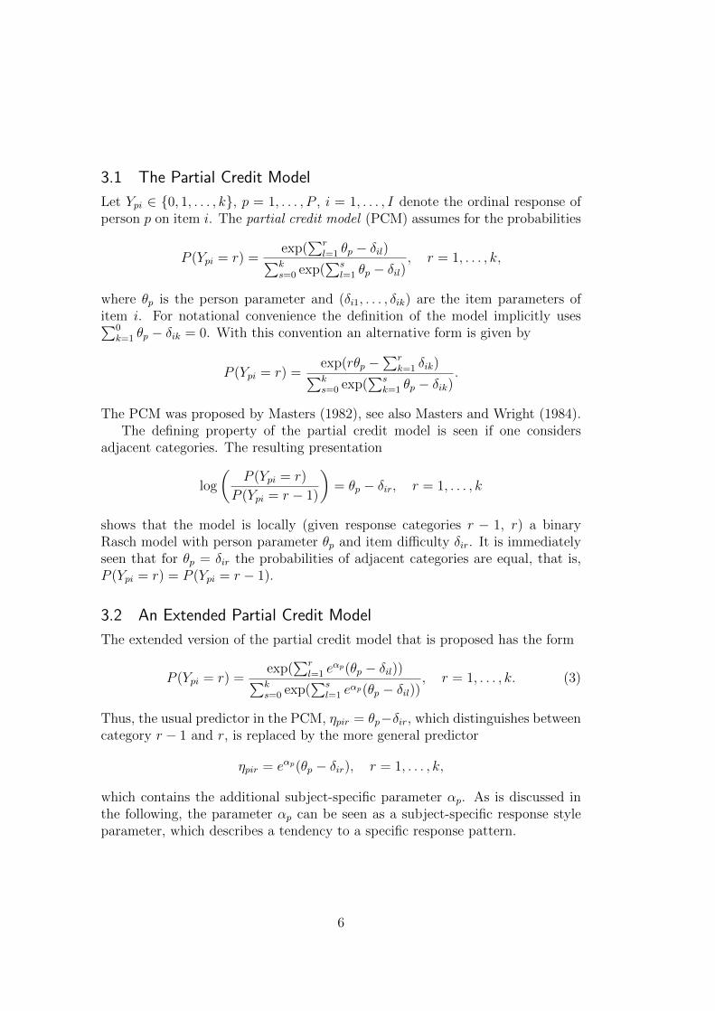
For illustration, the impact of the parameter αp is visualized in Figure 1. Itshows the response probabilities for a PCM with four categories for five differentvalues of αp. For αp = 0 one obtains the response probabilities given in the mid-dle, which represent the response probabilities for the traditional PCM withoutsubject-specific heterogeneity. It is seen that for decreasing αp one comes closerto a uniform distribution across categories, whatever the parameter θp is, for in-creasing αp the preference for categories becomes very distinct depending on thevalue of θp. The chosen parameters are rather large/small so that the impactbecomes obvious.

In the case of three response categories (k = 2), which are considered forsimplicity, and reverse thresholds δi2 < δi1 one obtains the following behaviour.

For αp →∞ the probabilities are given by:

For all persons one obtains P (Ypi = 1) = 0, that is, the middle category isnever chosen.

7

αp = − 4 αp = − 2 αp = 0 αp = 2 αp = 4

−2 0 2 −2 0 2 −2 0 2 −2 0 2 −2 0 2

0.00

0.25

0.50

0.75

1.00

θp

P(Y

pi=

r)

Category

0

1

2

3

Figure 1: Response probabilities in an extended PCM for four values of αp(ordered thresholds).

For person θp < δi2 one obtains P (Ypi = 0) = 1.

For person θp > δi1 one obtains P (Ypi = 2) = 1.

Thus the inverse structure of thresholds yields a more distinct avoidance of themiddle category than the traditional PCM.

For αp → −∞ one obtains again P (Ypi = r) = 1/(k + 1)) for all abili-ties/attitudes θp. The person has a discrete uniform distribution over theresponse category, which means simple guessing.

As has been demonstrated the parameter αp can be seen as modelling thesubject-specific decisiveness or discriminatory power. For large αp the personhas distinct preferences, for small αp the person tends to a choose one of theresponse categories at random which can be seen as noncontingent response styleor indecision. Since it is not possible to determine if indecisiveness or carelessnessis the reason we will, more generally, refer to the subject-specific effect eαp asuncertainty effect. Although the used terminology primarily refers to attitudemeasurement or personality questionnaires uncertainty may also come into playin achievement tests. The uncertainty may refer to a nonpurposeful responserepresenting a person’s ability to work concentrated or distractedly. Withoutspecifying the specific source we consider the term eαp as representing uncertaintyand call the extended model (3) the uncertainty partial credit model (UPCM).

The uncertainty can also explain the occurrence of response patterns thatare unlikely in a unidimensional model in which uncertainty is ignored. Theresponses of a person with high uncertainty is hardly predictable, since he/sheshows random behaviour. Therefore response patterns might occur that appear

8

strange in a unidimensional model that does not account for heterogeneity ofuncertainty.

It should be noted that the response style parameter αp is strongly linkedto the unobvserved heterogeneity considered in Section 2. In the special case ofbinary responses (k = 1) the parameter e−αp in the extended model representsthe unobserved dispersion σp in the latent variable Y ∗

pi = θp+σpεpi With σp = eγp

model, one has γp = −αp. This interpretation is also possible in the general PCM.If one derives the PCM from latent variables locally (given categories r − 1, r)the same reasoning applies as for the binary Rasch model. While eγp representsthe distinctiveness of the response e−γp represents the uncertainty of person p.

Differential Item Functioning

Differential item functioning (DIF) is the well known phenomenon that the prob-ability of a correct response among equally able persons differs in subgroups. Inparticular, the difficulty of an item may depend on the membership to a racial,ethnic or gender subgroup. Then the performance of a group can be lower be-cause these items are related to specific knowledge that is less present in thisgroup. The effect is measurement bias and possibly discrimination. More gen-erally, including ordinal and nominal responses, DIF is present if the responseprobabilities among persons with equal trait differ in subgroups. Various formsof differential item functioning have been considered in the literature, see Magiset al. (2010) for an instructive overview of DIF detection methods.

Differential item functioning usually aims at identifying those items that havedifferent difficulties in differing subgroups. It is typically assumed that just someof the available items show this property. This is different in the case consideredhere when persons have varying uncertainty represented in the factor eαp . Ifthe parameter αp is linked to a binary variable like gender one obtains that theeffective parameters of all all items are modified in one subgroup. Similar as inSection 2 let us consider the binary model and let αp = α if xp = 1 and αp = 0if xp = 0. Then the ’effective’ person and item parameters (eαpθp and eαpδi) ingroup xp = 0 are

θ1, . . . , θP δ1, . . . , δI ,

and in group xp = 1eαθ1, . . . , e

αθP eαδ1, . . . , eαδI .

Thus, even when the underlying abilities θp are the same in both groups theprobability of a correct response differs in the groups, which corresponds to thegeneral definition of DIF that the probability of a correct response among equallyable persons differs in subgroups. Nevertheless, it should be seen as a specificform of DIF, which could be called uniform DIF across items.

One further consequence of the modification of person and item parametersis the reduced possibility of comparing item difficulties. If persons have different

9

response styles, that is, different parameters αp, the person parameters θp cannotbe compared directly. Only for persons p and p, which have the same slopeparameter (αp = αp), the log-odds can be compared directly by

P (Ypi = r)/P (Ypi = r − 1)

P (Ypi = r)/P (Ypi = r − 1)= eθp−θp .

The Generalized Partial Credit Model

It is noteworthy that the extended partial credit model considered here differsfrom the generalized partial credit model as considered by Muraki (1992), Muraki(1997). It assumes

log

(P (Ypi = r)

P (Ypi = r − 1)

)= ai(θp − δir), r = 1, . . . , k,

which includes an item-specific slope parameter ai, not a subject-specific parame-ter. In the generalized partial credit model the items have differing discriminatorypower. In contrast the uncertainty partial credit model considered here allows asubject-specific uncertainty parameter, which means that discriminatory powervaries across persons.

3.3 Including Subject-Specific Characteristics

In the extended PCM each person has its own response style parameter αp, whichyields a large number of parameters. Thus, for estimation it is useful to assumethat they are random effects. In the light of differential item functioning itis of special interest to investigate if response styles (or equivalently dispersionheterogeneity) is determined by subject-specific covariates. To this end we letthe response style parameter depend on a vector of subject-specific covariates xpin the form

αp = αp0 + xTpα,

and assume that αp0 follows the normal distribution IN(0, σ2). In the same wayone can include explanatory variables for the trait parameter by using

θp = θp0 + xTp ξ.

Thus the general uncertainty partial credit model (UPCM) we consider is

P (Ypi = r) =exp(

∑rl=1 e

αp0+xTp α(θp0 + xTp ξ − δil))∑k

s=0 exp(∑s

l=1 eαp0+xT

p α(θp0 + xTp ξ − δil)), r = 1, . . . , k.

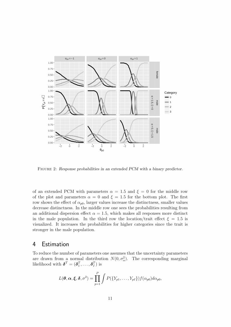
Figure 2 shows the resulting response probabilities if a binary predictor (male:xp = 1, female: xp = 0) is included in the location part and the dispersion part

10

αp0 = − 1 αp0 = 0 αp0 = 1

female

α=

1.5, ξ=

0

male

α=

0, ξ=

1.5

male

−2 0 2 −2 0 2 −2 0 2

0.00

0.25

0.50

0.75

1.00

0.00

0.25

0.50

0.75

1.00

0.00

0.25

0.50

0.75

1.00

θp0

P(Y

pi=

r)

Category

0

1

2

3

Figure 2: Response probabilities in an extended PCM with a binary predictor.

of an extended PCM with parameters α = 1.5 and ξ = 0 for the middle rowof the plot and parameters α = 0 and ξ = 1.5 for the bottom plot. The firstrow shows the effect of αp0, larger values increase the distinctness, smaller valuesdecrease distinctness. In the middle row one sees the probabilities resulting froman additional dispersion effect α = 1.5, which makes all responses more distinctin the male population. In the third row the location/trait effect ξ = 1.5 isvisualized. It increases the probabilities for higher categories since the trait isstronger in the male population.

4 Estimation

To reduce the number of parameters one assumes that the uncertainty parametersare drawn from a normal distribution N(0, σ2

α). The corresponding marginallikelihood with δT = (δT1 , . . . , δ

TI ) is

L(θ,α, ξ, δ, σ2) =P∏

p=1

∫P ({Yp1, . . . , YpI})f(αp0)dαp0,

11

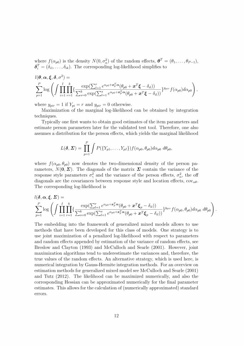
where f(αp0) is the density N(0, σ2α) of the random effects, θT = (θ1, . . . , θP−1),

δTi = (δi1, . . . , δik). The corresponding log-likelihood simplifies to

l(θ,α, ξ, δ, σ2) =

P∑

p=1

log

(∫ I∏

i=1

k∏

r=1

{ exp(∑r

l=1 eαp0+xT

p α(θp0 + xTξ − δil))∑ks=0 exp(

∑sl=1 e

αp0+xTp α(θp0 + xTξ − δil))

}ypirf(αp0)dαp0

),

where ypir = 1 if Ypi = r and ypir = 0 otherwise.Maximization of the marginal log-likelihood can be obtained by integration

techniques.Typically one first wants to obtain good estimates of the item parameters and

estimate person parameters later for the validated test tool. Therefore, one alsoassumes a distribution for the person effects, which yields the marginal likelihood

L(δ,Σ) =P∏

p=1

∫P ({Yp1, . . . , YpI})f(αp0, θp0)dαp0 dθp0,

where f(αp0, θp0) now denotes the two-dimensional density of the person pa-rameters, N(0,Σ). The diagonals of the matrix Σ contain the variance of theresponse style parameters σ2

γ and the variance of the person effects, σ2α, the off

diagonals are the covariances between response style and location effects, covαθ.The corresponding log-likelihood is

l(δ,α, ξ,Σ ) =

P∑

p=1

log

(∫ I∏

i=1

k∏

r=1

{ exp(∑r

l=1 eαp0+xT

p α(θp0 + xTξp − δil))∑ks=0 exp(

∑sl=1 e

αp0+xTp α(θp0 + xTξp − δil))

}ypirf(αp0, θp0)dαp0 dθp0

).

The embedding into the framework of generalized mixed models allows to usemethods that have been developed for this class of models. One strategy is touse joint maximization of a penalized log-likelihood with respect to parametersand random effects appended by estimation of the variance of random effects, seeBreslow and Clayton (1993) and McCulloch and Searle (2001). However, jointmaximization algorithms tend to underestimate the variances and, therefore, thetrue values of the random effects. An alternative strategy, which is used here, isnumerical integration by Gauss-Hermite integration methods. For an overview onestimation methods for generalized mixed model see McCulloch and Searle (2001)and Tutz (2012). The likelihood can be maximized numerically, and also thecorresponding Hessian can be approximated numerically for the final parameterestimates. This allows for the calculation of (numerically approximated) standarderrors.

12

5 Simulations

We conducted a small simulation study to evaluate the performance of the methodand the possible consequences of ignoring the response style. We used n = 300observations on I = 10 items with each item having k = 5 categories. Thedata were simulated under the assumption that the uncertainty partial creditmodel (UPCM) holds. As explanatory variables we used one binary variableand one continuous variables drawn from a standard normal distribution. Wefix the respective effects of the explanatory variables to ξT = (0.2,−0.1) for thetrait effects and αT = (−0.2, 0) for the response style effects. Furthermore, thecovariance matrix of the random effects was fixed to

Σ =

(1 0.1

0.1 0.5

).

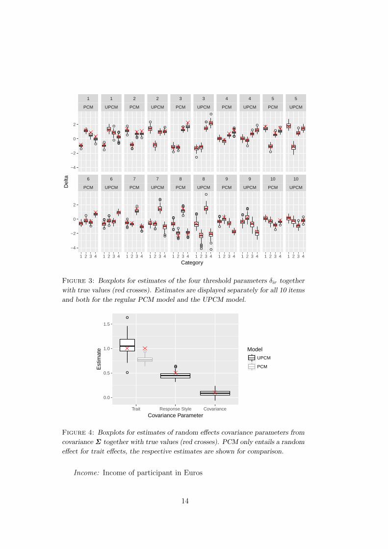
The simulation was conducted with 100 replications. Figure 3 compares the esti-mates of the item parameters of a regular PCM to the item parameter estimatesobtained for the UPCM. The boxplots show the respective estimates together withthe true values, separately for each item and separately for PCM and UPCM.True values are highlighted by (red) crosses. It can be seen, that in contrast tothe UPCM, the regular PCM estimates are biased.

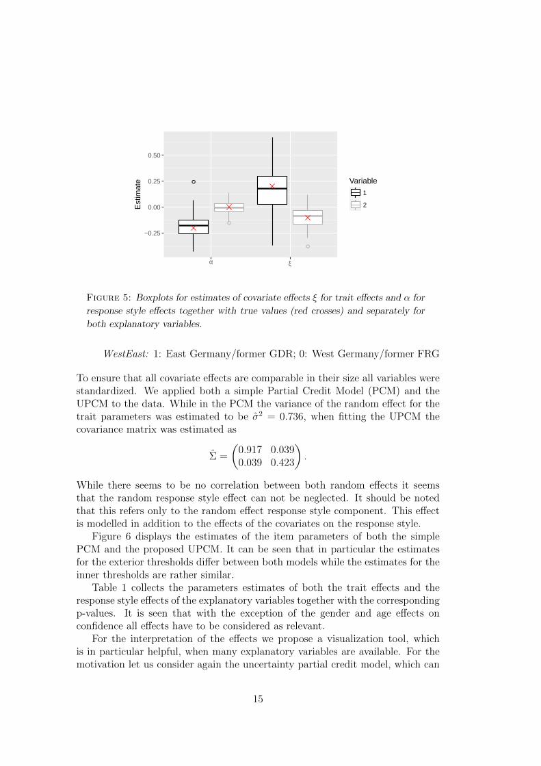
Figure 4 displays the estimates of the random effects covariance matrix Σ .Again the estimates can be compared to estimates from the regular PCM, howeverobviously the PCM only provides estimates for the random effect of the trait.While the PCM clearly underestimates the variance of the trait effects, the UPCMestimates all parameters reasonably well. Figure 5 displays the estimates of allcovariate effects, both for trait and response style effects. All effects are estimatedrather well by the UPCM model.

6 An Application

For illustration, we consider data from the ALLBUS, the general survey of so-cial science carried out by the German institute GESIS (http://www.gesis.org/allbus). The data contain the answers of 2535 respondents from the ques-tionnaire in 2012. In particular, we consider 8 items that refer to the degree ofconfidence the participants have in public institutions and organizations. Theseinstitutions are the federal court, the Bundestag (parliament), the justice system,TV, press, government, police and political parties. The items are measured ona scale from 1 (no confidence at all) to 7 (excessive confidence). As explanatoryvariables for the trait and for the response style effects we used the followingperson characteristics:

Age: Age of participant in years

Gender: 0: male; 1: female

13

●

●

●

●

●

●

●

●

●●●

●●●

●

●

●●

●

●

●

●

●

●●

●● ●

●●

●

●

●●

●

●

●●

●●

●●

●●

●●

●

●●

●●

●

●

●●●

●

●

●●

●●●

●

●●

●

●●●

●●●

●

●

●

●

●●●

●●●

●

●●

●

●

●

●

●●

●●●

●

●

●

●

●

●

●

●

●

6

PCM

6

UPCM

7

PCM

7

UPCM

8

PCM

8

UPCM

9

PCM

9

UPCM

10

PCM

10

UPCM

1

PCM

1

UPCM

2

PCM

2

UPCM

3

PCM

3

UPCM

4

PCM

4

UPCM

5

PCM

5

UPCM

1 2 3 4 1 2 3 4 1 2 3 4 1 2 3 4 1 2 3 4 1 2 3 4 1 2 3 4 1 2 3 4 1 2 3 4 1 2 3 4

−4

−2

0

2

−4

−2

0

2

Category

Del

ta

Figure 3: Boxplots for estimates of the four threshold parameters δir together

with true values (red crosses). Estimates are displayed separately for all 10 items

and both for the regular PCM model and the UPCM model.

●

●

●

●●

0.0

0.5

1.0

1.5

Trait Response Style Covariance

Covariance Parameter

Est

imat

e Model

UPCM

PCM

Figure 4: Boxplots for estimates of random effects covariance parameters from

covariance Σ together with true values (red crosses). PCM only entails a random

effect for trait effects, the respective estimates are shown for comparison.

Income: Income of participant in Euros

14

●

●

●

−0.25

0.00

0.25

0.50

α ξ

Est

imat

e Variable

1

2

Figure 5: Boxplots for estimates of covariate effects ξ for trait effects and α for

response style effects together with true values (red crosses) and separately for

both explanatory variables.

WestEast: 1: East Germany/former GDR; 0: West Germany/former FRG

To ensure that all covariate effects are comparable in their size all variables werestandardized. We applied both a simple Partial Credit Model (PCM) and theUPCM to the data. While in the PCM the variance of the random effect for thetrait parameters was estimated to be σ2 = 0.736, when fitting the UPCM thecovariance matrix was estimated as

Σ =

(0.917 0.0390.039 0.423

).

While there seems to be no correlation between both random effects it seemsthat the random response style effect can not be neglected. It should be notedthat this refers only to the random effect response style component. This effectis modelled in addition to the effects of the covariates on the response style.

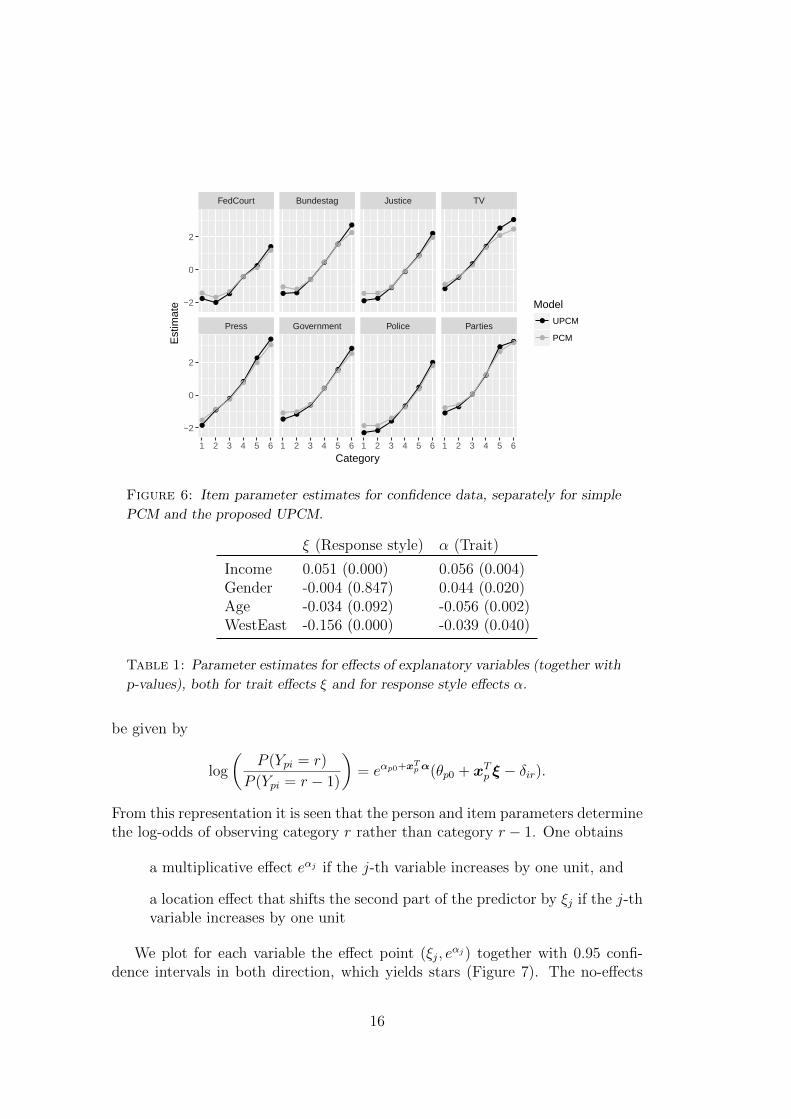
Figure 6 displays the estimates of the item parameters of both the simplePCM and the proposed UPCM. It can be seen that in particular the estimatesfor the exterior thresholds differ between both models while the estimates for theinner thresholds are rather similar.

Table 1 collects the parameters estimates of both the trait effects and theresponse style effects of the explanatory variables together with the correspondingp-values. It is seen that with the exception of the gender and age effects onconfidence all effects have to be considered as relevant.

For the interpretation of the effects we propose a visualization tool, whichis in particular helpful, when many explanatory variables are available. For themotivation let us consider again the uncertainty partial credit model, which can

15

●●

●

●

●

●

●●

●

●

●

●

●

●

●

●

●

●

●

●

●

●

●

●

● ●

●

●

●

●

● ●

●

●

●

●

●●

●

●

●

●

● ●

●

●

●

●

● ●

●

●

●

●

● ●●

●

●

●

● ●

●

●

●

●

● ●

●

●

●

●

●

●

●

●

●

●

●

●

●

●

●●

●●

●

●

●●

●●

●

●

●

●

Press Government Police Parties

FedCourt Bundestag Justice TV

1 2 3 4 5 6 1 2 3 4 5 6 1 2 3 4 5 6 1 2 3 4 5 6

−2

0

2

−2

0

2

Category

Est

imat

e Model●

●

UPCM

PCM

Figure 6: Item parameter estimates for confidence data, separately for simple

PCM and the proposed UPCM.

ξ (Response style) α (Trait)

Income 0.051 (0.000) 0.056 (0.004)Gender -0.004 (0.847) 0.044 (0.020)Age -0.034 (0.092) -0.056 (0.002)WestEast -0.156 (0.000) -0.039 (0.040)

Table 1: Parameter estimates for effects of explanatory variables (together with

p-values), both for trait effects ξ and for response style effects α.

be given by

log

(P (Ypi = r)

P (Ypi = r − 1)

)= eαp0+xT

p α(θp0 + xTp ξ − δir).

From this representation it is seen that the person and item parameters determinethe log-odds of observing category r rather than category r − 1. One obtains

a multiplicative effect eαj if the j-th variable increases by one unit, and

a location effect that shifts the second part of the predictor by ξj if the j-thvariable increases by one unit

We plot for each variable the effect point (ξj, eαj) together with 0.95 confi-

dence intervals in both direction, which yields stars (Figure 7). The no-effects

16

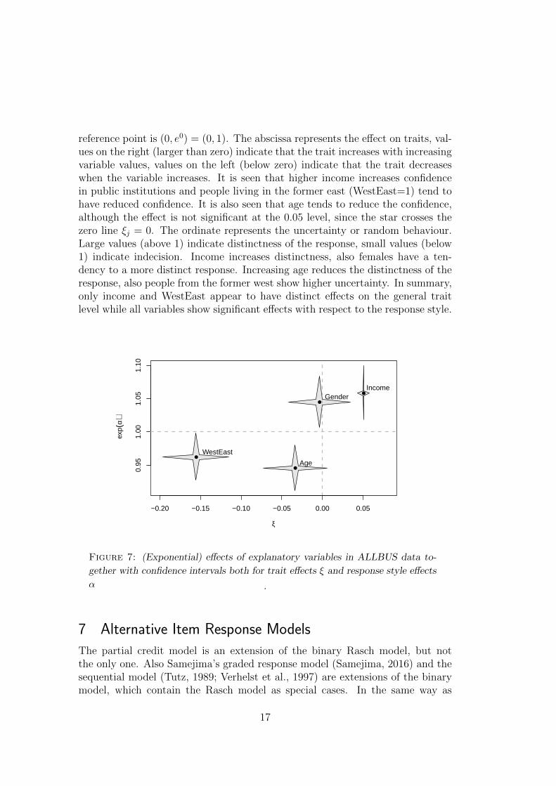
reference point is (0, e0) = (0, 1). The abscissa represents the effect on traits, val-ues on the right (larger than zero) indicate that the trait increases with increasingvariable values, values on the left (below zero) indicate that the trait decreaseswhen the variable increases. It is seen that higher income increases confidencein public institutions and people living in the former east (WestEast=1) tend tohave reduced confidence. It is also seen that age tends to reduce the confidence,although the effect is not significant at the 0.05 level, since the star crosses thezero line ξj = 0. The ordinate represents the uncertainty or random behaviour.Large values (above 1) indicate distinctness of the response, small values (below1) indicate indecision. Income increases distinctness, also females have a ten-dency to a more distinct response. Increasing age reduces the distinctness of theresponse, also people from the former west show higher uncertainty. In summary,only income and WestEast appear to have distinct effects on the general traitlevel while all variables show significant effects with respect to the response style.

●

●

●

●

−0.20 −0.15 −0.10 −0.05 0.00 0.05

0.95

1.00

1.05

1.10

ξ

exp(

α)

●

●

●

●

IncomeGender

Age

WestEast

Figure 7: (Exponential) effects of explanatory variables in ALLBUS data to-

gether with confidence intervals both for trait effects ξ and response style effects

α .

7 Alternative Item Response Models

The partial credit model is an extension of the binary Rasch model, but notthe only one. Also Samejima’s graded response model (Samejima, 2016) and thesequential model (Tutz, 1989; Verhelst et al., 1997) are extensions of the binarymodel, which contain the Rasch model as special cases. In the same way as

17

the partial credit model these models can be extended to contain an additionalsubject-specific uncertainty component. It is less interesting in the sequentialmodel, which assumes a step wise solving of items, but is sensible in the case ofthe graded response model, which can be derived from an underlying latent traitand works well in personality questionnaires and attitude scales. The gradedresponse model has the form

P (Ypi ≥ r) = F (θp − δir), r = 1, . . . , k,

where F (.) again is a cumulative distribution function, typically chosen as thelogistic function. The extended version assumes for the probabilities

P (Ypi ≥ r) = F (eαp(θp − δir)), r = 1, . . . , k, (4)

with eαp representing the subject-specific factor. However, some caution is war-ranted when interpreting the subject-specific term. It differs from the correspond-ing term in the partial credit model. The way the subject-specific term modifiesthe response probabilities is seen best when looking at the extreme cases. Oneobtains the following properties.

For αp = 0 one obtains the traditional graded response model.

For αp →∞ one obtains for a person with θp ∈ (δir, δi,r+1) the probabilityP (Ypi = r) = 1, that means a person knows exactly what he/she wants.

For αp → −∞ one obtains P (Ypi = 0) = P (Ypi = k) = 0.5.

In particular the last case (αp → −∞) shows that the subject-specific termhas a different meaning in the graded response model. Persons with αp → −∞choose one of the extreme categories, which means they show what is called anextreme response style (ERS). Thus when going through the continuum betweenαp = −∞ to αp =∞

one covers the continuum between an extreme response style and a distinctresponse.

For the partial credit model with a subject-specific term

one covers the continuum between a uniform distribution, which meansuncertainty, and a distinct response.

The difference in interpretation is caused by the specific property of the partialcredit model that modification of the local responses (given Y ∈ {r − 1, r})modifies automatically all the other response probabilities. The extended gradedresponse model is in itself of interest but refers to a different response style and

18

is not further investigated here. The graded response model with a subject-specific factor as given in (4) was considered previously by Ferrando (2009), foralternative models see also Ferrando (2014).

An interesting model is the binary Rasch model with a subject-specific term,which is a special case of both extensions. For the binary Rasch model αp →−∞ means that P (Ypi = 0) = P (Ypi = 1) = 0.5. This is hardly an extremeresponse style, it means a simple random choice from the alternatives Y ∈ {0, 1}.Therefore, the interpretation is in line with the interpretation of the extendedpartial credit model, not the extended graded response model. The underlyingreason is that for binary responses the notion of an extreme response style is notsensible.

It should be noted that subject-specific factors for binary models were con-sidered before. The model proposed by Reise (2000) has been critically discussedby Conijn et al. (2011). The latter investigated in particular problems with therepresentation as a multilevel logistic regression model. More recently, Ferrando(2016) proposed a normal-ogive model that contains item and person discrimina-tion parameters. The presence of two factors makes more difficult estimation pro-cedures necessary. Ferrando (2016) proposes a two-step approach, which worksonly under rather specific assumptions.

The model proposed here differs from the models proposed by Ferrando andothers in several respect. We consider extensions of the partial credit model,not the graded response model. Moreover, we include explanatory variable anduse marginal estimation methods that allow that the slope parameters can becorrelated with content related parameters. The additional parameters are con-sidered as response style parameters, the model is embedded into the frameworkof continuous response style modeling.

8 Concluding Remarks

The extended uncertainty partial credit model that has been proposed adds asubject-specific uncertainty component to the traditional PCM. It can be used toinvestigate if response styles are determined by person characteristics. Ignoringthe uncertainty component can yield biased estimates.

The model differs from multi-trait models that account for response styles byusing a linear predictor with some of the components describing response styles,models that have been proposed, among others, by Plieninger (2016) and Wetzeland Carstensen (2017). In contrast to these model a multiplicative predictor isspecified with one of the factors representing the response style, the other thedifference between trait and item parameter. The multiplicative structure is alsofound in Muraki’s extended partial credit model, but in a quite different way.The UPCM specifies a subject-specific uncertainty whereas in Muraki’s modelthe slope parameters may vary across items. Consequently, estimation methods

19

for the two models are quite different.

References

Allison, P. D. (1999). Comparing logit and probit coefficients across groups.Sociological methods & research 28 (2), 186–208.

Baumgartner, H. and J.-B. E. Steenkamp (2001). Response styles in marketingresearch: A cross-national investigation. Journal of Marketing Research 38 (2),143–156.

Bockenholt, U. (2012). Modeling multiple response processes in judgment andchoice. Psychological Methods 17 (4), 665–678.

Bockenholt, U. (2017). Measuring response styles in likert items. PsychologicalMethods (22), 69–83.

Bockenholt, U. and T. Meiser (2017). Response style analysis with threshold andmulti-process irt models: A review and tutorial. British journal of mathemat-ical and statistical psychology 70 (1), 159–181.

Bolt, D. M. and T. R. Johnson (2009). Addressing score bias and differentialitem functioning due to individual differences in response style. Applied Psy-chological Measurement 33 (5), 335–352.

Bolt, D. M. and J. R. Newton (2011). Multiscale measurement of extreme re-sponse style. Educational and Psychological Measurement 71 (5), 814–833.

Breen, R., A. Holm, and K. B. Karlson (2014). Correlations and nonlinear prob-ability models. Sociological Methods & Research 43 (4), 571–605.

Breslow, N. E. and D. G. Clayton (1993). Approximate inference in generalizedlinear mixed model. Journal of the American Statistical Association 88, 9–25.

Conijn, J. M., W. H. Emons, M. A. van Assen, and K. Sijtsma (2011). On theusefulness of a multilevel logistic regression approach to person-fit analysis.Multivariate Behavioral Research 46 (2), 365–388.

De Boeck, P. and I. Partchev (2012). Irtrees: Tree-based item response modelsof the glmm family. Journal of Statistical Software 48 (1), 1–28.

D’Elia, A. and D. Piccolo (2005). A mixture model for preference data analysis.Computational Statistics & Data Analysis 49, 917–934.

Eid, M. and M. Rauber (2000). Detecting measurement invariance in organiza-tional surveys. European Journal of Psychological Assessment 16 (1), 20.

20

Falk, C. F. and L. Cai (2016). A flexible full-information approach to the modelingof response styles. Psychological methods 21 (3), 328.

Ferrando, P. J. (2009). A graded response model for measuring person reliability.British Journal of Mathematical and Statistical Psychology 62 (3), 641–662.

Ferrando, P. J. (2014). A factor-analytic model for assessing individual differencesin response scale usage. Multivariate behavioral research 49 (4), 390–405.

Ferrando, P. J. (2016). An IRT modeling approach for assessing item and persondiscrimination in binary personality responses. Applied psychological measure-ment 40 (3), 218–232.

Gollwitzer, M., M. Eid, and R. Jurgensen (2005). Response styles in the assess-ment of anger expression. Psychological assessment 17 (1), 56.

Gottard, A., M. Iannario, and D. Piccolo (2016). Varying uncertainty in CUB.Advances in Data Analysis and Classification 10 (2), 225–244.

Iannario, M. and D. Piccolo (2016). A comprehensive framework of regressionmodels for ordinal data. Metron 74 (2), 233–252.

Jeon, M. and P. De Boeck (2016). A generalized item response tree model forpsychological assessments. Behavior research methods 48 (3), 1070–1085.

Johnson, T. R. (2003). On the use of heterogeneous thresholds ordinal regres-sion models to account for individual differences in response style. Psychome-trika 68 (4), 563–583.

Johnson, T. R. and D. M. Bolt (2010). On the use of factor-analytic multinomiallogit item response models to account for individual differences in responsestyle. Journal of Educational and Behavioral Statistics 35 (1), 92–114.

Kankaras, M. and G. Moors (2009). Measurement equivalence in solidarity at-titudes in europe insights from a multiple-group latent-class factor approach.International Sociology 24 (4), 557–579.

Karlson, K. B., A. Holm, and R. Breen (2012). Comparing regression coefficientsbetween same-sample nested models using logit and probit: a new method.Sociological Methodology 42 (1), 286–313.

Khorramdel, L. and M. von Davier (2014). Measuring response styles across thebig five: A multiscale extension of an approach using multinomial processingtrees. Multivariate Behavioral Research 49 (2), 161–177.

Magis, D., S. Beland, F. Tuerlinckx, and P. Boeck (2010). A general frameworkand an r package for the detection of dichotomous differential item functioning.Behavior Research Methods 42 (3), 847–862.

21

Maij-de Meij, A. M., H. Kelderman, and H. van der Flier (2008). Fitting a mixtureitem response theory model to personality questionnaire data: Characterizinglatent classes and investigating possibilities for improving prediction. AppliedPsychological Measurement .

Masters, G. N. (1982). A Rasch model for partial credit scoring. Psychome-trika 47, 149–174.

Masters, G. N. and B. Wright (1984). The essential process in a family of mea-surement models. Psychometrika 49, 529–544.

McCulloch, C. and S. Searle (2001). Generalized, Linear, and Mixed Models. NewYork: Wiley.

Mood, C. (2010). Logistic regression: Why we cannot do what we think we cando, and what we can do about it. European sociological review 26 (1), 67–82.

Moors, G. (2004). Facts and artefacts in the comparison of attitudes amongethnic minorities. a multigroup latent class structure model with adjustmentfor response style behavior. European Sociological Review 20 (4), 303–320.

Moors, G. (2010). Ranking the ratings: A latent-class regression model to con-trol for overall agreement in opinion research. International Journal of PublicOpinion Research 22 (1), 93–119.

Muraki, E. (1992). A generalized partial credit model: Application of an emalgorithm. ETS Research Report Series 1992 (1).

Muraki, E. (1997). A generalized partial credit model. Handbook of modern itemresponse theory , 153–164.

Piccolo, D. (2003). On the moments of a mixture of uniform and shifted binomialrandom variables. Quaderni di Statistica 5, 85–104.

Plieninger, H. (2016). Mountain or molehill? a simulation study on the impactof response styles. Educational and Psychological Measurement 77, 32–53.

Plieninger, H. and T. Meiser (2014). Validity of multiprocess irt models forseparating content and response styles. Educational and Psychological Mea-surement 74 (5), 875–899.

Reise, S. P. (2000). Using multilevel logistic regression to evaluate person-fit inIRT models. Multivariate Behavioral Research 35 (4), 543–568.

Samejima, F. (2016). Graded response model. In W. Van der Linden (Ed.),Handbook of item response theory, pp. 95–108.

22

Simone, R. and G. Tutz (2018). Modelling uncertainty and response styles inordinal data. Statistica Neerlandica.

Suh, Y. and D. M. Bolt (2010). Nested logit models for multiple-choice itemresponse data. Psychometrika 75 (3), 454–473.

Thissen-Roe, A. and D. Thissen (2013). A two-decision model for responsesto likert-type items. Journal of Educational and Behavioral Statistics 38 (5),522–547.

Tutz, G. (1989). Sequential item response models with an ordered response.British Journal of Statistical and Mathematical Psychology 43, 39–55.

Tutz, G. (2012). Regression for Categorical Data. Cambridge University Press.

Tutz, G. (2018). Binary response models with underlying heterogeneity: Identi-fication and interpretation of effects. European Sociological Review, publishedonline (https://doi.org/10.1093/esr/jcy001).

Tutz, G., G. Schauberger, and M. Berger (2018). Response styles in the partialcredit model. Applied Psychological Measurement, published online.

Tutz, G., M. Schneider, M. Iannario, and D. Piccolo (2017). Mixture modelsfor ordinal responses to account for uncertainty of choice. Advances in DataAnalysis and Classification 11 (2), 281–305.

Van Rosmalen, J., H. Van Herk, and P. Groenen (2010). Identifying responsestyles: A latent-class bilinear multinomial logit model. Journal of MarketingResearch 47 (1), 157–172.

Van Vaerenbergh, Y. and T. D. Thomas (2013). Response styles in survey re-search: A literature review of antecedents, consequences, and remedies. Inter-national Journal of Public Opinion Research 25 (2), 195–217.

Verhelst, N. D., C. Glas, and H. De Vries (1997). A steps model to analyze partialcredit. In Handbook of modern item response theory, pp. 123–138. Springer.

Wetzel, E. and C. H. Carstensen (2017). Multidimensional modeling of traits andresponse styles. European Journal of Psychological Assessment (33), 352–364.

Williams, R. (2009). Using heterogeneous choice models to compare logit andprobit coefficients across groups. Sociological Methods & Research 37 (4), 531–559.

23