GEOTECHNICAL CHARACTERIZATION OF THE BEARPAW SHALE
291
GEOTECHNICAL CHARACTERIZATION OF THE BEARPAW SHALE by Jacqueline Suzanne Powell A thesis submitted to the Department of Geological Sciences & Geological Engineering In conformity with the requirements for the degree of Doctor of Philosophy Queen’s University Kingston, Ontario, Canada January, 2010 Copyright © J. Suzanne Powell, 2010
Transcript of GEOTECHNICAL CHARACTERIZATION OF THE BEARPAW SHALE

GEOTECHNICAL CHARACTERIZATION OF THE BEARPAW
SHALE
by
Jacqueline Suzanne Powell
A thesis submitted to the Department of Geological Sciences & Geological Engineering
In conformity with the requirements for
the degree of Doctor of Philosophy
Queen’s University
Kingston, Ontario, Canada
January, 2010
Copyright © J. Suzanne Powell, 2010
ii
Abstract
This research takes a multidisciplinary approach to comprehensively investigate the
material and mechanical properties as well as pore water chemistry of the Bearpaw shale. This
made it possible to characterize how these properties relate to the mechanical strength of this
material. The results of this research challenge our ideas of the hydrogeology and of the
geological history of the region. Core samples of the Bearpaw Formation and the overlying
glacial till were collected from a field site in southern Saskatchewan, Canada. A combination of
laboratory tests including multi-staged oedometer tests, constant rate of strain oedometer tests,
specialized triaxial swell tests, along with pore water chemistry and finite element modelling
were used to meet the following objectives: (1) To investigate the material properties and
compression behaviour of the Bearpaw in addition to assessing disturbance due to specimen size;
(2) Examine the time dependent behaviour of the Bearpaw and the transferability of time rate
models developed for soft soils to stiff soils; (3) Examine the swelling potential and behaviour of
the Bearpaw Formation and the influence of boundary conditions on this behaviour, while
assessing the applicability of the swell concepts developed for compacted materials to a naturally
swelling clay material; and (4) Constrain the depositional age of the till overlying the Bearpaw
Shale.
Contrary to what is seen in soft soils, smaller sized specimens were found to reduce
disturbance, and produce more accurate and consistent results. Creep was found to follow the
same laws as it does in soft soils, calling into question whether the use of preconsolidation
pressure to predict geological history in stiff clays is appropriate. There was significant variation
in the observed swell pressures of samples of the same size and depth. Finally, the glacial till at
site was found to belong uniquely to the Battleford Formation and ranges in age from 22,500 to
27,500 years which is much younger (over 100,000 years younger) than previously believed.

iii
Acknowledgements
The efforts of many people made this research possible and their contributions over the
course of this work have been greatly appreciated. Firstly, I’d like to thank my three co-
supervisors: Vicki Remenda, Greg Siemens and Andy Take. Thank you for your encouragement,
patience and understanding. Special thanks to Andy and Greg for your exceptional efforts and for
taking me under your wing. Your guidance was instrumental in setting and achieving milestones
that marked the steps toward compiling this thesis. Your belief in me helped to keep me focused
at times when progress became difficult.
This research could not have been completed without the involvement and support of
technicians in the various labs at Queen’s and RMC. Thank you to Joe Dipietrantonio, Dexter
Gaskin and Lou Zegarra for all the technical advice and support, for sharing your experience and
knowledge so freely and so openly. Thank you, most importantly, for your friendship.
Thank you to Mark Diederichs and Jean Hutchinson for your guidance and advice over
these years. The commitment you’ve made to research, teaching and your family is something
that truly inspires me. I very much enjoyed being a pseudo member of the Geomechanics Group.
Thank you to Dianne Hyde and Jo-Anne Doucette for always keeping your doors open
and for the support and encouragement you provided.
Throughout my time in Kingston I developed a wonderful network of friends and
colleagues whose relationships were such an important part of this experience. While I couldn’t
possibly thank every person, I would like to acknowledge the following people: Wanda Beyer,
Drew Brenders, Kathy Kalenchuk, Neil Kjelland, Marc Laflamme, Alicia Larson, Maureen
Matthew (White), Amelia Rainbow, Stephanie Villeneuve and Marlène Villeneuve. Thank you
for the intellectual debates, lunch time chats, coffee breaks and stress relief (in whatever form it

iv
took). Your friendship and the continuous support you have provided me both in the completion
of this thesis and to me as a person means more than I can express.
Thank you to my entire family who has been there every step of the way providing
support and encouragement and never once giving up on me, I could not have done it without you
behind me. You mean the world to me and I love you. A special thank you to my grandpa, Bob
Downie, whose constant support and wise words of ‘make us proud’ I carry with me every day.
Finally, thank you to Scott Viger for your support and encouragement, for pushing me
when I needed an extra push and for being there when I needed you (or simply when I needed a
break). Your patience and understanding, especially during the final days of this thesis, were
remarkable and truly appreciated. Thank you for everything.

v
Statement of Originality
I hereby certify that all of the work described within this thesis is the original work of the author.
Any published (or unpublished) ideas and/or techniques from the work of others are fully
acknowledged in accordance with the standard referencing practices.
J. Suzanne Powell
January, 2010

vi
Table of Contents
Abstract ............................................................................................................................................ii Acknowledgements.........................................................................................................................iii Statement of Originality................................................................................................................... v Table of Contents............................................................................................................................vi List of Figures .................................................................................................................................xi List of Tables ...............................................................................................................................xvii List of Symbols and Abbreviations.............................................................................................xviii Chapter 1 Introduction ..................................................................................................................... 1
1.1 Background............................................................................................................................ 1 1.2 Objectives .............................................................................................................................. 4 1.3 Methods ................................................................................................................................. 4 1.4 Organization of Thesis ........................................................................................................... 5 1.5 References.............................................................................................................................. 7
Chapter 2 Characterization of the Bearpaw Shale in oedometric compression. .............................. 9 2.1 Introduction............................................................................................................................ 9 2.2 Background.......................................................................................................................... 12
2.2.1 Consolidation Testing ................................................................................................... 12 2.2.1.1 Coefficient of Compressibility............................................................................... 12 2.2.1.2 Coefficient of Consolidation.................................................................................. 13 2.2.1.3 Compression Indexes ............................................................................................. 13 2.2.1.4 Preconsolidation Pressure ...................................................................................... 14
2.2.2 Soil Compressibility...................................................................................................... 15 2.2.2.1 Structure and Intrinsic Compression Line (ICL) ................................................... 15 2.2.2.2 Disturbance and Specimen Quality........................................................................ 16
2.3 Materials and Methods......................................................................................................... 17 2.3.1 Physical Properties........................................................................................................ 17 2.3.2 Sample Disturbance ...................................................................................................... 18 2.3.3 Consolidation Testing ................................................................................................... 18 2.3.4 Apparatus Compliance.................................................................................................. 20
2.4 Test results ........................................................................................................................... 20 2.4.1 Index Properties ............................................................................................................ 20

vii
2.4.2 Compliance Correction ................................................................................................. 20 2.4.3 Oedometer Testing........................................................................................................21
2.4.3.1 Intrinsic Compression Line (ICL).......................................................................... 21 2.4.3.2 Effect of sample size .............................................................................................. 22
2.4.4 Assessing Disturbance .................................................................................................. 24 2.4.5 Discussion ..................................................................................................................... 25
2.5 Conclusions.......................................................................................................................... 26 2.6 References............................................................................................................................ 28
Chapter 3 Time dependent behaviour of the Bearpaw Shale in oedometric loading and unloading
....................................................................................................................................................... 48 3.1 Introduction.......................................................................................................................... 48 3.2 Background.......................................................................................................................... 50
3.2.1 Geological History ........................................................................................................ 50 3.2.2 Preconsolidation Pressure & Secondary Compression ................................................. 51 3.2.3 Consolidation Testing ................................................................................................... 52
3.3 Materials and Methods......................................................................................................... 55 3.3.1 Site Description............................................................................................................. 55 3.3.2 Testing Program............................................................................................................ 55
3.3.2.1 Oedometer tests...................................................................................................... 56 3.3.2.2 Constant Rate of Strain .......................................................................................... 56 3.3.2.3 Apparatus Compliance........................................................................................... 56
3.4 Test Results.......................................................................................................................... 57 3.4.1 Sample disturbance ....................................................................................................... 57 3.4.2 Oedometer and CRS Testing......................................................................................... 57 3.4.3 Preconsolidation pressure rate dependency .................................................................. 60 3.4.4 Unloading Data From Consolidation Tests................................................................... 60
3.5 Conclusions.......................................................................................................................... 61 3.6 References............................................................................................................................ 64
Chapter 4 Examination of the swell behaviour of stiff natural clay .............................................. 80 4.1 Introduction.......................................................................................................................... 80 4.2 Background.......................................................................................................................... 82
4.2.1 Clay Mineralogy ........................................................................................................... 82 4.2.2 Swell Pressure Measurements....................................................................................... 83

viii
4.3 Materials and Methods......................................................................................................... 87 4.3.1 Material properties ........................................................................................................ 87 4.3.2 Test procedure and apparatus........................................................................................ 88
4.4 Test Results.......................................................................................................................... 90 4.4.1 One dimensional swell pressure tests............................................................................ 90 4.4.2 Constant Mean Stress Tests .......................................................................................... 91 4.4.3 Constant Volume Tests ................................................................................................. 92 4.4.4 Comparison of CMS and CV Results ........................................................................... 93
4.5 Discussion ............................................................................................................................ 95 4.5.1 Development of Swell Equilibrium Limit .................................................................... 95 4.5.2 Re-interpretation of one dimensional swell pressure .................................................... 96 4.5.3 Comparison of laboratory swell tests............................................................................ 96
4.6 Conclusions.......................................................................................................................... 97 4.7 References............................................................................................................................ 99
Chapter 5 Constraining the age and deposition of glacial till using vertical stable isotope profiles
at two sites ................................................................................................................................... 118 5.1 Introduction........................................................................................................................ 118 5.2 Background........................................................................................................................ 119
5.2.1 Groundwater flow ....................................................................................................... 119 5.2.2 Mass Transport Processes ........................................................................................... 121 5.2.3 Diffusion ..................................................................................................................... 122 5.2.4 Stable Isotopes of Oxygen and Hydrogen as Tracers ................................................. 124
5.2.4.1 Meteoric water ..................................................................................................... 124 5.2.5 Stable isotopes and age determination of groundwater............................................... 125
5.3 Geology of Southern Saskatchewan .................................................................................. 127 5.4 Materials and Methods....................................................................................................... 128
5.4.1 Site Description........................................................................................................... 128 5.4.2 Till and Clay Properties .............................................................................................. 129
5.4.2.1 Geochemistry ....................................................................................................... 129 5.4.2.2 Physical Properties............................................................................................... 130
5.4.3 Pore water extraction .................................................................................................. 131 5.4.4 Water and Stable Isotope Analysis ............................................................................. 132
5.5 Test Results........................................................................................................................ 132
ix
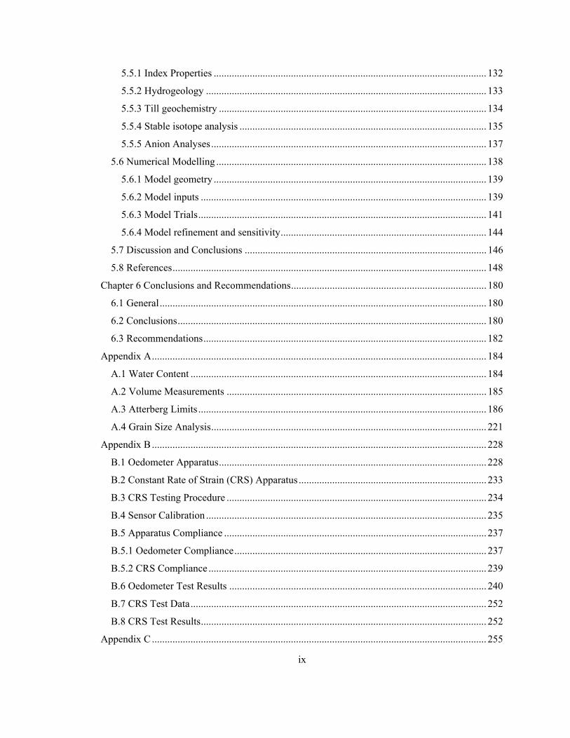
5.5.1 Index Properties .......................................................................................................... 132 5.5.2 Hydrogeology ............................................................................................................. 133 5.5.3 Till geochemistry ........................................................................................................ 134 5.5.4 Stable isotope analysis ................................................................................................ 135 5.5.5 Anion Analyses........................................................................................................... 137
5.6 Numerical Modelling ......................................................................................................... 138 5.6.1 Model geometry .......................................................................................................... 139 5.6.2 Model inputs ............................................................................................................... 139 5.6.3 Model Trials................................................................................................................ 141 5.6.4 Model refinement and sensitivity................................................................................ 144
5.7 Discussion and Conclusions .............................................................................................. 146 5.8 References.......................................................................................................................... 148
Chapter 6 Conclusions and Recommendations............................................................................ 180 6.1 General............................................................................................................................... 180 6.2 Conclusions........................................................................................................................ 180 6.3 Recommendations.............................................................................................................. 182
Appendix A.................................................................................................................................. 184 A.1 Water Content ................................................................................................................... 184 A.2 Volume Measurements ..................................................................................................... 185 A.3 Atterberg Limits................................................................................................................ 186 A.4 Grain Size Analysis........................................................................................................... 221
Appendix B .................................................................................................................................. 228 B.1 Oedometer Apparatus........................................................................................................ 228 B.2 Constant Rate of Strain (CRS) Apparatus ......................................................................... 233 B.3 CRS Testing Procedure ..................................................................................................... 234 B.4 Sensor Calibration ............................................................................................................. 235 B.5 Apparatus Compliance ...................................................................................................... 237 B.5.1 Oedometer Compliance.................................................................................................. 237 B.5.2 CRS Compliance ............................................................................................................ 239 B.6 Oedometer Test Results .................................................................................................... 240 B.7 CRS Test Data................................................................................................................... 252 B.8 CRS Test Results............................................................................................................... 252
Appendix C .................................................................................................................................. 255

x
C.1 Triaxial Swell Test - Sensor Calibration ........................................................................... 255 Appendix D.................................................................................................................................. 262
D.1 Model Development.......................................................................................................... 262 Appendix E .................................................................................................................................. 270
E.1 Core Sampling & Preservation .......................................................................................... 270

xi
List of Figures
Figure 2.1 Field site location in southern Saskatchewan............................................................ 33 Figure 2.2 Schematic of Denison core barrel (modified from Terzaghi et al., 1996)................. 34 Figure 2.3 Photograph of a typical core sample extruded from Denison core barrel. ................ 34 Figure 2.4 Typical oedometer time-deformation plot. ............................................................... 35 Figure 2.5 Typical oedometer results ......................................................................................... 35 Figure 2.6 (a) Casagrande method for determining preconsolidation pressure. (b) Butterfield
method for determining preconsolidation pressure................................................... 36 Figure 2.7 The influence of structure and quantifying sample disturbance in clay. (a) Effect of
structure on the compression behaviour of clay. (b) Lunne et al. (1997) criteria, (b)
Terzaghi et al (1996) criteria (c) Hong and Han (2007) criteria. .............................. 37 Figure 2.8 (a) Compressibility of oedometer apparatus. (b) Relationship between uncorrected
and corrected oedometer data. .................................................................................. 38 Figure 2.9 Photographs of core samples showing (a) shear plane in core 169 and (b) fracturing
and post sampling disturbance in core 181. .............................................................. 39 Figure 2.10 Oedometer specimen dimensions, diameter and target heights for the four different
sizes tested. ............................................................................................................... 39 Figure 2.11 Index properties fro the Bearpaw Shale. ................................................................... 40 Figure 2.12 Intrinsic compressibility from a variety of clays including the Bearpaw Formation.
(adapted from Burland, 1990 and Hinchberger, 2009). ............................................ 40 Figure 2.13 Oedometer results for four difference specimen sizes in relation the measured ICL
from the Bearpaw Formation (a) core 169 (41.75 – 43.25 mbgs), (b) core 185
(66.15-67.65 mbgs) and (c) core 202 (90.5-91.95 mbgs) ......................................... 42 Figure 2.14 Interpretation of preconsolidation pressure for different specimen sizes from core
185 (66.48-66.83m) (a) 63.5 mm diameter (b) 35.6 mm diameter (c) 25.0 mm
diameter and (d) 16.9 mm diameter. ......................................................................... 43 Figure 2.15 Quantifying disturbance for oedometer tests (a) Terzaghi et al. (1996) criterion (b)
Lunne et al. (1997) criterion. Shaded diamonds represent ‘good’ specimens, open
squares ‘poor’ specimens (25.0 and 16.9 mm diameter samples only)..................... 44 Figure 2.16 Preconsolidation pressure with depth (b) Change in void ratio with depth. Shaded
diamond represent ‘good’ specimens, open squares represent ‘poor’ specimens. .... 45

xii
Figure 2.17 Compression indexes from oedometer tests. Shaded symbols represent ‘good’
specimens, open symbols represent ‘poor’ specimens.............................................. 45 Figure 2.18 Consolidation parameters and the effect of specimen size (a) Coefficient of volume
compressibility, (b) Coefficient of consolidation and (c) Hydraulic conductivity.
Shaded symbols represent ‘good’ specimens, open symbols represent ‘poor’
specimens. ................................................................................................................. 47 Figure 3.1 (a) Field site location, southern Saskatchewan (b) Site geology and stratigraphy.... 68 Figure 3.2 Effect of secondary compression on the compression behaviour of a soil (a)
behaviour of a ‘young’ clay (b) behaviour of an ‘aged’ clay (c) influence of structure
on an ‘aged’ clay (modified after Bjerrum, 1967 and Tatsuoka, 2006). ................... 69 Figure 3.3 (a) Two loading increments from a multi-staged consolidation test (b) loading
increments from (a) expressed in terms of strain rate (c) isotache development for
multi-staged consolidation test and (d) incremental compression and swelling
indexes and relationship between preconsolidation pressure and strain rate. ........... 70 Figure 3.4 (a) CRS consolidation curves from two identical samples tested at different strain
rates and (b) relationship between preconsolidation pressure, strain rate and
secondary compression. ............................................................................................ 71 Figure 3.5 Disturbance criteria assessment for conducted oedometer and CRS tests. ............... 71 Figure 3.6 Isotache development for a 169 oedometer specimen. ............................................. 72 Figure 3.7 Isotache development for 202 oedometer specimen ................................................. 73 Figure 3.8 Comparison of MSL oedometer and CRS tests conducted (a) core 169 (41.75-
43.25m) and (b) core 202 (90.5-91.95m). ................................................................. 74 Figure 3.9 Comparison of all oedometer and CRS tests conducted ........................................... 75
Figure 3.10 Relationship between Cc* and Cαe and effective stress for all oedometer tests. ........ 76
Figure 3.11 Relationship between Cc*
and Cαe. ............................................................................ 76 Figure 3.12 Change in preconsolidation pressure with change in strain rate. .............................. 77 Figure 3.13 Typical oedometer unloading increment................................................................... 77
Figure 3.14 Cs* and Cαe versus effective stress for all oedometer tests. ....................................... 78
Figure 3.15 Relationship between Cc*
, Cs* and Cαe for all oedometer tests conducted. ................ 79
Figure 4.1 Infiltration boundary conditions and stress volume paths applied by laboratory
apparatus. ................................................................................................................ 102 Figure 4.2 Formation of clay minerals and structure of montmorillonite (after Craig, 1997).. 103 Figure 4.3 Swell pressure measurements (after Dixon et al. 2002).......................................... 104

xiii
Figure 4.4 Schematic of triaxial apparatus. .............................................................................. 105 Figure 4.5 Close up of pedestal base. ....................................................................................... 106 Figure 4.6 Photograph of specimen.......................................................................................... 106 Figure 4.7 Photograph of specimen in triaxial cell................................................................... 107 Figure 4.8 Effect of sample sizes on one-dimensional swell pressure measurements. ............ 108 Figure 4.9 Gravimetric water content versus swell pressure for one dimensional swell tests,
ultra small sized samples only. ............................................................................... 108 Figure 4.10 Void ratio versus swell pressure for one dimensional swell tests, ultra small sized
samples only............................................................................................................ 109 Figure 4.11 200 kPa Constant mean stress test results: mean stress, volume strain and water
added to sample versus time (core 169, 41.75 – 43.25 mbgs). ............................... 109 Figure 4.12 400 kPa Constant mean stress test results: mean stress, volume strain and water
added to sample versus time (core 169, 41.75 – 43.25 mbgs). ............................... 110 Figure 4.13 200 kPa Constant volume test results: mean stress, volume strain and water added to
sample versus time (core 169, 41.75 – 43.25 mbgs). .............................................. 110 Figure 4.14 400 kPa Constant volume test results: mean stress, volume strain and water added to
sample versus time (core 169, 41.75 – 43.25 mbgs). .............................................. 111 Figure 4.15 Mean stress versus time for infiltration tests........................................................... 111 Figure 4.16 Volume strain versus time for infiltration tests....................................................... 112 Figure 4.17 Water added to sample versus time for infiltration tests. ........................................ 112 Figure 4.18 Axial strain versus volume strain for both CMS and CV tests. .............................. 113 Figure 4.19 Radial strain versus volume strain for CMS and CV tests conducted. ................... 113 Figure 4.20 Axial versus radial strain for CMS and CV tests conducted................................... 114 Figure 4.21 Gravimetric water content versus mean stress. ....................................................... 114 Figure 4.22 Volume strain versus mean stress. .......................................................................... 115 Figure 4.23 Specific volume versus mean stress. ....................................................................... 115 Figure 4.24 End of test volume strain versus end of test mean stress. ....................................... 116 Figure 4.25 Swell pressure versus effective montmorillonite dry density(modified from Dixon,
2002). ...................................................................................................................... 116 Figure 4.26 Comparison between one dimensional swell pressure measurements, triaxial swell
tests. ........................................................................................................................ 117 Figure 4.27 Development of SELs. ............................................................................................ 117

xiv
Figure 5.1 Range of specific discharge over which diffusion or mechanical dispersion controls
hydrodynamic diffusion (modified from Rowe, 1987). .......................................... 155 Figure 5.2 Global meteoric water line (modified from Craig, 1961). ...................................... 156 Figure 5.3 Deviations from the meteoric water line resulting from potential fractionation
mechanisms (Clark and Fritz, 1997). ...................................................................... 156 Figure 5.4 Stratigraphy of southern Saskatchewan. ................................................................. 157 Figure 5.5 Location of field site in southern Saskatchewan..................................................... 158 Figure 5.6 Stratigraphic borehole log and location of samples used. Diamonds were sampled
from Nov 2005, Squares were sampled Sept 2006 and the circles are dried samples
used as part of this investigation from Remenda (1993). Shaded diamonds and
squares represent Shelby tube samples. .................................................................. 159 Figure 5.7 Geophysical logs from Sept 2006 drilling investigation. Resistivity and Spontaneous
Potential readings were unable to be obtained during cased section of the borehole as
indicated by the straight lines.................................................................................. 160 Figure 5.8 Squeezing apparatus used for pore water extraction consisting of Enerpac hand jack,
hydraulic cylinder and pressure gauge.................................................................... 161 Figure 5.9 Complete pore water extraction apparatus. ............................................................. 161 Figure 5.10 Close up view of pore water collection system....................................................... 162 Figure 5.11 Atterberg limits, density and porosity measurements conducted on both till and clay
samples.................................................................................................................... 162 Figure 5.12 Plasticity chart......................................................................................................... 163 Figure 5.13 Hydraulic conductivity versus void ratio, calculated from oedometer tests on the
Bearpaw Formation................................................................................................. 163 Figure 5.14 Till geochemistry – total carbonate and zinc within the till and the upper part of the
clay.......................................................................................................................... 164
Figure 5.15 Stable Isotope Geochemistry - δD and δ18O profiles with depth. ........................... 164 Figure 5.16 Stable isotopes results and the local meteoric water line for Saskatoon. Local
meteoric water line as given by Hendry and Wassenaar (1999). ............................ 165 Figure 5.17 Anion analysis (Cl- and SO4
-) for extracted pore water within the till and underlying
clay.......................................................................................................................... 165 Figure 5.18 SRC borehole log. ................................................................................................... 166 Figure 5.19 Model Scenario A, basal till deposition. ................................................................. 167

xv
Figure 5.20 Results for the King site, model scenario A. (a) results from ice cover stage of the
model only (b) final model results, including both ice cover and precipitation...... 168 Figure 5.21 Results for the Luck Lake site, model scenario A. (a) results from ice cover stage of
the model only (b) final model results, including both ice cover and precipitation.
................................................................................................................................. 169
Figure 5.22 Model scenario B, basal till deposition, initial δD values in the till -190. .............. 170 Figure 5.23 Results from model scenario B (a) king site (b) Luck Lake site............................. 171 Figure 5.24 Model scenario C, melt out till deposition, ice located directly on till during
glaciation................................................................................................................. 172 Figure 5.25 Result from model scenario C (a) King site (b) Luck Lake site. ............................ 173 Figure 5.26 Model scenario D, melt out till deposition at Luck Lake site, combination of ablation
and basal melt out till at the King site..................................................................... 174 Figure 5.27 Result from model scenario D (a) King site (b) Luck Lake site. ............................ 175 Figure 5.28 Model results for 20,000 years (10,000 ice cover + 10,000 precipitation) over a
variety of constant fluxes. ....................................................................................... 176 Figure 5.29 Model results for 25,000 years (15,000 ice cover + 10,000 precipitation) over a
variety of constant fluxes. ....................................................................................... 176 Figure 5.30 Model results for 30,000 years (20,000 ice cover + 10,000 precipitation) over a
variety of constant fluxes. ....................................................................................... 177 Figure 5.31 Model results with the effective diffusion coefficient equal to 3.5x10⁻¹⁰ m2/s in both
the till and clay for 20,000 years over a variety of fluxes. ...................................... 177 Figure 5.32 Model results using two effective diffusion coefficients: 3.5x10⁻¹⁰ m2/s in the till and
1.7x10⁻¹⁰ m2/s in the clay over 20,000 years. .......................................................... 178 Figure 5.33 Model results for a variety of time periods at a constant flux of 0.75 m per 10,000
years. ....................................................................................................................... 178 Figure 5.34 Model results for a variety of time periods at a constant flux of 1.0 m per 10,000
years. ....................................................................................................................... 179 Figure B.1 Photographs of oedometer apparatus ...................................................................... 229 Figure B.2 Specifications for 35.6 mm diameter cutter and collar assembly. .......................... 230 Figure B.3 Drawings for 25.0 mm diameter cutter and collar assembly................................... 231 Figure B.4 Drawings for 16.9 mm diameter cutter and collar assembly................................... 232 Figure B.5 Photographs of CRS apparatus. .............................................................................. 233 Figure B.6 Sensor Calibration (a) Load Cell (b) LVDT (c) Pressure transducer...................... 236

xvi
Figure B.7 Oedometer compliance test results.......................................................................... 237 Figure B.8 Example of adjustment to raw readings when corrected for compliance................ 238 Figure B.9 CRS compliance data. ............................................................................................. 239 Figure B.10 Load increments and determination of end of primary consolidation. (a) uncorrected
change in height, (b) corrected change in height accounting for oedometer
compressibility displaying end of primary consolidation, (c) fitted line for log-linear
portion before end of primary consolidation is complete, (d) fitted line for log-linear
portion after end of primary consolidation.............................................................. 244 Figure B.11 Unloading increments for a typical oedometer test: (a) uncorrected change in height,
(b) corrected change in height accounting for oedometer compressibility displaying
end of primary consolidation, (c) fitted line for log-linear portion before end of
primary consolidation is complete, (d) fitted line for log-linear portion after end of
primary consolidation. ............................................................................................ 248 Figure B.12 Summary plot for typical oedometer test. ............................................................... 249 Figure B.13 Example determination of Normally Consolidated Line and Unload-Reload line (Cc
and Cs)..................................................................................................................... 249 Figure B.14 Example determination of preconsolidation pressure. ............................................ 250 Figure B.15 Strain rate versus vertical strain for each loading increment. Red circles are
calculated data and black circles are interpolated data points................................. 251 Figure B.16 Calculated isotaches for a typical oedometer test. .................................................. 251 Figure B.17 Data outputs from data acquisition system for a typical CRS test. ......................... 253 Figure B.18 Summary plots for a typical CRS test. .................................................................... 253 Figure B.19 Preconsolidation pressure determination for CRS data........................................... 254 Figure D.1 (a) Luck Lake model geometry and (b) 1m spaced meshed model ........................ 266 Figure D.2 (a) SEEP/W model boundary conditions (b) Pressure head results showing water
table at 2m below ground surface. .......................................................................... 267 Figure D.3 CTRAN/W stages and boundary conditions (a) Initial material concentrations (b)
Stage 3 boundary conditions (initial) and (b) Stage 4 boundary conditions (initial).
................................................................................................................................. 268 Figure D.4 Time step determination for the model. .................................................................. 269 Figure E.1 Hydraulic piston core sample extruded................................................................... 271 Figure E.2 Sealed and waxed core samples. ............................................................................. 271

xvii
List of Tables
Table 2.1 Criteria for assessing disturbance and sample quality (after Lunne et al. 1997)....... 31 Table 2.2 Criteria for assessing disturbance and sample quality (after Terzaghi et al. 1996)... 31 Table 2.3 Testing matrix for first stage of oedometer testing ................................................... 31 Table 2.4 Testing matrix for second stage of oedometer testing............................................... 32 Table 2.5 Index Properties ........................................................................................................ 32 Table 2.6. Comparison of preconsolidation pressures for varying sample sizes and depths ..... 32 Table 4.1 Triaxial swell testing matrix. .................................................................................. 101 Table 4.2 Comparison of sample sizes used. ............................ Error! Bookmark not defined. Table 4.3 One dimensional swell pressure test results............................................................ 101 Table 4.4 Summary of end of test triaxial swell pressure tests. .............................................. 102 Table 5.1 Relative abundance for the stable isotopes of oxygen and hydrogen. .................... 152 Table 5.2 Water level readings................................................................................................ 152 Table 5.3 Till and Bedrock Geochemistry results................................................................... 153 Table 5.4 Carbonate contents from tills in southern Saskatchewan........................................ 153 Table 5.5 Zinc values from tills in southern Saskatchewan. ................................................... 154 Table 5.6 Model Boundary Conditions Luck Lake site. ......................................................... 154 Table 5.7 Model Boundary Conditions King site. .................................................................. 155 Table B.1 CRS Testing Matrix ................................................................................................ 252

xviii
List of Symbols and Abbreviations
αL longitudinal dispersivity
δ del (parts per thousand)
ε strain rate
εr radial strain
εa axial strain
εx strain in the x direction,
εv vertical strain
v Poisson’s Ratio, and
θ volumetric water content
ρ density
ρd dry density
ρw density of water
σv’ effective stress
σp’ preconsolidation pressure
σi’ effective stress of ith increment
σx,y,z total stress in the x, y or z direction
σr radial stress, and
τ tortuosity factor
1D one dimensional 2H or D deuterium 18O oxygen-18
A cross-sectional area
C concentration
Cαe secondary compression index
Cc compression index
Cc* compression index of load increment
Cs swelling index
Cs* swell index of load increment
cv coefficient of consolidation
De effective diffusion coefficient
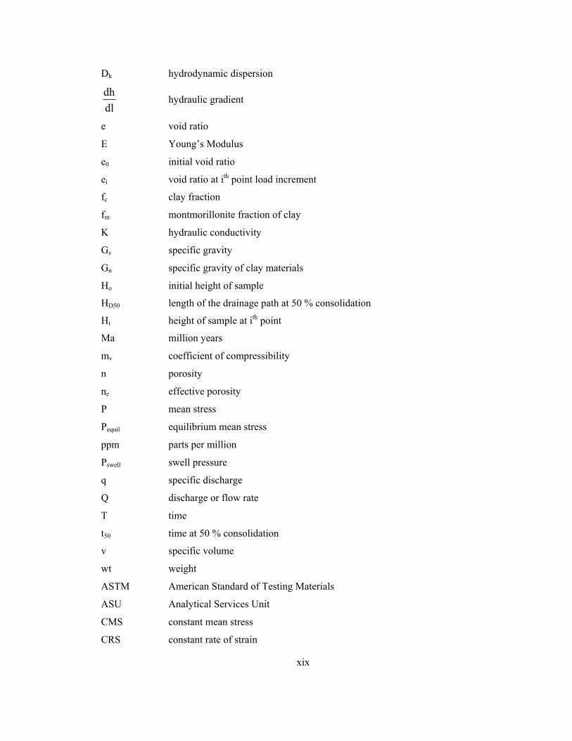
xix
Dh hydrodynamic dispersion
dldh
hydraulic gradient
e void ratio
E Young’s Modulus
e0 initial void ratio
ei void ratio at ith point load increment
fc clay fraction
fm montmorillonite fraction of clay
K hydraulic conductivity
Gs specific gravity
Gn specific gravity of clay materials
Ho initial height of sample
HD50 length of the drainage path at 50 % consolidation
Hi height of sample at ith point
Ma million years
mv coefficient of compressibility
n porosity
ne effective porosity
P mean stress
Pequil equilibrium mean stress
ppm parts per million
Pswell swell pressure
q specific discharge
Q discharge or flow rate
T time
t50 time at 50 % consolidation
v specific volume
wt weight
ASTM American Standard of Testing Materials
ASU Analytical Services Unit
CMS constant mean stress
CRS constant rate of strain

xx
CS constant stiffness
CV constant volume
DDW distilled deionized water
EMDD effective montmorillonite dry density
GMWL global meteoric water line
GWC gravimetric water content
ICL intrinsic compression line
LMWL local meteoric water line
LVDT linear variable displacement transformers
mbgs meters below ground surface
NCL normal compression line
VSMOW Vienna standard mean ocean water
RMS root mean squares
SCL sedimentation compression line
SEL swell equilibrium limit
USCS unified soil classification system
Chapter 1
Introduction
1.1 Background
Stiff clay shales exhibit behaviour that lies on the boundary between rock and soil, posing
many unique and interesting challenges when measuring and predicting their hydro-mechanical
behaviour. In many cases, standard soil testing equipment is not adequate for characterising such
a stiff material and conventional rock testing methods do not yield the constitutive parameters
required in many investigations. The difficulty associated with sampling and laboratory testing of
stiff soils results in a large percentage of past work being conducted on reconstituted specimens.
Although this allows tests to be performed, reconstituting soil removes all natural heterogeneities
and anisotropy within the material. While this form of testing provides useful information
regarding the remoulded material properties it cannot provide information regarding the influence
of structure, due to deposition and stress history, which can significantly affect the performance
and behaviour of the material.
In order to characterize the deformation characteristics of natural soils, the structure of
the in-situ material must be retained in the laboratory specimen. The effect of sample disturbance
is an issue continually faced by researchers working with soil samples. Quantifying and assessing
this disturbance is crucial to understanding and interpreting soil behaviour. There has been a
significant amount of research conducted on the effect of sample disturbance on soft soils. Many
researchers have found large differences in strength and stiffness parameters when comparing
specimens acquired from high versus low quality sampling techniques (Bjerrum, 1967; Lefebvre
and Poulin 1979; La Rochelle et al., 1981; Lacasse et al., 1985; Sandbaekken et al., 1986;
Leroueil and Kabbaj, 1987; Burland, 1990; Hight et al., 1992; Tan et al., 2002; Graham, 2006;
Lunne et al., 2006; Hong and Han, 2007). The combination of unloading stresses combined with

2
the difficulty in forming laboratory specimens in these stiff and brittle materials, makes it
challenging to work with when attempting to obtain representative specimens for a laboratory
test. It is hypothesised that small diameter specimens can be used to avoid discreet disturbed
zones (i.e. fractures) induced during sampling, as well as to enable application of high stress
conditions required to yield the material.
Time dependent behaviour of soils is important when evaluating the long term
performance of geotechnical structures. As design lives of geotechnical structures are continually
increasing the impact of creep behaviour becomes more important. For example, waste storage
applications can require engineers to guarantee structures for decades, and in the case of nuclear
waste storage thousands or even tens of thousands of years into the future. Soils undergo
secondary compression or creep defined as continued deformation under constant effective stress.
Given that creep processes occur in-situ and during laboratory testing, they must be accounted for
when interpreting material parameters and deriving geologic interpretations. For example,
preconsolidation pressure is a parameter commonly used to assess overburden stress history and
overburden thickness through time. In soft soils, it has been well established that an increase in
strain rate results in an increase in preconsolidation pressure (Leroueil et al, 1983; Leroueil et al,
1985; Leroueil, 1996). Currently, there is a lack of data in the literature on creep in stiff soils for
reasons outlined here. In order to properly design applications in stiff soils for use far into the
future and to properly interpret geologic history of these materials, creep behaviour needs to be
accounted for.
The ability for swelling soils to undergo large volume changes due to increase in
moisture content under constant stress, places many challenges on engineers as they try to
understand and mitigate the effects of working within these types of materials. Damage to
infrastructure due to swelling soils is measured in the billions of dollars every year (Keller, 2008).

3
On the positive side, waste storage applications exploit the swelling ability of these types of
materials in order to retain potential contaminants. Siemens and Blatz (2009) showed that swell
behaviour is heavily influenced by the applied boundary conditions. Their work led to the
development of a Swell Equilibrium Limit (SEL), defined as the limit to volume expansion and
confining stress that occurs during water infiltration under controlled boundary conditions. The
SEL provides a framework for the prediction of swell behaviour of the material and increases
understanding of swelling materials under wetting conditions. The SEL aims to increase the
accuracy of predicting the swelling behaviour of soils however, applicability of the SEL
framework in natural clay materials has not been satisfied to date as only engineered material
have been tested.
Stable isotopes in groundwater, particular deuterium (2H) and oxygen-18 (18O), are
commonly used as proxies of past hydrologic and climatic conditions resulting from the strong
correlation between temperature and isotopes in precipitation. Remenda et al. (1994) found that
thick unweathered clay deposits have the ability to maintain 18O signatures in pore waters for over
10,000 years, a direct result of the low permeability of such clay deposits. Additionally, stable
isotope distributions have been successfully used by others (Hendry and Wassenaar, 1999;
Remenda et al., 1996) to provide information on groundwater flow, solute transport mechanisms,
hydraulic conductivity, and the timing of climatic and geologic events. In many cases obtaining
an extensive vertical tracer profile with depth, in low permeability materials, to assess the timing
of geologic events as noted above is uncommon. Although the current database of tracer profiles
is limited, the ability for low permeable soils to retain fingerprints of past geologic events over
many years makes them ideal candidates for the study of long term behaviour or historical
analysis within the system when applicable.

4
1.2 Objectives
This thesis takes a multidisciplinary approach to comprehensively investigate the material
properties, mechanical properties and pore water chemistry of a stiff soil, to determine how these
properties relate to the strength of this material, and challenge our ideas of the hydrogeology and
the geological history of the region. Specific thesis objectives are to:
• Investigate in detail the material properties and characterize the compression behaviour
of Bearpaw shale. To accomplish this, the use of small-size specimens is also evaluated.
• Examine the time dependent behaviour of a stiff soil and the transferability of time rate
models developed in soft soils to stiff soils.
• Examine the swelling potential and behaviour of clay and determine the influence of
boundary conditions to this behaviour. Assess the applicability of the swell concepts
developed for compacted materials to a naturally swelling clay material.
• Constrain the depositional age of materials overlying the Bearpaw shale through the use
of stable isotope profiles and finite element modelling.
1.3 Methods
A field site, located roughly 160 km south of Saskatoon, near the towns of Birsay and
Lucky Lake, was selected for the following investigation. The site consists of 32 m of glacial till,
believed to be made up of both the Floral and Battleford Formations, overlying approximately 90
m of Cretaceous clay shale of the Bearpaw Formation.
The geology in this region is comprised of thick successions of clayey glacial tills,
deposited over six glaciations that overlie Cretaceous marine deposits. The glacial deposits have
been divided into two groups; the younger Saskatoon Group, and the underlying Sutherland
Group. The Saskatoon Group is subdivided into the Battleford and Floral Formations and the

5
Sutherland Group is subdivided into the Warman, Dundurn and Mennon Formations. The
Bearpaw Formation which underlies the glacial deposits is the youngest formation of the
Montana Group (71-72 Ma). It is comprised of alternating marine silty clays and sands that were
deposited during the Campanian to early Maastrichtian. The Snakebite Member, one of eleven
members of the Bearpaw Formation (Caldwell, 1968), forms the bedrock surface over much of
southern Saskatchewan and is comprised of non-calcareous marine silt and clay. The Snakebite
Member overlies the Ardkenneth Member, a non-calcareous marine, very fine – to fine grained
sand and silt aquifer that sources domestic and agricultural uses within the area.
Drilling and the collection of core samples, in both the till and clay, was conducted on
two separate occasions using both Shelby tubes and Denison core barrels. Water level data and
water samples were also collected using existing piezometers installed on site. In addition to the
investigations above, dried samples collected during earlier investigations on site (Remenda,
1993) were used to provide complimentary laboratory analysis for this research.
A series of laboratory tests were conducted both at Queen’s University and the Royal
Military College to examine the material properties, the compression characteristics, the time
dependent behaviour, the swell potential and the pore water chemistry of the sampled material.
1.4 Organization of Thesis
This thesis is presented in an extended manuscript format. Due to the multidisciplinary
nature of this work and the wide range of topics covered, the addition of relevant background
information was incorporated into each section to facilitate understanding across the different
subject areas. Where required, this background information will be omitted prior to submission of
the manuscripts. In Chapter 2 the material properties and compression behaviour of the Bearpaw
is investigated, in addition to assessing specimen size and disturbance within this material. In
Chapter 3 strain rate effects and the transferability of time dependent models developed for soft

6
soils to a stiff clay are investigated. In Chapter 4 the natural swell behaviour of the Bearpaw were
examined through a series of one dimensional and specialized triaxial swell tests conducted under
controlled boundary conditions. In Chapter 5 re-examination of the till stratigraphy, at the study
location, was conducted through the investigation of till geochemistry, pore water chemistry from
both the till and underlying Cretaceous deposits and finite element modelling. A summary and
discussion of the work undertaken as well as recommendations for future work is presented in
Chapter 6.

7
1.5 References
Bjerrum, L. 1967. Progressive failure of slopes of overconsolidated plastic clay and clay shales. Proceedings of the American Society of Civil Engineers, Journal of the Soil Mechanics and Foundations Divisions, 93, 2–49. Burland, J.B. 1990. On the compressibility and shear strength of natural clays. Géotechnique, 40(3), 329–378. Caldwell, W.G.E. 1968. The Late Cretaceous Bearpaw Formation in the South Saskatchewan River valley. Saskatchewan Research Council, Geology Division, Report #5 Graham, J. 2006. The 2003 R.M. Hardy Lecture: Soil parameters for numerical analysis in clay. Canadian Geotechnical Journal. 43, 187-209. Hendry, M.J. and Wassenaar, L.I. 1999. Implications of the distribution of δD in pore waters for groundwater flow and the timing of geologic events in a thick aquitard system. Water Resources Research, 35, 1751-17560. Hight, D. W., Bond, A. J., & Legge, J. D. (1992). Characterization of the Bothkennar clay: an overview. Géotechnique, 42 (2), 303-347 Hong, Z., and Han, J. 2007. Evaluation of Sample Quality of Sensitive Clay Using Intrinsic Compression Concept. Journal of Geotechnical and Geoenvironmental Engineering. ASCE. 83-90. Keller, EA. 2008. Environmental geology, Eighth Edition. Prentice Hall. USA LaRochelle, P., Sarrailh, J., Tavenas, F., Roy, M., and Leroueil, S. 1981. Causes of sampling disturbance and design of a new sampler for sensitive soils. Canadian Geotechnical Journal, 18(1), 52–66. Lacasse, S., Berre, T., and Lefebvre, G. 1985. Block sampling of sensitive clays. Proceedings 11th ICSMFE, San Francisco, 2, 887-892. Lefebve, G. and Poulin, C. 1979. A new method of sampling in sensitive clay. Canadian Geotechnical Journal. 16. 226-233. Leroueil, S. 1996. Compressibility of Clays: Fundamental and Practical Aspects. Journal of Geotechnical Engineering, ASCE, 122(7), 534-543. Leroueil, S., Tavenas, F., Samson, L and Morin, P. 1983. Preconsolidation pressure of Champlain clays. Part II. Laboratory determination. Canadian Geotechnical Journal, 20 803-816. Leroueil, S., Kabbaj, M., Tavenas, F and Bouchard, R. 1985. Stress-strain-strain rate relation for the compressibility of sensitive natural clays. Géotechnique, 35(2), 159-180.

8
Leroueil, S. and Kabbaj, M. 1987. Discussion of ‘Settlements analysis of embankments on soft clays’ by G. Mesri and Y.K. Choi. Journal of Geotechnical Engineering, ASCE. 113(9), 1067-1070. Lunne, T., Berre, T., Andersen, K.H., Strandvik, S., Sjursen, M. 2006. Effects of sample disturbance and consolidation procedures on measured shear strength of soft Norwegian clays. Canadian Geotechnical Journal, 43, 726-750. Remenda, V.H. 1993. Origin and migration of natural groundwater tracers in thick clay tills of Saskatchewan and the Lake Agassiz clay plain. PhD Thesis. University of Waterloo. Remenda, V.H., Cherry, J.A., and Edwards, T.W.D. 1994. Isotopic composition of old ground water from Lake Agassiz: implications for late Pleistocene climate. Science 266, 1975-1978 Remenda, V.H., G. van der Kamp, and J.A. Cherry. 1996. Use of vertical profiles in delta18O to constrain estimates of hydraulic conductivity in a thick, unfractured till. Water Resources Research, 32 (10), 2979–2987. Siemens, G.A. and Blatz, J.A. 2009. Evaluation of the influence of boundary confinement on the behaviour of unsaturated swelling clay soils. Canadian Geotechnical Journal, 46(3), 339–356 Sandbaekken, G., Berre, T., and Lacasse, S. 1986. Oedometer testing at the Norwegian Geotechnical Institute. In Consolidation of soils: testing and evaluation. Edited by R.N. Yong and F.C. Townsend. American Society for Testing and Materials (ASTM), Special Technical Publication STP 892, 329–353 Tan, T.S., Lee, F.H., Chong, P.T., and Tanaka, H. 2002. Effect of sampling disturbance on properties of Singapore clay. Journal of Geotechnical and Geoenvironmental Engineering, ASCE, 128, 898–906.

9
Chapter 2
Characterization of the Bearpaw Shale in oedometric compression.
2.1 Introduction
There has been a significant amount of research conducted into the effect of sample
disturbance on soft soils (Graham, 2006; Hight et al., 1992; Lacasse et al., 1985; Lefebvre and
Poulin 1979; Leroueil, S. and Kabbaj, M., 1987), from which the general rule adopted is that the
larger the sample the more representative of in situ behaviour. In contrast, there has been little
work done on very stiff, hard soils. These soils typically exhibit behaviour that lies on the
boundary between rock and soil, posing many unique and interesting challenges when conducting
laboratory tests. In many cases, standard soil test equipment is not adequate for testing such a stiff
material and, conventional rock testing methods do not yield the constitutive parameters required
in many investigations. For example, ASTM D 4546 (ASTM, 1996) requires that the
preconsolidation pressure be exceeded by four times in the conventional oedometer frame. In stiff
soils with preconsolidation pressures anticipated to be 6000-10000 kPa, achieving four times the
preconsolidation pressure using traditional sized specimens is not possible.
Stiff, hard soils are often located at depth making it difficult and costly to obtain
undisturbed samples. The extensive unloading that is experienced by the soil upon sampling
results in large suctions to develop, and the formation of fractures which are uncharacteristic of
the material in its natural state. Bjerrum (1967) found that unloading of stiff clay resulted in
disintegration and fracturing. In addition, the stiff brittle nature of these materials makes it
difficult to work with when trying to acquire representative samples for a laboratory test. If the
entire core is used to characterize the compressibility of the material, the likelihood of obtaining a
partially disturbed specimen is substantially increased. This poses the question of whether a small
oedometer, to test smaller specimens extracted from less disturbed regions from the core, would

10
mitigate this problem and produce more reliable results. It is hypothesized that the testing of
smaller diameter specimens may therefore give more representative bulk material properties than
larger specimens.
Sample disturbance can also be introduced into the specimen during preparation. The
minimum recommended aspect ratio (diameter-to-height ratio) for an oedometer specimen is 2.5
however a ratio of greater than 4 is preferable in order to minimize the effects of sidewall friction
(ASTM, 1996). In very stiff clays, the brittle nature of these materials makes it extremely difficult
to obtain a thin, large diameter specimen without damaging it. It is further hypothesized that a
reduced aspect ratio of the specimens in stiff clays could reduce disturbance to the specimen.
A field site, located roughly 160 km south of Saskatoon near the towns of Birsay and
Lucky Lake, was selected for the following investigation as shown in Figure 2.1. The site consists
of 30 m of glacial till overlying approximately 90 m of the Snakebite Member of the Bearpaw
Formation. The Bearpaw Formation, youngest formation of the Montana Group (71-72 Ma), is a
westward thinning wedge of predominately marine silty clays and sands, overlying the Judith
River and Lea Park Formations. The Snakebite Member forms the bedrock surface over much of
southern Saskatchewan and is comprised of non-calcareous marine silt and clay deposited at a
slow rate in relatively quiet waters (Caldwell, 1968). Subsequent deposition and glaciation have
resulted in an overconsolidated clay which is now in a state of rebound following erosion and
unloading (Peterson, 1958). Clay shale of the Bearpaw Formation was extensively studied during
the construction of the Gardiner Dam in southern Saskatchewan. Peterson (1954) found that the
shale could be divided into, an upper, middle and lower zone. The upper zone was soft with high
water content ranging from 29-36 % that contained many slickensides and joint planes. The lower
zone consisted of uniform, hard shale that had limited number of slickensides and joints with
water contents ranging from 20-27 %. The middle zone defined the transition between the upper

11
to lower zones, contained numerous fractures and exhibited water contents ranging from 25-31
%.
Sauer and Misfeldt (1993) examined the preconsolidation pressures in a variety of
Cretaceous clays from southern Saskatchewan and found that values range from 11,000 to 12,000
kPa in the Bearpaw. They noted that the preconsolidation pressures observed in the clays were
significantly higher than estimates from stratigraphy evidence however the effects of secondary
compression contribution were minimal.
In stiff clays the most common accepted method for sampling is with a Denison core
barrel, comprised of an outer rotating barrel and an inner fixed barrel with a liner that is used to
collect the sample, shown in Figure 2.2. Drilling was conducted in September 2006 with
Saskatchewan Department of Highways using a hydraulic rotary drill. Washed cuttings were
taken during the entire length of the borehole, which was cased to the till/clay contact to facilitate
sampling over multiple days. Three 0.6 m long Shelby tubes were collected near the till/clay
contact until the clay became sufficiently stiff that the Shelby tubes would no longer penetrate the
clay. Following this, nine 1.5 m Denison core barrels were collected every 5 m between 42 and
92 m within the Bearpaw Formation. Evidence of bentonite lenses, shell fragments and large
concentration (a hard, compact aggregate of mineral matter) layers were observed during the
investigation. A photograph of a typical core sample extracted from a Denison core barrel is
presented in Figure 2.3. Further details on core sampling and preservation are given in Appendix
E.
The material properties and compression behaviour of the Bearpaw Shale are investigated
in this chapter. In addition, the difficulty in obtaining good quality samples, resulting from the
stiff, brittle nature of the material, led to the assessment of specimen size and disturbance prior to
the investigation.

12
2.2 Background
2.2.1 Consolidation Testing
The behaviour of material during one-dimensional swelling and consolidation is
determined using a standard oedometer test in which the specimen is compressed under pressure
and the deformation measured (ASTM, 1996). The specimen is confined laterally and allowed to
drain vertically in both directions. A vertical load is applied to the specimen causing excess pore
pressure to develop. The excess pore pressures induce a hydraulic gradient and water flows out of
the specimen causing settlement or consolidation to occur. The vertical deformation of the
specimen is measured, typically over a 24 hour period at which time the excess pore pressures
have completely dissipated and the applied pressure is equal to the effective stress in the
specimen. The parameters to be determined from a consolidation test include the coefficient of
compressibility, coefficient of consolidation, coefficient of secondary compression, hydraulic
conductivity and preconsolidation pressure. Their definitions are presented in this section.
2.2.1.1 Coefficient of Compressibility
The coefficient of volume compressibility, mv, is defined as the volume change per unit
increase in effective stress for a unit volume of soil (Craig, 1997). The volume change may be
expressed in terms of void ratio or specimen thickness as seen in Equation 2.1.
⎟⎟⎠
⎞⎜⎜⎝
⎛−
−=⎟⎟
⎠
⎞⎜⎜⎝
⎛−
−+
=+
+
+
+''
1
1
0''
1
1
0
11
1
ii
ii
ii
iiv
HHH
eee
mσσσσ
2.1
where:
e0 = initial void ratio
ei = void ratio at beginning of load increment
ei+1 = void ratio at end of load increment
σi’ = effective stress of previous load increment

13
σi+1’ = effective stress of current load increment
Ho = initial height of sample
Hi = height of sample at beginning of load increment
Hi+1 = height of sample at end of load increment
2.2.1.2 Coefficient of Consolidation
The coefficient of consolidation, cv, is calculated for each load increment using the
deformation-time plot. There are two methods used to determine cv however only the log-time
method will be discussed here. Figure 2.4 shows a typical time-deformation plot. End of primary
consolidation is determined by the intersection of a tangent line to the normal compression line
and a tangent line to the secondary compression curve. To determine the start of initial
compression two point on the curve (a, b) that have a time ratio of 4:1 are selected. The vertical
distance between these points is then set off above the first point which corresponds to d0. Once
d50 and d100 have been determined d50 and t50 can be solve for. The coefficient of consolidation
can then be calculated using Equation 2.2.
50
2D
v tH197.0
c 50= 2.2
where:
cv = coefficient of consolidation
HD50 = length of the drainage path at 50 % consolidation
t50 = time at 50 % consolidation
2.2.1.3 Compression Indexes
Figure 2.5 shows the typical behaviour of a soil undergoing one dimensional
consolidation. The compression index, Cc, shown in Figure 2.5, is the slope of the normal
compression line as given by Equation 2.3.

14
( )'0
'1
10c log
eeC
σ−σ−
= 2.3
where:
e0 = initial void ratio over increment examined
e1 = end void ratio over increment examined
σ0’ = effective stress at e0
σ1’ = initial effective at e1
The swelling index, Cs, is the slope of the rebound or swell line shown in Figure 2.5 and is given
by Equation 2.4.
( )'0
'1
10s log
eeC
σ−σ−
= 2.4
where:
e0 = initial void ratio over increment examined
e1 = end void ratio over increment examined
σ0’ = effective stress at e0
σ1’ = initial effective at e1
2.2.1.4 Preconsolidation Pressure
The preconsolidation pressure (σp’) is a yield point that describes the onset of significant
plastic deformations during compressive loading. There are a number of different methods that
have been developed to determine the preconsolidation pressure, two of the most common are
discussed below. Casagrande (1936) developed a graphical method for the determination of σp’,
shown in Figure 2.6(a). The point of maximum curvature is located, point A, at which a
horizontal and tangent lines are drawn. The bisector to the horizontal and tangents lines is then
drawn. The straight line of line normal compression line is extended back to the bisector. The
intersection of these two lines is the preconsolidation pressure. Butterfield (1979) developed a

15
method in which the consolidation data is plotted in ln(1+e) versus ln (σv) instead of the
traditional e versus log σv plot. In this method σp’ is defined as the point of intersection of two
straight lines that extend from the linear section of each end of the compression curve as seen in
Figure 2.6(b).
2.2.2 Soil Compressibility
2.2.2.1 Structure and Intrinsic Compression Line (ICL)
An important characteristic of stiff clays is the presence of structure. Structure is
commonly divided into macrostructure and microstructure. Macrostructure is defined as fractures,
joints, stratification and other visible features, whereas microstructure is developed from a
combination of fabric and bonding (Mitchell, 1993). There are a number of geological processes
that allow for the development of natural structure in clay such as mechanical unloading leading
to overconsolidation and changes in the physical or chemical composition of the material through
cementation or diagenesis.
The intrinsic properties of soils are considered to be the basic or inherent properties of the
material, independent of the natural state or absent of structure. Burland (1990) defined intrinsic
properties as properties from a reconstituted specimen that have been mixed at water contents
ranging from 1 to 1.5 times the liquid limit. By reconstituting the material at high water contents
the soil loses its memory related to soil structure and thus its stress history. When tested in a
laboratory the compression behaviour of the reconstituted specimen produces the intrinsic
compression line (ICL) as shown in Figure 2.7a. The ICL enables the independent comparison of
material behaviour to undisturbed core samples which depend not only on mineralogy of the clay
and its pore water chemistry but the deposition and consolidation conditions or structure with the
soil.

16
The influence of structure has been shown by others (Burland, 1990; Leroueil and
Vaughan, 1990; Gasparre et al, 2007) to increase the pre-yield stiffness of the material and lead to
higher yield stress and strength as illustrated in Figure 2.7a. Leroueil and Vaughan (1990) found
that microstructure was equally important as void ratio and stress history, in determining the
behaviour of a material and thus a necessary consideration when interpreting laboratory analysis.
Figure 2.9a illustrates the typical compression behaviour between a disturbed and undisturbed
structured sample when tested in the laboratory. As the sample becomes increasingly disturbed
the pre-yield stiffness decreases and compression curves moves in the direction of the ICL.
2.2.2.2 Disturbance and Specimen Quality
Sample disturbance results from the destruction of natural structure present in a material.
The presence of structure influences the material behaviour and thus deviations from this natural
state are not reflective of the material’s in-situ behaviour. The effect of disturbance in
consolidation testing has been well documented in soft soils (Sandbaekken et al., 1986; Leroueil
and Kabbaj, 1987; Hight et al, 1992; Grozic et al., 2003; Graham, 2006). The typical effects of
disturbance are an increase in compressibility during recompression and a decrease in
preconsolidation pressure. This disturbance becomes increasingly important when examining the
stiffness of a material which is greatly affected by disturbance or lack of structure. To mitigate
this disturbance in soft soils, alternative sampling methods have been developed (Lefebvre and
Poulin 1979; Lunne et al., 2006) to increase the quality and subsequent size of the sample. In the
case of stiff soils, often located a great depth, sampling quickly becomes costly and challenging
due to the increased strength of the material.
Quantifying the amount of disturbance is important to assess the sample quality of the
specimens tested as it can mask the natural behaviour of the clay. Lunne et al. (1997) developed a
criterion for sample disturbance in which the change of void ratio during reconsolidation to the
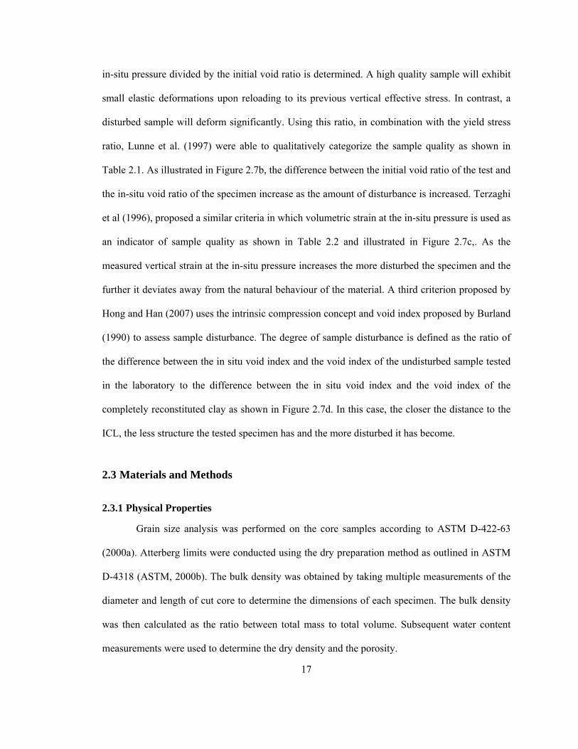
17
in-situ pressure divided by the initial void ratio is determined. A high quality sample will exhibit
small elastic deformations upon reloading to its previous vertical effective stress. In contrast, a
disturbed sample will deform significantly. Using this ratio, in combination with the yield stress
ratio, Lunne et al. (1997) were able to qualitatively categorize the sample quality as shown in
Table 2.1. As illustrated in Figure 2.7b, the difference between the initial void ratio of the test and
the in-situ void ratio of the specimen increase as the amount of disturbance is increased. Terzaghi
et al (1996), proposed a similar criteria in which volumetric strain at the in-situ pressure is used as
an indicator of sample quality as shown in Table 2.2 and illustrated in Figure 2.7c,. As the
measured vertical strain at the in-situ pressure increases the more disturbed the specimen and the
further it deviates away from the natural behaviour of the material. A third criterion proposed by
Hong and Han (2007) uses the intrinsic compression concept and void index proposed by Burland
(1990) to assess sample disturbance. The degree of sample disturbance is defined as the ratio of
the difference between the in situ void index and the void index of the undisturbed sample tested
in the laboratory to the difference between the in situ void index and the void index of the
completely reconstituted clay as shown in Figure 2.7d. In this case, the closer the distance to the
ICL, the less structure the tested specimen has and the more disturbed it has become.
2.3 Materials and Methods
2.3.1 Physical Properties
Grain size analysis was performed on the core samples according to ASTM D-422-63
(2000a). Atterberg limits were conducted using the dry preparation method as outlined in ASTM
D-4318 (ASTM, 2000b). The bulk density was obtained by taking multiple measurements of the
diameter and length of cut core to determine the dimensions of each specimen. The bulk density
was then calculated as the ratio between total mass to total volume. Subsequent water content
measurements were used to determine the dry density and the porosity.

18
2.3.2 Sample Disturbance
Two examples of the disturbance seen within the samples are shown in Figure 2.9,
disturbance due to in-situ shearing and stress release and post sampling disturbance. Oedometer
specimens ranging in size from 63.5 mm to 16.9 mm in diameter, as shown in Figure 2.10, were
examined in order to assess whether a smaller sized specimen reduces disturbance, producing
representative compression behaviour of a stiff clay. The minimum ASTM standard aspect ratio
is 2.5 however a ratio of greater than 4 is recommended to minimize the effects of sidewall
friction (ASTM, 1996). An aspect ratio of 4.8 was used in the 63.5 mm diameter oedometer. For
the smaller diameter specimens (36.5 mm, 25.0 mm and 16. 9 mm) an aspect ratio of 2.5 was
used. This coincides with the maximum aspect ratio used when testing cylindrical rock specimens
(ASTM, 2008)
2.3.3 Consolidation Testing
Consolidation testing was divided into two types, reconstituted and undisturbed. The
reconstituted consolidation tests were performed to acquire the intrinsic compression line of the
material. A dried sample of core was selected, crushed and then mixed to a water content of
200% before being placed in a 63.5 mm diameter oedometer. The sample was loaded to a
pressure of 1800 kPa upon which it was unloaded to 100 kPa. From this consolidated specimen a
smaller 25.0 mm diameter specimen was extracted and then consolidation to a maximum load of
32 MPa.
The multi-staged oedometer tests were conducted in two stages. The first stage was to
assess the validity of using smaller specimen sizes. The second stage was to further quantify
disturbance and quality of samples. During the first sage of testing, 12 one dimensional
oedometer tests were conducted on three different depth core samples, one from the top, one from
the middle and one from the bottom of the sampled region. Testing of these samples was

19
completed using four different diameter samples ranging in size from 63.5 mm to 16.9 mm as
outlined in Table 2.3. To accommodate the testing of smaller diameter specimens, development
of new sample cutters and collars were undertaken to utilize the existing base assemblies for each
of the oedometers. The 63.5 mm diameter cutters came with the oedometer apparatus and
represent the standard testing size used. A set of 35.6 mm sized cutter rings were also pre-
existing, however the top collar assembly and a suitable top cap that fit the existing oedometer
base and loading arm were required. Additionally a 25.0 mm and a 16.9 mm sized samples were
completely non-standard and thus development of cutting rings, collars and top caps were
required. Detailed specification and drawings of the cutting rings, collar and tops caps for all
35.6, 25.0 and 16.9 mm diameter samples can be found in Appendix B. Slight modification to the
oedometer hanger rod took place, where the rod was lengthened to accommodate more weight (a
maximum of 200 kg) during the tests. The second stage of testing consisted of 8 additional
oedometer tests, six with 16.9 mm diameter specimens and two with a 25.0 mm diameter as
shown in Table 2.4.
The one dimensional consolidation tests were conducted in a standard oedometer
apparatus with water uptake conducted under constant volume conditions as given by Method C
in ASTM D 4546 and analyzed using the log-time method (ASTM 1996). Displacement
measurements were taken with a Wykeham Ferrance 0.002 mm accuracy dial gauge. To reduce
the amount of evaporation during the length of the test, plastic was used to cover the water bath.
Loading increments occurred every 24 hours unless end of primary consolidation was not
achieved during that time period at which point subsequent time was allowed to pass in order for
equilibrium of pore pressures to be achieved.

20
2.3.4 Apparatus Compliance
The compressibility of the oedometer apparatus was measured and accounted for in the
testing program. A steel sample of similar diameter and height to the actual soil specimens tested
was placed in the oedometer cells and loaded incrementally until the maximum load of 200 kg
was applied, followed by unloading. The results from a typical compliance test and its duplicate
are shown in Figure 2.8 (a). Similar methods for determining apparatus compliance have been
used and found to be successful by other researchers (Kalidindi et al., 1997; Cotecchia, 1996).
For each oedometer test the same set of porous stones corresponding to the soil tests were used in
the compliance testing. Hysteresis is observed between the initial loading and unloading, however
to ensure consistency and repeatability, each compliance test was duplicated. This was done by
completely disassembling the apparatus then reassembling and performing additional compliance
tests.
2.4 Test results
2.4.1 Index Properties
Index properties, including Atterberg limits, density and porosity of the clay are given in
Table 2.5 and depicted in Figure 2.11. Liquid and plastic limits range from 99 to 145% and 22 to
29%, respectively with an average water content of 23%. Average grain size was found to be 7%
sand, 54% silt and 39% clay with local variation in the individual cores. Plasticity of the clay
ranges from 74 to 122% and thus is denoted as high plasticity by the Unified Soil Classification
System (USCS) (ASTM, 2000c).
2.4.2 Compliance Correction
Prior to the analysis of the data, the oedometer readings were corrected for machine
compressibility. As discussed previously, each oedometer test had its own compliance correction

21
to reflect the conditions under which the test was conducted. Figure 2.8(b) compares using only
the loading curve and then using both the unloading and loading curves to correct the data. The
difference between the correction using both the unloading and loading curves in comparison to
just using the loading was negligible under the stress interval tested, as the slopes of the normal
compression line (Cc) and the rebound line (Cs) were unchanged between the two curves.
Therefore, only the loading curve was used to correct the data. To apply the correction, a function
was assigned to the appropriate loading curve which was then used to adjust the oedometer
readings to account for the apparatus compressibility that would be present over that particular
stress interval. From Figure 2.8(b) it can be seen that the corrected curve is shifted upward as the
apparatus compressibility is removed from the readings. This shift is less in the low stress portion
of the curve however becomes more significant in the higher stress portion of the curve. The
corrected curve results in a larger preconsolidation pressure as well as lower values for the
normal compression line (Cc) and the rebound line (Cs) and therefore failing to correct for
apparatus compressibility would underestimate these parameters.
2.4.3 Oedometer Testing
2.4.3.1 Intrinsic Compression Line (ICL)
The intrinsic compression line was determined, from a reconstituted sample taken from
the 169 core (41.75 – 43.25 mbgs), in accordance with the method outlined by Burland (1990).
The ICL for the Bearpaw shale is presented in Figure 2.12 and found to be consistent to that of
other highly plastic clays. It has been documented by others (Burland, 1990 and Hinchberger and
Qu, 2009) that the ICL is influenced by the liquid limit of the material. From Figure 2.11 it can be
seen that the liquid limits of the sampled cores are within a similar range until a depth of 80 mbgs
at which they decrease slightly. Although the ICL was performed on a sample of the 169 core, it

22
is deemed acceptable for all cores to a depth of 80 m but also provides a good baseline for
comparison with the deeper cores, although it may not entirely be applicable to those specimens.
2.4.3.2 Effect of sample size
The oedometer results presented in Figure 2.13 show the variation in compression
behaviour with the size of specimen tested from cores at three different depths. It can be seen that
in all cases the 63.5 mm and 35.6 mm diameter specimens appear to be more disturbed than the
two smaller specimens. The 25.0 mm and 16.9 mm specimens produce consistent results in all
cases and show a well developed normal compression line. This is supported by the position of
the consolidation curve to the measured ICL that the more disturbed samples plot closer or below
the ICL. This disturbance is attributed to a variety of factors the most important being the
laboratory preparation of the oedometer specimens. The large unloading experienced by the
sample promotes fracturing and suction developing in the sample which is magnified by the
manner in which an oedometer specimen prepared. Due to the extreme stiffness and low water
contents, the sampled material behaves in a brittle and blocky manner. When attempting to obtain
a large oedometer sample, the process of pushing a cutter into the core sample promotes the
propagation of existing fractures, causing substantial internal disturbance to the acquired
specimen. The larger the size of the specimen, the larger the area over which the sample is able to
separate and fracture within the confines of the cutter ring. In contrast, a small oedometer
specimen minimizes the area of being disturbed. In addition, the reduced size enables more
control when extracting a specimen from the core and minimizes the amount of internal fractures
that may be present with the specimen thereby producing a more representative sample.
Preconsolidation pressures were determined using the Butterfield (1979) method however
manual calculations using the Casagrande (1936) method were used to verify the results.
Modifications to the Butterfield method by plotting log (1 + e) against log p’ have been

23
successfully used in the past to determine preconsolidation pressures (Grozic et al., 2003;
Sridharan et al., 1991). Table 2.6 contains the preconsolidation pressure measurements for each
of the specimen sizes at three depths. It can be seen that the 63.5 mm and 36.5 mm diameter
specimens yield much lower preconsolidation pressures in comparison to the other two diameters
tests which are very similar to one another. An example of this is shown in Figure 2.14 where it
can clearly be seen that the 63.5 mm and in some cases the 36.5 mm diameter samples do not
exactly reach the normal compression line (NCL). Determining the preconsolidation pressure for
the 63.5 mm and 35.6 mm diameter specimens is speculative and questionable due to the chosen
NCL which is based on two points and is not consistent with the other sized specimens. This
highlights the importance of understanding the material in which you are testing and to be
cautious about the number of points measured after the preconsolidation pressure. If only the 63.5
mm and 35.6 mm sizes were tested, the resultant preconsolidation pressures would be incorrect
and misleading. It is not until higher stresses and subsequently less disturbed samples are
achieved, through the use of smaller specimen sizes, that the depiction of the NCL is seen.
In addition to the effect of size and disturbance on the preconsolidation pressure
measurements, the determined values are sensitive to the inherent variation resulting from the
subjectivity in which the preconsolidation pressures are determined. Both the Casagrande and
Butterfield methods require straight line determination, however due to the high yield stress of
this material, a slight shift in these fitted lines can greatly affect the determined preconsolidation
pressure. In the case of lightly overconsolidated soils, a shift in the fitted lines generally results in
a change of preconsolidation pressure on the order of one or ten kilopascals, whereas in this case
a slight shift in the curve results in a change on the order of hundreds or thousands kilopascals
and thus much more significant.

24
2.4.4 Assessing Disturbance
As seen previously, the 25.0 mm and 16.9 mm size oedometer specimens produce the
most accurate compression results. To further assess sample quality, additional oedometer tests
conducted at the selected sizes were examined in detail. To date, all the criteria developed to
assess sample disturbance have been for soft soils and as seen with specimen size this knowledge
may not directly transferrable. During testing it was noted that core 195 had been rotated within
the inner core barrel during sampling and would behave as a remoulded, disturbed specimen. This
disturbed specimen provided a baseline for the following disturbance analysis to assess how
applicable the soft soil criteria are to stiff soils. Figure 2.15(a) depicts the results of the Terzaghi
et al. (1996) criteria. Based on yield stress measurements conducted in this study as well as
previous measurements (Sauer and Misfeldt, 1993) the yield stress ratio for these sample should
be greater than 8 due to the large preconsolidation pressures in relation to the current in-situ
stress. It can be seen that four specimens plot with ratios of less than this and therefore
determined to be disturbed even though one of the specimens appears to plot in the A column.
The two remoulded 195 specimens plot in the D and B columns as illustrated in Figure 2.15(a).
The results from the Lunne et al. (1997) criterion are shown in Figure 2.15(b). This criterion has
only been quantified for stress ratios less than 4, however in the Bearpaw stress ratios are much
larger. It can be seen that the same four specimens deemed as disturbed using the Terzaghi et al
(1996) criteria plot as disturbed with this criterion. A cut off of 0.02 is proposed as a distinction
between the good quality and that of lesser quality specimens for stiff material using the Lunne et
al (1997) method. The method proposed by Hong and Han (2007) was inapplicable as it requires
the in-situ stress be above the ICL which is not the case for this material as seen in Figure 2.13.

25
2.4.5 Discussion
In order to accurately characterize the material and compression characteristics of the
Bearpaw shale the effect of sample size and an assessment of specimen disturbance was
conducted. It was seen that smaller diameter specimens allow for increased stress during the tests,
which in turn allow for a clearer depiction of the normal compression line. In addition, smaller
diameter specimens produce more reliable, less disturbed results.
Preconsolidation pressure measurements for the 25.0 mm and 16.9 mm oedometer sizes,
alongside the change in void ratio with depth are shown in Figure 2.16. It was seen earlier (Figure
2.14) that with the two larger diameter specimens the NCL was not achieved as the maximum
load applied was insufficient to each normal consolidation. Therefore, the preconsolidation
pressures were not obtained. If however, the maximum load could have been increased to
sufficiently depict the NCL, it was seen that these larger diameter specimens were more disturbed
and would have yielded lower preconsolidation pressures than the smaller diameter specimens.
This is consistent with what is seen by other researchers (Leroueil, 1996 and Graham, 2006) in
soft soils. Preconsolidation determination in the 63.5 mm and 35.6 mm diameter specimens is
suspect and inconsistent and was therefore removed from the detailed analysis. The overall trend,
as shown by the dashed line in Figure 2.16, shows the preconsolidation pressure at a minimum
value of 4.5 MPa near the till/shale interface increasing to a maximum value of 10 MPa at a depth
of 67 m below which the values remain constant. The reduced preconsolidation pressure near the
surface of the till/clay interface is attributed to softening. This is supported by the increased water
content values seen in the upper 30 m of the shale from Figure 2.11. Additionally, the presence of
slickensides and shear planes were noted in core samples at depths above 67 m as shown in
Error! Reference source not found..
The resultant compression indices from the conducted oedometer tests are shown in
Figure 2.17. Typically in soft soils the difference between the compression and swelling index is

26
on the order of 10, whereas in this case the values are only differing by a factor of 4. Although it
appears that the 63.5 mm diameter oedometers yield comparable Cc values to the smaller
diameters and only the 35.6 mm oedometer produce poor values, it was clearly seen in Figure
2.14 that the 63.5 and 35.6 mm specimens did not reached the NCL and therefore the measured
Cc are not correct.
Time dependent consolidation parameters such as volume compressibility, coefficient of
consolidation and hydraulic conductivity are presented in Figure 2.18 (a), (b) and (c). It can be
seen that mv and cv yield similar trends with largest value (more compressible) at low effectives
stresses, decreasing in an exponential manner with increased stress. However, it is seen in Figure
2.18 (a) that the disturbed samples result in higher mv values compared with the undisturbed
samples at low effective stresses. As the effective stress increases the differences between the
disturbed and undisturbed become negligible suggesting the effect of sample disturbance is
minimal at high effective stress only. The overall trend of the disturbed and undisturbed samples
in Figure 2.18 (b) is comparable indicating the effect of sample disturbance is minimal on the
determination of cv. The relationship between calculated hydraulic conductivity and void ratio is
linear with increasing void ratio yielding increased hydraulic conductivity as expected as seen in
Figure 2.18 (c). As with mv and cv, K does not appear to be influenced by size and thus
disturbance.
2.5 Conclusions
In stiff soils, the extensive unloading that a sample exhibits during sample collection
promotes fracturing within the sample. This fracturing is magnified when trying to obtain
laboratory specimens representative of the in-situ behaviour of the material. Applying the
experience gained with soft soils would suggest using large sampling tube sizes are required to
obtain representative results. However in stiff soils, the brittle nature and lower water content

27
prove to be problematic when trying to obtain large oedometer specimens. It has been shown that
reduced specimen sizes, when working with a stiff soil, minimizes the effect of disturbance and
produces more accurate results. The decreased specimen size also aids in the determination
preconsolidation pressure by not only reducing the disturbance to the sample, resulting from
unloading, but enables these high stresses to be achieved in conventional testing equipment.
Assessing disturbance in a stiff soil is not straightforward but a necessary step resulting
from the structure present in these types of material. Two criterions developed by Terzaghi et al.
(1996) and Lunne et al. (1997) were used to assess disturbance with the oedometer specimens.
Overall, the methods provide a good baseline of assessing disturbance however there is much less
gradation to the quality of a specimen in stiff soil. It was found that the specimen was deemed
either good quality or poor quality with no variability in between.
Detailed characterization of the Bearpaw clay shale was conducted. The depth of
softening was identified through the measured preconsolidation profile with low values (4.5 MPa)
at the till/clay interface, gradually increasing to a depth of 67 m and a maximum value of 10 MPa
below which the values were constant. Parameters Cc and σp’ were highly sensitive to sample
disturbance however other parameters such as cv and k were less dramatically affected by
disturbance. Therefore, care must be taken when assessing the compression of a stiff soil as
failing to achieve sufficiently higher stresses and the presence of disturbed specimens may lead to
misleading Cc and σp’ values.

28
2.6 References
American Society for Testing and Materials (ASTM). 1996. Standard Test Methods for One-Dimensional Swell or Settlement Potential of Cohesive Soils. Annual Book of Standards, Section 4, Soil and Rock (1). Vol 04-08. D 4546-96. ASTM International, West Conshohocken, Pennsylvania. American Society for Testing and Materials (ASTM). 2000a. Standard Test Method for Particle-Size Analysis of Soils. Annual Book of Standards, Section 4, Soil and Rock (1). Vol 04-08. D 422-63. ASTM International, West Conshohocken, Pennsylvania. American Society for Testing and Materials (ASTM). 2000b. Standard Test Methods for Liquid Limit, Plastic Limit and Plasticity Index of Soils. Annual Book of Standards, Section 4, Soil and Rock (1). Vol 04-08. D 4318-00. ASTM International, West Conshohocken, Pennsylvania. American Society for Testing and Materials (ASTM). 2000c. Standard Practice for Classification of Soils for Engineering Purposes (Unified Soil Classification System). Annual Book of Standards, Section 4, Soil and Rock (1). Vol 04-08. D 2487-00. ASTM International, West Conshohocken, Pennsylvania. American Society for Testing and Materials (ASTM). 2008. Standard Practices for Preparing Rock Core as Cylindrical Test Specimens and Verifying Conformance to Dimensional and Shape Tolerances. Annual Book of Standards, Section 4, Soil and Rock (1). Vol 04-08. D 4543-08. ASTM International, West Conshohocken, Pennsylvania. Bjerrum, L. 1967. Progressive failure of slopes of overconsolidated plastic clay and clay shales. Proceedings of the American Society of Civil Engineers, Journal of the Soil Mechanics and Foundations Divisions, 93, 2–49. Burland, J.B. 1990. On the compressibility and shear strength of natural clays. Géotechnique, 40(3), 329–378. Butterfield, R. 1979. A natural compression law for soils. Géotechnique,29: 469–480. Caldwell, W.G.E. 1968. The Late Cretaceous Bearpaw Formation in the South Saskatchewan River valley. Saskatchewan Research Council, Geology Division, Report #5 Casagrande, A. 1936. The determination of the pre-consolidation load and its practical significance. In Proceedings of the 1st International Soil Mechanics and Foundation Engineering Conference, Cambridge, Mass., 22–26 June 1936. Edited by A. Casagrande. Graduate School of Engineering, Harvard University, Cambridge, Mass. Vol. 3, pp. 60–64 Cotecchia, F. 1996. The effect of structure on the properties of an Italian Pleistocene clay. PhD Thesis. University of London. Imperial College of Science, Technology and Medicine Craig, R.F. 1997. Soil Mechanics, Sixth Edition. E & FN SPON, London.

29
Gasparre, A., Nishimura, S., Coop, M. R. & Jardine, R. J. (2007). The influence of structure on the behaviour of London Clay. Géotechnique 57(1), 19-31 Graham, J. 2006. The 2003 R.M. Hardy Lecture: Soil parameters for numerical analysis in clay. Canadian Geotechnical Journal. 43. 187-209. Grozic, J.L.H., Lunne, T., and Pande, S. 2003. An oedometer test study on the preconsolidation stress of glaciomarine clay. Canadian Geotechnical Journal. 40, 857-872. Hinchberger, S.D and Qu, G. 2009. Viscoplastic constitutive approach for rate sensitive structured clays. Canadian Geotechnical Journal, 49 609-626. Hight D.W., Bond A.J. & Legge J.D. 1992. Characterisation of the Bothkennar clay: an overview. Géotechnique 42 303-348. Hong, Z., and Han, J. 2007. Evaluation of Sample Quality of Sensitive Clay Using Intrinsic Compression Concept. Journal of Geotechnical and Geoenvironmental Engineering. ASCE. 83-90. Kalidindi, S.R., Abuseafieh, A. and El-Danaf, E. 1997. Accurate Characterization of Machine Compliance for Simple Experimental Mechanics. 27(2), 210-215 Lacasse, S., Berre, T., and Lefebvre, G. 1985. Block sampling of sensitive clays. Proceedings 11th ICSMFE, San Francisco, 2, 887-892. Lefebve, G. and Poulin, C. 1979. A new method of sampling in sensitive clay. Canadian Geotechnical Journal. 16. 226-233. Leroueil, S. and Kabbaj, M. 1987. Discussion of ‘Settlements analysis of embankments on soft clays’ by G. Mesri and Y.K. Choi. Journal of Geotechnical Engineering, ASCE. 113(9), 1067-1070. Leroueil, S., and Vaughan, P.R. 1990. The general and congruent effects of structure in natural soils and weak rocks. Géotechnique, 40(3), 467–488. Lunne, T., Berre, T., Andersen, K.H., Strandvik, S., Sjursen, M. 2006. Effects of sample disturbance and consolidation procedures on measured shear strength of soft Norwegian clays. Canadian Geotechnical Journal, 43, 726-750. Lunne, T., Berre, T. & Strandvik, S. 1997. Sample disturbance effects in soft low plastic Norwegian clay. Proceedings of the international symposium on recent developments in soil and pavement mechanics, Rio de Janeiro, pp. 81–102. Mitchell, J.K. 1993. Fundamentals of Soil Behaviour, Wiley, New York, USA. Peterson, R. 1954. Studies of Bearpaw shale at a dam site in Saskatchewan, Proc. ASCE, New York, v.80, separate no. 476.

30
Peterson, R. 1958. Rebound in the Bearpaw Shale, Western Canada. GSA Bulletin, 69, 1113-1124. Sandbaekken, G., Berre, T., and Lacasse, S. 1986. Oedometer testing at the Norwegian Geotechnical Institute. In Consolidation of soils: testing and evaluation. Edited by R.N. Yong and F.C. Townsend. American Society for Testing and Materials (ASTM), Special Technical Publication STP 892, 329–353 Sauer, E.K. and Misfeldt, G.A. 1993. Preconsolidation of Cretaceous Clays of the Western Interior Basin in Southern Saskatchewan. Proceeding of the 46th Annual Canadian Geotechnical Conference, Saskatoon, Saskatchewan. September 27-29. Sridharan, A., Abraham, B.M., and Jose, B.T. 1991. Improved technique for estimation of preconsolidation pressure. Géotechnique, 41(2), 263-268. Terzaghi, K., Peck, R.B., and Mesri, G. 1996. Soil Mechanics in Engineering Practice. Third Edition. Wiley-Interscience.

31
Table 2.1 Criteria for assessing disturbance and sample quality (after Lunne et al. 1997)
δe/eo Yield stress
ratio Very good to
excellent Good to fair Poor Very Poor
1-2 <0.04 0.04-0.07 0.07-0.14 >0.14 2-4 <0.03 0.03-0.05 0.05-0.10 >0.10
Table 2.2 Criteria for assessing disturbance and sample quality (after Terzaghi et al. 1996).
Volumetric strain (%)
Specimen quality designation (SQD)
<1 A 1-2 B 2-4 C 4-8 D >8 E
Table 2.3 Testing matrix for first stage of oedometer testing
Specimen ID Diameter (mm) Depth (mbgs) 169L 63.5 42.50 169M 35.6 42.50 169S 25.0 42.50
169US 16.9 42.50 185L 63.5 66.90 185M 35.6 66.90 185S 25.0 66.90
185US 16.9 66.90 202L 63.5 90.86 202M 35.6 90.86 202S 25.0 90.86
202US 16.9 90.86

32
Table 2.4 Testing matrix for second stage of oedometer testing.
Specimen ID
Diameter (mm)
Depth (mbgs)
177US 16.9 54.70 177S 25.0 54.70
181US 16.9 60.85 189US 16.9 73.65 195US 16.9 80.00
195USB 16.9 80.00 198US 16.9 85.18 198S 25.0 85.18
Table 2.5 Index Properties
Sample ID
Depth (m)
Water Content
(%)
Plastic Limit (%)
Liquid Limit (%)
Plasticity Index (%)
Density (Mg/m3)
Dry Density (Mg/m3)
Porosity
169 42.50 29 23 145 122 1.95 1.49 0.45 177 54.70 26 23 135 113 1.98 1.54 0.43 181 60.85 23 22 128 106 2.04 1.64 0.40 185 66.90 23 27 138 111 2.06 1.66 0.39 189 73.65 22 29 137 108 2.08 1.72 0.38 195 80.00 21 24 111 87 2.04 1.67 0.39 198 85.18 19 25 99 74 2.09 1.73 0.36 202 90.86 21 25 109 84 2.05 1.67 0.38
Table 2.6. Comparison of preconsolidation pressures for varying sample sizes and depths
Specimen ID: 169 185 202
Dia. (mm) σp’ (kPa)
σp’ (kPa)
σp’ (kPa)
63.5 1438 2717 3042 36.5 3987 5663 6192 25.0 4550 9120 9026 16.9 4623 9890 10791

33
Figure 2.1 Field site location in southern Saskatchewan.

34
Figure 2.2 Schematic of Denison core barrel (modified from Terzaghi et al., 1996).
Figure 2.3 Photograph of a typical core sample extruded from Denison core barrel.
76 mm
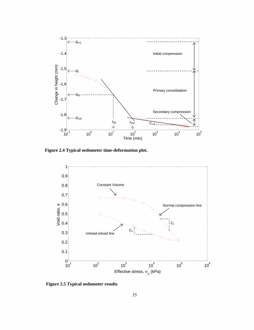
35
10-1
100
101
102
103
104
105-1.9
-1.8
-1.7
-1.6
-1.5
-1.4
-1.3
Time (min)
Cha
nge
in h
eigh
t (m
m)
Figure 2.4 Typical oedometer time-deformation plot.
101
102
103
104
105
1060
0.1
0.2
0.3
0.4
0.5
0.6
0.7
0.8
0.9
1
Effective stress, σv' (kPa)
Void
ratio
, e
Figure 2.5 Typical oedometer results
t100
d0
d50
d100 t50
dt=0
Primary consolidation
Secondary compression
Initial compression
Cαe
Normal compression line
Unload-reload line
Cc
Cs
Constant Volume

36
101
102
103
104
105
1060
0.1
0.2
0.3
0.4
0.5
0.6
0.7
0.8
0.9
1
Effective stress, σv' (kPa)
Voi
d ra
tio, e
(a)
2 3 4 5 6 7 8 9 10 11 120.1
0.15
0.2
0.25
0.3
0.35
0.4
0.45
0.5
0.55
0.6
Ln (σv' ) (kPa)
Ln(1
+e)
(b)
Figure 2.6 (a) Casagrande method for determining preconsolidation pressure. (b)
Butterfield method for determining preconsolidation pressure.
A
σp’ = 9472 kPa
σp’ = 9890 kPa

37
Figure 2.7 The influence of structure and quantifying sample disturbance in clay. (a) Effect
of structure on the compression behaviour of clay. (b) Lunne et al. (1997) criteria, (b)
Terzaghi et al (1996) criteria (c) Hong and Han (2007) criteria.

38
Vertical effective stress, σv' (kPa)
102 103 104 105 106
Def
orm
atio
n of
por
ous
ston
e (m
m)
-0.5
-0.4
-0.3
-0.2
-0.1
0.0
Apparatus CompressibiltyDuplicate
(a)
Vertical effective stress, σv' (kPa)
101 102 103 104 105 106
Sam
ple
heig
ht (m
m)
4.5
5.0
5.5
6.0
6.5
7.0
7.5
UncorrectedCorrected loading curveCorrected loading & unloading curve
(b)
Figure 2.8 (a) Compressibility of oedometer apparatus. (b) Relationship between
uncorrected and corrected oedometer data.

39
(a) (b)
Figure 2.9 Photographs of core samples showing (a) shear plane in core 169 and (b)
fracturing and post sampling disturbance in core 181.
Figure 2.10 Oedometer specimen dimensions, diameter and target heights for the four
different sizes tested.
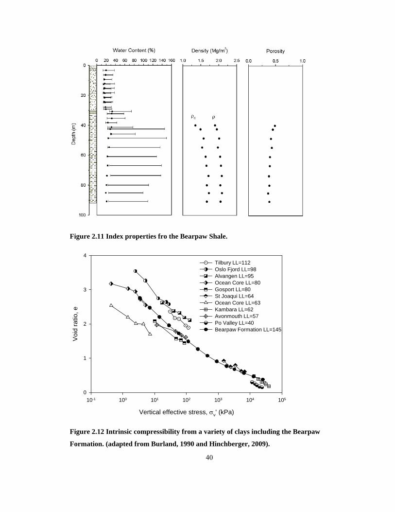
40
Figure 2.11 Index properties fro the Bearpaw Shale.
Vertical effective stress, σv' (kPa)
10-1 100 101 102 103 104 105
Voi
d ra
tio, e
0
1
2
3
4Tilbury LL=112Oslo Fjord LL=98Alvangen LL=95Ocean Core LL=80Gosport LL=80St Joaqui LL=64Ocean Core LL=63Kambara LL=62Avonmouth LL=57Po Valley LL=40Bearpaw Formation LL=145
Figure 2.12 Intrinsic compressibility from a variety of clays including the Bearpaw
Formation. (adapted from Burland, 1990 and Hinchberger, 2009).
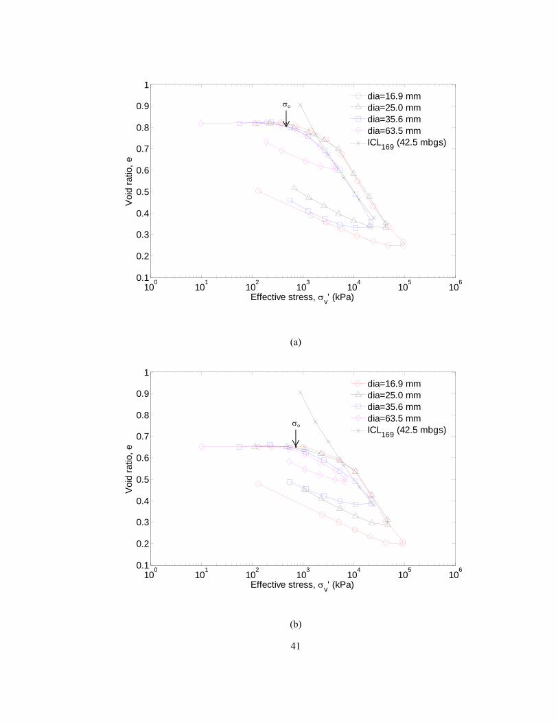
41
100
101
102
103
104
105
1060.1
0.2
0.3
0.4
0.5
0.6
0.7
0.8
0.9
1
Effective stress, σv' (kPa)
Voi
d ra
tio, e
dia=16.9 mmdia=25.0 mmdia=35.6 mmdia=63.5 mmICL169 (42.5 mbgs)
(a)
100
101
102
103
104
105
1060.1
0.2
0.3
0.4
0.5
0.6
0.7
0.8
0.9
1
Effective stress, σv' (kPa)
Voi
d ra
tio, e
dia=16.9 mmdia=25.0 mmdia=35.6 mmdia=63.5 mmICL169 (42.5 mbgs)
(b)
σo
σo

42
100
101
102
103
104
105
1060.1
0.2
0.3
0.4
0.5
0.6
0.7
0.8
0.9
1
Effective stress, σv' (kPa)
Voi
d ra
tio, e
dia=16.9 mmdia=25.0 mmdia=35.6 mmdia=63.5 mmICL169 (42.5 mbgs)
(c)
Figure 2.13 Oedometer results for four difference specimen sizes in relation the measured
ICL from the Bearpaw Formation (a) core 169 (41.75 – 43.25 mbgs), (b) core 185 (66.15-
67.65 mbgs) and (c) core 202 (90.5-91.95 mbgs)
σo
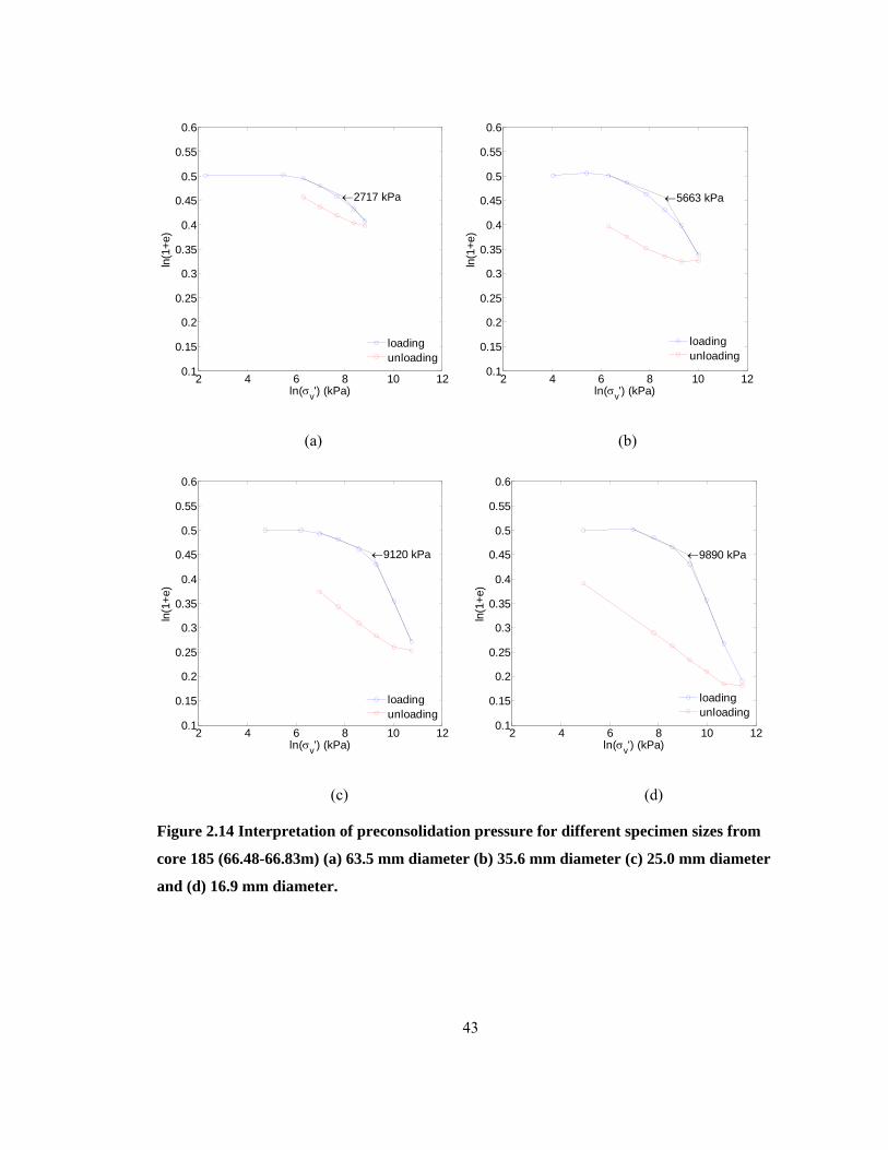
43
2 4 6 8 10 120.1
0.15
0.2
0.25
0.3
0.35
0.4
0.45
0.5
0.55
0.6
←2717 kPa
ln(σv') (kPa)
ln(1
+e)
loadingunloading
2 4 6 8 10 120.1
0.15
0.2
0.25
0.3
0.35
0.4
0.45
0.5
0.55
0.6
←5663 kPa
ln(σv') (kPa)
ln(1
+e)
loadingunloading
(a) (b)
2 4 6 8 10 120.1
0.15
0.2
0.25
0.3
0.35
0.4
0.45
0.5
0.55
0.6
←9120 kPa
ln(σv') (kPa)
ln(1
+e)
loadingunloading
2 4 6 8 10 120.1
0.15
0.2
0.25
0.3
0.35
0.4
0.45
0.5
0.55
0.6
←9890 kPa
ln(σv') (kPa)
ln(1
+e)
loadingunloading
(c) (d)
Figure 2.14 Interpretation of preconsolidation pressure for different specimen sizes from
core 185 (66.48-66.83m) (a) 63.5 mm diameter (b) 35.6 mm diameter (c) 25.0 mm diameter
and (d) 16.9 mm diameter.

44
-4 -2 00
2
4
6
8
10
12
14
16
Vertical strain, εv (%)
Stre
ss ra
tio
0 0.05 0.10
2
4
6
8
10
12
14
16
de/eo
Stre
ss ra
tio
(a) (b)
Figure 2.15 Quantifying disturbance for oedometer tests (a) Terzaghi et al. (1996) criterion
(b) Lunne et al. (1997) criterion. Shaded diamonds represent ‘good’ specimens, open
squares ‘poor’ specimens (25.0 and 16.9 mm diameter samples only).
E-VG G-F P
P E-VG VP G-F
B D A C
δe/do

45
0 5000 100000
10
20
30
40
50
60
70
80
90
100
Preconsolidation pressure, σp'(kPa)
Dep
th b
elow
gro
und
surfa
ce (m
)
-0.1 0 0.10
10
20
30
40
50
60
70
80
90
100
de/eo
Dep
th b
elow
gro
und
surfa
ce (m
)
(a) (b)
Figure 2.16 Preconsolidation pressure with depth (b) Change in void ratio with depth.
Shaded diamond represent ‘good’ specimens, open squares represent ‘poor’ specimens.
0 0.2 0.4 0.640
50
60
70
80
90
100
Dep
th b
elow
gro
und
surfa
ce (m
)
Cc
0 0.1 0.2 0.3 0.4
Cs
dia=16.9 mm dia=25.0 mm dia=35.6 mm dia=63.5 mm
Figure 2.17 Compression indexes from oedometer tests. Shaded symbols represent ‘good’
specimens, open symbols represent ‘poor’ specimens.
Till
Shale
σo
δe/do

46
102
103
104
105
1060
1
2
3
4
5
6
7
8 x 10⁻⁵
Effective stress, σv' (kPa)
mv (m
2 /kN
) ←y=0.0019x-0.6102
dia=16.9 mmdia=25.0 mmdia=35.6 mmdia=63.5 mm
(a)
102
103
104
105
1060
0.5
1
1.5
2
2.5
3
3.5
4
4.5 x 10⁻⁸
Effective stress, σv' (kPa)
c v (m2 /s
)
←y=9E-7x-0.5415
dia=16.9 mmdia=25.0 mmdia=35.6 mmdia=63.5 mm
(b)

47
10-14
10-13
10-12
10-11
10-100.1
0.2
0.3
0.4
0.5
0.6
0.7
0.8
0.9
1
1.1
Hydraulic conductivity, K (m/s)
Voi
d ra
tio, e
y=0.0918Ln(x)+3.1368→
dia=16.9 mmdia=25.0 mmdia=35.6 mmdia=63.5 mm
(c)
Figure 2.18 Consolidation parameters and the effect of specimen size (a) Coefficient of
volume compressibility, (b) Coefficient of consolidation and (c) Hydraulic conductivity.
Shaded symbols represent ‘good’ specimens, open symbols represent ‘poor’ specimens.

48
Chapter 3
Time dependent behaviour of the Bearpaw Shale in oedometric loading
and unloading
3.1 Introduction
Time or strain rate dependent behaviour of a soil is important when evaluating the long
term performance of many geotechnical structures such as tunnels, embankments and
excavations. Since the work of Suklje (1957) and Bjerrum (1967) on delayed deformation theory,
a significant amount of work has gone into developing models to describe the compressibility of
soft soils. From these studies, a number of different models have been developed to describe this
behaviour (Suklje, 1957; Leroueil et al., 1985; Yin and Graham, 1999; Mesri and Godlewski,
1977). While the literature on the compressibility of soft soils is extensive, work conducted on the
compressibility of stiff soils is limited (Hendron et al, 1969). In fact some have found that creep
is insignificant in stiff clays. Sauer and Misfeldt (1993) examined creep, in Cretaceous clays from
southern Saskatchewan, and found it was not measurable or significant.
Strain rate effects can have a significant influence on the compressibility characteristics
of natural materials. Under constant stress conditions in-situ soils continue to undergo secondary
compression or creep throughout geological history. This has the potential to mask the historical
stress parameters of the material if not taken into account properly. For example, the
preconsolidation pressure measured in a material that exhibits creep will not equal the maximum
overburden stress leading to a potential overestimation of overburden thickness. Sauer and
Misfeldt (1993) found that deformations due to creep were not measureable, however, the
preconsolidation pressures seen in the material were too large to be attributed to overburden stress
and a discrepancy arose that could not be attributed to another external factor. The limited data in
the literature on creep in stiff soil is a result of a combination of factors. The difficulty and cost of

49
sampling makes acquiring these samples prohibitive in many cases. In addition, the high
preconsolidation pressures associated with these types of materials do not allow proper definition
of deformation parameters in standard oedometer equipment.
In this chapter, it is hypothesized that rate dependent theories, developed primarily for
soft clays, are equally applicable to stiff highly overconsolidated clay shales. A field site, located
roughly 160 km south of Saskatoon near the towns of Birsay and Lucky Lake, was selected to
obtain samples of clay shale with preconsolidation pressures on the order of 10 MPa. The
stratigraphy of the site consists of 30 m of glacial till overlying approximately 90 m of the
Snakebite Member of the Bearpaw Formation (Figure 3.1). Recent investigations (Chapter 5)
revealed that the glacial till is part of the Battleford Formation, deposited during the retreat of the
last glaciation approximately 22,500 and 27,500 years ago. The Bearpaw Formation, the youngest
formation of the Montana Group (71-72 Ma), is a westward thinning wedge of predominately
marine silty clays and sands, overlying the Judith River and Lea Park Formations. The Snakebite
Member, one of eleven members of the Bearpaw Formation (Caldwell, 1968), forms the bedrock
surface over much of southern Saskatchewan and is comprised of non-calcareous marine silt and
clay deposited at a slow rate in relatively quiet waters. Subsequent deposition and glaciation have
resulted in overconsolidated clay which is now in believed to be in a state of rebound following
erosion and unloading (Peterson, 1958). Work conducted previously (Chapter 2), revealed that
the use of small specimens best characterizes the behaviour of a stiff material. The objective of
this paper is to characterize the time-dependent behaviour of Bearpaw Shale through the use of
oedometer and constant rate of strain testing on high quality specimens.

50
3.2 Background
3.2.1 Geological History
The Bearpaw Formation was deposited in the Campanian to early Maastrichtian during
the last major transgression and regression of the Cretaceous Bearpaw Sea. Volcanic activity in
south-western Montana occurred at various times during the deposition of the Bearpaw Formation
resulting in layers of volcanic ash within the sedimentary sequence (Scott & Brooker, 1968).
Deposition continued through the early Tertiary until the sediments reach a maximum elevation,
hypothesized at being upwards of 1000m as only sections of them remain today (Dawson et al.,
1994). Subsequent tectonic uplift and isostatic rebound began a period of significant erosion and
minor deposition throughout the remainder of the Tertiary. In southern Saskatchewan, Pliocene
sediments of the Empress group, comprised of lower preglacial and an upper proglacial unit, are
one of the few Tertiary deposits still present today. Glaciation within the region began around 1.8
million years ago (Fenton et al, 1994) depositing thick successions, from at least six glaciations,
of glacial tills throughout the region. Schrenier (1990) showed that the Quaternary stratigraphy is
a mirror image of the Cretaceous bedrock sequence resulting from the progressive stripping of the
underlying bedrock during glaciation. During this glacial stripping, rock was removed from the
Precambrian Shield and lower Cretaceous sandstones south of the shield then deposited as glacial
till over southern Saskatchewan.
The above sequence of events has led to a series of deposition and erosional periods
following the initial deposition of the Bearpaw Formation. Estimates of the preconsolidation
pressures in a variety of Cretaceous clays from southern Saskatchewan were studied by Sauer and
Misfeldt (1993) in which the values within the Bearpaw Formation range from 11,000 to 12,000
kPa. Through the examination of glacial tills in the region, Sauer et al. (1993) found the applied

51
stress from glacial loading to be 1800 ± 200 kPa suggesting the influence of glaciation on the
Bearpaw Formation is negligible.
3.2.2 Preconsolidation Pressure & Secondary Compression
The preconsolidation pressure is a yield point that describes the onset of significant
plastic deformations during compressive loading. For a normally consolidated recently deposited
soil (Figure 3.2a) the yield point corresponds to its maximum overburden stress. This is shown
diagrammatically in Figure 3.2a. Here we have an in-situ soil that is following a sedimentation
compression line to a void ratio of eo at an overburden stress of σvo. When tested in the
laboratory, such a sample will have a preconsolidation pressure equal to the maximum
overburden stress. However, if the same soil is held at constant stress in-situ it will decrease in
void ratio at constant stress illustrated in Figure 3.2b. If this second sample is then tested in the
laboratory it will yield a preconsolidation pressure of σ’p1, which is in excess of the maximum
overburden stress. The magnitude of this effect is a function of the number of log cycles of time
prior to sampling. This is illustrated in Figure 3.2b by the contours of constant time which are
parallel to the NCL and describe the change in void ratio at constant stress. Another complexity is
propensity for soils under sustained loading to develop microstructure. If such a process were to
occur the preconsolidation pressure can exceed that of Figure 3.2b as shown in Figure 3.2c. As a
result of all these competing processes the geological history of ancient sediments is very difficult
to assess from a single value such as preconsolidation pressure.
Secondary compression or creep is the deformation of a soil under constant effective
stress. Creep deformations are due to the gradual readjustment of clay particles into a more stable
arrangement, following disturbance of the skeletal structure by compression (Craig 1997). Ladd
et al. (1977) proposed two theories used to describe the stress-strain behaviour of soft soils

52
following primary consolidation. The secondary compression index, Cαe, is defined as the change
in void ratio over the change of one log cycle in time as shown in Equation 3.1.
tlog/eC e ΔΔ=α 3.1
where:
Δe = change in void ratio
Δlog t = change in time over one log cycle
3.2.3 Consolidation Testing
As seen previously in-situ soils exhibit creep, however creep also occurs when testing
laboratory specimens. There are two common methods in which consolidation testing can be
conducted on a clay sample, multi-staged oedometer tests or constant rate of strain oedometer
tests, each providing their own set of advantages and disadvantages in studying time dependent
behaviour of the material. Figure 3.3a shows two time deformation loading increments from a
multi-staged oedometer test. As the specimen is loaded, excess pore pressures dissipate and the
specimen consolidates, defined as primary consolidation. Once enough time has past for the pore
pressures to dissipate, generally assumed to be less than 24 hr, the specimen will continue to
compress resulting from the materials viscous properties, termed as secondary compression.
Defined earlier, the secondary compression index shown in Figure 3.3a, can be calculated for
each load increment with an oedometer test. The same two loading increments are now shown in
Figure 3.3b, in terms of strain rate versus change in void ratio. When a sample is instantaneously
loaded, as in a typical oedometer test, the strain rate in a specimen is large due to the large
volume change within the specimen. As consolidation progresses the strain rate decreases and
becomes constant. The points represented by a triangle, square and circle represent void ratios for
each load increments corresponding to the same strain rate of 10-5 s-1, 10-6 s-1 and 10-7 s-1,
respectively.

53
The data from Figure 3.3b can then be plotted as log stress versus void ratio for each
loading increment as shown in Figure 3.3c. Due to staged loading within the test, a step wise
behaviour is seen where the same triangle, square and circle from Figure 3.3b are now plotted in
e-log stress space. As seen in Figure 3.2 secondary compression appears as vertical line as
indicated by the triangle, square and circle. By connecting points from the each load increment,
with the same strain rate, isotaches are produced. The distance between the isotaches is directly
related to the rate of secondary compression as shown in Figure 3.3b. The isotache theory was
first proposed by Suklje (1957) and is described by a unique relationship between effective stress,
void ratio and rate of change in void ratio that are represented by a series of constant strain rate
lines called isotaches. Supported by numerous laboratory studies (Leroueil, 2006) this rheological
model describes creep behaviour in soft soils and predict long term settlement within them. The
stain rate over the course of an oedometer test is not constant, as seen in Figure 3.3c, and may
vary over several orders of magnitude. By examining an individual load increment in Figure 3.3d,
an incremental compression and swelling index can be defined by equations 3.2 and 3.3 as the
change in void ratio over the load increment. In addition, it can been seen that as the strain rate
increases, the curve shifts to the right corresponding to the higher strain rate which, in turn,
increases the preconsolidation pressure. As result, the rate at which sample is tested will affect the
measured preconsolidation pressure.
v*c log/eC σΔΔ= 3.2
where:
Cc* = incremental compression index
Δe = change in void ratio
Δlog σv = change in stress over one load increment
v*s log/eC σΔ= 3.3
54
where:
Cs* = incremental swelling index
Δe = change in void ratio
Δlog σv = change in stress over one load increment
Constant rate of strain (CRS) tests, by the nature of the test, provide a direct measure of
the e-σ`v achieved at a given strain rate. A CRS consolidation curve will follow an isotache at
pressures above the interpreted preconsolidation pressure resulting from the constant strain rate
maintained through the duration of a test. Two identical samples, with no disturbance, tested at
different strain rates are depicted in Figure 3.4a where each test is tracking along an isotache.
Again, the triangle and square represent void ratios with strain rates of 10-5 s-1 and 10-6 s-1,
respectively. As noted in Figure 3.3d, the preconsolidation pressure for each test is dependent on
strain rate, regardless of the fact they are two identical samples. In soft soils, it has been well
established that and increase in strain rate effects the preconsolidation pressure. Leroueil et al.,
(1983 & 1985) found that due to faster strain rates obtained in CRS tests preconsolidation
pressures were typically 25 % higher than those measured in a typical in 24 hr oedometer test.
Similarly Bjerrum, (1967) found that if a soil is reloaded slowly, a reduction of the apparent
preconsolidation pressure is observed. Both Bjerrum (1967) and Leroueil (1988) found that this
rate effect varies significantly once yield strength is exceeded and that secondary compression
can be significant in these cases. As shown in Figure 3.3, the distance between the isotaches is
directly related to the rate of secondary compression and therefore related to the relationship
between preconsolidation pressure and strain rate. In log-log space the relationship between
preconsolidation pressure and strain rate is linear with the slope of the line equal to the ratio of
Cαe and Cc, as shown in Figure 3.4b. In this figure, the preconsolidation pressure at each strain
rate is normalized to the preconsolidation pressure at a strain rate of 10-7 s-1. The choice of this

55
denominator relates to the typical strain rate found in traditionally sized oedometer tests during
multi-stage loading (MSL24). Although not directly measured in a CRS test, Cαe, can be obtained
from the spacing of the isotaches, providing the samples are identical and disturbance is not an
issue. Unfortunately this is rarely the case. As a result, several researchers have adopted the
philosophy to change the strain rate during a test (Leroueil et al, 1983; Leroueil et al., 1985;
Leroueil, 2006). CRS tests have the benefit of rapid testing time, therefore a combined approach
has been adopted incorporating both oedometer and CRS testing.
3.3 Materials and Methods
3.3.1 Site Description
Drilling was conducted at the study site in September 2006, with Saskatchewan
Department of Highways, using a hydraulic rotary drill. Washed cuttings were taken during the
entire length of the borehole and the hole was cased to the till/clay contact to facilitate sampling
over multiple days. Nine 1.5m Denison core barrels were collected every 5 m between 42 and 92
m within the Bearpaw Formation and subsequently used in this study. Evidence of bentonite
lenses, shell fragments and large concentration layers were also observed during the investigation.
Further details of core sampling and preservation are given in Appendix E.
3.3.2 Testing Program
The testing program comprised of both one dimensional multi-staged (MSL) oedometer
and constant rate of strain (CRS) oedometer consolidation tests. As shown in Chapter 2 smaller
sized specimens (25.0 mm and 16.9 mm in diameter) were found to minimize disturbance and
produce more accurate results. The use of MSL oedometer tests, in conjunction with CRS
oedometer tests, was done to examine the soils behaviour over a series of strain rates and to better
define the soils compressibility parameters.

56
3.3.2.1 Oedometer tests
Ten one dimensional oedometer tests were conducted on the sampled core. The one
dimensional consolidation tests were conducted in a standard oedometer apparatus however the
cutter and collar assemblies were customized to accommodate the testing of 25.0 mm and 16.9
mm diameter specimens. Further details regarding specimen size and related testing are discussed
in Chapter 2 and Appendix B. The initial stage of the test was conducted under constant volume
conditions as given by Method C in ASTM D 4546 (ASTM 1996). The loading and unloading
increments were analyzed using the log-time method. Details of testing program can be found in
Appendix B. Long term creep tests were conducted on the final load increment for a series of
samples before unloading was commenced. This involved keeping the sample at a constant load
for approximately 30 days after end of primary consolidation was reached and monitoring the
additional displacement.
3.3.2.2 Constant Rate of Strain
Four constant rate of strain tests were conducted on two of the nine cores samples
corresponding to the top, and bottom of the sampling interval. The specimens were 16,9 mm in
diameter and were loaded at a rate of 0.0008 mm/min or 0.00008 mm/min. Pore pressure
measurements were taken however the volume of water expelled from the sample during
consolidation was so minimal, readings were often variable. Details of the apparatus set up and
measurement devices can be found in Appendix B.
3.3.2.3 Apparatus Compliance
The compressibility of the both the oedometer and CRS apparatuses were measured and
accounted for in the testing program. A steel sample, corresponding to dimensions of the
specimen tested, was loaded and the resultant frame deformation was measured. Each compliance
test was set up in the same manner as the actual soil tests. Similar methods for determining

57
machine compliance have been used and found to be successful by other researchers (Kalidindi et
al., 1997; Cotecchia, 1996). Further compliance details can be found in Appendix B.
3.4 Test Results
3.4.1 Sample disturbance
The Lunne and Terzaghi criterions (Lunne et al., 1997 and Terzaghi, et al., 1996) were
used to assess sample disturbance within the tested specimens. Upon analysis only the ‘good’
specimens were selected for subsequent analysis in this study as shown in Figure 3.5. Detailed
analysis of the criterions and their applicability can be found in Chapter 2.
3.4.2 Oedometer and CRS Testing
Oedometer tests were performed on core taken from depths of 42-92 m below ground
surface. To investigate the role of rate effects, the final load was left untouched for 34 days in
order to quantify the secondary compression. The final load increment from the multi staged
oedometer test for a 169 core (41.75-42.35 mbgs) sample is shown in Figure 3.6a. End of primary
consolidation (EOP) is noted on the graph at a time of 47 minutes, which is consistent with the
short drainage paths associated with the reduced specimen height. A clearly defined secondary
compression index is observed confirming that secondary compression is measureable, contrary
to what has been reported in the past for this material (Sauer and Misfeldt, 1993). Here, the small
diameter used in testing permits a shorter specimen height while maintaining a similar aspect
ratio to conventional test specimens. Because of the reduced height of the specimens, even
1.4x10³ minute load durations (24 hours) allowed definition of Cαe for all increments. The entire
set of loading increments from the same test now expressed as strain versus strain rate are shown
in Figure 3.6b. The numbers represent the load number, the red circles represent the calculated
strain rates and the black circles are extrapolated values based on Cαe. A strain rate of 10-7 s-1 was

58
achieved for each of the eight loading increments. In the final loading increment a strain rate of
10-9 s-1 was achieved. Within the final load increment the curve is essentially linear from a strain
rate of 10-7 s-1 to of 10-9 s-1, supporting the linear extrapolation in the earlier load increments.
Following the procedure outlined in Figure 3.3 for each load increment, the void ratio at specific
strain rates is denoted by red circles on Figure 3.6b. These void ratios are plotted versus effective
stress on Figure 3.6c to allow definition of the isotaches for strain rates of 10-4 to 10-9 s-1. Also
noted on Figure 3.6c is the MSLEOP void ratio for each load increment. The strain rate associated
with EOP ranges from 10-5 - 10-6 s-1. The isotaches for 10-4 and 10-5 s-1 are generated at strain rates
that occur prior to the specimen reaching EOP and therefore exhibit a combination of primary and
secondary compression. This combination of primary and secondary compression gives the non-
uniform spacing between the other isotaches but a similar trend. A relationship between Cc* and
Cαe appears to exist, as defined in Figure 3.3, as each of the isotaches for rates after EOP are
evenly spaces along the NCL. At the very high stresses associated with later load increments the
family of isotache curves shows onset of non-linearity in log-linear space. This is to be expected
since void ratio cannot decrease indefinitely. The requirement to exceed the preconsolidation
pressure with four load increments was the motivation to test the material to stresses in excess of
100,000 kPa.
The process of isotache development for a specimen from the deepest core sample (core
202 from 90.5-91.95 mbgs) is illustrated in Figure 3.7. In this test the final load increment was
left for 31 days prior to unloading. Again, the isotaches at 10-4 s-1 and 10-5 s-1 occur before the
specimen has reached EOP (Figure 3.7c). The MSLEOP stress strain curve has a strain rate of
between 10-6 s-1 and 10-7 s-1. As with the previous specimen, the time-dependency of the stress-
strain relationship is effectively described by the isotache method despite its lower initial void
ratio and significantly higher preconsolidation pressure.

59
In addition to the two tests presented here, 8 additional tests were conducted on core
samples from intermediate depths. Consistent results were observed for each sample. Full details
of the individual test results are included in Appendix B.
In contrast to MSL oedometer tests, constant rate of strain tests provide a direct control of
strain rate as opposed to applied stress. Figure 3.8 compares the results from both types of tests
for core 169 and 202. For each core two MSL oedometer tests were conducted, one with a
diameter of 25.0 mm and the other a diameter of 16.9 mm. In addition, two 16.9 mm diameter
CRS specimens were tested at loading rates of 0.0008 mm/min and 0.00008 mm/min. The strain
rates used in the CRS tests were selected to be comparable to those in the oedometer tests. In both
cases the oedometer and CRS test data produce consistent compression behaviour. Similar
normalized stress-strain curves observed in Figure 3.8 indicates that the specimens behave
consistently over the range of strain rates applied. The 10 oedometer and 4 CRS tests are plotted
together in Figure 3.9. Once again the data are very consistent over 45 m depth of Bearpaw Shale,
6000 kPa difference in preconsolidation and several orders of magnitude of strain rate when
plotted as normalized stress versus strain.
For the 10 oedometer tests conducted, Cc* and Cae were calculated for each individual
load increment. The results are plotted in Figure 3.10 versus normalized effective stress. These
results produce remarkably consistent results and similar to those seen by others (Mesri &
Godlewski, 1977). As expected from the shape of void ratio – vertical effective stress plots
(Figure 3.6c and Figure 3.7c) the values of Cc* peak at stresses higher than the preconsolidation
pressure and then decrease as the void ratio cannot decrease indefinitely. The relationship of Cae
versus stress (Figure 3.10b) mirrors that of the Cc curve. The overall trend between Cc* and Cae
are the same for all tests. Mesri & Godlewski (1977) showed that Cae was related to Cc* such that
Cae/Cc* was constant for a given soil, ranging from 0.025 for granular materials to 0.06 for peat.

60
The relationship between Cc* and Cae for the tests presented previously is shown Figure 3.11.
Data from this investigation plots primarily in the lower left corner of the graph, resulting from
the low values of Cc* and Cαe, however they are consistent with slope of 0.03 as expected for a
shale or mudstone (Leroueil, 2006). These results for a stiff overconsolidated clay shale are
compared with those from a lightly overconsolidated clay from the Province of Quebec (Mesri et
al, 1995). However, the ratio of a Cαe/ Cc* = 0.03 is consistent with the lightly overconsolidated
clay. This indicates that creep behaviour is consistent over a wide range of geomaterials.
3.4.3 Preconsolidation pressure rate dependency
As shown in Figure 3.4b, if there is a constant ratio of Cαe/ Cc, then a log-log relationship
between preconsolidation pressure and strain rate should also exist. Figure 3.12 presents the
results from the oedometer and CRS tests conducted in which this relationship can be observed.
The data is normalized to the preconsolidation pressure at a strain rate of 10-7 s-1 (strain rate
achieved in conventionally sized oedometer specimens). The consequence of a consistent ratio of
Cαe/ Cc* = 0.03 is a preconsolidation pressure increasing at approximately 10% per log cycle of
strain rate. For the St. Hilaire Clay with a preconsolidation pressure in an MSL test of
approximately 100 kPa, preconsolidation pressure increases approximately 10 kPa per log cycle
of strain rate. For Bearpaw Shale with a preconsolidation pressure of 10,000 kPa, at the same Cαe/
Cc* ratio, preconsolidation pressure can vary up to 1000 kPa per log cycle of strain rate. This
makes the use of preconsolidation pressure to predict geological history in stiff clays
questionable.
3.4.4 Unloading Data From Consolidation Tests
To investigate the time dependent behaviour of Bearpaw Shale in unloading, oedometer
specimens were incrementally unloaded from the maximum applied vertical effective stress.

61
Unloading increments followed the same loading increments applied in compression but in
reverse order. A typical result for an unloading increment is shown in Figure 3.13 for core 169
(41.75-42.35 mbgs) with a maximum stress of 95MPa, loaded for 30 days and unloaded to 47
MPa. The relationship between void ratio and log time mirrors that observed in compression
(Figure 3.6a, Figure 3.7a) but with increasing void ratio with log time. A clearly defined Cαe can
be calculated for each unloading increment. The coefficient of swelling, Cs*, describes the change
in void ratio for one log cycle of vertical stress and is illustrated in Figure 3.3d. The values of Cs*
and Cαe for each unloading increment for all the conducted tests are shown in Figure 3.14. As
with the loading data, while the individual values are different, the overall trends of Cs* and Cαe
are similar suggesting a link between them. The Cs* values, seen in Figure 3.14a, increase initially
as the specimen begins to unload however level off and remain fairly constant throughout the
duration of the unloading sequence. Similarly the Cαe values, shown in Figure 3.14b, increase
slightly during each loading increment however overall remain relatively constant.
The results of both the incremental loading and unloading data are shown in Figure 3.15.
A linear relationship between Cc* and Cαe was established previously for loading in Figure 3.11. It
is interesting to note that a similar relationship between Cs* and Cαe also exists. A slope of -0.03,
as to reflect the swelling versus compression processes, provides an equal fit to the data thus
indicating that this ratio of Cαe/Cc* is universally applicable to unloading as it is to loading.
3.5 Conclusions
A series of one dimensional oedometer and constant rate of strain consolidation tests
were conducted on samples of the Bearpaw Formation from southern Saskatchewan. It was
shown, contrary to what has been reported previously for this material, that secondary
compression occurs and is measureable. The isotache theory, used to describe the rate
dependency of soft soils, was found to effectively describe the time-dependent behaviour of this

62
material. As predicted by the isotache theory, preconsolidation was observed to increase with
strain rate as a function of Cαe/Cc*. Interestingly this means that both soft clays and stiff clay
shales that share the same Cαe/Cc* ratio will show the same approximately 10% change in
preconsolidation pressure for an increase of one log cycle of strain rate. However, due to the high
preconsolidation pressure of the Bearpaw shale, this 10% corresponds to approximately 1000
kPa. This makes the use of preconsolidation pressure to predict geological history in stiff clays
questionable.
In the case of the Bearpaw Formation, 71-72 Ma in age, ongoing secondary compression
has the potential to decrease the void ratio sufficiently such that in conventional MSL24 tests the
measured preconsolidation pressure is well above the effective overburden stresses as shown in
Figure 3.2. The maximum overburden thickness in the region has been estimated to be around
1000 m. This estimate has been calculated from preconsolidation pressures measured in
Cretaceous clays from throughout the region, in conjunction with the variation of coal rank due to
the removal of overburden within the Alberta Basin (Nurkowski, 1985). The increased
understanding of secondary compression and it applicability to the Bearpaw Formation given here
suggests measured preconsolidation pressures are likely an overestimate the maximum
overburden stress applied in the past. While in some cases the predicted overburden thickness
appears to match up well with the measured preconsolidation pressure, it has been found by
others that there are discrepancies (Sauer and Misfeldt, 1993) and the influence of secondary
compression can provide insight into this.
To investigate the time dependent behaviour of Bearpaw Shale in unloading, oedometer
specimens were incrementally unloaded from the maximum applied vertical effective stress.
From the unloading Cs* and Cαe data it was seen there exists a relationship similar to that of Cc
*
and Cαe. This relationship suggests that the ratio of Cαe/Cc* is the negative of Cαe/Cs
*. This

63
illustrates that this ratio governs the fundamental deformation characteristics of the material in
both loading and unloading.
Soils, such as the Bearpaw shale, are known to gain structure in-situ while also
undergoing creep (Figure 3.2). Ongoing creep may not be occurring in compression but in
swelling due to isostatic rebound. In southern Saskatchewan, ice thickness during the last
glaciation ranged from 1150 to 2000 m (Sauer et al, 1993). Melting and retreat occurred relatively
quickly in comparison to glacial advance, a few thousand years compared to tens of thousands of
years (Bekele et al., 2003). In essence, the addition and removal of ice during glaciation may be
treated as a very large compression test that is currently in one large unloading increment
following retreat. By examining the ice pressure removed a void ratio change between the onset
of glaciation and the current in-situ void ratio could be estimated knowing Cs. Using the
relationship between Cs* and Cαe as shown in Figure 3.15, a prediction of void ratio change in the
Bearpaw shale due to swelling creep may be predicted.
During construction of the Gardiner dam, Peterson (1958) found that the Bearpaw
Formation had undergone swelling and was believed to be in a state of rebound following erosion
and unloading. Therefore, the potential for ongoing swelling due to creep in this material as it
continues to unload exists.
While the exact nature of the compression and swelling events that have occurred over
the life of the Bearpaw is not clear, the influence of secondary compression cannot be ignored for
interpretation of geological history. Indeed, the potential for ongoing creep both in compression
and swelling could have significant impacts on the life and performance of current infrastructure
and other geotechnical structures over time.

64
3.6 References
American Society for Testing and Materials (ASTM). 1996. Standard Test Methods for One-Dimensional Swell or Settlement Potential of Cohesive Soils. Annual Book of Standards, Section 4, Soil and Rock (1). Vol 04-08. D 4546-96. ASTM International, West Conshohocken, Pennsylvania. Bekele, E.B., Rostron, B.J., and Person, M.A. 2003. Fluid pressure implications of erosional unloading , basin hydrodynamics and glaciation in the Western Canada, Alberta Basin. Journal of Geochemical Exploration, 78-79, 143-147 Bjerrum, L. 1967. Progressive failure of slopes of overconsolidated plastic clay and clay shales. Proceedings of the American Society of Civil Engineers, Journal of the Soil Mechanics and Foundations Divisions, 93, 2–49. Caldwell, W.G.E. 1968. The Late Cretaceous Bearpaw Formation in the South Saskatchewan River valley. Saskatchewan Research Council, Geology Division, Report #5 Cotecchia, F. 1996. The effect of structure on the properties of an Italian Pleistocene clay. PhD Thesis. University of London. Imperial College of Science, Technology and Medicine Craig, R.F. 1997. Soil Mechanics, Sixth Edition. E & FN SPON, London. Dawson, F.M., Evans, C.G., Marsh, R., and Richardson, R. 1994. Uppermost Cretaceous and Tertiary Strata of the Western Canadian Sedimentary Basin. Geological Atlas of the Western Canada Sedimentary Basin. Alberta Research Council. Fenton, M.M., Schreiner, B.T., Nielsen, E., and Pawlowicz, J.G. 1994. Quaternary Geology of the Western Plains. Geological Atlas of the Western Canada Sedimentary Basin. Alberta Research Council. Hendron, A. J., Jr., Mesri, G., Gamble, J.C., and Way, G. Compressibility Characteristics of Shales Measured by Laboratory and In Situ Tests. In Determination of the In Situ Modulus of Deformation of Rock. ASTM STP 477 137-153. Kalidindi, S.R., Abuseafieh, A. and El-Danaf, E. 1997. Accurate Characterization of Machine Compliance for Simple Experimental Mechanics. 27(2), 210-215 Ladd, C.C., Foott, R., Ishihara, K., Schlosser, F. & Poulos, H.G. 1977. Stress-deformation and strength characteristics. State-of–the-Art Report, Proceedings of the 9th International Conference on Soil Mechanics and Foundation Engineering, Tokyo, Vol. 2, 421-494. Leroueil, S. 1988. Tenth Canadian Geotechnical Colloquium: Recent developments in consolidation of natural clays. Canadian Geotechnical Journal, (25), 85-107 Leroueil, S. 2006. The Isotache Approach. Where are we 50 years after its development by Professor Šuklje? 2006 Prof. Šuklje’s Memorial Lecture. Proceedings of the XIII Danube-European Conference on Geotechnical Engineering, Ljubljana, Slovenia, 29–31 (1), 55–88.
65
Leroueil, S., Tavenas, F., Samson, L and Morin, P. 1983. Preconsolidation pressure of Champlain clays. Part II. Laboratory determination. Canadian Geotechnical Journal, 20 803-816. Leroueil, S., Kabbaj, M., Tavenas, E and Bouchard, R. 1985. Stress-strain-strain rate relation for the compressibility of sensitive natural clays. Géotechnique, 35(2), 159-180. Lunne, T., Berre, T. & Strandvik, S. 1997. Sample disturbance effects in soft low plastic Norwegian clay. Proceedings of the international symposium on recent developments in soil and pavement mechanics, Rio de Janeiro, pp. 81–102. Mesri, G. & Choi, Y.K. 1985. Settlement analysis of embankments on soft clays. Journal of Geotechnical Engineering., ASCE, 111(4), 441-464. Mesri, G ., and Godlewski, M. 1977. Time and stress compressibility interrelationship. ASCE Journal of the Geotechnical Engineering Division, 103(5), 417 -430. Mesri, G., Shahien, M. and Feng, T.W. 1995. Compressibility parameters during primary consolidation, in Proceedings of the International Symposium on Compression and Consolidation of Clayey Soils, Hiroshima, 2, 1021-1037 Nurkowski, J. R., 1985. Coal quality and rank variation within upper Cretaceous and Tertiary sediments, Alberta plains region. Albert Research Council, Natural Resources Division, Alberta Geological Survey, Earth Sciences Report 85-1. Peterson, R. 1958. Rebound in the Bearpaw Shale, Western Canada. GSA Bulletin, 69, 1113-1124. Sauer, E.K, Egeland, A.K., and Christiansen, E.A. 1993. Preconsolidation of tills and intertill clays by glacial loading in southern Saskatchewan, Canada. Canadian Journal of Earth Science, 30(3), 420-433. Sauer, E.K. and Misfeldt, G.A. 1993. Preconsolidation of Cretaceous Clays of the Western Interior Basin in Southern Saskatchewan. Proceeding of the 46th Annual Canadian Geotechnical Conference, Saskatoon, Saskatchewan. September 27-29. Schreiner, B.T. 1990. Lithostratigraphic correlation of Saskatchewan tills, a mirror image of Cretaceous bedrock. Ph.D. Thesis, University of Saskatchewan, Saskatoon Scott, J.S. and Brooker, E.W. 1968. Geological and Engineering Aspects of Upper Cretaceous Shale in Western Canada. Geological Survey of Canada. Paper 66-37. Šuklje, L. 1957. The analysis of the consolidation process by the isotache method. Proceedings of the 4th International Conference on Soil Mechanics and Foundation Engineering. London, 1.1, pp. 200-206. Tatsuoka, F. 2006. Inelastic Deformation Characteristics of Geomaterials. In Soil stress-strain behavior: measurement, modeling and analysis: a collection of papers of the Geotechnical

66
Symposium in Rome, March 16-17, 2006. Edited by H.I. Ling, L. Callisto, D. Leshchinsky and J. Koseki. Springer, Dordrecht, The Netherlands, 1-108. Terzaghi, K., Peck, R.B., and Mesri, G. 1996. Soil Mechanics in Engineering Practice. Third Edition. Wiley-Interscience. Yin, J.-H. and Graham, J. 1999. Elastic visco-plastic modelling of the time-dependent stress-strain behaviour of soils? Canadian Geotechnical Journal, 36 (4), 736-745.

67
(a)

68
(b)
Figure 3.1 (a) Field site location, southern Saskatchewan (b) Site geology and stratigraphy.

69
Figure 3.2 Effect of secondary compression on the compression behaviour of a soil (a)
behaviour of a ‘young’ clay (b) behaviour of an ‘aged’ clay (c) influence of structure on an
‘aged’ clay (modified after Bjerrum, 1967 and Tatsuoka, 2006).

70
Figure 3.3 (a) Two loading increments from a multi-staged consolidation test (b) loading
increments from (a) expressed in terms of strain rate (c) isotache development for multi-
staged consolidation test and (d) incremental compression and swelling indexes and
relationship between preconsolidation pressure and strain rate.

71
Figure 3.4 (a) CRS consolidation curves from two identical samples tested at different strain
rates and (b) relationship between preconsolidation pressure, strain rate and secondary
compression.
-4 -2 00
2
4
6
8
10
12
14
16
Vertical strain, εv (%)
Stre
ss ra
tio
oedometercrs
0 0.05 0.10
2
4
6
8
10
12
14
16
de/eo
Stre
ss ra
tio
oedometercrs
Figure 3.5 Disturbance criteria assessment for conducted oedometer and CRS tests.
E-VG G-F P
P E-VG VP G-F
B A C D

72
10-1 100 101 102 103 104 1050.27
0.28
0.29
0.3
0.31
0.32
0.33
0.34
0.35
0.36
Time (min)
Void
ratio
, eEOP
Cαe
-10-9-8-7-6-5-4-3-20.2
0.3
0.4
0.5
0.6
0.7
0.8
0.9
1
Voi
d ra
tio, e
10x ε ( s-1)
12
3
4
5
6
7
8
102
103
104
105
1060.2
0.3
0.4
0.5
0.6
0.7
0.8
0.9
1
Effective stress, σv' (kPa)
Voi
d ra
tio, e
10-4
10-5
10-6
10-7
10-8
10-9
MSLEOP
CV
7
6
5
4321
8
Figure 3.6 Isotache development for a 169 oedometer specimen.
Strain Rate
10-4
10-5
10-6
10-7
10-8
10-9
MSLEOP
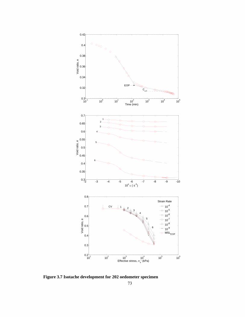
73
10-1 100 101 102 103 104 1050.3
0.32
0.34
0.36
0.38
0.4
0.42
Time (min)
Void
ratio
, e
Cαe
EOP
-10-9-8-7-6-5-4-3-20.3
0.35
0.4
0.45
0.5
0.55
0.6
0.65
0.7
Voi
d ra
tio, e
10x ε ( s-1)
12
3
4
5
6
101
102
103
104
105
1060.2
0.3
0.4
0.5
0.6
0.7
0.8
Effective stress, σv' (kPa)
Voi
d ra
tio, e
10-4
10-5
10-6
10-7
10-8
10-9
MSLEOP
1CV3
2
4
5
6
Figure 3.7 Isotache development for 202 oedometer specimen
Strain Rate
10-4
10-5
10-6
10-7
10-8
10-9
MSLEOP

74
10-3
10-2
10-1
100
101
102-30
-25
-20
-15
-10
-5
0
5
Normalized effective stress, σv'/σp'
Verti
cal s
train
, εv (%
)
crs (1.64x10⁻⁶s-1)crs (1.46x10⁻⁷s-1)MSL dia=16.9 (~10-6 s-1)MSL dia=25.0 (~10-7s-1)
10-3
10-2
10-1
100
101
102-30
-25
-20
-15
-10
-5
0
5
Normalized effective stress, σv'/σp'
Verti
cal s
train
, εv (%
)
crs (1.4x10⁻⁶s-1)crs (1.51x10⁻⁷s-1)MSL dia=16.9 mm (~10-6 to 10-7 s-1))MSL dia=25.0 mm (~10-6 to 10-7 s-1))
Figure 3.8 Comparison of MSL oedometer and CRS tests conducted (a) core 169 (41.75-
43.25m) and (b) core 202 (90.5-91.95m).

75
10-3
10-2
10-1
100
101
102-35
-30
-25
-20
-15
-10
-5
0
5
Normalized effective stress, σv'/σp' (kPa)
Ver
tical
stra
in, ε
v (%)
169us177us185us189us202us169s177s185s198s202s169crs (1.64x10⁻⁶ s-1)169crs (1.46x10⁻⁷ s-1)202crs (1.4x10⁻⁶ s-1)202crs (1.51x10⁻⁷ s-1)
Figure 3.9 Comparison of all oedometer and CRS tests conducted
10-3
10-2
10-1
100
101
1020
0.05
0.1
0.15
0.2
0.25
0.3
0.35
0.4
0.45
0.5
Normalized effective stress, σv'/σp'
Cc* =
Δe
/ Δlo
g σ
169us177us185us189us202us169s177s185s198s202s
(a)

76
10-3
10-2
10-1
100
101
1020
0.002
0.004
0.006
0.008
0.01
0.012
0.014
0.016
0.018
Normalized effective stress, σv'/σp' (kPa)
Cαe
= Δ
e / Δ
log
t
169us177us185us189us202us169s177s185s198s202s
(b)
Figure 3.10 Relationship between Cc* and Cαe and effective stress for all oedometer tests.
0 0.5 1 1.50
0.005
0.01
0.015
0.02
0.025
0.03
0.035
0.04
0.045
←Cαe / Cc = 0.03
Cc* = Δe / Δlog σ'
Cαe
= Δ
e / Δ
log
t
BearpawSt Hilaire Clay (Mesri et al., 1995)
Figure 3.11 Relationship between Cc*
and Cαe.

77
10-9
10-8
10-7
10-6
10-5
10-40.5
1
1.5
ε(s-1)
σp'/σ
p'(ε =
10-7
)
oedometercrs
Figure 3.12 Change in preconsolidation pressure with change in strain rate.
10-1
100
101
102
103
104
1050.4
0.42
0.44
0.46
0.48
0.5
0.52
0.54
0.56
Time (min)
Voi
d ra
tio, e
Cαe
Figure 3.13 Typical oedometer unloading increment.
(ε=1
0-7 s
-1)

78
10-3
10-2
10-1
100-0.1
-0.05
0
0.05
0.1
0.15
0.2
0.25
0.3
0.35
0.4
Normalized effective stress, σv'/σvmax' (kPa)
Cs* =
Δe
/ Δlo
g σ
169us177us185us189us202us169s177s185s198s202s
(a)
10-3
10-2
10-1
100-0.04
-0.035
-0.03
-0.025
-0.02
-0.015
-0.01
-0.005
0
0.005
0.01
Normalized effective stress, σv'/σvmax' (kPa)
Cαe
= Δ
e / Δ
log
t
169us177us185us189us202us169s177s185s198s202s
(b)
Figure 3.14 Cs* and Cαe versus effective stress for all oedometer tests.

79
0 0.1 0.2 0.3 0.4 0.5-0.03
-0.02
-0.01
0
0.01
0.02
0.03
0.04
Cc* and Cs
*= Δe / Δlog σ'
Cαe
= Δ
e / Δ
log
t
compressionswelling
Cαe / Cc
* = 0.03
Cαe / Cs
* =- 0.03
Figure 3.15 Relationship between Cc*
, Cs* and Cαe for all oedometer tests conducted.

80
Chapter 4
Examination of the swell behaviour of stiff natural clay
4.1 Introduction
Expansive or swelling soils are found throughout the world. The propensity of swelling
soils to undergo large volume changes driven by increases in moisture content under constant
stress causes damage to infrastructure measured in the billions of dollars every year (Keller,
2000; Puppala and Cerato, 2009). This places many additional geotechnical design challenges and
constraints on structures founded on these materials.
Due to the high costs of obtaining quality undisturbed samples and the sheer difficulty in
working with very stiff clay, there have been a few such studies conducted on undisturbed
samples (Hossain et al, 1997; Al Rawas et al, 1998). Most of the work conducted on natural clay
material is in the form of reconstituted and compacted samples which removes natural
heterogeneities, and the associated anisotropy that the sample has undergone during its history
(Sridharan and Gurtug, 2004; Basma et al, 1995; Al-Shamrani and Al Mhaidib, 2000; Romero,
1999).
Bjerrum (1967) observed that clay structure plays an important role in the observed swell
behaviour of the material. It was seen that in situ water contents in clay shale from southern
Saskatchewan were lower than rebounded remoulded clay from the lab. This was attributed to the
effect of structure and diagentic bonds in the clay. In contrast, Peterson and Peters (1963) found
that laboratory tests on clay shale in southern Saskatchewan used to determine swell
characteristic do not provide good correlation with observed field behaviour. It was seen that

81
swelling in-situ was much larger than predicted from laboratory consolidation tests suggesting
structure is not the only influential factor.
Siemens and Blatz (2009) showed that swell behaviour is heavily influenced by the
applied boundary conditions. These boundary conditions dictate the soils ability to undergo
changes in porosity and structure which affect the overall swelling ability of the material. A
swelling soil under constant volume or confined conditions will maintain its porosity during
water uptake, whereas a soil under constant stress conditions has the ability to increase its
porosity and thus change the hydraulic conductivity of the surrounding flow system. The ability
to accurately predict swell behaviour from laboratory testing is a challenge as traditional swell
pressure measurements are conducted in a one-dimensional apparatus where the samples are
rigidly confined. To accurately predict the amount of swelling a material will achieve in the field
requires representing the in-situ boundary conditions in the laboratory which is not possible with
traditional one-dimensional swell pressure measurements.
Figure 4.1 illustrates different types of boundary conditions that a sample may undergo.
The boundary conditions range from constant mean stress (CMS) to constant volume (CV) with
an intermediate spring-type boundary condition that incorporates displacements and increase in
stress. Work conducted by Siemens and Blatz (2009) on an engineered material (BSB), consisting
of 50 % sand and 50 % bentonite by mass, found that a unique Swell Equilibrium Limit (SEL)
exists for this material defined as the limit to volume expansion and confining stress that occurs
during water infiltration under controlled boundary conditions. The SEL provides a unifying
framework for the prediction of swell behaviour of the material and increases understanding of
swelling materials under wetting conditions.
The following work presents a two phased approach to assessing the swelling behaviour
of undisturbed natural clay samples from the Bearpaw Formation in southern Saskatchewan. In

82
addition to a variety of traditional one dimensional swell pressure tests, a series of specialized
triaxial swell tests were conducted under two controlled boundary conditions, constant volume
and constant mean stress, to assess the three dimensional swell behaviour of a natural material.
4.2 Background
4.2.1 Clay Mineralogy
Mineralogy is one of the dominant factors that control the size, shape, physical and
chemical properties of soil particles (Mitchell, 1993). In expansive soils, the swelling behaviour is
directly attributed to the clay mineralogy, in particular, the presence of montmorillonite. The
basic structural units of clay minerals are the silica tetrahedron and the aluminum or magnesium
octahedron which combine to form sheet structures as seen in Figure 4.2. Clay minerals are
formed by stacking combinations of these sheet structures with different forms of bonding
between the combined sheets (Craig, 1997). Montmorillonite is formed by combining two silica
tetrahedrons with one aluminum or magnesium octahedron. These combined sheets are bonded
weakly by water molecules and exchangeable cations as see in Figure 4.2. Isomorphous
substitution of magnesium for the aluminum in the octahedral sheet results in a net negative
charge on the clay surface. To balance this negative charge, cations are attracted to the clay
particle surface. At the same time the cations are being attracted to the particle surface they try to
diffuse away from one another due to their thermal energy (Craig, 1997). This creates a dispersed
layer away from the clay particles called the diffused double layer (DDL). The DDL has an
overall neutral charge due to the balance of positive and negative charges within the layer.
Thickness of the DDL is dependent on the valence of the cations, the concentration of the cations,
the charge of the cations and temperature (Mitchell, 1993).
The replacement of cations with water molecules within the diffuse double layer results
in the swelling behaviour of montmorillonite. Due to their dipolar nature, water molecules are

83
attracted to the clays negatively charged surfaces leading to expansion. By increasing the water
content of montmorillonite rich materials and thus increasing the availability of water in the DDL
leads to the increased expansion or swelling.
4.2.2 Swell Pressure Measurements
Traditionally, swell pressure measurements are one dimensional (1D) as they are
performed in a standard oedometer apparatus and thus confined radially. There are three methods
for measurement of swell pressure in an oedometer test, as outlined in ASTM D4546. The first
method involves loading the sample to a seating or in-situ pressure. Once vertical deformation
ceases the load is removed and the oedometer cell is filled with water allow the sample to swell.
Upon swelling the sample is recompressed back to the original seating or in-situ pressure. The
pressure at which this is achieved is considered the swell pressure. The second method is similar
however the seating or in-situ pressure is not removed prior to the addition of water. The sample
is allowed to swell under this seating or in-situ pressure. The sample is again recompressed until
the initial void ratio is achieved corresponding to the swell pressure. In the final method the
sample is loaded to a seating or in-situ pressure. The sample is then inundated with water while
additional load is added to prevent volume increase of the sample keeping it at a constant volume.
The final load applied to maintain a constant volume is noted as the swell pressure.
While the bulk of swell pressure measurements are conducted in this manner the
challenge lies in translating this swell pressure into predictions of volume change and practical
application. In nature soils do not swell in one dimension, resulting in the measured laboratory
swell pressure not providing an accurate reflection of the true material behaviour by under
predicting the swelling behaviour. Siemens and Blatz (2007) developed a new apparatus to
measure the volume change of a swelling soil under a variety of controlled boundary conditions
and thus relate the material behaviour to practical applications. Through this new controlled

84
testing it was found that there exists a limit to volume expansion and confining stress that occurs
during infiltration under controlled boundary conditions now referred to as the Swell Equilibrium
Limit (SEL). The SEL limit presented a framework for predicting behaviour of swelling soils
under general stress and volume state conditions for practical applications. Since the majority of
swell pressure measurements found throughout the literature are one dimensional they need to be
reinterpreted in order to correlate with the SEL and the new multi-dimensional swell tests. The
following section outlines the procedure by which this reinterpretation can be performed.
Work conducted by Gray et al. (1984) showed that conductivity in a swelling material is
a function of the clay dry density. Later Dixon et al. (2002) refined this concept and reported
swell pressure versus effective montmorillonite dry density (EMDD) for a variety of swelling
materials. EMDD is defined as the mass of bentonite divided by the volume of bentonite and
voids (thus excluding the volume taken up by non swelling materials). They found that as EMDD
increases the swell pressures increases as shown in Figure 4.3. This was later confined to just the
swelling portion of the material and resulting in the development of EMDD, a more
representative term for soil containing montmorillonite and whose behaviour is dominated by this
montmorillonite. This term is particularly useful in normalizing the behaviour of bentonites that
have varying montmorillonite content. EMDD is calculated as
⎥⎦
⎤⎢⎣
⎡ −−
−−
=
wn
dcm
ws
dc
dcm
ρGρ)ff(1
ρG)ρf(1
1
ρffEMDD 4.1
where:
fc = clay fraction,
fm = montmorillonite fraction of clay,
ρd = dry density,
ρw = density of water,
Gs = specific gravity of non-clay materials, and

85
Gn = specific gravity of clay materials
Siemens and Blatz (2009) and Siemens (2006) developed a procedure for converting 1D
swell pressure measurements to their equivalent equilibrium mean stress values in order to
compare with the triaxial swell tests measurements. The method and associated formula for this
conversion are outlined below.
To convert the one dimensional swell pressures obtained from the oedometer tests to an
equivalent end of test mean stress, and assumption of elasticity was made. From the generalized
form of Hooke’s law, elastic strain is defined as:
[ ])(E1
zyxx σσνσε +−= 4.2
where:
εx = strain in the x direction,
E = Young’s Modulus,
v = Poisson’s Ratio, and
σx,y,z = total stress in the x, y or z direction
However, for a one dimensional test, strain in the radial directions is equal to zero.
Similarly the horizontal stresses (in the x and y direction) are equal to the radial stress and the
vertical stress is equal to swell pressure simplifying equation 4.2 to
swellr P)1( ν
νσ−
= 4.3
where:
σr = radial stress, and
Pswell = swell pressure

86
Mean stress is defined as
3zyxp
σσσ ++= 4.4
where:
p = mean stress
σx,y,z = total stress in the x, y or z direction
In a one dimensional test the horizontal stress is equal to the radial stress and the vertical
stress is equal to swell pressure thereby simplifying the above equation to
32 rswell
equilP
pσ+
= 4.5
where:
pequil = equilibrium mean stress
By relating equations 4.3 and 4.5 to one another and assuming elastic behaviour of the
material we get the following expression for equilibrium mean stress (Pequil) in terms of Poisson’s
ratio and the swell pressure enabling the correlation of one dimensional swell pressure to three
dimensional mean stresses.
)1()1(
3 νν
−+
= swellequil
Pp 4.6
Using the above equation, one dimensional swell pressure can be converted to their 3D
equivalent using Poisson’s ratio for the material, enabling a direct comparison between one and
three dimensional swell pressure tests.

87
4.3 Materials and Methods
4.3.1 Material properties
The material used in the following laboratory tests were samples of the Cretaceous
Bearpaw clay-shale from southern Saskatchewan. The Upper Cretaceous Montana Group, in
particular the Bearpaw Formation, forms the bedrock surface over most of southern
Saskatchewan. The Bearpaw, the youngest formation of the Montana group overlying the Judith
River and Lea Park Formations, is a westward thinning wedge of predominately marine silty
clays and sands. The alternating sequence of silty clays and sands of the Bearpaw Formation were
deposited during the Campanian to early Maastrichtian and have been divided into 11 members
(Caldwell, 1968). Of the 11 members only two, the Ardkenneth and Snakebite Members, are
commonly seen in Saskatchewan. The Ardkenneth Member is a non-calcareous marine, very fine
– to fine grained sand and silt, and the overlying Snakebite Member is composed of non-
calcareous marine silt and clay. The Bearpaw Formation was deposited at a slow rate in relatively
quiet waters. Volcanic activity in south-western Montana occurred at various times during the
deposition of the Bearpaw Formation resulting in the layers of volcanic ash within the
sedimentary sequence (Scott & Brooker, 1968). During construction of the Gardiner Dam in
southern Saskatchewan Peterson (1954) found that the Bearpaw Formation could be divided into
three zones, an upper, middle and lower zone based on its structure and water content. The upper
zone was soft with high water content ranging from 29-36 % that contained many slickensides
and joint planes. The lower zone consisted of uniform, hard shale that had limited number of
slickensides and joints with water contents ranging from 20-27 %. The middle zone defined the
transition between the upper to lower zones, contained numerous fractures and exhibited water
contents ranging from 25-31 %.

88
Core samples were collected at a field site approximately 160 km south of Saskatoon
over 50 m interval. Commencing at 42 m below ground surface, core samples were taken every 6
m to a maximum depth of 92 m. Liquid and plastic limits range from 99 to 149% and 23 to 29%
over the entire sampled interval. Average water content and degree of saturation range from 19 to
30% and 90 to 98%, respectively. Average grain size over the entire sampled interval is 7% sand,
54% silt and 39% clay however local variation in the individual cores samples. Montmorillonite
content of the Bearpaw was found to be 71.6% by (Bryne & Farvolden, 1959). While in situ, the
Bearpaw is fully saturated with a water table surface sitting an average of 40 m above the
sampled area.
4.3.2 Test procedure and apparatus
The testing program for this work was divided into two phases. The first phase consisted
of conducting a series of one dimensional swell tests performed both in oedometers and constant
rate of strain test apparatuses related to other research areas of the thesis. These tests were
conducted on a number of different cores samples at varying depths as shown in Table 4.1. A
collection of over 24 tests were conducted. The variability of void ratios in specimens from the
same core sample, seen in Table 4.1, highlights the difficulty in measuring the void ratio in very
small specimens.
The second phase of the testing program consisted of four triaxial swell tests. The
apparatus used for this phase of the testing was developed by Siemens and Blatz (2007), which
applies radial infiltration under controlled wetting conditions. A schematic of the triaxial cell used
is shown in Figure 4.4. Modifications to the original design included designing a new pedestal
base for the sample with additional water outlets to promote radial flow around the entire
geotextile. A schematic of the new base design is shown in Figure 4.5. Apart from the base
modifications and the removal of the Xeritron sensor from the testing equipment the apparatus

89
used is the same as described in Siemens (2006). A custom data acquisition and control system
previous described in Blatz et al. (2003); Siemens (2006) and Siemens and Blatz (2007) was used
for data collections during the testing program.
The swell tests were conducted in two stages, the first being isotropic compression where
the cell pressure or mean stress was raised to 200 or 400 kPa. Following isotropic compression
water infiltration commenced under the set boundary conditions. The two types of boundary
conditions used were constant volume (CV) and constant mean stress (CMS).
Core samples were trimmed to cylinders of approximately 50 mm in diameter and 100
mm in height with emphasis on minimizing disturbance to the specimen as much as possible.
Special care was taken in trimming the specimen as pre-existing fractures were found throughout
the sample. Once trimmed, a piece of filter paper was wrapped around the middle of the specimen
before the entire specimen was wrapped in a geotexile that covered both the top filter stone and
the water outlet from the base. Two Lucite discs were placed against the specimen end to
maintain radial flow and control the water infiltration. The face of the Lucite disc in contact with
the specimen was covered in plastic wrap secured by vacuum grease to reduce friction at the end
of the specimen and ensure a good seal between the disc and the sample. Figure 4.6 shows a
photograph of the specimen prior to it being wrapped with the geotextile. Once placed on the
triaxial cell, the specimen is covered in two membranes that were sealed with o-rings on the top
cap and base. Four Linear Variable Displacement Transformers (LVDTs) with a maximum range
of 5mm were used to measure radial displacements. The LVDTs were located at mid-height and
positioned at right angles to the specimen. The LVDTs were held in position by Lucite holders
attached to the cylinder frame rods. Small cut-outs were made in the geotextile allowing the
LVDTs to contact the specimen directly beneath the membrane to eliminate volume changes due
to the expansion and contraction of the geotextile. Axial measurements were made using a LVDT

90
with maximum range of 25mm. This LVDT was secured directly to the top cap. Figure 4.7
contains a photograph of the specimen in the triaxial apparatus.
During the isotropic compression portion of the test, the mean stress was raised to either
200 or 400 kPa as dictated by the testing matrix shown in Table 4.2. Following volume
equilibrium with the applied pressure, infiltration under controlled boundary conditions was
commenced. Water was introduced into the systems through pressurized burettes at 100 kPa for
all tests.
4.4 Test Results
4.4.1 One dimensional swell pressure tests
Over 24 one dimensional swell pressure tests were conducted on undisturbed core
samples. A total of four different sample sizes were tested (63.5 mm, 36.5 mm, 25.0 mm and 16.9
mm in diameter) over a range of depths. The tests were conducted in an oedometer apparatus or
in a constant rate of strain apparatus both under constant volume conditions. The resulting swell
pressure measurements are shown in Table 4.1. In most cases, as sample size decreases the
measured swell pressure increases (Figure 4.8) with the 63.5 mm and 36.5 mm diameter
specimens showing the lowest swell pressures. Since these specimen sizes are known to be
disturbed (Chapter 2) they are removed from further discussions. The swell pressure data is
plotted again in Figure 4.9 and Figure 4.10 versus initial gravimetric water content and void ratio
respectively. Specimens are grouped according to their originating sample cores. As expected, as
depth increases both the water content and void ratio of the samples decreases. Other trends
include as the void ratio and water content decrease the swell pressure increases with notable
scatter as shown in Figure 4.9 and Figure 4.10. The variation in the swell pressures highlights the
non-uniqueness of these types of measurements and the implications of sample size as well as

91
effect of disturbance since, historically, swell pressure measurements have been done on large
sized samples.
4.4.2 Constant Mean Stress Tests
Two three dimensional triaxial swell tests were conducted under constant isotropic mean
stress boundary conditions, one at 200 kPa and the other at 400 kPa. Results for the 200 kPa and
400 kPa tests are shown in Figure 4.11 and Figure 4.12 respectively with volume strain, mean
stress and water added over the duration of the test. Water pressure was maintained at 100 kPa in
the two tests.
For the first sample (169a) (41.75-42.35 mbgs), isotropic compression was conducted at a
mean stress of 200 kPa during which the sample was compressed (positive volume strain). Water
was added to the system after 1 day at which point the sample volume began to increase. Initially
the water uptake was increased quickly and then levelled off over time. The total volume of water
that was added to the sample was 10.25 mL which was determined from the change in mass
before and after the test. After a period of 22 days the volume strain had stabilized and only
limited water infiltration was occurring and the test ended. The total change in volume strain was
-2.08%.
During the second test (169c), isotropic compression was conducted at a mean stress of
400 kPa and lasted 3 days. Again, sample compression occurred during isotropic compression
followed by volume expansion once water infiltration commenced. Water uptake occurred rapidly
upon exposure to water then levelled off. The total volume of water added to the sample was 4.21
mL and the test was complete after 18 days. The total change in volume strain was -0.10%.

92
4.4.3 Constant Volume Tests
Two tests were conducted under the constant volume boundary conditions with a water
pressure of 100 kPa. During the constant volume tests, sample volume was controlled throughout
water infiltration by increasing the mean stress isotropically to prevent any volume change from
occurring as the sample takes in water. Results for the 200 kPa and 400 kPa tests are shown in
Figure 4.13 and Figure 4.14 respectively with volume strain, mean stress and water added over
the duration of the test.
During the first constant volume test (169b), isotropic compression was conducted at a
mean stress of 200 kPa and lasted for 1 day. Water infiltration was then initiated under constant
volume boundary conditions and the test was continued for a total of 22 days. The initial water
uptake was fairly gradual in comparison to the constant mean stress tests and then continued to
level off over time. The amount of water taken into the sample was 3.75 mL. The equilibrium
mean stress at the end of the test was 653 kPa and the change in volume strain was 1.23 %.
Isotropic compression was conducted at a mean stress of 400 kPa and lasted for 3 days
during the second constant volume test (169d). Electrical issues with the motorized control of the
cell pressure were encountered such that this was monitored manually at the beginning of the test.
This is reflected in the oscillating behaviour of the mean stress up to approximately 10 days into
the test after which the problem was rectified and a constant mean stress was maintained as seen
in Figure 4.14. This oscillation in the mean stress did not have an effect on the overall volume of
the sample however the apparent water movement in to and out of the sample did respond and
tended to mirror this oscillation. The oscillation in apparent water movement is not representative
of the specimen but of water moving into and out of the geotextile which is compressible. The
final volume of water uptake was determined by the change in mass over the tests and therefore
was not affected. The test was completed after 18 days with a total water uptake of 1.79 mL. The
equilibrium mean stress was 767 kPa and the final change in volume strain was 1.01%
93
One interesting trend seen in both the CV tests is that the mean stress reaches a peak
value, at the onset of water infiltration, and then decreases to its equilibrium mean stress. This
initial increase then decrease in mean stress is an indication of unsaturated yielding behaviour,
however the low mean stress at which it appears to be occurring is uncharacteristic of this stiff
material. During wetting, under constant volume conditions, suction of the sample will decrease
as mean stress increases. Upon yielding, suction in the sample continues to decrease to zero
however the mean stress starts to decrease. Tests conducted on Boom clay show that samples
under high suction can exhibit yielding at relatively low mean stress values (Alonso et al, 1999).
Although there is evidence of yielding, further testing with suction measurement is warranted
before final conclusions can be made.
4.4.4 Comparison of CMS and CV Results
Results for the four tests conducted are shown in Figure 4.15 to Figure 4.17 as mean
stress, volume strain and water added to specimen versus time. A summary of the end of test
values for all four tests can be found in Table 4.3. The plots of mean stress and volume strain
versus time highlight the differences between the two boundary conditions applied. The mean
stress remains constant throughout the CMS tests while in the CV tests the mean stress increases
to a maximum mean stress, coinciding with the start of the water infiltration phase of the test,
then levels off to its equilibrium mean stress for the duration of the test. The equilibrium mean
stress was higher for the 400 CV test in comparison to the 200 kPa CV test. Unlike the constant
volume of the CV tests, the CMS tests were allowed to change in volume as seen by the relatively
large change initially, corresponding to the water infiltration phase, then levelling off. Increasing
the pressure in the CMS tests also reduced the volume expansion as seen in comparing the 200
and 400 kPa CMS tests.

94
The amount of water uptake is greater in the CMS tests in comparison to the CV tests and
greater for the 200 kPa tests in comparison to the 400 kPa tests of the same boundary condition.
This trend highlights the influence and importance on the imposed boundary conditions on the
amount of swell achieved. Prior to the test, the potential for swell was equal in each of the
samples due to the clay particles and their ability to expand when given water. In the case of a
constant volume test, the specimen is not allowed to increase in volume not allowing the clays to
expand, however for the CMS boundary conditions the clay particles are allowed to expand up
until the point that the applied mean stress counteracted this expansion. Prior to the test all
samples were unsaturated due to unloading during sampling and thus all the specimens took on
water.
Figure 4.18 through Figure 4.20 highlight the anisotropic volume change behaviour of the
samples. The two CMS tests initially undergo compression followed by expansion. The 200 kPa
test expanded more in the axial direction (1.16%) in comparison to the radial direction (0.45%),
whereas the 400 kPa sample expanded virtually the same amount in both the axial and radial
directions of 0.1%. The constant volume tests also exhibit anisotropic behaviour with the samples
expanding axially and compressing in the radial direction. The 200 kPa CV test expanded 0.35%
and compressed 0.43% while the 400 kPa test expanded 0.56 % and compressed 0.22%.
At the end of each test the triaxial sample was divided in to six sections and gravimetric
water contents were performed on each section. The general trend showed the highest gravimetric
water content at the top of the sample followed by the bottom with the middle being the lowest
GWC. The overall difference in water content across the sample was less than 3 % in all tests.
Figure 4.21 shows GWC versus mean stress again highlighting the effects of the applied
boundary conditions as they limit the amount of water that can infiltrate into the sample. The two

95
CMS tests show the greatest change in volume and increase in water content in comparison to the
CV tests.
From the above results, it is clear that boundary conditions influence the swelling
behaviour of this natural clay during water infiltration. The volume expansion and increased
mean stress during liquid infiltration continue until the clay equilibrated with the set boundary
condition. This agrees with the findings discovered by Siemens and Blatz (2009) when using an
engineered Bentonite Sand Buffer (BSB) material.
4.5 Discussion
4.5.1 Development of Swell Equilibrium Limit
Siemens and Blatz (2009) developed a Swell Equilibrium Limit (SEL), defined as the
limit to volume expansion and mean stress exists during water infiltration under controlled
boundary conditions. The SEL enables the prediction of final stress and volume states from initial
conditions such as stress, water content, specific volume and applied boundary conditions. By
examining gravimetric water content and volume strain versus mean stress as shown in Figure
4.21 and Figure 4.22, a SEL is apparent. Although the variation in gravimetric water content is
slightly different for the 200 kPa CMS specimen Figure 4.22, shows that the specimens swell or
increase due to swell induced stresses up to a limit. The 200 kPa CMS test swells more than the
400 kPa CMS. At the same time the 400 kPa CV test achieves an equilibrium pressure that is
greater to the 200 kPa CV. The same data is plotted as specific volume versus mean stress in
Figure 4.23 with the initial specific volume of the specimens set to the core value as performed in
Chapter 2 to remove the effect of this initial offset. Again, a clear end of test swell equilibrium
limit can be seen. The swell equilibrium limit was generated by taking the end of test values for
each of the four tests and fitting an exponential curve through them as shown in Figure 4.24. This
relationship indicated that a limit to volume expansion does exist in natural material however the

96
variation in initial conditions could influence the nature of this curve suggesting that the SEL may
change with depth. Work conducted previously (Chapter 3) showed that there is a linear
relationship between Cs* and Cαe indicating that the swelling behaviour of the Bearpaw is rate
dependent. Therefore, although not examined during this investigation, the SEL will also be
strain rate dependent.
4.5.2 Re-interpretation of one dimensional swell pressure
Swell pressure measurements and EMDD values from Table 4.1 are shown in Figure 4.25
in conjunction with the distilled deionised water data from Dixon et al. (2002) and BSB data from
Siemens (2006). EMDD has been shown to allow normalization of material properties of swelling
behaviour as it removes the effect of non-swelling fractions. The one dimensional swell tests
conducted during this work show good agreement with the Dixon et al (2002) data and all lie
within an acceptable scatter range of the existing data. The Bearpaw triaxial data has also been
converted to an equivalent swelling pressure using Equation 4.6. Unlike the BSB data, the
Bearpaw swell measurements lie both on and above the DDW line. This difference highlights an
important distinction between engineered and natural materials. In particular the affect of
structure within the material is likely having a strong influence on the results. The natural
variation of index properties including clay and montmorillonite fractions will also have an effect
on the measured swell properties compared with engineered materials with constant
configurations. Capturing this inherent heterogeneity is a common issue when working with
natural materials and continues to pose challenges.
4.5.3 Comparison of laboratory swell tests
In order to compare the 1D swell pressure tests, conducted in the first phase of the testing
program with the three dimensional swell tests from the second phase, the 1D swell pressures
must be converted to equilibrium mean stresses. Swell pressures from Table 4.1 were converted

97
to their equilibrium mean stress values using Equation 4.6 and are shown in Figure 4.26. Initial
comparison between the two different testing methods show that the initial void ratio is having a
clear influence. In addition, the 1D results show a large degree of variation while the triaxial
results give a consistent framework. From the triaxial swell pressure tests it was seen that the
initial conditions of the samples heavily influence the swell behaviour and therefore grouping the
samples in to one data set is not reasonable as the initial conditions vary considerably over the 50
m sample interval. Figure 4.27 breaks down the test data in to the core intervals from which they
originated. The triaxial samples were taken from the 169 core and thus are grouped into this
category. It now becomes apparent that samples from individual cores appear to have their own
swell limits and that a unique SEL for all the tested samples is not supported. A more reasonable
approach is to develop SEL curves for each core similar to those shown in Figure 4.27 to
encompass the range of swell behaviour. Two SELs are plotted in Figure 4.27, one for the 169,
and 202 samples due to the large amount of tests conducted on each of those cored intervals. The
202 data also shows a lot of variation however based on the behaviour seen in the triaxial swell
tests, it is likely that at lower stresses these curves will become exponential as shown in Figure
4.27. The exponential trend of the curve at low stresses is supported by the swell measurements
conducted by Peterson and Peters (1963).
4.6 Conclusions
This chapter presents a two phased approach in assessing the swelling behaviour of
natural clay samples from the Bearpaw Formation in southern Saskatchewan. A combination of
1D swell pressure and specialized triaxial swell tests were conducted. The resultant testing
outlines some of the challenges in working with natural undisturbed clay materials in comparison
to engineered material.

98
Over 24 1D swell pressure tests were conducted on clay samples of varying sizes and
depths. It was seen that these swell pressure measurements are dependent on size, with smaller
samples yielding higher swell pressures. The effect of disturbance size which was investigated in
Chapter 2 is reflected in these swell pressure measurements as well. In addition to size effects,
there appears to be significant variation in the observed swell pressures with samples of the same
size and depth. This highlights the importance of multi-sample testing and suggests that the
traditional method of 1 or 2 swell pressure measurements being applied to an entire region may
not sufficient.
In addition to the applied boundary conditions, initial conditions such as void ratio and
clay content have a large influence on the amount of swell achieved. When working in natural
material these parameters can vary significantly and therefore careful attention must be made
when grouping samples of the same material into one data set. There was acceptable agreement
between the converted 1D swell pressure measurements with the triaxial tests, over the range of
stresses under which the testing occurred, giving support to this new swell pressure testing
method. A series of SELs which vary with depth were developed to reflect the varying initial
conditions of the individual core samples. These SELs show that swell potential increases with
increasing depth of sample. This is consistent with the findings of Peterson and Peters (1963)
where it was observed that the unweathered clay exhibited more swell potential than the
weathered samples. Compared with the 1D data, the triaxial tests give a large amount of data so
that more realistic conditions can be represented in the laboratory.

99
4.7 References
Alonso, E.E., Vaunat, J. and Gens, A. 1999. Modelling the mechanical behaviour of expansive clays. Engineering Geology, 54(2),173-183. Al-Rawas, A.A., Guba, I., and McGown, A. 1998. Geological and engineering characteristics of expansive soils and rocks in northern Oman. Engineering Geology, 50, 267–281 Al-Shamrani, M.A., and Al-Mhaidib, A.I. 2000. Swelling behaviour under oedometric and triaxial loading conditions. In Proceedings of GeoDenver 2000: Advances in Unsaturated Geotechnics, Denver, Colo., 5 August 2000. American Society of Civil Engineers, New York. pp. 344–360. Basma, A.A., Al-Homoud, A.S., Husein Malkawi, A. 1995. Laboratory assessment of swelling pressure of expansive soils. Applied Clay Science, 9, 355-368 Bjerrum, L. 1967. Progressive failure of slopes of overconsolidated plastic clay and clay shales. Proceedings of the American Society of Civil Engineers, Journal of the Soil Mechanics and Foundations Divisions, 93, 2–49. Blatz, J.A., Anderson, D.E.S., Graham J. and Siemens G.A. 2003. Evaluation of yielding in unsaturated clays using an automated triaxial apparatus with controlled suction. Invited Lecture. International Conference From Experimental Methods Towards Numerical Modeling of Unsaturated Soils, Bauhaus-Universität, Weimar, Germany, September 2003, 285-300. Bryne, P.J.S., and Farvolden, R.M. 1959. The clay mineralogy and chemistry of the Bearpaw Formation of southern Alberta. Research Council of Alberta, Geological Division, Bulletin 4. Caldwell, W.G.E. 1968. The Late Cretaceous Bearpaw Formation in the South Saskatchewan River valley. Saskatchewan Research Council, Geology Division, Report #5 Craig, R.F. 1997. Soil Mechanics, Sixth Edition. E & FN SPON, London. Dixon, D.A., Chandler, N.A., and Baumgartner, P. 2002. The influence of groundwater salinity and influences on the performance of potential backfill materials. In Proceedings of the 6th International Workshop on Design and Construction of Final Repositories, Backfilling in Radioactive Waste Disposal, Brussels, Belgium, 11–13 March 2002. ONDRAF/NIRAS, Brussels, Belgium. Transactions, Session IV, paper 9. Gray, M.N., Cheung, S.C.H., and Dixon, D.A. 1984. The influence of sand content on swelling pressures developed by statically compacted Na-bentonite. Atomic Energy of Canada Ltd., Mississauga, Ont. (Available from the Nuclear Waste Management Division, Ontario Power Generation, Toronto, Ont.) AECL report 7825. Hossain, D., Matsah, M.I., and Sadaqah, B. 1997. Swelling characteristics of Madinah clays Quarterly Journal of Engineering Geology, 30, 205-220. Keller, EA. 2008. Environmental geology, Eighth Edition. Prentice Hall. USA

100
Mitchell, J.K. 1993. Fundamentals of Soil Behavior, Wiley, New York, USA. Peterson, R. 1954. Studies of Bearpaw shale at a dam site in Saskatchewan, Proc. ASCE, New York, v.80, separate no. 476. Peterson, R. and Peters, N. 1963. Heave of spillway structures on clay shales. Canadian Geotechnical Journal, 1, 5-15. Puppala, A.J. and Cerato, A.B. (2009). Heave Distress Problems in Chemically-Treated Sulfate-Laden Materials. GeoStrata. Vol. 10, Issue 2, pp. 28-32. Romero, E., 1999. Characterisation and thermo-hydro-mechanical behaviour of unsaturated Boom-clay: an experimental study. Ph.D. Thesis, Universidad Politécnica de Cataluña, Barcelona. 405 pp. Scott, J.S. and Brooker, E.W. 1968. Geological and Engineering Aspects of Upper Cretaceous Shale in Western Canada. Geological Survey of Canada. Paper 66-37. Siemens, G.A. 2006. The influence of boundary conditions on the hydraulic-mechanical behaviour of an unsaturated swelling soil. Ph.D. thesis, Department of Civil Engineering, University of Manitoba, Winnipeg, Man. Siemens, G.A. and Blatz, J.A. 2007. A triaxial apparatus for applying liquid infiltration with controlled boundary conditions and internal suction measurement. Journal of Geotechnical and Geoenvironmental Engineering. 133(6): 748-752 Siemens, G.A. and Blatz, J.A. 2009. Evaluation of the influence of boundary confinement on the behaviour of unsaturated swelling clay soils. Canadian Geotechnical Journal, 46(3), 339–356 Sridharan, A., and Gurtug, Y. 2004. Swelling behaviour of compacted fine-grained soils. Engineering Geology, 72(1), 9–18.

101
Table 4.1 One dimensional swell pressure test results.
Sample Depth
(m)
Initial
Water
Content
Initial Void Ratio
Seating
Pressure
(kPa)
Swell
Pressure
(kPa) EMDD
169L 29.5 0.860 10 191 0.700 169M 30.2 0.874 58 240 0.691 169S 28 0.849 116 225 0.707 169US 28 0.849 137 374 0.707 169US_0008 28.5 0.712 106.1 699 0.723 169US_00008
41.90 – 42.43
28.9 0.917 163.5 166 0.722 177S 27.1 0.824 116 420 0.728 177US
54.7-54.78 23.6 0.751 132 301 0.692
181US 60.47-60.5 27 0.859 136 255 0.698
185L 23.5 0.757 10 242 0.717 185M 22.8 0.613 57 226 0.641 185S 22.3 0.724 114 487 0.688 185US_b
66.48-66.83
22.5 0.668 136 1068 0.808 189US 72.9-73 24.6 0.740 135 354 0.707 195US 25.4 0.823 135 237 0.881 195US_b
79.2-79.25 22.3 0.806 132 251 0.888
198S 20 0.594 116 700 0.796 198US 85-85.14 21.2 0.650 131 515 0.815 202L 19.9 0.667 10 263 0.710 202M 21.6 0.774 58 231 0.721 202S 20.2 0.675 63 429 0.895 202US 19.9 0.614 133 811 0.841 202US_0008 22.5 0.782 44 683 0.837 202US_00008
90.79-91.15
20.5 0.624 53 1410 0.795
Table 4.2 Triaxial swell testing matrix.
Isotropic compression level (kPa) Boundary condition applied
200 400
Constant Mean Stress (CMS) 169a 169c Constant Volume (CV) 169b 169d

102
Table 4.3 Summary of end of test triaxial swell pressure tests.
Test type
Volume
Change
(%)
Equilibrium
Mean Stress
(kPa)
Water
Uptake
(g)
Gravimetric
Water
Content
(%)
Bulk
Density
(Mg/m3)
Dry
Density
(Mg/m3)
Saturatio
n (%)
200 kPa – Constant Mean Stress
-2.08 210 10.25 29.4 1.95 1.51 98.1
400 kPa – Constant Mean Stress
-0.10 402 4.21 30.7 1.94 1.49 99.2
200 kPa – Constant Volume
1.23 653 3.75 31.3 1.91 1.46 97.1
400 kPa – Constant Volume
1.01 767 1.79 29.8 1.93 1.49 97.0
Figure 4.1 Infiltration boundary conditions and stress volume paths applied by laboratory
apparatus.

103
Figure 4.2 Formation of clay minerals and structure of montmorillonite (after Craig, 1997).

104
Effective montmorillonite dry density, EMDD (Mg/m3)
0.0 0.5 1.0 1.5 2.0
Swel
ling
pres
sure
(MPa
)
0.01
0.1
1
10
100DDW10 mg/L NaCl
100 mg/L NaCl350 mg/L NaCl
35-60 mg/L NaCl
Figure 4.3 Swell pressure measurements (after Dixon et al. 2002).
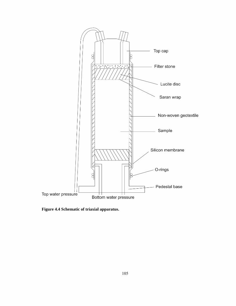
105
Figure 4.4 Schematic of triaxial apparatus.

106
Figure 4.5 Close up of pedestal base.
Figure 4.6 Photograph of specimen.
50 mm
100 mm

107
Figure 4.7 Photograph of specimen in triaxial cell.
Axial LVDT
Radial LVDT
Top Water Pressure

108
Void ratio, e
0.5 0.6 0.7 0.8 0.9 1.0
Sw
ell p
ress
ure
(kP
a)
0
500
1000
1500
2000
dia = 63.5 mm dia = 36.5 mmdia = 25.0 mm dia = 16.9 mmdia = 16.9 mm (CRS)
Figure 4.8 Effect of sample sizes on one-dimensional swell pressure measurements.
Gravimetric water content (%)
16 18 20 22 24 26 28 30 32
Sw
ell p
ress
ure
(kP
a)
0
250
500
750
1000
1250
1500
1750
2000169177185189198202 y=2.11E+06x-2.64
Figure 4.9 Gravimetric water content versus swell pressure for one dimensional swell tests,
ultra small sized samples only.

109
Void ratio, e
0.5 0.6 0.7 0.8 0.9 1.0
Sw
ell p
ress
ure
(kP
a)
0
250
500
750
1000
1250
1500
1750
2000169177185189198202 y= 1.73E+02x-3.02
Figure 4.10 Void ratio versus swell pressure for one dimensional swell tests, ultra small
sized samples only.
Time (days)
0 5 10 15 20 25
Mea
n st
ress
, p (1
00*k
Pa),
Volu
me
stra
in, ε
v (%
)
-3
-2
-1
0
1
2
3
Wat
er a
dded
to s
peci
men
(mL)
0
2
4
6
8
10
12
Volume strainMean stressWater added to specimen
Figure 4.11 200 kPa Constant mean stress test results: mean stress, volume strain and water
added to sample versus time (core 169, 41.75 – 43.25 mbgs).

110
Time (days)
0 5 10 15 20
Mea
n st
ress
, p (1
00*k
Pa),
Volu
me
stra
in, ε
v (%
)
-2
0
2
4
6
Wat
er a
dded
to s
peci
men
(mL)
0
2
4
6
8Volume strainMean stressWater added to specimen
Figure 4.12 400 kPa Constant mean stress test results: mean stress, volume strain and water
added to sample versus time (core 169, 41.75 – 43.25 mbgs).
Time (days)
0 5 10 15 20 25
Mea
n st
ress
, p (1
00*k
Pa),
Volu
me
stra
in, ε
v (%
)
0
2
4
6
8
10
Wat
er a
dded
to s
peci
men
(mL)
0
2
4
6
8
10
Volume strainMean stress Water added to specimen
Figure 4.13 200 kPa Constant volume test results: mean stress, volume strain and water
added to sample versus time (core 169, 41.75 – 43.25 mbgs).

111
Time (days)
0 5 10 15 20
Mea
n st
ress
, p (1
00*k
Pa),
Volu
me
stra
in, ε
v (%
)
0
2
4
6
8
10
Wat
er a
dded
to s
peci
men
(mL)
0
1
2
3
4
5
Volume strainMean stressWater added to specimen
Figure 4.14 400 kPa Constant volume test results: mean stress, volume strain and water
added to sample versus time (core 169, 41.75 – 43.25 mbgs).
Time (days)
0 5 10 15 20 25
Mea
n st
ress
, p (k
Pa)
0
200
400
600
800
1000
1200
200 kPa CMS400 kPa CMS200 kPa CV 400 kPa CV
Figure 4.15 Mean stress versus time for infiltration tests.

112
Time (days)
0 5 10 15 20 25
Volu
me
stra
in, ε
v (%
)
-3
-2
-1
0
1
2
200 kPa CMS400 kPa CMS200 kPa CV 400 kPa CV
Figure 4.16 Volume strain versus time for infiltration tests.
Time (days)
0 5 10 15 20 25
Wat
er a
dded
to s
peci
men
(mL)
0
2
4
6
8
10
12
14
16
200 kPa CMS400 kPa CMS200 kPa CV400 kPa CV
Figure 4.17 Water added to sample versus time for infiltration tests.

113
Volume strain, εv (%)
-2.5 -2.0 -1.5 -1.0 -0.5 0.0 0.5 1.0 1.5
Axia
l stra
in, ε
a (%
)
-2
-1
0
1
2
200 kPa CMS400 kPa CMS200 kPa CV 400 kPa CV
Figure 4.18 Axial strain versus volume strain for both CMS and CV tests.
Volume strain, εv (%)
-2.5 -2.0 -1.5 -1.0 -0.5 0.0 0.5 1.0 1.5
Rad
ial s
train
, εr (
%)
-1.0
-0.5
0.0
0.5
1.0
200 kPa CMS400 kPa CMS 200 kPa CV 400 kPa CV
Figure 4.19 Radial strain versus volume strain for CMS and CV tests conducted.

114
Radial strain, εr (%)
-1.5 -1.0 -0.5 0.0 0.5 1.0 1.5
Axi
al s
train
, εa (
%)
-1.5
-1.0
-0.5
0.0
0.5
1.0
1.5
200 kPa CMS 400 kPa CMS 200 kPa CV 400 kPa CV
Figure 4.20 Axial versus radial strain for CMS and CV tests conducted.
Mean stress, p (kPa)
0 200 400 600 800 1000 1200
Gra
vimet
ric w
ater
con
tent
(%)
25
27
29
31
33
35
200 kPa CMS400 kPa CMS200 kPa CV400 kPa CV
Figure 4.21 Gravimetric water content versus mean stress.

115
Mean stress, p (kPa)
0 200 400 600 800 1000 1200
Vol
ume
stra
in, ε
v (%
)-5
-4
-3
-2
-1
0
1
2
3
4
5
200 kPa CMS400 kPa CMS 200 kPa CV400 kPa CVSwell Equilibrium Limit
Figure 4.22 Volume strain versus mean stress.
Mean stress, p (kPa)
0 200 400 600 800 1000 1200
Spe
cific
vol
ume,
v
1.70
1.75
1.80
1.85
1.90
1.95
2.00200 kPa CMS400 kPa CMS200 kPa CV400 kPa CV Swell Equilibrium Limit
Figure 4.23 Specific volume versus mean stress.

116
End of test mean stress, p (kPa)
0 200 400 600 800 1000 1200
End
of t
est v
olum
e st
rain
, εv (
%)
-5
-4
-3
-2
-1
0
1
2
3
4
5
y = 1.467-9.28exp(-x/219.70)R2 = 0.98644
Figure 4.24 End of test volume strain versus end of test mean stress.
Effective montmorillonite dry density, EMDD (Mg/m3)
0.0 0.5 1.0 1.5 2.0
Sw
ellin
g pr
essu
re (M
Pa)
0.01
0.1
1
10
100DDWBearpaw (1D)
BSBBearpaw (Triaxial)
Figure 4.25 Swell pressure versus effective montmorillonite dry density(modified from
Dixon, 2002).
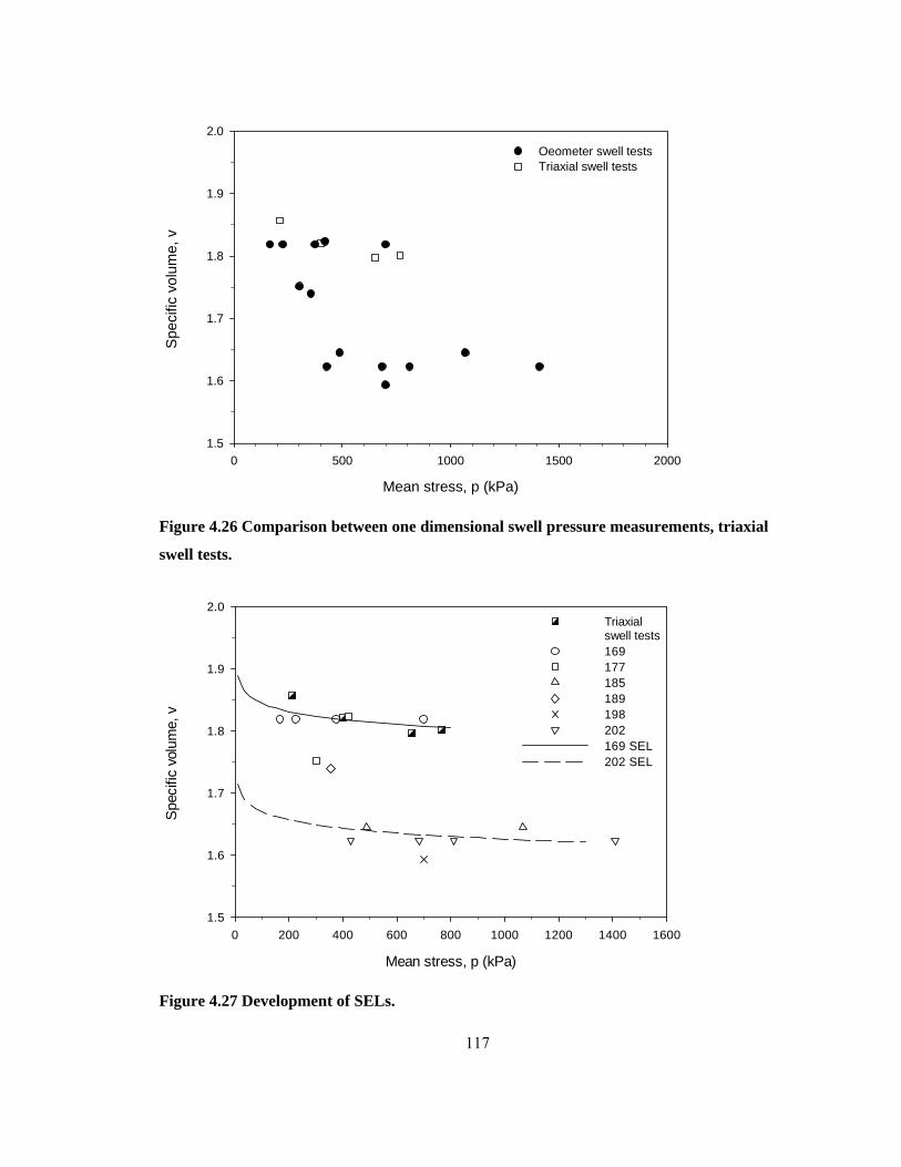
117
Mean stress, p (kPa)
0 500 1000 1500 2000
Spe
cific
vol
ume,
v
1.5
1.6
1.7
1.8
1.9
2.0Oeometer swell testsTriaxial swell tests
Figure 4.26 Comparison between one dimensional swell pressure measurements, triaxial
swell tests.
Mean stress, p (kPa)
0 200 400 600 800 1000 1200 1400 1600
Spec
ific
volu
me,
v
1.5
1.6
1.7
1.8
1.9
2.0Triaxial swell tests169177185189198202169 SEL202 SEL
Figure 4.27 Development of SELs.

118
Chapter 5
Constraining the age and deposition of glacial till using vertical stable
isotope profiles at two sites
5.1 Introduction
Throughout the Pleistocene, glaciers deposited thick successions of clay rich till over
Cretaceous deposits throughout southern Saskatchewan. Determining the glacial stratigraphy in
Saskatchewan can be quite challenging as there are very few unique characteristics found
amongst the different till deposits. The presence of oxidized zones and carbonate content are
generally the most useful tools to identify the different tills. There has been some work to suggest
that zinc and other trace elements can aid the above methods however they are not a standalone
method for identification (Schreiner, 1990). Additionally, several studies have used the
distribution of stable isotopes to provide information on groundwater flow, solute transport
mechanisms, hydraulic conductivity, and the timing of climatic and geologic events (Desaulniers
et al., 1981; Hendry, 1982; Simpkins and Bradbury, 1992; Remenda et al., 1996; Hendry and
Wassenaar, 1999; Hendry et al., 2000; Hendry et al., 2004).
Although the tills in southern Saskatchewan have been well characterized in the past,
using indicators such as carbonate content and the presence of oxidized zones (Christiansen, 1968
and Christiansen, 1992), there is evidence that the initial interpretation of some of the units may
be incorrect and require re-examination (Christiansen, 2005; Shaw & Hendry, 1998). Shaw and
Hendry (1998) found that 80 m of till previous thought have been deposited in the early
Wisconsin was actually that of the late Wisconsin Battleford Formation. Previous to this, the
Battleford Formation was thought to be less than 11 m in thickness throughout southern
Saskatchewan. The presence of such a large succession of the Battleford Formation has potential

119
implications to change the current interpretation of previously characterized tills within the area
and suggest further examination in the surrounding area is required.
In the study presented herein, single profiles of deuterium are modeled at two sites both
of which have till over a thick succession of the Cretaceous clayey silt Snakebite Member of the
Bearpaw Formation. The sites are ~10 km apart with essentially the same climate but different
landscape position and geometries. The objectives of this study were to (1) obtain till
geochemistry and pore water chemistry of till from a comparable site in terms of geological
history but that possesses a different geometry to the site described by Shaw & Hendry (1998),
and (2) use this data to model solute transport and investigate the age and type of till deposited.
During this work samples of the glacial till and underlying Cretaceous Bearpaw clay shale were
collected at one of the sites, over varying depth intervals up to a maximum depth of 90 m below
ground surface. The ability to obtain high quality samples from these depths is unique and not
often achieved due to cost and difficulty in sampling thus providing an enhanced vertical
examination of the material and the encompassing flow system. Analysis including carbonate and
zinc contents were performed on the till samples. Pore water was extracted from cores and
analyzed for both stables isotopes and selected anions providing a tracer profile with depth which
was subsequently modelled to aid in the age determination of the till at site. This method has been
successfully used by a number of researchers in the past (Hendry and Wassenaar, 1999; Gimmi et
al., 2007, Remenda et al., 1996).
5.2 Background
5.2.1 Groundwater flow
Flow through a porous medium is described by Darcy’s law. Darcy (1856) studied the
movement of water through a porous medium and found that the rate of flow through is
proportional to the difference in height of water and inversely proportional to the length of the

120
flow path as shown in Equation 5.1. The negative sign indicates that flow is in the direction of
decreasing head.
dldhK
AQq −== 5.1
where:
K = hydraulic conductivity
dldh
= hydraulic gradient
q = specific discharge
Q = discharge or flow rate
A = cross sectional area
Darcy’s law assumes a homogeneous, isotropic material, and both steady-state and
laminar flow. Specific discharge, q, is a macroscopic concept and does not take into account the
microscopic movement of fluid through the flow paths. Thus velocity calculations using this flow
rate and cross sectional area are fictitious as they assume flow occurs across the entire cross
section of the soil and not through individual flow paths. To account for these flow paths, the
effective porosity of the medium must be taken into account. Effective porosity is defined as the
porosity available for fluid flow and is always less than or equal to the total porosity of the
material. Specific discharge is divided by the effective porosity to give average linear
groundwater velocity as shown in Equation 5.2.
enqv = 5.2
where:
q= specific discharge
ne = effective porosity

121
5.2.2 Mass Transport Processes
Mass transport of solutes in groundwater is controlled by three mechanisms, advection,
dispersion and diffusion. Advection is the bulk transport of a solute in which is the moving
groundwater carries dissolved species with it. Dispersion is mixing that takes place during flow
and acts to dilute the solute and lower the concentration. Diffusion is movement of solutes from
areas of high concentration to areas of low concentration. Solute transport through a porous
medium is described by the advection-dispersion equation.
xCv
xCD
tC
x2
2
h∂∂
−∂∂
=∂∂
5.3
where:
C = solute concentration
vx = average ground water velocity (in the x-direction)
Dh = hydrodynamic dispersion
t = time
x = distance along flow path
Hydrodynamic dispersion, Dh, comprises both mechanical dispersion and molecular
diffusion and is expressed by:
exLh DvD +α= 5.4
where:
αL = longitudinal dispersivity
De = effective diffusion coefficient
As groundwater flow approaches zero the first term in Equation 5.4 also approaches zero
and becomes sufficiently small such that the effective diffusion coefficient is the more influential

122
mechanism for solution transport. In this case hydrodynamic dispersion is assumed to be equal to
the effective diffusion coefficient (Dh=De shows the range of specific discharge over which
hydrodynamic diffusion is either dominated by advective or diffusive migration.
5.2.3 Diffusion
The diffusion of a solute in water is described by Fick’s laws. Fick’s first law describes the flux
of a solute under steady state conditions.
xC
∂∂
−= oDJ 5.5
where:
J = mass flux of solute per unit area per unit time
Do = “free solution” diffusion coefficient
C = solute concentration
xC
∂∂
= concentration gradient.
Diffusion within porous media occurs at a slower rate than diffusion solely in water as it
can only occur through the pore openings and thus the pathways for migration are more tortuous.
The effective diffusion coefficient, De, is related to the free solution diffusion coefficient, Do, by
an empirically derived parameter tortuosity, τ:
oe D D τ= 5.6
where:
Do = “free solution” diffusion coefficient
τ =tortuosity factor
De = effective diffusion coefficient

123
Additionally, the reduced cross sectional area resulting from the presence of the soil
particles causes the diffusive mass fluxes to be less than in free solution. To account for the
tortuosity and reduced area that affect the rate of diffusion within a porous medium, a tortuosity
factor and the volumetric water content are added to Fick’s law to describe diffusion in soil as
shown in equation 5.7 (Shackelford and Daniel, 1991).
xC
∂∂
−= θeDJ 5.7
where:
θ = volumetric water content
τ =tortuosity factor
De = effective diffusion coefficient
To describe transient diffusion conditions, where the concentration changes over time,
Fick’s second law is applied. By assuming that the volumetric water content is constant through
time and space, this term is cancelled in the derivation of Fick’s second law leaving just effective
diffusion coefficient to be considered as shown in Equation 5.8. Generally it is the effective
diffusion coefficient that is measured in the laboratory and in the field (van der Kamp et al., 1996;
Hendry and Wassenaar, 1999; Remenda et al., 1996).
2
2
eDCxC
t ∂∂
=∂∂
5.8
where:
t∂∂C
= change in concentration with time
De = effective diffusion coefficient

124
5.2.4 Stable Isotopes of Oxygen and Hydrogen as Tracers
Isotopes of a particular element have the same atomic number but different atomic
weights and are categorized as either stable or radioactive. Stable isotopes are not subject to
radioactive decay processes but instead fractionate readily, due to having relatively large
differences in mass between two isotopes and have one isotope that is more abundant than the
other as shown in Table 5.1. Fractionation is defined as any process that causes the isotopic ratio
in particular phases or regions to differ from one another as a result of the mass difference
between the isotopes (Drever, 1982). Isotopic ratios of these elements are written as the ratio of
heavy to light isotope such as 18O/16O and 2H/H. These variations in isotopic abundances that
occur during fractionation are relatively small. Since relative difference in isotopic ratios can be
more precisely determined than absolute isotopic ratios these small relative difference in isotopic
ratio are reported as delta values in units of per mill (parts per thousand) as a ratio relative to a
standard shown in Equation 5.9. A positive δ value indicates that the ratio of the heavy to light
isotope is higher in the sample than in the standard and a negative value the opposite (Clark and
Fritz, 1997).
1000R
RR
standard
standardsample ×−
=δ 5.9
where:
δ = del (parts per thousand)
Rsample = isotopic ratio of the sample
Rstandard = isotopic ratio of the standard
5.2.4.1 Meteoric water
Meteoric water is water that has been part of the meteorological cycle (rain, snow, etc).
All surface waters (lakes, river, and glaciers) and some groundwater fall under the category of
meteoric water. The ocean is not considered meteoric although it continually receives meteoric
125
waters (Hoefs, 2004). During phase changes between a liquid and gas, the heavier isotopes
concentrate in the liquid phase and the lighter in the gas phase resulting from the fact that the
vapour pressure of water containing the light isotopes is greater than water containing the heavier
isotopes. Partitioning of the heavy and light isotopes is primarily dependent on the mean annual
temperature and the physical and geographical properties affecting the air mass in which
precipitation is generated. For all processes concerning evaporation and condensation of water the
hydrogen isotopes are fractionated in the same manner as the oxygen isotopes because of a
corresponding difference in vapour pressure. This relationship between oxygen and hydrogen
isotopes allows for a correlation between them in meteoric waters. Craig (1961) defined the
global meteoric water line (GMWL) to describe the linear relationship between δD and δ18O in
surface waters from around the world as shown in Figure 5.2. The GMWL is global in application
only and is an average of many local or regional meteoric water lines. These local meteoric water
lines have slightly different slopes and intercepts than the GMWL resulting from differences in
altitude, local climate and distance from the moisture source. There are number of physical and
chemical processes that can alter the isotopic ratio of meteoric waters causing them to fractionate
and deviate form the meteoric water line. Some of the common processes to affect meteoric water
and the resultant deviation from the meteoric water line is shown in Figure 5.3. VSMOW (Vienna
Standard mean Ocean Water) is the internationally accepted reference for both 18O and 2H in
water.
5.2.5 Stable isotopes and age determination of groundwater
Vertical stable isotope profile has been used in low permeability material successfully by
others to aid in the age determination of groundwater. As discussed earlier, partitioning of the
heavy and light isotopes of water are dependent on temperature and the air masses in which
evaporation and precipitation are occurring. During the last glaciation evaporated water enriched

126
in the lighter isotope, became stored in the ice sheets causing the ocean to become enriched in
heavy isotopes. As the light enriched and heavy isotope ice sheets melted, heavy isotopes were
removed resulting in precipitation that was more depleted than present day values due to the
storage of light isotopes in the ice sheets. Thus, glacial melt waters can be distinguished from
present day precipitation due to the depletion of heavy isotopes in the water. This difference in
isotopic ratios between precipitation during glaciation and that of present day precipitation can
then be traced and monitored in some current groundwater systems. In low permeability
groundwater systems typically dominated by diffusion, the rate the movement of water is
sufficiently slow that remnants of the glacial melt water are still present today. Through
examination of the current isotope distribution in the subsurface, estimates of groundwater age
can be achieved typically by modelling the measured profile and time it would take to develop it,
thereby allowing timing of the groundwater in the system to be achieved. Both Desaulniers et al.
(1981) and Remenda et al. (1996) used vertical 18O profiles to estimate the age of the
groundwater in two thick clay rich deposits from Ontario and Saskatchewan. In both instances the
18O profiles were enriched near ground surface becoming more depleted with depth. These 18O
concentration profiles were then simulated in a one dimensional transport model, using relevant
groundwater properties to estimate the time over which the measured profile took to develop.
Similarly, Hendry and Wassenaar (1999) modelled a vertical 2H profile across glacial till and
Cretaceous clay deposits in southern Saskatchewan. The resultant groundwater ages modelled by
Hendry and Wassenaar (1999) were then used to isolate the time period during which the till
material was deposited, and thus the formation to which it belonged. This finding was particularly
significant, as it revealed the Battleford Formation to be upwards of 80 m thick where it was
previously thought be less than 11m in thickness. As a result, the stratigraphy of the tills in the
region remains under question.

127
5.3 Geology of Southern Saskatchewan
In general, the geology in this region of southern Saskatchewan comprises a thick
succession of clayey glacial tills, from at least six glaciations, overlying Cretaceous clay shale
deposits (Figure 5.4). The glacial deposits have been divided into two groups, the younger
Saskatoon Group that overlies the Sutherland Group, based on the carbonate content and
stratigraphic position (Christiansen, 1992). The Saskatoon Group is subdivided into the Battleford
and Floral Formations on the basis of pre-consolidation pressures, structure, staining and
carbonate content. The Battleford Formation is typically softer than the Floral Formation, massive
and unstained and is often up to 80m thick. The Floral Formation contains over-consolidated,
jointed and stained tills that range in thickness from less than 1m to 71m. In some regions, the
Upper and Lower Floral Formation tills are separated by the Riddell Member, the oldest dated
stratigraphic unit. Radiocarbon ages of carbonaceous material between tills of the Floral and
Battleford Formations range form 38 000 ± 560 to 18 000 ± 450 years (Christiansen, 1971). The
Sutherland Group is divided into the Warman, Dundurn and Mennon Formations. The Warman
Formation ranges from 1 to 21 m thickness. The lower contact which is distinct and non-
conformable is marked locally by the top of the oxidized zone in the Dundurn Formation. The
Dundurn Formation is composed of till and stratified drift. Generally the Dundurn Formation has
more sand and gravel interbeds than other formations in the Sutherland Group. The Mennon
Formation ranges in thickness from less than 1 m to 31 m. The lower contact is conformable
where the upper proglacial unit of the Empress group is present and unconformable where part or
all of it is missing. Schreiner (1990) found that the Quaternary stratigraphy is a mirror image of
the Cretaceous bedrock sequence and that the till deposits resulted from progressive stripping of
the underlying bedrock. During this glacial stripping, Cretaceous shales were removed from the
Precambrian Shield and lower Cretaceous sandstones south of the shield. Schreiner (1990)
determined that the Keewatin ice centre was the main centre of ice accumulation for all the tills

128
except for that of the Dundurn Formation which could not be associated with a bedrock unit in
the Cretaceous sequence. It was suggested that the Dundurn Formation was derived from rocks
with higher carbonate content lying to the east by ice moving from a more easterly direction.
The Upper Cretaceous Montana Group, in particular the Bearpaw Formation, forms the
bedrock surface over much of this region. The Bearpaw, the youngest formation of the Montana
group (71-72 Ma), overlying the Judith River and Lea Park Formations, is a westward thinning
wedge of predominately marine silty clays and sands. The alternating sequence of silty clays and
sands of the Bearpaw Formation were deposited during the Campanian to early Maastrichtian and
have been divided into 11 members (Caldwell, 1968). The Snakebite Member is composed of
non-calcareous marine silt and clay and overlies the Ardkenneth Member, a non-calcareous
marine, very fine – to fine grained sand and silt. The Bearpaw Formation was deposited at a slow
rate in relatively quiet waters. Volcanic activity in south-western Montana occurred at various
times during the deposition of the Bearpaw Formation resulting in layers of volcanic ash within
the sedimentary sequence (Scott & Brooker, 1968).
5.4 Materials and Methods
5.4.1 Site Description
A field site, located roughly 160 km south of Saskatoon near the towns of Birsay and
Lucky Lake, was selected for the following investigation (Figure 5.5). The site, hereafter called
the Luck Lake site, consists of 30 m of glacial till, thought to be that of the Battleford and Floral
Formations, overlying approximately 90 m of the Snakebite member of the Bearpaw Formation.
The Luck Lake site is located adjacent to the Luck Lake Heritage Marsh, a Ducks Unlimited
project that is supplied water from Lake Diefenbaker by an underground pipeline. Prior to the
development of the marsh in 1987, Luck Lake was a large shallow saline lake, very typical of the
southern prairies and thus subjected to large variations in lake levels. Drilling at site was

129
conducted on two separate occasions. The first drilling was conducted in November, 2005 with
Probe Drilling using a hollow stem auger rig in which four 0.76 mm diameter Shelby tube
samples were collected in the till every 3 metres between 12 m and 21 m. The second
investigation was conducted in September 2006 with Saskatchewan Department of Highways
using a hydraulic rotary drill. Washed cuttings were taken during the entire length of the
borehole. The hole was cased to the till/clay contact to facilitate sampling over multiple days.
Three 0.6m long Shelby tubes were collected near the till/clay contact until the clay became
sufficiently stiff that the Shelby tubes would no longer penetrate the clay. Following this, nine
1.5m Denison core barrels were collected every 5 m between 42 and 92 m within the Bearpaw
Formation. A stratigraphic borehole log, including sample locations from all investigations, is
presented in Figure 5.6. Evidence of bentonite lenses, shell fragments and large concentration
layers were also observed during the investigation. Resistivity, spontaneous potential and gamma
logs were obtained before backfilling of the borehole took place and are shown Figure 5.7.
Further details of core sampling and preservation are given in Appendix E. In addition to the two
investigations above, dried samples collected during earlier investigations on site (Remenda,
1993) were used for subsequent analysis as part of this research.
Investigations prior to this study at the Luck Lake site, (Remenda, 1993) resulted in the
installation of six piezometers which were used during this study. Four wells were located in the
glacial till with the depth to screen at 3, 8, 12, 24 m. The remaining two wells were set in the clay,
one at the till/clay (32 m) and the other 42 m below ground surface.
5.4.2 Till and Clay Properties
5.4.2.1 Geochemistry
The atomic absorption method (Ross, 1986) was used to determine carbonate content of
the till from the Luck lake site. Weight percent measurements of calcium and magnesium were

130
obtained from work done previous on site (Remenda, 1993). These calcium and magnesium
values were then converted into equivalent amounts of calcite and dolomite using the method
described by Ross (1986). Total carbonate, measured as the total CO2 evolved, was then
determined and reported in mL CO2 per gram of sample. Calcite and dolomite are considered to
the dominate forms are carbonate minerals as no other appreciable amounts of carbonate bearing
minerals were found during a detailed mineralogical analysis on southern Saskatchewan tills
(Ross, 1986). Weathering, such as oxidization of iron and magnesium and precipitation of
gypsum, occurs during interglacial periods and has a slight influence on the total carbonate
content. The gypsum that is precipitated during weathering contains calcium such that when the
calcium content of the till is determined, the calcium present in the gypsum in included in the
overall calcium in the till which slightly affects the total carbonate content measured. However,
the weight percent of calcium in the gypsum was found to be insufficient relative to the amount
of calcium in the till and therefore is not considered a significant factor in carbonate content
evaluation (Fortin et al., 1991)
Zinc analysis was performed on the dried till samples. These samples were crushed and
sieved through a 180 µm sieve before being sent to Activation Laboratories in Ancaster Ontario
for analysis. Zinc was determined using the Aqua Regia - ICP method.
5.4.2.2 Physical Properties
Grain size analysis was performed on the cored clay according to ASTM (2000c).
Atterberg limits of the till and clay were conducted used the dry preparation method as outlined in
ASTM D-4318 (ASTM, 2000a). Due to the limited core samples acquired in the till, density and
porosity measurements were only taken in the clay. The bulk density of the samples was obtained
by taking multiple measurements of both the diameter and length of cut core samples to
determine the dimensions of each sample. The bulk density was then defined as the ratio between

131
total mass to total volume. Subsequent water content measurements were used to determine the
dry density of the samples and the porosity.
5.4.3 Pore water extraction
Squeezing was used to extract pore water from each of the cored samples. The squeezing
apparatus consisted of an Enerpac 25 ton capacity hydraulic cylinder (Rc-256), that was
controlled with an Enerpac P39 10,000 psi rated hand pump and hose (Figure 5.8). An Enerpac
G4088L dial gauge was used to measure the pressure applied to hydraulic cylinder. The Enerpac
cylinder was attached to threaded metal frame and the frame secured to the work bench via
clamps. Samples were placed in a machined steel cylinder during squeezing. A bottom outlet port
in the base of the cylinder was used for pore fluid collection. Metal screening, topped with filter
paper was used to cover the outlet port and minimize sediment collection during squeezing.
Tubing and a glass vial were attached to the outlet port on the outer base of the cylinder for water
collection. The apparatus is shown in Figure 5.9 and Figure 5.10. Samples averaging 7 cm in
length were trimmed to fit snugly and placed in the steel cylinder. These samples were then
loaded incrementally up to a maximum load of 27650 kPa. The rate of loading varied from 1722
kPa every 30 min to 1378 kPa every 60 min. Once water started to be expelled from the sample,
generally around 24115 kPa to 27650 kPa due to the small volume of water initially present in the
sample, the pressure was held constant over the duration of water collection. Where possible,
water collection was completed within 24 hours. When adequate water collection was not
achieved in 24 hours, sample vials were sealed from atmosphere to minimize evaporation effects.
Once full, the glass vials containing the expelled pore water were sealed and placed in a cold
room or fridge until required for subsequent analysis. On average each sample yielded 5 mL of
fluid.

132
5.4.4 Water and Stable Isotope Analysis
Extracted pore water and water well samples were analyzed for deuterium, 2H or D, and
oxygen-18, 18O, in the Queen's Facility for Isotope Research University and anions were analyzed
at the Queen’s Analytical Services Unit (ASU). Hydrogen was analyzed using ThermoQuest
Finnigan H/Device, interfaced to a ThermoFinnigan Mat 252 Mass Spectrometer. Each water
sample was vaporized over chromium metal at 850oC producing hydrogen gas that was analyzed
in the mass spectrometer. Oxygen isotopes were measured by calibrating the water sample with
CO2 in He gas in a Gas bench and analyzed the CO2 equilibrated water with Thermo Finnigan
Delta Plus XP Mass spectrometer. Results were reported in del notation relative to VSMOW with
an accuracy of ± 1per mil for δD and ± 0.3 per mill for δ18O.
5.5 Test Results
5.5.1 Index Properties
Index properties, including Atterberg limits, density and porosity of the clay and sections
of the till are plotted in Figure 5.11. Liquid and plastic limits in the till range from 29 to 38% and
13 to 16% with an average water content of 17%. In the clay, liquid and plastic limits range from
99 to 149% and 23 to 29%, respectively with an average water content of 26%. The till clay
boundary is marked by as distinct change in properties, in particular the liquid limit. Natural
water content values are higher than the plastic limit for the till and upper clay samples. Below 60
m the water content is less than the plastic limit. Dry density and bulk density measurements
ranged from 1.35 to 1.73 Mg/m3 and 1.89 to 2.09 Mg/m3, respectively both increasing with depth.
With the exception of the upper most clay samples, the porosity of the clay is essentially constant
with depth. Plasticity of the till ranges from medium to low, whereas the clay has high plasticity
as seen in Figure 5.12 as denoted by the Unified Soil Classification System (USCS) (ASTM,
2000b). Sauer et al (1993) found that plasticity values varied between tills of the Saskatoon and

133
Sutherland Group tills. The till at this site shows plasticity ranges consistent with that of the
Saskatoon Group tills. The average grain size (over the sampled interval) is 7% sand, 54% silt
and 39% clay with local variation in the individual cores samples.
5.5.2 Hydrogeology
During both site visits water levels in the six existing piezometers were measured as
shown in Table 5.2. Water table elevations ranged from 2.0 to 2.3 m below ground surface over
the course of the two visits with an average gradient in the till of 0.014 and 0.21 in the clay.
Water level readings in piezometer 90-01, installed 13m into the top of the clay, maintained a
level lower than the adjacent piezometers installed in the overlying till. This decreased water
level could be a result of a downward gradient or underpressuring within the clay due to erosional
unloading of overburden or isostatic rebound. Overpressuring and underpressuring has been
found to occur in a variety of low permeability deposits throughout the Alberta Basin as a result
of glaciation, erosion or unloading producing abnormal fluid pressures within these deposits
(Bekele et al., 2003; Neuzil,1993; Wilson et al., 2003). The complete reversal of flow systems,
due to glacial loading and unloading has been found to significantly re-organize present day
groundwater systems (Grasby and Chen, 2005). In this area, the hydraulic head of the underlying
Ardkenneth Member aquifer is roughly 50 mbgs and the regional groundwater flow has been
found to be downward (van der Kamp and Jaworski, 1989). Therefore, the lower water pressure
in the clay is believed to be that of a downward gradient. While it is possible that low water
pressures within the clay is a result of underpressuring, a more detailed investigation to obtain
further measurements within the clay would be necessary.
Previous work conducted on site (Remenda, 1993) produced similar results however not
all piezometers had fully recovered following installation. Average downward linear groundwater
velocities at the Luck Lake site have been measured at values up to 3 m per 10,000 years

134
(Remenda 1993). Slug tests performed following piezometer installation on site yielded hydraulic
conductivity values in the till that range from 4x10⁻¹⁰ m/s to 3x10-11 m/s. In addition, hydraulic
conductivity values were obtained from over 35 consolidation tests, conducted on samples of the
Bearpaw Formation as part of additional investigations on site (Chapter 2). Figure 5.13 shows the
results from the oedometer tests showing a linear relationship between hydraulic conductivity and
void ratio. Field void ratio measurements range on the order of 0.6 correspond to hydraulic
conductivity values of 10-12 m/s. Similar results were also reported by Shaw and Hendry (1998) at
the King site.
5.5.3 Till geochemistry
The results of carbonate and zinc analyses are presented in Table 5.3 and Figure 5.14.
Carbonate content increases slightly with depth corresponding with the change from oxidized to
unoxidized till and has a mean value of 26.9 mL CO2/g within the till. The zinc content is
consistent with depth with an average value of 70.7 ppm. The till-clay boundary is marked by a
distinct change in both the zinc and carbonate contents. Christiansen (1968) used carbonate
content to distinguish among the till formations and average values are shown. Based solely on
carbonate content it appears the till at the Luck Lake site fits best into the Battleford Formation or
the Dundurn Formation. However due to the variation in carbonate content within each
formation, this is not a conclusive method for determining the till stratigraphy however it can
provide a useful tool for distinguishing Saskatchewan tills. Schreiner (1990) found that trace
elements such zinc could be used as additional tool in distinguishing the till units and
complement the use of carbonate content. Table 5.5 gives Schreiner’s results for Zn. Despite the
variation in the zinc results seen in Table 5.5, it appears the till at this field site falls within the
Saskatoon Group tills likely the Battleford or the lower Floral Formations. Again, due to the
variation found in the results, it is not conclusive. Utilizing both the carbonate and zinc results it

135
can be determined that the till is likely a Saskatoon Group till however distinguishing between the
Floral and Battleford Formation is not possible with these two identification techniques. The
presence of oxidized zones is also a critical tool in the delineation of the tills stratigraphy as these
zones act as an unconformity and based on the placement of this oxidized zones different
stratigraphic units can be delineated. Oxidized zones are the most common indicator of
weathering and thus the top of an oxidized zone represents an erosion surface or a period of non-
deposition. Due to the presence of an oxidized zone above 18 m at the Luck Lake site, it was
previously thought that the till on site belonged to the Floral Formation as the younger Battleford
Formation was characterized as being massive and unstained. Results from the carbonate and zinc
contents do not dispute this but introduce the possibility that it may be the Battleford Formation.
Sauer and Christiansen (1991) saw that the Battleford Formation can be seen to be oxidized when
located above the water table. Although water levels at the Luck Lake site have been relatively
stable over the studied time period, prior to 1987 and the development of the Luck Lake Heritage
Marsh, Luck Lake was subjected to large fluctuation in water levels. These fluctuations likely
influenced the surrounding water table and as such the presence of the oxidized zone at the luck
lake site could be attributed to local fluctuations in the water table. Shaw and Hendry (1998)
found that among 80 m of the Battleford Formation an oxidized section was present, likely due to
the re-deposition of material during glaciation. Additionally, at a site near Saskatoon the
Battleford Formation was divided into an upper and lower till suggesting the possibly of two
depositional periods of the Battleford Formation (Sauer and Christiansen, 1991).
5.5.4 Stable isotope analysis
Pore water samples were extracted from core samples from both the till and clay by the
method of squeezing as described earlier. The results for the deuterium and oxygen-18 analysis
are shown in Figure 5.15. The extensive vertical distribution of stable isotopes to a depth of 90 m

136
is unique in itself as extraction and analysis of water samples up to this depth is vary rare due to
the cost and difficulty in sample collection. The δD and δ18O profiles decrease in value from -
155‰ and -20‰ around 8 m below ground surface to -171‰ and -22‰ at 25 m. The profiles
then increase across the till clay boundary to until reaching constant values of -142‰ and -18‰
at around 70m. This profile is consistent with results obtained by others in low permeability
material that are dominated by diffusion (Hendry and Wassenaar, 1999; Remenda et al., 1994;
Remenda et al., 1996; Hendry et al, 2004). The values of δD and δ18O near ground surface and
within the upper oxidized zone of the till reflect the input of modern day precipitation of -136‰
and -17‰. The zone of mixing with modern day precipitation is confined to the upper weathered
zone as supported by previous measurements of tritium on site (Remenda, 1993) which show
detectable levels above 12m but were not detectable at 24 m. The depleted values near the base
of the till, just above the till/clay boundary, reflect values consistent with reported values of
glacial melt water (Remenda et all., 1994, Hendry and Wassenaar, 1999). Across the till/clay
boundary the profile exhibits a characteristic diffusion profile representing an marked change in
the pore water chemistry between the formations. The values at depth are in agreement with
measured values from the underlying aquifer (Cey et al, 2000; Hendry and Wassenaar, 1999).
The method of squeezing (Patterson et al, 1978; Entwisle and Reeder, 1993) was selected
as the best way to extract pore water in this case. Although alternative techniques such as
diffusion, direct CO2 equilibration, vacuum distillation, centrifugation have been found useful by
other researchers (Kelln et al, 2001; Koehler et al, 2000; van der Kamp et al. 1996; Sacchi et al.
2001), squeezing was deemed suitable for this application. There has been speculation as to
whether the method of squeezing results in fractionation of the pore water however there has not
been conclusive evidence shown in either direction. As seen in Figure 5.16 fractionation of the

137
deuterium and oxygen-18 was not evident as the data lie along the local meteoric water line for
Saskatoon.
5.5.5 Anion Analyses
Due to the limited amount of pore water extracted from the samples, in addition to
maximizing the information obtained, sulphate and chloride were selected as the anions to be
analyzed. The results of these anions with depth can be seen in Figure 5.17. The chloride profiles
can be broken up into various sections and has a similar diffusion dominated profile to that of the
isotopes. The top part of the profile shows lower chloride values increasing to a peak
concentration of 195 mg/L at 12.5 m. This peak was not reflected in the isotope profiles but
suggests a source input or concentration of chloride at this depth. Similar results were seen by
Hendry et al. (2000) and were attributed to a concentration of chloride within sand streaks. Sand
streaks were not conclusively seen at this depth however an increase in moisture content was
noted during both drilling investigation suggesting an area of increased permeability. Above 8 m
it is expected that the chloride values continues to decrease due to the infiltration of precipitation
containing minimal amounts of chloride. The lack of shallow samples obtained during this study
can not confirm this however previous sampling on site and sampling result from the King site
support this (Remenda, 1993; Hendry et al, 2000). Below 12.5 m chloride decreases to a
minimum value of 42 mg/L around the till/clay boundary, most likely reflecting the initial
chloride concentration in the till. The chloride concentration then increases throughout the depth
of the clay to a maximum value of 260 mg/L Reported values of chloride from the Ardkenneth
aquifer underlying the clay have ranged from 850 to 1037 mg/L (Cey et al, 2001; Hendry et al,
2000). The long term diffusion of chloride into the underlying aquifer since deposition of the clay
likely accounts for the decrease in values throughout the clay. Long term diffusion has been seen
by Hendry and Schwartz (1988).

138
The sulphate results produced significant scatter with no apparent pattern suggesting that
sulphate is not behaving conservatively and is influenced by additional processes such as
precipitation or reduction. Sulphate in the clay is a result of downward migration from the
overlying glacial till where sulphate has been attributed to oxidation of reduced sulphur present in
the weather zone of the till (Hendry et al, 1986; Keller et al, 1988; Van Stempvoort et al 1994).
5.6 Numerical Modelling
Modelling of stable isotope profiles has been successfully used by others to provide
further constraints on the age of the till and the rate of tracer migration (Hendry and Wassenaar,
1999; Hendry et al., 2000; Remenda et al., 1996; Hendry et al., 2004) and thus a similar process
has been undertaken. Of the analyzed parameters deuterium was selected as the tracer to be
modelled for two reasons. One, deuterium behaves conservatively in this system (Desauliers et al,
1981; Remenda et al.,1996) and the initial conditions are well established on site. Two, the
nearby King site has equivalent published data (Hendry and Wassenaar, 1999; Hendry et al.,
2000; Shaw and Hendry, 1998) enabling the validation and comparison of two sites that have
undergone the same geological history but with different till geometries.
Numerical modeling of the flow and solute transport regime was conducted using the
finite element package SEEP/W and CTRAN/W, part of the geotechnical modeling suite
GeoStudio 2007 from Geo-Slope. SEEP/W completes the groundwater seepage conditions for the
derived model from which CTRAN/W is used to simulate solute transport. The developed model
consists of 4 different stages, a SEEP/W stage followed by three CTRAN/W stages. The SEEP/W
solves the groundwater seepage analysis. This is followed by CTRAN/W stages where solute
transport is determined. The second stage sets the initial concentration conditions within the
different materials. The third stages reflects the period of ice cover during glaciation and the
fourth stage is the period of time since deglaciation and introduction of modern day precipitation.

139
Table 5.6 and Table 5.7 outlines the boundary and initial conditions used for the two
sites. Details of the model development, setup and additional figures can be found in Appendix D.
5.6.1 Model geometry
In order to compare both the King and the Luck Lake sites, two domains were developed.
The stratigraphy at the Luck Lake site consists of 32 m of glacial till overlying 90 m of clay from
the Snakebite member of the Bearpaw Formation, whereas the stratigraphy at the King site
consists of 80 m of glacial till overlying 76 m of clay (Shaw & Hendry, 1998). As the average
water table elevation at both sites is roughly 2 m below ground surface, and to eliminate
unsaturated flow from developing, both domains start at 2 m below ground surface. This is
consistent with the method used by Hendry and Wassenaar (1999). Therefore, the overall
geometry of the Luck Lake model is a column 120 m in length consisting of 30 m of glacial till
overlying 90 metres of clay, whereas the King site consists of a column 154 m in length
consisting of 78 m of glacial till overlying 76 m of clay (Shaw & Hendry, 1998). The base of the
clay in both models represents the boundary between the Snakebite member and the Ardkenneth
member of the Bearpaw Formation at each field location. Although drilling during this
investigation did not continue to the base of the clay, drilling was conducted on site in 1966 as
part of the Saskatchewan Research Council’s (SRC) test hole drilling program. A copy of the
1966 borehole log was obtained from the SRC and is shown Figure 5.18. It should also be noted
that the sand lens found in the 2006 drilling investigation at the clay/till interface was not
included in the model. This sand was not seen in previous investigations on site suggesting it is
not continuous across the site.
5.6.2 Model inputs
Volumetric water content and density for the till at the Luck Lake site were determined
by Remenda (1993) and found to be 0.31 and 1.87 Mg/m3, respectively. Values for the clay were

140
determined from cores samples and found to be 0.4 and 1.66 Mg/m3, respectively. These values
are consistent with those found by Shaw and Hendry (1998) at the King site. Vertical hydraulic
gradients, from the recorded water levels in the till and clay were found to be 0.014 and 0.2,
respectively. This compares to 0.014 and 0.6 measured at the King site (Shaw & Hendry, 1998).
Average downward linear groundwater velocities at the Luck Lake site have been measured at
values up to 3 m per 10,000 years (Remenda 1993). Slug tests performed following piezometers
installation on site yielded hydraulic conductivity values in the till that range from 4x10⁻¹⁰ m/s to
3x10-11 m/s. Results from oedometer tests (Chapter 2) indicate that hydraulic conductivity values
of the clay are on the order of 10-12 m/s. Neuzil (1994) reported hydraulic conductively values
ranging from 5x10-14 m/s to 5x10-12 m/s on core samples from Cretaceous shale in North Dakota
that can be stratigraphically correlated to the Snakebite member of the Bearpaw shale. Shaw and
Hendry (1998) reported hydraulic conductivities values in the Snakebite member to be 4.4x10⁻¹²
m/s to 5.3x10⁻¹² m/s. These estimates of hydraulic conductivity, along with the measured
gradients at the site suggest that average Darcy velocities range from 0.01 to 1.8 m per 10,000
years. Hendry and Wassenaar (1999) found that groundwater flux values of 0.75-1.0 m per
10,000 years were the best for the King site. As these values fall within the range of possible
values at the Luck Lake site, a flux of 1.0 m per 10,000 years was used for all initial models. As
shown earlier, during the SEEP/W stage of the model, a constant flux boundary was applied to
the model.
The final requirement is an effective diffusion coefficient. Calculated Darcy flux values
for the Luck Lake site indicate that the flow system is dominated by diffusion, as illustrated in
Figure 5.1. As discussed earlier, in diffusion dominated systems the groundwater velocity is
sufficiently low in comparison to the effective diffusion coefficient such that Equation 5.4
becomes Dh=De and thus eliminating the need for inputs of groundwater velocity and diffusivity.
The effective diffusion coefficients for deuterium within these materials have been examined by a

141
number of researchers (Remenda et al., 1996; Hendry and Wassenaar, 1999; van der Kamp et al.,
1996) and in each case determined that De to be the same for both the clay and till of 1.7x10-
10m2/s, which was subsequently used in this modelling.
5.6.3 Model Trials
The first step in the modelling process was to duplicate the results of Hendry and
Wassenaar (1999). Although Hendry and Wassenaar (1999) modeled the deuterium profile in two
separate models, the decision was made to combine the models into one. Figure 5.19 shows the
model geometries and boundary conditions for the two time-dependent stages. The first stage
represents the time period during glaciation or the ice cover stage of the model followed by the
time since glaciation or the precipitation stage. The initial δD conditions for the King site were
set to be -178‰ in the till and -144‰ in the clay as measured by Hendry and Wassenaar (1999).
From Figure 5.15 it is seen that the measured δD values at the Luck Lake are constant at -171‰
near the till/clay boundary. Although this was noted as being indicative of glacial melt water, a
value of -178‰ as measured at the King site was used in the model. The consistent δD value of -
142‰ in the clay below 70 m suggests a uniform distribution throughout the clay. It was
therefore assumed that at the onset of glaciation the δD profile in the clay was consistent and
uniform at -142‰. During the ice cover stage the top boundary of the till is held constant at -
178‰ to simulate a constant source of glacial melt water or also reflective of ice sitting on top of
the till. The constant boundary of -142‰ at the base of the clay is reflective of the δD found in
the underlying aquifer. Following the glaciation, the ice boundary is removed from the top of the
till and precipitation is allowed to infiltrate into the system. This is simulated by a constant
boundary of -136‰ (average modern precipitation) in the post glaciation stage. As discussed in
Appendix D, the staged approach enables the entire system to be modelled as one unit but still
allows different processes to occur throughout different time periods in history. Figure 5.20a and

142
Figure 5.21a show the results for the ice cover for both the King and Luck Lake sites. The ice
cover stage was run for a variety of time periods to simulate the time in which the material was
covered by ice in order to constrain the depositional times of the till. Figure 5.20b and Figure
5.21b show the final model results after incorporation of the precipitation stage. From Figure 5.20
it can be seen that the King site data is duplicated very well. This provides validation that the
single developed model is able to duplicate the results produced by Hendry and Wassenaar
(1999). In contrast it is seen that the Luck Lake results in Figure 5.21b show a poor fit with the
measured δD profile across the till/clay boundary. Under the current set of boundary conditions
the modelled results cannot match the measured profile even if the time periods are increased
even further. To assess goodness of fit between the modeled scenario and the measured data a
root mean squares (RMS) method for determining error was applied. The model result producing
the smallest RMS error was deemed the best fit. The results shown in Figure 5.21 suggest the
applied boundary conditions applied in Scenario A do not accurately represent what is measured
at Luck lake but do match what is seen at the King site. However, as both sites have undergone
the same geological history and therefore the boundary conditions between the two sites must be
consistent and thus further examination is required
In Scenario B (Figure 5.22), the initial δD value in the till is changed from -178‰ to -
190‰ at both sites. A δD value of -190‰ was not measured at either site however it is a
comparable to the values measured by Remenda et al. (1994) in Glacial Lake Agassiz sediments
and at field location in between the Luck Lake and King sites. This value is seen to represent
integrated melt water from the retreating Laurentide Ice Sheet. Figure 5.22 shows the boundary
conditions for Scenario B, again with a constant boundary at the top of the top of the till. The
results for the King site using the new boundary conditions as shown in Figure 5.23a provide a
poor fit to the data. Figure 5.23b shows the results of the Luck Lake site. Although the data is not

143
a perfect fit, with some parameter adjustments it would be possible to have a good fit at the Luck
Lake site with these set of boundary conditions. Due to the poor fit at the King site a third
scenario was required.
In Scenario C the initial till δD value of -178‰ was used however the boundary
conditions during the ice cover stage of the model were altered to reflect the mode of till
deposition. The Battleford till can be separated into an upper and lower unit based on method of
deposition (Sauer and Christiansen, 1991). The lower Battleford till was deposited as basal melt
out till with preconsolidation pressures that range from 350 to 750 kPa, whereas the upper
Battleford is normally consolidated and deposited as ablation melt out till. Shaw (1997) found
that the till at the King site was characteristic of the lower Battleford Formation with
preconsolidation pressures ranging 430 to 600 kPa. This suggests that the ice and subsequent melt
water would have been sitting directly on the clay and as the glacier melted the Battleford
Formation was deposited beneath the ice. Therefore, a second constant δD boundary is required at
the till/clay interface as shown in Figure 5.24. The results from the King site again show a poor fit
to the data as the δD profile along the clay till interface is underestimated as seen in Figure 5.25a.
Conversely Figure 5.25b shows the results for the Luck Lake site in which the modelled profile
and measured data show good a fit. As with the previous two scenarios, conditions at only one of
the two sites are satisfied.
In Scenario D, the boundary conditions at the Luck Lake site are not changed, however
the boundary conditions of the King site are altered slightly as shown in Figure 5.26. Shaw and
Hendry (1998) report an oxidized zone within the till at approximately 60 m below ground
surface and attributed this to the re-deposition of material during glaciation. This suggests that the
lower section of till at the King site was previously deposited prior to the deposition of the till
above 60m and thus the ice would have been sitting on this lower section of the till and not the
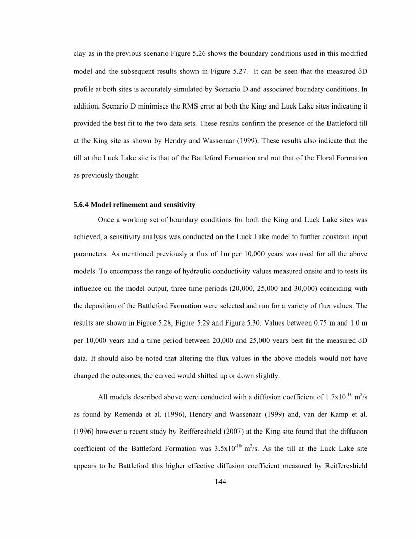
144
clay as in the previous scenario Figure 5.26 shows the boundary conditions used in this modified
model and the subsequent results shown in Figure 5.27. It can be seen that the measured δD
profile at both sites is accurately simulated by Scenario D and associated boundary conditions. In
addition, Scenario D minimises the RMS error at both the King and Luck Lake sites indicating it
provided the best fit to the two data sets. These results confirm the presence of the Battleford till
at the King site as shown by Hendry and Wassenaar (1999). These results also indicate that the
till at the Luck Lake site is that of the Battleford Formation and not that of the Floral Formation
as previously thought.
5.6.4 Model refinement and sensitivity
Once a working set of boundary conditions for both the King and Luck Lake sites was
achieved, a sensitivity analysis was conducted on the Luck Lake model to further constrain input
parameters. As mentioned previously a flux of 1m per 10,000 years was used for all the above
models. To encompass the range of hydraulic conductivity values measured onsite and to tests its
influence on the model output, three time periods (20,000, 25,000 and 30,000) coinciding with
the deposition of the Battleford Formation were selected and run for a variety of flux values. The
results are shown in Figure 5.28, Figure 5.29 and Figure 5.30. Values between 0.75 m and 1.0 m
per 10,000 years and a time period between 20,000 and 25,000 years best fit the measured δD
data. It should also be noted that altering the flux values in the above models would not have
changed the outcomes, the curved would shifted up or down slightly.
All models described above were conducted with a diffusion coefficient of 1.7x10⁻¹⁰ m2/s
as found by Remenda et al. (1996), Hendry and Wassenaar (1999) and, van der Kamp et al.
(1996) however a recent study by Reiffereshield (2007) at the King site found that the diffusion
coefficient of the Battleford Formation was 3.5x10⁻¹⁰ m2/s. As the till at the Luck Lake site
appears to be Battleford this higher effective diffusion coefficient measured by Reiffereshield

145
(2007) can be used. Figure 5.31 shows the results of the model run with the both till and clay
diffusion coefficients increased to 3.5x10⁻¹⁰ m2/s. It can be seen that the till data is matched quite
well, however, the below the till/clay interface fit is a poor fit to the measured δD profile which
would be expected as all previous measurements in the clay yield a smaller diffusion coefficient.
The next step was to use two effective diffusion coefficients, the measured 1.7x10⁻¹⁰ m2/s in the
clay (Remenda et al., 1996; Hendry and Wassenaar, 1999; van der Kamp et al., 1996) and the
newly measured 3.5x10⁻¹⁰ m2/s in the till (Reiffereshield, 2007). The results using two effective
diffusion coefficients, 1.7x10⁻¹⁰ m2/s in the clay and 3.5x10⁻¹⁰ m2/s in the till are shown in Figure
5.32. There is excellent agreement between both profiles, suggesting that the use of two De is
more appropriate for diffusion of deuterium in the till and clay. The final step in the modelling
was to further constrain time estimates within the model for the two best fit flux values. The
results are shown in Figure 5.33 and Figure 5.34. The measured δD data is best fit with ice cover
times ranging from 15,000 to 20,000 years and the onset of precipitation around 7,500 years.
Thus the overall age of the till ranges from 22,500 and 27,500, which supports the till being of the
Battleford Formation and not the Floral Formation as previously thought.
The above analysis did not explicitly consider underpressuring or overpressuring. The
flow conditions in both models during glaciation were held constant. Using a downward gradient
in the models resulted in an acceptable fit between the model and measured data for both sites.
Whether the downward gradient is the result of underpressuring or some other long-term flow
regime is unknown. Regardless, the acceptable fit between the measured and modelled data is
evidence that the main aspects of the physical behaviour have been captured using the boundary
conditions applied in the models.

146
5.7 Discussion and Conclusions
This chapter presents the findings from the re-examination of the till stratigraphy at a
field site in southern Saskatchewan, through the examination of till geochemistry and pore water
chemistry of the both till and underlying Cretaceous deposits. Samples of the till and underlying
Bearpaw Formation were collected in a series of drilling investigations over varying intervals up
to a maximum depth of 90 m below ground surface. Prior to this work, it was believed the till at
site was that of the Floral Formation. The Battleford Formation was originally thought to be less
than 11 m in thickness at the time of the initial till characterization on site, however studies
conducted at the nearby King site found that the Battleford Formation to be 80 m in thickness
thus opening the door for reinterpretation of the till at this site.
Pore water was extracted from both the clay and till samples and analyzed for deuterium,
oxygen-18 and selected anions. The extensive database of stable isotopes to a depth of 90 m is
unique as extraction and analysis of water samples up to this depth is very rare due to the cost and
difficulty in sample collection.
The use of vertical isotope profiles to provide information into the timing of geologic
events has been found to be successful. Modelling of the vertical deuterium profile was
conducted with the intent to constrain depositional times of the till and thus determine the
formation to which it belongs. The depositional age of the till at the Luck Lake site was found to
be in the range from 22,500 and 27,500 years which is reflective of till deposited during the
Battleford Formation. Additionally the oxidized nature of the Battleford Formation at the Luck
Lake site also provides constraints on the time required for fractures and oxidation which was
previously not well understood. Results from the modelling highlight the advantages to be gained
from using multiple sites with differing geometries, in order to test the validity of the boundary
conditions. In addition, the model boundary conditions provide insight into the method of till

147
deposition during glaciation. The depositional mechanism for the till at the Luck Lake site is that
of melt out till, consistent with the results found by other work conducted in the Battleford
Formation (Sauer and Christiansen, 1991; Shaw 1997).

148
5.8 References
American Society for Testing and Materials (ASTM). 2000a. Standard Test Methods for Liquid Limit, Plastic Limit and Plasticity Index of Soils. Annual Book of Standards, Section 4, Soil and Rock (1). Vol 04-08. D 4318-00. ASTM International, West Conshohocken, Pennsylvania. American Society for Testing and Materials (ASTM). 2000b. Standard Practice for Classification of Soils for Engineering Purposes (Unified Soil Classification System). Annual Book of Standards, Section 4, Soil and Rock (1). Vol 04-08. D 2487-00. ASTM International, West Conshohocken, Pennsylvania. American Society for Testing and Materials (ASTM). 2000c. Standard Test Method for Particle-Size Analysis of Soils. Annual Book of Standards, Section 4, Soil and Rock (1). Vol 04-08. D 422-63. ASTM International, West Conshohocken, Pennsylvania. Bekele, E.B., Rostron, B.J., and Person, M.A. 2003. Fluid pressure implications of erosional unloading , basin hydrodynamics and glaciation in the Western Canada, Alberta Basin. Journal of Geochemical Exploration, 78-79, 143-147 Caldwell, W.G.E. 1968. The Late Cretaceous Bearpaw Formation in the South Saskatchewan River valley. Saskatchewan Research Council, Geology Division, Report #5 Cey, B.D., Barbour, S.L., and Hendry, J.M. 2000. Osmotic flow through a Cretaceous clay in southern Saskatchewan, Canada. Canadian Geotechnical Journal, 38, 1025-1033. Christiansen, E.A. 1968. Pleistocene stratigraphy of the Saskatoon area, Saskatchewan, Canada. Canadian Journal of Earth Sciences, 5, 1167-1173. Christiansen, E.A., 1971. Tills in southern Saskatchewan. In:Goldthwaite, R.P., (Ed.), Tills/A Symposium, Ohio State University Press, pp. 167–183. Christiansen, E.A. 1992. Pleistocene stratigraphy of the Saskatoon area, Saskatchewan, Canada: an update. Canadian Journal of Earth Sciences, 29, 1767-1778. Christiansen, E.A. 2005. Personal Communication Christiansen, E.A. 2005. Glacial Geology of Southern Saskatchewan. R.M Hardy Address, Proceedings of the 57th Canadian Geotechnical, GeoSask 2005, Saskatoon, Saskatchewan. Clark, I. & P. Fritz, 1997, Environmental Isotopes in Hydrogeology, Lewis Publishers, CRC Press. Craig, H. 1961 Isotopic variations in meteoric waters. Science, 133: 1702-1703. Darcy, H. 1856. Dètermination des lois d'ècoulement de l'eau à travers le sable. p. 590–594. In Les Fontaines Publiques de la Ville de Dijon. Victor Dalmont, Paris.

149
Desaulniers, D.E., Cherry, J.A., Fritz, P., 1981. Origin, age and movement of pore water in argillaceous quaternary deposits at four sites in southwestern Ontario. Journal of Hydrology 50, 231–257. Drever, J.I. 1982. The geochemistry of natural waters. Prentice Hall, Inc, Englewood Cliffs, N.J. Entwisle D C and Reeder S. 1993. New apparatus for pore fluid extraction from mudrocks for geochemical analysis. In: Manning D A C, Hall P L and Hughes C R (Eds), Geochemistry of Clay-Pore Fluid Interactions, Chapman and Hall, 365-388. Fortin, G., van der Kamp, G., and Cheery, J.A. 1991. Hydrogeology and hydrochemistry of an aquifer-aquitard system within glacial deposits, Saskatchewan, Canada. Journal of Hydrology 126, 265-292. Gimmi, T., Waber, H. N., Gautschi, A., and Rubel, A. (2007), Stable water isotopes in pore water of Jurassic argillaceous rocks as tracers for solute transport over large spatial and temporal scales, Water Resources Research, 43, W04410. Grasby, S.E, and Chen, Z. 2005. Subglacial recharge into the western Canada Sedimentary Basin — impact of Pleistocene glaciation on basin hydrodynamics, Geological Society of America Bulletin, 117, 500–514. Hendry, M.J., 1982. Groundwater recharge through a heavy textured soil. Journal of Hydrology 63, 201–209. Hendry, M.J., Cherry, J.A., Wallick, E.I., 1986. Origin and distribution of sulfate in a fractured till in southern Alberta, Canada. Water Resources Research 22 (1), 46–61. Hendry, M.J., Schwartz, F.W., 1988. An alternative view on the origin of chemical and isotopic patterns in groundwater from the Milk River Aquifer, Canada. Water Resources Research 24, 1747–1763. Hendry, M.J. and Wassenaar, L.I. 1999. Implications of the distribution of δD in pore waters for groundwater flow and the timing of geologic events in a thick aquitard system. Water Resources Research, 35, 1751-17560. Hendry, M.J., L.I. Wassenaar, and T. Kotzer. 2000. Chloride and chlorine isotopes (36^Cl and delta 37^Cl) as tracers of solute migration in a thick, clay-rich aquitard system. Water Resources Research 36, no. 1: 285–296. Hendry, M.J., Kelln, C.J., Wassenaar, L.I., and Shaw, J. 2004.Characterizing the hydrogeology of a complex clay-rich aquitards system using detailed vertical profiles of the stable isotopes of water. Journal of Hydrology, 293, 47-56. Hoefs, J. 2004. Stable Isotope Geochemistry. Springer-Verlag Berlin. 5th Edition. Keller, C.K., van der Kamp, G., and Cherry, J.A. 1986. Fracture permeability and groundwater flow in clayey till near Saskatoon, Saskatchewan. Canadian Geotechnical Journal, 23, 229-240.

150
Keller, K.C., van der Kamp, G., Cherry, J.A., 1988. Hydrogeology of two Saskatchewan Tills. I. Fractures, bulk permeability, and spatial variability of downward flow. Journal of Hydrology 101, 97–121. Kelln, C.J., Wassenaar, L.I., and Hendry, M.J. 2001. Stable isotope (delta 18O, delta D) of porewaters in clay-rich aquitards: A comparison and evaluation of measurement techniques. Ground Water Monitoring and Remediation, 21(2), 108-116. Koehler, G., Wassenaar, L.I., Hendry, M.J., 2000. An automated technique for measuring δD and d18O values of pore water by direct CO2- and H2-equilibration. Analytical Chemistry 72 (21), 5659–5664. Neuzil CE. 1993. Low fluid pressure within the Pierre Shale: a transient response to erosion. Water Resources Research, 29(7), 2007–2020. Neuzil, C. E. 1994. How permeable are clays and shales? Water Resources Research, 30(2), 145–150. Peterson, R. 1958. Rebound in the Bearpaw Shale, Western Canada. GSA Bulletin, 69, 1113-1124. Patterson, R.J., Frape, S.K., Dykes, L.S., and McLeod, R.A. 1978. A coring and squeezing technique for the detailed stuffy of subsurface water chemistry. Canadian Journal of Earth Sciences, 15, 162-169. Remenda, V.H. 1993. Origin and migration of natural groundwater tracers in thick clay tills of Saskatchewan and the Lake Agassiz clay plain. PhD Thesis. University of Waterloo. Remenda, V.H., Cherry, J.A., and Edwards, T.W.D. 1994. Isotopic composition of old ground water from Lake Agassiz: implications for late Pleistocene climate. Science 266, 1975-1978 Remenda, V.H., G. van der Kamp, and J.A. Cherry. 1996. Use of vertical profiles in delta18O to constrain estimates of hydraulic conductivity in a thick, unfractured till. Water Resources Research 32, no. 10: 2979–2987. Reiffereshield, L. 2007. In situ measurement of the coefficient of molecular diffusion in fine grained till. MSc. Thesis, University of Saskatchewan. Ross, W.C. 1986. Atomic absorption method for quantitative determination of carbonates in tills. Saskatchewan Research Council (SRC), Technical Report No. 214. Rowe, K.R. 1987. Pollutant transport through barriers. Geotechnical Practice for Waste Disposal, Special Pub. No. 13, R.C. Woods (ed.), ASCE, New York, N.Y. 159-181. Sacchi, E, Michelot, J.L., Pitsch, H. , Lalieux, P., and Aranyossy, J.F. 2001. Extraction of water and solutes form argillaceous rocks for geochemical characterization: Methods, processes, and current understanding. Journal of Hydrogeology, 9, 17–33

151
Sauer, E.K, Egeland, A.K., and Christiansen, E.A. 1993. Preconsolidation of tills and intertill clays by glacial loading in southern Saskatchewan, Canada. Canadian Journal of Earth Science, 30(3), 420-433. Sauer, E.K. and Christiansen, E.A. 1991. Preconsolidation pressures in the Battleford Formation, southern Saskatchewan, Canada. Canadian Journal of Earth Science, 28, 1616-1623. Sauer, E.K., Gareau, L.F, and Christiansen, E.A. 1990. Softening of overconsolidated Cretaceous clays by glacial erosion. Quarterly Journal of Engineering Geology, 23, 307-324. Schreiner, B.T. 1990. Lithostratigraphic correlation of Saskatchewan tills, a mirror image of Cretaceous bedrock. Ph.D. Thesis, University of Saskatchewan, Saskatoon Scott, J.S., and Brooker, E.W. 1968. Geological and engineering aspects of Upper Cretaceous shales in Western Canada. Geological Survey of Canada Paper, 66-37. Shackelford, C.D., and Daniel, D.E. 1991. Diffusion in saturated soil. I: Background, Journal of Geotechnical Engineering, 117, 485–506. Shaw, J., and Hendry, M.J. 1998. Hydrogeology of a thick clay till and Cretaceous clay sequence, Saskatchewan, Canada. Canadian Geotechnical Journal, 35, 1041-1052. Simpkins, W.W., Bradbury, K.W., 1992. Groundwater flow, velocity, and age in a thick, fine-grained till unit in southeastern Wisconsin. Journal of Hydrology 132, 283–319. van der Kamp, G., and Jaworski, E.J. 1989. Luck Lake irrigation project: groundwater monitoring to December, 1989. Saskatchewan Research Council, Publication No. R-1220-5-C-89. van der Kamp, G., D.R. Van Stempvoort, and L.I. Wassenaar.1996. The radial diffusion method, 1. Using intact cores to determine isotopic composition, chemistry, and effective porosities for groundwater in aquitards. Water Resources Research 32, no. 6: 1815–1822. Van Stempvoort, D. R., Hendry, J.M., Schoenau, J.J., Krouse, H.R. 1994. Sources and dynamics of sulfur in weathered till, Western Glaciated Plains of North America. Chemical Geology, 11, 35-56. Wilson, A. M., Fenstemaker, T., Sharp Jr, J.M. 2003. Abnormally pressured beds as barriers to diffusive solute transport in sedimentary basins. Geofluids, 3, 203-212.

152
Table 5.1 Relative abundance for the stable isotopes of oxygen and hydrogen.
Element Isotope Abundance (%) 1H 99.984 Hydrogen 2H or D 0.015 16O 99.76 17O 0.037 18O 0.204 Oxygen 37Cl 24.47
Table 5.2 Water level readings.
Piezometer ID (Depth to screen, m)
Piezometer location Water level (mbgs)
03-Nov-05
Water level (mbgs)
25-Sept-06 90-01 (45)
51o 04.044' N 107o 02.554' W
6.59 6.41
90-02 (30.5)
51o 04.040' N 107o 02.554' W
3.97 3.77
91-01 (24.0)
51o 04.033' N 107o 02.557' W
2.21 2.24
91-03 (12.8)
51o 04.035' N 107o 02.541' W
2.3 2.36
91-04 (8.1)
51o 04.034' N 107o 02.547' W
2.21 2.06
91-05 (3.0)
51o 04.040' N 107o 02.546' W
2.13 2.26

153
Table 5.3 Till and Bedrock Geochemistry results.
Depth below ground surface (m)
Ca (wt %)* Mg (wt%)* Total Carbonate (mL CO2/g)
Zn (ppm)
3.33 2.31 0.88 21.0 77 6.4 2.53 1.12 24.5 68
9.42 2.34 0.97 22.0 71 12.58 2.79 1.18 26.5 67 15.61 2.79 0.97 24.5 69 18.61 3.63 1.09 30.3 72 21.6 3.69 1.17 31.4 70
24.72 3.02 1.09 26.9 71 27.93 3.24 1.21 29.3 68 29.27 3.69 1.33 32.9 74
30.73 0.61 0.45 7.6 105 32.3 0.69 0.53 8.7 94 35.4 0.70 0.57 9.2 87
38.33 1.43 0.69 14.3 79 41.31 0.68 0.51 8.5 93 45.88 0.37 0.41 5.8 122
* from Remenda (1993). start of bedrock
Table 5.4 Carbonate contents from tills in southern Saskatchewan (modified from
Christiansen, 2005).
Unit Number of
samples analyzed
Mean carbonate content
(mL CO2/g)
Standard deviation (mL CO2/g)
Battleford Formation 552 28.2 13.5 Floral Formation 1855 38.2 13.9 Saskatoon Group 2407 35.9 14.4 Warman Formation 561 16.6 5.0 Dundurn Formation 1048 29.1 8.3 Mennon Formation 310 14.1 4.5 Sutherland Group 1919 23.0 9.7

154
Table 5.5 Zinc values from tills in southern Saskatchewan (modified from Schreiner, 1990).
Unit Number of
samples analyzed
Mean Zinc value (ppm)
Standard deviation
(ppm) Battleford Formation 39 66.9 22.2 Upper Floral Formation 97 60.0 13.1 Lower Floral Formation 103 68.4 15.4 Saskatoon Group 239 64.9 16.3 Warman Formation 120 90.7 30.6 Dundurn Formation 145 84.5 34.3 Mennon Formation 98 93.3 50.5 Sutherland Group 364 88.8 37.8
Table 5.6 Model Boundary Conditions Luck Lake site.
Boundary Conditions Model Stages Scenario A Scenario B Scenario C Scenario D
1. SEEP/W - groundwater seepage
Top of Till: CF (varied) Bottom. of Clay: CH (50 mbgs)
Top of Till: CF (varied) Bottom. of Clay: CH (50 mbgs)
Top of Till: CF (varied) Bottom. of Clay CH (50 mbgs)
Top of Till: CF (varied) Bottom. of Clay: CH (50 mbgs)
2. CTRAN/W - initial concentrations
Till δD: -178‰ Clay δD – 142‰
Till δD – 178‰ Clay δD – 142‰
Till δD – 178‰ Clay δD – 142‰
Till δD – 178‰ Clay δD – 142‰
3. CTRAN/W - glaciation (ice cover)
Top of Till: -178‰ Bottom. of Clay: -142‰
Top of Till: -190 ‰ Bottom. of Clay: -142‰
Top of Ice: -178 ‰ Bottom. of Ice. : -178 ‰ Bottom. of Clay -142‰
Top of Ice: -178‰ Bottom. of Ice. : -178‰ Bottom. of Clay: -142‰
4. CTRAN/W - post glaciation (modern precipitation)
Top of Till: -136‰ Bottom. of Clay: -142‰
Top of Till: -136‰ Bottom. of Clay: -142‰
Top of Till: -136‰ Bottom. of Clay: -142‰
Top of Till: -136‰ Bottom. of Clay: -142‰
CF – constant flux boundary, CH – constant head boundary

155
Table 5.7 Model Boundary Conditions King site.
Boundary Conditions Model Stages Scenario A Scenario B Scenario C Scenario D
1. SEEP/W - groundwater seepage
Top of Till: CF (varied) Bottom. of Clay: CH (50 mbgs)
Top of Till: CF (varied) Bottom. of Clay: CH (50 mbgs)
Top of Till: CF (varied) Bottom. of Clay: CH (50 mbgs)
Top of Till: CF (varied) Bottom. of Clay: CH (50 mbgs)
2. CTRAN/W - initial concentrations
Till: -178‰ Clay: -144‰
Till: -178‰ Clay: -144‰
Till: -178‰ Clay: -144‰
Till: -178‰ Clay: -144‰
3. CTRAN/W - glaciation (ice cover)
Top of Till: -178‰ Bottom. of Clay: -142‰
Top of Till: -190‰ Bottom. of Clay: -142‰
Top of Ice: -178 ‰ Bottom. of Ice. : -178 ‰ Bottom. of Clay: -142‰
Top of Ice: -178 ‰ Bottom. of Ice. : -178 ‰ (till below ice) Bottom. of Clay: -142‰
4. CTRAN/W - post Glaciation (modern precipitation)
Top of Till: -136‰ Bottom. of Clay: -144‰
Top of Till: -136‰ Bottom. of Clay: -144‰
Top of Till: -136‰ Bottom. of Clay: -144‰
Top of Till: -136‰ Bottom. of Clay: -144‰
CF – constant flux boundary, CH – constant head boundary
Figure 5.1 Range of specific discharge over which diffusion or mechanical dispersion
controls hydrodynamic diffusion (modified from Rowe, 1987).

156
Figure 5.2 Global meteoric water line (modified from Craig, 1961).
Figure 5.3 Deviations from the meteoric water line resulting from potential fractionation
mechanisms (Clark and Fritz, 1997).

157
TIME Stratigraphic units
Holocene Pike Lake Formation SAND
Haultain Formation SAND & SILT Late
Wisconsin Battleford Formation TILL
TILL Early
Wisconsin
Upp
er T
ill
Uni
t
CLAY/SAND + GRVEL
Sangamon Riddell Member SAND
TILL
CLAY/SAND
Late
Ple
isto
cene
Illionian Sa
skat
oon
Gro
up
Flor
al F
orm
atio
n
Low
er T
ill u
nit
TILL
Warman Formation TILL
Dundurn Formation TILL
Suth
erla
nd G
roup
Mennon Formation TILL
Qua
tern
ary
Early
& M
iddl
e. P
leis
toce
ne
Pre-Illionian
Tertiary Pliocene
Empress
Group SAND & GRAVEL
Bearpaw Formation SILT & CLAY
Judith river Formation SAND & SILT
Cre
tace
ous
Late Cretaceous
Mon
tana
Gro
up
Lea Park Formation SILT & CLAY
Figure 5.4 Stratigraphy of southern Saskatchewan.

158
Figure 5.5 Location of field site in southern Saskatchewan.

159
Figure 5.6 Stratigraphic borehole log and location of samples used. Diamonds were sampled
from Nov 2005, Squares were sampled Sept 2006 and the circles are dried samples used as
part of this investigation from Remenda (1993). Shaded diamonds and squares represent
Shelby tube samples.
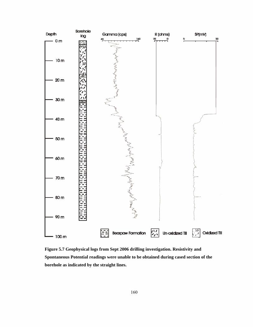
160
Figure 5.7 Geophysical logs from Sept 2006 drilling investigation. Resistivity and
Spontaneous Potential readings were unable to be obtained during cased section of the
borehole as indicated by the straight lines.

161
Figure 5.8 Squeezing apparatus used for pore water extraction consisting of Enerpac hand
jack, hydraulic cylinder and pressure gauge.
Figure 5.9 Complete pore water extraction apparatus.
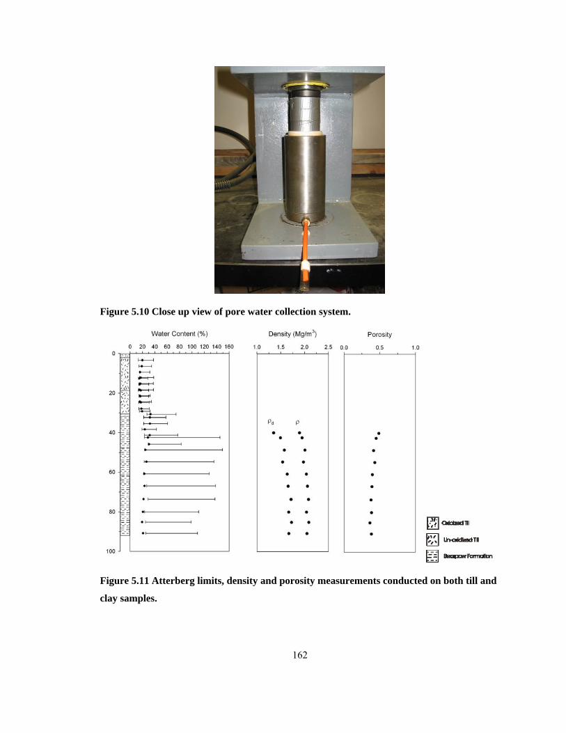
162
Figure 5.10 Close up view of pore water collection system.
Figure 5.11 Atterberg limits, density and porosity measurements conducted on both till and
clay samples.

163
Figure 5.12 Plasticity chart.
10-14
10-13
10-12
10-11
10-100.1
0.2
0.3
0.4
0.5
0.6
0.7
0.8
0.9
1
1.1
Hydraulic conductivity, K (m/s)
Voi
d ra
tio, e
y=0.0918Ln(x)+3.1368→
dia=16.9 mmdia=25.0 mmdia=35.6 mmdia=63.5 mm
Figure 5.13 Hydraulic conductivity versus void ratio, calculated from oedometer tests on the
Bearpaw Formation.

164
Figure 5.14 Till geochemistry – total carbonate and zinc within the till and the upper part of
the clay.
Figure 5.15 Stable Isotope Geochemistry - δD and δ18O profiles with depth.

165
Figure 5.16 Stable isotopes results and the local meteoric water line for Saskatoon. Local
meteoric water line as given by Hendry and Wassenaar (1999).
Figure 5.17 Anion analysis (Cl- and SO4-) for extracted pore water within the till and
underlying clay.

166
Figure 5.18 SRC borehole log.

167
Figure 5.19 Model Scenario A, basal till deposition.

168
(a)
(b)
Figure 5.20 Results for the King site, model scenario A. (a) results from ice cover stage of
the model only (b) final model results, including both ice cover and precipitation.

169
(a)
(b)
Figure 5.21 Results for the Luck Lake site, model scenario A. (a) results from ice cover
stage of the model only (b) final model results, including both ice cover and precipitation.

170
Figure 5.22 Model scenario B, basal till deposition, initial δD values in the till -190.

171
(a)
(b)
Figure 5.23 Results from model scenario B (a) king site (b) Luck Lake site.

172
Figure 5.24 Model scenario C, melt out till deposition, ice located directly on till during
glaciation.
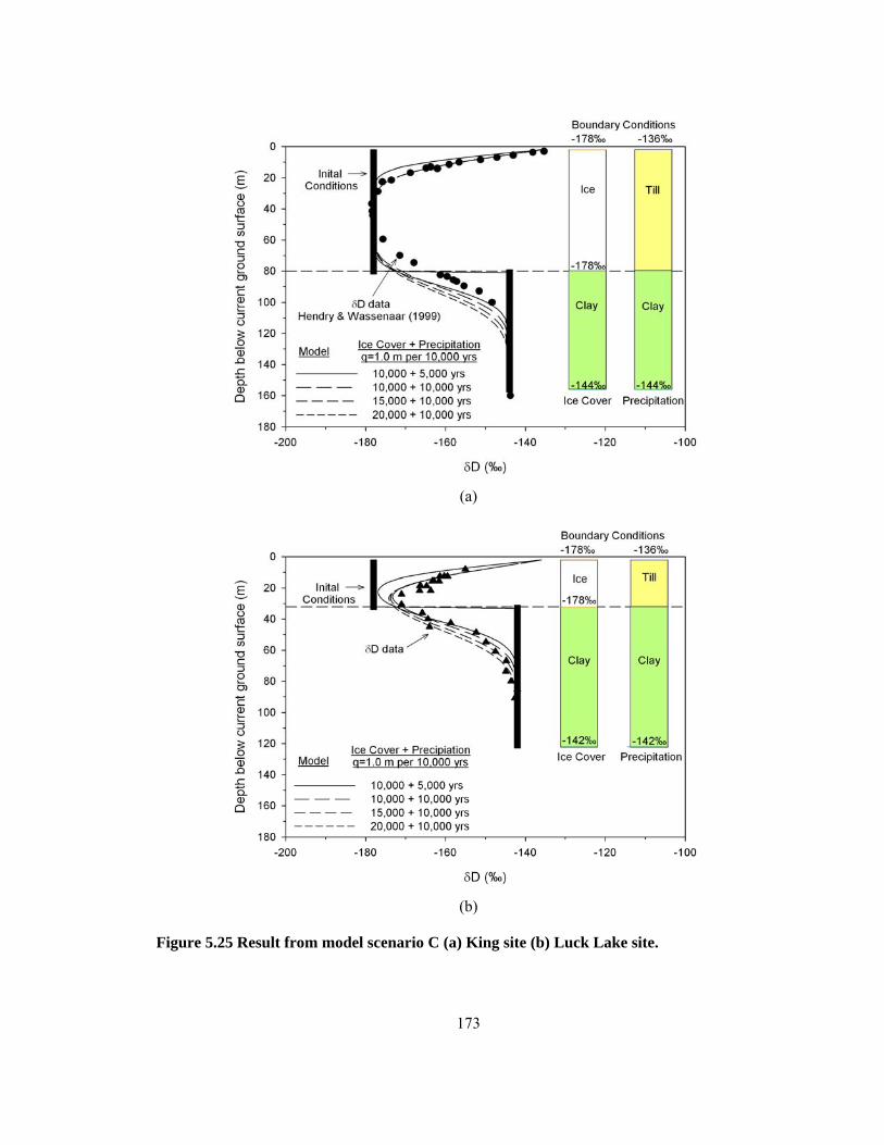
173
(a)
(b)
Figure 5.25 Result from model scenario C (a) King site (b) Luck Lake site.

174
Figure 5.26 Model scenario D, melt out till deposition at Luck Lake site, combination of
ablation and basal melt out till at the King site.

175
(a)
(b)
Figure 5.27 Result from model scenario D (a) King site (b) Luck Lake site.

176
Figure 5.28 Model results for 20,000 years (10,000 ice cover + 10,000 precipitation) over a
variety of constant fluxes.
Figure 5.29 Model results for 25,000 years (15,000 ice cover + 10,000 precipitation) over a
variety of constant fluxes.

177
Figure 5.30 Model results for 30,000 years (20,000 ice cover + 10,000 precipitation) over a
variety of constant fluxes.
Figure 5.31 Model results with the effective diffusion coefficient equal to 3.5x10⁻¹⁰ m2/s in
both the till and clay for 20,000 years over a variety of fluxes.
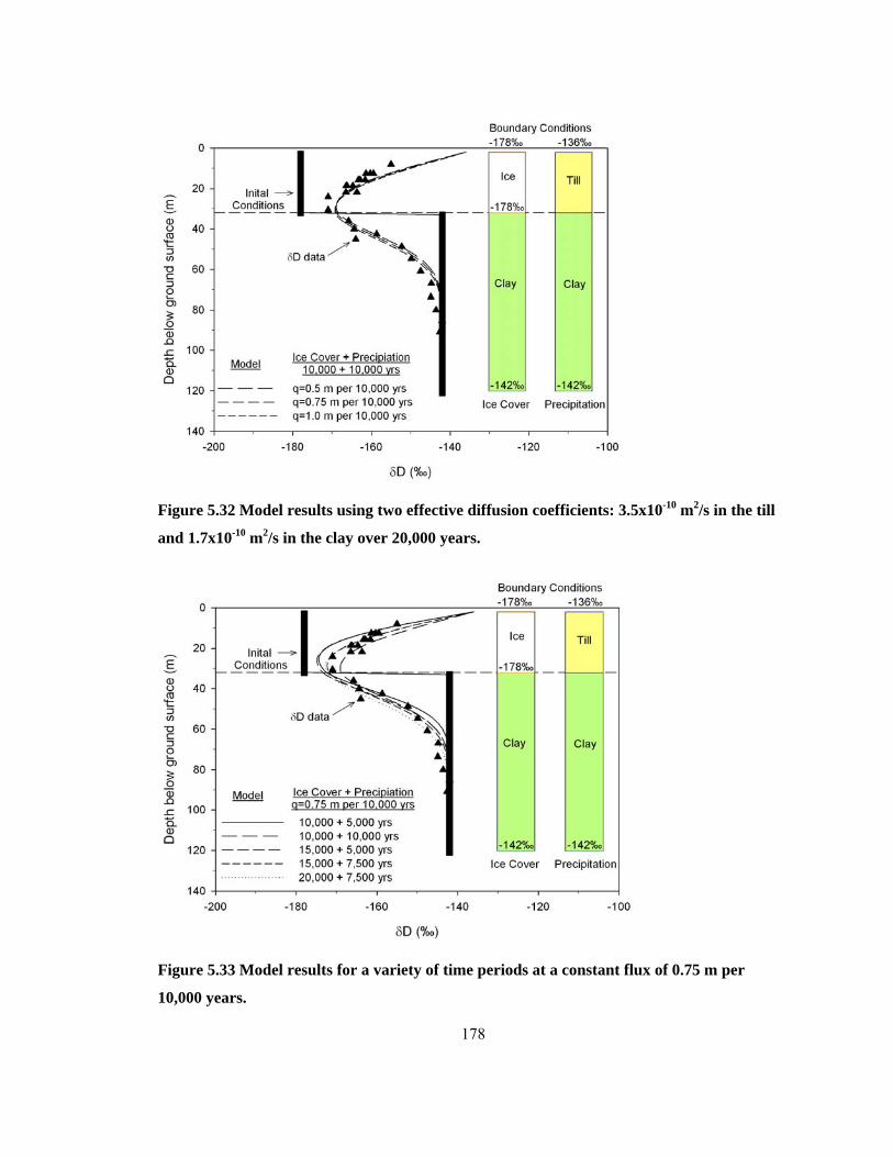
178
Figure 5.32 Model results using two effective diffusion coefficients: 3.5x10⁻¹⁰ m2/s in the till
and 1.7x10⁻¹⁰ m2/s in the clay over 20,000 years.
Figure 5.33 Model results for a variety of time periods at a constant flux of 0.75 m per
10,000 years.

179
Figure 5.34 Model results for a variety of time periods at a constant flux of 1.0 m per 10,000
years.

180
Chapter 6
Conclusions and Recommendations
6.1 General
The objective of this work was to take a multidisciplinary approach to comprehensively
investigate the material properties, mechanical properties and pore water chemistry of a stiff soil,
to determine how these properties relate to the strength of this material, and challenge our ideas
of the hydrogeology and the geological history of the region. This was carried out by (1)
performing a detailed investigation of the material properties and characterization of the
compression behaviour of Bearpaw shale; (2) Examining the time dependent behaviour of a stiff
soil and the transferability of time rate models developed in soft soils to stiff soils; (3) Examining
the swelling potential and behaviour of the Bearpaw and determine the influence of boundary
conditions on this behaviour and (4) constraining the depositional age of materials overlying the
Bearpaw shale. The specific conclusions resulting from the accomplishment of these objectives
are given below.
6.2 Conclusions
This study begins to fill current gaps in the literature on the behaviour of stiff soils. While the
material selected for this research was the Bearpaw shale, it is a material not dissimilar to the
many marine deposits found within the Western Canadian Sedimentary Basin and around the
world and thus the knowledge gained here is transferrable to a number of applications worldwide.
The contributions made were maximized by the multidisciplinary nature of this work which
highlights the strength of taking such approach. The main conclusions of this research are as
follows:

181
• Reduced specimen sizes of 25.0 mm and 16.9 mm in diameter, taken from an initial core
diameter of 76 mm, were found to minimize the effect of disturbance and produce more
reliable results in a stiff clay soil. Due to the brittle nature of this material, a minimum
aspect ratio of 2.5 the oedometer specimens was utilized resulting in a less fractured and
thus less disturbed specimen.
• Through detailed characterization of the Bearpaw shale the apparent depth of softening
was identified to be approximately 67 m based on the measured preconsolidation profile.
The Bearpaw Shale was characterized as to its deformation properties. Parameters Cc and
σp’ were highly sensitive to sample disturbance; however, other parameters such as cv and
k were less dramatically affected by disturbance.
• The isotache theory was found to effectively describe the time-dependent behaviour of
Bearpaw Shale. A constant Cαe/Cc* ratio was observed in loading and unloading.
Therefore, an approximately 10% change in preconsolidation pressure for an increase of
one log cycle of strain rate was measured. Due to the high preconsolidation pressure of
the Bearpaw shale, this 10% corresponds to approximately 1000 kPa. Since creep occurs
in-situ as well as during laboratory testing use of a single parameter such as
preconsolidation pressure to predict geological history in stiff clays is questionable.
• A Swell Equilibrium Limit (SEL) was defined for Bearpaw shale. The SEL was found to
be dependent on initial void ratio or the depth the sample was extracted from. One
dimensional swell pressure measurements reflected the effect of disturbance that was
observed in the stress-strain data. Significant variation in the observed swell pressures
with samples of the same size and depth were found highlighting the importance of multi-
sample testing. Finally, the specialized triaxial swell tests enable the determination of

182
both heave and swelling induced stress behaviour in comparison to the traditional one
dimensional swell test.
• The depositional age of the till overlying the Bearpaw shale ranged from 22,500 and
27,500 years indicating the entire till thickness is that of the Battleford Formation,
contrary to what was originally thought. The advantages to be gained from using multiple
sites with differing geometries, in order to test the validity of the analysis were also
highlighted.
The multidisciplinary approach used in this study allows application of the results across
many areas of research. For example, creep processes are typically not accounted for or well
understood when assessing geological history of a material however the parameters that are often
used in this capacity (i.e. preconsolidation pressure) are influenced by creep processes. The
fundamental potential implications that result from misinterpretation of data resulting from the
link between these areas of study show the importance a multidisciplinary study and benefits that
can be gained from taking such an approach.
6.3 Recommendations
Recommendations based on the observations, experience and the results of this
investigation are as follows.
• Sample disturbance was observed to have significant effects on the behaviour of Bearpaw
shale. Further investigation in to the disturbance of stiff soils could lead to the
development of more detailed and specific disturbance criteria for these materials and
non-destructive methods of assessing sample quality. For example, radiographic methods
could be employed looking for the presence of fractures in test specimens. The suction in
the specimen could also be an indicator of sample disturbance or potential variability in
183
oedometric swell pressure measurements. Unfortunately, the suctions in the samples here
exceeded the 1500 kPa limit for axis translation or high capacity tensiometric
measurement methods and as such were deemed to be outside the scope of the present
study.
• The Bearpaw shale was observed to experience time dependent behaviour that can be
described in a similar framework to much softer clays. This study also indicated a well-
defined link between rebound and creep. This very interesting finding warrants additional
research.
• The combination of parallel streams of research focused on the characterisation of the
compressibility of a geological deposit combined with a numerical model of its
hydrogeological history has been used to constrain the time frame of recent geological
events. If this strategy were to be applied to softer sediments, the coupled interaction
between these two processes could be investigated in greater detail.

Appendix A
A.1 Water Content

185
A.2 Volume Measurements

186
A.3 Atterberg Limits

187

188

189

190

191

192

193

194

195

196

197

198

199

200
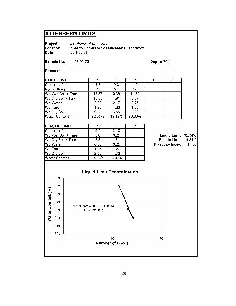
201

202
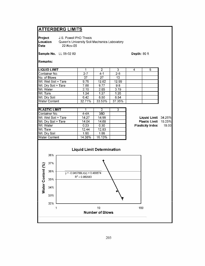
203

204
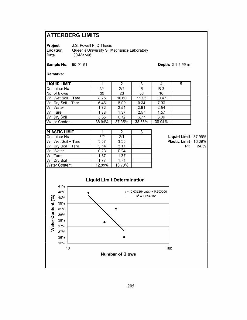
205

206

207

208

209
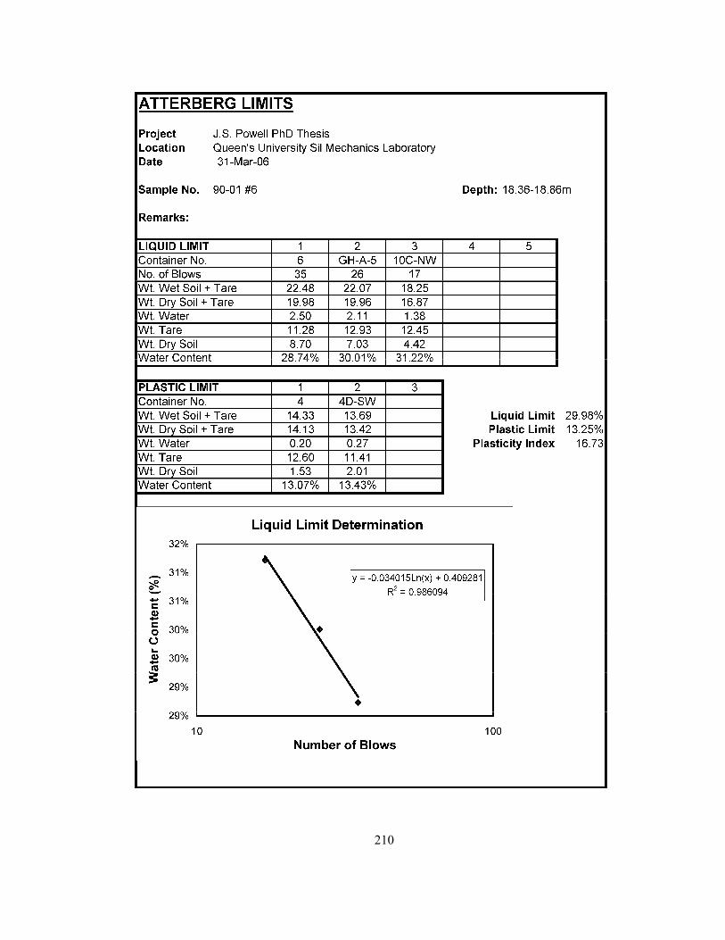
210

211

212

213

214

215
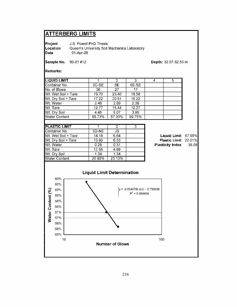
216

217

218

219

220

221
A.4 Grain Size Analysis

222

223

224

225

226
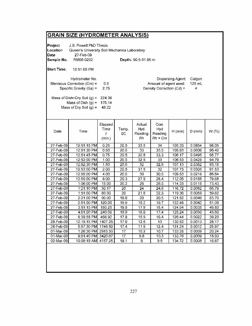
227

228
Appendix B
B.1Oedometer Apparatus
The one dimensional consolidation tests were conducted in an oedometer apparatus and
displacement measurements were taken with a Wykeham Ferrance 0.002 mm accuracy dial
gauge. Tests were conducted in accordance with D4546-96 using the Constant Volume approach
for determining swell pressure. To reduce the amount of evaporation during the length of the test,
plastic was used to cover the water bath. Photographs of apparatus set up can be found in Figure
B.1. Slight modification to the oedometer apparatus was also conducted in order to achieve large
stresses during the tests. The hanger rod was lengthened to accommodate more weight (a
maximum of 200kg) during the tests and thus achieve very high loads. As discussed in Chapter 2,
a variety of sample sizes were tested in the oedometer that ranged in size from 63.5 mm to 16.9
mm. To accommodate such small sizes, new soil cutters and collars were developed to fit within
the existing oedometer bases. Details specifications of these cutters are shown in Figure B.2,
Figure B.3 and Figure B.4.
(a)
Dial gauge
Plastic to minimize evaporation

229
(b) (c)
Figure B.1 Photographs of oedometer apparatus
Extended hanger rod
200 kg of weight

230
Figure B.2 Specifications for 35.6 mm diameter cutter and collar assembly.

231
Figure B.3 Drawings for 25.0 mm diameter cutter and collar assembly.

232
Figure B.4 Drawings for 16.9 mm diameter cutter and collar assembly.

233
B.2Constant Rate of Strain (CRS) Apparatus
The CRS apparatus was designed to accommodate the 16.9 mm diameter specimens. The
steel base was designed with two drainage pathways that originated from the bottom porous stone
and were connected to external burettes enabling the system to be flushed prior to testing. A
GP50 pressure transducer was used to monitor pore pressures during testing. The 16.9 mm cutter,
collar and top cap from earlier odometer testing were used inside the base to house the sample.
The base was designed to accommodate a series of diameter samples with in use of a steel insert
designed for the specified cutter diameter. The base contained dual drainage the system to be
flushed. A LVDT was used to measure vertical displacements. Load was applied to the sample
via the Wykeham Ferrance load frame. The sensors were monitored using a HBM GC data
acquisition system. Photographs of the CRS set up are presented in Figure B.5.
(a) (b)
Figure B.5 Photographs of CRS apparatus.
Load cell
LVDT
Pressure Transducer

234
B.3CRS Testing Procedure
• Prepare specimen in cutting ring and record the weight of both the specimen and the
cutter and the height of the specimen. Cuttings from specimen preparation were used to
determine the initial water content of specimen.
• Clean out remaining any water from the cell. Flush lines with de-aired water to remove
air bubbles. Put in bottom ceramic stone, flush with water thoroughly. Remove excess
water with a paper towel.
• Place a little bit of vacuum grease on the base of the cutter to ensure a good seal.
• Place cutter in the collar and add top porous stone to the top of the specimen.
• Start the data acquisition system.
• Place collar assembly along with top cap into the cell. Tighten nuts, in a clockwise
manner, to the fix the collar down to the base. At the same time raise the base so that
the loading cap is almost touching the load cell.
• Once finished tightening the nuts, turn on the loading frame to bring the top cap in
contact with the load cell. Once contact is made, turn off the machine.
• Fill the cell with de-aired water and open the lines to the burettes. Monitor specimen as
swell pressure develops.
• Once load equilibrates (swell pressure reached) adjust loading frame to speed desired.
Close burette lines and start the loading frame to begin compressing specimen under
constant strain rate.
• Upon completion of the test, dismantle the apparatus, take post test measurements of
sample and determine water content of removed sample.
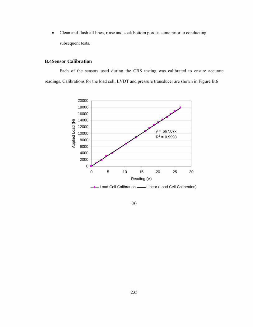
235
• Clean and flush all lines, rinse and soak bottom porous stone prior to conducting
subsequent tests.
B.4Sensor Calibration
Each of the sensors used during the CRS testing was calibrated to ensure accurate
readings. Calibrations for the load cell, LVDT and pressure transducer are shown in Figure B.6
y = 667.07xR2 = 0.9998
0
2000
40006000
8000
10000
12000
1400016000
18000
20000
0 5 10 15 20 25 30
Reading (V)
App
lied
Load
(N)
Load Cell Calibration Linear (Load Cell Calibration)
(a)

236
y = 0.0272x + 0.2433R2 = 1
0
0.05
0.1
0.15
0.2
0.25
0.3
0.35
0.4
0.45
-10 -5 0 5 10
Reading (V)
Dis
plac
emen
t (in
)
LVDT Calibration Linear (LVDT Calibration)
(b)
y = 684.84x - 3.2944R2 = 1
y = 684.02x - 2.9121R2 = 1
0
100200
300
400500
600
700800
900
0 0.2 0.4 0.6 0.8 1 1.2 1.4
Reading (V)
Appl
ied
Pres
sure
(kPa
)
Calibration 1 Calibration 2Linear (Calibration 1) Linear (Calibration 2)
(c)
Figure B.6 Sensor Calibration (a) Load Cell (b) LVDT (c) Pressure transducer.

237
B.5Apparatus Compliance
B.5.1Oedometer Compliance
Steel specimens, with similar dimension to the actual soil specimens tested were placed
in the oedometer cells and loaded incrementally until the maximum load of 200 kg was applied,
followed by unloading. The results from a typical compliance test and its duplicate are shown in
Figure B.7. For each oedometer tests the same set of porous stones corresponding to the soil tests
were used in the compliance testing. Hysteresis is seen between the initial loading and unloading.
To ensure consistency and repeatability, each compliance test was duplicated. This was done by
completely disassembling the apparatus then reassembling and performing additional compliance
tests.
Vertical effective stress, σv' (kPa)
102 103 104 105 106
Cha
nge
in R
eadi
ng (m
m)
-0.5
-0.4
-0.3
-0.2
-0.1
0.0
Apparatus CompressibiltyDuplicate
Figure B.7 Oedometer compliance test results
Prior to the analysis of the oedometer data, the results were corrected for machine
compressibility. . Figure B.8 compares the use of applying a compliance correction using only the

238
loading curve and then using both the unloading and loading curves. The difference between
using both the unloading and loading curves in comparison to just using the loading was
negligible under the stress interval tested as the slopes of the normal compression line (Cc) and
the rebound line (Cs) were unchanged between the two curves. Therefore, only the loading curve
was used to correct the data. To apply the correction, a function was assigned to the appropriate
loading curve which was then used to adjust the oedometer readings to account for the machine
compressibility that would be present over that particular stress interval. The compliance
correction shifts the stress-strain curve upward. The correction is less in the low stress portion of
the curve however becomes more significant in the higher stress portion of the curve. This shift in
the curve results in a larger preconsolidation pressure as well as lower values for the normal
compression line (Cc) and the rebound line (Cs) and therefore failing to correct for machine
compressibility would give you an underestimate of these parameters.
Vertical effective stress, σv' (kPa)
101 102 103 104 105 106
Sam
ple
heig
ht (m
m)
4.5
5.0
5.5
6.0
6.5
7.0
7.5
UncorrectedCorrected loading curveCorrected loading & unloading curve
Figure B.8 Example of adjustment to raw readings when corrected for compliance

239
B.5.2CRS Compliance
Compressibility of the CRS apparatus was also measured and accounted for in the testing
program. A steel sample was built into the apparatus and loaded to a maximum load of 15000 N.
The compliance testing was conducted using the same set up as the regular tests. The frame speed
used was 0.008 mm/min corresponding to the middle speed used in the testing program.
Subsequent compliance testing at various speeds was conducted to ensure the machine
compressibility was not rate dependent. Figure B.9 shows the machine compressibility used to
correct the CRS data. As with the oedometer tests, to apply the correction a function was assigned
to the compliance curve which was then used to adjust the LVDT readings to account for the
machine compressibility that would be present over that particular stress interval.
y = 1.333E-16x3 - 4.810E-11x2 + 7.843E-06x - 8.344E-03R2 = 9.990E-01
0
0.05
0.1
0.15
0.2
0.25
0.3
0.35
0.4
0.45
0.5
2400 22400 42400 62400 82400 102400 122400
Pressure (kPa)
Dis
plac
emen
t (m
m)
0.0008A Trendline_test Poly. (0.0008A)
Figure B.9 CRS compliance data.

240
B.6Oedometer Test Results
An example of typical oedometer test results are presented below that display the data
analysis that was conducted on all oedometer test data presented in Chapter 2 and 3. Figure B.10
presents the loading results including the determination of end of primary consolidation for a
typical test. Figure B.11 presents the unloading increment plots. Figure B.12 shows a typical
summary plot for the same test, using the end of primary consolidation points determined in
Figure B.10. Calculation of Cc and Cs are shown in Figure B.13 followed by the preconsolidation
or yield stress determination in Figure B.14.
10-5
100
105-0.08
-0.06
-0.04
-0.022345
678910111213141516171819
20
(a)
Unc
orre
cted
δ h
eigh
t (m
m)
Time (min)-0.5 0 0.5 1
-0.05
-0.04
-0.03
-0.02y=-0.0187x-0.0264 (r2=0.9993
(b)
log(time in min)
Cor
rect
ed δ
hei
ght (
mm
)
10-5
100
105-0.06
-0.04
-0.02
0
-0.044615→
(c)
Cor
rect
ed δ
hei
ght (
mm
)
Time (min)2 2.5 3 3.5
-0.06
-0.055
-0.05
-0.045
y=-0.0060x-0.0387 (r2=0.9921)
(d)
Cor
rect
ed δ
hei
ght (
mm
)
log(time in min)
(a) Load 1

241
10-5
100
105-0.2
-0.15
-0.1
-0.05
0
234567891011121314151617
(a)
Unc
orre
cted
δ h
eigh
t (m
m)
Time (min)0.2 0.4 0.6 0.8 1
-0.12
-0.11
-0.1
-0.09
y=-0.0325x-0.0891 (r2=0.9995)
(b)
log(time in min)
Cor
rect
ed δ
hei
ght (
mm
)10
-510
010
5-0.16
-0.14
-0.12
-0.1
-0.08
-0.12621→
(c)
Cor
rect
ed δ
hei
ght (
mm
)
Time (min)2 2.5 3 3.5
-0.15
-0.145
-0.14
-0.135y=-0.0108x-0.1138 (r2=0.9949)
(d)
Cor
rect
ed δ
hei
ght (
mm
)log(time in min)
(b) Load 2
10-5
100
105-0.4
-0.35
-0.3
-0.25
-0.2 234567891011121314151617181920
(a)
Unc
orre
cted
δ h
eigh
t (m
m)
Time (min)0 0.5 1 1.5
-0.3
-0.25
-0.2y=-0.0615x-0.1980 (r2=0.9979)
(b)
log(time in min)
Cor
rect
ed δ
hei
ght (
mm
)
10-5
100
105-0.35
-0.3
-0.25
-0.2
-0.15
-0.28233→
(c)
Cor
rect
ed δ
hei
ght (
mm
)
Time (min)1 2 3 4
-0.34
-0.32
-0.3
-0.28y=-0.0185x-0.2570 (r2=0.9950)
(d)
Cor
rect
ed δ
hei
ght (
mm
)
log(time in min)
(c) Load 3

242
10-5
100
105-0.7
-0.6
-0.5
-0.4
-0.3
23456789101112131415161718192021
(a)
Unc
orre
cted
δ h
eigh
t (m
m)
Time (min)0 0.5 1 1.5
-0.55
-0.5
-0.45
-0.4
-0.35
y=-0.1120x-0.3779 (r2=0.9987)
(b)
log(time in min)
Cor
rect
ed δ
hei
ght (
mm
)10
-510
010
5-0.7
-0.6
-0.5
-0.4
-0.3
-0.53798→
(c)
Cor
rect
ed δ
hei
ght (
mm
)
Time (min)1.5 2 2.5 3 3.5
-0.62
-0.6
-0.58
-0.56
-0.54y=-0.0398x-0.4811 (r2=0.9969)
(d)
Cor
rect
ed δ
hei
ght (
mm
)log(time in min)
(d) Load 4
10-5
100
105-1.4
-1.2
-1
-0.8
-0.62345678
91011121314151617181920
(a)
Unc
orre
cted
δ h
eigh
t (m
m)
Time (min)0.5 1 1.5
-1
-0.95
-0.9
-0.85
-0.8y=-0.2024x-0.6844 (r2=0.9978)
(b)
log(time in min)
Cor
rect
ed δ
hei
ght (
mm
)
10-5
100
105-1.4
-1.2
-1
-0.8
-0.6
-1.0202→
(c)
Cor
rect
ed δ
hei
ght (
mm
)
Time (min)2 2.5 3 3.5
-1.15
-1.1
-1.05
-1
-0.95
y=-0.0453x-0.9451 (r2=0.9959)
(d)
Cor
rect
ed δ
hei
ght (
mm
)
log(time in min)
(e) Load5

243
10-5
100
105-1.8
-1.6
-1.4
-1.2
-1
23456789101112131415161718
(a)
Unc
orre
cted
δ h
eigh
t (m
m)
Time (min)0.5 1 1.5
-1.5
-1.4
-1.3
-1.2
y=-0.1884x-1.1529 (r2=0.9999)
(b)
log(time in min)
Cor
rect
ed δ
hei
ght (
mm
)10
-510
010
5-1.6
-1.4
-1.2
-1
-0.8
-1.468→
(c)
Cor
rect
ed δ
hei
ght (
mm
)
Time (min)2 2.5 3 3.5
-1.54
-1.52
-1.5
-1.48
-1.46
y=-0.0389x-1.4030 (r2=0.9971)
(d)
Cor
rect
ed δ
hei
ght (
mm
)log(time in min)
(f) Load 6
10-5
100
105-2.1
-2
-1.9
-1.8
-1.723456
789101112131415161718
(a)
Unc
orre
cted
δ h
eigh
t (m
m)
Time (min)0.5 1 1.5
-1.8
-1.75
-1.7
-1.65
-1.6
y=-0.1477x-1.5676 (r2=0.9991)
(b)
log(time in min)
Cor
rect
ed δ
hei
ght (
mm
)
10-5
100
105-2
-1.8
-1.6
-1.4
-1.8206→
(c)
Cor
rect
ed δ
hei
ght (
mm
)
Time (min)2 2.5 3 3.5
-1.88
-1.86
-1.84
-1.82
y=-0.0271x-1.7741 (r2=0.9985)
(d)
Cor
rect
ed δ
hei
ght (
mm
)
log(time in min)
(g) Load 7

244
10-5
100
105-2.6
-2.5
-2.4
-2.3
-2.2 2345678910111213141516 171819202122232425262728293031323334
(a)
Unc
orre
cted
δ h
eigh
t (m
m)
Time (min)0.5 1 1.5
-2.1
-2.05
-2
-1.95y=-0.1225x-1.8959 (r2=0.9993)
(b)
log(time in min)
Cor
rect
ed δ
hei
ght (
mm
)10
-510
010
5-2.2
-2.1
-2
-1.9
-1.8
-2.1006→
(c)
Cor
rect
ed δ
hei
ght (
mm
)
Time (min)2 3 4 5
-2.2
-2.15
-2.1
-2.05
y=-0.0201x-2.0671 (r2=0.9920)
(d)
Cor
rect
ed δ
hei
ght (
mm
)log(time in min)
(h) Load 8
Figure B.10 Load increments and determination of end of primary consolidation. (a)
uncorrected change in height, (b) corrected change in height accounting for oedometer
compressibility displaying end of primary consolidation, (c) fitted line for log-linear portion
before end of primary consolidation is complete, (d) fitted line for log-linear portion after
end of primary consolidation.

245
10-5
100
105-2.4
-2.38
-2.36
-2.34
234567
891011121314151617
(a)
Unc
orre
cted
δ h
eigh
t (m
m)
Time (min)0.5 1 1.5
-2.18
-2.175
-2.17
-2.165
-2.16
y=0.0115x-2.1809 (r2=0.9834)
(b)
log(time in min)
Cor
rect
ed δ
hei
ght (
mm
)10
-510
010
5-2.2
-2.18
-2.16
-2.14
-2.16→
(c)
Cor
rect
ed δ
hei
ght (
mm
)
Time (min)2 2.5 3
-2.1592
-2.159
-2.1588
-2.1586
-2.1584
y=0.0019x-2.1634 (r2=0.999
(d)
Cor
rect
ed δ
hei
ght (
mm
)log(time in min)
(a) Unload 1
10-5
100
105-2.3
-2.25
-2.2
234567
8910111213141516
(a)
Unc
orre
cted
δ h
eigh
t (m
m)
Time (min)0.5 1 1.5 2
-2.14
-2.12
-2.1
-2.08
y=0.0245x-2.1379 (r2=0.9983)
(b)
log(time in min)
Cor
rect
ed δ
hei
ght (
mm
)
10-5
100
105
-2.14
-2.12
-2.1
-2.08
-2.06
-2.0918→
(c)
Cor
rect
ed δ
hei
ght (
mm
)
Time (min)2 2.5 3 3.5
-2.085
-2.08
-2.075
-2.07
y=0.0093x-2.1094 (r2=0.9993)
(d)
Cor
rect
ed δ
hei
ght (
mm
)
log(time in min)
(b) Unload 2

246
10-5
100
105-2.2
-2.15
-2.1
-2.05
23456789101112131415161718
(a)
Unc
orre
cted
δ h
eigh
t (m
m)
Time (min)0.5 1 1.5 2
-2.04
-2.02
-2
-1.98
y=0.0392x-2.0714 (r2=0.9974)
(b)
log(time in min)
Cor
rect
ed δ
hei
ght (
mm
)10
-510
010
5-2.1
-2.05
-2
-1.95
-1.9938→
(c)
Cor
rect
ed δ
hei
ght (
mm
)
Time (min)2 2.5 3 3.5
-2
-1.99
-1.98
-1.97
y=0.0138x-2.0211 (r2=0.9969)
(d)
Cor
rect
ed δ
hei
ght (
mm
)log(time in min)
(c) Unload 3
10-5
100
105-2.05
-2
-1.95
-1.9
234567
89101112
1314151617(a)
Unc
orre
cted
δ h
eigh
t (m
m)
Time (min)1 1.2 1.4 1.6 1.8
-1.94
-1.92
-1.9
-1.88
y=0.0557x-1.9957 (r2=0.9975
(b)
log(time in min)
Cor
rect
ed δ
hei
ght (
mm
)
10-5
100
105-2
-1.95
-1.9
-1.85-1.8746→
(c)
Cor
rect
ed δ
hei
ght (
mm
)
Time (min)2.6 2.8 3 3.2
-1.87
-1.865
-1.86
-1.855
y=0.0179x-1.9135 (r2=0.9923)
(d)
Cor
rect
ed δ
hei
ght (
mm
)
log(time in min)
(d) Unload 4

247
10-5
100
105-1.9
-1.85
-1.8
-1.75
-1.7
23456789
101112131415161718
(a)
Unc
orre
cted
δ h
eigh
t (m
m)
Time (min)1.4 1.6 1.8 2 2.2
-1.82
-1.8
-1.78
-1.76
-1.74
y=0.0599x-1.8898 (r2=0.9999)
(b)
log(time in min)
Cor
rect
ed δ
hei
ght (
mm
)10
-510
010
5-1.85
-1.8
-1.75
-1.7
-1.7583→
(c)
Cor
rect
ed δ
hei
ght (
mm
)
Time (min)2 2.5 3 3.5
-1.76
-1.75
-1.74
-1.73
-1.72
y=0.0267x-1.8170 (r2=0.9987)
(d)
Cor
rect
ed δ
hei
ght (
mm
)log(time in min)
(e) Unload 5
10-5
100
105-1.75
-1.7
-1.65
-1.6
23456789
1011121314151617181920
(a)
Unc
orre
cted
δ h
eigh
t (m
m)
Time (min)1 1.5 2 2.5
-1.7
-1.65
-1.6
y=0.0615x-1.7752 (r2=0.9986
(b)
log(time in min)
Cor
rect
ed δ
hei
ght (
mm
)
10-5
100
105-1.75
-1.7
-1.65
-1.6
-1.6331→
(c)
Cor
rect
ed δ
hei
ght (
mm
)
Time (min)2 2.5 3 3.5
-1.64
-1.62
-1.6
-1.58
y=0.0272x-1.6960 (r2=0.9872)
(d)
Cor
rect
ed δ
hei
ght (
mm
)
log(time in min)
(f) Unload 6

248
10-5
100
105-1.6
-1.4
-1.2
-1
-0.8
23456789
10111213141516171819202122
(a)
Unc
orre
cted
δ h
eigh
t (m
m)
Time (min)1.5 2 2.5
-1.5
-1.4
-1.3
-1.2
-1.1
y=0.2654x-1.8546 (r2=0.9988)
(b)
log(time in min)
Cor
rect
ed δ
hei
ght (
mm
)10
-510
010
5-1.6
-1.4
-1.2
-1
-0.8
-1.1989→
(c)
Cor
rect
ed δ
hei
ght (
mm
)
Time (min)3 3.2 3.4 3.6 3.8
-1.175
-1.17
-1.165
-1.16
y=0.0391x-1.2954 (r2=0.9998)
(d)
Cor
rect
ed δ
hei
ght (
mm
)log(time in min)
(g) Unload 7
Figure B.11 Unloading increments for a typical oedometer test: (a) uncorrected change in
height, (b) corrected change in height accounting for oedometer compressibility displaying
end of primary consolidation, (c) fitted line for log-linear portion before end of primary
consolidation is complete, (d) fitted line for log-linear portion after end of primary
consolidation.

249
101
102
103
104
105
1060
0.1
0.2
0.3
0.4
0.5
0.6
0.7
0.8
0.9
1
Effective stress, σv' (kPa)
Voi
d ra
tio, e
Figure B.12 Summary plot for typical oedometer test.
2 2.5 3 3.5 4 4.5 50.2
0.3
0.4
0.5
0.6
0.7
0.8
0.9
1
Log (Effective stress, σv') (kPa)
Void
ratio
, e
Cc= 0.3708
Cs =0.0930
Figure B.13 Example determination of Normally Consolidated Line and Unload-Reload line
(Cc and Cs).
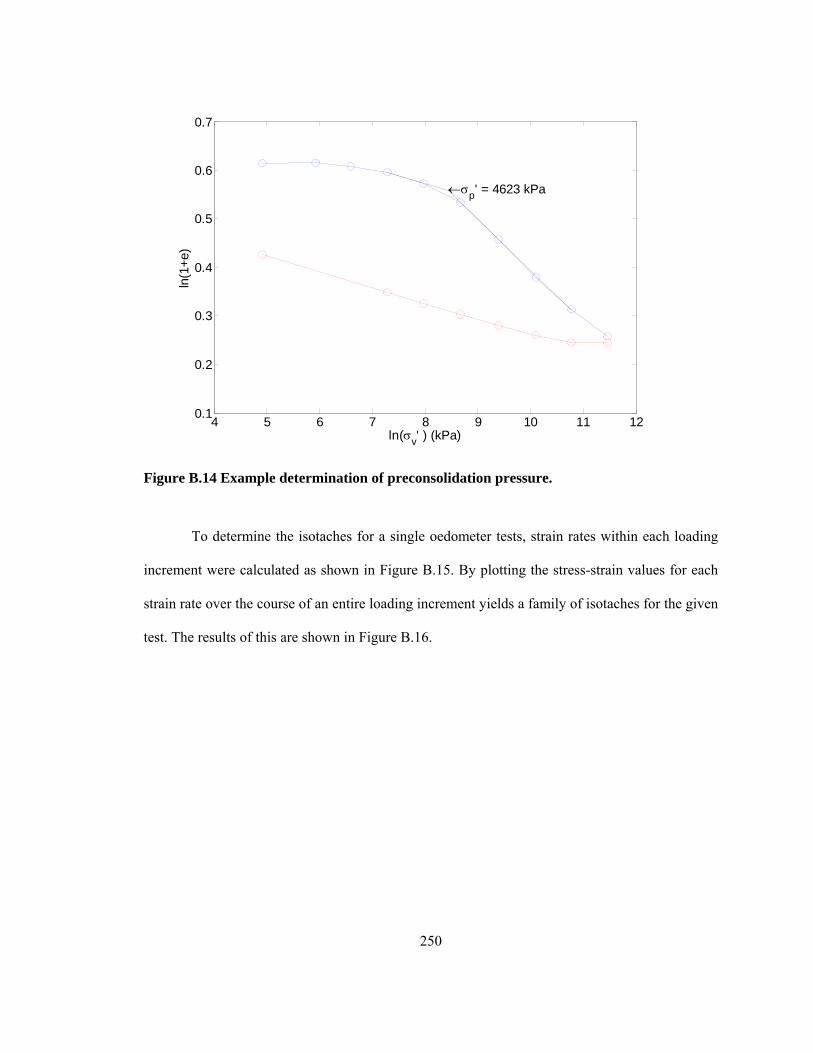
250
4 5 6 7 8 9 10 11 120.1
0.2
0.3
0.4
0.5
0.6
0.7
←σp' = 4623 kPa
ln(σv' ) (kPa)
ln(1
+e)
Figure B.14 Example determination of preconsolidation pressure.
To determine the isotaches for a single oedometer tests, strain rates within each loading
increment were calculated as shown in Figure B.15. By plotting the stress-strain values for each
strain rate over the course of an entire loading increment yields a family of isotaches for the given
test. The results of this are shown in Figure B.16.
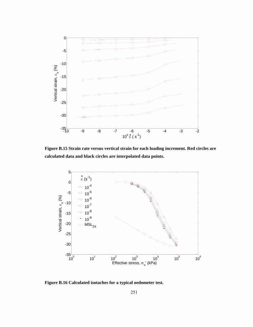
251
-10 -9 -8 -7 -6 -5 -4 -3 -2-35
-30
-25
-20
-15
-10
-5
0
Ver
tical
stra
in, ε
v (%)
10x ε ( s-1)
Figure B.15 Strain rate versus vertical strain for each loading increment. Red circles are
calculated data and black circles are interpolated data points.
100
101
102
103
104
105
106-35
-30
-25
-20
-15
-10
-5
0
5
Effective stress, σv' (kPa)
Ver
tical
stra
in, ε
v (%)
10-4
10-5
10-6
10-7
10-8
10-9
MSL24
ε (s-1)
Figure B.16 Calculated isotaches for a typical oedometer test.

252
B.7CRS Test Data
As described earlier data for the CRS tests were collected in a data acquisition system.
The interval on which the data was recorded varied based on the speed at which the test was
conducted. Measurements varied from every minute to every 3 minutes. Due to the large amounts
of data collect the individual test data is not presented however the pre and post test
measurements are presented below. Table B.1 provides a testing matrix for all tests conducted.
Table B.1 CRS Testing Matrix
Sample ID Depth (m)
Diameter of Specimen
(mm)
Frame loading rate
(mm/min)
Strain rate (s-1)
169US_0008 16.9 0.0008 1.64E-06 169US_00008 41.90 – 42.43 16.9 0.00008 1.46E-07 202US_0008 16.9 0.0008 1.40E-06
202US_00008 90.79-91.15 16.9 0.00008 1.51E-07
B.8CRS Test Results
Due to the number of tests conducted only one set of typical test results for a CRS test are
shown below however data analysis for tests shown in Table B.1 was conducted in this manner.
Displacement, load and pore pressure readings versus time for a typical test are shown in Figure
B.17. Stress-strain summary plots for a typical CRS are presented in Figure B.18.
Preconsolidation pressure determination was performed using the Butterfield method (Chapter 2)
as shown in Figure B.19.

253
5 5.5 6 6.5 7 7.5 8x 10
4
-5
0
5
Dis
plac
emen
t (m
m)
5 5.5 6 6.5 7 7.5 8x 10
4
0
10
20
Load
(kN
)
5 5.5 6 6.5 7 7.5 8x 10
4
0
20
40
Por
e P
ress
ure
(kP
a)
Time (s)
Figure B.17 Data outputs from data acquisition system for a typical CRS test.
102
103
104
105-30
-20
-10
0
10
Verti
cal S
train
, εv (%
)
Effective stress, σv' (kPa)
102
103
104
1050.2
0.4
0.6
0.8
1
Void
ratio
, e
Effective stress, σv' (kPa)
Figure B.18 Summary plots for a typical CRS test.

254
6 7 8 9 10 11 120.2
0.25
0.3
0.35
0.4
0.45
0.5
←9072 kPa
ln(σv') (kPa)
ln(1
+e)
Figure B.19 Preconsolidation pressure determination for CRS data.

Appendix C
C.1Triaxial Swell Test - Sensor Calibration
Each triaxial swell test contained 4 radial LVDTs, one axial LVDT, and two pressure
transducers (one measuring water pressure and one measuring cell pressure). Each of the sensors
was calibrated prior to any tests being conducted, the results of which are presented below.
Cell 1 - Radial LVDT_A
y = 7130.9x - 26196R2 = 0.9988
-30000-25000-20000-15000-10000-5000
05000
1000015000
0 1 2 3 4 5 6
Displacement (mm)
Rea
ding
(V)
LVDT_A (radial) Series2 Linear (LVDT_A (radial))
Cell 1 - Radial LVDT_B
y = 6721x - 20383R2 = 0.9986
-25000-20000-15000-10000-5000
05000
1000015000
0 1 2 3 4 5 6
Displacement (mm)
Rea
ding
(V)
LVDT_B Series2 Linear (LVDT_B)

256
Cell 1 - Radial LVDT_C
y = 7303.2x - 24457R2 = 0.9997
-30000-25000-20000-15000-10000-5000
05000
1000015000
0 1 2 3 4 5 6
Displacement (mm)
Rea
ding
(V)
LVDT_C Series2 Linear (LVDT_C)
Cell 1 - Radial LVDT_D
y = 6960x - 25583R2 = 0.9989
-30000-25000-20000-15000-10000-5000
05000
1000015000
0 1 2 3 4 5 6
Displacement (mm)
Rea
ding
(V)
LVDT_D Series2 Linear (LVDT_D)

257
Cell 1 - Axial LVDT
y = 1664.9x - 24241R2 = 0.9998
-30000
-20000
-10000
0
10000
20000
30000
0 5 10 15 20 25 30
Displacement (mm)
Rea
ding
(V)
LVDT_Axial Series2 Linear (LVDT_Axial)
Cell 1 - Water Pressure
y = 28.596x - 29051R2 = 1
-40000
-30000
-20000
-10000
0
10000
20000
0 500 1000 1500 2000
Applied Pressure (kPa)
Rea
ding
(V)
Water Pressure Series2 Linear (Water Pressure)
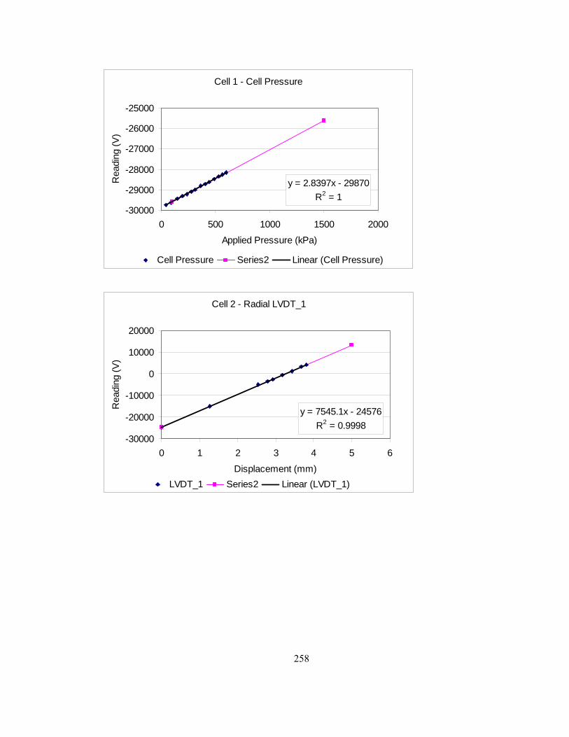
258
Cell 1 - Cell Pressure
y = 2.8397x - 29870R2 = 1
-30000
-29000
-28000
-27000
-26000
-25000
0 500 1000 1500 2000
Applied Pressure (kPa)
Rea
ding
(V)
Cell Pressure Series2 Linear (Cell Pressure)
Cell 2 - Radial LVDT_1
y = 7545.1x - 24576R2 = 0.9998
-30000
-20000
-10000
0
10000
20000
0 1 2 3 4 5 6
Displacement (mm)
Rea
ding
(V)
LVDT_1 Series2 Linear (LVDT_1)

259
Cell 2 - Radial LVDT_2
y = 7697x - 23820R2 = 0.9997
-30000
-20000
-10000
0
10000
20000
0 1 2 3 4 5 6
Displacement (mm)
Rea
ding
(V)
LVDT_2 Series2 Linear (LVDT_2)
Cell 2 - Radial LVDT_3
y = 7109.6x - 26643R2 = 0.9998
-30000
-20000
-10000
0
10000
20000
0 1 2 3 4 5 6
Displacement (mm)
Rea
ding
(V)
LVDT_3 Series2 Linear (LVDT_3)

260
Cell 2 - Radial LVDT_4
y = 7498.5x - 24257R2 = 0.9994
-30000
-20000
-10000
0
10000
20000
0 1 2 3 4 5 6
Displacement (mm)
Rea
ding
(V)
LVDT_4 Series2 Linear (LVDT_4)
Cell 2 - Axial LVDT
y = 1636x - 24234R2 = 0.9999
-30000
-20000
-10000
0
10000
20000
0 5 10 15 20 25 30
Displacement (mm)
Rea
ding
(V)
LVDT_Axial Series2 Linear (LVDT_Axial)

261
Cell 2 - Water Pressure
y = 28.597x - 29764R2 = 1
-40000
-30000
-20000
-10000
0
10000
20000
0 500 1000 1500 2000
Applied Pressure (kPa)
Rea
ding
(V)
Water Pressure Series2 Linear (Water Pressure)
Cell 2 - Cell Pressure
y = 2.8643x - 29403R2 = 1
-30000
-29000
-28000
-27000
-26000
-25000
-24000
0 500 1000 1500 2000
Applied Pressure (kPa)
Rea
ding
(V)
Cell Pressure Series2 Linear (Cell Pressure)

Appendix D
D.1Model Development
The model discussed in Chapter 4 is comprised of 4 linked stages, a SEEP/W stage
followed by three CTRAN/W stages. The SEEP/W solves the groundwater seepage analysis in
the first stage. This is followed by CTRAN/W stages where solute transport is determined. The
second stage sets the initial concentration conditions within the different materials. The third
stage reflects the period of time during glaciation and the forth stage represents the period of time
since deglaciation and introduction of modern day precipitation. The model geometry and
material properties remain constant throughout each stage of the model, it is only the boundary
conditions during the two time dependent stages (three and four) that are altered in each
subsequent stage. Material properties and model setup will be discussed here, however the details
of the applied boundary conditions are outlined in the Chapter 4.
The first stage in the modeling was to create a SEEP/W model. The model set up
consisted of a single column separated into the appropriate field site stratigraphy. Details of the
model geometry are site specific as discussed in Chapter 4, however for the purposes of this
discussion the Luck Lake model will be used. The overall geometry of the model is a column 120
m in length consisting of 30 m of glacial till overlying 90 m of clay, as shown in Figure D.1 (a).
The model is meshed with 1 m spacing as show in Figure D.1 (b). Volumetric water content,
density and hydraulic conductivity are the required material properties for the SEEP/W model.
Volumetric water content and density for the till were determined by Remenda (1993) and found
to be 0.31 and 1.87 Mg/m3, respectively. Values for the clay were determined from cores samples
and found to be 0.4 and 1.66 Mg/m3, respectively. These values are consistent with those found
by Shaw (1997) at the nearby King site. Measured hydraulic gradients, from the recorded water
levels, in the till and clay were found to be 0.014 and 0.2, respectively. Average linear

263
groundwater velocities on site have been measured at values up to 3 m per 10,000 years
(Remenda 1993). Slug tests performed after piezometers installation on site yielded hydraulic
conductivity values in the till that range from 4x10⁻¹⁰ m/s to 3x10-11 m/s. Result from oedometer
tests (Appendix B) indicate hydraulic conductivity values of the clay are on the order of 10-12 m/s.
Neuzil (1994) reported hydraulic conductively values ranging from 5x10-14 m/s to 5x10-12 m/s on
core samples from Cretaceous shale in North Dakota that can be stratigraphically correlated to the
Snakebite member of the Bearpaw shale. Shaw and Hendry (1998) reported hydraulic
conductivities values in the Snakebite member to be 4.4x10⁻¹² m/s to 5.3x10⁻¹² m/s. These
estimates of hydraulic conductivity, along with the measured gradients at the site suggest that
average Darcy velocities range from 0.01 to 1.8 m per 10,000 years. Boundary conditions for the
seepage analysis consist of flux or head boundary measurements. Based on the calculated Darcy
velocities, a constant flux boundary was place on the top of the column and a constant head
boundary was applied to the base of the model as seen in Figure D.2. The rate of flux used ranged
from 0 (diffusion only) to 1.5 m per 10,000 years to encompass the range of hydraulic
conductivity found within the materials. For each model and specified flux, resultant bulk and
individual hydraulic conductivity values for the different material were calculated and used as the
material inputs. The constant head boundary applied to the base of the model was 50 mbgs as
recorded by others in the underlying aquifer (Shaw and Hendry, 1998). To ensure internal
consistency within the model resulting from the constant flux boundary condition applied, the
input hydraulic correspond to the input flux boundary conditions to ensure the water table is set at
the top of the model, which corresponds to 2 m below ground surface and the average elevation
of the water table.
The second stage of the model is a CTRAN/W model sets the initial deuterium
concentration. Material properties in the CTRAN/W model are based on the solute movement
parameters consisting of effective diffusion and diffusivity. The effective diffusion coefficient for

264
deuterium within these materials has been examined by a number of researchers (Remenda et al.,
1996; Hendry and Wassenaar, 1999; van der Kamp et al., 1996) and in each case determined that
De to be the same for both the clay and till of 1.7x10⁻¹⁰m2/s, which was subsequently used in this
modeling. More recently Reiffereshield (2007) found that the effective diffusion coefficient with
the Battleford till to be 3.5 x10⁻¹⁰m2/s. This alternate diffusion coefficient was used in refinement
of the model parameters discussed in Chapter 4. Taking a conservative approach a δD of -178‰
was applied to the till as it initial boundary condition, uniformly over the entire region as shown
in Figure D.3a. The consistent δD value of -142‰ in the clay below 70 m suggests a uniform
distribution throughout the clay. It was therefore assumed that at the onset of glaciation the δD
profile in the clay was consistent and uniform at -142‰ as shown in Figure D.3a.
The final two CTRAN/W stages in the model deal with the timing and processes of
different geologic events that are being examined. The third stage of the model represents the
time during glaciation in which the material was covered in ice. Radiocarbon dating of material
between the Battleford and Floral Formations range between 189 and 38 ka (Christiansen, 1971)
indicating the Battleford Formation was deposited after this. The Floral Formation however is
estimated to be greater than 128kPa. Based on these results the time period for the ice cover stage
of the model was constrained to within these two large time periods. During this stage the
boundary conditions were modified through a series of model scenarios however for the purpose
of this discussion the boundary conditions were as follows. The concentration at the top of the till
was set to a consistent δD value of -178‰ reflecting the presence of melt water. The
concentration at the base of the clay was set to a δD value of -142‰ reflecting the constant
concentration of the underlying aquifer as shown in Figure D.3b.
The final model stage reflects the time since deglaciation which in southern
Saskatchewan occurs between 10,000 and 12,000 BP (Christiansen, 1979). During this stage of
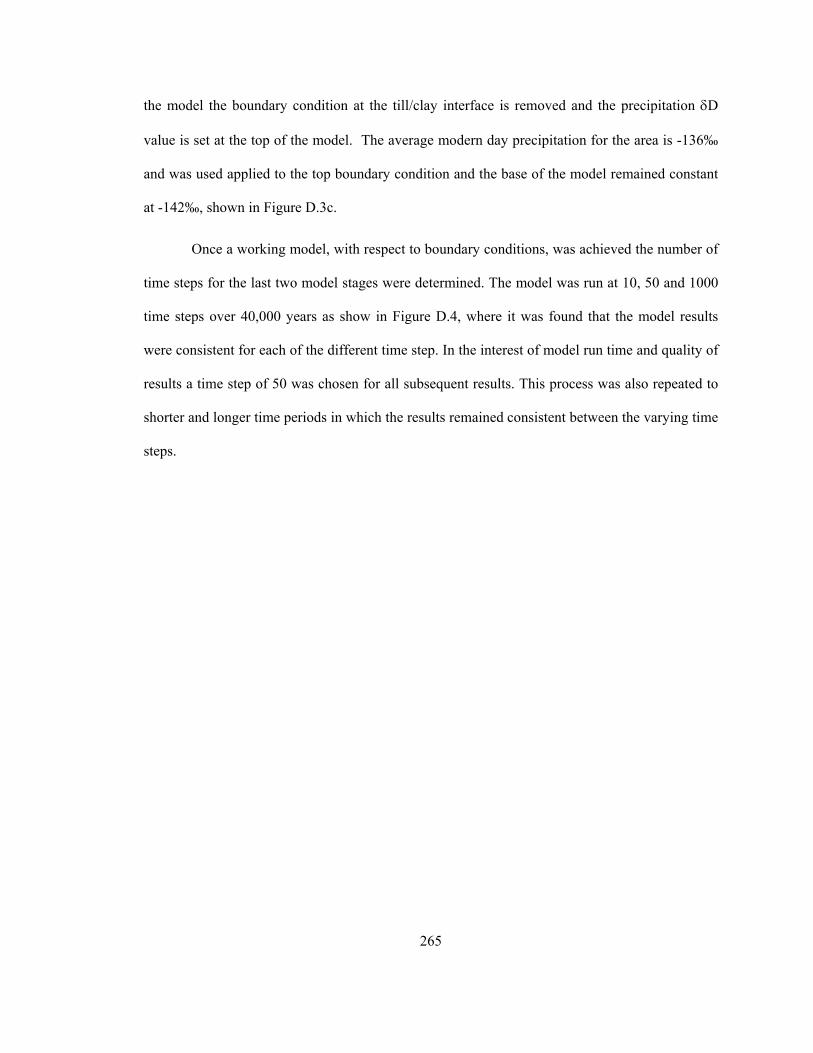
265
the model the boundary condition at the till/clay interface is removed and the precipitation δD
value is set at the top of the model. The average modern day precipitation for the area is -136‰
and was used applied to the top boundary condition and the base of the model remained constant
at -142‰, shown in Figure D.3c.
Once a working model, with respect to boundary conditions, was achieved the number of
time steps for the last two model stages were determined. The model was run at 10, 50 and 1000
time steps over 40,000 years as show in Figure D.4, where it was found that the model results
were consistent for each of the different time step. In the interest of model run time and quality of
results a time step of 50 was chosen for all subsequent results. This process was also repeated to
shorter and longer time periods in which the results remained consistent between the varying time
steps.
266
(a) (b)
Figure D.1 (a) Luck Lake model geometry and (b) 1m spaced meshed model
Till
Clay

267
(a) (b)
Figure D.2 (a) SEEP/W model boundary conditions (b) Pressure head results showing water
table at 2m below ground surface.
Constant flux, q
Constant head
50 mbgs
10
20
30
40
50
60
70

268
(a) (b) (c)
Figure D.3 CTRAN/W stages and boundary conditions (a) Initial material concentrations
(b) Stage 3 boundary conditions (initial) and (b) Stage 4 boundary conditions (initial).
-142 ‰
-178 ‰
-136 ‰
-142 ‰
-142 ‰
-178 ‰

269
Figure D.4 Time step determination for the model.

270
Appendix E
E.1Core Sampling & Preservation
Two types of core samples were collected during this research, Shelby tubes and Denison
core barrels. The Shelby tubes were 0.76 mm in diameter and 0.6 m in length and the Denison
core barrels were 0.76 mm diameter and 1.5 m in length.
Upon retrieval of the core samples the ends of the tubes were sealed with wax to prevent
moisture loss throughout the reminder of the field investigation. Once the investigation was
complete the core samples were returned to a laboratory and extruded. The core samples collected
during the 2005 investigation were taken to the University of Saskatchewan Soils Laboratory
where they were extruded. The core samples collected during the 2006 investigation were taken
to the Saskatchewan Department of Highways material testing laboratory in Regina for extrusion.
To extrude the samples, the core barrels were placed horizontally against a hydraulic piston. The
hydraulic piston then pushes the sample out of the core barrel from one end. The extruded sample
was collected in half of a PVC tube as shown in Figure E.1. Following extrusion, the condition of
the core sample was inspected. Once the visual inspection was complete, the cores were wrapped
in plastic wrap followed by masking tape. The final step in preserving the moisture content was to
coat the cores samples in wax (Figure E.2).
Transportation of the core samples from Saskatchewan to Ontario was done through
courier service. The wax and sealed cores were packed in bubble wrap and styroform before
being placed in a hard plastic container for shipping. Once the samples arrived in Ontario they
were stored in a cold room at approximately 4oC for the duration of the research. Each time
specimens were taken from the cores, the remaining cores were re-sealed and placed back in the
cold room.

271
Figure E.1 Hydraulic piston core sample extruded.
Figure E.2 Sealed and waxed core samples.
Hydraulic piston