Geostatistical modelling on stream networks: developing valid ...

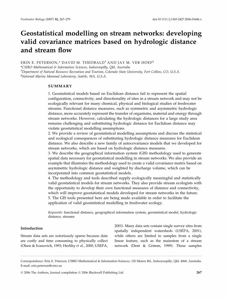
Geostatistical modelling on stream networks: developingvalid covariance matrices based on hydrologic distanceand stream flow

ERIN E. PETERSON,* DAVID M. THEOBALD† AND JAY M. VER HOEF ‡

*CSIRO Mathematical & Information Sciences, Indooroopilly, Qld, Australia†Department of Natural Resource Recreation and Tourism, Colorado State University, Fort Collins, CO, U.S.A.‡National Marine Mammal Laboratory, Seattle, WA, U.S.A.

SUMMARY

1. Geostatistical models based on Euclidean distance fail to represent the spatial

configuration, connectivity, and directionality of sites in a stream network and may not be

ecologically relevant for many chemical, physical and biological studies of freshwater

streams. Functional distance measures, such as symmetric and asymmetric hydrologic

distance, more accurately represent the transfer of organisms, material and energy through

stream networks. However, calculating the hydrologic distances for a large study area

remains challenging and substituting hydrologic distance for Euclidean distance may

violate geostatistical modelling assumptions.

2. We provide a review of geostatistical modelling assumptions and discuss the statistical

and ecological consequences of substituting hydrologic distance measures for Euclidean

distance. We also describe a new family of autocovariance models that we developed for

stream networks, which are based on hydrologic distance measures.

3. We describe the geographical information system (GIS) methodology used to generate

spatial data necessary for geostatistical modelling in stream networks. We also provide an

example that illustrates the methodology used to create a valid covariance matrix based on

asymmetric hydrologic distance and weighted by discharge volume, which can be

incorporated into common geostatistical models.

4. The methodology and tools described supply ecologically meaningful and statistically

valid geostatistical models for stream networks. They also provide stream ecologists with

the opportunity to develop their own functional measures of distance and connectivity,

which will improve geostatistical models developed for stream networks in the future.

5. The GIS tools presented here are being made available in order to facilitate the

application of valid geostatistical modelling in freshwater ecology.

Keywords: functional distance, geographical information system, geostatistical model, hydrologicdistance, streams

Introduction

Stream data sets are notoriously sparse because data

are costly and time consuming to physically collect

(Olsen & Ivanovich, 1993; Herlihy et al., 2000; USEPA,

2001). Many data sets contain single survey sites from

spatially independent watersheds (USEPA, 2001),

while others are limited to samples from a single

linear feature, such as the mainstem of a stream

network (Dent & Grimm, 1999). These samples

Correspondence: Erin E. Peterson, CSIRO Mathematical & Information Sciences, 120 Meiers Rd., Indooroopilly, Qld, 4068, Australia.

E-mail: [email protected]

Freshwater Biology (2007) 52, 267–279 doi:10.1111/j.1365-2427.2006.01686.x

� 2006 The Authors, Journal compilation � 2006 Blackwell Publishing Ltd 267

provide valuable information about the ecological

condition at distinct points, but may not provide all of

the information necessary to investigate processes and

interactions at a network or regional-scale.

Recently, researchers have recognised that some

principle themes in landscape ecology, such as

hierarchy theory, may also be relevant in freshwater

ecology (Fausch et al., 2002; Ward et al., 2002; Wiens,

2002). This trend has sparked an exciting new set of

research questions, which are related to multi-scale

biological, ecological and physical processes, such as

habitat utilisation by aquatic species (Kneib, 1994). It

is difficult to recognise multi-scale patterns in a

freshwater environment based on sparse site-scale

data and it is prohibitively costly to collect a continu-

ous regional sample throughout space. Therefore, we

propose that geostatistical models be used to investi-

gate spatial patterns in streams data and to make

predictions throughout stream networks.

Geostatistical models are commonly used to quan-

tify spatial patterns in the terrestrial environment, but

have been applied less frequently to aquatic systems

such as lakes (Altunkaynak, Ozger & Sen, 2003),

estuaries (Little, Edwards & Porter, 1997; Rathbun,

1998), and streams (Kellum, 2002; Yuan, 2004).

Freshwater ecologists might have found little utility

in geostatistical models because they are typically

based on Euclidean (also known as straight-line)

distance. Euclidean distance may not be ecologically

meaningful because it fails to represent the spatial

configuration, connectivity, directionality and relative

position of sites in a stream network. Therefore, it

may not be a suitable distance measure for most

chemical, physical and biological studies of fresh-

water streams (Olden, Jackson & Peres-Neto, 2001;

Benda et al., 2004; Ganio, Torgersen & Gresswell,

2005). Recently, freshwater ecologists have begun to

explore spatial patterns in stream networks using

hydrologic distance measures (Dent & Grimm, 1999;

Gardner, Sullivan & Lembo, 2003; Legleiter et al.,

2003; Torgersen, Gresswell & Bateman, 2004; Ganio

et al., 2005). In addition, new geostatistical methodol-

ogies have recently been developed that rely on valid

covariances based on directional hydrologic distance

measures (Cressie et al., 2006; Ver Hoef, Peterson &

Theobald, 2006). This provides ecologists with a

variety of distance measures to choose from and

makes geostatistical modelling an ecologically rele-

vant tool.

Our objective is to discuss and demonstrate meth-

ods used to create valid covariance matrices based on

hydrologic distance measures. Geostatistical model-

ling assumptions are reviewed and the statistical

consequences of substituting hydrologic distance

measures for Euclidean distance will be explained.

We also describe a methodology to generate a valid

covariance matrix based on asymmetric hydrologic

distance weighted by discharge volume.

Background

Distance measures for use in geostatistical models

Two types of distances are often used to represent

physical and ecological processes in stream ecosys-

tems: symmetric and asymmetric distance classes.

These distances are used to model connected sites that

have a quantifiable influence upon one another.

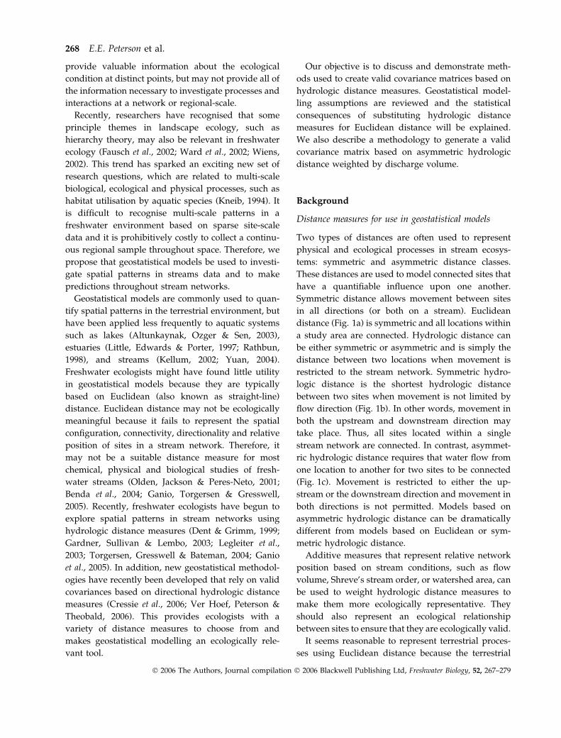
Symmetric distance allows movement between sites

in all directions (or both on a stream). Euclidean

distance (Fig. 1a) is symmetric and all locations within

a study area are connected. Hydrologic distance can

be either symmetric or asymmetric and is simply the

distance between two locations when movement is

restricted to the stream network. Symmetric hydro-

logic distance is the shortest hydrologic distance

between two sites when movement is not limited by

flow direction (Fig. 1b). In other words, movement in

both the upstream and downstream direction may

take place. Thus, all sites located within a single

stream network are connected. In contrast, asymmet-

ric hydrologic distance requires that water flow from

one location to another for two sites to be connected

(Fig. 1c). Movement is restricted to either the up-

stream or the downstream direction and movement in

both directions is not permitted. Models based on

asymmetric hydrologic distance can be dramatically

different from models based on Euclidean or sym-

metric hydrologic distance.

Additive measures that represent relative network

position based on stream conditions, such as flow

volume, Shreve’s stream order, or watershed area, can

be used to weight hydrologic distance measures to

make them more ecologically representative. They

should also represent an ecological relationship

between sites to ensure that they are ecologically valid.

It seems reasonable to represent terrestrial proces-

ses using Euclidean distance because the terrestrial

268 E.E. Peterson et al.

� 2006 The Authors, Journal compilation � 2006 Blackwell Publishing Ltd, Freshwater Biology, 52, 267–279

landscape is commonly represented as a two-dimen-

sional surface where any two sites may be connected.

At times, it may also be appropriate to apply Euclid-

ean distance to stream ecosystems. For example, an

aquatic response variable may be significantly influ-

enced by a continuous landscape variable, such as

geology type (Kellum, 2002) or by broad-scale factors,

such as acid precipitation (Driscoll et al., 2001).

We recognise that freshwater systems have four

dimensions: longitudinal (along the flow line), lateral

(across the flow line), vertical (depth), and temporal

(Ward, 1989), but we focus solely on the longitudinal

dimension. In this case, a two-dimensional represen-

tation of distance may not always be appropriate as

streams are represented as linear features and typic-

ally the movement of material is strongly influenced

by unidirectional flow. For example, some fish move

both up and downstream, but cannot move across the

terrestrial landscape. Other materials, such as seeds or

chemicals, are passive movers primarily affected by

longitudinal transport. In these cases, movement is

restricted to the network, but occurs primarily in the

downstream direction.

The relative position in the network also affects the

condition of a site (Pringle, 2001; Benda et al., 2004)

and reflects the influence that it will have on other

sites (Cumming, 2002). For instance, a site located on a

small tributary may have little influence on a down-

stream site located on the mainstem because of

substantial differences in discharge volume (Benda

et al., 2004). Clearly, physical characteristics of the

stream network provide a vast amount of information

about conditions at unobserved sites and therefore,

functional distances based on hydrology should also

be considered.

Geostatistical modelling in stream networks

Linear statistical models traditionally have two com-

ponents: the deterministic mean (also known as trend)

and random errors, which are usually assumed to be

normally distributed, homoscedastic (constant vari-

ance), and independent, so that a random error at one

site is not influenced by that of another site. Streams

data commonly violate the assumption of independ-

ence as stream networks are hierarchically structured,

with nested watersheds, and stream segments that are

connected by flow. Geostatistical models can be seen

as a generalisation of traditional linear statistical

models with a deterministic mean function; however,

they relax the assumption of independence and allow

spatial autocorrelation in the errors (Ver Hoef et al.,

2001). Local deviations from the mean are modelled

using the covariance between nearby sites. The mean,

variance and autocorrelation structure of the error

term are assumed to be stationary or similar across a

study area (Cressie, 1993).

The covariance represents the strength of spatial

autocorrelation between two sites given their separ-

ation distance (h) (Olea, 1991). The separation distance

is simply the distance travelled from one location to a

second location and can be calculated using a variety

of distance measures. The covariance is the joint

variation of the values (Y(si), Y(sj)) at two locations

(si, sj) about their means (l(si), l(sj)) and provides a

quantitative measure of the way sites co-vary in space.

(c)

Symmetric distance classes Asymmetric distance classes

(a) (b)

1 2

3

1 2

3

1 2

3

Fig. 1 Symmetric and asymmetric distance classes. The stream network is represented by a solid line, while distance measurements

are represented with dotted lines. Symmetric hydrologic distance measures include Euclidean distance (a) and symmetric hydrologic

distance (b). Sites 1, 2, and 3 are all neighbours to one another when these distance measures are used. Asymmetric distance classes

include upstream and downstream asymmetric hydrologic distance (c). Sites 1 and 2 are neighbours to site 3, but not to each other.

Valid autocovariance models for stream networks 269


The covariance of a spatial stochastic process {Y(s),

s 2 R} at any two locations within a study area (R) is

defined as:

Cðsi; sjÞ ¼ E YðsiÞ � lðsiÞ½ � YðsjÞ � lðsjÞ� ��

; ð1Þ

where E(Æ) represents the expectation (Bailey &

Gatrell, 1995).

There are more covariances than data in (Eqn 1)

because we cannot observe a response continually in

space. Therefore, we make simplifying assumptions

by using an autocovariance function, which typically

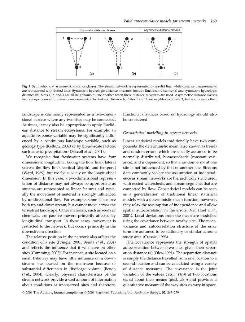
has three parameters (h), the nugget effect, sill and

range. These must be estimated in order to fit the

function to the empirical covariances (Fig. 2). The

nugget effect represents the variation between sites as

their separation distance approaches zero. It can result

from experimental error or could indicate that a

substantial amount of variation occurs at a scale finer

than the sampling scale. The autocovariance asymp-

tote is called the sill and it represents variance found

among uncorrelated data. The range parameter des-

cribes how fast the autocovariance decays with

distance. Some common methods that can be used

to estimate the autocovariance parameters include

maximum likelihood, restricted maximum likelihood

(REML), weighted least-squares (Cressie, 1993), or

Markov Chain Monte Carlo in a Bayesian framework

(Handcock & Stein, 1993). The mathematical structure

of the fitted autocovariance function provides a way

to estimate the local deviation from the mean value at

an unobserved site using observed values at nearby

sites. Thus, geostatistical models are typically able to

model more variability in the response variable and

provide more accurate predictions at unobserved sites

when spatial autocorrelation is present in the data

(Isaaks & Srivastava, 1989).

In general, covariance matrices contain the covar-

iance between each site and every other site. They

have n rows and n columns, where n is the total

number of sample sites. In geostatistics, these covar-

iances are obtained from the fitted autocovariance

function. Not all functions are valid because the

covariance matrix must be symmetric, positive-defi-

nite, and all diagonal elements must be non-negative

(Cressie, 1993). However, a review of methods used to

examine these assumptions is beyond the scope of this

manuscript. See Isaaks & Srivastava (1989) for a

detailed discussion of positive-definite matrices and

rules used to test them.

A few notable efforts have used symmetric hydro-

logic distance to explore spatial autocorrelation in

stream networks. Their results indicate that patterns

of spatial autocorrelation in biological (Torgersen

et al., 2004; Ganio et al., 2005), chemical (Dent &

Grimm, 1999; Gardner et al., 2003), and physical

(Legleiter et al., 2003) streams data can be represented

using symmetric hydrologic distance. However, the

exponential model is the only known autocovariance

function that is valid when making predictions at

unobserved locations using covariance matrices based

on symmetric hydrologic distance (Ver Hoef et al.,

2006). When symmetric hydrologic distance is substi-

tuted for Euclidean distance in other commonly used

geostatistical autocovariance functions, the covariance

matrix may contain negative eigenvalues, it may

produce negative variance estimates, it is not guaran-

teed to be positive-definite, and therefore it is not

valid. To our knowledge, there have been no valid

predictions generated using geostatistical models

solely based on symmetric hydrologic distance meas-

ures.

An asymmetric hydrologic distance measure may

more accurately characterise passive movement in

riverine systems because ecological and physical

stream processes are strongly influenced by network

configuration and flow direction (Olden et al., 2001;

Fagan, 2002). However, pure asymmetric distance

measures (unweighted) do not produce symmetric

covariance matrices, which are required for geostatis-

tical modelling. Here we describe how to generate

valid covariance matrices based on a weighted asym-

metric hydrologic distance (WAHD). These should be

ecologically interesting because they more accurately

Separation distance

Cov

aria

nce

Sill

Nugget effect

Range

100000

10

Bin

Fig. 2 Covariograms are generated by grouping the separation

distances into bins, calculating a mean covariance for each bin,

and plotting them in ascending order. Each mean covariance is

represented by a single point. The covariogram is used to derive

visual estimates of the nugget, range and sill.



represent the connectivity and flow relationships in

stream networks, and they provide a useful tool for

geostatistical modelling in stream networks. Next, we

develop spatial autocovariance models using moving

average constructions based on asymmetric hydro-

logic distances that are both statistically and ecologic-

ally valid for stream networks (Cressie et al., 2006; Ver

Hoef et al., 2006).

Autocovariance models using hydrologic distances

Stream processes and conditions are not necessarily

random in an ecological sense because they result

from ecologically complex interactions; however, we

model our lack of knowledge about such processes

with random variables. In that sense, a single stream

sample is one realisation from a distribution of

possible sample values, but that sample can have

autocorrelation among its values. Our goal is to create

autocorrelated models for stream networks. Barry &

Ver Hoef (1996) show that a large class of autocovar-

iance functions can be developed by creating random

variables as the integration of a moving average

function over white noise random process:

ZðsÞ ¼Z 1�1

gðx� sjhÞWðxÞdx; ð2Þ

where W(x) is the white noise random process and

g(x)s|h) is the moving average function. The moving

average construction allows a valid autocovariance to

be expressed as:

CðhjhÞ ¼R1�1 gðxjhÞ½ �2dxþ h0 if h ¼ 0R1�1 gðxjhÞgðx� hjhÞdx if h > 0,

(ð3Þ

where h0 is the nugget effect and h is the separation

distance. We also assume that the integral exists. This

idea will now be developed for stream networks.

It is useful to establish a mathematical framework

and notation before describing the moving average

construction of a valid autocovariance model for

stream networks. For our purposes, a stream segment

is defined as a single line feature in a vector data set.

A group of segments with a common stream outlet, or

pour point, form a stream network. It is possible to

measure the distance upstream of any segment from

the stream outlet within a single network. We refer to

this as the ‘distance upstream.’ The outlet’s distance

upstream to itself is zero. The stream segments within

a network are indexed arbitrarily with i ¼ 1, 2, …, m.

We denote each location as xi, which is the distance

upstream on the ith stream segment, to uniquely

define each location. Similarly, we denote the most

downstream location on the ith segment as li, and the

most upstream location as ui, where ui is ¥ if there are

no stream segments upstream of the ith segment.

Stream segments within a network are connected and

therefore, li ¼ uj when the ith segment is directly

upstream from the jth segment. Let the index set of

stream segments upstream of xi, excluding i, be Uxi,

and let Bxi,sj

be the index set of segments between

downstream location xi and upstream location sj,

excluding the downstream segment but including the

upstream segment. In a similar way, let Bxi,[j] be the

index set between a downstream location and an

upstream segment j (for more details, see Ver Hoef

et al., 2006).

For the unique conditions in a stream network, a

moving average construction that is equivalent to

Eqn 2 is used to create the random variable Z(si) at

stream location si:

ZðsiÞ ¼Z ui

si

gðxi � sijhÞWðxiÞdxi

þXj2Usi

Yk2Bsi ;½j�

ffiffiffiffiffiffixkp

0@

1AZ uj

lj

gðxj � sijhÞWðxjÞdxj;

ð4Þ

where g(x|h) is the moving average function that

depends on parameters h. It can be non-zero for

positive values, but must be zero for all negative

values. W(xi) is the white noise process on the ith

stream segment and xk is a segment weight equal to

the proportion that a stream segment contributes to

the segment directly downstream. This general for-

mulation is given by Ver Hoef et al. (2006). If weights

on stream segments are a sum of the weights on the

two segments directly above it, a special case of Eqn 4

is given by Cressie et al. (2006). Special care has been

taken with the weights to ensure that all random

variables have the same variance, however such a

construction could allow for non-stationary variances.

An interpretation of Eqn 4 is that we construct the

random variable segment by segment, starting with

the ith segment and move upstream. However, as we

go upstream, the moving average function must

branch with each stream segment j. To keep a constant

variance, the moving average function must be

apportioned at each branch. The multiplication of



weights (between 0 and 1) ensures that influence

decreases as we move upstream, but we can also

control which branches have more influence through

the weights themselves.

We use the definition given in Eqn 4 to build valid

autocovariance models for stream networks:

and

C1ðhÞ ¼Z 1�1

gðxjhÞgðx� hjhÞdx;

where si and sj represent two spatial locations on

the stream network and |si)sj| is the hydrologic

distance between them. Once the asymmetric hydro-

logic distance data have been weighted appropriately,

the exponential, linear with sill, spherical, or Mariah

autocovariance functions (Ver Hoef et al., 2006) can be

fit to the empirical covariances using one of the

parameter estimation methods mentioned previously.

Ver Hoef et al. (2006) used REML for several models,

while Cressie et al. (2006), used weighted least squares

for a spherical autocovariance. A valid covariance

matrix produced using the moving average autoco-

variance functions can be used as input for a variety of

kriging equations, such as simple, ordinary, or uni-

versal kriging (Cressie, 1993; Bailey & Gatrell, 1995).

Moving average autocovariance functions for

stream networks are a new statistical development

and therefore, few geostatistical models based on

WAHD have been generated. Ver Hoef et al. (2006)

developed the methodology for the WAHD models

and provided an example using a spatially dense

subset of sulphate (meq L)1). Peterson et al. (2006)

used a large data set to compare patterns of spatial

autocorrelation in eight water chemistry variables:

dissolved oxygen, sulphate, nitrate-nitrogen, tempera-

ture, dissolved organic carbon, pH, acid-neutralising

capacity and conductivity, using three distance meas-

ures: Euclidean, symmetric hydrologic, and WAHD.

Cressie et al. (2006) developed a geostatistical model

for daily change in dissolved oxygen based on a

mixture of covariances, which is exciting because it

demonstrates how multiple patterns of spatial auto-

correlation can be represented in one geostatistical

model. For example, a broad-scale landscape process

that is not constrained by watershed boundaries, such

as the weathering of parent material or coarse climatic

conditions, might produce a primary pattern of spatial

autocorrelation that is better described using Euclid-

ean distance. In contrast, an instream process, such as

nutrient spiraling or fish movement, could produce a

secondary pattern at a different scale that may be

better described using a hydrologic distance measure.

GIS, hydrologic distances and spatial weights

The ability to generate covariance matrices based on a

moving average construction makes it possible to

create a variety of valid geostatistical models for

stream networks, but calculating distances and spatial

weights along stream networks remains challenging.

A handful of geographical information system (GIS)

tools have been developed to calculate hydrologic

distance, including the National Hydrography Dataset

(NHD) ARCVIEWARCVIEW Toolkit version 7.0 from the United

States Geological Survey (USGS, 2004a) and ARCARC

HYDROHYDRO Tools from the Environmental Systems Re-

search Institute (ESRI, 2001). However, each of these

tools has practical and theoretical limitations. The

NHD ARCVIEWARCVIEW Toolkit allows the user to calculate the

hydrologic distance between two sites based on flow

direction, but does not provide a tool to calculate the

spatial weights. The code is encrypted, which makes it

impossible to automate the tool so that processing

large data sets is difficult and time consuming. In

addition, the toolkit is not compatible with ESRI ARC-ARC-

GISGIS version 8.0 (ESRI, 2002) and higher. The ARCARC

HYDROHYDRO Tools can be used with more recent versions

of ARCGISARCGIS, but cannot be used to calculate the

hydrologic distance between sites or the spatial

weights without extensive data preprocessing and

programmatic modification. Other researchers have

developed their own scripts, written in AVENUEAVENUE, ARCARC

MACROMACRO Language, or VISUAL BASICVISUAL BASIC, to calculate the

hydrologic distance between sample sites (Rathbun,

1998; Theobald, 2002; Dussault & Brochu, 2003; Gard-

ner et al., 2003; Torgersen et al., 2004), but they were

Cðsi; sjjhÞ ¼

0 locations are not flow connected,C1ð0Þ þ h0 if location 1 = location 2,Qk2Bsi ;sj

ffiffiffiffiffiffixkp

C1 si � sj

�� otherwise.

8><>: ð5Þ



not designed to calculate the spatial weights for the

stream network. We believe that some practical and

accessible tools are needed to generate the hydrologic

distance matrices and spatial weights matrices in a

cost-efficient manner. Now we describe the methodo-

logy and tools in order to facilitate valid geostatistical

modelling in freshwater riverine systems.

Methods

We detail how to calculate a valid covariance matrix

based on asymmetric hydrologic distance and weigh-

ted by stream discharge. There are three steps: (i) data

preprocessing, (ii) generating the hydrologic distance

and spatial weights matrices, and (iii) creating a

statistically valid covariance matrix. We also provide

an example to illustrate these methods.

Preprocessing stream data

One challenge of working with GIS data is that sample

sites collected within a stream are not always located

directly on a stream segment, even though they

should be. This is a common phenomenon that can

result for a variety of reasons. Although GPS-based

points are differentially corrected, they still have some

error and do not always fall directly on a vertex or line

segment representing a stream. Some stretches of

river can move (e.g. meander) slightly from their

mapped position. Streams are often represented on a

map by lines and so samples collected on the banks of

a large river may not fall directly on a line segment.

When streams are represented at coarser scales the

digital streams data sets may contain mapping errors

and generalisations, such as the absence of small

tributaries and the homogenisation of form. Regard-

less of the error source, the sample sites must fall

exactly on a stream line. Our solution is to ‘snap’ the

sites to the nearest stream segment and manually

examine each site to ensure that it is located on the

correct stream segment. However, a refinement might

be to move the site to the nearest stream segment and

automatically compare attributes, such as stream

name or upstream watershed area, to ensure that it

lies in the correct location (Mixon, 2002). In contrast,

the NHD Reach Indexing Tool (USEPA, 2002) uses

dynamic segmentation to relate features to NHD

reaches without moving the feature or altering the

reach.

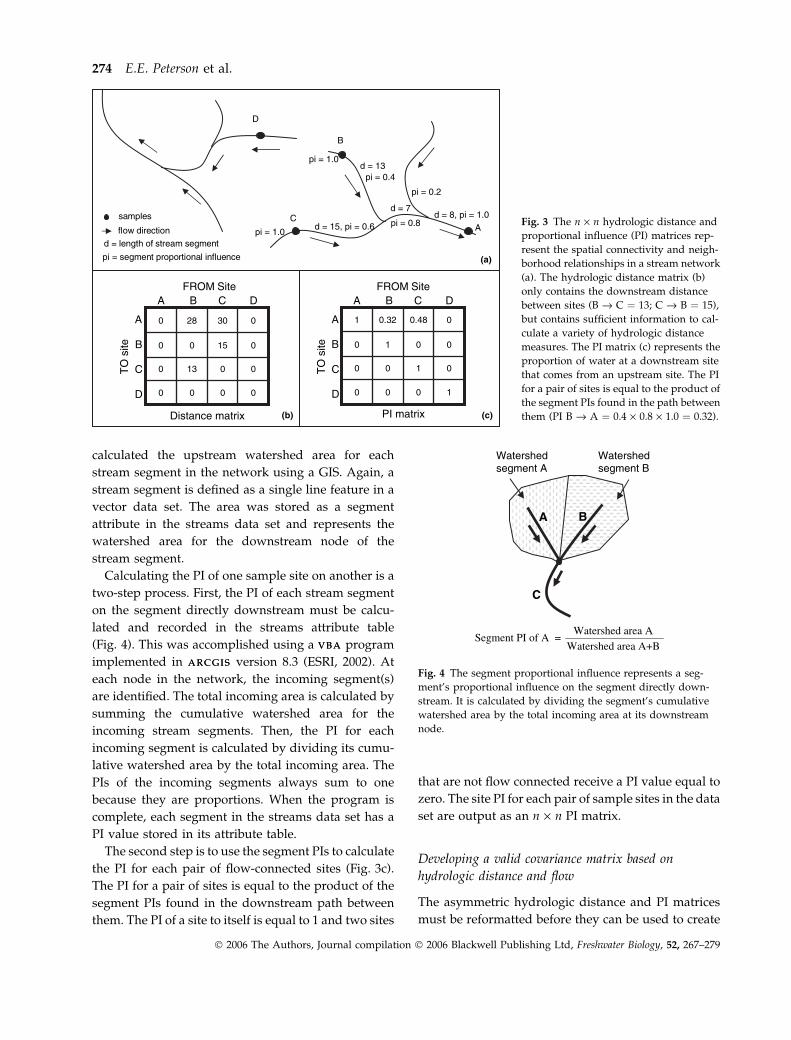
Calculating hydrologic distance measures

We developed a program in VISUAL BASICVISUAL BASIC Applica-

tions for ARCGISARCGIS version 8.3 (ESRI, 2002) to locate the

path between survey sites and to compute the hydro-

logic distance between geographical locations. The

total distance traversed in the downstream direction is

recorded in a distance table (Fig. 3b), which provides

sufficient information to calculate symmetric and

asymmetric hydrologic distance measures. Flow

direction is retained by recording the downstream

distance in both directions. For example, in Fig. 3a,b

the downstream distance from site B to site C ¼ 13

and the downstream distance from site C to site B ¼15. The upstream distance between two sites is found

by switching the direction of the path (e.g. upstream

distance from B to C ¼ 15 and upstream distance

from C to B ¼ 13). The symmetric hydrologic distance

is calculated by summing the two downstream

distances (e.g. B to C and C to B ¼ 13 + 15 ¼ 28).

Asymmetric hydrologic distance is restricted to flow-

connected sites, which are identified by comparing

the downstream distances between sites. If the dis-

tance is greater than zero in one direction and equal to

zero in the other, then the two sites are connected by

flow (e.g. downstream distance A to B ¼ 0 and

downstream distance B to A ¼ 28). They are not

connected by flow if the downstream distance is equal

to zero in both directions (e.g. D to A, D to B, D to C)

or the downstream distance is greater than zero in

both directions (e.g. B to C, C to B). The symmetric or

asymmetric hydrologic distance measures are calcu-

lated and recorded in an n · n hydrologic distance

matrix and output as a text file, which is compatible

with most statistical software.

Calculating the spatial weights

The proportional influence (PI) is defined as the

influence of an upstream location on a downstream

location and is used to create a spatial weights matrix.

It is based on discharge volume, which can be

calculated using regression equations (Vogel, Wilson

& Daly, 1999; USGS, 2004b) or process-based models

such as the Soil and Water Assessment Tool (Neitsch

et al., 2002). We use watershed area as a surrogate for

discharge, which appears to be a viable alternative as

it is correlated to mean annual discharge in every

region of the United States (Vogel et al., 1999). We



calculated the upstream watershed area for each

stream segment in the network using a GIS. Again, a

stream segment is defined as a single line feature in a

vector data set. The area was stored as a segment

attribute in the streams data set and represents the

watershed area for the downstream node of the

stream segment.

Calculating the PI of one sample site on another is a

two-step process. First, the PI of each stream segment

on the segment directly downstream must be calcu-

lated and recorded in the streams attribute table

(Fig. 4). This was accomplished using a VBAVBA program

implemented in ARCGISARCGIS version 8.3 (ESRI, 2002). At

each node in the network, the incoming segment(s)

are identified. The total incoming area is calculated by

summing the cumulative watershed area for the

incoming stream segments. Then, the PI for each

incoming segment is calculated by dividing its cumu-

lative watershed area by the total incoming area. The

PIs of the incoming segments always sum to one

because they are proportions. When the program is

complete, each segment in the streams data set has a

PI value stored in its attribute table.

The second step is to use the segment PIs to calculate

the PI for each pair of flow-connected sites (Fig. 3c).

The PI for a pair of sites is equal to the product of the

segment PIs found in the downstream path between

them. The PI of a site to itself is equal to 1 and two sites

that are not flow connected receive a PI value equal to

zero. The site PI for each pair of sample sites in the data

set are output as an n · n PI matrix.

Developing a valid covariance matrix based on

hydrologic distance and flow

The asymmetric hydrologic distance and PI matrices

must be reformatted before they can be used to create

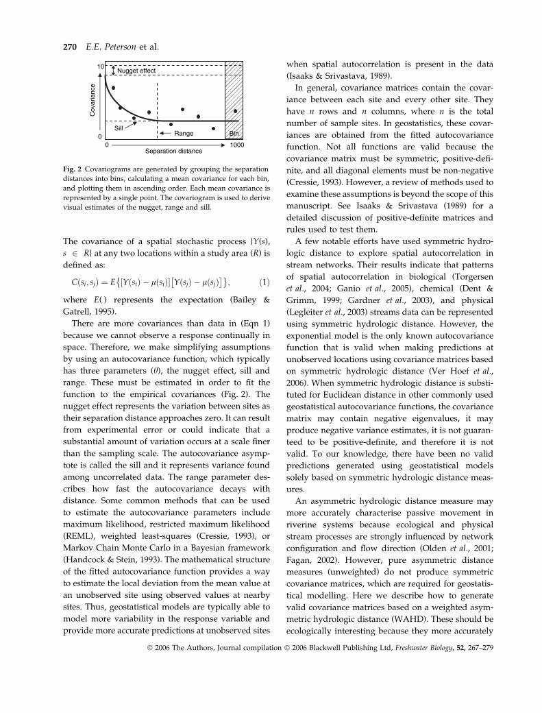
0000

00130

01500

030280

1000

0100

0010

00.480.321

D

B

A

d = 7

d = 13

d = 15, pi = 0.6d = 8, pi = 1.0 C

FROM Site

TO

site

TO

site

A

B

C

D

A C

pi = 0.2

pi = 1.0

pi = 1.0

pi = 0.4

pi = 0.8

FROM Site

A

B

C

D

Distance matrix PI matrix

(a)

(c)(b)

d = length of stream segment

samples

flow direction

pi = segment proportional influence

B D A CB D

Fig. 3 The n · n hydrologic distance and

proportional influence (PI) matrices rep-

resent the spatial connectivity and neigh-

borhood relationships in a stream network

(a). The hydrologic distance matrix (b)

only contains the downstream distance

between sites (B fi C ¼ 13; C fi B ¼ 15),

but contains sufficient information to cal-

culate a variety of hydrologic distance

measures. The PI matrix (c) represents the

proportion of water at a downstream site

that comes from an upstream site. The PI

for a pair of sites is equal to the product of

the segment PIs found in the path between

them (PI B fi A ¼ 0.4 · 0.8 · 1.0 ¼ 0.32).

BA

Watershed area ASegment PI of A =

Watershed area A+B

C

Watershed segment A

Watershed segment B

Fig. 4 The segment proportional influence represents a seg-

ment’s proportional influence on the segment directly down-

stream. It is calculated by dividing the segment’s cumulative

watershed area by the total incoming area at its downstream

node.



a statistically valid covariance matrix. A matrix, W, is

computed by taking the square root of the PI matrix.

A symmetric spatial weights matrix is created by

taking A¼ W + W¢. Then, the asymmetric hydrologic

distance matrix, D, is forced into symmetry by

computing the symmetric hydrologic distance be-

tween all flow-connected sites. Unconnected sites

retain a distance or spatial weight equal to zero,

while pairs of flow-connected sites are assigned an

identical distance or spatial weight in both directions.

This may seem counterintuitive because the matrices

are intended to represent asymmetric flow relation-

ships. Nevertheless, there is a symmetric correlation

between flow-connected sites. Even though a down-

stream site does not affect upstream sites, the condi-

tions at the downstream site are, in part, a result of

those found upstream. This concept also applies to

autoregressive models in time series, where the model

is constructed with later time events depending on

earlier ones. Although time flows in one direction, the

correlation between two time events is symmetric. If

we want to predict forward in one unit of time from a

single observed event the prediction would be the

same as if we went back one unit of time (Barnett,

2004). However, there is an added twist to stream

networks because the positive spatial autocorrelation

only includes flow-connected sites (Fig. 1c). This

unique characteristic makes a model based on asym-

metric hydrologic distance dramatically different

from models based on Euclidean or symmetric

hydrologic distance. Flow connectivity is preserved

in the symmetric distance matrix, while the strength

of the spatial autocorrelation between flow-connected

sites is represented by the spatial weights and the

hydrologic distance.

To our knowledge, the exponential autocovariance

function is the only function that can be used to

create a statistically valid covariance matrix based

purely on symmetric hydrologic distance. However,

the exponential, spherical, linear with sill, and

Mariah moving average autocovariance functions

(Ver Hoef et al., 2006) can be fit to the asymmetric

hydrologic distance data (which has been forced

into symmetry) because the spatial weights ensure

its validity. Practically, autocovariance parameters

are estimated from data in order to generate a

covariance matrix, V, from an autocovariance func-

tion, q(h). The distance (h) may be scaled by the

range parameter (h2), q(h) can be multiplied by the

partial sill (h1), and the nugget effect (h0) added

when the distance is greater than zero (Eqn 6). We

recorded a distance equal to zero when two sites

were not flow-connected, but a true distance of zero

only occurs on the diagonal of the distance matrix

when we measure the distance between a site and

itself. We use the distance matrix D to compute a

matrix V, where each element of V uses the

hydrologic distance between each pair of locations,

h (from D), in

C1ðhjhÞ ¼h0 þ h1 if h ¼ 0h1qðh=h2Þ if h > 0

ð6Þ

The Hadamard (element-wise) product, R ¼A x V, is applied to the two matrices and the product

is a covariance matrix that meets the statistical

assumptions necessary for geostatistical modelling

(Cressie et al., 2006; Ver Hoef et al., 2006).

Logically, the next step would be to generate a

geostatistical model based in part on a WAHD

covariance matrix. However, we decided to limit our

discussion here because the geostatistical modelling

methods have been clearly described in the literature.

For an overview of geostatistical modelling please see

Isaaks & Srivastava (1989), Cressie (1993), or Bailey &

Gatrell (1995). Cressie et al. (2006), Ver Hoef et al.

(2006) and Peterson et al. (2006) described, in detail,

the statistical methods that they used to generate

geostatistical models based on WAHD covariance

matrices. In addition, Peterson et al. (2006) discuss

how alternative distance measures affect the way that

spatial relationships are represented in a geostatistical

model.

Example

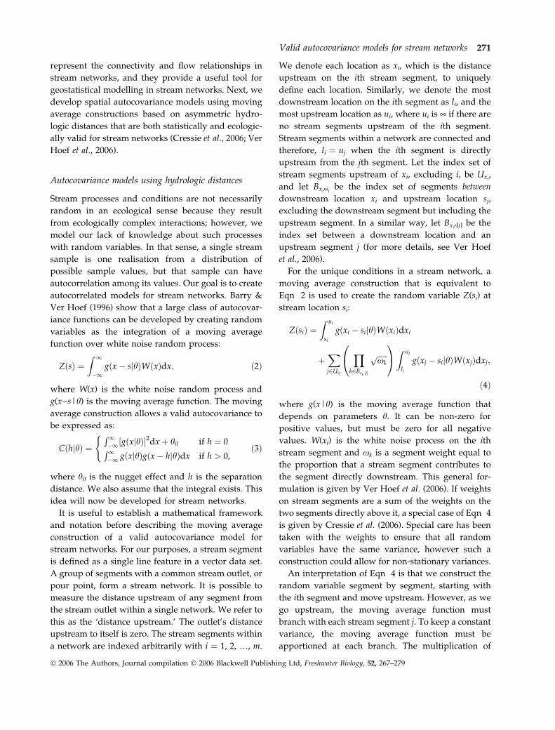
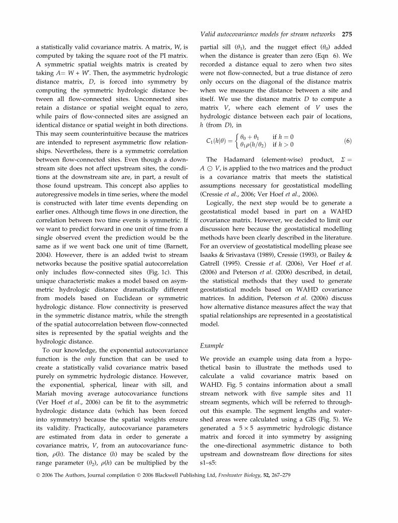
We provide an example using data from a hypo-

thetical basin to illustrate the methods used to

calculate a valid covariance matrix based on

WAHD. Fig. 5 contains information about a small

stream network with five sample sites and 11

stream segments, which will be referred to through-

out this example. The segment lengths and water-

shed areas were calculated using a GIS (Fig. 5). We

generated a 5 · 5 asymmetric hydrologic distance

matrix and forced it into symmetry by assigning

the one-directional asymmetric distance to both

upstream and downstream flow directions for sites

s1–s5:



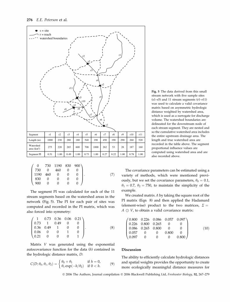
0 730 1190 830 900730 0 460 0 0

1190 460 0 0 0830 0 0 0 0900 0 0 0 0

0BBBB@

1CCCCA: ð7Þ

The segment PI was calculated for each of the 11

stream segments based on the watershed areas in the

network (Fig. 5). The PI for each pair of sites was

computed and recorded in the PI matrix, which was

also forced into symmetry:

1 0:73 0:36 0:06 0:210:73 1 0:49 0 00:36 0:49 1 0 00:06 0 0 1 00:21 0 0 0 1

0BBBB@

1CCCCA: ð8Þ

Matrix V was generated using the exponential

autocovariance function for the data (h) contained in

the hydrologic distance matrix, D:

CðD; h0; h1; h2Þ ¼h0 þ h1 if h ¼ 0,h1 expð�h=h2Þ if 0 < h.

ð9Þ

The covariance parameters can be estimated using a

variety of methods, which were mentioned previ-

ously, but we set the covariance parameters, h0 ¼ 0.1,

h1 ¼ 0.7, h2 ¼ 750, to maintain the simplicity of the

example.

We created matrix A by taking the square root of the

PI matrix (Eqn 8) and then applied the Hadamard

(element-wise) product to the two matrices, R ¼A x V, to obtain a valid covariance matrix:

0:800 0:226 0:086 0:057 0:0970:226 0:800 0:265 0 00:086 0:265 0:800 0 00:057 0 0 0:800 00:097 0 0 0 0:800

0BBBB@

1CCCCA ð10Þ

Discussion

The ability to efficiently calculate hydrologic distances

and spatial weights provides the opportunity to create

more ecologically meaningful distance measures for

1.000.781.000.220.271.000.731.000.491.000.51Segment PI

16018728532621000708600265220275Watershed area (km2)

5202602901904501905401802802301000Length (m)

r11r10r9r8r7r6r5r4r3r2r1Segment

s5

s = siter = reachwatershed boundaries

r3

r4

r5

r6

r7

s1

s2

s3

r1r2

r9 r8

s4

r10

r11Fig. 5 The data derived from this small

stream network with five sample sites

(s1–s5) and 11 stream segments (r1–r11)

was used to calculate a valid covariance

matrix based on asymmetric hydrologic

distance weighted by watershed area,

which is used as a surrogate for discharge

volume. The watershed boundaries are

delineated for the downstream node of

each stream segment. They are nested and

so the cumulative watershed area includes

the entire upstream drainage area. The

length and true watershed area are

recorded in the table above. The segment

proportional influence values are

computed using watershed area and are

also recorded above.



geostatistical modelling in stream networks. Until

recently, Euclidean distance has been the primary

distance measure used in geostatistical models. How-

ever, the physical characteristics of streams, such as

network configuration, connectivity, flow direction,

and position within the network, demand more

functional, process-based measures. Stream ecologists

will be able to choose models that are more appro-

priate for testing ecological hypotheses. In addition,

different patterns of spatial autocorrelation may occur

at coarse and fine scales, which could warrant model-

ling each pattern using a different distance measure.

Current models can be based on a variety of

distance measures, but it may also be possible to

create other more ecologically relevant distance meas-

ures that incorporate physical characteristics such as

flow velocity, stream gradient, or physical structures

that better reflect the energy an organism expends to

move from one location to another. Network connec-

tivity could also include chemical, physical and

biological barriers, such as pH, waterfalls and pred-

ators, to make the potential movement of organisms

and material more realistic. Given the complexity of

stream ecosystems, there is unlikely to be one meas-

ure of distance and connectivity that is most appro-

priate for all situations. Instead, providing a variety of

functional measures will facilitate exploration so that

stream ecologists can select or develop a measure

appropriate for their hypotheses.

As new functional distance measures are devel-

oped, it is imperative to be aware of the statistical

assumptions on which geostatistical models are

based. Stream ecologists and statisticians must ensure

that geostatistical models for stream networks are

both ecologically meaningful and statistically valid.

The tools and methodologies presented here pro-

vide an example of how to calculate the hydrologic

distances and spatial weights needed for geostatistical

modelling in stream networks. The tools described

here have been further developed as an ESRI ARCGISARCGIS

toolbox called the Functional Linkage of Watersheds

and Streams (FLoWS) (Theobald et al., 2005) and have

been made freely available to the public (http://

www.nrel.colostate.edu/projects/starmap/).

Acknowledgments

We thank Noel Cressie, Melinda Laituri, Brian Bledsoe,

Will Clements, and another anonymous reviewer for

their invaluable comments and suggestions; and the

U.S. Environmental Protection Agency for supporting

this work, which was developed under STAR Research

Assistance Agreement CR-829095 awarded to the

Space Time Aquatic Resource Modeling and Analysis

Program (STARMAP) at Colorado State University.

However, this paper has not been formally reviewed

by the EPA and the views expressed here are solely

those of the authors. Furthermore, the EPA does not

endorse any products mentioned in this paper.

References

Altunkaynak A., Ozger M. & Sen Z. (2003) Triple

diagram model of level fluctuations in Lake Van,

Turkey. Hydrology and Earth System Sciences, 7, 235–244.

Bailey T.C. & Gatrell A.C. (1995) Interactive Spatial Data

Analysis. Pearson Education Limited, Essex, U.K.

Barnett V. (2004) Environmental Statistics Methods and

Applications. John Wiley and Sons, Chichester, West

Sussex, U.K.

Barry R.P. & Ver Hoef J.M. (1996) Blackbox kriging:

spatial prediction without specifying the variogram.

Journal of Agricultural, Biological, and Environmental

Statistics, 1, 297–322.

Benda L., Poff N.L., Miller D., Dunne T., Reeves G., Pess

G. & Pollock M. (2004) The network dynamics

hypothesis: how channel networks structure riverine

habitats. BioScience, 54, 413–427.

Cressie N. (1993) Statistics for Spatial Data, Revised

edition. John Wiley and Sons, New York.

Cressie N., Frey J., Harch B. & Smith M. (2006) Spatial

prediction on a river network. Journal of Agricultural,

Biological, and Environmental Statistics, 11, 127–150.

Cumming G.S. (2002) Habitat shape, species invasions,

and reserve design: insights from simple models.

Conservation Ecology, 6, 3.

Dent C.L. & Grimm N.B. (1999) Spatial heterogeneity of

stream water nutrient concentrations over successional

time. Ecology, 80, 2283–2298.

Driscoll C.T., Lawrence G.B., Bulger A.J., Butler T.J.,

Cronan C.S., Eagar C., Lambert K.F., Likens G.E.,

Stoddard J.L. & Weathers K.C. (2001) Acid Rain

Revisited: Advances in Scientific Understanding since the

Passage of the 1970 and 1990 Clean Air Act Amendments.

Hubbard Brook Research Foundation, Hanover, NH.

Dussault G. & Brochu M. (2003) Distance Matrix Calcula-

tion. Institut Nationale de la Recherche Scientifique,

Urbanisation, Culture et Societe (INRS-UCS), Univer-

site du Quebec, Quebec, Canada. http://arcscripts.

esri.com (accessed 17 March 2005).



ESRI (2001) Hydro Data Model. Environmental Systems

Research Institute, Inc., Redlands, CA. http://suppor-

t.esri.com/index.cfm?fa¼downloads.dataModels.fil-

teredGateway&dmid¼15 (accessed 17 January 2005).

ESRI (2002) ArcGIS Version 8.3. Environmental Systems

Research Institute, Inc., Redlands, CA.

Fagan W.F. (2002) Connectivity, fragmentation, and

extinction risk in dendritic metapopulations. Ecology,

83, 3243–3249.

Fausch K.D., Torgersen C.E., Baxtor C.V. & Li H.W.

(2002) Landscapes to riverscapes: bridging the gap

between research and conservation of stream reaches.

Bioscience, 52, 483–498.

Ganio L.M., Torgersen C.E. & Gresswell R.E. (2005)

A geostatistical approach for describing spatial pattern

in stream networks. Frontiers in Ecology and the

Environment, 3, 138–144.

Gardner B., Sullivan P.J. & Lembo A.J. (2003) Predicting

stream temperatures: geostatistical model comparison

using alternative distance metrics. Canadian Journal of

Aquatic Science, 60, 344–351.

Handcock M. S. & Stein M. L. (1993) A Bayesian analysis

of kriging. Technometrics, 35, 403–410.

Herlihy A.T., Larsen D.P., Paulsen S.G., Urquhart N.S. &

Rosenbaum B.J. (2000) Designing a spatially balanced,

randomized site selection process for regional stream

surveys: The EMAP Mid-Atlantic Pilot Study. Environ-

mental Monitoring and Assessment, 63, 95–113.

Isaaks E.H. & Srivastava R.M. (1989) An Introduction to

Applied Geostatistics. Oxford University Press, Inc.,

New York.

Kellum B. (2002) Analysis and Modeling of Acid Neut-

ralizing Capacity in the Mid-Atlantic Highlands Area.

MS Thesis, Colorado State University, Fort Collins, CO,

69 pp.

Kneib R.T. (1994) Spatial pattern, spatial scale, and

feeding in fishes. In: Theory and Application in Fish

Feeding Ecology (Eds D.J. Strouder, K.L. Fresh & R.J.

Feller), pp. 170–185. Belle W. Baruch Library in Marine

Sciences, no. 18. University of South Carolina Press,

Columbia, SC.

Legleiter C.J., Lawrence R.L., Fonstad M.A., Marcus W.A.

& Aspinall R. (2003) Fluvial response a decade after

wildfire in the northern Yellowstone ecosystem: a

spatially explicit analysis. Geomorphology, 54, 119–136.

Little L.S., Edwards D. & Porter D.E. (1997) Kriging in

estuaries: as the crow flies, or as the fish swims?

Journal of Experimental Marine Biology and Ecology, 213,

1–11.

Mixon D.M. (2002) Automatic Watershed Location and

Characterization with GIS for an Analysis of Reservoir

Sediment Patterns. University of Colorado, Boulder, CO,

117 pp.

Neitsch S.L., Arnold J.G., Kiniry J.R., Srinivasan R. &

Williams J.R. (2002) Soil and Water Assessment Tool

User’s Manual. Texas Water Resources Institute, Col-

lege Station, TX.

Olden J.D., Jackson D.A. & Peres-Neto P.R. (2001) Spatial

isolation and fish communities in drainage lakes.

Oecologia, 127, 572–585.

Olea R.A. (1991) Geostatistical Glossary and Multilingual

Dictionary. Oxford University Press, New York.

Olsen A.R. & Ivanovich M. (1993) EMAP Monitoring

Strategy and Sampling Design. Video. U.S. Environmen-

tal Protection Agency, Office of Research and Devel-

opment, Environmental Research Laboratory,

Corvallis, OR.

Peterson E.E., Merton A.A., Theobald D.M. & Urquhart

N.S. (2006) Patterns of spatial autocorrelation in stream

water chemistry. Environmental Monitoring and Assess-

ment, 121, 615–638.

Pringle C.M. (2001) Hydrologic connectivity and the

management of biological reserves: a global perspec-

tive. Ecological Applications, 11, 981–998.

Rathbun S.L. (1998) Spatial modelling in irregularly

shaped regions: kriging estuaries. Environmetrics, 9,

109–129.

Theobald D.M. (2002) RW Tools for ArcView Version 3.

Unpublished program. Natural Resource Ecology

Laboratory, Fort Collins, CO.

Theobald D.M., Norman J., Peterson E.E. & Ferraz S.

(2005) Functional Linkage of Watersheds and Streams

(FLoWs): network-based ArcGIS tools to analyze freshwater

ecosystems. Proceedings of the ESRI User Conference 2005,

San Diego, CA, July 26.

Torgersen C.E., Gresswell R.E. & Bateman D.S. (2004)

Pattern detection in stream networks: quantifying

spatial variability in fish distribution. In: Proceedings

of the Second Annual International Symposium on GIS/

Spatial Analyses in Fishery and Aquatic Sciences (Eds

T. Nishida, P.J. Kailola & C.E. Hollingworth), pp. 405–

420. Fishery GIS Research Group, Saitama, Japan.

USEPA (2001) Survey Designs for Sampling Surface Water

Condition in the West. EPA A620/R-01/004c. USEPA

Office of Research and Development, Washington, DC.

USEPA (2002) NHD Reach Indexing Tool User’s Guide.

USEPA Office of Water, Washington, DC.

USGS (2004a) National Hydrography Dataset. U.S. Depart-

ment of the Interior, Rolla, MO. http://nhd.usgs.gov

(accessed 27 January 2005).

USGS (2004b) StreamStats. U.S. Department of the Inter-

ior, Washington, DC. http://streamstats.usgs.gov

(accessed 3 March 2005).

Ver Hoef J.M., Peterson E.E & Theobald D. (2006) Spatial

statistical models that use flow and stream distance.

Environmental and Ecological Statistics, 13, 449–464.



Ver Hoef J.M., Cressie N., Fisher R.N. & Case T.J. (2001)

Uncertainty and spatial linear models for ecological

data. In: Spatial Uncertainty for Ecology: Implications for

Remote Sensing and GIS Applications (Eds C.T. Hunsa-

ker, M.F. Goodchild, M.A. Friedl & T.J. Case), pp. 214–

237. Springer-Verlag, New York.

Vogel R.M., Wilson I. & Daly C. (1999) Regional

regression models of annual streamflow for the United

States. Journal of Irrigation and Drainage Engineering,

125, 148–157.

Ward J.V. (1989) The four-dimensional nature of lotic

ecosystems. Journal of the North American Benthological

Society, 8, 2–8.

Ward J.V., Tockner K., Arscott D.B. & Claret C. (2002)

Riverine landscape diversity. Freshwater Biology, 47,

517–539.

Wiens J.A. (2002) Riverine landscapes: taking landscape

ecology into the water. Freshwater Biology, 47, 501–515.

Yuan L.L. (2004) Using spatial interpolation to estimate

stressor levels in unsampled streams. Environmental

Monitoring and Assessment, 94, 23–38.

(Manuscript accepted 26 October 2006)



Geostatistical modelling on stream networks: developing valid ...

Documents

Transcript of Geostatistical modelling on stream networks: developing valid ...