Guia para a formatação de teses Versão 4.0 Janeiro 2006

GEOSPATIAL ASSESSMENT OF PEST-INDUCED FOREST DAMAGE THROUGH THE USE OF UAV-BASED NIR IMAGING AND GI-TECHNOLOGY

Oleksii Soloviov

ii

GEOSPATIAL ASSESSMENT OF PEST-INDUCED FOREST

DAMAGE THROUGH THE USE OF UAV-BASED

NIR IMAGING AND GI-TECHNOLOGY

Dissertation supervised by

Professor Mário Caetano, PhD

Instituto Superior de Estatística e Gestão de Informação

Universidade Nova de Lisboa

Lisbon, Portugal

Dissertation co-supervised by

Professor Torsten Prinz, PhD

Institut für Geoinformatik, Westfälische Wilhelms-Universität Münster

Münster, Germany

Dissertation co-supervised by

Professor Filiberto Pla, PhD

Departamento de Lenguajes y Sistemas Informatícos

Universitat Jaume I

Castellón, Spain

February 2014

iii

ACKNOWLEDGMENTS

First of all, I would like to thank Prof. Mário Caetano, because his valuable

advice and guidance helped me in writing my thesis project. I am very grateful to

Dr. Torsten Prinz for giving me an opportunity to work on this thesis, for his

explanations and criticism. Also, I am very thankful to Prof. Filiberto Pla for

remarks and useful comments in my research.

I would offer deep gratitude to Joel Dinis for his suggestions, patience and

good humor. He was happy to help in any possible way. Also, I want to thank

Christian Knoth (Institut für Geoinformatik), for advice and aid in vegetation indices

calculations.

I am grateful to Jan Lehmann (Institut für Landschaftsökologie), because he

was a pilot of UAV, and gave me some advices for image preprocessing.

Special thank for Christoph Hentschel (Wald und Holz NRW Soest – Sauerland

forest agency) for his help in providing necessary information about forest, getting

permissions to carry out flight campaign on private property and also providing

transport.

Thanks to all professors and universities staff for providing facilities and

excellent organization of Master of Geospatial Technologies Program. I am grateful

to my family and my friend Nikita Shumskych for their support and help.

Finally, I want to thank European Commission for giving me a chance to

participate in Master of Geospatial Technologies Program.

iv

GEOSPATIAL ASSESSMENT OF PEST-INDUCED FOREST

DAMAGE THROUGH THE USE OF UAV-BASED

NIR IMAGING AND GI-TECHNOLOGY

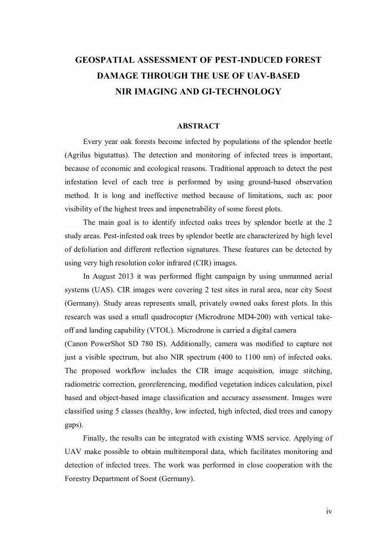
ABSTRACT

Every year oak forests become infected by populations of the splendor beetle

(Agrilus bigutattus). The detection and monitoring of infected trees is important,

because of economic and ecological reasons. Traditional approach to detect the pest

infestation level of each tree is performed by using ground-based observation

method. It is long and ineffective method because of limitations, such as: poor

visibility of the highest trees and impenetrability of some forest plots.

The main goal is to identify infected oaks trees by splendor beetle at the 2

study areas. Pest-infested oak trees by splendor beetle are characterized by high level

of defoliation and different reflection signatures. These features can be detected by

using very high resolution color infrared (CIR) images.

In August 2013 it was performed flight campaign by using unmanned aerial

systems (UAS). CIR images were covering 2 test sites in rural area, near city Soest

(Germany). Study areas represents small, privately owned oaks forest plots. In this

research was used a small quadrocopter (Microdrone MD4-200) with vertical take-

off and landing capability (VTOL). Microdrone is carried a digital camera

(Canon PowerShot SD 780 IS). Additionally, camera was modified to capture not

just a visible spectrum, but also NIR spectrum (400 to 1100 nm) of infected oaks.

The proposed workflow includes the CIR image acquisition, image stitching,

radiometric correction, georeferencing, modified vegetation indices calculation, pixel

based and object-based image classification and accuracy assessment. Images were

classified using 5 classes (healthy, low infected, high infected, died trees and canopy

gaps).

Finally, the results can be integrated with existing WMS service. Applying of

UAV make possible to obtain multitemporal data, which facilitates monitoring and

detection of infected trees. The work was performed in close cooperation with the

Forestry Department of Soest (Germany).

v

KEYWORDS

Color-infrared Images (CIR)

Near-infrared Images (NIR)

Object-based Classification

Pest Infestation

Pixel-based Classification

Principal Component

Unmanned Aerial Vehicle

Vegetation Indices

Very High Resolution Images

vi

ACRONYMS

AOI Study Area

CIR Color Infrared

EM spectrum Electromagnetic Spectrum

GCS Ground Control Station

GI-technology Geographic Information Technology

HALE High Altitude Long Endurance Vehicle

h_infected High Infected Trees

l_infected Low Infected Trees

MALE Medium Altitude Long Endurance vehicle

MTOW Maximum Take-Off Weight

MUAV Mini Unmanned Aerial Vehicle

NIR Near Infrared

UAS Unmanned Aerial Systems

UAV Unmanned Aerial Vehicle

VI Vegetation Indices

VTOL Vertical Take-Off And Landing

WMS Web Map Service

vii

TABLE OF CONTENTS

Page

ACKNOWLEDGEMENTS.........................................................................................iii

ABSTRACT................................................................................................................iv

KEYWORDS................................................................................................................v

ACRONYMS...............................................................................................................vi

INDEX OF TABLES...................................................................................................ix

INDEX OF FIGURES..................................................................................................x

INDEX OF FORMULAS…………………………………………………………...xii

1. INTRODUCTION…………………………………………………………………1

1.1 Background………………………………………………………...............1

1.2 Objective and Tasks………………………………………………………..3

2. LITERATURE REVIEW………………………………………………………….4

2.1 UAV in Forestry……………………………………………………………4

2.2 The Most Common Vegetation Indices. Classification…………………….5

2.3 Modified Vegetation Indices……………………………………………….8

3. DATASETS………………………………………………………………………10

3.1 Study Area and Geographic Context……………………………………...10

3.1.1 Climate……………...………………………………………….....12

3.1.2 Forest…………………………………….…………..………..…..13

3.2 Dataset………….…………………………………………………………14

3.2.1 UAV Imagery………….………………………………………….14

3.2.2 Ancillary Data…………………………….………………………16

4. METHODS……………………………………………………………………….20

4.1 UAV as Remote Sensing Platform………………………………………..20

4.2 UAV Color-infrared Imagery……………………………………………..24

4.3 Workflow………………………………………………………………….28

4.3.1 Pre-processing…………………………………………………….28

4.3.2 Classification……………………………………………………...33

4.3.2.1 Pixel based Classification………………………………...34

4.3.2.2 Object based Classification………………………………34

viii

4.3.3 Post-processing…………………………………………………...35

4.4 Accuracy Assessment……………………………………………………..35

5. RESULTS AND DISCUSSION………………………………………………….40

6. CONCLUSION…………………………………………………………………...54

BIBLIOGRAPHIC REFERENCES………………………………………………...55

APPENDIX …………………………………………………………………………60

ix

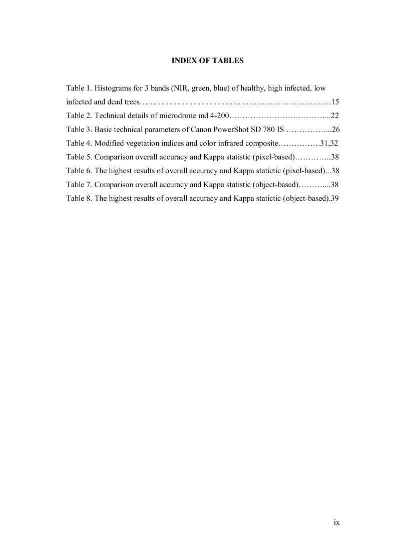
INDEX OF TABLES

Table 1. Histograms for 3 bands (NIR, green, blue) of healthy, high infected, low

infected and dead trees………………………………………………………………15

Table 2. Technical details of microdrone md 4-200………………………………...22

Table 3. Basic technical parameters of Canon PowerShot SD 780 IS ……………...26

Table 4. Modified vegetation indices and color infrared composite…………….31,32

Table 5. Comparison overall accuracy and Kappa statistic (pixel-based)…………..38

Table 6. The highest results of overall accuracy and Kappa statictic (pixel-based)...38

Table 7. Comparison overall accuracy and Kappa statistic (object-based)………....38

Table 8. The highest results of overall accuracy and Kappa statictic (object-based).39

x

INDEX OF FIGURES

Figure 1. Barely passable forest……………………………………………………....2

Figure 2. Location of study areas, Soest, Germany…………………………………10

Figure 3. Location of study area 1 and adjecent areas.…………………………...…11

Figure 4. Location of study area 2 and adjecent areas.…………………………...…11

Figure 5. Oak splendor beetle……………………………………………...………..13

Figure 6. Very high resolution color-infrared (CIR) aerial photograph ……..……..14

Figure 7. Adult and adjacent young oaks…………………...……………...………..16

Figure 8. GPS track of ground observation AOI 1………………………...………..17

Figure 9. GPS track of ground observation AOI 2………………………...………..17

Figure 10. GPS points of infected for AOI 1 (left) and AOI 2 (right)……………....18

Figure 11. Categories of UAS ……………………………………………………....20

Figure 12. Quadrocopter microdrone md 4-200………………………………...…..21

Figure 13. Rotor movement direction of quadrotor.…………………………...……23

Figure 14. Quadrotor dynamics.…………………………...……………………..…23

Figure 15. Digital image……....…………………………...……………………..…24

Figure 16. The EM spectrum and an idealized spectral reflectance curve of a healthy

vegetation.……………………………………………………………………….…..25

Figure 17. Digital compact camera Canon PowerShot SD 780 IS.………..……..…26

Figure 18. Example of reflectance of healthy and unhealthy trees………….............26

Figure 19. Filter configurations for natural color, NIR and CIR images....................27

Figure 20. Digital images in natural color, near infrared and the color infrared

composite………………………………………………………………....................28

Figure 21. Scheme of methodology……………………………………………........29

Figure 22. Cutting unsharp edges of images………………………………………...30

Figure 23. Image stitching…………………………………………………………..30

Figure 24. Boundary of ellipse plotted………………………………………….…..32

Figure 25. First principal component……………………………………….……….33

Figure 26. Second principal component……………………………………….……33

Figure 27. Example of test features in supervised classification…………………....34

Figure 28. Interpretation of Kappa..……………..…………………………………..36

xi

Figure 29. Control points………….....……………..……….……………………....37

Figure 30. Green NDVI. Modified Vegetation indices.………..…………................40

Figure 31. Blue NDVI. Modified vegetation indices.……………………………….41

Figure 32. GB NDVI. Modified vegetation indices.……..………………………….41

Figure 33. GSAVI. Modified vegetation indices.……..…………………………….41

Figure 34. Color-infrared composite…………………..…………………………….42

Figure 35. Principal component analysis……….……..…………………………….42

Figure 36. Pixel-based classification of Green NDVI………………………………43

Figure 37. Pixel-based classification of Blue NDVI………………………………..43

Figure 38. Pixel-based classification of GB NDVI…………………………………44

Figure 39. Pixel-based classification of GSAVI…………………………………….44

Figure 40. Pixel-based classification of color-infrared composite………………….45

Figure 41. Pixel-based classification of principal component analysis……………..45

Figure 42. Object-based classification of Green NDVI……………………………..46

Figure 43. Object-based classification of Blue NDVI………………………………46

Figure 44. Object-based classification of GB NDVI………………………………..47

Figure 45. Object-based classification of GSAVI…………………………………..47

Figure 46. Object-based classification of color-infrared composite………………...47

Figure 47. Object-based classification of principal component……………………..48

Figure 48. Results of manual correction of automatic delenition of GB NDVI.……48

Figure 49. Final map (1st study area)………………………………………………..49

Figure 50. All classes of 1st test site by area………………………………………...50

Figure 51. Final map (2nd study area)……………………………………………….51

Figure 52. All classes of 2nd test site by area………………………………………..52

xii

INDEX OF FORMULAS

Formula 1. NDVI (Normalized Difference Vegetation Index)………...…….……....6

Formula 2. Enhanced vegetation Index (EVI)……..………………...……………....6

Formula 3. Water Hand Index (WBI)……….……..………………...……………....6

Formula 4. Anthocyanin reflectance index (ARI_700)………………...…………....7

Formula 5. Kappa analysis………………...…………...............................................35

1

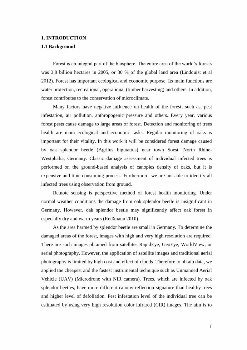
1. INTRODUCTION

1.1 Background

Forest is an integral part of the biosphere. The entire area of the world’s forests

was 3.8 billion hectares in 2005, or 30 % of the global land area (Lindquist et al

2012). Forest has important ecological and economic purpose. Its main functions are

water protection, recreational, operational (timber harvesting) and others. In addition,

forest contributes to the conservation of microclimate.

Many factors have negative influence on health of the forest, such as, pest

infestation, air pollution, anthropogenic pressure and others. Every year, various

forest pests cause damage to large areas of forest. Detection and monitoring of trees

health are main ecological and economic tasks. Regular monitoring of oaks is

important for their vitality. In this work it will be considered forest damage caused

by oak splendor beetle (Agrilus bigutattus) near town Soest, North Rhine-

Westphalia, Germany. Classic damage assessment of individual infected trees is

performed on the ground-based analysis of canopies density of oaks, but it is

expensive and time consuming process. Furthermore, we are not able to identify all

infected trees using observation from ground.

Remote sensing is perspective method of forest health monitoring. Under

normal weather conditions the damage from oak splendor beetle is insignificant in

Germany. However, oak splendor beetle may significantly affect oak forest in

especially dry and warm years (Reißmann 2010).

As the area harmed by splendor beetle are small in Germany. To determine the

damaged areas of the forest, images with high and very high resolution are required.

There are such images obtained from satellites RapidEye, GeoEye, WorldView, or

aerial photography. However, the application of satellite images and traditional aerial

photography is limited by high cost and effect of clouds. Therefore to obtain data, we

applied the cheapest and the fastest instrumental technique such as Unmanned Aerial

Vehicle (UAV) (Microdrone with NIR camera). Trees, which are infected by oak

splendor beetles, have more different canopy reflection signature than healthy trees

and higher level of defoliation. Pest infestation level of the individual tree can be

estimated by using very high resolution color infrared (CIR) images. The aim is to

2

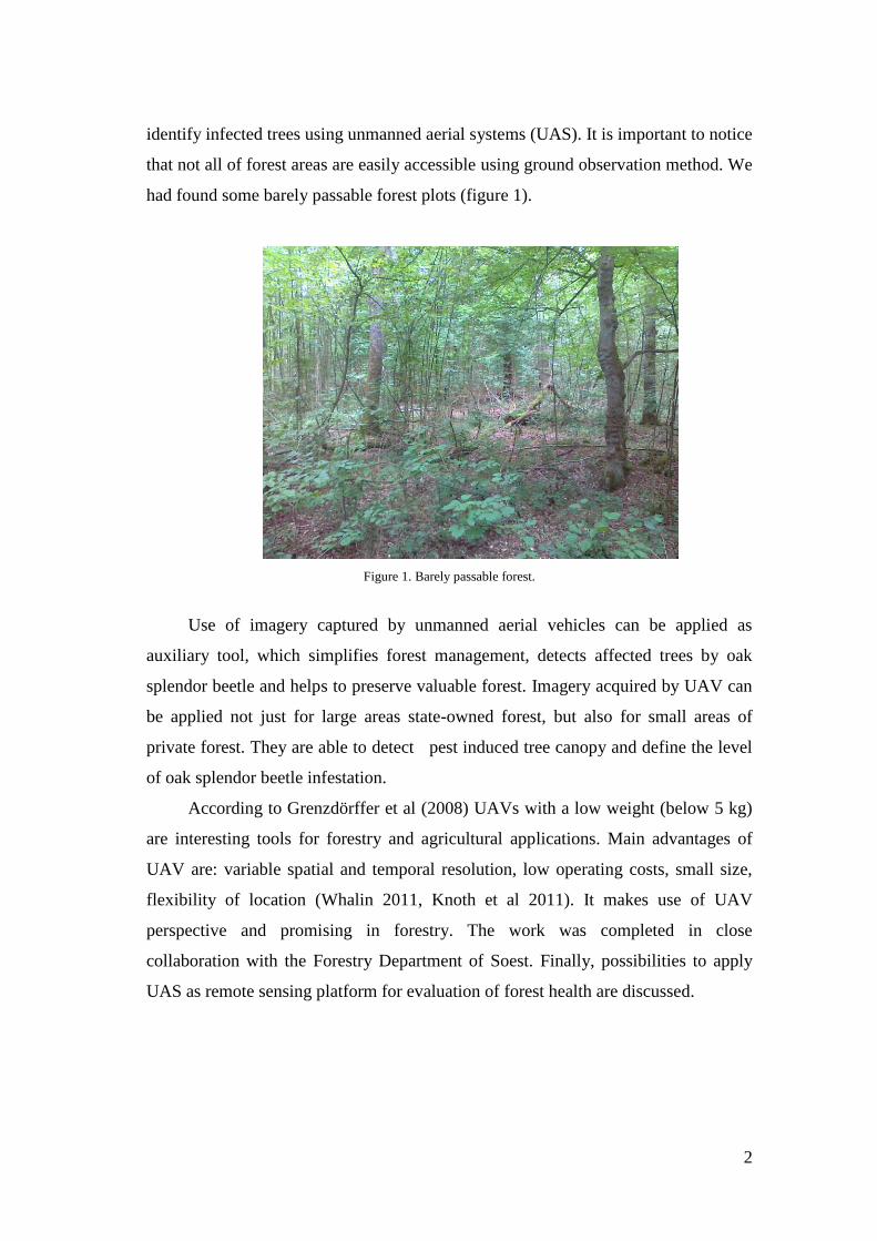
identify infected trees using unmanned aerial systems (UAS). It is important to notice

that not all of forest areas are easily accessible using ground observation method. We

had found some barely passable forest plots (figure 1).

Figure 1. Barely passable forest.

Use of imagery captured by unmanned aerial vehicles can be applied as

auxiliary tool, which simplifies forest management, detects affected trees by oak

splendor beetle and helps to preserve valuable forest. Imagery acquired by UAV can

be applied not just for large areas state-owned forest, but also for small areas of

private forest. They are able to detect pest induced tree canopy and define the level

of oak splendor beetle infestation.

According to Grenzdörffer et al (2008) UAVs with a low weight (below 5 kg)

are interesting tools for forestry and agricultural applications. Main advantages of

UAV are: variable spatial and temporal resolution, low operating costs, small size,

flexibility of location (Whalin 2011, Knoth et al 2011). It makes use of UAV

perspective and promising in forestry. The work was completed in close

collaboration with the Forestry Department of Soest. Finally, possibilities to apply

UAS as remote sensing platform for evaluation of forest health are discussed.

3

1.2 Objective and Tasks

The main research question is: “Is it possible to evaluate the level of pest

infestation of individual oak’s trees by using UAV NIR very high resolution images

in order to obtain new geospatial data for forest health management ?”

The main goal is to define the level of infestation oaks trees by Splendor beetle

infection at the study areas.

The main tasks in this work are:

- using UAV based imagery to obtain recent geo-data of infected oaks by oaks

splendor beetle;

- GIS-analysis of the accumulated data (UAV, GPS data, WMS);

- to specify level of infections of the trees;

- to identify the best modified vegetation indices for detection of infected trees;

- to compare pixel based and object based classification method.

4

2. LITERATURE REVIEW

2.1 UAV in Forestry

First efforts to represent aerial photographs as a tool of remote sensing were

made in 1887. The forest was classified and characterized, basing on visual

inspection of photographs. Research of storm damage, using aerial photographs,

were, perhaps, the first application for forest health using remote sensing. Aerial

photography has been widely practiced for civil use after World War 2. Since then

aerial images were used for forestry application. Forest inventory and measurements

are the most widely used applications of aerial imagery (Tuominen et al 2009).

In recent years the technological process of acquiring remote sensing data has

developed rapidly. Use of UAVs is faster, safer, and cheaper than airborne

photography. UAVs are able to obtain very high resolution imagery. These

advantages make UAVs ideal for use in forest applications. UAV imagery offers the

ability to detect and map spatial characteristics of vegetation and gaps between

vegetation patches associated with erosion risk (Albert 2009).

The application of UAV in forest monitoring purposes is particularly effective

for small and medium areas. For example, UAVs can be used for:

• Forestry and nature conservation.

• Forest fire detection. Frequent updates regarding the progress of a forest fire

are necessary for effective firefighting. Small unmanned aerial vehicles (UAVs) are

emerging as promising tools for forest fires monitoring (David et al 2005).

• Timber Theft. Challenges include extensive forest boundaries, hardship in

finding the boundary on the ground, and the lack of manpower to actually monitor

for illegal logging. UAVs can be programmed to fly round the boundaries of large

forest holdings. Any illegal forest activity can be identified using UAV imagery.

• Road Maintenance. Forest roads are usually the main source of erosion in

forest operations. Even closed roads and trails are problems. Use of the UAVs ability

to display the corridor can be also programmed. For example, it can fly over the

complete road network of forest and check the drainage facilities (Horcher et al

2004).

• Segmentation of tree crowns (Hung et al 2012).

5

• Texture analysis. Texture is considered as a quantitative characteristic of the

image (Laliberte et al 2009, EM 2014).

• Remote chemistry is a new approach that permitted to access forest health

through identifying chemical composition of foliage (Tuominen et al 2009).

• Airborne Light Detection and Range (laser). This is becoming an increasingly

important tool for scientific research forest structure. Multi-temporal study using

laser scanning data showed also a capacity to assess forest dynamics, such as

changes in biomass, the gap fractions (Wallace 2012).

• UAVs can also be used for: biosecurity and disease monitoring; windfall

score, score planting density, site planning, monitoring of vegetation. UAV provides

monitoring and analysis of changes in natural forests, where disturbance is difficult

or undesirable (Horcher et al 2004, Zmarz 2009).

2.2 The most common vegetation indices. Classification

To access sensing of forest health using remote sensing technique it is

important to have high resolution aerial or satellite imagery of forest areas. In recent

years, technological process of remote sensing advanced rapidly. UAV application in

forest monitoring especially is useful for small and medium-sized forest areas. Based

on the amount of bands and wavelengths, images obtained by remote sensing can be

divided into aerial photography, multispectral and hyperspectral reflections. To

evaluate forest health using remote sensing methods, typically, vegetation indices are

extracted from images. They are decreasing the effects of irradiance and exposure

and increasing contrast between different features on image (Raymond et al 2008).

Vegetation indices are combinations of surface reflectance of two or more

wavelength. They highlight a specific property of vegetation. Vegetation indices

simplify detection of forest damage level (Tuominen et al 2009).

Calculation of vegetation indices, generally, uses red, green, blue and NIR

bands. Since information is contained in a single spectral band, it is usually

insufficient to characterize the vegetation status.

6

NDVI (Normalized Difference Vegetation Index) is one of the most known

vegetation indices. It measures the general quantity and vigor of green vegetation

(Tuominen et al 2009). NDVI is a function, which calculations are based on

reflectance of near infrared (NIR) and red bands. It is defined according to the

equation 1:

(1)

where NIR is near infrared band, RED is red band.

Enhanced vegetation Index (EVI) is developed to estimate dense of vegetation

areas. NDVI is excessively saturated at the dense vegetated areas. To solve this

problem the blue reflectance is used to compensate influence of background soil

effects and atmospheric scattering effects. EVI can be expressed in the following

equation 2:

(2)

where NIR is near infrared band, RED is red band, BLUE is blue band.

Water content in the leaves is significant vegetation property which correlates

with forest health.

The Water Hand Index (WBI) is an index that measures reflectance. It is

sensitive to changes in canopy water content. Water absorption feature at 970 nm is

utilized by Water Hand Index. The ratio of the reflectance is measured. Water Hand

Index 1 is determined in accordance with the equation 3:

(3)

where is reflectance.

7

The next index that measures the amount of stress-related pigments in

vegetation called Leaf Pigment Vegetation Index. Anthocyanins and carotenoids are

pigments which are detected in higher concentrations in the unhealthy vegetation.

Anthocyanin reflectance index (ARI_700) is sensitive to the anthocyanin amount in

leaves. Anthocyanin reflectance index is defined as provided by equation 4

(4)

where is reflectance (Tuominen et al 2009).

After calculation of vegetation indices it is necessary to perform classification

of data. Classification is grouping of existing object types in an image data.

Classification often uses remote sensing method for detecting and monitoring of the

environment. The first step in classification procedure is to define the number of

classes. Each pixel should be assigned as a class label. The second step is to select

classification method. There are two classification methods: pixel-based and object

based classification. Pixel-based classification assigns a class value to every pixel of

image. Classifications can be completed using object based method. Classification

divides images into homogeneous regions and then assigns the classes to each

segment. Classification process can be performed as supervised and unsupervised

classification. Unsupervised classification is executing automatically, following

selected algorithms (K-means and other.) Supervised classification is requesting user

to select training areas for each class. Supervised classification includes a learning

process through selecting training set. For an effective and accurate classification, the

training set should be selected from the same image. In the supervised classification

the spectral values are the basic statistical properties, which extracted from training

set. Each pixel’s (region’s class) is defined using similarity measure for individual

pixel spectral signatures and training set statistics (Duzgun et al 2011).

Pixel-based classification is a technique to extract “thematic classes” from

multi bands images. The most important limitation of pixel-based classification is

8

each pixel is assigned only one class. Spectral class is a class that connected to the

spectral band used in the classification. Spectral classes correspond to land cover

classes. Problem with pixel based classification is occurring when we have a few

classes per cell. In this case, pixel can be assigned to another class. This problem

usually named as the mixed pixel. Assigning the pixel to more than one class can be

solution of this problem.

Object oriented classification is divided an image into homogenous spectral

segments which correspond to buildings, forest, roads, etc. Each element is

homogenous by following characteristics: spectral appearance, shape, color,

compactness, texture and etc. (Wim et l 2009).

Generally, object-oriented classification is more effective than pixel-based one.

Object-oriented classification is closer to the manual interpretation, than pixel based

method. The size of objects can be quantified (OOC 2014). Due to impossibility to

calculate the most common vegetation indices, the modified vegetation indices were

calculated.

2.3 Modified vegetation indices

If one takes into account that the most common forest studies work with data

which contains several spectral bands (at least 4), in this study it is available an

imagery that has just 3 bands (NIR, green and blue). Consequently, we are not able

to calculate the most of vegetation indices, because most of them are required red

band. However, it is possible to calculate modified vegetation indices, where instead

of red band we use green and blue bands. Modified NDVI and SAVI indices would

be calculated. Green and blue bands also contain vegetation information. One of the

main tasks is to determine the best Vegetation Indices for detection of trees infected

by oak splendor beetle (Wang et al 2007). Instead of true color composite the color

infrared composite is applied.

According to (Wang et al 2007) the green channel of NDVI, it has a good

correlation with photosynthetic activity of vegetation. Sensitivity of visible

reflectance to chlorophyll shows that the green channel is more sensitive to

9

chlorophyll than the red one. Therefore, GNDVI was developed. The green channel

can be used to estimate the vegetation cover. The blue band also contains vegetation

information. It has been applied rarely in remote sensing for vegetation monitoring

(Wang et al 2007).

10

3. DATASETS

3.1 Study Area and Geographic Context

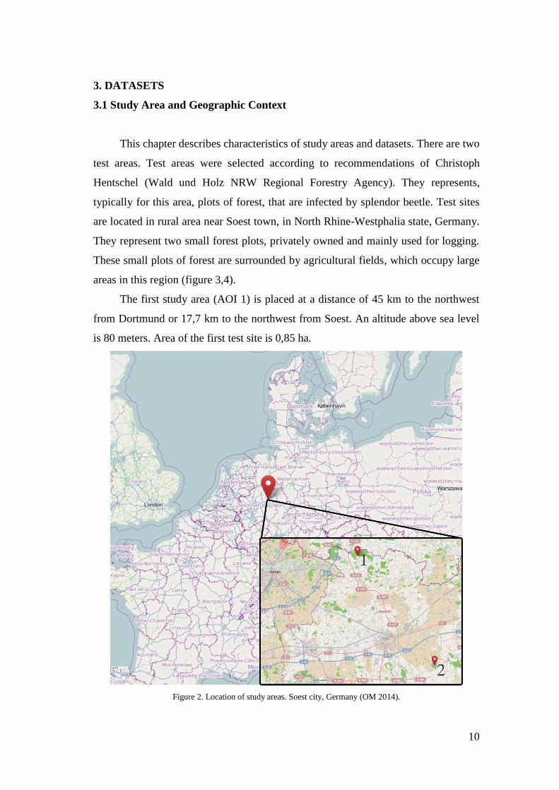
This chapter describes characteristics of study areas and datasets. There are two

test areas. Test areas were selected according to recommendations of Christoph

Hentschel (Wald und Holz NRW Regional Forestry Agency). They represents,

typically for this area, plots of forest, that are infected by splendor beetle. Test sites

are located in rural area near Soest town, in North Rhine-Westphalia state, Germany.

They represent two small forest plots, privately owned and mainly used for logging.

These small plots of forest are surrounded by agricultural fields, which occupy large

areas in this region (figure 3,4).

The first study area (AOI 1) is placed at a distance of 45 km to the northwest

from Dortmund or 17,7 km to the northwest from Soest. An altitude above sea level

is 80 meters. Area of the first test site is 0,85 ha.

Figure 2. Location of study areas. Soest city, Germany (OM 2014).

11

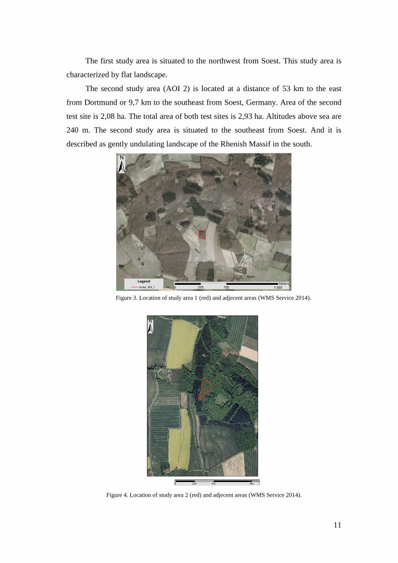
The first study area is situated to the northwest from Soest. This study area is

characterized by flat landscape.

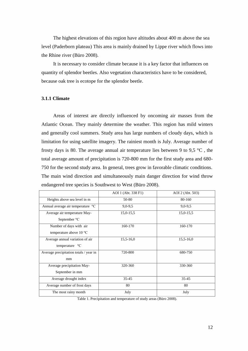
The second study area (AOI 2) is located at a distance of 53 km to the east

from Dortmund or 9,7 km to the southeast from Soest, Germany. Area of the second

test site is 2,08 ha. The total area of both test sites is 2,93 ha. Altitudes above sea are

240 m. The second study area is situated to the southeast from Soest. And it is

described as gently undulating landscape of the Rhenish Massif in the south.

Figure 3. Location of study area 1 (red) and adjecent areas (WMS Service 2014).

Figure 4. Location of study area 2 (red) and adjecent areas (WMS Service 2014).

12

The highest elevations of this region have altitudes about 400 m above the sea

level (Paderborn plateau) This area is mainly drained by Lippe river which flows into

the Rhine river (Büro 2008).

It is necessary to consider climate because it is a key factor that influences on

quantity of splendor beetles. Also vegetation characteristics have to be considered,

because oak tree is ecotope for the splendor beetle.

3.1.1 Climate

Areas of interest are directly influenced by oncoming air masses from the

Atlantic Ocean. They mainly determine the weather. This region has mild winters

and generally cool summers. Study area has large numbers of cloudy days, which is

limitation for using satellite imagery. The rainiest month is July. Average number of

frosty days is 80. The average annual air temperature lies between 9 to 9,5 °C , the

total average amount of precipitation is 720-800 mm for the first study area and 680-

750 for the second study area. In general, trees grow in favorable climatic conditions.

The main wind direction and simultaneously main danger direction for wind throw

endangered tree species is Southwest to West (Büro 2008).

AOI 1 (Abt. 338 F1) AOI 2 (Abt. 503)

Heights above sea level in m 50-80 80-160

Annual average air temperature °С 9,0-9,5 9,0-9,5

Average air temperature May-

September °С

15,0-15,5 15,0-15,5

Number of days with air

temperature above 10 °С

160-170 160-170

Average annual variation of air

temperature °С

15,5-16,0 15,5-16,0

Average precipitation totals / year in

mm

720-800 680-750

Average precipitation May-

September in mm

320-360 330-360

Average drought index 35-45 35-45

Average number of frost days 80 80

The most rainy month July July

Table 1. Precipitation and temperature of study areas (Büro 2008).

13

3.1.2 Forest

In the first test site English oak (Quercus robur) of 117 years old grows, as the

primary plant species. English oak is high quality wood (2nd

quality class by forestry

level classification). This test site is characterized by planar relief. Hornbeam

(Carpinus (betulus)) grows during 69 years, as secondary plant species. Also in this

area other tree species such as birch (Betula), common maple (Acer campestre) could

be found.

In the second test site English oak of 103 years old grows, as the primary plant

species. In the second test site English oak of 103 years old grows, as the primary

plant species. English oak belongs to middle quality wood (3rd

quality class by

forestry level classification). European beech (Fagus silvatica) is 48 years old (3rd

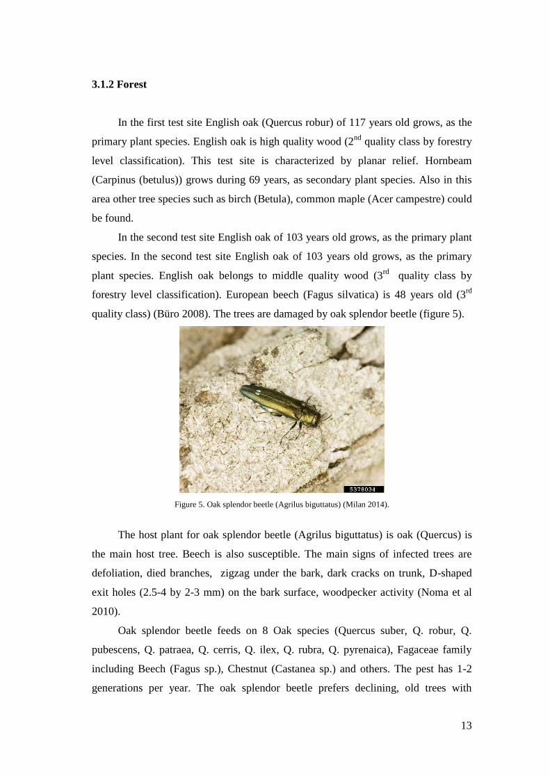
quality class) (Büro 2008). The trees are damaged by oak splendor beetle (figure 5).

Figure 5. Oak splendor beetle (Agrilus biguttatus) (Milan 2014).

The host plant for oak splendor beetle (Agrilus biguttatus) is oak (Quercus) is

the main host tree. Beech is also susceptible. The main signs of infected trees are

defoliation, died branches, zigzag under the bark, dark cracks on trunk, D-shaped

exit holes (2.5-4 by 2-3 mm) on the bark surface, woodpecker activity (Noma et al

2010).

Oak splendor beetle feeds on 8 Oak species (Quercus suber, Q. robur, Q.

pubescens, Q. patraea, Q. cerris, Q. ilex, Q. rubra, Q. pyrenaica), Fagaceae family

including Beech (Fagus sp.), Chestnut (Castanea sp.) and others. The pest has 1-2

generations per year. The oak splendor beetle prefers declining, old trees with

14

diameter about 30 cm. From May to the end of August adults can be observed. They

feed on foliage in the three canopies. Eggs usually hatch after 1 or 2 weeks. The

larvae bore through logs and easily can be found under the bark by zig-zag galleries.

(DOA 2014).

3.2 Dataset

3.2.1 UAV imagery

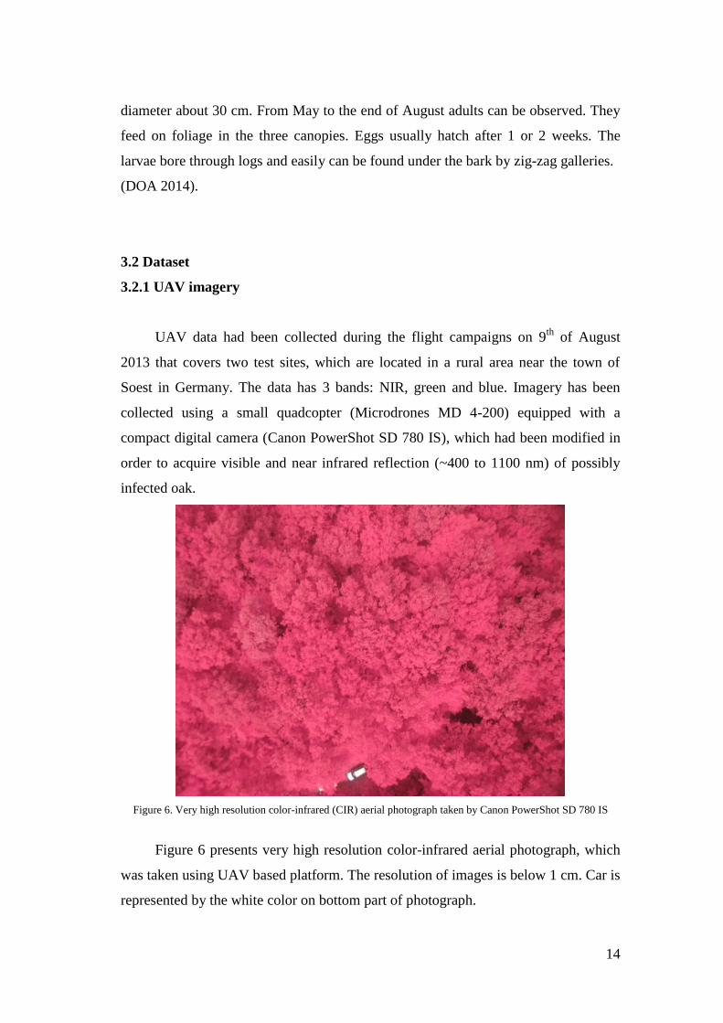
UAV data had been collected during the flight campaigns on 9th

of August

2013 that covers two test sites, which are located in a rural area near the town of

Soest in Germany. The data has 3 bands: NIR, green and blue. Imagery has been

collected using a small quadcopter (Microdrones MD 4-200) equipped with a

compact digital camera (Canon PowerShot SD 780 IS), which had been modified in

order to acquire visible and near infrared reflection (~400 to 1100 nm) of possibly

infected oak.

Figure 6. Very high resolution color-infrared (CIR) aerial photograph taken by Canon PowerShot SD 780 IS

Figure 6 presents very high resolution color-infrared aerial photograph, which

was taken using UAV based platform. The resolution of images is below 1 cm. Car is

represented by the white color on bottom part of photograph.

15

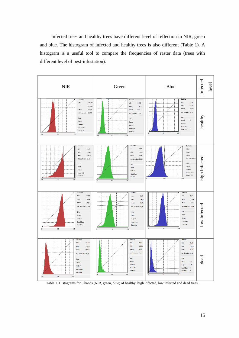
Infected trees and healthy trees have different level of reflection in NIR, green

and blue. The histogram of infected and healthy trees is also different (Table 1). A

histogram is a useful tool to compare the frequencies of raster data (trees with

different level of pest-infestation).

NIR

Green

Blue

Infe

cted

level

hea

lthy

hig

h i

nfe

cted

low

in

fect

ed

dea

d

Table 1. Histograms for 3 bands (NIR, green, blue) of healthy, high infected, low infected and dead trees.

16

The flight height of UAV is 68,5 m for first study area. The resolution is

0,62 (cm)/pixel (AOI 1). The flight height is 76 m for second study area (AOI 2).

The resolution is 0,69 (cm)/pixel (AOI 2). The spatial resolution was calculated by

author. The total number of acquired images is 116. All data is saved in JPG format.

3.2.2 Ancillary data

To detect the infected oaks, forest agency has applied a method of visual trees

observation from the ground. This method is several hundred years old. Forest

agency collects GPS points of low infected, high infected and died trees. Died and

high infected trees (trees with less than 30 % of leaves) are marked with special paint

symbol. It is necessary to cut high infected trees due to economic and ecological

reasons. If we do not cut infected trees in time, cracks begin to appear on the trunk of

trees. Such wood becomes ineligible for woodworking industry.

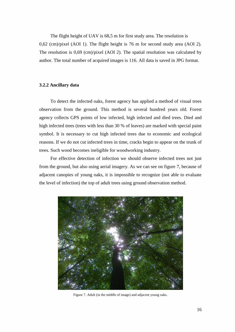
For effective detection of infection we should observe infected trees not just

from the ground, but also using aerial imagery. As we can see on figure 7, because of

adjacent canopies of young oaks, it is impossible to recognize (not able to evaluate

the level of infection) the top of adult trees using ground observation method.

Figure 7. Adult (in the middle of image) and adjacent young oaks.

17

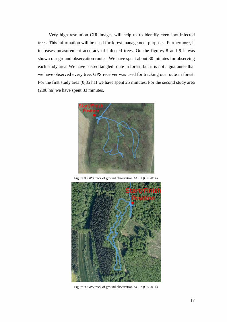
Very high resolution CIR images will help us to identify even low infected

trees. This information will be used for forest management purposes. Furthermore, it

increases measurement accuracy of infected trees. On the figures 8 and 9 it was

shown our ground observation routes. We have spent about 30 minutes for observing

each study area. We have passed tangled route in forest, but it is not a guarantee that

we have observed every tree. GPS receiver was used for tracking our route in forest.

For the first study area (0,85 ha) we have spent 25 minutes. For the second study area

(2,08 ha) we have spent 33 minutes.

Figure 8. GPS track of ground observation AOI 1 (GE 2014).

Figure 9. GPS track of ground observation AOI 2 (GE 2014).

18

Oak splendor beetle prefers warm condition; we can find this pest on the top of

trees. Canopy reflection of infected trees is different from health trees. In addition,

the level of defoliation indicates the level of pest infection. If we detect infected tree

in earlier level of infection, the forest agency can provide intensified monitoring of

this trees. In case, if infected tree has less than 30 % of leaves, it is necessary to cut

this tree. It is dangerous to cut too much trees in the forest, because in this way we

are changing microclimate (it is getting warmer in whole forest). If weather becomes

warmer, the number of oak splendor beetle increases, because this pest prefers warm

weather condition (DOA 2014).

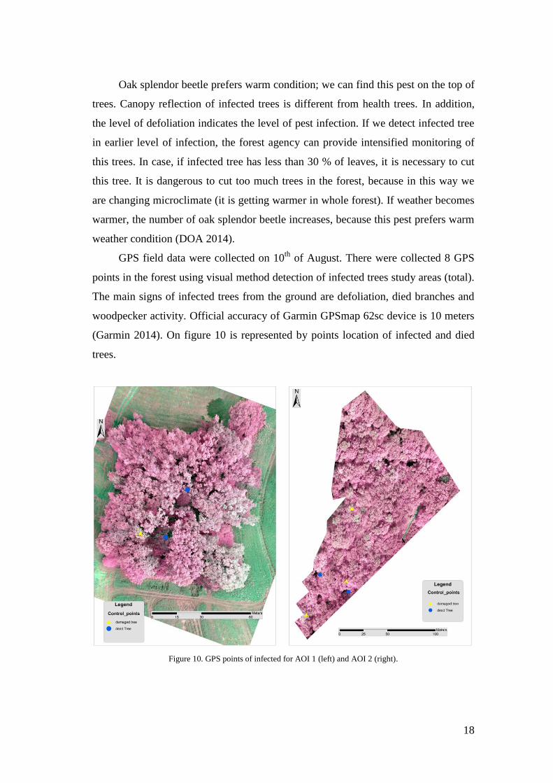
GPS field data were collected on 10th

of August. There were collected 8 GPS

points in the forest using visual method detection of infected trees study areas (total).

The main signs of infected trees from the ground are defoliation, died branches and

woodpecker activity. Official accuracy of Garmin GPSmap 62sc device is 10 meters

(Garmin 2014). On figure 10 is represented by points location of infected and died

trees.

Figure 10. GPS points of infected for AOI 1 (left) and AOI 2 (right).

19

Using ground observation method, 4 dead, 3 high infected and 1 low infected

trees in two test sites were detected. Garmin GPSmap 62sc device was used to track

route in forest and collection of points. It is important to notice that Soest forest

agency has its own 40 cm resolution orthophotography (WMS) of forest areas.

Existing orthophotography allows us to identify some large homogeneous plots of

died trees.

20

4. METHODS

4.1 UAV as remote sensing platform

This chapter describes the workflow of this thesis. Geographic information

technology is regarded as a set of GIS, remote sensing and visual interpretation

methods. We have used unmanned aerial vehicle (quadrocopter), as a remote sensing

platform for acquiring aerial photographs. The basic characteristics of quadrocopter

and optical camera were described. In this section we have overviewed the traditional

approach for detection of pest infected trees in forest. Quadrocopter was considered

as justified tool for data collection and promising tool for forestry management

purposes.

UAS has to be considered as a system, which consists of three different

components: 1) ground control station (GCS), via which the quadrocopter is

controlled. 2) Communication infrastructure component is providing connection

signal between the transmitter and the receiver (UAV); 3) aerial platform

(quadrocopter). The terms UAS and UAV usually are used as synonyms, but UAV

means the aerial platform only. UAS means all systems, which includes all three

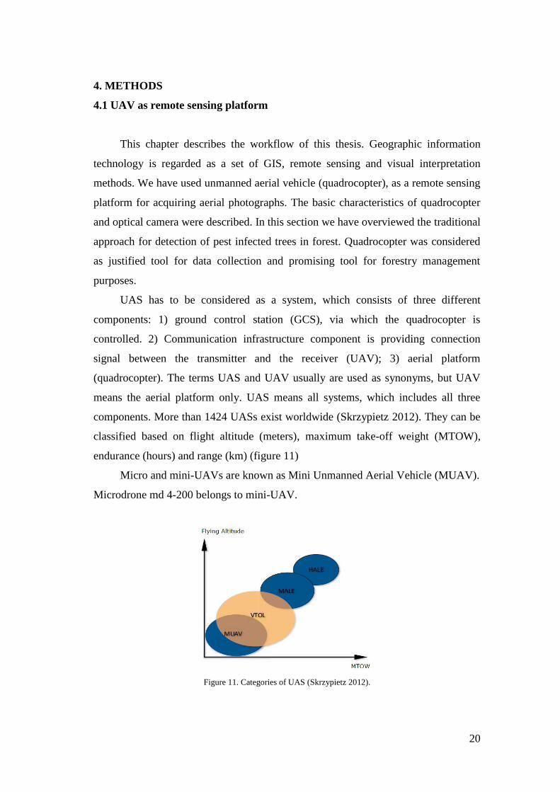
components. More than 1424 UASs exist worldwide (Skrzypietz 2012). They can be

classified based on flight altitude (meters), maximum take-off weight (MTOW),

endurance (hours) and range (km) (figure 11)

Micro and mini-UAVs are known as Mini Unmanned Aerial Vehicle (MUAV).

Microdrone md 4-200 belongs to mini-UAV.

Figure 11. Categories of UAS (Skrzypietz 2012).

21

Medium Altitude Long Endurance (MALE) and High Altitude Long

Endurance (HALE) are more complex and larger systems than MUAVs. They can

carry more payload and they can cover longer distances, comparing to mini-UAV

(Skrzypietz 2012).

Advantages and disadvantages of unmanned aerial vehicle method of data

collection and traditional approach were considered in this work. In the forestry,

relief is often a main hamper of application of UAS (planes) due to limited space for

take-off and landing. Copters with vertical take-off and landing (VTOL) capabilities

are a promising tool for forest management purposes (Soloviov et al 2014).

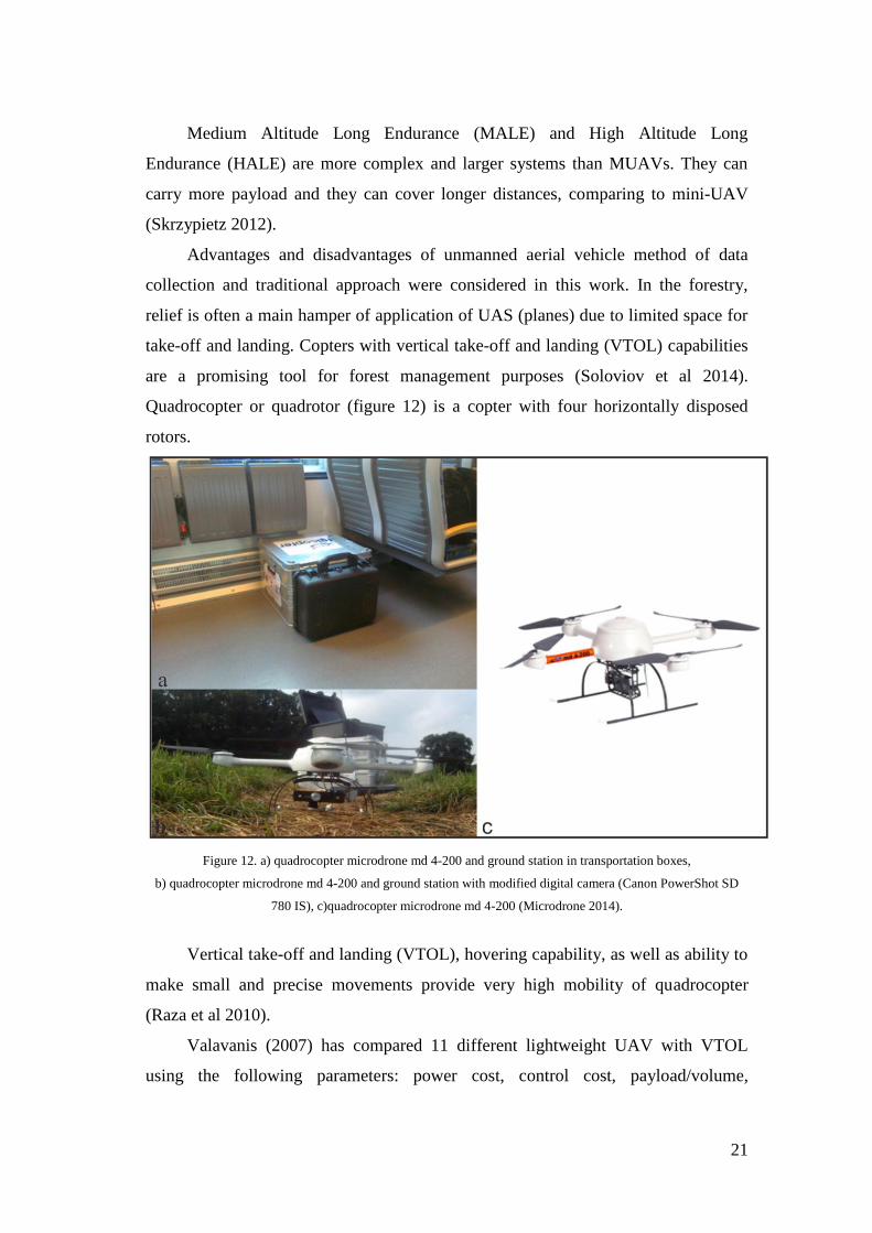
Quadrocopter or quadrotor (figure 12) is a copter with four horizontally disposed

rotors.

Figure 12. a) quadrocopter microdrone md 4-200 and ground station in transportation boxes,

b) quadrocopter microdrone md 4-200 and ground station with modified digital camera (Canon PowerShot SD

780 IS), c)quadrocopter microdrone md 4-200 (Microdrone 2014).

Vertical take-off and landing (VTOL), hovering capability, as well as ability to

make small and precise movements provide very high mobility of quadrocopter

(Raza et al 2010).

Valavanis (2007) has compared 11 different lightweight UAV with VTOL

using the following parameters: power cost, control cost, payload/volume,

22

maneuverability, mechanics simplicity, aerodynamics, complexity, low speed flight,

high-speed flight, miniaturization, survivability and stationary flight. Quadrocopter

(quadrotor) has the highest total evaluation rate. The microdrone MD 4-200 is

produced in Germany by company “Microdrone GmbH”. Some technical parameters

of microdrone MD4-200 are shown in the table 2.

Description Microdrones light quadrocopter

Technical specifications

Vehicle mass 800 g

Payload mass (recommended) 150 g

Payload mass (maximum) 250 g

Maximum take-off weight 1100g

Battery 4S LiPo, 14.8V, 2300 mAh

Climb rate 7 m/s

Cruising speed 8 m/s

Endurance Up to 30 minutes

Flight radius Up to 6000m

Operational condition’s

Wind tolerance Steady pictures up to 4 m/s

Dimensions

Diameter 540 mm

Height 230 mm

Table 2. Technical details of microdrone md 4-200 (Microdrone 2014)

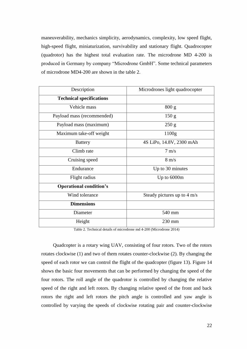
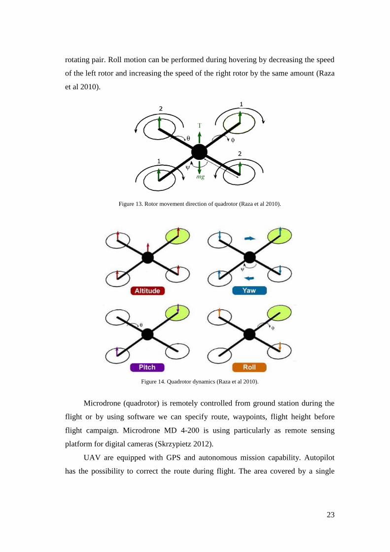
Quadcopter is a rotary wing UAV, consisting of four rotors. Two of the rotors

rotates clockwise (1) and two of them rotates counter-clockwise (2). By changing the

speed of each rotor we can control the flight of the quadcopter (figure 13). Figure 14

shows the basic four movements that can be performed by changing the speed of the

four rotors. The roll angle of the quadrotor is controlled by changing the relative

speed of the right and left rotors. By changing relative speed of the front and back

rotors the right and left rotors the pitch angle is controlled and yaw angle is

controlled by varying the speeds of clockwise rotating pair and counter-clockwise

23

rotating pair. Roll motion can be performed during hovering by decreasing the speed

of the left rotor and increasing the speed of the right rotor by the same amount (Raza

et al 2010).

Figure 13. Rotor movement direction of quadrotor (Raza et al 2010).

Figure 14. Quadrotor dynamics (Raza et al 2010).

Microdrone (quadrotor) is remotely controlled from ground station during the

flight or by using software we can specify route, waypoints, flight height before

flight campaign. Microdrone MD 4-200 is using particularly as remote sensing

platform for digital cameras (Skrzypietz 2012).

UAV are equipped with GPS and autonomous mission capability. Autopilot

has the possibility to correct the route during flight. The area covered by a single

24

flight may cover several square kilometers with an operational flight time of 30-40

minutes (Zmarz 2009).

In this work was used a small quadrotor UAS (Microdrones MD 4-200)

equipped with a compact digital camera (Canon PowerShot SD 780 IS). The flight

campaigns were performed in August 2013 covering two test sites which are located

in a rural area near the town of Soest in Germany (Soloviov et al 2014).

UAV image acquisition has certain limitations. They refer to performing flight

campaign. Flight campaign was delayed for almost 2 weeks due to unsuitable

weather condition: strong wind, rain and cloudy sky.

4.2 UAV color-infrared imagery

For detailed consideration of UAV color-infrared imagery it is necessary to

understand general principles of remote sensing. Electromagnetic (EM) spectrum is

total range of wavelengths of EM radiation. Top part of figure 16 illustrates the total

spectrum of EM radiation. Each of the part of EM spectrum represents not one

particular wavelength, but a range of wavelength (Wim et al 2009). An image is two-

dimensional way of representation features in a real scene. Images represent the parts

of the earth surface from space. There are 2 types of images: analog and digital. A

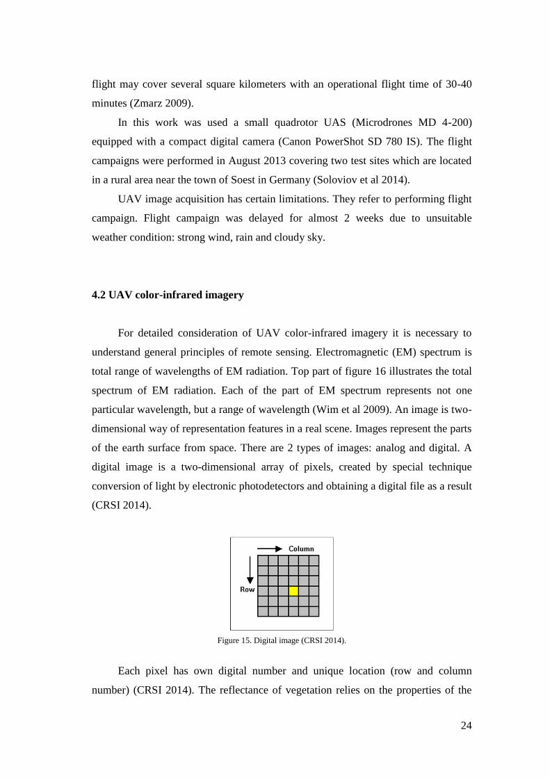
digital image is a two-dimensional array of pixels, created by special technique

conversion of light by electronic photodetectors and obtaining a digital file as a result

(CRSI 2014).

Figure 15. Digital image (CRSI 2014).

Each pixel has own digital number and unique location (row and column

number) (CRSI 2014). The reflectance of vegetation relies on the properties of the

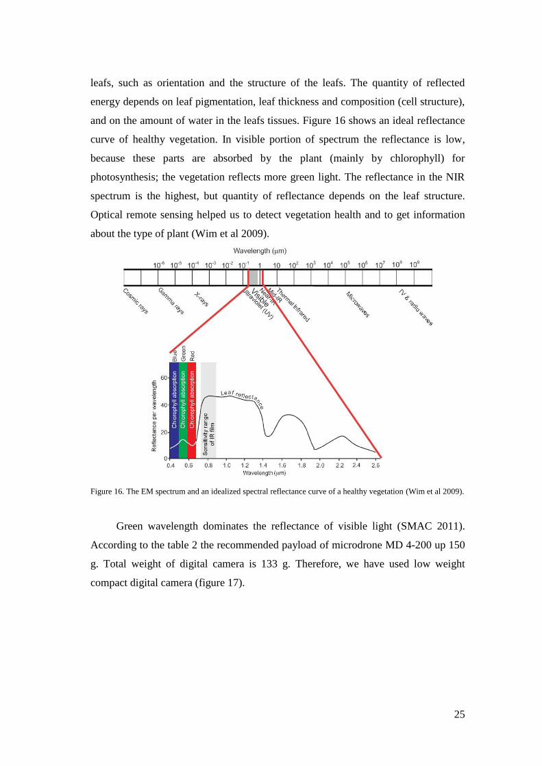
25

leafs, such as orientation and the structure of the leafs. The quantity of reflected

energy depends on leaf pigmentation, leaf thickness and composition (cell structure),

and on the amount of water in the leafs tissues. Figure 16 shows an ideal reflectance

curve of healthy vegetation. In visible portion of spectrum the reflectance is low,

because these parts are absorbed by the plant (mainly by chlorophyll) for

photosynthesis; the vegetation reflects more green light. The reflectance in the NIR

spectrum is the highest, but quantity of reflectance depends on the leaf structure.

Optical remote sensing helped us to detect vegetation health and to get information

about the type of plant (Wim et al 2009).

Figure 16. The EM spectrum and an idealized spectral reflectance curve of a healthy vegetation (Wim et al 2009).

Green wavelength dominates the reflectance of visible light (SMAC 2011).

According to the table 2 the recommended payload of microdrone MD 4-200 up 150

g. Total weight of digital camera is 133 g. Therefore, we have used low weight

compact digital camera (figure 17).

26

Figure 17. Digital compact camera Canon PowerShot SD 780 IS (Canon 2014).

IMAGE SENSOR CCD

Type 1/2.3 CCD

Effective Pixels 12.10

Image Stabilization Yes (shift-type)

Image Size (L) 4000 x 3000,

PHYSICAL SPECIFICATIONS

Dimensions 87 x 55 x 18 mm

Weight 133 g (including battery/batteries and memory card)

Table 3. Basic technical parameters of Canon PowerShot SD 780 IS (Canon 2014).

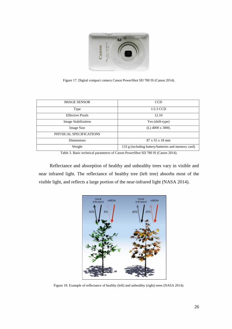
Reflectance and absorption of healthy and unhealthy trees vary in visible and

near infrared light. The reflectance of healthy tree (left tree) absorbs most of the

visible light, and reflects a large portion of the near-infrared light (NASA 2014).

Figure 18. Example of reflectance of healthy (left) and unhealthy (right) trees (NASA 2014).

27

Unhealthy trees (right tree) reflect more in visible light and less in near-

infrared light the numbers of reflectance/absorption, which is shown on the figure 18

are theoretical. The reflectance values can vary (NASA 2014).

Additionally, camera Canon PowerShot SD 780 IS was modified to be able to

capture not just visible spectrum (called hot mirror), but also NIR spectrum. The type

of conversion is UV + Visible + IR, it means that hot mirror of the camera was

removed. Now modified camera is able to capture radiation from about 330 nm to

1100 nm near infrared (Maxmax filter 2014). To restrict the captured spectrum of the

images the external filter was used, which blocks light of specific wavelengths. Self-

built cyan-filter was used, which blocks the visible red light. As result, the camera

records NIR light mainly as red, so we have colored infrared images with the bands

NIR/Green/Blue. All images are stored to the memory card of camera.

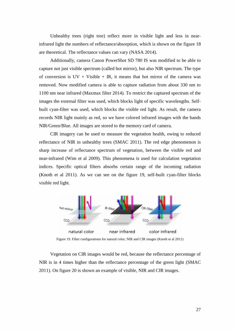
CIR imagery can be used to measure the vegetation health, owing to reduced

reflectance of NIR in unhealthy trees (SMAC 2011). The red edge phenomenon is

sharp increase of reflectance spectrum of vegetation, between the visible red and

near-infrared (Wim et al 2009). This phenomena is used for calculation vegetation

indices. Specific optical filters absorbs certain range of the incoming radiation

(Knoth et al 2011). As we can see on the figure 19, self-built cyan-filter blocks

visible red light.

Figure 19. Filter configurations for natural color, NIR and CIR images (Knoth et al 2011)

Vegetation on CIR images would be red, because the reflectance percentage of

NIR is in 4 times higher than the reflectance percentage of the green light (SMAC

2011). On figure 20 is shown an example of visible, NIR and CIR images.

28

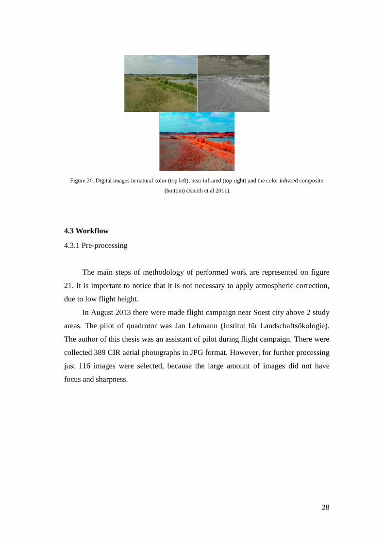
Figure 20. Digital images in natural color (top left), near infrared (top right) and the color infrared composite

(bottom) (Knoth et al 2011).

4.3 Workflow

4.3.1 Pre-processing

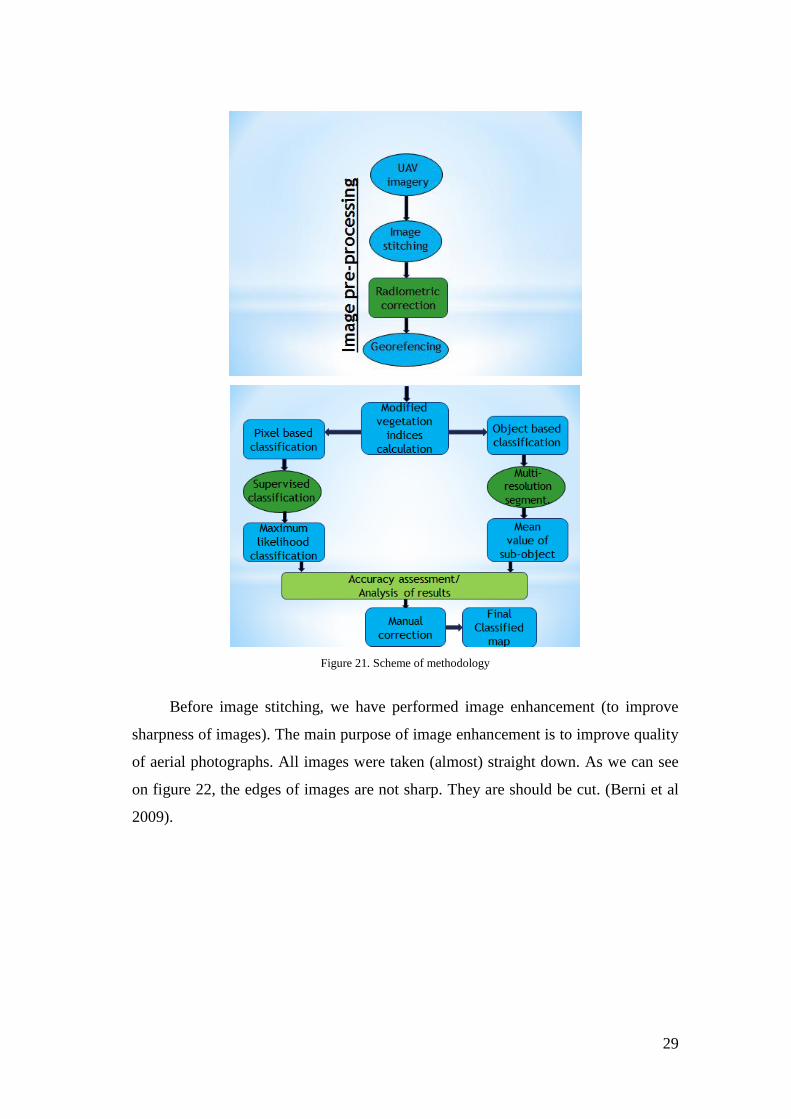
The main steps of methodology of performed work are represented on figure

21. It is important to notice that it is not necessary to apply atmospheric correction,

due to low flight height.

In August 2013 there were made flight campaign near Soest city above 2 study

areas. The pilot of quadrotor was Jan Lehmann (Institut für Landschaftsökologie).

The author of this thesis was an assistant of pilot during flight campaign. There were

collected 389 CIR aerial photographs in JPG format. However, for further processing

just 116 images were selected, because the large amount of images did not have

focus and sharpness.

29

Figure 21. Scheme of methodology

Before image stitching, we have performed image enhancement (to improve

sharpness of images). The main purpose of image enhancement is to improve quality

of aerial photographs. All images were taken (almost) straight down. As we can see

on figure 22, the edges of images are not sharp. They are should be cut. (Berni et al

2009).

30

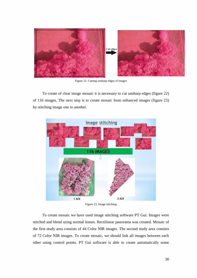
Figure 22. Cutting unsharp edges of images

To create of clear image mosaic it is necessary to cut unsharp edges (figure 22)

of 116 images. The next step is to create mosaic from enhanced images (figure 23)

by stitching image one to another.

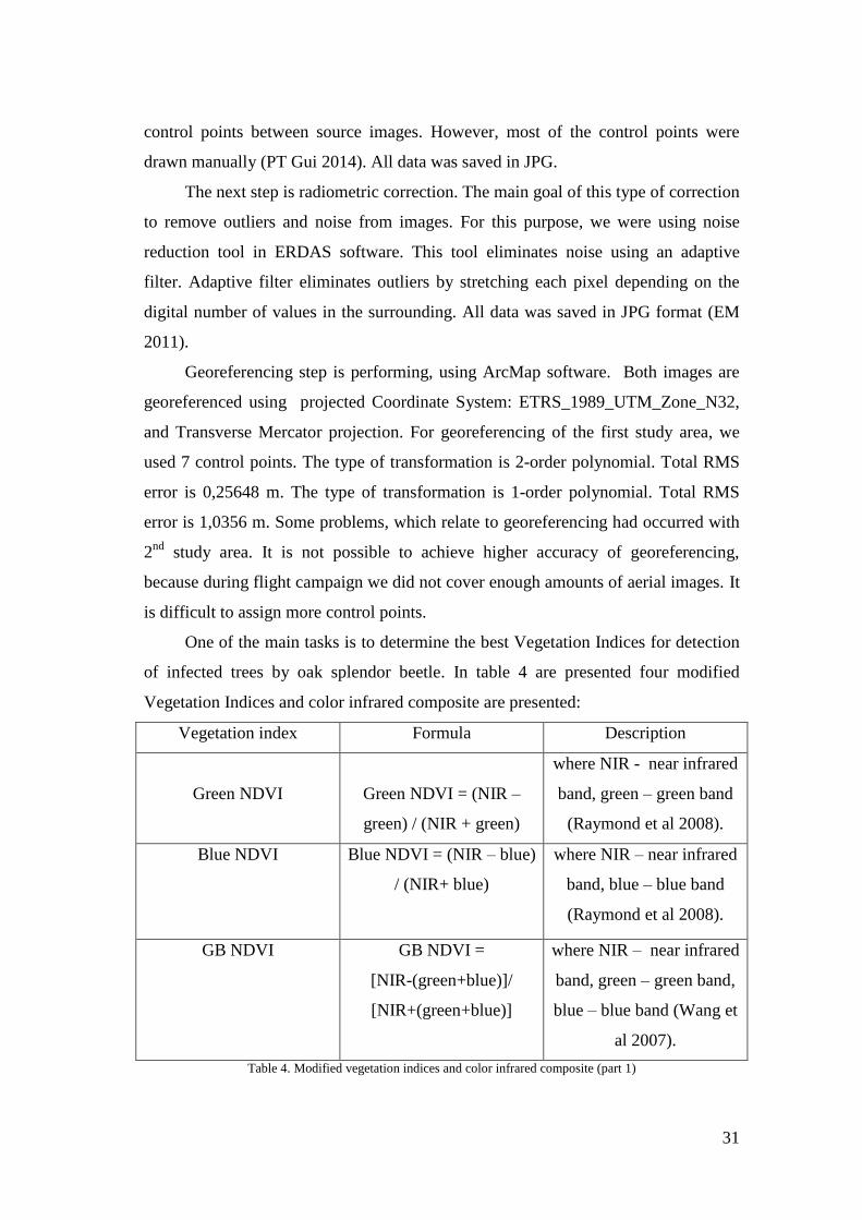
Figure 23. Image stitching

To create mosaic we have used image stitching software PT Gui. Images were

stitched and blend using normal lenses. Rectilinear panorama was created. Mosaic of

the first study area consists of 44 Color NIR images. The second study area consists

of 72 Color NIR images. To create mosaic, we should link all images between each

other using control points. PT Gui software is able to create automatically some

31

control points between source images. However, most of the control points were

drawn manually (PT Gui 2014). All data was saved in JPG.

The next step is radiometric correction. The main goal of this type of correction

to remove outliers and noise from images. For this purpose, we were using noise

reduction tool in ERDAS software. This tool eliminates noise using an adaptive

filter. Adaptive filter eliminates outliers by stretching each pixel depending on the

digital number of values in the surrounding. All data was saved in JPG format (EM

2011).

Georeferencing step is performing, using ArcMap software. Both images are

georeferenced using projected Coordinate System: ETRS_1989_UTM_Zone_N32,

and Transverse Mercator projection. For georeferencing of the first study area, we

used 7 control points. The type of transformation is 2-order polynomial. Total RMS

error is 0,25648 m. The type of transformation is 1-order polynomial. Total RMS

error is 1,0356 m. Some problems, which relate to georeferencing had occurred with

2nd

study area. It is not possible to achieve higher accuracy of georeferencing,

because during flight campaign we did not cover enough amounts of aerial images. It

is difficult to assign more control points.

One of the main tasks is to determine the best Vegetation Indices for detection

of infected trees by oak splendor beetle. In table 4 are presented four modified

Vegetation Indices and color infrared composite are presented:

Vegetation index Formula Description

Green NDVI

Green NDVI = (NIR –

green) / (NIR + green)

where NIR - near infrared

band, green – green band

(Raymond et al 2008).

Blue NDVI

Blue NDVI = (NIR – blue)

/ (NIR+ blue)

where NIR – near infrared

band, blue – blue band

(Raymond et al 2008).

GB NDVI GB NDVI =

[NIR-(green+blue)]/

[NIR+(green+blue)]

where NIR – near infrared

band, green – green band,

blue – blue band (Wang et

al 2007).

Table 4. Modified vegetation indices and color infrared composite (part 1)

32

GSAVI GSAVI = [(NIR – green) /

(NIR + green +L)] * (1 + L)

where NIR – near infrared

band, green – green band

L = 0.5 (VI, 2014)

color infrared

composite

(NIR, green, blue) NIR – near infrared band,

green – green band, blue –

blue band

Table 4. Modified vegetation indices and color infrared composite (part 2)

.

In remote sensing exist some problems of soil background effect (Huete 1988).

To reduce the soil background effect, (Huete 1988) one suggested to use a soil-

adjustment index (SAVI). Nevertheless, due to absence of red band we are using

GSAVI index. Color infrared composite (NIR, green, blue) data was used as well.

Principal component analysis was performed for both test sites. Principal

component analysis is a linear conversion technique. The main reason of using

principal component in remote sensing is to compress data by eliminating

redundancy (ArcGIS 2014). The first two or three principal components are capable

to highlighted original variability in reflectance values. Later principal components,

usually, are affected by noise (IDRISI 2014).

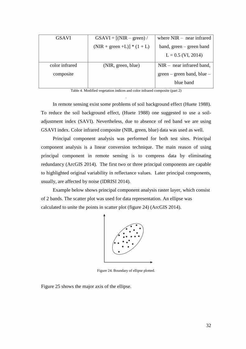
Example below shows principal component analysis raster layer, which consist

of 2 bands. The scatter plot was used for data representation. An ellipse was

calculated to unite the points in scatter plot (figure 24) (ArcGIS 2014).

Figure 24. Boundary of ellipse plotted.

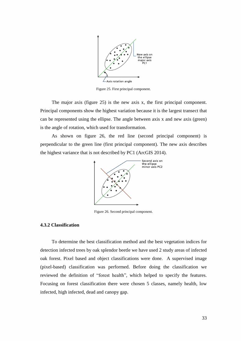
Figure 25 shows the major axis of the ellipse.

33

Figure 25. First principal component.

The major axis (figure 25) is the new axis x, the first principal component.

Principal components show the highest variation because it is the largest transect that

can be represented using the ellipse. The angle between axis x and new axis (green)

is the angle of rotation, which used for transformation.

As shown on figure 26, the red line (second principal component) is

perpendicular to the green line (first principal component). The new axis describes

the highest variance that is not described by PC1 (ArcGIS 2014).

Figure 26. Second principal component.

4.3.2 Classification

To determine the best classification method and the best vegetation indices for

detection infected trees by oak splendor beetle we have used 2 study areas of infected

oak forest. Pixel based and object classifications were done. A supervised image

(pixel-based) classification was performed. Before doing the classification we

reviewed the definition of “forest health”, which helped to specify the features.

Focusing on forest classification there were chosen 5 classes, namely health, low

infected, high infected, dead and canopy gap.

34

4.3.2.1 Pixel based classification

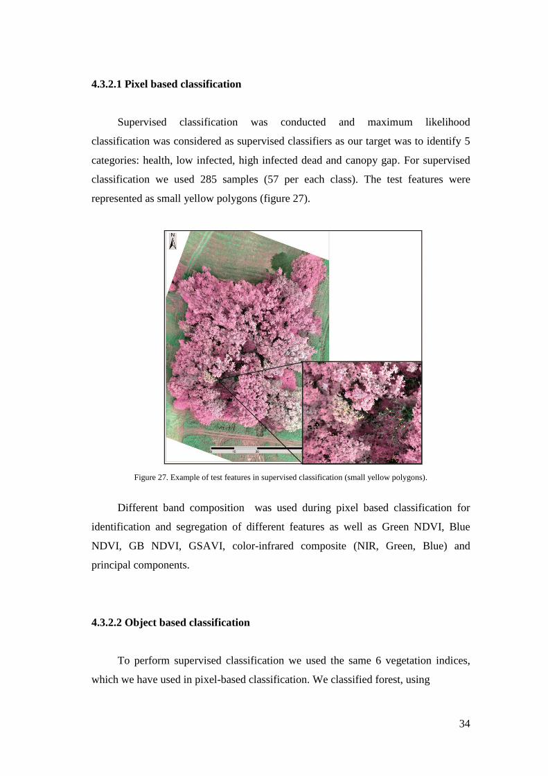
Supervised classification was conducted and maximum likelihood

classification was considered as supervised classifiers as our target was to identify 5

categories: health, low infected, high infected dead and canopy gap. For supervised

classification we used 285 samples (57 per each class). The test features were

represented as small yellow polygons (figure 27).

Figure 27. Example of test features in supervised classification (small yellow polygons).

Different band composition was used during pixel based classification for

identification and segregation of different features as well as Green NDVI, Blue

NDVI, GB NDVI, GSAVI, color-infrared composite (NIR, Green, Blue) and

principal components.

4.3.2.2 Object based classification

To perform supervised classification we used the same 6 vegetation indices,

which we have used in pixel-based classification. We classified forest, using

35

5 classes: health, low infected, high infected dead and canopy gaps. Ecogntion

software was used to perform object based classification. The first step in object-

based classification is multi-resolution segmentation based on scale, color and

compactness. They have the following values scale – 230, color – 0.6, and

compactness – 0.5. Then classification was conducted based on mean values of sub-

objects. These values are experimentally determined and represented the best results

of image segmentation on trees level. The output data were stored in raster format.

4.3.3 Post-processing

Post-processing step consists of the 2 parts: image enhancement, by applying

majority filter and manual correction of the best-classified image. Majority filter was

applied just for pixel-based classified images. The filter can be used for either

elimination spurious data or enhance data by reducing local variation, removing

noise and others (AHFW 2014).

Majority filters replaces cells in a raster data based on the majority of their

contiguous neighboring cells. The output data were stored in raster format (MF

2014). Number of the neighbors is eight. Majority method was chosen as

replacement threshold.

After comparison of pixel and object-based classified images, it was defined

that the best vegetation index for detection of infected trees is GB NDVI vegetation

index (object-based classification). GB NDVI index was manually improved in order

to create final maps for the both study areas.

4.4 Accuracy assessment

Performing of accuracy assessment is important to determine an error, and

results interpretation. Overall accuracy, producer’s accuracy, user’s accuracy and

Kappa coefficient are the most famous accuracy assessment elements. In this work

were calculated error matrix and kappa statistic. The error matrix (correlation matrix

36

or covariance matrix) is the sum between two datasets, which usually compare

classification maps, images and others (UofA 2004).

An error matrix allows to access of accuracy of single remote sensing image. The

error matrix is the most common method for accuracy assessment. Other accuracy

assessment components, for instance, overall accuracy, producer’s accuracy, user’s

accuracy can be developed using the error matrix.

Producer's accuracy is a measure of accuracy, when the total number of pixel in

a group is divided by the total number of pixel of that group, which extracted from

ground truth data. It has a name “producer’s” accuracy, because the producer of the

classification can identify how well a particular area will be classified. User's

accuracy is a measure of accuracy, when the total number of correct pixels in a group

is divided by the total number of pixels that were classified in that group (Congalton

1991). Another technique used in accuracy assessment is Kappa analysis. Kappa

statistic is measure of agreement (accuracy), which based on the difference between

the actual agreements in the error matrix (equation 5).

(5)

where n – number of samples, - sum of correct classified samples, -

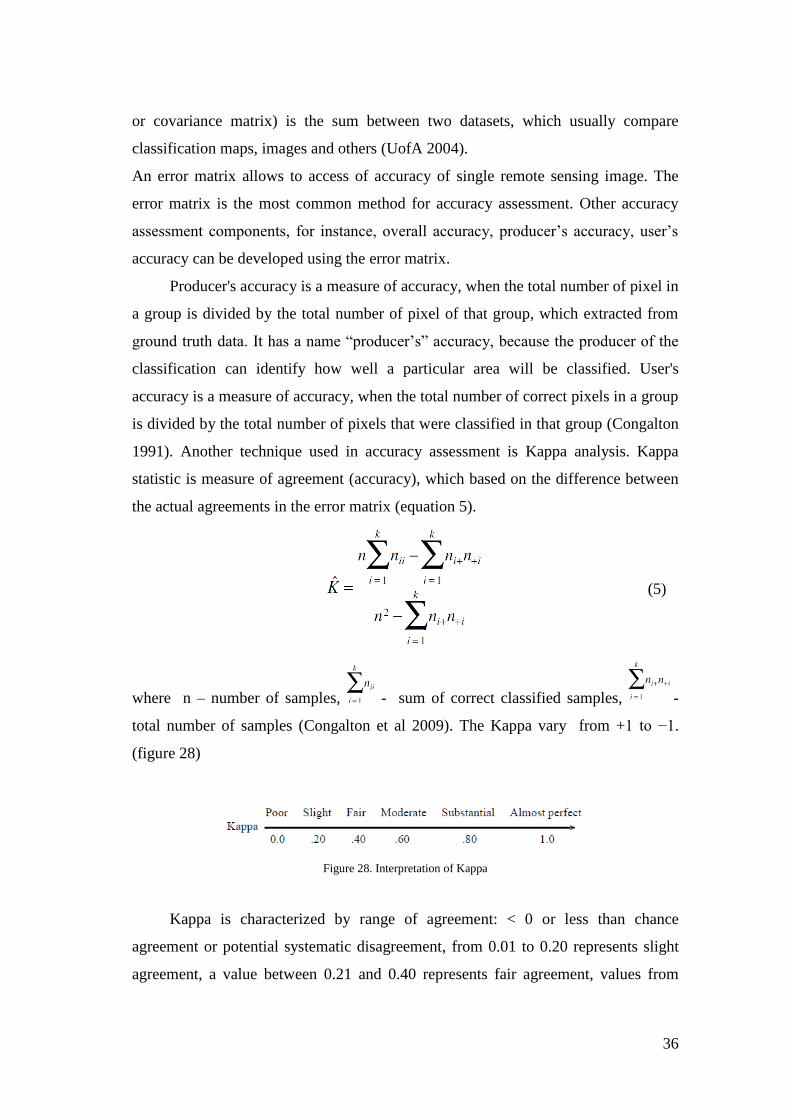
total number of samples (Congalton et al 2009). The Kappa vary from +1 to −1.

(figure 28)

Figure 28. Interpretation of Kappa

Kappa is characterized by range of agreement: < 0 or less than chance

agreement or potential systematic disagreement, from 0.01 to 0.20 represents slight

agreement, a value between 0.21 and 0.40 represents fair agreement, values from

37

0.41 to 0.60 represent moderate agreement, 0.61–0.80 demonstrate substantial

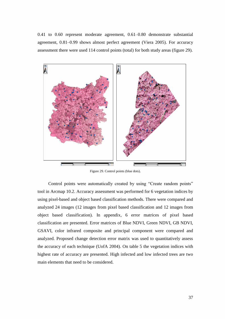
agreement, 0.81–0.99 shows almost perfect agreement (Viera 2005). For accuracy

assessment there were used 114 control points (total) for both study areas (figure 29).

Figure 29. Control points (blue dots).

Control points were automatically created by using “Create random points”

tool in Arcmap 10.2. Accuracy assessment was performed for 6 vegetation indices by

using pixel-based and object based classification methods. There were compared and

analyzed 24 images (12 images from pixel based classification and 12 images from

object based classification). In appendix, 6 error matrices of pixel based

classification are presented. Error matrices of Blue NDVI, Green NDVI, GB NDVI,

GSAVI, color infrared composite and principal component were compared and

analyzed. Proposed change detection error matrix was used to quantitatively assess

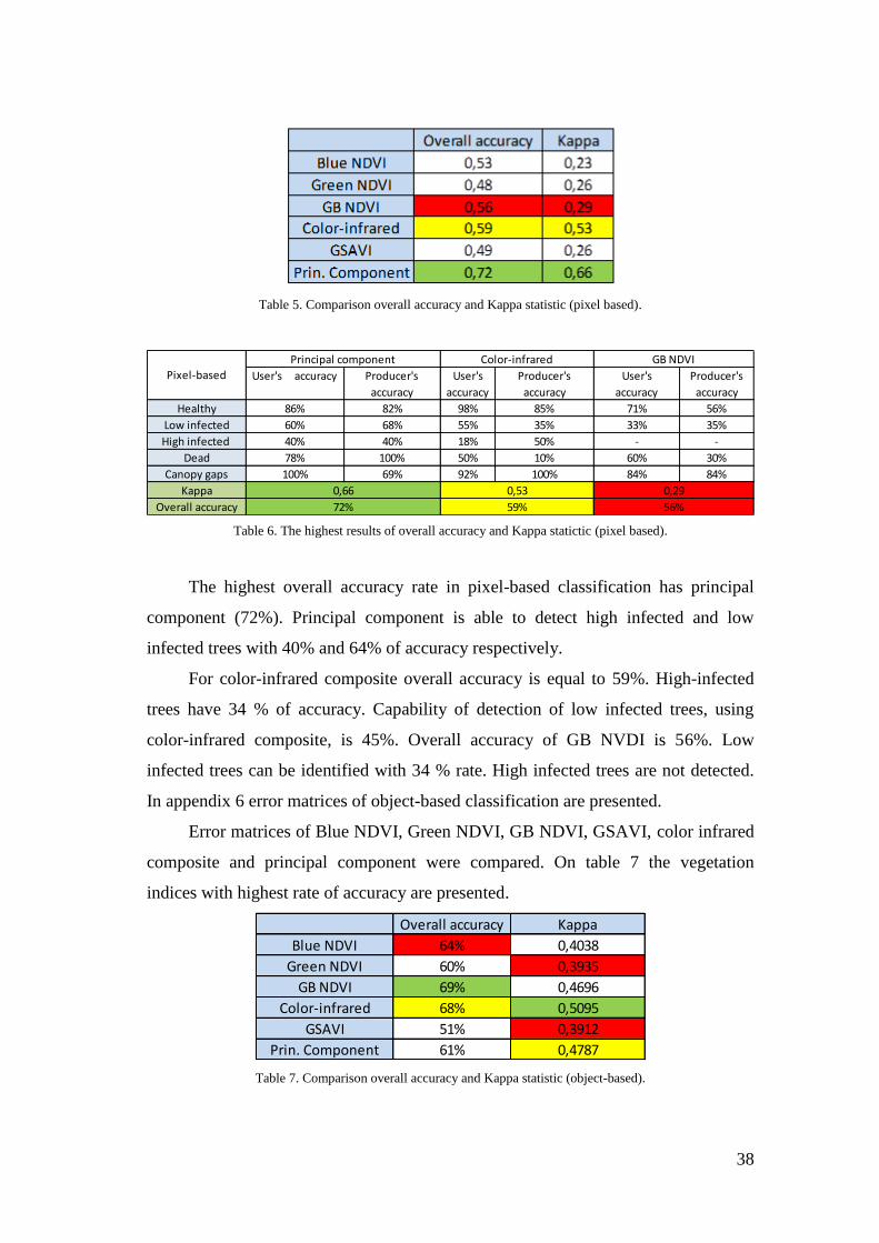
the accuracy of each technique (UofA 2004). On table 5 the vegetation indices with

highest rate of accuracy are presented. High infected and low infected trees are two

main elements that need to be considered.

38

Table 5. Comparison overall accuracy and Kappa statistic (pixel based).

User's accuracy Producer's

accuracy

User's

accuracy

Producer's

accuracy

User's

accuracy

Producer's

accuracy

Healthy 86% 82% 98% 85% 71% 56%

Low infected 60% 68% 55% 35% 33% 35%

High infected 40% 40% 18% 50% - -

Dead 78% 100% 50% 10% 60% 30%

Canopy gaps 100% 69% 92% 100% 84% 84%

Kappa

Overall accuracy 72% 59% 56%

Pixel-based

Principal component Color-infrared GB NDVI

0,66 0,53 0,29

Table 6. The highest results of overall accuracy and Kappa statictic (pixel based).

The highest overall accuracy rate in pixel-based classification has principal

component (72%). Principal component is able to detect high infected and low

infected trees with 40% and 64% of accuracy respectively.

For color-infrared composite overall accuracy is equal to 59%. High-infected

trees have 34 % of accuracy. Capability of detection of low infected trees, using

color-infrared composite, is 45%. Overall accuracy of GB NVDI is 56%. Low

infected trees can be identified with 34 % rate. High infected trees are not detected.

In appendix 6 error matrices of object-based classification are presented.

Error matrices of Blue NDVI, Green NDVI, GB NDVI, GSAVI, color infrared

composite and principal component were compared. On table 7 the vegetation

indices with highest rate of accuracy are presented.

Overall accuracy Kappa

Blue NDVI 64% 0,4038

Green NDVI 60% 0,3935

GB NDVI 69% 0,4696

Color-infrared 68% 0,5095

GSAVI 51% 0,3912

Prin. Component 61% 0,4787

Table 7. Comparison overall accuracy and Kappa statistic (object-based).

39

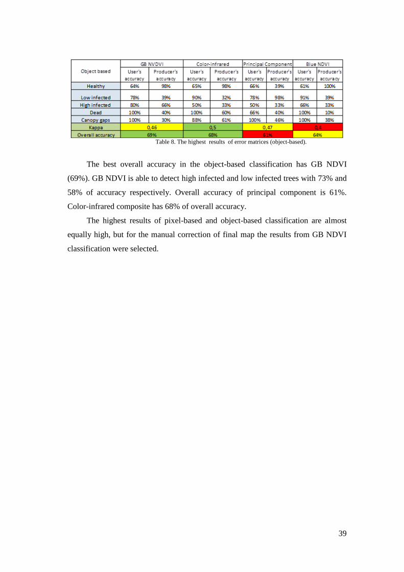
Table 8. The highest results of error matrices (object-based).

The best overall accuracy in the object-based classification has GB NDVI

(69%). GB NDVI is able to detect high infected and low infected trees with 73% and

58% of accuracy respectively. Overall accuracy of principal component is 61%.

Color-infrared composite has 68% of overall accuracy.

The highest results of pixel-based and object-based classification are almost

equally high, but for the manual correction of final map the results from GB NDVI

classification were selected.

40

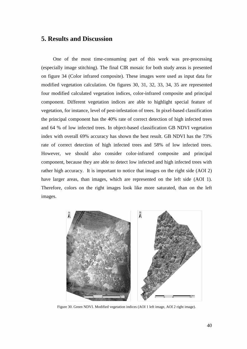
5. Results and Discussion

One of the most time-consuming part of this work was pre-processing

(especially image stitching). The final CIR mosaic for both study areas is presented

on figure 34 (Color infrared composite). These images were used as input data for

modified vegetation calculation. On figures 30, 31, 32, 33, 34, 35 are represented

four modified calculated vegetation indices, color-infrared composite and principal

component. Different vegetation indices are able to highlight special feature of

vegetation, for instance, level of pest-infestation of trees. In pixel-based classification

the principal component has the 40% rate of correct detection of high infected trees

and 64 % of low infected trees. In object-based classification GB NDVI vegetation

index with overall 69% accuracy has shown the best result. GB NDVI has the 73%

rate of correct detection of high infected trees and 58% of low infected trees.

However, we should also consider color-infrared composite and principal

component, because they are able to detect low infected and high infected trees with

rather high accuracy. It is important to notice that images on the right side (AOI 2)

have larger areas, than images, which are represented on the left side (AOI 1).

Therefore, colors on the right images look like more saturated, than on the left

images.

Figure 30. Green NDVI. Modified vegetation indices (AOI 1 left image, AOI 2 right image).

41

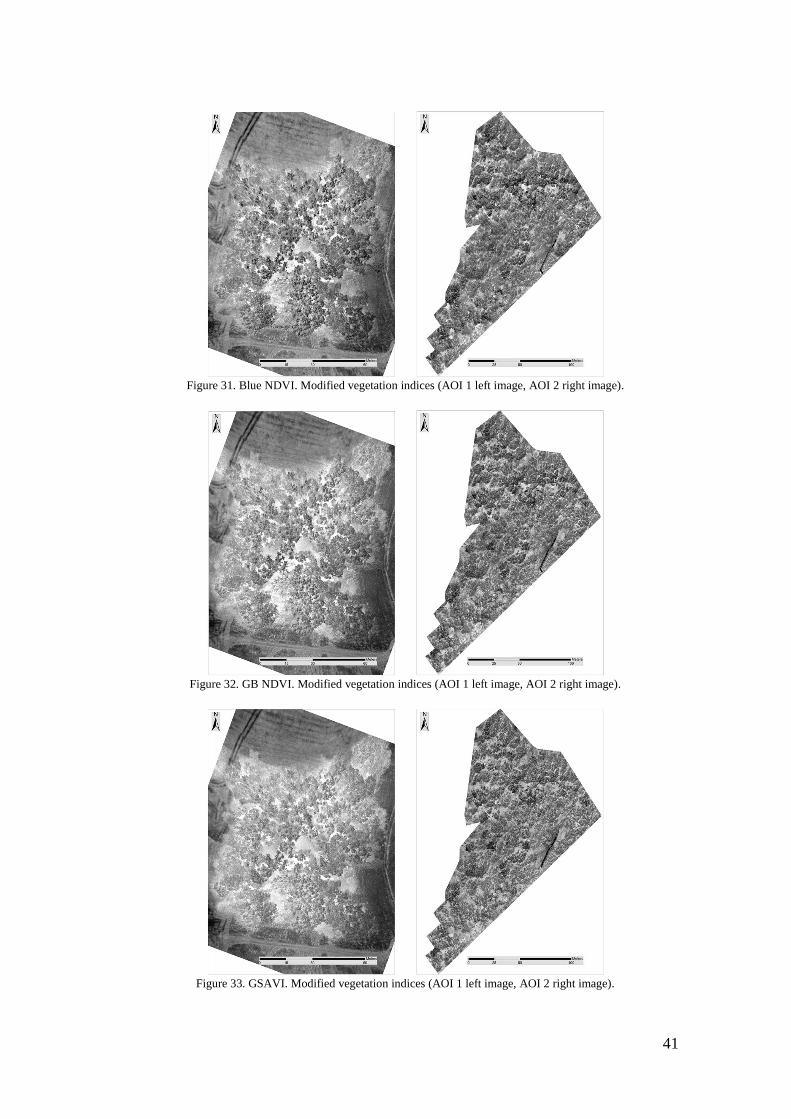
Figure 31. Blue NDVI. Modified vegetation indices (AOI 1 left image, AOI 2 right image).

Figure 32. GB NDVI. Modified vegetation indices (AOI 1 left image, AOI 2 right image).

Figure 33. GSAVI. Modified vegetation indices (AOI 1 left image, AOI 2 right image).

42

Figure 34. Color-infrared composite (AOI 1 left image, AOI 2 right image).

Figure 35. Principal component (AOI 1 left image, AOI 2 right image).

Infected trees on Green NDVI, GSAVI images are represented in saturated

black color, while canopy gaps are represented in white color. On Blue NDVI

images, it is problematically to identify infected trees visually. On the GB NDVI

images, generally, infected oak trees are marked as the darkest areas. On the color-

infrared images it is easy to identify healthy, high infected, low infected, died trees

and canopy gaps. Healthy trees are represented in saturated red color. Infected trees

are shown by nankeen color. We can identify died branches and tree trunk by black

color. Finally, infected trees are marked by violet color on principal component

images. Healthy trees are represented by reddish color.

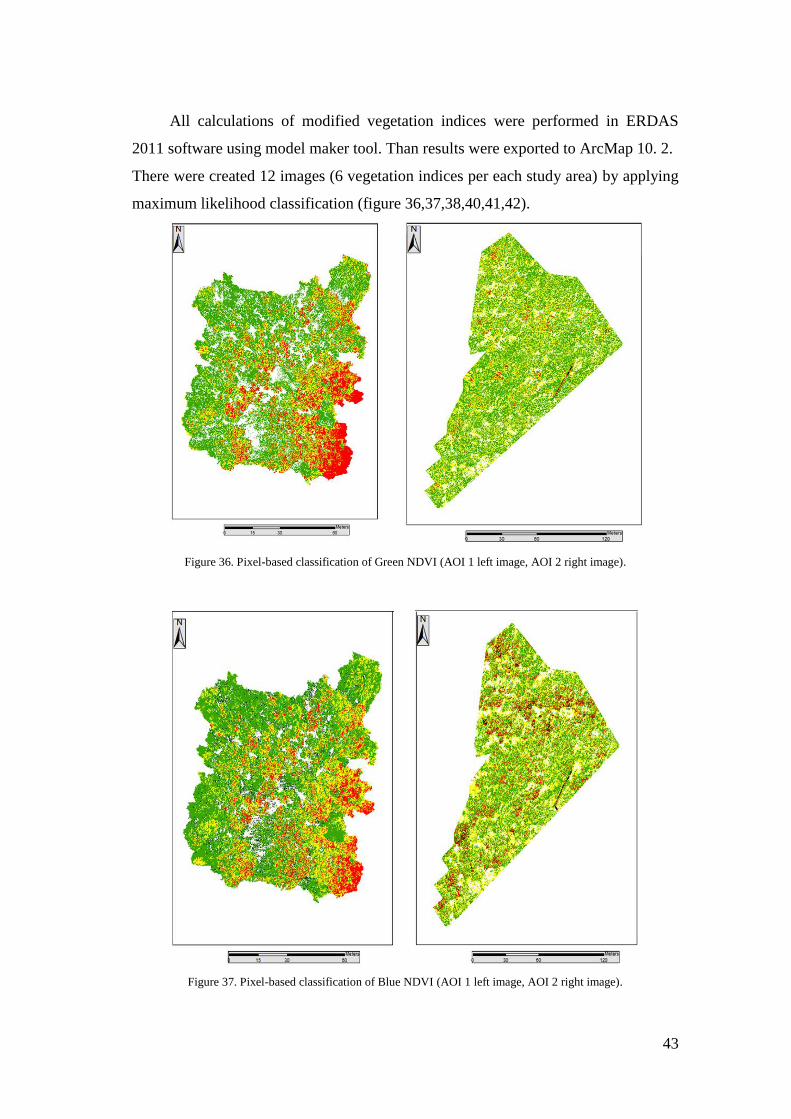
43

All calculations of modified vegetation indices were performed in ERDAS

2011 software using model maker tool. Than results were exported to ArcMap 10. 2.

There were created 12 images (6 vegetation indices per each study area) by applying

maximum likelihood classification (figure 36,37,38,40,41,42).

Figure 36. Pixel-based classification of Green NDVI (AOI 1 left image, AOI 2 right image).

Figure 37. Pixel-based classification of Blue NDVI (AOI 1 left image, AOI 2 right image).

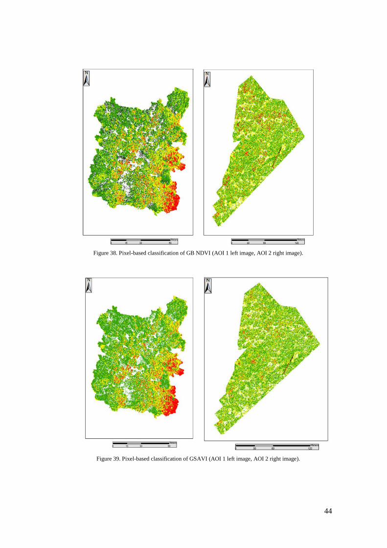
44

Figure 38. Pixel-based classification of GB NDVI (AOI 1 left image, AOI 2 right image).

Figure 39. Pixel-based classification of GSAVI (AOI 1 left image, AOI 2 right image).

45

Figure 40. Pixel-based classification of color-infrared composite (AOI 1 left image, AOI 2 right image).

Figure 41. Pixel-based classification of principal component analysis (AOI 1 left image, AOI 2 right image).

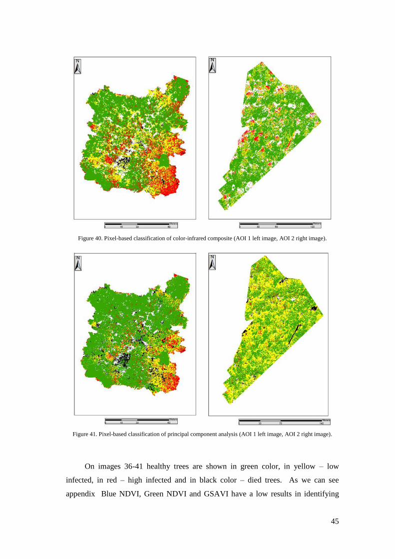
On images 36-41 healthy trees are shown in green color, in yellow – low

infected, in red – high infected and in black color – died trees. As we can see

appendix Blue NDVI, Green NDVI and GSAVI have a low results in identifying

46

died trees. The best results of detecting died trees and overall accuracy have principal

component. The main disadvantage of pixel-based classification is that the class is

determined by single pixel, without considering information of neighbor pixels.

Therefore, whole tree can be misclassified based on information of single pixel.

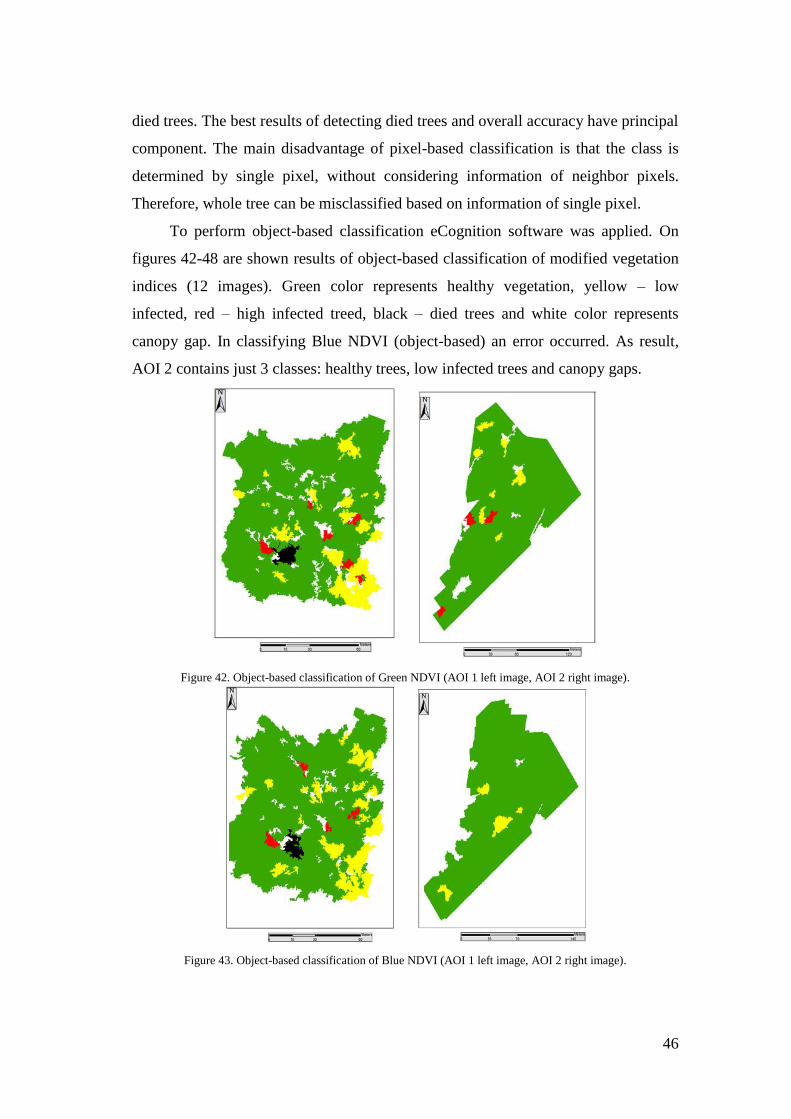
To perform object-based classification eCognition software was applied. On

figures 42-48 are shown results of object-based classification of modified vegetation

indices (12 images). Green color represents healthy vegetation, yellow – low

infected, red – high infected treed, black – died trees and white color represents

canopy gap. In classifying Blue NDVI (object-based) an error occurred. As result,

AOI 2 contains just 3 classes: healthy trees, low infected trees and canopy gaps.

Figure 42. Object-based classification of Green NDVI (AOI 1 left image, AOI 2 right image).

Figure 43. Object-based classification of Blue NDVI (AOI 1 left image, AOI 2 right image).

47

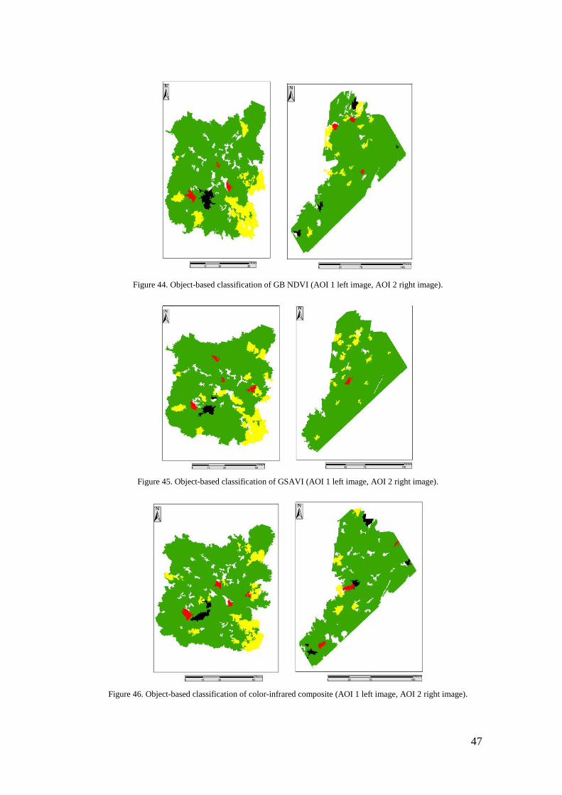
Figure 44. Object-based classification of GB NDVI (AOI 1 left image, AOI 2 right image).

Figure 45. Object-based classification of GSAVI (AOI 1 left image, AOI 2 right image).

Figure 46. Object-based classification of color-infrared composite (AOI 1 left image, AOI 2 right image).

48

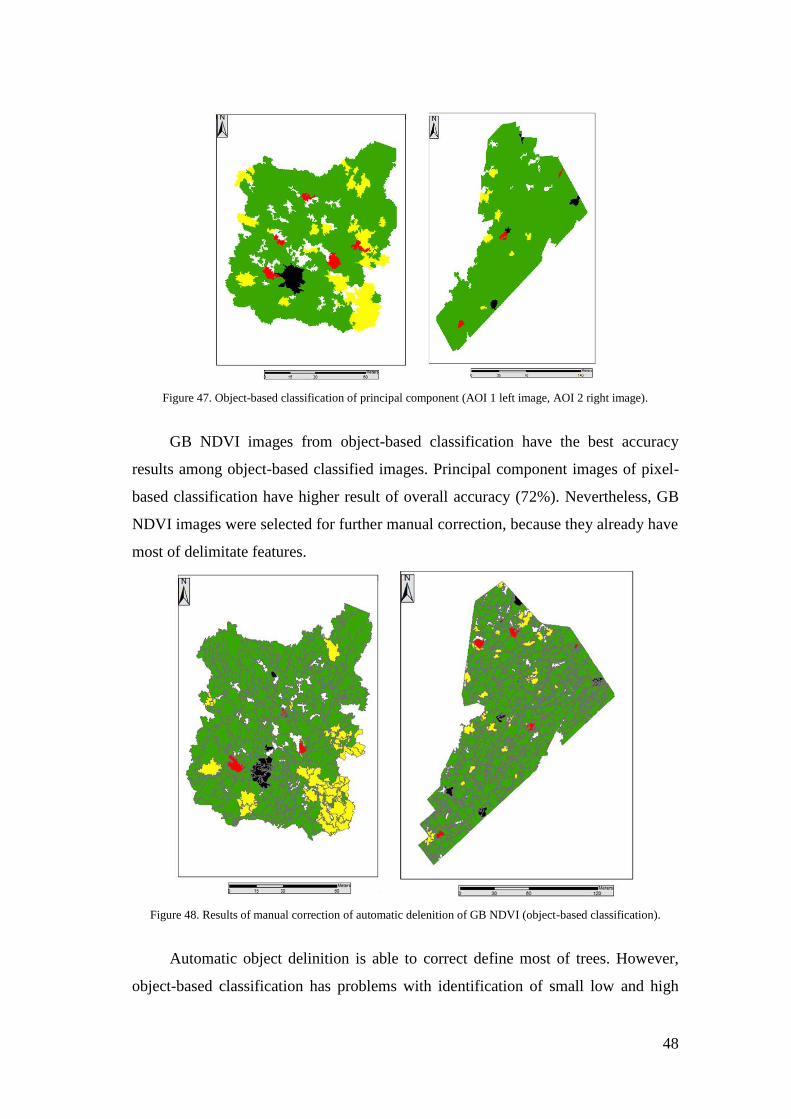
Figure 47. Object-based classification of principal component (AOI 1 left image, AOI 2 right image).

GB NDVI images from object-based classification have the best accuracy

results among object-based classified images. Principal component images of pixel-

based classification have higher result of overall accuracy (72%). Nevertheless, GB

NDVI images were selected for further manual correction, because they already have

most of delimitate features.

Figure 48. Results of manual correction of automatic delenition of GB NDVI (object-based classification).

Automatic object delinition is able to correct define most of trees. However,

object-based classification has problems with identification of small low and high

49

infected trees. Small trees were detected by comparison with color-infrared

composite.

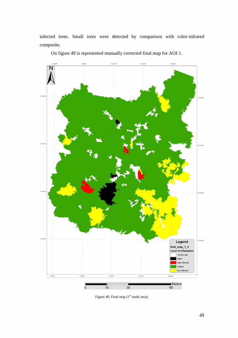
On figure 49 is represented manually corrected final map for AOI 1.

Figure 49. Final map (1st study area).

50

As we can see on figure 49 most of the area is covered by healthy vegetation.

There are 3 died trees (2 in the centre of image and on the top of image).

Furthermore, 3 high infected trees are located in centre of 1st study area. On the

lower right corner, according to classification, low infected trees are located. This

results may be influenced by position of the sun. The flight campaign for AOI 1was

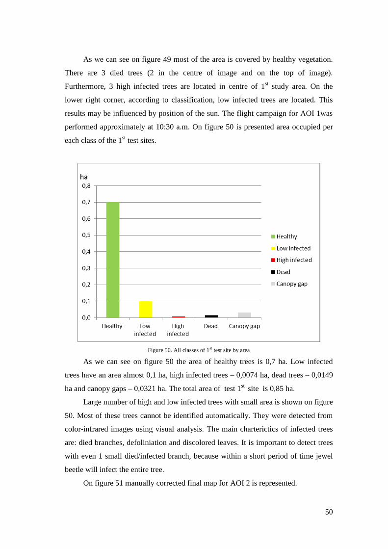
performed approximately at 10:30 a.m. On figure 50 is presented area occupied per

each class of the 1st test sites.

Figure 50. All classes of 1st test site by area

As we can see on figure 50 the area of healthy trees is 0,7 ha. Low infected

trees have an area almost 0,1 ha, high infected trees – 0,0074 ha, dead trees – 0,0149

ha and canopy gaps – 0,0321 ha. The total area of test 1st

site is 0,85 ha.

Large number of high and low infected trees with small area is shown on figure

50. Most of these trees cannot be identified automatically. They were detected from

color-infrared images using visual analysis. The main charterictics of infected trees

are: died branches, defoliniation and discolored leaves. It is important to detect trees

with even 1 small died/infected branch, because within a short period of time jewel

beetle will infect the entire tree.

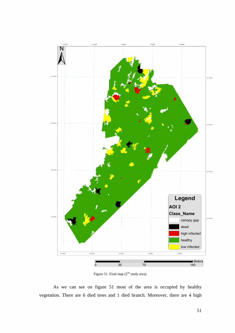
On figure 51 manually corrected final map for AOI 2 is represented.

51

Figure 51. Final map (2nd study area).

As we can see on figure 51 most of the area is occupied by healthy

vegetation. There are 6 died trees and 1 died branch. Moreover, there are 4 high

52

infected trees and 7 small high infected branches. On figure 51 it is possible to detect

22 low infected trees and 4 low infected branches. The flight campaign was

performed at 12:30 p.m. Therefore, the results for 2nd

study area is less influenced

by effect of sun illumination. The results more accurate, especially for low infected

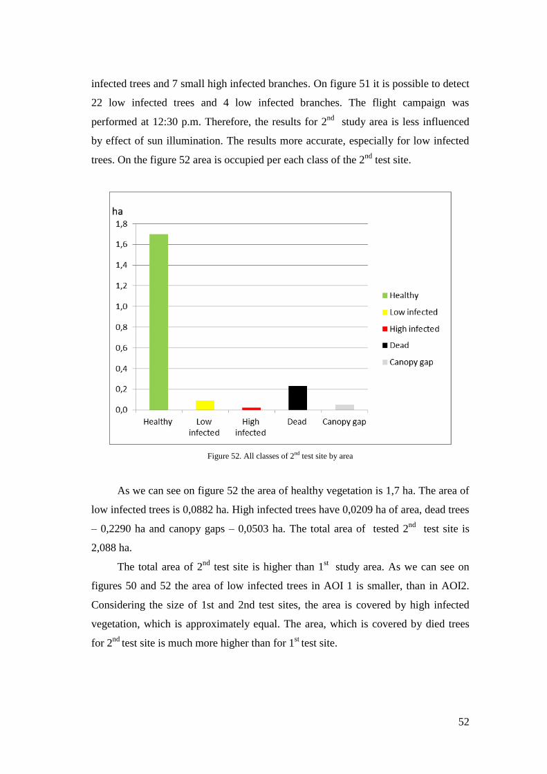
trees. On the figure 52 area is occupied per each class of the 2nd

test site.

Figure 52. All classes of 2nd test site by area

As we can see on figure 52 the area of healthy vegetation is 1,7 ha. The area of

low infected trees is 0,0882 ha. High infected trees have 0,0209 ha of area, dead trees

– 0,2290 ha and canopy gaps – 0,0503 ha. The total area of tested 2nd

test site is

2,088 ha.

The total area of 2nd

test site is higher than 1st

study area. As we can see on

figures 50 and 52 the area of low infected trees in AOI 1 is smaller, than in AOI2.

Considering the size of 1st and 2nd test sites, the area is covered by high infected

vegetation, which is approximately equal. The area, which is covered by died trees

for 2nd

test site is much more higher than for 1st

test site.

53

The obtained results will be send to Soest forest agency for integration with

existing WMS service. Results from two experimental sites are shown; UAV

imagery can be useful tool for detection and monitoring of pest-infected trees.

54

5. CONCLUSION

The results of this work demonstrated that it was possible to identify the level

of pest infestation of oak’s trees, by using UAV very high resolution imagery.

Traditionally, the medium and high resolution imagery are used in forestry. By

applying UAV imagery were determined classes of pest infected trees and vegetation

indices.

The proposed workflow in this work included the CIR image acquisition,

image stitching, radiometric correction, georeferencing, modified vegetation indices

calculation, pixel-based and object-based image classification and accuracy

assessment. Images were classified using 5 classes (healthy, low infected, high

infected, and died trees and canopy gaps).

The analysis of classification showed that principal component (pixel-based)

had the highest overall accuracy (75%), and higher accuracy in detection of low

infected trees, than object-based classification (GB NDVI 72%). As well good result

of overall accuracy had color-infrared composite (60%) in pixel-based classification,

and principal component (64%), color-infrared composite (62%) in object-based

classification. Generally, object-based classification method is known as a method,

which usually has higher accuracy than pixel-based classification. Almost equal

results for pixel-based and object-based classification may depend on small amount

of control points (114). Therefore it is necessary to increase the number of control

points in subsequent work. Future studies for this area will consider different time

intervals, which allow comparing images and detect annual changes of pest-

infestation. UAV was beneficial for forest health monitoring and for registering of

changes. It is important to use additional characteristics for object-based

classification, such as texture, shape and others.

For future studies it is important to use geodetic GPS (with real time kinematic

technique) for achieving higher accuracy during GPS points collection. Accurate

ground truth data is necessary for successful infected trees identification using UAV.

Also, meaningful results might be obtained using multispectral camera, with at least

4 bands.

55

BIBLIOGRAPHIC REFERENCES

AHFW, (2014). How filter works. Date of access 04.01.2014. Website of the

ArcGIS.

http://resources.arcgis.com/en/help/main/10.1/index.html#//009z000000r50000

00

ArcGIS, (2014). How Principal Components works. Date of access 12.01.2014.

Website of the ArcGIS.

http://help.arcgis.com/en/arcgisdesktop/10.0/help/index.html#/How_Principal_

Components_works/009z000000qm000000/

BERNI J., ZARCO-TEJADA P., SUAREZ L., GONZALEZ-DUGO V., FERERES

E., (2009). Remote sensing of vegetation from UAV platforms using

lightweight multispectral and thermal imaging sensors.

BÜRO, (2008). Büro für Wald- und Umweltplanung Leonhardt. Betriebswerk für

die Forstbetriebsgemeinschaft Lippetal.

CANON, (2014). Date of access 14.01.2014. Website of the Imaging resource.

http://www.imaging-resource.com/PRODS/SD780IS/SD780ISA.HTM

CONGALTON R., (1991). A Review of Assessing the Accuracy of Classifications

of Remotely Sensed Data. Remote sensing environment. (37) pp. 35-46.

CONGALTON R., GREEN K., (2009). Assessing the Accuracy of Remotely Sensed

Data Principles and Practices. Second Edition. pp. 105-110.

CRSI, (2014). Date of access 27.12.2013. Website of the center for remote sensing

imaging. http://www.crisp.nus.edu.sg/~research/tutorial/image.htm

DAVID W., CASBEER S., RANDAL W., BEARD R., MCLAIN T., (2005). Forest

Fire Monitoring With Multiple Small UAVs. American Control Conference

June 8-10, 2005. Portland, OR, USA.

EM, (2011). ERDAS Field Guide (5th edition). pp. 139. Access on 17.11.2013

http://www.gis.usu.edu/manuals/labbook/erdas/manuals/FieldGuide.pdf

DOA, (2014). Department of agriculture. Oak splendor Beetle. Date of access

29.01.2014. Website of the center

http://www.agri.ohio.gov/divs/plant/caps/docs/osb.pdf

56

DUZGUN H., DEMIREL N. (2011), Remote Sensing of the Mine Environment. pp

67-71.

GARMIN, (2014). GPS Owner Manual. Date of access 24.01.2014. Website of the

manufacturer. pp. 40.

http://static.garmincdn.com/pumac/GPSMAP62_OM_EN.pdf

GE, (2014). Date of access 09.12.2013. Google Earth software.

http://www.google.com/earth/explore/products/desktop.html

GRENZDÖRFFER G., ENGELB A., TEICHERTC B., (2008). The photogrammetric

potential of low-cost UAVs in forestry and agriculture. The International

Archives of the Photogrammetry, Remote Sensing and Spatial Information

Sciences. Vol. XXXVII. Part B1.

HORCHER, A. and VISSER R., (2004). Unmanned Aerial Vehicles: Applications

for Natural Resource Management and Monitoring.- COFE (Council on Forest

Engineering) Annual Meeting Proceedings.

HUETE, A. (1988). A soil-adjusted vegetation index (SAVI), Remote Sensing.

Environment. 25. pp. 295-309.

HUNG C., BRYSON M., SUKKARIEH S., (2012). Multi-class predictive template

for tree crown detection. ISPRS Journal of Photogrammetry and Remote

Sensing 68 (2012) pp. 170–183

IDRISI, (2014). IDRISI Guide to GIS and Image Processing Volume 1. page 17.

Date of access 17.11.2013.

https://www.mtholyoke.edu/courses/tmillett/course/geog205/files/remote_sensi

ng.pdf

KNOTH, C., PRINZ, T. LOEF, P., (2011). Microcopter-based Color Infrared (CIR)

close range remote sensing as a subsidiary tool for precision farming. In:

Proceedings of the Workshop on Remote Sensing Methods for Change

Detection and Process Modeling, pp. 49–54. 18–19 November 2010, Cologne,

DE.

LALIBERTE A., RANGO A., (2009). Texture and Scale in Object-Based Analysis

of Subdecimeter Resolution Unmanned Aerial Vehicle (UAV) Imagery. IEEE

Transactions on geoscience and remote sensing. Vol. 47 (3). pp. 761-770

57

LINDQUIST E., D’ANNUNZIO R., GERRAND A., MACDICKEN K., ACHARD

F., BEUCHLE R., BRINK A., EVA H., MAYAUX P., SAN-MIGUEL-

AYANZ J. AND STIBIG H., (2012). Global forest land-use change 1990–

2005, Food and agriculture organization of the united nations, Rome, pp.11.

MF, (2014). Majority Filter. Website of the ArcGIS. Date of access 10.02.2014.

http://help.arcgis.com/en/arcgisdesktop/10.0/help/index.html#//009z000000370

00000.htm

MICRODRONE, 2014. Website of the microdrone company. Date of access

15.02.2014. http://www.microdrones.com/wiki/index.php/md4-200

MILAN Z., (2014). Forest Research Institute – Slovakia. Date of access 25.01.2014.

http://www.insectimages.org/browse/detail.cfm?imgnum=5378034#sthash.iMp

Y9gCq.dpuf

NASA, (2014). NASA Earth Observatory. Date of access 11.02.2014.

http://earthobservatory.nasa.gov/Features/MeasuringVegetation/measuring_veg

etation_2.php

NOMA T., COLUNGA-GARCIA M., BREWER M., LANDIS J., GOOCH A. an

PHILIP M., (2010). Oak splendor beetle Agrilus biguttatus. Michigan State

University IPM Program and of Michigan Department of Agriculture.

MAXMAX FILTER, (2014). Conversion. Date of access 15.02.2014. Website of the

maxmax company. Date of access 10.10.2013.

http://www.maxmax.com/ircameraconversions.htm

OOC, (2014). Object-Oriented Image Classification Methods. Website of the

Pennsylvania State University. Date of access 02.12.2013. https://www.e-

education.psu.edu/geog883kls/node/523

OM. Openstreet map, (2014). Date of access 14.09.2013.

http://www.openstreetmap.org/

PT GUI, (2014). Projections PT Gui. http://www.ptgui.com/man/projections.html

RAYMOND E., HIVELY W., DAUGHTRY C., MCCARTY C., (2008). Remote

sensing of crop leaf area index using unmanned airborne vehicles. The Future

of Land Imaging. November 18 – 20, 2008 Denver, Colorado.

58

RAZA S., GUEAIEB W., (2010). Intelligent Flight Control of an Autonomous

Quadrotor. University of Ottawa, Canada. p. 3.

REIßMANN K., 2010. The Jewel beetle. Website of beetle fauna of Germany. Date

of access 03.10.2013.

http://www.kerbtier.de/Pages/Themenseiten/enAgrilus.html

SMAC. Statewide Mapping Advisory Committee, (2011). Using Color Infrared

(CIR) Imagery a Guide for Understanding, Interpreting and Benefiting from

CIR Imagery. pp. 7, 16.

SKRZYPIETZ T., (2012). Unmanned Aircraft Systems for Civilian Missions. BIGS

Policy Paper 1. (February). pp. 6-7.

SOLOVIOV O., KNOTH C., PRINZ T., LEHMANN J., (2014). UAS-based High-

Resolution CIR Image Analysis to Detect Pest Infestation in Forestry. Poster.

European Geosciences Union.(In press).

TUOMINEN J., LIPPING T., KUOSMANEN V. HAAPANEN R., (2009).

Remote Sensing of Forest Health, Geoscience and Remote Sensing, pp. 29-52.

UDELHOVEN T., (2012). The use of an UAV as a remote sensing platform in

agricultural Applications. BMR Forum Luxinnovation.

UofA, (2004). Error Matrix for Map Comparison or Accuracy Assessment, UofA

Biological Sciences – GIS.

http://www.biology.ualberta.ca/gis/uploads/instructions/AVErrorMatrix.pdf

VALAVANIS K., (2007). Design and Control of a Miniature

Quadrotor. Intelligent systems, control, and automation, volume 33. pp. 174.

VIERA A., GARRETT J., (2005). Understanding Interobserver Agreement: The

Kappa. Statistic. Research Series. Vol. 37, No. 5. pp. 360-363.

VI. Vegetation indices, (2013). List of Vegetation Spectral Indices. Date of access

26.10.2013.

http://flightriot.com/wp-content/uploads/2013/06/Vegetation-spectral-

indices.pdf

WALLACE L., LUCIEER A. WATSON C., (2012). Assessing the feasibility of

UAV-based LIDAR for high resolution change detection. International

Archives of the Photogrammetry, Remote Sensing and Spatial Information

Sciences, Volume XXXIX-B7.

59

WANG F., HUANG J., TANG Y., WANG X., (2007). New Vegetation Index and its

Application in Estimating Leaf Area Index of Rice. Rice Science, 14(3): pp.

195-203.

WHALIN B., (2011). Unmanned Aircraft Systems Remote Sensing Technology

Used Against Bark Beetles in National Forests. Date of access 18.09.2013.

http://www.suasnews.com/2012/02/11985/unmanned-aircraft-systems’-remote-

sensing-technology-used-against-bark-beetles-in-national-forests/

WIM H., WIM F., (2009). Principle of Remote Sensing. ITC, Enschede, pp. 66, 81,

82, 309-312, 480.

WMS Service, (2014). Orthophotos. 40cm/pixel ground resolution. Date of access

17.02.2014. http://www.wms.nrw.de/geobasis/wms_nw_dop40?

ZMARZ A., (2009). Application of UAV in Polish forestry to acquire image data.

Polish association for spatial information annals of geomatics, 2009, Volume

VII, Number 2 (32).

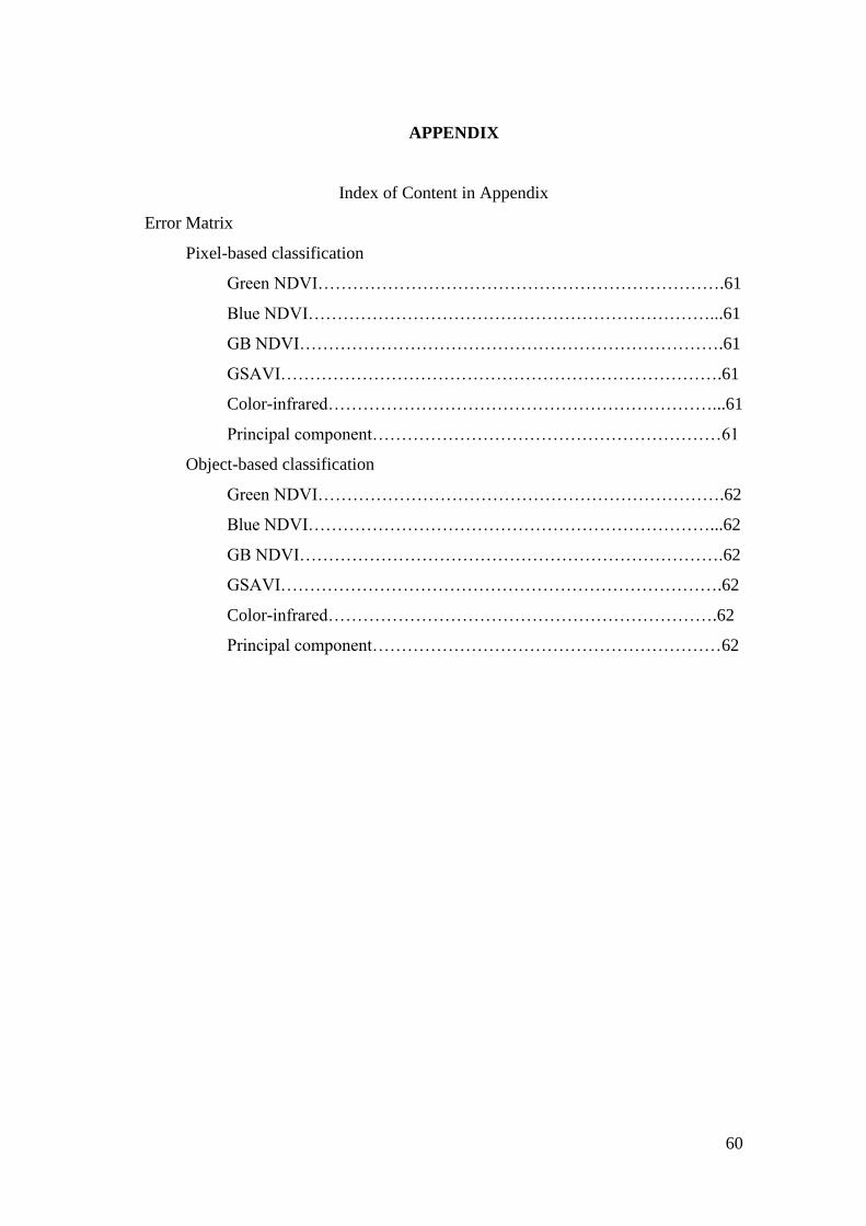
60

APPENDIX

Index of Content in Appendix

Error Matrix

Pixel-based classification

Green NDVI…………………………………………………………….61

Blue NDVI……………………………………………………………...61

GB NDVI……………………………………………………………….61

GSAVI………………………………………………………………….61

Color-infrared…………………………………………………………...61

Principal component……………………………………………………61

Object-based classification

Green NDVI…………………………………………………………….62

Blue NDVI……………………………………………………………...62

GB NDVI……………………………………………………………….62

GSAVI………………………………………………………………….62

Color-infrared………………………………………………………….62

Principal component……………………………………………………62

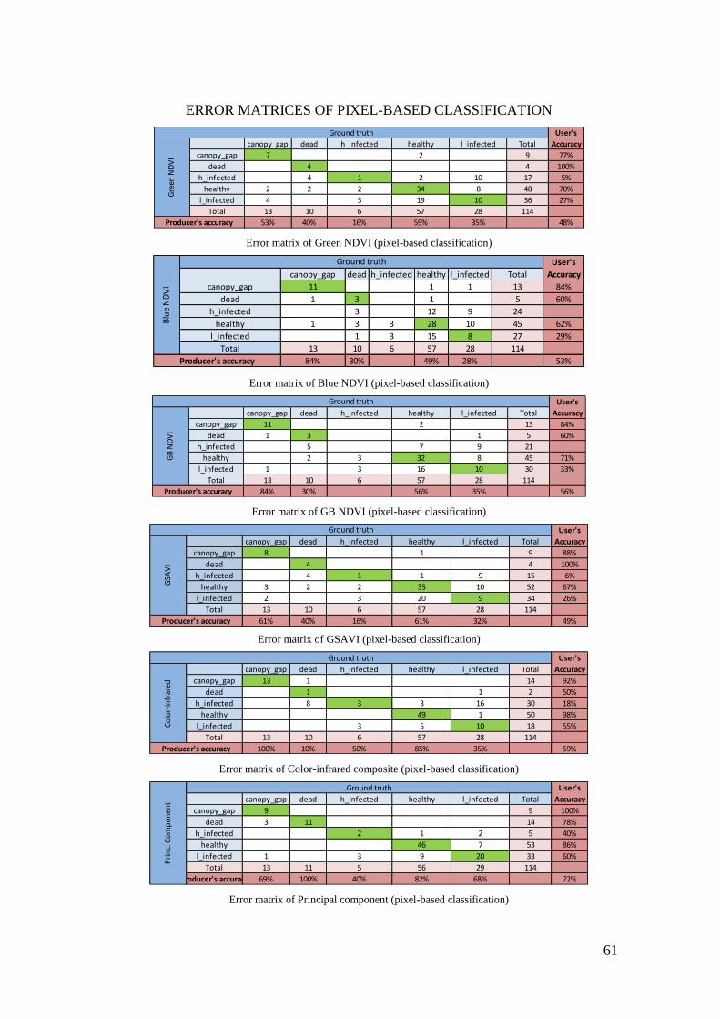
61

ERROR MATRICES OF PIXEL-BASED CLASSIFICATION

User's

canopy_gap dead h_infected healthy l_infected Total Accuracy

canopy_gap 7 2 9 77%

dead 4 4 100%

h_infected 4 1 2 10 17 5%

healthy 2 2 2 34 8 48 70%

l_infected 4 3 19 10 36 27%

Total 13 10 6 57 28 114

53% 40% 16% 59% 35% 48%Producer's accuracy

Ground truth

Gre

en N

DV

I

Error matrix of Green NDVI (pixel-based classification)

User's

canopy_gap dead h_infected healthy l_infected Total Accuracy

canopy_gap 11 1 1 13 84%

dead 1 3 1 5 60%

h_infected 3 12 9 24

healthy 1 3 3 28 10 45 62%

l_infected 1 3 15 8 27 29%

Total 13 10 6 57 28 114

84% 30% 49% 28% 53%

Blu

e N

DV

I

Ground truth

Producer's accuracy

Error matrix of Blue NDVI (pixel-based classification)

User's

canopy_gap dead h_infected healthy l_infected Total Accuracy

canopy_gap 11 2 13 84%

dead 1 3 1 5 60%

h_infected 5 7 9 21

healthy 2 3 32 8 45 71%

l_infected 1 3 16 10 30 33%

Total 13 10 6 57 28 114

84% 30% 56% 35% 56%

Ground truth

GB

ND

VI

Producer's accuracy

Error matrix of GB NDVI (pixel-based classification)

User's

canopy_gap dead h_infected healthy l_infected Total Accuracy

canopy_gap 8 1 9 88%

dead 4 4 100%

h_infected 4 1 1 9 15 6%

healthy 3 2 2 35 10 52 67%

l_infected 2 3 20 9 34 26%

Total 13 10 6 57 28 114

61% 40% 16% 61% 32% 49%

Ground truth

GSA

VI

Producer's accuracy

Error matrix of GSAVI (pixel-based classification)

User's

canopy_gap dead h_infected healthy l_infected Total Accuracy

canopy_gap 13 1 14 92%

dead 1 1 2 50%

h_infected 8 3 3 16 30 18%

healthy 49 1 50 98%

l_infected 3 5 10 18 55%

Total 13 10 6 57 28 114

100% 10% 50% 85% 35% 59%

Co

lor-

infr

ared

Producer's accuracy

Ground truth

Error matrix of Color-infrared composite (pixel-based classification)

User's

canopy_gap dead h_infected healthy l_infected Total Accuracy

canopy_gap 9 9 100%

dead 3 11 14 78%

h_infected 2 1 2 5 40%

healthy 46 7 53 86%

l_infected 1 3 9 20 33 60%

Total 13 11 5 56 29 114

Producer's accuracy 69% 100% 40% 82% 68% 72%

Pri

nc.

Co

mp

on

ent

Ground truth

Error matrix of Principal component (pixel-based classification)

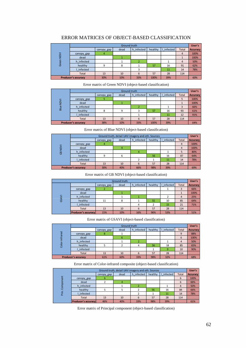
62

ERROR MATRICES OF OBJECT-BASED CLASSIFICATION

User's

canopy_gap dead h_infected healthy l_infected Total Accuracy

canopy_gap 4 4 100%

dead 1 1 100%

h_infected 1 2 1 4 50%

healthy 9 8 1 57 16 91 62%

l_infected 3 11 14 78%

Total 13 10 6 57 28 114

30% 10% 33% 100% 39% 60%

Gre

en N

DV

I

Ground truth

Producer's accuracy

Error matrix of Green NDVI (object-based classification)

User's

canopy_gap dead h_infected healthy l_infected Total Accuracy

canopy_gap 5 5 100%

dead 1 1 100%

h_infected 2 1 3 66%

healthy 8 9 3 57 16 93 61%

l_infected 1 11 12 91%

Total 13 10 6 57 28 114

38% 10% 33% 100% 39% 64%Producer's accuracy

Blu

e N

DV

I

Ground truth

Error matrix of Blue NDVI (object-based classification)

User's

canopy_gap dead h_infected healthy l_infected Total Accuracy

canopy_gap 4 4 100%

dead 4 4 100%

h_infected 4 1 5 80%

healthy 9 6 56 16 87 64%

l_infected 2 1 11 14 78%

Total 13 10 6 57 28 114

30% 40% 66% 98% 39% 69%

GB

ND

VI

Ground truth, detail UAV imagery and oth. Sources

Producer's accuracy

Error matrix of GB NDVI (object-based classification)

User's

canopy_gap dead h_infected healthy l_infected Total Accuracy

canopy_gap 2 1 3 66%

dead 1 1 100%

h_infected 1 1 2 4 25%

healthy 11 8 1 55 10 85 64%

l_infected 4 2 15 21 71%

Total 13 10 6 57 28 114

Producer's accuracy 15% 10% 16% 96% 53% 51%

Ground truth

GSA

VI

Error matrix of GSAVI (object-based classification)

User's

canopy_gap dead h_infected healthy l_infected Total Accuracy

canopy_gap 8 1 9 88%

dead 6 6 100%

h_infected 1 2 1 4 50%

healthy 5 2 4 56 18 85 65%

l_infected 1 9 10 90%

Total 13 10 6 57 28 114

61% 60% 33% 98% 32% 68%Producer's accuracy

Co

lor-

infr

ared

Ground truth

Error matrix of Color-infrared composite (object-based classification)

User's

canopy_gap dead h_infected healthy l_infected Total Accuracy

canopy_gap 6 6 100%

dead 2 4 6 66%

h_infected 1 2 1 4 50%

healthy 5 5 2 56 16 84 66%

l_infected 2 1 11 14 78%

Total 13 10 6 57 28 114

Producer's accuracy 46% 40% 33% 98% 39% 61%

Pri

n. C

om

po

nen

t

Ground truth, detail UAV imagery and oth. Sources

Error matrix of Principal component (object-based classification)