Geophysical Characterization Of A Cover With Capillary ... · With Capillary BarrierWith Capillary...
21
1/21 AGU 2007 _Acapulco May 22- 25 Geophysical Characterization Of A Cover Geophysical Characterization Of A Cover Geophysical Characterization Of A Cover Geophysical Characterization Of A Cover With Capillary Barrier With Capillary Barrier With Capillary Barrier With Capillary Barrier Effect Effect Effect Effect Chouteau, M . Chouteau, M . Chouteau, M . Chouteau, M . 1 1 1 , , , , Anterrieu, O. Anterrieu, O. Anterrieu, O. Anterrieu, O. 1, 1, 1, 1, Aubertin, Aubertin, Aubertin, Aubertin, M. M. M. M. 1 1 1 , , , Bussi Bussi Bussi Bussiè è ère re re re, , , B. B. B. B. 2, 2, 2, 2, & & & & Maqsoud Maqsoud Maqsoud Maqsoud, A. , A. , A. , A. 2 2 2 1 École Polytechnique, Montréal, Qc, Canada 2 UQAT, Rouyn-Noranda, Qc, Canada Industrial NSERC Polytechnique-UQAT Chair In Environment and Mine Waste Management
Transcript of Geophysical Characterization Of A Cover With Capillary ... · With Capillary BarrierWith Capillary...

1/21
AGU 2007 _Acapulco May 22- 25
Geophysical Characterization Of A Cover Geophysical Characterization Of A Cover Geophysical Characterization Of A Cover Geophysical Characterization Of A Cover With Capillary BarrierWith Capillary BarrierWith Capillary BarrierWith Capillary Barrier EffectEffectEffectEffect
Chouteau, M .Chouteau, M .Chouteau, M .Chouteau, M .1111, , , , Anterrieu, O.Anterrieu, O.Anterrieu, O.Anterrieu, O.1,1,1,1, Aubertin,Aubertin,Aubertin,Aubertin,M. M. M. M. 1111,,,, BussiBussiBussiBussièèèèrererere,,,, B.B.B.B.2,2,2,2, & & & & MaqsoudMaqsoudMaqsoudMaqsoud, A., A., A., A.2222
1École Polytechnique, Montréal, Qc, Canada2UQAT, Rouyn-Noranda, Qc, Canada
Industrial NSERC Polytechnique-UQAT ChairIn Environment and Mine Waste Management

2/21
The Problem
• Covers with Capillary Barrier Effect (CCBE) are used in mine environment & remediation to prevent oxygen flux to reachreactive mine tailings.
• Efficiency depends on water saturation. Suction breaks are constructed when needed to maintain saturation.
• Saturation must be monitored over very large areas (from 0.1km2
to 10km2) by mining compagnies
• Can geophysical techniques provide economic way to monitor saturation with some accuracy?

3/21
What is a CCBE?
capillary barrier principle: When a fine grained material overlies a coarser one, the water retention contrast between the two materials limits the vertical flow of water at the interface.
In the mining industry, a CCBE can be used to reduce the availability of oxygen to the underlying sulphidictailings
slope influences water movement in inclined covers
moisture distribution in the water retention layer is not uniform alongthe slope.
Under specific conditions, progressive desaturation is observed whenapproaching the top of the slope.

4/21
Suction break to control desaturation
slope effect can be reduced by creating a suction break
creation of a localized saturation area in the moisture-retentionlayer (i.e. zero suction).
The influenced zone shows lower suction and thus a higherdegree of saturation and lowergas diffusion characteristics.
GCL: geosynthetic clay liner with a low ksat

5/21
Saturation & Suction Break (SB): Numerical modeling results
•• Slope 3:1, L = 50 m, Moisture retaining layer: MRNSlope 3:1, L = 50 m, Moisture retaining layer: MRN --tailingstailings
0.75
0.80
0.85
0.90
0.95
1.00
0 10 20 30 40 50
Distance along the slope
Sat
ura
tion
ra
tio
7 days 15 days 30 days 60 days
HB-1
Toe Top
0.75
0.80
0.85
0.90
0.95
1.00
0 10 20 30 40 50
Distance along the slope
Sat
urat
ion
ratio
7 days 15 days 30 days 60 days
HB-2
Toe Top
0.75
0.80
0.85
0.90
0.95
1.00
0 10 20 30 40 50
Distance along the slopeS
atu
ratio
n r
atio
7 days 15 days 30 days 60 days
HB-3
Toe Top
Without SBWithout SB
With SBWith SB

6/21
LTA tailings impoundment; cover installed upon closure in 1996, using MRN tailings
Sand & gravel
Silt (non-reactivetailings)
Sand

7/21
Quick test (2005): Estimation of physical parameters
450 MHz
900 MHz
GPR 2D RI

8/21
Estimate of the fluid resistivity in the CCBE
Layer 1 : ρC1~ 400 Ω.m ; φ = 0.36 ; S = 0.4 ;
Archie’s law : ===> ρw= 8.3 Ω.m
Resistivity in the water retention layer
Layer 2 : φ = 0.44 ; ρc2 ~ 20 Ω.m
Schön,1996 : ===> σsurface = 26 mS/m
Formation factor
Resistivities of the CCBE layers
0.75
0.80
0.85
0.90
0.95
1.00
0 10 20 30 40 50
Distance along the slope
Sat
urat
ion
ratio
7 days 15 days 30 days 60 days
HB-1
Toe Top
Evolution of saturation in the water retention layer (Bussière et al., 2000)
)(surfaceF
weff σσσ +=
Smn
wc−−= ϕρρ .1
Smn
F−−
=ϕ

9/21
8608608608600.30.30.30.30.310.310.310.31Mine tailings (layer 4)Mine tailings (layer 4)Mine tailings (layer 4)Mine tailings (layer 4)
4004004004000.40.40.40.40.360.360.360.36sand (layer 3)sand (layer 3)sand (layer 3)sand (layer 3)
2929292927.727.727.727.725.825.825.825.820202020
0.83 [200.83 [200.83 [200.83 [20----30m] top 30m] top 30m] top 30m] top 0.85 [100.85 [100.85 [100.85 [10----20m]20m]20m]20m]0.88 [50.88 [50.88 [50.88 [5----10m]10m]10m]10m]1 [01 [01 [01 [0----5m] base5m] base5m] base5m] base
0.440.440.440.44SiltySiltySiltySilty material (layer 2)material (layer 2)material (layer 2)material (layer 2)
4004004004000.40.40.40.40.360.360.360.36Sand (layer 1)Sand (layer 1)Sand (layer 1)Sand (layer 1)
Estimated Estimated Estimated Estimated resistivityresistivityresistivityresistivityρ ( ( ( ( Ω.m ).m ).m ).m )Saturation Saturation Saturation Saturation
S S S S PorosityPorosityPorosityPorosity
φLayerLayerLayerLayer
Hydrogeological properties and resistivities of CCBE layers

10/21
Resistivity model (CCBE without succion break)
use of Res2Dmod & Res2Dinv
dipole-dipole array; 0.3 m minimum electrode spacing
Resistivity Modelling& Imaging

11/21
Inverted modelled data
0
-1
1
2
3
4
5
6
7
8
9
5 10 20 40 78 155 309 resistivity (Ω.m) 614
Resistivity imaging of a dipping CCBE depth of investigation : 1.5 m
discrimation of the 3 layers
evidence of saturated zones

12/21
CCBE with succion break
Succion break at 10 m from bottom of CCBE (Bussière et al., 2000)
0.75
0.80
0.85
0.90
0.95
1.00
0 10 20 30 40 50
Distance along the slope
Sat
urat
ion
ratio
7 days 15 days 30 days 60 days
HB-2
Toe Top
succion break

13/21
CCBE with succion break
discrimation of the 3 layers
evidence of saturated zones
• succion break
• Base of the CCBE
0
-1
1
2
3
4
5
6
7
8
9
5 10 40 78 155 309 resistivity (Ω.m)61420
Resistivity imaging of a CCBE with succion break

14/21
(Alharthi et al., 1987)( ) kkkk airwatermatrixmediumSS 2
12
12
1.2
1).1(..1 −++−= φφφ
0.1030.1030.1030.1030.00120.00120.00120.00128.58.58.58.55.55.55.55.50.30.30.30.3Mine Mine Mine Mine tailingstailingstailingstailings
(# 4)(# 4)(# 4)(# 4)
5.65.65.65.60.1050.1050.1050.1050.00250.00250.00250.00258.28.28.28.24.54.54.54.50.40.40.40.4Sand (# 3)Sand (# 3)Sand (# 3)Sand (# 3)
21.921.921.921.9
22.5322.5322.5322.53
23.523.523.523.5
28.0728.0728.0728.07
0.0730.0730.0730.073
0.0710.0710.0710.071
0.0680.0680.0680.068
0.0570.0570.0570.057
0.0340.0340.0340.034
0.0360.0360.0360.036
0.0390.0390.0390.039
0.050.050.050.05
16.7 top16.7 top16.7 top16.7 top
17.8 17.8 17.8 17.8
19.419.419.419.4
27.227.227.227.2 basebasebasebase
5.55.55.55.5
0.83 [200.83 [200.83 [200.83 [20----30] top30] top30] top30] top
0.85 [100.85 [100.85 [100.85 [10----20m]20m]20m]20m]
0.88 [50.88 [50.88 [50.88 [5----10m]10m]10m]10m]
1 [01 [01 [01 [0----5m] base5m] base5m] base5m] base
SiltySiltySiltySilty materialmaterialmaterialmaterial
(# 2)(# 2)(# 2)(# 2)
5.75.75.75.70,1050,1050,1050,1050.00250.00250.00250.00258.28.28.28.24.54.54.54.50.40.40.40.4Sand (# 1)Sand (# 1)Sand (# 1)Sand (# 1)
TWTTWTTWTTWT
(ns)(ns)(ns)(ns)
EM EM EM EM velocityvelocityvelocityvelocity
(m/ns)(m/ns)(m/ns)(m/ns)
ElectricalElectricalElectricalElectricalconductivityconductivityconductivityconductivity
( S/m)( S/m)( S/m)( S/m)
DielDielDielDiel. . . . ConstConstConstConst. . . . mediummediummediummedium
(K)(K)(K)(K)
DielDielDielDiel. . . . ConstConstConstConst. . . . matrixmatrixmatrixmatrix
saturationsaturationsaturationsaturation
( S )( S )( S )( S )LayerLayerLayerLayer
2D numerical GPR modelling

15/21
Discrimination of the 3 interfaces
Increasing TWT with saturation
Ambiguity in determining saturation if velocity or th ickness unknown
Modelled GPR response (450 MHz)
ModelModelModelModel
(GPRmax2D)
sandw. ret. layer
sand (drainage)
Mine tailings
K=27.2 K=19.4 K=17.8 K=16.7R1
R2
R3
R1
R2
R3
K=8.2
K=8.2
K=8.5
ResponseResponseResponseResponse
16/21
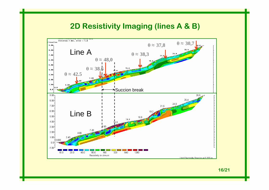
2D Resistivity Imaging (lines A & B)
Line A
Line B
Succion break
θ ≈ 42.5θ ≈ 38.6
θ ≈ 48,0θ ≈ 38,3
θ ≈ 30,7θ ≈ 37,8

17/21
2D Resistivity Imaging (lines A & C)
Line A
Line C
Succion break
(Away from SB)

18/21
R1 about 8 ns :
interface 1-2
R2about 28 ns :
interface 2-3
R3 about 36 ns :
interface 3-4
GPR reflection profiling at LTA (200 MHz)
Line B (200 Mhz)
R1 ≈ 9 ns
R3 ≈ 36 ns R2 ≈ 28 ns
Line A (200 Mhz)
R1 ≈ 8 ns
R2 ≈ 28 ns
θ ≈ 38.6
θ ≈ 42.5
θ ≈ 38.3θ ≈ 37.8
θ ≈ 48.0

19/21
R1 about 8 ns :
interface 1-2
R2about 28-32 ns :
interface 2-3
R3 (interface 3-4): not detected
High attenuationnear the toe
GPR reflection profiling at LTA (450 MHz)
Line A (450 Mhz)
R1≈ 8 ns
R2 ≈ 28 ns
Line B (450 Mhz)
R1 ≈ 8 ns
R2 ≈ 32 ns

20/21
Discussion• Imaging modelled resistivity data :
• excellent delineation of the 3 CCBE layers• sensitive to saturation variations in the w. retention layer
• Imaging modelled GPR reflection data :• excellent determination of interfaces between layers• TWT increases with saturation in w. retention layer
• Note: Results based on constant thickness homogeneous layers (0.3m, 0.8m, 0.5m)
• Survey resistivity data :– Show 1st layer thin (< 0.3 m) and heterogeneous; 2nd mapped as conductive with
variable thickness (average thickness agrees); 3rd mapped as resistive but lateralvariation.
– 2nd layer resistivities correlated with water content– No easy direct relation between resistivity and saturation– Problem of equivalence (?) knowing that thickness varies
• Survey GPR data:– Show good determination of the two first interfaces (1-2, 2-3); the 3rd is difficult
because of attenuation– Changes in TWT may reflect changes in saturation as well as changes in thickness.

21/21
Conclusion
• Both methods are sensitive to change in water saturation; relative changes but not absolute values of saturation may be tracktable. Alsoboth methods are sensitive to thickness variations in layer 2.
• Further work: – Need better estimation of 2nd layer σeff with σw and σsurf; effect of
T(0C) on interpretation.– Cooperative/joint inversion of both data sets for resistivity,
thickness and velocity.– Use (inversion with constrains) TDR (and suction) data recorded on
sites at few places.– calibration pads on site (thickness and diel. const. known) and use
GPR reflectivity.– A combination of the solutions above.