Geometry of Optimization and Implicit Regularization in ... · GEOMETRY OF OPTIMIZATION AND...

GEOMETRY OF OPTIMIZATION AND IMPLICIT REGULARIZATION DEEP LEARNING

Geometry of Optimization and Implicit Regularizationin Deep Learning

This survey chapter was done as a part of Intel Collaborative Research institute for Computational Intelli-gence (ICRI-CI) “Why & When Deep Learning works – looking inside Deep Learning” compendium withthe generous support of ICRI-CI.

Behnam Neyshabur [email protected] Technological Institute at ChicagoChicago, IL 60637, USA

Ryota Tomioka [email protected] CambridgeCambridge, CB1 2FB, UK

Ruslan Salakhutdinov [email protected] of Computer ScienceCarnegie Mellon UniversityPittsburgh, PA 15213, USA

Nathan Srebro [email protected]

Toyota Technological Institute at ChicagoChicago, IL 60637, USA

Editor:

Abstract

We argue that the optimization plays a crucial role in generalization of deep learning modelsthrough implicit regularization. We do this by demonstrating that generalization ability is notcontrolled by network size but rather by some other implicit control. We then demonstrate howchanging the empirical optimization procedure can improve generalization, even if actual opti-mization quality is not affected. We do so by studying the geometry of the parameter space of deepnetworks, and devising an optimization algorithm attuned to this geometry.

Keywords: Deep Learning, Implicit Regularization, Geometry of Optimization, Path-norm, Path-SGD

1. Introduction

Central to any form of learning is an inductive bias that induces some sort of capacity control(i.e. restricts or encourages predictors to be “simple” in some way), which in turn allows for gen-eralization. The success of learning then depends on how well the inductive bias captures reality(i.e. how expressive is the hypothesis class of “simple” predictors) relative to the capacity induced,as well as on the computational complexity of fitting a “simple” predictor to the training data.

1

arX

iv:1

705.

0307

1v1

[cs

.LG

] 8

May

201

7

NEYSHABUR ET AL.

Let us consider learning with feed-forward networks from this perspective. If we search for theweights minimizing the training error, we are essentially considering the hypothesis class of predic-tors representable with different weight vectors, typically for some fixed architecture. Capacity isthen controlled by the size (number of weights) of the network1. Our justification for using such net-works is then that many interesting and realistic functions can be represented by not-too-large (andhence bounded capacity) feed-forward networks. Indeed, in many cases we can show how specificarchitectures can capture desired behaviors. More broadly, any O(T ) time computable function canbe captured by an O(T 2) sized network, and so the expressive power of such networks is indeedgreat (Sipser, 2006, Theorem 9.25).

At the same time, we also know that learning even moderately sized networks is computationallyintractable—not only is it NP-hard to minimize the empirical error, even with only three hiddenunits, but it is hard to learn small feed-forward networks using any learning method (subject tocryptographic assumptions). That is, even for binary classification using a network with a singlehidden layer and a logarithmic (in the input size) number of hidden units, and even if we know thetrue targets are exactly captured by such a small network, there is likely no efficient algorithm thatcan ensure error better than 1/2 (Sherstov, 2006; Daniely et al., 2014)—not if the algorithm triesto fit such a network, not even if it tries to fit a much larger network, and in fact no matter howthe algorithm represents predictors. And so, merely knowing that some not-too-large architecture isexcellent in expressing reality does not explain why we are able to learn using it, nor using an evenlarger network. Why is it then that we succeed in learning using multilayer feed-forward networks?Can we identify a property that makes them possible to learn? An alternative inductive bias?

In section 2, we make our first steps at shedding light on this question by going back to ourunderstanding of network size as the capacity control at play. Our main observation, based onempirical experimentation with single-hidden-layer networks of increasing size (increasing numberof hidden units), is that size does not behave as a capacity control parameter, and in fact there mustbe some other, implicit, capacity control at play. We suggest that this hidden capacity control mightbe the real inductive bias when learning with deep networks.

Revisiting the choice of gradient descent, we recall that optimization is inherently tied to achoice of geometry or measure of distance, norm or divergence. Gradient descent for example istied to the `2 norm as it is the steepest descent with respect to `2 norm in the parameter space, whilecoordinate descent corresponds to steepest descent with respect to the `1 norm and exp-gradient(multiplicative weight) updates is tied to an entropic divergence. Moreover, at least when the ob-jective function is convex, convergence behavior is tied to the corresponding norms or potentials.For example, with gradient descent, or SGD, convergence speeds depend on the `2 norm of theoptimum. The norm or divergence can be viewed as a regularizer for the updates. There is thereforealso a strong link between regularization for optimization and regularization for learning: opti-mization may provide implicit regularization in terms of its corresponding geometry, and for idealoptimization performance the optimization geometry should be aligned with inductive bias drivingthe learning (Srebro et al., 2011).

Is the `2 geometry on the weights the appropriate geometry for the space of deep networks? Orcan we suggest a geometry with more desirable properties that would enable faster optimization and

1. The exact correspondence depends on the activation function—for hard thresholding activation the pseudo-dimension, and hence sample complexity, scales as O(S logS), where S is the number of weights in the network.With sigmoidal activation it is between Ω(S2) and O(S4) (Anthony and Bartlett, 1999).

2


perhaps also better implicit regularization? As suggested above, this question is also linked to thechoice of an appropriate regularizer for deep networks.

Focusing on networks with RELU activations in this section, we observe that scaling down theincoming edges to a hidden unit and scaling up the outgoing edges by the same factor yields anequivalent network computing the same function. Since predictions are invariant to such rescalings,it is natural to seek a geometry, and corresponding optimization method, that is similarly invariant.

We consider here a geometry inspired by max-norm regularization (regularizing the maximumnorm of incoming weights into any unit) which seems to provide a better inductive bias comparedto the `2 norm (weight decay) (Goodfellow et al., 2013; Srivastava et al., 2014). But to achieverescaling invariance, we use not the max-norm itself, but rather the minimum max-norm over allrescalings of the weights. We discuss how this measure can be expressed as a “path regularizer”and can be computed efficiently.

We therefore suggest a novel optimization method, Path-SGD, that is an approximate steep-est descent method with respect to path regularization. Path-SGD is rescaling-invariant and wedemonstrate that Path-SGD outperforms gradient descent and AdaGrad for classifications tasks onseveral benchmark datasets. This again demonstrates the importance of implicit regularization thatis introduced by optimization.

This summary paper combines material previously presented by the authors at the 3rd Interna-tional Conference on Learning Representations (ICLR), the 28th Conference on Learning Theory(COLT) and Advances in Neural Information Processing Systems (NIPS) 28, as well as Intel Col-laborative Research Institutes retreats (Neyshabur et al., 2015a,b,c).

Notations A feedforward neural network that computes a function f : RD → RC can be repre-sented by a directed acyclic graph (DAG) G(V,E) with D input nodes vin[1], . . . , vin[D] ∈ V , Coutput nodes vout[1], . . . , vout[C] ∈ V , weights w : E → R and an activation function σ : R → Rthat is applied on the internal nodes (hidden units). We denote the function computed by thisnetwork as fG,w,σ. In this paper we focus on RELU (REctified Linear Unit) activation functionσRELU(x) = max0, x. We refer to the depth d of the network which is the length of the longestdirected path in G. For any 0 ≤ i ≤ d, we define V i

in to be the set of vertices with longest path oflength i to an input unit and V i

out is defined similarly for paths to output units. In layered networksV i

in = V d−iout is the set of hidden units in a hidden layer i.

2. Implicit Regularization

Consider training a feed-forward network by finding the weights minimizing the training error.Specifically, we will consider a network with D real-valued inputs x = (x[1], . . . , x[D]), a singlehidden layer withH rectified linear units, andC outputs y[1], . . . , y[k] where the weights are learnedby minimizing a (truncated) soft-max cross entropy loss2 on n labeled training examples. The totalnumber of weights is then H(C +D).

2. When using soft-max cross-entropy, the loss is never exactly zero for correct predictions with finite mar-gins/confidences. Instead, if the data is separable, in order to minimize the loss the weights need to be scaled uptoward infinity and the cross entropy loss goes to zero, and a global minimum is never attained. In order to be ableto say that we are actually reaching a zero loss solution, and hence a global minimum, we use a slightly modifiedsoft-max which does not noticeably change the results in practice. This truncated loss returns the same exact valuefor wrong predictions or correct prediction with confidences less than a threshold but returns zero for correct predic-tions with large enough margins: Let siki=1 be the scores for k possible labels and c be the correct labels. Thenthe soft-max cross-entropy loss can be written as `(s, c) = ln

∑i exp(si − sc) but we instead use the differentiable

3

NEYSHABUR ET AL.

4 8 16 32 64 128 256 512 1K 2K 4K0

0.01

0.02

0.03

0.04

0.05

0.06

0.07

0.08

0.09

0.1

H

Erro

r

TrainingTest (at convergence)Test (early stopping)

4 8 16 32 64 128 256 512 1K 2K 4K0

0.1

0.2

0.3

0.4

0.5

0.6

H

Erro

r

TrainingTest (at convergence)Test (early stopping)

MNIST CIFAR-10

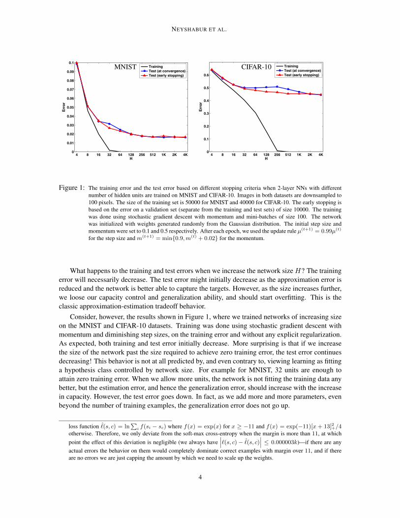
Figure 1: The training error and the test error based on different stopping criteria when 2-layer NNs with differentnumber of hidden units are trained on MNIST and CIFAR-10. Images in both datasets are downsampled to100 pixels. The size of the training set is 50000 for MNIST and 40000 for CIFAR-10. The early stopping isbased on the error on a validation set (separate from the training and test sets) of size 10000. The trainingwas done using stochastic gradient descent with momentum and mini-batches of size 100. The networkwas initialized with weights generated randomly from the Gaussian distribution. The initial step size andmomentum were set to 0.1 and 0.5 respectively. After each epoch, we used the update rule µ(t+1) = 0.99µ(t)

for the step size and m(t+1) = min0.9,m(t) + 0.02 for the momentum.

What happens to the training and test errors when we increase the network sizeH? The trainingerror will necessarily decrease. The test error might initially decrease as the approximation error isreduced and the network is better able to capture the targets. However, as the size increases further,we loose our capacity control and generalization ability, and should start overfitting. This is theclassic approximation-estimation tradeoff behavior.

Consider, however, the results shown in Figure 1, where we trained networks of increasing sizeon the MNIST and CIFAR-10 datasets. Training was done using stochastic gradient descent withmomentum and diminishing step sizes, on the training error and without any explicit regularization.As expected, both training and test error initially decrease. More surprising is that if we increasethe size of the network past the size required to achieve zero training error, the test error continuesdecreasing! This behavior is not at all predicted by, and even contrary to, viewing learning as fittinga hypothesis class controlled by network size. For example for MNIST, 32 units are enough toattain zero training error. When we allow more units, the network is not fitting the training data anybetter, but the estimation error, and hence the generalization error, should increase with the increasein capacity. However, the test error goes down. In fact, as we add more and more parameters, evenbeyond the number of training examples, the generalization error does not go up.

loss function ˆ(s, c) = ln∑

i f(si − sc) where f(x) = exp(x) for x ≥ −11 and f(x) = exp(−11)[x + 13]2+/4otherwise. Therefore, we only deviate from the soft-max cross-entropy when the margin is more than 11, at whichpoint the effect of this deviation is negligible (we always have

∣∣∣`(s, c)− ˆ(s, c)∣∣∣ ≤ 0.000003k)—if there are any

actual errors the behavior on them would completely dominate correct examples with margin over 11, and if thereare no errors we are just capping the amount by which we need to scale up the weights.

4


0 100 200 3000

0.5

1

1.5

2

2.5

Epoch

Obj

ectiv

e

BalancedUnbalanced

(a) Training on MNIST

100

10-4

SGD Update

100

~100

~104

~100

1

1 Rescaling

1

u

v

u

v

u

v

≈

(b) Weight explosion in an unbalanced network

8

68

37

78

4 vu6

11

14

21

1 vu60.2

10.570.1

10.230.4

20.570.1

30.1 vu60

100.1

100.4

200.1

0.1vu

SGD Update

SGD Update ≈Rescaling

(c) Poor updates in an unbalanced network

Figure 2: (a): Evolution of the cross-entropy error function when training a feed-forward network on MNIST with twohidden layers, each containing 4000 hidden units. The unbalanced initialization (blue curve) is generatedby applying a sequence of rescaling functions on the balanced initializations (red curve). (b): Updates for asimple case where the input is x = 1, thresholds are set to zero (constant), the stepsize is 1, and the gradientwith respect to output is δ = −1. (c): Updated network for the case where the input is x = (1, 1), thresholdsare set to zero (constant), the stepsize is 1, and the gradient with respect to output is δ = (−1,−1).

What is happening here? A possible explanation is that the optimization is introducing someimplicit regularization. That is, we are implicitly trying to find a solution with small “complexity”,for some notion of complexity, perhaps norm. This can explain why we do not overfit even whenthe number of parameters is huge. Furthermore, increasing the number of units might allow forsolutions that actually have lower “complexity”, and thus generalization better. Perhaps an idealthen would be an infinite network controlled only through this hidden complexity.

We want to emphasize that we are not including any explicit regularization, neither as an explicitpenalty term nor by modifying optimization through, e.g., drop-outs, weight decay, or with one-passstochastic methods. We are using a stochastic method, but we are running it to convergence—we achieve zero surrogate loss and zero training error. In fact, we also tried training using batchconjugate gradient descent and observed almost identical behavior. But it seems that even still, weare not getting to some random global minimum—indeed for large networks the vast majority ofthe many global minima of the training error would horribly overfit. Instead, the optimization isdirecting us toward a “low complexity” global minimum.

We have argued that the implicit regularization is due to the optimization. It is therefore ex-pected that different optimization methods introduce different implicit regularizations which leadsto different generalization properties. In an attempt to find an optimization method with better gen-eralization properties, we recall that the optimization is also tied to a choice of geometry/distancemeasure in the parameter space. We look into the desirable properties of a geometry for neuralnetworks and suggest an optimization algorithm that is tied to that geometry.

5

NEYSHABUR ET AL.

3. The Geometry of Optimization: Rescaling and Unbalanceness

In this section, we look at the behavior of the Euclidean geometry under rescaling and unbalance-ness. One of the special properties of RELU activation function is non-negative homogeneity. Thatis, for any scalar c ≥ 0 and any x ∈ R, we have σRELU(c · x) = c · σRELU(x). This interestingproperty allows the network to be rescaled without changing the function computed by the network.We define the rescaling function ρc,v(w), such that given the weights of the network w : E → R, aconstant c > 0, and a node v, the rescaling function multiplies the incoming edges and divides theoutgoing edges of v by c. That is, ρc,v(w) maps w to the weights w for the rescaled network, wherefor any (u1 → u2) ∈ E:

w(u1→u2) =

c.w(u1→u2) u2 = v,1cw(u1→u2) u1 = v,

w(u1→u2) otherwise.

(1)

It is easy to see that the rescaled network computes the same function, i.e. fG,w,σRELU = fG,ρc,v(w),σRELU.

We say that the two networks with weights w and w are rescaling equivalent denoted by w ∼ w ifand only if one of them can be transformed to another by applying a sequence of rescaling functionsρc,v.

Given a training set S = (x1, yn), . . . , (xn, yn), our goal is to minimize the following objec-tive function:

L(w) =1

n

n∑i=1

`(fw(xi), yi). (2)

Let w(t) be the weights at step t of the optimization. We consider update step of the following formw(t+1) = w(t) + ∆w(t+1). For example, for gradient descent, we have ∆w(t+1) = −η∇L(w(t)),where η is the step-size. In the stochastic setting, such as SGD or mini-batch gradient descent, wecalculate the gradient on a small subset of the training set.

Since rescaling equivalent networks compute the same function, it is desirable to have an updaterule that is not affected by rescaling. We call an optimization method rescaling invariant if theupdates of rescaling equivalent networks are rescaling equivalent. That is, if we start at either oneof the two rescaling equivalent weight vectors w(0) ∼ w(0), after applying t update steps separatelyon w(0) and w(0), they will remain rescaling equivalent and we have w(t) ∼ w(t).

Unfortunately, gradient descent is not rescaling invariant. The main problem with the gradientupdates is that scaling down the weights of an edge will also scale up the gradient which, as we seelater, is exactly the opposite of what is expected from a rescaling invariant update.

Furthermore, gradient descent performs very poorly on “unbalanced” networks. We say thata network is balanced if the norm of incoming weights to different units are roughly the same orwithin a small range. For example, Figure a shows a huge gap in the performance of SGD initializedwith a randomly generated balanced networkw(0), when training on MNIST, compared to a networkinitialized with unbalanced weights w(0). Here w(0) is generated by applying a sequence of randomrescaling functions on w(0) (and therefore w(0) ∼ w(0)).

In an unbalanced network, gradient descent updates could blow up the smaller weights, whilekeeping the larger weights almost unchanged. This is illustrated in Figure b. If this were the onlyissue, one could scale down all the weights after each update. However, in an unbalanced network,the relative changes in the weights are also very different compared to a balanced network. For

6


example, Figure c shows how two rescaling equivalent networks could end up computing a verydifferent function after only a single update.

4. Magnitude/Scale measures for deep networks

Following Neyshabur et al. (2015b), we consider the grouping of weights going into each nodeof the network. This forms the following generic group-norm type regularizer, parametrized by1 ≤ p, q ≤ ∞:

µp,q(w) =

∑v∈V

∑(u→v)∈E

∣∣w(u→v)∣∣pq/p

1/q

. (3)

Two simple cases of above group-norm are p = q = 1 and p = q = 2 that correspond to overall`1 regularization and weight decay respectively. Another form of regularization that is shown to bevery effective in RELU networks is the max-norm regularization, which is the maximum over allunits of norm of incoming edge to the unit3 (Goodfellow et al., 2013; Srivastava et al., 2014). Themax-norm correspond to “per-unit” regularization when we set q = ∞ in equation (4) and can bewritten in the following form:

µp,∞(w) = supv∈V

∑(u→v)∈E

∣∣w(u→v)∣∣p1/p

(4)

Weight decay is probably the most commonly used regularizer. On the other hand, per-unitregularization might not seem ideal as it is very extreme in the sense that the value of regularizercorresponds to the highest value among all nodes. However, the situation is very different fornetworks with RELU activations (and other activation functions with non-negative homogeneityproperty). In these cases, per-unit `2 regularization has shown to be very effective (Srivastava et al.,2014). The main reason could be because RELU networks can be rebalanced in such a way thatall hidden units have the same norm. Hence, per-unit regularization will not be a crude measureanymore.

Since µp,∞ is not rescaling invariant and the values of the scale measure are different for rescal-ing equivalent networks, it is desirable to look for the minimum value of a regularizer among allrescaling equivalent networks. Surprisingly, for a feed-forward network, the minimum `p per-unitregularizer among all rescaling equivalent networks can be efficiently computed by a single forwardstep. To see this, we consider the vector π(w), the path vector, where the number of coordinatesof π(w) is equal to the total number of paths from the input to output units and each coordinate ofπ(w) is the equal to the product of weights along a path from an input nodes to an output node. The`p-path regularizer is then defined as the `p norm of π(w) (Neyshabur et al., 2015b):

φp(w) = ‖π(w)‖p =

∑vin[i]

e1→v1e2→v2...

ed→vout[j]

∣∣∣∣∣d∏

k=1

wek

∣∣∣∣∣p

1/p

(5)

3. This definition of max-norm is a bit different than the one used in the context of matrix factorization (Srebro andShraibman, 2005). The later is similar to the minimum upper bound over `2 norm of both outgoing edges from theinput units and incoming edges to the output units in a two layer feed-forward network.

7

NEYSHABUR ET AL.

The following Lemma establishes that the `p-path regularizer corresponds to the minimum over allequivalent networks of the per-unit `p norm:

Lemma 4.1 (Neyshabur et al. (2015b)) φp(w) = minw∼w

(µp,∞(w)

)dThe definition (5) of the `p-path regularizer involves an exponential number of terms. But it canbe computed efficiently by dynamic programming in a single forward step using the followingequivalent form as nested sums:

φp(w) =

∑(vd−1→vout[j])∈E

∣∣w(vd−1→vout[j])

∣∣p ∑(vd−2→vd−1)∈E

· · ·∑

(vin[i]→v1)∈E

∣∣w(vin[i]→v1)∣∣p1/p

A straightforward consequence of Lemma 4.1 is that the `p path-regularizer φp is invariant to rescal-ing, i.e. for any w ∼ w, φp(w) = φp(w).

5. Path-SGD: An Approximate Path-Regularized Steepest Descent

Motivated by empirical performance of max-norm regularization and the fact that path-regularizeris invariant to rescaling, we are interested in deriving the steepest descent direction with respect tothe path regularizer φp(w):

w(t+1) = arg minw

η⟨∇L(w(t)), w

⟩+

1

2

∥∥∥π(w)− π(w(t))∥∥∥2p

(6)

= arg minw

η⟨∇L(w(t)), w

⟩+

∑vin[i]

e1→v1e2→v2...

ed→vout[j]

(d∏

k=1

wek −d∏

k=1

w(t)ek

)

)p2/p

= arg minwJ (t)(w)

The steepest descent step (6) is hard to calculate exactly. Instead, we will update each coordinatewe independently (and synchronously) based on (6). That is:

w(t+1)e = arg min

we

J (t)(w) s.t. ∀e′ 6=e we′ = w(t)e′ (7)

Taking the partial derivative with respect to we and setting it to zero we obtain:

0 = η∂L

∂we(w(t))−

(we − w(t)

e

) ∑vin[i]···

e→...vout[j]

∏ek 6=e

∣∣∣w(t)e

∣∣∣p

2/p

where vin[i] · · · e→ . . . vout[j] denotes the paths from any input unit i to any output unit j that includese. Solving for we gives us the following update rule:

w(t+1)e = w(t)

e −η

γp(w(t), e)

∂L

∂w(w(t)) (8)

8


where γp(w, e) is given as

γp(w, e) =

∑vin[i]···

e→...vout[j]

∏ek 6=e|wek |

p

2/p

(9)

We call the optimization using the update rule (8) path-normalized gradient descent. When used instochastic settings, we refer to it as Path-SGD.

Now that we know Path-SGD is an approximate steepest descent with respect to the path-regularizer, we can ask whether or not this makes Path-SGD a rescaling invariant optimizationmethod. The next theorem proves that Path-SGD is indeed rescaling invariant.

Theorem 5.1 Path-SGD is rescaling invariant.

Proof It is sufficient to prove that using the update rule (8), for any c > 0 and any v ∈ E, ifw(t) = ρc,v(w

(t)), then w(t+1) = ρc,v(w(t+1)). For any edge e in the network, if e is neither

incoming nor outgoing edge of the node v, then w(e) = w(e), and since the gradient is also thesame for edge e we have w(t+1)

e = w(t+1)e . However, if e is an incoming edge to v, we have that

w(t)(e) = cw(t)(e). Moreover, since the outgoing edges of v are divided by c, we get γp(w(t), e) =γp(w(t),e)

c2and ∂L

∂we(w(t)) = ∂L

c∂we(w(t)). Therefore,

w(t+1)e = cw(t)

e −c2η

γp(w(t), e)

∂L

c∂we(w(t))

= c

(w(t) − η

γp(w(t), e)

∂L

∂we(w(t))

)= cw(t+1)

e .

A similar argument proves the invariance of Path-SGD update rule for outgoing edges of v. There-fore, Path-SGD is rescaling invariant.

Efficient Implementation: The Path-SGD update rule (8), in the way it is written, needs to con-sider all the paths, which is exponential in the depth of the network. However, it can be calculatedin a time that is no more than a forward-backward step on a single data point. That is, in a mini-batch setting with batch size B, if the backpropagation on the mini-batch can be done in time BT ,the running time of the Path-SGD on the mini-batch will be roughly (B + 1)T – a very moderateruntime increase with typical mini-batch sizes of hundreds or thousands of points. Algorithm 1shows an efficient implementation of the Path-SGD update rule.

We next compare Path-SGD to other optimization methods in both balanced and unbalancedsettings.

6. Experiments on Path-SGD

We compare `2-Path-SGD to two commonly used optimization methods in deep learning, SGDand AdaGrad. We conduct our experiments on four common benchmark datasets: the standardMNIST dataset of handwritten digits (LeCun et al., 1998); CIFAR-10 and CIFAR-100 datasets

9

NEYSHABUR ET AL.

Algorithm 1 Path-SGD update rule

1: ∀v∈V 0inγin(v) = 1 . Initialization

2: ∀v∈V 0outγout(v) = 1

3: for i = 1 to d do4: ∀v∈V i

inγin(v) =

∑(u→v)∈E γin(u)

∣∣w(u,v)

∣∣p5: ∀v∈V i

outγout(v) =

∑(v→u)∈E

∣∣w(v,u)

∣∣p γout(u)6: end for7: ∀(u→v)∈E γ(w(t), (u, v)) = γin(u)2/pγout(v)2/p

8: ∀e∈Ew(t+1)e = w

(t)e − η

γ(w(t),e)∂L∂we

(w(t)) . Update Rule

Table 1: General information on datasets used in the experiments on feedforward networks.Data Set Dimensionality Classes Training Set Test Set

CIFAR-10 3072 (32× 32 color) 10 50000 10000CIFAR-100 3072 (32× 32 color) 100 50000 10000

MNIST 784 (28× 28 grayscale) 10 60000 10000SVHN 3072 (32× 32 color) 10 73257 26032

of tiny images of natural scenes (Krizhevsky and Hinton, 2009); and Street View House Numbers(SVHN) dataset containing color images of house numbers collected by Google Street View (Netzeret al., 2011). Details of the datasets are shown in Table 1.

In all of our experiments, we trained feed-forward networks with two hidden layers, each con-taining 4000 hidden units. We used mini-batches of size 100 and the step-size of 10−α, where αis an integer between 0 and 10. To choose α, for each dataset, we considered the validation errorsover the validation set (10000 randomly chosen points that are kept out during the initial training)and picked the one that reaches the minimum error faster. We then trained the network over theentire training set. All the networks were trained both with and without dropout. When trainingwith dropout, at each update step, we retained each unit with probability 0.5.

The optimization results are shown in Figure 3. For each of the four datasets, the plots forobjective function (cross-entropy), the training error and the test error are shown from left to rightwhere in each plot the values are reported on different epochs during the optimization. The dropoutis used for the experiments on CIFAR-100 and SVHN. Please see Neyshabur et al. (2015a) for amore complete set of experimental results.

We can see in Figure 3 that not only does Path-SGD often get to the same value of objectivefunction, training and test error faster, but also the plots for test errors demonstrate that implicit regu-larization due to steepest descent with respect to path-regularizer leads to a solution that generalizesbetter. This provides further evidence on the role of implicit regularization in deep learning.

The results suggest that Path-SGD outperforms SGD and AdaGrad in two different ways. First,it can achieve the same accuracy much faster and second, the implicit regularization by Path-SGDleads to a local minima that can generalize better even when the training error is zero. This canbe better analyzed by looking at the plots for more number of epochs which we have providedin Neyshabur et al. (2015a). We should also point that Path-SGD can be easily combined with

10


0 20 40 60 80 1000

0.5

1

1.5

2

2.5.

0 20 40 60 80 1000

0.5

1

1.5

2

2.5

.

0 20 40 60 80 1000

1

2

3

4

5

.

0 20 40 60 80 1000

0.5

1

1.5

2

2.5

Epoch

.

0 20 40 60 80 1000

0.05

0.1

0.15

0.2

.

0 20 40 60 80 1000

0.005

0.01

0.015

0.02

.

0 20 40 60 80 1000

0.2

0.4

0.6

0.8

.

0 20 40 60 80 1000

0.1

0.2

0.3

0.4

Epoch

.

0 20 40 60 80 1000.4

0.45

0.5

0.55

0.6

.

Path−SGD − UnbalancedSGD − BalancedSGD − UnbalancedAdaGrad − BalancedAdaGrad − Unbalanced

0 20 40 60 80 1000.015

0.02

0.025

0.03

0.035

.

0 20 40 60 80 1000.6

0.65

0.7

0.75

0.8

.

0 20 40 60 80 1000.12

0.13

0.14

0.15

0.16

0.17

0.18

Epoch

.

CIF

AR

-10

MN

IST

CIF

AR

100

SVH

NCross-Entropy Training Loss 0/1 Training Error 0/1 Test Error

Figure 3: Learning curves using different optimization methods for 4 datasets without dropout. Left panel displaysthe cross-entropy objective function; middle and right panels show the corresponding values of the trainingand test errors, where the values are reported on different epochs during the course of optimization.We triedboth balanced and unbalanced initializations. In balanced initialization, incoming weights to each unit vare initialized to i.i.d samples from a Gaussian distribution with standard deviation 1/

√fan-in(v). In the

unbalanced setting, we first initialized the weights to be the same as the balanced weights. We then picked2000 hidden units randomly with replacement. For each unit, we multiplied its incoming edge and divided itsoutgoing edge by 10c, where c was chosen randomly from log-normal distribution. Although we proved thatPath-SGD updates are the same for balanced and unbalanced initializations, to verify that despite numericalissues they are indeed identical, we trained Path-SGD with both balanced and unbalanced initializations.Since the curves were exactly the same we only show a single curve. Best viewed in color.

AdaGrad or Adam to take advantage of the adaptive stepsize or used together with a momentumterm. This could potentially perform even better compare to Path-SGD.

11

NEYSHABUR ET AL.

7. Discussion

We demonstrated the implicit regularization in deep learning through experiments and discussedthe importance of geometry of optimization in finding a “low complexity” solution. Based on that,we revisited the choice of the Euclidean geometry on the weights of RELU networks, suggested analternative optimization method approximately corresponding to a different geometry, and showedthat using such an alternative geometry can be beneficial. In this work we show proof-of-conceptsuccess, and we expect Path-SGD to be beneficial also in large-scale training for very deep convolu-tional networks. Combining Path-SGD with AdaGrad, with momentum or with other optimizationheuristics might further enhance results.

Although we do believe Path-SGD is a very good optimization method, and is an easy plug-in forSGD, we hope this work will also inspire others to consider other geometries, other regularizers andperhaps better, update rules. A particular property of Path-SGD is its rescaling invariance, which weargue is appropriate for RELU networks. But Path-SGD is certainly not the only rescaling invariantupdate possible, and other invariant geometries might be even better.

Finally, we choose to use steepest descent because of its simplicity of implementation. A bet-ter choice might be mirror descent with respect to an appropriate potential function, but such aconstruction seems particularly challenging considering the non-convexity of neural networks.

Acknowledgments

Research was partially funded by NSF award IIS-1302662 and Intel ICRI-CI.

References

Martin Anthony and Peter L Bartlett. Neural network learning: Theoretical foundations. CambridgeUniversity Press, 1999.

Amit Daniely, Nati Linial, and Shai Shalev-Shwartz. From average case complexity to improperlearning complexity. STOC, 2014.

Ian J. Goodfellow, David Warde-Farley, Mehdi Mirza, Aaron C. Courville, and Yoshua Bengio.Maxout networks. In Proceedings of the 30th International Conference on Machine Learning,ICML, pages 1319–1327, 2013.

Alex Krizhevsky and Geoffrey Hinton. Learning multiple layers of features from tiny images.Computer Science Department, University of Toronto, Tech. Rep, 1(4):7, 2009.

Yann LeCun, Leon Bottou, Yoshua Bengio, and Patrick Haffner. Gradient-based learning appliedto document recognition. Proceedings of the IEEE, 86(11):2278–2324, 1998.

Yuval Netzer, Tao Wang, Adam Coates, Alessandro Bissacco, Bo Wu, and Andrew Y Ng. Readingdigits in natural images with unsupervised feature learning. In NIPS workshop on deep learningand unsupervised feature learning, 2011.

Behnam Neyshabur, Ruslan R Salakhutdinov, and Nati Srebro. Path-sgd: Path-normalized opti-mization in deep neural networks. In Advances in Neural Information Processing Systems, pages2413–2421, 2015a.

12


Behnam Neyshabur, Ryota Tomioka, and Nathan Srebro. Norm-based capacity control in neuralnetworks. In The 28th Conference on Learning Theory, pages 1376–1401, 2015b.

Behnam Neyshabur, Ryota Tomioka, and Nathan Srebro. In search of the real inductive bias: Onthe role of implicit regularization in deep learning. International Conference on Learning Repre-sentations (ICLR) workshop track, 2015c.

Adam R Klivansand Alexander A Sherstov. Cryptographic hardness for learning intersections ofhalfspaces. In Foundations of Computer Science, 2006. FOCS’06. 47th Annual IEEE Symposiumon, pages 553–562. IEEE, 2006.

Michael Sipser. Introduction to the Theory of Computation. Thomson Course Technology, 2006.

Nathan Srebro and Adi Shraibman. Rank, trace-norm and max-norm. In Learning Theory, pages545–560. Springer, 2005.

Nathan Srebro, Karthik Sridharan, and Ambuj Tewari. On the universality of online mirror descent.In Advances in neural information processing systems, pages 2645–2653, 2011.

Nitish Srivastava, Geoffrey Hinton, Alex Krizhevsky, Ilya Sutskever, and Ruslan Salakhutdinov.Dropout: A simple way to prevent neural networks from overfitting. The Journal of MachineLearning Research, 15(1):1929–1958, 2014.

13

Geometry of Optimization and Implicit Regularization in ... · GEOMETRY OF OPTIMIZATION AND...

Documents

Transcript of Geometry of Optimization and Implicit Regularization in ... · GEOMETRY OF OPTIMIZATION AND...