Geometry of logarithmic strain measures in solid mechanicshm0014/ag_neff/publikation_neu/Geometry...

Geometry of logarithmic strain measures insolid mechanics

The Hencky energy is the squared geodesic distance of the deformationgradient to SO(n) in any left-invariant, right-O(n)-invariant Riemannian

metric on GL(n)

Patrizio Neff1, Bernhard Eidel2 and Robert J. Martin3

In memory of Giuseppe Grioli (*10.4.1912 – †4.3.2015), a true paragon of rational mechanics

May 8, 2015

We consider the two logarithmic strain measures

ωiso = ‖devn logU‖ = ‖ devn log√FTF‖ and ωvol = | tr(logU)| = | tr(log

√FTF )| ,

which are isotropic invariants of the Hencky strain tensor logU , and show that they canbe uniquely characterized by purely geometric methods based on the geodesic distance onthe general linear group GL(n). Here, F is the deformation gradient, U =

√FTF is the

right Biot-stretch tensor, log denotes the principal matrix logarithm, ‖ . ‖ is the Frobeniusmatrix norm, tr is the trace operator and devnX = X − 1

ntr(X) · 1 is the n-dimensional

deviator of X ∈ Rn×n. This characterization identifies the Hencky (or true) strain tensoras the natural nonlinear extension of the linear (infinitesimal) strain tensor ε = sym∇u,which is the symmetric part of the displacement gradient ∇u, and reveals a close geometricrelation between the classical quadratic isotropic energy potential

µ ‖ devn sym∇u‖2 +κ

2[tr(sym∇u)]2

in linear elasticity and the geometrically nonlinear quadratic isotropic Hencky energy

µ ‖ devn logU‖2 +κ

2[tr(logU)]2 .

Our deduction involves a new fundamental logarithmic minimization property of the or-thogonal polar factor R, where F = RU is the polar decomposition of F . We also contrastour approach with prior attempts to establish the logarithmic Hencky strain tensor directlyas the preferred strain tensor in nonlinear isotropic elasticity.

Key words: nonlinear elasticity, finite isotropic elasticity, Hencky strain, logarithmicstrain, Hencky energy, differential geometry, Riemannian manifold, Riemannian metric,geodesic distance, Lie group, Lie algebra, strain tensors, strain measures, rigidity

AMS 2010 subject classification: 74B20, 74A20, 74D10, 53A99, 53Z05, 74A05

1 corresponding author: Patrizio Neff, Head of Chair for Nonlinear Analysis and Modelling, Fakultatfur Mathematik, Universitat Duisburg-Essen, Campus Essen, Thea-Leymann Straße 9, 45141 Essen,Germany, email: [email protected], Tel.:+49-201-183-4243

2 Bernhard Eidel, Chair of Computational Mechanics, Universitat Siegen, Paul-Bonatz-Straße 9-11,57068 Siegen, Germany, email: [email protected]

3 Robert J. Martin, Chair for Nonlinear Analysis and Modelling, Fakultat fur Mathematik, Uni-versitat Duisburg-Essen, Campus Essen, Thea-Leymann Straße 9, 45141 Essen, Germany, email:[email protected]

1

arX

iv:s

ubm

it/12

5049

6 [

mat

h.D

G]

8 M

ay 2

015

Contents

1. Introduction 21.1. What’s in a strain? . . . . . . . . . . . . . . . . . . . . . . . . . . . . . . . 21.2. The search for appropriate strain measures . . . . . . . . . . . . . . . . . 7

2. Euclidean strain measures 82.1. The Euclidean strain measure in linear isotropic elasticity . . . . . . . . . 82.2. The Euclidean strain measure in nonlinear isotropic elasticity . . . . . . . 10

3. The Riemannian strain measure in nonlinear isotropic elasticity 133.1. GL+(n) as a Riemannian manifold . . . . . . . . . . . . . . . . . . . . . . 133.2. The geodesic distance to SO(n) . . . . . . . . . . . . . . . . . . . . . . . . 18

4. Alternative motivations for the logarithmic strain 304.1. Riemannian geometry applied to PSym(n) . . . . . . . . . . . . . . . . . . 304.2. Further mechanical motivations for the quadratic isotropic Hencky model

based on logarithmic strain tensors . . . . . . . . . . . . . . . . . . . . . . 324.2.1. From Truesdell’s hypoelasticity to Hencky’s hyperelastic model . . 334.2.2. Advantageous properties of the quadratic Hencky energy . . . . . . 36

5. Applications and ongoing research 385.1. The exponentiated Hencky energy . . . . . . . . . . . . . . . . . . . . . . 385.2. Related geodesic distances . . . . . . . . . . . . . . . . . . . . . . . . . . . 405.3. Outlook . . . . . . . . . . . . . . . . . . . . . . . . . . . . . . . . . . . . . 41

6. Conclusion 44

A. Appendix 58A.1. Notation . . . . . . . . . . . . . . . . . . . . . . . . . . . . . . . . . . . . . 58A.2. Linear stress-strain relations in nonlinear elasticity . . . . . . . . . . . . . 60A.3. Tensors and tangent spaces . . . . . . . . . . . . . . . . . . . . . . . . . . 61A.4. Additional computations . . . . . . . . . . . . . . . . . . . . . . . . . . . . 62A.5. The principal matrix logarithm on PSym(n) and the matrix exponential . 63A.6. A short biography of Heinrich Hencky . . . . . . . . . . . . . . . . . . . . 64

1. Introduction

1.1. What’s in a strain?

The concept of strain is of fundamental importance in elasticity theory. In linearizedelasticity, one assumes that the Cauchy stress tensor σ is a linear function of the in-finitesimal strain tensor

ε = sym∇u = sym(∇ϕ− 1) = sym(F − 1) ,

2

where ϕ : Ω→ Rn is the deformation of an elastic body with a given reference configu-ration Ω ⊂ Rn, ϕ(x) = x + u(x) with the displacement u, F = ∇ϕ is the deformationgradient, sym∇u = 1

2(∇u+ (∇u)T ) is the symmetric part of the displacement gradient∇u and 1 ∈ GL+(n) is the identity tensor in the group of invertible tensors with positivedeterminant. In geometrically nonlinear elasticity models, it is no longer necessary topostulate a linear connection between some stress and some strain. However, nonlinearstrain tensors are often used in order to simplify the stress response function, and manyconstitutive laws are expressed in terms of linear relations between certain strains andstresses1 [15, 16, 25] (cf. Appendix A.2 for examples).

There are many different definitions of what exactly the term “strain” encompasses:while Truesdell and Toupin [189, p. 268] consider “any uniquely invertible isotropic sec-ond order tensor function of [the right Cauchy-Green deformation tensor C = F TF ]” tobe a strain tensor, it is commonly assumed [100, 101, 24, 149] that a (material or La-grangian2) strain takes the form of a primary matrix function of the right Biot-stretchtensor U =

√F TF of the deformation gradient F ∈ GL+(n), i.e. an isotropic tensor

function E : PSym(n) → Sym(n) from the set of positive definite tensors to the set ofsymmetric tensors of the form

E(U) =

n∑

i=1

e(λi) · ei ⊗ ei for U =

n∑

i=1

λi · ei ⊗ ei (1)

with a scale function e : (0,∞) → R, where ⊗ denotes the tensor product, λi are theeigenvalues and ei are the eigenvectors of U . However, there is no consensus on the exactconditions for the scale function e; Hill (cf. [100, p. 459] and [101, p. 14]) requires e tobe “suitably smooth” and monotone with e(1) = 0 and e′(1) = 1, whereas Ogden [152,p. 118] also requires e to be infinitely differentiable and e′ > 0 to hold on all of (0,∞).

The general idea underlying these definitions is clear: strain is a measure of defor-mation (i.e. the change in form and size) of a body with respect to a chosen (arbi-trary) reference configuration. Furthermore, the strain of the deformation gradientF ∈ GL+(n) should correspond only to the non-rotational part of F . In particular,the strain must vanish if and only if F is a pure rotation, i.e. if and only if F ∈ SO(n),where SO(n) = Q ∈ GL(n) |QTQ = 1, detQ = 1 denotes the special orthogonalgroup. This ensures that the only strain-free deformations are rigid body movements:

F TF ≡ 1 =⇒ ∇ϕ(x) = F (x) = R(x) ∈ SO(n) (2)

=⇒ ϕ(x) = Qx+ b for some fixed Q ∈ SO(n), b ∈ Rn,

1In a short note [31], R. Brannon observes that “usually, a researcher will select the strain measurefor which the stress-strain curve is most linear”. In the same spirit, Bruhns [33, p. 147] declares that “weshould [. . . ] always use the logarithmic Hencky strain measure in the description of finite deformations.”.Truesdell and Noll [188, p. 347] explain: “Various authors [. . . ] have suggested that we should select thestrain [tensor] afresh for each material in order to get a simple form of constitutive equation. [. . . ] Everyinvertible stress relation T = f(B) for an isotropic elastic material is linear, trivially, in an appropriatelydefined, particular strain [tensor f(B)].”

2Similarly, a spatial or Eulerian strain tensor E(V ) depends on the left Biot-stretch tensor V =√FFT (cf. [67]).

3

where the last implication is due to the rigidity [160] inequality ‖CurlR‖2 ≥ c+ ‖∇R‖2for R ∈ SO(n) (with a constant c+ > 0), cf. [144]. A similar connection betweenvanishing strain and rigid body movements holds for linear elasticity: if ε ≡ 0 for thelinearized strain ε = sym∇u, then u is an infinitesimal rigid displacement of the form

u(x) = Ax+ b with fixed A ∈ so(n), b ∈ Rn,

where so(n) = A ∈ Rn×n : AT = −A denotes the space of skew symmetric matrices.This is due to the inequality ‖CurlA‖2 ≥ c+ ‖∇A‖2 for A ∈ so(n), cf. [144].

In the following, we will use the term strain tensor (or, more precisely, material straintensor) to refer to an injective isotropic tensor function U 7→ E(U) of the right Biot-stretch tensor U mapping PSym(n) to Sym(n) with

E(QTU Q) = QTE(U)Q for all Q ∈ O(n) (isotropy)

and E(U) = 0 ⇐⇒ U = 1 ;

where O(n) = Q ∈ GL(n) |QTQ = 1 is the orthogonal group and 1 denotes theidentity tensor. In particular, these conditions ensure that 1 = U =

√F TF if and only

if F ∈ SO(n). Note that we do not require the mapping to be of the form (1).Among the most common examples of material strain tensors used in nonlinear elas-

ticity is the Seth-Hill family3 [174]

Er(U) =

1

2 r (U2r − 1) : r ∈ R \ 0logU : r = 0

(3)

of material strain tensors4, which includes the Biot strain tensor E1/2(U) = U − 1, the

Green-Lagrangian strain tensor E1(U) = 12(C −1) = 1

2(U2−1), where C = F TF = U2

is the right Cauchy-Green deformation tensor, the Almansi strain tensor [2] E−1(U) =12(1−C−1) and the Hencky strain tensor E0(U) = logU , where log : PSym(n)→ Sym(n)is the principal matrix logarithm [98, p. 20] on the set PSym(n) of positive definitesymmetric matrices. The Hencky (or logarithmic) strain tensor has often been consideredthe natural or true strain in nonlinear elasticity [183, 182, 68, 81]. It is also of greatimportance to so-called hypoelastic models, as is discussed in [195, 69] (cf. Section 4.2.1).A very useful approximation of the material Hencky strain tensor was given by Bazant[17, 155, 1]:

E1/2(U) := 12 [E1/2(U) + E−1/2(U)] = 1

2 (U − U−1) . (4)

3Note that logU = limr→0

12 r

(U2r−1). Many more examples of strain tensors used throughout history

can be found in [45] and [52].4The corresponding family of spatial strain tensors

Er(V ) =

1

2 r(V 2r − 1) : r 6= 0

log V : r = 0

includes the Almansi-Hamel strain tensor E1/2(V ) = V − 1 as well as the Euler-Almansi strain tensor

E−1(V ) = 12(1−B−1), where B = FFT = V 2 is the Finger tensor [62].

4

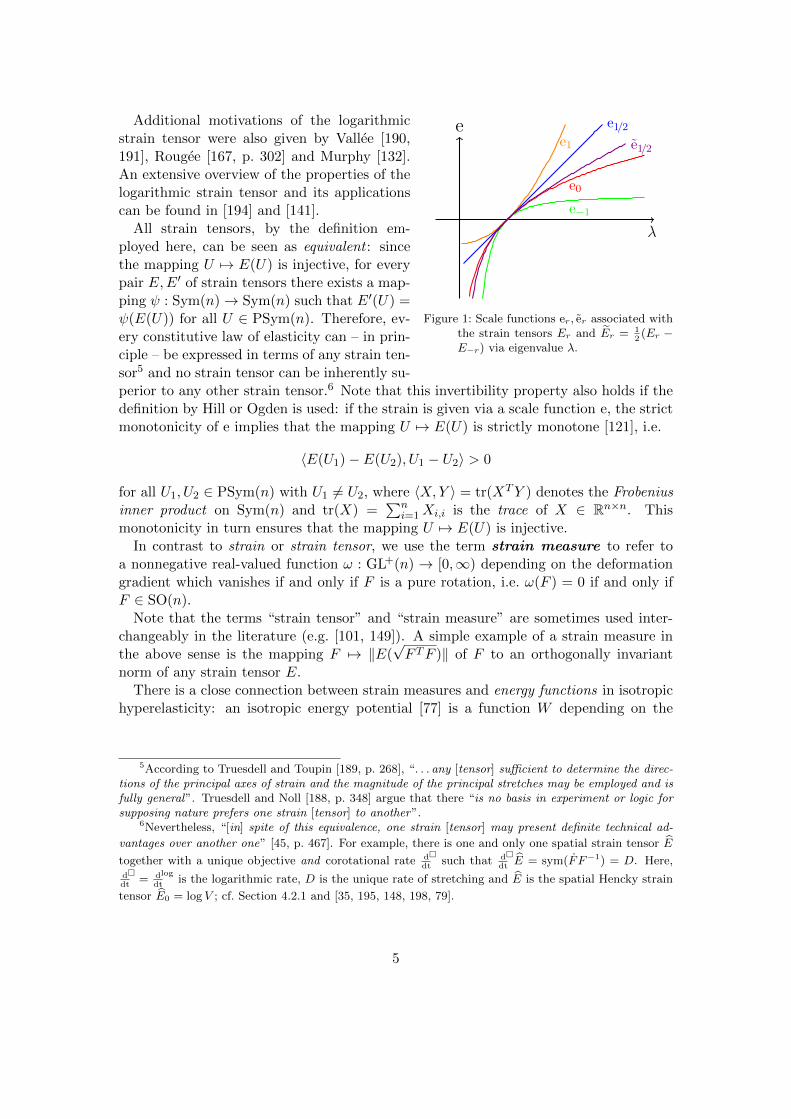
λ

ee1

e1/2

e−1

e0

e1/2

Figure 1: Scale functions er, er associated withthe strain tensors Er and Er = 1

2(Er −

E−r) via eigenvalue λ.

Additional motivations of the logarithmicstrain tensor were also given by Vallee [190,191], Rougee [167, p. 302] and Murphy [132].An extensive overview of the properties of thelogarithmic strain tensor and its applicationscan be found in [194] and [141].

All strain tensors, by the definition em-ployed here, can be seen as equivalent : sincethe mapping U 7→ E(U) is injective, for everypair E,E′ of strain tensors there exists a map-ping ψ : Sym(n)→ Sym(n) such that E′(U) =ψ(E(U)) for all U ∈ PSym(n). Therefore, ev-ery constitutive law of elasticity can – in prin-ciple – be expressed in terms of any strain ten-sor5 and no strain tensor can be inherently su-perior to any other strain tensor.6 Note that this invertibility property also holds if thedefinition by Hill or Ogden is used: if the strain is given via a scale function e, the strictmonotonicity of e implies that the mapping U 7→ E(U) is strictly monotone [121], i.e.

〈E(U1)− E(U2), U1 − U2〉 > 0

for all U1, U2 ∈ PSym(n) with U1 6= U2, where 〈X,Y 〉 = tr(XTY ) denotes the Frobeniusinner product on Sym(n) and tr(X) =

∑ni=1Xi,i is the trace of X ∈ Rn×n. This

monotonicity in turn ensures that the mapping U 7→ E(U) is injective.In contrast to strain or strain tensor, we use the term strain measure to refer to

a nonnegative real-valued function ω : GL+(n) → [0,∞) depending on the deformationgradient which vanishes if and only if F is a pure rotation, i.e. ω(F ) = 0 if and only ifF ∈ SO(n).

Note that the terms “strain tensor” and “strain measure” are sometimes used inter-changeably in the literature (e.g. [101, 149]). A simple example of a strain measure inthe above sense is the mapping F 7→ ‖E(

√F TF )‖ of F to an orthogonally invariant

norm of any strain tensor E.There is a close connection between strain measures and energy functions in isotropic

hyperelasticity: an isotropic energy potential [77] is a function W depending on the

5According to Truesdell and Toupin [189, p. 268], “. . . any [tensor] sufficient to determine the direc-tions of the principal axes of strain and the magnitude of the principal stretches may be employed and isfully general”. Truesdell and Noll [188, p. 348] argue that there “is no basis in experiment or logic forsupposing nature prefers one strain [tensor] to another”.

6Nevertheless, “[in] spite of this equivalence, one strain [tensor] may present definite technical ad-

vantages over another one” [45, p. 467]. For example, there is one and only one spatial strain tensor E

together with a unique objective and corotational rate ddt

such that d

dt

E = sym(FF−1) = D. Here,

ddt

= d

dt

logis the logarithmic rate, D is the unique rate of stretching and E is the spatial Hencky strain

tensor E0 = log V ; cf. Section 4.2.1 and [35, 195, 148, 198, 79].

5

deformation gradient F such that

W (F ) ≥ 0 , (normalization)

W (QF ) = W (F ) , (frame-indifference)

W (FQ) = W (F ) (material symmetry: isotropy)

for all F ∈ GL+(n), Q ∈ SO(n) and

W (F ) = 0 if and only if F ∈ SO(n) . (stress-free reference configuration)

While every such energy function can be taken as a strain measure, many additional con-ditions for “proper” energy functions are discussed in the literature, such as constitutiveinequalities [187, 11, 42, 118], generalized convexity conditions [10, 13] or monotonicityconditions to ensure that “stress increases with strain” [141, Section 2.2]. Apart fromthat, the main difference between strain measures and energy functions is that the formerare purely mathematical expressions used to quantitatively assess the extent of strainin a deformation, whereas the latter postulate some physical behaviour of materials ina condensed form: an elastic energy potential, interpreted as the elastic energy per unitvolume in the undeformed configuration, induces a specific stress response function7,and therefore completely determines the physical behaviour of the modelled hyperelasticmaterial. The connection between “natural” strain measures and energy functions willbe further discussed later on.

In particular, we will be interested in energy potentials which can be expressed interms of certain strain measures. Note carefully that, in contrast to strain tensors,strain measures cannot simply be used interchangeably: for two different strain mea-sures (as defined above) ω1, ω2, there is generally no function f : R+ → R+ such thatω2(F ) = f(ω1(F )) for all F ∈ GL+(n). Compared to “full” strain tensors, this can beinterpreted as an unavoidable loss of information for strain measures (which are onlyscalar quantities).

Sometimes a strain measure is employed only for a particular kind of deformation.For example, on the group of simple shear deformations (in a fixed plane) consisting ofall Fγ ∈ GL+(3) of the form

Fγ =(

1 γ 00 1 00 0 1

), γ ∈ R ,

we could consider the mappings

Fγ 7→1

2γ2 , Fγ 7→

1√3|γ| or Fγ 7→

2√3

ln

(γ

2+

√1 +

γ2

4

);

the latter two are the von Mises equivalent strain [26] and the Hencky equivalent strain[154, 176] in simple shear. The expression |γ| is also referred to as the amount of shear

7The specific elasticity tensor further depends on the particular choice of a strain and a stress tensorin which to express the constitutive law.

6

[18, p. 25; 188, p. 174]. We will come back to these partial strain measures in Section3.2.

In the following we consider the question of what strain measures are appropriate forthe theory of nonlinear isotropic elasticity. Since, by our definition, a strain measureattains zero if and only if F ∈ SO(n), a simple geometric approach is to consider adistance function on the group GL+(n) of admissible deformation gradients, i.e. a sym-metric function dist : GL+(n)×GL+(n)→ [0,∞) which satisfies the triangle inequalityand vanishes if and only if its arguments are identical.8 Such a distance function inducesa “natural” strain measure on GL+(n) by means of the distance to the special orthogonalgroup SO(n):

ω(F ) := dist(F,SO(n)) := infQ∈SO(n)

dist(F,Q) . (5)

In this way, the search for an appropriate strain measure reduces to the task of findinga natural, intrinsic distance function on GL+(n).

1.2. The search for appropriate strain measures

The remainder of this article is dedicated to this task: after some simple (Euclidean)examples in Section 2, we consider the geodesic distance on GL+(n) in Section 3. Ourmain result is stated in Theorem 3.3: if the distance on GL+(n) is induced by a left-GL(n)-invariant, right-O(n)-invariant Riemannian metric on GL(n), then the distanceof F ∈ GL+(n) to SO(n) is given by

dist2geod(F,SO(n)) = dist2

geod(F,R) = µ ‖ devn logU‖2 +κ

2[tr(logU)]2 ,

where F = RU with U =√F TF ∈ PSym(n) and R ∈ SO(n) is the polar decomposition

of F . Section 3 also contains some additional remarks and corollaries which furtherexpand upon this Riemannian strain measure.

In Section 4, we discuss a number of different approaches towards motivating the useof logarithmic strain measures and strain tensors, whereas applications of our resultsand further research topics are indicated in Section 5.

Our main result (Theorem 3.3) has previously been announced in a Comptes RendusMecanique article [138] as well as in Proceedings in Applied Mathematics and Mechanics[137].

The idea for this paper has been conceived in late 2006. However, a number of technicaldifficulties had to be overcome (cf. [29, 146, 110, 119, 135]) in order to prove our results.The completion of this article might have taken more time than was originally foreseen,but we adhere to the old German saying: Gut Ding will Weile haben.

8A distance function is more commonly known as a metric of a metric space. The term “distance” isused here and throughout the article in order to avoid confusion with the Riemannian metric introducedlater on.

7

2. Euclidean strain measures

2.1. The Euclidean strain measure in linear isotropic elasticity

A similar approach to the definition of strain measures via distance functions on GL+(n),as stated in equation (5), can be employed in linearized elasticity theory: let ϕ(x) =x+u(x) with the displacement u. Then the infinitesimal strain measure may be obtainedby taking the distance of the displacement gradient ∇u ∈ Rn×n to the set of linearizedrotations so(n) = A ∈ Rn×n : AT = −A, which is the vector space9 of skew symmetricmatrices. An obvious choice for a distance measure on the linear space Rn×n ∼= Rn2

isthe Euclidean distance induced by the canonical Frobenius norm

‖X‖ =√

tr(XTX) =

√n∑

i,j=1

X2ij .

We use the more general weighted norm defined by

‖X‖2µ,µc,κ = µ ‖devn symX‖2 + µc ‖ skewX‖2 +κ

2[tr(X)]2 , µ, µc, κ > 0 , (6)

which separately weights the deviatoric (or trace free) symmetric part devn symX =symX − 1

n tr(symX) · 1, the spherical part 1n tr(X) · 1, and the skew symmetric part

skewX = 12(X −XT ) of X; note that ‖X‖µ,µc,κ = ‖X‖ for µ = µc = 1, κ = 2

n , and that

‖ . ‖µ,µc,κ is induced by the inner product10

〈X,Y 〉µ,µc,κ = µ 〈devn symX,devn symY 〉+ µc 〈skewX, skew Y 〉+ κ2 tr(X) tr(Y ) (7)

on Rn×n, where 〈X,Y 〉 = tr(XTY ) denotes the canonical inner product. In fact, everyisotropic inner product on Rn×n, i.e. every inner product 〈·, ·〉iso with

〈QX,QY 〉iso = 〈XQ,Y Q〉iso = 〈X,Y 〉iso

for all X,Y ∈ Rn×n and all Q ∈ O(n), is of the form (7), cf. [47]. The suggestive choice ofvariables µ and κ, which represent the shear modulus and the bulk modulus, respectively,will prove to be justified later on. The remaining parameter µc will be called the spinmodulus.

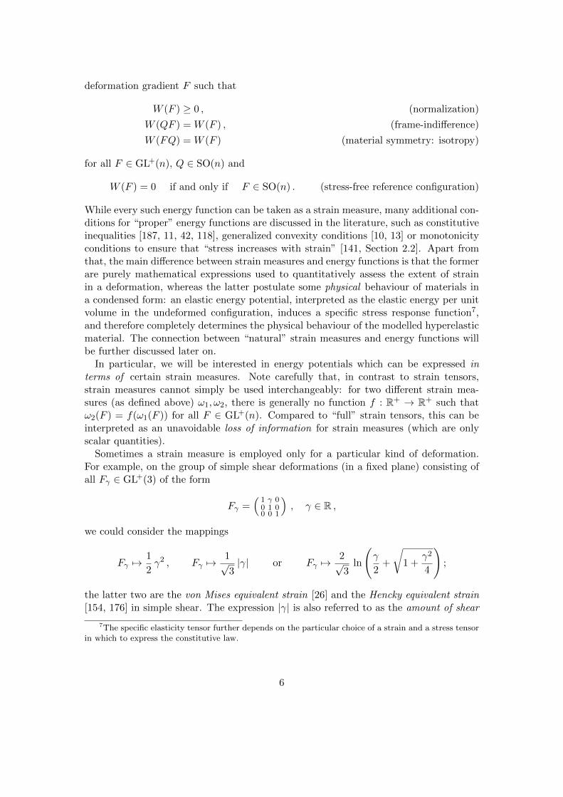
Of course, the element of best approximation in so(n) to ∇u with respect to theweighted Euclidean distance distEuclid,µ,µc,κ(X,Y ) = ‖X − Y ‖µ,µc,κ is given by the as-sociated orthogonal projection of ∇u to so(n), cf. Figure 2. Since so(n) and the spaceSym(n) of symmetric matrices are orthogonal with respect to 〈·, ·〉µ,µc,κ, this projection is

9Note that so(n) also corresponds to the Lie algebra of the special orthogonal group SO(n).10The family (7) of inner products on Rn×n is based on the Cartan-orthogonal decomposition

gl(n) =(sl(n) ∩ Sym(n)

)⊕ so(n)⊕ R · 1

of the Lie algebra gl(n) = Rn×n. Here, sl(n) = X ∈ gl(n) | trX = 0 denotes the Lie algebra corre-sponding to the special linear group SL(n) = A ∈ GL(n) | detA = 1.

8

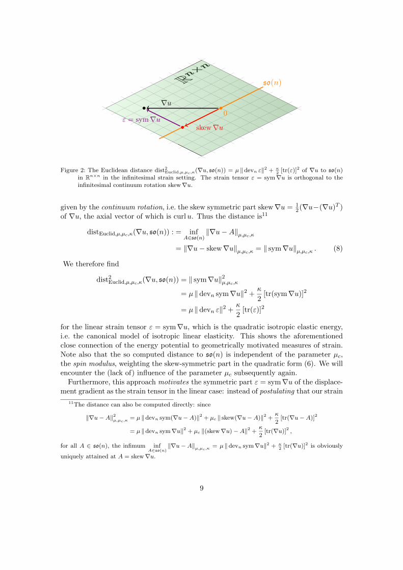
so(n)Rn×n

0ε = sym∇u

skew∇u

∇u

Figure 2: The Euclidean distance dist2Euclid,µ,µc,κ(∇u, so(n)) = µ ‖ devn ε‖2 + κ

2[tr(ε)]2 of ∇u to so(n)

in Rn×n in the infinitesimal strain setting. The strain tensor ε = sym∇u is orthogonal to theinfinitesimal continuum rotation skew∇u.

given by the continuum rotation, i.e. the skew symmetric part skew∇u = 12(∇u−(∇u)T )

of ∇u, the axial vector of which is curlu. Thus the distance is11

distEuclid,µ,µc,κ(∇u, so(n)) : = infA∈so(n)

‖∇u−A‖µ,µc,κ= ‖∇u− skew∇u‖µ,µc,κ = ‖ sym∇u‖µ,µc,κ . (8)

We therefore find

dist2Euclid,µ,µc,κ(∇u, so(n)) = ‖ sym∇u‖2µ,µc,κ

= µ ‖ devn sym∇u‖2 +κ

2[tr(sym∇u)]2

= µ ‖devn ε‖2 +κ

2[tr(ε)]2

for the linear strain tensor ε = sym∇u, which is the quadratic isotropic elastic energy,i.e. the canonical model of isotropic linear elasticity. This shows the aforementionedclose connection of the energy potential to geometrically motivated measures of strain.Note also that the so computed distance to so(n) is independent of the parameter µc,the spin modulus, weighting the skew-symmetric part in the quadratic form (6). We willencounter the (lack of) influence of the parameter µc subsequently again.

Furthermore, this approach motivates the symmetric part ε = sym∇u of the displace-ment gradient as the strain tensor in the linear case: instead of postulating that our strain

11The distance can also be computed directly: since

‖∇u−A‖2µ,µc,κ= µ ‖devn sym(∇u−A)‖2 + µc ‖ skew(∇u−A)‖2 +

κ

2[tr(∇u−A)]2

= µ ‖devn sym∇u‖2 + µc ‖(skew∇u)−A‖2 +κ

2[tr(∇u)]2 ,

for all A ∈ so(n), the infimum infA∈so(n)

‖∇u−A‖µ,µc,κ= µ ‖devn sym∇u‖2 + κ

2[tr(∇u)]2 is obviously

uniquely attained at A = skew∇u.

9

measure should depend only on ε, the above computations deductively characterize ε asthe infinitesimal strain tensor from simple geometric assumptions alone.

2.2. The Euclidean strain measure in nonlinear isotropic elasticity

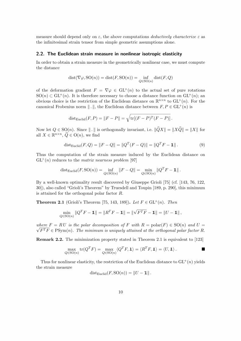
In order to obtain a strain measure in the geometrically nonlinear case, we must computethe distance

dist(∇ϕ,SO(n)) = dist(F,SO(n)) = infQ∈SO(n)

dist(F,Q)

of the deformation gradient F = ∇ϕ ∈ GL+(n) to the actual set of pure rotationsSO(n) ⊂ GL+(n). It is therefore necessary to choose a distance function on GL+(n); anobvious choice is the restriction of the Euclidean distance on Rn×n to GL+(n). For thecanonical Frobenius norm ‖ . ‖, the Euclidean distance between F, P ∈ GL+(n) is

distEuclid(F, P ) = ‖F − P‖ =√

tr[(F − P )T (F − P )] .

Now let Q ∈ SO(n). Since ‖ . ‖ is orthogonally invariant, i.e. ‖QX‖ = ‖XQ‖ = ‖X‖ forall X ∈ Rn×n, Q ∈ O(n), we find

distEuclid(F,Q) = ‖F −Q‖ = ‖QT (F −Q)‖ = ‖QTF − 1‖ . (9)

Thus the computation of the strain measure induced by the Euclidean distance onGL+(n) reduces to the matrix nearness problem [97]

distEuclid(F,SO(n)) = infQ∈SO(n)

‖F −Q‖ = minQ∈SO(n)

‖QTF − 1‖ .

By a well-known optimality result discovered by Giuseppe Grioli [75] (cf. [143, 76, 122,30]), also called “Grioli’s Theorem” by Truesdell and Toupin [189, p. 290], this minimumis attained for the orthogonal polar factor R.

Theorem 2.1 (Grioli’s Theorem [75, 143, 189]). Let F ∈ GL+(n). Then

minQ∈SO(n)

‖QTF − 1‖ = ‖RTF − 1‖ = ‖√F TF − 1‖ = ‖U − 1‖ ,

where F = RU is the polar decomposition of F with R = polar(F ) ∈ SO(n) and U =√F TF ∈ PSym(n). The minimum is uniquely attained at the orthogonal polar factor R.

Remark 2.2. The minimization property stated in Theorem 2.1 is equivalent to [123]

maxQ∈SO(n)

tr(QTF ) = maxQ∈SO(n)

〈QTF,1〉 = 〈RTF,1〉 = 〈U,1〉 .

Thus for nonlinear elasticity, the restriction of the Euclidean distance to GL+(n) yieldsthe strain measure

distEuclid(F,SO(n)) = ‖U − 1‖ .

10

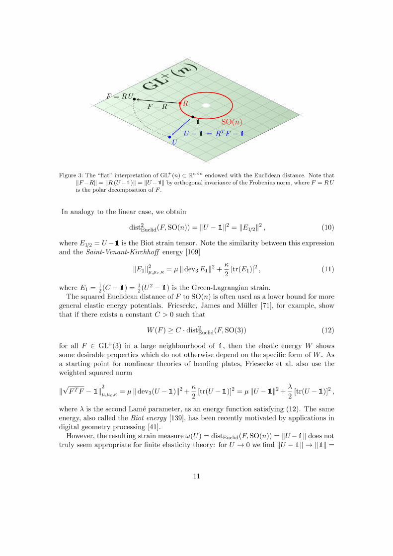
GL+(n

)

SO(n)

F −R

U − 1 = RTF − 1

R

1

F = RU

U

Figure 3: The “flat” interpretation of GL+(n) ⊂ Rn×n endowed with the Euclidean distance. Note that‖F−R‖ = ‖R (U−1)‖ = ‖U−1‖ by orthogonal invariance of the Frobenius norm, where F = RUis the polar decomposition of F .

In analogy to the linear case, we obtain

dist2Euclid(F,SO(n)) = ‖U − 1‖2 = ‖E1/2‖2 , (10)

where E1/2 = U−1 is the Biot strain tensor. Note the similarity between this expressionand the Saint-Venant-Kirchhoff energy [109]

‖E1‖2µ,µc,κ = µ ‖ dev3E1‖2 +κ

2[tr(E1)]2 , (11)

where E1 = 12(C − 1) = 1

2(U2 − 1) is the Green-Lagrangian strain.The squared Euclidean distance of F to SO(n) is often used as a lower bound for more

general elastic energy potentials. Friesecke, James and Muller [71], for example, showthat if there exists a constant C > 0 such that

W (F ) ≥ C · dist2Euclid(F,SO(3)) (12)

for all F ∈ GL+(3) in a large neighbourhood of 1, then the elastic energy W showssome desirable properties which do not otherwise depend on the specific form of W . Asa starting point for nonlinear theories of bending plates, Friesecke et al. also use theweighted squared norm

‖√F TF − 1‖2µ,µc,κ = µ ‖ dev3(U −1)‖2 +

κ

2[tr(U −1)]2 = µ ‖U −1‖2 +

λ

2[tr(U −1)]2 ,

where λ is the second Lame parameter, as an energy function satisfying (12). The sameenergy, also called the Biot energy [139], has been recently motivated by applications indigital geometry processing [41].

However, the resulting strain measure ω(U) = distEuclid(F,SO(n)) = ‖U−1‖ does nottruly seem appropriate for finite elasticity theory: for U → 0 we find ‖U −1‖ → ‖1‖ =

11

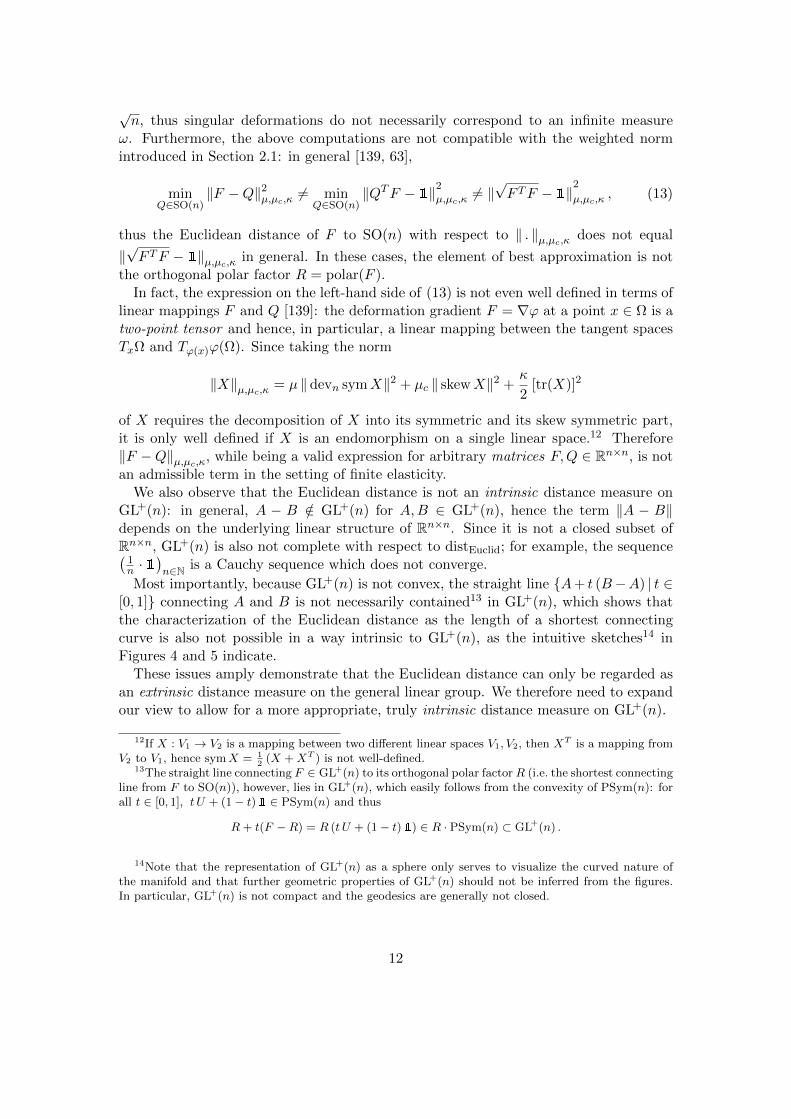
√n, thus singular deformations do not necessarily correspond to an infinite measure

ω. Furthermore, the above computations are not compatible with the weighted normintroduced in Section 2.1: in general [139, 63],

minQ∈SO(n)

‖F −Q‖2µ,µc,κ 6= minQ∈SO(n)

‖QTF − 1‖2µ,µc,κ 6= ‖√F TF − 1‖2µ,µc,κ , (13)

thus the Euclidean distance of F to SO(n) with respect to ‖ . ‖µ,µc,κ does not equal

‖√F TF − 1‖µ,µc,κ in general. In these cases, the element of best approximation is not

the orthogonal polar factor R = polar(F ).In fact, the expression on the left-hand side of (13) is not even well defined in terms of

linear mappings F and Q [139]: the deformation gradient F = ∇ϕ at a point x ∈ Ω is atwo-point tensor and hence, in particular, a linear mapping between the tangent spacesTxΩ and Tϕ(x)ϕ(Ω). Since taking the norm

‖X‖µ,µc,κ = µ ‖ devn symX‖2 + µc ‖ skewX‖2 +κ

2[tr(X)]2

of X requires the decomposition of X into its symmetric and its skew symmetric part,it is only well defined if X is an endomorphism on a single linear space.12 Therefore‖F −Q‖µ,µc,κ, while being a valid expression for arbitrary matrices F,Q ∈ Rn×n, is notan admissible term in the setting of finite elasticity.

We also observe that the Euclidean distance is not an intrinsic distance measure onGL+(n): in general, A − B /∈ GL+(n) for A,B ∈ GL+(n), hence the term ‖A − B‖depends on the underlying linear structure of Rn×n. Since it is not a closed subset ofRn×n, GL+(n) is also not complete with respect to distEuclid; for example, the sequence(

1n · 1

)n∈N is a Cauchy sequence which does not converge.

Most importantly, because GL+(n) is not convex, the straight line A+ t (B−A) | t ∈[0, 1] connecting A and B is not necessarily contained13 in GL+(n), which shows thatthe characterization of the Euclidean distance as the length of a shortest connectingcurve is also not possible in a way intrinsic to GL+(n), as the intuitive sketches14 inFigures 4 and 5 indicate.

These issues amply demonstrate that the Euclidean distance can only be regarded asan extrinsic distance measure on the general linear group. We therefore need to expandour view to allow for a more appropriate, truly intrinsic distance measure on GL+(n).

12If X : V1 → V2 is a mapping between two different linear spaces V1, V2, then XT is a mapping fromV2 to V1, hence symX = 1

2(X +XT ) is not well-defined.

13The straight line connecting F ∈ GL+(n) to its orthogonal polar factorR (i.e. the shortest connectingline from F to SO(n)), however, lies in GL+(n), which easily follows from the convexity of PSym(n): forall t ∈ [0, 1], t U + (1− t)1 ∈ PSym(n) and thus

R+ t(F −R) = R (t U + (1− t)1) ∈ R · PSym(n) ⊂ GL+(n) .

14Note that the representation of GL+(n) as a sphere only serves to visualize the curved nature ofthe manifold and that further geometric properties of GL+(n) should not be inferred from the figures.In particular, GL+(n) is not compact and the geodesics are generally not closed.

12

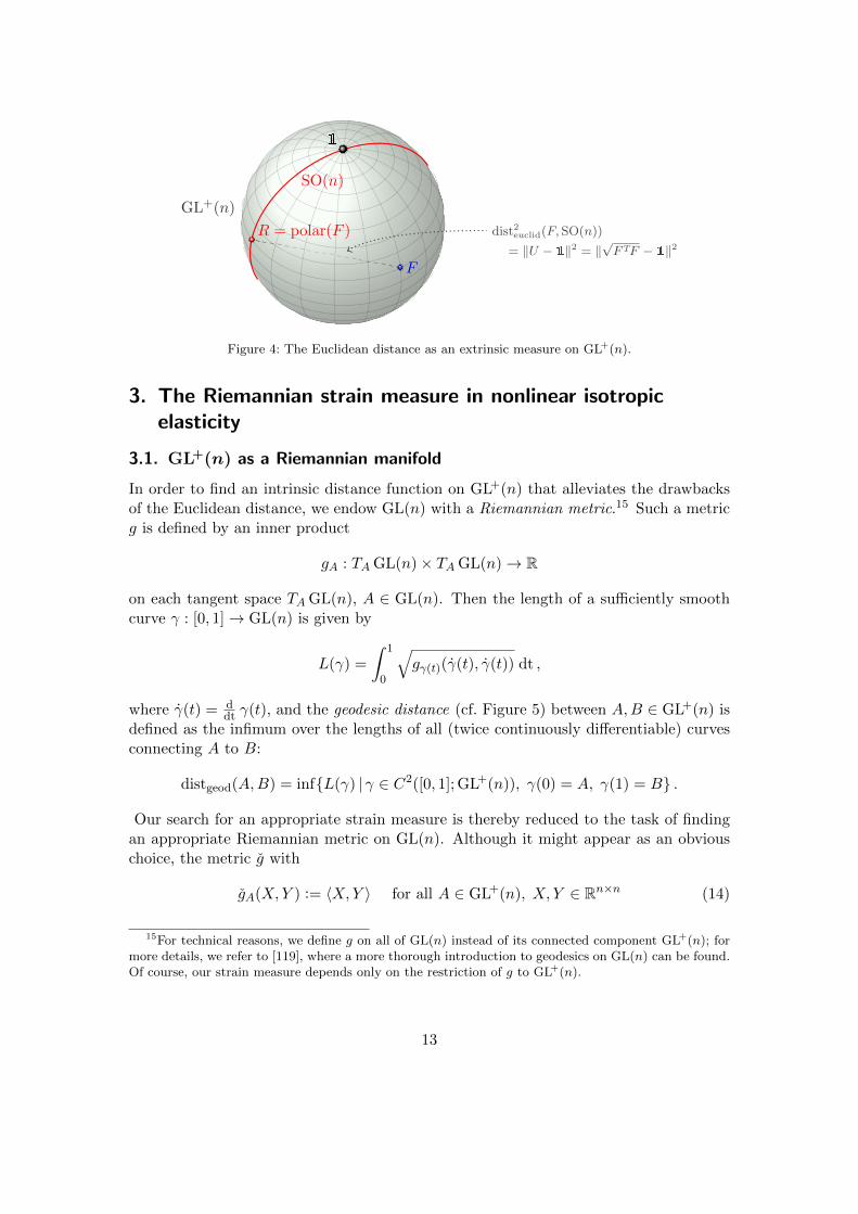
SO(n)

1

R = polar(F )

GL+(n)

F

dist2euclid(F,SO(n))

= ‖U − 1‖2 = ‖√FTF − 1‖2

Figure 4: The Euclidean distance as an extrinsic measure on GL+(n).

3. The Riemannian strain measure in nonlinear isotropicelasticity

3.1. GL+(n) as a Riemannian manifold

In order to find an intrinsic distance function on GL+(n) that alleviates the drawbacksof the Euclidean distance, we endow GL(n) with a Riemannian metric.15 Such a metricg is defined by an inner product

gA : TA GL(n)× TA GL(n)→ R

on each tangent space TA GL(n), A ∈ GL(n). Then the length of a sufficiently smoothcurve γ : [0, 1]→ GL(n) is given by

L(γ) =

∫ 1

0

√gγ(t)(γ(t), γ(t)) dt ,

where γ(t) = ddt γ(t), and the geodesic distance (cf. Figure 5) between A,B ∈ GL+(n) is

defined as the infimum over the lengths of all (twice continuously differentiable) curvesconnecting A to B:

distgeod(A,B) = infL(γ) | γ ∈ C2([0, 1]; GL+(n)), γ(0) = A, γ(1) = B .

Our search for an appropriate strain measure is thereby reduced to the task of findingan appropriate Riemannian metric on GL(n). Although it might appear as an obviouschoice, the metric g with

gA(X,Y ) := 〈X,Y 〉 for all A ∈ GL+(n), X, Y ∈ Rn×n (14)

15For technical reasons, we define g on all of GL(n) instead of its connected component GL+(n); formore details, we refer to [119], where a more thorough introduction to geodesics on GL(n) can be found.Of course, our strain measure depends only on the restriction of g to GL+(n).

13

AGL+(n) Bdist2euclid(A,B) = ‖A−B‖2

dist2geod(A,B)

Figure 5: The geodesic (intrinsic) distance compared to the Euclidean (extrinsic) distance.

provides no improvement over the already discussed Euclidean distance on GL+(n): sincethe length of a curve γ with respect to g is the classical (Euclidean) length

L(γ) =

∫ 1

0

√gγ(t)(γ(t), γ(t)) dt =

∫ 1

0‖γ(t)‖dt ,

the shortest connecting curves with respect to g are straight lines of the form t 7→A + t(B − A) with A,B ∈ GL+(n). Locally, the geodesic distance induced by g istherefore equal to the Euclidean distance. However, as discussed in the previous section,not all straight lines connecting arbitrary A,B ∈ GL+(n) are contained within GL+(n),thus length minimizing curves with respect to g do not necessarily exist (cf. Figure 6).Many of the shortcomings of the Euclidean distance therefore apply to the geodesicdistance induced by g as well.

GL+(n

)

γ(t) = A+ t(B −A)

γ(t0) /∈ GL+(n)

γ

AB

C

Figure 6: The shortest connecting (geodesic) curves in GL+(n) with respect to the Euclidean metricare straight lines, thus not every pair A,B ∈ GL+(n) can be connected by curves of minimallength. The length of the straight line γ : t 7→ A + t(C − A) connecting A to C is given by∫ 1

0

√gγ(t)(γ(t), γ(t)) dt = ‖C − A‖, whereas the curve γ connecting A to B is not contained in

GL+(n); its length is therefore not well defined.

In order to find a more viable Riemannian metric g on GL(n), we consider the me-chanical interpretation of the induced geodesic distance distgeod: while our focus lies onthe strain measure induced by g, that is the geodesic distance of the deformation gradi-ent F to the special orthogonal group SO(n), the distance distgeod(F1, F2) between twodeformation gradients F1, F2 can also be motivated directly as a measure of differencebetween two linear (or homogeneous) deformations F1, F2 of the same body Ω. Moregenerally, we can define a difference measure between two inhomogeneous deformations

14

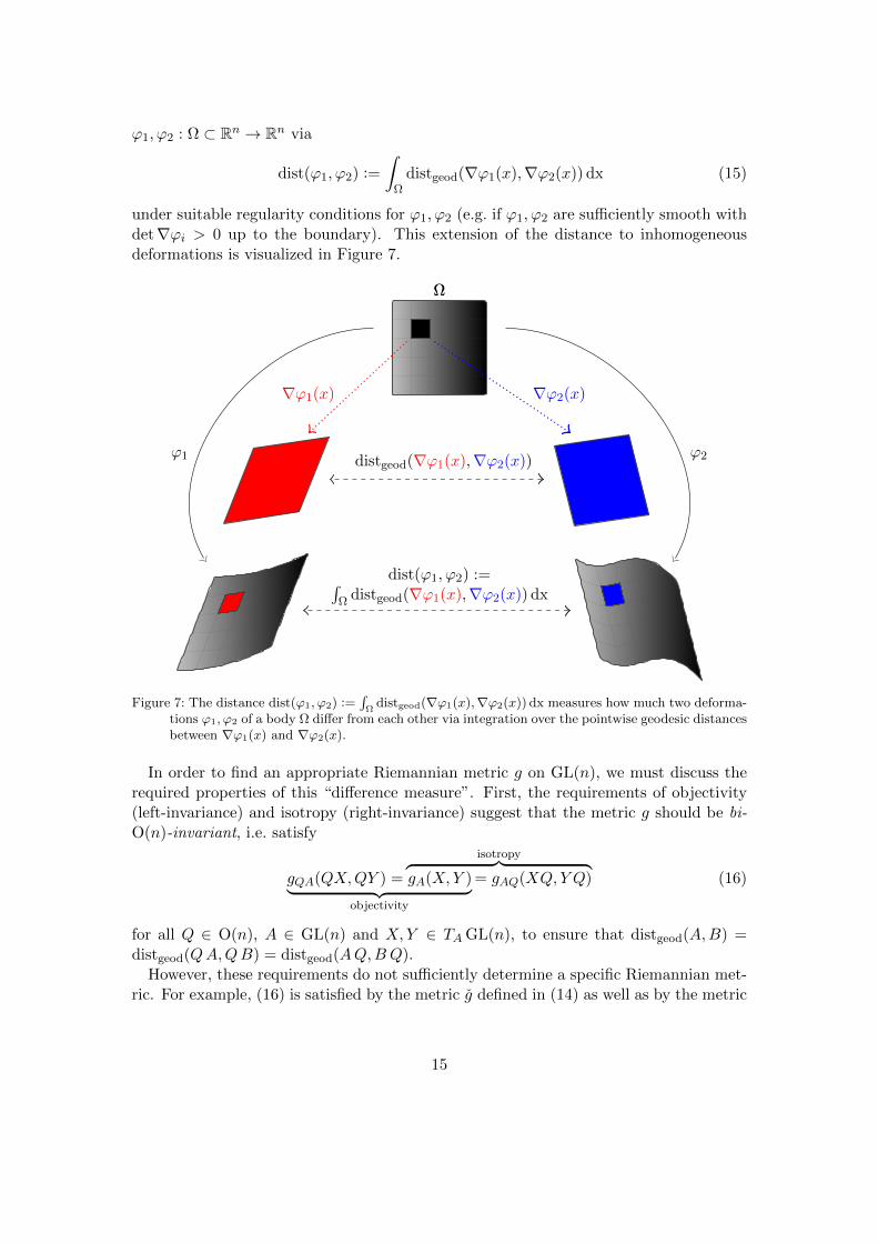
ϕ1, ϕ2 : Ω ⊂ Rn → Rn via

dist(ϕ1, ϕ2) :=

∫

Ωdistgeod(∇ϕ1(x),∇ϕ2(x)) dx (15)

under suitable regularity conditions for ϕ1, ϕ2 (e.g. if ϕ1, ϕ2 are sufficiently smooth withdet∇ϕi > 0 up to the boundary). This extension of the distance to inhomogeneousdeformations is visualized in Figure 7.

x

ϕ1 ϕ2

∇ϕ1(x) ∇ϕ2(x)

distgeod(∇ϕ1(x),∇ϕ2(x))

dist(ϕ1, ϕ2) :=∫Ω distgeod(∇ϕ1(x),∇ϕ2(x)) dx

ΩΩ

Figure 7: The distance dist(ϕ1, ϕ2) :=∫

Ωdistgeod(∇ϕ1(x),∇ϕ2(x)) dx measures how much two deforma-

tions ϕ1, ϕ2 of a body Ω differ from each other via integration over the pointwise geodesic distancesbetween ∇ϕ1(x) and ∇ϕ2(x).

In order to find an appropriate Riemannian metric g on GL(n), we must discuss therequired properties of this “difference measure”. First, the requirements of objectivity(left-invariance) and isotropy (right-invariance) suggest that the metric g should be bi-O(n)-invariant, i.e. satisfy

gQA(QX,QY ) = gA(X,Y )︸︷︷︸objectivity

isotropy︷︸︸︷= gAQ(XQ,Y Q) (16)

for all Q ∈ O(n), A ∈ GL(n) and X,Y ∈ TA GL(n), to ensure that distgeod(A,B) =distgeod(QA,QB) = distgeod(AQ,B Q).

However, these requirements do not sufficiently determine a specific Riemannian met-ric. For example, (16) is satisfied by the metric g defined in (14) as well as by the metric

15

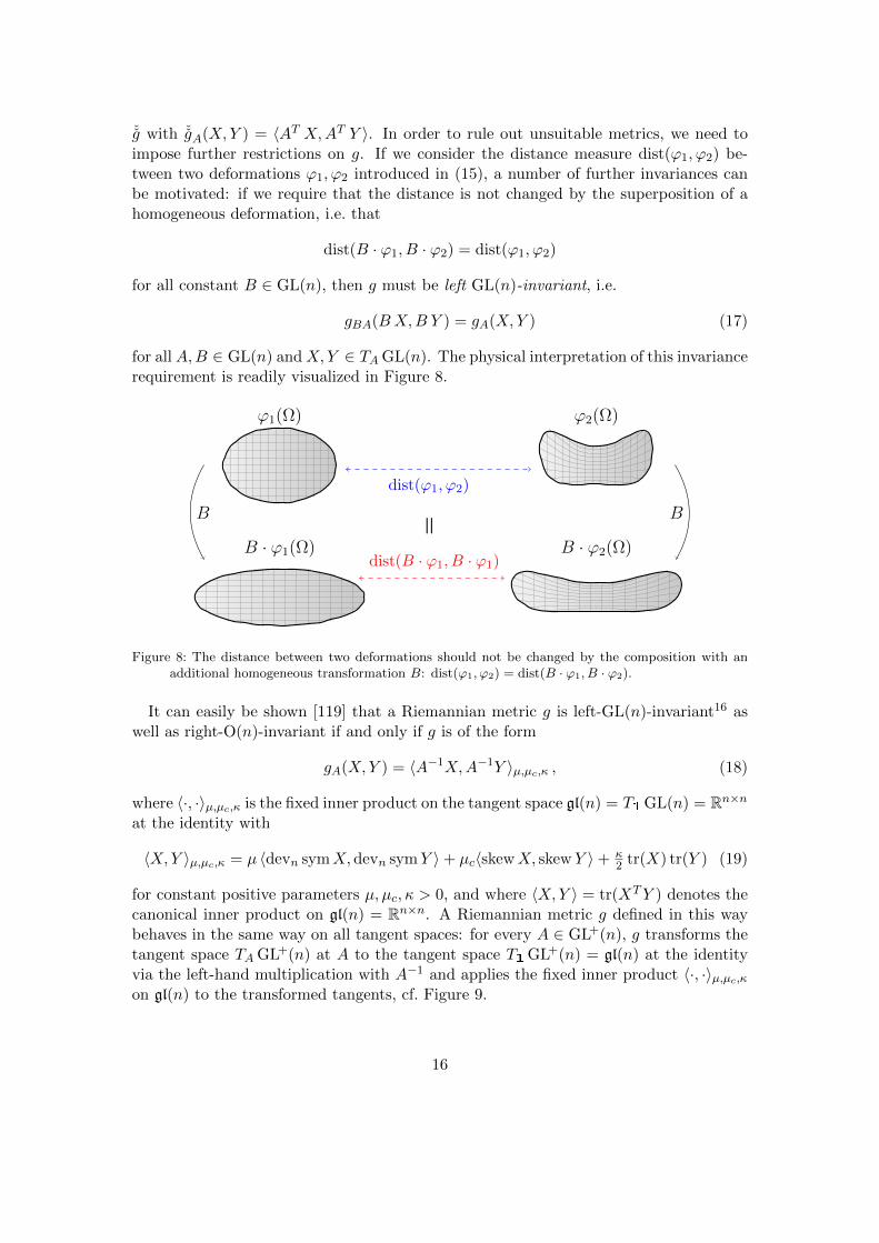
ˇg with ˇgA(X,Y ) = 〈AT X,AT Y 〉. In order to rule out unsuitable metrics, we need toimpose further restrictions on g. If we consider the distance measure dist(ϕ1, ϕ2) be-tween two deformations ϕ1, ϕ2 introduced in (15), a number of further invariances canbe motivated: if we require that the distance is not changed by the superposition of ahomogeneous deformation, i.e. that

dist(B · ϕ1, B · ϕ2) = dist(ϕ1, ϕ2)

for all constant B ∈ GL(n), then g must be left GL(n)-invariant, i.e.

gBA(BX,B Y ) = gA(X,Y ) (17)

for all A,B ∈ GL(n) andX,Y ∈ TA GL(n). The physical interpretation of this invariancerequirement is readily visualized in Figure 8.

B B

ϕ1(Ω) ϕ2(Ω)

B · ϕ1(Ω) B · ϕ2(Ω)

dist(ϕ1, ϕ2)

dist(B · ϕ1, B · ϕ1)

=

Figure 8: The distance between two deformations should not be changed by the composition with anadditional homogeneous transformation B: dist(ϕ1, ϕ2) = dist(B · ϕ1, B · ϕ2).

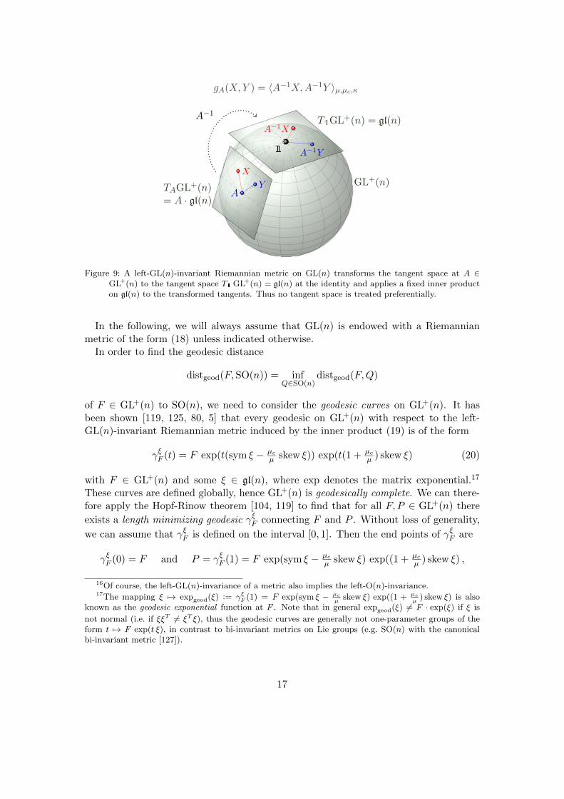
It can easily be shown [119] that a Riemannian metric g is left-GL(n)-invariant16 aswell as right-O(n)-invariant if and only if g is of the form

gA(X,Y ) = 〈A−1X,A−1Y 〉µ,µc,κ , (18)

where 〈·, ·〉µ,µc,κ is the fixed inner product on the tangent space gl(n) = T1 GL(n) = Rn×nat the identity with

〈X,Y 〉µ,µc,κ = µ 〈devn symX,devn symY 〉+ µc〈skewX, skew Y 〉+ κ2 tr(X) tr(Y ) (19)

for constant positive parameters µ, µc, κ > 0, and where 〈X,Y 〉 = tr(XTY ) denotes thecanonical inner product on gl(n) = Rn×n. A Riemannian metric g defined in this waybehaves in the same way on all tangent spaces: for every A ∈ GL+(n), g transforms thetangent space TA GL+(n) at A to the tangent space T1 GL+(n) = gl(n) at the identityvia the left-hand multiplication with A−1 and applies the fixed inner product 〈·, ·〉µ,µc,κon gl(n) to the transformed tangents, cf. Figure 9.

16

GL+(n)TAGL+(n)= A · gl(n)

T1GL+(n) = gl(n)

1

A

X

Y

A−1X

A−1Y

A−1

gA(X,Y ) = 〈A−1X,A−1Y 〉µ,µc,κ

Figure 9: A left-GL(n)-invariant Riemannian metric on GL(n) transforms the tangent space at A ∈GL+(n) to the tangent space T1 GL+(n) = gl(n) at the identity and applies a fixed inner producton gl(n) to the transformed tangents. Thus no tangent space is treated preferentially.

In the following, we will always assume that GL(n) is endowed with a Riemannianmetric of the form (18) unless indicated otherwise.

In order to find the geodesic distance

distgeod(F,SO(n)) = infQ∈SO(n)

distgeod(F,Q)

of F ∈ GL+(n) to SO(n), we need to consider the geodesic curves on GL+(n). It hasbeen shown [119, 125, 80, 5] that every geodesic on GL+(n) with respect to the left-GL(n)-invariant Riemannian metric induced by the inner product (19) is of the form

γξF (t) = F exp(t(sym ξ − µcµ skew ξ)) exp(t(1 + µc

µ ) skew ξ) (20)

with F ∈ GL+(n) and some ξ ∈ gl(n), where exp denotes the matrix exponential.17

These curves are defined globally, hence GL+(n) is geodesically complete. We can there-fore apply the Hopf-Rinow theorem [104, 119] to find that for all F, P ∈ GL+(n) there

exists a length minimizing geodesic γξF connecting F and P . Without loss of generality,

we can assume that γξF is defined on the interval [0, 1]. Then the end points of γξF are

γξF (0) = F and P = γξF (1) = F exp(sym ξ − µcµ skew ξ) exp((1 + µc

µ ) skew ξ) ,

16Of course, the left-GL(n)-invariance of a metric also implies the left-O(n)-invariance.17The mapping ξ 7→ expgeod(ξ) := γξF (1) = F exp(sym ξ − µc

µskew ξ) exp((1 + µc

µ) skew ξ) is also

known as the geodesic exponential function at F . Note that in general expgeod(ξ) 6= F · exp(ξ) if ξ is

not normal (i.e. if ξξT 6= ξT ξ), thus the geodesic curves are generally not one-parameter groups of theform t 7→ F exp(t ξ), in contrast to bi-invariant metrics on Lie groups (e.g. SO(n) with the canonicalbi-invariant metric [127]).

17

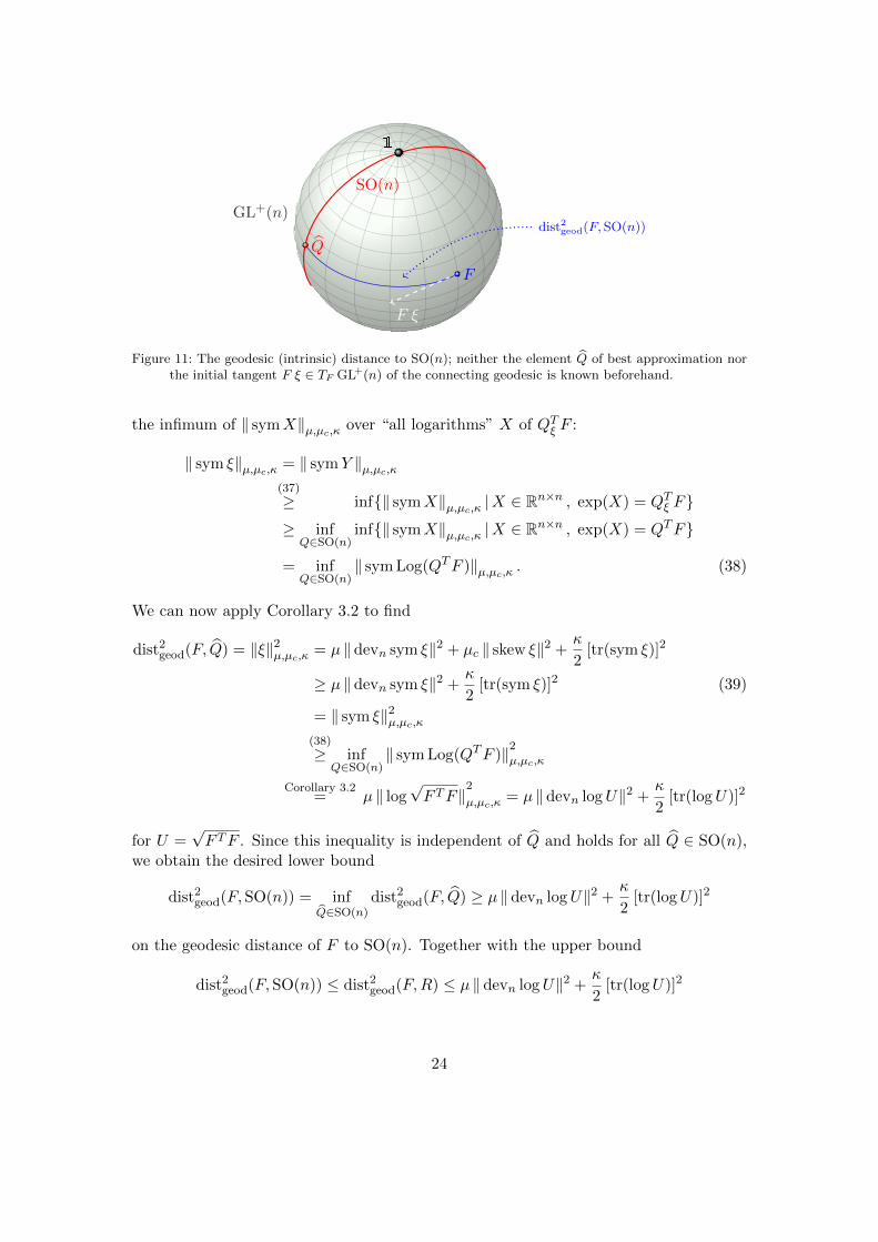
and the length of the geodesic γξF starting in F with initial tangent F ξ ∈ TF GL+(n)(cf. (20) and Figure 11) is given by [119]

L(γξF ) = ‖ξ‖µ,µc,κ .

The geodesic distance between F and P can therefore be characterized as

distgeod(F, P ) = min‖ξ‖µ,µc,κ | ξ ∈ gl(n) : γξF (1) = P ,

that is the minimum of ‖ξ‖µ,µc,κ over all ξ ∈ gl(n) which connect F and P , i.e. satisfy

exp(sym ξ − µcµ skew ξ) exp((1 + µc

µ ) skew ξ) = F−1P . (21)

Although some numerical computations have been employed [197] to approximate thegeodesic distance in the special case of the canonical left-GL(n)-invariant metric, i.e.for µ = µc = 1, κ = 2

n , there is no known closed form solution to the highly nonlinearsystem (21) in terms of ξ for given F, P ∈ GL+(n) and thus no known method of directlycomputing distgeod(F, P ) in the general case exists. However, this parametrization ofthe geodesic curves will allow us to obtain a lower bound on the distance of F to SO(n).

3.2. The geodesic distance to SO(n)

Having defined the geodesic distance on GL+(n), we can now consider the geodesic strainmeasure, which is the geodesic distance of the deformation gradient F to SO(n):


distgeod(F,Q) . (22)

Without explicit computation of this distance, the left-GL(n)-invariance and the right-O(n)-invariance of the metric g immediately allow us to show the inverse deformationsymmetry of the geodesic strain measure:


distgeod(F,Q) = infQ∈SO(n)

distgeod(F−1F, F−1Q)

= infQ∈SO(n)

distgeod(1, F−1Q) = infQ∈SO(n)

distgeod(QTQ,F−1Q)

= infQ∈SO(n)

distgeod(QT , F−1) = distgeod(F−1, SO(n)) . (23)

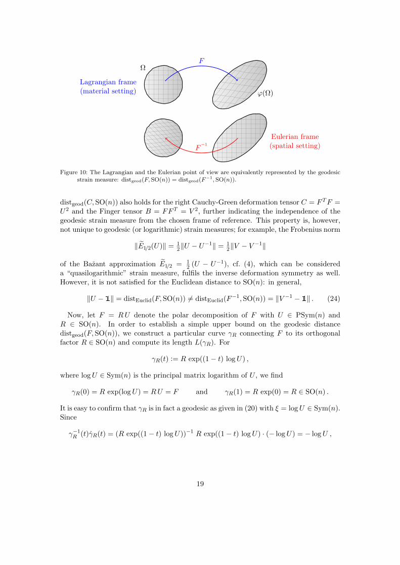
This symmetry property demonstrates that the Eulerian (spatial) and the Lagrangian(referential) points of view are equivalent with respect to the geodesic strain measure:in the Eulerian setting, the inverse F−1 of the deformation gradient appears more nat-urally18, whereas F is used in the Lagrangian frame (cf. Figure 10). Equality (23)shows that both points of view can equivalently be taken if the geodesic strain mea-sure is used. As we will see later on (Remark 3.5), the equality distgeod(B, SO(n)) =

18Note that Cauchy originally introduced the tensors C−1 and B−1 in his investigations of the nonlin-ear strain [39, 40, 70, 167], where C = FTF = U2 is the right Cauchy-Green deformation tensor [74, 70]and B = FFT = V 2 is the Finger tensor.

18

FΩ

ϕ(Ω)

F−1

Lagrangian frame(material setting)

Eulerian frame(spatial setting)

Figure 10: The Lagrangian and the Eulerian point of view are equivalently represented by the geodesicstrain measure: distgeod(F,SO(n)) = distgeod(F−1, SO(n)).

distgeod(C,SO(n)) also holds for the right Cauchy-Green deformation tensor C = F TF =U2 and the Finger tensor B = FF T = V 2, further indicating the independence of thegeodesic strain measure from the chosen frame of reference. This property is, however,not unique to geodesic (or logarithmic) strain measures; for example, the Frobenius norm

‖E1/2(U)‖ = 12‖U − U−1‖ = 1

2‖V − V −1‖

of the Bazant approximation E1/2 = 12 (U − U−1), cf. (4), which can be considered

a “quasilogarithmic” strain measure, fulfils the inverse deformation symmetry as well.However, it is not satisfied for the Euclidean distance to SO(n): in general,

‖U − 1‖ = distEuclid(F,SO(n)) 6= distEuclid(F−1, SO(n)) = ‖V −1 − 1‖ . (24)

Now, let F = RU denote the polar decomposition of F with U ∈ PSym(n) andR ∈ SO(n). In order to establish a simple upper bound on the geodesic distancedistgeod(F,SO(n)), we construct a particular curve γR connecting F to its orthogonalfactor R ∈ SO(n) and compute its length L(γR). For

γR(t) := R exp((1− t) logU) ,

where logU ∈ Sym(n) is the principal matrix logarithm of U , we find

γR(0) = R exp(logU) = RU = F and γR(1) = R exp(0) = R ∈ SO(n) .

It is easy to confirm that γR is in fact a geodesic as given in (20) with ξ = logU ∈ Sym(n).Since

γ−1R (t)γR(t) = (R exp((1− t) logU))−1 R exp((1− t) logU) · (− logU) = − logU ,

19

the length of γR is given by

L(γR) =

∫ 1

0

√gγR(t)(γR(t), γR(t)) dt (25)

=

∫ 1

0

√〈γR(t)−1γR(t), γR(t)−1γR(t)〉µ,µc,κ dt

=

∫ 1

0

√〈− logU,− logU〉µ,µc,κ dt =

∫ 1

0‖ logU‖µ,µc,κ dt = ‖ logU‖µ,µc,κ .

We can thereby establish the upper bound

dist2geod(F,SO(n)) = inf

Q∈SO(n)dist2

geod(F,Q) ≤ dist2geod(F,R) (26)

≤ L2(γR) = ‖ logU‖2µ,µc,κ = µ ‖ devn logU‖2 +κ

2[tr(logU)]2 (27)

for the geodesic distance of F to SO(n).Our task in the remainder of this section is to show that the right hand side of

inequality (27) is also a lower bound for the (squared) geodesic strain measure, i.e. that,altogether,

dist2geod(F,SO(n)) = µ ‖devn logU‖2 +

κ

2[tr(logU)]2 .

However, while the orthogonal polar factor R is the element of best approximationin the Euclidean case (for µ = µc = 1, κ = 2

n) due to Grioli’s Theorem, it is not clearwhether R is indeed the element in SO(n) with the shortest geodesic distance to F (andthus if equality holds in (26)). Furthermore, it is not even immediately obvious that thegeodesic distance between F and R is actually given by the right hand side of (27), sincea shorter connecting geodesic might exist (and hence inequality might hold in (27)).

Nonetheless, the following fundamental logarithmic minimization property19 of theorthogonal polar factor, combined with the computations in Section 3.1, allows us toshow that (27) is indeed also a lower bound for distgeod(F,SO(n)).

Proposition 3.1. Let F = R√F TF be the polar decomposition of F ∈ GL+(n) with

R ∈ SO(n) and let ‖ . ‖ denote the Frobenius norm on Rn×n. Then

infQ∈SO(n)

‖ sym Log(QTF )‖ = ‖ sym log(RTF )‖ = ‖ log√F TF‖ ,

where

infQ∈SO(n)

‖ sym Log(QTF )‖ := infQ∈SO(n)

inf‖ symX‖ | X ∈ Rn×n , exp(X) = QTF

is defined as the infimum of ‖ sym . ‖ over “all real matrix logarithms” of QTF .

19Of course, the application of such minimization properties to elasticity theory has a long tradition:Leonhard Euler, in the appendix “De curvis elasticis” to his 1744 book “Methodus inveniendi lineascurvas maximi minimive proprietate gaudentes sive solutio problematis isoperimetrici latissimo sensuaccepti” [56, 153], already proclaimed that “[. . . ] since the fabric of the universe is most perfect, and isthe work of a most wise creator, nothing whatsoever takes place in the universe in which some rule ofmaximum and minimum does not appear.”

20

Proposition 3.1, which can be seen as the natural logarithmic analogue of Grioli’sTheorem (cf. Section 2.2), was first shown for dimensions n = 2, 3 by Neff et al. [146]using the so-called sum-of-squared-logarithms inequality [29, 158, 46]. A generalizationto all unitarily invariant norms and complex logarithms for arbitrary dimension wasgiven by Lankeit, Neff and Nakatsukasa [110]. We also require the following corollaryinvolving the weighted Frobenius norm, which is not orthogonally invariant.20

Corollary 3.2. Let

‖X‖2µ,µc,κ = µ ‖ devn symX‖2 + µc ‖ skewX‖2 +κ

2[tr(X)]2 , µ, µc, κ > 0 ,

for all X ∈ Rn×n, where ‖ . ‖ is the Frobenius matrix norm. Then

infQ∈SO(n)

‖ sym Log(QTF )‖µ,µc,κ = ‖ log√F TF‖µ,µc,κ .

Proof. We first note that the equality det exp(X) = etr(X) holds for all X ∈ Rn×n. SincedetQ = 1 for all Q ∈ SO(n), this implies that for all X ∈ Rn×n with exp(X) = QTF ,

tr(symX) = tr(X) = ln(det(exp(X))) = ln(det(QTF )) = ln(detF ) .

Therefore21

‖ symX‖2µ,µc,κ= µ ‖ devn symX‖2 +

κ

2[tr(symX)]2

= µ ‖ symX‖2 +nκ− 2µ

2n[tr(symX)]2 = µ ‖ symX‖2 +

nκ− 2µ

2n(ln(detF ))2

and finally

infQ∈SO(n)

‖ sym Log(QTF )‖2µ,µc,κ (28)

= infQ∈SO(n)

inf‖ symX‖2µ,µc,κ |X ∈ Rn×n , exp(X) = QTF

= infQ∈SO(n)

infµ ‖ symX‖2 +nκ− 2µ

2n(ln(detF ))2 |X ∈ Rn×n , exp(X) = QTF

= µ infQ∈SO(n)

inf‖ symX‖2 |X ∈ Rn×n , exp(X) = QTF+nκ− 2µ

2n(ln(detF ))2

= µ‖ log√F TF‖2 +

nκ− 2µ

2n(ln(detF ))2

= µ‖ log√F TF‖2 +

nκ− 2µ

2n[tr(log

√F TF )]2

= µ ‖ devn log√F TF‖2 +

κ

2[tr(log

√F TF )]2 = ‖ log

√F TF‖2µ,µc,κ .

20While ‖QTXQ‖µ,µc,κ= ‖X‖µ,µc,κ

for all X ∈ Rn×n and Q ∈ O(n), the orthogonal invariancerequires the equalities ‖QX‖µ,µc,κ

= ‖XQ‖µ,µc,κ= ‖X‖µ,µc,κ

, which do not hold in general.21Observe that µ ‖ devn Y ‖2 + κ

2[tr(Y )]2 = µ ‖Y ‖2 + nκ−2µ

2n[tr(Y )]2 for all Y ∈ Rn×n.

21

Note that Corollary 3.2 also implies the weaker statement

infQ∈SO(n)

‖Log(QTF )‖µ,µc,κ = ‖ log√F TF‖µ,µc,κ

by using the simple estimate ‖X‖2µ,µc,κ ≥ ‖ symX‖2µ,µc,κ.

We are now ready to prove our main result.

Theorem 3.3. Let g be the left-GL(n)-invariant, right-O(n)-invariant Riemannian met-ric on GL(n) defined by

gA(X,Y ) = 〈A−1X,A−1Y 〉µ,µc,κ , µ, µc, κ > 0 ,

for A ∈ GL(n) and X,Y ∈ Rn×n, where

〈X,Y 〉µ,µc,κ = µ 〈devn symX,devn symY 〉+ µc〈skewX, skew Y 〉+ κ2 tr(X) tr(Y ) . (29)

Then for all F ∈ GL+(n), the geodesic distance of F to the special orthogonal groupSO(n) induced by g is given by

dist2geod(F,SO(n)) = µ ‖devn logU‖2 +

κ

2[tr(logU)]2 , (30)

where log is the principal matrix logarithm, tr(X) =∑n

i=1Xi,i denotes the trace anddevnX = X − 1

n tr(X) · 1 is the n-dimensional deviatoric part of X ∈ Rn×n. Theorthogonal factor R ∈ SO(n) of the polar decomposition F = RU is the unique elementof best approximation in SO(n), i.e.

distgeod(F,SO(n)) = distgeod(F,R) = distgeod(RTF,1) = distgeod(U,1) .

In particular, the geodesic distance does not depend on the spin modulus µc.

Remark 3.4 (Uniqueness of the metric). We remark once more that the Riemannianmetric considered in Theorem 3.3 is not chosen arbitrarily: every left-GL(n)-invariant,right-O(n)-invariant Riemannian metric on GL(n) is of the form given in (29) for somechoice of parameters µ, µc, κ > 0 [119].

Remark 3.5. Since the weighted Frobenius norm on the right hand side of equation(30) only depends on the eigenvalues of U =

√F TF , the result can also be expressed in

terms of the left Biot-stretch tensor V =√FF T , which has the same eigenvalues as U :

dist2geod(F,SO(n)) = µ ‖devn log V ‖2 +

κ

2[tr(log V )]2 . (31)

Applying the above formula to the case F = P with P ∈ PSym(n), we find√P TP =√

PP T = P and therefore

dist2(P,SO(n)) = dist2(P, 1) = µ ‖devn logP‖2 +κ

2[tr(logP )]2 , (32)

22

since 1 is the orthogonal polar factor of P . For the tensors U and V , the right Cauchy-Green deformation tensor C = F TF = U2 and the Finger tensor B = FF T = V 2, wethereby obtain the equalities

distgeod(B, SO(n)) = distgeod(B,1) = distgeod(B−1,1) (33)

= distgeod(C,1) = distgeod(C−1,1) = distgeod(C,SO(n))

and distgeod(V,SO(n)) = distgeod(V,1) = distgeod(V −1,1) (34)

= distgeod(U,1) = distgeod(U−1,1) = distgeod(U,SO(n)) .

Note carefully that, although (32) for P ∈ PSym(n) immediately follows from Theorem3.3, it is not trivial to compute the distance distgeod(P, 1) directly: while the curve givenby exp(t logP ) for t ∈ [0, 1] is in fact a geodesic [80] connecting 1 to P with lengthµ ‖devn logP‖2 + κ

2 [tr(logP )]2, it is not obvious whether or not a shorter connectinggeodesic might exist. Our result ensures that this is in fact not the case.

Proof of Theorem 3.3. Let F ∈ GL+(n) and Q ∈ SO(n). Then according to our previousconsiderations (cf. Section 3.1) there exists ξ ∈ gl(n) with


µ ) skew ξ) = F−1Q (35)

and‖ξ‖µ,µc,κ = distgeod(F, Q) . (36)

In order to find a lower estimate on ‖ξ‖µ,µc,κ (and thus on distgeod(F, Q)), we compute


µ ) skew ξ) = F−1Q

=⇒ exp((1 + µcµ ) skew ξ)−1 exp(sym ξ − µc

µ skew ξ)−1 = QTF

=⇒ exp(− sym ξ + µcµ skew ξ) = exp( (1 + µc

µ ) skew ξ︸︷︷︸

∈so(n)

) QTF .

Since exp(W ) ∈ SO(n) for all skew symmetric W ∈ so(n), we find

exp(− sym ξ + µcµ skew ξ

︸︷︷︸=:Y

) = QTξ F (37)

with Qξ = Q exp(−(1 + µcµ ) skew ξ ) ∈ SO(n); note that symY = − sym ξ. According

to (37), Y = − sym ξ + µcµ skew ξ is “a logarithm”22 of QTξ F . The weighted Frobenius

norm of the symmetric part of Y = − sym ξ+ µcµ skew ξ is therefore bounded below by

22Loosely speaking, we use the term “a logarithm of A ∈ GL+(n)” to denote any (real) solution X ofthe equation expX = A.

23

F ξ

SO(n)

1

GL+(n)

F

Q

dist2geod(F,SO(n))

Figure 11: The geodesic (intrinsic) distance to SO(n); neither the element Q of best approximation northe initial tangent F ξ ∈ TF GL+(n) of the connecting geodesic is known beforehand.

the infimum of ‖ symX‖µ,µc,κ over “all logarithms” X of QTξ F :

‖ sym ξ‖µ,µc,κ = ‖ symY ‖µ,µc,κ(37)

≥ inf‖ symX‖µ,µc,κ |X ∈ Rn×n , exp(X) = QTξ F≥ inf

Q∈SO(n)inf‖ symX‖µ,µc,κ |X ∈ Rn×n , exp(X) = QTF

= infQ∈SO(n)

‖ sym Log(QTF )‖µ,µc,κ . (38)

We can now apply Corollary 3.2 to find

dist2geod(F, Q) = ‖ξ‖2µ,µc,κ = µ ‖ devn sym ξ‖2 + µc ‖ skew ξ‖2 +

κ

2[tr(sym ξ)]2

≥ µ ‖devn sym ξ‖2 +κ

2[tr(sym ξ)]2 (39)

= ‖ sym ξ‖2µ,µc,κ(38)

≥ infQ∈SO(n)

‖ sym Log(QTF )‖2µ,µc,κCorollary 3.2

= µ ‖ log√F TF‖2µ,µc,κ = µ ‖ devn logU‖2 +

κ

2[tr(logU)]2

for U =√F TF . Since this inequality is independent of Q and holds for all Q ∈ SO(n),

we obtain the desired lower bound

dist2geod(F,SO(n)) = inf

Q∈SO(n)dist2

geod(F, Q) ≥ µ ‖ devn logU‖2 +κ

2[tr(logU)]2

on the geodesic distance of F to SO(n). Together with the upper bound

dist2geod(F,SO(n)) ≤ dist2

geod(F,R) ≤ µ ‖ devn logU‖2 +κ

2[tr(logU)]2

24

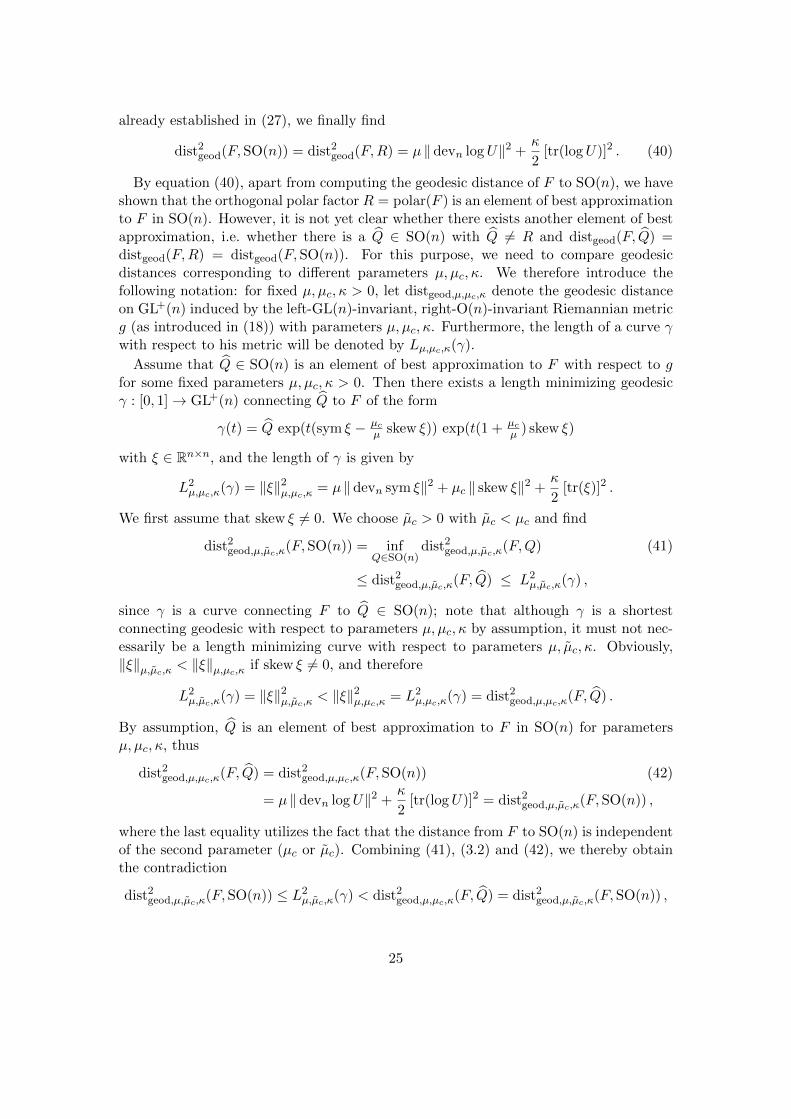
already established in (27), we finally find

dist2geod(F,SO(n)) = dist2

geod(F,R) = µ ‖ devn logU‖2 +κ

2[tr(logU)]2 . (40)

By equation (40), apart from computing the geodesic distance of F to SO(n), we haveshown that the orthogonal polar factor R = polar(F ) is an element of best approximationto F in SO(n). However, it is not yet clear whether there exists another element of bestapproximation, i.e. whether there is a Q ∈ SO(n) with Q 6= R and distgeod(F, Q) =distgeod(F,R) = distgeod(F,SO(n)). For this purpose, we need to compare geodesicdistances corresponding to different parameters µ, µc, κ. We therefore introduce thefollowing notation: for fixed µ, µc, κ > 0, let distgeod,µ,µc,κ denote the geodesic distanceon GL+(n) induced by the left-GL(n)-invariant, right-O(n)-invariant Riemannian metricg (as introduced in (18)) with parameters µ, µc, κ. Furthermore, the length of a curve γwith respect to his metric will be denoted by Lµ,µc,κ(γ).

Assume that Q ∈ SO(n) is an element of best approximation to F with respect to gfor some fixed parameters µ, µc, κ > 0. Then there exists a length minimizing geodesicγ : [0, 1]→ GL+(n) connecting Q to F of the form

γ(t) = Q exp(t(sym ξ − µcµ skew ξ)) exp(t(1 + µc

µ ) skew ξ)

with ξ ∈ Rn×n, and the length of γ is given by

L2µ,µc,κ(γ) = ‖ξ‖2µ,µc,κ = µ ‖ devn sym ξ‖2 + µc ‖ skew ξ‖2 +

κ

2[tr(ξ)]2 .

We first assume that skew ξ 6= 0. We choose µc > 0 with µc < µc and find

dist2geod,µ,µc,κ(F,SO(n)) = inf

Q∈SO(n)dist2

geod,µ,µc,κ(F,Q) (41)

≤ dist2geod,µ,µc,κ(F, Q) ≤ L2

µ,µc,κ(γ) ,

since γ is a curve connecting F to Q ∈ SO(n); note that although γ is a shortestconnecting geodesic with respect to parameters µ, µc, κ by assumption, it must not nec-essarily be a length minimizing curve with respect to parameters µ, µc, κ. Obviously,‖ξ‖µ,µc,κ < ‖ξ‖µ,µc,κ if skew ξ 6= 0, and therefore

L2µ,µc,κ(γ) = ‖ξ‖2µ,µc,κ < ‖ξ‖

2µ,µc,κ

= L2µ,µc,κ(γ) = dist2

geod,µ,µc,κ(F, Q) .

By assumption, Q is an element of best approximation to F in SO(n) for parametersµ, µc, κ, thus

dist2geod,µ,µc,κ(F, Q) = dist2

geod,µ,µc,κ(F,SO(n)) (42)

= µ ‖devn logU‖2 +κ

2[tr(logU)]2 = dist2

geod,µ,µc,κ(F,SO(n)) ,

where the last equality utilizes the fact that the distance from F to SO(n) is independentof the second parameter (µc or µc). Combining (41), (3.2) and (42), we thereby obtainthe contradiction

dist2geod,µ,µc,κ(F,SO(n)) ≤ L2

µ,µc,κ(γ) < dist2geod,µ,µc,κ(F, Q) = dist2

geod,µ,µc,κ(F,SO(n)) ,

25

hence we must have skew ξ = 0. But then

γ(1) = Q exp(sym ξ − µcµ skew ξ) exp((1 + µc

µ ) skew ξ) = Q exp(sym ξ) ,

and since exp(sym ξ) ∈ PSym(n), the uniqueness of the polar decomposition F = RUyields exp(sym ξ) = U and, finally, Q = R.

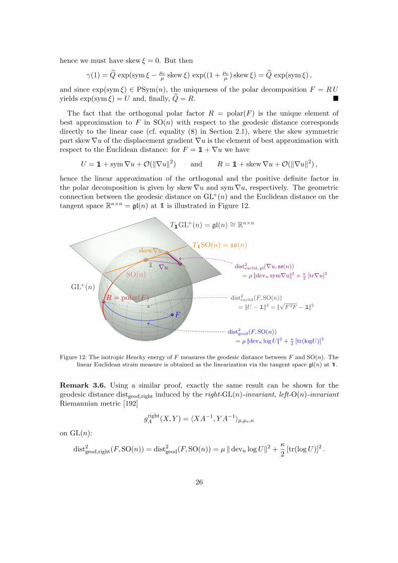
The fact that the orthogonal polar factor R = polar(F ) is the unique element ofbest approximation to F in SO(n) with respect to the geodesic distance correspondsdirectly to the linear case (cf. equality (8) in Section 2.1), where the skew symmetricpart skew∇u of the displacement gradient ∇u is the element of best approximation withrespect to the Euclidean distance: for F = 1+∇u we have

U = 1+ sym∇u+O(‖∇u‖2) and R = 1+ skew∇u+O(‖∇u‖2) ,

hence the linear approximation of the orthogonal and the positive definite factor inthe polar decomposition is given by skew∇u and sym∇u, respectively. The geometricconnection between the geodesic distance on GL+(n) and the Euclidean distance on thetangent space Rn×n = gl(n) at 1 is illustrated in Figure 12.

SO(n)

1

R = polar(F )

GL+(n)

T1GL+(n) = gl(n) ∼= Rn×n

T1SO(n) = so(n)

F

∇u

skew∇u

dist2euclid, gl(∇u, so(n))

= µ ||devn sym∇u||2 + κ2

[tr∇u]2

dist2euclid(F,SO(n))

= ||U − 1||2 = ||√FTF − 1||2

dist2geod(F,SO(n))

= µ ||devn logU ||2 + κ2

[tr(logU)]2

Figure 12: The isotropic Hencky energy of F measures the geodesic distance between F and SO(n). Thelinear Euclidean strain measure is obtained as the linearization via the tangent space gl(n) at 1.

Remark 3.6. Using a similar proof, exactly the same result can be shown for thegeodesic distance distgeod,right induced by the right-GL(n)-invariant, left-O(n)-invariantRiemannian metric [192]

grightA (X,Y ) = 〈XA−1, Y A−1〉µ,µc,κ

on GL(n):

dist2geod,right(F,SO(n)) = dist2

geod(F,SO(n)) = µ ‖ devn logU‖2 +κ

2[tr(logU)]2 .

26

B

F1 F1

F2 F2

Ω B · Ω

F1 · Ω F1 ·B · Ω

F2 · Ω F2 ·B · Ω

distgeod(F1, F2) distgeod(F1 ·B,F2 ·B)=

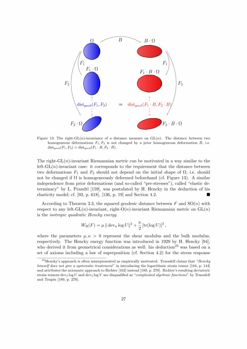
Figure 13: The right-GL(n)-invariance of a distance measure on GL(n): The distance between twohomogeneous deformations F1, F2 is not changed by a prior homogeneous deformation B, i.e.distgeod(F1, F2) = distgeod(F1 ·B,F2 ·B).

The right-GL(n)-invariant Riemannian metric can be motivated in a way similar to theleft-GL(n)-invariant case: it corresponds to the requirement that the distance betweentwo deformations F1 and F2 should not depend on the initial shape of Ω, i.e. shouldnot be changed if Ω is homogeneously deformed beforehand (cf. Figure 13). A similarindependence from prior deformations (and so-called “pre-stresses”), called “elastic de-terminacy” by L. Prandtl [159], was postulated by H. Hencky in the deduction of hiselasticity model; cf. [93, p. 618], [136, p. 19] and Section 4.2.

According to Theorem 3.3, the squared geodesic distance between F and SO(n) withrespect to any left-GL(n)-invariant, right-O(n)-invariant Riemannian metric on GL(n)is the isotropic quadratic Hencky energy

WH(F ) = µ ‖ devn logU‖2 +κ

2[tr(logU)]2 ,

where the parameters µ, κ > 0 represent the shear modulus and the bulk modulus,respectively. The Hencky energy function was introduced in 1929 by H. Hencky [94],who derived it from geometrical considerations as well: his deduction23 was based on aset of axioms including a law of superposition (cf. Section 4.2) for the stress response

23Hencky’s approach is often misrepresented as empirically motivated. Truesdell claims that “Henckyhimself does not give a systematic treatement” in introducing the logarithmic strain tensor [184, p. 144]and attributes the axiomatic approach to Richter [162] instead [189, p. 270]. Richter’s resulting deviatoricstrain tensors dev3 logU and dev3 log V are disqualified as “complicated algebraic functions” by Truesdelland Toupin [189, p. 270].

27

function [136], an approach previously employed by G.F. Becker [19, 145] in 1893 andlater followed in a more general context by H. Richter [162], cf. [163, 161, 164]. A differentconstitutive model for uniaxial deformations based on logarithmic strain had previouslybeen proposed by Imbert [106] and Hartig [82]. While Ludwik is often credited withthe introduction of the uniaxial logarithmic strain, his ubiquitously cited article [115](which is even referenced by Hencky himself [95, p. 175]) does not provide a systematicintroduction of such a strain measure.

While the energy function WH(F ) = dist2geod(F,SO(n)) already defines a measure of

strain as described in Section 1.1, we are also interested in characterizing the two terms‖ devn logU‖ and | tr(logU)| as separate partial strain measures.

Theorem 3.7 (Partial strain measures). Let

ωiso(F ) := ‖ devn log√F TF‖ and ωvol(F ) := | tr(log

√F TF )| .

Then

ωiso(F ) = distgeod, SL(n)

(F

detF 1/n, SO(n)

)

and

ωvol(F ) =√n · distgeod,R+·1

((detF )1/n · 1, 1

),

where the geodesic distances distgeod, SL(n) and distgeod,R+·1 on the Lie groups SL(n) =A ∈ GL(n) | detA = 1 and R+ · 1 are induced by the canonical left-invariant metric

gA(X,Y )1 = 〈A−1X,A−1Y 〉 = tr(XTA−TA−1Y ) .

Remark 3.8. Theorem 3.7 states that ωiso and ωvol appear as natural measures ofthe isochoric and volumetric strain, respectively: if F = Fiso Fvol is decomposed mul-tiplicatively [66] into an isochoric part Fiso = (detF )−1/n · F and a volumetric partFvol = (detF )1/n ·1, then ωiso(F ) measures the SL(n)-geodesic distance of Fiso to SO(n),whereas 1√

nωvol(F ) gives the geodesic distance of Fvol to the identity 1 in the group

R+ · 1 of purely volumetric deformations.

Proof. First, observe that the canonical left-invariant metrics on SL(n) and R+ · 1 areobtained by choosing µ = µc = 1 and κ = 2

n and restricting the corresponding metric gon GL+(n) to the submanifolds SL(n), R+ ·1 and their respective tangent spaces. Thenfor this choice of parameters, every curve in SL(n) or R+ · 1 is a curve of equal lengthin GL+(n) with respect to g. Since the geodesic distance is defined as the infimal lengthof connecting curves, this immediately implies

distgeod, SL(n) (Fiso, SO(n)) ≥ distgeod,GL+(n) (Fiso, SO(n))

as well as

distgeod,R+·1 (Fvol, 1) ≥ distgeod,GL+(n) (Fvol, 1) ≥ distgeod,GL+(n) (Fvol, SO(n))

28

for Fiso := (detF )−1/n · F and Fvol := (detF )1/n · 1. We can therefore use Theorem 3.3to obtain the lower bounds24

dist2geod, SL(n) (Fiso, SO(n))

≥ dist2geod,GL+(n) (Fiso, SO(n))

= ‖ devn log

(√F TisoFiso

)‖2 +

1

n

[tr

(log√F TisoFiso

)]2

= ‖ log

((det√F TisoFiso

)−1/n√F TisoFiso

)‖2 +

1

n

[ln

( =1︷︸︸︷det√F TisoFiso

)]2

= ‖ log

(√F TisoFiso

)‖2 = ‖ log

((detF )−1/n

√F TF

)‖2 = ω2

iso(F ) (43)

and

dist2geod,R+·1 (Fvol, 1) ≥ dist2

geod,GL+(n) (Fvol, SO(n))

= ‖ devn log

(√F TvolFvol

)‖2 +

1

n[tr(log

(√F TvolFvol

))]2 (44)

= ‖ devn

(ln((detF )1/n) · 1

)‖2 +

1

n[ln(det

((detF )1/n · 1

))]2

=1

n[ln(det

√F TF )]2 =

1

n[tr(log

√F TF )]2 =

1

nω2

vol(F ) .

To obtain an upper bound on the geodesic distances, we define the two curves

γiso : [0, 1]→ SL(n) , γiso(t) = R exp(t devn logU)

and

γvol : [0, 1]→ R+ · 1 , γvol(t) = etn

tr(logU) · 1 ,

where F = RU with R ∈ SO(n) and U ∈ PSym(n) is the polar decomposition of F .Then γiso connects (detF )−1/n · F to SO(n):

γiso(0) = R ∈ SO(n) ,

γiso(1) = R exp(devn logU) = R exp(logU − tr(logU)n · 1)

= R exp(logU) exp(− tr(logU)n · 1)

= RU exp(− ln detUn · 1) = (detU)−1/n · F = (detF )−1/n · F ,

while γvol connects (detF )1/n · 1 and 1:

γvol(0) = 1 , γvol(1)= e1n

tr(logU) · 1 = e1n

ln(detU) · 1 = (detU)1/n · 1 = (detF )1/n · 1 .24For some of the rules of computation employed here involving the matrix logarithm, we refer to

Lemma A.1 in the appendix.

29

The lengths of the curves compute to

L(γiso) =

∫ 1

0‖γiso(t)−1γiso(t)‖dt (45)

=

∫ 1

0‖(R exp(t devn logU))−1R exp(t devn logU) devn logU‖ dt

=

∫ 1

0‖ devn logU‖ dt = ‖ devn log

√F TF‖ = ωiso(F )

as well as

L(γvol) =

∫ 1

0‖γvol(t)

−1γvol(t)‖ dt (46)

=

∫ 1

0‖(e tn tr(logU) · 1)−1 · tr(logU)

n · e tn tr(logU) · 1‖ dt

=

∫ 1

0‖ tr(logU)

n · 1‖ dt =| tr(logU)|

n· ‖1‖ =

1√n| tr(log

√F TF )| = 1√

nωvol(F ) ,

showing that

dist2geod, SL(n)

((detF )−1/n · F, SO(n)

)≤ L2(γiso) = ω2

iso(F )

and

dist2geod,R+·1

((detF )1/n · 1, 1

)≤ L2(γvol) =

1

n· ω2

vol(F ) ,

which completes the proof.

Remark 3.9. In addition to the isochoric (distortional) part Fiso = (detF )−1/n · F andthe volumetric part Fvol = (detF )1/n · 1, we may also consider the cofactor Cof F =(detF ) · F−T of F ∈ GL+(n). Theorem 3.3 allows us to directly compute (cf. AppendixA.4) the distance

dist2geod(Cof F,SO(n)) = µ ‖ devn logU‖2 +

κ (n− 1)2

2[tr(logU)]2 .

4. Alternative motivations for the logarithmic strain

4.1. Riemannian geometry applied to PSym(n)

Extensive work on the use of Lie group theory and differential geometry in continuummechanics has already been done by Rougee [166, 165, 167, 168], Moakher [128], Bhatia[28] and, more recently, by Fiala [58, 59, 60, 61] (cf. [111]). They all endowed the convexcone PSym(3) of positive definite symmetric (3×3)-tensors with the Riemannian metric25

gC(X,Y ) = tr(C−1XC−1Y ) = 〈XC−1, C−1Y 〉 = 〈C−1/2X C−1/2, C−1/2 Y C−1/2〉 , (47)

25Note the subtle difference to our metric gC(X,Y ) = 〈C−1X,C−1Y 〉.

30

where C ∈ PSym(3) and X,Y ∈ Sym(3) = TC PSym(3). Fiala and Rougee deduceda motivation of the logarithmic strain tensor logU via geodesic curves connecting el-ements of PSym(n). However, their approach differs markedly from our method em-ployed in the previous sections: the manifold PSym(n) already corresponds to metricstates C = F TF , whereas we consider the full set GL+(n) of deformation gradients F(cf. Appendix A.3 and Table 1 in Section 6). This restriction can be viewed as thenonlinear analogue of the a priori restriction to ε = sym∇u in the linear case, i.e. thenature of the strain measure is not deduced but postulated. Note also that the metric gcannot be obtained by restricting our left-GL(3)-invariant, right-O(3)-invariant metric gto PSym(3).26 Furthermore, while Fiala and Rougee aim to motivate the Hencky straintensor logU directly, our focus lies on the strain measures ωiso, ωvol and the isotropicHencky strain energy WH.

The geodesic curves on PSym(n) with respect to g are of the simple form27

γ(t) = C1/21 exp(t · C−1/2

1 M C−1/21 )C

1/21 (48)

with C1 ∈ PSym(n) and M ∈ Sym(n) = T1 PSym(n). These geodesics are defined glob-ally, i.e. PSym(n) is geodesically complete. Furthermore, for given C1, C2 ∈ PSym(n),there exists a unique geodesic curve connecting them; this easily follows from the repre-sentation formula (48) or from the fact that the curvature of PSym(n) with g is constantand negative [59, 108, 27]. Note that this implies that, in contrast to GL+(n) with ourmetric g, there are no closed geodesics on PSym(n).

An explicit formula for the corresponding geodesic distance was given by Moakher:28

distgeod,PSym(n)(C1, C2) = ‖ log(C−1/22 C1C

−1/22 )‖ . (49)

In the special case C2 = 1, this distance measure is equal to our geodesic distance onGL+(n) induced by the canonical inner product: Theorem 3.3, applied with parametersµ = µc = 1 and κ = 2

n to R = 1 and U = C1, shows that

distgeod,GL+(n)(C1,1) = ‖ logC1‖ = distgeod,PSym(n)(C1,1) .

More generally, assume that the two metric states C1, C2 ∈ PSym(n) commute. Then

26Since PSym(n) is not a Lie group with respect to matrix multiplication, the metric g itself cannotbe left- or right-invariant in any suitable sense.

27While Moakher gives the parametrization stated here, Rougee writes the geodesics in the formγ(t) = exp(t ·Log(C2C

−11 ))C1 with C1, C2 ∈ PSym(n), which can also be written as γ(t) = (C2C

−11 )t C1;

a similar formulation is given by Tarantola [182, (2.78)]. For a suitable definition of a matrix logarithm

Log on GL+(n), these representations are equivalent to (48) with M = log(C−1/22 C1 C

−1/22 ).

28Moakher [128, (2.9)] writes this result as ‖Log(C−12 C1)‖ =

√∑ni=1 ln2 λi, where λi are the (real

and positive) eigenvalues of C−12 C1. The right hand side of this equation is identical to the result stated

in (49). However, since C−12 C1 is not necessarily normal, there is in general no logarithm Log(C−1

2 C1)whose Frobenius norm satisfies this equality.

31

C−12 C1 ∈ PSym(n), and the left-GL(n)-invariance of the geodesic distance implies

distgeod,GL+(n)(C1, C2) = distgeod,GL+(n)(C−12 C1,1) = ‖ log(C−1

2 C1)‖= ‖ log(C

−1/22 C

−1/22 C1)‖ = ‖ log(C

−1/22 C1C

−1/22 )‖ (50)

= distgeod,PSym(n)(C1, C2) .

However, since C−12 C1 /∈ PSym(n) in general, this equality does not hold on all of

PSym(n).A different approach towards distance functions on the set PSym(n) was suggested

by Arsigny et al. [8, 9, 7] who, motivated by applications of geodesic and logarith-mic distances in diffusion tensor imaging, directly define their Log-Euclidean metric onPSym(n) by

distLog-Euclid(C1, C2) := ‖ logC1 − logC2‖ , (51)

where ‖ . ‖ is the Frobenius matrix norm. If C1 and C2 commute, this distance equalsthe geodesic distance on GL+(n) as well:

distgeod,GL+(n)(C1, C2) = ‖ log(C−12 C1)‖

= ‖ log(C−12 ) + log(C1)‖ (52)

= ‖ logC1 − logC2‖ = distLog-Euclid(C1, C2) ,

where equality in (52) holds due to the fact that C1 and C−12 commute. Again, this

equality does not hold for arbitrary C1 and C2.Using a similar Riemannian metric, geodesic distance measures can also be applied

to the set of positive definite symmetric fourth-order elasticity tensors, which can beidentified with PSym(6). Norris and Moakher applied such a distance function in orderto find an isotropic elasticity tensor C : Sym(3) → Sym(3) which best approximates agiven anisotropic tensor [129, 147].

The connection between geodesic distances on the metric states in PSym(n) and loga-rithmic distance measures was also investigated extensively by the late Albert Tarantola[182], a lifelong advocate of logarithmic measures in physics. In his view [182, 4.3.1],“. . . the configuration space is the Lie group GL+(3), and the only possible measure ofstrain (as the geodesics of the space) is logarithmic.”

4.2. Further mechanical motivations for the quadratic isotropic Henckymodel based on logarithmic strain tensors

“At the foundation of all elastic theories lies the definition of strain, andbefore introducing a new law of elasticity we must explain how finite strainis to be measured.”

Heinrich Hencky: The elastic behavior of vulcanized rubber [96].

Apart from the geometric considerations laid out in the previous sections, the Henckystrain tensor E0 = logU can be characterized via a number of unique properties.

32

For example, the Hencky strain is the only strain tensor (for a suitably narrow defini-tion, cf. [145]) that satisfies the law of superposition for coaxial deformations:

E0(U1 · U2) = E0(U1) + E0(U2) (53)

for all coaxial stretches U1 and U2, i.e. U1, U2 ∈ PSym(n) such that U1 ·U2 = U2 ·U1. Thischaracterization was used by Heinrich Hencky [181, 90, 95, 96] in his original introductionof the logarithmic strain tensor [92, 94, 93, 136] and, indeed much earlier, by the geologistGeorge Ferdinand Becker [124], who postulated a similar law of superposition in orderto deduce a logarithmic constitutive law of nonlinear elasticity [19, 145] (cf. AppendixA.2).

In the case n = 1, this superposition principle simply amounts to the fact that thelogarithm function f = log satisfies Cauchy’s [38] well-known functional equation

f(λ1 · λ2) = f(λ1) + f(λ2) . (54)

This means that for a sequence of incremental one-dimensional deformations, the loga-rithmic strains eilog can be added in order to obtain the total logarithmic strain etot

log ofthe composed deformation [65]:

e1log + e2

log + . . .+ enlog = logL1

L0+ log

L2

L1+ . . .+ log

LnLn−1

= logLnL0

= etotlog ,

where Li denotes the length of the (one-dimensional) body after the i-th elongation.This property uniquely characterizes the logarithmic strain elog among all differentiableone-dimensional strain mappings e : R+ → R with e′(1) = 1.

Since purely volumetric deformations of the form λ ·1 with λ > 0 are coaxial to everystretch U ∈ PSym(n), the decomposition property (53) allows for a simple additivevolumetric-isochoric split of the Hencky strain tensor [162]:

logU = log

[U

(detU)1/n

︸︷︷︸isochoric

· (detU)1/n · 1︸︷︷︸

volumetric

]= devn logU

︸︷︷︸isochoric

+1

ntr(logU) · 1

︸︷︷︸volumetric

.

In particular, the incompressibility condition detF = 1 can be easily expressed astr(logU) = 0 in terms of the logarithmic strain.

4.2.1. From Truesdell’s hypoelasticity to Hencky’s hyperelastic model

As indicated in Section 1.1, the quadratic Hencky energy is also of great importance tothe concept of hypoelasticity [76, Chapter IX]. It was found that the Truesdell equation29

[184, 186, 185, 69]

d

dt

[τ ] = 2µD + λ tr(D) · 1 , D = sym(F F−1) , (55)

29It is telling to see that equation (55) had already been proposed by Hencky himself in [93] forthe Zaremba-Jaumann stress rate (cf. (58)). Hencky’s work, however, contains a typographical error[93, eq. (10) and eq. (11e)] changing the order of indices in his equations (cf. [33]). The strong point ofwriting (55) is that no discussion of any suitable strain tensor is necessary.

33

with constant coefficients µ, λ > 0, under the assumption that the stress rate ddt

is

objective30 and corotational, is satisfied if and only if ddt

is the so-called logarithmic

corotational rate ddt

logand τ = 2µ log V + λ tr(log V ) · 1 [196, 194, 148], i.e. if and

only if the hypoelastic model is exactly Hencky’s hyperelastic constitutive model. Here,τ = detF ·σ(V ) denotes the Kirchhoff stress tensor and D is the unique rate of stretchingtensor (i.e. the symmetric part of the velocity gradient in the spatial setting). A rateddt

is called corotational if it is of the special form

d

dt

[X] = X − ΩX +XΩ with Ω ∈ so(3) ,

which means that the rate is computed with respect to a frame that is rotated.31 Thisextra rate of rotation is defined only by the underlying spins of the problem. Uponspecialisation, for µ = 1, λ = 0 we obtain32 [32, eq. 71]

d

dt

log

[log V ] = D

as the unique solution to (55) with a corotational rate. Note that this characterizationof the spatial logarithmic strain tensor log V is by no means exceptional. For example,it is well known that [83, p. 49, Theorem 1.8] (cf. [34])

d

dt

M

[A] = A+ LTA+AL = D ,

where A = E−1 = 12(1−B−1) is the spatial Almansi strain tensor and d

dt

Mis the upper

Oldroyd rate (as defined in (59)).The quadratic Hencky model

τ = 2µ log V + λ tr(log V ) · 1 = Dlog VWH(log V ) (56)

was generalized in Hill’s generalized linear elasticity laws33 [132]

Tr = 2µEr + λ tr(Er) · 1 (57)

30A rate ddt

is called objective if d

dt

[S(QBQT )

]= Q ( d

dt

[S(B)])QT for all (not necessarily constant)

Q = Q(t) ∈ O(n), where S is any objective stress tensor, and if ddt

[S] = 0 ⇔ S = 0, i.e. the motion is

rigid if and only if ddt

[S] ≡ 0.

31Corotational rates are also special cases of Lie derivatives [118].32Cf. Xiao, Bruhns and Meyers [195, p. 90]: “. . . the logarithmic strain [does] possess certain intrinsic

far-reaching properties [which] establish its favoured position in all possible strain measures”.33Hooke’s law [103] (cf. [131]) famously states that the strain in a deformation depends linearly on

the occurring stress (“ut tensio, sic vis”). However, for finite deformations, different constitutive lawsof elasticity can be obtained from this assumption, depending on the choice of a stress/strain pair. Anidealized version of such a linear relation is given by (56), i.e. by choosing the spatial Hencky straintensor log V and the Kirchhoff stress tensor τ . Since, however, Hooke speaks of extension versus force,the correct interpretation of Hooke’s law is TBiot = 2µ (U − 1) + λ tr(U − 1) · 1, i.e. the case r = 1

2in

(57).

34

with work-conjugate pairs (Tr, Er) based on the Lagrangian strain measures given in (3);cf. Appendix A.2 for examples. The concept of work-conjugacy was introduced by Hillvia an invariance requirement; the spatial stress power must be equal to its Lagrangiancounterpart:

detF · 〈σ,D〉 = 〈Tr, Er〉 ,by means of which a material stress tensor is uniquely linked to its (material rate) conju-gate strain tensor. Hence it generalizes the virtual work principle and is the foundationof derived methods like the finite element method.

For the case of isotropic materials, Hoger [102] shows by spectral decomposition tech-niques that the work-conjugate stress to logU is the back-rotated Cauchy stress σ mul-tiplied by detF , hence 〈σ,D〉 = 〈RT σ R, d

dt logU〉, which is a generalization of Hill’searlier work [99, 101]. Sansour [170] additionally found that the Eshelby-like stress ten-sor Σ = CS2 is equally conjugate to logU ; here, S2 denotes the second Piola-Kirchhoffstress tensor. For anisotropy, however, the conjugate stress exists but follows a morecomplex format than for isotropy [102]. The logarithm of the left stretch log V in con-trast exhibits a work conjugate stress tensor only for isotropic materials, namely theKirchhoff stress tensor τ = detF · σ [152, 102].

While hyperelasticity in its potential format avoids rate equations, the use of stressrates (i.e. stress increments in time) may be useful for the description of inelastic materialbehavior at finite strains. Since the material time derivative of an Eulerian stress tensoris not objective, rates for a tensor X were developed, like the (objective and corotational)Zaremba-Jaumann rate

d

dt

[X] = X −WX +XW , W = skewL , L = FF−1 , (58)

or the (objective but not corotational) lower and upper Oldroyd rates

d

dt

O

[X] = X + LTX +XL andd

dt

M

[X] = X − LX −XLT , (59)

to name but a few (cf. [83, Section 1.7]). Which one of these or the great number ofother objective rates should be used seems to be rather a matter of taste, hence ofarbitrariness34 or heuristics35, but not a matter of theory.

The concept of dual variables36 as introduced by Tsakmakis and Haupt in [84] intocontinuum mechanics overcame the arbitrariness of the chosen rate in that it uniquelyconnects a particular (objective) strain rate to a stress tensor and, analogously, a stressrate to a strain tensor. The rational rule is that, when stress and strain tensors operateon configurations other than the reference configurations, the physically significant scalar

34Truesdell and Noll [188, p. 404] declared that “various such stress rates have been used in literature.Despite claims and whole papers to the contrary, any advantage claimed for one such rate over anotheris pure illusion.”

35For a shear test in Eulerian elasto-plasticity using the Zaremba-Jaumann rate (58), an unphysicalartefact of oscillatory shear stress was observed, first in [113]. A similar oscillatory behavior was observedfor hypoelasticity in [49].

36Hill [101] used the terms conjugate and dual as synonyms.

35

products 〈S2, E1〉, 〈S2, E1〉, 〈S2, E1〉 and 〈S2, E1〉 (with the second Piola-Kirchhoff stresstensor S2 and its work-conjugate Green strain tensor E1) must remain invariant, see[84, 83].

4.2.2. Advantageous properties of the quadratic Hencky energy

For modelling elastic material behavior there is no theoretical reason to prefer one straintensor over another one, and the same is true for stress tensors. As discussed in Section1.1, stress and strain are immaterial.37 Primary experimental data (forces, displace-ments) in material testing are sufficient to calculate any strain tensor and any stresstensor and to display any combination thereof in stress-strain curves, while only work-conjugate pairs are physically meaningful.

However, for modelling finite-strain elasticity, the quadratic Hencky model

WH = µ ‖devn log V ‖2 +κ

2[tr(log V )]2 = µ ‖ devn logU‖2 +

κ

2[tr(logU)]2 ,

τ = 2µ devn log V + κ tr(log V )1 , (60)

exhibits a number of unique, favorable properties, including its functional simplicity andits dependency on only two material parameters µ and κ that are determined in theinfinitesimal strain regime and remain constant over the entire strain range. In viewof the linear dependency of stress from logarithmic strain in (60), it is obvious thatany nonlinearity in the stress-strain curves can only be captured in Hencky’s modelby virtue of the nonlinearity in the strain tensor itself. There is a surprisingly largenumber of different materials, where Hencky’s elasticity relation provides a very goodfit to experimental stress-strain data, which is true for different length scales and strainregimes. In the following we substantiate this claim with some examples.

Nonlinear elasticity on macroscopic scales for a variety of materials. Anand [3, 4]has shown that the Hencky model is in good agreement with experiments on a wideclass of materials, e.g. vulcanized natural rubber, for principal stretches between 0.7and 1.3. More precisely, this refers to the characteristic that in tensile deformation thestiffness becomes increasingly smaller compared with the stiffness at zero strain, whilefor compressive deformation the stiffness becomes increasingly larger.

Nonlinear elasticity in the very small strain regime. We mention in passing that aqualitatively similar dependency of material stiffness on the sign of the strain has beenmade much earlier in the regime of extremely small strains (10−6–10−3). In Hartig’slaw [82] from 1893 this dependency was expressed as dσ

dε = E0 + b σ, where E0 is theelasticity modulus at zero stress and b < 0 is a dimensionless constant,38 cf. the book

37Cf. Truesdell [184, p. 145]: “It is important to realize that since each of the several material tensors[. . . ] is an isotropic function of any one of the others, an exact description of strain in terms of anyone is equivalent to a description in terms of any other” or Antman [6, p. 423]: “In place of C, anyinvertible tensor-valued function of C can be used as a measure of strain.”

38The negative curvature (b < 0) was already suggested by Jacob Bernoulli in 1705 [22] (cf. [21, p.276]): “Homogeneous fibers of the same length and thickness, but loaded with different weights, neitherlengthen nor shorten proportional to these weights; but the lengthening or the shortening caused by thesmall weight is less than the ratio that the first weight has to the second.”

36

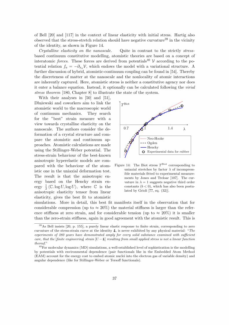
of Bell [20] and [117] in the context of linear elasticity with initial stress. Hartig alsoobserved that the stress-stretch relation should have negative curvature39 in the vicinityof the identity, as shown in Figure 14.

Crystalline elasticity on the nanoscale. Quite in contrast to the strictly stress-based continuum constitutive modelling, atomistic theories are based on a concept ofinteratomic forces. These forces are derived from potentials40 V according to the po-tential relation fa = −∂xaV, which endows the model with a variational structure. Afurther discussion of hybrid, atomistic-continuum coupling can be found in [54]. Therebythe discreteness of matter at the nanoscale and the nonlocality of atomic interactionsare inherently captured. Here, atomistic stress is neither a constitutive agency nor doesit enter a balance equation. Instead, it optionally can be calculated following the virialstress theorem [180, Chapter 8] to illustrate the state of the system.

0.7 1 1.4 λ

TBiot

Neo-Hooke

Ogden

HenckyExperimental data for rubber

Figure 14: The Biot stress TBiot corresponding touniaxial stretches by factor λ of incompress-ible materials fitted to experimental measure-ments by Jones and Treloar [107]. The cur-vature in λ = 1 suggests negative third orderconstants (b < 0), which has also been postu-lated by Grioli [77, eq. (32)].

With their analyses in [50] and [51],D luzewski and coworkers aim to link theatomistic world to the macroscopic worldof continuum mechanics. They searchfor the ”best” strain measure with aview towards crystalline elasticity on thenanoscale. The authors consider the de-formation of a crystal structure and com-pare the atomistic and continuum ap-proaches. Atomistic calculations are madeusing the Stillinger-Weber potential. Thestress-strain behaviour of the best-knownanisotropic hyperelastic models are com-pared with the behaviour of the atom-istic one in the uniaxial deformation test.The result is that the anisotropic en-ergy based on the Hencky strain en-ergy 1

2 〈C. logU, logU〉, where C is theanisotropic elasticity tensor from linearelasticity, gives the best fit to atomisticsimulations. More in detail, this best fit manifests itself in the observation that forconsiderable compression (up to ≈ 20%) the material stiffness is larger than the refer-ence stiffness at zero strain, and for considerable tension (up to ≈ 20%) it is smallerthan the zero-strain stiffness, again in good agreement with the atomistic result. This is

39As Bell insists [20, p. 155], a purely linear elastic response to finite strain, corresponding to zerocurvature of the stress-strain curve at the identity 1, is never exhibited by any physical material: “Theexperiments of 280 years have demonstrated amply for every solid substance examined with sufficientcare, that the [finite engineering] strain [U−1] resulting from small applied stress is not a linear functionthereof.”

40For molecular dynamics (MD) simulations, a well-established level of sophistication is the modellingby potentials with environmental dependence (pair functionals like in the Embedded Atom Method(EAM) account for the energy cost to embed atomic nuclei into the electron gas of variable density) andangular dependence (like for Stillinger-Weber or Tersoff functionals).

37

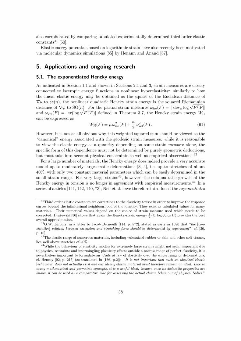
also corroborated by comparing tabulated experimentally determined third order elasticconstants41 [50].

Elastic energy potentials based on logarithmic strain have also recently been motivatedvia molecular dynamics simulations [85] by Henann and Anand [87].

5. Applications and ongoing research

5.1. The exponentiated Hencky energy

As indicated in Section 1.1 and shown in Sections 2.1 and 3, strain measures are closelyconnected to isotropic energy functions in nonlinear hyperelasticity: similarly to howthe linear elastic energy may be obtained as the square of the Euclidean distance of∇u to so(n), the nonlinear quadratic Hencky strain energy is the squared Riemanniandistance of ∇ϕ to SO(n). For the partial strain measures ωiso(F ) = ‖ devn log

√F TF‖

and ωvol(F ) = | tr(log√F TF )| defined in Theorem 3.7, the Hencky strain energy WH

can be expressed as

WH(F ) = µω2iso(F ) +

κ

2ω2

vol(F ) . (61)

However, it is not at all obvious why this weighted squared sum should be viewed as the“canonical” energy associated with the geodesic strain measures: while it is reasonableto view the elastic energy as a quantity depending on some strain measure alone, thespecific form of this dependence must not be determined by purely geometric deductions,but must take into account physical constraints as well as empirical observations.42

For a large number of materials, the Hencky energy does indeed provide a very accuratemodel up to moderately large elastic deformations [3, 4], i.e. up to stretches of about40%, with only two constant material parameters which can be easily determined in thesmall strain range. For very large strains43, however, the subquadratic growth of theHencky energy in tension is no longer in agreement with empirical measurements.44 In aseries of articles [141, 142, 140, 73], Neff et al. have therefore introduced the exponentiated

41Third order elastic constants are corrections to the elasticity tensor in order to improve the responsecurves beyond the infinitesimal neighbourhood of the identity. They exist as tabulated values for manymaterials. Their numerical values depend on the choice of strain measure used which needs to becorrected. D luzewski [50] shows that again the Hencky-strain energy 1

2〈C. logU, logU〉 provides the best

overall approximation.42G.W. Leibniz, in a letter to Jacob Bernoulli [114, p. 572], stated as early as 1690 that “the [con-

stitutive] relation between extension and stretching force should be determined by experiment”, cf. [20,p. 10].

43The elastic range of numerous materials, including vulcanized rubber or skin and other soft tissues,lies well above stretches of 40%.

44While the behaviour of elasticity models for extremely large strains might not seem important dueto physical restraints and intermingling plasticity effects outside a narrow range of perfect elasticity, it isnevertheless important to formulate an idealized law of elasticity over the whole range of deformations;cf. Hencky [92, p. 215] (as translated in [136, p.2]): “It is not important that such an idealized elastic[behaviour] does not actually exist and our ideally elastic material must therefore remain an ideal. Like somany mathematical and geometric concepts, it is a useful ideal, because once its deducible properties areknown it can be used as a comparative rule for assessing the actual elastic behaviour of physical bodies.”

38

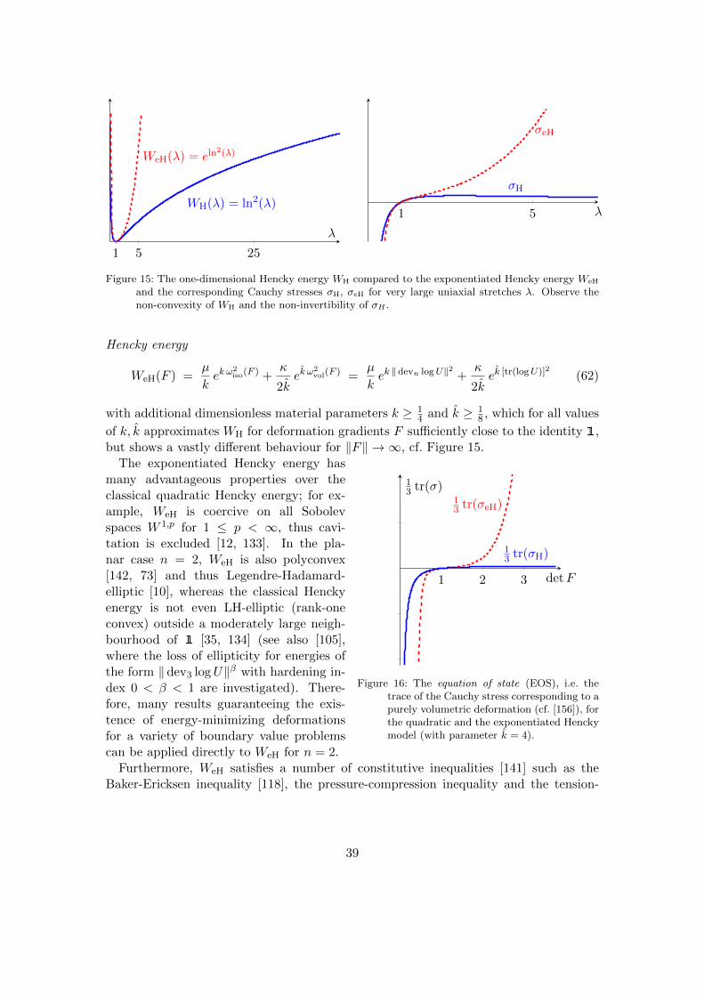
1 5 25

WH(λ) = ln2(λ)

WeH(λ) = eln2(λ)

λ

1 5

σH

σeH

λ

Figure 15: The one-dimensional Hencky energy WH compared to the exponentiated Hencky energy WeH

and the corresponding Cauchy stresses σH, σeH for very large uniaxial stretches λ. Observe thenon-convexity of WH and the non-invertibility of σH .

Hencky energy

WeH(F ) =µ

kek ω

2iso(F ) +

κ

2kek ω

2vol(F ) =

µ

kek ‖ devn logU‖2 +

κ

2kek [tr(logU)]2 (62)

with additional dimensionless material parameters k ≥ 14 and k ≥ 1

8 , which for all values

of k, k approximates WH for deformation gradients F sufficiently close to the identity 1,but shows a vastly different behaviour for ‖F‖ → ∞, cf. Figure 15.

1 2 3

13 tr(σeH)

13 tr(σH)

detF

13 tr(σ)

Figure 16: The equation of state (EOS), i.e. thetrace of the Cauchy stress corresponding to apurely volumetric deformation (cf. [156]), forthe quadratic and the exponentiated Henckymodel (with parameter k = 4).

The exponentiated Hencky energy hasmany advantageous properties over theclassical quadratic Hencky energy; for ex-ample, WeH is coercive on all Sobolevspaces W 1,p for 1 ≤ p < ∞, thus cavi-tation is excluded [12, 133]. In the pla-nar case n = 2, WeH is also polyconvex[142, 73] and thus Legendre-Hadamard-elliptic [10], whereas the classical Henckyenergy is not even LH-elliptic (rank-oneconvex) outside a moderately large neigh-bourhood of 1 [35, 134] (see also [105],where the loss of ellipticity for energies ofthe form ‖dev3 logU‖β with hardening in-dex 0 < β < 1 are investigated). There-fore, many results guaranteeing the exis-tence of energy-minimizing deformationsfor a variety of boundary value problemscan be applied directly to WeH for n = 2.

Furthermore, WeH satisfies a number of constitutive inequalities [141] such as theBaker-Ericksen inequality [118], the pressure-compression inequality and the tension-

39

extension inequality as well as Hill’s inequality45 [100, 150, 151], which is equivalent tothe convexity of the elastic energy with respect to the logarithmic strain tensor [177].

Moreover, for WeH, the Cauchy-stress-stretch relation V 7→ σeH(V ) is invertible (aproperty hitherto unknown for other hyperelastic formulations) and pure Cauchy shearstress corresponds to pure shear strain, as is the case in linear elasticity [141]. Thephysical meaning of Poisson’s ratio [157, 72] ν = 3κ−2µ

2(3κ+µ) is also similar to the linear

case; for example, ν = 12 directly corresponds to incompressibility of the material and

ν = 0 implies that no lateral extension or contraction occurs in uniaxial tensions tests.

5.2. Related geodesic distances

The logarithmic distance measures obtained in Theorems 3.3 and 3.7 show a strongsimilarity to other geodesic distance measures on Lie groups. For example, consider thespecial orthogonal group SO(n) endowed with the canonical bi-invariant Riemannianmetric46

gQ(X,Y ) = 〈QTX,QTY 〉 = 〈X,Y 〉for Q ∈ SO(n) and X,Y ∈ TQ SO(n) = Q · so(n). Then the geodesic exponential at1 ∈ SO(n) is given by the matrix exponential on the Lie algebra so(n), i.e. all geodesiccurves are one-parameter groups of the form

γ(t) = Q · exp(t A)

with Q ∈ SO(n) and A ∈ so(n) (cf. [127]). It is easy to show that the geodesic distancebetween Q,R ∈ SO(n) with respect to this metric is given by

distgeod, SO(n)(Q,R) = ‖ log(QTR)‖ ,

where ‖ . ‖ is the Frobenius matrix norm and log : SO(n)→ so(n) denotes the principalmatrix logarithm on SO(n), which is uniquely defined by the equality exp(logQ) = Qand the requirement λi(logQ) ∈ (−π, π] for all Q ∈ SO(n) and all eigenvalues λi(logQ).

This result can be extended to the geodesic distance on the conformal special orthog-onal group CSO(n) consisting of all angle-preserving linear mappings:

CSO(n) := c ·Q | c > 0 , Q ∈ SO(n) ,

where the bi-invariant metric gCSO(n) is given by the canonical inner product:

gCSO(n)A (X,Y ) = 〈A−1X,A−1Y 〉 . (63)

45Hill’s inequality [151] can be stated more generally as 〈 ddt

[τ ] − m [τ D − D τ ], D〉 ≥ 0 in the

hypoelastic formulation, where ddt

is the Zaremba-Jaumann stress rate (58) and τ is the Kirchhoff stress

tensor. For m = 0, as Silhavy explains, “Hill’s inequalities [. . . ] require the convexity of [the strainenergy W ] in [terms of the strain tensor log V ] . . . This does not seem to contradict any theoretical orexperimental evidence” [178, p. 309].

46Note that µc · g is the restriction of our left-GL(n)-invariant, right-O(n)-invariant metric g (asdefined in Section 3.1) to SO(n).

40

Then

dist2geod,CSO(n)(c ·Q, d ·R) = ‖ log(QTR)‖2 +

1

n

[ln( cd

)]2,

where log again denotes the principal matrix logarithm on SO(n). Note that the punc-tured complex plane C \ 0 can be identified with CSO(2) via the mapping

z = a+ i b 7→ Z ∈ CSO(2) =

(a b−b a

): a2 + b2 6= 0

.

5.3. Outlook

While first applications of the exponentiated Hencky energy, which is based on thepartial strain measures ωiso, ωvol introduced here, show promising results, including anaccurate modelling of so-called tire-derived material [130, 64], a more thorough fittingof the new parameter set to experimental data is necessary in order to assess the rangeof applicability of WeH towards elastic materials like vulcanized rubber. A differentformulation in terms of the partial strain measures ωiso and ωvol, i.e. an energy functionof the form

W (F ) = Ψ(ωiso(F ), ωvol(F )) = Ψ(‖ dev3 logU‖, |tr(logU)|) (64)

with Ψ : [0,∞)2 → [0,∞), might even prove to be polyconvex in the three-dimensionalcase. The main open problem of finding a polyconvex (or rank-one convex) isochoricenergy function47 F 7→ Ψ(‖dev3 logU‖) has also been considered by Sendova and Walton[173]. Note that while every isotropic elastic energy W can be expressed as W (F ) =h(K1,K2,K3) with Criscione’s invariants48 [44, 43, 48, 193]

K1 = tr(logU) , K2 = ‖ dev3 logU‖ and K3 = det

(dev3 logU

‖ dev3 logU‖

), (65)

not every elastic energy has a representation of the form (64); for example, (64) impliesthe tension-compression symmetry49 W (F ) = W (F−1), which is not necessarily satisfied

47Ideally, the function Ψ should also satisfy additional requirements, such as monotonicity, convexityand exponential growth.

48The invariants K1 and K22 = tr

[(dev3 logU)2

]as well as K3 = tr((dev3 logU)3) had already been

discussed exhaustively by H. Richter in a 1949 ZAMM article [162, §4], while K1 and K2 have also beenconsidered by A.I. Lurie [116, p. 189]. Criscione has shown that the invariants given in (65) enjoy afavourable orthogonality condition which is useful when determining material parameters.

49The tension-compression symmetry is often expressed as τ(V −1) = −τ(V ), where τ(V ) is theKirchhoff stress tensor corresponding to the left Biot stretch V . This condition, which is the naturalnonlinear counterpart of the equality σ(−ε) = −σ(ε) in linear elasticity, is equivalent to the conditionW (F−1) = W (F ) for hyperelastic constitutive models.

41

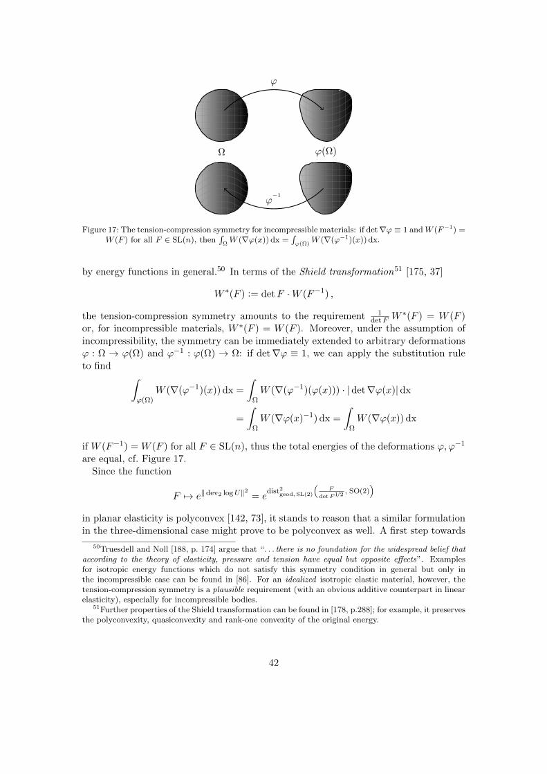
ϕ

Ω ϕ(Ω)

ϕ−1

Figure 17: The tension-compression symmetry for incompressible materials: if det∇ϕ ≡ 1 andW (F−1) =W (F ) for all F ∈ SL(n), then

∫ΩW (∇ϕ(x)) dx =

∫ϕ(Ω)

W (∇(ϕ−1)(x)) dx.

by energy functions in general.50 In terms of the Shield transformation51 [175, 37]

W ∗(F ) := detF ·W (F−1) ,

the tension-compression symmetry amounts to the requirement 1detF W

∗(F ) = W (F )or, for incompressible materials, W ∗(F ) = W (F ). Moreover, under the assumption ofincompressibility, the symmetry can be immediately extended to arbitrary deformationsϕ : Ω → ϕ(Ω) and ϕ−1 : ϕ(Ω) → Ω: if det∇ϕ ≡ 1, we can apply the substitution ruleto find

∫

ϕ(Ω)W (∇(ϕ−1)(x)) dx =

∫

ΩW (∇(ϕ−1)(ϕ(x))) · | det∇ϕ(x)|dx

=

∫

ΩW (∇ϕ(x)−1) dx =

∫

ΩW (∇ϕ(x)) dx

if W (F−1) = W (F ) for all F ∈ SL(n), thus the total energies of the deformations ϕ,ϕ−1

are equal, cf. Figure 17.Since the function

F 7→ e‖ dev2 logU‖2 = edist2

geod, SL(2)

(F

detF1/2, SO(2)

)

in planar elasticity is polyconvex [142, 73], it stands to reason that a similar formulationin the three-dimensional case might prove to be polyconvex as well. A first step towards

50Truesdell and Noll [188, p. 174] argue that “. . . there is no foundation for the widespread belief thataccording to the theory of elasticity, pressure and tension have equal but opposite effects”. Examplesfor isotropic energy functions which do not satisfy this symmetry condition in general but only inthe incompressible case can be found in [86]. For an idealized isotropic elastic material, however, thetension-compression symmetry is a plausible requirement (with an obvious additive counterpart in linearelasticity), especially for incompressible bodies.

51Further properties of the Shield transformation can be found in [178, p.288]; for example, it preservesthe polyconvexity, quasiconvexity and rank-one convexity of the original energy.

42

finding such an energy is to identify where the function W with

W (F ) = e‖ dev3 logU‖2 = edist2

geod, SL(3)

(F

detF1/3, SO(3)

), (66)

which is not rank-one convex [141], loses its ellipticity properties. For that purpose, itmay be useful to consider the quasiconvex hull of W . There already are a number ofpromising results for similar energy functions; for example, the quasiconvex hull of themapping

F 7→ dist2Euclid(F,SO(2)) = ‖U − 1‖2

can be explicitly computed [179], and the quasiconvex hull of the similar Saint-Venant-Kirchhoff energy WSVK(F ) = µ

4 ‖C − 1‖2 + λ8 [tr(C − 1)]2 has been given by Le Dret

and Raoult [112]. For the mappings

F 7→ dist2Euclid(F,SO(3)) or F 7→ dist2

geod(F,SO(n))

with n ≥ 2, however, no explicit representation of the quasiconvex hull is yet known,although it has been shown that both expressions are not rank-one convex [25].

It might also be of interest to calculate the geodesic distance distgeod(A,B) for alarger class of matrices A,B ∈ GL+(n):52 although Theorem 3.3 allows us to explicitlycompute the distance distgeod(1, P ) for P ∈ PSym(n) and local results are availablefor certain special cases [119], it is an open question whether there is a general formulafor the distance distgeod,GL+(n)(Q,R) between arbitrary rotations R,Q ∈ SO(n) for allparameters µ, µc, κ > 0. Since restricting our left-GL(n)-invariant, right-O(n)-invariantmetric on GL(n) to SO(n) yields a multiple of the canonical bi-SO(n)-invariant metricon SO(n), we can compute

dist2geod,GL+(n)(Q,R) = µc · dist2

geod,SO(n)(Q,R) = µc ‖ log(QTR)‖2

if for all Q,R ∈ SO(n) a shortest geodesic in GL+(n) connecting Q and R is alreadycontained within SO(n), cf. Figure 18. However, whether this is the case depends onthe chosen parameters µ, µc; a general closed-form solution for distgeod,GL+(n) on SO(n)is therefore not yet known [120].

Moreover, it is not known whether our result can be generalized to anisotropic Rie-mannian metrics, i.e. if the geodesic distance to SO(n) can be explicitly computed for alarger class of left-GL(n)-invariant Riemannian metrics which are not necessarily right-O(n)-invariant. A result in this direction would have immediate impact on the modellingof finite strain anisotropic elasticity [14, 171, 172]. The difficulties with such an exten-sion are twofold: one needs a representation formula for Riemannian metrics which areright-invariant under a given symmetry subgroup of O(n), as well as an understandingof the corresponding geodesic curves.

52An improved understanding of the geometric structure of mechanical problems could, for example,help to develop new discretization methods [169, 78].

43

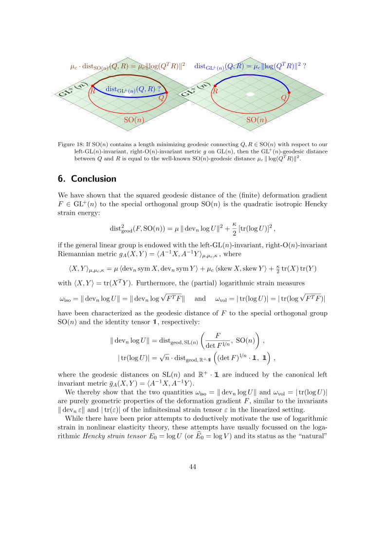
SO(n)

GL+(n

)

QR

µc · distSO(n)(Q,R) = µc‖log(QTR)‖2

distGL+(n)(Q,R) ?

distGL+(n)(Q,R) = µc‖log(QTR)‖2 ?

SO(n)

GL+(n

)

QR

µc · distSO(n)(Q,R) = µc‖log(QTR)‖2

distGL+(n)(Q,R) ?

distGL+(n)(Q,R) = µc‖log(QTR)‖2 ?

Figure 18: If SO(n) contains a length minimizing geodesic connecting Q,R ∈ SO(n) with respect to ourleft-GL(n)-invariant, right-O(n)-invariant metric g on GL(n), then the GL+(n)-geodesic distancebetween Q and R is equal to the well-known SO(n)-geodesic distance µc ‖ log(QTR)‖2.

6. Conclusion

We have shown that the squared geodesic distance of the (finite) deformation gradientF ∈ GL+(n) to the special orthogonal group SO(n) is the quadratic isotropic Henckystrain energy:

dist2geod(F,SO(n)) = µ ‖ devn logU‖2 +

κ

2[tr(logU)]2 ,

if the general linear group is endowed with the left-GL(n)-invariant, right-O(n)-invariantRiemannian metric gA(X,Y ) = 〈A−1X,A−1Y 〉µ,µc,κ , where

〈X,Y 〉µ,µc,κ = µ 〈devn symX,devn symY 〉+ µc 〈skewX, skew Y 〉+ κ2 tr(X) tr(Y )

with 〈X,Y 〉 = tr(XTY ). Furthermore, the (partial) logarithmic strain measures

ωiso = ‖ devn logU‖ = ‖devn log√F TF‖ and ωvol = | tr(logU)| = | tr(log

√F TF )|

have been characterized as the geodesic distance of F to the special orthogonal groupSO(n) and the identity tensor 1, respectively:

‖devn logU‖ = distgeod, SL(n)

(F

detF 1/n, SO(n)

),

| tr(logU)| = √n · distgeod,R+·1(

(detF )1/n · 1, 1),

where the geodesic distances on SL(n) and R+ · 1 are induced by the canonical leftinvariant metric gA(X,Y ) = 〈A−1X,A−1Y 〉.

We thereby show that the two quantities ωiso = ‖ devn logU‖ and ωvol = | tr(logU)|are purely geometric properties of the deformation gradient F , similar to the invariants‖ devn ε‖ and | tr(ε)| of the infinitesimal strain tensor ε in the linearized setting.

While there have been prior attempts to deductively motivate the use of logarithmicstrain in nonlinear elasticity theory, these attempts have usually focussed on the loga-rithmic Hencky strain tensor E0 = logU (or E0 = log V ) and its status as the “natural”

44

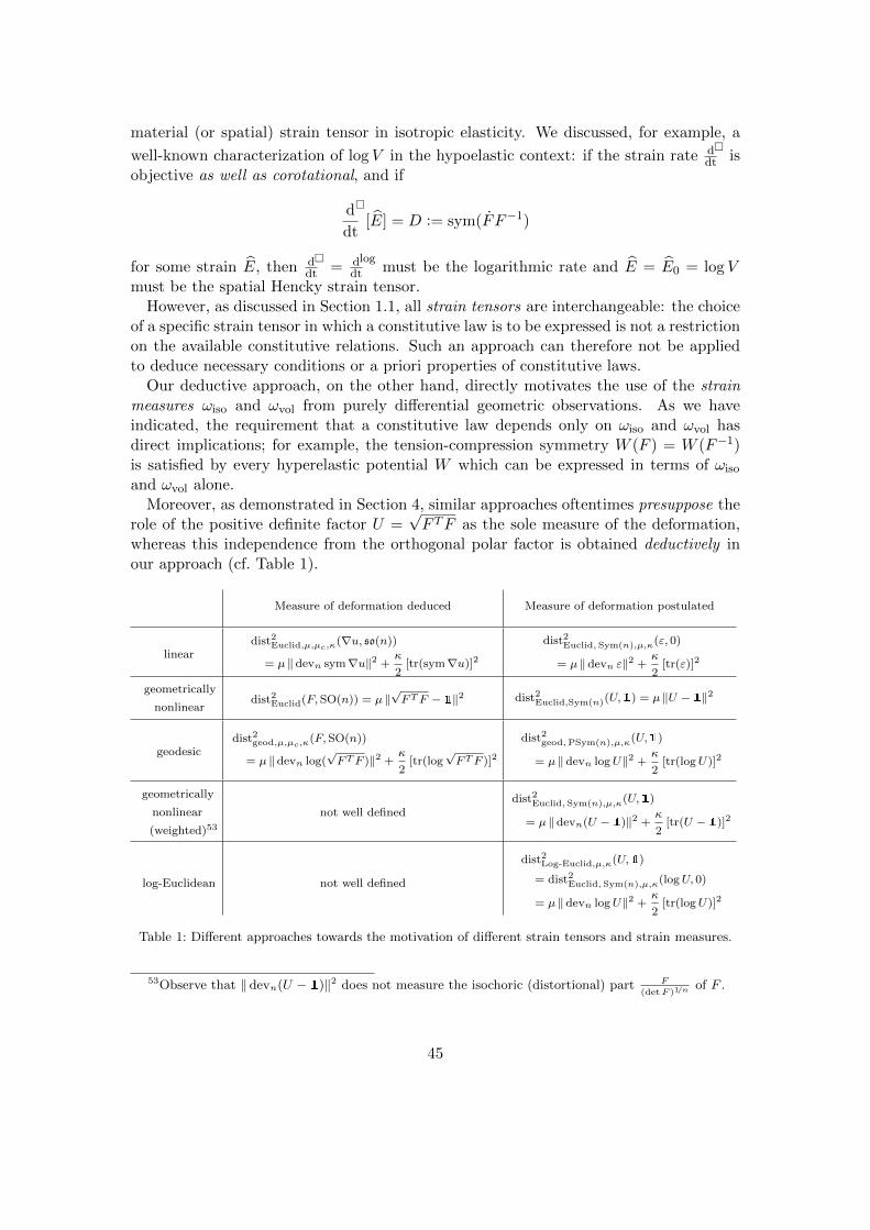
material (or spatial) strain tensor in isotropic elasticity. We discussed, for example, a

well-known characterization of log V in the hypoelastic context: if the strain rate ddt

is

objective as well as corotational, and if

d

dt

[E] = D := sym(FF−1)

for some strain E, then ddt

= d

dt

logmust be the logarithmic rate and E = E0 = log V

must be the spatial Hencky strain tensor.However, as discussed in Section 1.1, all strain tensors are interchangeable: the choice

of a specific strain tensor in which a constitutive law is to be expressed is not a restrictionon the available constitutive relations. Such an approach can therefore not be appliedto deduce necessary conditions or a priori properties of constitutive laws.

Our deductive approach, on the other hand, directly motivates the use of the strainmeasures ωiso and ωvol from purely differential geometric observations. As we haveindicated, the requirement that a constitutive law depends only on ωiso and ωvol hasdirect implications; for example, the tension-compression symmetry W (F ) = W (F−1)is satisfied by every hyperelastic potential W which can be expressed in terms of ωiso

and ωvol alone.Moreover, as demonstrated in Section 4, similar approaches oftentimes presuppose the

role of the positive definite factor U =√F TF as the sole measure of the deformation,

whereas this independence from the orthogonal polar factor is obtained deductively inour approach (cf. Table 1).

Measure of deformation deduced Measure of deformation postulated

lineardist2

Euclid,µ,µc,κ(∇u, so(n))

= µ ‖devn sym∇u‖2 +κ

2[tr(sym∇u)]2

dist2Euclid, Sym(n),µ,κ(ε, 0)

= µ ‖devn ε‖2 +κ

2[tr(ε)]2

geometrically

nonlineardist2

Euclid(F,SO(n)) = µ ‖√FTF − 1‖2 dist2

Euclid,Sym(n)(U,1) = µ ‖U − 1‖2

geodesicdist2

geod,µ,µc,κ(F,SO(n))

= µ ‖devn log(√FTF )‖2 +

κ

2[tr(log

√FTF )]2

dist2geod,PSym(n),µ,κ(U,1)

= µ ‖ devn logU‖2 +κ

2[tr(logU)]2

geometrically

nonlinear

(weighted)53

not well defineddist2

Euclid, Sym(n),µ,κ(U,1)

= µ ‖devn(U − 1)‖2 +κ

2[tr(U − 1)]2

log-Euclidean not well defined

dist2Log-Euclid,µ,κ(U,1)

= dist2Euclid, Sym(n),µ,κ(logU, 0)

= µ ‖ devn logU‖2 +κ

2[tr(logU)]2

Table 1: Different approaches towards the motivation of different strain tensors and strain measures.

53Observe that ‖ devn(U − 1)‖2 does not measure the isochoric (distortional) part F

(detF )1/nof F .

45

Note also that the specific distance measure distgeod on GL+(n) used here is not chosenarbitrarily: the requirements of left-GL(n)-invariance and right-O(n)-invariance, whichhave been motivated by mechanical considerations, uniquely determine g up to the threeparameters µ, µc, κ > 0. This uniqueness property further emphasizes the generality ofour results, which yet again strongly suggest that Hencky’s constitutive law should beconsidered the idealized nonlinear model of elasticity for very small strains outside theinfinitesimal range.

Acknowledgements

We are grateful to Prof. Alexander Mielke (Weierstraß-Institut, Berlin) for pertinentdiscussions on geodesics in GL(n); the first parametrization of geodesic curves on SL(n)known to us is due to him [125]. We also thank Prof. Robert Bryant (Duke Univer-sity) for his helpful remarks regarding geodesics on Lie groups and invariances of innerproducts on gl(n), as well as a number of friends who helped us with the draft.

We also thank Dr. Andreas Fischle (Rheinisch-Westfalische Technische HochschuleAachen) who, during long discussions on continuum mechanics and differential geometry,inspired many of the ideas laid out in this paper.

The first author had the great honour of presenting the main ideas of this paper toRichard Toupin on the occasion of the Canadian Conference on Nonlinear Solid Me-chanics 2013 in the mini-symposium organized by Francesco dell’Isola and David J.Steigmann, which was dedicated to Toupin.

References

[1] A.H. Al-Mohy, N.J. Higham, and S.D. Relton. Computing the Frechet derivative of the ma-trix logarithm and estimating the condition number. SIAM Journal on Scientific Computing,35(4):C394–C410, 2013.

[2] E. Almansi. Sulle deformazioni finite dei solidi elastici isotropi. Rendiconti della Reale Accademiadei Lincei, Classe di scienze fisiche, matematiche e naturali, 20, 1911.

[3] L. Anand. On H. Hencky’s approximate strain energy function for moderate deformations. Journalof Applied Mechanics, 46:78–82, 1979.

[4] L. Anand. Moderate deformations in extension-torsion of incompressible isotropic elastic materials.Journal of the Mechanics and Physics of Solids, 34:293–304, 1986.

[5] E. Andruchow, G. Larotonda, L. Recht, and A. Varela. The left invariant metric in the generallinear group. Journal of Geometry and Physics, 86(0):241 – 257, 2014.

[6] S.S. Antman. Nonlinear problems of elasticity, volume 107 of Applied Mathematical Sciences.Springer, New York, 2005.

[7] V. Arsigny, O. Commowick, N. Ayache, and X. Pennec. A fast and log-Euclidean polyaffineframework for locally linear registration. Journal of Mathematical Imaging and Vision, 33(2):222–238, 2009.

46

[8] V. Arsigny, P. Fillard, X. Pennec, and N. Ayache. Fast and simple calculus on tensors in the log-Euclidean framework. In Medical Image Computing and Computer-Assisted Intervention–MICCAI2005, pages 115–122. Springer, 2005.

[9] V. Arsigny, P. Fillard, X. Pennec, and N. Ayache. Geometric means in a novel vector space struc-ture on symmetric positive-definite matrices. SIAM Journal on Matrix Analysis and Applications,29(1):328–347, 2007.

[10] J.M. Ball. Convexity conditions and existence theorems in nonlinear elasticity. Archive for RationalMechanics and Analysis, 63(4):337–403, 1976.

[11] J.M. Ball. Constitutive inequalities and existence theorems in nonlinear elastostatics. In NonlinearAnalysis and Mechanics: Heriot-Watt Symposium, volume 1, pages 187–241. Pitman PublishingLtd. Boston, 1977.

[12] J.M. Ball. Discontinuous equilibrium solutions and cavitation in nonlinear elasticity. Philosoph-ical Transactions of the Royal Society of London. Series A, Mathematical and Physical Sciences,306(1496):557–611, 1982.

[13] J.M. Ball. Some open problems in elasticity. In Paul Newton, Philip Holmes, and Alan Weinstein,editors, Geometry, Mechanics, and Dynamics, pages 3–59. Springer, 2002.

[14] D. Balzani, P. Neff, J. Schroder, and G.A. Holzapfel. A polyconvex framework for soft biolog-ical tissues. Adjustment to experimental data. International Journal of Solids and Structures,43(20):6052–6070, 2006.

[15] R.C. Batra. Linear constitutive relations in isotropic finite elasticity. Journal of Elasticity,51(3):243–245, 1998.

[16] R.C. Batra. Comparison of results from four linear constitutive relations in isotropic finite elasticity.International Journal of Non-Linear Mechanics, 36(3):421–432, 2001.

[17] Z.P. Bazant. Easy-to-compute tensors with symmetric inverse approximating Hencky finite strainand its rate. Journal of Engineering Materials and Technology, 120(2):131–136, 1998.

[18] G.F. Becker. Finite Homogeneous Strain, Flow and Rupture of Rocks. Bulletin of the GeologicalSociety of America, 4:13–90, 1892.

[19] G.F. Becker. The Finite Elastic Stress-Strain Function. American Journal of Science, 46:337–356, 1893. newly typeset version available at https://www.uni-due.de/imperia/md/content/

mathematik/ag_neff/becker_latex_new1893.pdf.

[20] J.F. Bell and C. Truesdell. Mechanics of Solids: Volume 1: The Experimental Foundations of SolidMechanics. Handbuch der Physik. Springer, 1973.

[21] E. Benvenuto. An Introduction to the History of Structural Mechanics. Part I: Statics and Resis-tance of Solids. Springer, 1991.

[22] J. Bernoulli. Veritable hypothese de la resistance des solides, avec la demonstration de la courburedes corps qui font ressort. Memoires de l’Academie des Sciences, 1705.

[23] D.S. Bernstein. Matrix Mathematics: Theory, Facts, and Formulas (Second Edition). Princetonreference. Princeton University Press, 2009.

[24] A. Bertram. Elasticity and Plasticity of Large Deformations. Springer, 2008.

[25] A. Bertram, T. Bohlke, and M. Silhavy. On the rank 1 convexity of stored energy functions ofphysically linear stress-strain relations. Journal of Elasticity, 86(3):235–243, 2007.

47

https://www.uni-due.de/imperia/md/content/mathematik/ag_neff/becker_latex_new1893.pdf

https://www.uni-due.de/imperia/md/content/mathematik/ag_neff/becker_latex_new1893.pdf

[26] Y. Beygelzimer. Equivalent strain in simple shear deformations. available at arXiv:1301.1281,2013.

[27] R. Bhatia. Positive definite matrices. Princeton University Press, 2009.

[28] R. Bhatia and J. Holbrook. Riemannian geometry and matrix geometric means. Linear Algebraand its Applications, 413(2):594–618, 2006.

[29] M. Bırsan, P. Neff, and J. Lankeit. Sum of squared logarithms—an inequality relating positivedefinite matrices and their matrix logarithm. Journal of Inequalities and Applications, 2013. openaccess.

[30] C. Bouby, D. Fortune, W. Pietraszkiewicz, and C. Vallee. Direct determination of the rotation inthe polar decomposition of the deformation gradient by maximizing a Rayleigh quotient. Zeitschriftfur Angewandte Mathematik und Mechanik, 85(3):155–162, 2005.

[31] R. Brannon. Define your strain! available at www.mech.utah.edu/~brannon/public/strain.pdf.

[32] O.T. Bruhns. The Prandtl-Reuss equations revisited. Zeitschrift fur Angewandte Mathematik undMechanik, 94(3):187–202, 2014.

[33] O.T. Bruhns. Some remarks on the history of plasticity – Heinrich Hencky, a pioneer of the earlyyears. In E. Stein, editor, The History of Theoretical, Material and Computational Mechanics -Mathematics Meets Mechanics and Engineering, pages 133–152. Springer, 2014.

[34] O.T. Bruhns, A. Meyers, and H. Xiao. On non-corotational rates of Oldroyd’s type and relevant is-sues in rate constitutive formulations. Proceedings of the Royal Society of London. A. Mathematicaland Physical Sciences, 460(2043):909–928, 2004.

[35] O.T. Bruhns, H. Xiao, and A. Mayers. Constitutive inequalities for an isotropic elastic strainenergy function based on Hencky’s logarithmic strain tensor. Proceedings of the Royal Society ofLondon. A. Mathematical and Physical Sciences, 457:2207–2226, 2001.

[36] M.M. Carroll. Must elastic materials be hyperelastic? Mathematics and Mechanics of Solids,14(4):369–376, 2009.

[37] M.M. Carroll and F.J. Rooney. Implications of Shield’s inverse deformation theorem for com-pressible finite elasticity. Zeitschrift fur angewandte Mathematik und Physik, 56(6):1048–1060,2005.

[38] A.L. Cauchy. Cours d’analyse de l’Ecole royale polytechnique: I. Analyse algebrique.Impr. royale Debure freres, Paris, 1821. available at https://archive.org/details/

coursdanalysede00caucgoog.

[39] A.L. Cauchy. Sur la condensation et la dilatation des corps solides. In Exercices de Mathematiques,volume 2, pages 60–69. Chez de Bure freres, 1827.

[40] A.L. Cauchy. Memoire sur les dilatations, les condensations et les rotations produits par un change-ment de forme dans un systeme de points materiels. In Œuvres completes d’Augustin Cauchy, vol-ume XII. Gauthier-Villars, 1841. available at http://gallica.bnf.fr/ark:/12148/bpt6k90204r/f346.

[41] I. Chao, U. Pinkall, P. Sanan, and P. Schroder. A simple geometric model for elastic deformations.In ACM Transactions on Graphics, volume 29, pages 38:1–38:6. ACM, 2010.

[42] P.G. Ciarlet. Three-Dimensional Elasticity. Number 1 in Studies in mathematics and its applica-tions. Elsevier Science, 1988.

48

www.mech.utah.edu/~brannon/public/strain.pdf

https://archive.org/details/coursdanalysede00caucgoog

https://archive.org/details/coursdanalysede00caucgoog

http://gallica.bnf.fr/ark:/12148/bpt6k90204r/f346

http://gallica.bnf.fr/ark:/12148/bpt6k90204r/f346

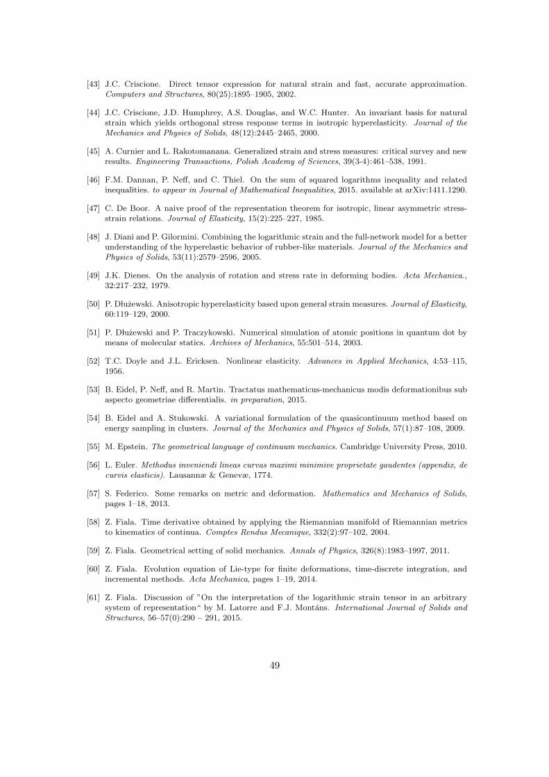
[43] J.C. Criscione. Direct tensor expression for natural strain and fast, accurate approximation.Computers and Structures, 80(25):1895–1905, 2002.

[44] J.C. Criscione, J.D. Humphrey, A.S. Douglas, and W.C. Hunter. An invariant basis for naturalstrain which yields orthogonal stress response terms in isotropic hyperelasticity. Journal of theMechanics and Physics of Solids, 48(12):2445–2465, 2000.

[45] A. Curnier and L. Rakotomanana. Generalized strain and stress measures: critical survey and newresults. Engineering Transactions, Polish Academy of Sciences, 39(3-4):461–538, 1991.

[46] F.M. Dannan, P. Neff, and C. Thiel. On the sum of squared logarithms inequality and relatedinequalities. to appear in Journal of Mathematical Inequalities, 2015. available at arXiv:1411.1290.

[47] C. De Boor. A naive proof of the representation theorem for isotropic, linear asymmetric stress-strain relations. Journal of Elasticity, 15(2):225–227, 1985.

[48] J. Diani and P. Gilormini. Combining the logarithmic strain and the full-network model for a betterunderstanding of the hyperelastic behavior of rubber-like materials. Journal of the Mechanics andPhysics of Solids, 53(11):2579–2596, 2005.

[49] J.K. Dienes. On the analysis of rotation and stress rate in deforming bodies. Acta Mechanica.,32:217–232, 1979.

[50] P. D luzewski. Anisotropic hyperelasticity based upon general strain measures. Journal of Elasticity,60:119–129, 2000.

[51] P. D luzewski and P. Traczykowski. Numerical simulation of atomic positions in quantum dot bymeans of molecular statics. Archives of Mechanics, 55:501–514, 2003.

[52] T.C. Doyle and J.L. Ericksen. Nonlinear elasticity. Advances in Applied Mechanics, 4:53–115,1956.

[53] B. Eidel, P. Neff, and R. Martin. Tractatus mathematicus-mechanicus modis deformationibus subaspecto geometriae differentialis. in preparation, 2015.

[54] B. Eidel and A. Stukowski. A variational formulation of the quasicontinuum method based onenergy sampling in clusters. Journal of the Mechanics and Physics of Solids, 57(1):87–108, 2009.

[55] M. Epstein. The geometrical language of continuum mechanics. Cambridge University Press, 2010.

[56] L. Euler. Methodus inveniendi lineas curvas maximi minimive proprietate gaudentes (appendix, decurvis elasticis). Lausannæ & Genevæ, 1774.

[57] S. Federico. Some remarks on metric and deformation. Mathematics and Mechanics of Solids,pages 1–18, 2013.

[58] Z. Fiala. Time derivative obtained by applying the Riemannian manifold of Riemannian metricsto kinematics of continua. Comptes Rendus Mecanique, 332(2):97–102, 2004.

[59] Z. Fiala. Geometrical setting of solid mechanics. Annals of Physics, 326(8):1983–1997, 2011.

[60] Z. Fiala. Evolution equation of Lie-type for finite deformations, time-discrete integration, andincremental methods. Acta Mechanica, pages 1–19, 2014.

[61] Z. Fiala. Discussion of ”On the interpretation of the logarithmic strain tensor in an arbitrarysystem of representation“ by M. Latorre and F.J. Montans. International Journal of Solids andStructures, 56–57(0):290 – 291, 2015.

49

[62] J. Finger. Das Potential der inneren Krafte und die Beziehungen zwischen den Deformationen undden Spannungen in elastisch isotropen Korpern bei Berucksichtigung von Gliedern, die bezuglichder Deformationselemente von dritter, beziehungsweise zweiter Ordnung sind. Sitzungsberichte derAkademie der Wissenschaften in Wien, 44, 1894.

[63] A. Fischle and P. Neff. The quadratic Cosserat shear-stretch energy (Part I): a general parameterreduction formula and energy-minimizing microrotations in 2D. in preparation, 2015.

[64] A. Fischle, P. Neff, and O. Sander. Numerical comparison of nonlinear hyperelastic formulations,including the Hencky energy and the exponentiated Hencky energy. in preparation, 2015.

[65] J.E. Fitzgerald. A tensorial Hencky measure of strain and strain rate for finite deformations.Journal of Applied Physics, 51(10):5111–5115, 1980.

[66] P.J. Flory. Thermodynamic relations for high elastic materials. Transactions of the FaradaySociety, 57:829–838, 1961.

[67] R.L. Fosdick and A.S. Wineman. On general measures of deformation. Acta Mechanica, 6(4):275–295, 1968.

[68] A.D. Freed. Natural strain. Journal of Engineering Materials and Technology, 117(4):379–385,1995.

[69] A.D. Freed. Hencky strain and logarithmic rates in Lagrangian analysis. International Journal ofEngineering Science, 81:135–145, 2014.

[70] A.D. Freed. Soft Solids. Springer, 2014.

[71] G. Friesecke, R.D. James, and S. Muller. A theorem on geometric rigidity and the derivation ofnonlinear plate theory from three-dimensional elasticity. Communications on Pure and AppliedMathematics, 55(11):1461–1506, 2002.

[72] H. Gercek. Poisson’s ratio values for rocks. International Journal of Rock Mechanics and MiningSciences, 44(1):1–13, 2007.

[73] I.D. Ghiba, P. Neff, and M. Silhavy. The exponentiated Hencky-logarithmic strain energy. Im-provement of planar polyconvexity. International Journal of Non-Linear Mechanics, 71:48–51,2015.

[74] G. Green. On the propagation of light in crystallized media. Transactions of the CambridgePhilosophical Society, 7:121, 1841.

[75] G. Grioli. Una proprieta di minimo nella cinematica delle deformazioni finite. Bollettinodell’Unione Matematica Italiana, 2:252–255, 1940.

[76] G. Grioli. Mathematical Theory of Elastic Equilibrium (recent results), volume 7 of Ergebnisse derangewandten Mathematik. Springer, 1962.

[77] G. Grioli. On the thermodynamic potential for continuums with reversible transformations - somepossible types. Meccanica, 1(1-2):15–20, 1966.

[78] P. Grohs, H. Hardering, and O. Sander. Optimal a priori discretization error bounds for geodesicfinite elements. Foundations of Computational Mathematics, pages 1–55, 2013.

[79] M.E. Gurtin and K. Spear. On the relationship between the logarithmic strain rate and thestretching tensor. International Journal of Solids and Structures, 19(5):437–444, 1983.

50

[80] K. Hackl, A. Mielke, and D. Mittenhuber. Dissipation distances in multiplicative elastoplasticity.In W.L. Wendland and M. Efendiev, editors, Analysis and Simulation of Multifield Problems, pages87–100. Springer, 2003.

[81] M. Hanin and M. Reiner. On isotropic tensor-functions and the measure of deformation. Zeitschriftfur angewandte Mathematik und Physik, 7(5):377–393, 1956.

[82] E. Hartig. Der Elastizitatsmodul des geraden Stabes als Funktion der spezifischen Beanspruchung.Der Civilingenieur, 39:113–138, 1893. available at www.uni-due.de/imperia/md/content/

mathematik/ag_neff/hartig_elastizitaetsmodul.pdf.

[83] P. Haupt. Continuum Mechanics and Theory of Materials. Springer, Heidelberg, 2000.

[84] P. Haupt and C. Tsakmakis. On the application of dual variables in continuum mechanics. Con-tinuum Mechanics and Thermodynamics, 1:165–196, 1989.

[85] D.L. Henann and L. Anand. Fracture of metallic glasses at notches: effects of notch-root radiusand the ratio of the elastic shear modulus to the bulk modulus on toughness. Acta Materialia,57(20):6057–6074, 2009.

[86] D.L. Henann and L. Anand. A large deformation theory for rate-dependent elastic–plastic materialswith combined isotropic and kinematic hardening. International Journal of Plasticity, 25(10):1833–1878, 2009.

[87] D.L. Henann and L. Anand. A large strain isotropic elasticity model based on molecular dynamicssimulations of a metallic glass. Journal of Elasticity, 104(1-2):281–302, 2011.

[88] G.R. Hencky. Obituary of Gerhard R. Hencky, son of Heinrich Hencky, Feb. 9 2014. Publishedin San Francisco Chronicle. available at http://www.legacy.com/obituaries/sfgate/obituary.aspx?pid=169558738.

[89] H. Hencky. Uber den Spannungszustand in kreisrunden Platten mit verschwindenderBiegungssteifigkeit. Zeitschrift fur Mathematik und Physik, 63:311–317, 1915.

[90] H. Hencky. Uber die Beziehungen der Philosophie des ,,Als Ob” zur mathematischenNaturbeschreibung. Annalen der Philosophie, 3:236–245, 1923. available at https://www.uni-due.de/imperia/md/content/mathematik/ag_neff/hencky_als_ob.pdf.

[91] H. Hencky. Uber einige statisch bestimmte Falle des Gleichgewichts in plastischen Korpern.Zeitschrift fur Angewandte Mathematik und Mechanik, 3(4):241–251, 1923.

[92] H. Hencky. Uber die Form des Elastizitatsgesetzes bei ideal elastischen Stoffen. Zeitschrift fur tech-nische Physik, 9:215–220, 1928. available at www.uni-due.de/imperia/md/content/mathematik/

ag_neff/hencky1928.pdf.

[93] H. Hencky. Das Superpositionsgesetz eines endlich deformierten relaxationsfahigenelastischen Kontinuums und seine Bedeutung fur eine exakte Ableitung der Gleichungenfur die zahe Flussigkeit in der Eulerschen Form. Annalen der Physik, 394(6):617–630,1929. available at https://www.uni-due.de/imperia/md/content/mathematik/ag_neff/hencky_superposition1929.pdf.

[94] H. Hencky. Welche Umstande bedingen die Verfestigung bei der bildsamen Verformung von festenisotropen Korpern? Zeitschrift fur Physik, 55:145–155, 1929. available at www.uni-due.de/

imperia/md/content/mathematik/ag_neff/hencky1929.pdf.

[95] H. Hencky. The law of elasticity for isotropic and quasi-isotropic substances by finite deforma-tions. Journal of Rheology, 2(2):169–176, 1931. available at https://www.uni-due.de/imperia/

md/content/mathematik/ag_neff/henckyjrheology31.pdf.

51

www.uni-due.de/imperia/md/content/mathematik/ag_neff/hartig_elastizitaetsmodul.pdf

www.uni-due.de/imperia/md/content/mathematik/ag_neff/hartig_elastizitaetsmodul.pdf

http://www.legacy.com/obituaries/sfgate/obituary.aspx?pid=169558738

http://www.legacy.com/obituaries/sfgate/obituary.aspx?pid=169558738

https://www.uni-due.de/imperia/md/content/mathematik/ag_neff/hencky_als_ob.pdf

https://www.uni-due.de/imperia/md/content/mathematik/ag_neff/hencky_als_ob.pdf

www.uni-due.de/imperia/md/content/mathematik/ag_neff/hencky1928.pdf


https://www.uni-due.de/imperia/md/content/mathematik/ag_neff/hencky_superposition1929.pdf

https://www.uni-due.de/imperia/md/content/mathematik/ag_neff/hencky_superposition1929.pdf



https://www.uni-due.de/imperia/md/content/mathematik/ag_neff/henckyjrheology31.pdf

https://www.uni-due.de/imperia/md/content/mathematik/ag_neff/henckyjrheology31.pdf

[96] H. Hencky. The elastic behavior of vulcanized rubber. Rubber Chemistry and Technology, 6(2):217–224, 1933. available at https://www.uni-due.de/imperia/md/content/mathematik/ag_neff/

hencky_vulcanized_rubber.pdf.

[97] N.J. Higham. Matrix nearness problems and applications. University of Manchester. Departmentof Mathematics, 1988.

[98] N.J. Higham. Functions of Matrices: Theory and Computation. Society for Industrial and AppliedMathematics, Philadelphia, PA, USA, 2008.

[99] R. Hill. On constitutive inequalities for simple materials - I. Journal of the Mechanics and Physicsof Solids, 11:229–242, 1968.

[100] R. Hill. Constitutive inequalities for isotropic elastic solids under finite strain. Proceedings of theRoyal Society of London. A. Mathematical and Physical Sciences, 314:457–472, 1970.

[101] R. Hill. Aspects of invariance in solid mechanics. Advances in Applied Mechanics, 18:1–75, 1978.

[102] A. Hoger. The stress conjugate to logarithmic strain. International Journal of Solids and Struc-tures, 23:1645–1656, 1987.

[103] R. Hooke. Lectures de potentia restitutiva, or of Spring, Explaining the Power of Springy Bodies(1678). In R.T. Gunther, editor, Early Science in Oxford, Volume VIII: The Cutler Lectures ofRobert Hooke. Oxford University Press, 1931.

[104] H. Hopf and W. Rinow. Uber den Begriff der vollstandigen differentialgeometrischen Flache.Commentarii Mathematici Helvetici, 3(1):209–225, 1931.

[105] J.W. Hutchinson and K.W. Neale. Finite strain J2 deformation theory. In Proceedings of theIUTAM Symposium on Finite Elasticity, pages 237–247. Springer, 1982.

[106] A. Imbert. Recherches theoriques et experimentales sur l’elasticite du caoutchouc. Goyard, Lyon,1880. available at www.uni-due.de/imperia/md/content/mathematik/ag_neff/imbert_rubber.

pdf.

[107] D.F. Jones and L.R.G. Treloar. The properties of rubber in pure homogeneous strain. Journal ofPhysics D: Applied Physics, 8(11):1285, 1975.

[108] J. Jost. Riemannian Geometry and Geometric Analysis (2nd ed.). Springer, 1998.

[109] G.R. Kirchhoff. Uber die Gleichungen des Gleichgewichtes eines elastischen Korpers beinicht unendlich kleinen Verschiebungen seiner Theile. Sitzungsberichte der Mathematisch-Naturwissenschaftlichen Classe der Kaiserlichen Akademie der Wissenschaften in Wien, IX, 1852.

[110] J. Lankeit, P. Neff, and Y. Nakatsukasa. The minimization of matrix logarithms: On a fundamentalproperty of the unitary polar factor. Linear Algebra and its Applications, 449(0):28–42, 2014.

[111] M. Latorre and F.J. Montans. On the interpretation of the logarithmic strain tensor in an arbitrarysystem of representation. International Journal of Solids and Structures, 51(7):1507–1515, 2014.

[112] H. Le Dret and A. Raoult. The quasiconvex envelope of the Saint Venant–Kirchhoff stored energyfunction. Proceedings of the Royal Society of Edinburgh: Section A Mathematics, 125(06):1179–1192, 1995.

[113] T. Lehmann. Anisotrope plastische Formanderungen. Romanian Journal of Technical Sciences.Applied Mechanics, 17:1077–1086, 1972.

52

https://www.uni-due.de/imperia/md/content/mathematik/ag_neff/hencky_vulcanized_rubber.pdf

https://www.uni-due.de/imperia/md/content/mathematik/ag_neff/hencky_vulcanized_rubber.pdf

www.uni-due.de/imperia/md/content/mathematik/ag_neff/imbert_rubber.pdf

www.uni-due.de/imperia/md/content/mathematik/ag_neff/imbert_rubber.pdf

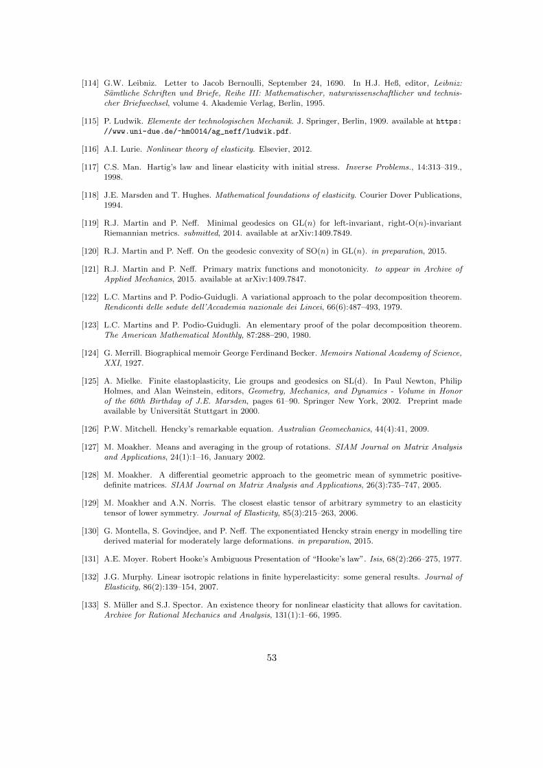
[114] G.W. Leibniz. Letter to Jacob Bernoulli, September 24, 1690. In H.J. Heß, editor, Leibniz:Samtliche Schriften und Briefe, Reihe III: Mathematischer, naturwissenschaftlicher und technis-cher Briefwechsel, volume 4. Akademie Verlag, Berlin, 1995.

[115] P. Ludwik. Elemente der technologischen Mechanik. J. Springer, Berlin, 1909. available at https://www.uni-due.de/~hm0014/ag_neff/ludwik.pdf.

[116] A.I. Lurie. Nonlinear theory of elasticity. Elsevier, 2012.

[117] C.S. Man. Hartig’s law and linear elasticity with initial stress. Inverse Problems., 14:313–319.,1998.

[118] J.E. Marsden and T. Hughes. Mathematical foundations of elasticity. Courier Dover Publications,1994.

[119] R.J. Martin and P. Neff. Minimal geodesics on GL(n) for left-invariant, right-O(n)-invariantRiemannian metrics. submitted, 2014. available at arXiv:1409.7849.

[120] R.J. Martin and P. Neff. On the geodesic convexity of SO(n) in GL(n). in preparation, 2015.

[121] R.J. Martin and P. Neff. Primary matrix functions and monotonicity. to appear in Archive ofApplied Mechanics, 2015. available at arXiv:1409.7847.

[122] L.C. Martins and P. Podio-Guidugli. A variational approach to the polar decomposition theorem.Rendiconti delle sedute dell’Accademia nazionale dei Lincei, 66(6):487–493, 1979.

[123] L.C. Martins and P. Podio-Guidugli. An elementary proof of the polar decomposition theorem.The American Mathematical Monthly, 87:288–290, 1980.

[124] G. Merrill. Biographical memoir George Ferdinand Becker. Memoirs National Academy of Science,XXI, 1927.

[125] A. Mielke. Finite elastoplasticity, Lie groups and geodesics on SL(d). In Paul Newton, PhilipHolmes, and Alan Weinstein, editors, Geometry, Mechanics, and Dynamics - Volume in Honorof the 60th Birthday of J.E. Marsden, pages 61–90. Springer New York, 2002. Preprint madeavailable by Universitat Stuttgart in 2000.

[126] P.W. Mitchell. Hencky’s remarkable equation. Australian Geomechanics, 44(4):41, 2009.

[127] M. Moakher. Means and averaging in the group of rotations. SIAM Journal on Matrix Analysisand Applications, 24(1):1–16, January 2002.

[128] M. Moakher. A differential geometric approach to the geometric mean of symmetric positive-definite matrices. SIAM Journal on Matrix Analysis and Applications, 26(3):735–747, 2005.

[129] M. Moakher and A.N. Norris. The closest elastic tensor of arbitrary symmetry to an elasticitytensor of lower symmetry. Journal of Elasticity, 85(3):215–263, 2006.

[130] G. Montella, S. Govindjee, and P. Neff. The exponentiated Hencky strain energy in modelling tirederived material for moderately large deformations. in preparation, 2015.

[131] A.E. Moyer. Robert Hooke’s Ambiguous Presentation of “Hooke’s law”. Isis, 68(2):266–275, 1977.

[132] J.G. Murphy. Linear isotropic relations in finite hyperelasticity: some general results. Journal ofElasticity, 86(2):139–154, 2007.

[133] S. Muller and S.J. Spector. An existence theory for nonlinear elasticity that allows for cavitation.Archive for Rational Mechanics and Analysis, 131(1):1–66, 1995.

53

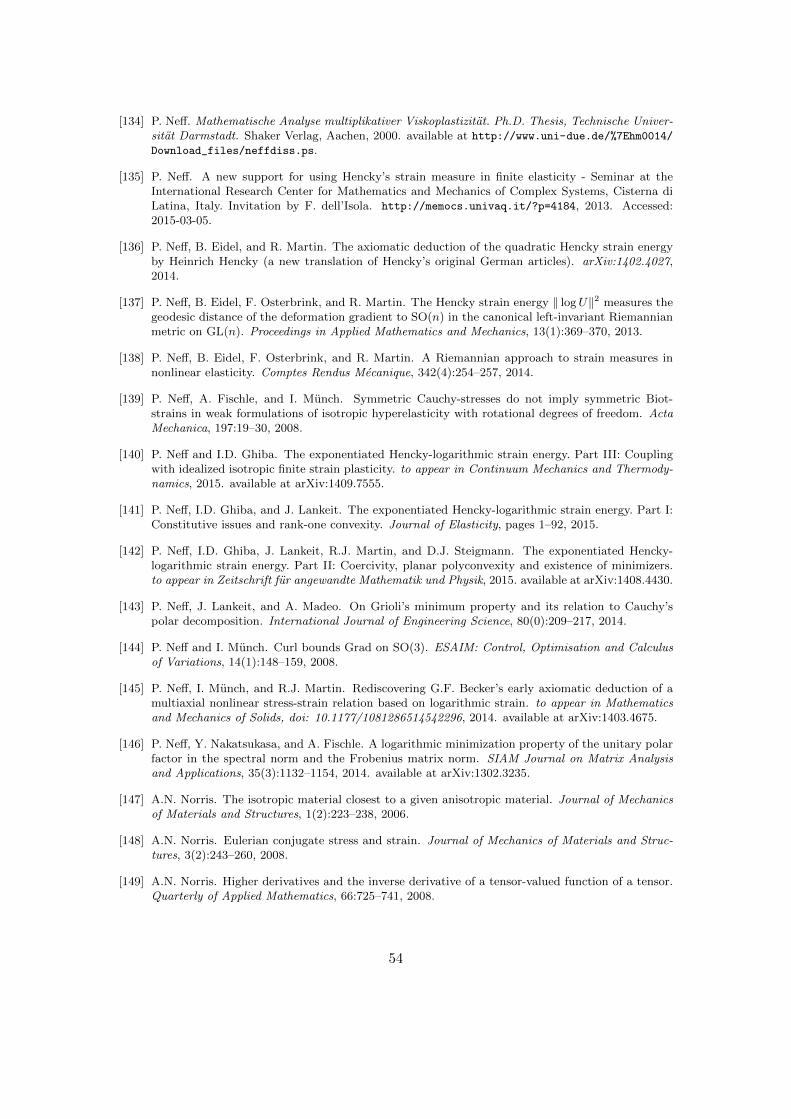
https://www.uni-due.de/~hm0014/ag_neff/ludwik.pdf

https://www.uni-due.de/~hm0014/ag_neff/ludwik.pdf

[134] P. Neff. Mathematische Analyse multiplikativer Viskoplastizitat. Ph.D. Thesis, Technische Univer-sitat Darmstadt. Shaker Verlag, Aachen, 2000. available at http://www.uni-due.de/%7Ehm0014/

Download_files/neffdiss.ps.

[135] P. Neff. A new support for using Hencky’s strain measure in finite elasticity - Seminar at theInternational Research Center for Mathematics and Mechanics of Complex Systems, Cisterna diLatina, Italy. Invitation by F. dell’Isola. http://memocs.univaq.it/?p=4184, 2013. Accessed:2015-03-05.

[136] P. Neff, B. Eidel, and R. Martin. The axiomatic deduction of the quadratic Hencky strain energyby Heinrich Hencky (a new translation of Hencky’s original German articles). arXiv:1402.4027,2014.

[137] P. Neff, B. Eidel, F. Osterbrink, and R. Martin. The Hencky strain energy ‖ logU‖2 measures thegeodesic distance of the deformation gradient to SO(n) in the canonical left-invariant Riemannianmetric on GL(n). Proceedings in Applied Mathematics and Mechanics, 13(1):369–370, 2013.

[138] P. Neff, B. Eidel, F. Osterbrink, and R. Martin. A Riemannian approach to strain measures innonlinear elasticity. Comptes Rendus Mecanique, 342(4):254–257, 2014.

[139] P. Neff, A. Fischle, and I. Munch. Symmetric Cauchy-stresses do not imply symmetric Biot-strains in weak formulations of isotropic hyperelasticity with rotational degrees of freedom. ActaMechanica, 197:19–30, 2008.

[140] P. Neff and I.D. Ghiba. The exponentiated Hencky-logarithmic strain energy. Part III: Couplingwith idealized isotropic finite strain plasticity. to appear in Continuum Mechanics and Thermody-namics, 2015. available at arXiv:1409.7555.

[141] P. Neff, I.D. Ghiba, and J. Lankeit. The exponentiated Hencky-logarithmic strain energy. Part I:Constitutive issues and rank-one convexity. Journal of Elasticity, pages 1–92, 2015.

[142] P. Neff, I.D. Ghiba, J. Lankeit, R.J. Martin, and D.J. Steigmann. The exponentiated Hencky-logarithmic strain energy. Part II: Coercivity, planar polyconvexity and existence of minimizers.to appear in Zeitschrift fur angewandte Mathematik und Physik, 2015. available at arXiv:1408.4430.

[143] P. Neff, J. Lankeit, and A. Madeo. On Grioli’s minimum property and its relation to Cauchy’spolar decomposition. International Journal of Engineering Science, 80(0):209–217, 2014.

[144] P. Neff and I. Munch. Curl bounds Grad on SO(3). ESAIM: Control, Optimisation and Calculusof Variations, 14(1):148–159, 2008.

[145] P. Neff, I. Munch, and R.J. Martin. Rediscovering G.F. Becker’s early axiomatic deduction of amultiaxial nonlinear stress-strain relation based on logarithmic strain. to appear in Mathematicsand Mechanics of Solids, doi: 10.1177/1081286514542296, 2014. available at arXiv:1403.4675.

[146] P. Neff, Y. Nakatsukasa, and A. Fischle. A logarithmic minimization property of the unitary polarfactor in the spectral norm and the Frobenius matrix norm. SIAM Journal on Matrix Analysisand Applications, 35(3):1132–1154, 2014. available at arXiv:1302.3235.

[147] A.N. Norris. The isotropic material closest to a given anisotropic material. Journal of Mechanicsof Materials and Structures, 1(2):223–238, 2006.

[148] A.N. Norris. Eulerian conjugate stress and strain. Journal of Mechanics of Materials and Struc-tures, 3(2):243–260, 2008.

[149] A.N. Norris. Higher derivatives and the inverse derivative of a tensor-valued function of a tensor.Quarterly of Applied Mathematics, 66:725–741, 2008.

54

http://www.uni-due.de/%7Ehm0014/Download_files/neffdiss.ps

http://www.uni-due.de/%7Ehm0014/Download_files/neffdiss.ps

http://memocs.univaq.it/?p=4184

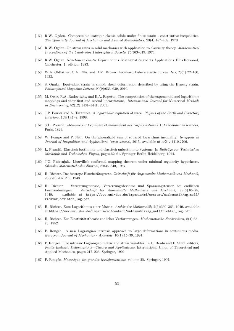
[150] R.W. Ogden. Compressible isotropic elastic solids under finite strain - constitutive inequalities.The Quarterly Journal of Mechanics and Applied Mathematics, 23(4):457–468, 1970.

[151] R.W. Ogden. On stress rates in solid mechanics with application to elasticity theory. MathematicalProceedings of the Cambridge Philosophical Society, 75:303–319, 1974.

[152] R.W. Ogden. Non-Linear Elastic Deformations. Mathematics and its Applications. Ellis Horwood,Chichester, 1. edition, 1983.

[153] W.A. Oldfather, C.A. Ellis, and D.M. Brown. Leonhard Euler’s elastic curves. Isis, 20(1):72–160,1933.

[154] S. Onaka. Equivalent strain in simple shear deformation described by using the Hencky strain.Philosophical Magazine Letters, 90(9):633–639, 2010.

[155] M. Ortiz, R.A. Radovitzky, and E.A. Repetto. The computation of the exponential and logarithmicmappings and their first and second linearizations. International Journal for Numerical Methodsin Engineering, 52(12):1431–1441, 2001.

[156] J.P. Poirier and A. Tarantola. A logarithmic equation of state. Physics of the Earth and PlanetaryInteriors, 109(1):1–8, 1998.

[157] S.D. Poisson. Memoire sur l’equilibre et mouvement des corps elastiques. L’Academie des sciences,Paris, 1829.

[158] W. Pompe and P. Neff. On the generalized sum of squared logarithms inequality. to appear inJournal of Inequalities and Applications (open access), 2015. available at arXiv:1410.2706.

[159] L. Prandtl. Elastisch bestimmte und elastisch unbestimmte Systeme. In Beitrage zur TechnischenMechanik und Technischen Physik, pages 52–61. Springer Berlin Heidelberg, 1924.

[160] J.G. Resetnjak. Liouville’s conformal mapping theorem under minimal regularity hypotheses.Sibirskii Matematicheskii Zhurnal, 8:835–840, 1967.

[161] H. Richter. Das isotrope Elastizitatsgesetz. Zeitschrift fur Angewandte Mathematik und Mechanik,28(7/8):205–209, 1948.

[162] H. Richter. Verzerrungstensor, Verzerrungsdeviator und Spannungstensor bei endlichenFormanderungen. Zeitschrift fur Angewandte Mathematik und Mechanik, 29(3):65–75,1949. available at https://www.uni-due.de/imperia/md/content/mathematik/ag_neff/

richter_deviator_log.pdf.

[163] H. Richter. Zum Logarithmus einer Matrix. Archiv der Mathematik, 2(5):360–363, 1949. availableat https://www.uni-due.de/imperia/md/content/mathematik/ag_neff/richter_log.pdf.

[164] H. Richter. Zur Elastizitatstheorie endlicher Verformungen. Mathematische Nachrichten, 8(1):65–73, 1952.

[165] P. Rougee. A new Lagrangian intrinsic approach to large deformations in continuous media.European Journal of Mechanics - A/Solids, 10(1):15–39, 1991.

[166] P. Rougee. The intrinsic Lagrangian metric and stress variables. In D. Besdo and E. Stein, editors,Finite Inelastic Deformations—Theory and Applications, International Union of Theoretical andApplied Mechanics, pages 217–226. Springer, 1992.

[167] P. Rougee. Mecanique des grandes transformations, volume 25. Springer, 1997.

55

https://www.uni-due.de/imperia/md/content/mathematik/ag_neff/richter_deviator_log.pdf

https://www.uni-due.de/imperia/md/content/mathematik/ag_neff/richter_deviator_log.pdf

https://www.uni-due.de/imperia/md/content/mathematik/ag_neff/richter_log.pdf

[168] P. Rougee. An intrinsic Lagrangian statement of constitutive laws in large strain. Computers andStructures, 84(17):1125–1133, 2006.

[169] O. Sander. Geodesic finite elements of higher order. to appear in IMA Journal of NumericalAnalysis, 2015. preprint available at http://www.igpm.rwth-aachen.de/Download/reports/pdf/IGPM356_k.pdf.

[170] C. Sansour. On the dual variable of the logarithmic strain tensor, the dual variable of the Cauchystress tensor, and related issues. International Journal of Solids and Structures, 38:9221–9232,2001.

[171] J. Schroder, P. Neff, and D. Balzani. A variational approach for materially stable anisotropichyperelasticity. International Journal of Solids and Structures, 42(15):4352–4371, 2005.

[172] J. Schroder, P. Neff, and V. Ebbing. Anisotropic polyconvex energies on the basis of crystallo-graphic motivated structural tensors. Journal of the Mechanics and Physics of Solids, 56(12):3486–3506, 2008.

[173] T. Sendova and J.R. Walton. On strong ellipticity for isotropic hyperelastic materials based uponlogarithmic strain. International Journal of Non-Linear Mechanics, 40(2):195–212, 2005.

[174] B.R. Seth. Generalized strain measure with applications to physical problems. Technical report,Defense Technical Information Center, 1961.

[175] R.T. Shield. Inverse deformation results in finite elasticity. Zeitschrift fur angewandte Mathematikund Physik, 18(4):490–500, 1967.

[176] S. Shrivastava, C. Ghosh, and J.J. Jonas. A comparison of the von Mises and Hencky equivalentstrains for use in simple shear experiments. Philosophical Magazine, 92(7):779–786, 2012.

[177] F. Sidoroff. Sur les restrictions a imposer a l’energie de deformation d’un materiau hyperelastique.Comptes Rendus de l’Academie des Sciences, 279:379–382, 1974.

[178] M. Silhavy. The mechanics and thermomechanics of continuous media. Texts and Monographs inPhysics. Springer, 1997.

[179] M. Silhavy. Rank 1 convex hulls of isotropic functions in dimension 2 by 2. Mathematica Bohemica,126(2):521–529, 2001.

[180] E.B. Tadmor and R.E. Miller. Modeling materials: continuum, atomistic and multiscale techniques.Cambridge University Press, 2011.

[181] R.I. Tanner and E. Tanner. Heinrich Hencky: a rheological pioneer. Rheologica Acta, 42(1-2):93–101, 2003.

[182] A. Tarantola. Elements for Physics: Quantities, Qualities, and Intrinsic Theories. Springer,Heidelberg, 2006.

[183] A. Tarantola. Stress and strain in symmetric and asymmetric elasticity. available atarXiv:0907.1833, 2009.

[184] C. Truesdell. Mechanical foundations of elasticity and fluid dynamics. Journal of Rational Me-chanics and Analysis, 1:125–300, 1952.

[185] C. Truesdell. Hypo-elasticity. Journal of Rational Mechanics and Analysis, 4(1):83–131, 1955.

[186] C. Truesdell. The simplest rate theory of pure elasticity. Communications on Pure and AppliedMathematics, 8(1):123–132, 1955.

56

http://www.igpm.rwth-aachen.de/Download/reports/pdf/IGPM356_k.pdf

http://www.igpm.rwth-aachen.de/Download/reports/pdf/IGPM356_k.pdf

[187] C. Truesdell. Das ungeloste Hauptproblem der endlichen Elastizitatstheorie. Zeitschrift fur Ange-wandte Mathematik und Mechanik, 36(3-4):97–103, 1956.

[188] C. Truesdell and W. Noll. The non-linear field theories of mechanics. In S. Flugge, editor, Handbuchder Physik, volume III/3. Springer, Heidelberg, 1965.

[189] C. Truesdell and R. Toupin. The classical field theories. In S. Flugge, editor, Handbuch der Physik,volume III/1. Springer, Heidelberg, 1960.

[190] C. Vallee. Lois de comportement elastique isotropes en grandes deformations. International Journalof Engineering Science, 16(7):451–457, 1978.

[191] C. Vallee, D. Fortune, and C. Lerintiu. On the dual variable of the Cauchy stress tensor in isotropicfinite hyperelasticity. Comptes Rendus Mecanique, 336(11):851–855, 2008.

[192] B. Vandereycken, P.-A. Absil, and S. Vandewalle. A Riemannian geometry with complete geodesicsfor the set of positive semidefinite matrices of fixed rank. IMA Journal of Numerical Analysis,33:481–514, 2013.

[193] J.P. Wilber and J.C. Criscione. The Baker-Ericksen inequalities for hyperelastic models using anovel set of invariants of Hencky strain. International Journal of Solids and Structures, 42(5):1547–1559, 2005.

[194] H. Xiao. Hencky strain and Hencky model: extending history and ongoing tradition. MultidisciplineModeling in Materials and Structures, 1(1):1–52, 2005.

[195] H. Xiao, O.T. Bruhns, and A. Meyers. Logarithmic strain, logarithmic spin and logarithmic rate.Acta Mechanica, 124(1–4):89–105, 1997.

[196] H. Xiao, O.T. Bruhns, and A. Meyers. Existence and uniqueness of the integrable-exactly hy-

poelastic equationτ = λ(trD)I + 2µD and its significance to finite inelasticity. Acta Mechanica,

138(1):31–50, 1999.

[197] E. Zacur, M. Bossa, and S. Olmos. Multivariate tensor-based morphometry with a right-invariantRiemannian distance on GL+(n). Journal of Mathematical Imaging and Vision, 50:19–31, 2014.

[198] P.A. Zhilin, H. Altenbach, E.A. Ivanova, and A. Krivtsov. Material strain tensor. In GeneralizedContinua as Models for Materials, pages 321–331. Springer, 2013.

57

A. Appendix

A.1. Notation

• R is the set of real numbers,

• R+ = (0,∞) is the set of positive real numbers,

• Rn is the set of real column vectors of length n,

• Rn×n is the set of real n× n-matrices,

• 1 is the identity tensor ;

• XT is the transpose of a matrix X ∈ Rn×m,

• tr(X) =∑n

i=1Xi,i is the trace of X ∈ Rn×n,

• Cof X is the cofactor of X ∈ Rn×n,

• 〈X,Y 〉 = tr(XTY ) =∑n

i,j=1Xi,jYi,j is the canonical inner product on Rn×n,

• ‖X‖ =√〈X,X〉 is the Frobenius matrix norm on Rn×n,

• symX = 12(X +XT ) is the symmetric part of X ∈ Rn×n,

• skewX = 12(X −XT ) is the skew-symmetric part of X ∈ Rn×n,

• devnX = X − 1n tr(X) · 1 is the n-dimensional deviator of X ∈ Rn×n,

• 〈X,Y 〉µ,µc,κ = µ 〈devn symX,devn symY 〉+µc 〈skewX, skew Y 〉+ κ2 tr(X) tr(Y ) is the

weighted inner product on Rn×n,

• ‖X‖µ,µc,κ =√〈X,X〉µ,µc,κ is the weighted Frobenius norm on Rn×n,

• GL(n) = A ∈ Rn×n | detA 6= 0 is the general linear group of all invertible A ∈ Rn×n,

• GL+(n) = A ∈ Rn×n | detA > 0 is the identity component of GL(n),

• SL(n) = A ∈ Rn×n | detA = 1 is the special linear group of all A ∈ GL(n) withdetA = 1,

• O(n) is the orthogonal group of all Q ∈ Rn×n with QTQ = 1,

• SO(n) is the special orthogonal group of all Q ∈ O(n) with detQ = 1,

• Sym(n) is the set of symmetric, real n× n-matrices, i.e. ST = S for all S ∈ Sym(n),

• PSym(n) is the set of positive definite, symmetric, real n× n-matrices, i.e. xTPx > 0for all P ∈ PSym(n), 0 6= x ∈ Rn,

58

• gl(n) = Rn×n is the Lie algebra of all real n× n-matrices,

• so(n) = W ∈ Rn×n |W T = −W is the Lie algebra of skew symmetric, real n × n-matrices,

• sl(n) = X ∈ Rn×n | tr(X) = 0 is the Lie algebra of trace free, real n × n-matrices,i.e. tr(X) = 0 for all X ∈ sl(n),

• Ω ⊂ Rn is the reference configuration of an elastic body,

• ∇f = Df is the first derivative of a differentiable function f

• curl v denotes the curl of a vector valued function v : R3 → R3,

• Curl p denotes the curl of a matrix valued function p : R3 → R3×3, taken row-wise,

• ϕ : Ω→ Rn is a continuously differentiable deformation with ∇ϕ(x) ∈ GL+(n) for allx ∈ Ω,

• F = ∇ϕ ∈ GL+(n) is the deformation gradient,

• U =√F TF ∈ PSym(n) is the right Biot-stretch tensor,

• V =√FF T ∈ PSym(n) is the left Biot-stretch tensor,

• B = FF T = V 2 is the Finger tensor,

• C = F TF = U2 is the right Cauchy-Green deformation tensor,

• F = RU = V R is the polar decomposition of F with R = polar(F ) ∈ SO(n),

• E0 = logU is the material Hencky strain tensor,

• E0 = log V is the spatial Hencky strain tensor,

• S1 = DFW (F ) is the first Piola-Kirchhoff stress corresponding to an elastic energyW = W (F ),

• S2 = F−1 S1 = 2DCW (C) is the second Piola-Kirchhoff stress corresponding to anelastic energy W = W (C) (Doyle-Ericksen formula),

• τ = S1 FT = Dlog VW (log V ) [116, p. 116] is the Kirchhoff stress tensor,

• σ = 1detF τ is the Cauchy stress tensor,

• TBiot = U S2 = DUW (U) is the Biot stress tensor corresponding to an elastic energyW = W (U),

• L = FF−1 is the spatial velocity gradient,

• D = symL is the rate of stretching or spatial strain rate tensor,

• W = skewL is the spatial continuum spin.

59

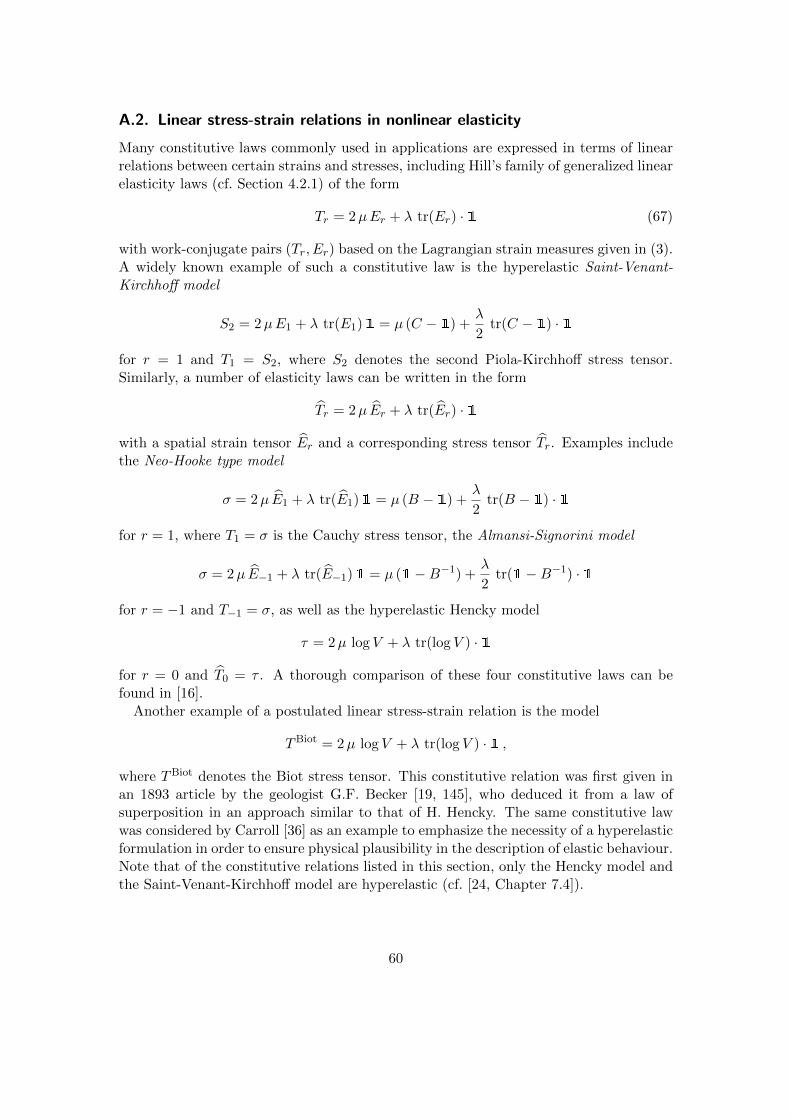
A.2. Linear stress-strain relations in nonlinear elasticity

Many constitutive laws commonly used in applications are expressed in terms of linearrelations between certain strains and stresses, including Hill’s family of generalized linearelasticity laws (cf. Section 4.2.1) of the form

Tr = 2µEr + λ tr(Er) · 1 (67)

with work-conjugate pairs (Tr, Er) based on the Lagrangian strain measures given in (3).A widely known example of such a constitutive law is the hyperelastic Saint-Venant-Kirchhoff model

S2 = 2µE1 + λ tr(E1)1 = µ (C − 1) +λ

2tr(C − 1) · 1

for r = 1 and T1 = S2, where S2 denotes the second Piola-Kirchhoff stress tensor.Similarly, a number of elasticity laws can be written in the form

Tr = 2µ Er + λ tr(Er) · 1

with a spatial strain tensor Er and a corresponding stress tensor Tr. Examples includethe Neo-Hooke type model

σ = 2µ E1 + λ tr(E1)1 = µ (B − 1) +λ

2tr(B − 1) · 1

for r = 1, where T1 = σ is the Cauchy stress tensor, the Almansi-Signorini model

σ = 2µ E−1 + λ tr(E−1)1 = µ (1−B−1) +λ

2tr(1−B−1) · 1

for r = −1 and T−1 = σ, as well as the hyperelastic Hencky model

τ = 2µ log V + λ tr(log V ) · 1

for r = 0 and T0 = τ . A thorough comparison of these four constitutive laws can befound in [16].

Another example of a postulated linear stress-strain relation is the model

TBiot = 2µ log V + λ tr(log V ) · 1 ,

where TBiot denotes the Biot stress tensor. This constitutive relation was first given inan 1893 article by the geologist G.F. Becker [19, 145], who deduced it from a law ofsuperposition in an approach similar to that of H. Hencky. The same constitutive lawwas considered by Carroll [36] as an example to emphasize the necessity of a hyperelasticformulation in order to ensure physical plausibility in the description of elastic behaviour.Note that of the constitutive relations listed in this section, only the Hencky model andthe Saint-Venant-Kirchhoff model are hyperelastic (cf. [24, Chapter 7.4]).

60

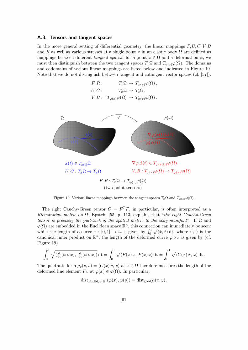
A.3. Tensors and tangent spaces

In the more general setting of differential geometry, the linear mappings F,U,C, V,Band R as well as various stresses at a single point x in an elastic body Ω are defined asmappings between different tangent spaces: for a point x ∈ Ω and a deformation ϕ, wemust then distinguish between the two tangent spaces TxΩ and Tϕ(x)ϕ(Ω). The domainsand codomains of various linear mappings are listed below and indicated in Figure 19.Note that we do not distinguish between tangent and cotangent vector spaces (cf. [57]).

F,R : TxΩ → Tϕ(x)ϕ(Ω) ,

U, C : TxΩ → TxΩ ,

V,B : Tϕ(x)ϕ(Ω) → Tϕ(x)ϕ(Ω) .

ϕ(x(t))

∇ϕ(x(t)).x(t)

x(t)

x(t)

Ω ϕ(Ω)ϕ

x(t) ∈ Tx(t)Ω

U,C : TxΩ → TxΩ

∇ϕ.x(t) ∈ Tϕ(x(t))ϕ(Ω)

V,B : Tϕ(x)ϕ(Ω) → Tϕ(x)ϕ(Ω)

F,R : TxΩ → Tϕ(x)ϕ(Ω)

(two-point tensors)

Figure 19: Various linear mappings between the tangent spaces TxΩ and Tϕ(x)ϕ(Ω).

The right Cauchy-Green tensor C = F TF , in particular, is often interpreted as aRiemannian metric on Ω; Epstein [55, p. 113] explains that “the right Cauchy-Greentensor is precisely the pull-back of the spatial metric to the body manifold”. If Ω andϕ(Ω) are embedded in the Euclidean space Rn, this connection can immediately be seen:while the length of a curve x : [0, 1] → Ω is given by

∫ 10

√〈x, x〉 dt, where 〈·, ·〉 is the

canonical inner product on Rn, the length of the deformed curve ϕ x is given by (cf.Figure 19)∫ 1

0

√〈 d

dt(ϕ x), ddt(ϕ x)〉 dt =

∫ 1

0

√〈F (x) x, F (x) x〉 dt =

∫ 1

0

√〈C(x) x, x〉dt .

The quadratic form gx(v, v) = 〈C(x) v, v〉 at x ∈ Ω therefore measures the length of thedeformed line element Fv at ϕ(x) ∈ ϕ(Ω). In particular,

distEuclid,ϕ(Ω)(ϕ(x), ϕ(y)) = distgeod,Ω(x, y) ,

61

where distEuclid,ϕ(Ω)(ϕ(x), ϕ(y)) = ‖ϕ(x) − ϕ(y)‖ is the Euclidean distance betweenϕ(x), ϕ(y) ∈ ϕ(Ω) and distgeod,Ω(x, y) denotes the geodesic distance between x, y ∈ Ωwith respect to the Riemannian metric gx(v, w) = 〈C(x) v, w〉.

Moreover, this interpretation characterizes the Green-Lagrangian strain tensor E1 =12(C − 1) as a measure of change in length: the difference between the squared lengthof a line element v ∈ TxΩ in the reference configuration and the squared length of thedeformed line element F (x) v ∈ Tϕ(x)Ω is given by

‖F (x) v‖2 − ‖v‖2 = 〈C(x) v, v〉 − 〈v, v〉 = 〈(C(x)− 1) v, v〉 = 2 〈E1(x) v, v〉 ,

where ‖ . ‖ denotes the Euclidean norm on Rn. Note that for F (x) = 1 + ∇u(x) withthe displacement gradient ∇u(x), the expression ‖F (x) v‖2 can be linearized to

‖F (x) v‖2 = ‖(1+∇u(x)) v‖2 = 〈(1+∇u(x)) v, (1+∇u(x)) v〉= 〈v, v〉+ 2 〈∇u(x) v, v〉+ 〈∇u(x) v, ∇u(x) v〉= ‖v‖2 + 2 〈sym∇u(x) v, v〉+ ‖∇u(x) v‖2

= ‖v‖2 + 2 〈sym∇u(x) v, v〉+ h.o.t. ,

where h.o.t. denotes higher order terms with respect to ∇u(x). Thus

‖F (x) v‖2 − ‖v‖2 = 2 〈ε(x) v, v〉+ h.o.t. ,

where ε = sym∇u is the linear strain tensor.

A.4. Additional computations

Let Cof F = (detF ) · F−T denote the cofactor of F ∈ GL+(n). Then the geodesicdistance of Cof F to SO(n) with respect to the Riemannian metric g introduced in (18)can be computed directly by applying Theorem 3.3:

dist2geod(Cof F,SO(n))

= µ ‖devn log√

(Cof F )T Cof F‖2 +κ

2

[tr(

log√

(Cof F )T Cof F)]2

= µ ‖ devn log√

(detF )2 · F−1F−T ‖2 +κ

2

[tr(

log√

(detF )2 · F−1F−T)]2

= µ ‖ devn log√F−1F−T ‖2 +

κ

2

[tr(

log((detF ) · 1

)+ log

√F−1F−T

)]2

= µ ‖ devn log(U−1)‖2 +κ

2[tr((ln detF ) · 1+ log(U−1)

)]2

= µ ‖ − devn logU‖2 +κ

2[n · (ln detU)− tr(logU)]2

= µ ‖ devn logU‖2 +κ (n− 1)2

2[tr(logU)]2 .

62

A.5. The principal matrix logarithm on PSym(n) and the matrixexponential

The following lemma states some basic computational rules for the matrix exponentialexp : Rn×n → GL+(n) and the principal matrix logarithm log : PSym(n) → Sym(n)

involving the trace operator tr and the deviatoric part devnX = X − tr(X)n · 1 of a

matrix X ∈ Rn×n.

Lemma A.1. Let X ∈ Rn×n, P ∈ PSym(n) and c > 0. Then

i) det(exp(X)) = etr(X) ,

ii) exp(devnX) = e−tr(X)n · exp(X) ,

iii) log(c · 1) = ln(c) · log(1) ,

iv) log((detP )−1/n · P ) = logP − ln(detP )n · 1 = devn logP .

Proof. Equality i) is well known (see e.g. [23]). Equality iii) follows directly from thefact that exp : Sym(n)→ PSym(n) is bijective and that exp(ln(c) ·1) = eln(c) ·1 = c ·1.Since AB = BA implies exp(AB) = exp(A) exp(B), we find

exp(devnX) = exp(X − tr(X)

n· 1) = exp(X) · exp(−tr(X)

n· 1) = exp(X) · e−

tr(X)n · 1 ,

showing ii). For iv), note that

tr(logP ) = ln(detP ) =⇒ logP − ln(detP )n · 1 = devn logP ,

and

exp(devn logP ) = e−tr(logP )

n · exp(logP )

=(eln(detP )

)−1/n· P = (detP )−1/n · P .

according to ii). Then the injectivity of the matrix exponential on Sym(n) shows iv).

63

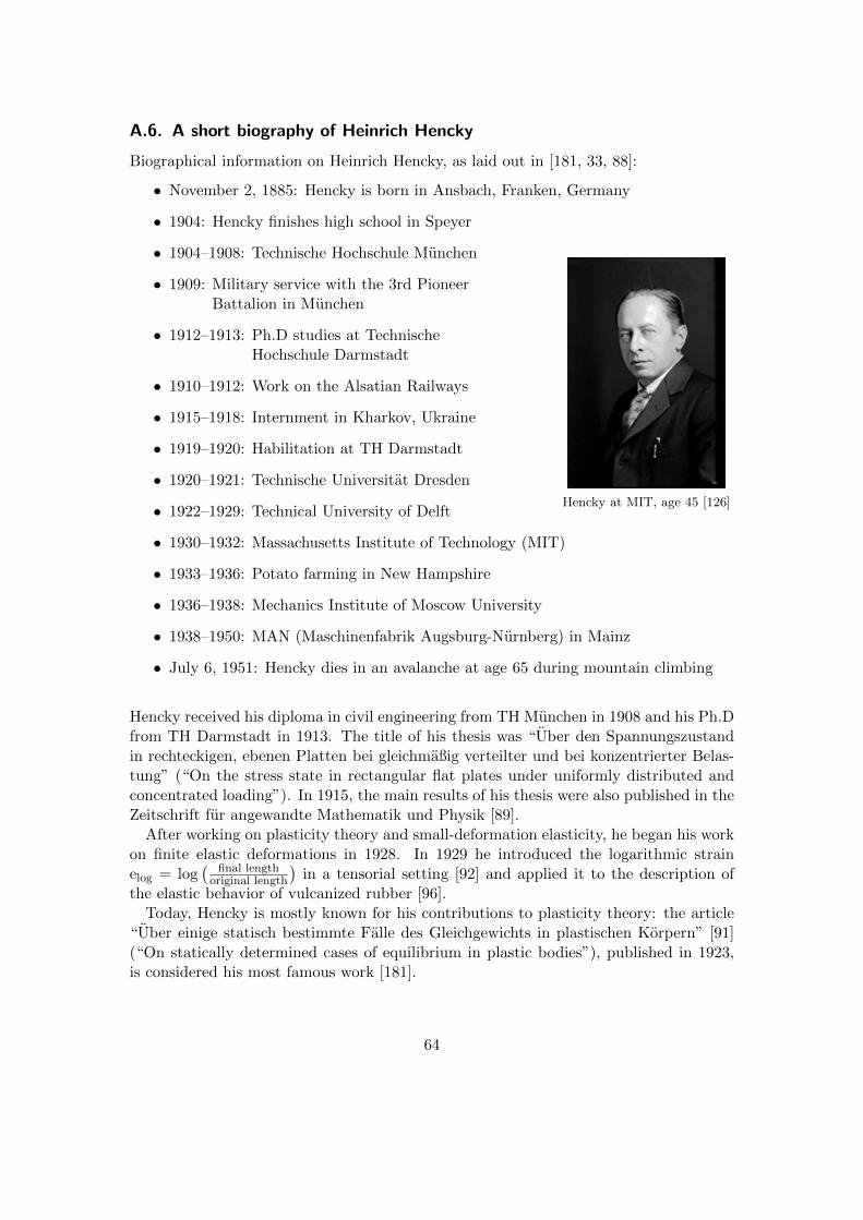
A.6. A short biography of Heinrich Hencky

Hencky at MIT, age 45 [126]

Biographical information on Heinrich Hencky, as laid out in [181, 33, 88]:

• November 2, 1885: Hencky is born in Ansbach, Franken, Germany

• 1904: Hencky finishes high school in Speyer

• 1904–1908: Technische Hochschule Munchen

• 1909: Military service with the 3rd PioneerBattalion in Munchen

• 1912–1913: Ph.D studies at TechnischeHochschule Darmstadt

• 1910–1912: Work on the Alsatian Railways

• 1915–1918: Internment in Kharkov, Ukraine

• 1919–1920: Habilitation at TH Darmstadt

• 1920–1921: Technische Universitat Dresden

• 1922–1929: Technical University of Delft

• 1930–1932: Massachusetts Institute of Technology (MIT)

• 1933–1936: Potato farming in New Hampshire

• 1936–1938: Mechanics Institute of Moscow University

• 1938–1950: MAN (Maschinenfabrik Augsburg-Nurnberg) in Mainz

• July 6, 1951: Hencky dies in an avalanche at age 65 during mountain climbing

Hencky received his diploma in civil engineering from TH Munchen in 1908 and his Ph.Dfrom TH Darmstadt in 1913. The title of his thesis was “Uber den Spannungszustandin rechteckigen, ebenen Platten bei gleichmaßig verteilter und bei konzentrierter Belas-tung” (“On the stress state in rectangular flat plates under uniformly distributed andconcentrated loading”). In 1915, the main results of his thesis were also published in theZeitschrift fur angewandte Mathematik und Physik [89].

After working on plasticity theory and small-deformation elasticity, he began his workon finite elastic deformations in 1928. In 1929 he introduced the logarithmic strainelog = log

( final lengthoriginal length

)in a tensorial setting [92] and applied it to the description of

the elastic behavior of vulcanized rubber [96].Today, Hencky is mostly known for his contributions to plasticity theory: the article

“Uber einige statisch bestimmte Falle des Gleichgewichts in plastischen Korpern” [91](“On statically determined cases of equilibrium in plastic bodies”), published in 1923,is considered his most famous work [181].

64

Geometry of logarithmic strain measures in solid mechanicshm0014/ag_neff/publikation_neu/Geometry...

Documents

Transcript of Geometry of logarithmic strain measures in solid mechanicshm0014/ag_neff/publikation_neu/Geometry...