DISSERTATION

Geometry, Constraints and Computation of theTrifocal Tensor

ausgeführt zum Zwecke der Erlangung des akademischen Grades eines Doktors dertechnischen Wissenschaften unter Leitung von

Prof. Dr.-Ing. Wolfgang FörstnerInstitut für Photogrammetrie, Universität Bonn

in Zusammenarbeit mit

O.Univ.Prof. Dipl.-Ing. Dr.techn. Karl KrausInstitut für Photogrammetrie und Fernerkundung (E122),

Technische Universität Wien

eingereicht an der Technische Universität WienFakultät für Naturwissenschaften und Informatik

von

Dipl.-Ing. Camillo ResslMatr.Nr 8926567

Flurschützstrasse 1/21A-1120 Wien

Wien, im Juni 2003 . . . . . . . . . . . . . . . . . .

Diese Arbeit ist Teil des Forschungsprojekts „Bildorientierung in verschiedenen Disziplinen“und wurde vom Fonds zur Förderung der wissenschaftlichen Forschung (FWF) unter Projekt-Nr. P13901-INF unterstützt.

This work is part of the research project “Image orientation in different disciplines” and wassupported by the Austrian Science Fund under project no. P13901-INF.

ii

Abstract

The topic of this thesis is the trifocal tensor, which describes the relative orientation (or epipo-lar geometry) of three uncalibrated images. So it plays the same role for three images as thefundamental matrix plays for two. The trifocal tensor is a homogenous valence-(1,2) tensor,which means that it can be represented as a 3×3×3 cube of numbers. It is of particular interestbecause of the following properties:

– The trifocal tensor can be determined linearly from corresponding points and lines in threeimages; the latter are not useable for the fundamental matrix. Consequently the trifocal ten-sor provides a tool to determine the relative orientation of three images without requiring approxi-mate values. This orientation can be used to initialize a subsequent bundle block adjustment.Furthermore, the chances of running into critical configurations for determining the trifocaltensor is much smaller than for two images and the fundamental matrix. The only practicallyrelevant critical configuration for computing the trifocal tensor happens if all correspondingimage features arise from a common plane in space.

After determining the trifocal tensor, the basis vectors and rotation matrices of the relativeorientation of the three images can be extracted easily if the interior orientation of the imagesis known. If the interior orientation is unknown, but the same for all three images, then, ingeneral, this common interior orientation can be retrieved also.

If n > 3 images are given, then many unrelated trifocal tensors are computed. Before all n im-ages can be used simultaneously, the individual basis vectors and rotation matrices derivedfrom the unrelated tensors must be transformed into one common system.

– The transfer relations associated with the trifocal tensor can be used to transfer the content(points and lines) of two source images into the other one (the target image). If the targetimage is a real image, the transferred position of features can be used to initialize a matchingtechnique in the target image. If the target image is virtual with a given orientation, then thetransfer relations can be used to form the content of this new image by transferring pixel bypixel. This process is called novel view synthesis or image formation.

In this thesis we concentrate on the first issue of determining the trifocal tensor.

Each triple of points provides 4 equations, called trilinearities, which are linear in the tensorelements and each corresponding triple of lines provides 2 linear equations. Since the tensoris made up of 27 elements, at least 7 points, 13 lines or a proper combination are needed for adirect linear solution of the trifocal tensor.

There are, however, some drawbacks associated with this linear solution. The trifocal tensoris made up of 27 elements, but it only has 18 degrees of freedom. Consequently its elementshave to satisfy 8 internal constraints, besides the fixing of the scale ambiguity, to represent avalid trifocal tensor. These constraints are in generally not satisfied by the direct linear solution.Another drawback is that the direct linear solution does not minimize the errors in the originalpoint and line measurements (so-called reprojection error) but some other quantities (so-calledalgebraic error).

These drawbacks can be prevented by determining a valid trifocal tensor by minimizing re-projection error. The so-called Gauss-Helmert model provides a general environment for suchconstrained adjustment tasks. The determination of a valid trifocal tensor in the Gauß-Helmert

iii

model can be done basically in two ways: By parameterizing the tensor using its 27 elementsand introducing the 8 internal constraints together with the scale fixing, or by using an alterna-tive parameterization for the trifocal tensor that has 18 degrees of freedom.

Several sets of constraints and alternative parameterizations have been proposed over the yearsand the most important ones are reviewed in this thesis. Most of these constraints and param-eterizations are derived from the so-called tensorial slices, which are 3×3 matrices that can besliced out of the tensor. Due to their great importance these tensorial slices are investigatedthoroughly in this thesis. Using these tensorial slices we derive two new sets of constraintstogether with a simple geometric interpretation, and also a new alternative parameterizationfor the trifocal tensor.

For computing a valid trifocal tensor by minimizing reprojection error in the Gauß-Helmertmodel it is important to have a consistent representation for the trifocal tensor. The param-eterization using the projection matrices proposed by Hartley is the simplest way for such aconsistent representation. This parameterization is applicable as long as (i) not all three projec-tion centers coincide and (ii) the first projection center is different from the other two.

If all image features arise from a common plane in space, the trifocal tensor can not be com-puted uniquely. Therefore the minimum thickness of the object points used to compute the trifo-cal tensor is investigated; i.e. what is the minimum deviation of the object points from a com-mon plane, so that the computation is still possible? This investigation will be done empiricallyfor different image configurations and different numbers of corresponding points. In these in-vestigations we further consider the effect on the computed tensor if the internal constraintsare considered or neglected, and if algebraic error or reprojection error is minimized.

The findings of these empirical investigations can be summarized in the following way: Forimage configurations with strong geometry, like in the case of convergent terrestrial images orin the case of aerial images, the direct linear solution (algebraic error without constraints) forthe trifocal tensor and the valid tensor from the Gauß-Helmert model (reprojection error withconstraints) are practically the same. Concerning the minimum thickness unexpected smallvalues were found already for 10 point correspondences. If the number of points increases, theminimum thickness gets even smaller. For the mentioned configurations and 15 point corre-spondences the computation of the trifocal tensor is still successful for a minimum thickness ofthe object points of about 1% of the camera distance (normal angle camera with assumed noisein the images of 1 pixel).

For image configurations with weak geometry, like collinear projection centers with congruentviewing directions, much more point correspondences are required and the direct linear solu-tion fails more often for small thicknesses of the object points than the valid solution from theGauß-Helmert model.

From these empirical investigations we come to the conclusion that minimizing reprojection er-ror and considering the internal constraints is actually not necessary if the image configurationhas a strong geometry – especially if one is only interested in initial values for a subsequentbundle block adjustment. However, if a general tool for providing such initial values is aimedfor, which does not have any restrictions on the image geometry and also handles weak con-figurations, then the Gauß-Helmert model minimizing reprojection error must be applied.

iv

Kurzfassung

Das Thema dieser Arbeit ist der Trifokal-Tensor, der die relative Orientierung (oder Epipo-largeometrie) von drei unkalibrierten Bildern beschreibt. In diesem Sinne ist der Tensor eine Er-weiterung der Fundamental-Matrix, welche die relative Orientierung von zwei unkalibriertenBildern beschreibt. Der Trifokal-Tensor ist ein homogener Tensor der Stufe 3; dem gemäß kanner als 3×3×3 Zahlenwürfel dargestellt werden. Aufgrund der folgenden Eigenschaften ist die-ser Tensor von besonderem Interesse:

– Der Trifokal-Tensor kann in linearer Weise aus gegebenen Punkt- und Linienkorresponden-zen in drei Bildern bestimmt werden; letztere sind für die Bestimmung der Fundamental-Matrix nicht verwendbar. Aus diesem Grund stellt der Trifokal-Tensor ein Werkzeug für dieBestimmung der relativen Orientierung von drei Bildern dar, für das keine Näherungswerte benö-tigt werden. Diese so gefundene Orientierung kann dann als Startwert für eine anschließen-de Bündelblockausgleichung verwendet werden. Weiters ist die Wahrscheinlichkeit auf einegefährliche Konfiguration zu treffen, die keine eindeutige Bestimmung des Tensors erlaubt,wesentlich geringer als für zwei Bilder und ihre Fundamental-Matrix. Die einzige praktischrelevante gefährliche Situation entsteht nur dann, wenn alle korrespondierenden Bildpunkteund -linien von einer gemeinsamen Ebene stammen.

Nachdem der Trifokal-Tensor bestimmt wurde, können die Basisvektoren und Rotationsma-trizen der relativen Orientierung der drei Bilder einfach extrahiert werden – wenn die innereOrientierung bekannt ist. Ist diese unbekannt, aber ident für alle drei Bilder, so kann diesegemeinsame innere Orientierung ebenfalls im Allgemeinen bestimmt werden.

Sind n > 3 Bilder gegeben, so werden mehrere unzusammenhängende Trifokal-Tensorenberechnet. Bevor alle n Bilder gemeinsam weiterverarbeitet werden können, müssen die ein-zelnen unzusammenhängenden Basisvektoren und Rotationsmatrizen in ein gemeinsamesSystem transformiert werden.

– Die sogenannten Transferbeziehungen, die sich aus dem Trifokal-Tensor ableiten lassen, kön-nen verwendet werden, um den Inhalt (Punkte und Geraden) von zwei Quellbildern in einanderes Bild – das Zielbild – zu transferieren. Falls dieses Zielbild eine echtes Bild ist, dannkönnen die transferierten Positionen verwendet werden um ein Matching-Verfahren zu star-ten. Falls dieses Zielbild eine virtuelles Bild mit gegebener Orientierung darstellt, dann kannder Inhalt dieses neuen Bildes mit Hilfe der Transferrelationen Pixel für Pixel aus den beidenQuellbildern aufgebaut werden. Dieser Vorgang wird im Englischen als novel view synthesisoder image formation bezeichnet.

In dieser Arbeit wird der erste Punkt – die Berechnung des Trifokal-Tensors – näher behandelt.

Jedes Triple von korrespondierenden Punkten liefert 4 Gleichungen, die sogenannten Trilinea-ritäten, welche linear in den 27 Tensorelementen sind. Jedes Tripel von korrespondierendenGeraden liefert 2 lineare Gleichungen. Demzufolge benötigt man mindestens 7 Punkte, 13 Ge-raden oder eine passende Kombination um den Trifokal-Tensor direkt bestimmen zu können.

Mit dieser direkten linearen Lösung für den Trifokal-Tensor sind allerdings ein paar Nachteileverbunden. Der Trifokal-Tensor besteht zwar aus 27 Elementen, jedoch besitzt er nur 18 Frei-heitsgrade. Aus diesem Grund müssen die Tensorelemente 8 interne Bedingungen erfüllen, ne-ben der Festlegung des Tensormaßstabes, um einen gültigen Trifokal-Tensor zu repräsentieren.

v

Diese Bedingungen werden im Allgemeinen von der direkten linearen Lösung nicht erfüllt. Einweiterer Nachteil ist, dass die direkte lineare Lösung nicht die Fehler in den originalen Bild-beobachtungen minimiert (die sogenannten Residuen), sondern den sogenannten algebraischenFehler.

Diese Nachteile kann man beseitigen, wenn man einen gültigen Trifokal-Tensor über die Mi-nimierung der Bildresiduen berechnet. Das sogenannte Gauß-Helmert Modell stellt eine all-gemeine Umgebung für derartige bedingte Ausgleichungsaufgaben dar. Die Berechnung einesgültigen Trifokal-Tensor im Gauß-Helmert Modell kann in zwei Arten realisiert werden: Indemder Trifokal-Tensor durch seine 27 Elemente repräsentiert wird und die 8 internen Bedingungengemeinsam mit der Festlegung des Maßstabes zusätzlich ins Gauß-Helmert Modell aufgenom-men werden; oder indem der Trifokal-Tensor durch eine andere alternative Parametrisierung,die genau 18 Freiheitsgrade hat, dargestellt wird.

Verschiedene Gruppen von Bedingungen und unterschiedliche Parametrisierungen wurdenin der Vergangenheit publiziert, und die wichtigsten davon werden in dieser Arbeit zusam-mengefasst. Die meisten dieser Bedingungen und Parametrisierungen leiten sich aus den so-genannten Tensorschnitten ab. Dabei handelt es sich um 3×3 Matrizen, die aus dem Tensorsozusagen herausgeschnitten werden können. Aufgrund ihrer hohen Bedeutung werden dieseTensorschnitte in dieser Arbeit sehr genau untersucht. Mit ihrer Hilfe werden zwei neue Grup-pen von Bedingungen, die auch eine einfache geometrische Interpretation erlauben, und eineneue alternative Parametrisierung für den Trifokal-Tensor hergeleitet.

Um nun einen gültigen Trifokal-Tensor im Gauß-Helmert Modell über die Minimierung derBildresiduen berechnen zu können, ist es wichtig eine konsistente Repräsentierung für denTensor zu besitzen. Die von Hartley vorgeschlagene Parametrisierung mit Hilfe der Projekti-onsmatrizen ist die einfachste Möglichkeit für solch eine konsistente Repräsentierung. DieseParametrisierung ist anwendbar solange (i) nicht alle drei Projektionszentren zusammenfallenund (ii) das erste Projektionszentrum verschieden von den anderen beiden ist.

Wenn alle Korrespondenzen in den drei Bildern von einer gemeinsamen Ebene stammen, dannkann der Trifokal-Tensor nicht eindeutig bestimmt werden. Aus diesem Grund wird in dieserArbeit die minimaler Dicke der Objektpunkte untersucht; d.h. was ist die minimal notwendi-ge Abweichung von einer gemeinsamen Ebene, sodass der Trifokal-Tensor immer noch er-folgreich berechnet werden kann? Diese Untersuchung wird empirisch anhand verschiedenerBildkonfigurationen und unterschiedlicher Punktanzahl durchgeführt. In diesen Untersuchun-gen werden weiters die Unterschiede im berechneten Trifokal-Tensor behandelt, die entstehenwenn die internen Bedingungen berücksichtigt werden oder nicht, und wenn algebraische Feh-ler oder Bildresiduen minimiert werden.

Die Erkenntnisse dieser empirischen Untersuchungen können wie folgt zusammengefasst wer-den: Für Bildkonfigurationen mit guter Geometrie, wie im Fall von konvergenten terrestrischenAufnahmen oder im Fall von Luftbildern, stimmt die direkte lineare Lösung (algebraischerFehler ohne Bedingungen) für den Tensor praktisch mit dem gültigen Tensor, der im Gauß-Helmert Modell (Bildresiduen mit Bedingungen) geschätzt wird überein. Für diese Konfigura-tionen mit guter Geometrie wurden auch erstaunlich geringe minimale Dicken bereits bei derVerwendung von 10 korrespondierenden Punkten gefunden. Nimmt die Anzahl der Punkte zu,so wird auch die minimale Dicke kleiner. Für die erwähnten Konfigurationen und 15 Punkttri-pel war die Berechung des Tensors für eine minimale Dicke von etwa 1% der Aufnahmeentfer-nung immer noch erfolgreich (Normalwinkel Aufnahmen und angenommenes Bildrauschenvon 1 Pixel).

vi

Für Bildkonfigurationen mit schwacher Geometrie, wie im Fall von kollinearen Projektions-zentren mit zusammenfallenden Blickrichtungen, ist eine deutlich größere Punkteanzahl istnotwendig und die direkte lineare Lösung versagt viel häufiger bei kleinen Objektdicken alsdie gültige Lösung übers Gauß-Helmert Modell.

Diese empirischen Untersuchungen führen uns zum Schluss, dass für Konfigurationen mit gu-ter Geometrie die Minimierung der Bildresiduen und die Berücksichtigung der internen Bedin-gungen eigentlich nicht notwendig ist – besonders dann nicht, wenn man nur an Näherungs-werten für eine anschließende Bündelblockausgleichung interessiert ist. Benötigt man jedochein allgemeines Werkzeug, das Näherungswerte für die Bildorientierungen liefert und keineEinschränkungen an die Bildkonfiguration setzt und auch bei schwächerer Geometrie funktio-niert, so ist die Lösung übers Gauß-Helmert Modell zu realisieren.

vii

Contents

1 Introduction 1

1.1 Overview . . . . . . . . . . . . . . . . . . . . . . . . . . . . . . . . . . . . . . . . . . 1

1.2 Motivation . . . . . . . . . . . . . . . . . . . . . . . . . . . . . . . . . . . . . . . . . 2

1.2.1 The photogrammetric viewpoint . . . . . . . . . . . . . . . . . . . . . . . . 2

1.2.2 The computer vision viewpoint . . . . . . . . . . . . . . . . . . . . . . . . . 4

1.3 Objective of the thesis . . . . . . . . . . . . . . . . . . . . . . . . . . . . . . . . . . . 6

1.4 Overview of the thesis . . . . . . . . . . . . . . . . . . . . . . . . . . . . . . . . . . 7

2 A few Words about Notation 9

3 Projective Geometry 10

3.1 Introduction . . . . . . . . . . . . . . . . . . . . . . . . . . . . . . . . . . . . . . . . 10

3.2 The projective plane IP2 . . . . . . . . . . . . . . . . . . . . . . . . . . . . . . . . . . 11

3.3 The projective spaces IP3 and IPn . . . . . . . . . . . . . . . . . . . . . . . . . . . . 15

3.3.1 The Plücker line coordinates . . . . . . . . . . . . . . . . . . . . . . . . . . 16

3.4 Projective transformations in IPn . . . . . . . . . . . . . . . . . . . . . . . . . . . . 19

3.5 Constructing new entities in IP2 and IP3 . . . . . . . . . . . . . . . . . . . . . . . . 22

3.5.1 Projective transformations of lines in IP3 . . . . . . . . . . . . . . . . . . . 25

3.5.2 Transformation of S(), I I() and I() for a given point transformation H . . 26

3.6 Checking the identity of points and lines in IP2 . . . . . . . . . . . . . . . . . . . . 27

3.7 Conditioning of projective relations . . . . . . . . . . . . . . . . . . . . . . . . . . 27

4 A few Basics on Tensor Calculus 29

viii

5 Single Image Geometry 32

5.1 The pinhole camera model . . . . . . . . . . . . . . . . . . . . . . . . . . . . . . . . 32

5.2 The mapping of points – the projection matrix P . . . . . . . . . . . . . . . . . . . 34

5.3 The mapping of lines – the projection matrix Q . . . . . . . . . . . . . . . . . . . 37

5.4 The back projection of points and lines . . . . . . . . . . . . . . . . . . . . . . . . . 39

6 Two-View Geometry 40

6.1 The relative orientation of two images . . . . . . . . . . . . . . . . . . . . . . . . . 40

6.1.1 Epipolar geometry . . . . . . . . . . . . . . . . . . . . . . . . . . . . . . . . 42

6.1.2 The fundamental matrix . . . . . . . . . . . . . . . . . . . . . . . . . . . . . 42

6.1.3 The essential matrix . . . . . . . . . . . . . . . . . . . . . . . . . . . . . . . 46

6.1.4 Retrieving the basis vector and the rotation matrix from the essential matrix 47

6.1.5 Historical notes . . . . . . . . . . . . . . . . . . . . . . . . . . . . . . . . . . 49

6.2 Homographies and dual correlations between two images . . . . . . . . . . . . . 49

6.2.1 Homographies between two images induced by a plane . . . . . . . . . . 50

6.2.2 Dual correlations between two images induced by a 3D line . . . . . . . . 54

7 Three-View Geometry – the Trifocal Tensor 58

7.1 A derivation of the trifocal tensor . . . . . . . . . . . . . . . . . . . . . . . . . . . . 58

7.1.1 Computing the trifocal tensor from given projection matrices . . . . . . . 62

7.2 The tensorial slices . . . . . . . . . . . . . . . . . . . . . . . . . . . . . . . . . . . . 63

7.2.1 The correlation slices . . . . . . . . . . . . . . . . . . . . . . . . . . . . . . . 63

7.2.2 The homography slices . . . . . . . . . . . . . . . . . . . . . . . . . . . . . 67

7.2.3 Rank combinations . . . . . . . . . . . . . . . . . . . . . . . . . . . . . . . . 73

7.3 The trilinearities . . . . . . . . . . . . . . . . . . . . . . . . . . . . . . . . . . . . . . 74

7.4 Retrieving the orientation parameters . . . . . . . . . . . . . . . . . . . . . . . . . 80

7.4.1 Retrieving the epipoles . . . . . . . . . . . . . . . . . . . . . . . . . . . . . . 80

7.4.2 Retrieving the fundamental matrices . . . . . . . . . . . . . . . . . . . . . . 83

7.4.3 Retrieving the projection matrices . . . . . . . . . . . . . . . . . . . . . . . 87

7.4.4 Retrieving the common interior orientation of the three images . . . . . . 88

7.4.5 Retrieving the relative orientation of three calibrated images . . . . . . . . 90

7.4.6 Transformation of the individual relative orientations into one commonframe in case of n > 3 images . . . . . . . . . . . . . . . . . . . . . . . . . . 91

ix

7.5 Changing the order of the images . . . . . . . . . . . . . . . . . . . . . . . . . . . . 92

7.6 The internal constraints . . . . . . . . . . . . . . . . . . . . . . . . . . . . . . . . . 93

7.6.1 The non-minimal set of Papadopoulo and Faugeras . . . . . . . . . . . . . 93

7.6.2 The minimal set of Canterakis . . . . . . . . . . . . . . . . . . . . . . . . . 94

7.6.3 The new minimal sets of constraints . . . . . . . . . . . . . . . . . . . . . . 96

7.7 Historical notes . . . . . . . . . . . . . . . . . . . . . . . . . . . . . . . . . . . . . . 104

8 The Computation of the Trifocal Tensor 107

8.1 The direct linear solution . . . . . . . . . . . . . . . . . . . . . . . . . . . . . . . . . 108

8.2 Minimizing reprojection error . . . . . . . . . . . . . . . . . . . . . . . . . . . . . . 109

8.3 The constrained solution . . . . . . . . . . . . . . . . . . . . . . . . . . . . . . . . . 112

8.3.1 The parameterization using the projection matrices . . . . . . . . . . . . . 113

8.3.2 The six-point parameterization . . . . . . . . . . . . . . . . . . . . . . . . . 114

8.3.3 The minimal parameterization by Papadopoulo and Faugeras . . . . . . . 118

8.3.4 A new parameterization . . . . . . . . . . . . . . . . . . . . . . . . . . . . . 119

8.3.5 Considering the internal constraints in the Gauß-Helmert model . . . . . 124

8.4 Transformation of the trifocal tensor due to conditioning . . . . . . . . . . . . . . 127

8.5 Critical configurations for determining the trifocal tensor . . . . . . . . . . . . . . 128

9 Empirical Investigations concerning the Quality of the estimated Trifocal Tensor 130

9.1 The setup . . . . . . . . . . . . . . . . . . . . . . . . . . . . . . . . . . . . . . . . . . 131

9.2 The plots of the ground errors and the percentage of failures with respect to thevariation of the cuboid . . . . . . . . . . . . . . . . . . . . . . . . . . . . . . . . . . 139

9.2.1 Variation of the cuboid and 1 pixel noise in the images . . . . . . . . . . . 139

9.2.2 Variation of the cuboid and 10 pixel noise in the images . . . . . . . . . . . 139

9.3 Investigation of the results . . . . . . . . . . . . . . . . . . . . . . . . . . . . . . . . 139

9.3.1 Configuration ’Tetra’ . . . . . . . . . . . . . . . . . . . . . . . . . . . . . . . 153

9.3.2 Configuration ’Air1’ . . . . . . . . . . . . . . . . . . . . . . . . . . . . . . . 153

9.3.3 Configuration ’Air2’ . . . . . . . . . . . . . . . . . . . . . . . . . . . . . . . 154

9.3.4 Configuration ’Street1’ . . . . . . . . . . . . . . . . . . . . . . . . . . . . . . 155

9.3.5 Configuration ’Street2’ . . . . . . . . . . . . . . . . . . . . . . . . . . . . . . 156

9.4 Summary . . . . . . . . . . . . . . . . . . . . . . . . . . . . . . . . . . . . . . . . . . 158

x

10 Conclusion 162

10.1 Summary . . . . . . . . . . . . . . . . . . . . . . . . . . . . . . . . . . . . . . . . . . 162

10.2 Contribution of this thesis . . . . . . . . . . . . . . . . . . . . . . . . . . . . . . . . 164

10.3 Outlook . . . . . . . . . . . . . . . . . . . . . . . . . . . . . . . . . . . . . . . . . . . 166

A Notation 168

B Matrix Calculus 171

B.1 The eigenvalue problem . . . . . . . . . . . . . . . . . . . . . . . . . . . . . . . . . 171

B.2 The singular value decomposition . . . . . . . . . . . . . . . . . . . . . . . . . . . 172

B.3 The cross product . . . . . . . . . . . . . . . . . . . . . . . . . . . . . . . . . . . . . 173

B.4 The Kronecker product and the vec ()-operator . . . . . . . . . . . . . . . . . . . 174

B.5 Miscellaneous . . . . . . . . . . . . . . . . . . . . . . . . . . . . . . . . . . . . . . . 175

C The Algebraic Derivation of the Multiple View Tensors 176

D Least Squares Adjustment 182

D.1 Introduction . . . . . . . . . . . . . . . . . . . . . . . . . . . . . . . . . . . . . . . . 182

D.2 The Mathematical Model . . . . . . . . . . . . . . . . . . . . . . . . . . . . . . . . . 183

D.2.1 Error properties of observations . . . . . . . . . . . . . . . . . . . . . . . . 183

D.3 Methods for parameter estimation . . . . . . . . . . . . . . . . . . . . . . . . . . . 184

D.3.1 Parameterization . . . . . . . . . . . . . . . . . . . . . . . . . . . . . . . . . 185

D.4 The Gauß-Markoff model . . . . . . . . . . . . . . . . . . . . . . . . . . . . . . . . 187

D.5 The Gauß-Helmert model . . . . . . . . . . . . . . . . . . . . . . . . . . . . . . . . 188

E MATLAB File Listings 191

E.1 Vanishing derivatives for the essential matrix constraint of identical singular val-ues . . . . . . . . . . . . . . . . . . . . . . . . . . . . . . . . . . . . . . . . . . . . . 191

E.2 Independency of the constraints derived from the homography slices . . . . . . . 193

Bibliography 195

xi

Chapter 1

Introduction

1.1 Overview

The topic of this thesis is the trifocal tensor, which describes the epipolar geometry (or relativeorientation) of three uncalibrated images, just like the fundamental matrix does for two. Thetrifocal tensor is of particular interest because of the following properties:

– The trifocal tensor can be determined linearly from corresponding points and lines in threeimages. Compared to the separate linear determination of the respective three fundamentalmatrices from the same data, which however can only use corresponding points, the lineardetermination of the trifocal tensor should be more stable, as it can use also lines, and allimage correspondences are used at once. Furthermore, the chances of running into criticalconfigurations for determining the trifocal tensor is much smaller than for the fundamentalmatrix. The only practical relevant critical configuration for computing the trifocal tensorhappens if all corresponding image features arise from a common plane in space.

After determining the trifocal tensor, the basis vectors and rotation matrices of the relativeorientation of the three images can be extracted easily if the interior orientation of the imagesis known. If the interior orientation is unknown, but the same for all three images, then, ingeneral, this common interior orientation can be retrieved also.

– The transfer relations associated with the trifocal tensor can be used to transfer the content(points and lines) of two source images into the other one (the target image). If the targetimage is a real image, the transferred position of features can be used to initialize a matchingtechnique in the target image. If the target image is virtual with a given orientation, then thetransfer relations can be used to form the content of this new image by transferring pixel bypixel. This process is called novel view synthesis or image formation.

A similar transfer can also be realized with fundamental matrices, but there the transfer oflines as entities is not possible and the transfer of points can fail for certain configurations,like collinear projection centers.

So there are many benefits in considering three images with their trifocal tensor comparedto pairs of images with their fundamental matrices. In this thesis we will concentrate on thefirst issue of determining the trifocal tensor. Although in principle the trifocal tensor can bedetermined linearly, there are some drawbacks associated with this direct linear solution.

1

– A valid trifocal tensor satisfies certain internal constraints. The tensor obtained by the directlinear solution does in general not satisfy these internal constraints and so does not representa valid trifocal tensor. Furthermore, depending on the number of point and line correspon-dences, their distribution in space and the arrangement of the three images, chances are thatthe redundant unconstrained elements of the tensor absorb some of the errors in the im-age measurements and thereby return a severely disturbed tensor and thus a rather wrongrelative orientation of the three images.

– This direct linear solution does not minimize the errors in the original measurements (so-called reprojection error) but some other quantities (so-called algebraic error). And thereforewe suspect that additional errors in the tensor elements are induced.

These drawbacks can be removed by determining a valid trifocal tensor by minimizing repro-jection error. The so-called Gauss-Helmert model provides a general environment for such con-strained adjustment tasks. For realizing the determination of the trifocal tensor in this modelwe have to investigate the internal constraints of the trifocal tensor and find ways of intro-ducing them in this model. This can be done either by considering the necessary number ofconstraints explicitly or by using an alternative parameterization, which returns a valid trifocaltensor in any case.

Some set of constraints and alternative parameterizations have been presented over the years.We will review the most important ones and derive also new sets of constraints and a newparameterization. As it turns out, the simplest way of realizing a valid trifocal tensor in theGauß-Helmert model is the parameterization using the projection matrices proposed in [Hart-ley 1994a], which historically is one of the first parameterizations.

If all image features arise from a common plane in space, the trifocal tensor can not be com-puted uniquely. Therefore it is interesting to investigate the minimum deviation from a com-mon plane required to successfully determine the trifocal tensor. This investigation will bedone empirically for different image configurations and different numbers of correspondingpoints. In these investigations we further consider the effect on the computed tensor if theinternal constraints are considered or neglected, and if algebraic error or reprojection error isminimized.

1.2 Motivation

In this thesis concepts of two vision sciences photogrammetry and computer vision are applied.The approaches taken in these two disciplines are guided by different interests and thereforehave different benefits and drawbacks. Consequently it is useful to outline the viewpoint ofeach science individually.

1.2.1 The photogrammetric viewpoint

The main task of photogrammetry is the reconstruction of spatial objects using a set of images.For the reconstruction the object is abstracted by a set of points and line-elements, out of whichlines and surfaces are formed. The 3D coordinates of these special object points and the line-

2

and surface-belongings (the so-called topology) are to be determined. These coordinates haveto be related to a – in most cases – given global coordinate system.

In a geometric manner an image can be interpreted as the result of a central projection. Inphotogrammetry the conventional mathematical representation of the central projection is thefollowing; see e.g. [Kraus 1997]

x = xp0 − cr11(X − XZ) + r21(Y −YZ) + r31(Z− ZZ)r13(X − XZ) + r23(Y −YZ) + r33(Z− ZZ)

y = yp0 − cr12(X − XZ) + r22(Y −YZ) + r32(Z− ZZ)r13(X − XZ) + r23(Y −YZ) + r33(Z− ZZ)

(1.1)

where X, Y, Z are the Cartesian coordinates of an object point. They may be known (controlpoint) or unknown (tie point). The Cartesian coordinates x, y of the corresponding image pointare observed. The principal distance c together with the coordinates of the principal point xp0 ,yp0 form the interior orientation and are known by calibration in most cases. The coordinatesof the projection center XZ, YZ, ZZ and the elements ri j of a spatial rotation matrix R (from theimage- to the object-coordinate-system), constructed by three rotation parameters, make up thethe exterior orientation and are unknown in most cases. Altogether the representation (1.1) isdone using nine parameters in a non-linear way.

A camera whose way of projecting can be described in the presented way is usually called apinhole camera model; see also section 5.1. Photographs made by real cameras deviate more orless from an exact central projection due to errors of the lenses, film deformations or unflatnessof the CCD-sensor; i.e. the pinhole model is not sufficient to describe the reality. These devia-tions are compensated by additional parameters including among others the radial distortion asthe most important one. They are introduced by additive terms in the equations (1.1).

The basic requirement for doing object reconstruction with a set of images is image orientation;i.e. the estimation of the exterior and maybe the interior orientation of all the images. Forsome of these tasks the reference to a global system of coordinates (absolute orientation) is notnecessary or this is done later: in other words, no or insufficient control features are available.In such cases one works with the so-called relative orientation. This is the alignment of at leasttwo images in such a way that corresponding projection rays intersect in a point in space. Theunderlying (local) coordinate system is fixed for example in the following manner: its origincoincides with the projection center of a suitable image and the orientation of the axes of thecoordinate system of that image fix the orientation of the axes of the object system.

Whether one works with a global coordinate system or with a local one of relative orientation,the equations (1.1) always give the fundamental relation between object point and image point.

Least-squares adjustment The observed image coordinates are subject to accidental errors.For decreasing their disturbing influence on the estimated unknowns the number of observa-tions is much higher than the number of unknowns. This results in an overdetermined system,which is then solved by minimizing or maximizing a certain criterion. Any of the followingcriteria is useful. The unknown parameters are estimated such that: (i) they are unbiased andhave least variance, the so-called best unbiased estimation, (ii) the sum of the squared residuals isminimized, the so-called least-squares-estimation, or (iii) the probability for the given realizationof the observations is maximized, the so-called maximum-likelihood-estimation.

3

The optimization of the chosen criterion is realized in a certain mathematical model, which con-sists of a stochastical model and a functional model. The stochastical model describes the stochasticproperties of the observations; e.g. by their covariances or their probability density functions.The functional model describes the functional relations between the observations and the un-known parameters.

Two kinds of functional models are commonly used in geodesy: the Gauß-Markoff model, inwhich each observation can be expressed in terms of the known and unknown parameters,and the Gauß-Helmert model, in which only functions of the observations can be expressed interms of the parameters; see [Koch 1999] and also section D. If the observations are normallydistributed, then the unknown parameters which are estimated in these two models satisfy allthree criteria stated above.

In general, one works with a least-squares-estimation or least-squares-adjustment. But it is im-portant to point out that such a least-squares-adjustment is a best unbiased estimation onlyif the sum of the squares of the errors of the original observations is minimized (so-called re-projection or residual error ) and not the sum of squares of some other quantities, which arefunctionally dependent on groups of observations (so-called algebraic error).

A least-squares-adjustment based on the Gauß-Markoff model is also termed adjustment byindirect observations, and if it is based on the Gauß-Helmert model, it is called general case of leastsquares adjustment. The latter also allows the inclusion of constraints between the unknownparameters. We see from equation (1.1) that the observed image coordinates can be directlyexpressed functionally in the orientation parameters and the object coordinates. Therefore theleast-squares-adjustment of images based on the pinhole camera model can be done in theGauß-Markoff model, which in this case is also called bundle block adjustment.

In the course of such a bundle block adjustment the most plausible values for the unknowns(object points, the exterior and under certain circumstances also the interior orientation of theimages) and their accuracies resp. co-variances are computed. But for such an adjustment linearequations are needed. Since the equations of the central projection are non-linear, they haveto be linearized and the solution needs to be found iteratively. For this purpose approximatevalues of the exterior (and under certain circumstances also for the interior orientation) of theimages are necessary. But in many cases the determination of these approximate values is quitetedious.

1.2.2 The computer vision viewpoint

In computer vision central perspective images are also worked with and the pinhole cameramodel is used, too. The tasks in computer vision that deal specially with the problem of im-age orientation are again object reconstruction (called structure from motion) and further the in-spection of dynamical processes (called 3d-dynamic-scene-analysis, motion from structure or activevision); e.g. inspections in robotics applications or tracking of moving objects like cars.

Due to the highly non-linear character of equation (1.1) in computer vision the central perspec-tive relation between object and image is not described with the 9 elements of the interior andexterior orientation and relation (1.1), but a linear representation is aimed for. This which is es-pecially necessary for the real time applications in active vision. This linear representation forthe central projection is achieved using projective geometry and is obtained in form of a 3×4 ma-trix P – the so-called point projection matrix; see section 5.2. Projective geometry is very suited

4

for representing the geometry of vision problems, because all basic geometric entities – points,lines and planes – can simply be represented as vectors, the vector translation can be repre-sented as a linear mapping and entities at infinity are naturally incorporated in the framework.So also the mapping of 3D lines to image lines, which is rather hard to represent in the classicalnotation of interior and exterior orientation, can be represented linearly using a 3×6 matrix Q– the so-called line projection matrix, which is closely related to P; see section 5.3.

The benefits of using projective geometry go even further, as it also allows a linear representa-tion for the relative orientation of two, three or four images1 by means of homogenous multipleview tensors. The two bifocal tensors – essential matrix resp. fundamental matrix – represent lin-early the relative orientation of two calibrated resp. uncalibrated images. The trifocal tensor isthe linear formulation of the relative orientation of three uncalibrated images and the quadri-focal tensor the one of four uncalibrated images. Linear in this case means that the relationsrepresenting the relative orientation of two, three and four images (i.e. the condition that theback projection of the corresponding image points and lines intersect in space) are linear inthe respective tensor elements and multi-linear in the coordinates of the corresponding imagefeatures.

This linearity, however, is achieved for the price that these projective representations use moreelements than the corresponding conventional representation with the interior and exteriororientation of the images. The homogenous multiple view tensor for n views is made up of 3n

elements but has only 11n− 15 independent elements (also called degrees of freedom). As a con-sequence 3n − (11n− 15) constraints, which are generally non-linear, must hold between theprojective parameters of the linear formulation to represent a valid relative orientation of two,three or four images; see table 1.1. As long as these tensors are computed from known interiorand exterior orientations of given images, this is not a problem, since then the constraints arefulfilled anyway.

number of images number of constraints

2 2

3 9

4 16

Table 1.1: Number of constraints for the linear formulation of the relative orientation of two, three and fouruncalibrated images. Due to the homogeneity of these multiple view tensors, one of these constraints is the fixingof the scale.

Estimating the multiple view tensors The fulfillment of the constraints constitutes a prob-lem if such a tensor is to be determined for given image correspondences (points and/or lines)which are subject to accidental errors. The great benefit of the linearity, which makes the wholematter independent on approximate values, is only applicable if these constraints are neglectedand algebraic error is minimized. This is the total opposite to an optimal solution, which con-siders the constraints and minimizes reprojection error by using the Gauß-Helmert model. TheGauss-Markoff model is not applicable in this case because the above mentioned relations forthe intersections of the back projections of the corresponding image features are multi-linearfunctions in the image coordinates.

1In section C it is shown, that for more than four images no such linear representation is possible.

5

If the interior orientation of the images is known a-priori (especially for photogrammetric cam-eras), then another drawback may arise when determining these tensors linearly. This knowl-edge can not be used because it imposes additional non-linear constraints among the tensorelements. This has the affect that each image is individually calibrated during the linear com-putation. The quality of such self calibrations depends strongly on the image configuration andthe distribution of the object points and lines. For example the calibration and consequently thelinear determination of the tensors fails if all image correspondences arise from planar objectpoints.

On the other hand if the interior orientation of the images is absolutely unknown (e.g. for ama-teur cameras, or for very old images or parts of images of unknown source) and the distributionof the points and lines permits the calibration, this feature turns into a strong benefit.

Another drawback of these projective representations is that non-linear distortion is naturallynot included in this framework. This follows from the fact, that projective geometry is based onmappings called collineations, which map straight lines to straight lines. In the presence of non-linear distortion, however, the mapped line is no longer straight. Some strategies concerningthe inclusion of non-linear distortion parameters into the projective based framework, whichis not considered in this thesis, can be found in the literature; e.g. [Niini 2000] or [Fitzgibbon2001].

1.3 Objective of the thesis

The optimal solution for the multiple view tensors requires the consideration of the actualdegrees of freedom. In the Gauß-Helmert model this can be established in two ways: (i) con-sidering the necessary number of independent constraints or (ii) using an alternative param-eterization for the multiple view tensors, which has the required degrees of freedom. If thisparameterization is minimal, i.e. the number of parameters is the same as the degrees of free-dom, then no constraints need to be considered during the computation in the Gauß-Helmertmodel.

For the essential and fundamental matrix the constraints were investigated many years ago,e.g. [Rinner 1963], [Huang and Faugeras 1989] or [Hartley 1992], and are summarized in sec-tions 6.1.3 and 6.1.2. Minimal parameterizations are presented in [Luong and Faugeras 1996]and [Hartley and Zisserman 2001]. Also for the quadrifocal tensor constraints and parameteri-zations are reported in the literature; see [Hartley 1998] and [Shashua and Wolf 2000].

The subject of this work are constraints and parameterizations for the trifocal tensor. The ten-sor is made up of 27 elements and has 18 degrees of freedom, thus has to satisfy 9 constraints.Several constraints (e.g. [Stein and Shashua 1998], [Papadopoulo and Faugeras 1998] ,[Canter-akis 2000]) and parameterizations ([Hartley 1994a], [Torr and Zisserman 1997], [Papadopouloand Faugeras 1998]) are reported in the literature so far. In most cases their usage in the Gauß-Helmert model, however, is limited due to one or more of the following reasons: They are

– not complete (< 9), like the set of [Stein and Shashua 1998]. Consequently no valid trifocaltensor will result from the computation.

– not minimal (> 9), like the set of [Papadopoulo and Faugeras 1998]. Therefore a suitableminimal subset of those constraints must be select for the Gauß-Helmert model, and it is notclear on which criteria this selection should be based on.

6

– not valid for all image coordinate systems, like the set of [Papadopoulo and Faugeras 1998].Depending on the image coordinate system it may happen that certain constraints are notapplicable. Although this problem can be solved by adapting the coordinate system, thisrequires additional unnecessary attention during the computation.

– rather complicated to be incorporated in the Gauß-Helmert model, like the set of [Canterakis 2000]and the minimal parameterizations of [Torr and Zisserman 1997] and [Papadopoulo andFaugeras 1998]. For this limitation we have to consider that the constraints or the relationsinvolving the alternative parameterization must be linearized to be included in the Gauß-Helmert model. Therefore and if we want to avoid numerical differentiation, the constraintsand parameterization should not be too complex.

The only parameterization so far that can be realized in the Gauß-Helmert model without diffi-culties is the non-minimal parameterization using the projection matrices proposed in [Hartley1994a].

The objective of this work is to investigate the constraints of the trifocal tensor and to derivea minimal set of constraints, that can be included in the Gauß-Helmert model by explicit dif-ferentiation. Two new minimal sets of constraints presented in section 7.6.3 are quite simplecompared to the only minimal set so far presented in the literature [Canterakis 2000]. Theyare, however, not general applicable for all image coordinate systems – just as the set of [Pa-padopoulo and Faugeras 1998].

We also investigate the ways the trifocal tensor can be parameterized and in section 8.3.4 wederive a new non-minimal parameterization from which a minimal parameterization can beobtained quite easily. Although this minimal parameterization is simpler than the other mini-mal parameterizations of [Torr and Zisserman 1997] and [Papadopoulo and Faugeras 1998], itsimplementation in the Gauß-Helmert model is still more complex than for the parameterizationusing the projection matrices.

If all image features arise from a common plane in space, the trifocal tensor can not be com-puted uniquely. Therefore it is interesting to investigate the minimum deviation from a com-mon plane required to successfully determine the trifocal tensor. This investigation will bedone empirically for different image configurations and different numbers of correspondingpoints. In these investigations we further consider the effect on the computed tensor if theinternal constraints are considered or neglected, and if algebraic error or reprojection error isminimized.

1.4 Overview of the thesis

In the chapters 3 to 6 the basics, required to understand the properties of the trifocal tensor, arepresented in detail.

The basics of projective geometry are presented in chapter 3, followed by a short introductionto tensor notation in chapter 4. Contrary to what we might expect from the name trifocal tensorthe usage of tensorial algebra is rather small throughout this work, therefore this introductionis kept short.

7

The single-view geometry is explained in chapter 5, including the pinhole camera model, thepoint and line projection matrices, and the back projection of points and lines in the image toprojection rays and projection planes in space.

The two-view geometry is depicted in chapter 6, including the explanation of the relative orien-tation of images, the epipolar geometry and the fundamental and essential matrix. This chapteris closed by the description of homographies between two images induced by a 3D plane, andcorrelations between two images induced by a 3D line. These two mappings between twoimages will appear frequently when dealing with the trifocal tensor.

The three-view geometry follows in chapter 7, which is also the main chapter of this thesis.First a derivation of the trifocal tensor is given, followed by an investigation of the tensorproperties. These are derived by considering the homographies and correlations associatedwith the trifocal tensor; section 7.2. The trilinearities and transfer relations, which are the basicrelations involving the trifocal tensor, are described in section 7.3. The internal constraints areexplored in section 7.6 by reviewing existing sets and deriving new sets of constraints.

The computation of a valid trifocal tensor by minimizing reprojection error is the topic of chap-ter 8. After reviewing existing ways of parameterizing a valid trifocal tensor a new parame-terization for the trifocal tensor is presented in section 8.3.4. In section 8.3.5 all possible waysof realizing a valid trifocal tensor in the Gauß-Helmert model are discussed critically, showingthat the simplest way is the parameterization using the projection matrices.

The results of empirical investigations showing the differences in determining the trifocal ten-sor by minimizing algebraic error or reprojection error with or without considering the internalconstraints are presented in chapter 9. Here also the effect of almost planar object points is con-sidered.

A summary and a conclusion given in chapter 10 close this thesis.

8

Chapter 2

A few Words about Notation

In a rigorous way a distinction should be made between a geometric object – like a point, a lineor a plane – and its mathematical representation, which is usually a vector. However, for thesake of simplicity and since all geometric objects, except for points, are of interest only in theirprojective representation, this distinction is not performed within this thesis and all geometricobjects are addressed via their projective representation (a homogenous vector) in bold uprightfont. If the Euclidian representation of a point is considered, then this is indicated in boldslanted font.

Since we will deal with points and lines in 2D and 3D and further planes in 3D it is helpfulto recognize these objects directly by their symbolical representations. Therefore the followingnotation was chosen, for a full summary on the used notation see section A on page 168:

2D objects:points

represented as Euclidian vectors: lower case Roman font – slanted, e.g. e, p, xrepresented as homogenous vectors: lower case Roman font – upright, e.g. e, p, x

linesrepresented as homogenous vectors: lower case Greek font, e.g. α, λ, ρ

3D objects:points

represented as Euclidian vectors: upper case Roman font – slanted, e.g. P, X, Zrepresented as homogenous vectors: upper case Roman font – upright, e.g. P, X, Z

linesrepresented as homogenous vectors: upper case Calligraphic font, e.g. L, R

planesrepresented as homogenous vectors: upper case Greek font, e.g. Ω, Φ

Matrices:Euclidian matrices (i.e. with fixed scale): upper case Sans Serif font – slanted, e.g. R

homogenous matrices: upper case Sans serif font – upright, e.g. C, P, Iidentity matrix of dimension n: In

its column vectors: i1, i2, i3 for n = 3 and I1, I2, I3, I4 for n = 4zero matrix of dimension n: 0n

9

Chapter 3

Projective Geometry

In this chapter the basic principles of projective geometry as far as they are of concern to thisthesis are presented. Primarily this chapter is based on the introduction to projective geometryfound in [Hartley and Zisserman 2001].

3.1 Introduction

As it is outlined in [Hartley and Zisserman 2001], geometry can be studied in two ways: an ap-proach based on geometric primitives and an algebraic approach. In the first one no coordinates at allare considered and all results are based on theorems and axioms and all proofs are carried outonly in terms of the geometric primitives like points, lines or planes. In the algebraic approachthe geometric primitives are associated with coordinates and algebraic entities; e.g. a point isidentified by a coordinate vector relative to some chosen coordinate basis. The advantage ofthe second approach lies in its easy amenability, due to our familiarity with coordinates andvectors since school days, and the easy possibility to derive algorithms and practical compu-tational methods based on the results of this approach. Therefore we consider this algebraicapproach.

Practically speaking, the main advantage of using projective geometry is the possibility to dealwith points at infinity and to represent the translation of vectors as a linear transformation1.This will allow the expression of the central perspective relation between object points andcorresponding image points by a single matrix multiplication.

Projective geometry is not limited to the planar case only, but can be studied in any dimensioneven with other fields of numbers than the real numbers IR. Since for this thesis the planar caseis the most important, which is also readily accessible since it can be easily visualized, we willstart with this case and then give a few notes for the three and n-dimensional case.

1A transformation σ(x) is termed linear, if it holds: (i) σ(λ · x) = λ ·σ(x) (for any scalar λ) and(ii) σ(x + y) = σ(x) +σ(y).

10

3.2 The projective plane IP2

In the Euclidian 2D space IR2 a point x is identified by a 2D column vector x = (x, y)>2. A 2Dline λ passing through the point x can be written as ax + by + c = 0. So we can represent thisline by the column vector λ = (a, b, c)>. The components of λ have the following meanings:nλ = (a, b)> is the normal vector of the line and |c|/|nλ| is the perpendicular distance of theline to the origin, where c = −n>λ x.

It is easy to see that the very same line can be represented also by the relation(ka)x + (kb)y + (kc) = 0 and thus by the vector k(a, b, c)> for any non-zero scalar k. Thesetwo vectors, which differ only by their scaling, are considered as equivalent. Vectors with thisproperty are called homogenous vectors. Consequently, although λ has 3 elements it only has2 degrees of freedom. Considering this homogenity we actually may not write λ = (a, b, c)>,because the symbol ’=’ is misplaced, and thus in the following we will write

λ ∼

abc

∼(

λHλO

)(3.1)

whenever homogenous vectors are involved; ’∼’ emphasizes that the vector on the left and/orright side can be multiplied with any non-singular scalar anytime. Nevertheless, we will use’=’ sometimes, to emphasize that the scale of a projective quantity is initialized by a specificrelation. The separation of a projective vector p in a homogenous part ’pH’, which does notdepend on the distance to the origin, and a Euclidian part ’pO’, which does, was suggested by[Brand 1966] and will be helpful in some of the following applications. Both parts can appearas scalars (being pH or pO) or as vectors (being pH or pO).

Now, if we address the 2D point x with the vector x

x =(

xy

)→ x ∼

xy1

∼

uvw

∼(

xOxH

)(3.2)

we see that the incidence relation ax + by + c = 0, that x lies on λ, can be expressed as

λ>x = 0. (3.3)

And we see, that x is also a homogenous vector with 2 degrees of freedom, since it holdsa(kx) + b(ky) + c(k·1) = 0. This leads to the following (simplified) definition of the projectivespace IP2 (in other words the projective plane):

Definition 3.1 (The projective plane.) The projective space IP2 consists of a set of points P, a set oflines L and an incidence relation (3.3), that defines whether a point x lies on a line λ. Each of both sets isrepresented by the set of homogenous vectors (x resp. λ) of IR3\0. The zero vector 0 must be excludedfrom IR3 since it does not correspond to any valid point or line.

2Rigorously x = (x, y)> just represents the vector of components or vector of coordinates with respect to some

arbitrarily chosen vector basis B = [b1 , b2], where ˜ symbolizes a vector in space – IR2 in this case. The vector x in

space corresponding to the vector of components x is obtained by x = Bx. However, if the vector basis is chosento be the canonical basis (i.e. b1 = (1, 0)> and b2 = (0, 1)>), then the vector of components x will be the same as thevector in space x and thus allowing a simpler notation. So in this thesis always the canonical basis will be assumedfor defining a particular space.

11

If x ∼ (u, v, w)> ∼(x>O , xH

)> is a general homogenous or projective vector of a 2D point x,then the corresponding vector x in IR2 is obtained by (provided w 6= 0 resp. xH 6= 0):

x ∼

uvw

∼(

xOxH

)→ x =

(u/wv/w

)=

1xH

xO (3.4)

Since points x and lines λ of IP2 are represented as 3D vectors, IP2 can be visualized accordingto figure 3.1. Thus projective points x of IP2 can be interpreted as 3D lines passing through0 and projective lines λ of IP2 can be interpreted as 3D planes going through 0. The vector λ

interpreted as a vector in IR3 is the normal vector of this plane. The intersection of these linesand planes with the w = 1 plane gives the Euclidian points and lines.

Figure 3.1: The projective space IP2 interpreted in IR3, and the Euclidian space IR2.

This figure also indicates the problem if the w−coordinate of x is 0. In this case no valid inter-section point with the w = 1 plane exists. Such points (like v∞ in the figure) are called pointsat infinity. They lie infinitely far away and represent directions of 2D lines. Since all points atinfinity are represented as homogenous 3D vectors with w = 0, the set of all points at infinity is1-dimensional giving a line π∞ ∼ (0, 0, 1)>, which is called line at infinity. This gives anotherinterpretation for the projective plane: IP2 is obtained by IR2 and adding the line at infinity.

If we consider the incidence relation (3.3) for points and lines again and fix the line λ, then(3.3) is a point-wise representation for the fixed line λ. Points lying on a single line are calledcollinear points. A set of collinear points is also called a pencil of points. Conversely wecan fix the point x and consider all possible lines which satisfy (3.3) and thus get a line-wiserepresentation for the fixed point x. Lines intersecting in one single point are called concurrentlines. A set of concurrent lines is also called a pencil of lines.

12

Duality. These last considerations and the fact that points and lines in IP2 are both representedby 3D vectors, thus given an arbitrary 3D vector, one can not determine whether it is a point ora line without further information, indicate that these entities are dual to each other.

This duality of points and lines in IP2 suggests the possibility to swap the set of lines L withthe set of points P. Doing this one obtains the so-called dual projective plane IP2∗ made up ofP∗ and L∗. So when dealing with IP2∗ the lines of IR2 are identified as ”points” in IP2∗ (i.e. theset P∗) and the points of IR2 are identified as ”lines” in IP2∗ (i.e. the set L∗). The major gainof considering the dual projective plane is that any theorem valid in IP2 is also valid in IP2∗.This has the consequence that the dual of the theorem is also valid in IP2. This is the so-calledduality principle. The dual of a theorem is obtained by interchanging the words ”points” and”lines”, by keeping the incidences and by interchanging the words ”intersect” and ”join”3. Forexample the two basic 2D configurations – a set of concurrent lines and a set of collinear points– are dual to each other.

Theorem of Desargues. In section 7.6.3 we will use the following theorem, see also figure 3.2.

Theorem 3.1 (Theorem of Desargues.) Let two triangles in IP2 be defined by the points a, b, cand a, b, c. The lines aa, bb, cc intersect in a single point z if and only if the intersections ofcorresponding sides (ab, ab), (bc, bc), (ca, ca) lie on a single line λ.

Equivalently, we can say if two triangles are perspective from the point z, then they are per-spective from a line λ.

Figure 3.2: The theorem of Desargues.

Interpretation of the canonical basis vectors of IR3. The columns of I3 represent the canonicalbasis vectors of IR3 and can be interpreted as the homogenous representations of points or linesin IP2; see table 3.1 and figure 3.3.

3The terms join and intersect are defined in section 3.5.

13

column vector interpretation as point interpretation as line

i1 = (1, 0, 0)> point at infinity of the x-axis y-axis

i2 = (0, 1, 0)> point at infinity of the y-axis x-axis

i3 = (0, 0, 1)> origin of the coordinate system line at infinity π∞Table 3.1: Interpretation of the columns of I3 as points and lines in IP2.

Figure 3.3: The interpretation of the columns of I3 as points and lines in IP2 is shown in the left part. Points:Origin 0, point at infinity of the x-axis x∞, point at infinity of the y-axis y∞. Lines: x-axis π x, y-axis π y, line atinfinity π∞. Note, that π∞ is drawn as a circle. This map of IP2 is created by the stereographic projection shownin the right part: First all projective points x are normalized to |x| = 1, therefore the resulting points xS lie all onthe north hemisphere of the unit sphere. This way the points at infinity are mapped to the points on the equatorof that sphere; e.g. v∞. Afterwards all these points on the unit sphere are projected from the south pole onto theequator plane resulting in the points xP. Consequently the map of π∞ becomes a circle with radius 1, and no otherpoints lie outside this circle. In the left part of the figure the super-script P is omitted.

Conics. A conic is a curve of degree two in IP2. The points x∼ (u, v, w)>, which lie on a conic,satisfy the following equation

au2 + buv + cuw + dv2 + evw + f w2 = 0.

Using the matrix C this can be written also as

x>Cx = 0, (3.5)

with

C ∼

a b/2 c/2b/2 d/2 e/2c/2 e/2 f

.

The matrix C is a representation of a conic in IP2; C is homogenous and symmetric and thereforehas 5 degrees of freedom. If the matrix C is non-singular the conic is termed non-degenerate,and degenerate otherwise. The conic (3.5) was defined using points. Due to the duality princi-ple we can also define a dual conic C∗ by its tangent lines λ; i.e.

λ>C∗λ = 0. (3.6)

The matrices of a non-degenerate conic and its dual are related by C∗ = C−1.

14

In Euclidean geometry a non-degenerate conic can be one of the following types: circle, ellipse,parabola or hyperbola. A degenerate conic is either a pair of lines (rank(C) = 2) or onerepeated line (rank(C) = 1).

3.3 The projective spaces IP3 and IPn

Basically IP3 is just a generalization of IP2. So, a 3D point X can be addressed with a projectivevector X

X = (X, Y, Z)> → X ∼

XYZ1

∼

PQRS

∼(

XOXH

). (3.7)

The projective representation of 3D lines is not that straight forward and will follow at the endof this section. A 3D plane, however, can be represented very easily. If a 3D plane Ω is given bythe equation aX + bY + cZ + d = 0, then the homogenous column vector

Ω =

abcd

∼(

ΩHΩO

)(3.8)

is the projective representation of this 3D plane. The components of Ω have the followingmeaning: ΩH = (a, b, c)> is the normal vector nΩ of the plane and |d|/|nΩ| = |ΩO|/|ΩH|is the perpendicular distance of the plane to the origin. The incidence relationaX + bY + cZ + d = 0, that X lies on Ω can be expressed as

Ω>X = 0, (3.9)

and so ΩO = −Ω>HX.

Since both, 3D points and 3D planes, are represented by homogenous vectors of IR4, a dualitybetween points and planes exists in IP3 – whereas in IP2 a duality between points and linescould be observed. The general statement is that in IPn subspaces of dimension k are dual tosubspaces of dimension n− k− 1. As a consequence dual subspaces span the whole IPn, if theyare skew (i.e. their intersection is ). So in IPn dual to points (having dimension 0) are so-calledhyperplanes (having dimension n− 1). Thus the join of a hyperplane and a point outside spanthe whole IPn. The hyperplanes are lines in IP2 and planes in IP3. The basic 3D configurations –a set of concurrent planes (called bundle of planes4 ) and a set of coplanar points – are dual inIP3.

If X ∼ (P, Q, R, S)> ∼(

X>O , XH

)>is a general homogenous vector of a 3D point X, then,

provided S 6= 0 resp. XH 6= 0, the corresponding vector X in IR3 is obtained by:

X ∼

PQRS

→ X =

P/SQ/SR/S

=1

XHXO (3.10)

4A pencil of planes is made up of planes sharing a common 3D line. A pencil is a 1-parameter family, whereas abundle is a 2-parameter family.

15

And again if S = XH = 0, then X represents a point at infinity which is not part of IR3. All 3Dpoints at infinity lie in a plane – the so-called plane at infinity, represented by the projectivevector Π∞ = (0, 0, 0, 1)>.

Interpretation of the canonical basis vectors of IR4. The columns of I4 represent the canonicalbasis vectors of IR4 and can be interpreted as the homogenous representations of points orplanes in IP3; see table 3.2 and figure 3.4.

column vector interpretation as point interpretation as plane

I1 = (1, 0, 0, 0)> point at infinity of the X-axis YZ-plane

I2 = (0, 1, 0, 0)> point at infinity of the Y-axis ZX-plane

I3 = (0, 0, 1, 0)> point at infinity of the Z-axis XY-plane

I4 = (0, 0, 0, 1)> origin of the coordinate system plane at infinity Π∞Table 3.2: Interpretation of the columns of I4 as points and planes in IP3.

Figure 3.4: Interpretation of the columns of I4 as points and planes in IP3. Points: Origin 0, point at infinity ofX-axis X∞, point at infinity of Y-axis Y∞, point at infinity of Z-axis Z∞. Planes: YZ-plane ΠX , XZ-plane ΠY,XY-plane ΠZ, plane at infinity Π∞. Note, that the lines at infinity are drawn as circles. This map of IP3 is createdby the stereographic projection;cf. text of figure 3.3 on page 14.

3.3.1 The Plücker line coordinates

Lines in 3D space have 4 degrees of freedom. This can be seen easily by intersecting a given3D line L with two planes; e.g. the X = 0 plane and the Z = 0 plane. The resulting twointersection points define L and have 4 degrees of freedom. For that reason a 3D line L cannot be represented as a homogenous vector in IP3. This explains, why 3D lines require a special

16

treatment compared to 3D points and 3D planes which can be represented in IP3 (as homoge-nous vectors of IR4). However, as it will be shown, 3D lines can be represented as homogenousvectors in IP5.

The basic idea for the 3D line representation is due to Julius Plücker, a German geometri-cian of the 19th century. He proposed a representation based on (n+1

k+1) coordinates for anyk-dimensional subspace within an n-dimensional projective space. These so-called Plücker co-ordinates arise as the (k + 1)× (k + 1) minors of an (n + 1)× (k + 1) matrix M, whose columnsare made up of the k defining points of the k-dimensional subspace. Of the (n+1

k+1) Plücker coor-dinates only (k + 1)(n− k) are independent; cf. [Faugeras and Luong 2001].

Following Plücker’s idea we can compute a coordinate representation for 3D lines. In this casewe have k = 1 and n = 3. A 3D line L is defined by two 3D points A and B, which arerepresented by A = (A1, A2, A3, A4)> and B = (B1, B2, B3, B4)>. A and B define the columnsof a matrix M as follows:

M =

A1 B1A2 B2A3 B3A4 B4

.

Then we have to compute the (k + 1)× (k + 1) (i.e. 2 × 2) minors of M. These minors can beused to build up another matrix, called Plücker matrix, L(A, B) as

Li j = AiB j − Bi A j,

or in other words:L = AB> − BA>. (3.11)

Since Li j = −L ji and Lii = 0, L is a 4× 4 skew-symmetric matrix and only 6 elements of L areessential, which is exactly the number of coordinates proposed by Plücker (i.e. (4

2)). There areseveral possibilities to choose the six essential elements. The following are commonly chosenfor good reason and make up the six homogenous Plücker coordinates of a line L representedby L

L ∼(

LHLO

)∼ (L41, L42, L43, L23, L31, L12)>. (3.12)

The vector L is homogenous (since L(αA, βB) = αβL(A, B)) and L 6= 0 if the defining pointsare different. L is also independent from the choice of the defining points, which can be verifiedreadily by showing L(C, D) = (αδ−βγ)L(A, B) for C = αA + βB and D = γA + δB.

Since a 3D line has only 4 degrees of freedom, but is represented as a homogenous vector ofdimension 6, one additional constraint must hold between the 6 elements of L, which is theso-called Plücker-identity:

L>H LO = 0. (3.13)

A projective geometric interpretation for (3.13) is provided by the so-called Klein model, whichstates, that lines in IR3 are mapped to points in IP5. But not any point in IP5 may represent a 3Dline, only those points in IP5 which lie on the quadratic surface defined by (3.13), the so-calledKlein quadric, correspond to a line in IR3.

A Euclidian geometric interpretation for the components LH and LO of the Plücker coordinatevector L is obtained by considering the homogenous and Euclidian parts of the defining points

17

A and B; i.e. A ∼ (A>O , AH)> and B ∼ (B>O , BH)>. It can be easily verified, that in this case LH

and LO follow as

L ∼(

LHLO

)∼

(AHBO − BH AO

AO × BO

). (3.14)

By considering AH = BH = 1 we see, that LH represents the direction of the line and LOrepresents the normal vector of the plane joining L and the origin; cf. figure 3.5. This simplegeometric interpretation justifies our choice of essential parameters in (3.12).

Figure 3.5: The vectors LH and LO, which make up the Plücker coordinates of a 3D line L.

So we see that relation (3.14) provides an easy way of computing the Plücker coordinate vectorL for a line L joining two real points A and B. If L is defined by one real point A and thedirection vector d, the Plücker coordinate vector L can be computed as

L ∼(

LHLO

)∼

(AHd

AO × d

). (3.15)

Using the Plücker coordinates of 3D lines it can be checked easily if two lines L and M inter-sect. Suppose L is defined by the points A and B and the line M is defined by the points Cand D, then the condition for L and M to intersect is identical to the condition that the fourdefining points lie in one common plane (they are coplanar). In other words the four points arelinearly dependent and the matrix [ABCD] has to have zero determinant:

|ABCD| = 0

=

∣∣∣∣∣∣∣∣A1 B1 C1 D1A2 B2 C2 D2A3 B3 C3 D3A4 B4 C4 D4

∣∣∣∣∣∣∣∣ =∣∣∣∣ A1 B1

A4 B4

∣∣∣∣ ∣∣∣∣C2 D2C3 D3

∣∣∣∣− ∣∣∣∣ A2 B2A4 B4

∣∣∣∣ ∣∣∣∣C1 D1C3 D3

∣∣∣∣ +∣∣∣∣ A3 B3

A4 B4

∣∣∣∣ ∣∣∣∣C1 D1C2 D2

∣∣∣∣+

∣∣∣∣ A2 B2A3 B3

∣∣∣∣ ∣∣∣∣C1 D1C4 D4

∣∣∣∣− ∣∣∣∣ A1 B1A3 B3

∣∣∣∣ ∣∣∣∣C2 D2C4 D4

∣∣∣∣ +∣∣∣∣ A1 B1

A2 B2

∣∣∣∣ ∣∣∣∣C3 D3C4 D4

∣∣∣∣= +L14 M23 − L24 M13 + L34 M12 + L23 M14 − L13 M24 + L12 M34

= −L41 M23 − L42 M31 − L43 M12 − L23 M41 − L31 M42 − L12 M43.

18

In the development of |ABCD| we find the Plücker coordinates of L and M and so can writethe condition |ABCD| = 0 as

−L>H MO − L>O MO = 0.

This is the incidence relation (or coplanarity condition) for two 3D lines and can also be inter-preted as the inner product of two 3D lines

<L, M> = −L>H MO − L>O MH = L>M∗. (3.16)

Actually, inner products are defined for coordinates of dual spaces. This can be seen also in theequations (3.3) and (3.9) on pages 11 and 15 respectively, where the incidence relations betweenpoints and lines resp. planes are formulated as inner products. Consequently

M∗ = DM =(−MO−MH

), (3.17)

with

D =[

03 −I3−I3 03

], (3.18)

must be the dual of a 3D line M. Observe that M and M∗ agree up to order5. Of course thedual of a 3D line could be found also by applying the principle of duality; i.e. by the intersectionof two 3D planes Ω and Φ. By considering the dual version of relation (3.11) and using thesame essential elements as in (3.12) the dual 3D line M∗ is found to be

M∗ ∼(

ΩHΦO −ΦHΩOΩO ×ΦO

), (3.19)

with the defining planes Ω ∼ (Ω>H , ΩO)> and Φ ∼ (Φ>

H , ΦO)>.

Although Plücker coordinates may appear a bit confusing at first sight, they are very usefulwhen working in 3D space. This will be shown in section 3.5 on page 22 where 3D lines areused to construct points and planes.

Interpretation of the canonical basis vectors of IR6. The columns of I6 represent the canonicalbasis vectors of IR6 and can be interpreted as the homogenous representations of lines in IP3;see table 3.3 and figure 3.6.

3.4 Projective transformations in IPn

Before we discuss projective transformations in IPn, a few remarks need to be given concerningthe definition of a basis in IPn. Since IPn is based on IRn+1, n + 1 points are needed to define avector basis B = B1, B2, ..., Bn+1 for IRn+1. With respect to this basis B a projective vector Xcan be assigned components X1, X2, ..., Xn+1; i.e. X ∼ ∑i XiBi. Since the basis vectors Bi arehomogenous vectors, they can be replaced by siBi anytime (si 6= 0), thus the components of Xwould depend on the chosen scale of the Bi. This is compensated by introducing an additional

5The change of sign in D does not alter the homogenous relations involving L∗, but aligns the definition ofL∗ with the one found in [Heuel 2002], where the dual line is defined parallel to the so-called Grassmann-Caleyalgebra; cf. [Faugeras and Luong 2001].

19

column vector interpretation as line

I1 = (1, 0, 0, 0, 0, 0)> X-axis

I2 = (0, 1, 0, 0, 0, 0)> Y-axis

I3 = (0, 0, 1, 0, 0, 0)> Z-axis

I4 = (0, 0, 0, 1, 0, 0)> line at infinity of the YZ-plane

I5 = (0, 0, 0, 0, 1, 0)> line at infinity of the ZX-plane

I6 = (0, 0, 0, 0, 0, 1)> line at infinity of the XY-plane

Table 3.3: Interpretation of the columns of I6 as lines in IP3.

Figure 3.6: Interpretation of the columns of I6 as lines in IP3; cf. table 3.3. The same stereographic projection as infigure 3.4 on page 16 is applied.

base point B0, the so-called point of unity, with the property B0 = ∑i Bi which linearly dependson all n + 1 basis vectors in B. With this point of unity the internal scale of the n + 2 base pointsis fixed, hence the name, and the homogenous components X1, X2, ..., Xn+1 of a projectivevector X with respect to the basis B = B0, B1, B2, ..., Bn+1 are unique. Usually the canonicalbasis will be assumed. In this case the point of unity is given by the (n + 1)-dimensional vector(1, 1, . . . , 1). These considerations result in the following theorem:

Theorem 3.2 (Basis of IPn.) A basis of IPn is made up of n + 2 points – with no n + 1 points beinglinearly dependent.

The main projective transformation is the collineation or homography which is geometricallydefined in the following way:

Definition 3.2 (Collineation.) A mapping h from IPn onto itself is called collineation if h is invertibleand if collinear points are mapped to collinear points.

20

Algebraically this means that h can be represented by a regular (n + 1) × (n + 1) matrix H.Consequently, for points in IP2 a collineation is represented as:

x ∼ h(x) → x ∼ Hx. (3.20)

Obviously, H is also a homogenous quantity and thus has n(n + 2) degrees of freedom; i.e.8 in case of IP2 and 15 in case of IP3. Since each pair of corresponding points x, x gives nindependent equations a collineation in IPn is defined by n + 2 points xi and their correspondingpartners xi; i.e. a projective basis is required in both systems xi and xi.

A special case is the perspective collineation, which is a collineation h that has a fixed lineα (a hyperplane in general), which is called axis whose points remain fixed under h. Due tothe duality theorem a perspective collineation must also have a fixed point z, which is calledcenter of the perspective collineation. If the center lies on the axis, the perspective collineationis termed elation and homology otherwise. If no fixed element exists the collineation is termed aprojective collineation.

Equation (3.20) describes the projective map of a point x in IP2. Due to the duality principle asimilar relation must be available for lines (or hyperplanes in general). If points x lie on a lineλ (thus λ>x = 0) and are mapped according to x ∼ Hx, then it holds λ>x = 0 and we get

λ ∼ H>λ, (3.21)

and if H is regular the mapping of lines is given by:

λ ∼ H−>λ. (3.22)

In definition 3.2 on the page before a collineation was defined as a mapping of points to points.It is also possible to consider mappings from points to hyperplanes. Such transformations arecalled correlations:

Definition 3.3 A mapping g from IPn onto itself is called correlation if g is invertible and if collinearpoints are mapped to concurrent hyperplanes.

The algebraic expression is similar to (3.20), meaning that a correlation is represented by a(n + 1)× (n + 1) matrix G, which has n(n + 2) degrees of freedom. In IP2 the correlation ofpoints to lines is represented as

λ ∼ g(x) → λ ∼ Gx. (3.23)

The dual version of a correlation (i.e. a mapping of hyperplanes to points) will be termed dualcorrelation. We will encounter correlations in various chapters of this thesis; e.g. in form ofthe fundamental matrix in chapter 6.1.2. Observe that a correlation can be interpreted as amapping of the points of IPn∗ to the points of IPn and thus the properties of collineations can beapplied – especially relation (3.21).

Although collineations and correlations were associated with regular matrices, they neverthe-less can be singular matrices. In this case they do not map the entire IPn onto itself, but onlysubspaces of IPn to subspaces of IPn. The relations (3.20) and (3.21) hold nevertheless.

Observe that the columns of any transformation matrix H or G of dimension n × m can beinterpreted as the mappings of the column vectors of the identity matrix Im; i.e. the mappingsof the respective canonical basis.

The projective transformation of 3D lines is represented by a 6×6 matrix HL. Its derivation isgiven in section 3.5.1 on page 25 utilizing some concepts presented in the next section.

21

3.5 Constructing new entities in IP2 and IP3

In the previous sections the basic geometric entities point, line and plane together with theirrepresentation as homogenous vectors were introduced. The next important thing is to con-sider how these entities are to be handled algebraically to derive or construct new entities; e.g.to build a line by joining two points or to determine the point of intersection of a plane and aline.

At first one has to consider the possible operations that can be done in this context. Actuallythere are just two such operations: join and intersection. They are dual to each other and werealready mentioned during the point-line-duality in section 3.2. The join operation takes givenentities and extends them to the smallest projective subspace that contains the given entities;e.g. two points define a line. The intersection (or meet) operation does exactly the opposite:it takes the largest projective subspace which is incident to the given entities; e.g. two planesintersect in a line; [Faugeras and Luong 2001].

The result of a join or intersect operation only corresponds to a valid geometrical entity if theresult is non-empty. Algebraically this means that the resulting vector r is different from thezero vector 0. The result nevertheless can lie at infinity. Algebraically this means that thehomogenous parts rH or rH of the the resulting vector r are identical to 0 or 0. The join operationwill be denoted by ’∨’ and the intersection by ’∧’.6

In IP2 we only have two possible operations: The construction of a new line λ by the join of twopoints x and y and the construction of a new point x by the intersection of two lines λ and µ.The algebraic expressions of these operations are as follows:

x ∨ y = λ → λ ∼ x× y = S(x)y (3.24)

λ ∧µ = x → x ∼ λ×µ = S(λ)µ. (3.25)

The rank-2 matrix S(a) used for the cross product × in (3.24) and (3.25) is the so-called axiatorsometimes represented as [ a ]× . For a∼ (u, v, w)> it is given by (see also section B.3 on page 173)

a× b = S(a)b = −S(b)a = S>(b)a with S(a) =

0 −w vw 0 −u−v u 0

. (3.26)

In IP3 we have several possibilities of joining and intersecting points, lines and planes. Follow-ing [Heuel 2002] these constructions can be expressed as simple matrix multiplications. Firstwe consider a 3D line L, which is created by the join of two points X and Y; cf. relation (3.14)on page 18.

L = X ∨ Y → L ∼(

LHLO

)∼

(XHYO −YHXO

XO × YO

)=

[XHI3 −XO

S(XO) 0

] (YOYH

)

In a short form we haveL ∼ I I(X)Y (3.27)

6The symbol ∨ means ’join’ whereas the symbol ∪ means ’union’ of sets. The union of two points a and b is justthese two points, whereas the join of two points a and b contains all points (also called span) that can be expressedas linear combinations of a and b.

22

with

I I(X) :=[

XHI3 −XOS(XO) 0

]=

X4 0 0 −X10 X4 0 −X20 0 X4 −X30 −X3 X2 0

X3 0 −X1 0−X2 X1 0 0

with X =(

XOXH

)=

X1X2X3X4

. (3.28)

If the 3D line L is to be constructed as the intersection of two planes Ω and Φ then we justhave to consider the dual of L = X ∨ Y which is

L∗ = Ω ∧Φ

and this can be represented as

L∗ ∼ I I(Ω)Φ (3.29)

L ∼ D I I(Ω)Φ = I I ∗(Ω)Φ (3.30)

I I ∗(Ω) := D I I(Ω) =[−S(ΩH) 0−ΩOI3 ΩH

](3.31)

using D from equation (3.18) on page 19 and Ω∼ (Ω>H , ΩO)>.

If we fix I I(Ω) in equation (3.29) then I I(Ω) describes a collineation from IP3∗ to IP4∗; i.e. fromΦ to L. Following relation (3.21) on page 21 we get the respective dual collineation as

I I>(Ω)L∗∗ ∼ Φ∗.

Observing that the dual of L∗ is L and the dual of a plane is a point, we found the relation fora point X as the intersection of a line L and a plane Ω

X ∼ I I>(Ω)L. (3.32)

We can reformulate this last relation in the following way

X ∼ I I>(Ω)L =[

ΩOI3 −S(ΩH)−Ω>

H 0>

] (LHLO

)=

[S(LO) LH

−L>H 0

] (ΩHΩO

),

which gives

X ∼ I>(L)Ω (3.33)

using

I(L) :=[−S(LO) −LH

L>H 0

]=

0 L6 −L5 −L1−L6 0 L4 −L2L5 −L4 0 −L3L1 L2 L3 0

with L =(

LHLO

)=

L1L2L3L4L5L6

. (3.34)

23

Note that I(L) is identical to the Plücker matrix presented in equation (3.11) on page 17. Nextwe consider the construction of planes. We get a plane Ω by the join of a line L and a point Xby considering the dual version of the equation (3.32)

Ω ∼ I I>(X)L∗ = I I ∗>(X)L (3.35)

or the dual of equation (3.33)

Ω ∼ I>(L∗)X = I ∗>(L)X (3.36)

with

I(L∗) := I ∗(L) =[

S(LH) LO−L>O 0

]. (3.37)

A plane Ω can also be constructed as the join of three points X1, X2 and X3

Ω = X1 ∨ X2 ∨ X3 = (X1 ∨ X2) ∨ X3 = L ∨ X3.

Using (3.27) and (3.36) this can algebraically be represented as

Ω ∼ I ∗>( I I(X1)X2)X3. (3.38)

Dual to this is a point X defined as the intersection of three planes Ω1, Ω2 and Ω3 which canbe represented as

X ∼ I ∗>( I I(Ω1)Ω2)Ω3. (3.39)

All the constructions presented in this section are bi- or trilinear in the participating entitiesand are summarized in table 3.4. The algebraic representations of these constructions returna unique result if the entities are in general position and an empty result otherwise. Note thatthe intersection of two 3D lines does not fit into this schema as this task also returns an emptyresult even for general (i.e. skew) lines.

entities construction expression

points x,y λ = x ∨ y λ ∼ S(x)y = −S(y)x

lines λ,µ x = λ ∧µ x ∼ S(λ)µ = −S(µ)λ

points X, Y L = X ∨ Y L ∼ I I(X)Y = − I I(Y)X

planes Ω, Φ L = Ω ∧Φ L ∼ I I ∗(Ω)Φ = − I I ∗(Φ)Ω

point X, line L Ω = X ∨L Ω ∼ I ∗>(L)X = I I ∗>(X)Lplane Ω, line L X = Ω ∧L X ∼ I I>(Ω)L = I>(L)Ω

points X1, X2, X3 Ω = X1 ∨ X2 ∨ X3 Ω ∼ I ∗>( I I(X1)X2)X3

planes Ω1, Ω2, Ω3 X = Ω1 ∧Ω2 ∧Ω3 X ∼ I ∗>( I I(Ω1)Ω2)Ω3

Table 3.4: Algebraic representations of constructions using join (∨) and intersect (∧) of points, lines and planesin IP2 and IP3; cf. [Heuel 2002].

Note that the relations (3.24), (3.25), (3.27), (3.30), (3.32), (3.33), (3.35) and (3.36) can be usedto check the identity and incidence of two entities. For these purpose these relations have toreturn the zero vector, because in the case of congruence or identity the respective objects donot create a new object by join or intersection; cf. [Heuel 2002].

24

3.5.1 Projective transformations of lines in IP3

If the coordinate system S is changed into another one S by a (regular) collineation h, whichtransforms points according to

X∼HX,

where H is a regular homogenous 4×4 matrix, then H−>describes the mapping of the planes

Ω∼H−>Ω.

The corresponding transformation of 3D lines can be represented by a regular homogenous6×6 matrix HL as

L∼HLL.

The following proposition shows how HL can be determined for a given H.

Proposition 3.1 (Transformation of 3D lines.) Let the point transformation be represented by a reg-ular homogenous 4×4 matrix H, which can be depicted as

H =[

A tv> w

].

Then the line transformation matrix HL is given by

HL =[

wA− tv> −AS(v)S(t)A adj(A)

],

where adj(A) is the adjoint matrix (see relation (B.14) on page 173). The matrix A is required to haverank ≥ 2, otherwise H would be singular. If A is regular, then adj(A) = det(A)A−1.

Proof:The derivation follows the one given in [Heuel 2002], where, however, only a special case of His considered, namely when A is a 3D rotation matrix and v = 0.

The ith column of HL is the map of the ith canonical 3D line I i; see table 3.3 on page 20. Theline I i itself is the join of the jth and kth canonical point I j and Ik, of IP3 shown in table 3.2 onpage 16. The relation between i, j and k follows from the Plücker coordinates in equation (3.12)on page 17 and is given in the table below.

i 1 2 3 4 5 6j 4 4 4 2 3 1

k 1 2 3 3 1 2

Consequently the ith column of HL, denoted by hLi, can be expressed by the join of the mapsof the points I j and Ik; i.e. hLi = HI j ∨HIk. Using the join-relation (3.27) on page 22 this canbe expressed as hLi = I I(HI j)HIk.

With the structure of the operator I I() given in equation (3.28) on page 23 and the form of H inproposition 3.1 we get hLi as

hLi =[

v jI3 z−S(z) 0

]HIk,

25

with

z =

A j if j<4t if j=4

,

where A j is the jth column of A and S() is the axiator defined in section 3.5 on page 22. By con-sidering the six possible triples (i, j, k) and the axiator relations given in section B.3 on page 173the form of HL is obtained after a few manipulations.

2

3.5.2 Transformation of S(), I I() and I() for a given point transformation H

If the underlying coordinate system S is changed into another one S by a (regular) collineationh, which transforms points, lines and planes according to

x∼Hx, λ∼H−>λ, resp.X∼HX, Ω∼H−>Ω, L∼HLL ,

where H is a regular homogenous 3×3 or 4×4 matrix and HL is given by proposition 3.1 onthe preceding page, then also the construction matrices S(), I I() and I() will change in a certainway.

The change of S() is simple and is given by the axiator relation (B.12) on page 173

S(x) = S(Hx) = det(H)H−>S(x)H−1 (3.40)

S(λ) = S(H−>λ) = det(H)HS(λ)H>. (3.41)

Observe that H is a regular homogenous 3×3 matrix, thus H−1 exists and det(H) 6= 0. As longas this factor is non-zero it is actually not important for the projective relations involving S().

The derivation for the transformation of I I() and I() is given next. With relation (3.27) on page22 the 3D line L created by the join of two points X and Y can be represented as L = I I(X)Y.The corresponding relation in system S is given by L = I I(X)Y. With L = HLL and Y = HYwe have HLL = I I(X)HY or HL I I(X)Y = I I(X)HY. Since this relation has to hold for any Ywe get

I I(X) = HL I I(X)H−1. (3.42)

By similar considerations we find the transformation for I I(Ω), I(L) and I(L∗) to be

I I(Ω) = I I(H−>Ω) = HL−>I I(Ω)H> (3.43)

I(L) = I(HLL) = HI(L)H> (3.44)

I(L∗) = I(HL−>L∗) = H−>I(L∗)H−1. (3.45)

26

3.6 Checking the identity of points and lines in IP2

If two points or two lines are identical then their join or intersection does not create a validprojective entity. The algebraic expression for no projective entity is the zero vector. Thereforethe axiator S() is a suitable means to check the identity of two projective points or lines in IP2

by

x ≡ y ↔ S(x)y = 0,λ ≡ µ ↔ S(λ)µ = 0.

Observe that although 0 has 3 components, this check, however, has only 2 degrees of freedom,because points and lines have 2 independent elements in IP2. Also, this can be seen from therank of S(), which is 2. Therefore we can drop one row in S(), the one that is closest to the zerovector, and obtain a reduced matrix Sred() to perform the identity check as

x ≡ y ↔ Sred(x)y = 0, (3.46)λ ≡ µ ↔ Sred(λ)µ = 0. (3.47)

For real points the third coordinate will always be non-zero. So we can always use the followingreduced version Sred(x) for points, obtained by keeping the first two rows of S(x),

Sred(x) =[

0 −1 y1 0 −x

]with x =

xy1

. (3.48)

For infinite points v∞, and lines λ in general, any component can be zero, and therefore onehas to look for the largest element in v∞ resp. λ and keep those two rows in S() that containthat element.

3.7 Conditioning of projective relations

The transition from IR2 to IP2 is given by relation (3.2) on page 11, which states that the projec-tive representation x of a real 2D point x is simply obtained by adding a third coordinate withthe value 1; i.e.

x =(

xy

)→ x ∼

xy1

∼(

xOxH

).

Now suppose the point x is measured in a digital image with 2000× 3000 pixels and is locatedfar away from the origin of the coordinate frame. In this case the Euclidian part xO of x will be inthe order of 1000, whereas the homogenous part still is 1. This difference in order between theEuclidian and the homogenous part will cause enormous numerical problems if such projectivepoints are used to derive other quantities; e.g. the projective transformation matrix H betweentwo point sets.

These problems can be avoided easily if the projective entities are shifted and scaled prior tothe computations. We will refer to this procedure as conditioning, as it improves the condition ofthe subsequent linear system of equations. This procedure is due to Hartley, who used this for

27

computing the fundamental matrix; [Hartley 1995a]. He proposes to translate the set of pointsin the way that their centroid xC is moved to the origin and then to scale the translated pointsisotropically by m =

√2/s, where s is the average distance of the points from xC. With x denot-

ing the points in the original scale and x denoting the conditioned points, this transformationcan be represented as x∼Hx with

H =

m 0 −mxC0 m −myC0 0 1

, (3.49)

and due to equation (3.22) on page 21, H−>does the conditioning of 2D lines.

Note, however, that quantities which are obtained from these conditioned points do not referto the original points. Therefore the conditioning matrix H has to be applied inversely on theresults. For example, if the projective transformation matrix A between two point sets x and yis to be computed as y ∼ Ax and we apply conditioning matrices Hx and Hy respectively, thenwe actually solve the problem y ∼ Ax with x ∼ Hxx and y ∼ Hyy. The matrix A referring tothe original points is obtained afterwards as A ∼ Hy

−1AHx.

28

Chapter 4

A few Basics on Tensor Calculus

In this thesis only a very small portion of tensor calculus is needed, therefore we can keep thisintroduction short. For a more detailed discussion on this topic we refer to the text books ontensor calculus; e.g. [Spiegel 1959], [Klingbeil 1966] or [Joshi 1975].

The main difference between vector and tensor notation is that in the former a certain geomet-ric entity, e.g. a point x, is represented by a vector x, whereas in the latter the point is directlyrepresented by its components as xi. Consequently, there is always some kind of index asso-ciated with the tensorial representation of an entity, and a tensor is simply an indexed array ofnumbers.

Indices and summation convention. There are two kinds of indices: sub-indices (called co-variant) and super-indices (called contra-variant). A tensor can have any number of co- andcontra-variant indices. The number of these indices is called the valence of the tensor. A tensorof co-variant valence p and contra-variant valence q is termed a valence-(p,q) tensor and it ismade up of np+q elements with n being the dimension of the underlying vector space; i.e. eachindex runs from 1 to n. In this context a scalar is a valency zero tensor, a vector is valence onetensor, a matrix is a valence two tensor and all tensors of higher valence are termed tensors ingeneral.

From section 3.2 on page 11 we know that a vector of dimension 3 can either represent a pointx or a line λ in IP2. This duality is reflected in tensor notation in the following way: Points usea contra-variant index and lines use a co-variant index:

x =

x1

x2

x3

= xi and λ =

λ1λ2λ3

= λi.

In vector notation a vector x sometimes needs to be transposed to operate correctly with otherquantities. Such a transposition of a vector is not reflected in tensor notation, as this does notaffect the components xi. Therefore, for example the incidence of a point x with a line λ, whichis represented as x>λ = 0 in vector notation, must be realized in a different way in tensornotation. It is done using Einstein’s convention of summation. This convention says that asum is made up of all the same indices appearing as co- and contra-variant. So the incidencerelation between a point x and a line λ is simply represented as

xiλi := x1λ1 + x2λ2 + x3λ3 = 0.

29

If a matrix is to be represented in tensor notation it requires two indices, and there are norestrictions on the type of these indices: One can be co- and the other one can be contra-variant,or both can be of the same type. Which combination is the right one, depends on the propertyof the matrix. For example, a collineation H maps points to points. Keeping in mind Einstein’sconvention of summation, the map of a point x to a point y, represented as y ∼ Hx in vectornotation, is represented in tensor notation as

y j∼H j·ix

i.

The first index ( j) in H j·i refers to the rows of H and the second index (i) refers to the columns.

The order of the indices is indicated by an additional · in H j·i.

A correlation G maps a point x to a line λ. Consequently the tensorial expression would be

λ j∼G jixi.

Transposition of vectors is not reflected in tensor notation, as this is only needed in vectornotation to make vectors operate correctly with other vectors or matrices. The transposition ofmatrices, however, must also be reflected in tensor notation, as the transposition of a matrixchanges the property of the matrix. For example, if H maps points from system A to points insystem B, then H> maps lines from system B to lines in system A. The transposition in tensornotation is realized by exchanging the respective indices; i.e.

H = H j·i → H> = H j

i· .

A tensorial expression, which only involves single or double indexed quantities can always betransferred to vector notation. Since the transposition of vectors is not reflected in tensor nota-tion, a single indexed quantity xi can either be interpreted as x or as x> during the transition tovector notation. So for example

s = Gi jxi y j,

can either be translated ass = x>Gy or as s = y>G>x.

Both transitions are of course valid.

As long as we are only dealing with single and double indexed quantities in tensor notationwe actually need not apply tensor notation, because the same expressions can be representedin vector notation equally well and perhaps more accessible; and most of the relations in thisthesis are of this kind. Tensor notation, however, together with Einstein’s convention of sum-mation has one strong benefit compared with vector notation. Tensor notation allows to dealwith operators, that work on more than two objects.

A matrix is an operator of valence two; i.e. the input is either one or two vectors and the outputis either a vector or a scalar. A tensor of valence three, is an operator on one, two or threevectors and the output is either a matrix, a vector or a scalar; i.e. the sum of the valencies ofthe input and the sum of the valencies of the output always gives the valence of the operator.The trifocal tensor, introduced in chapter 7 is such an operator of valence three, as it can handlepoints or lines from three different images at the same time. Therefore, certain relations can beexpressed in a clear form only in tensor notation.

30

The fully antisymmetric valence-(3, 0) tensor εi jk For a general tensor of arbitrary valence,the terms symmetry and antisymmetry are defined only for pairs of similar indices. A tensorA i k m· j · l · is symmetric in the first and the third contra-variant index if A i k m

· j · l · = Am k i· j · l · or antisym-

metric if A i k m· j · l · = −Am k i

· j · l ·. Symmetry and antisymmetry can only be defined for similar indicesnot for one co- and one contra-variant index, as it is shown in [Joshi 1975].

If symmetry or antisymmetry holds for all possible pairs of indices, then the respective tensor issaid to be fully symmetric or fully antisymmetric. Of special interest is the fully antisymmetricvalence-(3, 0) tensor εi jk. It is made up of 33 = 27 elements, all of which are 0, except for theelements

ε123 = ε231 = ε312 = −ε132 = −ε321 = −ε213 = 1.

Using εi jk the cross-product of two vectors x and y can be expressed as

x× y = z = zi = εi jkx j yk. (4.1)

Observe that the cross-product of two contra-variant coordinate vectors returns a co-variantcoordinate vector. This might be surprising at first sight, but it is perfectly supported by sec-tion 3.5 on page 22 where we saw that the cross product is used for computing the line (a co-variant vector) joining two points (two contra-variant vectors). There we expressed the crossproduct using the so-called axiator, a 3 × 3 matrix S(x), as z = S(x)y. From equation (4.1) itcan be seen that the axiator S(x) can be expressed as

(S(x))ik = εi jkx j. (4.2)

If the cross-product of two co-variant vectors (corresponding to the intersection of two lines)is to be represented in tensor notation, we need the fully antisymmetric valence-(0, 3) tensorεi jk. And consequently the axiator S(λ) can be expressed as

(S(λ))ik = εi jkλ j. (4.3)

31

Chapter 5

Single Image Geometry

Prerequisite for any formulation of image geometry is the underlying camera model. The one,which is used throughout this thesis is the so-called pinhole camera model which will be de-scribed next.

5.1 The pinhole camera model

The purpose of the camera model is to describe the relation between the 2-dimensional imageof an object taken with a camera and the 3D representation of the respective object. The centralprojection is a rather good model for this relation. A camera model that is based on the cen-tral perspective relation between object and image is called a pinhole camera model. In thismodel all the rays that come from the object pass through the same point in space, the so-calledprojection center Z. Afterwards the rays intersect the image plane Ψ, thereby generating theimage. Note that in reality the projection center lies between object and image plane, hence theimage is obtained mirrored and upside-down – the so-called negative orientation. Thus for eas-ier handling the positive orientation is considered usually, with the image plane between Z andobject, see figure 5.1 on the next page. The ray through the pinhole, i.e. Z, orthogonal to theimage plane is called principal axis, its intersection point with the image plane is the principalpoint p0, the distance Zp0 is called principal distance and will be denoted by c.

Physically the pinhole is realized as a system of lenses and the image plan is either a chargecoupled device (CCD) sensor or a plane carrying a light sensitive film medium. Due to the in-evitable limitations of these physical components any real image will never exactly correspondto a central perspective view but will have linear and non-linear distortions. The linear distor-tion can be incorporated easily in the model to be presented, the non-linear distortion, whichis rather small for professional or photogrammetric cameras but may reach several pixels in adigital image of amateur cameras, is not part of this camera model.

As stated above in the first paragraph the camera model describes the relation between theimage space and the object space. Both spaces are represented using proper coordinate systems.The image coordinate system will be described in more detail in the following. Actually wehave to consider two kinds of image systems: the camera coordinate system and the measurementsystem.

32

Figure 5.1: Negative and positive orientation of an image; see section 5.1. Backprojection of a point and line inthe image: projection ray S(x) and projection plane Σ(λ); see section 5.4 on page 39.

The camera coordinate system is defined as follows (see figure 5.2 on the following page):The origin is incident with the principal point p0 and the first coordinate axis (xc-axis) runshorizontally to the right. The second axis (yc-axis) completes the system to be Cartesian andright-hand-oriented; i.e. yc runs to the top. The measurement system is the coordinate systemin which objects are actually observed. In the case of digital images it is the row/column systemof the image matrix. In the case of analogous film images it is the system of the measuringdevice (analytical plotter or comparator). To link these two systems the measurements aretranslated1 into the camera system, usually hereby affinity is also considered to cope with thelinear distortion mentioned above.

In figure 5.2 the measurement system is drawn as an affine system with different scale k in yand a skew angle δ between the x- and y-axis. In this system the principal point has the coor-dinates (xp0 , yp0). Following [Niini 1994] the transformation from the measurement system tothe camera system can be expressed as

xc = (x− xp0)− k sin δ(y− yp0)yc = k cos δ(y− yp0).

(5.1)

Using α = k cos δ and β = −k sin δ and homogenous coordinates this affine transformation

1If the measurements are only translated then the xc-axis is aligned with the x-axis. Usually this is not a problem,since any rotation required in the image space can be made up by the rotation elements of the exterior orientation(see text), which will be determined afterwards. However, if these rotation elements of the exterior orientation areobserved (e.g. using Inertial Measuring Units for aerial images; see e.g. [Cramer 2001]) then also a rotation from themeasurement to the camera system can be necessary – especially when dealing with analog cameras. In such a casespecial marked points (so-called fiducial marks) are included in the image, whose camera coordinates are knownfrom a laboratory calibration.

33

Figure 5.2: The camera coordinate system and the affine measurement system.

(5.1) can be represented by an upper-triangular matrix C

C =

1 β −xp0 −βyp0

0 α −αyp0

0 0 1

, (5.2)

as (xc1

)= C

(x1

). (5.3)

5.2 The mapping of points – the projection matrix P

Now we can define a 3-dimensional image coordinate system XC, YC, ZC, which has the ori-gin in the projection center Z, the XC- and YC-axis being parallel to the xc- and yc-axis and aZC-axis completing this right hand system; i.e. ZC is orthogonal to the image plane pointingaway from the object. This 3D image system is rotated by a 3-dimensional rotation matrix R,which has determinant +1 due to the positive orientated systems involved, and translated byZ with respect to the object system. These 6 parameters (3 for R and 3 for Z) are called theexterior orientation of the camera.

The image point xc in the camera system for a given object point X can be found in the fol-lowing way. The projection ray for this point is given by X − Z in the object system and byXC = R>(X − Z) in the 3D image coordinate system2. Following section 3.2 on page 11 XC isthe homogenous representation xc of the image point xc, except that the homogenous part (i.e.the distance between the origin and the projective plane) refers to 1, whereas for the camera itneeds to be the principal distance c. So in total the homogenous representation xc of the image

2Other authors, e.g. [Hartley and Zisserman 2001] or [Heuel 2002], consider the rotation matrix without trans-position; i.e. XC = R(X − Z).

34

Figure 5.3: The 3D image coordinate system XC , YC , ZC of image Ψ with its principal planes Πi and principalrays Ri (see text).

point in the camera system depending on the exterior orientation of the camera and the objectpoint X is given by

xc ∼

1 0 00 1 00 0 − 1

c

R>(X − Z). (5.4)

With the matrix C defined in equation (5.2) the central projection from the object point X to theimage point x in the measurement system, both represented by homogenous vectors, can beexpressed as

x ∼ PX, (5.5)

withP ∼ C−1R> [I3,−Z] (5.6)

using

C =

1 β −xp0 −βyp0

0 α −αyp0

0 0 −c

. (5.7)

The matrix C will be referred to as calibration matrix, its inverse is given by

C−1 =1c

c −cβα

−xp0

0 cα

−yp0

0 0 −1

. (5.8)

35

The calibration matrix3 C depends on the elements of the interior orientation. In Photogram-metry the interior orientation consists of two parts: (i) the coordinates (xp0 , yp0) of the prin-cipal point p0and the principal distance c and (ii) additional parameters which model linear andnon-linear image distortions. If these elements are known the images are called calibrated anduncalibrated otherwise. In the context of this thesis, the five elements α, β, xp0 , yp0 , c will bereferred to as interior orientation, and non-linear image distortions are not considered.

In equation (5.6) the matrix P is introduced. It depends on the interior and exterior orientationof the camera and is termed point projection marix. P is a 3 × 4 matrix, thus represents acollineation from IP3 to IP2. P is required to have rank-3 otherwise not the entire image will bein the range of P. It is a homogenous matrix and thus has 11 degrees of freedom. Dependingon given tasks it is helpful to consider different decompositions of P:

P = M [I3,−Z] , (5.9)P = [M, p4] , (5.10)

with M = C−1R> being the homography from the plane at infinity Π∞ to the image plane,

P = [p1, p2, p3, p4] , (5.11)

P =

Π1>

Π2>

Π3>

. (5.12)

The last decomposition (5.12) is particularly interesting as the three Πi represent 3D planes– the so-called principal planes; cf. [Papadopoulo and Faugeras 1998]. These are the threeunique planes passing through Z shown in figure 5.3 on the preceding page. We will see at theend of section 5.4, that these principal planes Πi are the projection planes of the three canonicallines of IP2. The plane Π3 parallel to the image plane is also called focal plane. The expression ofΠi in M and Z is simple

Πi ∼(

Πi,HΠi,O

)∼

(M>ii

−Z>M>ii

). (5.13)

Also of interest is the transformation of P if the object system is changed by a homography inIP3 – represented by a regular homogenous 4× 4 matrix H (i.e. X ∼ HX). In order to keep theobject-image-relation x ∼ PX ∼ PX the point projection matrix will then transform as

P ∼ PH−1. (5.14)

Summarizing from [Hartley and Zisserman 2001] the projection matrix P has the propertiesshown in table 5.1 on the next page. From there we see that if the matrix M in P = [M, p4]is singular the projection center lies infinitely far away. Since we deal with real perspectiveimages this can not be the case, therefore we will assume the matrix M to be regular in general– except it is noted otherwise.

3Other authors refer to the inverse of C in relation (5.6) as the matrix K; e.g. [Hartley and Zisserman 2001] or[Heuel 2002].

36

Projection center The projection center Z is the 1-dimensional right null space of P; i.e.PZ = 0.

• M is regular (so-called finite camera): Z =(−M−1p4

1

)• M is singular with rank 2 (so-called camera at infinity): Z =

(d0

), with Md = 0.

Column vectors The column vectors pi (i = 1, 2, 3) are the vanishing points (maps of points atinfinity) of the X−, Y− and Z−axis of the object coordinate system; p4 is the image of theorigin of the object coordinate system.

Row vectors The row vectors Πi (i = 1, 2, 3) represent the principal planes.

Principal point The principal point p0 can be computed as p0 ∼ MM>i3.

Principal axis The oriented vector v of the principal axis is given by v = − det(M)M>i3. Thisvector is directed from the camera to the object; i.e. opposite to the ZC-axis.

Table 5.1: Properties of the point projection matrix P =[M, p4

]; cf. [Hartley and Zisserman 2001].

5.3 The mapping of lines – the projection matrix Q

Since the central projection represented by the pinhole camera model is a collineation, it is linepreserving; cf. definition 3.2 on page 20. Consequently a relation for the mapping of lines,similar to the relation for points (5.5), is possible

λ ∼ QL. (5.15)

Because 2D lines are represented as 3-dimensional homogenous vectors and 3D lines as 6-dimensional homogenous vectors (cf. sections 3.2 and 3.3.1 on page 11 and 16 respectively) thematrix Q is of dimension 3 × 6. Following [Förstner 2003] the matrix Q can be found in thefollowing way.

The columns of Q are the image lines λi of the six canonical 3D lines Ii, i = 1, . . . , 6, shownin table 3.3 on page 20, which are homogenously represented by the columns of I6. Using thecanonical points I j, j = 1, . . . , 4, in IR4 (see table 3.2 on page 16) these six lines can be repre-sented as

I1 = I4 ∨ I1 I4 = I2 ∨ I3

I2 = I4 ∨ I2 I5 = I3 ∨ I1

I3 = I4 ∨ I3 I6 = I1 ∨ I2.

(5.16)

Consequently, the image lines λi of these six 3D lines must arise as the join of the maps of therespective canonical points I j. This leads to the form of the matrix Q given in the followingproposition.

Proposition 5.1 (Line projection matrix.) Let P = [p1, p2, p3, p4] be the point projection matrix.Then the line projection matrix Q is given by

Q∼ [p4×p1, p4×p2, p4×p1, p2×p3, p3×p1, p1×p2] .

37

Especially if P∼M [I3,−Z] with regular M, then Q turns into

Q∼M−>[−S(Z), I3] .

Proof:Let the line L be defined by two points A = (A1, A2, A3, A4)> and B = (B1, B2, B3, B4)>. Itsmap λ into the image is given by the join of the maps of A and B. Using the 2D join relation(3.24) on page 22 this is represented as (observe the summation convention)

λ∼ (PA)×(PB) = AiB jpi×p j.

Explicitly this sum reads as

(A4B1 − A1B4)p4×p1 + (A4B2 − A2B4)p4×p2 + (A4B3 − A3B4)p4×p3

+(A2B3 − A3B2)p2×p3 + (A3B1 − A1B3)p3×p1 + (A1B2 − A2B1)p1×p2.

The coefficients (AiB j − A jBi) are exactly the coordinates of the Plücker vector L; cf. equation(3.14) on page 18. If M is regular, the cross products in the columns of Q can be simplified andcombined using the axiator relation (B.12) on page 173.

2

A similar result for Q, but based on different Plücker line coordinates, can be found in [Carls-son 1997]. Another approach for deriving Q is suggested in [Faugeras and Luong 2001] and[Heuel 2002]. The row vectors of Q arise as the intersections of the three principal planes Π1,Π2, Π3 and thus are the dual 3D lines of the so-called principal rays R1, R2, R3 depictedin figure 5.3 on page 35. Using relation (3.29) on page 23 for intersecting planes this is alge-braically represented as

Q ∼

Π2 ∧Π3Π3 ∧Π1Π1 ∧Π2

∼

R1∗>

R2∗>

R3∗>

. (5.17)

The principal rays can be expressed in the elements of the point projection matrix P∼M [I3,−Z]as

Ri =(

Ri,HRi,O

)∼

(M−1ii

S(Z)M−1ii

). (5.18)

Here the Plücker relation (3.15) on page 18 was used, where the projection center Z is a pointon Ri and M−1ii is its direction. At the end of section 5.4 we will see that the principal rays arein fact the projection rays of the three canonical points of IP2.

Finally we can ask for the transformation of Q if the object system is changed by a (point)homography in IP3 – represented as a regular homogenous 4× 4 matrix H (i.e. X ∼ HX). Thepoint homography defines a homography for 3D lines as L ∼ HLL; see proposition 3.1 onpage 25. In order to keep the object-image-relation λ ∼ QL ∼ QL the line projection matrixwill then transform as

Q ∼ QHL−1. (5.19)

38

5.4 The back projection of points and lines

One of the main task of Photogrammetry and Computer Vision is to derive spatial informationusing given images. For this purpose at least two images from different view points of the sameobject are required. If only one image is given and no further information about the object isknown the object can not be reconstructed uniquely. It is, nevertheless, important to know theset of 3D points resp. 3D lines that correspond to a particular given point x resp. line λ in theimage. In the first case the set of 3D points is given by the projection ray S(x) and in the secondcase the set of 3D lines is given by the projection plane Ω(λ); see also figure 5.1 on page 33.Using the point and line projection matrices P and Q introduced in the previous sections, thisso-called back projection of a point and a line can be expressed easily.

As it is shown in [Heuel 2002] the expression for the back projection of lines can be found inthe following way. By considering the central projection (5.5) on page 35 as a collineation fromIP3 to IP2 and by applying the relation (3.21) on page 21 for the dual collineation, we get

P>x∗ ∼ X∗.

Since the dual of a 2D point x∗ is a 2D line λ and the dual of 3D point X∗ is a plane Σ we foundthe back projection of a line λ to be

Σ(λ) ∼ P>λ. (5.20)

Note that with P∼M [I3,−Z] it is easy to see that the normal vector of the projection plane is givenby

ΣH(λ) ∼ M>λ (5.21)

or byΣH(λ) ∼ RC−>λ (5.22)

in the elements of the interior and exterior orientation. Analogously by considering the dual ofrelation (5.15) we get

Q>λ∗ ∼ S∗.

Since the dual of a 2D line λ∗ is a 2D point x and the dual of 3D line S∗ can be expressed as DS(using (3.18) on page 19), we found the back projection of a point x to be

S(x) ∼ Q∗>x, (5.23)

withQ∗ = QD. (5.24)

And with P∼M [I3,−Z] it is easy to see that the direction vector of the projection ray is given by

SH(x) ∼ M−1x (5.25)

or bySH(x) ∼ RCx (5.26)

in the elements of the interior and exterior orientation.

With these relations for the back projection it is easy to see, that the principal planes (the rows ofP) are the projection planes of the canonical lines of the image, and that the principal rays (therows of Q∗) are the projection rays of the canonical points of the image. For the interpretationof the canonical points and lines in IP2 see table 3.1 on page 14.

39

Chapter 6

Two-View Geometry

In this chapter we consider the geometry of two images. Especially we will deal with the so-called epipolar geometry, which is enclosed in a 3×3 matrix, the fundamental matrix. At the end ofthis chapter we will look at relations between two images, which are induced by a plane and aline in 3D space. All these topics depend only on the so-called relative orientation of the images,which is described in the next section.

To distinguish the quantities associated with each image we will use the image number in ournotation from now on. Partly we will do this by using the image number as a sub-script andpartly by using the respective number of primes (′). So, for example Z1 is the projection centerof image Ψ1, and x′′ is a point in image Ψ2.

6.1 The relative orientation of two images

At first we will define the term relative orientation.

Definition 6.1 (Relative orientation.) A set of images is said to be relatively orientated if the projec-tion rays of corresponding image points resp. the projection planes of corresponding image lines intersectin space. The term relative orientation is used since this condition is independent on the so-called ab-solute orientation of the set of images. In case of calibrated images the absolute orientation is a spatialsimilarity transformation, and in the case of uncalibrated images it is a 3D projective transformation.

The relative orientation is of particular interest as it can be determined by the image observa-tions alone – no information from the object space is required. Suppose the relative orientationof the images is given, then the object can be reconstructed up to a spatial similarity transforma-tion if the interior orientation of the images is known, and up to a 3D projective transformationif the interior orientation of the images is unknown; see e.g. [Hartley and Zisserman 2001],where also the special case of an affine camera is discussed, for which reconstruction is possi-ble up to a 3D affine transformation.

Proposition 6.1 (Degrees of freedom – calibrated images.) The relative orientation of n calibratedimages has 6n-7 degrees of freedom.

40

Proof:Each calibrated image has 6 degrees of freedom, which are the elements of the exterior orienta-tion and 7 parameters are occupied by the absolute orientation (3 translations, 3 rotations and1 scale).

2

Proposition 6.2 (Degrees of freedom – uncalibrated images.) The relative orientation of n uncal-ibrated images has 11n-15 degrees of freedom.

Proof:Each uncalibrated image has 11 degrees of freedom, which are the elements of the exterior andinterior orientation (i.e. the point projection matrix) and 15 parameters are occupied by the ab-solute projective orientation, which is represented by a homogenous 4×4 matrix.

2

Since two images taken from different view-points is the minimum requirement to gain infor-mation about the 3D environment, the relative orientation of two images is the most importantone. Figure 6.1 depicts the relative orientation of two images Ψ1 and Ψ2 with different projec-tion centers Z1 and Z2.

Figure 6.1: The relative orientation of two images.

Although the relative orientation is independent from the absolute orientation, the positionand attitude of the images have to be expressed nevertheless with respect to some coordinateframe – which can be chosen arbitrarily. For the special case of the relative orientation of twocalibrated images, which has 5 degrees of freedom, two ways for defining the coordinate framehave established:

• The relative orientation of dependent images: Here the projection center and the 3Dimage system of the first image defines the object frame. The second image is translatedand rotated till all projection rays intersect in space. The length of the translation vectorneeds to be fixed in a proper way.

41

• The relative orientation of independent images: Here the two projection centers defineone axis of the object frame. Both images are then rotated around their fixed centers tillall projection rays intersect in space. One convenient rotation parameter of the first imageis kept fix to yield 5 degrees of freedom.

Both definitions for the object frame can be used for the relative orientation of n images, in theway that, from the 3rd image on, all other images are positioned and rotated to yield intersect-ing projection rays. Usually we will use the relative orientation of dependent images, becausethe respective object frame is defined sole by one image – the first image – and we will considerthe following definition.

Definition 6.2 (Relative orientation of dependent images.) Whenever the projection centers Ziand rotation matrices Ri of images Ψi (with i = 1, 2, . . . , n) are referred to the relative orientation ofdependent images (with respect to image Ψ1) we will use a dag (†) to indicate this and it holds: Z†

1 = 0,R†

1 = I3 and Z†k = R>

1 (Zk − Z1), R†k = R>

1 Rk, with k = 2, 3, . . . , n.

6.1.1 Epipolar geometry

We look again at figure 6.1 on the page before. In each image there is one distinguished point –the so-called epipole, which is the map of the projection center of the other image; i.e. e′2 is themap of Z2 in image Ψ1 and e′′1 is the map of Z1 in image Ψ2. Using the point projection matrixand decomposition (5.9) on page 36 an epipole e( j)

k can generally be represented as

e( j)k ∼ P jZk = M j(Zk − Z j). (6.1)

The line joining the two projection centers is called baseline; b21 in figure 6.1. Any object pointX together with this baseline defines a plane ΣX, called epipolar plane. The lines ε′2 and ε′′1resulting from the intersection of ΣX with Ψ1 and Ψ2 are called epipolar lines. Obviously allepipolar lines in one image must pass through the epipole in this image. Now we consider thepoint x′, which is the map of the object point X in image Ψ1. From figure 6.1 we see that theepipolar line ε′′1 can also be interpreted as the map of the projection ray S(x′) into image Ψ2and that the corresponding point x′′ in image Ψ2 has to lie on this epipolar line. This conditionis called the epipolar constraint.

This epipolar constraint can be interpreted geometrically in different ways, see figure 6.1: (i)x′ lies on ε′2 resp. x′′ lies on ε′′1 , (ii) the projection rays S(x′) and S(x′′) intersect in space, or(iii) the baseline vector Z2 − Z1 and the direction vectors SH(x′) and SH(x′′) are coplanar. Ofcourse, all interpretations yield the same algebraic representation for the epipolar constraint,which is given next.

6.1.2 The fundamental matrix

Algebraically the epipolar constraint is represented by a bilinear form according to the follow-ing theorem.

42

Theorem 6.1 (Fundamental matrix.) Let two images Ψ1 and Ψ2 be given by their point projectionmatrices as Pi∼Mi [I3,−Zi] with regular Mi and i = 1, 2. Further let x′, x′′ be a pair of correspond-ing image points. Then the epipolar constraint is given by

x′>F12x′′ = 0. (6.2)

The matrix F12 is termed fundamental matrix and is given by

F12∼M1−>S(Z2 − Z1)M

−12 . (6.3)

The relation between the interior and exterior orientation of the two images and the fundamental matrixis given by

F12∼C1>R1

>S(Z2 − Z1)R2C2. (6.4)

Proof:Since we have different geometrical ways to proof the epipolar constraint, we choose the con-dition, that the projection rays S(x′) and S(x′′) of corresponding points in image Ψ1 and imageΨ2 intersect in space. These projection rays can be expressed using the line projection matrixQ of proposition 5.1 on page 37 and relation (5.23) on page 39 for the back projection of im-age points as S(x′) ∼ Q∗>

1 x′ and S(x′′) ∼ Q∗>2 x′′. The condition for the projection rays to

intersect can be expressed by the coplanarity condition (equation (3.16) on page 19) of the rep-resenting Plücker vectors as S(x′)>S∗(x′′) = 0 = x′>Q∗

1Q2>x′′. This readily gives the epipolar

constraint and the form (6.3) of the fundamental matrix F12. The relation to the interior andexterior orientation is obtained using the equation (5.6) on page 35.

In [Niini 2000] a different derivation for the fundamental matrix is presented, which is alsobased on the intersection of the projection rays. Because it is an interesting approach it will beoutlined next. The direction vector SH(x′) of the projection ray is given by M−1

1 x′; see equa-tion (5.23) on page 39. The condition for the object point X to lie on S(x′) can be expressed asX = Z1 + µ1M

−11 x′. For image Ψ2 an analog expression holds and by equating these two ex-

pressions we get µ1M−11 x′ = Z2 − Z1 + µ2M

−12 x′′, from which readily follows the epipolar con-

straint and the form of the fundamental matrix by multiplying with S(Z2 − Z1) and x′>M1−>.

This derivation is particularly interesting because it shows, that the relation between the twoimages turns into a homography (induced by the plane at infinity, see section 6.2.1 on page 50),if the two projection centers coincide; i.e. with Z2 − Z1 = 0 we get x′∼M1M

−12 x′′ ∼ H∞x′′.

2

Using definition 6.2 for the relative orientation of dependent images, relation (6.4) turns into

F12∼C1>S(Z†2)R

†2C2. (6.5)

For theorem 6.1 we assumed the projection matrices Pi to have regular Mi. If this requirementis not fulfilled, i.e. the projection centers lie at infinity, then F12 can be computed using formula(C.4) on page 177.

The fundamental matrix introduced in theorem 6.1 has the properties summarized in the fol-lowing proposition; cf. [Hartley and Zisserman 2001].

43

Proposition 6.3 (Properties of the fundamental matrix.) If the projection centers of the two im-ages do not coincide, then F12 is a rank-2 homogenous matrix with 7 degrees of freedom. The epipolese′2 and e′′1 are the left and right nullspaces of F12; i.e.

F12>e′2 = 0, F12e′′1 = 0. (6.6)

The epipolar lines ε′2 and ε′′1 for a pair of corresponding points x′, x′′ are obtained as

ε′2 = F12x′′, ε′′1 = F12>x′. (6.7)

If the images are interchanged the corresponding fundamental matrix is

F21 = F12>. (6.8)

From relation (6.7) we see that F12 maps a point x′′ from image Ψ2 to its corresponding epipolarline in image Ψ1. This epipolar line represents the map of the projection ray of the point x′′.Therefore, the column vectors of F12 can be interpreted as the epipolar lines corresponding tothe canonical points of image Ψ2 or the maps of the projection rays of those canonical points.From section 5.4 on page 39 we know that these projection rays are the principal rays of imageΨ2. Therefore we can give the following proposition.

Proposition 6.4 (The maps of the principal rays.) The ith column vector of F12 represents the mapof the ith principal ray R′′

i of image Ψ2 into image Ψ1. This line will be referred to as ρ′2i.

Conversely, the ith row vector of F12 represents the map of the ith principal ray R′i of image Ψ1 into

image Ψ2, which will be referred to as ρ′′1i.

Note that the fundamental matrix is only of interest if the two projection centers do not coincidebecause otherwise F12 = 0. In the proof of theorem 6.1 on the page before we saw that if theprojection centers of the two images coincide, then the point sets in the two images are relatedby a homography induced by the plane at infinity (see section 6.2.1 on page 50).

Since the fundamental matrix maps points from the first image to (epipolar) lines in the secondimage, it represents a projective correlation. And since all epipolar lines are concurrent with theepipole e′′1 , it is a singular correlation, thus |F12| = 0. Since the fundamental matrix is madeup of 9 elements but has only 7 degrees of freedom, F12 has to fulfil 2 constraints. One isthe singularity constraint |F12| = 0 and the other one is the fixing of the scale since F12 is ahomogenous matrix.

Computation of the fundamental matrix. The fundamental matrix fully represents the epipo-lar geometry of two uncalibrated images and therefore depends only on the relative orientationof the two images. Consequently F12 and the epipolar constraint, which is linear in F12, pro-vide a suitable means to determine linearly the relative orientation of two images if at least 8corresponding pairs of image points are available – the so-called 8-point-algorithm. For n ≥ 8corresponding pairs of points in two images this algorithm leads to a homogenous system ofequations of the form1

A f = 0, (6.9)1 Actually, A and f depend on projective entities, and therefore should be represented as A and f. In the context

of estimating projective entities based on an adjustment, where we do not apply any projective geometry at all, itis, however, preferable to consider the involved entities rather belonging to IRn+1 than to IPn. This way both worlds– projective geometry and parameter estimation, which involves adjustment theory and statistics – are clearly keptapart.

44

with an n×9 matrix A and f = vec (F12). The ith row of A holds the derivatives of the epipo-lar constraint (6.2) for the ith point correspondence x′i , x′′i with respect to f and using theKronecker-vec-relation (B.27) on page 174 the epipolar constraint can be written as

x′>F12x′′ = 0 → (x′′⊗x′)> f = 0,

and so the ith row of A is represented as

ii>A = (x′′i ⊗x′i)

>. (6.10)

The system (6.9) is numerically best solved using the singular value decomposition (SVD) (seeappendix B.2 on page 172), which returns the solution F12. This way, however, algebraic erroris minimized and the singularity constraint of the fundamental matrix is generally not satisfied.It can be applied afterwards by computing the singular value decomposition of F12 and setting

the smallest singular value to zero. In this case that rank-2 matrix F12 is obtained, which

minimizes the Frobenius norm ||F12 − F12||Frob; see [Hartley, Gupta, and Chang 1992].

The minimum case of 7 pairs of corresponding points can also be dealt with the singular valuedecomposition of system (6.9). The 2-dimensional nullspace N (A) is spanned by the two vec-tors f 1 and f 2. The solution f for the fundamental matrix can then be found as that linearcombination of f 1 and f 2 which satisfies the singularity constraint. In general this will be upto three solutions.

For more and detailed analysis concerning the computation of the fundamental matrix see e.g.[Luong and Faugeras 1996], [Faugeras and Luong 2001] or [Hartley and Zisserman 2001].

Conditioning. As it was already mentioned in section 3.7 on page 27, it is inevitable to do aconditioning if measurements are introduced as projective quantities in the computations. Theimportance of conditioning the measurements can be seen from the elements of the matrix A,which are the derivatives of the epipolar constraint of each point correspondence with respectto f . These elements are products of homogenous point coordinates, one from each image. Thehomogenous part xH is 1 for all real points, whereas the coordinates of the Euclidian part xOcan have any value. Suppose the points are measured in digital images with 2000× 3000 pixels,then the Euclidian part will be in the order of 1000. Consequently the elements of A will varybetween 12 and 10002, and we will encounter numerical problems in the solution of (6.9).

With the conditioning matrices presented in section 3.7 we can easily solve this problem. How-ever, in this case the computed fundamental matrix, represented by the vector f, refers to thesystem of the conditioned measurements. The transformation back to the system of the originalmeasurements is done in the following way.

If the points in each image are conditioned by different matrices, i.e. x′ ∼ H′x′, and x′′ ∼ H′′x′′,where x represents the original measurement and x the conditioned one. Then the originalfundamental matrix F12 is computed from the conditioned one F12 by

F12 ∼ H′>F12H′′.

This transformation can also be performed in the following way. Let the original fundamentalmatrix be represented by the vector f and the conditioned fundamental matrix be representedby the vector f. Then it holds:

f ∼ HFf,

45

whereHF ∼ (H′′⊗H′)>.

Although the latter version requires much more computation time than the first version, it isparticularly useful, because it enables the transformation of the covariance matrix Σ f f of the

conditioned fundamental matrix f to the covariance matrix Σ f f of the original fundamentalmatrix f by

Σ f f = HFΣ f f H>F .

Critical configurations. When computing the fundamental matrix we also have to take careof critical configurations or surfaces, which do not allow a unique solution for F12. A detailedanalysis of such critical situations is given in [Maybank 1993]. A summary is also included in[Hartley and Zisserman 2001]. The general critical surface is the ruled quadric2, being non-degenerate (a hyperboloid of one sheet) or degenerate (like two planes, cones or cylinders). Ifthe two projection centers and all the object points lie on such a ruled quadric up to 3 solutionsfor the fundamental matrix are possible. If all object points lie in a common plane then a two-parameter family of homogenous matrices is the general solution for F12.

6.1.3 The essential matrix

If the interior orientation of the images is known, the fundamental matrix turns into the essen-tial matrix

E12∼R1>S(Z2 − Z1)R2, (6.11)

therefore E12 and F12 are related by

E12∼C1−>F12C2

−1. (6.12)

Using definition 6.2 on page 42 for the relative orientation of dependent images relation (6.11)turns into

E12∼S(Z†2)R†2. (6.13)

Actually the essential matrix is a special instance of a fundamental matrix and thus has to havethe properties shown in proposition 6.3 on page 44. Especially E12 is also a rank-2 homogenousmatrix, but has 5 degrees of freedom as we already saw at the beginning of section 6.1. It hasthe following additional properties proven in [Huang and Faugeras 1989].

Proposition 6.5 (Singular values of the essential matrix.) Any matrix E12 is an essential matrixif and only if its singular values σ1,σ2,σ3 satisfy the following condition

σ1 = σ2 and σ3 = 0. (6.14)

2A ruled quadric is a quadric that contains a straight line.

46

Since the essential matrix is made up of 9 elements but only has 5 degrees of freedom, E12 hasto satisfy 4 constraints. Again one is the fixing of the scale since E12 is a homogenous matrix,thus 3 constraints remain. Due to proposition 6.5, however, already the two singular valueconstraints are sufficient for a matrix to become essential. This apparent contradiction is re-solved by observing that the σ1 =σ2 constraint is equivalent to two independent constraints;see [Faugeras and Luong 2001]. The two singular value constraints can be used when com-puting the essential matrix by minimizing algebraic error. After computing E12 with the eight

point algorithm presented in the previous section, that valid essential matrix E12, which min-

imizes ||E12 − E12||Frob can be found by computing the SVD of E12 with E12 = USV> and

diag(S) = (σ1,σ2,σ3) >, where σ1 ≥ σ2 ≥ σ3. Then E12 is obtained as E12 = UTV> withdiag(T) = (t, t, 0) >, where t = (σ1 +σ2)/2.

If a valid essential matrix is to be determined using the Gauß-Helmert model (see section D.5on page 188), which allows the minimization of reprojection error, then the σ1 =σ2 constraintcannot be used as a single constraint, as in the moment of enditeration the differentials of thisconstraint vanish. This can be shown using MATLAB and the respective listing of the m-file isincluded in section E.1 on page 191. As a consequence other 4 independent constraints have tobe used. K. Rinner already investigated these constraints, [Rinner 1942], [Rinner 1956], [Rinner1963], and he proposed the following set of constraints in [Rinner 1963].

Proposition 6.6 (Minimal set of constraints for the essential matrix.) If the matrixE12 ∼ [e1, e2, e3] is an essential matrix with ||E12||Frob =

√2, then E12 satisfies the following con-

straints

|e1|2 + |e2|2 + |e3|2 = 2,|e1|2 + |e?

1|2 = 1,|e2|2 + |e?

2|2 = 1,|e3|2 + |e?

3|2 = 1,

with E?12 = [e?

1 , e?2 , e?

3] = [e2×e3, e3×e1, e1×e2] being the co-factor matrix of E12. With theseconstraints the length of the baseline Z†

2 = Z2 − Z1 is set to 1.

For the minimum case of 5 pairs of corresponding points, it is shown in [Faugeras and Maybank1990] that up to 10 solutions for E12 are possible. J. Philip [Philip 1996] made serval numericaltest which indicate that practically up to 6 real solutions for E12 are possible. He also presenteda linear (i.e. unique) solution for 6 pairs of corresponding points.

6.1.4 Retrieving the basis vector and the rotation matrix from the essential matrix

Assume we are given the essential matrix E12 for two images Ψ1 and Ψ2, e.g. by determiningit with the 8-point-algorithm of section 6.1.2, possibly by considering the constraints of section6.1.3; and the scale is chosen so that ||E12||Frob =

√2; i.e. ||Z†2|| = 1. Then we can extract the

basis vector Z†2 and the rotation matrix R†2 up to a four-fold ambiguity in a first stage. In a sec-

ond stage a unique solution (up to scale) can be obtained by using a real point correspondence.Several methods for the first step have been presented over the years, we will summarize twoof them.

47

Using the singular value decomposition. With E12 = USV> we have; e.g. [Hartley andZisserman 2001]:

Z†2 = u3 or Z†2 = −u3,

andR†

2 = UWV> or R†2 = UW>V>,

where u3 is the third column of U . The matrix W is given by

W =

0 −1 01 0 00 0 1

.

Note that the rotation matrices obtained by this method may have negative determinant andsince we defined the rotation matrix of an image to have positive determinant in section 5.2 onpage 34 a multiplication by −1 may by necessary.

Using the co-factor matrix E?12. This following procedure does not use the singular value

decomposition. The basis vector Z†2 is found by the cross product of any two columns of E12.Since in principle this cross product can 0, it is recommend to compute it for all three possiblepairs of columns and to choose the result with maximum length. The second solution Z†2 isobtained by changing the sign of the first one. For the first solution of the basis vector Z†2 weget two solutions for the rotation matrix R†

2, which following [Rinner 1963] can be expressedas

R†2 = E?

12 −S(Z†2)E12 and R†2 = E?

12 + S(Z†2)E12.

These two solutions are explained by the sign-ambiguity of E12 (which, however, does notaffect adj(E12)). For the second solution of the basis vector Z†2 we get also two solutions for therotation matrix, which are, however, essentially the same as for Z†2.

So, whatever method we choose, we always end up with two solutions for the basis vector andtwo solutions for the rotation matrix3, producing four possible solutions for the pair of basisvector and rotation matrix: Z†2, R†

2, Z†2, R†2, Z†2, R†

2, Z†2, R†2. The geometrical interpre-

tation of these four solutions is shown in figure 6.2 on the following page. They just correspondto the four possible combinations of positive and negative orientations of the two images; cf.figure 5.1 on page 33. We can, however, obtain a unique solution for the basis vector and therotation matrix, by requesting a positive orientation for both images.

Requiring a unique solution. Following [Niini 1994] this can be done in the following way.If x′ and x′′ are known corresponding image points of some point in space, with x′H = x′′H = 1,then it holds:

µ1C1x′ = Z†2 + µ2R†2C2x′′.

Multiplying with S(Z†2) and requesting the same sign for the scalars µ1 and µ2 gives

sign(S(Z†2)C1x′) = sign(S(Z†2)R†2C2x′′). (6.15)

3Note, however, if the constraints of the essential matrix are not satisfied, only the rotation matrix returned from

the singular value decomposition will be a valid rotation matrix; i.e. R−1 = R>.

48

Figure 6.2: The four solutions of the relative orientation of two images, which correspond to the four possiblecombinations of positive and negative orientations of the two images. The correct object point XPP is only obtainedif both images have positive orientation.

This yields the correct rotation matrix and by requiring positive sign for the scalars µ1 and µ2,we finally get also the correct basis vector Z†2.

6.1.5 Historical notes

The representation of the relative orientation of two calibrated images using the bilinear form(6.2) on page 43 was rediscovered in photogrammetry several times; [von Sanden 1908], [Rin-ner 1942], [Thompson 1968] or [Stefanovic 1973] to name a few. The underlying matrix is givenseveral names like epipolar matrix, coplanarity matrix or correlation matrix – if named at all. Thismatrix has 5 degrees of freedom and thus has to satisfy 4 constraints which were already pre-sented in [Rinner 1942].

In computer vision the bilinear form of the relative orientation of calibrated images was intro-duced by [Longuet-Higgins 1981]. The underlying constraints and other properties of the essen-tial matrix were investigated particularly by [Huang and Faugeras 1989] and [Maybank 1993].The realization that a 3×3 matrix similar to the essential matrix can be used also for uncali-brated images, were made simultaneously by Faugeras [Faugeras 1992] and Hartley [Hartley1992]. The term fundamental matrix was introduced by [Luong 1992].

6.2 Homographies and dual correlations between two images

In section 3.4 on page 19 we introduced the two basic projective transformations: Homographies(or collineations) and correlations. All transformations between projective spaces, that can berepresented by matrices, belong to one of these two types; i.e.

49

mappings from points to points are homographies,mappings from points to lines are correlations, andmappings from lines to points are dual correlations.

We already encountered homographies in form of the point and line projection matrices P andQ in section 5, as well as a correlation in form of the fundamental matrix F12 in section 6.1.2.Also we will meet homographies and dual correlations in chapter 7, where we discuss the prop-erties of the trifocal tensor. Therefore it is useful to summarize the properties of homographiesand dual correlations separately.

6.2.1 Homographies between two images induced by a plane

We consider the mapping from a first image Ψ1 to a second image Ψ2 shown in figure 6.3. Apoint x′ in Ψ1 is back-projected into space, the respective projection ray S(x′) is intersectedwith a plane Ω and then the resulting intersection point X is projected into the second imageΨ2 yielding the point x′′. Algebraically this mapping can be represented by a homogenous3× 3 matrix HΩ and we will refer to such kind of mapping as a homography from image Ψ1to image Ψ2 induced by the plane Ω.

Figure 6.3: The homography from image Ψ1 to image Ψ2 induced by the plane Ω.

Proposition 6.7 (Homography induced by a plane.) Let two images Ψ1 and Ψ2 be given by theirpoint projection matrices P1∼M1 [I3,−Z1] and P2∼M2 [I3,−Z2] (with M1 and M2 regular), and letfurther a plane Ω in 3D space be represented as Ω∼ (ΩH

>, ΩO)>. Then the homography HΩ fromimage Ψ1 to image Ψ2 induced by the plane Ω is given by

HΩ∼M2(dI3 + (Z2 − Z1)ΩH>)M−1

1 with d = Z1>ΩH + ΩO.

50

Proof:Using the equations (5.23), (3.33) and (5.5) the projection ray S(x′), its intersection point withΩ and the projection x′′ into the second image can be represented algebraically as

x′′ ∼ P2 I I>(Ω)Q∗>1 x′.

By applying proposition 5.1 for the line projection matrix Q1 and equation (B.10) for the arisingcross products, the proposition follows immediately.

2

The matrix HΩ of the homography induced be a general plane Ω will be regular in general. Forspecial cases, however, HΩ will be singular. Depending on its rank the matrix HΩ will havedifferent properties.

Proposition 6.8 (Ranks of plane homographies.) In general rank(HΩ) = 3 and the epipoles e′2(in image Ψ1) and e′′1 (in image Ψ2) are related by

e′′1 ∼ HΩe′2. (6.16)

Rank(HΩ) = 2, if the homography plane Ω contains the projection center Z2 of image Ψ2.Rank(HΩ) = 1, if the homography plane Ω contains the projection center Z1 of image Ψ1.Rank(HΩ) = 0, if the homography plane Ω contains the coinciding projection centers Z1 = Z2 .Depending on its rank, HΩ has the ranges and nullspaces shown in table 6.1.

rank(HΩ) R(HΩ) N (HΩ)

3 IP2 2 σ ′′ ∼ M2

−>ΩH e′21 e′′1 σ ′ ∼ M1

−>ΩH

0 IP2

Table 6.1: Range R(HΩ) and nullspace N (HΩ) of the plane homography HΩ depending on its rank; cf. thefigures 6.4 and 6.5. The images Ψ1 resp. Ψ2 are given as P1 ∼M1

[I3,−Z1

]resp. P2 ∼M2

[I3,−Z2

]; e′2 resp.

e′′1 are their epipoles. The plane Ω is given as Ω ∼ (ΩH>, ΩO)> and the lines σ ′ and σ ′′ are the intersection

lines of Ω with Ψ1 and Ψ2.

Proof:First we proof the dependence of rank(HΩ) on the incidence of the projection centers Z1 resp.Z2 with the plane Ω. For this we just have to consider the middle part of HΩ because the en-closing M matrices are assumed to be regular. Setting |HΩ| = 0 gives |dI3 + (Z2 − Z1)ΩH

>| =|H| = 0. Observe that the left side of this equation can be interpreted as the characteristic poly-nomial of the dyad −(Z2 − Z1)ΩH

> with eigen-value d. By expanding the determinant by onecolumn, this equation reduces to

d2(d + ΩH>(Z2 − Z1)) = 0.

It goes without saying that d1 = d2 = 0 is a solution with multiplicity 2 and the resulting matrixH1 = H2 has rank-1 (since only the dyad remains). Since the solution d3 = −ΩH

>(Z2 −

51

Z1) is unique, the resulting matrix H3 has to have rank-2; see inequality (B.4) on page 171which relates the multiplicity of an eigenvalue and the resulting rank defect. Then, with d fromProposition 6.7, the dependence of rank(HΩ) on the incidence of the projection centers Z1 resp.Z2 with the plane Ω follows directly. Thus, it only remains the rank-0 case. It is easy to see,that H = 03 if d = 0 and Z1 = Z2.

If rank(HΩ) = 3, then it follows immediately that e′′1 ∼HΩe′2 because the epipoles e′2 resp. e′′1are defined by e′2∼M1(Z2 − Z1) resp. e′′1 ∼M2(Z1 − Z2).

Next we proof the range and nullspaces of HΩ by utilizing the proven incidence relations of theprojection centers with the plane Ω. Using the relation (B.10) on page 173 for the product of twoaxiators, a rank-2 homography matrix can be decomposed as HΩ ∼ M2S(ΩH)S(Z2 −Z1)M1

−1.With this decomposition it is easy to see that HΩe′2 = 0 and this is the only possible nullspaceas rank(HΩ) = 2. Using relation (B.12) on page 173 it follows that all mapped points x′′ haveto lie on the line σ ′′ ∼ M2

−>ΩH. Similarly for rank(HΩ) = 1 the homography matrix can bedecomposed as HΩ ∼ M2(Z2 − Z1)ΩH

>M1−>, which can also be written as HΩ ∼ e′′1σ

′>.2

In the figures 6.4 and 6.5 rank-2 and rank-1 homographies are depicted; cf. table 6.1. Note thatthe inverse homography (i.e. the mapping of the points in image Ψ2 to the points in image Ψ1)can be derived from Proposition 6.7 on page 50 by exchanging the roles of the two images. Soeven for singular homographies the map in the opposite direction can be expressed.

Figure 6.4: A rank-2 homography from image Ψ1 to image Ψ2.

52

Figure 6.5: A rank-1 homography from image Ψ1 to image Ψ2.

A special homography is the one induced by the plane at infinity Π∞ – denoted by H∞. WithΠ∞ = (0, 0, 0, 1)> (see section 3.3) it is easy to see that this homography is represented by

H∞ ∼ M2M1−1. (6.17)

The same homography H∞ also results if the two projection centers Z1 and Z2 coincide. There-fore H∞ can be interpreted in two ways: (i) H∞ represents the homography induced by theplane at infinity, which turns out to be independent on the projection centers; equation (6.17).(ii) H∞ represents the homography from image Ψ1 to image Ψ2 in case the projection centerscoincide, which is then independent on the inducing plane Ω, provided the projection centersdo not lie in Ω.

Finally, we can give the relation between a plane homography and the fundamental matrix oftwo images.

Proposition 6.9 (Plane homography and the fundamental matrix.) Let HΩ be the homographyfrom image Ψ1 to image Ψ2 induced by a plane Ω, with rank(HΩ) > 1. Then the fundamental matrixF12 between these two images (with epipolar constraint (6.2)) is given by

F12 ∼ HΩ>S(e′′1 ).

Proof:The epipolar line ε′′1 in the second image Ψ2 for a given point x′ is given by ε′′1 ∼ F12

>x′; (seeequation (6.7) on page 44).

A point y′′ on the epipolar line ε′′1 can be found as y′′ ∼ HΩx′. By joining y′′ and e′′1 we ob-tain the epipolar line ε′′1 . Using equation (3.24) on page 22 this is represented algebraically asε′′1 ∼ S(e′′1 )y′′ ∼ S(e′′1 )HΩx′. The comparison of this expression for ε′′1 with ε′′1 ∼ F12

>x′ givesthe result. For the epipolar line ε′′1 to be valid it is required that y′′ 6= e′′1 . This is true as long asx′ 6= e′2 and rank(HΩ) > 1; cf. table 6.1 on page 51.

2

53

6.2.2 Dual correlations between two images induced by a 3D line

Now we consider another mapping from a first image Ψ1 to a second image Ψ2, which is shownin figure 6.6. A line λ′ in Ψ1 is back-projected into space, the respective projection plane Σ(λ′)is intersected with a line L and then the resulting intersection point X is projected into thesecond image Ψ2 yielding the point x′′. Algebraically this mapping can be represented by ahomogenous 3× 3 matrix GL and we will refer to such kind of mapping as a dual correlationfrom image Ψ1 to image Ψ2 induced by the 3D line L.

Figure 6.6: The dual correlation from image Ψ1 to image Ψ2 induced by the line L.

Proposition 6.10 (Dual correlation induced by a 3D line.) Let two images Ψ1 and Ψ2 be given bytheir point projection matrices P1 ∼M1 [I3,−Z1] and P2 ∼M2 [I3,−Z2] (with M1 and M2 regular),and let further a line L in 3D space be represented as L>∼ (LH

>, LO>). Then the dual correlation GL

from image Ψ1 to image Ψ2 induced by the line L is given by

GL ∼ M2

(S(LO) + Z2LH

> − LHZ1>)

M1>.

Proof:Using the equations (5.20), (3.33) and (5.5) the projection plane Σ(λ′), its intersection point withL and the projection x′′ into the second image can be represented algebraically as

x′′ ∼ P2I>(L)P1

>λ′,

which directly gives the proposition.2

Since only 3D points that lie on L are projected into image Ψ2, this kind of mapping will be ofrank-2 in general. The following proposition goes more into detail.

Proposition 6.11 (Ranks of dual line correlations.) In general rank(GL) = 2. The right (η′) resp.left (η′′) nullspace of GL is the map of the line L into image Ψ1 resp. Ψ2.

54

Rank(GL) = 1, if the correlation line L contains at least one of the projection centers of the two images,with Z1 6= Z2.Rank(GL) = 0, if the correlation line L contains the coinciding projection centers Z1 = Z2.Depending on its rank, GL has the ranges and nullspaces shown in table 6.2.

rank(GL) R(GL) N (GL) Note

2 η′′ ∼ Q2L η′ ∼ Q1La) Z1 ∈ L

e′′1 (a single point) λ′ : s′>λ′ = 0 (a pencil of lines) GL ∼ e′′1 s′>1

b) Z2 ∈ Ls′′ (a single point) λ′ : e′2

>λ′ = 0 (a pencil of lines) GL ∼ s′′e′2>

0 IP2

Table 6.2: Range R(GL) and nullspace N (GL) of the line correlation GL depending on its rank; cf. the figures6.7 and 6.8. The images Ψ1 resp. Ψ2 are given as Q1 ∼ M1

−>[−S(Z1), I3

]resp. Q2 ∼ M2

−>[−S(Z2), I3

];

e′2 resp. e′′1 are their epipoles. The 3D line L is given as L> ∼ (LH>, LO

>). In the two rank-1 cases the points′∼M1LH resp. s′′∼M2LH is the intersection point of the line L with the image plane Ψ1 resp. Ψ2.

Proof:First we proof the dependence of rank(GL) on the incidence of the projection centers Z1 resp.Z2 with the line L. The enclosing M matrices are assumed to be regular therefore rank(GL)depends only on the middle part G = S(LO) + Z2LH

>− LHZ1>. Without loss of generality we

can assume that L passes through the origin. Consequently LO = 0 and G = Z2LH>− LHZ1

>.Since G is made up of the sum of two dyads, all its columns are linear combinations of the twovectors Z2 and LH. Therefore rank(GL) = 2 in general.

Of course the rank will be 1 if Z2 ∼ LH, which means that Z1 lies on L. The same reasoningcan be applied to the rows of G, which shows that rank(GL) = 1 if Z2 lies on L. For G tobecome 03 it must hold: Z2LH

> = LHZ1>, which only can be achieved if Z1 = Z2 = µLH for

some scalar µ; i.e. both projection centers lie on L.

The next task is to prove the range and nullspaces listed in table 6.2. As an example, we willshow that all mappings GLλ′ lie on the line η′′ ∼ Q2L in image Ψ2; i.e. L>Q2

>GLλ′ = 0. WithL> ∼ (LH

>, LO>) and the relation (5.1) on page 37 for the line projection matrix Q2 we have

to show(

LH>S(Z2) + LO

>)(

S(LO) + Z2LH> − LHZ1

>)

M1>λ′ = 0. This condition is indeed

true, which is verified by out-multiplying these two brackets and using the Plücker-identity forL (3.13) and relation (B.10) for the product of two axiators. The correctness of the other rangeand nullspaces can be checked similarly by inserting the quantities listed in table 6.2 into thecorrelation proposition 6.10.

2

Because this dual correlation is always singular, there is no expression for the inverse transfor-mation. The mapping of the lines λ′′ in image Ψ2 to the points x′ in image Ψ1 using the very

55

same line L in space, however, can be represented by GL>. This follows directly from propo-

sition 6.10 on page 54 by exchanging the roles of the two images. In the figures 6.7 and 6.8 thetwo possible cases for rank-1 dual correlations are depicted; cf. table 6.2.

Figure 6.7: A dual correlation from image Ψ1 to image Ψ2 with rank-1, where the line L contains the projectioncenter Z1.

Figure 6.8: A dual correlation from image Ψ1 to image Ψ2 with rank-1, where the line L contains the projectioncenter Z2.

For dual correlations of rank-2 the relation between the points on η′ and the points on η′′

is one-to-one – a regular collineation in IP1; cf. [Papadopoulo and Faugeras 1998]. This is aconsequence of the following proposition.

Proposition 6.12 (Rank-2 properties of dual line correlations.) Let a dual line correlation fromimage Ψ1 to image Ψ2 with respect to a 3D line L be represented by GL with rank(GL) = 2. Further-more let Lp′ be the pencil of lines with carrier p′ in image Ψ1. If p′ ∈ η′ then all lines λ′ 6∼ η′ in Lp′

map to the very same point p′′(p′) on η′′ (represented as p′′(p′)∼GLλ′), with η′ resp. η′′ being theprojection of L into the image Ψ1 resp. Ψ2; i.e. the right and left nullspace of GL. The point p′′(p′) isthe map of the intersection point of L with the projection ray of p′.

If p′ 6∈ η′ then each line λ′ in Lp′ is mapped to a different point on η′′.

56

Proof:The proof is easy, however a bit too long to be included in detail. The basic idea is to representthe lines λ′ of the pencil Lp′ as λ′∼S(p′)q′, with q′ being an arbitrary point 6= p′ and to expressq′ as a linear combination of three linearly independent vectors as

q′ ∼ ap′ + bM1LH + cp′×(M1LH).

with the correlation line L given as L>∼ (LH>, LO

>). Again as in the previous proof we canassume without loss of generality that L passes through the origin and so LO = 0. With thispreparation and proposition 6.10 on page 54 we can write

p′′(p′)∼GLλ′∼M2

(Z2LH

> − LHZ1>)

M1>S(p′)

[M1LH , p′×(M1LH)

] (bc

),

which does not depend on the coefficient a. Now we define p′ to lie on η′, thus the projectionray of p′ is coplanar with the line L. Using equation (5.23) on page 39 for the projection rayand the coplanarity condition for lines (3.16) on page 19 we get the following constraint

L>HS(Z1)M1−1p′ = 0.

Considering this constraint in the above expression for GLλ′, we see that p′′(p′) is also inde-pendent of the coefficient b and only c remains, which then only acts as a scale.

Therefore GLλ′ is independent of q′ and so all lines λ′ of the pencil Lp′ are mapped to thevery same point p′′(p′) in image Ψ2. If the line λ′ ∼ η′, then q′ ∈ η′ and c = 0, and thereforep′′(p′) = 0.

Note that it was assumed that p′ and M1LH are linearly independent. If this assumption is notvalid (i.e. p′ ∼M1LH) it is straightforward to show that p′′(p′) is still independent of q′. Thisshows the one-to-one relation by GL between the points on η′ and the points on η′′.

Conversely if p′ does not lie on η′ the dependence on q′ remains and each line λ′∼S(p′)q′ ofthe pencil is mapped to a different point on η′′ as the relation GLλ′ can then be expressed asHL,p′q′, with the rank-2 homography HL,p′∼GLS(p′).

2

In contrast to the plane homographies of the previous section, where the homographyH∞∼M2M1

−1 induced by the plane at infinity played a special role, no special dual line corre-lation exists. Note that the expression M2M

>1 is regular and therefore does not represent a dual

line correlation.

57

Chapter 7

Three-View Geometry – the TrifocalTensor

In section 6.1.1 we saw that corresponding points in two images have to fulfil the epipolarconstraint, which is algebraically represented as the homogenous bilinear form (6.2) whosecoefficients are made up of the elements of the fundamental matrix. Motivated by this obser-vation we can ask for similar constraints which must hold between corresponding features in threeimages. If we consider especially a triple of corresponding lines we will get two such constraintsas it is shown in section 7.3. These constraints are represented as homogenous trilinear formswhose coefficients are made up by the elements of a valence-3 tensor – the trifocal tensor, whichis derived in the following section.

7.1 A derivation of the trifocal tensor

We consider three images Ψh (h = 1, 2, 3) represented by their point projection matricesPh∼Mh [I3,−Zh] with regular Mh, together with a corresponding triple of image lines λh,which are the mappings of a 3D line L; see figure 7.1 on the next page. In general L is uniquelydetermined by the intersection of the back projection of two of these image lines (e.g. λ′′ andλ′′′). Let L denote this intersection of the projection planes Σ(λ′′) and Σ(λ′′′). Then we willobtain two constraints in demanding that the map of L into image Ψ1 is identical to λ′.

Algebraically the three image lines λh are represented as homogenous vectors λh. The pro-jection planes Σ(λ′′) and Σ(λ′′′) are represented as Σ2 and Σ3. Using the back projection oflines (5.20) these planes are given as Σ2 ∼P2

>λ′′ and Σ3 ∼P3>λ′′′. Using the relation for the

intersection of two planes (3.30) the line L is represented as

L ∼ I I ∗(Σ2)Σ3 =[−S(M2

>λ′′) 0(Z2

>M2>λ′′)I3 M2

>λ′′

] [M3

>

−Z3>M3

>

]λ′′′.

The projection of L into image Ψ1 must be identical to λ′. Using the line projection matrix Q1from proposition 5.1 this can be represented as

λ′ ∼ Q1L ∼ M1−>[−S(Z1), I3] L

∼ M1−>S(Z1)S(M2

>λ′′)M3>λ′′′ + M1

−>(M2>Z2

>λ′′)M3>λ′′′ −M1

−>M2>λ′′(Z3

>M3>λ′′′).

58

Figure 7.1: Three images Ψ1, Ψ2, Ψ3, a corresponding triple of image lines λ′, λ′′, λ′′′ and the respective linein space L.

With the axiator relation (B.10) we can rewrite S(Z1)S(M2>λ′′) as M2

>λ′′Z1>− Z1

>M2>λ′′I3

and get

λ′ ∼ −((M2Z1 −M2Z2)>λ′′)M1−>M3

>λ′′′ + ((M3Z1 −M3Z3)>λ′′′)M1−>M2

>λ′′. (7.1)

Now we introduce the epipoles e′′1 and e′′′1 , cf. epipole equation (6.1) on page 42,

e′′1 = M2(Z1 − Z2)e′′′1 = M3(Z1 − Z3),

(7.2)

and although they are represented as projective vectors, their scale is not independent from theother orientation elements of the three images. This is emphasized by using ’=’ instead of ’∼’.We also give the definition of the other four possible epipoles in the three images as

e′2 = M1(Z2 − Z1)e′3 = M1(Z3 − Z1)e′′3 = M2(Z3 − Z2)e′′′2 = M3(Z2 − Z3).

(7.3)

Finally we introduce the matrices A and B as follows

59

A = M2M−11

B = M3M−11 .

(7.4)

Observe that A and B represent the homographies from image Ψ1 to the other two images in-duced by the plane at infinity (cf. equation 6.17 on page 53). With these new quantities we writeequation (7.1) as

λ′ ∼ −(e′′1>λ′′)B>λ′′′ + (e′′′1

>λ′′′)A>λ′′. (7.5)

This relation expresses the line λ′ as a bilinear function in λ′′ and λ′′′ and is given in matrixnotation. Because of the multiplication rule associated with this notation (multiply left row withright column) the relation (7.5) can not be further simplified.

However, using tensor notation we can reach a more simpler representation. The epipoles e′′1and e′′′1 are contra-variant coordinate vectors which are indexed by a super-script. The columnvectors λ′, λ′′ and λ′′′ are vectors of the dual space and therefore co-variant coordinate vectors,which are indexed by a sub-script. The matrices A and B require two indices – one sub-scriptand one super-script. This follows from the summation convention and the fact that both ma-trices represent collineations; cf. section 4. The first index corresponds to the rows and thesecond one to the columns of the matrix. Therefore we have the following transition betweenmatrix and tensor notation

λ′ = λ′i λ′′ = λ′′j λ′′′ = λ′′′k

e′′1 = e′′1j e′′′1 = e′′′1

k

A> = (A>) ji· = A j

·i B> = (B>) ki· = Bk

·i

with i, j, k = 1, 2, 3. And so relation (7.5) is given in tensor notation as

λ′i ∼ −e′′1jλ′′j Bk

·iλ′′′k + e′′′1

kλ′′′k A j·iλ

′′j ∼ λ′′j λ

′′′k Tk j

· · i. (7.6)

By combining the quantities that depend on the orientation parameters of the three images wefound the trifocal tensor Tk j

· · i.

Definition 7.1 Any homogenous valence-(1,2) tensor Tk j· · i, that can be represented as

Tk j· · i ∼ e′′1

jBk·i − e′′′1

k A j·i, (7.7)

using two matrices A and B, and two vectors e′′1 and e′′′1 , is a trifocal tensor.

Note, however, that the representation of a given trifocal tensor in e′′1 , e′′′1 , A and B is not unique,because in section 7.4.3 on page 87 we will see that the same tensor can also be representedusing we′′1 , we′′′1 , A + e′′1 v> and B + e′′′1 v> for any arbitrary vector v and w 6= 0.

Because the trifocal tensor is a homogenous valence-(1,2) tensor it has 33 = 27 elements. Itonly depends on the relative orientation of the three images. This can be seen by its definingquantities. The epipoles (e′′1 , e′′′1 ) and the point-homographies (A, B) do not depend on the

60

choice of the object system. Therefore the trifocal tensor plays the same role for three imagesas the fundamental matrix plays for two, e.g. the trifocal tensor contains all the information ofthe epipolar geometry of three images and can be determined by image observations alone –including both lines and points as we will see later. Lines can not be used for the fundamentalmatrix, since the projection planes of two image lines intersect in any case; i.e. even if the twolines are not corresponding.

Observe that one image plays a special role in this derivation. It is the image in which the3D line L is projected using the respective Q matrix (in this case image Ψ1). The index ofthe special image appears as the sub-script in the trifocal tensor Tk j

· · i. Since we can chooseany of the three given images to play that special role and can switch the roles of the othertwo, there are six different trifocal tensors associated with three given images: T(Ψ1, Ψ2, Ψ3),T(Ψ1, Ψ3, Ψ2), T(Ψ2, Ψ1, Ψ3), T(Ψ2, Ψ3, Ψ1), T(Ψ3, Ψ1, Ψ2), T(Ψ3, Ψ2, Ψ1). For any given trifocaltensor the other 5 representations can be derived from the given one; see section 7.5.

Although the trifocal tensor is made up of 27 elements it only has 18 degrees of freedom in caseof uncalibrated images, which follows from proposition 6.2 on page 41. Therefore the tensorelements have to fulfil 9 constraints, one of which is the fixing of the scale, since the trifocaltensor is a homogenous quantity.

Since the trifocal tensor is indexed by three indices, we can imagine the tensor as a 3×3×3 cubeof numbers. If we fix one of the three indices, only two free indices remain. We slice – so tosay – a matrix out of the cube. Since we have three indices to fix, we get three different kindsof slices. These slices, which will be investigated in detail in section 7.2, are the basic inputfor finding the constraints for the trifocal tensor. So actually we will not work much with thetrifocal tensor in its three-index-representation (7.7), but much more with those matrices – thetensorial slices.

A few words about the placement of the indices. The placement of the super and sub-scriptsin the tensor equation (7.7) is unusual compared to other authors, who refer to the trifocal ten-sor normally as T jk

i ; e.g. [Hartley and Zisserman 2001] or [Heyden 2000]. The different place-ment is caused by different approaches for the derivation of the trifocal tensor. The algebraicderivation in [Heyden 2000], which is also summarized in section C, does not enforce a specialorder of the indices. The geometric based derivation in matrix notation used in this section,however, enforces the order of the indices shown in equation (7.7). In [Hartley and Zisserman2001] also the same geometric derivation based on matrix notation is presented. Their tran-sition to tensor notation, however, is is done disadvantageously as the rows of a matrix areassociated with contra-variant indices and the columns are associated with co-variant indices– a method that would prevent a tensorial representation of the fundamental matrix, whichrequires two sub-scripts. In this thesis we use the usual method in tensor calculus, where theorder (indicated with the dots ·) determines the row and column indices. As long as one worksonly in tensor notation and sticks with the chosen placement of the indices no problems arise.In this thesis, however, we will actually not work very much with the tensor in its representa-tion with the three indices, but more with the above mentioned matrices (the tensorial slices).Therefore it is required to have a rigid transition between the tensor notation and the matrixnotation of these slices.

If we had chosen to represent the matrices M2M−11 and M3M

−11 in equation set (7.4) with A>

and B> respectively, we would have obtained a tensor representation as T jki·· . However, as

61

these matrices represent point homographies, it is not advisable to use the notation of a linehomography.

7.1.1 Computing the trifocal tensor from given projection matrices

Assume we are given three images Ψ1, Ψ2 and Ψ3 with their projection matrices

P1∼M1 [I3,−Z1] ∼

Π′1>

Π′2>

Π′3>

P2∼M2 [I3,−Z2] ∼

Π′′1>

Π′′2>

Π′′3>

P3∼M3 [I3,−Z3] ∼

Π′′′1>

Π′′′2>

Π′′′3>

.

With these projection matrices we can determine the trifocal tensor of the three images. If theM matrices are regular we can use the relations obtained in the previous section where we de-rived the trifocal tensor:

e′′1 = M2(Z1 − Z2) → e′′1j

e′′′1 = M3(Z1 − Z3) → e′′′1j

A = M2M−11 → A j

i·

B = M3M−11 → B k

i·

⇒ Tk j· · i ∼ e′′1

jBk·i − e′′′1

k A j·i.

(7.8)

For the derivation in the previous section we required the three M matrices to be regular; i.e.the projection centers must not lie in the plane at infinity Π∞. If this requirement is not ful-filled, then the trifocal tensor can be computed using the following relation, which is obtainedfrom a more algebraic approach in deriving the trifocal tensor (equation (C.5) on page 179):

Tk j· · i =

12εie f det

Π′

e>

Π′f>

Π′′j>

Π′′′k>

, (7.9)

where εie f is the fully antisymmetric valence-3 tensor introduced in section 4. Note, that in (7.9)it is summed over e and f .

62

7.2 The tensorial slices

Because the trifocal tensor is indexed by three indices, each running from 1 to 3, we can imaginethe tensor as a 3×3×3 cube of numbers. If we fix one of the indices i, j, k at a certain value (1,2or 3), we slice – so to say – a 3×3 matrix out of the tensor; see figure 7.2. Since we have threeindices to choose, we can slice in three different directions and thus get three different types ofmatrices, which we will call conveniently Ii, J j and Kk. And since in each direction the fixedindex can take three values, we get in total 9 possible slices out of the tensor.

Figure 7.2: The trifocal tensor interpreted as a 3×3×3 cube of numbers with the tensorial slices I1, J3 and K1.

7.2.1 The correlation slices

Let us start by fixing the i-index in the expression (7.7) for the tensor. This returns a two-foldindexed quantity (Ii)k j

(Ii)k j = Tk j· · (i) = e′′1

jBk·(i) − e′′′1

k A j·(i).

Putting an index in brackets is the usual way in tensor notation to indicate the fixation of thisindex. Since (Ii)k j is a two-fold indexed quantity, we can interpret it as a 3×3 matrix Ii. Itsrows are created by the first index (k) and its columns by the second index ( j). Therefore A j

·(i)

corresponds to A ii and Bk·(i) to B ii, where ii is the ith column vector of the identity matrix I3.

And so we get Ii in matrix notation as

Ii = B ii e′′1> − e′′′1 ii

>A>. (7.10)

Note that A ii and e′′1 need to be transposed because the j-index counts the columns in Ii. Wecan further express Ii in terms of the projection matrices Ph∼Mh [I3,−Zh], (h = 1, 2, 3), withregular Mh using the relations (7.4) and (7.2) as

Ii = M3

(−Z1ii

>M1−>+ M−1

1 iiZ1>︸ ︷︷ ︸

S(R′i,O)

+Z3 ii>M1

−>︸ ︷︷ ︸R′

i,H>

−M1−1ii︸ ︷︷ ︸

R′1i,H

Z2>)

M2>, (7.11)

63

where R′i ∼ (R′

i,H>, R′

i,O>) is the ith principal ray of image Ψ1; see relation (5.18) on page 38.

The comparison of the equation (7.11) with proposition 6.10 on page 54 reveals that Ii describesa dual correlation of the lines in image Ψ2 to the points in image Ψ3 via the ith principal ray R′

iof image Ψ1; see figure 7.3. For this reason we will refer to these slices as correlation slices1 anddrop the ”dual” to simplify matters. The following proposition summarizes these findings.

Proposition 7.1 (The correlation slices Ii of the trifocal tensor.) Let the trifocal tensor be given asTk j· · i ∼ e′′1

jBk·i − e′′′1

k A j·i. Then the correlation slices Ii, which are obtained by fixing the i-index, are

represented as Ii = B ii e′′1> − e′′′1 ii

>A>. The matrix Ii represents a dual correlation of the lines inimage Ψ2 to the points in image Ψ3 via the ith principal ray R′

i of image Ψ1. The matrix Ii> maps the

lines in image Ψ3 to the points in image Ψ2 via the very same principal ray.

Figure 7.3: The Ii matrices represent dual line correlations from image Ψ2 to image Ψ3 induced by the principalrays R′

i of image Ψ1. The maps of these principal rays in the images Ψ2 and Ψ3 are the lines ρ′′1i and ρ′′′1irespectively.

Proposition 7.2 (Linear combinations of the correlation slices Ii.) The matrix I(x′), which is thelinear combination of the homography slices Ii given by

I(x′) = u′I1 + v′I2 + w′I3, (7.12)

1In [Faugeras and Luong 2001] the respective slices are called trifocal matrices Gi. Due to their choice of indicesthe matrices Gi correspond to the matrices Ii

> considered in this thesis.

64

or

I(x′) = M3

(−Z1x′>M1

−>+ M−11 x′Z1

> + Z3x′>M1−>−M1

−1x′Z2>)

M2>,

describes the dual correlation of the lines in image Ψ2 to the points in image Ψ3 via the projection ray ofthe point x′ ∼ (u′, v′, w′)> in image Ψ1.

Proof:The comparison of the second expression for I(x′) with relation (7.11) shows that I(x′) corre-sponds to the dual correlation matrix with respect to a 3D line passing through Z1 and whosedirection is given by M1

−1x′; i.e. the projection ray of the point x′ in the image Ψ1.2

Adapting from proposition 6.11 on page 54 we can give the rank of Ii depending on the ar-rangement of the images Ψ2 and Ψ3 with respect to the image Ψ1.

Proposition 7.3 (The ranks of the correlation slices Ii.) In general the rank of Ii) is 2. The right(ρ′′1i resp. left (ρ′′′1i ) nullspace of Ii is the map of the ith principal ray R′

i of image Ψ1 into image Ψ2 resp.Ψ3.The rank of Ii is 1, if the ith principal ray R′

i of image Ψ1 contains at least one of the projection centersof the other two images, with Z2 6= Z3. If Z2 ∈ R′

i then Ii∼e′′′2 e′′1>. If Z3 ∈ R′

i then Ii∼e′′′1 e′′3>.

The rank of Ii is 0, if the ith principal ray R′i of image Ψ1 contains the coinciding projection centers

Z2 = Z3.Depending on its rank, Ii has the ranges and nullspaces shown in table 7.1.

rank(Ii) R(Ii) N (Ii) Note

2 ρ′′′1i ∼ Q3R′i ρ′′1i ∼ Q2R′

i

a) Z2 ∈ R′i

e′′′2 (a single point) λ′′ : e′′1>λ′′ = 0 (a pencil of lines) Ii ∼ e′′′2 e′′1

>

1b) Z3 ∈ R′

i

e′′′1 (a single point) λ′′ : e′′3>λ′′ = 0 (a pencil of lines) Ii ∼ e′′′1 e′′3

>

0 IP2

Table 7.1: Range R(Ii) and nullspace N (Ii) of the correlation slice Ii depending on its rank. The images Ψ2 resp.Ψ3 are given as Q2 ∼M2

−>[−S(Z2), I3

]resp. Q3 ∼M3

−>[−S(Z3), I3

]; e′′1 and e′′3 are the epipoles in image

Ψ2 and e′′′1 and e′′′2 are the epipoles in image Ψ3. The ith principal ray of image Ψ1 is given as R′i. Note that all

these properties hold also for I(x′) ∼ x′iIi, but by exchanging R′i with S(x′) – the projection ray through the

point x′ in image Ψ1.

For rank-2 correlation slices we can find the following important properties; [Spetsakis andAloimonos 1990] or [Papadopoulo and Faugeras 1998]. We will use them in section 7.6 forderiving the internal constraints of the trifocal tensor and in section 7.4.1 for determining theepipoles e′′1 and e′′′1 .

65

Proposition 7.4 (Properties of rank-2 correlation slices.) If the correlation slices Ii have rank-2,then the following holds:

(a) The right and left nullspaces N (Ii) and N (I>i ) of Ii are the maps ρ′′1i and ρ′′′1i of the ith principalray of image Ψ1 into image Ψ2 and Ψ3 respectively; cf. figure 7.3 on page 64. In other words:the lines ρ′′1i and ρ′′′1i are the epipolar lines in image Ψ2 and Ψ3 corresponding to the canonicalpoints of image Ψ1; i.e. ρ′′1i ∼ F12

>ii and ρ′′′1i ∼ F13>ii, with F12 and F13 being the respective

fundamental matrices.

(b) The matrices NR and NL also have rank-2, with NR = [ρ′′11, ρ′′12, ρ′′13] and NL = [ρ′′′11, ρ′′′12, ρ′′′13].The left nullspace of NR is the epipole e′′1 and the left nullspace of NL is the epipole e′′′1 .

(c) Any line λe′′16= ρ′′1i through the epipole e′′1 is mapped by Ii to the same point in image Ψ3 – the

epipole e′′′1 .

Proof:The property (a) follows directly from the nullspaces of rank-2 line correlations (see table 6.2on page 55), which are the maps of the inducing 3D line into the images. Since the correlationIi of the trifocal tensor are induced by the ith principal ray R′

i of image Ψ1, the map of this ray,which are the lines ρ′′1i and ρ′′′1i in image Ψ2 and image Ψ2 respectively, represent the nullspaces.The relation to the columns of the fundamental matrices is due to proposition 6.4 on page 44.

The property (b) is derived by observing that in image Ψ2 all epipolar lines with respect toimage Ψ1 have to pass through the respective epipole (i.e. e′′1 ). Therefore they form a pencil ofepipolar lines with carrier e′′1 and the matrix NR, whose columns are made up of such concur-rent lines can at most have rank-2. The same reasoning can be applied for the matrix NL. Wecould also argue that the principal rays of image Ψ1 are concurrent in space, consequently theirmaps must be concurrent in the images.

The correctness of property (c) can been seen simply by the fact, that the intersection point ofthe projection plane for any line λe′′1

6= ρ′′1i through the epipole e′′1 with R′i is the projection

center of the first image, which maps to the epipole e′′′1 in the third image. Algebraically wecan prove it in the following way.

Let λe′′1be represented as λe′′1

∼ S(e′′1 )x′′ with x′′ 6= e′′1 and x′′ 6∈ ρ′′1i. Then using the equation(7.10) on page 63 for Ii we get Iiλe′′1

∼ e′′′1 ii>A>S(e′′1 )x′′ = e′′′1 s. This shows that the result will

always be ∼ e′′′1 as long as the scalar s is non-zero. This scalar s can be written as the deter-minant |M1ii, Z1 − Z2, M2

−1x′′|, where M1ii is the direction of the ith principal ray R′i of the

image Ψ1. After some simple but tedious manipulations it can be seen that this determinant isnon-zero as long as Z2 6∈ R′

i (i.e. rank(Ii) = 2), and x′′ 6= e′′1 and x′′ 6∈ ρ′′1i (i.e. our assumptionson the point x′′).

2

The properties (a) and (b) in proposition 7.4 have a simple geometric interpretation. The col-umn vectors of the correlation slices I1 =

[a1, a2, a3

], I2 =

[b1, b2, b3

]and

I3 =[

c1, c2, c3]

can be interpreted as points in image Ψ3. Due to the singularity of eachIi matrix the respective three points have to lie on a line, which is the nullspace ρ′′′i . And allthree nullspaces ρ′′′1 , ρ′′′2 , ρ′′′3 must be concurrent through the epipole e′′′1 ; see figure 7.4 on thefollowing page. The same geometric interpretation in image Ψ2 holds for the I>i matrices, whichthen involves the row vectors of Ii and the right nullspaces ρ′′i .

66

Figure 7.4: The column vectors of the correlation slices I1, I2 and I3 interpreted as points in image Ψ3.

7.2.2 The homography slices

Next we will fix the j-index in the trifocal tensor (7.7).

The J homography slices Fixing the j-index returns a two-fold indexed quantity (J j)k· i

(J j)k· i = Tk( j)

· · i = e′′1( j)Bk

· i − e′′′1k A( j)

· i.

Again we can interpret this as a 3×3 matrix J j, where the rows are created by the first index (k)

and the columns by the second index (i). Therefore A( j)· i corresponds to i j

>A and Bk· i to B. And

so we get J j in matrix notation as

J j = (e′′1> i j) B− e′′′1 i j

>A. (7.13)

We can further express J j in terms of the projection matrices Ph∼Mh [I3,−Zh] with regular Mhusing the relations (7.4) and (7.2) as

J j = M3

((Z1 − Z2)>M2

>i j︸ ︷︷ ︸d

I + (Z3 − Z1) i j>M2︸ ︷︷ ︸

Π′′j,H

>

)M1

−1, (7.14)

where d = Z1>Π′′

j,H + Π′′j,O and Π′′

j> = (Π′′

j,H>, Π′′

2 j,O) represents the jth principal plane Π′′i of

image Ψ2; see relation 5.13 on page 36. The comparison of the equation (7.14) on page 67 withproposition 6.7 on page 50 reveals that J j describes a homography of the points in image Ψ1 tothe points in image Ψ3 via the jth principal plane Π′′

i of image Ψ2; see figure 7.5 on the nextpage. For this reason we will refer to these slices as homography slices2 and summarize thesefindings in the following proposition.

2In [Faugeras and Luong 2001] the respective slices are called intrinsic planar morphisms Hvji. Due to their choice

of indices these matrices correspond to the matrices J j> considered in this thesis.

67

Proposition 7.5 (The homography slices J j of the trifocal tensor.) Let the trifocal tensor be givenas Tk j

· · i ∼ e′′1jBk·i − e′′′1

k A j·i. Then the homography slices J j, which are obtained by fixing the j-index, are

represented as J j = (e′′1>i j) B− e′′′1 i j

>A. The matrix J j represents a collineation of the points in imageΨ1 to the points in image Ψ3 via the jth principal plane Π′′

i of image Ψ2. The matrix J j> maps the lines

in image Ψ3 to the lines in image Ψ1 via the very same principal plane.

Figure 7.5: The J j matrices represent plane homographies from image Ψ1 to image Ψ3 induced by the principalplanes Π′′

j of image Ψ2. These principal planes intersect in the principal rays R′′j and their maps in the images

Ψ1 and Ψ3 are the lines ρ′2 j and ρ′′′2 j respectively.

Proposition 7.6 (Linear combinations of the homography slices J j.) The matrix J(λ′′), whichis the linear combination of the homography slices J j given by

J(λ′′) = a′′J1 + b′′J2 + c′′J3, (7.15)

or

J(λ′′) = M3

((Z1 − Z2)>M2

>λ′′I + (Z3 − Z1)λ′′>M2

)M1

−1,

describes the collineation of the points in image Ψ1 to the points in image Ψ3 via the projection plane ofthe line λ′′ ∼ (a′′, b′′, c′′)> in image Ψ2.

68

Proof:The comparison of the second expression for J(λ′′) with relation (7.14) shows that J(λ′′) cor-responds to the homography matrix with respect to a 3D plane passing through Z2 and whosenormal vector is given by M2>λ′′; i.e. the projection plane of the line λ′′ in the image Ψ2.

2

Adapting from proposition 6.8 on page 51 we can give the rank of J j depending on the arrange-ment of the three images Ψ1, Ψ2 and Ψ3.

Proposition 7.7 (The ranks of the homography slices J j.) In general the rank of J j is 3 and theepipoles e′3 (in image Ψ1) and e′′′1 (in image Ψ3) are related by

e′′′1 ∼ J je′3. (7.16)

The rank of J j is 2, if the jth principal plane Π′′j of image Ψ2 contains the projection center Z3 of image

Ψ3; then it holds: e′′3( j) = 0.

The rank of J j is 1, if the jth principal plane Π′′j of image Ψ2 contains the projection center Z1 of image

Ψ1; then it holds: e′′1( j) = 0.

The rank of J j is 0, if the jth principal plane Π′′j of image Ψ2 contains the coinciding projection centers

Z1 = Z3; then it holds: e′3 = e′′′1 = 0.Depending on its rank, J j has the ranges and nullspaces shown in table 7.2.

rank(J j) R(J j) N (J j)

3 IP2 2 σ ′′′ ∼ B−>A>i j e′31 e′′′1 σ ′ ∼ A>i j

0 IP2

Table 7.2: Range R(J j) and nullspace N (J j) of the homography slice J j depending on its rank. The lines σ ′

and σ ′′′ arise as the intersection of the jth principal plane Π′′j of image Ψ2 with the other two images and are given

using the defining matrices A = M2M1−1 and B = M3M1

−1 of the trifocal tensor.

Proof:All these properties are obtained directly from proposition 6.8 except for the additional prop-erties of the vanishing epipolar coordinates for the singular cases. These properties, however,are easily verified by observing that for singular J j matrices it holds:

rank(J j) = 2 ⇔ Z3 ∈ Π′′j ⇒ 0 = Π′′

j,H>Z3 + Π2 j,O = i j

>M2(Z3 − Z2) = i j>e′′3

rank(J j) = 1 ⇔ Z1 ∈ Π′′j ⇒ 0 = Π′′

j,H>Z1 + Π2 j,O = i j

>M2(Z3 − Z1) = i j>e′′1

The form of s′ and s′′ follows from table 6.1 on page 51 with relation (5.13) for the normal vectorof the principal plane Π′′

j and the defining matrices of the trifocal tensor in (7.4).2

From equation (7.16) we see that e′3 is a solution of the general eigenvalue problem(Jp −κJq)x = 0. The following proposition goes more into detail.

69

Proposition 7.8 (The general eigenvalue problem (Jp −κJq)x′ = 0.) The general eigenvalue prob-lem (Jp −κJq)x′ = 0, with regular Jq, x′ ∈ Ψ1 and p 6= q, has the following general eigenvalues:

• A double general eigenvalue κ1 = κ2 = e′′1(p)/e′′1

(q) with the corresponding two dimensionalgeneral eigenspace ρ′2r

>x′ = 0, where ρ′2r ∼ M1−>M2

>S(e′′1 )ir is the map of the rth principalray R′′

r of image Ψ2 into image Ψ1 (r 6= p and r 6= q); see figure 7.5 on page 68.

• A single general eigenvalue κ3 = e′′3(p)/e′′3

(q) with the corresponding general eigenvector e′3.

This general eigenvalue problem may have an eigenvalue with multiplicity 3 (κ1 = κ2 = κ3 =e′′1

(p)/e′′1(q)). If the respective rank defect is 3 then it holds Z1 = Z3, otherwise Z1, Z2, Z3 and R′′

rare coplanar and e′3 ∈ ρ′2r. If the latter case is true for two different choices of p, q, then Z1, Z2 andZ3 are collinear.

If Jp is singular with rank-2, then κ3 = 0. If Jp is singular with rank 1, then κ1 = κ2 = 0; if also oneof the previous condition holds then κ1 = κ2 = κ3 = 0.

Proof:First we will show that e′′1

(p)/e′′1(q) is a double root. Using the expression (7.13) for J j we get

Jp −κJq = e′′1>(ip −κiq)B− e′3(ip −κiq)>A.

From this relation it is easy to see that for κ1 = e′′1(p)/e′′1

(q) the first addend vanishes and onlythe second one – a dyad – which has rank 1 remains. Since the multiplicity of an eigenvalueis greater or equal to the rank defect (see inequality (B.4) on page 171), which is 2, κ1 mustbe a at least a double root. The corresponding two dimensional eigenspace can be found byexpressing (Jp − κ1Jq)x′ = 0 in the defining quantities of the trifocal tensor using relations(7.2) - (7.4), which gives

M3(Z1 − Z3)ir>S(e′′1 )M2M1

−1x′ = M3(Z1 − Z3)ρ′2r>x′ = 0. (7.17)

So, as long as Z1 6= Z3, the line ρ′2r ∼ M1−>M2

>S(e′′1 )ir in image Ψ1 represents the generaleigenspace. To see that ρ′2r is the map of the rth principal ray R′′

r of image Ψ2 into image Ψ1,we can argue in the following way. The expression M2

>S(e′′1 )ir represents the normal vectornΣ of the second projection plane Σ of a line joining e′′1 and ir; see relations (3.24) and (5.21).The rth principal ray R′′

r also lies in this plane as it is defined by the second projection centerand its direction (in the system of the second camera) is given by ir. Further, since e′′1 lies in thisplane also the first projection center has to. Therefore Σ is also a projection plane for the firstimage and the respective image line is given by M1

−>nΣ.

Now for the single eigenvalue. From equation (7.16) we see that the epipole e′3 is also a generaleigenvector, which in general should not lie on ρ′2r because the latter is independent of theimage Ψ3. Inserting x′ ∼ e′3 = M1(Z3 − Z1) in (Jp −κJq)x′ = 0 gives

M3(Z3 − Z1)(ip −κiq)>M2(Z3 − Z2) = 0.

And so, as long as Z1 6= Z3, e′3 is the general eigenvector to the single eigenvalueκ3 = e′′3(p)/e′′3

(q).

Since the denominator in all general eigenvalues must be non-zero, the matrix Jq is required tohave maximum rank; see the relations for the vanishing epipole coordinates in proposition 7.7on the page before.

70

In case of one eigenvalue having multiplicity 3 the rank defect in Jp −κJq can become 3; thenJp − κJq = 0 and therefore Z1 = Z3. In general the rank defect will be 2 and then e′3 is nolonger a unique eigenvector but lies in ρ′2r. If this later case occurs for two different choices ofp, q then e′3 has to lie on two different ρ′2r which intersect in e′2 and thus e′2 = e′3 and the threeprojection centers are collinear.

The properties for singular Jp follow from proposition 7.7.2

The fact that the rth principal ray R′′r of image Ψ2 is responsible for one eigenspace can geo-

metrically be seen by rewriting the general eigenvalue problem (Jp −κJq)x′ = 0 as a standardone (Jq

−1Jp −κI)x′ = 0, which is possible since Jq is required to have maximum rank. Geo-metrically this means, we map a point x′ from image Ψ1 via the homography plane of Jp intoimage Ψ3 and then project this point back from image Ψ3 into image Ψ1 via the homographyplane of Jq. Obviously we only get the point x′ from where we started, if x′ corresponds to apoint on the intersection line of the two homography planes. Now, since these planes are thepth and qth principal plane of image Ψ2, they intersect in the rth principal ray of image Ψ2.

The K homography slices By fixing the k-index we get a two-fold indexed quantity (Kk)j· i

(Kk)j· i = T(k) j

· · i = e′′1jB(k)

· i − e′′′1(k)A j

· i.

Again we can interpret this as a 3×3 matrix Kk, where the rows are created by the first index( j) and the columns by the second index (i). Therefore A j

· i corresponds to A and B(k)· i to ik

>B.And so we get Kk in matrix notation as

Kk = e′′1 i>k B− (e′′′1>ik) A. (7.18)

We can further express Kk in terms of the projection matrices Ph∼Mh [I3,−Zh] with regular Mhusing the relations (7.4) and (7.2) as

Kk = −M2

((Z1 − Z3)>M3

>ik︸ ︷︷ ︸d

I + (Z2 − Z1) ik>M3︸ ︷︷ ︸

Π′′′i,H

>

)M1

−1, (7.19)

where d = Z1>Π′′′

k,H + Π′′′k,O and Π′′′

k> = (Π′′′

k,H>, Π′′′

k,O) represents the kth principal plane Π′′′k of

image Ψ3; see relation 5.13 on page 36. The comparison of the equation (7.19) on page 71 withproposition 6.7 on page 50 reveals that Kk describes also a homography just as the J slices, butof the points in image Ψ1 to the points in image Ψ2 via the kth principal plane Π′′′

k of image Ψ3;see figure 7.6 on the following page. So we see that the Kk and J j matrices represent mappingsof the same kind. Therefore we can adopt the properties from the J j matrices, by interchangingthe images Ψ2 and Ψ3, and give the following properties.

Proposition 7.9 (The homography slices Kk of the trifocal tensor.) Let the trifocal tensor be givenas Tk j

· · i ∼ e′′1jBk·i − e′′′1

k A j·i. Then the homography slices Kk, which are obtained by fixing the k-index, are

represented as Kk = e′′1 ik>B − (e′′′1

>ik)A. The matrix Kk represents a collineation of the points inimage Ψ1 to the points in image Ψ2 via the kth principal plane Π′′′

k of image Ψ3. The matrix Kk> maps

the lines in image Ψ2 to the lines in image Ψ1 via the very same principal plane.

71

Figure 7.6: The Kk matrices represent plane homographies from image Ψ1 to image Ψ2 induced by the principalplanes Π′′′

k of image Ψ3. These principal planes intersect in the principal rays R′′′k and their maps in the images

Ψ1 and Ψ2 are the lines ρ′3k and ρ′′3k respectively.

Proposition 7.10 (Linear combinations of the homography slices Kk.) The matrix K(λ′′′), whichis the linear combination of the homography slices Kk given by

K(λ′′′) = a′′′K1 + b′′′K2 + c′′′K3, (7.20)

or

K(λ′′′) = −M2

((Z1 − Z3)>M3

>λ′′′I + (Z2 − Z1)λ′′′>M3

)M1

−1,

describes the collineation of the points in image Ψ1 to the points in image Ψ2 via the projection plane ofthe line λ′′′ ∼ (a′′′, b′′′, c′′′)> in image Ψ3.

Proposition 7.11 (The ranks of the homography slices Kk.) In general the rank of Kk is 3 and theepipoles e′2 (in image Ψ1) and e′′1 (in image Ψ2) are related by

e′′1 ∼ Kke′2. (7.21)

72

The rank of Kk is 2, if the kth principal plane Π′′′k of image Ψ3 contains the projection center Z2 of image

Ψ2; then it holds: e′′′2(k) = 0.

The rank of Kk is 1, if the kth principal plane Π′′′k of image Ψ3 contains the projection center Z1 of image

Ψ1; then it holds: e′′′1(k) = 0.

The rank of Kk is 0, if the kth principal plane Π′′′k of image Ψ3 contains the coinciding projection centers

Z1 = Z2; then it holds: e′2 = e′′1 = 0.Depending on its rank, Kk has the ranges and nullspaces shown in table 7.3.

rank(Kk) R(Kk) N (Kk)

3 IP2 2 σ ′′ ∼ A−>B>i j e′21 e′′1 σ ′ ∼ B>i j

0 IP2

Table 7.3: Range R(Kk) and nullspace N (Kk) of the homography slice Kk depending on its rank. The lines σ ′

and σ ′′ arise as the intersection of the kth principal plane Π′′′k of image Ψ3 with the other two images and are

given using the defining matrices A = M2M1−1 and B = M3M1

−1 of the trifocal tensor.

Proposition 7.12 (The general eigenvalue problem (Kp −κKq)x′ = 0.) The general eigenvalueproblem (Kp − κKq)x′ = 0, with regular Kq, x′ ∈ Ψ1 and p 6= q, has the following general eigen-values:

• A double general eigenvalue κ1 = κ2 = e′′1(p)/e′′1

(q) with the corresponding two dimensionalgeneral eigenspace ρ′3r

>x′ = 0, where ρ′3r ∼ M1−>M3

>S(e′′′1 )ir is the map of the rth principalray R′′′

r of image Ψ3 into image Ψ1 (r 6= p and r 6= q); see figure 7.6 on the page before.

• A single general eigenvalue κ3 = e′′′2(p)/e′′′2

(q) with the corresponding general eigenvector e′2.

This general eigenvalue problem may have an eigenvalue with multiplicity 3 (κ1 = κ2 = κ3 =e′′′1

(p)/e′′′1(q)). If the respective rank defect is 3 then it holds Z1 = Z3, otherwise Z1, Z2, Z3 and

R′′′r are coplanar and e′2 ∈ ρ′3r. If the latter case is true for two different choices of p, q, then Z1, Z2

and Z3 are collinear.

If Kp is singular with rank-2, then κ3 = 0. If Kp is singular with rank 1, then κ1 = κ2 = 0; if also oneof the previous condition holds then κ1 = κ2 = κ3 = 0.

7.2.3 Rank combinations

In the two previous sections we looked at the properties of the tensor slices. These propertiesare directly linked to the ranks of these slices. For the correlation slices rank defects occurif the projection centers Z2 or Z3 lie on the principal rays of the first image, whereas for thehomography slices they occur if the projection centers Z1, Z2 resp. Z3 lie in the principal planesof the third resp. second image. Therefore we should know what possible rank defects canoccur depending on the arrangement of the projection centers with respect to the principal rays

73

and planes. Note that the orientation of the principal rays and planes of an image is defined bythe 3D image coordinate system (see figure 5.3 on page 35), which itself depends on the imagemeasurement system. Therefore we can control the rank defects of the tensor slices by adaptingthe image coordinate systems.

Let us first consider the usual case of distinct projection centers Z1 6= Z2 6= Z3. Because theprojection centers Z2 and Z3 can not lie on all three principal rays of the first image at the sametime, at least one rank-2 correlation slice is available, with the others having at least rank-1.Now for the homography slices: If Z1 lies on the principal ray R′′

1 of image Ψ2 then the J2and J3 have rank 1, as these homographies are induced by the principal planes Π′′

2 and Π′′3 ,

all of which contain Z1 in this case. Only J1 would be regular, however, if Z3 lies on one ofthe other two principal rays of image Ψ2 or in the principal plane Π′′

1 then also J1 is singularwith rank-2. Further one of the principal rays of image Ψ3 could contain one of the other twoprojection centers, then also two K homographies would be singular. But at least one of theK homographies will be regular, as not all three principal planes or equivalently two principalrays of image Ψ3 can contain the other two projection centers (provided the image coordinatesystems have no or only small affinity, which for real images is generally fulfilled).

This shows that in the case of three distinct projection centers at least one rank-2 correlationslice is available, with the others having at least rank-1, and at least one regular homographyof one kind and at least one rank-2 homography of the other kind. This gives the first rowin table 7.4. The entries for the cases of incident projection center can be found by similarconsiderations.

PRC incidence rank(Ii) rank(J j), rank(Kk)

Z1 6= Z2 6= Z3all Ii: rank ≥ 1,at least one Ii with rank=2

all J j: rank ≥ 1, at least one J j with rank=2all Kk: rank ≥ 1, at least one Kk with rank=3or J j and Kk distribution interchanged

Z2 = Z3all Ii: rank ≥ 0,at least two Ii with rank=2

all J j: 1 ≤ rank ≤ 2all Kk: 1 ≤ rank ≤ 2at least one J j and one Kk with rank=2

Z1 = Z2 all Ii: rank=1all J j: rank=1all Kk: rank ≥ 0, at least one Kk with rank=3

Z1 = Z3 all Ii: rank=1all Kk: rank=1all J j: rank ≥ 0, at least one J j with rank=3

Z1 = Z2 = Z3 all Ii: rank=0 all J j and all Kk: rank=0

Table 7.4: Possible rank combinations for the tensor slices Ii, J j and Kk depending on the incidence of the projec-tion centers (PRC).

7.3 The trilinearities

The derivation of the trifocal tensor in section 7.1 was actually motivated by finding two con-straints for corresponding image lines λ1, λ2 and λ3 in three images. These two constraints can

74

be represented in two ways. The first representation is given by the relation (7.6)

λ′i ∼ λ′′j λ′′′k Tk j

· · i.

Using the correlation slices from section 7.2.1 this expression can simply be transferred fromtensor notation to vector notation as

λ′ ∼

λ′′′>I1λ′′

λ′′′>I2λ′′

λ′′′>I3λ′′

, (7.22)

which are three equations minus one unknown scale factor (note the ∼ symbol). We will callthis a transfer relation, because it can be used to predict the position of the line in image Ψ1given the corresponding lines in the other two images.

The second representation applies the identity check in IP2 (see section 3.6) and removes thescale ambiguity by multiplying with the axiator S(λ′). In this way we get the following set ofconstraints; e.g. [Hartley 1994a]

S(λ′)

λ′′′>I1λ′′

λ′′′>I2λ′′

λ′′′>I3λ′′

= 0. (7.23)

Since the identity check in IP2 has 2 degrees of freedom, we get two independent constraints.We will refer to these constraints as line-trilinearities. They constitute a homogenous trilinearform; tri-linear since (7.23) is linear in the elements of the trifocal tensor and each coefficient ofthis form is a product of one coordinate from each of the three image lines; homogenous sincethe right side is the zero vector.

From the transfer relation (7.22) we can derive another single constraint, which is caused bythe fact that for any point x′ on λ′ it must hold x′

>λ′ = 0, thus

x′>

λ′′′>I1λ′′

λ′′′>I2λ′′

λ′′′>I3λ′′

= λ′′′>I(x′)λ′′ = 0, (7.24)

with I(x′) from proposition 7.2. This trilinearity involves the corresponding image features ofa point in image Ψ1, and a line in image Ψ2 and image Ψ3. From this constraint we can deriveeven more constraints. First, from

λ′′′>I(x′)︸ ︷︷ ︸x′′>

λ′′ = λ′′′> I(x′)λ′′︸ ︷︷ ︸x′′′

= 0

we observe that

x′′ ∼ I> (x′)λ′′′, (7.25)

with x′′ lying on λ′′ and

x′′′ ∼ I(x′)λ′′, (7.26)

with x′′′ lying on λ′′′. These are transfer relations that allow the prediction of a point in imageΨ2 resp. Ψ3 given a point in image Ψ1 and a corresponding line in image Ψ3 resp. Ψ2.

75

Again using the axiator S() we obtain from these transfer relations the following trilinearities

S(x′′)I> (x′)λ′′′ = 0, (7.27)S(x′′′)I(x′)λ′′ = 0. (7.28)

The last and most important type of trilinear constraints is again obtained from relation (7.24).Let us consider a point x′′ in image Ψ2 which corresponds to a point x′ in image Ψ1. Throughx′′ we can construct three unique lines σ ′′

i by joining x′′ with the three canonical points of IP2

(see table 3.1 on page 14)

σ ′′1 =

(0, −1, y2

)>σ ′′

2 =(

1, 0, −x2)>

σ ′′3 =

(−y2, x2, 0

)> .

The line σ ′′1 is parallel to the x′′-axis, σ ′′

2 is parallel to the y′′-axis and σ ′′3 is the connection with

the origin; see figure 7.7. These three lines can be used to form the rows of a matrix which turnsout to be the axiator S(x′′). In the same way we can construct three lines σ ′′′

j through the pointx′′′ in image Ψ3, which are the rows of the axiator S(x′′′).

Figure 7.7: The lines σ ′′i in image Ψ2 connecting x′′ with the canonical points of IP2.

Any line σ ′′i can be used as the line λ′′ in (7.24) and any line σ ′′′

j can be used as the line λ′′′.This gives nine constraints in total, which can be represented as

S(x′′′)I(x′)S>(x′′) = 0. (7.29)

These constraints involve a triple of corresponding points and are called point-trilinearites;e.g. [Shashua and Wolf 1994]. Because the axiator matrices have rank-2, only 4 of the equationsin 7.29 are linearly independent.

So in total we found five kinds of trilinearities, which are summarized in table 7.5 on the fol-lowing page. Note, however, that each set of the trilinearities (7.23), (7.27), (7.28) and (7.29) islinearly dependent due to the involvement of the axiator S(). This would led to an unnecessaryadditional computational effort when working with these trilinearities. Therefore it advisableto replace S() with the reduced version Sred() (see section 3.6). As long as the corresponding

76

image points do not lie at infinity we can safely assume the third projective coordinate to benon-zero and use Sred() from relation 3.48 on page 27.

For image lines no such general reduction can be applied, as any component can be zero, andtherefore each Sred() for lines has to be constructed individually. Another possibility proposedin [Hartley 1994a] is to represent the line in image Ψ1 by its endpoints x′ and y′ and to use thepoint-line-line trilinearity (7.24) two times.

trilinearitiesentities equations n

λ′, λ′′, λ′′′ Sred(λ′)

λ′′′>I1λ′′

λ′′′>I2λ′′

λ′′′>I3λ′′

= 0 2

x′, λ′′, λ′′′ λ′′′>I(x′)λ′′ = 0 1

x′, x′′, λ′′′ Sred(x′′)I> (x′)λ′′′ = 0 2

x′, λ′′, x′′′ Sred(x′′′)I(x′)λ′′ = 0 2

x′, x′′, x′′′ Sred(x′′′)I(x′)Sred>(x′′) = 0 4

Table 7.5: The trilinearities of the trifocal tensor. The reduced axiator Sred(x) for points is given by relation 3.48.The last column for the trilinearities gives the number n of linearly independent equations within each group oftrilinearities. I(x′) is defined in proposition 7.2.

The line- and point-trilinearites are used when the trifocal tensor is determined for a given setof point and line correspondences. Since the trilinearites are linear in the 27 elements of thetensor they allow – in principle – a direct solution for the trifocal tensor; see section 8.1. Foreach triple of points and for each triple of lines we get four and two trilinearities respectively.Therefore we need at least 7 triples of points or 13 triples of lines (or a proper combination) toget a linear solution for the tensor.

Note, however, that the tensor has actually 18 degrees of freedom. Therefore 7 triples of pointsor 13 triples of lines is not the minimum requirement for a solution. Each line trilinearityproduces two independent equations, so 9 lines is the minimum requirement. Although thiscase seems to be disregarded in the literature so far.

For the point trilinearity we encounter a strange schizophrenic behavior: If the 27 elements ofthe tensor are considered linearly independent, then each point trilinearity produces 4 indepen-dent equations, however, if the tensor is considered to have 18 degrees of freedom then eachpoint trilinearity produces only 3 independent equations. Therefore the minimum requirementare 6 points. We will come back to this issue in chapter 8 about the computation of the trifocaltensor.

The missing transfer relations So far we found three kinds of transfer relations: λ′′, λ′′′ →λ′ using (7.22), x′, λ′′′ → x′′ using (7.25) and x′, λ′′ → x′′′ using (7.26). Of course, betweenthree images there exist more transfer configurations. The three presented ones, however, areunique, as they are linear in the elements of the tensor.

77

Note, that each of these three relations transfers into another image. The missing transfer re-lations can now be constructed from the given ones; they are, however, no longer linear in theelements of the tensor. In the case of x′′, x′′′ → x′, x′, x′′′ → x′′ and x′, x′′′ → x′′ the twostarting points have to satisfy the epipolar constraint otherwise the transferred point and thetwo starting points will not give a valid correspondence. All transfer relations are summarizedin table 7.6 (with the assumption that the epipolar constraint is satisfied).

transfer relationsinto image Ψ1

λ′′, λ′′′ → λ′ λ′ ∼

λ′′′>I1λ′′

λ′′′>I2λ′′

λ′′′>I3λ′′

=: `(λ′′, λ′′′)

x′′, λ′′′ → x′ x′ ∼ `(λ′′1 , λ′′′)× `(λ′′2 , λ′′′)with x′′ ∼ λ′′1 × λ′′2

λ′′, x′′′ → x′ x′ ∼ `(λ′′, λ′′′1 )× `(λ′′2 , λ′′′2 )with x′′′ ∼ λ′′′1 × λ′′′2

x′′, x′′′ → x′ x′ ∼ `(λ′′1 , λ′′′1 )× `(λ′′2 , λ′′′1 )with x′′ ∼ λ′′1 × λ′′2 and x′′′ ∈ λ′′′1

into image Ψ2

x′, λ′′′ → x′′ x′′ ∼ I> (x′)λ′′′ =: ℘2(x′, λ′′′)

x′, x′′′ → x′′ x′′ ∼ ℘2(x′, λ′′′1 )with x′′′ ∈ λ′′′1

λ′, λ′′′ → λ′′ λ′′ ∼ ℘2(x′1, λ′′′)×℘2(x′2, λ′′′)with λ′ ∼ x′1 × x′2

λ′, x′′′ → x′′ x′′ ∼ (℘2(x′1, λ′′′1 )×℘2(x′2, λ′′′1 ))× (℘2(x′1, λ′′′2 )×℘2(x′2, λ′′′2 ))with λ′ ∼ x′1 × x′2 and x′′′ ∼ λ′′′1 × λ′′′2

into image Ψ3

x′, λ′′ → x′′′ x′′′ ∼ I(x′)λ′′ =: ℘3(x′, λ′′)

x′, x′′ → x′′′ x′′′ ∼ ℘3(x′, λ′′1 )with x′′ ∈ λ′′1

λ′, λ′′ → λ′′′ λ′′′ ∼ ℘3(x′1, λ′′)×℘3(x′2, λ′′)with λ′ ∼ x′1 × x′2

λ′, x′′ → x′′′ x′′′ ∼ (℘3(x′1, λ′′1 )×℘3(x′2, λ′′1 ))× (℘3(x′1, λ′′2 )×℘3(x′2, λ′′2 ))with λ′ ∼ x′1 × x′2 and x′′ ∼ λ′′1 × λ′′2

Table 7.6: All possible transfer relations involving the trifocal tensor. I(x′) is defined in proposition 7.2 onpage 64.

The transfer relations are of interest if the tensor is already known, computed from image cor-respondences or from given projection matrices, and can be used to transfer the content of twosource images into the other one (the target image). If the target image is a real image, the trans-

78

ferred position of features can be used to initialize a matching technique in the target image.If the target image is virtual with a given orientation, then the transfer relations can be used toform the content of this new image by transferring pixel by pixel. This process is called novelview synthesis or image formation. Reports on this transfer topic can be found e.g. in [Avidan andShashua 1997] or [Mayer 2002].

Degenerate transfer configurations. The line transfer (7.22) into the first image fails in thefollowing cases; adapted from [Faugeras and Luong 2001] and [Hartley and Zisserman 2001]:

(a) λ′′and λ′′′are epipolar lines with respect to the first image. In this case the corresponding3D line is a projection ray of the first image.

(b) λ′′and λ′′′are epipolar lines with respect to the image pair Ψ2 and Ψ3. In this case theprojection plane of λ′′and λ′′′are coplanar and therefore do not intersect in space. Sincein case of Z2 = Z3 the coplanarity of the projection planes happens for all 3D lines, thefollowing two special cases exist.

(b1) The projection centers Z2 and Z3 coincide. In this case the projection planes of λ′′andλ′′′coincide, and the images Ψ2 and Ψ3 are related by H∞. The relation between imageΨ1 and any of the other two images is then described by the fundamental matrix.Consequently the line in image Ψ1 is not uniquely defined by the corresponding pair oflines in image Ψ2 and image Ψ3.

(b2) The three projection centers coincide (Z1 = Z2 = Z3). In this case the trifocal tensoris the zero tensor and any pair of images is related by the homography H∞ inducedby the plane at infinity. Consequently the line in image Ψ1 is already defined by thecorresponding line in image Ψ2 or image Ψ3.

A special degeneracy of the both cases (a) and (b) are all 3D lines lying in the trifocal plane,which is the plane passing through the projection centers of all three images.

The point transfer relation (7.25) into the second image fails in the following cases

(a) The line λ′′′is the epipolar line of x′. In this case the projection plane of λ′′′and the projectionray of x′are incident, however, this case can be avoided by choosing another correspondingline λ′′′through x′′′.

(b) The corresponding object point lies on the basis of the first and third image. Since in caseof Z1 = Z3 all object points lie on a line through Z1 and Z3, the following two special casesexist.

(b1) The projection centers Z1 and Z3 coincide. In this case the projection ray of x′ lies inthe projection plane of λ′′and the images Ψ1 and Ψ3 are related by H∞. The relationbetween image Ψ2 and any of the other two images is then described by the funda-mental matrix. Consequently the point in image Ψ1 is not uniquely defined by the pointin image Ψ1 and the line in image Ψ3.

(b2) The three projection centers coincide (Z1 = Z2 = Z3). In this case the trifocal tensoris the zero tensor and any pair of images is related by the homography H∞ inducedby the plane at infinity. Consequently the point in image Ψ2 is already defined by thecorresponding point in image Ψ1 or image Ψ3.

79

Analogous cases exist for the point transfer relation (7.26) into the third image. Note that thepoint transfer between the three images could also be performed using the three fundamentalmatrices of the three views. This so-called epipolar transfer can not handle lines and fails forimage points if the three projection centers and the corresponding object point are coplanar.For more details on these transfer relations see e.g. [Hartley and Zisserman 2001].

7.4 Retrieving the orientation parameters

Assume we are given the trifocal tensor, e.g. by determining it with the trilinearities and a setof corresponding features (see section 8). Then we can extract the epipoles e′2, e′3, e′′1 , e′′3 , e′′′1 ande′′′2 , the fundamental matrices F12, F13 and F23, and the projection matrices P1, P2 and P3 outof the tensor. The latter can not be retrieved uniquely. Since the trifocal tensor describes onlythe relative orientation of the three images the projection matrices can be retrieved only up toa certain transformation in space. The type of this transformation depends on the knowledgeof the interior orientation of the images and is a general projective transformation in IP3 if it isunknown, and a spatial similarity transformation in IR3 if it is known. If the interior orientationof the images is unknown but common to all three images, then this common interior orientationcan be retrieved in general; see section 7.4.4.

For this chapter we will assume that the three images have distinct projection centers, becauseonly in this case the existence of all epipoles and fundamental matrices is defined.

7.4.1 Retrieving the epipoles

The six epipoles of the tree images can be extracted easily from the tensor using the tensorialslices Ii, J j and Kk.

The epipoles e′′1 and e′′′1 . From proposition 7.4 on page 66 (about the properties of rank-2correlation slices Ii) we see that these two epipoles arise generally as the left nullspaces of thematrices NR and NL, which itself are made up of the left resp. right nullspaces of the correlationslices. This method is proposed in many articles e.g. [Hartley 1994b], [Faugeras and Luong2001] or [Hartley and Zisserman 2001]; but it is only applicable if all three correlation sliceshave maximum rank-2. For Ii matrices with smaller rank the two epipoles can neverthelessbe computed, however, the algorithm can not use the two N matrices, because they are notdefined. This is due to the fact, that the columns of the two N matrices are supposed to be madeup of the single null spaces of the Ii matrices, however, in case of rank-1 or rank-0 correlationslices the nullspace is a pencil of lines or all lines in the image. Therefore, the algorithm forretrieving the two epipoles must consider the ranks of the three Ii matrices and choose therespective methods from table 7.1 on page 65. This situation is, of course, a mayor drawback,as the rank-determination of matrices is an ill-posed problem in case of noisy data.

Another method, which in general returns these two epipoles, is to compute the general eigen-values of Jp − κJq resp. Kp − κKq. The general eigenvalue with multiplicity 2 is the ratio ofthe pth and qth coordinate of epipole e′′1 resp. e′′′1 ; see propositions 7.8 and 7.12 on page 70 and73 respectively. This method was presented in [Shashua and Werman 1995], however, it suf-fers from the same drawback as the previous method, that the ranks of the homography slices

80

need to be considered. Especially it is the matrix Jq resp. Kq (the one the general eigenvalueis associated with) which needs to be regular; the rank of the partner matrix is not important.A workaround would be to select the J resp. K matrix with the best condition number for thisimportant matrix of the general eigenvalue problem. However, from table 7.4 on page 74 wesee that in principle all three J or K matrices can be singular, thus a certain insecurity remains.

Note that the singularity of the tensor slices depends on the incidence of the projection centerswith the principal rays and planes and that the orientation of the principal rays and planes ofan image if defined by the 3D image coordinate system (see figure 5.3 on page 35), which itselfdepends on the image measurement system. Therefore we could avoid the singularity of thetensor slices by adapting the image coordinate systems of the three views. This is, however, abad strategy as we do not know in advance if our current image systems are appropriate or notand if not how to change them (and not to risk to produce new singular matrices). Therefore itis better to aim for methods for retrieving the epipoles, that work independent on the choice ofthe image coordinate system and thus independent on the ranks of the tensor slices.

One such method was proposed by Spetsakis and Aloimonos already in 1990, [Spetsakis andAloimonos 1990], although they actually did not deal with the trifocal tensor as such but con-sidered three matrices that correspond to the correlation slices (for calibrated images). Theirmethod is in principle identical to the first method presented above, however, the authors wereaware of the rank problem and solved it in the following way.

In proposition 7.2 on page 64 we introduced the linear combination I of all three correlationslices

I(p′) = u′I1 + v′I2 + w′I3,

which is the dual line correlation induced by the projection ray of the point p′ ∼ (u′, v′, w′)> inimage Ψ1. I(p′) is therefore of rank-2 in general and its right nullspace η(p′) passes throughthe epipole e′′1 . Let N(p′) = adj(I(p′)) denote the adjoint (defined in (B.14) on page 173) ofI(p′). Then N(p′) is of rank 1 in general (and of rank 0 if rank(I(p′)) < 2) and all of its columnvectors are proportional to η(p′). Therefore we could choose any column Nic, c ∈ 1, 2, 3, andform one defining equation

ic>N(p′)>e′′1 = 0.

However, since we do not know in advance which column c is best to choose (because in prin-ciple the chosen column can be the zero vector), it is better to choose all three and combinethem in a least-squares way

e′′1>N(p′)N(p′)>e′′1 → min. (7.30)

If the correlation slices have rank ≤ 2 the minimum will be zero3. This relation can be usedfor any point p′, even if the respective matrix I(p′) has not rank-2, since in this case N(p′) isthe zero matrix. For the determination of e′′1 we need a second equation, which is obtained inthe same way but for another point p′. Particularly if we choose p′ = ii, then I(p′) turns intothe correlation slice Ii. However, since we can not be sure if the matrices I(p′) obtained for

3If the trifocal tensor is computed from noisy data without considering the internal constraints, then the correla-tion slices will be of rank-3 in general and the minimum will be ≥ 0.

81

two chosen points p′are not degenerate, it is better to choose all points p′and to integrate (7.30)over the unit sphere with respect to p′. Doing this we then have to solve

e′′1>Me′′1 → min,

withM =

∫unit sphere

N(p′)N(p′)>dp′.

This integral can be solved explicitly (see [Spetsakis and Aloimonos 1990]) and we get

M = 3(

adj(Z1)adj(Z1)>+ adj(Z2)adj(Z2)>+ adj(Z3)adj(Z3)>)+

adj(Z1)adj(Z2)>+ adj(Z1)adj(Z3)>+ adj(Z2)adj(Z1)>+ adj(Z2)adj(Z3)> +adj(Z3)adj(Z1)>+ adj(Z3)adj(Z2)>+ A12A12

> + A13A13> + A23A23

>,

(7.31)

with

A12 = adj(Z1 + Z2)− adj(Z1)− adj(Z2),A13 = adj(Z1 + Z3)− adj(Z1)− adj(Z3),A23 = adj(Z2 + Z3)− adj(Z2)− adj(Z3) .

Since we will need this matrix M also for retrieving other epipoles, we used general argument-matrices Zi. For the retrieving the epipole e′′1 we have to set Zi = Ii.

The matrix M will have rank-2 in general and e′′1 is obtained as the eigenvector of the smallesteigenvalue of M. This solution is valid, as long as none of the other two projection centerscoincides with the projection center of the first image. Otherwise all three correlation slices Iihave rank ≤ 1 (with I1 ∼ I2 ∼ I3, see proposition 7.3 on page 65) and therefore M would be ofrank-0.

The epipole e′′′1 is found in exactly the same way but by using Zi = Ii> in equation (7.31).

The epipoles e′2 and e′3. After having obtained the epipoles e′′1 and e′′′1 , the remaining ones canbe found using the homography matrices. From relation (7.16) we see that e′3 can be computedas

e′3 ∼ J j−1e′′′1 .

For this computation only one of the three homography matrices J j is required and to avoid theinversion of a nearly singular matrix the one with the best condition number should be chosen.However, from table 7.4 on page 74 we see that it may happen that all three J j are singular. Inthis case or in the vicinity to it, this method is unreliable.

Actually the inversion of J j is not required, because by applying the identity check in IP2 (sec-tion 3.6) onto the relation (7.16) we simply get

S(e′′′1 )J je′3 = 0, (7.32)

and can compute e′3 as the nullspace of the matrix S(e′′′1 )J j, which is actually the fundamentalmatrix F13

>. This method is valid as long as the chosen matrix J j has at least rank-2 and from

82

table 7.4 we see that for all possible cases at least one such matrix is available. However, toavoid choosing a particular J j matrix, we can again use the method proposed by Spetsakis andAloimonos and build up the matrix M in (7.31) using the matrices Z j = S(e′′′1 )J j. In this casethe epipole e′3 is obtained as the eigenvector to the largest eigenvalue of the matrix M.

The epipole e′2 is found in exactly the same way but by considering the matrices Zk = S(e′′1 )Kk.

The epipoles e′′3 and e′′′2 . The epipole e′′′2 could be computed for example by

e′′′2 ∼ J je′2.

This relation follows from the fact that the homography planes associated with the three Jmatrices are the principal planes of image Ψ2, which intersect in the projection center Z2. Onlyone J matrix is required to find e′′′2 and its rank need to be at least 2. Thus we again have theproblem to choose a proper one.

Another method, that avoids this problem, is presented in [Lasenby and Lasenby 1998]. Theepipole e′′′2 is the eigenvector of the largest eigenvalue of the matrix I(e′2)

I(e′2) = u′I1 + v′I2 + w′I3, (7.33)

with e′2 ∼ (u′, v′, w′)>.

The matrix I(e′2) represents the dual line correlation from image Ψ2 to image Ψ3 induced bythe projection ray of the epipole e′2 in image Ψ1. Since this ray is actually the basis betweenimage Ψ1 and image Ψ2 it contains the projection center of the source image Ψ2 and thereforeI(e′2) has rank-1 (provided Z1 6= Z2) and all its columns are proportional to e′′′2 ; cf. table 7.1on page 65. And therefore we actually need not compute the eigenvectors of I(e′2) and cansimply choose the column with largest norm to obtain e′′′2 .

The epipole e′′3 can be found in the same way but by considering the matrix I> (e′3).

Summary of retrieving the epipoles

Table 7.7 on the next page gives a summary on retrieving the six epipoles in the three imagesusing the trifocal tensor.

7.4.2 Retrieving the fundamental matrices

The fundamental matrices can be derived from the trifocal tensor basically in two ways. Thefirst method requires the epipoles to be computed prior and the second method does not.

83

epipole method

e′′1the eigenvector of the smallest eigenvalue of matrix M setup using the matrices Zi = Ii

e′′′1the eigenvector of the smallest eigenvalue of matrix M setup using the matrices Zi = I>i

e′2the eigenvector of the largest eigenvalue of matrix M set upusing the matrices Zk = S(e′′1 )Kk

e′3the eigenvector of the largest eigenvalue of matrix M set upusing the matrices Z j = S(e′′′1 )J j

e′′3 the column of matrix I> (e′3) with largest norm

e′′′2 the column of matrix I(e′2) with largest norm

Table 7.7: Summary of retrieving the epipoles using the trifocal tensor. The matrix M is defined by relation (7.31)on page 82 and the matrix I(·) is defined by relation (7.12) on page 64.

Using the epipoles

With the epipoles computed in the previous section and the homography slices the funda-mental matrices between the three pairs of images can be computed using proposition 6.9 onpage 53, which describes the relation between plane homographies and fundamental matrices.The fundamental matrix F13 between image Ψ1 and Ψ3 is found by

F13 ∼ Jx>S(e′′′1 ). (7.34)

For this computation only one (denoted Jx) of the three J j matrices is needed, which musthave at least rank-2. From table 7.4 on page 74 we see that one such matrix is always available– but how to choose the best one? From proposition 7.7 on page 69 we see that rank(J j) = 1is equivalent to e′′1

( j) = 0 and therefore the J matrix for the index of the maximum absoluteelement of the epipole e′′1 is the one that is farthest away from having rank ≤ 1. Another choicefor Jx, which avoids this maximum search, is to use the matrix J(e′′1 ) – the linear combinationof the J homography slices introduced in proposition 7.6 on page 68:

J(e′′1 ) = u′′J1 + v′′J2 + w′′J3, (7.35)

with e′′1 ∼ (u′′, v′′, w′′)>. The matrix J(e′′1 ) represents the homography induced by the projec-tion plane of a line λ2 = e′′1

∗ in Ψ2 whose coordinates are given by λ2 ∼ e′′1 ; i.e. the dual of e′′1 .This choice ensures that the homography plane does not contain the projection center Z1 andthus has certainly rank > 1.

Note that F13 can also be expressed in terms of the correlation slices as

F13 ∼

e′′1>I1

>

e′′1>I2

>

e′′1>I3

>

S(e′′′1 ),

84

as this expression is identical to using J(e′′1 ) in equation (7.34). The geometric explanation isthat we build up F13 row-wise (cf. proposition 6.3 on page 44) using the left nullspaces of thecorrelation slices. These left nullspaces are the maps of the principal rays R′

i of image Ψ1 intoimage Ψ3, which can be expressed as S(e′′′1 )Iiλ

′′. The line λ′′ can be any line not going throughthe epipole e′′1 , otherwise Iiλ

′′∼ e′′′1 . To ensure e′′1 6∈ λ′′ we can use the dual of the point e′′1 asthe line λ′′.

Analogously the fundamental matrix F12 between image Ψ1 and Ψ2 is found by

F12 ∼ Kx>S(e′′1 ), (7.36)

where Kx is chosen for the index of the maximum absolute element of the epipole e′′′1 or as

K(e′′′1 ) = u′′′K1 + v′′′K2 + w′′′K3,

with e′′′1 ∼ (u′′′, v′′′, w′′′)>. And another representation would be

F12 ∼

e′′′1>I1

>

e′′′1>I2

>

e′′′1>I3

>

S(e′′1 ).

For determining the fundamental matrix F23 between the images Ψ2 and Ψ3 we need a ho-mography between these two images. None of the three different slices of the trifocal tensorT(Ψ1, Ψ2, Ψ3) represents such a homography directly. But it is nevertheless possible to derivea homography between the images Ψ2 and Ψ3 using the J and K homography slices – pro-vided all three projection centers are distinct. Although this homography has only rank-2, it issufficient to derive the third fundamental matrix.

Proposition 7.13 (A rank-2 homography between the images Ψ2 and Ψ3.) Using the J and K ho-mography slices of the trifocal tensor T(Ψ1, Ψ2, Ψ3), with distinct projection centers, a rank-2 homogra-phy from image Ψ2 to image Ψ3 can be computed as

H23 ∼ J(λ′′)K−1(µ′′′)− 1

µ′′′>e′′′1e′′′1 λ′′>,

with λ′′ = e′′1∗, the dual of e′′1 , and µ′′′ = 1/2(e′′′1 + e′′′2 )∗. This homography is induced by the

projection plane of the line µ′′′in image Ψ3. J and K follow from (7.15) and (7.20) on page 68 and 72respectively.

Analogously, the rank-2 homography from image Ψ3 to Ψ2 induced by the line λ′′ in image Ψ2 can becomputed as

H32 ∼ K(µ′′′)J−1(λ′′)− 1λ′′>e′′1

e′′1µ′′′>,

with λ′′ = 1/2(e′′1 + e′′3 )∗ and µ′′′ = e′′′1∗. J and K follow again from (7.15) and (7.20).

Proof:We will only give the proof for the expression of H23, as for the proof of H32 only the roles

85

of the images Ψ2 and Ψ3 need to be interchanged. Using the representations for the linearcombinations J and K from proposition 7.6 and 7.10 we get

J(λ′′) = M3

(λ′′>e′′1 I + (Z3 − Z1)λ′′>M2

)M1

−1,

K−1(µ′′′) = − 1

µ′′′>e′′′1M1

(I − 1

µ′′′>e′′′2(Z2 − Z1)µ′′′>M3

)M2

−1,

where proposition B.1 together with the epipole relations (7.2) and (7.3) was used for the in-verse of K−1(µ′′′). The multiplication of these two matrices gives

J(λ′′)K−1(µ′′′) =

−λ′′>e′′1µ′′′>e′′′1 ·µ′′′>e′′′2︸ ︷︷ ︸

t

M3

(µ′′′>e′′′2 I + (Z3 − Z2)µ′′′>M3

)M2

−1︸ ︷︷ ︸H23

+1

µ′′′>e′′′1e′′′1 λ′′>.

The comparison of the underbraced term H23 with the homography proposition 6.7 shows thatit is a homography from image Ψ2 to image Ψ3 induced by a plane with normal vector M3

>µ′′′

going through Z3; i.e. the projection plane Σ(µ′′′) of image Ψ3. Therefore the rank of H23 is 2in general. All three scalars in t must be 6= 0 therefore: λ′′>e′′1 6= 0 → λ′′ = e′′1

∗, this ensuresthat J(λ′′) has at least rank-2; µ′′′>e′′′1 6= 0 and µ′′′>e′′′2 6= 0 → µ′′′ = 1/2(e′′′1 + e′′′2 )∗, this en-sures that K(µ′′′) has rank-3. To avoid annulling of µ′′′ in case of collinear projection centers,it should be checked that e′′′1

>e′′′2 ≥ 0.2

Using this proposition the fundamental matrices F23 and F32 can be found by

F23 ∼ H23>S(e′′′2 ),

F32 ∼ H32>S(e′′3 ).

(7.37)

Without the epipoles

In [Shashua and Werman 1995] a simple method is presented how to computed the fundamen-tal matrices F12 and F13 from the trifocal tensor without recovering the epipoles at first. Fromthe expressions (6.3) and (7.19) for F12 and Kk in the elements of the projection matrices andusing the epipole definitions (7.2) and (7.3) together with the axiator relation (B.12) it can beseen easily, that the following two equations hold

F12Kk = e′′′1(k)/ det(M1)S(e′2),

K>k F>12 = −e′′′1

(k)/ det(M1)S(e′2),

where e′′′1(k) is the k-th coordinate of e′′′1 . Therefore the combined relation

F12Kk + K>k F>12 = 03 (7.38)

can be used to determine the fundamental matrix F12 directly using the Kk homographies. Ob-serve that this symmetric relation produces only 6 independent equations in general. Therefore

86

the relation (7.38) must be set up for at least two (and best for all three ) Kk homographies. Thisway we get an overdetermined homogenous system of equations A f = 0 with

A =

A1A2A3

where Ak = K>

k ⊗I3 + I3⊗K>k T 3 (T 3 is defined in relation (B.29)) and f = vec (F 12). The

solution for f is obtained as the eigenvector to the smallest eigenvalue of A>A.

Similar relations allow the determination of F13 using the J j homographies. The epipoles e′2,e′3, e′′1 and e′′′1 are then easily obtained from these fundamental matrices using proposition 6.3.

Note that this method can be of disadvantage if the computation time is of concern, becauseit requires the solution of eigenvalue problems of dimension 9, whereas the methods based onfirst computing the epipoles always involve systems of dimension 3. Especially if one is onlyinterested in the epipoles then the methods presented in section 7.4.1 are preferred.

7.4.3 Retrieving the projection matrices

In section 7.1 we saw that the trifocal tensor depends only on the relative orientation of thethree images. Therefore we could change the object system by any homography in IP3 withouteffecting the trifocal tensor. If this homography in IP3 is represented by a regular homogenous4× 4 matrix H, then the point projection matrices would accordingly change as Ph ∼ PhH−1;see equation (5.14). In particular, we can choose H in the way that

P1H−1 ∼ P1 = [I3, 0] . (7.39)

Note, however, that from this relation H is not uniquely determined, because we only get 12equations for the 16 elements of H; so 4 degrees of freedom remain. With P1 ∼ M1 [I ,−Z1] thegeneral form of H−1 is

H−1 ∼[

M1−1 + Z1v> wZ1

v> w

], (7.40)

where v> and w are the remaining 4 degrees of freedom.

With P1 = [I3, 0] and the fact that the trifocal tensor (relation (7.7)) must be invariant of H, it iseasy to see from (7.2) and (7.4) that the other two projection matrices must be given by

P2 ∼ [A, e′′1 ] ,

P3 ∼ [B, e′′′1 ] .(7.41)

From these considerations we see that we can find directly from the defining quantities of thetrifocal tensor a consistent set of projection matrices of the form (7.39) and (7.41), which arerelated to the real Euclidian configuration by some unknown projective transformation.

The epipoles e′′1 and e′′′1 can be computed following section 7.4.1, and the matrices A and Bcould then be determined linearly from the tensor equation (7.7); i.e. Tk j

· · i ∼ e′′1jBk·i − e′′′1

k. How-ever, the solution for these two matrices is not unique. In the expression Tk j

· · i ∼ e′′1jBk·i − e′′′1

k

87

this can be seen by substituting A with A + e′′1 v>, B with B + e′′′1 v>, e′′1 with we′′1 , and e′′′1 withwe′′′1 , for any v and any w 6= 0. The two additional e′′1 v> and e′′′1 v> terms simply chancel out,and w only changes the scale of the tensor. This is the same four way ambiguity that we havein relation (7.39) for determining H; cf. relation (7.40).

So we can choose any particular solution in this 4-parameter family for the matrices A and B.Hartley proposes the following solution, which extracts A and B directly from the correlationslices Ii; [Hartley 1997]:

A = (e′′1 e′′1> − I)

[I>1 e′′′1 , I>2 e′′′1 , I>3 e′′′1

],

B =[I1e′′1 , I2e′′1 , I3e′′1

],

(7.42)

with |e′′1 | = |e′′′1 | = 1. Note, that in this particular solution the ambiguity is solved by demand-ing that the columns of A are perpendicular to the epipole e′′1 . Therefore, A is singular and inthis special projective frame the second projection center lies in the plane at infinity.

7.4.4 Retrieving the common interior orientation of the three images

We saw in section 7.4.3, that the projection matrices can not be retrieved uniquely from the tri-focal tensor. Consequently an unknown interior orientation C1, C2 and C3 can not be retrieveduniquely either. If, however, the interior orientation of the three images is known to be thesame for all three images, then it can be retrieved in general. One way of doing this will besummarized in the following. This method is based on the so-called Kruppa equations, namedafter an Austrian mathematician and first used in [Faugeras 1992] for camera calibration. Butprior to explaining these equations, we need to describe a unique feature in each image – theso-called image of the absolute conic.

The absolute conic lies in the plane at infinity and it is made up of the points X∼ (P, Q, R, S, T)>

for which holds: T = 0 and U2 + V2 + W2 = 0. Therefore it only contains imaginary points.Its map in an image is called image of the absolute conic, represented by the symmetric matrix W.Due to the definition of the absolute conic it is easy to see that its map W in any image dependsonly on the interior orientation C of the respective image

W ∼ C>C.

Of more interest is the dual image of the absolute conic, represented by W∗

W∗ ∼ C−1C−>. (7.43)

Observe, that C is defined by 5 elements and W∗ is a homogenous symmetric 3×3 matrix,which also has 5 independent elements. This one-to-one relation between the elements of W∗

and the 5 elements of the interior orientation in C is the reason why the dual image of theabsolute conic is so important for camera calibration.

Now back to the Kruppa equations. These equations refer to an image pair Ψ1, Ψ2 and expressthe constraint that, epipolar lines, which are tangent to a conic in image Ψ1, are mapped by anyhomography in IP2 to epipolar lines in image Ψ2, which are also tangent to the correspondingconic in image Ψ2. If we especially consider the conic W∗, the dual image of the absolute conic,then we can represent this constraint as; e.g. [Hartley and Zisserman 2001]

S(e′′1 )W∗′′S(e′′1 ) ∼ F>12W∗′F12.

88

Although this constraint involves nine relations, only two are independent, therefore in [Hart-ley and Zisserman 2001] a shorter version of the Kruppa equations is presented: u>2 W∗′u2

−u>1 W∗′u2u>1 W∗′u1

×

s21v>1 W∗′′v1

s1s2v>1 W∗′′v2s2

2v>2 W∗′′v2

= 0,

where ui, vi and si are the columns and singular values of the SVD of the fundamental matrixF12. It is easy to show that these three relations can also be written as

u>1 W∗′F12W∗′′v2 = 0,u>2 W∗′F12W∗′′v1 = 0,

s1u>1 W∗′F12W∗′′v1 − s2u>2 W∗′F12W∗′′v2 = 0.(7.44)

So we see, using the Kruppa equations we get two independent non-linear constraints on theelements of the dual images of the absolute conic W∗′ and W∗′′.

If the interior orientation of the three images associated with the trifocal tensor are unknownbut common i.e. C = C1 = C2 = C3, then we have 5 unknown elements in C. From the trifocaltensor we can easily obtain three image pairs with their respective fundamental matrices F12,F13 and F23; see section 7.4.2. Due to the common interior orientation also the dual imagesof the absolute conic are the same W∗ = W∗′ = W∗′′ = W∗′′′ and by applying the Kruppaequations (7.44) onto the three image pairs, we get 9 equations in the 5 unknown elements ofW∗, and 6 of these equations are independent. After determining W∗ the one-to-one relationof W∗ and C can be used to compute the common interior orientation of the three images byCholesky factorization of W∗.

Since we have 9 equations in 5 unknowns we can solve the Kruppa equations in a least squaresmanner, provided initial values for the common interior orientation C are available (this theninitializes W∗ using (7.43))

M∆w + m = d with |d|2 → min, (7.45)

M is the Jacobian of the Kruppa equations with respect to the essential elements of W∗ whichmake up the vector w. The latter is iteratively refined by ∆w. m is the left side of the 6 Kruppaequations evaluated with the actual value of W∗ and the fixed fundamental matrices F12, F13and F23. The scale of W∗ is either fixed by setting its Frobenius norm to 1 (and thereby addingan additional scaling constraint into system (7.45)) or by setting the element at position (3,3) to1. The latter is a safe choice, because this element is inverse proportional to the square of theprincipal distance.

If the trifocal tensor itself was derived from noisy image correspondences (see section 8), thenthe interior orientation C determined in this way is not an optimal solution, because it is ob-tained by minimizing algebraic error and not by minimizing the errors in the original imageobservations (the so-called reprojection error). If an optimal solution of the interior orientation isthe prime goal, then a subsequent bundle adjustment should be performed, where further im-age distortion parameters can be added. The values for C obtained by the presented method,however, are in general very good approximations for initializing this bundle adjustment.

Note, however, that for certain configurations of the three images not all 5 parameters of C canbe determined. So, if there is no rotation between the images then this method will fail and ifall images have the same rotation axis, then not all 5 parameters can be determined.

89

One open question is how to get the approximations of the interior orientation to initialize theiterative solution of system (7.45). The affine terms α and β can be assumed safely with 1 and 0respectively. The principal point is usually near the center of the image4. So the approximationsfor these four elements should not be a problem in general. The initial value for the principaldistance can be a bit difficult. Often we know the focal length used while taking the images,this will be a very good approximation for the principal distance. If the images are from anunknown source and there is no information on the principal distance or focal length, thenusing the approximations mentioned for α, β and the principal point, the Kruppa equationscan be set up for an image pair with the latter interior elements fixed. The Kruppa equationsthen turn out to be linear in the unknown principal distance and so an approximation can beobtained quite easily. For more information on this topic of self calibration see again [Hartleyand Zisserman 2001].

7.4.5 Retrieving the relative orientation of three calibrated images

If the interior orientation is known, either it is given for all images, or the common unknowninterior orientation is determined following section 7.4.4, then it is straight forward to deter-mine the quantities of the relative orientation of dependent images with respect to image Ψ1,see definition 6.2 on page 42; i.e. Z2

†, R2†, Z3

†, and R3†.

Using the methods of section 7.4.2 we can retrieve the fundamental matrices F12 and F13 fromthe trifocal tensor. Together with the known interior orientation C1, C2 and C3, and relation6.12 we also get the respective essential matrices E12 and E13. From these two matrices, onecorresponding point in each image and the methods of section 6.1.4 on page 47 we can derivethe rotation matrices R2

† and R3† uniquely. Also the projection centers Z2

† and Z3† are ob-

tained with the correct sign, but with wrong relative scale as the length of both vectors is set to1.

Using one pair of corresponding points x′′ and x′′′ in image Ψ2 and Ψ3, we can adapt the lengthof Z3

† to the unit vector Z2† by a scale m. Starting from the relation

Z2† + µ2R2

†C2x′′ = mZ3† + µ3R3

†C3x′′′,

we obtain the scale m as

m =|x′′′>C>

3 R3†>S(R2

†C2x′′)Z2†|

|x′′′>C>3 R3

†>S(R2†C2x′′)Z3

†|, (7.46)

and the correctly scaled third projection center as mZ3†.

4It is important to point out that if all images are supposed to have the same interior orientation, then themeasurement system (see section 5.1) must be the same in all images. This is true if the images are acquired withthe same digital camera. However, if the images are shot using analog cameras and the measurement systemrefers to the analog images or to digital images obtained by scanning the analog ones, then all these images mustbe transformed into a common image coordinate system prior to computing the trifocal tensor. This commoncoordinate system can be defined by fiducial marks, which are part of professional cameras, or by the corners of theimage frame (if visible) or by other striking points of the camera frame visible in all images.

90

7.4.6 Transformation of the individual relative orientations into one common framein case of n > 3 images

Assume we are given n > 3 images together with corresponding image points, which are themappings of some object points X j. Then we can compute m < n trifocal tensors for variousimage triples with the methods of section 8 on page 107, so that each image is part of at leastone tensor. Afterwards, following section 7.4.5, we can retrieve the parameters of the relativeorientation, i.e. the basis vectors and rotation matrices, for each image triple with respect tothe first image of each triple, provided the interior orientation is known or can be retrievedfollowing section 7.4.4 on page 88.

Before all n images can be used simultaneously to perform spatial reasoning, it is required totransform all these individual relative orientations into one common system. This can be donebasically in two ways; for simplicity we assume that we have n = 9 images Ψ1, . . . , Ψ9:

(i) The m trifocal tensors are not disjoint; e.g. we have computed the following m = 4 tensorsand obtained the respective parameters of the relative orientation:

T(Ψ1, Ψ2, Ψ3) → Z[1]i , R [1]

i i = 1, 2, 3,

T(Ψ3, Ψ4, Ψ5) → Z[2]i , R [2]

i i = 3, 4, 5,

T(Ψ5, Ψ6, Ψ7) → Z[3]i , R [3]

i i = 5, 6, 7,

T(Ψ7, Ψ8, Ψ9) → Z[4]i , R [4]

i i = 7, 8, 9.

The super-script [ f ] indicates the frame, defined by the first image of the f th tensor, inwhich the respective entity is given. In this case all orientation parameters can be trans-formed into the frame of the first tensor in the following way:

Z[1]i = R [1]

a R [ f ]a>(

Z[ f ]i − Z[ f ]

a)+ Z[1]

a

R [1]i = R [1]

a R [ f ]a>R [ f ]

i ,

where f = 2, 3, 4 and a is the number of the image common to frame [1] and frame [ f ].We therefore have a = 3 for the transformation of frame [2], a = 5 for frame [3], and a = 7for frame [4].

(ii) The m trifocal tensors are disjoint. In this case the basis vectors and rotation matrices ofthe relative orientation can not be used directly to compute the transformation from eachframe into the frame of the first tensor. However, if the sets of points used to computethe individual tensors are not disjoint, then the transformation can be derived from therespective object points X j, which are obtained for each individual image triple by spatialintersection. For our example we have computed the following m = 3 tensors and derivedthe respective object points, basis vectors and rotation matrices:

T(Ψ1, Ψ2, Ψ3) → X[1]j′ and Z[1]

i , R [1]i , i = 1, 2, 3,

T(Ψ4, Ψ5, Ψ6) → X[2]j′′ and Z[2]

i , R [2]i , i = 4, 5, 6,

T(Ψ7, Ψ8, Ψ9) → X[3]j′′′ and Z[3]

i , R [3]i , i = 7, 8, 9.

91

Now we compute the transformation parameters R [1][ f ] and Q[ f ]

[1] , which take the object

points of each individual frame into the frame of the first tensor as X[1]j = R [1]

[ f ]

(X[ f ]

j −Q[ f ][1]

),

with f = 2, 3. This transformation is uniquely determined if at least 3 non-collinearpoints, common to frame [1] and frame [f], are given.

The basis vectors and rotation matrices are then transformed as:

Z[1]i = R [1]

[ f ]

(Z[ f ]

i −Q[ f ][1]

)R [1]

i = R [1][ f ]R

[ f ]i .

The first method, which directly uses the basis vectors and rotation matrices, is easier to handlethan the second one, because it does not need any object points. However, for applying the firstmethod more trifocal tensors for the same number of images must be computed than for thesecond method. If n images are given, then for the first method at least d n−1

2 e trifocal tensorsand for the second method at least d n

3 e trifocal tensors must be computed.

7.5 Changing the order of the images

In section 7.1 we saw that there are actually six different trifocal tensors associated with threegiven views Ψ1, Ψ2 and Ψ3. If we have computed the trifocal tensor T(Ψ1, Ψ2, Ψ3) then thetensors for the five other image orders can be derived directly from the computed one. In[Avidan and Shashua 1996] this task is accomplished by introducing two operators: O12, whichexchanges the first and the second view, and O23, which exchanges the second and the thirdview.

The latter operator O23 is simply realized. The exchange of the second and third view results ininterchanging the J and K homographies. This can be done just by transposing the I matrices.Thus T(Ψ1, Ψ3, Ψ2) = I1, I2, I3 is obtained from T(Ψ1, Ψ2, Ψ3) = I1, I2, I3 using the operatorO23 as T(Ψ1, Ψ3, Ψ2) = I1

>, I2>, I3

>.

The operator O12 is a bit more involving. The K homographies of the given tensor T(Ψ1, Ψ2, Ψ3) =K1, K2, K3 map the points of image Ψ1 to the points of image Ψ2 via the principal planes ofimage Ψ3. The K homographies of the desired tensor T(Ψ2, Ψ1, Ψ3) = K1, K2, K3 map thepoints of image Ψ2 to the points of image Ψ1 via the same principal planes of image Ψ3. Thismapping corresponds to the inverse of the given K homographies. Thus it holds Kk ∼ Kk

−1,or Kk = µkKk

−1. Of the three remaining unknown scales µk only two are essential, becauseone can be cancelled for the overall scaling of the tensor. In [Avidan and Shashua 1996] thesetwo scales are determined using a measure called projective depth for a pair of correspondingpoints in the images Ψ1 and Ψ2. Note that this operator O12 can run into problems if the K ho-mographies are singular. In [Heyden 2000] and [Faugeras and Luong 2001] basically the sameapproach is used. There, however, the adjoint matrices of the K homographies are considered,which allows to cope with rank-2 homographies; but still leaves an open problem for rank-1homographies.

In [Hartley and Zisserman 2001] a totally different method is presented for deriving the trifocaltensor from a given one if the reference view is changed. Their method does not suffer frompossible singular homographies, and is outlined as follows: (a) Extract the three projection

92

matrices P1, P2 and P3 from the tensor, by the method of section 7.4.3; i.e. with P1 = [I3, 0]. (b)Find a regular projective transformation H such that P2H = [I3, 0]; i.e. solve (I4⊗P2) vec (H) =vec ([I3, 0]). Since this system has only 12 equations for the 16 unknowns of H, the solutionfor H is a four-parameter family. Select any parameter-set that produces a regular H and applyH to P1 and P3. (c) Compute the trifocal tensor T(Ψ2, Ψ1, Ψ3) with these transformed projectionmatrices following section 7.1.1.

7.6 The internal constraints

We saw in section 7.1 during the derivation of the trifocal tensor, that it is made up of 27 ele-ments but has only 18 degrees of freedom. Therefore 9 constraints have to be satisfied by these27 elements to represent a valid trifocal tensor. One of these constraints is the fixing of the scaleof the homogenous tensor (e.g. by setting its Frobenius norm to 1) and therefore 8 constraintsare essentially to be considered. These constraints are especially important when the tensor iscomputed from given point and/or line correspondences across three views; see section 8.

Over the past few years a lot of research has gone into finding these constraints. Some of thepresented constraints are not complete (<8), some are not minimal (>8) and others are rathercomplicated. In the following the most important sets of constraints presented in the literatureso far are described. Afterwards two new sets are derived and from these we will see that thegeometric meaning behind the internal constraints is rather simple: The internal constraints ofthe trifocal tensor just guarantee that the maps of the principal rays Ri of each image into theother images are straight and concurrent lines.

All constraints are in some way related to the properties of the tensorial slices presented insection 7.2 and they are derived based on the assumption that the images are in general position– in this case the tensorial slices will have maximum rank.

7.6.1 The non-minimal set of Papadopoulo and Faugeras

Perhaps the first set of constraints that fully characterize the trifocal tensor was proposed byPapadopoulo and Faugeras in [Papadopoulo and Faugeras 1998]. It is a non-minimal set con-sisting of 12 dependent equations – the so-called epipolar and extended rank constraints, whichare derived from the correlation slices Ii.

Proposition 7.14 (The rank and epipolar constraints.) The correlation slices Ii of the trifocal ten-sor satisfy the three rank constraints

det(Ii) = 0. (7.47)

The trifocal tensor also satisfies the two epipolar constraints

det(NR) = det(NL) = 0, (7.48)

where NR and NL are made up of the right and left nullspaces of the Ii; see proposition 7.4 on page 66.

93

These constraints, which have been presented also by many other authors e.g. [Spetsakis andAloimonos 1990], [Hartley 1994b], or [Stein and Shashua 1998], follow directly from the prop-erties of the correlation slices Ii in the propositions 7.3 and 7.4.

The epipolar constraints got their name from the fact that the right and left nullspaces N (Ii)and N (I>i ), provided rank(Ii) = 2, represent the lines ρ′′1i and ρ′′′1i respectively. These linesare the mappings of the principal rays of image Ψ1 into the images Ψ2 and Ψ3 respectively.Therefore these lines are epipolar lines and consequently they must be concurrent through therespective epipole. It is, however, important to point out, that these epipolar constraints areonly applicable if all three correlation slices Ii have maximum rank-2, because only in this casethe nullspaces are lines. If rank(Ii) < 2 the nullspaces are either a pencil of lines throughthe respective epipole or the entire IP2; cf. table 7.1. From table 7.4 on page 74 we see thatrank(Ii) < 2 can happen for any image configuration. However, since these ranks dependon the incidence of the projection centers Z2 and Z3 with the principal rays of image Ψ1 (seeproposition 7.3 on page 65), by proper choice of the measurement system of image Ψ1 thegeneral case of rank-2 for all three correlation slices can be achieved generally. Although itmay not be obvious in advance how to choose the coordinate system in image Ψ1.

These five rank and epipolar constraints have a simple geometric interpretation, which wasgiven at the end of section 7.2.1 and are independent, since the singularity of the matrices saysnothing about the way the nullspaces are related. However, they are not sufficient to describethe internal constraints of the trifocal tensor because for that eight constraints are required. In[Papadopoulo and Faugeras 1998], however, the authors also introduce the so-called extendedrank constraints.

Proposition 7.15 (The extended rank constraints.) The correlation slices Ii of the trifocal tensorsatisfy the ten extended rank constraints

rank(3

∑i=1

xiIi) ≤ 2, for all xi, i = 1, 2, 3. (7.49)

These constraint correspond to proposition 7.2 on page 64, which says that the linear combina-tion of the correlation slices Ii is also a singular dual correlation matrix – the one induced bythe projection ray of the point (x1, x2, x3)> in image Ψ1. Note that the three rank constraints of(7.47) are of course included in the extended ones. To see that (7.49) are ten constraints, we haveto expand det(∑3

i=1 xiIi) = 0 with respect to the individual products of the xi. The resultingpolynomial of degree three in the xi has (3+3−1

3 ) = 10 individual terms. Since (7.49) must holdfor any choice of the xi, all ten coefficients (which are sums of three determinants made up ofthe columns of the Ii matrices) of this polynomial must vanish individually.

Papadopoulo and Faugeras proof that any homogenous valence-(1,2) tensor that satisfies theten extended rank and the two epipolar constraints is a trifocal tensor. In other words these 12constraints represent a non-minimal set of constraints that fully characterize the trifocal tensor.The extended rank constraints are of degree 3 in the elements of the tensor and the epipolarconstraints are of degree 6.

7.6.2 The minimal set of Canterakis

The first minimal set of constraints was presented by Canterakis in [Canterakis 2000]. His 8constraints are based on the properties of the homography slices J j given in proposition 7.8

94

(and since the second and third image play similar roles with respect to the trifocal tensor,corresponding constraints could be derived from the homography slices Kk as well):

– The polynomial det(J2 −κJ1) = 0 should have a double root κ1 = κ2 with J2 −κ1J1 havingrank-1, and a single root κ3.

– The polynomial det(J3 −κJ1) = 0 should have a double root κ1 = κ2 with J2 −κ1J1 havingrank-1, and a single root κ3.

– The general eigenvectors of the single roots κ3 and κ3 should be the same.

The algebraic representation of these constraints is not straightforward and Canterakis pro-poses the following. The polynomial det(J2 −κJ1) = 0 can be represented as aκ3 + bκ2 + cκ +d = 0, where a, b, c, d are expressions in the elements of the tensor (i.e. in J1 and J2). If thispolynomial is supposed to have a double root, then using A = b2 − 3ac, B = bc − 9ad andC = c2 − 3bd the following condition has to be satisfied

B2 − 4AC = 0, (7.50)

which is of degree 12 in the elements of the tensor. Using the quantities A, B and C the rootscan be expressed directly as

κ1 = κ2 = − B2A

and κ3 =BA− b

a.

However, no direct representation for the corresponding eigenvectors is given in [Canterakis2000]. Let us denote the two dimensional eigenvector with γ (a line) and the single one withc (a point). We know from proposition 7.8 that γ ∼ ρ′23 (the map of the principal ray R′′

3 ofimage Ψ2 into image Ψ1), and that c ∼ e′3 (the epipole in image Ψ1 with respect to image Ψ3).

The condition that J2 −κ1J1 has rank-1 can be checked as follows. First let us recall that dueto the homography-epipole-relation (7.16) on page 69 c ∼ e′3 is mapped via any regular J j toe′′′1 . If the rank-1 condition is satisfied then we see from table 7.2 that J2 −κ1J1 can be writtenas J2 −κ1J1 = e′′′1 γ>. Therefore any point x 6∈ γ is mapped via J2 −κ1J1 to e′′′1 . Because thepoint x = γ∗ (the dual of γ) will not lie on γ, the rank-1 condition can be tested by

(J2 −κ1J1)γ ∼ J1c, (7.51)

which is equivalent to two equations.

Summing it up the 8 constraints of Canterakis are realized in the following way:

– Two constraints of the form (7.50) by demanding double roots for the polynomialsdet(J2 −κJ1) = 0 and det(J3 −κJ1) = 0.

– Two constraints of the form (7.51) by demanding rank-1 for J2 −κ1J1.

– Two constraints of the form (7.51) by demanding rank-1 for J3 −κ1J1.

– Two constraints by demanding that the eigenvectors of the single roots are the same: c ∼ c.

For applying this set of constraints we need at least one regular homography slice which playsthe role of the matrix J1 in the previous relations, and from table 7.4 on page 74 we see that thisis possible as long as the second projection centers is distinct from the other two, which can bereached by adapting the roles of the given images properly.

95

7.6.3 The new minimal sets of constraints

In the following we will derive two new minimal sets, one from the correlation slices Ii andone from the homography slices J j. From the homography slices Kk we can derive similarconstraints to those obtained from J j, just be interchanging the roles of the second and thethird image – therefore we will only consider the J j matrices. However, this just shows thatminimal sets of constraints can be derived from any kind of slice. This is not very surprisingafter all, as all 27 elements of the tensor are involved in the three matrices of each kind of slice.

Both new sets are guided by the same geometric consideration, that the maps of the principal raysof each image into the other images have to be straight and concurrent lines, see figure 7.8, andwe adopt the naming convention given in table 7.8.

Figure 7.8: The maps ρ(·)·· of the principal rays R(·)

· of each image into the other two images.

Although, this geometric consideration seems to be a rather trivial realization, it is exactly thiscondition, which is not satisfied, if the internal constraints of the tensor are neglected. Werecord this in the following theorem and prove it at the end of this section.

Theorem 7.1 (The geometric meaning of the internal constraints.) The internal constraints of thetrifocal tensor guarantee that the maps ρ

(·)·· of the principal rays R(·)

· of each image into the other imagesare straight and concurrent lines.

96

ρ′2 j maps of the principal rays R′′j of image Ψ2 into image Ψ1

ρ′3k maps of the principal rays R′′′k of image Ψ3 into image Ψ1

ρ′′1i maps of the principal rays R′i of image Ψ1 into image Ψ2

ρ′′3k maps of the principal rays R′′′k of image Ψ3 into image Ψ2

ρ′′′1i maps of the principal rays R′i of image Ψ1 into image Ψ3

ρ′′′2 j maps of the principal rays R′′j of image Ψ2 into image Ψ3

Table 7.8: The naming convention for the maps ρ(·)·· of the principal rays R(·)

· of each image into the other twoimages.

It is simple to transfer this geometric consideration into a minimal set of constraints, becausethe rows and columns of the correlation and homography slices correspond either to pointslying on or to lines intersecting on the maps of the principal rays in the images. These points andlines are the mappings of 3D points or 3D lines which arise as the intersections of particularprincipal rays or principal planes of one image with the principal planes of another image.These relations are summarized in table 7.9.

slice row-indx col-indx columns are of . . . in space rows are of . . . in space

Ii k j points in Ψ3 R′i ∧Π′′

j points in Ψ2 R′i ∧Π′′′

k

J j k i points in Ψ3 R′i ∧Π′′

j lines in Ψ1 Π′′j ∧Π′′′

k

Kk j i points in Ψ2 R′i ∧Π′′′

k lines in Ψ1 Π′′j ∧Π′′′

k

Table 7.9: The geometric interpretation of the rows and columns of the three tensorial slices as mapped points andlines in the images Ψ1, Ψ2 and Ψ3. The principal rays of image Ψ1 are given as R′

i. The principal planes of theimages Ψ2 and Ψ3 are given as Π′′

j and Π′′′k respectively.

For simpler handling we will refer to the columns and rows of the three slices individually byassigning the names given in table 7.10 on the following page.

A new minimal set derived from the correlation slices

Let us begin with the correlation slices Ii. From table 7.9 we see that the jth column of Ii is apoint in image Ψ3, which is the mapping of the intersection of the principal plane Π′′

j with theprincipal ray R′

i. Consequently all three columns of each Ii matrix must be collinear – lying onthe epipolar line ρ′′′1i , which is the map of the the principal ray R′

i into image Ψ3, see figure 7.10on page 101 left part. The algebraic expression for these collinear properties is that the deter-minants of the correlation matrices must vanish

|a′′′1 , a′′′2 , a′′′3 | = det(I1) = 0|b′′′1 , b′′′2 , b′′′3 | = det(I2) = 0|c′′′1 , c′′′2 , c′′′3 | = det(I3) = 0 .

(7.52)

97

I1 =[

a′′′1 , a′′′2 , a′′′3]

J1 =[

a′′′1 , b′′′1 , c′′′1]

I2 =[

b′′′1 , b′′′2 , b′′′3]

J2 =[

a′′′2 , b′′′2 , c′′′2]

I3 =[

c′′′1 , c′′′2 , c′′′3]

J3 =[

a′′′3 , b′′′3 , c′′′3]

K1 =[

d′′1 , e′′1 , f′′1]

I>1 =[

d′′1 , d′′2 , d′′3]

K2 =[

d′′2 , e′′2 , f′′2]

I>2 =[

e′′1 , e′′2 , e′′3]

K3 =[

d′′3 , e′′3 , f′′3]

I>3 =[

f′′1 , f′′2 , f′′3]

J>1 =[α′

1, α′2, α′

3]

K>1 =

[α′

1, β′1, γ′1

]J>2 =

[β′

1, β′2, β′

3]

K>2 =

[α′

2, β′2, γ′2

]J>3 =

[γ′1, γ′2, γ′3

]K>

3 =[α′

3, β′3, γ′3

]Table 7.10: Assigning names to the columns and rows of the three tensorial slices, which are either points or linesin the images Ψ1, Ψ2 and Ψ3. See table 7.9 for the interpretation of these columns and rows, and figure 7.9 for avisual representation.

These three constraints are the rank constraints (7.47) on page 93 and just correspond to theproperty that the Ii matrices have at most rank-2 and are therefore always singular. Since theprincipal rays R′

i are concurrent also their mappings – the epipolar line ρ′′′1i – have to be so.This gives another constraint – one of the epipolar constraints in (7.48) on page 93

|a′′′1 × a′′′2 , b′′′1 × b′′′2 , c′′′1 × c′′′2 | = 0. (7.53)

This constraint was set up with the first two columns of the Ii matrices, but in general can beset up with any pair of columns. Since these four constraints are identical to the rank and (halfof the) epipolar constraints in section 7.6.1, we know they are independent.

So we need to find four more constraints to form a minimal set of constraints. These remainingconstraints are new and use the property (c) in proposition 7.4 on page 66. If we adapt thisproperty onto the transposed correlation slices I>i we get the following lemma.

Lemma 7.1 Any line λ′′′ 6= ρ′′′1i through the epipole e′′′1 in image Ψ3 is mapped by I>i to the epipole e′′1in image Ψ2.

With this property we can formulate the following relation:

I>1 λ′′′1 ∼ I>2 λ′′′2 ∼ I>3 λ′′′3 , (7.54)

with arbitrary λ′′′i 6= ρ′′′1i and e′′′1 ∈ λ′′′i . We can represent lines λ′′′i going through e′′′1 asλ′′′i ∼ S(e′′′1 )p′′′i , with arbitrary p′′′i 6∈ ρ′′′1i . And a point p′′′i that satisfies the condition p′′′i 6∈ ρ′′′1iis simply the dual of ρ′′′1i ; i.e. p′′′i = ρ′′′1i

∗. So we can rewrite the relations (7.54) and get thefollowing mapping constraints

I>1 S(e′′′1 )ρ′′′11 ∼ I>2 S(e′′′1 )ρ′′′12 ∼ I>3 S(e′′′1 )ρ′′′13. (7.55)

98

Figure 7.9: A visual representation of the vectors a′′′1 , f′′1 and γ′3. The vector a′′′1 is the first column of I1 and thefirst column of J1. The vector f′′1 is the first row of I3 and the last column of K1. The vector γ′3 is the last row ofJ3 and the last row of K3.

Note that the additional entities in this relation, i.e. the epipole e′′′1 and the three epipolar linesρ′′′1i , can be expressed by cross products of the columns of the Ii matrices. The three ρ′′′1i are thecolumns of the matrix in the epipolar constraint (7.53) and the epipole e′′′1 is the cross productof two convenient ρ′′′1i ; e.g.

e′′′1 ∼ (a′′′1 × a′′′2 )× (b′′′1 × b′′′2 ).

The relation (7.55) corresponds to six relations with two unknown scales µ and µ, and could bereformulated for example as

µI>1 S(e′′′1 )ρ′′′11 = I>2 S(e′′′1 )ρ′′′12

µI>1 S(e′′′1 )ρ′′′11 = I>3 S(e′′′1 )ρ′′′13 ,

giving four constraints in total. Since each of these relations involves two different Ii matrices, itis obvious that they are independent. What remains to show is that all eight constraints (7.52),(7.53) and (7.55) are independent among each other. This will be shown next.

Assume we have three matrices Ii, which are supposed to be correlation slices of a trifocaltensor, and we know that these matrices satisfy the four independent constraints (7.52) and(7.53), then we can parameterize them in the following way without loss of generality

Ii =[

s′′′i , vis′′′i + mie′′′1 , wis′′′i + nie′′′1]

. (7.56)

This parameterization ensures that the columns of each matrix Ii are collinear, because they arespanned by two vectors s′′′i and e′′′1 , and that the carrier lines (i.e. the epipolar lines ρ′′′1i ) of thesecolumns are concurrent in e′′′1 . Now we have to check if these matrices satisfy lemma 7.1. If thelemma is satisfied, then the constraints (7.55) are dependent on the first four constraints. If itis not satisfied, then all eight constraints are independent. Therefore we multiply each matrixI>i with a line λ′′′i that is different from the carrier lines of the Ii matrices (→ s′′′i

>λ′′′i 6= 0) andwhich goes through the common point e′′′1 . Taking into account that e′′′1

>λ′′′i = 0 we therefore

99

get:

I>1 λ′′′1 =

s′′′1>λ′′′1

v1s′′′1>λ′′′1

w1s′′′1>λ′′′1

∼

1v1w1

I>2 λ′′′2 =

s′′′2>λ′′′2

v2s′′′2>λ′′′2

w2s′′′2>λ′′′2

∼

1v2w2

I>3 λ′′′3 =

s′′′3>λ′′′3

v3s′′′3>λ′′′3

w3s′′′3>λ′′′3

∼

1v3w3

Due to lemma 7.1 all three right sides should return the same homogenous vector (i.e. theepipole e′′1 ). This can only be achieved if the following holds for the coefficients of our param-eterization: v1 = v2 = v3 = v and w1 = w2 = w3 = w. And this shows that the second fourconstraints are not satisfied in general and therefore all eight constraints are indeed indepen-dent. Consequently by adapting our parameterization in (7.56) we get a new parameterization,that satisfies all eight constraints in general:

Ii =[

s′′′i , vs′′′i + mie′′′1 , ws′′′i + nie′′′1]

. (7.57)

We will come back to this parameterization later in section 8.3.4. Now we summarize this newminimal set of constraints in the following proposition.

Proposition 7.16 (A new minimal set of constraints via the correlation slices.) A valence-(1,2)tensor Tk j

· · i is a trifocal tensor if its correlation slices – the matrices that are obtained by fixing thecovariant index i – satisfy the following eight constraints: the three rank constraints (7.52), the epipolarconstraint (7.53) and the four mapping constraints (7.55).

The rank constraints are of degree 3 in the elements of the tensor, the epipolar constraint is ofdegree 6 and the mapping constraints are of degree 7. The latter, however, can be regarded asof degree 5 in practise, as the epipolar lines ρ′′′1i in (7.55) are needed only to build lines whichare securely different from these epipolar lines and can be regarded as fixed.

A new minimal set derived from the homography slices

Now we consider the homography slices J j. From table 7.9 on page 97 we see that the ithcolumn of J j is a point in image Ψ3, which is the mapping of the intersection of the principalray R′

i with the principal plane Π′′j . Therefore the three columns of each J j matrix form a

triangle J j in image Ψ3. From table 7.10 on page 98 and also figure 7.10 on the following pagewe see that the columns (i.e. the points in image Ψ3) of the J j matrices are the same as those ofthe Ii matrices except for the ordering. Therefore the constraints that we can derive from thecolumns of the J j matrices are the same as we found for the columns of the Ii matrices; i.e. thethree rank constraints (7.52) and the single epipolar constraint (7.53), which are independent.

As we can see, these four independent constraints is all we can get out of the relations betweenthe points in image Ψ3. Note that these point relations are valid in IP2 and are therefore indepen-dent on the actual scaling of the columns of the Ii and J j matrices. Consequently to get relationsthat constrain this scale ambiguity we have to consider also the rows of the J j matrices.

100

Figure 7.10: The column vectors of the correlation slices I1, I2 and I3 (left) and the column vectors of the homog-raphy slices J1, J2 and J3 (right) interpreted as points in image Ψ3.

From table 7.9 on page 97 we see that the kth row of J j is a line in image Ψ1, which is themapping of the intersection of the principal plane Π′′′

k with the principal plane Π′′j . Therefore,

the three rows of each J j matrix form a triangle J j in image Ψ1; see figure 7.11.

Figure 7.11: The row vectors of the homography slices J1, J2 and J3 interpreted as lines in image Ψ1, and threepoints of intersection s j1 which are collinear; cf. figure 7.12.

Now we consider the corners s′jk of such a triangle; s′11, s′21 and s′31 are shown in figure 7.11. Thecorner s′jk of triangle J j results from the intersection of the (k− 1)st and the (k + 1)st row of J j.This corner s′jk is the map of the intersection point S jk of the three principal planes Π′′′

k−1 andΠ′′′

k+1 (both intersecting in the principal ray R′′′k ) and Π′′

j ; see figure 7.12 on the next page forthe creation of the points S11, S21 and S31. Since S jk lies on the principal ray R′′′

k , the mappedcorner s′jk has to lie on the map of that principal ray, which is the epipolar line ρ′3k. This princi-pal ray also intersects the other two principal planes Π′′

j−1 and Π′′j+1, and so the corners s′j−1,k

and s′j+1,k arising from the intersection of the (k− 1)st and (k + 1)st row of J j−1 and J j+1 re-spectively must also lie on ρ′3k. So we see that corresponding corners of the three triangles mustbe collinear – lying on the epipolar lines ρ′3k, which are the maps of the principal rays of image

101

Figure 7.12: The three points of intersection S j1 of the principal ray R′′′1 with the principal planes Π′′

j of imageΨ2. The collinearity of the maps of these three points into image Ψ1 gives one constraint.

Ψ3. This gives the three following collinearity constraints

|α′2 ×α′

3, β′2 ×β′

3, γ′2 ×γ′3| = 0|α′

3 ×α′1, β′

3 ×β′1, γ′3 ×γ′1| = 0

|α′1 ×α′

2, β′1 ×β′

2, γ′1 ×γ′2| = 0.(7.58)

Since the principal rays are concurrent in space through Z3, their maps (the epipolar lines ρ′3k)in image Ψ1 are also concurrent – through the epipole e′3. And therefore we get another epipo-lar constraint

|α′2 ×α′

3 ×β′2 ×β′

3, α′3 ×α′

1 ×β′3 ×β′

1, α′1 ×α′

2 ×β′1 ×β′

2| = 0. (7.59)

This constraint was set up with the rows of J1 and J2, but in general can be set up with anypair of J j matrices.

So we easily found another set of four constraints, which are also independent. The latter canbe seen again from the fact that the collinearity of the corners of the J j triangles in general doesnot enforce the carrier lines (i.e. the epipolar lines ρ′3k) to be concurrent. What still needs tobe shown is that both groups of constraints that we found for the J j matrices are independentamong themselves.

The independency of both groups can be conjectured from the fact that the first group is derivedusing the columns and the second group using the rows of J j matrices. An actual proof byhand seems to be not so easy as it was for the first minimal set derived from the Ii matrices.Therefore the proof was carried out using the software package MATLAB and the respectivem-file is attached in appendix E.2.

We summarize this second minimal set of constraints in the following proposition.

102

Proposition 7.17 (A new minimal set of constraints via the homography slices.) A valence-(1,2) tensor Tk j

· · i is a trifocal tensor if its homography slices – the matrices that are obtained by fixingthe contra-variant index j – satisfy the following eight constraints: the three rank constraints (7.52), theepipolar constraint (7.53), the three collinearity constraints (7.58) and the epipolar constraint (7.59).

The rank constraints are of degree 3 in the elements of the tensor, the first epipolar constraintsis of degree 6, the second one of degree 12 and the collinearity constraints are of degree 6.

Now we are able to prove theorem 7.1 on page 96, which states that the constraints guaranteethat the maps of the principal rays in the images are straight and concurrent lines.

Proof:The three rank constraints (7.52) and the epipolar constraint (7.53) derived from the Ii matricesguarantee that the maps of the principal rays of image Ψ1 into image Ψ3 are straight and con-current lines. These constraints also guarantee that the maps of the principal rays of image Ψ1into image Ψ2 are straight lines, but not necessarily concurrent. However, the latter is guaran-teed by the four mapping constraints (7.55) also derived from the Ii matrices. Using these eightconstraints, we can parameterize the Ii matrices in the way of (7.57). With this parameterizationit is straight forward to show that also the three collinearity constraints (7.58) and the epipolarconstraint (7.59) derived from the J j matrices are satisfied. Therefore, also the maps ρ′3k of theprincipal rays of image Ψ3 into image Ψ1 are straight and concurrent lines.

So, if we look at figure 7.8 on page 96, we find one set of concurrent epipolar lines in eachimage; i.e. ρ′3k, ρ′′1i and ρ′′′1i . What needs to be shown is that the other three sets (ρ′2 j, ρ

′′3k and ρ′′′2 j)

are also straight and concurrent lines.

Using the theorem of Desargues 3.1 on page 13 this task is rather simple to solve. For examplewe consider the situation in image Ψ1. Due to the three collinearity constraints (7.58) and theepipolar constraint (7.59) derived from the J j matrices we know that the three lines ρ′3k form aset of straight and concurrent lines. The rows of the J j matrices form triangles J j and intersecton the lines ρ′3k, see figure 7.13 on the next page left part. Since corresponding corners of thesetriangles lie on the concurrent lines ρ′3k, each pair of triangles J1, J2, J1, J3 and J2, J3 isperspective from the point e′3. Due to the theorem of Desargues each pair of triangles J j−1, J j+1is also perspective from a line α′

j. And since the three pairs of triangles are perspective from thesame point e′3 these three lines α′

j must be concurrent in a point z′.

Now we consider the rows of the Kk matrices. From table 7.9 on page 97 we see that theserows are also lines in image Ψ1, which therefore make up triangles Kk. And from table 7.10on page 98 we see that these rows are the same as the rows of the J j matrices, except for theordering. Due to this different ordering the sides of the triangle Kk are made up of the kth sideof each J j triangle (see figure 7.13 on the following page right part).

We know from the J j triangles that their sides are perspective from the lines α′j, which are con-

current in the point z′. Therefore, each pair of triangles Kk−1, Kk+1 must be perspective fromthis point z′. Then, due to the theorem of Desargues, each pair of triangles Kk−1, Kk+1 is alsoperspective from a line, which is the line ρ′3k.

The rows of the Kk matrices are related to the maps ρ′2 j of the principal rays of image Ψ2 inimage Ψ1 in the very same way as the J j matrices are related to the maps ρ′3k of the principal

103

Figure 7.13: The triangles formed by the rows of the J j matrices (left) and the triangles formed by the rows of theKk matrices (right).

rays of image Ψ3 in image Ψ1; i.e. the sides of the Kk triangles must intersect on the lines ρ′2 j,and the lines ρ′2 j must be concurrent in the epipole e′2.

From the relations of the Kk triangles to the lines ρ′2 j and the relations found using the theoremof Desargues, we see that the lines α′

j are actually identical to the lines ρ′2 j and that the point z′

is actually the epipole e′2.

So we see that given the set of straight and concurrent lines ρ′3k in image Ψ1, the remainingset of straight and concurrent lines ρ′2 j in image Ψ1 is guaranteed due to the theorem of De-sargues. The same reasoning can be applied to image Ψ2, where we have given the set ρ′′1i andrequire the set ρ′′3k, and to the image Ψ3, where we have given the set ρ′′′1i and require the set ρ′′′2 j.

2

7.7 Historical notes

In photogrammetry Mikhail proposed first to use three images instead of two for the relativeorientation of aerial images; [Mikhail 1962]. The benefit gained by using three images is thechecking and minimizing of the x-parallaxes, which are uncontrolled in case of two images.This work, however, still relayed on the non-linear collinearity relations (1.1).

104

In [Rinner and Burkhardt 1972] the dependencies between corresponding points in three im-ages are investigated. These dependencies are termed trilinear relations, because correspondinglines in two images are related to a line in the third image. These relations can be used to deter-mine the corresponding point in the third image if the corresponding points in the other twoimages are given. This way the image content of n > 3 images can be transferred into twochosen images to create two images with maximum image content. Consequently the spatialinformation inherent in all n images could be retrieved from these two distinct images alone.These relations could also be used to form the ground map from two given images – here theground map acts as the third image.

Despite those and other interesting properties of these trilinear relations they remained quiteunused in photogrammetry, maybe due to the lack of a compact mathematical representation.Simple and compact mathematical representations always have been a prime goal in computervision; and linear representations are the optimum representations in this context.

Historically at the late 1980’s only linear methods based on point correspondences, introduced by[Longuet-Higgins 1981] in form of the essential matrix for two calibrated images, were presentin the computer vision community, but no linear methods using lines. Since points and linesare both available from image feature extractors, it was of interest to find also linear methods,that can handle lines.

Motivated by this need, the representation of the relative orientation of three calibrated images bymeans of 27 parameters was discovered independently by [Spetsakis and Aloimonos 1990] and[Weng, Huang, and Ahuja 1992]. Both, works come up with the same two linear constraintsfor corresponding lines in three images, which correspond to the line-trilinearities (7.23) onpage 75. In both work these constraints are expressed using three 3×3 matrices, which cor-respond to the transposed correlation slices in this thesis. Spetsakis and Aloimonos go evenfurther as they also show that the same three matrices can be used to set up nine constraintsfor corresponding points in the three images. These nine constraints correspond to the point-trilinearities (7.29) on page 76. Because their work was based on calibrated images, Spetsakisand Aloimonos deduced that only three of these constraints are independent, and therefore 9point correspondences were required for a direct solution.

In the meantime other authors were also dealing with uncalibrated images and tried to solve var-ious vision tasks. Motivated by the problem of predicting a novel view from a set of given oneswithout reconstructing the 3D scene, Shashua rediscovered the same nine constraints for corre-sponding points in three uncalibrated images in [Shashua and Wolf 1994] and [Shashua 1995a],which he expressed using nine 3-vectors. Due to the general approach of uncalibrated imagesthese point correspondences were investigated independently and it became evident that dueto the expression in these 27 parameters actually 4 of these constraints are independent. Con-sequently 7 point correspondences are already sufficient to determine these 27 parameters.

Further, Hartley also showed that the methods of [Weng, Huang, and Ahuja 1992] for usinglines in calibrated images are equally applicable also for the projective scene reconstruction inthe uncalibrated case; [Hartley 1994b]. So far the 27 elements involved in each author’s workwas realized in different ways grouped either as matrices or vectors. Their first representationas a tensor was given in [Vieville and Luong 1993]. Based on this tensor representation, Hartleyshowed that the point relations of Shashua and the scene reconstruction from lines arise fromthe same tensor, for which he proposed the term trifocal tensor; [Hartley 1994a].

In subsequent work the tensor and its underlying relations were re-derived using differentapproaches: [Faugeras and Mourrain 1995] used Grassman-Caley algebra, and [Lasenby and

105

Lasenby 1998] used Geometric algebra. The properties of the tensor slices were investigated bye.g. [Shashua and Werman 1995] and [Papadopoulo and Faugeras 1998], as were the constraintsof the tensor; cf. section 7.6.

In [Avidan and Shashua 1996] the authors consider the relations between all possible trifo-cal tensors among n + 2 images, n > 1. Using the operators O12, which exchanges the firstand the second view, O23, which exchanges the second and the third view, both were alreadymentioned in section 7.5, and a third transfer operator, which takes the tensors T(Ψi, Ψ j, Ψk)and T(Ψ j, Ψk, Ψl), and returns the tensor T(Ψi, Ψk, Ψl), all n(n− 1)(n− 2) tensors among thesen + 2 images can be generated from n arbitrary given tensors of these n + 2 images.

If only the image triples with identical first and second image are considered, then only n dif-ferent tensors T(Ψ1, Ψ2, Ψi), i = 3, . . . , n, exist. Among these n tensors only 12 are linearly inde-pendent; [Shashua 1995b]. Consequently any tensor T(Ψ1, Ψ2, Ψi) can be expressed linearly in12 basis tensors and due to Shashua the coefficients of this linear combination are determinedby 6 corresponding points and the three images Ψ1, Ψ2 and Ψi.

106

Chapter 8

The Computation of the Trifocal Tensor

The aim of this chapter is to compute the trifocal tensor for a given set of point and/or linecorrespondences across three images. The basic equations for this task are the point and linetrilinearities presented in section 7.3, which are linear in the 27 elements of the tensor. In prin-ciple 7 triples of points or 13 triples of lines are sufficient for a unique solution. Due to theinevitable noise in the data, however, it is advisable to use more correspondences than neces-sary and to determine the tensor using an adjustment. Since the trilinearities are linear in the 27elements of the tensor we can in principle determine the trifocal tensor without any difficultiessimply by solving a homogenous system of linear equations, just like we did for the fundamen-tal matrix in section 6.1.2 – but now also line correspondences can be used for the computation.This direct linear solution will be discussed in section 8.1. Although this is a fast and easy wayto compute the trifocal tensor, it has two mayor drawbacks.

The first drawback is that the trifocal tensor is computed with 26 degrees of freedom, becausethe 8 intrinsic constraints of section 7.6 are not considered in this direct linear solution. Forthis reason and the inevitable noise in the data the solution will not be a valid trifocal tensor; i.e.one that has 18 degrees of freedom. Furthermore, depending on the number of point and linecorrespondences, their distribution in space and the arrangement of the three images, chancesare that the redundant 8 unconstrained degrees of freedom of the tensor absorb some of theerrors in the image measurements and thereby return a severely disturbed tensor and thus arather wrong relative orientation of the three images.

The second drawback is that this direct linear solution does not minimize the errors in theoriginal measurements (so-called reprojection error) but the deviations of the homogenous rightsides (so-called algebraic error). And therefore we suspect that additional errors in the tensorelements are induced.

From these drawbacks we see that the direct linear solution only provides an initial solutionand we should further refine it by enforcing the constraints and by minimizing reprojectionerror. This can be accomplished by determining the trifocal tensor in the Gauss-Helmert model;see section D. For this we have to consider the parameterization of a valid trifocal tensor inthe adjustment. This can be done basically in two ways: By parameterizing the tensor usingits 27 elements and introducing 8 suitable constraints from section 7.6 together with the scalefixing; or by using an alternative parameterization for the trifocal tensor that has 18 degrees offreedom. These methods of computing a valid trifocal tensor are discussed in section 8.3.

107

8.1 The direct linear solution

If we have a set of C image correspondences across three images, which can be any of the fol-lowing kinds: λ′, λ′′, λ′′′ (Cλλλ) , x′, λ′′, λ′′′ (Cxλλ), x′, x′′, λ′′′ (Cxxλ), x′, λ′′, x′′′ (Cxλx)or x′, x′′, x′′′ (Cxxx), where C... gives the number of the respective correspondences so thatC = Cλλλ + Cxλλ + Cxxλ + Cxλx + Cxxx. Then we can determine the trifocal tensor in a linearway by solving

At = 0, (8.1)

where t is a 27-vector given as

t =

vec (I1)vec (I2)vec (I3)

. (8.2)

The matrix A is the Jacobian of the trilinearities with respect to the tensor elements. It is builtrow-wise by sub matrices Ac (c = 1, . . . , C), which are made up of the coefficients of the trilin-earities of our image correspondences and which can be expressed using the Kronecker prod-uct; see table 8.1.

trilinearities

entities Ac n

λ′, λ′′, λ′′′(

I2⊗(λ′′>⊗λ′′′>))(

Sred(λ′)⊗I9

)2

x′, λ′′, λ′′′(λ′′>⊗λ′′′>

)(x′>⊗I9

)1

x′, x′′, λ′′′(Sred(x′′)⊗λ′′′>

)(x′>⊗I9

)2

x′, λ′′, x′′′(λ′′>⊗Sred(x′′′)

)(x′>⊗I9

)2

x′, x′′, x′′′(

Sred(x′′)⊗Sred(x′′′))(

x′>⊗I9

)4

Table 8.1: The sub matrices Ac of coefficients of the reduced trilinearities represented using the Kronecker product;cf. table 7.5 on page 77. The reduced axiator Sred(x) for points is given by relation (3.48) on page 27. The lastcolumn in this table gives the number n of the linearly independent equations within each group of trilinearitiesand thus the number of rows in Ac.

Note that although the implementation of the Ac matrices using the Kronecker product is rathersimple, it requires a lot of computational overhead. Therefore if computation time is of concerna more direct implementation of the Ac matrices should be aimed for. For example the basictrilinearity for x′, λ′′, λ′′′ can simply be written as:

Ac(x′, λ′′, λ′′′) =(

x′1h>, x′2h>, x′3h>)

,

with

h> =(λ′′1λ

′′′>, λ′′2λ′′′>, λ′′3λ

′′′> ).

108

In general, the system (8.1) has only a unique solution for the homogenous trifocal tensor in-corporated in t if exactly 26 equations are used. However, as such minimal solutions are ratherunstable, we will use many more equations usually and solve system (8.1) by minimizing alge-braic error (i.e. the squared sum of the right side of the equations)

t>A>At → min with ||t|| = 1. (8.3)

Again as in the case of the fundamental matrix, the solution is found by computing a singularvalue decomposition of A. An alternative solution without the SVD would be to set the ithelement of t to 1 and to put the respective column of A on the right side of (8.1), therebycreating an inhomogeneous system of linear equations:

Aiti = −ai → ti = −(A>i Ai)−1A>

i ai,

where Ai and ti represent the matrix and vector obtained by striking out the ith column andith element respectively. Note, however, that the solution obtained in this way will depend onthe value of i. This is due to the algebraic error, which is different for each choice of i, and thefact that the original matrix A is regular for noisy data. Therefore, it is advisable to use the SVDsolution when minimizing algebraic error, as in this case all columns of A contribute equally tothe solution.

As it was already mentioned in the beginning of this chapter, the direct linear solution forthe trifocal tensor has two disadvantages. First, the computed tensor is not valid, because itis computed with 26 degrees of freedom without considering the constraints of section 7.6.And second, this direct linear solution does not minimize reprojection error but algebraic error.Therefore we will consider in the following sections, how to overcome these two disadvan-tages.

8.2 Minimizing reprojection error

For determining the trifocal tensor by minimizing reprojection error we can use the Gauss-Helmert model, which is described in detail in section D.5 on page 188. This model is basedon linearized equations, and therefore the estimation of the tensor t is iterative, starting froman initial guess t0. The latter may be obtained from the direct linear solution for example. Inthe Gauß-Helmert model we have to distinguish between two different types of equations: (i)conditions, which are relations involving the observations and the unknown tensor elements,and (ii) constraints, which are relations involving only the tensor elements. For the trifocaltensor the conditions are the trilinearities and if the internal constraints are not considered, thenthere is only one constraint, which is the fixing of the tensor scale e.g. by setting its Frobeniusnorm to 1. Basically the Gauss-Helmert model can be written in the following way:

conditions: A∆t + Bv−w = 0,constraints: C∆t − d = 0,

where ∆t is the vector of corrections for the unknown tensor elements, v is the residual vectorand contains the reprojection error of the observed image features, A is the Jacobian of thetrilinearities with respect to the tensor elements, B is the Jacobian of the trilinearities withrespect to the observations, and w is the contradiction of the trilinearities. The matrix C is

109

the Jacobian of the constraint(s) with respect to the tensor elements, and d is the respectivecontradiction. In case of disregarding the internal constraints, only the scaling constraint, e.g.|t| = 1, is involved and C becomes a row vector.

The solution for the trifocal tensor in the Gauß-Helmert model is found by minimizing theweighted sum of the squared residuals:

v>Pv → min.

The weight matrix of the observations P is proportional to the inverse of the covariance ma-trix of the observed image features Σ by an unknown scale factor σ2

0 , the reference variance:P = σ2

0 Σ−1; see section D.3 on page 184. The corrections ∆t are found by solving the followingsystem [

A>WA C>

C 0

] (∆tµ

)=

(A>W w

d

), (8.4)

with µ being a vector of Lagrange multipliers (see section D.5). The matrix W is the weightmatrix of the trilinearities obtained by error propagation as

W = (BP−1B>)−1.

From the comparison of the algebraic minimization (8.3) with (8.4) the reason for the weaknessof the algebraic solution becomes evident: The trilinearities are not correctly weighted duringthe algebraic minimization, as there implicitly W = I is used.

The Jacobian A is build row-wise by sub Jacobian matrices Ac (c = 1, . . . , C) for each type oftrilinearity. These sub matrices are identical to the ones presented in table 8.1 on page 108.Analogously, the Jacobian B is build row-wise by sub Jacobian matrices Bc for each type oftrilinearity. In table 8.2 on the following page the sub Jacobian matrices for the two most im-portant trilinearities T(x′, x′′, x′′′) = 0 and T(x′, λ′′, λ′′′) = 0 are given. Note, that for the pointtrilinearities T(x′, x′′, x′′′) = 0 the rank of the respective sub Jacobian depends on the degreesof freedom of the trifocal tensor. If the tensor is computed unconstrained with > 18 degreesof freedom the rank is 4, whereas for the computation of a valid trifocal tensor with 18 degreesof freedom the rank is 3; [Förstner 2000]. The latter is easy to see from the fact that a tripleof corresponding image points is made up of 6 coordinates, the corresponding point in objectspace has 3 unknown coordinates, which gives a redundancy of 3.

This has two consequences: First, the minimum number of point correspondences across threeimages required for computing a valid trifocal tensor is 6 not 7. For this computation an initialtensor is needed, which can be obtained using a 7th point and the direct linear solution. In sec-tion 8.3.2 a direct method for computing a valid trifocal tensor from 6 point correspondences ispresented, which, however, may return up to three solutions. The second consequence whencomputing a valid trifocal tensor using point correspondences is, that we may only consider 3of the 4 reduced point trilinearities. In [Förstner 2000] ways are presented to choose 3 relationsin an optimal way. The other possibility is to use the reduced 4 trilinearities as in the uncon-strained case and to enforce the correct rank by applying an SVD for each sub Jacobian matrixBc.

During several tests of computing an unconstrained trifocal tensor by minimizing reprojectionerror in the Gauß-Helmert model using synthetic point data with added normally distributednoise the following behavior was observed. The iterative solution was initialized by the direct

110

T(x′, x′′, x′′′) = 0

Bc4×6

=[

∂T(x′ ,λ′′ ,x′′′)∂x′ , ∂T(x′ ,λ′′ ,x′′′)

∂y′ , ∂T(x′ ,λ′′ ,x′′′)∂x′′ , ∂T(x′ ,λ′′ ,x′′′)

∂x′′′]

with rank(Bc) = 3 or 4

∂T(x′ ,λ′′ ,x′′′)∂x′ = vec

(Sred(x′′′)I1Sred>(x′′)

)∂T(x′ ,λ′′ ,x′′′)

∂y′ = vec(Sred(x′′′)I2Sred>(x′′)

)∂T(x′ ,λ′′ ,x′′′)

∂x′′ =[

0 1−1 0

]⊗

(Sred(x′′′)J3x′

)∂T(x′ ,λ′′ ,x′′′)

∂x′′′ =(Sred(x′′)K3x′

)⊗

[0 1−1 0

]T(x′, λ′′, λ′′′) = 0

Bc1×10

=[

∂T(x′ ,λ′′ ,λ′′′)∂x′ , ∂T(x′ ,λ′′ ,λ′′′)

∂x′′S, ∂T(x′ ,λ′′ ,λ′′′)

∂x′′E, ∂T(x′ ,λ′′ ,λ′′′)

∂x′′′S, ∂T(x′ ,λ′′ ,λ′′′)

∂x′′′E

]with rank(Bc) = 1

∂T(x′ ,λ′′ ,λ′′′)∂x′ = u>1 I

∂T(x′ ,λ′′ ,λ′′′)∂x′′S

= u>2 S(x′′E)I∂T(x′ ,λ′′ ,λ′′′)

∂x′′E= −u>2 S(x′′S)I

∂T(x′ ,λ′′ ,λ′′′)∂x′′′S

= u>3 S(x′′′E )I∂T(x′ ,λ′′ ,λ′′′)

∂x′′′E= −u>3 S(x′′′S )I

with:λ′′ = x′′S×x′′E

||x′′S×x′′E||

λ′′′ = x′′′S ×x′′′E||x′′′S ×x′′′E ||

I =

1 00 10 0

u>1 = λ′′′>

[I1λ

′′, I2λ′′, I3λ

′′ ]u>2 = λ′′′>

[J1x′, J2x′, J3x′

] 1||x′′S×x′′E||3

S(x′′S × x′′E)S(x′′S × x′′E)

u>3 = λ′′>[K1x′, K2x′, K3x′

] 1||x′′′S ×x′′′E ||3

S(x′′′S × x′′′E )S(x′′′S × x′′′E )

Table 8.2: The sub Jacobian matrices Bc of the trilinearities T(x′, λ′′, x′′′) = 0 and T(x′, λ′′, λ′′′) = 0 with re-spect to the observations x′ = (x′, y′, 1)> = (x′>, 1)>, x′′ = (x′′>, 1)>, x′′′ = (x′′′>, 1)>, x′′S,E = (x′′S,E

>, 1)>

and x′′′S,E = (x′′′S,E>, 1)>. For the trilinearity T(x′, λ′′, λ′′′) = 0 it is assumed that each line is defined by its start

and end point. The reduced axiator Sred(x) for points is given by relation (3.48) on page 27. The rank of Bc ofthe point trilinearity T(x′, λ′′, x′′′) = 0 is 4 if the trifocal tensor is computed unconstrained with > 18 degrees offreedom, and the rank is 3 if the tensor is computed with 18 degrees of freedom.

111

linear solution and therefore the rank of the sub Jacobian matrices Bc of the point trilinearitieswas 4. At the very end of the iterations the rank should still be 4 as the internal constraintswere not considered. At the end, however, the rank turned out to be numerically near to 3; i.e.the respective unknowns correspond almost to a valid tensor. Because of this rank defect ofalmost 1 in Bc the inversion of W in (8.4) induced wrong large corrections in the unknowns,which destroyed the quality of the previously determined tensor. Consequently the rank ofBc became 4 again and the iteration proceeded again till this break point was reached anothertime. This way an oscillating state was reached.

The explanation for this behavior seems to lie in the synthetic and therefore perfectly normallydistributed noise in the test data. A certain part of this noise was eliminated due to usingthe Gauß-Helmert model and minimizing reprojection error. Consequently the solution of thetensor is near to a valid tensor, with a distance depending on the remaining noise in the data.Therefore the rank of the sub Jacobians Bc tends to become 3 the more the iteration approachesits final state.

8.3 The constrained solution

In this section we consider the computation of a valid trifocal tensor; i.e. one that satisfies theinternal constraints and therefore has 18 degrees of freedom. We can distinguish the methodsfor computing a valid trifocal tensor in two aspects.

The first aspect concerns the realization of the 18 degrees of freedom. This can be done either by

(A) introducing a set of sufficient constraints into the computation, or by

(B) introducing an alternative parameterization for the trifocal tensor, which has exactly 18degrees of freedom.

The second aspect concerns the input for the constrained solution. This can either be

(a) the original measurements, or

(b) the direct linear solution of the trifocal tensor.

In the case (a) we compute that constrained solution, which fits best to the original point andline measurements in the images, by minimizing algebraic or reprojection error. And in case(b) we compute that constrained solution, which lies closest to the direct linear solution, byminimizing some type of algebraic error. In [Faugeras and Luong 2001] this method is termedprojection method, as the given direct linear solution is projected orthogonally onto the manifolddefined by the constraints of the trifocal tensor. Since only the case (a) allows minimizing ofreprojection error, this case is the preferred one.

Note that all methods for computing a valid trifocal tensor are nonlinear, regardless of therealization of the 18 degrees of freedom and the input for the constrained solution. This followsfrom the fact that all internal constraints presented in section 7.6 are nonlinear in the elementsof the tensor. Consequently, this nonlinear solution requires an initialization, which in generalis provided by the direct linear solution.

112

In the following we consider the first aspect and show ways of introducing the 18 degrees offreedom in our computation. For case (A) we can use any of the sufficient sets of constraintspresented in section 7.6. For case (B) several parameterizations having 18 degrees were pro-posed in the past and we will review the most important ones in the following.

8.3.1 The parameterization using the projection matrices

Since the trifocal tensor describes the relative orientation of three images, it is a natural ap-proach to parameterize the tensor in the elements of the three projection matrices. And as wesaw in section 7.4.3 on page 87, the first projection matrix can be set to the standard form

P1 = [I3, 0] ,

as this just corresponds to a projective transformation in the object space, which does not affectthe relative orientation of the images. We further saw that the other two projection matricescan then be represented as

P2 ∼ [A, e′′1 ] ,P3 ∼ [B, e′′′1 ] .

And using the tensor relation (7.7) on page 60 we therefore can parameterize the tensor in theelements of P2 and P3 as

Tk j· · i ∼ e′′1

jBk·i − e′′′1

k A j·i. (8.5)

Although this parameterization uses 24 parameters, 6 more than required, it is consistent; i.e.any choice of the 24 parameters returns a valid trifocal tensor. It is a bilinear parameterization,which can be initialized by the direct linear solution and the method for retrieving the projec-tion matrices described in section 7.4.3. Recall that this method of retrieving valid projectionmatrices relies on the fact that neither the second nor the third projection center coincides withthe first one; therefore in case two of the three projection centers coincide, the roles of the im-ages have to be changed so that the image with the unique projection center plays the role ofthe first image.

This parameterization was proposed by Hartley in [Hartley 1994a]. And in [Hartley and Zis-serman 2001] this parameterization is used to compute the trifocal tensor in different ways:by minimizing algebraic error with fixed or varying epipoles, and by minimizing reprojectionerror. For these least squares estimations either the SVD or the Levenberg-Marquard algorithmis used. These two methods do not require the introduction of additional constraints to copewith the rank defect due to the redundant 6 parameters, whereas other least squares solverswould need them, especially the Gauß-Helmert model.

The 6 constraints required for the Gauß-Helmert model are explained in the following. Sinceprojection matrices are defined only up to scale, two constraints are required to fix the scale ofP2 and P3; e.g. by setting |e′′1 | = 1 and |e′′′1 | = 1. In section 7.4.3 on page 87 we saw that theprojective transformation, which takes P1 to the standard form [I3, 0] is only defined up to fourdegrees of freedom – the vector v and the scalar w in section 7.4.3.

The remaining constraints fix these degrees of freedom. Following [Hartley 1994a] the vectorv is fixed by requiring that the three columns of A are orthogonal to e′′1 . This relation between

113

A and e′′1 is also the basis for retrieving the projection matrices in section 7.4.3. The last con-straint fixes w, which acts as a scale of the trifocal tensor. Therefore w can be fixed by setting||Tk j

· · i||Frob = 1 or in a simpler form by setting ||A||Frob = 1. To understand the latter, con-sider the tensor Tk j

· · i with ||Tk j· · i||Frob = 1. In this case ||A||Frob = a 6= 1. Since the tensor is

homogenous, we can divide it by a. Consequently ||Tk j· · i||Frob changes to 1/a and ||A||Frob to 1.

If this parameterization is to be used in the Gauß-Helmert model introduced in section 8.2, thenthe unknowns are not the 27 tensor elements but the 24 elements of the two projection matricesP2 and P3. Consequently the Jacobian matrix A of the Gauß-Helmert model, which holds thederivatives of the trilinearities with respect to the unknowns, must be adapted.

The 27 tensor elements make up the vector t introduced in equation (8.2) on page 108

t =

vec (I1)vec (I2)vec (I3)

,

where Ii are the correlation slices; see relation 7.10 on page 63. We can put the 24 elements ofthe parameterization using the projection matrices into a vector p as

p =

vec (A)vec (B)

e′′1e′′′1

. (8.6)

With the vectors t and p we can represent the derivative of any trilinearity T(·, ·, ·) as

∂T(·, ·, ·)∂p

=∂T(·, ·, ·)

∂t∂t∂p

.

If we further represent the respective Jacobian matrices by At and Ap, where At follows fromthe trilinear derivatives of table 8.1 on page 108, then Ap is obtained as

Ap = AtDp, (8.7)

with

Dp27×24

=∂t∂p

=

−I⊗e′′′1 e′′1⊗I I⊗b1 −a1⊗I

−I⊗e′′′1 e′′1⊗I I⊗b2 −a2⊗I

−I⊗e′′′1 e′′1⊗I I⊗b3 −a3⊗I

, (8.8)

where the positions of zero elements have been left blank for clearer representation. The iden-tity matrix of dimension 3 is represented as I and the column vectors of A and B are given as aiand bi respectively.

8.3.2 The six-point parameterization

Torr and Zisserman presented an interesting method to compute a valid trifocal tensor giventhe minimum number of six point correspondences across three images, which may return up

114

to three real solutions; [Torr and Zisserman 1997]. This method, which is based on earlier worksof Quan [Quan 1994] and Weinshall et al. [Weinshall, Werman, and Shashua 1996], is outlinedin the following.

Let the three projection matrices be denoted by Pi and the six space points by X j. Since theabsolute orientation is of no concern we can choose the first five of the space points to act as aprojective canonical basis: X1∼ (1, 0, 0, 0)>, X2∼ (0, 1, 0, 0)>, X3∼ (0, 0, 1, 0)>, X4∼ (0, 0, 0, 1)>

and X5∼ (1, 1, 1, 1)>. The sixth point in this canonical basis is then given by X6∼ (P, Q, R, S)>.The corresponding image points xi

j (for simpler notation we drop the bars (′) and use the super-script i instead) in the three images can be transformed by a suitable projective collineation Hiin IP2 from their original coordinates to the canonical points in IP2: xi

1∼ (1, 0, 0)>, xi2∼ (0, 1, 0)>,

xi3∼ (0, 0, 1)> and xi

4∼ (1, 1, 1)>. In these canonical bases the maps of the fifth and sixth objectpoint are given by xi

5∼ (ui5, vi

5, wi5)> and xi

6∼ (ui6, vi

6, wi6)>.

With this preparation it is straight forward to see from xij ∼ PiX j, j = 1, 2, 3, 4, that the

projection matrices Pi can be expressed as

Pi ∼

αi 0 0 δi

0 βi 0 δi

0 0 γi δi

.

If the three projection matrices are known, then also the trifocal tensor is determined. Thereforethe main task is to determine the four elements of each projection matrix, which is done bymeans of the fifth and sixth point. The rest of the algorithm’s outline is due to [Faugeras andLuong 2001].

Using the maps xi5∼ (ui

5, vi5, wi

5)> of the fifth point X5∼ (1, 1, 1, 1)> we can express the elements

of the projection matrices as

αi = ui5 − δi,

βi = vi5 − δi,

γi = wi5 − δi.

This also fixes the scale of the projection matrices, observe the ’=’ sign. Since the maps of thesixth point X6 ∼ (P, Q, R, S)> are known to be xi

6 ∼ (ui6, vi

6, wi6)> we can set up the identity

check in IP2:xi

6×(PiX6) = 0,

which gives

xi6 ×

diag(P, Q, R)

ui5 − δi

vi5 − δi

wi5 − δi

+ δi

SSS

= xi6 ×

P ui5

Q vi5

R wi5

+ δixi6 ×

S− PS−QS− R

= 0.

If X6 ∼ (P, Q, R, S)> were known, we could determine δi from this relation. For this the othertwo vectors must be parallel and therefore it must holdxi

6 ×

P ui5

Q vi5

R wi5

×

xi6 ×

S− PS−QS− R

= 0.

115

Expanding this cross product using relation (B.18) on page 173 we get∣∣∣∣∣∣ui

6 P ui5 S− P

vi6 Q vi

5 S−Qwi

6 R wi5 S− R

∣∣∣∣∣∣ xi6 = 0.

Since xi6 6= 0 the determinant in the previous equation must be zero. By expanding this deter-

minant we get

ui5(vi

6 − wi6)PS + vi

5(wi6 − ui

6)QS + wi5(ui

6 − vi6)RS +

ui6(vi

5 − wi5)QR + vi

6(wi5 − ui

5)PR + wi6(ui

5 − vi5)PQ = 0.

This equation can be set up for each image and therefore we get a homogenous system of3 linear equations for the 6-dimensional vector U = (PS, QS, RS, QR, PR, PQ)> of the formMU = 0. Consequently the general solution of this system (or the nullspace of the respectivematrix) is 3-dimensional, and since the sum of the coefficients in the previous equation is zerothis solution can be expressed as

U ∼ A + λ1B + λ2(1, 1, 1, 1, 1, 1)>,

where A and B can be computed using the singular value decomposition of M .

The homogenous vector U depends only on the coordinates of the sixth object point X6, whichhas 3 degrees of freedom. Therefore the elements of U have to satisfy 2 additional constraints:U1U4 = U2U5 = U3U6. These two constraints together with the general representation of thesolution U gives the following two linear equations in λ2

((B1 + B4 − B3 − B6)λ1 + A1 + A4 − A3 − A6)λ2 +((B1B4 − B3B6)λ2

1 + (A1B4 − A3B6 + B1 A4 − B3 A6)λ1 + A1 A4 − A3 A6) = 0,

((B1 + B4 − B2 − B5)λ1 + A1 + A4 − A2 − A5)λ2 +((B1B4 − B2B5)λ2

1 + (A1B4 − A2B5 + B1 A4 − B2 A5)λ1 + A1 A4 − A2 A5) = 0.

By eliminating λ2 the following equation of degree 3 in λ1 is obtained

((B1 + B4 − B2 − B5)λ1 + A1 + A4 − A2 − A5)((B1B4 − B3B6)λ2

1 + (A1B4 − A3B6 + B1 A4 − B3 A6)λ1 + A1 A4 − A3 A6)−((B1 + B4 − B3 − B6)λ1 + A1 + A4 − A3 − A6)((B1B4 − B2B5)λ2

1 + (A1B4 − A2B5 + B1 A4 − B2 A5)λ1 + A1 A4 − A2 A5) = 0.

This cubic equation may yield up to three real solutions for λ1 and each of them providesunique solutions for λ2, U (and therefore X6), δi and αi, βi, γi. So we may get up to threedifferent sets of projection matrices Pi and consequently up to three different trifocal tensorsusing the relations of section 7.1.1 on page 62.

This 6-point approach is useful in two ways. First, it can be used as a search engine for the so-called random sample consensus paradigm (RANSAC), [Fischler and Bolles 1981], which is a usefulalgorithm for finding gross errors in the data. And second, it can be used to form a minimalparameterization for the trifocal tensor. A minimal parameterization has the same number ofparameters as the degrees of freedom of the tensor; i.e. 18.

116

RANSAC. As opposed to common adjustment techniques, which use all data to find an initialsolution and remove outliers afterwards, the idea behind RANSAC is to select a random sampleof minimum data required to obtain a solution (e.g. two points for a 2D-line) and to test theother data if it fits with the obtained minimal solution. Depending on some threshold the otherdata can therefore be classified as in- and outliers with respect to the selected sample. This waya consensus measure (the number of outliers) is assigned to the selected sample. This processis repeated enough times to assure with some probability α that at least one randomly chosensample contains only inliers. The required number n of samples depends on the probabilityα, the possible percentage of outliers p and the sample size s, and is given by n ≥ ln(1 −α)/ ln(1− (1− p)s). In the meantime several adaptions of the basic RANSAC idea have beenpublished; see e.g. [Tordoff and Murray 2002].

To use RANSAC for the computation of the trifocal tensor using data that is probably corruptedby gross errors, we only have to provide tow things: (i) An algorithm, that works for the mini-mum point number; like the presented 6-point algorithm. And (ii) a test measure with properthreshold, which can be used to decide if a point triple is an in- or outlier; e.g. the mean errorof the spatial intersection for each point triple using the projection matrices obtained from the6 point sample. For more details see the original paper [Torr and Zisserman 1997].

Note that in principle also the direct linear solution of section 8.1, which requires 7 point triples,can be used for RANSAC. With this algorithm, however, the sample size is larger by one andthus following from the formula above, more samples are needed to assure the same probabilityfor an outlier-free sample, and further the direct linear solution does not return a valid trifocaltensor.

Minimal parameterization. This 6-point approach also provides a possible minimal parame-terization for the trifocal tensor, which has 18 parameters and consequently any realization ofthese parameters returns a valid trifocal tensor. This minimal parameterization is obtained inthe following simple way. The 6 triples of corresponding image points have in total 36 coordi-nates. Therefore if we fix 18 convenient coordinates of them and allow the other 18 to be free,we get the trifocal tensor functionally dependent on the free 18 coordinates; i.e. 18 degrees offreedom.

In this way we can compute a valid trifocal tensor from all point correspondences (after re-moving the outliers). However, it is not obvious from the beginning which 18 coordinates tokeep fix and which to consider free. In the original paper [Torr and Zisserman 1997] differentchoices of 18 coordinates are considered, as well as choices with up to 30 free coordinates. Inthe latter case the parameterization is no longer minimal but still consistent, and due to thisoverparameterization a special minimization algorithm by [Gill and Murray 1978] needs to beapplied, that ’discards redundant combinations of the variables’. The experiments of Torr andZisserman show that the final results do indeed depend on the selected coordinates and alsothe convergence (indicated in the number of iterations) varies largely. The computational effortseems to be further increased by the fact that the usage of the 6-point algorithm is linked to theparticular choice of canonical base points in the images. Therefore after each iteration whenthe parameters (i.e. the free coordinates) have changed, these base points must be updated.

117

8.3.3 The minimal parameterization by Papadopoulo and Faugeras

The minimal parameterization proposed by Papadopoulo and Faugeras is based on the ob-servation that the correlation slices Ii are always singular matrices with rank(Ii) ≤ 2; [Pa-padopoulo and Faugeras 1998]. Particularly, they show that the set G(λ, ρ) of homogenousrank-2 matrices G for given left kernel λ∼ (λ1, λ2, λ3)> and right kernel ρ∼ (ρ1, ρ2, ρ3)> has 4degrees of freedom. This can be seen by the relations λ>G = 0> and Gρ = 0, each of whichproduces 3 constraints. However, since each of these two groups of constraints includes implic-itly the singularity of G, only 5 of the resulting 6 equations are linearly independent. Therefore,only 4 of the 9 elements of any homogenous singular 3×3 matrix G with given left and rightkernel are free.

Consequently any matrix of G(λ, ρ) can be linearly expressed in terms of four rank-1 basismatrices G1, G2, G3, G4. There is no general way to define a basis, that is valid for all choicesof λ and ρ, and so in their derivations Papadopoulo and Faugeras assume the first coordinateof λ and ρ to have the largest absolute value. Then the following basis matrices are applicable:

G1 =

ρ3λ3 0 −ρ1λ30 0 0

−ρ3λ1 0 ρ1λ1

, G2 =

−ρ2λ3 ρ1λ3 00 0 0

ρ2λ1 −ρ1λ1 0

,

G3 =

−ρ3λ2 0 ρ1λ2ρ3λ1 0 −ρ1λ1

0 0 0

, G4 =

ρ2λ2 −ρ1λ2 0−ρ2λ1 ρ1λ1 0

0 0 0

.

This basis is valid as long as λ1 6= 0 and ρ1 6= 0, and for numerical reasons should be used onlyif these two elements have the largest absolute value. If other elements are the largest (there arein total 9 possible combinations), the corresponding basis can be found in a similar way. Withrespect to this basis we can express any matrix G, that has the left and right kernels λ and ρ, asG = a1G1 + a2G2 + a3G3 + a4G4 and as long as a2a3 − a1a4 6= 0 the matrix G is of rank-2, andrank-1 otherwise.

Now we consider especially the correlation slices Ii of the trifocal tensor. Based on the fact thatthe left and right kernels of the three correlation slices are concurrent in the epipolese′′′1 ∼ (e′′′1

(1), e′′′1(2), e′′′1

(3))> and e′′1 ∼ (e′′1(1), e′′1

(2), e′′1(3))> respectively, Papadopoulo and Faugeras

show that the following relation must hold

e′′1(2)e′′′1

(2)ai1 + e′′1

(2)e′′′1(3)ai

2 + e′′1(3)e′′′1

(2)ai3 + e′′1

(3)e′′′1(3)ai

4 = 0, (8.9)

where ai1 to ai

4 are the coefficients needed to express Ii in the basis matrices of G(λi, ρi), withi = 1, 2, 3. And again, depending on the largest elements in λi and ρi, different elements ofthe epipoles need to be selected. The form of relation (8.9) refers to the case where the firstelements in λi and ρi have the largest absolute value.

With this preparations Papadopoulo and Faugeras show that the Ii matrices can be parame-terized by 8 coefficients, provided the six nullspaces λi and ρi of the three correlation slices Ii

are given. To see this, we consider the 12 coefficients a ji , j = 1, . . . , 4, required for the linear

expression of the three Ii matrices in the basis matrices of G(λi, ρi). Since for each i the fourcoefficients a j

i satisfy the condition (8.9), we can express one of the a ji in the other quantities

of (8.9). The best choice is to select that element a ji , whose coefficient in (8.9) hast the largest

118

absolute value. Furthermore, because the trifocal tensor is only defined up to scale we can dropone more of the remaining 9 coefficients a j

i by setting it to 1.

Since the trifocal tensor has 18 degrees of freedom and 8 parameters are used for the parame-terization of the three Ii matrices if the six nullspaces are given, 10 parameters remain for theparameterization of the six nullspaces λi and ρi. The three left kernels λi are concurrent in theepipole e′′′1 , which is only defined up to scale and thus can be parameterized by two coordi-nates by normalizing the largest coordinate to 1. Then each of the three left kernels λi can beparameterized by an angle with respect to some basis vectors in the plane orthogonal to thedirection of e′′′1 and since the λi are also only defined up to scale, we can set ||λi|| = 1. So intotal the set of concurrent left kernels λi is parameterized by 5 parameters.

The same reasoning can be applied to the three right kernels ρi, which are concurrent in theepipole e′′1 . And so in total the set of concurrent right kernels ρi is also parameterized by 5parameters.

This concludes the minimal parameterization introduced in [Papadopoulo and Faugeras 1998].Note, however, that a single set of these 18 parameters can not represent all possible trifocaltensors, because the elements of the nullspaces λi and ρi, the coefficients a j

i and the coordinatesof the epipoles must be mapped in a different way to the 18 minimal parameters dependingon the configuration of the three images. The total number of maps is rather large: 36 for theselection of the element with the largest absolute value in the six nullspaces λi and ρi (thisdefines the basis matrices of G(λi, ρi)); 9 for the selection of that coefficient a j

i which is set to 1to fix the scale ambiguity of the tensor; 3 for the selection of the largest coordinate of the epipolee′′1 and analogously 3 for e′′′1 . This gives in total 36 · 9 · 32 = 59.049 possible maps. The bestmap has to be selected judging from approximations obtained by e.g. the direct linear solution.

Prerequisite for the applicability of this minimal parameterization is that all six nullspacesλi and ρi are single lines; i.e. all three correlation slices Ii must have maximum rank-2. Ifrank(Ii) ≤ 2 then the nullspaces λi and ρi are not single lines but pencils or the entire IP2, andtherefore the proposed method is not applicable. From table 7.4 on page 74 we see that thisrequires that neither the second, nor the third projection center coincides with the first one, asthen all correlation slices would be of rank-1. In general this can be reached by adapting theroles of the three images.

However, there is still one drawback associated with this minimal parameterization, becausewe can see from table 7.4 that correlation slices Ii with rank(Ii) ≤ 2 can occur for any imageconfiguration; i.e. even if the three projection centers are distinct. Although this problem can besolved by changing the coordinate system of the first image in a way that all three correlationslices have rank-2, it shows that the applicability of this minimal parameterization depends onthe coordinate system of the first image.

8.3.4 A new parameterization

In section 7.6.3 on page 96 we derived new sets of constraints for the trifocal tensor and provedthat these sets are minimal. During the prove for the constraints obtained from the correlationslices we discovered, that we can parameterize the correlation slices and therefore the trifocaltensor without loss of generality in the form (7.57); i.e.

119

I1 =[

s′′′1 , vs′′′1 + m1e′′′1 , ws′′′1 + n1e′′′1]

,I2 =

[s′′′2 , vs′′′2 + m2e′′′1 , ws′′′2 + n2e′′′1

],

I3 =[

s′′′3 , vs′′′3 + m3e′′′1 , ws′′′3 + n3e′′′1]

.(8.10)

This parameterization, first presented in [Ressl 2002], is made up of 20 elements – the vectorss′′′i , m = (m1, m2, m3)>, n = (n1, n2, n3)> and the epipole e′′′1 have 3 components each, plusv and w. From section 7.6.3 we know it is a consistent parameterization and therefore it has18 degrees of freedom. Consequently the parameters have to satisfy 2 constraints, which sim-ply correct two scaling ambiguities in 8.10. Obviously, the scale of e′′′1 is undetermined as anychange in that scale can be compensated in the parameters m and n. Further, the overall scale ofthis parameterization represented in the scale of the vectors s′′′i , m and n is also undetermined.

We can resolve these two scale ambiguities explicitly, by considering two suitable scaling con-straints, e.g. |e′′′1 | = 1 and || [s′′′1 , s′′′2 , s′′′3 ] ||Frob = 1, or implicitly by adapting the parametersto form a minimal parameterization. First we consider the general, non-minimal, case and in-vestigate the properties of this parameterization and afterwards we show how the minimalparameterization can be realized.

The non-minimal parameterization. The elements of the parameterization (8.10) have a sim-ple geometric meaning; see proposition 8.1. Note, that in representation (8.10) there is onecolumn in each correlation matrix Ii that is solely parameterized by the vector s′′′i . We will referto this unique column by the index cI .

Proposition 8.1 (Geometric interpretation of the new parameterization.) The elements in the pa-rameterization (8.10) have the following geometric interpretation:

• e′′′1 is the epipole of image Ψ1 in image Ψ3.

• (1, v, w)> is the epipole e′′1 of image Ψ1 in image Ψ2 – its component at position cI is set to 1.

• [s′′′1 , s′′′2 , s′′′3 ] is a (point) homography from image Ψ1 to image Ψ3 induced by the cI th principal planeof image Ψ2; i.e. the homography slice JcI .

• m is the 2-dimensional general eigenspace of JcI+1 − κJcI , which corresponds to the map of the(cI − 1)st principal ray of image Ψ2 into image Ψ1.

• n is the 2-dimensional general eigenspace of JcI−1 − κJcI , which corresponds to the map of the(cI + 1)st principal ray of image Ψ2 into image Ψ1.

Proof:The interpretation for e′′′1 and (1, v, w)> was already used during the derivation of the min-imal set of constraints in section 7.6.3 on page 96. The interpretation of [s′′′1 , s′′′2 , s′′′3 ] followsdirectly from table 7.10 on page 98; i.e. with cI = 1 the J j homographies are represented by thisparameterization as

J1 =[s′′′1 , s′′′2 , s′′′3

],

J2 = vJ1 + e′′′1 m>,J3 = wJ1 + e′′′1 n>.

120

What remains to show is that m and n represent the stated general eigenspaces. It is straightforward to show that κ = v is a general eigenvalue with multiplicity 2 of JcI+1 − κJcI andthat κ = w is a general eigenvalue with multiplicity 2 of JcI−1 −κJcI . From proposition 7.8 onpage 70 about the general eigenvalue problem associated with the homography slices we seethat the general eigenspace of the eigenvalue with multiplicity 2 is the map of the respectiveprincipal ray of image Ψ2 into image Ψ1.

2

The fact that in representation (8.10) the vectors s′′′i parameterize the same column, with indexcI , in all three Ii matrices is a possible limitation for the applicability of this parameterization.Only if the cI th column in each Ii matrix is different from e′′′1 and the zero vector 0, the param-eterization is applicable in general. Therefore and for numerical reasons, the index cI is chosenso that the respective columns are farthest away from e′′′1 . Consequently this index cI may befound by ∑3

i=1 |e′′′1 ×IiiI | → max; or we simply look for the largest absolute value of the coordi-nates of epipole e′′1 , because from proposition 8.1 we see that the cI th coordinate of this epipoleis implicitly set to 1.

For the safe application of any parameterization it is important to know its critical configura-tions.

Proposition 8.2 (Critical configurations of the new parameterization.) The parameterization(8.10), taking into account the three possible maps for the index cI , is applicable for any image con-figuration as long as not all three projection centers coincide.

Proof:Since it is part of the parameterization, that the length of e′′′1 and one component in e′′1 are setto 1, problems surely arise if either of these epipoles is the zero-vector. This would happen ifthe first projection center Z1 coincides with one of the other two; i.e. Z1 = Z3 or Z1 = Z2. Thisproblem can be solved - as long as not all three projection centers coincide - by changing therole of the images in the way that the image with the unique projection center plays the roleof image Ψ1. In case of Z1 = Z2 = Z3 the respective trifocal tensor becomes the zero-tensor,which does not correspond to a valid relative orientation of three images.

Another problem with this parameterization could come from the fact, that the vectorss′′′1 , s′′′2 , s′′′3 parameterize the same column (with index cI ) in all three correlation slices. Stillkeep in mind that we choose the best column for this parameterization – the one that is farthestaway from e′′′1 . If we take the minimal parameterization exactly as it is given in representation(8.10), we see, that the columns of I1 = [a′′′1 , a′′′2 , a′′′3 ] are parameterized by e′′′1 and the vectors′′′1 . Thus it must be assured, that s′′′1 is different from e′′′1 and different from the zero-vector,i.e. s′′′1 6∼ e′′′1 , because otherwise the column vectors a′′′2 6∼ e′′′1 and/or a′′′3 6∼ e′′′1 can not beparameterized by s′′′1 and e′′′1 . Of course, if a′′′2 ∼ e′′′1 and a′′′3 ∼ e′′′1 , than we would have noproblem. So, we will prove, that the first case, s′′′1 ∼ e′′′1 but a′′′2 6∼ e′′′1 and/or a′′′3 6∼ e′′′1 , can notoccur. This prove is outlined in the following.

First we arrange the three matrices Ii as the rows of a large matrix U, which then has 9 rowsand 3 columns. We, however, consider the elements of U being the column vectors of the Iimatrices. So, U has 3× 3 elements and the element at row ξ and column η is the ηth columnvector in matrix Iξ , which is the image of the intersection point of principal plane Π′′

η with theprincipal ray R′

ξ .

121

Now, we assume that one element (row ξ , column η) of U is ∼ e′′′1 . This may happen due totwo situations: A1) Z3 ∈ R′

ξ or A2) Z1 ∈ Π′′η . Then, we consider that one element (row ξ ,

column η) of U shall be = 0. This may happen also due to two situations: B1) Z3 = Π′′η ∧ R′

ξ orB2) R′

ξ ∈ Π′′η . However, B1) implies Z3 ∈ R′

ξ (→ A1) and B2) implies Z1 ∈ Π′′η (→ A2). Thus,

the only possible situations, that may return one element in U being ∼ e′′′1 or = 0 are the onesof A1) and A2).

These situations, however, not only return the element at row ξ and column η of matrix U tobe ∼ e′′′1 or = 0, they further imply: A1) returns that all elements in row ξ of U are ∼ e′′′1 ; i.e.the entire matrix Iξ , which then has rank-1. And so all columns of Iξ can be parameterized bysξ , being ∼ e′′′1 or = 0, and e′′′1 . A2) returns that all elements in column η of U are ∼ e′′′1 ; i.e. thecolumn η in all three correlation matrices Ii. Again, the parameterization of these columns is notdifficult, but what is more important: When situation A2) occurs, the ηth column in the threecorrelation matrices Ii will never be used as the vectors s′′′1 , s′′′2 , s′′′3 in the parameterization,since they are not far away from e′′′1 .

This completes the prove, that it is impossible, that one of the three vectors s′′′1 , s′′′2 , s′′′3 is∼ e′′′1 or = 0, but one of the other columns in Ii is different from e′′′1 and 0. Thus, the new pa-rameterization of the trifocal tensor holds for any image configuration – provided not all threeprojection centers coincide.

2

If the parameterization (8.10) is to be used in the Gauß-Helmert model, then we have to makethe same adaption as for the parameterization using the projection matrices in section 8.3.1;i.e. the unknowns are not the 27 tensor elements which make up the vector t introduced inequation (8.2) on page 108, but the 20 elements of the new parameterization, which make upthe vector q. Consequently the Jacobian matrix A of the derivatives of the trilinearities withrespect to the unknowns must be adapted also. We can represent the vector q as

q =(

s′′′1>, s′′′2

>, s′′′3>, v, m>, w, n>, e′′′1

>)>

. (8.11)

With the vectors t and q we can represent the derivative of any trilinearity T(·, ·, ·) as

∂T(·, ·, ·)∂q

=∂T(·, ·, ·)

∂t∂t∂q

.

If we further represent the respective Jacobian matrices by At and Aq, where At follows fromthe trilinear derivatives of table 8.1 on page 108, then Aq is easily obtained as

Aq = AtDq, (8.12)

with

Dq27×20

=

IvI s′′′1 e′′′1 m1IwI s′′′1 e′′′1 n1I

IvI s′′′2 e′′′1 m2IwI s′′′2 e′′′1 n2I

IvI s′′′3 e′′′1 m3IwI s′′′3 e′′′1 n3I

, (8.13)

122

where the positions of zero elements have been left blank for clearer representation. The iden-tity matrix of dimension 3 is represented as I.

For the usage of this parameterization in the Gauß-Helmert model we further need approxi-mate values for the elements of this parameterization, which can be obtained from the directlinear solution following table 8.3.

(i) Compute the epipole e′′′1 from the direct linear solution using the method of Spetsakis andAloimonos in section 7.4.1 on page 80. This also gives |e′′′1 | = 1.

(ii) Choose the index cI as explained above; this gives the vectors s′′′1 , s′′′2 and s′′′3 , whichare the columns of the matrix JcI

. Divide those three vectors and the trifocal tensorfrom the direct linear solution by ||JcI

||Frob. This ensures the second scaling constraint|| [s′′′1 , s′′′2 , s′′′3 ] ||Frob = 1 is satisfied.

(iii) Find the other elements (m, n, v, w) of the parameterization by solving the followingoverdetermined system, which is linear in these missing parameters,

s′′′1 e′′′1s′′′2 e′′′1s′′′3 e′′′1

︸ ︷︷ ︸

M

v w

m1 n1m2 n2m3 n3

︸ ︷︷ ︸

V

=[

vec(

JcI +1

), vec

(JcI−1

)]︸ ︷︷ ︸

N

by minimizing the squared distance to the (cI + 1)st and the (cI − 1)st column of the Ii

matrices; V = (M>M)−1M>N .

(iv) (optional) Refine this parameterization iteratively by solving the following least squaresproblem:

|Dq∆q− (t − t(q))|2 → min.

The vector t represents the direct linear solution of the trifocal tensor, t(q) is the validtrifocal tensor computed from the parameterization q using relation (8.10), ∆q is the cor-rection for the elements of the parameterization q and Dq is defined in (8.13). Usually 1-3iterations are sufficient.

Table 8.3: Initialization of the new parameterization (8.10) using the direct linear solution for the trifocal tensor.

Note that this way of getting the approximation for the new parameterization (including theoptional last step) corresponds to a constrained solution of type (Bb), or projection method, men-tioned at the beginning of this chapter; i.e. the input for the constrained solution is the directlinear solution of the tensor and using the new parameterization that valid trifocal tensor isfound, which lies closest to the direct linear solution.

Observe that the new parameterization and the parameterization using the projection matricesare closely related. The latter turns into the new parameterization, if the six constraints for theprojection matrices are adapted as shown in table 8.4.

123

ambiguityparameterization usingthe projection matrices new parameterization

fix scale of P2 = [A, e′′1 ] |e′′1 | = 1 max(|e′′1 |( j)) = |e′′1(cI )| = 1

fix scale of P3 = [B, e′′′1 ] |e′′′1 | = 1 |e′′′1 | = 1

fix v a>i e′′1 = 0, i = 1, 2, 3 acI= 0

fix w ||A||Frob = 1 ||JcI||Frob = 1

Table 8.4: Comparison of the new parameterization and the parameterization using the projection matrices (sec-tion 8.3.1 on page 113) with respect to the choices of resolving the 6 ambiguities in the 24 elements of the projectionmatrices P2 and P3. The vector v and the scalar w are the remaining degrees of freedom in the projective trans-formation that takes P1 to the standard form

[I3, 0

]; see section 7.4.3 on page 87. The vector ai is the ith column

of the matrix A.

The minimal parameterization In the general form of the new parameterization we have toconsider two scaling constraints during the computation. We can avoid these constraints byadapting the parameterization in the following simple way. We can set the largest absolutevalue of e′′′1 and [s′′′1 , s′′′2 , s′′′3 ] to 1. Consequently the whole parameterization depends only on18 parameters and so we derived a minimal parameterization for the trifocal tensor in verysimple way.

The elements of this minimal parameterization can be initialized in the same way as the non-minimal one using table 8.3 and afterwards setting the largest absolute value in e′′′1 and[s′′′1 , s′′′2 , s′′′3 ] to 1.

Considering that we have 3 choices for selecting the index cI of the columns, which are pa-rameterized by s′′′i , 3 choices for the largest absolute value of e′′′1 and 9 choices for the largestabsolute value of [s′′′1 , s′′′2 , s′′′3 ], this minimal parameterization has in total 81 maps, which is anumber much smaller than for the minimal parameterization of Papadopoulo and Faugeras insection 8.3.3.

Consequently the implementation of this minimal parameterization will be much simpler thanthe one of section 8.3.3. The implementation of the non-minimal parameterization togetherwith its two constraints, however, is still easier, because only the 3 choices for selecting theindex cI need to be considered. Therefore we will consider in the following only the non-minimal parameterization.

8.3.5 Considering the internal constraints in the Gauß-Helmert model

For estimating a valid trifocal tensor by minimizing reprojection error we can use the Gauss-Helmert model introduced in section 8.2. Now we have to decide how to realize the constraintsin this model in an easy way. We can either estimate the trifocal tensor with its 27 elementsand introduce suitable 8 constraints from section 7.6 plus the scaling constraint to achieve 18degrees of freedom, or we can use one of the parameterizations presented in the previous sec-tions, which, being minimal or non-minimal, have always 18 degrees of freedom.

The set of constraints introduced in section 7.6 are not the first candidates because the followingrestrictions are associated to them.

124

The non-minimal set of Papadopoulo and Faugeras (section 7.6.1 on page 93): The Gauß-Helmert model does not offer the possibility of including redundant constraints1. There-fore suitable 8 constraints must be selected from the 12 constraints proposed by Pa-padopoulo and Faugeras, and it is not obvious which ones are the best for this purpose.Further, the epipolar constraints (7.48) on page 93, which must be included in any case,require that all three correlation slices have maximum rank-2. The rank of these matricesdepends on the orientation of the measurement system x′, y′ of the first image. So byproper choice of the system x′, y′ the maximum rank case can be established in general.However, it may not be obvious in advance how to choose the coordinate system in im-age Ψ1 to provide rank-2 for all correlation slices. So, due to this dependency on x′, y′the usage of these constraints is further reduced.

The minimal set of Canterakis (section 7.6.2 on page 94): Although this is a minimal set, therealization of these constraints in the Gauß-Helmert model seems to be a difficult task,due to the high complexity of the constraints. For example, the implementation of thetwo constraints for demanding identical (up to scale) eigenvectors for the single gen-eral eigenvalues, requires the differentials of these two constraints with respect to the27 tensor elements, which appears to be complicated even by numerical differentiation.Therefore the set of Canterakis does not seem to be the first choice for the Gauß-Helmertmodel.

The new minimal sets of constraints (section 7.6.3 on page 96): The new sets include either theepipolar constraint (7.53) on page 98 or the concurrency constraint (7.59) on page 102 andfor both the same restriction as for the set of Papadopoulo and Faugeras holds. Only if allcorrelation slices have maximum rank-2 (for the epipolar constraint) the first set of con-straints can be applied; and only if all homography slices have at least rank-2 the secondset of constraints can be applied. So, although these sets are minimal, they are also not thefirst choice for the Gauß-Helmert model. For the set derived from the correlation slicessome experiments were made and it became evident, that if not all correlation slices havemaximum rank-2, then the iteration does not converge, but oscillates around the actualsolution.

One drawback that holds for all previous sets of constraints, is that the constraints expressedin the 27 tensor elements are of high order, ranging from degree 3 to degree 12.

The other possibility of introducing the constraints in the Gauß-Helmert model is to use one ofthe parameterizations with 18 degrees of freedom presented in the last sections. Concerning theirimplementation in the Gauß-Helmert model we can state the following.

The parameterization using the projection matrices (section 8.3.1 on page 113): This is a sim-ple bilinear parameterization using 24 parameters. It is is independent on the choice ofthe coordinate systems of the three images and valid for all image configurations, as longas not all three projection centers coincide and the projection center of the first image isunique. To realize the 18 degrees of freedom in the Gauß-Helmert model we need toconsider 6 constraints, which were discussed in section 8.3.1. The parameterization itselfand the 6 necessary constraints have a simple form. Consequently their implementationis easy and so this parameterization is a perfect candidate for the Gauß-Helmert model.

1A workaround would be to introduce the constraints as conditions with very large weights to assure they aresatisfied. This, however, may run the risk that numerical problems arise or that the internal constraints are not fullysatisfied.

125

The six-point parameterization (section 8.3.2 on page 114): Although this parameterization al-lows a perfect method for detecting gross errors in the data, it is not the first choice for param-eterizing the trifocal tensor in the Gauß-Helmert model. Again we are confronted witha selecting problem that can not be solved in advance: Which points of all n point cor-respondences are to be used for the six-point parameterization and which coordinates ofthose are to be kept fix and which allow to be free? This corresponds to (n

6) · 18 choices.Further we need the matrix Ar , containing the differentials of the trilinearities with re-spect to the 18 free coordinates of the the six point parameterization, which make up thevector r. This can be done analogously to section 8.3.1 as Ar = AtDr . The elements of Drcontain the differentials of the 27 tensor elements with respect to the 18 free coordinatesof the the six point parameterization. The determination of the elements of Dr is nottrivial and seems to be realizable only by numerical differentiation, which itself is ratherinvolving: First the six points must be transformed to their canonical representation, thenthe cubic equation for λ1 must be solved, which gives then up to 3 solutions for the pro-jection matrices, the appropriate set of projection matrices is the transformed back to thesystem of the original points. Finally these projection matrices determine the 27 elementsof the tensor.

So, all in all, the realization of the six-point parameterization in the Gauß-Helmert modelwould be rather involving.

The minimal parameterization by Papadopoulo and Faugeras (section 8.3.3 on page 118): Themain drawbacks associated with this parameterization are the following. It is rather in-volving to setup this minimal parameterization at the beginning of the computation, asthere are several selections to be made concerning the fixing and substitution of elements,resulting in a total number of 59.049 possible maps. During the iteration it may turn outthat other elements are better suited for fixing or substitution, therefore these criteria needto be observed throughout the iterations and if needed the parameterization needs to beadapted. Since there are several cases to be considered, the respective program code willbe rather long and complex. And since this parameterization requires all correlation slicesto have maximum rank-2, another drawback of this parameterization is its dependencyon the choice of the coordinate system of the first image. Although this does not prac-tically hamper the realization of this parameterization, it is nevertheless an unnecessaryadditional regard.

The new parameterization (section 8.3.4 on page 119): The new parameterization can be real-ized in a minimal or non-minimal way. The minimal form has 81 possible maps, thereforewe will consider the non-minimal parameterization, as it is easier to realize. This new pa-rameterization offers a simple bilinear relation between the 27 tensor elements and the20 elements of the parameterization. It is is independent on the choice of the coordinatesystems of the three images and valid for all image configurations, as long as not all threeprojection centers coincide and the projection center of the first image is unique.

Due to its simplicity and its general applicability, this new parameterization is suited forthe realization of the 18 degrees of freedom in the Gauß-Helmert model.

Summing it up, of all the sets of constraints and parameterizations presented, only the parame-terization using the projection matrices and the new parameterization are suited for computinga valid trifocal tensor in the Gauß-Helmert model. Both are non-minimal parameterizations. The

126

implementation of any minimal parameterizations is not recommended, as the program codewill be relatively complex due to the many case differentiations involved.

The benefit of the parameterization using the projection matrices is that there is only one mapfrom the trifocal tensor to this parameterization, whereas for the new parameterization thereare three maps, i.e. the choice of the column index cI . On the other hand the parameterizationusing the projection matrices requires 6 constraints, whereas the new parameterization needsonly 2 constraints.

However, since the simplicity of the implementation, i.e. the number of maps, is more impor-tant than the number of required constraints, the parameterization using the projection matrices isthe recommended way to represent a valid trifocal tensor in the Gauß-Helmert model.

8.4 Transformation of the trifocal tensor due to conditioning

As it was already mentioned in section 3.7, it is inevitable to do a conditioning if measurementsare introduced as projective quantities in the computations. The effect of not conditioning themeasurements can be exemplified especially by the point trilinearities (the last row in table 8.1on page 108). From there we see that the elements of the sub-matrix Ac are products of threehomogenous point coordinates, one from each image. The homogenous part xH is 1 for all realpoints, whereas the coordinates of the Euclidian part xO can have any value. Suppose thepoints are measured in digital images with 2000× 3000 pixels, the Euclidian part will be in theorder of 1000. Consequently the elements of Ac will vary between 13 and 10003, and we willencounter numerical problems in the solution of 8.1.

With the conditioning matrices presented in section 3.7 on page 27 we can easily solve thisproblem. However, in this case the computed tensor, represented by the vector t, refers to thesystem of the conditioned measurements. The transformation back to the system of the originalmeasurements is done in the following way.

If the points in each image are conditioned by different matrices, i.e. x′ ∼ H′x′, x′′ ∼ H′′x′′ andx′′′ ∼ H′′′x′′′, where x represents the original measurement and x the conditioned one. Thenthe correlation slice Ii of the original tensor are computed from the conditioned ones Ii by

I1 = m′H′′′−1I1H′′−>

I2 = m′H′′′−1I2H′′−>

I3 = H′′′−1(−m′x′CI1 −m′y′CI2 + I3)H′′−>,

(8.14)

where m′, x′C and y′C are the elements of H′; cf. equation (3.49) on page 28. This transforma-tion follows simply from the point trilinearities (see table 7.5 on page 77) by applying the threeconditioning matrices H() and the axiator relation (B.12) on page 173.

This transformation can also be performed in the following way. Let the original tensor berepresented by the vector t and the conditioned tensor by the vector t. Then it holds:

t ∼ HTt, (8.15)

whereHT ∼ H′>⊗H′′−1⊗H′′′−1.

127

Although the version (8.15) requires much more computation time than the version (8.14), itis particularly useful, because it enables the transformation of the covariance matrix Σtt of theconditioned tensor t to the covariance matrix Σtt of the original tensor t by

Σtt = HTΣttH>T .

8.5 Critical configurations for determining the trifocal tensor

When computing the trifocal tensor we also have to take care of critical configurations or sur-faces, which do not allow a unique solution for the tensor. Due to [Hartley 2000] the followingconfigurations are critical when determining the trifocal tensor from image point correspondences:

• All image point correspondences arise from object points lying in the same plane, which doesnot contain the three projection centers 2.

• All image point correspondences arise from object points lying on a certain space curve ofdegree 3, called twisted cubic, which also contains one of the three projection centers.

• All image point correspondences arise from object points lying in a six-parameter family ofspace curves of degree 4, which also contain the three projection centers.

Again as in the case of the fundamental matrix, point correspondences arising from the sameplane are critical, which is not very surprising, as in this case the points between any pair ofimages are related by a homography. This is also understandable from the photogrammetricpoint of view, because the three images are considered uncalibrated. Consequently a calibrationis associated with the determination of the trifocal tensor, which is well known to be impossi-ble for planar point correspondences. However, what is different from the critical surfaces ofthe fundamental matrix (which are ruled quadrics) is, that for the trifocal tensor there are nocritical surfaces, but only critical curves of certain degree. This is of practical importance, as thechance of running into a critical situation is much smaller when computing the trifocal tensorcompared to computing the fundamental matrix (from the same points).

In contrast to the fundamental matrix, the determination of the trifocal tensor can also be doneusing image line correspondences. Here critical configurations also exist, with the so-calledlinear line complex being one of practical relevance; [Stein and Shashua 1998]. A linear linecomplex (LLC) is a set of 3D lines intersecting on a common line; e.g. all lines that are visibleon two facades of a house form a LLC because they intersect on the edge of the two facades(see figure 8.1). In the case of this critical configuration the system for the direct linear solution(8.1) on page 108 has rank-23 instead of rank-26. A unique solution can be found neverthelessby imposing the internal constraints of the trifocal tensor. More on the topic of critical lineconfigurations can be found in [Buchanan 1992].

2The rank of the matrix A in system (8.1) has rank-21 instead of rank-26; [Stein and Shashua 1998]. Therefore theright nullspace is a 6-dimensional subspace in IR27. So by intersecting this nullspace with the manifold of dimension18 defined by the internal constraints of the tensor (i.e. by looking for the members in the nullspace that satisfy theconstraints) a valid trifocal tensors could be obtained. This intersection, however, will not be unique in general.

128

Figure 8.1: A critical configuration of lines. All thick lines intersect the line L and form a linear line complex.

129

Chapter 9

Empirical Investigations concerning theQuality of the estimated Trifocal Tensor

In this chapter we will compute the trifocal tensor by different methods for different imageconfigurations and for a varying number of corresponding points. These examples are basedon synthetic data and shall demonstrate

• the differences between minimizing algebraic and reprojection error,

• the effects of considering or neglecting the internal constraints of the tensor, and

• the impact of critical configurations; i.e. how close must points lie to the same plane so thatthe computation fails? To answer this question the object points will be placed inside acuboid, which is then incrementally compressed in one direction till the computation fails;the compression for which the computation is still possible will be referred to as minimumthickness of the cuboid.

The examples are conducted and evaluated in the following way.

(i) Define a configuration of three images by means of exterior and interior orientation. Thisgives the original projection matrices Pi.

(ii) Define a cuboid in object space, place n points X j regularly inside and project those pointsinto the three images.

(iii) Add normally distributed noise (e.g. with 1 pixel standard deviation) to those imagepoints and randomly select m < n point correspondences.

(iv) Determine the trifocal tensor from these point correspondences by some selected method,which minimizes algebraic or reprojection error with or without considering the internalconstraints.

(v) Retrieve projection matrices Pi from the computed tensor using the method of section 7.4.3on page 87.

(vi) Determine all n object points X j by spatial intersection (minimizing reprojection error)using the projection matrices Pi.

130

(vii) Since those retrieved Pi differ from the original Pi by some unknown 3D projective trans-formation H−1 as Pi ∼ PiH−1, determine H using the known original points X j and theintersected points X j by minimizing ∑ d2

j , with d j = |X j − Y j| and Y j ∼HX j. Do not usethe m select points which were used to compute the trifocal tensor.

(viii) Store the mean and maximum of the d j values. If the mean value is above a certain thresh-old, then the respective solution is classified as ’bad’.

(ix) Repeat steps (iv) – (viii) for different methods of computing the trifocal tensor by minimiz-ing algebraic and reprojection error with and without considering the internal constraints.

(x) Repeat steps (iii) – (ix) 1000 times.

(xi) Repeat steps (ii) – (x) by incrementally compressing the cuboid till all object points X j liein one plane.

(xii) Plot the averages over all 1000 samples of the mean and maximum d j values (referred toas ground errors), and the percentage of ’bad’ solutions against the compression rate ofthe cuboid.

(xiii) Repeat steps (ii) – (xii) for different m.

9.1 The setup

In this section the setup of the examples is described; i.e. the image configurations and thecomputation methods.

Image configurations. Five different image configurations ’Tetra’, ’Air1’, ’Air2’, ’Street1’ and’Street2’ have been created.

’Tetra’: The three images and the center of the object points form a tetrahedron. The camerageometry is based on the Nikon DCS 460 camera. So each image has 3000×2000 pixels,with a pixel sice of 9×9 µm2, therefore the whole CCD chip measures 27×18 mm2. Theprincipal point lies at the center of the image at (1500,−1000), the principal distance c isgiven by 3500 pixel, which corresponds to about 32 mm. No affinity is assumed for theinterior orientation.

The object points are regularly placed inside a cuboid of dimension 3×1.5×3 m3, with 8points along each direction. All three principal axes intersect in the center of the cube withan angle of about 90. To find the critical planarity situation this cube will be compressedin the direction orthogonal to the trifocal plane symmetrically to the center of the cuboid.

The projection matrices of the three images are given in table 9.1 on page 133 and thewhole configuration is depicted in figure 9.1 on page 133.

’Air1’: The images are assumed to be three consecutive images of an aerial flight strip flownwith 80% length overlap. The projection centers lie 1500 m above the center of the objectpoints, which is placed at height 0. The camera geometry is assumed to be the normalangle case. The image size is 23×23 cm2 and the images are scanned with 15 µm resulting

131

therefore in 15300×15300 pixels per image. The principal point is placed in the center ofthe image at (0, 0) (i.e. the image measurements refer to the camera system due to a fidu-cial transformation). The principal distance is assumed to be 300 mm, which correspondsto 20000 pixel. Again no affinity is assumed for the interior orientation.

The object points are regularly placed inside a cuboid of dimension 690×1150×225 m3,with 8 points along each direction. The corresponding projection rays intersect in thecenter of the cube with an angle of about 17. To find the critical planarity situation thiscuboid will be compressed in the vertical direction symmetrically to the center of thecuboid. In the beginning the height of the cuboid is 15% of the flight height.

The projection matrices of the three images are given in table 9.2 on page 134 and thewhole configuration is depicted in figure 9.2 on page 134.

’Air2’: This configuration is identical to ’Air1’, except that the third image is assumed to befrom the neighboring strip, which overlaps with the first strip by 60%. The object pointsare regularly placed inside a cuboid of dimension 920×690×225 m3, with 8 points alongeach direction. The corresponding projection rays intersect in the center of the cube withan angle of about 19. To find the critical planarity situation this cuboid will be com-pressed in the vertical direction symmetrically to the center of the cuboid. In the begin-ning the height of the cuboid is 15% of the flight height.

The projection matrices of the three images are given in table 9.3 on page 135 and thewhole configuration is depicted in figure 9.3 on page 135.

’Street1’: The images are assumed to be three consecutive images acquired from a car drivingon a straight and horizontal street approaching a vertical object; e.g. a garage. The imagegeometry is identical to the ’Tetra’ configuration. The distance between the vertical objectand its closest projection center is 10 m, which is also the depth of the object. The frontfacade measures 8.6×5.7m2. This facade is mapped in the first image by covering 100%of the image size, and consecutive images overlap by 80% in area. The object points areregularly placed inside this vertical object, which is represented as a cuboid of dimension8.6×5.7×10 m3, with 8 points along each direction. The corresponding projection raysintersect in any point of the cubic with an angle of less than 3. To find the critical pla-narity situation this cuboid will be compressed in the direction of the street towards thefront facade.

The projection matrices of the three images are given in table 9.4 on page 136 and thewhole configuration is depicted in figure 9.4 on page 136.

’Street2’: This configuration is identical to ’Street1’, except for finding the critical planaritysituation. Here the cuboid will be compressed in vertical direction towards the street; i.e.how close to the street must the points lie for the computation to fail? For this purposethe cuboid is adapted to the dimension 8.6×2.85×10 m3.

The projection matrices of the three images are given in table 9.5 on page 137 and thewhole configuration is depicted in figure 9.5 on page 137.

132

P1 =

−0.929723 −0.176307 −0.536846 0.000000−0.117883 1.029001 0.094305 0.000000−0.000203 −0.000118 0.000163 0.000000

P2 =

−0.319666 −0.176306 1.024892 3.1966630.117883 1.029001 0.094305 −1.1788300.000203 −0.000118 0.000163 −0.002034

P3 =

1.000000 0.352214 0.244169 −8.0501750.000000 −0.804538 0.659054 6.9672960.000000 0.000235 0.000163 −0.002033

Table 9.1: The projection matrices of configuration ’Tetra’.

Figure 9.1: Sketch of configuration ’Tetra’. The arrows point in direction of the cuboid compression, the limit ofwhich is represented by the small horizontal bar.

133

P1 =

1.000000 0.000000 0.000000 0.0000000.000000 1.000000 0.000000 0.0000000.000000 0.000000 −0.000050 0.075000

P2 =

1.000000 0.000000 0.000000 −230.0000000.000000 1.000000 0.000000 0.0000000.000000 0.000000 −0.000050 0.075000

P3 =

1.000000 0.000000 0.000000 −460.0000000.000000 1.000000 0.000000 0.0000000.000000 0.000000 −0.000050 0.075000

Table 9.2: The projection matrices of configuration ’Air1’.

Figure 9.2: Sketch of configuration ’Air1’. All three projection centers have h = 1500. The arrows point indirection of the cuboid compression, the limit of which is represented by the small horizontal bar.

134

P1 =

1.000000 0.000000 0.000000 0.0000000.000000 1.000000 0.000000 0.0000000.000000 0.000000 −0.000050 0.075000

P2 =

1.000000 0.000000 0.000000 −230.0000000.000000 1.000000 0.000000 0.0000000.000000 0.000000 −0.000050 0.075000

P3 =

1.000000 0.000000 0.000000 0.0000000.000000 1.000000 0.000000 −460.0000000.000000 0.000000 −0.000050 0.075000

Table 9.3: The projection matrices of configuration ’Air2’.

Figure 9.3: Sketch of configuration ’Air2’. All three projection centers have h = 1500. The arrows point indirection of the cuboid compression, the limit of which is represented by the small horizontal bar.

135

P1 =

1.000000 0.000000 −0.428571 1.0714290.000000 1.000000 0.285714 −6.4285710.000000 0.000000 −0.000286 0.003571

P2 =

1.000000 0.000000 −0.428571 0.5058600.000000 1.000000 0.285714 −6.0515260.000000 0.000000 −0.000286 0.003194

P3 =

1.000000 0.000000 −0.428571 0.0000000.000000 1.000000 0.285714 −5.7142860.000000 0.000000 −0.000286 0.002857

Table 9.4: The projection matrices of configuration ’Street1’.

Figure 9.4: Sketch of configuration ’Street1’. The arrows point in direction of the cuboid compression, the limit ofwhich is represented by the small bar.

136

P1 =

1.000000 0.000000 −0.428571 1.0714290.000000 1.000000 0.285714 −6.4285710.000000 0.000000 −0.000286 0.003571

P2 =

1.000000 0.000000 −0.428571 0.5058600.000000 1.000000 0.285714 −6.0515260.000000 0.000000 −0.000286 0.003194

P3 =

1.000000 0.000000 −0.428571 0.0000000.000000 1.000000 0.285714 −5.7142860.000000 0.000000 −0.000286 0.002857

Table 9.5: The projection matrices of configuration ’Street2’.

Figure 9.5: Sketch of configuration ’Street2’. The arrows point in direction of the cuboid compression, the limit ofwhich is represented by the small horizontal bar.

137

Computation methods. For each image configuration the trifocal tensor is computed in thefollowing ways, where minimization of reprojection error is always carried out in the Gauß-Helmert model (see section 8.3 on page 112):

’UCA’: The direct linear solution or in other words the unconstrained solution (with 26 degreesof freedom) minimizing algebraic error; see section 8.1 on page 108.

’UCR’: The unconstrained solution (with 26 degrees of freedom) minimizing reprojection error; seesection 8.2 on page 109. This iterative estimation is initialized by the ’UCA’ solution.

’CR’: The constrained solution (with 18 degrees of freedom) minimizing reprojection error. The 18degrees of freedom are realized by applying the new parameterization of section 8.3.4 onpage 119 (as a non-minimal parameterization). This iterative estimation is initialized bythe ’UCA’ solution.

’CR*’: This iterative estimation is identical to ’CR’ but it is initialized by the known true trifocaltensor.

’CA’: This is the projection method based on the new parameterization presented in table 8.3 onpage 123. It determines that valid trifocal tensor, represented by the vector q and the newparameterization, which lies closest to the ’UCA’ solution t; i.e. |t − t(q)| → min, . Thevector q found in this way also serves as initial value for the ’CR’ method.

The comparison of the ’UCA’ solution with the ’UCR’, the ’CR’ and the ’CA’ solution will showthe different gains in the results by minimizing reprojection error with and without consideringthe internal constraints as opposed to minimizing algebraic error with and without consider-ing the constraints. This comparison will be based on the plots of the mean and maximumground errors and on the plots of the percentage of ’bad’ solutions. The first plot will show theimpact of the different computations methods on the accuracies of the determined points onthe ground. The second plot will show the sensitivity of the different computation methods tothe compression of the cuboid.

The ’CR*’ solution will act as a benchmark for assessing the critical compression situations:As it was stated above the percentage of ’bad’ solutions indicates the breakdown of the tensorcomputation because of a too flat cuboid. Due to the random selection of the points used todetermine the trifocal tensor, it may happen that those points are badly distributed in spacealthough the cuboid itself is far away from being flat. Consequently for such badly distributedpoints a bad direct linear solution will result. And since the direct linear solution initializes allof the other (iterative) computation methods, chances are high that those better methods willalso fail and the percentage of ’bad’ solutions will be different from 0 even for non-flat cuboids.

The ’CR*’ solution, however, is initialized by the true trifocal tensor of the respective imageconfiguration, and only if this solution is also a ’bad’ solution, the respective set of selectedpoints can be regarded as being degenerate. Therefore, in the plots of the percentage of the’bad’ solutions, the respective curve of any method relying on the initialization through thedirect linear solution should always be compared with the curve of the ’bad’ ’CR*’ solutions.

138

9.2 The plots of the ground errors and the percentage of failures withrespect to the variation of the cuboid

9.2.1 Variation of the cuboid and 1 pixel noise in the images

In this section the plots of the averages over all 1000 samples of the mean and maximum ofthe ground errors, and the plots of the percentage of ’bad’ solutions against the compressionrate of the cuboid are depicted. The compression of the cuboids is given in percent of thecamera distance. The injected noise in the images of each configuration is 1 pixel. The followingthresholds for classifying ’good’ and ’bad’ solutions were used: 0.025 m for ’Tetra’, 3.5 m forboth ’Air’ configurations and 1 m for both ’Street’ configurations.

9.2.2 Variation of the cuboid and 10 pixel noise in the images

These plots demonstrate the effect of different noise in the images. For the configurations ’Tetra’and ’Air’ 10 pixel noise is injected in the images and 10 points are used for determining thetrifocal tensor. Whereas for the two ’Street’ configurations 2 pixel noise is injected in the imagesand 25 points are used. For larger noise in the ’Street’ configurations no useful results couldbe obtained with the chosen cuboid. The following thresholds for classifying ’good’ and ’bad’solutions were used: 0.25 m for ’Tetra’, 35 m for both ’Air’ configurations and 1 m for both’Street’ configurations.

9.3 Investigation of the results

In the following the plots of each configuration with 1 pixel noise in the images are investigatedin detail by considering the following questions:

Ground Error: What is the impact of the various computation methods, minimizing algebraicand reprojection error with or without considering the internal constraint, on the meanand maximum ground errors?

Flatness: At which minimum thickness of the object points do the various computation methodsstill return a reasonable estimate of the trifocal tensor, before the determination fails?

A summary of these investigations and general formulas are given in the section 9.4 on page 158.

We expect the following from the plots: For a small number of point correspondences theground errors should be larger and the minimum thickness should be reached earlier, thanfor a large number of point correspondences. To show this behavior we will start with thesmallest possible point number, i.e. 7, and increase this number step by step. However, onlythe configurations ’Tetra’ and ’Air2’, which have a strong geometry, return acceptable resultsalready with 7 points, whereas the smallest possible number for ’Air1’ was 8, and for the two’Street’ configurations, due to their very weak geometry, even for 10 points very bad resultswere obtained.

139

25 8.3 2.8 0.9 0.30

0.005

0.01

0.015

0.02

0.025

0.03

0.035

0.04

0.045

0.05

Cuboid variation in %

Mea

n a

nd

Max

Gro

un

d E

rro

r [m

]

25 8.3 2.8 0.9 0.30

10

20

30

40

50

60

70

80

90

100

Cuboid variation in %

Per

cen

tag

e o

f fa

ilu

res

UCAUCRCRCR*CA

Figure 9.6: Configuration: ’Tetra’, 7 points, 1 pixel noise, camera distance: 3 m, threshold for bad solutions: 0.025m. The mean ground error is plotted with thin lines, the maximum ground error with thick lines.

25 8.3 2.8 0.9 0.30

0.005

0.01

0.015

0.02

0.025

0.03

0.035

0.04

0.045

0.05

Cuboid variation in %

Mea

n an

d M

ax G

roun

d Er

ror

[m]

25 8.3 2.8 0.9 0.30

10

20

30

40

50

60

70

80

90

Cuboid variation in %

Perc

enta

ge o

f fai

lure

s

UCAUCRCRCR*CA

Figure 9.7: Configuration: ’Tetra’, 8 points, 1 pixel noise, camera distance: 3 m, threshold for bad solutions: 0.025m. The mean ground error is plotted with thin lines, the maximum ground error with thick lines.

140

25 8.3 2.8 0.9 0.30

0.005

0.01

0.015

0.02

0.025

0.03

0.035

0.04

0.045

0.05

Cuboid variation in %

Mea

n an

d M

ax G

roun

d Er

ror

[m]

25 8.3 2.8 0.9 0.30

10

20

30

40

50

60

70

80

90

Cuboid variation in %

Perc

enta

ge o

f fai

lure

s

UCAUCRCRCR*CA

Figure 9.8: Configuration: ’Tetra’, 10 points, 1 pixel noise, camera distance: 3 m, threshold for bad solutions:0.025 m. The mean ground error is plotted with thin lines, the maximum ground error with thick lines.

25 8.3 2.8 0.9 0.30

0.005

0.01

0.015

0.02

0.025

0.03

0.035

0.04

0.045

0.05

Cuboid variation in %

Mea

n an

d M

ax G

roun

d Er

ror

[m]

25 8.3 2.8 0.9 0.30

10

20

30

40

50

60

70

80

90

100

Cuboid variation in %

Perc

enta

ge o

f fai

lure

s

UCAUCRCRCR*CA

Figure 9.9: Configuration: ’Tetra’, 15 points, 1 pixel noise, camera distance: 3 m, threshold for bad solutions:0.025 m. The mean ground error is plotted with thin lines, the maximum ground error with thick lines.

141

15 5 1.7 .6 .190

0.5

1

1.5

2

2.5

3

3.5

4

4.5

5

Cuboid variation in %

Mea

n an

d M

ax G

roun

d Er

ror

[m]

15 5 1.7 .6 .190

10

20

30

40

50

60

70

80

90

Cuboid variation in %

Perc

enta

ge o

f fai

lure

s

UCAUCRCRCR*CA

Figure 9.10: Configuration: ’Air1’, 8 points, 1 pixel noise, camera distance: 1500 m, threshold for bad solutions:3.5 m. The mean ground error is plotted with thin lines, the maximum ground error with thick lines.

15 5 1.7 .6 .190

0.5

1

1.5

2

2.5

3

3.5

4

4.5

5

Cuboid variation in %

Mea

n an

d M

ax G

roun

d Er

ror

[m]

15 5 1.7 .6 .190

10

20

30

40

50

60

70

80

90

Cuboid variation in %

Perc

enta

ge o

f fai

lure

s

UCAUCRCRCR*CA

Figure 9.11: Configuration: ’Air1’, 9 points, 1 pixel noise, camera distance: 1500 m, threshold for bad solutions:3.5 m. The mean ground error is plotted with thin lines, the maximum ground error with thick lines.

142

15 5 1.7 .6 .190

0.5

1

1.5

2

2.5

3

3.5

4

4.5

5

Cuboid variation in %

Mea

n an

d M

ax G

roun

d Er

ror

[m]

15 5 1.7 .6 .190

10

20

30

40

50

60

70

80

90

Cuboid variation in %

Perc

enta

ge o

f fai

lure

s

UCAUCRCRCR*CA

Figure 9.12: Configuration: ’Air1’, 10 points, 1 pixel noise, camera distance: 1500 m, threshold for bad solutions:3.5 m. The mean ground error is plotted with thin lines, the maximum ground error with thick lines.

15 5 1.7 .6 .190

0.5

1

1.5

2

2.5

3

3.5

4

4.5

5

Cuboid variation in %

Mea

n a

nd

Max

Gro

un

d E

rro

r [m

]

15 5 1.7 .6 .190

10

20

30

40

50

60

70

80

Cuboid variation in %

Per

cen

tag

e o

f fa

ilu

res

UCAUCRCRCR*CA

Figure 9.13: Configuration: ’Air1’, 15 points, 1 pixel noise, camera distance: 1500 m, threshold for bad solutions:3.5 m. The mean ground error is plotted with thin lines, the maximum ground error with thick lines.

143

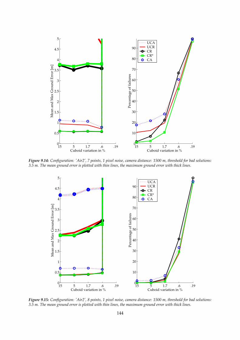
15 5 1.7 .6 .190

0.5

1

1.5

2

2.5

3

3.5

4

4.5

5

Cuboid variation in %

Mea

n an

d M

ax G

roun

d Er

ror

[m]

15 5 1.7 .6 .190

10

20

30

40

50

60

70

80

90

Cuboid variation in %

Perc

enta

ge o

f fai

lure

s

UCAUCRCRCR*CA

Figure 9.14: Configuration: ’Air2’, 7 points, 1 pixel noise, camera distance: 1500 m, threshold for bad solutions:3.5 m. The mean ground error is plotted with thin lines, the maximum ground error with thick lines.

15 5 1.7 .6 .190

0.5

1

1.5

2

2.5

3

3.5

4

4.5

5

Cuboid variation in %

Mea

n an

d M

ax G

roun

d Er

ror

[m]

15 5 1.7 .6 .190

10

20

30

40

50

60

70

80

90

Cuboid variation in %

Perc

enta

ge o

f fai

lure

s

UCAUCRCRCR*CA

Figure 9.15: Configuration: ’Air2’, 8 points, 1 pixel noise, camera distance: 1500 m, threshold for bad solutions:3.5 m. The mean ground error is plotted with thin lines, the maximum ground error with thick lines.

144

15 5 1.7 .6 .190

0.5

1

1.5

2

2.5

3

3.5

4

4.5

5

Cuboid variation in %

Mea

n an

d M

ax G

roun

d Er

ror

[m]

15 5 1.7 .6 .190

10

20

30

40

50

60

70

80

90

Cuboid variation in %

Perc

enta

ge o

f fai

lure

s

UCAUCRCRCR*CA

Figure 9.16: Configuration: ’Air2’, 10 points, 1 pixel noise, camera distance: 1500 m, threshold for bad solutions:3.5 m. The mean ground error is plotted with thin lines, the maximum ground error with thick lines.

15 5 1.7 .6 .190

0.5

1

1.5

2

2.5

3

3.5

4

4.5

5

Cuboid variation in %

Mea

n a

nd

Max

Gro

un

d E

rro

r [m

]

15 5 1.7 .6 .190

10

20

30

40

50

60

70

80

Cuboid variation in %

Per

cen

tag

e o

f fa

ilu

res

UCAUCRCRCR*CA

Figure 9.17: Configuration: ’Air2’, 15 points, 1 pixel noise, camera distance: 1500 m, threshold for bad solutions:3.5 m. The mean ground error is plotted with thin lines, the maximum ground error with thick lines.

145

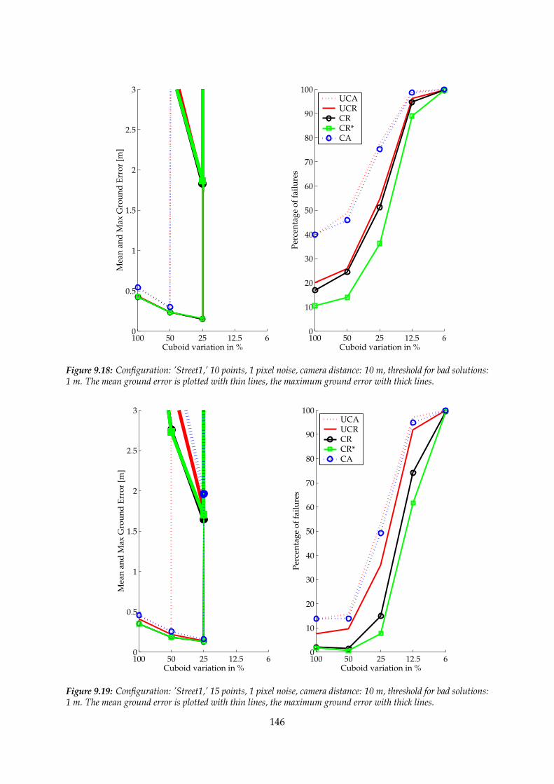
100 50 25 12.5 60

0.5

1

1.5

2

2.5

3

Cuboid variation in %

Mea

n an

d M

ax G

roun

d Er

ror

[m]

100 50 25 12.5 60

10

20

30

40

50

60

70

80

90

100

Cuboid variation in %

Perc

enta

ge o

f fai

lure

s

UCAUCRCRCR*CA

Figure 9.18: Configuration: ’Street1,’ 10 points, 1 pixel noise, camera distance: 10 m, threshold for bad solutions:1 m. The mean ground error is plotted with thin lines, the maximum ground error with thick lines.

100 50 25 12.5 60

0.5

1

1.5

2

2.5

3

Cuboid variation in %

Mea

n a

nd

Max

Gro

un

d E

rro

r [m

]

100 50 25 12.5 60

10

20

30

40

50

60

70

80

90

100

Cuboid variation in %

Per

cen

tag

e o

f fa

ilu

res

UCAUCRCRCR*CA

Figure 9.19: Configuration: ’Street1,’ 15 points, 1 pixel noise, camera distance: 10 m, threshold for bad solutions:1 m. The mean ground error is plotted with thin lines, the maximum ground error with thick lines.

146

100 50 25 12.5 60

0.5

1

1.5

2

2.5

3

Cuboid variation in %

Mea

n an

d M

ax G

roun

d Er

ror

[m]

100 50 25 12.5 60

10

20

30

40

50

60

70

80

90

100

Cuboid variation in %

Perc

enta

ge o

f fai

lure

s

UCAUCRCRCR*CA

Figure 9.20: Configuration: ’Street1,’ 20 points, 1 pixel noise, camera distance: 10 m, threshold for bad solutions:1 m. The mean ground error is plotted with thin lines, the maximum ground error with thick lines.

100 50 25 12.5 60

0.5

1

1.5

2

2.5

3

Cuboid variation in %

Mea

n an

d M

ax G

roun

d Er

ror

[m]

100 50 25 12.5 60

10

20

30

40

50

60

70

80

90

100

Cuboid variation in %

Perc

enta

ge o

f fai

lure

s

UCAUCRCRCR*CA

Figure 9.21: Configuration: ’Street1,’ 25 points, 1 pixel noise, camera distance: 10 m, threshold for bad solutions:1 m. The mean ground error is plotted with thin lines, the maximum ground error with thick lines.

147

100 50 25 12.5 60

0.5

1

1.5

2

2.5

3

Cuboid variation in %

Mea

n a

nd

Max

Gro

un

d E

rro

r [m

]

100 50 25 12.5 60

10

20

30

40

50

60

70

80

90

100

Cuboid variation in %

Per

cen

tag

e o

f fa

ilu

res

UCAUCRCRCR*CA

Figure 9.22: Configuration: ’Street2,’ 10 points, 1 pixel noise, reference distance: 5.7 m, threshold for bad solu-tions: 1 m. The mean ground error is plotted with thin lines, the maximum ground error with thick lines.

100 50 25 12.5 60

0.5

1

1.5

2

2.5

3

Cuboid variation in %

Mea

n an

d M

ax G

roun

d Er

ror

[m]

100 50 25 12.5 60

10

20

30

40

50

60

70

80

90

Cuboid variation in %

Perc

enta

ge o

f fai

lure

s

UCAUCRCRCR*CA

Figure 9.23: Configuration: ’Street2,’ 15 points, 1 pixel noise, reference distance: 5.7 m, threshold for bad solu-tions: 1 m. The mean ground error is plotted with thin lines, the maximum ground error with thick lines.

148

100 50 25 12.5 60

0.5

1

1.5

2

2.5

3

Cuboid variation in %

Mea

n an

d M

ax G

roun

d Er

ror

[m]

100 50 25 12.5 60

10

20

30

40

50

60

70

80

90

Cuboid variation in %

Perc

enta

ge o

f fai

lure

s

UCAUCRCRCR*CA

Figure 9.24: Configuration: ’Street2,’ 20 points, 1 pixel noise, reference distance: 5.7 m, threshold for bad solu-tions: 1 m. The mean ground error is plotted with thin lines, the maximum ground error with thick lines.

100 50 25 12.5 60

0.5

1

1.5

2

2.5

3

Cuboid variation in %

Mea

n an

d M

ax G

roun

d Er

ror

[m]

100 50 25 12.5 60

10

20

30

40

50

60

70

80

90

Cuboid variation in %

Perc

enta

ge o

f fai

lure

s

UCAUCRCRCR*CA

Figure 9.25: Configuration: ’Street2,’ 25 points, 1 pixel noise, reference distance: 5.7 m, threshold for bad solu-tions: 1 m. The mean ground error is plotted with thin lines, the maximum ground error with thick lines.

149

100 50 25 12.5 6.30

0.005

0.01

0.015

0.02

0.025

0.03

0.035

0.04

0.045

0.05

Cuboid variation in %

Mea

n a

nd

Max

Gro

un

d E

rro

r [m

]

100 50 25 12.5 6.30

10

20

30

40

50

60

70

80

90

Cuboid variation in %

Per

cen

tag

e o

f fa

ilu

res

UCAUCRCRCR*CA

Figure 9.26: Configuration: ’Tetra’, 10 points, 10 pixel noise, camera distance: 3 m, threshold for bad solutions:0.25 m.; cf. figure 9.8. The mean ground error is plotted with thin lines, the maximum ground error with thicklines.

150

50 25 12.5 6.3 3.10

0.5

1

1.5

2

2.5

3

3.5

4

4.5

5

Cuboid variation in %

Mea

n a

nd

Max

Gro

un

d E

rro

r [m

]

50 25 12.5 6.3 3.10

5

10

15

20

25

30

35

40

45

Cuboid variation in %

Per

cen

tag

e o

f fa

ilu

res

UCAUCRCRCR*CA

Figure 9.27: Configuration: ’Air1’, 10 points, 10 pixel noise, camera distance: 1500 m, threshold for bad solutions:35 m; cf. figure 9.12. The mean ground error is plotted with thin lines, the maximum ground error with thick lines.

50 25 12.5 6.3 3.10

0.5

1

1.5

2

2.5

3

3.5

4

4.5

5

Cuboid variation in %

Mea

n a

nd

Max

Gro

un

d E

rro

r [m

]

50 25 12.5 6.3 3.10

5

10

15

20

25

30

35

Cuboid variation in %

Per

cen

tag

e o

f fa

ilu

res

UCAUCRCRCR*CA

Figure 9.28: Configuration: ’Air2’, 10 points, 10 pixel noise, camera distance: 1500 m, threshold for bad solutions:35 m; cf. figure 9.16. The mean ground error is plotted with thin lines, the maximum ground error with thick lines.

151

100 50 25 12.5 60

0.5

1

1.5

2

2.5

3

Cuboid variation in %

Mea

n a

nd

Max

Gro

un

d E

rro

r [m

]

100 50 25 12.5 60

10

20

30

40

50

60

70

80

90

100

Cuboid variation in %

Per

cen

tag

e o

f fa

ilu

res

UCAUCRCRCR*CA

Figure 9.29: Configuration: ’Street1,’ 25 points, 2 pixel noise, camera distance: 10 m, threshold for bad solutions:1 m; cf. figure 9.21. The mean ground error is plotted with thin lines, the maximum ground error with thick lines.

100 50 25 12.5 60

0.5

1

1.5

2

2.5

3

Cuboid variation in %

Mea

n a

nd

Max

Gro

un

d E

rro

r [m

]

100 50 25 12.5 60

10

20

30

40

50

60

70

80

90

100

Cuboid variation in %

Per

cen

tag

e o

f fa

ilu

res

UCAUCRCRCR*CA

Figure 9.30: Configuration: ’Street2,’ 25 points, 2 pixel noise, reference distance: 2.85 m, threshold for bad solu-tions: 1 m; cf. figure 9.25. The mean ground error is plotted with thin lines, the maximum ground error with thicklines.

152

The algebraic minimizations, ’UCA’ and ’CA’, should in general produce larger ground errorsand should breakdown earlier than the reprojection methods, ’UCR’ and ’CR’. Methods thatneglect the internal constraints of the tensor should also perform worse than the methods thatconsider them. Therefore the direct linear solution ’UCA’ is expected to be at the low end, andthe constrained method minimizing reprojection error ’CR’ is expected to be at the high end ofthe performances.

Further, we compare the plots with 1 pixel noise in the images of section 9.2.1 with the corre-sponding plots with larger noise of section 9.2.2.

9.3.1 Configuration ’Tetra’

The figures 9.6 – 9.9 on the pages 140 and 141 show the plots of the configuration ’Tetra’ basedon image noise of 1 pixel. The cuboid compressions are given in percent of the camera distanceof 3 m.

Ground Error: Looking at the left plot in each of these figures, we see that up including 8points the unconstrained computation minimizing reprojection error ’UCR’ performs betterthan any algebraic computation (’UCA’ and ’CA’); which indicates the benefit of minimizingreprojection error. From 10 points onwards all five computation methods (’UCA’, ’UCR’, ’CR’,’CR*’, ’CA’) produce practically the same curves for the mean and maximum ground errors; i.e.even the simple direct linear solution ’UCA’ performs equally well to the constrained method’CR’ minimizing reprojection error.

Flatness: Looking at the right plot in each of these figures, we see that from 7 points onwardsthe percentage of bad solutions is slightly smaller for the reprojection methods ’UCR’ and ’CR’than for the algebraic methods ’UCA’ and ’CA’, whereas there is almost no difference in thebad solutions between considering or neglecting the constraints. For 7 points and flatness25% the reprojection methods initialized by the direct linear solution deviates from the ’CR*’solution, which is initialized by the true tensor; this indicates that the direct linear solution canbe insufficient to initialize the iterative methods. For 10 points and 15 points all methods showthe same minimum thickness of 2.8% and 0.9% respectively.

Noise in the images: By comparing the plots based on 10 points with 1 and 10 pixel noisein the images (figure 9.8 on page 141 and figure 9.26 on page 150), we see that the mean andmaximum ground errors and the minimum thickness of the computations are practically scaledby the ratio of the noise in the images. Therefore, at least for the noise-range considered here,the results depend linearly on the noise in the images.

9.3.2 Configuration ’Air1’

The figures 9.10 – 9.13 on the pages 9.10 on page 142 and 9.13 on page 143 show the plots ofthe configuration ’Air1’ based on image noise of 1 pixel. The cuboid compressions are given inpercent of the camera distance of 1500 m.

153

Ground Error: Looking at the left plot in each of these figures, we see that up including 9points the unconstrained computation minimizing reprojection error ’UCR’ performs betterthan any algebraic computation (’UCA’ and ’CA’); which indicates the benefit of minimizingreprojection error. From 10 points onwards all five computation methods (’UCA’, ’UCR’, ’CR’,’CR*’, ’CA’) produce practically the same curves for the mean ground errors; i.e. even the sim-ple direct linear solution ’UCA’ performs equally well to the constrained method ’CR’ mini-mizing reprojection error. The maximum ground error for the algebraic methods is still larger,but from 15 points onwards mean and maximum error for all methods are identical.

Flatness: Looking at the right plot in each of these figures, we see that for 8 points the curvesof the bad solutions for all methods have values different from zero even for 15% flatness. For8 and 9 points all methods relying on the initialization through the direct linear solution ’UCA’have larger percentage of bad solutions than the ’CR*’ method. Again, this shows that forsmall number of points the ’UCA’ can be insufficient to initialize the iterative methods. From10 points onwards, however, all methods are identical in their behavior concerning the badsolutions and show the same minimum thickness, which is 5%, 1.7% and 0.6% for 9, 10 and 15points respectively.

Noise in the images: By comparing the plots based on 10 points with 1 and 10 pixel noisein the images (figure 9.12 on page 143 and figure 9.27 on page 151), we see that the mean andmaximum ground errors and the minimum thickness of the computations are practically scaledby the ratio of the noise in the images. Therefore, at least for the noise-range considered here,the results depend linearly on the noise in the images.

9.3.3 Configuration ’Air2’

The figures 9.14 – 9.17 on the pages 9.14 on page 144 and 9.17 on page 145 show the plots ofthe configuration ’Air2’ based on image noise of 1 pixel. The cuboid compressions are given inpercent of the camera distance of 1500 m.

Ground Error: Looking at the left plot in each of these figures, we see that up including 10points the unconstrained computation minimizing reprojection error ’UCR’ performs betterthan any algebraic computation (’UCA’ and ’CA’); which indicates again the benefit of minimiz-ing reprojection error. From 10 points onwards all five computation methods (’UCA’, ’UCR’,’CR’, ’CR*’, ’CA’) produce practically the same curves for the mean ground errors; i.e. even thesimple direct linear solution ’UCA’ performs equally well to the constrained method ’CR’ min-imizing reprojection error. The maximum ground error for the algebraic methods is still larger,but from 15 points onwards mean and maximum error for all methods are identical. So, exceptthat ’Air2’ performs better than ’Air1’ for small number of points, from 10 points onwards both’Air’ configurations perform identically.

Flatness: Looking at the right plot in each of these figures, we see that for 7 points the curvesof the bad solutions are to some extent the same for all methods, except for ’CR*’, which issignificantly better; this indicates again that the direct linear solution for seven points can be

154

not sufficient to initialize the iterative methods. From 10 points onwards, however, all meth-ods are identical in their behavior concerning the bad solutions and show the same minimumthickness, which then only depends on the number of point correspondences.

Noise in the images: By comparing the plots based on 10 points with 1 and 10 pixel noisein the images (figure 9.16 on page 145 and figure 9.28 on page 151), we see that the mean andmaximum ground errors and the minimum thickness of the computations are practically scaledby the ratio of the noise in the images. Therefore, at least for the noise-range considered here,the results depend linearly on the noise in the images.

9.3.4 Configuration ’Street1’

The figures 9.18 – 9.21 on the pages 9.18 on page 146 and 9.21 on page 147 show the plots of theconfiguration ’Street1’ based on image noise of 1 pixel. The cuboid compressions are given inpercent of the camera distance of 10 m.

Ground Error: Looking at the left plot in each of these figures, we see that from 10 pointsonwards all methods show practically the same curves of mean and maximum error; so thereis practically no gain in accuracy in computing ’CR’ compared to ’UCA’.

Flatness: The right plot of the bad solutions, however, shows a radically different picture asthe percentage of bad solutions for the two algebraic methods ’UCA’ and ’CA’ always lie clearlyabove all reprojection methods; although the difference gets smaller with increasing number ofpoints.

Noise in the images: By comparing the plots based on 25 points with 1 and 2 pixel noisein the images (figure 9.21 on page 147 and figure 9.29 on page 152), we see that the meanand maximum ground errors of the computations are to some extent scaled by the ratio of thenoise in the images. This also holds true for the percentage of bad solutions. However, for 1pixel noise the smallest percentage of bad solutions is 0% (for a cuboid compression of 25%),whereas for 2 pixel noise the smallest percentage is about 10% (for a cuboid compression of50%). This shows that due to the weak image geometry the impact of the image noise on thecritical planarity is much stronger than for the previous configurations.

Additional note: The reason for almost identical ground error curves between algebraic andreprojection methods is caused by the large number of 10 – 25 points, and not due to somehidden properties of the algebraic methods. For smaller number of points the algebraic meth-ods are practically useless concerning accuracy. Since we can see that even for 10 points anymethod produces bad solutions with a percentage of at least 20 %, the high number of pointswas selected to show their requirement for a reliable, i.e. not bad, solution. So the ground errorplots of the algebraic methods should be understood as: When the algebraic solution is good, it iscomparable to the reprojection method, however, the chances of getting a good result from an algebraicmethod is much smaller than for a reprojection method.

155

Note also the strange course of the ground error plots, which gets better with increasing flat-ness. This behavior is explained by the way the cuboid is compressed. This is done in directionto the images by fixing the side of the cuboid, which faces the images. Therefore all points movecloser to the images and the mean intersection angle of corresponding projection rays gets larger.Consequently the accuracy of the determined points also becomes better.

9.3.5 Configuration ’Street2’

The figures 9.22 – 9.25 on the pages 9.22 on page 148 and 9.25 on page 149 show the plots of theconfiguration ’Street2’ based on image noise of 1 pixel. The cuboid compressions are given inpercent of a reference distance of 2.85 m; see figure 9.5.

Ground Error: Looking at the left plot in each of these figures, we see that from 10 pointsonwards all reprojection methods are clearly distinct from the algebraic methods (see also thefollowing additional note 1), while there is no difference between the constrained and uncon-strained methods of the same minimization.

Flatness: The plot of the bad solutions shows, that – similar to ’Street1’ – the percentage of badsolutions for the two algebraic methods ’UCA’ and ’CA’ always lie clearly above all reprojectionmethods; although the difference gets smaller with increasing number of points.

Noise in the images: By comparing the plots based on 25 points with 1 and 2 pixel noise inthe images (figure 9.25 on page 149 and figure 9.30 on page 152), we see that, similar to ’Street1’,the mean and maximum ground errors of the computations are also to some extent scaled bythe ratio of the noise in the images. This also holds true for the percentage of bad solutions.Opposed to ’Street1’, however, the smallest percentage of bad solutions is 0% for both 1 and 2pixel noise; namely for the cuboid compression of 25% and 50% respectively. For 2 pixel noiseon both sides of this minimal thickness of 50% the percentage of bad solutions quickly raises.So here again due to the weak geometry the impact of the image noise on the critical planarityis stronger than for the configurations with stable geometry; i.e. ’Tera’ and ’Air’.

Additional note 1: From the way the ground error curve of the algebraic methods progressesfrom 10 to 25 points without ever reaching the curve of the reprojection methods, we see thatthere is a clear bias between these two kinds of minimizations. This is opposed to ’Street1’,where already for 10 points practically no difference between both minimizations could beobserved.

This bias is caused by the nature of the algebraic error, which is the deviation from zero on theright side of the homogenous point-trilinearities. For each corresponding triple of image pointsx′, x′′, x′′′ four point-trilinearities (7.29) on page 76 are set up. Each of these four trilinearitiescan be represented as x′>λ′jk = 0, j, k = 1, 2. The line λ′jk in image Ψ1 is the projection of a3D line, which is created by the intersection of the back-projection of the lines σ ′′

j and σ ′′′k ; cf.

section 7.3 and figure 7.7 on page 76.

Due to the special geometry of the ’Street’-configurations, the lines λ′12 and λ′21 run approxi-mately radially from the principal point of image Ψ1 to the point x′. This holds true for image

156

Ψ1 in both configurations ’Street1’ and ’Street2’. The bias in the algebraic minimization for’Street1’ is caused by the distribution of the points x′ in image Ψ1, which is totaly different to’Street2’.

In ’Street1’ the cuboid is compressed in direction of the basis of the images, therefore the distri-bution area of the points x′ stays practically the same for all cuboid compressions. In ’Street2’the cuboid is compressed orthogonally to the basis of the images, in direction to the street,therefore the distribution area of the points x′ is limited to the lower half of image Ψ1; seefigure 9.31.

Figure 9.31: The image Ψ1 of configuration ’Street1’ (left) and ’Street2’ (right), with the lines λ′jk drawn in fourrepresentative points. In image Ψ1 of ’Street1’ the lines λ′12 and λ′21 are not limited in their direction, whereasin image Ψ1 of ’Street2’ these lines, and partly the lines λ′11, have all approximately the same direction (i.e. they′c-direction).

During the algebraic minimization the deviations on the right side of the trilinearities x′>λ′jk = 0are minimized. These trilinearities represent the incidence relation between the point x′ and theline λ′jk. Therefore the right side of these trilinearities corresponds to the orthogonal distance ofthe point x′ to the line λ′jk, however, scaled by the norm of the homogenous part of λ′jk. Now, aswe can see from figure 9.31 for the configuration ’Street2’, the lines λ′12, λ′21, and partly the linesλ′11, have all approximately the same direction (i.e. the y′c-direction). Therefore the contributionof the error component orthogonal to this direction (i.e. the x′c-direction) to the total algebraicerror is almost three times higher than for the y′c-direction.

These different, unjustified, weights of the four point-trilinearities of ’Street2’ are the reason forthis bias. For ’Street1’ the lines λ′12 and λ′21 are not limited in their direction as the points x′ arescattered in the whole image area.

The algebraic error corresponds to the distance of the point x′ to the line λ′jk, scaled by the normof the homogenous part of λ′jk. The scale of λ′jk depends on the coordinates of the points x′′ andx′′′ in the other images. So there could be an additional source of bias in the algebraic error dueto the scale difference between the Euclidian coordinates, which can be some 1000 pixels, andthe homogenous extension of 1. Because of the conditioning following section 3.7 on page 27,however, this bias should be eliminated to a large extent, as all image points are translated totheir centroid and are appropriately scaled afterwards. This conjecture is also backed by theresults of ’Street1’, which does not show this kind of bias.

157

Additional note 2: A strange course of the ground error plots, which gets better with increas-ing flatness, can be observed, similar to ’Street1’. The reason for this course, however, is differ-ent to ’Street1’, where it was caused by the increasing mean intersection angle of correspondingprojection rays due to the cuboid compression. Here the mean intersection angle stays moreor less the same, since the depth of the cuboid remains fixed and only its height is flattened.For ’Street2’ the improvement is caused by the increasing distance of the points to the commonbasis of the three images, which cuts right through the middle of the uncompressed cuboid.For object points on this basis the intersection angle of corresponding projection rays is zeroand therefore the object point is undeterminable1. According to this, in the vicinity to the basisthe intersection angle will be very small, resulting in very badly determined object points. Thepercentage of such points decreases as the cuboid for ’Street2’ is compressed. Consequentlythe mean and maximum ground error get smaller.

Since the mean intersection angle for ’Street2’ does not increase that much as it does for ’Street1’,the actual values of the ground errors is higher than for ’Street1’.

9.4 Summary

The expectations stated in the beginning of section 9.3 on page 139 are practically confirmed,however the direct linear solution performed much better than presumed. We can summarizethe results of the examples with 1 pixel noise in the images in the following way:

• The ground errors obtained for the different computation methods tend to be the same

– for a particular image configuration, if the number of point correspondences increases, and

– for a particular number of point correspondence, if the stability of the image geometry in-creases.

Therefore, from 10 points onwards for ’Tetra’, ’Air1’ and ’Air2’, and from 25 points onwardsfor ’Street1’ and ’Street2’, all computation methods return practically the same result; i.e.then the direct linear solution is equivalent to the constrained computation minimizing reprojectionerror.

• For small numbers of point correspondences, ≤ 8 for the stable configurations ’Tetra’, ’Air1’and ’Air2’ and for the unstable configurations ’Street1’ and ’Street2’ in general, the uncon-strained minimization of reprojection error generally performed better than any algebraic(constrained or unconstrained) minimization. Therefore, the benefit of minimizing only repro-jection error, is larger than of considering only the constraints.

• The algebraic minimizations can produce a bias for certain lopsided configurations,i.e. ’Street2’, due to the incorrect weighting of the trilinearities.

• Concerning the impact of the minimum thickness of the cuboid on the various computationmethods, we can say

1For the preparation of these examples we were aware of this fact and therefore the number of points place inthe cuboid along each direction is even, because for an odd number, points exactly on the basis would have beencreated.

158

– for image configurations with strong geometry, i.e. ’Tetra’, ’Air1’ and ’Air2’, the minimumthickness is practically independent on the computation method of the tensor, and be-comes smaller for larger numbers of point correspondences.

– for image configurations with weak geometry, i.e. ’Street1’ and ’Street2’, the minimumthickness is larger for the algebraic methods and smaller for the reprojection methods,where the consideration of the internal constraints adds a significant additional benefit;and for larger numbers of point correspondences the minimum thickness also gets smallergenerally.

• Depending on the number of point correspondences, the computation of the trifocal tensorwas still successful for the minimum thickness of the cuboid given in table 9.6; afterwards itfailed. Because of the discrete cuboid compressions the actual minimum thickness is smallerthan the presented values; i.e. if the percentage of ’bad’ solutions for one compression iszero and for the next it is non-zero, then the actual minimum thickness lies somewhere inbetween.

number of pointsconfiguration

8 10 15

’Tetra’ 8.3 % 2.8 % 0.9 %camera distance approx. 3 m

’Air1’ >15 % 1.7 % 0.6 %camera distance approx. 1500 m

’Air2’ 5 % 1.7 % 0.6 %camera distance approx. 1500 m

number of pointsconfiguration

15 20 25

’Street1’ 50 % 50 % 25 %camera distance approx. 10 m

’Street2’ 50 % 25 % 12.5 %reference distance approx. 2.85 m

Table 9.6: Minimum thickness in percent of the camera distance for which the computation of the trifocal tensorwas still successful. For the configurations ’Tetra’, ’Air1’ and ’Air2’ the given values hold for any computa-tion method, whereas for the two ’Street’ configurations they hold only for the constrained method minimizingreprojection error.

By comparing the plots for the configurations ’Tetra’, ’Air1’ and ’Air2’ based on 1 pixel noise inthe images with the respective plots based on 10 pixel noise, we see that the ground errors andthe minimum thickness of the computations are practically scaled by the ratio of the injectednoise. Therefore, using 10 as a representative number of points for the configurations ’Tetra’,’Air1’ and ’Air2’, we can summarize the mean and maximum ground error and the minimumthickness with the following formulas (distance D to object, noise σ in the image, principaldistance c):

159

’Tetra’:

Mean ground error = 2D ·σ

c

Max ground error = 9D ·σ

c

Minimum thickness ≤ 98D ·σ

c

’Air1’:

Mean ground error = 4D ·σ

c

Max ground error = 23D ·σ

c

Minimum thickness ≤ 340D ·σ

c

’Air2’:

Mean ground error = 3D ·σ

c

Max ground error = 20D ·σ

c

Minimum thickness ≤ 340D ·σ

c

We can use the symbol ’≤’, because of the discrete cuboid compressions. Also note that the prin-cipal distance is only included in these formulas to be independent on the units in the imagespace, and that the formulas may not be very correct for totally different principal distances forthe same cameras. Here the principal distance for ’Air1’ and ’Air2’ is 20000 pixel and for ’Tetra’it is 3500 pixel.

Similar formulas for the two ’Street’ configuration are not given, since due to the very weakgeometry the ground error depends highly on the cuboid compression, with better groundaccuracies for thinner cuboids. Further, since for higher noise levels than 2 pixel no usefulresults were obtained, it can be deduced that the influence of the noise level is more crucial,which further prevents the derivation of general formulas.

Since the ’Air1’ configuration is probably the most relevant for practical applications, we cantake a closer look at the distribution of the planer and height components of the errors of thisconfiguration; using 10 points and 1 pixel noise. From figure 9.32 on the following page wesee that the mean planar error and the mean height error are about (12 cm/50 cm) for the’CR’ method and (17 cm/68–75 cm) for the ’UCA’ method. For the same configuration butusing calibrated instead of uncalibrated images, we can adapt the formulas of [Kraus 1993] andobtain the planar error as 1[pixel] · 1500[m]/20000[pixel] = 7.5 cm and the height error as0.15h · 1500[m] = 23.5 cm. Therefore, the constrained determination of the trifocal tensor isapproximately 2 times worse and the direct linear solution is approximately 3 times worse.In general, however, the relative orientation of the three images obtained from both methods,especially from the direct linear solution, is a sufficient good approximation to initialize a finalbundle block adjustment during which the known interior orientation of the images can befully exploited.

160

15 5 1.7 .6 .190

0.1

0.2

0.3

0.4

0.5

0.6

0.7

0.8

0.9

1

Cuboid variation in %

Mea

n a

nd

Max

Gro

un

d E

rro

r [m

]

15 5 1.7 .6 .190

10

20

30

40

50

60

70

80

90

Cuboid variation in %

Per

cen

tag

e o

f fa

ilu

res

UCAUCRCRCR*CA

Figure 9.32: Separation of the mean ground errors in planar component (thin line) and height component (thickline); 1000 realizations, Configuration: ’Air1’, 10 points, 1 pixel noise, camera distance: 1500 m, threshold for badsolutions: 3.5 m.

Conclusion. Summing it up, if the image geometry is not too bad and at least 10 correspond-ing points are used, then the simple direct linear method ’UCA’ for determining the trifocaltensor, which neglects the internal constraints and minimizes reprojection error, practicallyperforms equal to the constrained method ’CR’, which minimizes reprojection error. Conse-quently, if the trifocal tensor is only computed to obtain approximations for the orientationparameters of a bundle block adjustment, the direct linear solution ’UCA’ is usually sufficient.However, if a general routine for providing such initial values is requested, which does nothave any restrictions on the image geometry and also handles weak configurations, then theGauß-Helmert model ’CR’ minimizing reprojection error must be used.

161

Chapter 10

Conclusion

The topic of this thesis is the trifocal tensor, which describes the relative orientation (or epipo-lar geometry) of three uncalibrated images. It is a homogenous valence-(1,2) tensor, which meansthat it can be represented as a 3×3×3 cube of number. The trifocal tensor is of particular inter-est because it can be determined linearly from corresponding points or lines in the three images.Consequently it provides a tool to determine the relative orientation of three images without requiringapproximate values. This relative orientation can be further used as initial values in a subsequentbundle block adjustment.

Each triple of points provides 4 linear equations, called trilinearities, in the tensor elementsand each corresponding triple of lines provides 2 such linear equations; therefore at least 7points, 13 lines or a proper combination are needed for a direct linear solution of the trifocaltensor. To obtain a unique solution it is important that the corresponding image features donot arise from a critical configuration. The probability of running into such configurations ismuch smaller than for two images and the fundamental matrix. However, if all correspondingimage features arise from a common plane the direct solution fails. This is due to the fact thatthe images are considered uncalibrated.

10.1 Summary

Although the point and line trilinearities allow a simple direct linear solution of the trifocal ten-sor, there are, however, some drawbacks associated with this linear solution. The trifocal tensoris made up of 27 elements, but it only has 18 degrees of freedom. Consequently its elementshave to satisfy 8 internal constraints, besides the fixing of the tensor’s scale, to represent a validtrifocal tensor. These constraints are in generally not satisfied by the direct linear solution. An-other drawback is that the direct linear solution does not minimize the errors in the originalpoint and line measurements (so-called reprojection error) but some other quantities (so-calledalgebraic error).

Because of these drawbacks, errors in the tensor elements will be induced and therefore theobtained relative orientation may be not sufficient to initialize a subsequent bundle block ad-justment. These drawbacks can be prevented by determining a valid trifocal tensor by mini-mizing reprojection error. The so-called Gauss-Helmert model provides a general environment

162

for such constrained adjustment tasks. The determination of a valid trifocal tensor in the Gauß-Helmert model can be done basically in two ways: By parameterizing the tensor using its 27elements and introducing the 8 internal constraints together with the scale fixing, or by usingan alternative parameterization for the trifocal tensor that has 18 degrees of freedom.

Several sets of constraints and alternative parameterizations have been proposed over the yearsand we reviewed the most important ones in the sections 7.6 on page 93 and 8.3 on page 112respectively. In this thesis we also derived two new sets of constraints and gave a simplegeometric interpretation for them. We also found a new alternative parameterization for thetrifocal tensor.

For computing a valid trifocal tensor by minimizing reprojection error in the Gauß-Helmertmodel it is important to have a consistent representation for the trifocal tensor. The parameter-ization using the projection matrices proposed in [Hartley 1994a] and reviewed in section 8.3.1on page 113 is the simplest way for such a consistent representation. This parameterizationis applicable as long as (i) not all three projection centers coincide and (ii) the first projectioncenter is different from the other two.

Empirical investigations in section 9 on page 130 showed the difference in computing the trifo-cal tensor by minimizing algebraic error or reprojection error with or without considering theinternal constraints. Further the minimum thickness of the object points was investigated; i.e.what is the minimum deviation of the object points from a common plane, so that the compu-tation is still possible?

The findings can be summarized in the following way: For image configurations with stronggeometry, like in the case of convergent terrestrial images or in the case of aerial images, thedirect linear solution for the trifocal tensor and the valid tensor from the Gauß-Helmert modelminimizing reprojection error are practically the same. Concerning the minimum thicknessunexpected small values were found already for 10 point correspondences. If the number ofpoints increases, then the minimum thickness gets even smaller. For the mentioned configura-tions and 15 point correspondences the computation of the trifocal tensor is still successful fora minimum thickness of the object points of about 1% of the camera distance (normal anglecamera with assumed noise in the images of 1 pixel).

For image configurations with weak geometry, like collinear projection centers with congruentviewing directions, much more point correspondences are required and the direct linear solu-tion fails more often for small thicknesses of the object points than the valid solution from theGauß-Helmert model minimizing reprojection error.

From these empirical investigations we come to the conclusion that minimizing reprojection er-ror and considering the internal constraints is actually not necessary if the image configurationhas a strong geometry – especially if one is only interested in initial values for a subsequentbundle block adjustment. However, if a general tool for providing such initial values is re-quested, which does not have any restrictions on the image geometry and handles also weakconfigurations, then the Gauß-Helmert model minimizing reprojection error must be used.

If n > 3 images are given, then many unrelated trifocal tensors are computed. Before all nimages can be used simultaneously, the individual basis vectors and rotation matrices derivedfrom the unrelated tensors must be transformed into one common system; see section 7.4.6 onpage 91.

163

10.2 Contribution of this thesis

The contribution of this thesis can be divided into a theoretical part, concerning geometry andconstraints of the trifocal tensor, a practical part, concerning the computation of the trifocaltensor, and an empirical part, concerning the necessity of computing a valid trifocal tensor byminimizing reprojection error as opposed to the direct linear solution.

Geometry and constraints of the trifocal tensor. Two new minimal sets of constraints werederived in section 7.6.3 on page 96. A set of constraints is termed minimal if it is made up ofexactly 8 constraints.

For deriving these constraints we reviewed thoroughly the properties of the trifocal tensor bymeans of its tensorial slices, the matrices Ii, J j and Kk; see section 7.2 on page 63.

Using the so-called principal rays, which are the projection rays of the canonical points of animage, we found a simple geometric interpretation for the new set of constraints: The eightconstraints of the trifocal tensor guarantee that the mappings of the principal rays of each image into theother two images are straight and concurrent lines.

Further, we discovered a new parameterization, which uses 20 parameters; see section 8.3.4 onpage 119. Therefore 2 constraints, which fix two scaling ambiguities, need to be considered inthe Gauß-Helmert model. From this parameterization also a very simple minimal parameteri-zation can be derived, which has exactly 18 parameters. These 18 parameters have a simplegeometric interpretation; see proposition 8.1 on page 120.

Minimal parameterizations have the advantage that their implementation requires no addi-tional constraints, however, generally more than one minimal parameterization are required torepresent all possible trifocal tensors. In case of the new minimal parameterizations 81 mapsfrom the set of all possible trifocal tensors to the new minimal parameterization exist. This is,however, still less than the number of maps for the minimal parameterization of [Papadopouloand Faugeras 1998], which is 59.049.

Computation of the trifocal tensor. Using the trilinearities of points and lines in section 7.3on page 74 the 27 elements of the trifocal tensor can be computed linearly. This direct linearsolution, however, has the drawbacks, that the internal constraints are not satisfied and thatalgebraic error is minimized instead of reprojection error. These drawbacks can be avoided if avalid trifocal tensor is computed in the Gauß-Helmert model by minimizing reprojection error.This can be done basically in two ways: By parameterizing the tensor using its 27 elementsand introducing the 8 internal constraints together with the scale fixing; or by using an alter-native, minimal or non-minimal, parameterization for the trifocal tensor that has 18 degrees offreedom.

However, the method of introducing the 8 internal constraints is not recommended, becauseall sets of constraints reviewed in section 7.6 on page 93, including the new ones, suffer fromone of the following reasons; cf. section 8.3.5 on page 124: The constraints are too complex tobe implemented in the Gauß-Helmert model, they are not minimal (i.e. > 8) or they are notvalid for all image configurations. Also the minimal parameterizations reviewed in section 8.3on page 112 can not be recommended for realization in the Gauß-Helmert model due to theircomplexity, which is primarily caused by the many case differentiations involved.

164

Actually, only the new parameterization of section 8.3.4 on page 119, using 20 parameters and 2constraints, and the parameterization using the projection matrices of section 8.3.1 on page 113,using 24 parameters and 6 constraints, are relatively simple to be realized in the Gauß-Helmertmodel. The benefit of the parameterization using the projection matrices is that there is only onemap from all trifocal tensors to this parameterization, whereas for the new parameterizationthere are three maps. On the other hand the parameterization using the projection matricesrequires 6 constraints, whereas the new parameterization needs only 2 constraints.

However, since the simplicity of the implementation, i.e. the number of maps, is more impor-tant than the number of required constraints, the parameterization using the projection matrices isthe recommended way to represent a valid trifocal tensor in the Gauß-Helmert model.

Empirical studies. In chapter 9 on page 130 the trifocal tensor is determined by various meth-ods for five different image configurations and for different numbers of corresponding points.Three image configurations, ’Tetra’ (the three projection centers and the object center from atetrahedron), ’Air1’ and ’Air2’ (images from one and two flight strips), represent stable imagegeometries with intersection angles of about 90 and 17 respectively. The other two configu-rations, ’Street1’ and ’Street2’ (three collinear projection centers with congruent viewing direc-tions), have a rather unstable geometry with intersection angles of about 3.

These examples are based on synthetic data and shall demonstrate the differences betweenminimizing algebraic and reprojection error, the effects of considering or neglecting the internalconstraints of the tensor, and the impact of critical configurations; i.e. how close must points lieto the same plane so that the computation fails?

The results from these investigations can be summarized in the following way:

– The differences in the results of the various computation methods vanish for a particularimage configuration if the number of point correspondences increases, and for a particular num-ber of point correspondence if the stability of the image geometry increases. Therefore, from 10points onwards for ’Tetra’, ’Air1’ and ’Air2’, and from 25 points onwards for ’Street1’ and’Street2’, all computation methods return practically the same result; i.e. then the direct linearsolution is equivalent to the constrained computation minimizing reprojection error.

– For small numbers of point correspondences, ≤ 8 for the stable configurations ’Tetra’, ’Air1’and ’Air2’ and for the unstable configurations ’Street1’ and ’Street2’ in general, the uncon-strained minimization of reprojection error generally performed better than any algebraic(constrained or unconstrained) minimization. Therefore, the benefit of minimizing only repro-jection error, is larger than of considering only the constraints.

– The algebraic minimizations can produce a bias for certain lopsided configurations,i.e. ’Street2’, due to the incorrect weighting of the trilinearities.

– Concerning the critical configuration of almost planar object points we can say that for imageconfigurations with stable geometry the minimum thickness, i.e. the minimum deviationfrom a common plane, is practically independent from the computation method of the tensor. Forimage configurations with unstable geometry the minimum thickness strongly depends onminimizing reprojection error and considering the internal constraints.

Generally the minimum thickness becomes smaller if the number of point correspondencesincreases. Therefore, the computation of the trifocal tensor is still successful for the following

165

minimum thickness of the object points, represented in units of the camera distance (normalangle camera with assumed noise in the images of 1 pixel, 15 point correspondences):

· ’Tetra’ (1 pixel = 9 µm): flatness of 1/100,

· ’Air1’ and ’Air2’ (1 pixel = 15 µm): flatness of 6/1000.

Summing it up, if the image geometry is not too bad and at least 10 corresponding pointsare used, then the simple direct linear method for determining the trifocal tensor, which ne-glects the internal constraints and minimizes reprojection error, practically performs equal tothe constrained method, which minimizes reprojection error. Consequently, if the trifocal ten-sor is only computed to obtain approximations for the orientation parameters of a bundle blockadjustment, the direct linear solution is usually sufficient. However, if a general routine forproviding such initial values is requested, which does not have any restrictions on the imagegeometry and also handles weak configurations, then the Gauß-Helmert model minimizingreprojection error must be used.

10.3 Outlook

The following tasks seem worth further investigations:

Calibrated images. In section 8.5 on page 128 the critical configurations for determining thetrifocal tensor are reviewed. If the correspondences arise from points lying on certaincurves in space or in a plane then the trifocal tensor can not be determined uniquely. Thechances of running into a configuration involving those critical curves is rather small,however, point correspondences from a common plane occur very often, especially ifman-made objects are involved. The examples from section 9 showed that the minimumthickness, required to successfully determine the trifocal tensor, depends on the distancebetween camera and object, and the noise in the image. Therefore the problem may inpractise be solved by using larger image scales, however, a certain risk remains, becauseoften the images are taken without considering these critical planarities or approachingthe object is restricted by environmental conditions.

Planar object points constitute a problem because the images are regarded as uncalibratedwhen computing the trifocal tensor. If the the interior orientation of the images is known,then this problem may be solved in general. Empirically we found that the system of thedirect linear solution has rank-21 instead of rank-26. Consequently by applying the inter-nal constraints on this 5-parameter family of direct solutions a certain countable numberof valid trifocal tensors will result and if we further consider the known interior orien-tation parameters, the number of valid trifocal tensors fitting to this interior orientationmay be broken down to a single solution.

Empirical investigations. From the examples in section 9 we derived formulas for the grounderrors and the minimum thickness for certain image configurations depending on thenoise level in the images. These formulas are backed only by two different noise levels,which were considered in the examples, and only one principal distance is used. There-fore an approach, considering different noise levels, various principal distances and otherimage configurations, will result in formulas with a more general validity.

166

Algebraic error. We also saw during the examples, that for geometric stable configurationsusing a certain number of point correspondences the results obtained by minimizing al-gebraic error are very similar to the results of minimizing reprojection error. On the otherhand we also saw that for certain lopsided image configurations the minimizing of alge-braic error produces a bias in the results. A more thorough investigation of the relationship between these two kinds of minimizations may give deeper insights into the behav-ior of minimizing algebraic error during the determination the trifocal tensor.

Lines. One benefit of dealing with the trifocal tensor is its ability to handle points and linesat the same time. During the examples in section 9 we only consider point correspon-dences. Also in the literature primarily points are used in connection with the trifocaltensor. Therefore it is worth investigating the benefits and limitations of considering linecorrespondences with and without additional point correspondences.

Lines have the advantage of occurring frequently in images, especially in industrial scenes.They can be extracted automatically, often with higher accuracy than points; provided thelines are long enough. Line correspondences can be established even if occlusions occurin the images. However, since one single line does not constrain the image geometry asmuch as one single point, many more line correspondences will be necessary to achievethe same accuracy as with a certain number of points.

Distortion. The trifocal tensor so far is embedded in the framework of projective geometry,which does not include non-linear image distortions. If the trifocal tensor is only deter-mined to derive approximations of the image orientations for a subsequent bundle blockadjustment, this limitation should not be of much concern, provided the non-linear dis-tortions are not too large and the points are well distributed. However, if an optimalestimate of the trifocal tensor is wanted, then non-linear distortion parameters have to beincluded in the projective framework. Some strategies can be found in the literature; e.g.[Niini 2000] or [Fitzgibbon 2001].

167

Appendix A

Notation

In this chapter the notation used within this thesis is summarized in detail. Quantities withfixed scale are represented in slanted notation, and homogenous quantities are represented inupright notation.

special symbols

|A| = det(A) the determinant of the matrix A

||A||Frob the Frobenius norm of the matrix A; see definition B.3 on page 175

|x|, |s| the length of a vector x and the absolute value of a scalar s

x∗, λ∗ the dual of a point x and the dual of a line λ

A? the cofactor matrix of the matrix A, which is the transposed of the ad-joint; see equation (B.14) on page 173

<x, y> the inner, or scalar, product of two vectors x and y

dxe smallest integer being equal to or larger than x

lower case Roman font

e′2, e′3the epipoles in image Ψ1 with respect to the images Ψ2 and Ψ3 ; seerelation (6.1) on page 42

ii the ith column of the identity matrix I3; see table 3.1 on page 14

x′, x′′, x′′′ corresponding image points in the images Ψ1, Ψ2 and Ψ3

lower case Greek font

ε′2an epipolar line in image Ψ1 with respect to image Ψ2; see section 6.1.1on page 42

λ′, λ′′, λ′′′ corresponding image lines in the images Ψ1, Ψ2 and Ψ3

κ the eigenvalue of a standard or general eigenvalue problem

π∞ the line at infinity; see section 3.2 on page 11

ρ′31, ρ′32, ρ′33maps of the principal rays R′′′

1 , R′′′2 and R′′′

3 of image Ψ3 into imageΨ1; see proposition 6.4 on page 44

168

upper case Roman or Sans Serif font

A M2M1−1; see equation (7.4) on page 60

Athe Jacobian-matrix of the condition equations, especially in the Gauß-Helmert model, with respect to the unknown parameters; see sec-tion 8.2 on page 109

B M3M1−1; see equation (7.4) on page 60

Bthe Jacobian-matrix of the condition equations in the Gauß-Helmertmodel with respect to the observations; see section 8.2 on page 109

C1 the calibration matrix of image Ψ1; see equation (5.7) on page 35

Cthe Jacobian-matrix of the constraints in the Gauß-Helmert model withrespect to the unknown parameters; see section 8.2 on page 109

E12the essential matrix from image Ψ2 to image Ψ1; see equation (6.11) onpage 46

F12the fundamental matrix from image Ψ2 to image Ψ1; see theorem 6.1 onpage 43

G a general correlation matrix; see definition 3.3 on page 21

GLthe dual correlation induced by the 3D plane L; see proposition 6.10 onpage 54

H a general homography matrix; see definition 3.2 on page 20

HΩthe homography induced by the 3D plane Ω; see proposition 6.7 onpage 50

H∞ the homography induced by the plane at infinity Π∞; see equation(6.17) on page 53

Iithe ith tensorial slice in direction i – a dual line correlation from imageΨ2 to image Ψ3; see proposition 7.1 on page 64

In the identity matrix of dimension n

Ii the ith column of the identity matrix I4

J jthe jth tensorial slice in direction j – a point homography from imageΨ1 to image Ψ3; see proposition 7.5 on page 68

Kkthe kth tensorial slice in direction k – a point homography from imageΨ1 to image Ψ2; see proposition 7.9 on page 71

M1the leftmost 3×3 sub-matrix of the point projection matrix P1; see equa-tion (5.9) on page 36

P1 the point projection matrix of image Ψ1; see equation (5.6) on page 35

IP1, IP2, IP3, IPn the projective spaces of dimension 1, 2, 3 and n

IP2∗ the dual projective spaces of dimension 2

Q1 the line projection matrix of image Ψ1; see proposition 5.1 on page 37

R1 the rotation matrix of image Ψ1; see section 5.2 on page 34

IR2, IR3, IR4, IRn the Euclidian spaces of dimension 2, 3, 4 and n

169

upper case Roman or Sans Serif font

S(·) the axiator, i.e. the operator that returns the cross-product matrix; seeequation (B.8) on page 173

Sred(·) the axiator reduced by one row; see section 3.6 on page 27

S the diagonal matrix of singular values; cf. section B.2 on page 172

U the left orthogonal matrix of singular value decomposition

V the right orthogonal matrix of singular value decomposition

Z1 the projection center of image Ψ1; always represented as a Euclidian vector

upper case Greek font

I(·) the operator that returns a 4×4 matrix, the Plücker matrix, needed forjoining and intersecting 3D entities; see section 3.5 on page 22

Σ(λ′) the projection plane of image line λ′ in image Ψ1; see relation (5.20) onpage 39

I I(·) the operator that returns a 6×4 matrix needed for joining and intersect-ing 3D entities; see section 3.5 on page 22

Π′1, Π′

2, Π′3 the principal planes of image Ψ1

Π∞ the plane at infinity

Ψ1 the first image; see relation (5.13) on page 36

Ω a general plane in 3D space

upper case Calligraphic font

I i the ith column of the identity matrix I6; see table 3.3 on page 20

L a general line in 3D space

N (A) the nullspace of a matrix A

R′1, R′

2, R′3 the principal rays of image Ψ1 see relation (5.18) on page 38

R(A) the range of a matrix A

S(x′) the projection ray of image point x′ in image Ψ1 see relation (5.23) onpage 39

170

Appendix B

Matrix Calculus

This chapter briefly summarizes some concepts of matrix calculus, which are used within thisthesis.

B.1 The eigenvalue problem

Let A be a square matrix of size n×n. Then finding solutions for the scalars κ1,κ2, . . . and thevectors x1, x2, . . . of the equation

Ax = κx (B.1)

is called the (standard) eigenvalue problem. The scalars κi are called the (standard) eigenvaluesand the vectors xi are called the (standard) right eigenvectors of matrix A. The equation x>A =κx> has the same eigenvalues but in general different (standard) left eigenvectors.

The general eigenvalue problem is of the form

Ax = κBx, (B.2)

where B is also of size n×n. The scalars κ are called general eigenvalues and the vectors xare called the general right resp. left eigenvectors. Without any further specification the termeigenvalue problem always refers to the standard case.

Eigenvalues are found as the roots of the characteristic polynomial

det(A−κI) = 0. (B.3)

The multiplicity ai of a root κi of this polynomial is called algebraic multiplicity of the eigen-value κi. The set of eigenvectors x that satisfies (B.1) for a particular eigenvalue κi is calledthe eigenspace of the eigenvalue κi, and its dimension gi = n− rank(A−κiI) is called the geo-metric multiplicity of the eigenvalue κi. Both types of multiplicities are related by the followingimportant inequality; e.g. [Überhuber 1997]

1 ≤ gi ≤ ai. (B.4)

The eigenvalues of a matrix A are related to the determinant and the trace in the following way:

∏κi = det(A), (B.5)

∑κi = trace(A). (B.6)

171

B.2 The singular value decomposition

The singular value decomposition (SVD) of a real matrix A of size m× n is given by

A = USV>, (B.7)

where U and V are orthogonal matrices of size m×m and n× n respectively, andS = diag(σ1,σ2, . . . ,σk) is a diagonal matrix of size m×n and k = min(m, n). The diago-nal elements satisfy the following inequality

σ1 ≥ σ2 ≥ · · · ≥ σr = σr+1 = · · · = σk = 0 with r = rank(A).

These diagonal elements are called singular values of the matrix A and are identical to the pos-itive square-roots of the eigenvalues of A>A and AA>. The column vectors of U are called leftsingular vectors of A and correspond to the eigenvectors of AA>, and the column vectors of Vare called right singular vectors of A and correspond to the eigenvectors of A>A; e.g. [Golub andVanLoan 1996]. The matrices U and V and hence the singular value decomposition are unique,if all singular values have multiplicity 1.

The singular value decomposition is a very useful tool for doing linear algebra – both in a nu-merical and theoretical way; see e.g. [Golub and VanLoan 1996], [Überhuber 1997] or [Hartleyand Zisserman 2001].

For example, the range R(A) and nullspace N (A) of a rank-r matrix A is easily obtained by

R(A) = u1 ∨ u2 ∨ · · · ∨ ur

N (A) = vr+1 ∨ vr+2 ∨ · · · ∨ vn,

where ui and vi denotes the ith column of U and V respectively; see e.g. [Überhuber 1997].

Consequently, the singular value decomposition represents a simple way to solve homogenoussystems of linear equations Ax = 0, which we encounter several times in this thesis. Providedthe system has rank-(n− 1), the unique solution x is obtained by the last column of V ; i.e.N (A) = vn. In case of an over-determined homogenous system (i.e. m > n), the same vectorx = vn, being the left singular vector to the smallest singular value σn, is the solution of

|Ax|2 → min

and |Ax| = σn. See e.g. [Hartley and Zisserman 2001] for further possible usages of the singularvalue decomposition concerning linear least squares problems.

Also the pseudo inverse or Moore-Penrose inverse A+ of a singular matrix A can be obtained easilywith the singular value decomposition:

A+ = VS+U>,

with S+ = diag(1/σ1, 1/σ2, . . . , 1/σr, 0, . . . , 0). The pseudo satisfies the following conditions

AA+A = AA+AA+ = A+

(A+A)> = A+A(AA+)> = AA+ .

172

B.3 The cross product

The cross product of two vectors a = (a1, a2, a3)> and b = (b1, b2, b3)

>, denoted by a×b, re-turns a vector c that is orthogonal to both vectors a and b:

c =

a2b3 − a3b2a3b1 − a1b3a1b2 − a2b1

with c>a = c>b = 0.

Using the so-called axiator S(a), this can also be written as

c = S(a)b,

with

S(a) =

0 −a3 a2a3 0 −a1−a2 a1 0

. (B.8)

In other publications the axiator is represented as [ a ]× ; e.g. [Hartley and Zisserman 2001]. Thefollowing relations involving S(a) are very helpful.

αS(a) + βS(b) = S(αa + βb) (B.9)S(a)S(b) = ba> − a>bI (B.10)

S(a×b) = S(S(a)b) = ba> − ab> (B.11)

S(Ma) = det(M)M−>S(a)M−1, (B.12)

with M regular. The general formulation of (B.12), which holds for any M , is

S(Ma)M = adj(M>)S(a). (B.13)

adj(M) is the adjoint of the matrix M , defined by

adj(M)(i, j) = (−1)i+ j det(M ′ji), (B.14)

where M ′ji denotes the matrix obtained by striking out the jth row and the ith column of M .

So, if M is regular, it holds adj(M) = det(M)M−1. The relation (B.13) is adopted from [Hartleyand Zisserman 2001]; the other relations are obtained by simple computations.

Here are some rules that hold for cross products involving more than two vectors, adaptedfrom [Bronstein and Semendjajew 1991].

a× (b× c) 6= (a× b)× ca× (b× c) = S(a)S(b)c (B.15)(a× b)× c = S(S(a)b)c (B.16)

(a× b)>(c× d) = (a>c)(b>d)− (a>d)(b>c) (B.17)(a× b)× (c× d) = |abd|c− |abc|d = |acd|b− |bcd|a (B.18)(a× b)>

((c× d)× (e× f )

)= |abd||ce f | − |abc||de f | (B.19)

Here |abc| denotes the determinant of the matrix made up of the column vectors a, b and c.

173

B.4 The Kronecker product and the vec ()-operator

The Kronecker product and the vec ()-operator are useful for rewriting vector and matrix rela-tions.

Definition B.1 (The Kronecker product.) Let A by a matrix of size m×n and B by a matrix of sizep×q. Then the Kronecker product A⊗B defines a matrix of size mp×nq as

A⊗B :=

a11B · · · a1nB...

. . ....

am1B · · · amnB

.

Definition B.2 (The vec ()-operator.) Let A = [a1, a2, . . . , an] by a matrix of size m×n. Thenvec (A) returns a vector of size mn×1 by stacking together the columns ai of A:

vec (A) :=(

a>1 , a>2 , . . . , a>n)>

.

The following relations involving the Kronecker product and the vec ()-operator are very help-ful; see e.g. [Schmidt and Trenkler 1998].

(A⊗B)C = A⊗C + B⊗C (B.20)C(A⊗B) = C⊗A + C⊗B (B.21)

(A⊗B)> = A>⊗B> (B.22)(A⊗B)(C⊗D) = (AC)⊗(BD) (B.23)

with A : (m×n), B : (p×q), C : (n×r), D : (q×s)

vec (αA) + vec (βB) = α vec (A) + β vec (B) (B.24)vec (a) = vec

(a>

)= a (B.25)

vec(

ab>)

= b⊗a (B.26)

vec (ABC) = (C>⊗A) vec (B) (B.27)

By some simple but tedious computations we can also see that the following relation holds

A vec (B) = AT n vec(

B>)

, (B.28)

with A of size m× n2, B of size n× n and T n of the following form

T nn2×n2

=[i1, i1+n, i1+2n, . . . , i1+(n−1)n, i2, i2+n, . . . , i2+(n−1)n, . . . , in, in+n, . . . , in+(n−1)n

], (B.29)

where ii is the ith column of the identity matrix In2 .

174

B.5 Miscellaneous

At some points of this thesis we need one of the following terms or relations associated withmatrices.

Proposition B.1 (A special inverse.) The inverse of the matrix M = cI + ab> is given by

M−1 =1c(I− 1

c + a>bab>),

provided a>b 6= −c and c 6= 0, because in these cases M is singular.

Proof:It is easy to show by multiplying M with the proposed form of M−1 that the result is theidentity matrix I. What remains to show are the conditions for M to be singular. Of coursec 6= 0 is required, because otherwise only the dyad ab> with rank-1 remains. So we can cancelout c from our problem and consider only the n×n matrix M ′ = I + a′b>, with a′ = 1/ca.From requiring det(M ′) = 0 we see that −1 is an eigenvalue of a′b>. If we look therefore atthe eigenvalue problem a′b> +κI, then we see that also 0 is an eigenvalue and as the resultingmatrix is the dyad a′b>, the rank defect and therefore the geometric multiplicity is n− 1. Frominequality (B.4) on page 171 we see that the algebraic multiplicity has to be at least n − 1.So, a′b> only has two different eigenvalues: κ1 = −1 with multiplicity 1, and κ2 = 0 withmultiplicity n− 1.

By applying relation (B.6) on page 171 with ∑κi = κ1 and trace(a′b>) = a′>b, we see thata′>b = −1. And consequently a>b = −c is required for M to be singular.

2

Definition B.3 (Frobenius norm.) Let A by a matrix of size m×n. Then the Frobenius norm ||A||Frobis defined as

||A||Frob = (∑ a2i j)

1/2.

175

Appendix C

The Algebraic Derivation of theMultiple View Tensors

In [Hartley 1995b] and [Heyden 2000] the following approach of deriving the multiple viewtensors (i.e. fundamental matrix, trifocal tensor and quadrifocal tensor) is presented. From thisapproach it is easy to see that such tensor for the relative orientation of more the four images isnot possible.

The general idea. The map x of a 3D point X into an image can be represented using the pointprojection matrix P as

µx = PX, (C.1)

with a scalar µ replacing the scale ambiguity in the notation of section 5.2. Given m imageswith mappings x′, x′′, x′′′, . . . , x(m) of the point X, we can look for relations that have to holdbetween all corresponding image points x′, . . . , x(m). For finding such relations we consider thefollowing system of equations

P1 x′ 0 0 · · · 0P2 0 x′′ 0 · · · 0P3 0 0 x′′′ · · · 0...

......

.... . .

...Pm 0 0 0 · · · x(m)

X−µ1−µ2−µ3

...−µm

=

0000...0

. (C.2)

In a short way we can represent this system as

Nu = 0,

where N is a 3m×(4 + m) matrix and u is a (4 + m) vector. A necessary and sufficient conditionfor the homogenous system (C.2) to have a non-trivial solution is that

rank(N) < m + 4. (C.3)

or in other words any (m + 4)×(m + 4) determinant of N has to be zero. Obviously thesedeterminant conditions are good candidates to derive relations between all corresponding im-age points x′, . . . , x(m). Further, since the image points appear in separate columns in N, theserelations will be multi-linear in these image points.

176

Two images. At first we consider the case of two images (m = 2). The system (C.2) turnstherefore into [

P1 x′ 0P2 0 x′′

] X−µ1−µ2

=(

00

).

This is a 6 × 6 system and therefore only one determinant of size (m + 4) has to be zero. Bydenoting the rows of P1 with Ai and the rows of P2 with Bi, this determinant condition looksthe following

det

A1 x′1 0A2 x′2 0A3 x′3 0B1 0 x′′1

B2 0 x′′2

B3 0 x′′3

= 0.

This determinant condition already corresponds to the epipolar constraint 6.2. Using the fullyantisymmetric valence-3 tensor εi jk (see section 4) the expansion of this determinant gives thefollowing bilinear relation (observe the summation convention)

14εie f x′iε jpqx′′ j det

Ae

A f

Bp

Bq

= 0,

with each index running from 1 to 3. The quantities not depending on the image coordinates x′

and x′′ can be stuck together to form a matrix Fi j as

Fi j =14εie fε jpq det

Ae

A f

Bp

Bq

.

This bifocal tensor corresponds to the fundamental matrix F12 in theorem 6.1. The epipolarconstraint in tensor notation is then represented by

Fi jx′ix′′ j = 0.

Three images. In the case of three images (m = 3) the system (C.2) turns into

P1 x′ 0 0P2 0 x′′ 0P3 0 0 x′′′

X−µ1−µ2−µ3

=

000

.

This is a 9×7 system and since m + 4 = 7 any 7×7 determinant has to be zero. Basically wehave two possibilities to choose 7 rows: (i) 3 rows from one camera, 3 rows from another cameraand 1 row from the last camera, or (ii) 3 rows from one camera and 2 rows from each of the

177

other two cameras. The first kind of determinants, however, will not yield a relation betweenall three image points. This can be seen by considering the following determinant condition

det

A1 x′1 0 0A2 x′2 0 0A3 x′3 0 0B1 0 x′′1 0B2 0 x′′2 0B3 0 x′′3 0C1 0 0 x′′′1

= 0,

where the rows of P3 are identified with Ci. Expanding this determinant by the last columngives

x′′′1 det

A1 x′1 0A2 x′2 0A3 x′3 0B1 0 x′′1

B2 0 x′′2

B3 0 x′′3

= 0,

which is independent on the third camera. This is in contrast to what we aimed for – con-ditions depending on all corresponding image points. Consequently we only can considerdeterminants of the second type, where 3 rows are taken only from one camera.

If we use all rows from the first camera and the rows (p, q) and (r, s) from the second and thirdcamera respectively, we get the following determinant condition

det

A1 x′1 0 0A2 x′2 0 0A3 x′3 0 0

B(p) 0 x′′(p) 0B(q) 0 x′′(q) 0C(r) 0 0 x′′′(r)

C(s) 0 0 x′′′(s)

= 0,

with super-scripts in brackets indicating fixed indices. Since we have 3 choices for leaving oneof the B-rows and also 3 choices for leaving one of the C-rows, we get actually 9 differentconditions involving the corresponding points in three images. Of course, these conditionscorrespond to the 9 point-trilinearities (7.29) on page 76.

Once again we use the fully antisymmetric valence-3 tensor εi jk and represent these 9 condi-tions as the following trilinear relations

12εie f x′iε jpqx′′pεkrsx′′′r det

Ae

A f

B j

Ck

= 0qs, (C.4)

with all indices running from 1 to 3. By combining the quantities which are not related to theimage coordinates x′i, x′′p and x′′′r and common to all 9 equations, i.e. do not depend on q and

178

s, we get the following valence (1,2) tensor T jki

T jki =

12εie f det

Ae

A f

B j

Ck

. (C.5)

Note, that there is a summation over e and f . This tensor corresponds to the trifocal tensor1 indefinition 7.1. Consequently, all the transfer relations and trilinearities can also be representedin tensor notation – see table C.1.

transfer relationsentities equations

λ′′, λ′′′ → λ′ λ′i ∼ λ′′j λ′′′k T jk

i

x′, λ′′′ → x′′ x′′ j ∼ x′iλ′′′k T jki

x′, λ′′ → x′′′ x′′′k ∼ x′iλ′′j T jki

trilinearitiesentities equations m n

λ′, λ′′, λ′′′ εabiλ′bλ′′j λ

′′′k T jk

i = 0a 3 2

x′, λ′′, λ′′′ x′iλ′′j λ′′′k T jk

i = 0 1 1

x′, x′′, λ′′′ x′iεab jx′′bλ′′′k T jki = 0a 3 2

x′, λ′′, x′′′ x′iεab jx′′′bλ′′′k T jki = 0b 3 2

x′, x′′, x′′′ x′iεab jx′′bεcdkx′′′dT jki = 0ab 9 4

Table C.1: The transfer relations and trilinearities associated with the trifocal tensor in tensor notation; cf. ta-ble 7.5 on page 77. The last two columns for the trilinearities give the number m of all equations and the numbern of the linearly independent equations within one group of trilinearities.

Due to inequality (C.3) we have to consider the minors of size (m + 4) of the system (C.2) form images and as we just saw from each image at least 2 rows must be included, otherwisewe will not obtain a relation between all corresponding image points. Therefore the followinginequality must hold

m + 4 ≥ 2m → m ≤ 4.

Consequently we are limited to the maximum of four images, when trying to find multi-linearrelations for corresponding points in all images.

1In contrast to the geometric based derivation of the trifocal tensor in section 7.1, no particular order of the threeindices i, j and k results from this algebraic derivation, therefore the tensor can be addressed as T jk

i ; and it holds

T jki = mTk j

· · i for some non-zero scalar m.

179

Four images. In the the last possible case of four images (m = 4) the system (C.2) turns into

P1 x′ 0 0 0P2 0 x′′ 0 0P3 0 0 x′′′ 0P4 0 0 0 x′′′′

X−µ1−µ2−µ3−µ4

=

0000

.

This is a 12×8 system and since m + 4 = 8 any 8×8 determinant has to be zero. Since we haveto choose at least two rows from each image, we arrive at the following determinant condition

det

Ai x′i 0 0 0Ap x′p 0 0 0B j 0 x′′ j 0 0Bq 0 x′′q 0 0Ck 0 0 x′′′k 0Cr 0 0 x′′′r 0Dl 0 0 0 x′′′′l

Ds 0 0 0 x′′′′s

= 0,

where (i, p), ( j, q), (k, r) and (l, s) denotes the rows chosen from the first, second, third andfourth image respectively. The rows of the fourth image are represented as Dl . Since we have3 choices for dropping one row from each projection matrix, we actually get 81 different condi-tions involving the corresponding points in four images.

Using the fully antisymmetric valence-3 tensor εi jk we represent these 81 determinant condi-tions as quadrilinear relations

εiptx′pε jqux′′qεkrvx′′′rεlswx′′′′s det

Ai

B j

Ck

Dl

= 0tuvw, (C.6)

with each index running from 1 to 3. By combining the quantities which are not related to theimage coordinates x′p, x′′q, x′′′r and x′′′′s, and common to all 81 equations, i.e. do not dependon t, u, v and w, we get the following valence (0,4) tensor Qi jkl

Qi jkl = det

Ai

B j

Ck

Dl

.

This tensor is called quadrifocal tensor, which is made up of 34 = 81 elements. The 81 relations(C.6) involving four corresponding image points are called quadrilinearities, which therefore canbe written as

εiptx′pε jqux′′qεkrvx′′′rεlswx′′′′sQi jkl = 0tuvw, (C.7)

Of these 81 relations, however, only 16 are linearly independent. This can be see from the fact,that in (C.7) each image point appears in combination with an ε-tensor; e.g. εiptx′p. This corre-sponds to the axiator S(x′), which only has rank-2. If we consider one of these 81 equations by

180

fixing the indices t, u, v and w, we use from each axiator one column, which corresponds to oneline through the respective image point. Obviously only two of the three lines through eachpoint are linearly independent, therefore only 24 = 16 independent equations are obtained.

One needs nevertheless at least 6 (instead of 5) point quadruples to determine the quadrifo-cal tensor, because there exists one linear dependency between the 32 quadrilinear relationsobtained from two different point quadruples in four images; [Heyden 2000].

The monofocal tensor. In [Heyden 2000] another determinant is considered, which is madeup of all three rows A1, A2 and A3 of the first point projection matrix P1 and one row Bi fromthe second point projection matrix P2

det

A1

A2

A3

Bi

.

This determinant does not depend on any image coordinates (and will be non-zero in general).As it is shown in [Heyden 2000] the three possible determinants of this kind make up theepipole e′′1 , i.e. the map of the first projection center into the second image, and is also calledmonofocal tensor

e′′i1 = det

A1

A2

A3

Bi

.

181

Appendix D

Least Squares Adjustment

In the following sections the basics of least squares adjustment will be presented to the reader.Although it was tried to formulate this chapter as general as possible, it is beyond the scopeof this thesis to cover all aspects of adjustment (especially the statistics part) and the interestedreader is recommend to the text books [Mikhail 1976] and [Koch 1999], which are also the basisfor this chapter.

D.1 Introduction

Let us consider some sort of natural object, which can have a static (time invariant) or dynamic(time dependent) behavior. An example of a static object would be a building, whereas theEarth’s atmosphere would be a dynamic object. Now, we would like to determine and repre-sent such a natural object. It is evident, that we can not describe the natural object per se butonly an approximation of it using an object model. Such an object model can be very complex(e.g. the model of a building considers its doors, windows, and even the chimneys) or rathersimple (e.g. the building is represented only as a cuboid).

The object model itself is represented by a set of parameters xObject; e.g. a cuboid model of abuilding could be represented by the length of the three edges or by the eight corner points.The parameters can be subdivided into known (or constants) and unknown parameters. Of courseour aim is to determine the unknown parameters and thus complete our object model. This taskcan be solved by performing measurements (or observations) m with a suitable device (e.g. a tapeor a camera). Sometimes we can directly observe an unknown parameter with a device (likethe distance between to points with a tape), but usually we can only measure quantities, whichare functionally related to the unknowns in a certain way (e.g. points, which we can observe inan image of a building are related to the object points through a central projection).

The observations m, which are the basis for our work, however, are affected by some sort oferrors, which can be seen from the fact that repeated observations of the same quantity return(slightly) different values each time. Thus, if we would make only as many observations as weneed for a unique determination of our unknown parameters, the errors of the observationswould affect the parameters in an uncontrolled way. So, to limit the influence of the errors onthe result and to assess the effect of the remaining errors, many more observations than actuallynecessary are made. Now the question arises, how to determine the unknowns in a best waygiven this redundant information.

182

D.2 The Mathematical Model

Before we can determine the parameters of our object model, we have to set up the so-calledmathematical model, which itself consists of the functional model and the stochastic model.

The functional model describes the relations F(m, xObject, xInstrument) = 0 between the object pa-rameters xObject and the observations m and introduces the additional (un)known parametersxInstrument. These additional parameters are required for establishing the functional relations F,e.g. camera parameters in case of image observations. The functional and the object model al-ways need to be considered together and should be tuned accordingly, e.g. if the object modelis rather course (like a cuboid representing a building) it is not necessary to use a very sophis-ticated set of camera parameters, on the other hand, if we demand very accurate results or avery high level of detail on the object, the functional model should be suitable to achieve thesegoals. xObject and xInstrument are combined in the vector x in the following.

The stochastic model describes the statistic properties of the observations. We know from ourexperience that observations are subject to some sort of error. For example, if the distancebetween two points is measured several times by different persons using different devices ormethods, all observed distance values will be different. They will scatter around the ’true’ valueof the distance. Although we do not know this true value it is evident that the observationsmust be erroneous due to the scattering within the observations. Three types of errors are to beconsidered in this context: random errors, gross errors and systematic errors.

D.2.1 Error properties of observations

Random errors result from the accidental nature of the observations. The scattering in repeatedobservations is caused by the limitations of the measuring instrument and the user, the varyingenvironmental influences where the observations take place, and the sharpness or definitionuncertainty of the 3D-object itself. Therefore the result of a measurement process has to beconsidered as a random variable, with the actual observation being a realization or sample of it.Associated with a (continuous) random variable is a probability density function and thus acertain distribution. Usually this distribution of the measurement errors is assumed to be aGaußian or normal distribution. However, the normal distribution is not generally required forerrors to have ’random’ behavior. Still, the normal distribution is a good choice because therepeated observations usually display a normal frequency distribution. It is also statisticallywell justified to assign the observations a normal distribution due to the central limit theorem,which states that data which are influenced by many small and unrelated random effects areapproximately normally distributed.

The amount of the random errors or noise in a single observation can be quantified by thevariance σ2 or the standard deviation σ . The noise of and the mutual dependencies between agroup of observations m can be quantified by the covariance matrix Σmm, which is a symmetricmatrix. If two observations are stochastically independent then their covariance is zero. Theinverse is not true in general, however, if the observations are normally distributed, then theyare independent if their covariance is zero. If the covariance σxy between two observationsis normalized by the respective standard deviations σx and σy, a measure called correlationcoefficient is obtained. If all observations are uncorrelated then Σmm turns into a diagonal matrix.Data can be correlated in two ways: mathematical correlation (if the data results functionally from

183

other quantities; e.g. GPS-positions which are obtained from distance measurements to severalsatellites) and physical correlation (if certain environmental conditions like temperature or vaporfundamentally effect the data).

Gross errors, although occurring randomly, do not have any probability distribution and mustbe eliminated from the observations before computing the final results. When dealing withimages they are caused by the carelessness of the user (who identifies a point wrongly fromone image to another) or by the limitations of automatic (matching) algorithms. Usually grosserrors or blunders are associated with a rather high magnitude. They, however, can also haverather small magnitude (in the order of the random errors) and then their detection turns outto be rather difficult.

Systematic errors actually are not a property of the observations. They result from errors in thefunctional model; i.e. the relations between the observations and the parameters are not correct.For example the disregard of existing non-linear distortion in the camera model will result insuch systematic errors. The model errors must be detected before computing the final resultsand eliminated by a refinement of the functional model using additional parameters. The de-tection of small systematic errors can be done easier compared to small gross errors, since themodel errors affect all data in the same way, thus resulting in a suspicious, i.e. systematic,pattern of errors, whereas small gross errors occur only individually.

D.3 Methods for parameter estimation

As we saw, due to the inevitable errors in the observations m we have to make more obser-vations than necessary to minimize the influence of the errors on the resulting parameters xand the question arises, how to determine the unknowns in a best way given this redundanterroneous information.

Before we can do this, we have to define what we mean with ’best way’. Obviously some kindof general error or quality criterion has to be chosen in beforehand. A parameter estimator thateither minimizes or maximizes this criterion can be regarded as a best way to determine the un-knowns with respect to this criterion. The following three estimators maximizing/minimizingcertain criteria seem appropriate:

• Maximum Likelihood Estimator The observations m are associated with a probabilitydensity function depending on the unknown parameters x. The unknown parametersare determined in the way that the Likelihood function L(m|x) is maximized; i.e. the un-knowns are determined such that the probability for the occurrence of the given sampleof observations m is a maximum.

• Best Unbiased Estimator The unknown parameters x are determined in the way thatthe expectation of their estimation E(x) and the expectation of their true value E( ∗x) areidentical (→ unbiased estimation) and that the expectation of the sum of the squared errors(i.e. the variance) is minimal (→ best estimation). The expectations need to be consideredbecause of the accidental nature of the errors in m.

• Least Squares Estimator The unknown parameters x are determined in the way that thesquared sum of the observations’ residuals v = m − s(x) is minimized: v>Pv → min.With s(x) = m being the estimated observations fitting to the estimated unknowns x and

184

P being a weight matrix for the observations m providing a sum of weighted squaredresiduals (see following text).

In contrast to the Best Unbiased and the Least Squares Estimator, the Maximum LikelihoodEstimator requires a given probability density function for the observations.

For the least squares estimator a weight matrix P was introduced for the following reason: Dueto the redundant erroneous information certain contradictions in the mathematical model willoccur. For the least squares estimation these contradictions will be eliminated by the unknownparameters x and by altering (or improving) the given observations m by some residuals v.Weights are used to reflect to what extent observations may be altered. Very accurate observa-tions mi (i.e. with small standard deviationσi) should be improved much less than observationswith lower accuracy. Thus, for stochastically independent observations mi, the weights are de-fined as pi = σ2

0 /σ2i , with σ2

0 being the reference variance. Its root is the standard error of unitweight (since an observation with σi = σ0 has wi = 1). All observations’ weights are collectedin the weight matrix P , which is a diagonal matrix for uncorrelated observations.

For stochastically dependent (thus correlated) observations individual weights can not be as-signed, due to mutual dependencies. The weight matrix P is then defined as

P = Q−1mm = σ2

0 Σ−1mm (D.1)

Thus P is the inverse of the cofactor matrix Qmm which is proportional to the observations’covariance matrix Σmm. If the observations are represented as homogenous entities, the covari-ance matrix Σmm will be singular; cf. [Heuel 2002]. Therefore, we will represent all observationsinhomogenously and work with regular covariance matrices.

The functional relations F(m, x) = 0 between observations m and (un)known parameters xare made up of two different kinds of relations: condition equations and constraints. Conditionequations involve at least one observation and any number of parameters. Constraints do notinclude any observations and are entirely made up of parameters. Generally both of theserelations can be made up of any (nonlinear) functions in m and x respectively. However, ingeneral it is rather difficult to handle nonlinear estimation problems directly – in contrast tolinear problems. Therefore a linearization of the original estimation problem is carried outby Taylor’s series. This linearization needs an initial value x0 for the unknowns x which areiteratively refined by corrections ∆x.

If this linearization is done with the original functional relations F(m, x) = 0 then one arrivesat the so-called Gauß-Markoff (D.4) or Gauß-Helmert (D.5) models. The (iteratively refined) so-lution in these two models returns the Best Unbiased estimation for the unknowns (i.e. havingminimal variance) and also minimizes the squared sum of the weighted observations’ residualsv>Pv. If the probability density function of the observations is known to be Gaußian, then thesolution is also a Maximum Likelihood estimation.

Since the solution is independent of the choice of the criterion, the (weighted) Least Squarescriterion will be considered in the following.

D.3.1 Parameterization

The object model and the functional model introduce parameters into our mathematical model.Most of these parameters will be unknown and a few will be known (i.e. constant). In a correct

185

manner only a few numbers can be considered as constant (e.g. the numbers e and π), becauseeven internal parameters of a camera determined in a laboratory are only known with finite(admittedly very high) accuracy. So, in a rigorous mathematical model also the known param-eters would be treated as stochastic variables. Consequently their covariance matrices wouldbe considered also in the stochastic model.

It may be possible that a model for our (physical or geometrical) phenomenon can be repre-sented by different sets of parameters. Among all possible sets of parameters, the so-calledminimal parameterizations are distinguished, as they use the least possible number, referred toas u0. For example, a 2D line can be represented in the following ways with the number ofparameters given in brackets; adopted from [Heuel 2002]:

slope-intercept form (2) : y = kx + maxis-intercept form (2) : x/a + y/b = 1

angle-distance form (2) : cosφ x + cosφ y + d = 0homogenous form (3) : ax + by + c = 0

point-angle form (3) : cosφ (x− x0) + cosφ (x− y0) = 0

determinant form (4) :

∣∣∣∣∣∣x1 x2 xy1 y2 y1 1 1

∣∣∣∣∣∣ = 0

Some of these representations use the minimal number of u0 = 2 parameters, others are over-parameterized and use up to 4 parameters; however, some of the minimal representations cannot represent all possible lines, e.g. vertical lines in the slope-intercept form. And thereforemore than one map from all possible lines to a minimal parameterization may be needed; i.e.the two maps y = kx + m and x = k′y + m′ represent all possible lines.

All of these representations return a valid 2D line for any choice of the parameters. A pa-rameterization with this property is also termed consistent. In principle, a 2D line can also berepresented as y = f x2 + gx + h. This is a non-minimal representation, since 3 parameters areused, and it is also non-consistent, as only in the case f = 0 a valid 2D line is obtained.

If a non-minimal representation with u parameters is used, u− u0 constraints must be satisfiedby this parameterization. The purpose of these constraints in case of an already consistentparameterization is to prevent the singularity of the subsequent system of equations; e.g. forthe homogenous form ax+by+c=0 the scale of the vector (a, b, c)> must be fixed. In the caseof an non-consistent representation, the constraints are required to make the parameterizationconsistent; e.g. f = 0 is the constraint required for y = f x2 + gx + h to represent a valid 2Dline.

Note, that in the latter case the subsequent system of equations will be regular even withoutconsidering the constraints, but the result will not be valid as the additional parameters, i.e. thequadratic component f , will absorb some effects of the errors in the observations. However, incase of observations having only small errors, the observed points are practically collinear andtherefore the quadratic component f is not determinable and the system will be nearly-singular.

If c constraints are considered in the parameterization with u parameters, we will refer to thenumber u − c as the number of essential parameters1 ue. Only if ue = u0, the parameterizationtogether with the constraints is consistent. For example, if the trifocal tensor is parameterizedby its 27 elements and only the scaling constraint is considered, then ue = 26 and u0 = 18.

1The term degrees of freedom might be a better choice for the number ue, however, this term is already defined

186

D.4 The Gauß-Markoff model

The Gauss-Markoff model model is defined as m = f (x); i.e. the original nonlinear relationsF(m, x) = 0 only include condition equations where each observation is expressed by some setof parameters and therefore m = c > u). The Taylor linearization in the Gauß-Markoff modelis given by:

m = m + v = f (x0 + ∆x) → v = A∆x−w (D.2)w = m− f (x0)

The term ’Gauss-Markoff model’ is used, because [Gauß 1809] applied it together with theLikelihood method to derive the Least Squares method and showed that this way a Best Esti-mation is obtained. Later [Markoff 1912] used this model to determine the unknowns using theBest Unbiased Estimator. This model is also called adjustment by indirect observations and playsthe mayor role in technical disciplines since in many situations a single (physical) observationreturned by some instrument can be related easily to a set of unknown physical or geometricalparameters. So e.g. this model is used for bundle adjustment, where the measurements in an im-age can be expressed easily by the orientation elements of the image (e.g. the projection matrix)and the corresponding 3D-points.

The sum of the weighted squared residuals Ω is given by

Ω = v>Pv → min. (D.3)

By replacing v in (D.3) with (D.2) and setting the partial derivative ∂Ω/∂∆x = 0 the correction∆x for the unknown parameters are determined by:

∆x = (A>PA)−1A>Pw = N−1A>Pw (D.4)

The system (D.4) is also termed system of normal equations. This is due to the fact that the residualvector v is orthogonal to the column space of the Jacobian A: A>v = 0. If the model is over-parameterized the Jacobian A will be deficient in rank and (D.4) needs to be solved using thepseudo-inverse N+.

The unknown σ0 can be estimated by

σ0 =

√v>Pvm− u

(D.5)

The covariance matrix Σxx of the estimated unknown parameters x is computed by

Σxx = σ20 Q xx (D.6)

Q xx = (A>PA)−1 = N−1 (D.7)

The covariance matrices of the other quantities can be found in [Mikhail 1976] or [Koch 1999].

In [Gill and Murray 1978] the solution (D.4) is referred to as Gauss-Newton’s method, whichdiffers from another one called Newton’s method. The difference is caused by the argument

in adjustment theory, where it used for the number of redundant observations m + c− u, given m observations foru unknown parameters and c constraints. To avoid confusion with the notion of degrees of freedom used in thegeometric part of this thesis, we will not use this term in this chapter on adjustment at all.

187

of the Taylor approximation, which is f (x) for Gauß-Newton’s and Ω for Newton’s method.Therefore the latter takes the Hessian matrices of f (x) into account. Due to [Gill and Murray1978] the Gauß-Newton method converges to the real value ∗x as long as the Jacobian A isregular and |m− f (x)| is small.

Another modification of this model is the the so-called Levenberg-Marquardt algorithm whichuses augmented normal equations by replacing N in (D.4) with N ′ where N′

ii = (1 + λ)Nii forsome small λ. Due to [Hartley and Zisserman 2001] the Levenberg-Marquardt algorithmmoves seamlessly between the Gauß-Newton method, which will cause rapid convergencein the vacinity of the solution, and a descent approach, which will guarantee a decrease in thecost function Ω when the going is difficult.

D.5 The Gauß-Helmert model

The Gauss-Helmert model is defined as a functional model F(m, x) = 0, which is made up of thecondition equations f (m, x) = 0 and also may include additional constraints g(x, y) = 0, withy being some sort of additional unknown parameters, which may be needed to set up the con-straints, but do not take part in the condition equations. Since it makes no restrictions on thefunctional model the Gauss-Helmert model is also called general case of least squares adjustment[Helmert 1872]. The Taylor linearization of the Gauß-Helmert model is given by:

conditions: f (m, x) = 0 → A∆x + Bv−w = 0w = − f (m, x0)−B(m−m0)

constraints: g(x, y) = 0 → C∆x + D∆y− t = 0t = −g(x0, y0)

(D.8)

Observe, that the vector w in (D.8) depends on the original observations m and the iterativelyrefined approximations m0 for their estimates m.

With m independent observations m, u (≥ u0) unknown parameters x, c1 independent condi-tions, c2 independent constraints set up with s additional independent unknowns y the Jaco-bians resp. vectors in (D.8) are of the following order:

x: u× 1 v: m× 1 y: s× 1A: c1 × u, rank = u0 B: c1 ×m, rank = c1 w: c1 × 1C: c2 × u, rank = c2 − s D: c2 × s, rank = s t: c2 × 1

And it holds:

m ≥ c1

c1 + c2 ≥ u + sc2 ≤ u + sc2 ≥ sue = u + s− c2

188

Using Lagrange multipliers λ (a c1-dimensional vector) and µ (a c2-dimensional vector) thecriterion Ω to be minimized is given by

Ω = v>Pv+ 2λ>(A∆x + Bv−w)+ 2µ>(C∆x + D∆y− t) → min. (D.9)

The partial derivatives of Ω are set to 0:

∂Ω/∂v = 2Pv + 2B>λ = 0

v = −P−1B>λ (D.10)

∂Ω/∂∆x = 2A>λ + 2C>

µ = 0

∂Ω/∂∆y = 2D>µ = 0

∂Ω/∂λ = A∆x + Bv−w = 0

λ = (BP−1B>)−1(A∆x−w)λ = W (A∆x−w) (D.11)

∂Ω/∂µ = C∆x + D∆y− t = 0

The matrix W = (BP−1B>)−1 in (D.11), obtained by error propagation from P , is the weightmatrix of the conditions. This matrix is regular if P is regular (i.e. inhomogenous observationsare used ) and if B has full row rank ( i.e. the conditions f (m, x) are linearly independent).If the unknown vector of Lagrange multipliers λ is eliminated with (D.11) then the followingsystem of normal equations is obtained:A>WA 0 C>

0 0 D>

C D 0

∆x

∆yµ

=

A>W w0t

(D.12)

If the conditions and constraints are properly set up the system (D.12) will be regular. If Bhas not full row rank (i.e. the conditions are dependent) then W is obtained using the pseudo-inverse of BP−1B>. The pseudo-inverse is briefly summarized in section B.2 on page 172.Further if the model is overparameterized with a consistent set of parameters and the depen-dencies are not (entirely) considered in the constraints, then the whole system (D.12) needs tobe solved using its pseudo-inverse.

The Lagrange multipliers λ and further the residuals v can be computed from the corrections ∆xusing (D.11) and (D.10) respectively. This way better approximations for the next iteration stepare obtained. Since the Jacobians A and B depend on the parameters and the observations, Aand B for the iteration (i+1) should be evaluated at (x0

i+1, m0i+1) = (x0

i + ∆xi, m + vi). However,in practise the iteration on the residuals may be skipped. This can be admissible if the errorsin the observations are not too large; i.e. the given observations m are sufficiently close to thefinal estimates. If the residual iteration is neglected (and if no constraints are in the model),then this method is identical to the minimization of the Sampson approximation to reprojectionerror presented in [Hartley and Zisserman 2001]. However, one must be aware of the fact, thatif the iteration on the residuals is skipped, the final check of the conditions will not be fulfilled;i.e. f (m, x) 6= 0.

189

The unknown σ0 can be estimated by

σ0 =

√v>Pv

c1 + c2 − u− s(D.13)

The system (D.12) can also be represented by: ∆x∆yµ

=

Q11 Q12 Q13Q>

12 Q22 Q23Q>

13 Q>23 Q33

A>W−1w0t

(D.14)

Using (D.14) the covariance matrix Σxx of the estimated unknown parameters x, with rank(Σxx) =u0, is computed by

Σxx = σ20 Q11. (D.15)

Note: By considering or neglecting the matrices B, C and D, the Gauß-Helmert model allowsthe unknowns to be determined by minimizing measurement error (with B) resp. algebraicerror (without B), in a constrained way (with C and D) or unconstrained way (without C andD).

190

Appendix E

MATLAB File Listings

Two proofs in this thesis were done using MATLAB V.5 – a programming language for technicalcomputing. The respective listings of the applied script files (the so-called m-files) are givenhere.

E.1 Vanishing derivatives for the essential matrix constraint of iden-tical singular values

Following proposition 6.5 on page 46 a matrix E12 is an essential matrix if and only if its singu-lar values σ1,σ2,σ3 satisfy the following condition

σ1 = σ2 and σ3 = 0.

The first condition σ1 = σ2 expressed in the elements of E12 reads as

(e>1 e1 + e2>e2 + e>3 e3)2 = 4(e?

1>e?

1 + e?2>e?

2 + e?3>e?

3) (E.1)

with E?12 = [e?

1 , e?2 , e?

3] = [e2×e3, e3×e1, e1×e2] being the co-factor matrix of E12.

With the following m-file it is shown, that the differentials of the equation E.1 with respect to the9 elements of E12 vanish if E12 is a valid essential matrix. In practical applications this means,that starting from approximate values for E12 the iteration sequence crashes in the moment ofenditeration.

% This MATLAB file shows the following:% Let C represent the constraint that the essential matrix (E) has two identical singular% values.% Then the differntials of C with respect to the 9 elements of E vanish if the 9 elements% make up a valid essential matrix; i.e. when the adjustment in the Gauss-Helmert model% is enditerated.

clear; % delete old variablessyms e11 e12 e13 e21 e22 e23 e31 e32 e33 real; % 9 elements of E defined as real symbolse1=[e11;e12;e13]; % the columns of Ee2=[e21;e22;e23];e3=[e31;e32;e33];

E=[e1 e2 e3]; % E as a general 3x3 matrix

191

% constraint C=0leftside=(e1’*e1+e2’*e2+e3’*e3)^2;rightside=4*([cross(e1,e2)]’*cross(e1,e2)+

[cross(e1,e3)]’*cross(e1,e3)+[cross(e2,e3)]’*cross(e2,e3));

C=leftside-rightside;% derivatives of C with respect to the% elements of E

deriv_C11= diff(C,’e11’);deriv_C12= diff(C,’e12’);deriv_C13= diff(C,’e13’);deriv_C21= diff(C,’e21’);deriv_C22= diff(C,’e22’);deriv_C23= diff(C,’e23’);deriv_C31= diff(C,’e31’);deriv_C32= diff(C,’e32’);deriv_C33= diff(C,’e33’);

% a valid essential matrix with 5 DOFsyms b1 b2 b3 real; % elements of baselineB=[ 0 -b3 b2; b3 0 -b1; -b2 b1 0]; % axiator of baselinesyms s1 s2 s3 real; % parameters for spatial rotationS=[ 0 -s3 s2; s3 0 -s1; -s2 s1 0];R=inv(eye(3)-S)*(eye(3)-S); % rotation matrix

E5dof=B*R; % the valid essential matrix

% assign the 9 valid elements to the% general 9 elements

e11=E5dof(1,1);e12=E5dof(1,2);e13=E5dof(1,3);e21=E5dof(2,1);e22=E5dof(2,2);e23=E5dof(2,3);e31=E5dof(3,1);e32=E5dof(3,2);e33=E5dof(3,3);

% substitute the valid elements in the deriv.subst_deriv_C11=subs(deriv_C11);subst_deriv_C12=subs(deriv_C12);subst_deriv_C13=subs(deriv_C13);subst_deriv_C21=subs(deriv_C21);subst_deriv_C22=subs(deriv_C22);subst_deriv_C23=subs(deriv_C23);subst_deriv_C31=subs(deriv_C31);subst_deriv_C32=subs(deriv_C32);subst_deriv_C33=subs(deriv_C33);

simpl_deriv_C=zeros(1,9); % simplify the expressions of the deriv.simpl_deriv_C(1)=simplify(subst_deriv_C11);simpl_deriv_C(2)=simplify(subst_deriv_C12);simpl_deriv_C(3)=simplify(subst_deriv_C13);simpl_deriv_C(4)=simplify(subst_deriv_C21);simpl_deriv_C(5)=simplify(subst_deriv_C22);simpl_deriv_C(6)=simplify(subst_deriv_C23);simpl_deriv_C(7)=simplify(subst_deriv_C31);simpl_deriv_C(8)=simplify(subst_deriv_C32);simpl_deriv_C(9)=simplify(subst_deriv_C33);simpl_deriv_C % output of simplified derivatives,

% which turn out to be all zero

192

E.2 Independency of the constraints derived from the homographyslices

In section 7.6.3 on page 100 we found the following constraints from the J j homographies:The three rank constraints (7.52) on page 97 and the single epipolar constraint (7.53) on page98, these four constraints were also derived from the Ii correlations. Further we found thecollinearity constraints (7.58) on page 102 and the concurrency constraint (7.59) on page 102.These eight constraints must be independent to represent a minimal set of constraints.

If the J j homographies satisfy the first four constraints, then the parameterization 7.56 onpage 99 of the Ii correlations can be applied, which represents the J j homographies as

J1 =[s′′′1 , s′′′2 , s′′′3

],

J2 =[v1s′′′1 + m1e′′′1 , v2s′′′2 + m2e′′′1 , v3s′′′3 + m3e′′′1

],

J3 =[w1s′′′1 + n1e′′′1 , w2s′′′2 + n2e′′′1 , w3s′′′3 + n3e′′′1

].

Using this parameterization the other four constraints, i.e. the collinearity constraints (7.58) andthe concurrency constraint (7.59), can be set up. If they are satisfied, all eight constraints aredependent, if they are not satisfied, they are independent.

Note, that there is a some uncertainty in this proof, as the desired goal of independent eightconstraints would also result if the collinearity constraints (7.58) and the concurrency constraint(7.59) were incorrectly implemented. Therefore the implementation is also checked with theconsistent parameterization (7.57), which is obtained by v1 = v2 = v3 = v and w1 = w2 = w3 =w. For this consistent parameterization the collinearity constraints (7.58) and the concurrencyconstraint (7.59) must be satisfied.

% ++++ Minimal set of constraints via the J-matrices ++++% The J-matrices are parameterized so that they satisfy the constraints in image 3.% With this parameterization, the constraints in image 1 are checked.% It should result that the constraints in image 1 are not satisfied% and therefore all 8 constraints are independent

clear

% parameterization of the J-matrices so that% they satisfy the constraints in image 3

syms s11 s12 s13 s21 s22 s23 s31 s32 s33;syms e31x e31y e31z; % epipole in image 3 with respect to image 1

s1=[s11;s12;s13];s2=[s21;s22;s23];s3=[s31;s32;s33];

e31=[e31x;e31y;e31z];syms v1 v2 v3 w1 w2 w3;syms m1 m2 m3 n1 n2 n3;

J1=[s1,s2,s3]; % parameterization of J-matricesJ2=[v1*s1+m1*e31,v2*s2+m2*e31,v3*s3+m3*e31];J3=[w1*s1+n1*e31,w2*s2+n2*e31,w3*s3+n3*e31];

% constraints in image 1col12=det([cross(J1(1,:),J1(2,:));

cross(J2(1,:),J2(2,:));cross(J3(1,:),J3(2,:))]); % collinearity on rho_33

193

col13=det([cross(J1(1,:),J1(3,:));cross(J2(1,:),J2(3,:));cross(J3(1,:),J3(3,:))]); % collinearity on rho_32

col23=det([cross(J1(3,:),J1(2,:));cross(J2(3,:),J2(2,:));cross(J3(3,:),J3(2,:))]); % collinearity on rho_31

% concurrency of rho_33, rho_32, rho_31conc=det([cross(cross(J1(1,:),J1(2,:)),cross(J2(1,:),J2(2,:)))

cross(cross(J1(1,:),J1(3,:)),cross(J2(1,:),J2(3,:)))cross(cross(J1(3,:),J1(2,:)),cross(J2(3,:),J2(2,:)))]);

[R,HOW] =simple(col12) % output is different from zero --> independency[R,HOW] =simple(col13)[R,HOW] =simple(col23)[R,HOW] =simple(conc)

% check: constraints in image 1 should be satisfied if consistent parameterization is usedsyms v w;v1=v;v2=v;v3=v;w1=w;w2=w;w3=w;

J1=[s1,s2,s3]; % parameterization of valid J-matricesJ2=[v1*s1+m1*e31,v2*s2+m2*e31,v3*s3+m3*e31];J3=[w1*s1+n1*e31,w2*s2+n2*e31,w3*s3+n3*e31];

% constraints in image 1col12=det([cross(J1(1,:),J1(2,:));

cross(J2(1,:),J2(2,:));cross(J3(1,:),J3(2,:))]);

col13=det([cross(J1(1,:),J1(3,:));cross(J2(1,:),J2(3,:));cross(J3(1,:),J3(3,:))]);

col23=det([cross(J1(3,:),J1(2,:));cross(J2(3,:),J2(2,:));cross(J3(3,:),J3(2,:))]);

conc=det([cross(cross(J1(1,:),J1(2,:)),cross(J2(1,:),J2(2,:)))cross(cross(J1(1,:),J1(3,:)),cross(J2(1,:),J2(3,:)))cross(cross(J1(3,:),J1(2,:)),cross(J2(3,:),J2(2,:)))]);

[R,HOW] =simple(col12) % output is zero --> check of implementation[R,HOW] =simple(col13)[R,HOW] =simple(col23)[R,HOW] =simple(conc)

194

References

Avidan, S. and A. Shashua (1996). Tensorial transfer: On the representation of N > 3 viewsof a 3D scene. In Proc. of the ARPA Image Understanding Workshop, Palm Springs, Feb. 1996.

Avidan, S. and A. Shashua (1997). Novel view synthesis in tensor space. In Conference onComputer Vision and Pattern Recognition (CVPR ’97), June 17-19, 1997, San Juan, PuertoRico, pp. 1034–1040. IEEE Computer Society.

Brand, L. (1966). Vector and Tensor Analysis, 10. Ed. John Wiley & Sons, Inc.

Bronstein, I. and K. Semendjajew (1991). Taschenbuch der Mathematik, 25. Auflage. B.G. Teub-ner Verlagsgesellschaft, Stuttgart, Leipzig und Verlag Nauka, Moskau.

Buchanan, T. (1992). Critical sets for 3d reconstruction using lines. In European Conference onComputer Vision, Proceedings, Lecture Notes in Computer Science, pp. 730–738. Springer.

Canterakis, N. (2000). A minimal set of constraints for the trifocal tensor. In D. Vernon (Ed.),Computer Vision - ECCV 2000, 6th European Conference on Computer Vision, Dublin, Ireland,June 26 - July 1, 2000, Proceedings, Part I, Volume 1842 of Lecture Notes in Computer Science,pp. 84–99. Springer.

Carlsson, S. (1997). Geometry and Algebra of Projective Views. Lecture Notes, Nov. 1997,http://www.nada.kth.se/ stefanc/.

Cramer, M. (2001). Genauigkeitsuntersuchungen zur GPS/INS-Integration in der Aeropho-togrammetrie. Deutsche Geodätische Kommission München, Reihe C, Heft Nr. 537.

Faugeras, O. (1992). Camera self-calibration: Theory and experiments. In European Confer-ence on Computer Vision, Proceedings, Lecture Notes in Computer Science, pp. 321–334.Springer.

Faugeras, O. and Q. Luong (2001). The Geometry of Multiple Images. USA: MIT Press.

Faugeras, O. and S. Maybank (1990). Motion from point matches : multiplicity of solutions.International Journal of Computer Vision 4, 225–246.

Faugeras, O. and B. Mourrain (1995). On the geometry and algebra of the point and linecorrespondences between N images. In Proceedings of ICCV95, pp. 951–956.

Fischler, M. and R. Bolles (1981). Random sample consensus: A paradigm for model fittingwith applications to image analysis and automated cartography. Communications of theACM 24(6), 381–395.

Fitzgibbon, A. (2001). Simultaneous linear estimation of multiple view geometry and lensdistortion. In Proceedings of the IEEE Conference on Computer Vision and Pattern Recognition.

Förstner, W. (2000). On weighting and choosing constraints for optimally reconstructing thegeometry of image triplets. In D. Vernon (Ed.), Computer Vision - ECCV 2000, 6th European

195

Conference on Computer Vision, Dublin, Ireland, June 26 - July 1, 2000, Proceedings, Part II,Volume 1843 of Lecture Notes in Computer Science, pp. 669–684. Springer.

Förstner, W. (2003). private communications.

Gauß, C. (1809). Theoria motus corporum coelestium. Hamburg: Perthes und Besser.

Gill, P. and W. Murray (1978). Algorithms for the solution of the nonlinear least squaresproblem. SIAM J. Numer. Anal. 15, 977–992.

Golub, G. and C. VanLoan (1996). Matrix computations 3. Ed. Baltimore, Md.: Johns HopkinsUniv. Press.

Hartley, R. (1992). Estimation of relative camera positions for uncalibrated cameras. In Com-puter Vision - ECCV 1992, Lecture Notes in Computer Science, pp. 579–587. Springer.

Hartley, R. (1994a). Lines and points in three views: A unified approach. In ARPA ImageUnderstanding Workshop, pp. 1009–1016.

Hartley, R. (1994b). Projective reconstruction from line correspondences. In Proceedings ofConference on Computer Vision and Pattern Recognition (CVPR’94), pp. 903–907.

Hartley, R. (1995a). In defence of the 8-point algorithm. In Proceedings of the 5th InternationalConference on Computer Vision, pp. 1064–1070. IEEE Computer Society Press.

Hartley, R. (1995b). Multilinear relationships between coordinates of corresponding imagepoints and lines. In Proceedings of the International Workshop on Computer Vision and AppliedGeometry, International Sophus Lie Center, Nordfjordeid, Norway, August 1995. VanderbiltUniversity Press.

Hartley, R. (1997). Lines and points in three views and the trifocal tensor. International Journalof Computer Vision 22, 125–140.

Hartley, R. (1998). Computation of the quadrifocal tensor. In Computer Vision - ECCV 1998,5th European Conference on Computer Vision, Proceedings, Volume 1406 of Lecture Notes inComputer Science, pp. 20–35. Springer.

Hartley, R. (2000). Ambiguous configurations for 3-view projective reconstruction. In D. Ver-non (Ed.), Computer Vision - ECCV 2000, 6th European Conference on Computer Vision,Dublin, Ireland, June 26 - July 1, 2000, Proceedings, Part I, Volume 1842 of Lecture Notesin Computer Science, pp. 922–935. Springer.

Hartley, R., R. Gupta, and T. Chang (1992). Stereo from uncalibrated cameras. In Proc. Conf.Computer Vision and Pattern Recognition, pp. 761–764. Urbana Champaign, IL. IEEE.

Hartley, R. and A. Zisserman (2001). Multiple View Geometry in Computer Vision, ReprintedEdition. Cambridge, UK: Cambridge University Press.

Helmert, F. R. (1872). Die Ausgleichungsrechnung nach der Methode der Kleinsten Quadrate.Leipzig: Teubner.

Heuel, S. (2002). Statistical Reasoning in Uncertain Projective Geometry for Polyhedral Object Re-construction. Ph. D. thesis, Bonn University.

Heyden, A. (2000). Tensorial properties of multilinear constraints. Mathematical Methods inthe Applied Sciences 23, 169–202.

Huang, T. and O. Faugeras (1989). Some properties of the E-matrix in two view motionestimation. IEEE Transaction of Pattern Analysis and Machine Intelligence 11, 1310–1312.

Joshi, A. (1975). Matrices and tensors in physics. New Delhi: Wiley.

196

Klingbeil, E. (1966). Tensorrechnung für Ingenieure. Mannheim: Bibliogr. Inst.

Koch, K. R. (1999). Parameter Estimation and Hypothesis Testing in Linear Models. Springer.

Kraus, K. (1993). Photogrammetry, Volume 1: Fundamentals and Standard Processes, 4. Ed.Dümmler/Bonn.

Kraus, K. (1997). Photogrammetry, Volume 2: Advanced Methods and Applications, 4. Ed. Dümm-ler/Bonn.

Lasenby, J. and A. Lasenby (1998). Estimating tensors for matching over multiple views.Philosophical Transactions: Mathematical, Physical & Engineering Sciences 356(1740), 1267–1282.

Longuet-Higgins, H. (1981). A computer algorithm for reconstructing a scene from two pro-jections. Nature September, 133–135.

Luong, Q. (1992). Matrice fondamentale et calibration visuelle sur l’environnement: vers une plusgrande autonomie des syst‘emes robotiques. Ph. D. thesis, University of Paris XI, Orsay,France.

Luong, Q. and O. Faugeras (1996). The fundamental matrix: Theory, algorithms, and stabilityanalysis. International Journal of Computer Vision 17, 43–76.

Markoff, A. (1912). Wahrscheinlichkeitsrechnung. Leibzig: Teubner.

Maybank, S. (1993). Theory of Reconstruction from Image Motion. Springer.

Mayer, H. (2002). Estimation of and view synthesis with the trifocal tensor. In The Interna-tional Archives of the Photogrammetry, Remote Sensing and Spatial Information Sciences, Vol.XXXIV, Part 3A, ISPRS-Comm. III Symposium, Graz, 9. - 13. September 2002, pp. 211–217.

Mikhail, E. (1962). Use of triplets in analytical aerotriangulation. Photogr. Eng. 28.

Mikhail, E. (1976). Observations And Least Squares. New York: IEP-A Dun-Donnelley.

Niini, I. (1994). Relative orientation of multiple images using projective singular correlation.Master’s thesis, Helsinki University of Technology, Finland.

Niini, I. (2000). Photogrammetric block adjustment based on singular correlation. Acta Poly-technica Scandinavica, Civil Engineering and Building Construction Series No. 120. FinnishAcademies of Technology, Espoo.

Papadopoulo, T. and O. Faugeras (1998). A new characterization of the trifocal tensor. InH. Burkhardt and B. Neumann (Eds.), Computer Vision - ECCV 1998, 5th European Con-ference on Computer Vision, Proceedings, Volume 1406 of Lecture Notes in Computer Science.Springer.

Philip, J. (1996). A non-iterative algorithm for determining all essential matrices correspond-ing to five point pairs. Photogrammetric Record 15(88), 589–599.

Quan, L. (1994). Invariants of 6 points from 3 uncalibrated images. In J. Eklundh (Ed.), Pro-ceedings of the 3rd European Conference on Computer Vision, Stockholm, Sweden, Volume II,pp. 459–470. Springer.

Ressl, C. (2002). A minimal set of constraints and a minimal parameterization for the trifo-cal tensor. In The International Archives of the Photogrammetry, Remote Sensing and SpatialInformation Sciences, Vol. XXXIV, Part 3A, ISPRS-Comm. III Symposium, Graz, 9. - 13.September 2002, pp. 277–282.

197

Rinner, K. (1942). Studie über eine rechnerische Lösung für die gegenseitige Orientierungphotogrammetrischer Aufnahmen. Photogrammetria 5, 41–54.

Rinner, K. (1956). Eine allgemeine analytische Lösung des Folgebildanschlusses. Österreichis-che Zeitschrift für Vermessugswesen 1, 4–9.

Rinner, K. (1963). Studien über eine allgemeine, voraussetzungslose Lösung des Folgebil-danschlusses. Sonderheft 23 der Österreichischen Zeitschrift für Vermessugswesen.

Rinner, K. and R. Burkhardt (1972). Photogrammetrie. In W. Jordan, O. Eggert, andM. Kneissl (Eds.), Handbuch der Vermessungskunde, 10. Ed., Band IIIa/2. Stuttgart: Met-zler’sche Verlagsbuchhandlung.

Schmidt, K. and G. Trenkler (1998). Moderne Matrix-Algebra – mit Anwendungen in der Statistik.Berlin: Springer.

Shashua, A. (1995a). Algebraic functions for recognition. IEEE Transactions on Pattern Analysisand Machine Intelligence 17(8), 779–789.

Shashua, A. (1995b). Multiple-view geometry and photometry. In S. Li, D. Mital, E. Teoh,and H. Wang (Eds.), Recent Developments in Computer Vision, Second Asian Conference onComputer Vision, ACCV ’95, Singapore, December 5-8, 1995, Invited Session Papers, Volume1035 of Lecture Notes in Computer Science. Springer.

Shashua, A. and M. Werman (1995). Trilinearity of three perspective views and its associatedtensor. In Proceedings of the International Conference on Computer Vision, June 1995, pp. 920–925.

Shashua, A. and L. Wolf (1994). Trilinearity in visual recognition by alignment. In J.-O. Ek-lundh (Ed.), Computer Vision - ECCV’94, Third European Conference on Computer Vision,Stockholm, Sweden, May 2-6, 1994, Proceedings, Volume I, Volume 800 of Lecture Notes inComputer Science, pp. 479–484. Springer.

Shashua, A. and L. Wolf (2000). On the structure and properties of the quadrifocal tensor. InD. Vernon (Ed.), Computer Vision - ECCV 2000, 6th European Conference on Computer Vision,Dublin, Ireland, June 26 - July 1, 2000, Proceedings, Part I, Volume 1842 of Lecture Notes inComputer Science. Springer.

Spetsakis, M. E. and Y. Aloimonos (1990). A unified theory of structure from motion. InProceedings of a Workshop held in Pittsburgh, Pennsylvania, Sept.11-13,1990, pp. 271–283.

Spiegel, M. (1959). Vector analysis and an introduction to tensor analysis. New York: SchaumPublishing Co.

Stefanovic, P. (1973). Relative orientation - a new approach. ITC-Journal 3, 417–448.

Stein, G. and A. Shashua (1998). On degeneracy of linear reconstruction from three views:Linear line complex and applications. In Computer Vision - ECCV 1998, 5th European Con-ference on Computer Vision, Proceedings, Volume 1406 of Lecture Notes in Computer Science.Springer.

Thompson, E. (1968). The projective theory of relative orientation. Photogrammetria 23(1), 67–75.

Tordoff, B. and D. Murray (2002). Guided sampling and consensus for motion estimation. InA. Heyden, G. Sparr, M. Nielsen, and P. Johansen (Eds.), Computer Vision - ECCV 2002 7thEuropean Conference on Computer Vision, Copenhagen, Denmark, May 28-31, 2002. Proceed-ings, Part I, Volume 2350 of Lecture Notes in Computer Science. Springer.

198

Torr, P. and A. Zisserman (1997). Robust parameterization and computation of the trifocaltensor. Image and Vision Computing 15, 591–605.

Überhuber, C. (1997). Numerical computation – methods, software, and analysis. Berlin: Springer.

Vieville, T. and Q. Luong (1993). Motion of points and lines in the uncalibrated case, ReportRR-2054, INRIA.

von Sanden, H. (1908). Die Bestimmung der Kernpunkte in der Photogrammetrie. Ph. D. thesis,Göttingen University.

Weinshall, D., M. Werman, and A. Shashua (1996). Duality of multi-point and multi-framegeometry: Fundamental shape matrices and tensors. In B. Buxton and R.Cipolla (Eds.),Computer Vision - ECCV’96, 4th European Conference on Computer Vision, Cambridge, UK,April 15-18, 1996, Proceedings, Volume II, Volume 1065 of Lecture Notes in Computer Science,pp. 217–227. Springer.

Weng, J., T. S. Huang, and N. Ahuja (1992). Motion and structure from line correspondences:closed-form solution, uniqueness, and optimization. IEEE Transactions on Pattern Analysisand Machine Intelligence 14(3), 318–336.

199