Geometric Mechanics of Curved Crease Origami

Marcelo A. Dias,1,* Levi H. Dudte,2,† L. Mahadevan,3,‡ and Christian D. Santangelo1,§

1Department of Physics, University of Massachusetts Amherst, Amherst, Massachusetts 01002, USA2Engineering and Applied Sciences, Harvard University, Cambridge, Massachusetts 02138, USA

3Physics and Engineering and Applied Sciences, Harvard University, Cambridge, Massachusetts 02138, USA(Received 4 June 2012; revised manuscript received 16 August 2012; published 13 September 2012)

Folding a sheet of paper along a curve can lead to structures seen in decorative art and utilitarian

packing boxes. Here we present a theory for the simplest such structure: an annular circular strip that is

folded along a central circular curve to form a three-dimensional buckled structure driven by geometrical

frustration. We quantify this shape in terms of the radius of the circle, the dihedral angle of the fold, and

the mechanical properties of the sheet of paper and the fold itself. When the sheet is isometrically

deformed everywhere except along the fold itself, stiff folds result in creases with constant curvature and

oscillatory torsion. However, relatively softer folds inherit the broken symmetry of the buckled shape with

oscillatory curvature and torsion. Our asymptotic analysis of the isometrically deformed state is

corroborated by numerical simulations that allow us to generalize our analysis to study structures with

multiple curved creases.

DOI: 10.1103/PhysRevLett.109.114301 PACS numbers: 46.70.�p, 46.32.+x, 62.20.mq

Over the last few decades, origami has evolved from anart form into a scientific discipline, where folding tech-niques have been widely applied to fields of engineering,architecture, and design [1–4], made possible in largepart by methods for the mathematical analysis of foldedsurfaces. Although there are artistic and technologicalprecedents for folding paper along curves [5–10], as seenin Japanese paper boxes and the ubiquitous box for fries,how these geometrical structures get their physical shape ispoorly understood, so that the potential associated withcurve folding for constructing (quasi)isometric structuresusing real materials and corrugated shells [11,12] is stillonly poorly tapped. In this Letter, we consider the geome-try and mechanics of the simplest case of a curved fold: anannular elastic sheet folded along a closed, circular curvethat buckles out of the plane to resolve a fundamentalincompatibility between the folded geometry and the ensu-ing mechanical stresses.

Qualitative experiments with a complete circular annulusof paper having a concentric, circular crease show that fold-ing buckles the crease into a saddle [Fig. 1(a)], while thesame crease along a cut annulus remains planar [Fig. 1(b)].This behavior is a consequence of a fundamental incompati-bility between the geometry of the fold and the stretchingelasticity of the sheet. As we will see, and as apparent inFig. 1(b), the sheet responds to folding by wrapping arounditself to eliminate in-plane mechanical stresses. The closedannulus, on the other hand, can relax these stresses by buck-ling. In the limit of the sheet where the thickness is muchsmaller than thewidth, which is itself smaller than the lengthof the crease, the shape that arises is a balance between thebending energy of the sheets on either side of the crease, theenergy at the crease itself, and the geometrical constraintsarising from the sheet’s closed topology, similar to that seen

in the mechanics of strips [13], shells [14], and non-Euclidean objects [15].We consider an annulus of uniform thickness tand width

2w folded along a central circular crease of radius r (t �w< r). In the deformed state, the crease is a space curveparametrized by arc length s, with curvature �ðsÞ and tor-sion �ðsÞ, and the surfaces on either side of it come togetherat a finite fold (or dihedral) angle �ðsÞ. Assuming isometricdeformations away from the crease, the midsurface ofthe sheet on either side of the crease is developable. Thenany point on it can be characterized in terms of a set of

FIG. 1 (color online). A photograph of the model built bycutting a flat annulus of width 2w from a flat sheet of paperwith central circle of radius r. (a) Folding along its center linebuckles the structure out of plane. However, if we cut theannulus, (b), the structure collapses to an overlapping planarstate, with curvature given by Eq. (1). (c) The inset shows a crosssection of the fold, where the right and the left planes, Xþ andX�, define the dihedral angle �.

PRL 109, 114301 (2012) P HY S I CA L R EV I EW LE T T E R Sweek ending

14 SEPTEMBER 2012

0031-9007=12=109(11)=114301(5) 114301-1 � 2012 American Physical Society

coordinates (s, v), corresponding to the arc length and thegenerators of the developable surface on the inside andoutside of the crease, g� [see Fig. 1(c)], with the coordinatesX�ðs; vÞ ¼ Xðs; 0Þ þ vg�ðsÞ. For developable surfaces,the generators must also satisfy the condition that g�ðsÞ �dg�ðsÞ=ds is perpendicular to the crease [16]. Since foldingdoes not induce in-plane strains, the projection of the creasecurvature onto the tangent plane on either side of the sheetmust remain 1=r. This leads to two geometrical conditions[8] that relate the dihedral angle of the crease to its spatialcurvature and the angle of the generators of the developablesurface on either side of it. They read

sin

��

2

�¼ 1

�; (1)

cot�� ¼ � 1

2

�2�� r

d�

ds

�tan

��

2

�; (2)

where �=r and �=r are the curvature and torsion of thecrease, respectively, and �� is the angle between the unittangent vector of the crease dXðsÞ=ds and the generator. Wesee that �ðsÞ � 1, with equality only when � ¼ �. For acircular crease concentric with a circular annulus of constantdimensionless half-width ! ¼ w=r, we find

vmax� ð�Þ ¼ � sin��ð�Þ �ffiffiffiffiffiffiffiffiffiffiffiffiffiffiffiffiffiffiffiffiffiffiffiffiffiffiffiffiffiffiffiffiffiffiffiffiffiffiffiffiffiffiffiffiffiffi!2 � 2!þ sin2��ð�Þ

q(3)

to be the dimensionless distance to the boundary along agenerator leaving the crease from a point labeled by thedimensionless arc length � ¼ s=r.

The energy of the sheet is the sum of the energy ofdeforming the sheet on either side of the crease and thatof the fold that connects them. Since the creased foldedsurface is piecewise developable, the energy per unit surfaceis proportional to the square of the mean curvature [17]. Themean curvature on either side of the sheet is

H�ð�; vÞ ¼ � cotð�=2Þ csc��2r½sin�� � vð1� �0�Þ�

; (4)

where ð:Þ0 ¼ d=d�ð:Þ. Then the energy of each surface Eb ¼BR2�0

Rvmax�

0 H2�dvd�, where B is the bending stiffness of

the material of the sheet. Carrying out the integral along thegenerators, v, explicitly leads to the following scaled bend-ing energy for the two surfaces:

Eb

B¼ 1

8

Z 2�

0d�

X�

cot2ð�=2Þcsc2��1� �0�

� ln

�sin��

sin�� � vmax� ð�Þð1� �0�Þ�: (5)

We see that Eq. (5) is determined entirely in terms of thegeometry of the crease. To model the fold itself, we use aphenomenological energy functional measuring the devia-tion of �ð�Þ from an equilibrium angle �0, which we assumeto be constant, so that the scaled crease energy is as follows:

Ec

B¼ &

2

Z 2�

0d�

�cos

��ð�Þ2

�� cos

��02

��2; (6)

where & ¼ Kr=B is the ratio of the crease stiffness K andthe bending stiffness B. This energy reduces to a simplequadratic expression in the difference �� �0 when �� �0;although the precise form of this term does not affect ouranalytic results, it conforms to our numerical model [18].The equilibrium shape of the curved crease results from

minimizing E ¼ Eb þ Ec and is characterized by threeparameters: the scaled natural width of the ribbon !, thenatural dihedral angle between the two surfaces adjoiningthe crease �0 and the dimensionless crease-surface energyscale &, subject to appropriate boundary conditions. Forexample, an open circular crease has free ends and thusprefers to remain planar with � ¼ 0, since nonplanaritywould increase both the curvature and torsion (seeSupplemental Material [19]). A closed crease, however,is frustrated by geometry, forcing it to buckle, a fact thatfollows from the inequality � ¼ 1= sinð�=2Þ> 1 when� < �, which requires

Rd�� > 2�, and is incompatible

with a planar crease with � ¼ 0 [8].Although geometrical constraints induce buckling, the

resulting fold shapes are determined by minimizing the totalelastic energy consisting of contributions from the sheet[Eq. (5)] and the fold [Eq. (6)], expressed entirely in termsof the curvature and torsion of the crease [13,20]. Forrelatively narrow but stiff folds, i.e., ! � 1 and & 1are weakly folded, the dihedral angle �0 � �, and hence� 1= sinð�0=2Þ � 1 � 1. Then, we find that the totalscaled energy E ¼ ðEb þ EcÞ=B simplifies to (seeSupplemental Material [19])

E �Z 2�

0d�

�&

4�

��� 1� �

�2 þ!

2�2�

(7)

in terms of the scaled curvature � and torsion �. We see thatas & ! 1, the rescaled curvature �!1=sinð�0=2Þ¼1þ�,the prescribed curvature. The minimal energy crease shape,therefore, minimizes �2 subject to the constraints of fixedlength and curvature. In this limit, the Euler-Lagrange equa-tions become ½�00 þ ð1þ �Þ2��0 � 0 at constant curvature(see Supplemental Material [19]). If � ¼ 0, correspondingto a dihedral angle �0 ¼ �, the solution to these equations isinfinitely smooth. Otherwise, a solution of continuity classC4 may be obtained to these equations with � ¼ 1þ � andoscillating torsion

�� ¼

8>>><>>>:�0

�1� cos½ð���=2Þð1þ�Þ�

cos½ð�=2Þð1þ�Þ�

�; 0 � � � �

��0

�1� cos½ð��3�=2Þð1þ�Þ�

cos½ð�=2Þð1þ�Þ�

�; � � � � 2�:

(8)

The absolute magnitude of the torsion �0 is then determinedby the condition that the curved fold has an arc length 2�r,and consistent with the four-vertex theorem for closed

PRL 109, 114301 (2012) P HY S I CA L R EV I EW LE T T E R Sweek ending

14 SEPTEMBER 2012

114301-2

convex space curves, there are four points with vanishingtorsion [21].

To go further, we can carry out an asymptotic analysis ofthe Euler-Lagrange equations obtained by minimizingE ¼ Eb þ Ec; this must be performed by expanding theshape of the crease around a planar curve of constantcurvature, �0. Following Refs. [13,20], we write � ¼ �0 þ�� and � ¼ �� and compute the Euler-Lagrange equa-tions. To lowest order, we obtain an algebraic expressiondetermining the ideal curvature of the crease �0 for arbi-trary &, �, and ! (see Supplemental Material [19]), thecurvature of an incomplete or severed planar annular foldwith zero torsion. To next order, we find that both thecurvature and torsion oscillate; a typical analytical solutionis shown in Fig. 2(a), with the inset showing the oscillatingtorsion vanishing at the extrema of the curvature (seeFig. 1). Here, the overall amplitude of � is chosen to close

the curve, with �ð0Þ and �ð�=2Þ parametrizing the solu-tions (see Supplemental Material [19]).These qualitative features are also confirmed by direct

numerical minimization of the energy of a triangular meshmodel for the curved origami structure, in which each edgeis treated as a linear spring, with the stretching stiffnessinversely proportional to rest length. We apply restorativebending forces to the adjacent triangles in each sheet so thatthey prefer collinear normals, with the scaled ratio of thebending stiffness to the stretching stiffness B=Sl2�10�6.Adjacent triangles that straddle the crease prefer a fixed,nonplanar dihedral angle [18] (see SI). The presence of asmall but finite extensibility of this model implies that oursimulations relax the isometry of the folding process andthus allow us to capture how the extension and shear arise inwide folds [Fig. 2(b)]. We find that the extensional and shearstrains typically localize where the mean curvature becomeslarge, consistent with our isometric analytic theory [shownin Fig. 2(a)].Moving beyond the simple asymptotic theory for narrow

folds, we consider the dependence of the solution on thescaled width by using the perturbative shapes as a varia-tional ansatz in the exact expression for the energy EbþEc.Since the shapes have a fourfold symmetry, we expect to seea coincidence between �ð0Þ and �ð�=2Þ. In Fig. 3(a), weplot j�ð0Þ � �ð�=2Þj for the minimal energy configurationas a function of the scaled width !. We see that when! & 0:1, annuli with large & have a nearly constant dihedralangle around the entire length of the fold, with �ð0Þ ��ð�=2Þ for the narrowest fold widths. However, for small&, the energy minimum generically has �ð0Þ � �ð�=2Þ; thisdiscrepancy increases with the scaled width !. Plotting thecorresponding energy landscape in Figs. 3(b)–3(d) for somerepresentative values of !, we see that the energy contoursdevelop forks, because the range of �ð0Þ and �ð�=2Þ areforbidden by the geometric constraints that the generators ofour two surfaces can intersect only outside the actual sur-face, else the bending energy diverges.To avoid the intersection of generators inside the outer

surface, it is required that

�0þ <sin�þvmaxþ

� 1 and �0� >� sin��vmax�

þ 1; (9)

which expression reduces to j�0j< ð1�!Þ cotð�=2Þ=! atthe points where � ¼ 0. Similarly, to avoid the intersectionof the generators on the inner surface inside the innerboundary requires the discriminant in Eq. (3) to be posi-tive, implying a bound on the torsion,

���������þ�0

2

��������<1�!ffiffiffiffiffiffiffiffiffiffiffiffiffiffiffiffiffiffiffi2!�!2

p cot

��

2

�: (10)

These geometrical bounds restrict the range of allowedtorsion and thus the buckling of the crease. As a conse-quence, wide folds will become resistant to deformationsas the sheet quickly reaches a regime where the generators

0 232

2

0.5

0.0

0.5

1.0(a)

52%0.052%.-

Local Area Change

(b)

FIG. 2 (color online). (a) Perturbative fold of width ! ¼ 0:1and & ¼ 2=

ffiffiffi3

pshaded by mean curvature. The generators are

indicated by the lines on the surface. The inset shows thedimensionless torsion and curvature of the crease. (b) A simu-lated fold of width ! � :0994 shaded by local area changerelative to the flat state.

PRL 109, 114301 (2012) P HY S I CA L R EV I EW LE T T E R Sweek ending

14 SEPTEMBER 2012

114301-3

start to nearly intersect in the neighborhood of � ¼ �=2. InFig. 3(d), this is manifested by the presence of large forkscarved out by the forbidden configurations. Since energyminima occur close to the singularities, our perturbativeexpansion of the shape is approximate at best. However,even at intermediate widths, where the perturbative expan-sion should be at least qualitatively valid, bifurcation of theminima show up in the shadows of the prominent forksobserved in Fig. 3(d).

These calculations suggest a second improved ansatz:�ð2Þ¼�0þ�1cosð2�Þ and �ð2Þ ¼ �0½sinð2�Þ þ sinð4�Þ�,choosing �0 to close the fold and to minimize the energy.When ¼ 0, we now find very good agreement with theperturbative ansatz previously considered. However, we findthat � �0:45 for large widths, which lowers the maxi-mum of the torsion and better satisfies the singularity boundsinEqs. (9) and (10).Using & as a fitting parameter,we see that�ð�=2Þ � �ð0Þ agrees quite well with the numerical solu-tions for small ! and only diverges from numerical simula-tions for largewidths around!� 0:08, as shown inFig. 3(a).

Finally, we consider structures built from multiple, con-centric folds (Fig. 4). Again, the large penalty for stretch-ing leads to strong geometric constraints connecting thecurvature and torsion of the crease to the dihedral angle ofthe fold given by Eq. (1), leading to self-similar creases and

folds. The generator on the outside of a crease must coin-cide with the generator on the inside of the next crease,fixing the angle �þ on the inside of the next crease, whilethe torsion determines the relationship between �þ and��, so that the direction of the next set of generatorsemerges. This procedure follows from the first crease tothe last crease, until we reach a boundary or the generatorscross. Our numerical simulations confirm this and furthershow that multiple creases stretch very little and do bucklerigidly.Our study of curved crease origami shows that a conse-

quence of the fundamental frustration between folding alonga curve and the avoidance of singularities and in-planestretching imposes geometric constraints on the shape thatare reflected in a bifurcation of the curvature of a closedcrease of large width. Indeed, the coupling between shapeand in-plane stretching endows these structures with a stiff-ness and response that is unusual, as we have demonstratedin the simplest of situations—a closed circular fold. Movingforward, our approach may be generalized to more complexcurves having variable dihedral angles in folded structureswith curved creases, and thus sets the stage for the analysisand design of these objects.We thank Tom Hull and Pedro Reis for discussions,

Badel Mbanga for help with photography, and NSF DMR0846582, the NSF-supported MRSEC on Polymers atUMass (DMR-0820506) (M.D., C. S.), the Wyss Institutefor Bioinspired Engineering (L.D., L.M.), and theMacArthur Foundation (L.M.) for support.

FIG. 3 (color online). (a) Angle differences j�ð�=2Þ � �ð0Þjas a function of! with �0 ¼ 2�=3. The curve with diamonds arecomputed from the first-order perturbation theory with &¼2=

ffiffiffi3

pand �0 ¼ 2�=3. The numerical simulations are shown in graywith & ¼ 2

ffiffiffi3

p(open circles) and & ¼ 160=

ffiffiffi3

p(open squares),

and are compared with nonperturbative variational ansatz, �ð2Þand �ð2Þ, described in the text with & ¼ ffiffiffi

3p

=40 (circles) and

& ¼ ffiffiffi3

p=2 (squares). Corresponding energy landscapes, as a

function of �ð0Þ and �ð�=2Þ, respectively, are shown for(b) ! ¼ 0:01, (c) 0.05, and (d) 0.1, with energy minima drawnas white dots.

(a)

(b)

FIG. 4 (color online). (a) A plastic model of six circular foldsgenerated by perforating the folds at equal intervals with a lasercutter. The ratio of outer to inner boundary is 2. (b) A simulationresult with the same planar geometry as the plastic model shadedby local area change. Multiple fold simulation has the samemagnitude order of area change as that of single fold simulationand agrees visually with the physical model in (a).

PRL 109, 114301 (2012) P HY S I CA L R EV I EW LE T T E R Sweek ending

14 SEPTEMBER 2012

114301-4

*madias@physics.umass.edu†ldudte@seas.harvard.edu‡lm@seas.harvard.edu§csantang@physics.umass.edu

[1] K. Miura, in Method of Packing and Deployment of LargeMembranes in Space (The Institute of Space andAstronautical Science, 1980).

[2] E. Demaine and P. ORourke, Geometric FoldingAlgorithms (Cambridge University, Cambridge, England,2009).

[3] E. Hawkes, B. An, N.M. Benbernou, H. Tanaka, S. Kim,E. D. Demaine, D. Rus, and R. J. Wood, Proc. Natl. Acad.Sci. U.S.A. 107, 12441 (2010).

[4] M. Schenk and S.D. Guest, in Origami Folding: AStructural Engineering Approach, Origami 5, edited byMark Yim (A K Peters Ltd, Wellesley, MA, 2011).

[5] H.M. Wingler, Bauhaus: Weimar, Dessau, Berlin,Chicago (MIT, Cambridge, MA, 1969).

[6] D. A. Huffman, IEEE Trans. Comput. C-25, 1010 (1976).[7] J. P. Duncan and J. L. Duncan, Proc. R. Soc. A 383, 191

(1982).[8] D. Fuchs and S. Tabachnikov, Am. Math. Mon. 106, 27

(1999).[9] H. Pottmann and J. Wallner, Computational Line

Geometry (Springer-Verlag, Berlin, 2001).

[10] M. Kilian, S. Flory, Z. Chen, N. J. Mitra, A. Sheffer, andH. Pottmann, ACM Trans. Graph. 27, 1 (2008).

[11] J. P. Duncan, J. L. Duncan, R. Sowerby, and B. S. Levy,Sheet Metal Industries 58, 527 (1981).

[12] K. A. Seffen, Phil. Trans. R. Soc. A 370, 2010 (2012).[13] E. L. Starostin and G.H.M. van der Heijden, Phys. Rev. E

79, 066602 (2009).[14] B. Audoly and Y. Pomeau, Elasticity and Geometry: From

Hair Curls to the Nonlinear Response of Shells (OxfordUniversity, New York, 2010).

[15] C. D. Santangelo, Europhys. Lett. 86, 34003 (2009).[16] M. P. do Carmo, Differential Geometry of Curves and

Surfaces (Prentice-Hall, Englewood Cliffs, NJ, 1976).[17] A. E. H. Love, A Treatise on the Mathematical Theory of

Elasticity (Dover, New York, 1944).[18] R. Bridson, S. Marino, and R. Fedkiw, ACM SIGGRAPH/

Eurographics Symposium on Computer Animation (SCA),2003, pp. 28–32.

[19] See Supplemental Material at http://link.aps.org/supplemental/10.1103/PhysRevLett.109.114301 for a deri-vation of the fold energy and analytical perturbationtheory.

[20] R. Capovilla, C. Chryssomalakos, and J. Guven, J. Phys. A35, 6571 (2002).

[21] V. D. Sedykh, Bull. Lond. Math. Soc. 26, 177 (1994).

PRL 109, 114301 (2012) P HY S I CA L R EV I EW LE T T E R Sweek ending

14 SEPTEMBER 2012

114301-5

Geometric Mechanics of Curved Crease Origami: Supplementary Information

Marcelo A. Dias,1 Levi H. Dudte,2 L. Mahadevan,3 and Christian D. Santangelo1

1Department of Physics, University of Massachusetts Amherst, Amherst, Massachusetts 010022Engineering and Applied Sciences, Harvard University, Cambridge, Massachusetts 02138

3Physics and Engineering and Applied Sciences, Harvard University, Cambridge, Massachusetts 02138

(Dated: August 14, 2012)

I. THE ELASTIC ENERGY

We model paper folding in two steps: (i) A crease is imposed, which we model as having geodesic curvature 1/r, and(ii) the sheet away from the crease is deformed isometrically. The process of creasing is not simple, and is ultimatelyrepresented by the phenomenological energy, equation (6). Since the mid-surface of the paper away from the crease

is a developable, the energy arises entirely from bending and takes the form Eb = B∫ 2π

0

∫ vmax

± H2±dvdξ.

A developable has the formX±(s, v) = X(s, 0)+vg±(s), from which we can compute the mean curvature everywherein (s, v) coordinates as

H±(s, v) =κN±(s) csc γ±(s)/2

sin γ±(s)∓ v(κg(s)± γ′±(s))

, (SI-1)

where we use the variables of the Darboux frame [1]: geodesic curvature, normal curvature, and geodesic torsion.These are given by κg = 1/r = κ(s) sin[θ(s)/2], κN±(s) = ±κ(s) cos[θ(s)/2], and τg±(s) = τ(s)± θ′(s)/2 respectively.The generator angle is represented by tan[γ±(s)] = ∓κN±(s)/τg±(s). Therefore, the total bending energy may beintegrated along the generator,

Eb =B

8

∫ L

0

ds∑

±

κ2N± csc2 γ±

κg ± γ′±

ln

(

sin γ±

sin γ± − w±

(

κg ± γ′±

)

)

. (SI-2)

If we specialize in curves with constant curvature and a finite constant width w on either side of the crease, simplegeometry yields an expression for the distance to the boundary along the generators,

κgw± = ± sin γ± ∓√

κ2gw

2 ∓ 2κgw + sin2 γ±. (SI-3)

The radicand in this expression must be positive, yielding a lower bound on γ±. When this bound is violated, agenerator no longer reaches the inner boundary; instead it must contact the crease again further downstream, leadingto another type of singularity.When the crease is a straight line, κg = 0, Equation (SI-2) simplifies to

Eb =B

2

∫ L

0

dsκ2(

1 + (τ/κ)2)2

w (τ/κ)′ ln

(

1 + w (τ/κ)′

1− w (τ/κ)′

)

, (SI-4)

the energy for a straight developable strip of width w [2, 3]. Alternatively, a narrow strip arises from the limitw± ≈ w/ sin γ± → 0 in equation (SI-2). Expanding in powers of the surface width w, we obtain

Eb ≈ Bw

8

∫ L

0

ds[

κN+(s)2 csc4 γ+(s) + κN−(s)

2 csc4 γ−(s)]

. (SI-5)

Rewriting equation (SI-5) in terms of the geometric quantities in the Darboux frame, we obtain

Eb ≈ Bw

8

∫ L

0

ds

κ(+)2N (s)

(

1 +τ(+)2g (s)

κ(+)2N (s)

)2

+ κ(−)2N (s)

(

1 +τ(−)2g (s)

κ(−)2N (s)

)2

. (SI-6)

This result recapitulates Sadowsky’s functional for an infinitesimal strip when κg = 0 [4].

2

II. ENERGY AND EULER-LAGRANGE EQUATIONS FOR SMALL WIDTHS AND TORSION

We substitute κ(±)N = ±

√κ2 − r−2 and τ

(±)g = τ ± θ′/2 in Eq. (SI-6). In terms of dimensionless curvature κ/κg,

torsion τ/κg and arc length ξ = κgs, we obtain the bending energy

Eb ≈ Bω

8

∫ 2π

0

dξ

(

κ2 − 1)

(

1 +(τ + θ′/2)

2

(κ2 − 1)

)2

+(

κ2 − 1)

(

1 +(τ − θ′/2)

2

(κ2 − 1)

)2

, (SI-7)

where ω = κgw and (·)′ indicates a derivative with respect to ξ.As described in the text, we supplement Eq. (SI-7) with a crease energy

Ec =ςB

2

∫ 2π

0

dξ [cos (θ/2)− cos (θ0/2)]2, (SI-8)

with a prescribed angle θ0. When ǫ ≡ sin(θ0/2)− 1 ≪ 1, i.e. the crease is almost flat, and the crease stiffness ς ≪ 1is large, we expect τ ≪ 1 and θ′ ≪ 1. Expanding Eq. (SI-7) in quadratic order, we obtain

Eb ≈ Bω

8

∫ 2π

0

dξ(

κ2 − 1 + 4τ2 + θ′2)

. (SI-9)

For large ς , we expand the curvature κ around its prescribed value 1/ sin(θ0/2) = 1 + ǫ, and obtain

Ec + Eb

B≈∫ 2π

0

dξ{ ς

4ǫ(κ− 1− ǫ)

2+

ω

2τ2}

. (SI-10)

To minimize Eq. (SI-10), we find the first variation of E = Eb + Ec with respect to the shape of the crease, X(s).Since we have already assumed that the torsion is small and ς is large so that κ is close to its prescribed value, wewill derive this variation to linear order in τ . To this end, we note that

δκ =1

κX′′ · (δX)′′, (SI-11)

and, after a long calculation,

∫

ds τδτ ≈∫

ds

[

−(

τκ′

κ2

)′′

− (τκ)′ −( τ

κ

)′′′]

b · δX, (SI-12)

where b is the unit binormal to the curve, defined as b = (∂sX × ∂2sX)/κ. This variation also requires that we

introduce a Lagrange multiplier to constrain s to be the arc length of the crease, i.e. ∂sX2 = 1. Finally, this yields

the Euler-Lagrange equations

0 ≈[

κ′′ − κ2 (κ− 1− ǫ)

κ

]′

+ 2κκ′ + (κ− 1− ǫ)κ′ (SI-13)

0 ≈ −w

[

(τ

κ

)′′′

+ (τκ)′+

(

τκ′

κ2

)′′]

+ς

2ǫ[2κ′τ + (κ− 1− ǫ) τ ′] .

The first of these equations clearly has a solution when κ = 1+ ǫ, and in fact this it the value preferred by the energyas ς → ∞. Using κ = 1 + ǫ in the second equation, one obtains an equation for the torsion

τ ′′′ + (1 + ǫ)2τ ′ = 0. (SI-14)

Thus, the torsion can vary even for constant curvature; this variation is necessary in order to keep the arc lengthindependent of the crease.

3

crease pattern

2w

FIG. SI-1: The crease pattern of the prototype model. The parameters of the problem, width w and radius of curvature r ofthe crease, are indicated.

III. ANSATZ FOR SHAPE FROM PERTURBATION THEORY

In this section, we discuss details of the perturbative calculation used to construct an ansatz for the shape of thecrease. We start with a circular crease of radius r between two concentric, circular boundaries with radii r − w andr+w (being w/r ∼ 0.1), as shown in FIG. SI-1. The preferred angle is set by Ec to be θ0. The geometrical constraintbetween the dihedral angle of the fold and curvature of the crease allows us to associate a curvature (1 + ǫ)/r withthis angle, where

sin

(

θ02

)

=1

1 + ǫ. (SI-15)

Since ǫ > 0, the preferred curvature of the crease is always larger than 1/r; as discussed in the text, this requires usto accommodate this additional curvature by buckling the crease out of the plane.The generator angles with respect to the tangent, γ± can be expressed in terms of the dimensionless curvature,

torsion, and the rate of change of the dihedral angle of the fold with respect to ξ = s/r as follows [5, 6],

cot γ±(s) = − [τ(s)± θ′(s)/2]

cot [θ(s)/2]. (SI-16)

equation (SI-16) provides the relationships,

τ(s) = − cot

[

θ(s)

2

]

sin [γ+(s) + γ−(s)]

sin γ+(s) sin γ−(s)(SI-17)

and

θ′(s) = − cot

[

θ(s)

2

]

sin [γ+(s)− γ−(s)]

2 sin γ+(s) sin γ−(s). (SI-18)

We can write an expansion of the curvatures and torsions around a planar state,

κ(s) = κ0 + δκ(s) +O(δκ2) (SI-19)

τ(s) = δτ(s) +O(δτ2),

and solve the Euler-Lagrange equations for the fold order-by-order.To zeroth order, we obtain the relationship between κ0 and the control parameters ς , ǫ and ω = w/r,

ς =κ20 (1 + ǫ)

(

1 + κ20

)

ln(1− ω)/4

2 (κ20 − 2)κ0

√

2ǫ+ǫ2

κ2

0−1

+ (1 + ǫ) (3− 2κ20) + κ2

0/(1 + ǫ). (SI-20)

The parameter κ0 is the curvature of lowest energy that would be achieved on an incomplete, and therefore torsionless,fold. Fig. SI-2 shows the solutions for κ0 as a function of ς and dimensionless width ω for different values of ǫ. For

4

1.00 1.02 1.04 1.06 1.08 1.10 1.12 1.14 1.160

2

4

6

8

10

Ρ-1

Σ

FIG. SI-2: Zeroth order solution. Dependence ς as a function of the solutions for the zeroth-order curvature, κ0. The verticallines represent three different preferred angles set in the phenomenological energy, θ0 = {2π/3, 3π/4, 5π/6}. The color schemefrom red to purple represent the normalized widths, ω ≡ w/r, from 0.02 to 0.2

large ς (1/ς . 0.1), κ0 approaches the preferred curvature 1 + ǫ as expected. We can find an approximate solution,valid when ς is large, by expanding in powers of 1/κ0 − 1/(1 + ǫ) to obtain

κ0 ≈ 1 + ǫ+ǫ(1 + ǫ)(2 + ǫ)[2 + ǫ(2 + ǫ)] ln(1− ω)

8ς. (SI-21)

To first order, the Euler-Lagrange equations give us coupled equations for δκ(s) and δτ(s),

A0δκ+A2∂2sδκ+A4∂

4sδκ+A6∂

6sδκ+B1∂sδτ +B3∂

3sδτ = 0 (SI-22)

A2∂2sδκ+ A4∂

4sδκ+ B1∂sδτ + B3∂

3sδτ + B5∂

5sδτ = 0,

5

with constant coefficients,

A0 ≡ −ς

(

3

κ20

− 2√2ǫ+ ǫ2κ3

0

(1 + ǫ)(κ20 − 1)3/2

− 1

(1 + ǫ)2 + 2

)

−(

1 + 3κ20

)

ln(1 − ω)

4

A2 ≡ − 2ς

κ40(1 + ǫ)

[

3(1 + ǫ)−(

1

κ20 − 1

+ 3

)

κ0

√

2ǫ+ ǫ2

κ20 − 1

]

−ω3(

1 + 4κ20

)

− 2ω(

1 + 2κ20

)

+ 2(ω − 1)2(ω + 1)(

2− 3κ20

)

ln(1 − ω)

4(ω − 1)2(ω + 1) (1− κ20)

A4 ≡ − 1

κ20(κ

20 − 1)

ω3(

1 + 7κ20

)

+ ω2κ20 − 2ω

(

1 + 3κ20

)

+ 2(ω + 1)(ω − 1)2(

1− 3κ20

)

ln(1 − ω)

4(ω − 1)2(ω + 1)

A6 ≡ (2− 3ω)ω + 2(ω − 1)2 ln(1− ω)

4(ω − 1)2κ20(κ

20 − 1)

(SI-23)

B1 ≡ ω2κ0

4(ω − 1)2(ω + 1)√

κ20 − 1

B3 ≡ B1

κ20

=ω2

4(ω − 1)2(ω + 1)κ0

√

κ20 − 1

A2 ≡ ω2

4(ω − 1)2(ω + 1)√

κ20 − 1

A4 ≡ A2

κ20

=ω2

4(ω − 1)2(ω + 1)κ20

√

κ20 − 1

B1 ≡ κ0

ω(

ω2 − 2)

4(ω − 1)2(ω + 1)− 2ς

κ30

(

κ0

√2ǫ+ ǫ2

√

κ20 − 1(1 + ǫ)

− 1

)

B3 ≡ 1

κ0

ω3(

1 + 3κ20

)

+ ω2κ20 − 2ω

(

1 + κ20

)

+ 2(ω + 1)(ω − 1)2(

1− κ20

)

ln(1− ω)

4(ω − 1)2(ω + 1)

B5 ≡ 1

4κ0

[

ω(3ω − 2)

(ω − 1)2− 2 ln(1 − ω)

]

,

Since Eqs. (SI-22) are linear, they can be solved with a linear superposition of complex exponentials,

δκ =

11∑

n=1

Cneknξ (SI-24)

δτ =

11∑

n=1

Cneknξ.

for some set of complex wave numbers kn which must be determined numerically, and coefficients Cn and Cn. Thus,we search for oscillating curvature and torsion solutions. Based on the observed shapes and a four-vertex theoremfor convex space curves [7], we expect four points of vanishing torsion. Thus, we decompose a single closed fold intofour segments of dimensionless length π/2 with vanishing torsion at their endpoints and choose boundary conditionssuch that the four pieces can be reassembled into a closed shape. From Eq. (SI-17), points of vanishing torsion willhave γ+(ξ) + γ−(ξ) = π while Eq. (SI-18) implies that points of extremal angle, at which θ′ = 0, have γ+ = γ−.In Eqs. (refeq:odes1), the number of derivatives of torsion is odd while those of curvature is even. Thus, we expectthat the points of vanishing torsion coincide with those of extremal curvature and, therefore, γ+(s) = γ−(s) = π/2so that the generators are aligned and perpendicular to the curve at these points. These assumptions are consistentwith observations of simulated and paper closed folds.In principle, we can set additional boundary conditions for τ ′ at both ends of the simulated pieces. As a practical

matter, the solutions to Eqs. (SI-22) have several extremely small length scales, k−1n owing to the small size of A6 ∝ ω3

and B5 ∝ ω3. This makes determining the solution from boundary conditions numerically stiff. Assuming that theshape of the torsion is of sufficiently long length scale, we neglect the highest order derivatives in Eqs. (SI-22) indetermining our solution. Thus, we are able to set τ ′ at one end of a piece of fold. By setting the overall scale

6

of the oscillating torsion, this results in a solution shape that is in continuity class C4. Nevertheless, this smallnon-analyticity does not cause any change in the computation of the energy.To summarize, we set θ′ = τ = 0 at ξ = 0, π/2, π, and 3π/2, and set θ(π) = θ(0) and θ(π/2) = θ(3π/2). Finally, the

perturbative solution is expressible in terms of three parameters only, θ(0), θ(π/2) and τ ′(0). Finally, we set τ ′(0) byrequesting that the fold, resulting from gluing all four pieces together, is closed. This can be imposed by integrationof the Frenet-Serret system under periodic boundary conditions,

d

ds

t

n

b

=

0 κ 0−κ 0 τ0 −τ 0

t

n

b

, (SI-25)

where the triad of vectors {t, n, b} represents the moving tangent, normal, and binormal on the curve. Therefore,the moduli space consistent with closed origami is a manifold defined by δτ ′(0) = δτ ′|ξ=0 [θ(0), θ (π/2)]. In order to

explore the landscape of energy for the allowed configurations, we substitute the solutions for (SI-22) and (SI-23) intothe total energy density and integrate it over the domain ξ ∈ [0, 2π]. The result gives the total energy as a functionof the two remaining parameters, θ(0) and θ (π/2), E = E [θ(0), θ (π/2)].

IV. NUMERICAL MODEL

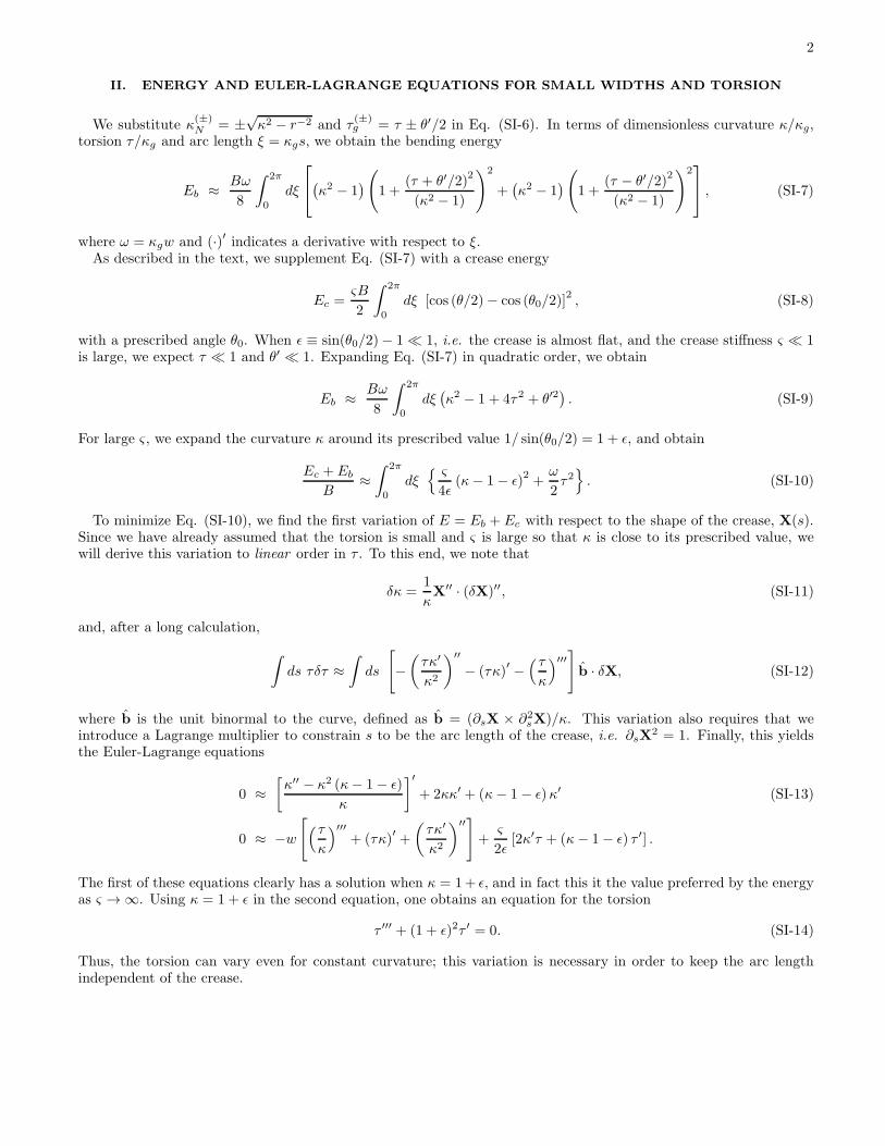
Our numerical model was created by using triangulated meshes to represent the initial, planar setup of the curvedorigami. These meshes are essentially hexagonal grids, designed such that each internal angle π/3. The mesh used inFig. 2b has 7,650 nodes and 14,400 faces, with an effective width of .0994. The mesh shown in Fig. 4b has 15,050nodes and 29,040 faces and an outer radius twice that of its inner radius with six uniformly spaced folds.We endow these triangulated meshes with elastic stretching and bending modes to capture the in-plane and out-

of-plane deformation of thin sheets. The stretching mode simply treats each edge in the mesh as a linear spring,all edges having the same stretching stiffness. Accordingly, the magnitude of the restorative elastic forces applied toeach node in a deformed edge with rest length x0 and stretching stiffness k is given by ks

x0

(x′ − x0) and the energy

contained in a deformed edge is given by ks

2x0

(x′ − x0)2. The x0 term in denominator of the stretching mode ensures

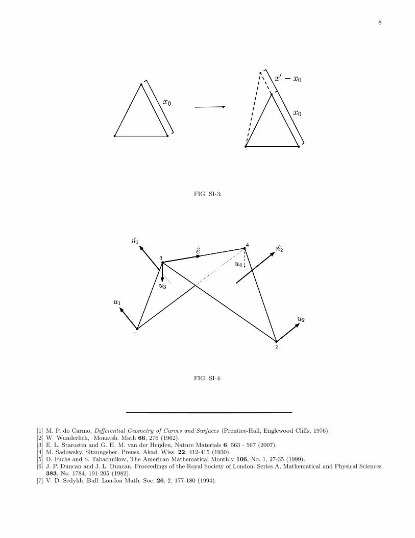
mesh-independence. The bending mode is characterized in terms of four vectors u1, u2, u3 and u4, each of which isapplied to a node in a pair of adjacent triangles. Defining the weighted normal vectors N1 = (x1 − x3) × (x1 − x4)and N2 = (x2 − x4)× (x2 − x3) and the shared edge E = x4 − x3, we may write

u1 = |E| N1

|N1|2(SI-26)

u2 = |E| N2

|N2|2(SI-27)

u3 =(x1 − x4) · E

|E|N1

|N1|2+

(x2 − x4) · E|E|

N2

|N2|2(SI-28)

u4 = − (x1 − x3) · E|E|

N1

|N1|2− (x2 − x2) · E

|E|N2

|N2|2. (SI-29)

The relative magnitudes of these vectors constitute a pure geometric bending mode for a pair of adjacent triangles.For pairs of adjacent triangles that do not straddle the fold line, the force on each vertex is given by

Fi = kb|E|2

|N1|+ |N2|sin(θ/2)ui (SI-30)

where kb is the mesh-independent bending stiffness and sin(θ/2) = ±√

1− n1 · n2/2 is the dihedral angle functionthat makes each ui equivalent to an elastic restorative force. The normalization scales the magnitude of Fi to ensurethat kb is mesh-independent. For pairs of adjacent triangles that do straddle the fold line, the sin(θ/2) term is shiftedby the rest angle θ0 so that the force on each vertex is given by

Fi = kb|E|2

|N1|+ |N2|(sin(θ/2)− sin(θ0/2))ui. (SI-31)

7

This shift makes the rest configuration of a pair of adjacent triangles non-planar and provides the mechanism bywhich we simulate the local plasticity of a fold. Just as a piece of folded paper retains its fold rather than returningto its initial planar state, the adjacent triangles that straddle the curved fold line in the simulated mesh bend out ofthe plane toward their rest angles. The bending energy contained in a pair of adjacent triangles is given by

Eb =kb2

∫ θ

θ0

(sinθ

2− sin

θ02)dθ (SI-32)

where kb is the bending stiffness (*** we need to be precise about the form of the energy here - so how does the pre

factor appear ? ***) and |E|2

|N1|+|N2|, which is quadratic in θ − θ0 for θ ∼ θ0, in agreement with the phenomenological

energy form in the analytical model.We introduce viscous damping so that the simulation eventually comes to rest. Damping forces are computed at

every vertex with different coefficients for each oscillatory mode, bending and stretching. We distinguish betweenthese two modes by projecting the velocities of the vertices in an adjacency onto the bending mode, and the velocitiesof the vertices in an edge onto the stretching mode.The discrete model enables us to construct an equation of motion for each vertex to describe the dynamic behavior

of the mesh. This equation takes the form

x =1

mf(x, x) (SI-33)

where x is the position of the vertex in world coordinates, m is the vertex mass and f(x, x) is the incident force vectorfunction on the vertex in terms of its position vector x and velocity vector x. We discretize this equation and usethe Velocity Verlet numerical integration method to update the positions and velocities of the vertices. At any timet+∆t during the simulation we can approximate the position x(t+∆t) and the velocity x(t+∆t) of a vertex as

x(t+∆t) = x(t) + x(t)∆t+1

2x(t)∆t2 (SI-34)

x(t+∆t) = x(t) +x(t) + x(t+∆t)

2∆t (SI-35)

A single position, velocity and accleration update then follows a simple algorithm.

• Compute x(t+∆t)

• Compute x(t+∆t) using x(t+∆t) for stretching and bending forces and x(t) for damping forces

• Compute x(t+∆t)

Note that this algorithm staggers the effects of damping on the simulation by ∆t.The physical model shown in Fig. 4a was cut from a thin plastic sheet using a laser cutter. The folds were created

by laser cutting fine perforated lines, and the model was then folded by hand. Its geometry matches that of thesimulation shown in Fig. 4b, where we started with a planar annulus and used the natural angle of each curved fold(assumed to be identical) as a single fitting parameter.

8

FIG. SI-3:

FIG. SI-4:

[1] M. P. do Carmo, Differential Geometry of Curves and Surfaces (Prentice-Hall, Englewood Cliffs, 1976).[2] W Wunderlich, Monatsh. Math 66, 276 (1962).[3] E. L. Starostin and G. H. M. van der Heijden, Nature Materials 6, 563 - 567 (2007).[4] M. Sadowsky, Sitzungsber. Preuss. Akad. Wiss. 22, 412-415 (1930).[5] D. Fuchs and S. Tabachnikov, The American Mathematical Monthly 106, No. 1, 27-35 (1999).[6] J. P. Duncan and J. L. Duncan, Proceedings of the Royal Society of London. Series A, Mathematical and Physical Sciences

383, No. 1784, 191-205 (1982).[7] V. D. Sedykh, Bull. London Math. Soc. 26, 2, 177-180 (1994).