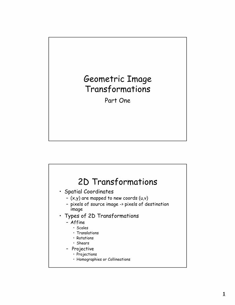
1

Geometric Image Transformations

Part One

2D Transformations• Spatial Coordinates

– (x,y) are mapped to new coords (u,v)– pixels of source image -> pixels of destination

image• Types of 2D Transformations

– Affine• Scales• Translations• Rotations• Shears

– Projective• Projections • Homographies or Collineations

2

Scale and Translation

• Scale– u = s_x * x– v = s_y * y

• Translation– u = x + t_x– v = y + t_y

Rotation and Shears

• Rotation– u = x*cos θ - y * sin θ– v = x*sin θ + y * cos θ

• Shear– u = x + Sh_x * y– v = y + Sh_y * x

3

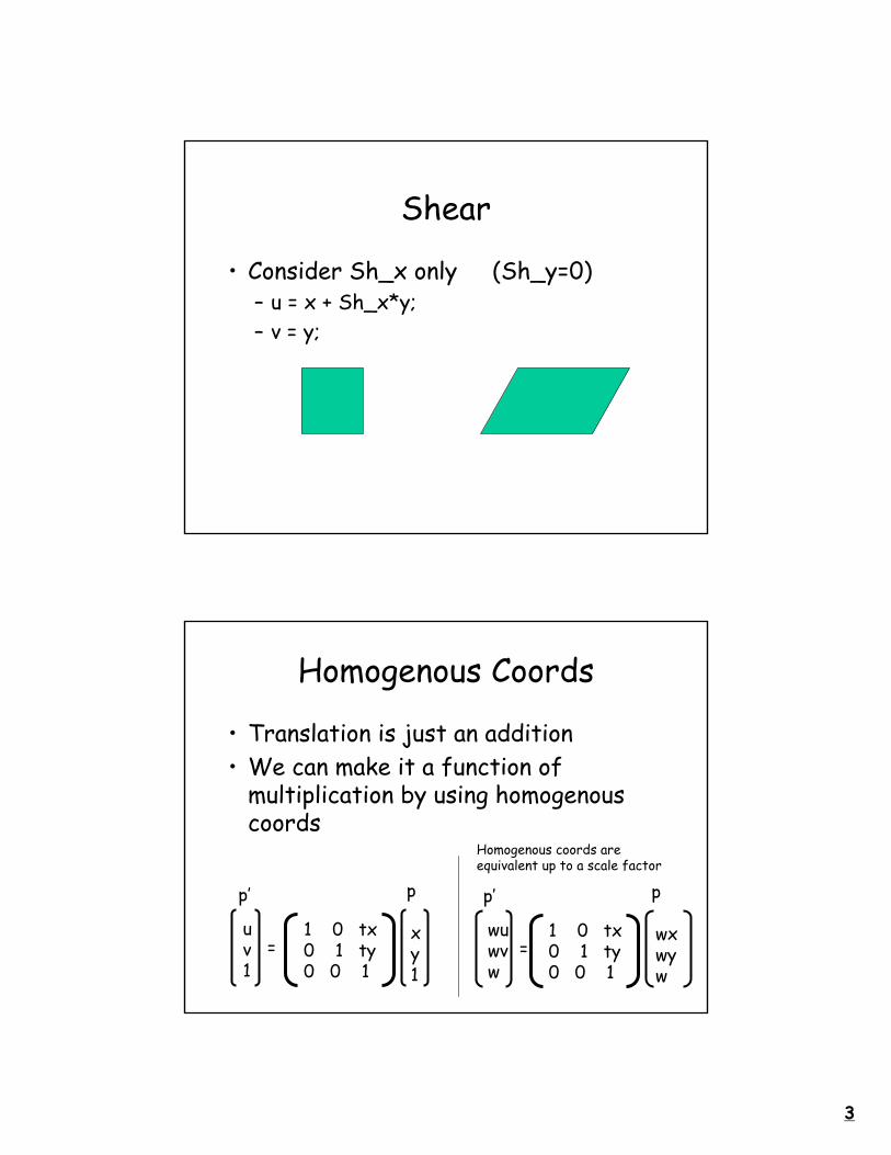
Shear

• Consider Sh_x only (Sh_y=0)– u = x + Sh_x*y;– v = y;

Homogenous Coords

• Translation is just an addition• We can make it a function of

multiplication by using homogenous coords

xy1

p

=uv1

p’

1 0 tx 0 1 ty 0 0 1

wxwyw

p

=wuwvw

p’

1 0 tx 0 1 ty 0 0 1

Homogenous coords are equivalent up to a scale factor

4

Homogenous Coordinates• Transform works on scale (w)

* w

Dividing by the scale “w” puts you in Cartesian coords

w=1

Matrix Notation

a b c d e f 0 0 1

xy1

Affine p

=

uv1

p’

5

Matrix notation of transforms

1 0 tx 0 1 ty 0 0 1

xy1

p

=uv1

p’

Sx 0 0 0 Sy 0 0 0 1

xy1

p

=uv1

p’

cosθ -sinθ 0 sinθ cosθ 0

0 0 1

xy1

p

=uv1

p’

1 Shx 0 Shy 1 00 0 1

xy1

p

=uv1

p’

Translation Scale

Rotation Shear

Concatenation

• You can concatenate several transforms into one matrix

A = R S Sh Trotate scale shear translate

6

Affine Transformations

Affine is a linear mapping plus a translation:– A function f(x) is linear iff

• f(x+y) = f(x) + f(y)• a*f(x) = f(a*x)

– A function T(x) is Affine if there exists• a linear mapping L(x)• and a constant “c”• Such that: T(X) = L(x) + c (for all x)

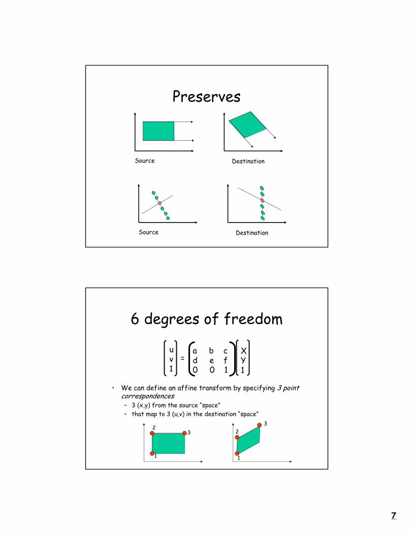
Affine Transforms’ Properties

• Preserves parallel lines• Preserves equispaced points along lines

– equally spaced points on a line in the source space

– will produce equally spaced points on a line in the destination space

– (although the scale may be different)• Preserves incident

– Points of intersection hold

7

Preserves

Source Destination

Source Destination

6 degrees of freedom

XY1

=uv1

a b cd e f 0 0 1

• We can define an affine transform by specifying 3 point correspondences– 3 (x,y) from the source “space”– that map to 3 (u,v) in the destination “space”

1

23

1

23

8

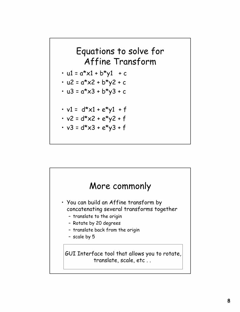
Equations to solve for Affine Transform

• u1 = a*x1 + b*y1 + c• u2 = a*x2 + b*y2 + c• u3 = a*x3 + b*y3 + c

• v1 = d*x1 + e*y1 + f• v2 = d*x2 + e*y2 + f• v3 = d*x3 + e*y3 + f

More commonly

• You can build an Affine transform by concatenating several transforms together– translate to the origin– Rotate by 20 degrees– translate back from the origin– scale by 5

GUI Interface tool that allows you to rotate,translate, scale, etc . .

9

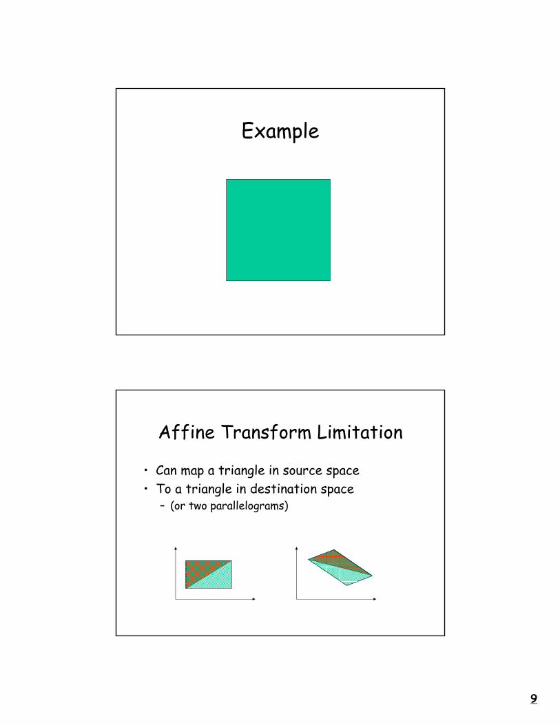
Example

Affine Transform Limitation

• Can map a triangle in source space• To a triangle in destination space

– (or two parallelograms)

10

Affine Transform Limitation

• Can map a triangle in source space• To a triangle in destination space

– (or two parallelograms)

• What about a rectangle to a general quadrilateral?

Projective Transform

• Projective transform can transform general quadrilaterals between source and destination space

• Does not preserve parallel lines, or lengths

• Does not preserve equispaced points

11

Projective transform uses homogenous coords

xy1

=susvs

a b cd e f g h 1

u’ = u/sv’ = v/s

Maps us back to Cartesian space

Projective Transforms• Very common in computer graphics

– Texture mapping a 3D polygon – polygon has been projected onto a plane

Texture map3D perspectiveprojection

3D polygon

2D polygon

12

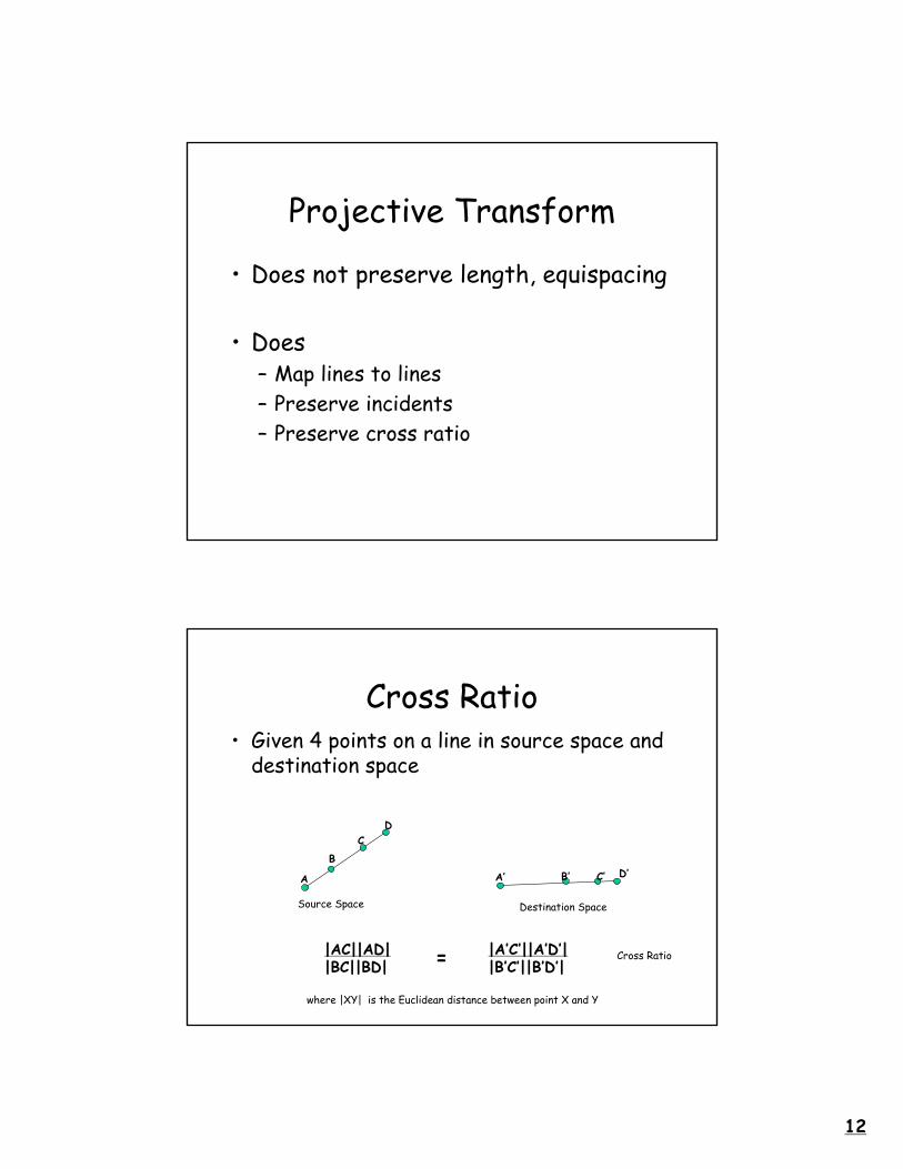
Projective Transform

• Does not preserve length, equispacing

• Does– Map lines to lines– Preserve incidents – Preserve cross ratio

Cross Ratio• Given 4 points on a line in source space and

destination space

A

B

CD

Source Space

A’ B’ C’ D’

Destination Space

|AC||AD||BC||BD|

|A’C’||A’D’||B’C’||B’D’|=

where |XY| is the Euclidean distance between point X and Y

Cross Ratio

13

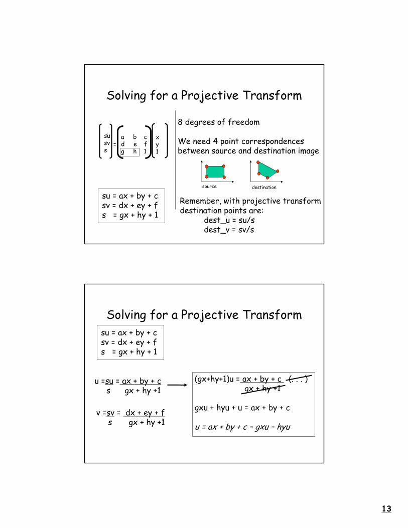
Solving for a Projective Transform

xy1

=susvs

a b cd e f g h 1

8 degrees of freedom

We need 4 point correspondencesbetween source and destination image

su = ax + by + csv = dx + ey + fs = gx + hy + 1

source destination

Remember, with projective transform destination points are:

dest_u = su/sdest_v = sv/s

Solving for a Projective Transformsu = ax + by + csv = dx + ey + fs = gx + hy + 1

u =su = ax + by + cs gx + hy +1

v =sv = dx + ey + fs gx + hy +1

(gx+hy+1)u = ax + by + c (. . . )gx + hy +1

gxu + hyu + u = ax + by + c

u = ax + by + c – gxu – hyu

14

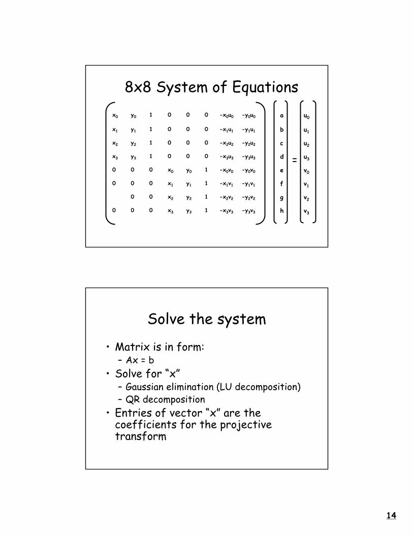
8x8 System of Equations

v3h-y3v3-x3v31y3x3000

v2g-y2v2-x2v21y2x200

v1f-y1v1-x1v11y1x1000

u3d-y3u3-x3u30001y3x3

v0e-y0v0-x0v01y0x0000

u2c-y2u2-x2u20001y2x2

u1b-y1u1-x1u10001y1x1

u0a-y0u0-x0u00001y0x0

=

Solve the system

• Matrix is in form:– Ax = b

• Solve for “x”– Gaussian elimination (LU decomposition)– QR decomposition

• Entries of vector “x” are the coefficients for the projective transform

15

Properties of Transforms

XXnon-uniform scale

Xcombination (w/ projection)

Xprojection

XXshear

XXXuniform scale

XXXXrotation

XXXXtranslation

Transformation

projectiveaffinesimilarityeuclidean

Properties of Transforms

XXXparallelism

XXXXcross ratio

XXXXincident

XXratio of lengths

XXangle

Xlength

Invariant

projectiveaffinesimilarityeuclidean

16

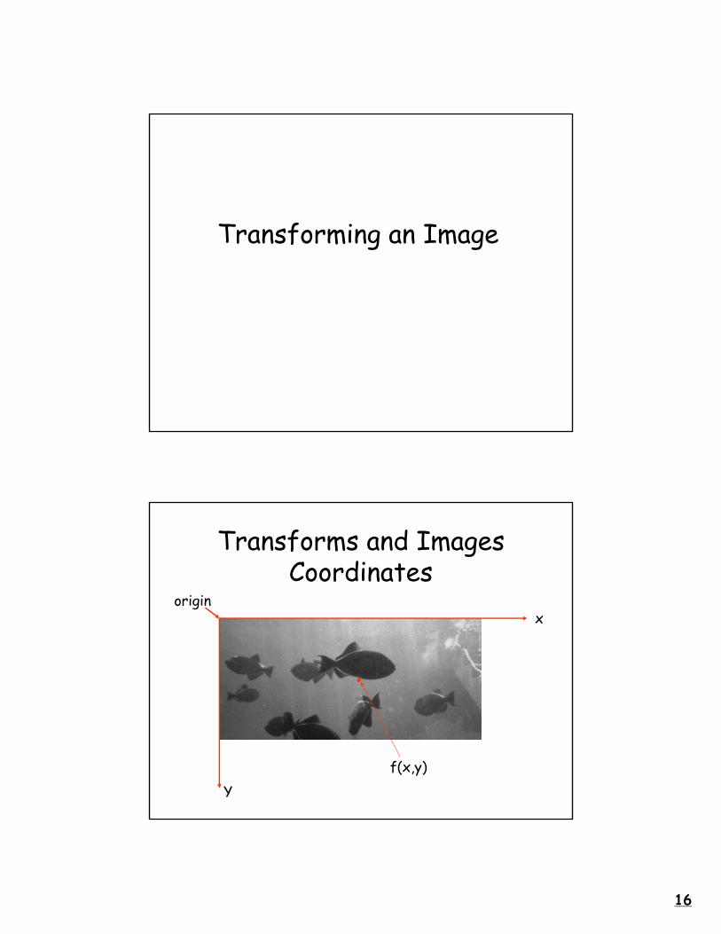
Transforming an Image

Transforms and Images Coordinates

Y

xorigin

f(x,y)

17

Image Coords vs. Cartesian Coords

• Image Coords are generally defined by raster alignment– Y [0,Height], X [0,Width]

• Affine, projective transforms are converted into Cartesian coords

Transforms and Images Coordinates

Y

xorigin

f(x,y)

(-y value)

18

Cartesian space to image space

• From Cartesian space to Image Space– find (x_min, xmax)– find (y_min, ymax)

– new size dimensions• w = x_max – x_min• h = y_max – y_min• create newImage size (w, h)

– Translate transformed points, such that:• T * (x,y) = (u,v)• newImage( u + abs(x_min), v + abs(y_min) = I(x,y)

Converting to an Image

Y

xorigin

New Image Dimensions

19

The transformed image

Y

xorigin New Image Dimensions

Creating the “new” image

• Forward Mapping • Inverse Mapping• Sampling

20

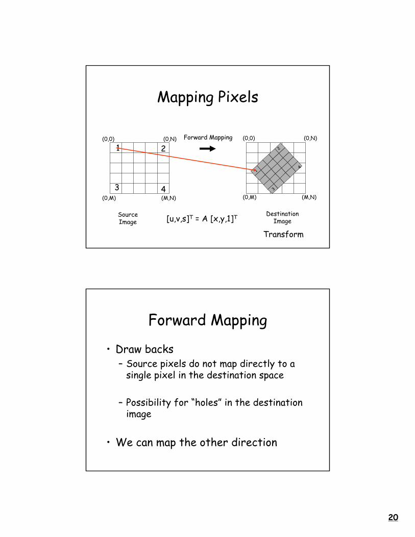
Mapping Pixels

(0,0) (0,N)

(0,M) (M,N)

Transform

(0,0) (0,N)

(0,M) (M,N)

1 2

3 4

1

2

3

4

DestinationImage

SourceImage

Forward Mapping

[u,v,s]T = A [x,y,1]T

Forward Mapping

• Draw backs– Source pixels do not map directly to a

single pixel in the destination space

– Possibility for “holes” in the destination image

• We can map the other direction

21

black

Reverse Mapping

(0,0) (0,N)

(0,M) (M,N)

1 2

3 4

1

2

3

4

Reverse Mapping

1

23

4

1 2

3 4

[x,y,s]T = A-1[u,v,1]T

“Inverse” Mapping

• Advantages– We assign an “intensity” to each pixel in

the destination (no holes)– Affine/projective transforms have

inverses (not a problem)• just reverse direction of the point

correspondences• We still don’t have pixel to pixel

mapping

22

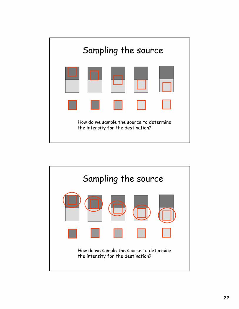
Sampling the source

How do we sample the source to determinethe intensity for the destination?

How do we sample the source to determinethe intensity for the destination?

Sampling the source

23

MappingSource

2 x 2 pixels

Option 1 : Pick the pixel nearest to our center.

MappingSource

2 x 2 pixels

Option 1 : Pick the pixel nearest to our center.

Small change results in big difference

24

Try different samplingSource

2 x 2 pixelsWhat if we assign an intensityto each vertex and then average?

1 2

3 4

1 2 3 4

Pick the intensity which the vertexlies.

New Sample =

Sampling ExampleSource

2 x 2 pixelsMove the destination slightly.

1 2

3 4

1 2 3 4

Pick the intensity which the vertexlies.

New Sample =

25

No DifferenceSource

2 x 2 pixels

1 2

3 4

Source2 x 2 pixels

1

2

3

4

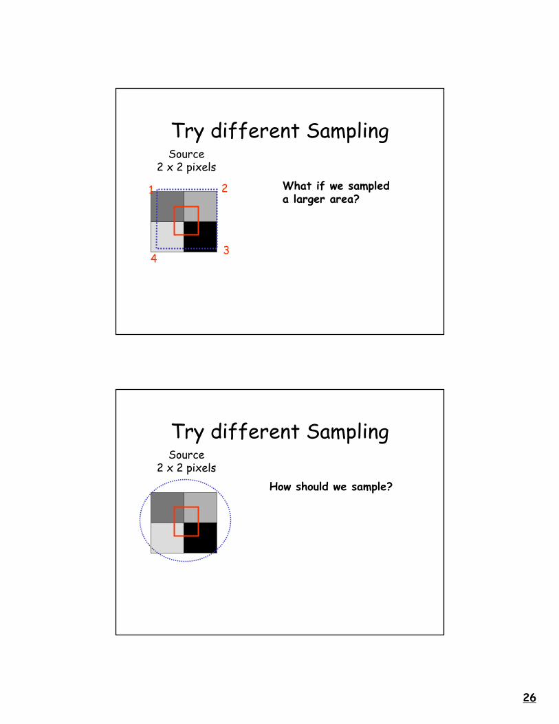
Try different SamplingSource

2 x 2 pixels

1

23

4

What if we had more samples?

26

Try different SamplingSource

2 x 2 pixels

1 2

34

What if we sampleda larger area?

Try different SamplingSource

2 x 2 pixelsHow should we sample?

27

Common Sampling Approaches• Nearest Neighbor

– 1 Sample– Take closest pixel value

• Bi-linear Interpolation– 2x2 (4) Samples– Interpolate from these samples– Slower

• Bi-Cubic– 4x4 (8) samples– Construct a new sample using a non-linear “interpolation”– Slower

Common Sampling Approaches

Bi-Cubic

Bi-linear Interpolation

Nearest Neighbor

28

Common Sampling Approaches

Bi-Cubic

Bi-linear Interpolation

Nearest Neighbor

•What do these approaches mean?

•How can evaluate what they are doing?

Sampling and Signal Processing• Proper sampling is a classic “reconstruction problem”• Given a continuous signal f(x)• How do you take discrete samples such that you can properly

reconstruct the signal f(x) from the samples?

f(x)

x