Geometric Continuity: by Anthony D. DeRose
148
... Geometric Continuity: A Parametrization Independent Measure of Continuity for Computer Aided Geometric Design by Anthony D. DeRose In Partial Fulfillment of the Requirements for the Degree of Doctor of Philosophy . m Computer Science University of California Berkeley, California August, 1985
Transcript of Geometric Continuity: by Anthony D. DeRose

...
Geometric Continuity:
A Parametrization Independent
Measure of Continuity for
Computer Aided Geometric Design
by
Anthony D. DeRose
In Partial Fulfillment of the Requirements
for the Degree of
Doctor of Philosophy . m
Computer Science
University of California
Berkeley, California
August, 1985

Report Documentation Page Form ApprovedOMB No. 0704-0188
Public reporting burden for the collection of information is estimated to average 1 hour per response, including the time for reviewing instructions, searching existing data sources, gathering andmaintaining the data needed, and completing and reviewing the collection of information. Send comments regarding this burden estimate or any other aspect of this collection of information,including suggestions for reducing this burden, to Washington Headquarters Services, Directorate for Information Operations and Reports, 1215 Jefferson Davis Highway, Suite 1204, ArlingtonVA 22202-4302. Respondents should be aware that notwithstanding any other provision of law, no person shall be subject to a penalty for failing to comply with a collection of information if itdoes not display a currently valid OMB control number.
1. REPORT DATE AUG 1985 2. REPORT TYPE
3. DATES COVERED 00-00-1985 to 00-00-1985
4. TITLE AND SUBTITLE Geometric Continuity: A Parametrization Independent Measure ofContinuity for Computer Aided Geometric Design
5a. CONTRACT NUMBER
5b. GRANT NUMBER
5c. PROGRAM ELEMENT NUMBER
6. AUTHOR(S) 5d. PROJECT NUMBER
5e. TASK NUMBER
5f. WORK UNIT NUMBER
7. PERFORMING ORGANIZATION NAME(S) AND ADDRESS(ES) University of California at Berkeley,Department of ElectricalEngineering and Computer Sciences,Berkeley,CA,94720
8. PERFORMING ORGANIZATIONREPORT NUMBER
9. SPONSORING/MONITORING AGENCY NAME(S) AND ADDRESS(ES) 10. SPONSOR/MONITOR’S ACRONYM(S)
11. SPONSOR/MONITOR’S REPORT NUMBER(S)
12. DISTRIBUTION/AVAILABILITY STATEMENT Approved for public release; distribution unlimited
13. SUPPLEMENTARY NOTES
14. ABSTRACT Parametric spline curves and surfaces are typically constructed so that some number of derivatives matchwhere the curve segments or surface patches abut. If derivatives up to order n are continuous, thesegments or patches are said to meet with C^ n, or nth order parametric continuity. It has been shownpreviously that parametric continuity is sufficient, but not necessary, for geometric smoothness. Thegeometric measures of unit tangent and curvature vectors for curves (objects of parametric dimensionone), and tangent plane and Dupin indicatrix for surfaces (objects of parametric dimension two), have beenused to define first and second order geometric continuity. These measures are intrinsic in that they areindependent of the parametrizations used to describe the curve or surface. In this work, the notion ofgeometric continuity as a parametrization independent measure is extended for arbitrary order n (G^n),and for objects of arbitrary parametric dimension p. Two equivalent characterizations of geometriccontinuity are developed: one based on the notion of reparametrization, and one based on the theory ofdifferentiable manifolds. From the basic definitions, a set of necessary and sufficient constraint equations isdeveloped. The constraints (known as the Beta constraints) result from a direct application of theunivariate chain rule for curves and the bivariate chain rule for surfaces. In the spline construction processthe Beta constraints provide for the introduction of freely selectable quantities known as shape parameters.For polynomial splines, the use of the Beta constraints allows greater design flexibility through the shapeparameters without raising the polynomial degree. The approach taken is important for several reasons.First, it generalizes geometric continuity to arbitrary order for both curves and surfaces. Second, it showsthe fundamental connection between geometric continuity of curves and that of surfaces. Third, due to thechain rule derivation, constraints of any order can be determined more easily than using derivations basedexclusively on geometric measures. Finally, a firm connection is established between the theory ofdifferentiable manifolds and the use of parametric splines in computer aided geometric design.
15. SUBJECT TERMS

16. SECURITY CLASSIFICATION OF: 17. LIMITATION OF ABSTRACT Same as
Report (SAR)
18. NUMBEROF PAGES
146
19a. NAME OFRESPONSIBLE PERSON
a. REPORT unclassified
b. ABSTRACT unclassified
c. THIS PAGE unclassified
Standard Form 298 (Rev. 8-98) Prescribed by ANSI Std Z39-18

GEOMETRIC CONTINUITY:
A PARAMETRIZATION INDEPENDENT
MEASURE OF CONTINUITY FOR
COMPUTER AIDED GEOMETRIC DESIGN
Copyright © 1985
Anthony D. DeRose

FOR MY MOTHER
...


Acknowledgments
I would like to thank my thesis advisor, Brian Barsky, for providing a sometimes
hectic, but always exciting, research environment. Through him, many opportu
nities have been presented to me that would have otherwise been impossible. I
would also like to thank Beresford Parlett for serving as the ever-present "outside
member", and for enduring several afternoons of obscure questions.
Special thanks is in order to Ron Goldman, the third member of my commit
tee. From the beginning, Ron has treated this research with astounding care and
enthusiasm, often providing deep, insightful comments. It must be rare for a grad
uate student to find a committee member willing to spend the kind of time and
effort that Ron has devoted to this dissertation, and I am indeed grateful for his
participation.
The arduous progression from first year status, through prelims, quais, and
finally the dissertation, has actually been quite pleasurable, due in large part to
an eclectic group of friends, including: Gregg Foster, Mark Hill, Susan Eggers,
Steve Upstill, Prabhakar Ragde, John Gross, Ken Fishkin, Lindy Foster, and my
roommates for the last two years, Garth Gibson and Pounce.
I'd also like to thank Mom, Dad and my sister Dianne, for believing me when
I said I'd someday finish my P-H-D and get a real J-0-B. Finally, there's Cindy
Babuska- the gal that has had to put up with me through this ordeal. Lord knows
it hasn't been easy for her, but she didn't even complain when we had to cancel our
Mexican vacation.
This work was supported in part by the Defense Advanced Research Projects
Agency under contract number N00039-82-C-0235, the National Science Foundation
under grant number ECS-8204381, the State of California under a Microelectron
ics Innovation and Computer Research Opportunities grant, and a Shell Doctoral
Fellowship.


Contents
1. Introduction . . • . . . . •
1.1. Overview . . . . . . .
1.2. Notation and Conventions
2. An Intuitive Approach
2.1. Introduction . . .
2.2. Previous Work ..
2.3. Reparametrization and the Chain Rule
2.4. Geometric Continuity for Curves . . .
2.5. Continuity of Surfaces . . . . . . . .
2.5.1. Parametric Continuity for Surface Patches
2.5.2. Reparametrization of Surface Patches
2.5.3. Geometric Continuity for Surface Patches
2.5.3.1. Equivalence with Previous Measures
2.6. Summary . . . . . . . .
3. Spline Curves
3.1. Background
3.1.1. Bezier Curves .
3.1.2. B-spline Curves
3.2. Placement of Bezier Vertices
3.3. Beta-spline Curves . . . .
3.4. Geometrically Continuous Catmull-Rom Splines
3.5. Summary . . . . . . . . .
4. Tensor Product Surfaces
4.1. Introduction . . . .
4.2. Geometric Continuity of Tensor Product Surfaces
4.3. Summary . . . . . . . . . .
5. Triangular Spline Surfaces
Page
1
3
5
7
7
11
. 14
15 20
23
28 . 31
. 35
. 38
• • 40
. 40
. 42
. 43
. 44
. 46
. 48
. 49
• • • . 51
51 52
52
. • •. 54

5.1. Introduction . . . . . .
5.2. Notation . . . . . . . .
5.3. Triangular Bezier Surfaces
5.4. Triangular B-splines . . .
ii
. 54
. 55
0 55
0 59
5.5. Triangular Beta-spline Surfaces . 60
5.5.1. Derivation of the Triangular Cubic Beta-spline Basis Patches . 61
5.5.2. Evaluation Algorithm . . . .
5.6. Summary
6. Foundations of Geometric Continuity
6.1. Introduction . . . . . . . . . . .
6.2. Some Concepts from Elementary Topology
6.3. A Brief Review of Multivariate Calculus
6.4. Elementary Manifold Theory
6.4.1. Orientable Manifolds .
6.4.2. Maps on Manifolds
6.5. Abstract Splines . . . .
6.6. Parametric Splines
6.7. Weak Geometric Continuity, war Splines
6.8. ar Splines . . . . . . . . . . . . . .
6.9. Beta Constraints: Application of the Theory
6.9.1. Transition Graphs
6.10. Equivalence Theorems
6.11. Summary . . . . .
7. Conclusions
References . • . .. .
. 70
. 73
• • 16
. 76
. 79
0 79
' 82
. 86
. 87
. 91
. 95
101 106
112
119
120
124
127
130

1
Geometric Continuity:
A Parametrization Independent Measure
of Continuity for Computer Aided Geometric Design
Anthony D. DeRose
ABSTRACT
Parametric spline curves and surfaces are typically constructed so that some number
of derivatives match where the curve segments or surface patches abut. If derivatives
up to order n are continuous, the segments or patches are said to meet with en, or nth order parametric continuity. It h~ been shown previously that parametric
continuity is sufficient, but not necessary, for geometric smoothness.
The geometric measures of unit tangent and curvature vectors for curves ( ob
jects of parametric dimension one), and tangent plane and Dupin indicatrix for
surfaces (objects of parametric dimension two), have been used to define first and
second order geometric continuity. These measures are intrinsic in that they are
independent of the parametrizations used to describe the curve or surface. In this
work, the notion of geometric continuity as a parametrization independent mea
sure is extended for arbitrary order n (an), and for objects of arbitrary parametric
dimension p. Two equivalent characterizations of geometric continuity are devel
oped: one based on the notion of reparametrization, and one based on the theory
of differentiable manifolds.
From the basic definitions, a set of necessary and sufficient constraint equa
tions is developed. The constraints (known as the Beta constraints) result from a
direct application of the univariate chain rule for curves and the bivariate chain
rule for surfaces. In the spline construction process the Beta constraints provide
for the introduction of freely selectable quantities known as shape parameters. For
polynomial splines, the use of the Beta constraints allows greater design flexibility
through the shape parameters without raising the polynomial degree.
The approach taken is important for several reasons. First, it generalizes geo
metric continuity to arbitrary order for both curves and surfaces. Second, it shows
the fundamental connection between geometric continuity of curves and that of

2
surfaces. Third, due to the chain rule derivation, constraints of any order can be
determined more easily than using derivations based exclusively on geometric mea~
sures. Finally, a firm connection is established between the theory of differentiable
manifolds and the use of parametric splines in computer aided geometric design.

1
1
Introduction
In the early days of computer aided geometric design (CAGD) a.nd computer
graphics, it was common to model objects with linear segments or pla.na.r polygonal
facets. However, polygonal modeling is not well suited to the modeling of smoothly
varying objects such as the outline of a. character in a. typography system, the
surface of a. ship hull, or the skin of a.n airplane. To define objects such as these,
higher order curve a.nd surface models known parametric splines have become
popular. Parametric splines a.re piecewise functions, so care must be taken to
"stitch" the curve segments or surface patches together in a. "smooth" fashion. It
is the fundamental notion of smoothness that this work addresses.
The usual measure of smoothness, known as parametric continuity, requires
the piecing together of curves a.nd surfaces so that a. given number of parametric
derivatives match a.t the boundaries between curve segments or surface patches.
The order of continuity (the number of derivatives that a.re required to match)
is determined by the particular application. Although this generally results in
splines that "look" smooth, it is shown in Chapter 2 that parametric continuity
ca.n be overly restrictive since it depends upon details of the pa.ra.metriza.tions that
a.re irrelevant for many CAGD applications.
To remedy this situation, we define a. measure of continuity, known as
geometric continuity, that is insensitive to changes in these irrelevant details. In
other words, geometric continuity is a. parametrization independent measure of
continuity. The definition of geometric continuity (to be given in Chapter 2) is
concise a.nd conceptually simple, but it is a. definition based on the existence of
certain equivalent parametrizations. As such, it is a. definition that does not lend
itself to practical use.

1. INTRODUCTION 2
To achieve a practical definition of geometric continuity, a set of constraint
equations, known as Beta constraints, is derived from the basic definition. These
constraints are necessary and sufficient conditions for geometric continuity of the
spline. It is shown that the Beta constraints result from a direct application of the
chain rule for differentiation: the univariate chain rule for curves, the bivariate
chain rule for surfaces, the trivariate chain rule for volumes, and so on for objects
of higher parametric dimension.
Geometric continuity is not only of theoretic interest, but also has practical
uses. Due to its parametrization independent nature, a large number of splines
that are not parametrically smooth are geometrically smooth. For instance, the
class of piecewise geometrically continuous polynomial splines of degree d strictly
includes the class of piecewise parametrically continuous splines of degree d (see
Figure 1.1).
The generality of geometric continuity is reflected in the Beta constraints
through the introduction of variable quantities called shape parameters. The shape
parameters are degrees of freedom that are not available when using parametric
continuity. The shape parameters can be made available to a designer in a CAG D
environment. If the spline technique is based on the Beta constraints rather
than the parametric continuity constraints, the shape parameters can be used
to alter the shape of the curve or surface. Experience has shown that shape
parameter modification can be a very effective method of shape control [3,4,5].
Moreover, shape parameter modification can be performed independent of the
other controls the designer has over shape. Specific examples of this process are
given in Chapters 3, 41 and 5.
Previous definitions of parametrization independent measures of continuity
were either based on certain fundamental geometric measures, to be discussed
in Section 2.2, or, like ours, were based on the existence of equivalent parame
trizations. Each of these approaches have had their problems. For instance, the
derivation of the Beta constraints from geometric measures is often cumbersome
and error prone. Moreover, it seems difficult to define continuity for order higher
than two, and if such definitions were to be stated, it is likely that the algebra re
quired to derive the Beta constraints would be prohibitively complex. On the other
hand, previous work on existence definitions have failed to derive general Beta con
straints for third order and higher. Finally, all previous work has treated curves
and surfaces completely separately. Thus, all practical work on parametrization
independent measures has been restricted to first and second order continuity for

1. INTRODUCTION 3
geometrically continuous
parametrically continuous
Figure 1.1. The class of geometrically continuous polynomial splines of a given
degree is a strict generalization of the class of parametrically continuous splines of
the same degree. The shape parameters are used to explore the larger design space
provided by geometric continuity.
curves and surfaces (see Figure 1.2).
Although first and second order continuity for curves and surfaces is sufficient
for many applications, there are situations where higher order continuity or higher
parametric dimension is needed. For instance, third order continuous curves
and surfaces find application in ship hull design [48], and objects of parametric
dimension three and four naturally arise in computer graphics animation [25].
Thus, it is desirable to define and describe geometric continuity for higher order
and higher parametric dimension.
This work characterizes geometric continuity for arbitrary order, and for
arbitrary parametric dimension. Perhaps more importantly, the extension to
higher order continuity and higher parametric dimension is done in a unified way,
and it is shown that the Beta constraints can be easily derived. The extension is
unified in the sense that geometric continuity for curves, surfaces, volumes, etc.,
are all developed as manifestations of the same underlying theory (see Figure 1.2).
The primary purpose of this work is to characterize the nature of geometric
continuity by examining the smoothness properties of geometrically continuous
splines, providing many alternate definitions of geometric continuity, and proving
that the Beta constraints may be easily derived. However, it is not the purpose
of this work to completely characterize the use of geometric continuity in CAGD.
Rather, we present several examples of its use, leaving a comprehensive investiga
tion of the uses of geometric continuity as a topic of future research.

1. INTRODUCTION 4
Order ---. 1 2 3
1 0 0 . . .
0 0 . . . . . . . . .
Figure 1.2. The figure above is a tabular depiction of the "problem space 11
of geometric continuity. The order of continuity increases to the right, and the
parametric dimension increases downward. The first row therefore corresponds
to geometric continuity for curves, the second row to surfaces, the third row to
volumes, and so on. Circles denote those instances of geometric continuity for
which basic definitions have previously been given, and Beta constraints derived.
This work fills out all entries of the doubly infinite table in a unified way.
1.1. Overview
The presentation is logically divided into three parts:
Part I, consisting of Chapter 2, presents an intuitive approach to geometric
continuity for curves and surfaces. Virtually all the central results of the theory
are developed using plausibility arguments rather than formal proofs. The
development is based on the notion of reparametrization in conjunction with the
chain rule. The relationship between this work and previous work is also discussed.
Part II, consisting of Chapters 3, 4, and 5, discusses some applications
of the theory of geometric continuity. In Chapter 3, the use of geometric
continuity and the Beta constraints is discussed for parametric curves. Chapter 4
shows that a surface constructed by forming a tensor product of geometrically
continuous curves, produces a geometrically continuous surface. In Chapter 5,
geometrically continuous triangular surface techniques are explored. These include
the placement of control vertices for Blzier triangles, and the construction of a new
triangular surface technique called the triangular cubic Beta-spline. The triangular
cubic Beta-spline is a surface technique that possesses one shape parameter and
guarantees tangent plane continuity. An evaluation algorithm for triangular cubic

1. INTRODUCTION 5
Beta-spline surfaces based on recursive subdivision is also developed.
Part III, consisting of Chapter 6, presents a formal development of the
concepts and results contained in Part I. This is done by casting the spline
construction problem into the language of differentiable manifolds. It is shown
that splines can be viewed as differentiable deformations of domain manifolds.
This view of spline construction is particularly convenient because it allows
parametrization indepe:1dent statements to be made in a natural way. The
manifold approach is also important because it firmly establishes the connection
between splines in CAGD and differentiable manifold theory, thereby allowing the
full power of manifold theory to be brought to bear on problems in CAGD. It is
believed that geometric continuity is but one instance of the usefulness of manifold
theory in CAGD.
It is suggested that Parts I and II be read by those seeking a high-level under
standing of geometric continuity and geometrically continuous spline techniques.
Readers interested in a rigorous, in-depth development of the theory of geometric
continuity are encouraged to read Part III. Part III may also be of interest to those
wishing to use manifold theory in CAGD. However, a warning is in order: Part III
assumes a good deal of mathematical sophistication. This method of presentation
was chosen so that the rather obscure (albeit powerful) formal development of Part
III does not hide the essentially simple ideas and results of geometric continuity
presented in Parts I and II.
1.2. Notation and Conventions
• The symbols Z, Z+, 1R, and 1R+ will be used to denote the set of integers,
non-negative integers, reals, and non-negative reals, respectively.
• We use a diacritical vector to denote integer tuples such as k = ( k1 , k2 , ••• , kn).
Unless otherwise stated, the components are assumed to be chosen from Z+.
The norm of k, denoted lkl, is defined to be the sum of the components of k.
• Following the notation of Farin [30], it is convenient to denote by h a tuple
whose components are all zero, except for the sth component, which is one.
• The body of definitions, theorems, lemmas, remarks, and examples are set in
slanted type to clearly distinguish them from the surrounding text.
• In Parts I and II, we set scalars and scalar-valued functions in Italics; vectors,
points, and point-valued functions are set in bold face type. This convention
does not apply to Part III however, since no distinction is made between

1. INTRODUCTION 6
scalars, and points (or vectors). That is, a scalar is simply a point in !Rm,
with m = 1.
• Given a function such as f(x), we denote the ith derivative by f(i) (x),
• Given a function such as g(x, y), we use the notation g(i,i)(x, y) to denote the
ith partial derivative with respect to x and the jtn partial with respect to y.
That is, aHig
g(i,j)(:r;, y) = . . . a•xa'y
• For brevity, and when no ambiguity can arise, the point of evaluation (x, y)
is left off expressions such as g(l,O)(x, y) yielding simply g(l,o).
• Wherever possible, we use the convention that piecewise functions are denoted
by upper case letters; the corresponding lower case letter with appropriate
subscripts will be used to denote the constituent functions.

2
An Intuitive Approach
This chapter takes an intuitive approach to the development of geometric
continuity. The word "intuitive" is meant to suggest that plausibility
arguments rather than formal proofs will be used. We begin with some
background material, then show that parametric continuity can be overly
restrictive for many applications in CAGD. Next we examine previous
work dealing with parametrization independent measures of continuity.
We then develop geometric continuity of arbitrary order for curves,
including a derivation of the univariate Beta constraints. Finally, the
notion of geomet·ric continuity is extended to surfaces.
2.1. Introduction
7
Computer-based modeling requires an unambiguous definition of objects in a
form that can be efficiently stored and manipulated. Perhaps the simplest method
of definition is polygonal modeling. In a polygonal model, objects are described
using points in space, called vertices. The vertices are then logically connected
with edges; a closed loop of vertices and edges defines a face, and a collection of
faces defines an object. Despite their simplicity, polygonal models are not well
suited to the modeling of objects composed of curved boundaries and smoothly
varying surfaces.
There are many ways to model curves and surfaces in a computer amenable
way. Quadric surfaces, implicit equations, solutions of differential equations, and
parametric functions are but a few of the possibilities. Due to their relative
simplicity and flexibility, we will concentrate on curve and surface definitions based

2. AN INTUITIVE APPROACH 8
on parametric functions.
Curves can be defined or generated by one variable parametric functions,
also known a.s univariate parametrizations. A univariate parametrization is a
point-valued function such a.s 1( u) = ( x( u), y( u)), where the domain parameter
u is allowed to range over some interval [u0 , ui]. For a. given value of u, the
function 1( u) can be thought of a.s locating a. particle in Euclidean two-space.
As u is increased over the interval, the particle traverses a. path defined by 1,
tracing out a. curve in the process (see Figure 2.1). If [u0 , ut] is thought of a.s a.n
oriented line segment, then 1 can be thought of a.s a. deformation producing a.n
oriented curve. One advantage of the parametric representation is that a. curve in
Euclidean space of arbitrary dimension d can be described by a. parametrization
1(u) = (x1 (u),x2 (u), ... ,xd(u)) .
...
1
Figure 2.1. The univariate parametrization 1 generates an oriented curve by
deformation of the oriented line segment [ u0 , u1].
A surface patch in three-space can be defined by a. bivariate function such a.s
G(u,v) = (X(u,u),Y(u,u),Z(u,u)),
where u and v are allowed to range over some region DG of the uv plane (see
Figure 2.2). Surface patches in higher dimensions can be described by adding
additional component functions. Loosely speaking, a. surface is a. collection of
surface patches.
For a. curve generated by 1(u), the first derivative vector 1(1>(u) represents the
velocity of the particle. The velocity is a. vector quantity and, a.s such, contains
information about orientation and rate, or speed. The second derivative vector

....
2. AN INTUITIVE APPROACH 9
G
Figure 2.2. The bivariate parametrization G deforms the oriented domain DG
to generate an oriented surface patch.
1(2 ) represents the acceleration of the particle, so it too contains information about
the rate (specifically, the change of rate). Thus, a parametrization contains infor
mation about the geometry (the shape or image of the curve), the orientation, and
the rate. Figure 2.3 shows the curves generated by three different parametriza
tions. The shape of the curves is identical; they differ only in orientation and rate.
Curves (a) and (b) have the same orientation at each point, but the rates differ.
The curve labeled (c) differs from (a) and (b) in orientation and rate. If a curve
is defined to be simply the geometry of a parametrization, one would conclude
that figures (a), (b), and (c) represent equivalent curves. We will refer to this
as the G model of a curve. Another possibility is to consider the geometry and
orientation, which we will call the GO model. Using the GO model, one would say
that (a) and (b) are equivalent, but (c) is different. The last possibility we will
consider is the GOR model, where geometry, orientation, and rate are all relevant
to the definition of a curve. Using this model, no pair of the curves in Figure 2.3
is equivalent.
Parametric spline curves are typically constructed by stitching together
univariate parametric functions, requiring that some number of derivatives match
at each joint (the points where the curve segments meet). If n derivatives agree at
a given joint, the parametrizations there are said to meet with nth order parametric
continuity ( C" continuity for short).
We maintain that the choice of a particular model for a curve, and hence
the choice of how the curve segments are stitched together, should be application
dependent. For instance, if a spline is being used to define the motion of an object
in an animation system, the GO R model is most appropriate since orientation and

2. AN INTUITIVE APPROACH 10
(a) (b) (c)
Figure 2.3. Each of the curves above has the same image; they only differ in
orientation and rate. Orientation is indicated by arrowheads and rate is indicated
by vectors tangent to the curves.
rate are important. In this type of application, parametric continuity is required
to maintain the smoothness of the rate. In other words, parametric continuity will
ensure that the object will move smoothly.
However, in CAGD the rate of a parametrization is often unimportant.
Consider for example the use of splines to describe numerically-controlled cutters.
It may be necessary to specify uniquely the direction of the cutter at each point
on the path, but the speed of the cutter may depend upon the hardness of the
material being cut. For this type of application, the GO model is most suitable,
but parametric continuity is overly restrictive since it places emphasis on irrelevant
rate information. The structure provided by orientation can also be useful for
surfaces. An oriented surface has a consistently defined normal vector that allows
the notions of "top" and "bottom", or "inside" and "outside" to be uniquely
defined. This information can often be useful in practice. For instance, a renderer
in a computer graphics environment can use orientation information to shade the
top of the surface differently from the bottom.
Many other applications in CAGD require only the G model. For instance, if
a spline curve is being used to describe ·the outline of a character in a typography
system, only the shape of the outline is relevant. However, it is difficult to develop
a useful formalism based only on the geometry of a curve or surface. The difficulty
arises because of the global nature of the G model. That is, the geometry of a curve
or surface cannot be completely characterized by examining local neighborhoods -

2. AN INTillTIVE APPROACH 11
geometry is a. global property. In fields such as topology a.nd differential geometry
it is well known tha.t global statements a.re difficult a.nd few. Orientation, however,
is a. local property, so the GO model is a.lso local. The structure provided by
orientation allows a. local theory of continuity to be developed. Hence, we adopt
the GO model a.nd develop a.n appropriate measure of continuity - one based only
on geometry a.nd orientation. We refer to this measure as geometric continuity,
a. term first introduced by Barsky & Beatty [6]. Although it is common to use
parametric polynomial pa.ra.metriza.tions, the development of geometric continuity
we present is valid for a.n extremely large cla.ss of pa.ra.metriza.tions to be identified
subsequently.
2.2. Previous Work
Ma.ny authors ha.ve independently defined parametrization independent mea
sures of continuity for first a.nd second order (which we denote by G1 a.nd G2 ,
respectively) for curves a.ndjor surfaces using geometric means. For curves,
Fowler & Wilson [34], Sabin [52], Manning [47], Fa.ux & Pratt [32], a.nd Barsky [3J
ea.ch defined first order continuity by requiring tha.t the unit tangent vectors agree
a.t the joints. For a. curve generated by I( u), the unit tangent vector a.t the point
I(u), denoted t(u), points in the sa.me direction as I( 1)(u), but is required to be of
unit length (see Figure 2.4). Thus, t(u) is defined by
,... I( 1)(u) t(u) = II(l)(u)l" (2.1)
The unit tangent is a. parametrization independent characterization of the curve
to first order. The requirement of matching unit tangent vectors is therefore
a. first order parametrization independent measure of continuity for curves (see
Figure 2.4).
A second order parametrization independent characterization for curves is
provided by the osculating circle, or equivalently, the curvature vector. Intuitively,
the osculating circle a.nd the curvature vector measure the ra.te a.t which the curve
deviates from its tangent direction. The curvature vector, denoted k( u), ca.n
a.na.lytica.lly expressed in terms of derivatives of I( u) as [3,4]
I( 1)(u) x I(2 )(u) x I( 1)(u) k(u) = II(l)(u)l4 . (2.2)
The osculating circle is tangent to the curve a.t I( u), having a. radius tha.t is the
reciprocal of the magnitude of the curvature vector, as shown in Figure 2.4. The
plane in which the osculating circle lies is called the osculating plane.

2. AN INTUITIVE APPROACH 12
I( u) t( u)
Figure 2.4. The unit tangent "ector, the cur"ature "ector, and the osculating
circle at a point I( u).
Fowler &; Wilson, Sabin, Manning, Faux &; Pratt, and Barsky defined
second order geometric continuity as continuity of the unit tangent and curvature
vectors. Nielson's v-spline [49] possesses a similar kind of continuity having
continuous first derivative and curvature vectors. The geometric measures of unit
tangent and curvature essentially ignore the rate information by "normalizing"
the parametrization before determining .smoothness.
For surfaces, the tangent plane is a first order characterization that is
parametrization independent, so it is common to require matching of tangent
planes for first order geometric continuity (cf. Sabin [53] and Veron et al [60]). It
is well known in differential geometry that tangent plane continuity is necessary
for first order smoothness of the composite surface, but it is not sufficient. We
will return to this topic in Section 2.5.1.
The situation for second order continuity between surfaces is even more
involved. A second order parametrization independent characterization of surfaces
is provided by the osculating paraboloid. Equivalent characterizations are provided
by the Dupin indicatrix and the second fundamental form. Intuitively, these objects
measure the tendency of a surface to deviate from its tangent plane, in much the
same way as the curvature vector measures the deviation of a curve from its tangent
line. The osculating paraboloid is perhaps the easiest to describe, so we discuss
it first; the Dupin indicatrix and the second fundamental form will be defined in
terms of the osculating paraboloid.

2. AN INTUITIVE APPROACH 13
The osculating paraboloid at a point G( u, v) is the quadric surface that best
approximates the surface generated by G in the region of G( u, v). To describe the
osculating paraboloid analytically, it is convenient to set up a coordinate system
with its origin at G(u, v). The x axis is chosen to be in the direction of G(l,O)(u, v),
they axis is chosen to be in the direction of G(O,l)( u, v), and the z axis is chosen
to be in the direction of the unit normal vector given by
,.. G(l,O) X G(O,l)
N = IG(l,O) X G(O,l) I, (2.3)
as shown in Figure 2.5.
z
osculating paraboloid
tangent plane
Figure 2.5. The osculating paraboloid for a surface generated by a parametriza
tion G( u, v) is shown above. The local coordinate system has its origin at G ( u, v),
the x axis along G(l,O)(u,v), they axis along G(O,ll(u,vL and the z axis along
the normal direction.
In this coordinate system, the osculating paraboloid is described by the
quadratic equation ( cf. DoCarmo [26])
(2.4)

2. AN INTUITIVE APPROACH
where the coefficients L, M, and N are given by
L = G<2•0>. N
M = G(l,l). N N = G<0
•2> ·N
where · denotes vector dot product.
14
(2.5)
The coefficients L, M, and N are the components of the 2-tensor called the
second fundamental form (cf. Faux & Pratt [32], or Synge & Schild [59]), and
the curve formed by intersecting the osculating paraboloid with the either the
z = +1/2 or z = -1/2 plane is the Dupin indicatrix (cf. DoCarmo [26]).
Veron et al [60] and Kahmann [44] require continuity of tangent plane and
Dupin indicatrix for second order geometric continuity.
2.3. Reparametrization and the Chain Rule
Although the geometric approaches described in Section 2.2 are convenient
and intuitive for first and second order continuity, a more algebraic development is
better suited for the extension to continuity of higher order. The approach we take
is based on reparametrization- the process of obtaining a new parametrization
given an old one. In the GO model, reparametrization may change rate, but
not geometry or orientation. By allowing reparametrization before making a
determination of continuity, the rate aspects of parametrizations may be ignored.
Alternately stated, our approach is based on the following simple principle:
Pl: Don't base continuity on the parametrizations at hand; reparametrize, if
necessary, to obtain parametrizations that meet with parametric continuity.
If this can be done, the original parametrizations must also meet smoothly,
at least in a geometric sense.
The above concept is not a new one; similar principles have been discussed by
Farin [~7] and Veron et al [60]. What is new is the use of the principle to construct
constraint equations (known as Beta constraints) that are necessary and sufficient
for geometric continuity of arbitrary order for both curves and surfaces. *
The Beta constraints generalize the parametric continuity constraints through
the introduction of freely variable quantities called shape parameters. Once the
* Goodman [37] and Ramshaw [50] have independently derived the univariate Beta
constraints from the univariate chain rule.

2. AN INTUITIVE APPROACH 15
Beta constraints are determined for a given order of continuity, they may be used
in place of the parametric continuity constraints when building splines, thereby
yielding increased flexibility. For instance, if the C2 constraints are replaced
with the cP constraints in the uniform cubic B-spline [51], the cubic Beta-spline
results [3,4]. The cubic Beta-spline, discussed in Section 3.3, is an approximating
spline technique that possesses two shape parameters; a class of splines containing
interpolating members is described in DeRose & Barsky [23J (see Section 3.4).
Faux & Pratt [32], Farin [27], Fournier & Barsky [33], and Ramshaw [50] use the
extra freedom allowed by geometric continuity to place Bezier control vertices (see
Section 3.2).
An important aspect of the geometrically continuous polynomial techniques
mentioned above is that the additional flexibility of geometric continuity can be
added without increasing the degree of the polynomials. This is particularly
important for algorithms that manipulate the spline. For example, the complexity
of Sederberg's algorithm [55] for intersecting two polynomial curves of degree d
grows at least as fast as d3 • Substantial savings can be realized by minimizing the
degree of the polynomials involved.
In the remainder of this chapter, we extend the notion of geometric continuity
to arbitrary order n (an) and show (in a nonrigorous way) that the derivation
of the Beta constraints results from a straightforward use of the univariate chain
rule for curves and the bivariate (two variable) chain rule for surfaces. For a more
complete treatment, see Chapter 6 where geometric continuity is characterized
in another, but completely equivalent, way using the theory of differentiable
manifolds.
2.4. Geometric Continuity for Curves
A univariate parametrization is said to be regular if the first derivative vector
does not vanish. It is well known from differential geometry ( cf. DoCarmo [26])
that regularity is, in general, essential for the smoothness of the resulting curve
(see Figure 2.6). We therefore restrict the discussion to parametrizations that
are regular. We also make the restriction that parametrizations are infinitely
differentiable (coo), but no restriction on the dimension of the parametrization is
made. Thus, all the results in this section hold for curves in Euclidean space of
arbitrary dimension.
We begin the study of geometric continuity for curves by examining the
reparametrization process. Two parametrizations are said to be GO-equivalent

2. AN INTUITIVE APPROACH 16
y
X
-1 1
Figure 2.6. Consider the parametrization.1(u) = (u3 ,u2),u E [-1,1] shown.
above. Even. though 1(u) is infinitely differentiable everywhere on. [-1, 1], the
curve does n.ot have a continuous unit tan.gen.t at (0, 0), the point on. the curve
corresponding to u = 0. This behavior is possible because the derivative vanishes
at u = 0, an.d thus the parametrization. is irregular at u = 0.
if they have the same geometry and orientation in the neighborhood of each point.
As a consequence of the Inverse Function. Theorem (see Theorem 6.3, Section 6.3),
given a parametrization 1, all GO-equivalent parametrizations may be obtained by
functional composition.. More specifically, if 1( u) and l(u) are GO-equivalent, then
they are related by l(U) = 1( u(U)), for some appropriately chosen differentiable
change of parameter u(u) (see Figure 2.7). -Since 1 and 1 must have the same orientation, u must be an increasing function
of u, implying that u must satisfy the orientation. preserving condition. u(l) > 0.
Intuitively, u(U) deforms the interval [uo, ul] into the interval [uo, ui] without
reversing the orientation of the segment [u0 , ut]. This in turn implies that 1 and l will have the same geometry and orientation, but they may differ in rate. We now
give a more precise definition of an continuity:
Definition 2.1: Let 1(u),u E [tto,u1] and r(t),t E [to,tl] be two regular
coo parametrizations such that 1( ut) = r(t0 ) = J (see Figure 2.8). These
parametrizations meet with an continuity at J if there exist GO-equivalent
paramet!izations l(U) and r(t) that meet with en continuity at J.
Definition 2.1 is simply a restatement of principle Pl. In practice one cannot
examine all GO-equivalent parametrizations in an effort to find two that meet with
parametric continuity. However, it is possible to find conditions on 1 and r that
are necessary and sufficient for the existence of GO-equivalent parametrization&
that meet with parametric continuity.

i I
c.
2. AN INTUITIVE APPROACH 17
..
' I ' '.&
U(tt) I
"' I I
I r-..J
I I I
... ~ ~
uo ul
Figure 2. 7. The GO-equivalent parametrizations 1 and 1 are related by the change
of parameter u(U).
Figure 2.8. The parametrizations 1(u) and r(t) meet at the common point J.
-Although Definition 2.1 suggests that both 1 and r need to be reparametrized,
it is possible to show that Definition 2.1 holds if and only if there exists a
-1 that meets r with parametric continuity. In other words, only one of the
parametrizations needs to be reparametrized to determine smoothness.
We will ultimately be interested in the derivative properties of T. The
univariate chain rule allows us to express derivatives of lin terms of the derivatives

2. AN INTUITIVE APPROACH
of 1 and u. For example, the first derivative is given by
J(l) = ctT = dl(u(U)) du du
du dl =--
du du = u< 1) 1(1).
18
(2.6)
In general, the ith derivative ofT can be written as a function, call it C R; (short
for Chain Rule), of the first i derivatives of u and 1. That is,
(2.7)
We are actually interested in J(i) evaluated at its right parametric endpoint u1 •
Thus, derivatives of 1 and u must also be evaluated at their right parametric
endpoints: T<i>(ul) = CRi(1<1>(ui),···,l(i)(ui),
u< 1>(ul), · · ·, u(i)(fit)). (2.8)
Since u is a scalar function, evaluating one of its derivatives results in a real
number. In particular, let /3; = uU> (u1 ), j = 1, ... , i. Equation (2.8) then becomes
(2.9)
The orientation preserving quality of u implies that {31 > 0.
We are now in a position to state the primary result of geometric continuity
for curves. Recall that 1 and r meet with an continuity if 1 can be reparametrized - -to 1 so that derivatives of r and 1 agree. That is, we require that
i = 1, ... ,n. (2.10)
Positional continuity is implicitly assumed (see Figure 2.8). Substituting equa
tion (2.9) into (2.10) yields
i = 1, ... , n. (2.11)
The constraints resulting from equation (2.11) are the univariate Beta constraints
and the numbers /31 , ... , f3n are the shape parameters. The above discussion is
not a proof that the Beta constraints are necessary and sufficient conditions for
geometric continuity, but such a proof can be constructed (see Section 6.9, or, for a
more elementary proof, see Barsky & DeRose [6]). For completeness, we formally
state the theorem for curves:

2. AN INTUITIVE APPROACH 19
Theorem 2.1: Let l(u) and r(t) be as in Definition 2.1. They meet with en continuity at J if and only if there exist real numbers {31, ... , f3n, with {31 > 0, such
that equations (2.11) are satisfied.
Theorem 2.1 states that if equations (2.11) are satisfied for any choice of the
f3's, subject to {31 > 0, then the coincident curve segments will meet with en continuity. For instance, the Beta constraints for e4 continuity between 1 and r
are r<1l(t0 ) = f3tl( 1 l(ut)
r<2l(to) = 13; 1(2l(ut) + f32l( 1)(ui)
r<3l(to) = f3r I<3l(ut) + 3f31f321(2l(ut) + f33l( 1l(ul)
r< 4 l(to) = f3t 1( 4 l(ut) + 6{3;{32l(3)(ut)
+ (4f3tf33 +3f3~)1(2 l(ut) +f34 l(l)(ut).
(2.12)
The discussion leading from equation (2.8) to equation (2.9) suggests that the
ith Beta constraint is determined by repeated application of the chain rule, followed
by evaluation at the right parametric endpoint. There is, however, an easier way
to derive the Beta constraints. The method is based on the observation that C Ri
is obtained by differentiation of C Ri-t, suggesting that the ith Beta constraint
can be obtained by "differentiating" the i- 1st order constraint. Differentiating in
the normal way makes little sense because the Beta constraints are not functions.
However, recall that f3i results from the evaluation of u(i), and that u<i+1) results
from differentiating of u(i); so in some sense, f3i+l results from differentiation of
f3i· More specifically, consider the derivative of (u(il)k:
d( (i))k . ~u = k (u(i))k-1 u(i+1)
which can be interpreted at the right parametric endpoint as
d:J = kf37- 1f3i+1·
Similarly, using the chain rule, the derivative of J(i) with respect to u is
dl(i) = u(l)J(i+l) du
which can be interpreted at the right parametric endpoint as
( i) dl (ut) = f3 l(i+l)( ) du 1 u1 .
(2.13)
(2.14)
(2.15)
(2.16)

2. AN INTUITIVE APPROACH 20
Using the heuristic rules (2.14) and (2.16) together with the heuristic
( i) dr (to) = (i+l)(t )
du r 0 (2.17)
and the product rule for differentiation, the ith order -constraint can be obtained
by differentiating the i - 1st order constraint with respect to u. One can easily
verify that equations (2.12) result from these rules.
It is important to check that we have indeed generalized geometric continuity
by showing that our definitions reduce to the previous geometry-based definitions
of unit tangent and curvature vector continuity. This is easily done by noting
that the first two equations of (2.12) are _identical to the constraints resulting from
a geometric derivation using unit tangent and curvature vector continuity [4,47].
Thus, our approach reduces to previous definitions of G1 and G2 continuity for
curves. In Section 6.10, it is shown that the Beta constraints for nth order
continuity are equivalent to requiring continuity of the first n derivatives with
respect to arc length.
One way the Beta constraints can be used in practice is to allow the designer
to input the values of the shape parameters, perhaps using some graphical device
such as a mouse, or analog devices such as continuous-turn dials. The system
software then uses internal spline mathematics (to be described in Chapters 3,
4, and 5) to alter the parametrizations of the curve segments so that the Beta
constraints are satisfied. Changing the shape parameters will change the shape of
the curve or surface, independent of the other controls the designer has over the
shape, but the shape change always occurs so as to maintain geometric continuity
(see Figure 2.9). As mentioned earlier, the Beta constraints can also be used to
govern the positioning of Bezier vertices. This process is described in Section 3.2.
Before moving on to surfaces, it is important to point out that G2 continuity
admits three dimensional curves that change osculating planes suddenly, as shown
in Figure 2.10. This behavior can only occur if the curve is not planar and the
curvature vector vanishes at the joint. If this type of behavior is considered
undesirable, more stringent constraints are required for curves in 3-space when
the curvature vector vanishes.
2.5. Continuity of Surfaces
In this section, we extend the notion of geometric continuity to surfaces. Since
care was taken in Section 2.4 not to base the development of geometric continuity

2. AN INTUITIVE APPROACH 21
Figure 2.9. This sequence of curves shows the effect of changing a shape
parameter in the cubic Beta-spline technique, to be described in more detail in
Section 9.9. Triangles denote the joints between the curve segments. Each of the
curves satisfies the (/2 constraints, and all have 131 = lj only 132 differs from curve
to curve. The top curve has 132 = 0, the middle curve has 132 = 5, and the bottom
curve has 132 = 20.
on concepts (such as arc length) that don't apply to surfaces, the machinery
developed for univariate parametrizations can be extended readily to bivariate
parametriza.tions.
In Section 2.4, a restriction to regular para.metriza.tions was made. The same
restriction is made here so that a. unique orientation can be assigned to each point
of the surface patch. A bivariate parametrization G( u, v) is said to be regular if
the first order partials G(l,O) ( u, v) and G(0 •1 ) ( u, v) are linearly independent for all
( u, v). Among other things, regularity guarantees that a. well defined unit normal
vector can be computed from equation (2.3) at each point.
In Section 2.1, it was seen that univariate pa.ra.metriza.tions contain informa
tion about geometry, orientation, and rate. The same is true of bivariate pa.ra.m
etriza.tions. Orientation can be defined by treating the domain Da as an oriented
plane having a "top side" and a. "bottom side." G can then be thought of as
deforming the oriented plane to produce an oriented, or two-sided, surface patch
(see Figure 2.2). Rate information enters through the magnitudes (and changes
thereof) of the partial derivatives of the parametrization. We can therefore speak

2. AN INTUITIVE APPROACH 22
z
y X
Figure 2.10. The curve drawn. above is defined by ( u, 0, u3L for u < 0, an.d
( u, u3 , 0) for u ~ 0. On.e can. verify that these parametrization.s are regular,
an.d have con.tin.uous un.it tan.gen.t an.d curvature vectors at u = 0; hen.ce, the
parametrization.s meet with (fl con.tin.uity. However, because the curvature vectors
vanish at u = 0, the osculating plan.e is allowed to change suddenly. In. the example
above, when. u < 0 the curve is entirely con.tain.ed in. the (x, z) plan.e, an.d when.
u ~ 0 the curve is entirely con.tain.ed in. the (x, y) plan.e.
of the G, GO, and GOR models of surfaces. Just as for curves, the use of a par
ticular model should be application dependent. We will adopt the GO model for
two reasons: first, orientation is necessary in applications such as rendering where
the two-sidedness of surfaces is important, and second, it is difficult to develop a
useful formalism without the local structure provided by orientation.
As might be expected, stitching surface patches together is somewhat more
involved than curves, so before delving into a detailed discussion of continuity,
let us back up and reexamine the description of a surface patch by a bivariate
parametrization. In particular, we wish to define the term "parameter space",
and make clear the distinct nature of the parameter spaces of the patches that are
to be sewn together. Similar care could have been taken with curves described by
univariate parametrizations, and strictly speaking, this should have been done in
Section 2.4. However, continuity between curve segments can be discussed without
carefully maintaining the distinction between parameter spaces, so for simplicity
we chose to treat curves with a certain amount of abandon.
Let G( u, v) be a bivariate parametrization from a domain Da into Euclidean

2. AN INTUITIVE APPROACH 23
three-spa.ce. More precisely, Da is a. subset of a. Euclidean two-spa.ce Ea, with
u a.nd t1 referring to a. (not necessarily Ca.rtesia.n) coordinate system on Ea, a.nd
the ra.nge of G is contained in a. Euclidean three-spa.ce E (see Figure 2.11). Using
sta.nda.rd functional notation, we write G : Da C Ea -+ E, or, when the spa.ce
containing Da is understood, we write G : Da -+E. Ea is ca.lled the parameter
space of G, a.nd E is ca.lled the image space of G.
Gl I
I
I
_,?
E
. . .
~.:::: .. :::::::::::::::::::::::::::::::::::::::r::::::::::::··
Figure 2.11. The domain. of G is a subset of a Euclidean. two-space Ea, with
the image of G bein.g con.tain.ed in. a Euclidean. three-space E.
In the remainder of this chapter we consider the problem of stitching two
patches together. A description of the most general ca.se where a. collection of
surface patches a.re stitched together to form a. smooth spline surface requires a.
considerable a.mount of ma.thema.tica.l machinery, so its exposition is relegated to
Chapter 6.
2.5.1. Parametric Continuity for Surface Patches
To begin a. study of continuity between two surface patches, consider the
situation depicted in Figure 2.12 where P : DF C EF -+ E, ha.ving pa.ra.meters
(s, t), a.nd G : Da C Ea -+ E, ha.ving parameters (u, v), a.re two regular C 00

2. AN INTUITIVE APPROACH 24
parametrization& meeting with positional continuity along a boundary curve 1·
EF and EG are initially assumed to be entirely separate, unrelated parameter
spaces. If p is a point on 1, the preimage of p in DF is the point (sp, tp)
that has p as an image point, that is, p = F(sp, tp)· Although it is possible
for more than one point in DF to be mapped to p, we currently assume that
P is one-to-one and relax this restriction in Chapter 6. Similarly, let (up, vp)
be the preimage of p in DG (G is also assumed to be 1-1). If the point p is
thought of as being a function of a parameter w, then the boundary curve 1 is
generated by a univariate parametrization p( w)" For convenience, we assume that
the parametrization p( w) is chosen so that 1 is generated when w varies on [0, 1];
that is, p: [0, 1]-+ E. We also assume t_hat 1 is smooth in the sense that p(w) is
a regular C00 parametrization.
F _.."f ...
I
I
········-···············-------·· . . . . . . . . . .
-~' 0 w
G ' I
I
tP
. . . . . . ..................................
Figure 2.12. The surface patches generated by the parametrizations P and G
meet with positional continuity along a boundary curve j, with 1 being generated
by a parametrization p( w), w E [0, 1].
The_ boundary curve 1 has a preimage curve 1F in D F and a preimage curve
1G in DG, as shown in Figure 2.13. The preimage curve IF is generated by a
parametrization PF(w) = (s,(w),t,(w)), so p(w) = P(s1 (w),t1 (w)). Similarly,

2. AN INTUITIVE APPROACH 25
the preimage curve 'YG is generated by pa(w) = ( u.,( w), v...,( w)), implying that
p(w) = G(u...,(w),v...,(w)), which in turn implies that
P(s...,(w),t...,(w)) = G(u...,(w),v...,(w)), for all wE [0, 1]. (2.18)
Equation (2.18) shows that when two surface patches meet positionally along
a boundary curve, there is a natural correspondence established between points in
DF and points in Da. Namely, the point (s...,(w),t...,(w)) on 'YF is associated with
the point ( u..., ( w), v..., ( w)) on 'YG. This association defines a correspondence map M
that carries points on 'YG into points on 'YF, written symbolically as
M: 'YF - 'YG· (2.19)
F /., G /
/ .... I
I
lp
Do: ....
D
,~Goa .... I
PF .... I PG .... I
0 w ___. 1
Pigure 2.13. 1 has preimages 'YF and 'YG in DF and Da, respectivelyj 'YF and
'YG are generated parametrization.s PF(w) and pa(w).
Equation (2.19) shows that something interesting has occurred. The param
eter spaces EF and Ea were initially unrelated, but the fact that P and G meet
· with CO continuity along 1 induces a partial relationship between EF and Ea. As
we will see shortly, knowing that P and G meet with parametric continuity along
1 will tell us a great deal about the form of the correspondence map M. How
ever, we must first define what it means for two patches to meet with parametric
continuity.

2. AN INTUITIVE APPROACH 26
Definition 2.2: Let P and G be regular 0 00 parametrizations meeting with
positional continuity on a boundary curve 1 generated by a 0 00 parametrization
p( w) 1 w E [0, 1]. P and G are said to meet with en continuity at a point p( w),
w E [0, 1], n 2: 1, if
i + i = 1, ... , n. (2.20)
They meet with en continuity on 1 if tbey meet witb en continuity at p( w) for
all w E [0, 1}.
Since positional continuity (CO) has been explicitly assumed, the i + i = 0
case does not appear in equation (2.20). Also, we have only defined parametric
continuity for patches that meet positionally along a differentiable curve. If the
boundary curve is only piecewise differentiable, as shown in Figure 2.14, it may
be treated on a piecewise basis using Definition 2.2.
Figure 2.14.
piecewise 0 00•
The two patches above meet along_ a boundary curve that is
From equation (2.20) we can extract the relationship between 1F and 1a by
determining the form of the correspondence map M. To do this, assume that
P and G are as in Definition 2.2, meeting with at least 0 1 continuity along 1·
Equation (2.18) is a statement of equ~ty for two differentiable functions of w,
which implies that their derivatives are also equal. That is,
dP dG (2.21) -=-dw dw
which can be expanded using the chain rule to yield
ds., oF .dt., oF du., oG dv., oG dw OS + dw at = dw au + dw OtJ •
(2.22)

2. AN INTUITIVE APPROACH 27
Since F and G are assumed to meet C1 along 1, equation (2.22) can be written
entirely in terms of derivatives of F as
(ds.., _ du..,) oF+ (dt.., _ dv..,) oF= O. dw dw OS dw dw at
(2.23)
Regularity of F implies linear independence of its partial derivatives, so equa
tion (2.23) holds if and only if
du.., _ ds.., dw- dw dv.., _ dt.., dw- dw'
(2.24)
Once again, equations (2.24) state equality of functions, so they may be integrated
to give u..,(w) = s..,(w) + c1
v..,(w) = t 1 (w) + c2
(2.25)
where c1 and c2 are constants of integration. Thus, if two parametrizations F
and G meet with at least C 1 continuity along a boundary curve, then there
exist constants c1 and c2 such that the equation for boundary correspondence
(equation (2.18)) can be written as
F(s..,(w),t 1 (w)) = G(s..,(w) + c1 ,t..,(w) + c2 ), for all wE [0, 1]. (2.26)
If we let q be a point on IF, then from equation (2.25), the corresponding
point M( q) on IG is given by
M(q) = q +t, q E IF, (2.27)
where t = (c1 ,c2 ). Equation (2.27) states that the preimage boundary curves IF
and IG can be brought into correspondence with a translation, implying that IF
and IG have the same shape. By extending the domain of M to include all of EF,
we obtain an inclusion map T : EF ---+ Ea defined by
T(q) = q + t, (2.28)
The inclusion map T is a first order characterization of the correspondence
between the domains DF and Da. Moreover, T is consistent with the induced
correspondence map M determined from the know ledge that F and G meet with

2. AN INTUITIVE APPROACH 28
E ...... F .................... ,
O~! DF l
T - - - - _,.
Ea r·········:-;··~··:_e·· ~=···········-·······,
\ : \ I :
, J D . T(D;) 0
·----·-·------·········-----: ·---------·-··----------------········-········-····-----·
Figure 2.15. The inclusion map T carries DF into Ea by translation. The
image of DF under T is denoted by T(DF).
C1 continuity. T operates by adding a constant vector to the coordinates of a
point in EF to obtain the coordinates of the image point in Ea, as shown in
Figure 2.15.
We take this opportunity to remark that there is a curious situation that can
arise when stitching curve segments or surface patches together with parametric
continuity that is well known in differential geometry, but does not seem to have
been pointed out in the CAGD literature. It is possible for two curve segments
or surface patches to meet with parametric continuity at the common joint or
boundary curve without having smoothness of the composite curve or surface.
Such a situation is shown in Figure 2.16. This type of pathology can easily be
avoided for curves by requiring that the "ending point" I{ u1) meet the "starting
point" r(t0 ). In fact, this was the method used in Section 2.4. However, for
surfaces the notions of starting point and ending point are inappropriate, so an
alternate method must be chosen to avoid the pathological case of Figure 2.16. The
method we adopt is based on the use of the inclusion map T from equation (2.28).
It is relatively easy to show that the pathological case is impossible if T( D F)
and Da intersect only along 1G1 as shown in Figure 2.15. Stated intuitively,
the pathological case is impossible if the parametric domains, when placed in
correspondence, abut without overlapping. Note that this condition is violated in
Figure 2.16. In practice, spline surfaces are always constructed so that domains
abut without overlap, but to be completely correct, if a smooth composite surface
is to be constructed, it is not sufficient to require only that the partial derivatives
match up to a given order. Throughout the remainder of this chapter, we assume
that domains abut when placed in correspondence by the inclusion map. The
formalism of Chapter 6 rejects non-abutting domains in a natural way, thereby
avoiding the pathological case of Figure 2.16.

2. AN INTUITIVE APPROACH 29
F G
~-~-f ...................... : . . . .
:··.§..G ...................................................................... ! . . . .
'D~ DF
~ ............ ·------------------.
T ----. i--- IG
T(DF) : ________________________________________________________________________________ :
Figure 2.16. P and G meet along a boundary curve 1, and partial derivatives up
to order 1 agree all along I· However, the inclwion map T (a translation) cawes
T(DF) and De to overlap, leading to a composite surface that is not smooth.
2.5.2. Reparametrization of Surface Patches
In anticipation of the definition of geometric continuity between surface
patches (to be given in Section 2.5.3), we examine the bivariate repa.ra.metriza.tion
process. Two bivariate pa.ra.metriza.tions a.re GO-equivalent if they have the same
geometry a.nd orientation in a. neighborhood of each point on the surface patch.
If G :De C Ee -+ E, having parameters ( u, v), a.nd G : Dc; C Ec;-+ E, having
parameters (u, V) a.re GO-equivalent, then by the Inverse Function Theorem, they
a.re related by
(2.29)
where the functions u a.nd v, ca.lled the change of variables or the change of
parametrization, describe a. ma.p carrying points in Dc; into points in De, a.s shown
in Figure 2.17. The change of variables must satisfy the orientation preserving

condition * *
2. AN INTUITIVE APPROACH
!Gv: . . . . . . . . : u: . . . . . .
: ........... !?.9: ............... ~--Ea
A I
I U(U,V)
v(u,v)
G
/
/
·······················-·····················./.······:
~~ D(;
---·---------··-----------------------------------------·
Ea
/
1 /
,......_,
G
30
(2.30)
Figure 2.17. G and G are G 0-equivalent parametrizations related by the change
of parametrization determined by u(u, V) and v(u, V).
In complete analogy with curves, the bivariate chain rule can be used to -express derivatives of G in terms of G. For example, the first order partial
derivatives are given by
-aG au aG av aG au = au au + au av -ac au ac av ac
(2.31)
av = av au + av av . In general, the i, jth partial derivative of G can be expressed as some function,
call it CR.i,;, of the partial derivatives of G, u, and v, up to order i + j. Stated
** Readers familiar with multivariate calculus may recognize equation (2.30) as the
Jacobian of the change of variables (see Section 6.3).

2. AN INTUITIVE APPROACH 31
mathematically, G(i,i) _ C ". ·(G(k,l) u(k,l) v(k,l))
- J{.I,J I I I (2.32)
where the indices (k, l) are to take on all positive values such that k + l = i + j.
2.5.3. Geometric Continuity for Surface Patches
Just as for curves, parametric continuity is appropriate for the GOR model
of a surface, but it is not suitable for use with the GO model since it places
emphasis on irrelevant rate information. The determination of continuity can be
made insensitive to rate by allowing reparametrization. More formally:
Definition 2.3: Let P and G be regular C00 parametrizations meeting along a
boundary curve 1, such that 1 can be generated by a regular C00 parametrization
p(w). P and G are said to meet with G"' continuity at a point p(w) if and ~ ~
only if there exist GO-equivalent parametrizations P and G that meet with C"'
continuity at p(w). They meet with G"' continuity on 1 if there exist GO
equivalent parametrizations that meet with C"' continuity on I·
Remark 2.1: There is another reasonable definition of geometric continuity along
1: P and G meet with G"' continuity on 1 if they meet with G"' continuity at every
point p( w) of I· Note that this definition allows the GO-equivalent parametriza
tions used at point a p 1 to differ from the GO-equivalent parametrizations used
at point a p 2 • It is conjectured that this definition is equivalent to Definition 2.3,
but a proof bas not yet been constructed.
In complete analogy with curves, only one of the parametrizations actually
needs to be reparametrized. This implies that P and G meet with G"' continuity
on 1 if and only if there exists a G such that
p(i,i) ( s1 ( w), t., ( w)) = G(i.i) (u1 ( w ), v1 ( w) ), i+j=1, ... ,n (2.33)
~
for all w E [0, 1], where (u1 (w),v1 (w)) denotes the preimage of p(w) in G's
domain. To emphasize the relationship between the preim3:ge curves established
in equation (2.26), equation (2.33) is better written as
p(i,il(s1 (w), t 1 (w)) = G(i,il(s1 (w) + c1 , t-y(w) + c2 ), (2.34)
i + j = 1, ... ,n, wE [0, 1].

2. AN INTUITIVE APPROACH 32
To simplify the following discussion, let F( s, t) be such that the boundary
curve 1 is generated by holding s fixed at s1 , letting t vary to trace out the curve.
That is, 1 is generated by p(t) = F(s1 , t), t E [t0 , ti]. The general situation will be
addressed at the end of this section. With the above restriction, equation (2.18)
then becomes t E [to, tl] (2.35)
and equation (2.34) becomes
i + j = 1, ... , n, t E [t0 , tt]. (2.36)
The annoying constants c1 and c2 will vanish when we differentiate, so their value
is immaterial. For convenience, we choose c1 = -s1 + tio and c2 = 0 to get
i+j=l, ... ,n, te[t0 ,tt], (2.37)
for some new constant u0 • Of course, the value of u0 is also irrelevant; it was
chosen to point out symmetry in equation (2.37).
Equation (2.36) implies that there are many conditions that must be satisfied
ifF and G are to meet with en continuity. However, many of the conditions are
consequences of others. In particular, if we know that p(i,o)(s 1 , t) = G(l,o)(u0 , t)
for some i, then by differentiating j times with respect to t, we know that
p(i,il(s1 ,t) = G(i.i)(u0 ,t). In other words, F and G meet with en continuity
on 1 if and only if
i = l, ... ,n, t E [t0 ,tt]. (2.38)
Equation (2.38) can be rewritten in terms of derivatives of G by using the chain
rule expansion from equation (2.32):
i = l, ... ,n, (2.39)
t E [to, tt].
It is easily shown that the only derivatives of u and v that appear in equation (2.39)
are u(k,o)(u0, t) and v(k,o)(uo, t). If we let
f3u,k(t) = u(k,o)(tz0, t)
f3u,k(t) = v(k,o)(uo, t), (2.40)

2. AN INTUITIVE APPROACH
and note that .Bu,o(t) = u(uo, t) = u..,(t)
.Bv,o(t) = v(u0, t) = v..,(t),
then equation (2.39) can be written as
p(i,o)(sl, t) = CR,,o(G(k,l)(,Bu,o(t),,Bv,o(t)), .Bu,k(t), .Bv,k(t)),
i = l, ... ,n, t E [to, tt].
33
(2.41)
(2.42)
With this notation, the orientation preserving quality of the change of variables
(from equation (2.30)) becomes
.Bu,l (t) .B!~J(t)- ,B~~l(t) .Bv,l (t) > 0, (2.43)
where derivatives of the ,B's refer to derivatives with respect to t.
- The conditions implied by equation (2.42) are the bivariate Beta constraints.
More formally:
Theorem 2.2: Let F and G be as in· Definition 2.3. F and G meet with en continuity on 1 if and only if there exist C00 functions .Bu,i(t) ,,Bv,i(t), i = 1, ... , n
such that equations (2.42) are satisfied, subject to equation (2.43).
We have only argued necessity here; a detailed, complete proof is deferred to
Chapter 6.
Just as for curves, the ,B's are the shape parameters, with the important
difference that for surfaces the shape parameters are actually functions defined
all along the boundary curve. Thus, when stitching two surface patches together
with en continuity, 2n shape parameters (functions) are introduced.
Remark 2.2: Theorem 2.2 implies that the ,B 's with index larger than 0 can
be arbitrarily chosen functions. However, the ,B 's with 0 index are uniquely
determined by equation (2.41), hence they are fixed by the assumption of C0
continuity. In essence, the approach we have taken initially assumes C0 continuity,
then imposes restrictions on the parametrizations to achieve continuity of higher
order. As mentioned, the assumption of C0 continuity fixes .Bu,o(t) and .Bv,o(t),
by fixing the correspondence map that carries points on IF into points on IG·
Perhaps it is more in keeping with the spirit of geometric continuity not to
assume C0 continuity initially, requiring only that there exist functions .Bu,o(t) and

2. AN INTUITIVE APPROACH 34
.Bv,o(t) such that P and G meet with positional continuity. One of the attractive
aspects of such an approach is that the ,80 's enter as arbitrary parameters, just as
the ,B's with higher indices. At first, it appears that such an approach introduces
more shape parameters than the approach we have adopted. However~ given such
a scheme, and given a particular pair of parametrizations P and G, the first step
in specifying their continuity properties is to choose the ,80 's that make them meet
with positional continuity, thereby fixing the ,80 's. The ,80 's are then used in the
higher order constraints. We have simply chosen to assume the 6.rst step has
already been done, and that the {30 's are given.
The distinction between the two schemes makes little difference when only two
parametrizations are involved. However, the assumption of CO continuity greatly
simpli6.es the formal development of Chapter 6 wherein an entire collection of
parametrizations are dealt with.
In Section 2.4, some simple heuristics were given for determining the ith
univariate Beta constraint by a peculiar kind of differentiation of the i - l 8 t
constraint. A similar set of heuristics can be obtained for the bivariate case.
In particular, the ith constraint can be obtained from the i- 1st constraint by
"differentiating" with respect to u, using the following heuristic rules
ap(i,O) --- = p(i+1,0) au
aG(i,i) (. ') (. . ) _'"7:"'_ = f.l G s+1,J + f.l G I,J+1 au ,Uu,1 ,Uv,1
ar.~k 1-'u,1 k r.~k-1 {3 ~ = 1-'ui u,i+1
vu ' ar.~k
1-'u,1 k r.~k-1 f.l ~ = 1-'u i 1-'u,i+1· vu .
(2.44)
The first rule simply states that the chain rule is not to be used on the left side
of the constraint. The next rule is a restatement of the chain rule for derivatives
of G. The last two rules reflect the fact that higher order shape parameters result
from higher order derivatives of the change of variables with respect to the cross
boundary variable.
The above derivation assumed that the boundary curve corresponded to a
parametric direction of the parametrization P. If P 's boundary curve does not
correspond to a parametric direction, it is always possible to find a GO-equivalent
parametrization P whose boundary curve does. The Beta constraints above can

2. AN INTUITIVE APPROACH 35
be used to relate derivatives of P and G. The constraints can then be restated in
terms of derivatives of P using the inverse reparametrization and the chain rule.
Although this can be done in principle, it may be computationally prohibitive for
high order continuity. This does not seem to be damaging in practice since all
currently implemented techniques (that we know of) assume that the boundary
curves of both patches correspond to parametric directions.
2.5.3.1. Equivalence with Previous Measures
In this section, we sketch a proof showing that our definitions of geometric
continuity reduce to the previous definitions of tangent plane and osculating
paraboloid continuity. Actually, our definitions are equivalent to continuity
of oriented tangent plane and osculating paraboloid continuity. Continuity of
oriented tangent planes is slightly stronger than continuity of (unoriented) tangent
planes in that continuity of tangent planes is equivalent to requiring that the unit
normals either align or anti-align, while continuity of oriented tangent planes only
allows alignment of the unit normals. The reader is referred to Section 6.4.1 for a
more complete discussion of orientation.
We begin by assuming that P and G meet with G1 continuity on "'f, implying
that there exist F and G that meet with 0 1 continuity on "'1. Since the first
order partial derivatives of F and G agree at every point on "'f, equation (2.3) - -implies that P and G have a common unit normal vector at every point. The
unit normal is invariant under GO-equivalent reparametrization, implying that P
and G have a common unit normal at every point. This argument shows that G1
continuity is sufficient for unit normal continuity, or equivalently, oriented tangent
plane continuity.
To show necessity, assume that P and G have a common unit normal at each - -
point. The first step is to choose P, GO-equivalent toP, such that "'f is generated
by F(O, t'). The fact that F and G have a common unit normal implies that
there exist functions a 1 (t), a 2 (t), a 3 (t), and a 4 (t), such that
p(l,o)(o, t) = a 1 (t) G(t,o)( u"Y{t), v"'(t)) + a 2 (t) G(O,l) ( u"Y(t), v"T(t))
p(O,ll(o,t') = a 3 (t) G(t,o)( u"Y(t), v"T(t)) + a4 (t) G(O,l) ( u"T(t), v"T(t))
and
(2.45)
(2.46)
for all t E [t0 , tt]. The reasoning is as follows. The partial derivatives G(l,O) and
G(O,l) define the tangent plane of G at p(t). Since G is assumed to be regular,

2. AN INTUITIVE APPROACH 36
these vectors are linearly independent; hence, they span the tangent plane. If F is to share this tangent plane, its first order partial derivatives must be expressible
as linear combinations of G(l,O) and G(O,l), as shown in equation (2.45). The
restriction (2.46) on the a's is necessary to ensure that the normal vectors of P and G align rather than anti-align.
The second equation of (2.45) is a consequence of C0 continuity; it follows
from differentiation of
P{O, t) = G(,Bu,o(t), .Bu,o(t)) (2.47)
with respect to T, yielding
p(O,l)(o, t) = .Bu,o(t) G(l,O)(,Bu,o(t), .Bu,o(t)) + .Bu,o(t) G(O,l){,Bu,o(t), .Bu,o(t)).
(2.48)
where (.Bu,o(t), .Bu,o(t)) is a parametrization for /G, parametrized by T. Compar
ing (2.48) to the first equation of (2.45), and using the linear independence of
G(l,O) and G(O,l), it must be that a3(t) = .Bu,o(t) and a4 = .Bu,o(t). The first
equation of {2.45) is then seen to be the first order Beta constraint generated by
Rules (2.44), where a 1 = .Bu, 1 and a 2 = .Bu,l. Theorem 2.2 then guarantees that
P and G meet with G1 continuity, and since F and F are GO-equivalent, F and
G must also meet with G1 continuity, thus completing the proof of first order
equivalence.
Technical Note: Actually, before Tbeorem 2.2 can be invoked, we must verify
tbat a 1 and a 2 are C00 functions. Tbis can be done by lettingv(t) be a C00 vector
function tbat is perpendicular to G(l,O)(,Bu,o(t),,B",o(t)), but not perpendicular to
G(O,l)(,Bu,o(t),,Bu,o(t)). Sucb a v(t) must exist because G(l,o) is a C 00 function,
and tbe first order partial derivatives of G are linearly independent. By dotting
tbe first equation of (2.45) witb v(t), tbe term containing G(l,O) vanisbes, leaving
(after rearrangement)
(2.49)
Tbe rigbt side of equation (2.49} is a C00 function, implying tbat a 2 (t) is coo. In
a similar way, a 1 (t) can be sbown to be a coo function.
To establish second order equivalence, we begin by assuming that P and G
meet with G2 continuity on /i we must show that they have common unit normal
and osculating paraboloids at each point along the boundary. Continuity of unit
normals was established above, so we must simply show that P and G have a

L
''--I I
2. AN INTUITIVE APPROACH 37
common osculating paraboloid at each point. This follows from the fact that
there exist P and G that meet with C 2 continuity along the boundary. From
equation (2.5), P and G must have a common osculating paraboloid at each point
on the boundary curve, and since the osculating paraboloid is invariant under GO
equivalent reparametrization, P and G must have a common osculating paraboloid
at each point.
Proving the converse is slightly more complicated. We begin with the
assumption that P and G have a common unit normal and osculating paraboloid
at each point on the boundary. We must show that this assumption guarantees
the existence of GO-equivalent parametrizations that meet with C2 continuity on
1· Recall from Section 2.2 that the osculating paraboloid for P is conveniently
expressed in the coordinate system (P(1•0), p(o, 1), N). If we reparametrize G
to obtain G that meets P with C 1 continuity, then the coordinate system
( G ( 1 •0 ), G ( 0 • 1), N) is identical to the coordinate system for P. Relative}o this
coordinate system, we can equate the osculating paraboloids of P and G using
equation (2.4) to obtain
(2.50)
Equation (2.50) states equality of polynomials, so the coefficients must be equal.
That is, LF = LG, MF =Me, and Np = NG. Equality of theM's and N's can
be shown to follow from the fact that P and G meet with C0 continuity along 1·
The only new information is equality of the L's, which when written out becomes
p(2,o). :N = a(2,o). :N. (2.51)
Thus, P( 2,o) and G(2 ,o) can only differ by a component perpendicular to N, or
equivalently, by a component in the tangent plane. Since the first order partial -derivatives of G span the tangent plane, any vector in the tangent plane can be
expressed as a linear combination of them. The second order partial derivatives
in equation (2.51) must be therefore related by
(2.52)
for some functions a 1 and a 2 defined along the boundary curve. The functions
a 1 and a 2 can be shown to be coo using the trick above of dotting with a vector
v(t). Equation (2.52) is then identified as a special case of the second order Beta
constraint where f3u, 1 = 1, f3v,1 = 0, f3u,2 = a1, and f3v,2 = a2, implying that

2. AN INTUITIVE APPROACH 38
-there exists a. G (GO-equivalent to G) that meets F with C2 continuity on "/· G is also GO-equivalent toG, and therefore F and G meet with G2 continuity on 1·
To reiterate the results of this section, G1 continuity is equivalent to requiring
common unit normal vectors, and G2 continuity is equivalent to requiring common
unit normals and common osculating paraboloids, or equivalently, common Dupin
indica.trices. Thus, the chain rule approach agrees with geometric intuition for
both G1 and G2 continuity. For higher order continuity, geometric intuition
becomes more feeble, but the chain rule still applies.
2.6. Summary
We have defined nth order geometric continuity for parametric curves and
surfaces, and derived the Beta. constraints that are necessary and sufficient for
it. The derivation of the Beta. constraints is based on the simple principle of
repa.ra.metriza.tion in conjunction with the univariate chain rule for curves, and the
bivariate chain rule for surfaces. This approach therefore uncovers the connection
between geometric continuity for curves and geometric continuity for surfaces.
The approach also provides new insight into the nature of geometric continuity in
general, and allows the determination of the Beta. constraints with less effort than
previously required.
The use of the Beta. constraints for an continuity allows the introduction of
n shape parameters for curves, and 2n shape parameters for surfaces. Intuitively,
the shape parameters determine the cross boundary relationship between the
pa.ra.me~er lines on the respective curve segments or surface patches.
The shape parameters can be set arbitrarily. Therefore, they may be used
to modify the shape of a. geometrically continuous curve or surface. However~
geometric continuity is only appropriate for applications where the "rate" of a.
parametrization is unimportant since discontinuities in rate are allowed. Examples
of the use of geometric continuity and the Beta constraints for curve and surface
techniques are given in Chapters 3, 4, and 5.
The approach we have taken is not based on measures that are inherent to
curves and surfaces, so the generalization to p-va.ria.te objects (volumes, hyper
volumes, etc.) can be made very simply: two p-variate parametriza.tions are GO
equivalent if and only if they are related by a. change of parametrization with
positive Jacobian. The corresponding Beta. constraints may be derived in complete
analogy to the development of Section 2.5, using the p-varia.te chain rule [16] in

2. AN INTUITIVE APPROACH 39
place of the bivariate chain rule. This is one of the topics addressed in Chapter 6.

3
Spline Curves
In this chapter, some specific uses of the univariate Beta constraints
are examined. These include the placement of Bezier control vertices,
the construction of the cubic Beta-spline basis segments, and a brief
dis~ussion of the class of geometrically continuous Catmull-Rom splines.
3.1. Background
40
We focus attention on spline curves tha.t a.re formed as a. weighted a.vera.ge of
control vertices. These blended splines ta.ke the form
m
Q(u) = I:viwi(u), (3.1)
i=O
where the control vertices Vi, i = 0, ... , m a.re chosen by the designer from !R2 or
!R3• The sequence < Vi > ~0 is called a. control polygon a.nd the functions Wi( u)
a.re called blending or basis functions.
In this chapter we will deal exclusively with piecewise polynomial basis
functions. The piecewise nature of the- basis functions gives rise to a. piecewise
parametric function Q. The segments of the basis functions a.re called basis
segments, ea.ch of which is a. (non-piecewise) polynomial. A typical basis function
is plotted in Figure 3.1. Referring to Figure 3.1, the breakpoints between basis
segments a.re called knots; the image of a. knot is called a. joint. The knots partition
[u0 , u/] into smaller intervals [uj, ui+ll·

3. SPLINE CURVES 41
lti(u)
Figure 3.1. Plotted above is a typical basis function Wi( u). The knots, labeled
uz, Ut+l, ••. , determine the points where basis segments meet.
The blending functions naturally determine the character of the resulting
spline. If the blending functions have local support (that is, they are nonzero only
over a subrange of [u.o, u,]), then a perturbation of a control vertex induces a
local perturbation on Q. This is known as the property of local control. To obtain
a spline that is independent of the coordinate system in which the vertices are
expressed, the basis functions must form a partition of unity; that is, they must
satisfy m
LW;(u) = 1 (3.2)
j=O
If the basis functions are non-negative and form a partition of unity, then the
curve must lie in the convex hull* * of the control polygon. This is referred to
as the convex hull property. Finally, the spline may either be interpolating or
approximating. Interpolating splines are guaranteed to pass through the vertices.
Approximating splines generally do not interpolate all the control vertices. Rather,
an approximating spline typically represents a "smoothed" version of its defining
control polygon.
Not all splines are of the blended form given in equation (3.1). For instance,
it is common to space the knots of a cubic interpolatory spline (cf. deBoor [13])
based on the distance between control vertices. The dependence of the .spline on
the control vertices is non-linear, so it cannot be written in the form of equation
(3.1). It is also possible to construct non-polynomial splines such as the spline
* *The convex hull of a set of points is the smallest convex set containing the points.

3. SPLINE CURVES 42
under tension due to Schweikert [54].
Assuming that the rth segment of a blended spline Q, denoted by qr, is
generated when the domain variable varies on [ur, Ur+d, we can write qr in terms
of the basis segments of wi ( u) as
m
Q(u) = qr(u) = LV;wi,k(u), (3.3)
i=O
where w;,k(u) is the segment of W;( u) that is supported on the interval [ur, Ur+l]·
Without loss of generality, we may parametrize each Wi,k(u) on [0, 1], implying
that qr is parametrized on [0, 1]. Assuming a [0, 1] parametrization for the basis
segments, equation (3.3) becomes
m
qr(u) = LViwi,k(u), uE [0, 1]. (3.4) i=O
This segment definition of a spline is often more useful than the piecewise definition
of equation (3.1).
A common special case of the blended spline occurs when Wi( u) is a translated
version of a canonical blending function W(u); that is, Wi(u) = W(u-i). A spline
of this type is said to be uniform. In this case, equation (3.2) becomes
m
LW(u-i) = 1, (3.5)
i=O
If the basis segments wk( u) of W( u) are parametrized on [0, 1], equation (3.5)
becomes
L wk(u) = 1, k
uE [0,1] (3.6)
where the sum is taken over all indices k such that Wk ( u) is a segment of W.
3.1.1. Bezier Curves
Bezier curves of degree d are defined as
d
q(u) = LVibf(u), u E [0, 1]. (3.7)
i=O

3. SPLINE CURVES 43
where t'he Bezier basis functions are the Bernstein polynomials of degree d given
by
(3.8)
Lower case q and b have been used in equation (3.7) because, strictly speaking,
Bezier curves a.re not piecewise. In Section 3.2 we discuss how sepa.ra.te Bezier
curves ca.n be strung together to produce a. geometrically continuous spline.
Bezier curves ha.ve the following useful properties:
1) Interpolation of end vertices: q(O) = V 0 a.nd q(1) = V d·
2) Derivatives: The function q(l) ( u) is a. parametric polynomial of degree d- 1
given by d-1
q(1)( u) = E v!1'bt-1 ( u), u E [0, 1] i=O
where v!lJ = d(Vi+l- Vi)· By property 1) a.bove,
q(l)(o) = Vh11 = d(V 1 - Vo)
q(1)(1) = v11~ 1 = d(V d- v d-d
Higher derivatives follow from repeated application of equation (3.9).
3.1.2. B-spline Curves
(3.9)
(3.10)
B-spline curves a.re blended splines where the B-spline basis functions of order
k (order = degree + 1), denoted by Nf ( u), ma.y be defined recursively by the
CoxjdeBoor relation [11,20]:
(3.11)
N ~ ( u) = { 1 Ui ~ u < Ui+ 1 1 0 otherwise.
More precisely, given a. control polygon V 0 , ... , V m' a.nd a.n extended knot
vector A = ( U-k+l, ... , Um+k-l ), the B-spline curve of order k is given by
m
Q(u) = L ViNf(u), u E [uo,um]· (3.12)
i=O

3. SPLINE CURVES 44
B-spline basis functions can be shown to form a partition of unity, are nono
negative, and have local support. The B-spline curve is therefore coordinate system
independent 1 lies in the convex hull of the control polygon, and has local control.
The continuity of the basis functions, and hence, continuity of the B-spline
curve, is determined by the polynomial degree of the basis functions and by the
knot vector. The multiplicity of a knot is the number of times the knot appears
in the knot vector. The continuity of the basis functions of order k at a knot of
multiplicity JJ is ct-11-1; the resulting B-spline curve inherits this continuity.
Example 3.1: Uniform Cubic B-spline: The uniform cubic B-spline results when
k = 4 and fl.= ( -3, -2, ... , m + 2, m + 3). The qualifier "uniform" is appropriate
since Nt( u) = N~( u- i); hence, every blending function is a translate of N~, The
rth segment of a uniform cubic B-spline curve is given by
3
qr(u) = LVr+ini(u), i=O
u E [0, 1]
where the n 's are the segments of N~ as shown in Figure 3.2.
N6(u)
0 1 2 3
(3.13)
•
u
4
Figure 3.2. Th.e labeling of th.e basis segments of th.e uniform cubic B-spline
basis function N~(u). Th.e basis segment ni(u) is segment of N~(u- i) that is
supported on [0, 1]. Th.is labeling scheme causes the indices to increase from righ.t
to left1 as sh.own above.

3. SPLINE CURVES 45
3.2. Placement of Bezier Vertices
Although Bezier curves are not piecewise, we can construct a spline by
stringing together separate Bezier curves, requiring that the curves meet with
geometric continuity at each joint. This is the general approach taken by
Faux & Pratt [32], Farin [27], Fournier & Barsky [33], and Ramshaw [50].
As a specific example of this process, suppose we are given a cubic Bezier curve
1 defined by the control vertices V 0 , V 1 , V2 , V3 and are asked to find constraints
on the vertices W o, W 1 , W 2 , W 3 defining a cubic Bezier curve r such that 1
and r meet with (fl continuity at the point corresponding to 1(1) and r(O) (see
Figure 3.3).
I
• I
I
v2 V3=Wo
•--- ----• wl I
r 1
Figure 3.3. The vertices V 0 , V 1 , V 2 , V 3 define a cubic Bezier curve 1, and the
vertices W o, W 1 , W 2 , W 3 define a cubic Bezier curve r. We wish to determine
constraints on the W 's so that 1 and r meet with (fl continuity at the point
1(1) = r(O).
By property 1 of Bezier curves (interpolation of end vertices), 1(1) = r(O)
implies V 3 = W 0 • This establishes (fl continuity. To establish G1 continuity, we
require that r< 1)(o) = ,811( 1)(1), which by equation (3.10) implies that
(3.14)

3. SPLINE CURVES 46
Using the fact that W 0 = V 3 , (3.14) can be solved for W 1 :
(3.15)
Geometrically, equation (3.15) requires V 2 , V 3 , and W 1 to be collinear with V 3
between V 2 and W 1 • Finally, the cP constraint is used to constrain W 2 • The
resulting expression is
(3.16)
Equation (3.16) demands the copla.narity of the vertices V 1, V 2, V 3 = W 0 , W 1 ,
and W 2 • Therefore, the only completely free vertex is W 3 • If third order
continuity was desired, W 3 would be constrained too. In general, requiring G"
continuity constrains r + 1 vertices. The reader is referred to Bartels et al [8] or
Fournier & Barsky [33] for a more complete treatment.
Remark 3.1: Strictly speaking, geometric continuity requires that the parame
trizations be regular. It is not sutlicient to require only that the Beta constraints be
satisfied. We mention this here because it is possible for regularity to be violated
when using blended polynomial splines.
For instance, consider the case for cubic Bezier curves. It is always possible
to find control vertices V0 , V 1 , V 2 , V 3 such that the resulting Bezier curve has an
irregularity at any parameter value on [0, 1]. The reasoning is as follows. Let u.
be any real number on [0, 1], and consider the parametrization
u E [0, 1]. (3.17)
Since c(u) is a parametric cubic, and since the cubic Bezier basis functions span
the cubic polynomials, there must exist vertices V 0 , V 1 , V 2 , V 3 that describe c( u):
3
c(u) = L Vib:(u), u E [0, 1]. (3.18)
i=O
It is easily verified that c( u) has an irregularity at u = u,... In fact, one can show
that c( u) has a discontinuous unit tangent vector at u •.
Thus, it is possible to find control vertices that cause a discontinuous unit
tangent vector, and therefore violate G1 continuity, anywhere on a cubic curve
segment. This example points out that if strict geometric continuity is desired,
then it is not sutlicient to restrict attention to the joints; every point on the interior
of the curve segments must also be checked for regularity. In fact, even {31 > 0 is
no guarantee since both curves may be irregular at the joint.

3. SPLINE CURVES 47
3.3. Beta-spline Curves
In his thesis, Barsky [3] introduced the cubic Beta-spline curve technique. The
cubic Beta-spline is the geometrically continuous analog of the uniform cubic B
spline from Example 3.1. The Beta-spline basis segments bi(/31 ,j32 ; u), i = 0, 1, 2, 3,
are used in place of the B-spline basis segments ni ( u) in equation (3.13), and are
derived by requiring the curve segments of the spline to meet with cP rather than
(jl continuity. Specifically,
qr(O) = qr-1(1)
qp)(o) = J31q~~l(1)
q~2) (0) = ,B?q~:!l (1) + ,B2q~~l (1).
(3.19)
If these constraints are to hold for any choice of the control vertices, it must be
that [3,4,5] 0 = bo (/317 P2; 1)
bo(,B1,,82;0) = b1(,81,,82; 1)
bl(,Bl,,B2;0) = b2(,Bl,,B2; 1)
b2(,Bl,,B2;0) = b3(j31!,82; 1)
b3(,Bl,,B2;0) = 0
0 = ,Blb~1 )(,Bl,,B2; 1)
b~1 )(,Bl,,B2;0) = ,Blbp)(,Bl,,B2; 1)
bp)(,Bl,,B2;0) = ,Blb~1 )(,Bl,,B2i 1)
b~1 )(,Bl,,B2;0) = ,Blb~1 )(,Bl,,B2; 1)
b~ 1) (,B 1 , ,82; 0) = 0
0 = ,e;b~2 )(,Bl,,B2; 1) + ,B2b~2 )(,Bl!,B2; 1)
b~2 )(,Bl,,B2;0) = ,B?b~2 )(,Bl,,B2; 1) + ,B2b~2 )(,Bl,,B2; 1)
b~2 )(,Bl,,B2;0) = ,e;b~2 )(j31,,82; 1) + ,B2b~2 )(j31!,82; 1)
b~2 )(,Bl,J32;0) = ,B?b~2 )(,Bl,,B2i 1) + ,B2b~2 )(,Bl,,B2; 1)
b~2 ) (j31, ,82; 0) = 0
bo(,B1,,82;0) + bl(,B1,,82;0) + b2(J3I,J32;0)b3(,Bl,,B2;0) = 1.
(3.20)
(3.21)
(3.22)
(3.23)
where equation (3.23} has been chosen so that the basis segments form a partition
of unity in the sense of equation (3.6). The above system of equations can

3. SPLINE CURVES 48
be solved symbolically using a symbolic algebra system such as Vaxima [31] or
REDUCE [40,42]. The resulting basis segments can be found in [3,4,5].
The Beta-spline described above is said to be uniformly-shaped. That is, the
shape parameters {31,i and {32,f at the Ph joint are required to be equal to a global
set /31 and /32: f3t,j = /31 f32,j = f32
\fj. (3.24)
Work by Barsky [3], and later work by Barsky & Beatty [5], developed a method of
assigning shape parameter values locally, but their technique resulted in a rational
polynomial representation of high degree. Bartels & Beatty [9], and independently
Goodman [37], have discovered a cubic representation with local shape parameters.
These representations are said to be locally-shaped.
In keeping with the notion of Beta-splines as geometrically continuous B
splines, we can define the space of geometrically continuous piecewise polynomials.
The Beta-spline basis functions can then be viewed as the spanning set of least
support. Goodman [37] has verified the existence of such a spanning set, and
has found that the support is identical to the support of the corresponding B
spline basis. Unfortunately, his proof is not a constructive one, so the process
of determining the Beta-spline basis is still an ad hoc one. In this more general
context, the Beta-spline introduced by Barsky is most conveniently termed the
uniformly-shaped cubic Beta-spline.
It would indeed be interesting (and useful) to develop an evaluation algorithm
for locally shaped Beta-splines of arbitrary degree. It would also be useful to
construct an algorithm for inserting new knots into Beta-spline curves. In its most
general form, such an algorithm would be the geometrically continuous a'nalog of
the Oslo Algorithm [19] for knot insertion into B-splines of arbitrary order.
3.4. Geometrically Continuous Catmull-Rom Splines
The Beta-spline presented in the previous section is an approximating tech
nique possessing shape parameters. Although the Beta-spline technique has proven
to be useful in a pn"ori design, there are many applications where an interpolating
spline is required. It is useful to investigate the use of geometric continuity, and
hence shape parameters, for interpolating splines.
The Wilson-Fowler spline [34] is an interpolating polynomial technique re
quiring continuity of unit tangent vectors and approximate continuity of curvature

''-
3. SPLINE CURVES 49
vectors. The v-spline, due to Nielson [49], is an interpolating polynomial technique
requiring continuity of first parametric derivative and curvature vectors (this cor
responds to /31 = 1, with /32 being arbitrary). However, the Wilson-Fowler spline
and the v-spline do not have the property of local control. On the other hand,
the Catmull-Rom splines [18] have local control and can be either interpolating
or approximating. However, the splines Catmull & Rom explicitly construct are
parametrically continuous.
DeRose & Barsky [23] combined the notion of geometric continuity with the
work of Catmull & Rom to describe the class of Geometrically Continuous Catmull
Rom Splines. Members of this class are either interpolating or approximating, have
local control, and by virtue of geometric continuity, possess shape parameters. A
member of the class is constructed by combining Beta-spline blending functions
with a geometrically continuous extension of the classical Lagrange polynomials.
The interpolating members of the class may be useful in design situations
where interpolating splines with local control are desirable. The additional flexi
bility provided by the shape parameters allow local modifications to "tweak" the
design curve. It may also be possible to use the interpolating members to construct
transfinite methods such as geometrically continuous Gordon surfaces [38].
3. 5. Summary
Examples of the use of geometric continuity and the univariate Beta con
straints were presented. These included the placement of Bezier vertices, the
construction of the uniform cubic Beta-spline, a discussion of locally shaped Beta
splines of arbitrary order, and a brief discussion of the class of geometrically con
tinuous Catmull-Rom splines.
It should be emphasized that the construction of geometrically continuous
techniques is still an ad hoc process. For example, if it is known that a G3
approximating spline is needed for a particular application, it is possible to set up
and symbolically solve a linear system of equations to describe the basis segments.
However, the G3 solution does not aid in the construction of a G4 technique.
To derive a G4 technique, one must currently revert to setting up and solving
a new (and larger) system of equations. It is hoped that a general algorithm
for constructing Beta-splines of arbitrary order will soon be developed. Such an
algorithm may also provide the key to an algorithm for inserting new knots into
Beta-splines of arbitrary order.

3. SPLINE CURVES 50
The characterizations of geometric continuity given m Chapters 2 and 6
describe the number of shape parameters and their allowable va.lues1 but say
nothing about how the curve will deform in response to a change in a shape
parameter. The effect of changing a. shape parameter must be determined
empirically - no theorems currently exist to describe how changing a. given shape
parameter will perturb the curve. Indeed, preliminary results suggest that the
effect of a. particular shape parameter may depend on the polynomial order of
the curve. It is also possible that the effect is dependent on the interpolating or
approximating nature of the technique.

4
Tensor Product Surfaces
In this chapter, we examine the construction of tensor product surfaces
from geometrically continuous univariate basis functions. It is shown that
a tensor product of univariate geometrically continuous basis functions
results in a special case of a geometrically continuous surface.
4.1. Introduction
51
A spline surface can be constructed from univariate basis functions as follows.
Let V i,j, i = 0, ... , m and j = 0, ... , n be a rectangular grid of control vertices, and
let Wi(u), u E [u0 ,u,], W;(v), v E [v0 ,vJ] be basis functions as in equation (3.1).
A tensor product surface is generated by a bivariate parametrization S( u, v) of the
form m n
S(u,v) = LLVi,jWi(u)W3·(v) ( 4.1)
i=O j=O
In a sense, tensor product surfaces are constructed using "curve technology".
That is, the bivariate blending function is constructed by forming a product of
two univariate functions, as shown in equation ( 4.1). One reason that tensor
product surfaces are so common is that parametrically smooth univariate blending
functions result in a parametrically smooth tensor product surface. Formally:
Lemma 4.1: I!Wi(u) and W;(v) are cr, then S(u, v) is cr.

4. TENSOR PRODUCT SURFACES 52
Proof: Follows immediately from the definition of cr of a. bivariate function a.nd
the tensor product form of S. I
Example 4.1: Tensor Product B-spline: The tensor product B-spline surface is
of the form of equation {4.1), where the blending functions are the B-spline basis
functions from equation {3.11) (cf. Gordon & Riesenfeld {39}). •
4.2. Geometric Continuity of Tensor Product Surfaces
The next theorem goes one step further tha.n Lemma. 4.1; it shows tha.t
a. tensor product of a.ny geometrically continuous univariate blending functions
results in a. geometrically continuous surface.
Theorem 4.1: LetS be as in equation (4.1) and regular. IfWi(ti) and W;(v) are
each (independently) ar, then s is ar.
Proof: Since the basis segments of Wi( u) satisfy the Beta constraints, they can
be repa.rametrized to obtain basis segments that meet with derivative continuity.
Thus, it is possible to repa.rametrize Wi( u) to obtain a. cr basis function Wi(U).
Of course, the sa.me is true of W.i(v). Lemma. 4.1 can then be invoked using Wi(u)
and w.i(V1 to show tha.t s is cr, where s is defined as
m n
s(u,V) =I: I: vi,; wi(U)W;(V) ( 4.2)
i=O j=O
I
Example 4.2: The tensor product Beta-spline is an example of a geometrically
continuous tensor product technique. The effect of shape parameter change is
shown in Figure 4.1.
Tensor product spline surfaces can also be constructed by constraining the
vertices of separate tensor product Bezier surface patches. For details concerning
G1 and G2 continuity, see Veron et al {60}, Faux & Pratt {32}, and Kahmann {44} .
• Since Gr univariate basis functions are used in each of u a.nd v directions, 2r
shape parameters are possible in a. Gr tensor product surface. However, the shape
parameters a.re constant along the patch boundaries.

4. TENSOR PRODUCT SURFACES 53
Figure 4.1. This set of bicubic Beta-spline surfaces shows the effect of increasing
the t~alue of the shape parameter {32. The t~alues of {32 are 0 for the top left surface,
5 for the top right surface, 10 for the bottom left surface, and 50 for the surface in
the bottom right position.
4.3. Summary
Geometric continuity for tensor product surfaces is not very interesting from a
theoretic standpoint. It follows directly from geometric continuity of the univariate
blending functions used to construct the tensor product. However, geometrically
continuous tensor product forms are interesting from a practical standpoint, as
demonstrated by the recent enthusiasm over the tensor product bicubic Beta
spline of Example 4.2.

5
Triangular Spline Surfaces
In this chapter, examples of the use of the bivariate Beta constraints
for spline surfaces comprised of triangular patches are presented. These
include the placement of control vertices for Bezier triangles, and the
construction of the G1 analog of the triangular cubic B-spline, called the
triangular cubic Beta-spline.
5.1. Introduction
54
One of the primary reasons that tensor product surfaces are prevalent in
CAGD systems is the ease with which they can be implemented and theoretically
characterized. For instance, it was shown in Chapter 4 that smoothness of a tensor
product surface follows directly from smoothness of the univariate basis functions
from which the bivariate basis functions are constructed. Despite their simplicity,
tensor product forms can be quite restrictive in the sense that the bivariate basis
function is required to factor into a product of two univariate functions. Of course,
there are many smooth bivariate functions that do not factor.
Recent work by researchers such as Barnhill, Bohm, Farin, Kahmann, Mic
chelli, and others, has begun to popularize a class of non-tensor product surfaces
known as triangular splines. These splines deserve the name "triangular" because
the patches are defined on triangular, rather than rectangular, regions of the pa
rameter plane. Triangular surfaces offer several advantages over tensor products,
including:
• Lower degree: Triangular forms often have lower degree when compared to

5. TRIANGULAR SPLINE SURFACES 55
the tensor product form having equal order of continuity. For instance, a (12
tensor product B-spline is a bivariate polynomial of degree 9, while the (12
triangular B-spline [53], is a bivariate polynomial of degree 4. Moreover, the
disparity in degree grows rapidly with increasing order of continuity [53].
• More locality: Triangular forms are often more local than the corresponding
tensor product form. For instance, modification of a control vertex in the
(12 triangular B-spline affects 24 triangular patches. As will be shown in
Section 5.5, each triangle can be viewed as half a rectangle, implying that 12
rectangular patches are affected. This is as compared to the 16 rectangular
patches that would be altered by modification of a control vertex in a (12
tensor product B-spline.
• Scattered Data Interpolation: The problem of fitting smooth surfaces to data
scattered in two and three dimensions is often most easily solved using patches
of triangular topology [2,30]. Farin [30] has shown that the triangular Bezier
surface can be an effective tool in this type of application. While it is possible
to use degenerate (irregular) rectangular patches, the degeneracies may wreak
havoc on algorithms manipulating the representation. Indeed, this was one
of the reasons that continuity of irregular patches was avoided in Chapter 2.
For the reasons cited above, it is believed that triangular splines will play an
increasingly important role in CAGD in the near future. It is therefore of interest
to study geometric continuity for this class of surfaces.
5.2. Notation
Before beginning the discussion of triangular surfaces, we define some conve
nient notation. Diacritical vectors will be used to denote tuples with two or three
coordinates; in particular i"= (it,i2,i3), u= (ut,U2,u3), and g= (gl,g2)· As in
Section 1.2, the norm of such a tuple is defined to be the sum of the components.
Let T denote a triangle with vertices t 1 , t 2 , t 3 • An arbitrary point t in T has
a unique representation u = ( u1, u2, u3) according to
(5.1)
where u1, u2, u3 E lR+ and lui = u1 + u2 + u3 = 1. t is said to have barycentric
coordinates u relative to T.

5. TRIANGULAR SPLINE SURFACES 56
u 1=0
t2 Pigure 5.1. The geometric relationship between the graph of p and the
corresponding Blzier net.
5.3. Triangular Bezier Surfaces
In Section 3.1.1, the Bezier basis functions were introduced. The definition
of these basis functions from equation (3.8) can be rewritten as
dl . <
bd ( ) - d ( ) - • '1 ,, i• u -bi.,i, ul,U2 --.-~-.-,ul u2
'1·'2· (5.2)
where Ul, U2 E !R, Ul + U2 = 1, il, i2 E z+, and il + i2 = d. de Casteljau [17], and
later Sabin [53], extended this form to the bivariate case to define the bivariate
Blzier basis functions:
d dl . . .
b (it\ _ · '• ,, •a r u J - • I . I . I ul u2 ua ,
'1·'2·'3· (5.3)
where lit= d, lui= 1, and u1,u2,u3 E !R+.
The bivariate Bezier basis functions (also called the bivariate Bernstein .
polynomials) of degree d can be shown to span the bivariate polynomials of degree
d, implying that any polynomial p of degree less than or equal to d can be uniquely
expressed as p( U) = L Crb:( U),
li1=d Cr E !R. (5.4)
The Blzier coefficients Cr that describe p have a geometric interpretation
relative to the graph of p. If ( u1, u2, u3) are barycentric coordinates relative to
a triangle T with vertices t 11 t 2 , t3 , then the graph of p over T is described by
the parametrization p( U) = ( u, p( u)), Ul, U2, U3 E !R+; the points ( ~~ Cr) form a
triangulated control net (called a Blzier net) that mimics the shape of p( U) (see
Figure 5.1 ).

... 5. TRIANGULAR SPLINE SURFACES 57
The Bezier representation of a. bivariate polynomial ha.s some interesting a.nd
useful properties, including:
1) Convex hull property: The graph of p is guaranteed to lie in the convex hull
of the Bezier net.
2) Boundary curves: Consider the boundary curve corresponding to p restricted
to u 1 = 0. This curve is completely determined by the coefficients C(o,i1 ,i2 ).
In general, boundary curves a.re determined by the Bezier coefficients along
that boundary.
3) Directional derivatives: Let A1 a.nd A2 be the barycentric coordinates of two
points, a.nd let A= A2 - A1 be their vector difference. Fa.rin [30J shows that
the directional derivative of p in the direction of A, denoted D .AP, is given by
where
D xP(U) = d I: c}1lb:- 1 (U) li1=d-l
3
C}11 = L ArCi+f.. r=l
a.nd Ar denotes the rth component of A.
(5.5)
(5.6)
Example 5.1: As a. specific example of the use of equations (5.5) and (5.6), let
p be a cubic polynomial, and let A= (2/3, 1/3,0)- (1,0,0) = (-1/3, 1/3,0), a
horizontal vector pointing to the right. The value of D xP( 11) is the slope of p in
the direction A, evaluated at the point u. The Bezier net for the graph of D .AP
can be computed from equation (5.5). The computation is shown graphically in
Figure 5.2. •
· The Bezier basis functions ca.n be used to construct parametric surface patches
called Bezier triangles. A Bezier triangle p of degree d on a. triangular domain T,
is constructed by replacing the Bezier co~fficients Cr in equation (5.4) with control
vertices Cr chosen from 1R3 :
p(u) = I: cr~>:(U), lil=d
(5.7)
Not surprisingly, the collection of control vertices is called the Bezier net
for p. Bezier triangles possess the three properties of Bezier representations
(ennumera.ted above) where the Bezier coefficients Cr a.re replaced by the control

(a)
5. TRIANGULAR SPLINE SURFACES
Coo3 0
C1o2 0
/ \0
Co12
C2o1 / \u/ \ Co21 o-~-o-o
1\1\1\ 0-0-0-0
C3oo c21o c;12o c;o3o
cMk=coi2-Cio2 0
(b) cJih =Cm-C2DI 0/ \0 cJl\=Co2I-Clll
c;Jbb=c2Io-c;3oo I \ I \ cr11 =(7 -c 0 - 0 - 0 02'0 030 120
c;Hb=c;12o-c21o
A
58
Figure 5.2. Figure (a) is a view from above the parameter plane of the Bezier
net for p( t1) as defined in equation (5.4}, with d = 3. Figure {b) shows the Bezier
net for the directional derivative surface D ..rP( t1) 1 where A is a horizontal vector
pointing to the right.
vertices Cr. In fact, we've already seen an example of a Bezier triangle: the graph
of the bivariate function p( U) from equation (5.4) is the Bezier triangle defined by
the net ( ~~ Cr).
Just as Bezier curves can be pieced together to create a spline curve, Bezier
triangles can be pieced together to create a spline surface. For instance, suppose
that A( u1 , u2 , u3 ) and B( w11 w2 , w3 ) are two cubic Bezier triangles to be stitched
together with G1 continuity along the u1 = 0 and w1 = 0 boundaries. If ar and
br denote the Bezier nets for A and B, respectively, then CO continuity requires

5. TRIANGULAR SPLINE SURFACES 59
that
b(o,j,3-j) = a(o,j,3-j), j = 0, 1, 2, 3. (5.8)
If G1 continuity is desired, then A and B must also satisfy [44]
b(l,j,2-j) =A a(o,j,3-j) +'I a(o,j+l,2-j) + v a(l,j,2-j) j = o, 1, 2 (5.9)
where A, '1, v E !Rare arbitrary, but subject to A+ 'I+ v = 1. The reader is referred
to Farin [28,29,30] or Kahmann [44] for a more complete treatment of first and
second order geometric continuity between Bezier triangles.
5.4. Triangular B-splines
In his thesis, Sabin [53] introduced the triangular B-spline technique as well
as the triangular Bezier surfaces of Section 5.3. Roughly speaking, a triangular B
spline surface of polynomial order k, S( u, v), is defined by a control net < V i 1 ,i2 > of regular triangular topology (see Figure 5.3) according to
S{u,v) = LVi1 ,i2 Bti,(u,v). {5.10) il,i2
Figure 5.3. A control net with regular triangular topology.
The blending functions B,~ ,· ( u, v) are piecewise polynomial functions of 1• 2
order k defined on a regular triangulation of the parameter plane. Because of

5. TRIANGULAR SPLINE SURFACES 60
the regular nature of the triangulation, the blending functions are translates of
a canonical function Bk( u, v), called the triangular B-spline basis function of
order k. This situation is analogous to the uniform B-splines of Section 3.1.2.
Sabin [5~] originally defined the basis functions as a convolution of lower degree B
splines. It is now common to define these splines as shadows of higher dimensional
polytopes [12,22,43].
Example 5.2: Triangular Cubic B-spline: As a specific example of a triangular
B-spline, consider tbe case of bivariate cubics (i.e., degree 3 bivariate polynomials).
Tbe cubic B-spline basis function bas tbe characteristic "hump" shape of a.n
approximating technique as shown in Figure 5.4. Each triangular patch of the
basis function, called a basis patch, is a bivariate cubic polynomial ( cf. Sabin {53]
or Bobm {10]). Tbe patches are constructed so that a spline surface S as in
equation (5.10) is guaranteed to be C 1 continuous (see Figure 5.5). Tbe basis
function is non-negative and normalized so that tbe surface is independent of
tbe coordinate system in wbicb tbe control vertices are expressed. Tbe surface
is therefore guaranteed to lie in tbe convex bull of tbe control net. Referring to
Figure 5.4, tbe basis function is locally supported on 13 triangular subdomains of
tbe parameter plane, implying that perturbation of a control vertex modifies only
13 patches of tbe surface. •
Figure 5.4. The triangular cubic B-spline basis function is plotted above.
5.5. Triangular Beta-spline Surfaces
Because of the advantages of triangular spline surfaces, it is desirable to extend
the tria.ngular B-splines to obtain their geometrically continuous counterparts the
triangular Beta-splines. One would like to have a general evaluation algorithm for

5. TRIANGULAR SPLINE SURFACES 61
Figure 5.5. The triangular cubic B-spline surface defined by the control net of
Figure 5.9.
arbitrary degree, but that has not yet been found. Instead, we present an ad hoc
construction of the triangular cubic Beta-spline.
The triangular cubic Beta-spline technique is characterized by the triangular
cubic Beta-spline basis function N(u,v). Assuming N has the same support as
the corresponding B-spline basis function B 3 ( u, v), we seek expressions for the 13
basis patches that comprise N, constructed so that the resulting spline surface
S(u,v) = L vil,i'3 N{u- ilJtl- i2) (5.11)
il,i'3
is guaranteed to be G1 continuous.
Each basis patch is assumed to be a bivariate cubic polynomial, and is
therefore determined by 10 coefficients. Thus, for the 13 patches comprising
N, there are a total of 130 unknowns. We could approach the problem in a
manner analogous to the univariate cubic Beta-spline basis segments presented
in Section 3.3, but that would require the symbolic solution of a system of 130
simultaneous linear equations. This seemingly dismal situation can be drastically
improved by expressing the basis patches in terms of the bivariate Bezier basis (see
Section 5.3). This process of Blzier reduction allows the system to be reduced
to 25 unknowns. Bezier reduction could have been used to construct the basis
segments for cubic Beta-spline· curves, but the reduction would have been much
less dramatic: 16 unknowns for the naive method, versus 9 for Bezier reduction.

5. TRIANGULAR SPLINE SURFACES 62
5.5.1. Derivation or the Triangular Cubic Beta-spline Basis Patches
. The triangular cubic B-spline is a 0 1 technique with local control, so the
triangular cu hie Beta-spline should be a G1 representation with local control.
The basis patches must be constructed so that:
1) N vanishes around its perimeter.
2) The tangent plane of N around the perimeter must coincide with the (u, v)
plane.
3) Interior boundaries satisfy the bivariate Beta constraints.
4) The basis patches must form a partition of unity.
Constraint 1 is necessary for local support, or equivalently, for local control.
Constraints 2 and 3 combine to ensure the G1 character of the spline surface
S(u,v). Finally, Constraint 4 is necessary (and sufficient) for S(u,v) to be
coordinate system independent.
The first step in the construction of the basis function N is the partitioning
of the parameter plane into a set of regular triangles, as shown in Figure 5.6.
A global coordinate system on the plane is established such that edges of the
triangular domains are one unit in length (see Figure 5.6).
As suggested by equation (5.11), with each lattice point (i1 , i 2 ) we associate
a blending function. To do this, we choose a reference point for the canonical
blending function N( u, v); the blending function N( u- i 1 , v- i 2 ), associated with
the point ( i 1 , i 2 ) in the parameter plane, is then defined to be a copy of the
canonical blending function with its reference point at (i 1 ,i2 ) (see Figure 5.7).
Referring to Figure 5.7, the basis patches of N naturally fall into two classes:
those pointing upward, called "up" patches, and those pointing downward, called
"down" patches. Let superscript j denote quantities corresponding to up patches
and superscript l denote quantities corresponding to down patches; the symbol j l
will be used to denote either up or down, much like ±. In addition to the global
( u, tJ) coordinate system, it is convenient to set up a local barycentric coordinate
system on each patch as shown in Figure 5.8.
Let nL!.k, ( U) denote a generic basis patch, u a barycentric coordinate relative
to the domain triangle where of the patch. We choose an indexing scheme as show
in Figure 5.9 using the following rationale. The blending function N( u, v) is used
to weight the vertex V 0 ,0 in the spline surface, as dictated by equation (5.11).
The central patch of N( u, v) is the one that is (in some sense) most strongly

...
5. TRIANGULAR SPLINE SURFACES 63
·.
.. -·· ,.; .............••.... .,............... ......................... .
__ .,:: .......................... ::.:::::······················::::)1::::······················::::··:::: .. .
. ' ·····(0,1 .·· v · . .................. ::.:: .................................... :: -----------------------------:;.,:: ........................... ..
; ~ '0 ~' I; •
·.
Figure 5.6. The parameter plane is partitioned into a set of regular triangles one
unit in length on each edge. A global coordinate system ( u, v) is set up as shown
above.
·. ,' N( u "72, v~.2) .·· · .. · ', ,'
· .. . ·.
···••• ···-::::::.... .... ,. ·•··· .•. :•·········-· . ,' ·. .·· :::--···········::::•:::··············:::-:::···············::,.;: ............... :::-:::·· . N(u,ti) . ·· · . · ·.
Figure 5. 7. The blending function N( u, v) is placed in the parameter plane with
its reference point {shown as a black circle} located at the origin. The blending
function associated with the lattice point (2, 2) is N( u - 2, v - 2), which can be
thought of as a copy of N(u, v) with its reference point at (2, 2), as shown above.

Figure 6.8.
patches:
5. TRIANGULAR SPLINE SURFACES 64
The local barycentric coordinate systems for up and down basis
related to the vertex V 0 ,0 , so we choose to label it with a 0, 0 index. Let us
fix attention on the domain triangle on which n~,o is defined, a.nd consider the
blending function N(u- 1, v) that is associated with the control vertex V 1,0 •
This triangle is darkened in Figure 5.10. The pa.rt of N(u- 1, v) tha.t lies above
the darkened triangle is given a. subscript of (1, 0) to reflect the fact tha.t it is
associated with the vertex V 1,0· Similarly, the patch labeled ni,_1 is tha.t part
of N( u- 1, v + 1} (the blending function associated with V 1,-d tha.t lies above
the darkened triangle. In general, the down patch with index i 1 , i 2 is pa.rt of
N( u- i 1 , v - i 2 ) supported over the darkened tria.ngie. Similarly, the up patch
with index i1, i2 is the part of N( u - i1, v - i2) supported over the up triangle
whose apex is at the origin (any other up triangle adjacent to the darkened one
would serve equally as well).
- As mentioned previously, we express each basis patch nL!,k.., ( t1) in terms of
cubic Bezier coefficients f~ l L zoo Explicitly, fli1,~2t•
nH (u)- ~ft! JJ3(U' k1,k2 - L.J k1,k2,• r ""J
(5.12}
111=3
where b~( t1) denotes a. bivariate cubic Bezier basis function from equation (5.3).

5. TRIANGULAR SPLINE SURFACES
',
_.·:::----·····----·········----·----··:::-:::---------------·--··.--············::,,: .................................. :::,.;:: ..... . . ~ ~' ''
', ·. ',
,' ',
·. u
Figure 5.9. The indexing of the basis patches of N(u, v) is as shown above.
N(u,v)
/
I
' noo ,
N(u-l,v)
\
\ \ ,_-
65
Figure 5.10. A view from above the (u,v) plane showing the supports of N(u,v)
and N( u-1, v). N( u, v) has its support lightly shaded; the support of N( u-1, v) is
slightly darker. The basis patch of N( u, v) supported on the dark triangle is given
an index of 0, 0. Similarly, the basis patch of N( u - 1, v) supported on the dark
triangle is given an index o/1, 0.
Referring to Figure 5.11, we seek the Bezier coefficients fkt! k ,- (shown as 1' 2•

5. TRIANGULAR SPLINE SURFACES 66
squares) of each patch subject to the four constraints listed at the beginning of
this section. From the boundary curve property of Bezier coefficients (property
2 of Section 5.3), the boundary coefficients of adjacent patches must be equal
to ensure positional continuity. Constraint 1 implies that the coefficients around
the boundary of N must be zero (zero coefficients are denoted by black circles),
Constraint 2 above, together with the directional derivative property of Bezier
coefficients (property 3 of Section 5.3), implies that the coefficients adjacent to
the boundary coefficients must also be zero.
Figure 5.11. A graph of N viewed from above the ( u, v) plane. Black circles
denote Bizier coefficients that must be zero. Squares denote Bezier coefficients
that must be solved for.
The Bezier reduction technique has allowed the system of unknowns to
be reduced to 25 (possibly non-zero) coefficients a1 , ... , a25 , labeled 1, ... , 25 in
Figure 5.11. The remaining coefficients are determined by the equations implied
by Constraint 3. We now examine the form of these equations.
Consider two adjacent basis patches shown in Figure 5.12(a). Derivatives
along the boundary are already guaranteed to agree since the patches are cono
strained to have identically parametrized boundary curves. For C 1 continuity,
we additionally require matching of the cross boundary derivative shown in Figc

(a)
(b)
5. TRIANGULAR SPLINE SURFACES
a b 0-0-0-0
c I\ d e 0 0 0
I r \ g o o ·o 0
I . \ lj 0-0-0-0
d-e 0
I·\ g-f 0 0
I \ j-i D-0-0
b-a 0-0-0
e-~ I 0 0
h-~ I 0
A
67
Figure 5.12. Figure (a) shows two adjacent basis patches whose coefficients
near the boundary are labeled a through j. Figure {b) shows the derivative surfaces
corresponding to derivatives in the cross boundary direction indicated by 1.
ure 5.12(b). The indicated cross boundary derivatives are equal if and only if
d-c=b-a
g-f=e-d
j- i = h- g.
(5.13)
However, for G1 continuity, a simplified form of the bivariate Beta constraints
(from Section 2.5.3), allows these conditions to be relaxed to
d- c = {3l(b- a)
g - f = f3t ( e - d)
j - i = f3t ( h - g)
for an arbitrary real number {31 > 0.
(5.14)

5. TRIANGULAR SPLINE SURFACES 68
Remark 5.1: When more general Beta constraints were attempted, an inconsis
tent set of equations resulted. It may be that bivariate cubic polynomials simply
do not have enough flexibility to allow more general constraints.
The cross boundary derivative requirements (equations (5.13) or (5.14))
contribute three equations per interior boundary, and since there are 15 interior
boundaries, it would seem that there are 45 equations for the 25 unknowns.
However, the system of 45 equations contains only 24 linearly independent
equations, leaving one degree of freedom for normalization of the overall height of
the blending function N.
The normalization is chosen so that the spline surface S( u., v) is independent
of the coordinate system in which the control vertices are specified. For this to
occur, the blending function N must form a partition of unity in the sense that
LN(u-i1,v-i2)=l. (5.15)
il,i2
Equation (5.15) can be interpreted as placing a graph of N at each lattice
point in the parameter plane, requiring that the summation of the graphs be
a constant one. To examine this further, consider the partial sum of two of
the terms, the terms corresponding to (i1 ,i2 ) = (0,0) and (1,0), as shown in
Figure 5.10. Note that the basis patch labeled n~.o with respect to N( u, v) is
superimposed on the basis patch labeled nf.0 with respect to N( u- 1, v). Thus,
the partial sum surface over darkened triangle is the sum of the basis patches n~.o
and ni,0 • This partial sum surface can be computed by adding the polynomials in a
straightforward way, or, as a consequence of the Bezier representation of the basis
patches', the control net for the partial sum surface can be computed by adding the
control nets for the basis patches. The complete summed surface over this triangle
is the sum of all down basis patches; thus, the control net for the complete summed
surface is the sum of the control nets of the all of the down patches of N. As a
consequence of the convex hull property and linear independence of the Bezier
basis functions, the sum surface will be unity if and only if its Bezier coefficients
are identically one. Thus, the sum of the control nets of the down patches must
result in a planar control net one unit above the ( u., v) plane. That is,
I: (5.16)
k1,k2 for down patches
for all r such that J~ = 3. Recall that we only have one degree of freedom left to
specify normalization; the constraint we choose is r = (1, 1, 1) for down patches.

L
5. TRIANGULAR SPLINE SURFACES 69
For this case, every coefficient in equation (5.16) is zero, except for JJ,o,(l,l,l)'
which is equal to a 10 (see FigU.re 5.11). Thus, our normalization condition is
alO = 1.
When G1 constraints similar to equations (5.14) were used along the u1 = 0,
u2 = 0, and u3 = 0 edges, an inconsistent set of equations resulted. The only
constraints for which a consistent set could be constructed required 0 1 continuity
along two of the edges, and G1 continuity along the third. For the case where
0 1 constraints similar to equation (5.13) are used along the u2 = 0 and u3 = 0
boundaries, and the G1 constraints from equation (5.14) are used along the u1 = 0
boundaries, the unknowns are found to be
1 a 1 = a 2 = a3 = a1 = a12 = 6
. {31 a4 = as = a13 = a16 = a11 = a1s = 8
{31 + 1 as = a6 = a11 =
6 (5.17)
2{31 ag = a14 = a1s = T
a1o = 1
a2o = a21 = a22 = a23 = a24 = a2s = 0
where 6 = 2{31 + 1. The basis patches are now completely determined (see
Figure 5.13). For example, the basis patch ni,0 ( u) has Bezier coefficients
{
a4 = ~ for I= (3,0,0)
ff,o,r = a8 = ~ for I= (2, 0, 1) 0 otherwise.
(5.18)
One can verify that the normalization conditions (5.16) are satisfied by solution
( 5.17). A similar condition on the up patches is also satisfied. One can also verify
that when {31 = 1, the triangular cubic Beta-spline blending function reduces to
the triangular cubic B-spline blending function. Thus, when {31 = 1, a triangular
cubic Beta-spline surface reduces to the triangular cubic B-spline surface defined
by the same control net.
Remark 5.2: Because of the Bezier reduction method of derivation, it is easy
to see that the triangular cubic Beta-spline surface S( u, v) will lie in the convex
hull of its control net. This follows from the fact that the blending functions form
a partition of unity, and all the Bezier coefficients ( a1 , ... , a25 ) are non-negative,

5. TRIANGULAR SPLINE SURFACES 70
(a)
{d) (e)
Figure 5.13. Figure (a) is a plot of the triangular cubic Beta-spline with /31 = 11
and is equivalent to the triangular cubic B-spline blending function. Figures {b),
(c), (d), and (e) have {31 set to .1, .5, 2, and 10, respectively. Reciprocal values
were chosen to demonstrate the asymmetric behavior of {31 •
implying that the blending function N(u, v) is non-negative. Another advantage
of the Besier reduction method is tbe ease with which an evaluation algorithm can
be developed. Such an algorithm is constructed in the next section. Thus, Besier
reduction bas allowed the system of equations to be greatly reduced, generated
an easy proof of the convex bull property, and provided the key to an efficient
evaluation algorithm.

5. TRIANGULAR SPLINE SURFACES 71
5.5.2. Evaluation Algorithm
Given a triangular control net V i 1 ,i2 and a value of /31 , the triangular cubic
Beta-spline can be calculated according to equation (5.11) using the basis patches
derived in Section 5.5.1. Equation (5.11) defines the spline surface as a piecewise
function S( u, v ), for u and v varying over some portion of the parameter plane.
We can also characterize the spline surface in terms of the triangular patches
that comprise S, in much the same way that a spline curve can be characterized
by its curve segments (see Section 3.1). To do this, let V g, g = (g1 , g2 ), be
a control vertex not "near" the boundary of the control net (this allows us to
ignore boundary conditions on the surface). Associate two triangular surfaces
patches with V g, one an "up" patch s~( U), the other a "down" patch sj( U) (see
Figure 5.14).
' '
/
' ; g-1-l,g2+1
/ / \
' / \
V .. v{ 2 \ V, ...._ ..... I !V'-- ,g \ gl,g2 I
/ ---~ - --- - - - - - - - ·- - - ---- -~·' I I
\
\
\
\
I
\ I
I
I
I
I
----:II vgl+l,g2-l \
Figure 5.14. The labeling of the surface patches associated with a control vertex
n.ot near the boundary of the control n.et. Dotted lines correspond to edges of the
control n.et. Solid lines indicate patch boundaries on. the spline surface.

5. TRIANGULAR SPLINE SURFACES 72
For convenience, let k = (k1 ,/cz), k 1 ,k2 E {-1,0,1}. Using the labeling on
the basis patches of N( u, v) from Figure 5.9, it is not hard to show that
and
1
si(U) = :E vu+,nk(U) lkl=-1
2
s~(u) = L VU+knk(U) lki=O
(5.19)
(5.20)
where u refers to barycentric coordinates relative to the domain triangle of the
basis patch. These expressions can be directly evaluated in the obvious way
by evaluating the basis patches given their Bezier representation from equa
tion (5.12). However, a. more flexible method of evaluation based on recursive
subdivision [7,18,46] is also possible.
The basic step of recursive subdivision algorithms is the "splitting" of the
surfaces into smaller su b-pa.rts. This process is continued recursively until
the sub-parts are close to planarity, at which time they are approximated by
polygons. Thus, recursive subdivision is a. method of computing piecewise planar
approximations to surfaces. Triangular cubic Beta-splines can be approximated on
a. patch by patch basis by converting the Beta-spline control vertices influencing
the patch into Bezier control vertices that describe the same patch. The resulting
Bezier control net can then be subdivided using Goldman's simplex subdivision
algorithms [36].
The Bezier reduction method of derivation makes the conversion of Beta
spline control vertices into Bezier contr?l vertices easy. Let sb l ( U) be a. patch of
the spline surface given by (5.19) or (5.20). Substitute into these equations the
form for the basis patches from equation (5.12) to yield
8~! ( U) = LV U+k L fk,i"b~(t1) lkl li1
=I,= ( ~v~Hf~.:-) b~(UJ (5.21)
= """ w n...b~ (u) L- g,s ' i"
where wn_= ""'v- fJ.t
' i/,1 L- k+iJ k,i" (5.22)
k

5. TRIANGULAR SPLINE SURFACES 73
are the Bezier control vertices that we seek. These vertices can be input
to a recursive simplex subdivision algorithm to produce a polygonal (actually
triangular) approximation to the original Beta-spline surface. Figure 5.15 shows
a sequence of images pr0d11ced in this way.
Figure 5.15 also shov•s the effect of shape parameter modification. Note
that as the shape parameter is increased, the patches deform, but always in a
way that preserves tangent plane continuity between the patches. The annoying
undulations in the left boundary of the spline surface seem to be an artifact of
the "bias-like" nature of the shape parameter. That is, the shape parameter tends
to skew the blending function, and hence, the spline surface. It may be possible
to counteract the boundary undulations through a judicious choice of boundary
conditions, perhaps by placing multiple vertices at the boundaries, or by adding
phantom vertices [3,4,8] to "straighten out" the boundary curves.
5.6. Summary
In this chapter, some examples of the use of geometric continuity for spline
surfaces composed of triangular patches were examined. These included a discus
sion of Bezier triangles, and the construction of a new surface technique called the
triangular cubic Beta-spline.
The triangular cubic Beta-spline is-a geometrically continuous analog of the
triangular cubic B-spline. It is a G1 continuous spline technique possessing one
global shape parameter. For positive values of the shape parameter, the convex
hull property is exhibited. When the shape parameter is set to the "default" value
of one, the triangular cubic Beta-spline reduces to the triangular cubic B-spline.
An evaluation algorithm for triangular cubic Beta-splines was developed, and
examples of the effect of changing a shape parameter were given. These examples
show that as the shape parameter is increased, undesirable undulations in the
spline boundaries develop. Unless the undulations can be counteracted in some
way, the triangular cubic Beta-spline will probably not be useful in a practical
setting.
The triangular cubic Beta-spline is still interesting, at least in a theoretic
sense, because it establishes the existence of geometrically continuous triangular
surfaces related to the triangular B-splines. Thus, it may be possible to construct
the geometrically continuous analog of the triangular quartic B-spline. This
technique, call it the triangular quartic Beta-spline, would be a G2 representation

5. TRIANGULAR SPLINE SURFACES 74
(o.} {b)
(c) (d.}
{t} (f)
Figure 6.16. Tht trio.ngulo.r surfo.cu o.bovt o.re o.ll defined by the so.me control
net shown in Figure (o.); they differ only in the vo.lue of 131 • Figure (b) ho.s 131 = 1,
o.nd Figures (c), {d), (e), o.nd (!) ho.ve 131 set to .5, 2, .1, and 10, resptctively.
They were rendered using the recursive simplex subdivision o.lgorithm described in
Section 5.5.£.

5. TRIANGULAR SPLINE SURFACES 75
supported over 24 triangular patches. In the case of Beta-spline curves, the first
order shape parameter behaves asymmetrically, as it does in the triangular cubic
Beta-spline, but the second order parameter {32 behaves symmetrically. It is
hoped that the same trends carry over to triangular surfaces, meaning that the
second order parameters would behave symmetrically. The investigation of these
questions is a topic of current research.
As suggested above, there are numerous topics for continued research, includ
ing:
• An understanding of why only a special case of the Beta constraints could be
used in the construction of the triangular cubic Beta-spline.
• The introduction of a local shape parameter.
• The study of boundary conditions to remove the undulations in the spline
boundaries.
• The construction of the triangular quartic Beta-spline, and the possible
symmetric behavior of the second order shape parameters.
• A general evaluation algorithm (if one exists) for triangular Beta-splines of
arbitrary order.

6
Foundations of Geometric Continuity
In Chapter 2, geometric continuity was characterized by requiring the
existence of GO-equivalent parametrizations that meet with parametric
continuity. Although this approach is conceptually simple, it is difficult
to prove some of the statements that were presented as plausible in
Chapter 2. In this chapter, we present a formalism that is better suited
to proving statements concerning geometric continuity. Our formalism is
based on the theory of differentiable manifolds.
We begin by motivating the use of manifold theory. Sections 6.2,
6.3, and 6.4 introduce tools from topology, advanced calculus, and man
ifold theory that are useful for developing geometric continuity. In Sec
tions 6.5, 6.6, 6. 7, and 6.8, the spline construction problem is described
in the framework of manifolds and geometric continuity is defined. In
Section 6.9, the Beta constraints of arbitrary parametric dimension are
derived and shown to be necessary and sufficient for geometric continu
ity. Finally, in Section 6.10, several equivalent definitions of geometric
continuity are established.
6.1. Introduction
76
Splines as piecewise differentiable functions have their roots in approximation
theory. where much of the work has been focused on the use of splines to
approximate real-valued functions. Since functions are being approximated, this
is an inherently non-parametric application. B-splines, originally discussed by
Curry & Schoenberg [21], were found to be exceptionally useful in this context.
The discovery by Cox [20], and independently by deBoor [11], of 'a stable

6. FOUNDATIONS OF GEOMETRIC CONTINUITY 77
evaluation algorithm for B-splines sparked a great deal of interest in the use of
parametric B-splines in CAGD [39,51]. However, the generalization of B-spline
curves into the parametric realm had an interested and very subtle side-effect.
Parametric B-splines curves are piecewise parametric functions, but the individual
parametric curve segments share the same parameter space - the real line.
Similarly, parametric tensor product B-spline surfaces can be viewed as piecewise
surfaces, but again, the surface patches are defined on the same parameter space
- the plane. These preconceptions naturally lead to a development of parametric
continuity.
Since parametric functions are of interest in CAGD, it is possible, and as we
will see, desirable, to allow each curve segment or surface patch to be defined on its
own, distinct parametric domain. The central theme of this chapter, and indeed,
of this work as a whole, is to understand how smooth parametric splines can be
constructed with the basic premise that each curve segment or surface patch is
defined on its own domain. We are therefore proposing an inherently parametric
view.
In the inherently parametric view of spline construction, one begins with a
collection of parametrizations defined on initially unrelated and disjoint domains,
with the goal of stitching the parametrizations together to form a smooth,
composite image. Since there can be any number of parametrizations fitting
together in arbitrarily complex patterns, it is difficult to see how to make sense
of such an unstructured situation. The method espoused here is to introduce a
differentiable manifold as a central platform upon which the parametric domains
can be related.
Intuitively, differentiable manifolds are smooth, continuous sets of points
upon which calculus can be performed. Manifolds are particularly attractive for
our purposes because their mathematical structure makes it very easy to make
coordinate independent statements. In Section 6.4.2, we show that coordinate
independent statements are equivalent to parametrization independent statements
in the construction of splines. Since we seek a parametrization independent
measure of continuity, the coordinate independent properties of manifolds are
therefore very convenient. The use of manifold theory also makes it easy
to describe geometric continuity for splines of arbitrary parametric dimension,
thereby unifying the development for curves, surfaces, volumes, etc. Manifold
theory also allows spline surfaces to be defined on domains other than the
parameter plane. In fact, any differentiable manifold can be used as a domain.

6. FOUNDATIONS OF GEOMETRIC CONTINUITY 78
There may also be secondary benefits from using a formalism based on
manifold theory. To describe geometric continuity using manifold theory requires
the establishment of a firm connection between splines in CAGD and manifola
theory. The connection is established by providing a rigorous definition of a
parametric spline, stated in manifold theoretic terms. Having done this, many
results in the field of manifolds may have direct application in CAGD.
The major disadvantage of a formalism based on manifold theory is a prag
matic one. Those wishing to understand geometric continuity at a fundamental
level must either be familiar with manifolds, or be willing to spend the time to
become familiar with them. However, it is important to point out that in the
"old language" of Chapter 2, parametric continuity seemed natural, and geomet
ric continuity was developed as a rather subtle generalization. On the other hand,
in the "new language" of manifolds, geometric continuity is natural, and parame
tric continuity is developed as a rather subtle special case. For this reason, if for
no other, we feel that the burden of introducing manifold theory is justified.
As a high-level road map of the material to come, the development is based on
casting the spline construction problem into the language of manifolds. The idea
is to start with a collection of parametrizations comprising a parametric spline,
where each parametrization is defined on its own domain. The parametrizations
and their domains are then "lifted" onto an infinitely differentiable (coo) manifold
P to obtain a coordinate free, and hence a parametrization free, characterization
of the spline known as an abstract spline. The abstract spline is viewed as a
map fro!ll the manifold P into lRm, which we identify with Euclidean m-space.
Actually, the maps could be into any manifold with suitable dimension, and the
manifold used as a domain needs to be only as differentiable as the spline that is
to be constructed on it. We make the above restrictions only for concreteness and
clarity; the relaxation of these restrictions poses little technical difficulty. In fact,
splines into manifolds other than Euclidean space have application in animation
control, as recently shown by Gabriel & Kajiya [35] and Shoemake [56].
By requiring smoothness of the abstract spline, a parametrization independent
measure of continuity is achieved in a natural way. The characterization of
geometric continuity then becomes a problem of determining how smoothness of
the abstract spline determines continuity conditions on the parametrizations.
As a word of warning, it is not the purpose of this chapter to teach the reader
manifold theory. Rather, we present a brief introduction to the central results of
the theory that have direct application to ~eometric continuity. We begin with

6. FOUNDATIONS OF GEOMETRIC CONTINUITY 79
some preliminary definitions and results from topology, advanced calculus, and
differentiable manifold theory. The preliminary material is not intended to be
precise, only informative. More complete introductions to manifold theory can be
found in Boothby (14], Brickell(15], and Spivak [57,58].
6.2. Some Concepts from Elementary Topology
The concept of an open set is of primary importance in topology, and since
manifol'ds assume an underlying topological structure, it is natural that opens sets
play an important role in our development. While it is possible to define open
sets for spaces other than Euclidean space, such complications are not necessary
for our purposes. Instead, we follow the development of open and closed subsets
of Euclidean space put forth by Spivak (57].
The open interval (a, b), a, b E ~, with a < b, is the prototypical open set
from which all other open sets will be defined. Let (a1 ,bl), ... ,(am,bm) be m
prototypical open intervals. The set ( a1 , bi) x · · · x (am, bm) is called an open
rectangle in !Rm. More generally, a set U E ~m is called open if for each :z: E U,
there is an open rectangle A such that :z: E A C U. A subset C of ~m is called
closed if its complement in ~m (written !Rm - C) is open.
A homeomorphism is a continuous, 1-1, onto map whose inverse is also
continuous. Intuitively, a homeomorphism is an elastic map in which neighboring
points get mapped to neighboring points. If f is a homeomorphism from a set 8 1
onto a set 82 (written f: 81 -+ 82), then 81 and 82 are said to be homeomorphic.
A ball in !Rm of radius e about a point q E ~m, denoted B~(q), is the set of
points in !Rm whose distance from q is strictly less than e. Thus, a ball in ~1 is
an open interval, a ball in !R2 is the interior of a circle, a ball in ~3 is the interior
of a sphere, and so on. The closure ofB~(q), denoted B~(q), is the set of points
in !Rm whose distance from q is less than or equal to e. One can show that balls
are open sets, and that closures of balls are closed sets.
A set A of !Rm is said to be bounded if it is contained in a ball of finite radius.
Finally, a set A of ~m is said to be compact if it is closed and bounded.*
6.3. A Brief Review of Multivariate Calculus
* This narrow definition of compactness suffices for our purposes; for a more general
definition, see Spivak [57].

6. FOUNDATIONS OF GEOMETRlC CONTINUITY 80
Definition 6.1: Let f be a map into lRm defined on an open set U of lR", i.e.,
f : U --+ lRm. The restriction off to A C U is written as /I Ao I is said to be of
class cr at x E U if all partial derivatives up to order r exist and are continuous
at x. I is said to be of class cr if it is cr at all points X E u. If I is cr for all r,
then we say that f is C00•
Let f: u--+ lRm be a cr map, u an open set in lR"' r ~ 1, and let (xl' ... , Xn)
and (y1 , ••• , Ym) be coordinate systems on lRn and lRm, respectively. We extend
the notation of Section 2.5 and use/', k = (k1 , ••• , kn), to mean
l = (.'lz,••a·lkl~x.•·) . (6.1)
Let fi denote the ith coordinate function of f relative to (x1, ... , Xn) and
(y1 , •.• , Ym), and let D f(x) denote the Jacobian matrix off at x E U:
(
a~~(;) a~~("x) )
Df(x) = ; 8[,.(:z:) 8[~(:z:) •
8:z:l 8:z:,.
(6.2)
Iff is a complicated functional expression, we will sometimes write D[f](x) instead
of Df(x). It is sometimes convenient to express equation (6.2) more compactly by
writing the sth column as Ji'•(x), j'. as defined in Section 1.2. With this notation,
equation (6.2) becomes
Df(x) = [/i'1 (x) · · · Ji'"(x)]. (6.3)
Let f, n, and m be as above with n ~ m. The rank of f at x E U, denoted
rank(f(x)), is defined to be the rank of Df(x). f is said to be regular at x E U
if rank(f(x)) = n, that is, iff is of full rank; f is regular if it is regular at all
points x E U. In the special case where n = m, the Jacobian off at x, denoted
by J f(x), is defined to be the determinant of D f(x).
Remark 6.1: Let f: U--+ lR" be a cr map, U an open set in 1R". The statement
that f is regular at x E U is equivalent to the condition J f(x) '# 0.
Theorem 6.1: (The Chain Rule) Let U be an open set in lRn and V be an open
set in lRm. Let f : u --+ v and g : v --+ 1RP be cr at X E u and f(x) E v, respectively. The composite map h = g 0 f : u --+ 1RP is cr at X E u and its
Jacobian matrix is given by
Dh(x) = Dg(f(x)) · Df(x) (6.4)
where· denotes matrix multiplication.

6. FOUNDATIONS OF GEOMETRIC C0NTINUITY 81
Proof: c.f. Boothby [14], Theorem 2.3 and Corollary 2.4. I
Theorem 6.2: Let f, g, h be as above where n = m = p. Iff and g are regular
arid cr at X E u and !(X) E v' respectively, then h = g 0 I is regular and cr at
xE U.
Proof: Theorem 6.1 shows that h is cr. at x; regularity follows from Remark 6.1
and Theorem 6.1. I
In Section 6.2, the notion of a homeomorphism was introduced. Although
a homeomorphism f must be continuous, it need not be differentiable. How
ever, if f and its inverse /-1 are r-times differentiable, then f is said to be a
cr differentiable homeomorphism, more commonly called a cr -diffeomorphism. A
C 00 -diffeomorphism is often called simply a diffeomorphism. If f is a diffeomor
phism from a set 81 onto a set 82, then 81 and 82 are said to be diffeomorphic.
The next theorem, known as the Inverse Function Theorem, shows that regular
cr maps are locally cr -diffeomorphisms.
Theorem 6.3: (The Inverse Function Theorem) Let f: U-+ lRn be a regular cr map, r = 1, 2, ... , oo, U an open subset oflRn. At each point in f(U), a local inverse
map /- 1 exists and is regular and cr j hence, f is locally a cr -diffeomorphism.
Moreover, if x E U and y = f(x), then the Jacobian matrix of /- 1 at y is given
by (6.5)
where the inverse on the right side refers to the inverse of the matrix D f(x).
Proof: The Inverse Function Theorem is proved in most standard texts of advanced
calculus, differential geometry, and differentiable manifolds ( c.f. Boothby [14],
Chapter 2). I
Remark 6.2: The Inverse Function Theorem guarantees that regular maps are
locally invertible, but it in no way implies that they are globally invertible. For
instance; the curve depicted in Figure 2.3a can be generated by a regular univariate
map, but due to the cross over point, there does not exist a global inverse map.
The following theorem is a slight generalization of the Inverse Function
Theorem that will prove to be useful in Section 6.9
Theorem 6.4: Let U be an open set of lRn, and let V C U be compact.
Let f : U -+ lRn be 1-1, regular, and C00 on V. Then there exists an open
neighborhood W of V in U such that f is a diffeomorphism on W.

6. FOUNDATIONS OF GEOMETRlC CONTINUITY 82
Proof: For a sketch of a proof of this theorem, see Guillemin [41], exercise 10, page
19. I
Notation: Let /, g : U- ~m be two C00 maps, U an open set of ~n, and let x
be a point in U. We use the notation
(6.6)
to mean (6.7)
for all k = (k1 , ••• , kn) such that lkl ~ r. For example, let n = 2, m = 3, let (x1 , x2)
be a coordinate system on lR2 , and let /I, / 2 , fa and 91, 92, 93 be the component
functions of f and 9 relative to a coordinate system on ~3 • The expression
c2 (/)z = (9)z
is shorthand for the 18 scalar conditions
ax2 ax2 8 2 fi(x) B29i(x)
-B2 x1 B2 x1
82 fi(x) B29i(x) -
axlax2 axlax2 8 2 fi(x) B29i(x)
-B2x2 B2x2
fori= 1, 2,3.
6. 4. Elementary Manifold Theory
(6.8)
(k = (0, 0))
(k = (1, 0))
(k = (0, 1))
(k = (2, 0))
(k = (1, 1))
(k = (0, 2))
For our purposes, it will be sufficient to treat a manifold .M of dimension
m, more commonly called an m-manifold, as a "continuous" set of points that is
locally Euclidean.* That is, for every point q of .M, there is a neighborhood U of
q that is homeomorphic to an open set U' in ~m.
* For a more precise definition, the reader is referred to one of the standard texts
mentioned in Section 6.1.

6. FOUNDATIONS OF GEOMETRIC CONTINUITY 83
Example 6.1: Any open set in lRm is automatically an m-manifold, the home
omorphism being the identity map. A more interesting example of a manifold is
the two-sphere, denoted 8 2 • It consists of all points in lR3 that lie a unit distance
from the origin. One proves that 8 2 is a 2-manifold by demonstrating that for
every point q of 8 2 , a homeomorphism from a neighborhood U of q into lR2 exists.
One way to do this is to choose U small enough that points of U can be projected
in a 1-1 fashion onto the tangent plane of the sphere at q (see Figure 6.1). The
projection is a homeomorphism of U onto an open set in lR2 (the tangent plane) .
•
Figure 6.1. The two-sphere can be shown to be a 2-manifold by projecting
neighborhoods of points onto the tangent plane.
Although 8 2 is a. 2-ma.nifold, and is therefore locally Euclidean, it is not
globally homeomorphic to lR2 • Thus, it is not possible to introduce a. single
coordinate system on 5 2 tha.t is non-degenerate. This motivates the introduction
of local coordinate systems. We ca.n assign coordinates to a point q of a.n m
ma.nifold as follows. Let U be a. neighborhood of q that is homeomorphic to a.n
open set U' of lRm, a.nd let 4> be the corresponding homeomorphism, called a. chart.
Assign to q the coordinates of x, where x = t/>(q) (see Figure 6.2). In this way,
th~ chart t/>, together with its domain U, provides a. local coordinate system on the
manifold. We more commonly sa.y tha.t (U, 4>) is a. coordinate neighborhood of q.
It was mentioned above tha.t a.n open subset of lRm is a.utoma.tica.lly a. manifold.
However, such a. manifold does not contain its boundary points. Keeping in mind

6. FOUNDATIONS OF GEOMETRIC CONTINUITY
¢(U)
I
•
~~---•,
\ . ' ; ---
I
I ¢
Figure 6.2. Charts prot~ide local coordinate systems on manifolds.
84
that we are ultimately interested in casting the spline construction problem into
the framework of manifolds, and noting that spline curves and surfaces usually do
contain their boundary points, it is useful to define a manifold that contains its
boundary. Let Jim denote the posititJe half space of ~m, defined by
{6.9)
An m-manifold with boundary is a continuous set of points .M such that each q E .M
has a neighborhood that is homeomorphic to ~m or Jim. If the neighborhood is
homeomorphic to ~m, q is called an interior point of the manifold, otherwise it
is -called a boundary point. The collection of boundary points, denoted by a .M, is
called the boundary of .M. If .M is an m-manifold with boundary, then a .M is an
(m- I)-manifold (cf. Boothby [14], Chapter 6).
The notions of differentiability and calculus are extended to manifolds by re
quiring a certain smoothness condition between overlapping charts. In particular,
let ( U, <P) and (V, ,P) be two overlapping coordinate neighborhoods, that is, their
domains have a non-null intersection: U n V =f:. 0. The charts <P and ,P are said to
be cr -compatible if the map ,Po <P- 1 : <P(U n V) - ,P(U n V) is cr in the advanced
calculus sense of Definition 6.1 (see Figure 6.3). If the coordinate neighborhoods

. '--
6. FOUNDATIONS OF GEOMETRJC CONTINUITY 85
are cr -compatible for every r, we say they are C00 -compatible. We call the map
t/J o tP- 1 a transition function because it relates the coordinate system provided by
tP to the coordinate system provided by t/J.
I
I \
\
I <P \
I \ t/J • ---- •• "
' -----
t/J 0 ¢-1 -------+
Figure 6.3. Compatibility of otJerlapping charts.
Definition 6.2: A cr -differentiable structure or atlas on a manifold M is a
collection A of coordinate neighborhoods (Ua, tPa) such that:
, (i) the U a cover M.
(ii) if (Ua, tPa) and (U13, tP13) are overlapping coordinate neighborhoods in A, then
they are cr -compatible.
(iii) any coordinate neighborhood (W, t/J) compatible with elements of A is itself in
A. Thus, A is a maximal collection of compatible coordinate neighborhoods.
A cr -differentiable manifold is a manifold together with a cr differentiable
structure. A C 00 -differentiable manifold is simply called a differentiable manifold.
A cr -differentiable manifold with boundary is a manifold with boundary together
with a cr -differentiable structure. A coo -differentiable manifold with boundary
is simply called a differentiable manifold with boundary.
Strictly speaking, a differentiable manifold is a tuple (M, A), M a manifold,
and A a differentiable structure. However, we will almost always be la.X and simply

6. FOUNDATIONS OF GEOMETRIC CONTINUITY 86
refer to M as a differentiable manifold, only implicitly referring to the differentiable
structure. While this practice will lead to no difficulty in our development, there
may be future applications where the differentiable structure must be stated
explicitly.
Common examples of differentiable manifolds are the unit interval ( O, 1), the
unit circle, the Euclidean plane, the two-sphere, the torus, etc. The closed interval
[0, 1] and B?(O) are examples of differentiable manifolds with boundaries. There
are also many examples of differentiable manifolds that are not defined a.s subsets
of Euclidean space. For instance, the set of all lines in !Rm that contain the origin
can be shown to be a manifold on which a differentiable structure can be defined.
Similarly, it is possible to define a differentiable structure on the set of non-singular
m x m matrices.
Remark 6.3: A collection of coordinate neighborhoods satisfying only properties
(i) and (ii) of Definition 6.2 is called a cr -differentiable basis for M. It can
be shown that a differentiable basis for M uniquely determines a differentiable
structure forM (cf. Boothby {14}).
6.4.1. Orientable Manifolds
As mentioned in Chapter 2, it is often advantageous to endow a spline with
an orientation. To do this in the manifold approach requires the introduction of
the notion of an orientable manifold.
The orientation of a vector space can be defined by considering two sets of
basis vectors, along with the transformation matrix that relates them. The basis
sets are said to be coherently oriented if the transformation matrix relating them
has a positive determinant. Equivalently, the bases are said to have the same
orientation and the transformation matrix is said to be orientation preserving.
If the transformation matrix has a negative determinant, the bases are said to
have opposite orientation, and the transformation matrix is said to be orientation
reversing. Thus, given a vector space V, and a basis B for V, an orientation can
be assigned to V. Namely, the orientation provided by B.
Example 6.2: As an example of an oriented vector space, let V be Euclidean
3-space, and choose B to be a right handed orthonormal basis. All other bases
for V that have the same orientation as B are also right handed. Thus, V and B
together define a right handed Euclidean space. •
....
6. FOUNDATIONS OF GEOMETRlC CONTINUITY 87
The notion of orientation can be extended to manifolds as follows: Let .M be
a. differentiable manifold, and let ( U, 4>) and (V, 1/J) be two overlapping coordinate
neighborhoods. These coordinate neighborhoods are said to be coherently oriented
if the transition function 4> o ,p-1 has an orientation preserving Jacobian matrix.
The manifold .M is said to be orientable if there exists an on"ented basis; that is, a.
basis of coherently oriented coordinate neighborhoods. Euclidean space, the two
sphere, and the torus are examples of orienta.ble manifolds. The Mobius strip and
the Klein bottle are the most famous examples of non-orienta.ble manifolds.
6.4.2. Maps on Manifolds
Having developed the underlying structure of a. differentiable manifold, it
is natural to study maps defined on them. In particular, we are interested in
extending the notions of continuity, differentiability, and regularity to maps defined
on manifolds.
Let )/ be a. differentiable n-manifold, let W be an open set on )/, and let f be
a. map defined on W; that is, f : W --+ ~m. The map f is an abstract map in the
sense that its "action" does not depend on the coordinates assigned to points of
W. For instance, the projection map that was used in Example 6.1 was completely
characterized without the introduction of coordinates. However, if we are to do
computations with /, it is desirable to express it in terms of local coordinates; this
can be done as follows. Let ( U, 4>) be a. coordinate neighborhood of )/ such that
W n U # 0, and let x = ( x1 , ... , xn) denote coordinates assigned to points on )/
by (U,4>); that is, 4>(q) = x = (x 1 , ... ,xn), q E U. f can be expressed relative to
( U, 4>) as a. map j th_a.t assigns to each x an image point in ~m:
](x) = {jl (x), · · ·, /m(x)) (6.10)
where / 1 , ... , fm are the coordinate functions of f. Equation (6.10) can be written
more concisely in terms of the abstract map f as (see Figure 6.4)
](x) = f o 4>-1 (x), x E 4>(W n U). (6.11)
_!he map j = f o 4>- 1 is said to be a. representation off relative to (U, 4>).
Let f be another representation off relative to a. coordinate neighborhood (V, 1/J),
where W nUn V # 0, and let y = (y1 , .•. , Yn) denote coordinates assigned by
(V, 1/J); that is, J(y) =I o ,p-1 (y), y E ,P(W n V). (6.12)

6. FOUNDATIONS OF GEOMETRlC CONTINUITY 88
--------(
4>-1 i
I ___________ __,.
Pigure 6.-'. The abstract map f : W __ !Rm has a representation 1 = f o tP- 1
relative to a coordinate neighborhood (U, tP)·
The two representations 1 and 1 can be shown to be related on the open
set W n U n V by solving equation (6.11) for f, followed by substitution into
equation (6.12) to yield
J(y) = 1 o tP o ,p-1(y), y E ,P(W nUn V). (6.13)
Remark 6.-': Equation {6.13) can be interpreted in two ways: As discussed
above, 1 and 1 are two different representations of the same abstract map f (see
Figure 6.5). That is, 1 and 1 represent the same action in two different local
coordinate systems. In the terminology of Chapter 2, equation {6.13) states that
1 and 1 are reparametrized versions of one another, with tP o ,p-l playing the role
of the change of parameter. Thus, when viewed in the language of manifolds, the
process of reparametrization corresponds to a change of local coordinates in the
representation of an abstract map.
The observation made in Remark 6.4 is crucial since it implies that finding
a definition of continuity that is parametrization independent is equivalent to
finding a definition of continuity that is independent of the choice of local
coordinates. Such a definition, which we now present, is the standard definition
of differentiability of an abstract map on a manifold.
Definition 6.3: Let )I be a differentiable n-manifold. A map f : W - !Rm, W
an open subset of )I, is said to be cr at q E W, r = 1, 2, ... , oo, if there exists a
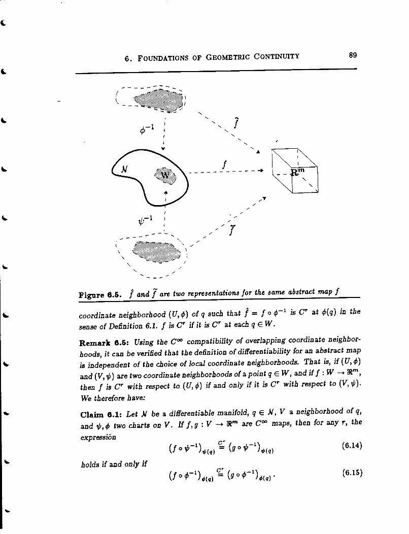
6. FOUNDATIONS OF GEOMETRIC CONTINUITY 89
--------
l
f ------------+
1/J-1 ------
\ \
/
Figure 6.5. J and J are two representations for the same abstract map f
coordinate neighborhood (U, tjJ) of q such that j = f o 1/J- 1 is cr at tjJ(q) in the
sense of Definition 6.1. f is cr if it is cr at each q E W.
Remark 6.5: Using the coo compatibility of overlapping coordinate neighbor
hoods, it can be verified that the definition of differentiability for an abstract map
is independent of the choice of local coordinate neighborhoods. That is, if ( U, tjJ)
and (V, 1/J) are two coordinate neighborhoods of a point q E W, and iff : W - ~m,
then f is cr with respect to (U, tjJ) if and only if it is cr with respect to (V, ,P).
We therefore have:
Claim 6.1: Let )I be a differentiable manifold, q E )I, V a neighborhood of q,
and 1/J, tjJ two charts on V. Iff, g : V - ~m are C 00 maps, then for any r, the
expression (6.14)
holds if and only if (6.15)
6. FOUNDATIONS OF GEOMETRIC CONTINUITY 90
In order to use the Inverse Function Theorem for maps on manifolds, the
notion of regularity must be extended to abstract maps. This we now do.
Definition 6.4: Let I: w c )I --+ ~m be a cr map, r ~ 1, )/ a. differentiable n~
manifold with n $; m. I is said to be regular at q E W if there exists a coordinate
neighborhood (U, 4J) of q such that J = I o 4J- 1 is regular at q in the sense of
Definition 6.1. I is said to be regular if it is regular at every q E W.
A regular cr map is called a cr immersion. If r = oo, then the map is called
simply an immersion. It is important to note that a cr immersion need not be
1-1. However, if a cr immersion is 1~1, then it is called a C" embedding. The next
theorem shows that immersions are locally embeddings.
Theorem 6.5: Let I : )/ --+ ~m be a cr immersion. Each p E )I has a
neighborhood U such that I restricted to U is a C" embedding. That is, f is
locally 1 - 1.
Proof: For a proof, see Boothby [14], Theorem 4.12. I
The notion of a diffeomorphism can be extended readily to abstract maps on
manifolds as follows. Let f : W --+ ~m, W C )/, and let W' be the image of li that
is W' = I(W). I is said to be a cr -diffeomorphism iff is C"' and 1-l : W'--+ w exists and is cr. The next theorem shows the connection between embeddings
and diffeomorphisms.
Theorem 6.6: If I : w --+ ~m' w c )/ is a C" embedding, then I is a crdiffeomorphism.
Proof: For a proof, see Boothby [14], Remark 4.2. I
Remark 6.6: Theorems 6.5 and 6.6 together imply that immersions are locally
diffeomorphisms.
The next theorem shows that the image of a manifold under an embedding is
itself a manifold, and is called an embedded manifold.
Theorem 6.7: Let )/ be a differentiable manifold, and let I: )/ --+ ~m be a C"
embedding, r = 1, 2, ... , oo, where dim(J/) $; m. The image of)/ under I, I(JI),
is a cr manifold.
Proof: For a proof, see Boothby [14], Chapter 4. I

6. FOUNDATIONS OF GEOMETRIC CONTINUITY 91
We will say that a manifold )/ is compact if there exists an embedding
f: )/ -+ 1Rm, for sufficiently large m, such that/()/) is compact when considered
as a subset of 1Rm. Once again, this is a narrow definition of compactness, but it
suffices f_or our purposes.
Remark 6.7: Theorems 6.5 and 6.7 together imply that the image of a cr immersion is locally an embedded manifold. That is, if I is a cr immersion
defined on )/, then for every q E )/ there exists a neighborhood U of q such that
f(U) is an embedded cr manifold. The image set !(N) is called an immersed
manifold.
6.5. Abstract Splines
As mentioned in Section 6.1, the notion of an abstract spline is useful when
developing a coordinate free measure of continuity. Intuitively, an abstract spline
is a coordinate free version of the usual notion of a spline as a piecewise map. The
general idea is to start with a manifold, "slice" it into smaller sub-domains, then
on each sub-domain define a map into Euclidean space.
In order to define an abstract spline on a manifold domain, we first introduce
the notion of a tesselation, used to slice the domain manifold into closed sub
domains.
Definition 6.5: Let P be a compact C00 manifold with boundary, let dim P = p,
and let a P denote the boundary of P. A tesselation of P {if it exists) is a finite
collection ~ of subsets of P such that:
i) Elements of~ (called sub-domains) cover P.
ii) Elements of~ are homeomorphic to Bf(O), the closure of a ball in 1RP of
radius 1 about the origin.
iii) If q E P is an interior point of some D E ~, then no other D' E ~ contains q.
iv) For every D E ~ there is a coordinate neighborhood ( U, 1/J) of P such that
D- (D n 8P) cU. U is called an extension of D.
v) If D n D' # 0, then D n D' is a differentiable manifold of dimension less than
p.
A tesselated manifold is a tuple (P, ~), P a manifold, ~ a tesselation of P.
Rem~k 6.8: Since~ is a finite collection, it can be ordered: ~ = {D1 , ... , Dt},
1 < t < oo. Also, since the elements of~ cover P, the coordinate neighborhoods

6. FOUNDATIONS OF GEOMETRlC CONTINUITY 92
{(U1, ,P1)}, U1 an extension of Di, form a basis for Int(P).
Example 8.3: Let P be the closed subset of fR2 [0, 2] x [0, 2], and let ~ =
{D1 , D2 , D3 , D4 } be a rectangular tesselation of P. In particular, let D1 =
[0, 1] x [0, 1], D2 = [0, 1] x [1, 2], D3 = [1, 2] x [1, 2], and D4 = [1, 2] x [01 1]
(see Figure 6.6). Note that D1 and D2 intersect in a 1-manifold (a straight line),
and D1 and D3 intersect in a 0-manifold (a single point). It is easily verified that
~ forms a tesselation of P; hence, (P, ~) is a tesselated 2-manifold. •
( 0, 2) ___ ""!""-__ __,
(0, 1) 1------+------t
(0,0) (1,0) (2,0)
Figure 6.6. A rectangular tesselation of the manifold [0, 2] x [0, 2].
Definition 6.6: Let ( P, ~) be a tesselated manifold, with ~ = { D 1 , ••• , Dt}.
Associate with each Di E ~ a C00 map s, : U, -+ alm, U, an extension of Di.
Define a piecewise map S : Int( P) -+ ~m as
S(q) = s,(q), q E Int(P), i = min{ijq E D; }. (6.16)
S is called an abstract spline on (P, ~); S is said to be given by the collection
{si, D,}. Sis said to be regular if each of the Si is regular.
It is easy to show that Sis indeed a map on lnt(P) (see Figure 6.7). However,
until we impose some restrictions on the maps Si, S need not be differentiable or
even continuous. To investigate the form of these restrictions, let S be a spline on
(P,~) given by {si,Ds}, and let q be a point on Int(P) that is on the boundary
between D 1 and D2 , but not on the boundary of any other sub-domain. We ask
the question: If sis cr at q, what does that imply about the relationship between

6. FOUNDATIONS OF GEOMETRlC CONTINUITY 93
Figure 6.7. If q E Int(P) is on the interior of a sub-domain Di, then the value
of the splineS is Si(q). If q is on the boundary between one or more sub-domains,
the map on the sub-domain of least index is used to define the value of S(q). In
the figure above, q is on the boundary between D1, D2 , and D3 , so S(q) = s1(q).
8t and 82? The fact that s is cr at q implies that there exists a coordinate
neighborhood (W, ..\) of q such that the representation of S relative to (W, ..\) is cr .....
at ..\(q). If S denotes this representation, then
S(z) =So ..\-1 (z), zE ..\(W) (6.17}
where §is cr at ..\(q) (see Figure 6.8}.
Since S is defined as a piecewise map, so is S. Specifically,
(6.18}
By definition, Sis cr at ..\(q) if and only if all partial derivatives up to order r .....
exist and are continuous at ..\(q). Equivalently, S is cr at .A(q) if and only if
( \ -1) cr ( \ -1) 81 o A .\(q) - 82 o A .\(q) • (6.19)
In general, any number of domains can contain q. The next claim handles the
general case. It can be proved by using an analysis identical to the one used
above.

6. FOUNDATIONS OF GEOMETRIC CONTINUITY
1).. I
.>..(W) --..,-- -------/
I
\ .>..(Dd \ .>..( q)
---
/
/
/
/
I /
Jf /
/
,.. s
94
Figure 6.8. The representation of a spline S relative to a coordinate neighborhood
(W, ~) for a point q E Int(P) on the boundary between D1 and D2 •
Claim 6.2: Let S be an abstract spline on ( P, ~) given by { Si, Di}, and let
(W, ~) be a coordinate neighborhood of q E Int(P). Let S(x), x E W, denote the
representation of S relative to (W, ~):
..... -1 S(x) = Si o ~ (x), i = min{jlx E ~(D,.)},
.... and let Di 1 , ••• , Di,. be all domains containing q. Sis C" at A(q) if and only if
( ,-1) cr ( ,-1) c~ cr ( ,-1) Si1 o A ~(q) = Si2 o A ~(q) = · · · = Si,. o" ~(q) {6.20)
Remark 6.9: Expression (6.20) holds if and only if it holds on a pairwise basis.
Abstract splines are convenient theoretic tools, but in practice we must deal
with representations. The representation S in Claim 6.2 is an example of a local
representation of S. The representation is local in the sense that it is only valid
for the .neighborhood W of q. A global representation of S can be considered to
be a collection of local representations. Of course, there are many possible global

6. FOUNDATIONS OF GEOMETRlC CONTINUITY 95
representations, but there is a class of global representations that is particularly
useful in practice. The idea is to use global representations that consist of a
collection of representations of the maps Si· We now formalize this idea.
Let !J be a subset of lRP that is homeomorphic to B~(O), let fJ be an open
subset of lRP containing /J, let x = (x1 , ••• , xp) be a coordinate system on fl, and A ~
let s(x) be a. coo function from U into lRm. s, when restricted to D, is called a
parametrization., and is said to be parametrized on. D. The tuple (s, D) is used to
denote a parametrization s parametrized on D.
Definition 6.7: LetS be an spline on (P,~) given by {si,Di}· Let (Ui,tPi) be
a coordinate neighborhood such that Si is defined on Ui, for Ui an extension of
Di. A parametrization (si, Di) is said to be a parametrization. for Si relative to
(Ui, tPi) if (6.21)
and Di = ,P(Di)· That is, Si is a representation of Si relative to (Ui, tPi)·
Conversely, Si is said to be a lifting of (si, Di) relative to (Ui, tPi)· The coordinate
neighborhood ( Ui, tPi) is called a connecting neighborhood (intuitively, it "connects"
si and (si, Di)).
Let S be as above, and let {(Ui, t/Ji)} be a collection of coordinate neighbor
hoods such that Si is defined on ui, ui an extension of Di. A parametric represen
tation. of S relative to {(Ui, t/Ji)} is a collection of parametrizations {(si, Di)} such
that for each i, Si is a lifting of ( Si, Di) relative to ( Ui, tPi). The set of connecting
neighborhoods {( Ui, tPi)} relating S and {( Si, Di)} is called a connecting basis.
A collection { ( Si, Di)} is said to be a parametric representation. on. (P, ~) if
the collection is a parametric representation of some abstract splineS on (P, ~).
Conversely, S is said to be a lifting of {(si, Di)}.
6.6. Parametric Splines
As mentioned in Section 6.1, a parametric representation is "lifted" onto
the manifold to define a coordinate free abstract spline. However, not just any
coll~ction of parametrizations forms a parametric representation. The parametric
domains, when lifted onto the manifold, must fit together (without overlapping) to
cover the manifold. The next example should help to clarify some of these ideas.
Example 6.4: We examine the relationship between a parametric representation
and an associated abstract spline for the surface shown in Figure 6.9. We begin

6. FOUNDATIONS OF GEOMETRlC CONTINUITY 96
by discussing the construction in the old language of Chapter 2, and then show
how the construction relates to the new language of abstract splines on manifolds.
The surface shown in Figure 6.9 is represented by the four parametrizations
81 , 8:;11 83 , and 84 • § 1 is parametrized on [0, 1] x [0, 2], 82 on [0, 2] x [0, 2], and sa and 84 on [0, 1] x [0, 1].
I
I
I
I
I
sl (1 ,2)=s2(2,2)=s3(o,o)=s 4(o, 1)
Figure 6.9. A spline surface consisting of four patches generated by 81 , 82, 83
and 84 •
As demonstrated in Section 2.5, if the surface is to be continuous (C0 ), a
set of correspondence maps must be established that relate parametric boundary
points . . We choose the simplest correspondence maps consistent with the situation
shown in Figure 6.9. The correspondence map between 81 and 84 is is partially
established by Figure 6.9 in that the point 81 ( 1, 0) is associated with the point
84 (0, 0), and 81 (1, 2) is associated with 84 (0, 1). Equivalently, (1, 0) in 81 's domain
is associated with (0, 0) in 84 's domain, and (1, 2) in 81 's domain is associated with
(0, 1) in 84 's domain. Let (u1 ,v1 ) be the coordinate system on 81 's domain, and
let ( u4 , v4 ) be the coordinate system on 84 's domain. The simplest correspondence
along the 811 84 boundary consistent with Figure 6.9 is therefore
u4 = u 1 -1
1 t/4 = -til·
2
(6.22)

6. FOUNDATIONS OF GEOMETRlC CONTINUITY
Similarly, the simplest correspondence along the 82,53 boundary is
t£3 = tJ2- 2 1
t13 = 2(2 - '-'2)
97
(6.23)
where ( '-'2, v2 ) and ( u3, v3 ) are coordinates systems on the domains of 82 and 83,
respectively (note that even the simplest corre:Jpondence of equation (6.23) mixes
the u's and v's of the coordinate systems). The correspondences for the remaining
two boundaries can be determined in a similar fashion.
The C0 condition along the 81 , 84 boundary can now be stated as
81(1, vi)= s4(u4 = 1- 1, tJ4 = ivd = 84(0, !vi)
2
(6.24)
for all v1 E [0, 2]. Similar expressions for the other boundaries can be obtained
analogously, thus completing the construction of a C0 ~urface in the old language.
To demonstrate how the parametric representation given above can be lifted
onto a manifold, we choose a tesselated manifold that admits an abstract spline
having { 81 , 82 , 83 , 84 } as a parametric representation. In particular, we choose the
tesselated manifold of Example 6.3, lifting 51 onto D 1 , 82 onto D2 , and so on. We
must now choose a connecting basis; i.e., the coordinate neighborhoods ( U1 , 1/11),
(U2, t/;2), (U3, t/;3), and (U4, 1/14) relative to which the lifting will occur. For the
extensions ul, u2, u3, u4, simply choose Ut = u2 = u3 = u4 = (0, 2) X (0, 2). St
is parametrized on [0, 1] x [0, 2], so t/;1 must be such that ,Pl(Dt) = [0, 1] x [0, 2].
Similarly, t/J2(D2) = [0, 2] x [0, 2], t/;3(D3) = [0, 1] x [0, 1], and t/;4(D4) = [0, 1] x [0, 1]
(see Figure 6.10).
The fact that (1, 0) in 81 's domain is associated with (0, 0) in 84's domain
means that (1, 0) and (0, 0) are images of the same point on the manifold. In other
words, the same point on the manifold, and hence the same point on the spline
surface, is given a different coordinate assignment relative to different coordinate
systems, or equivalently, relative to different parametrizations. The conversion
from 81 's coordinate to 84 's coordinate for a point on the 81 , 84 boundary is given
by equation (6.22). In the new language, this correspondence map describes the
transition function t/;4 o ¢11 restricted to the u1 = 1 edge of 51 's domain. Thus,
the C0 condition of equation (6.24) can be rewritten in the new language as
(6.25)

6. FOUNDATIONS OF GEOMETRlC CONTINUITY 98
,. 81 /
2 ~
I -~D \ \
0 81 84 \
0 1 I .. ~
\ I
' D2 D3 \
,' tP4
' / /
/ /
' /
tP1 ' /
' Dl D4 '
Figure 6.10. The relationship between the manifold1 the parametrizations1 and
the abstract spline.
Equation (6.25) can be written in terms of abstract maps s1 - 81 o V;1 and
s4 = 84 o ,P4 as
(6.26)
Equation (6.26) is therefore tbe coordinate free form of continuity between 81 and
84 • Tbe parametrizations s~ and 83 can be lifted in a similar manner. • Example 6.4 shows that when building splines in practice, one begins with a
collection of parametrizations, together with a set of correspondence maps that
ensure CO continuity. Our definition of a parametric spline, that is, a spline that is
constructed in practice, should contain this information. There are many possible
definitions that capture this information. The most obvious definition would be
to treat a parametric spline as a collection of parametrizations together with a
set of correspondence maps. Although conceptually simple, this definition does
not seem to be particularly convenient for a theoretical study. The definition of a
parametric spline we will ultimately use is rather esoteric, so we begin with some
motivational observations.

6. FOUNDATIONS OF GEOMETRIC CONTINUITY 99
Notice that the abstract spline in Example 6.4 is not uniquely defined since
the charts with respect to which the lifting oq::urred were not unique; any other
connecting basis consistent with the correspondence maps could ha.ve been used.
Intuitively this means that a given parametrlc representation represents many
abstract splines consistent with a fixed set of correspondence maps. To investigate
this further, let S be a CO abstract spline on (P, ~),let {(s;, D;)} be a parametric
representation :-elative to the connecting basis {(Ui,..tPi)}, let q be a point on
the manifold common to the sub-domains D; and n,., and let (U;,,P;), (U;,,P;)
be the connecting neighborhoods that are associated with Di and D;. Thus,
,P;(D1) = D; and t/J;(D;) = D;. As shown in Example 6.4, the point ,P;(q) in .D, is _associated with the point ,P;(q) in D;. In this way, a connecting basis uniquely
determines a set of correspondence maps. However, the converse is not true - a.
set of correspondence maps does not uniquely determine a connecting basis. In
particular, let ,P~ be a chart on U, such that
1) ,P;(D;) = ,P;(D,)
2) t/JHq) = ,P;(q), for all q E an,. (6.27)
That is, tPi and t/Ji behave identically on the boundary of D;. Two charts satisfying
properties 1 and 2 of equation (6.27) are said to be similar (actually, 2 implies 1
since D; is homeomorphic to B~(O)). The interesting thing about similar charts
is that they preserve correspondence maps. That is, ,P1(q) corresponds to ,P;(q) if
and only if ,P;(q) corresponds to tPi(q). In addition, properties 1 and 2 of equation
( 6.27) imply that s; can be lifted relative to ( U,, t/JD to describe the abstract map
s~ = §;o,P~. The abstract maps~ is therefore related to the abstract maps; = §iotPi
(defined by the connecting basis), according to
I .1,-1 .1,1 Si = Sj o 'l'i o 'l'i· (6.28)
Equation (6.28) shows that Si is a representation of s, relative to t/;1, as well
as being a representation of s~ relative to ,P~. Two abstract maps are said to be
similar if they are related by similar charts as indicated by equation ( 6.28). Two
splines S and S', given by { s,, Di} and { s~, Di} are said to be similar if for each
i, s, is similar to s~. Note that if S and S' are similar, then they have a common
parametric representation, and if { ( Si, .D,)} is a parametric representation, it is
relatively easy to show that "similarity" is an equivalence relation on the set of
abstract splines represented by { ( s,, .D,)}.

6. FOUNDATIONS OF GEOMETRlC CONTINUITY 100
The important point of the above discussion is that a parametric representa
tion and a set of correspondence maps determines an abstract spline only up to
similarity. This observation is the basis of our definition of parametric splines.
Definition 6.8: Let {(si, Di)} be a parametric representation on (P, ~), let S
be a C0 lifting of {(si, .D .. )}, and let C be the ~quivalence class of abstract splines
similar to S. The tupleS= ( {(si, Di)}, C) is called a parametric spline on (P, ~); S is said to represent S' if S' E C; Sis said to be regUlar if each of the maps Si is
regular on Di. We will often be lax and use the term "spline" to be synonymous
with "regular parametric spline".
Remark 6.10: With each S E C, there is an associated unique connecting basis
relating S and {(si, Di)}. Thus, an equivalent deBnition of a parametric spline is
a tuple ( {(si, Di)}, E), E an equivalenc~ class of similar connecting bases. Similar
connecting bases are defined in the obvious way: two connecting bases {(Ui, tPi)}
and {(Ui, t/1~)} are called similar if for each i, tPi is similar to .p;. In fact, given
any two of C, E and {(si, Di)}, the third is uniquely determined. Unfortunately,
none of the (;) possible definitions seems to be superior in all cases.
Notation: Let S = ( { ( Si, Di)}, C) be a parametric spline on ( P, <b). We use the
notation S: Int(P) --+ 1Rm to mean that the abstract splines represented by S are
maps from Int(P) into lRm. In a similar spirit, we take S(Int(P)) to be the set
S(Int(P)), SEC.
As a follow up to Remark 2.2, it is important to realize that the assumption of
CO continuity has been woven into the definition of a parametric spline by requiring
allliftings to be C0 abstract splines. The CO assumption is very convenient when
working on the manifold. As a specific example of the difficulties encountered when
the C0 assumption is not made, consider the situation depicted in Figure 6.11.
The parametric domains D1 , D2 , and D3 are to be lifted onto the manifold [0, 3],
tesselated into the sub-domains [0, 1], [1, 2], and [2, 3]. Since all closed intervals
are diffeomorphic to one another, it is possible to lift any of the .Di onto any
of the sub-domains. In fact, each of the liftings can be performed in either of
two possible ways. Without the C0 assumption, it is unclear which of the many
liftings will result in a C0 spline; three possibilities are shown in Figure 6.11. In
Figure 6.1l(a), D1 and D2 are "adjacent" on the manifold, with the point 1 E D1
corresponding to 0 E D2 • D1 and D2 are again adjacent in Figure 6.11(b), except
that 0 E D1 corresponds to 0 E D2 • In Figure 6.11(c), D1 and D2 aren't even
adjacent. Thus, without the C0 assumption, even the notion of adjacency is lost.

6. FOUNDATIONS OF GEOMETRlC CONTINUITY 101
However, when one constructs splines in practice, there is a very definite idea
of which parametrizations are to be treated as adjacent - the CO assumption
provides this structure while still allowing cross boundary freedom.
0 1 2 3
(a) ..
~1 --~1 ~i --~11 ~ --~l 0 1 0 1 0 1
0 1 2 3
(b)
0 1 0 1 0 1
0 1 2 3
(c) :.-·
1-j -.......;\"" 1~--~1 ]1------1\
0 1 0 1 0 1
Figure 8.11. Three possible liftings of [0, 1], [0, 1], [0, 1] onto the tesselated
manifold ([0, 3], {[0, 1], [1, 2], [2, 3]} ).
6. 7. Weak Geometric Continuity, war Splines
As mentioned previously, an equivalence class of abstract splines is used to
stitch the domains of a parametric spline together to achieve CO continuity. The
goal is now to determine parametrization independent constraints on the Bi that

6. FOUNDATIONS OF GEOMETRIC CONTINUITY 102
are necessary and sufficient for higher order differentiability of an abstract spline
S represented by the parametric spline. This can be achieved by:
1) Lifting the representations Si onto the manifold P to obtain abstract
maps Si·
2) Using the usual definition (Definition 6.3) of continuity for a map on a
manifold. Since this is a measure of continuity that holds independent
of the local coordinate system, it is independent of the representation of
the s,. 3) Restate the constraints on the manifold in terms of the parametrizations
The underlying mathematical structure -of a parametric spline provides the key to
step 1, and step 3 is simply the inverse of step 1. The key to step 2 is provided by
Claim 6.2, so we must simply put the pieces together, a task we now undertake.
It was shown above that equation (6.19) is a necessary and sufficient condition
on the abstract maps s1 and s2 if S is to be cr. From Claim 6.1, we see that
equation (6.19) is a coordinate independent statement- it is therefore the key to
a parametrization independent measure of continuity for splines. Formally:
Deflnition 6.9: Let S = ( { ( Si, Di)}, C) be a regular parametric spline on ( P, ~), and let S be a lifting of S relative to {(Ui, t/li)}. The parametrizations Si and s; are said to abut atq ifq E DinD;. Si and 8; aresaid to abut on V ifV C DinD;.
Let S be as above, let Si and s; abut on V, and let Si = Si o t/li, s; = s; o t/1;, then:
• Si and s; are said to meet with WGr continuity at q E V with respect to S if
(6.29)
• Si and s; are said to meet with WGr continuity at q E V if there exists a
lifting S with respect to which they meet WGr at q.
• S is said to be a WGr spline at q with respect to S if all parametrizations
abutting at q meet with WGr continuity at q with respect to S.
• S is said to be a WGr spline on ( P, ~) if there exists a lifting S with respect
to which Sis WGr at all q E Int(P).
We call this "weak" geometric continuity because no stipulations have yet
been made concerning orientation. The orientation preserving conditions will be
developed in Section 6.8.

6. FOUNDATIONS OF GEOMETRlC CONTINUITY 103
Remark 6.11: In Remark 2.1, it was pointed out that there is a possible alternate
definition for two parametrizations meeting with geometric continuity on a set.
Within the framework of manifolds, and using the definition above for Si and
§:i meeting with WGr continuity at a point q, an analogous definition for weak
geometric continuity may be stated as: Si and §,- meet with W G" continuity on
W C V if they meet with W Gr continuity at ali q E W. This definition of W Gr
on a set allows the lifting used at q1 E W to differ from the lifting used at q2 E W.
It is conjectured that the two definitions are in fact equivalent, but a proof has
not been constructed.
The alternate definition bas the advantage that continuity on a set can
be guaranteed by individually establishing continuity at each point of the set,
eliminating a consideration of the set as a whole. Thus, the alternate definition
is better suited to proving Theorem 6.12 (the Beta constraint theorem), and the
equivalence theorems given in Section 6.10. We have chosen to adopt Definition 6.9
because it expedites the proofs of the theorems detailing the smoothness of the
images of War splines (Theorems 6.8 and 6.9 ).
The next lemma establishes several minor (but useful) equivalent definitions of
weak geometric continuity at a point. In particular, it shows that Definition 6.9 is
reflexive in the sense that tf;; could have been used instead of t/Ji in equation (6.29).
In Section 6.10, additional equivalent definitions are proven.
Lemma 6.1: LetS= ({(si,Di)},C) be a parametric spline on (P,~), and let
S be a lifting of S relative to { ( Ui, t/Ji)}. The following expressions are necessary
and sufficient conditions for WGr continuity of si and s; with respect to S at q:
(6.30)
(sdw.(q) ~ (si o t/J; o ¢;1 )w.(q) ( 6.31)
( A ) cz ( A olo olo -1 ) Sj WJ(q) - Si o 'l'i o 'l'j tPj(q) {6.32)
where Si = Si o t/Ji and Sf= Sf o tPi·
Proof: Equation (6.30) follows immediately from equation (6.29) and Claim 6.1.
Equation (6.31) follows from (6.29) by first using the fact that §i = Si o t/Ji 1•
Specifically, ( 6.29) can be rewritten as
(6.33)

6. FOUNDATIONS OF GEOMETRJC CONTINUITY 104
Now, rewrite the right side of (6.33) by inserting the indentity in the form of
t/Jjl 0 VJ:i:
(si)t/l·(q) cr (s:i 0 1/Jj1 0 tP:i 0 t/Ji1
) 0
• W;( q) (6.34)
Equation (6.34) can now be written 3.8 equation (6.31) by using s:i = s:i o ,Pj1•
Equation (6.32) follows from (6.30) in the same way as (6.31) followed from
(6.29). I
Let us digress for a moment to make a few comments concerning parametric
continuity. Recall that parametric continuity, as introduced in Chapter 2, requires
that parametric derivatives agree at common points between parametrizations, In
the language of manifold theory, parametric continuity may be stated as follows.
Definition 6.10: Let Si and s:i be as in Definition 6.9. They meet with parametric
continuity of order r rcr) on v if they meet with war on v and the Jacobian
matrix of VJ:i o t/Ji 1 is the identity matrix.
Definition 6.10 shows that parametric continuity is very restrictive. It
essentially states that Bi and s:i must share the same parameter space, or
equivalently, the same local coordinate system. Thus, parametric continuity is
a concept that is clearly not coordinate independent.
Remark 6.12: The important point fs this: In the old language, parametric
continuity seemed natural, and geometric continuity was developed as a rather
subtle extension. However, in the new language of manifolds we start with a
coordinate free framework. In that framework, geometric continuity is natural,
and parametric continuity is a subtle special case.
In this section, the notion of a war spline has been introduced as the
type of spline that results when parametrizations are stitched together with weak
geometric continuity. We now wish to characterize the behavior of these splines
by examining the smoothness properties of their images. After all, it is the image
of the spline that is relevant in CAGD. The next lemma. a.nd theorem show that
WGr splines a.nd cr immersions (introduced in Section 6.4.2) a.re, in a. sense to
be defined, really the same thing.
Lemma 6.2: LetS= ( {(.Si, Di)}, C) be a spline on (P, 4>). S represents a regular
cr map at q E Int(P) if and only if S is a WGr spline at q.

6. FOUNDATIONS OF GEOMETRlC CONTINUITY 105
Proof: Let D;1 , ••• , D;k be all sub-domains of~ containing q. We begin by assuming -that S represents a regular cr map at q, meaning that there exists an abstract
spline S E C that is a regular cr map at q. Let S E C be such an abstract
spline, and let {(U;, 1/1;)} be the connecting basis relative to which S is a lifting
of {(s;,D;)}. sis therefore an abstract map given by {s;,D;}. Since sis cr
at q, Definition 6.3 implies that there exists a coordinate neighborhood (W, .A) of
q such that S(x) = s 0 A- 1 (x), X E A(W) is cr at A(q). Due to the coordinate
independent nature of differentiability, this must hold for any chart A defined on
W. From Claim 6.2 and Remark 6.9, it must be that
(s;oA-l)~(q) cr (s;oA-l)~(q) (6.35)
holds for every pair of indices i, j chosen from {i1, ... , ik}· Now, restrict attention
to an open subset
v = w n U; 1 n U;, · · · n uik.
Since V is a subset of W, equation (6.35) must also hold for any chart defined on
V. In fact, V has been chosen so that each of the charts 1/1; 1 , ••• , 1/l;k is defined on
V. In particular, let A = 1/J;, the chart associated with 8;. Equation (6.35) relative
to 1/1; becomes (6.36)
which by Definition 6.9 means that s;, s; meet with WGr continuity at q. The
pair i, j was chosen arbitrarily so it must hold for every pair. By Definition 6.9,
S is therefore WGr at q.
To prove the converse, assume that Sis WGr at q, implying that every pair
8;, 8; abutting at q meets with WGr continuity at q with respect to some S E C.
Let S be such a lifting of S relative to {(U;, 1/1;)}. We must show that there exists
a coordinate neighborhood (W, A) of q such that S relative to (W, A) is regular and
cr at A(q).
Let W = U; 1 n · · · n U;k. On W, all the charts 1/1;1 , ••• , 1/l;k are defined;
arbitrarily choose 1/1;1 • By assumption, every pair s;• = s;• o 1/1;•, s;' = s;• o 1/1;•
from { s; 1 , ••• , s;k} satisfies
(s;• o ,p~l)t/1;1(q) g (si' o ,p~l)t/1;1(q). (6.37)
By Claim 6.2, S =So 1/1~ 1 must be cr at 1/1;1 (q), which in turn implies that Sis
cr at q. Regularity follows from regularity of the s's. I
Theorem 6.8: Let S be as in Lemma 6.2. S represents cr immersion on ( P, ~)
if and only if it is a WGr spline on (P, ~).

6. FOUNDATIONS OF GEOMETRIC CONTINUITY 106
Proof: This follows immediately from the definition of a C" immersion, Defini
tion 6.9 for war splines, and Lemma 6.2. I
Remark 6. 7 and Theorem 6.8 together imply that the image of a WG" spline
is a C" immersed manifold. Moreover, if the spline is 1-1 as well as being WGr 1
then its image is an embedded cr manifold. This provides further confidence that
(weak) geometric continuity is a desirable measure of smoothness for the image of
a spline. The next theorem and the remarks thereafter provide even more evidence
of the smoothness of war splines.
Theorem 6.9: Let S : Int(P) -+ !RP+l be a parametric spline on (P, ~),
dim(P) = p, and letS be a lifting of s. Sis a war spline if and only if S(Int(P))
is locally the graph of a cr function. That is, S is Wa" if and only if for every
q E Int(P), there exists a neighborhood U of q, a neighborhood U' of S(q), and a
coordinate system (x1 , ... , Xp+t) for !RP+l, such that
(6.38)
for some cr function f.
Proof: This theorem is proved in most texts on manifold theory for the case of a
cr immersion. Since war splines represent immersions, the same proof holds true
here. For the complete proof for immersions, the reader is referred to Boothby [14]. I ,
The case p = 1 in Theorem 6.9 corresponds to war spline curves in two
space. We therefore have as a corollary to Theorem 6.9: The image of a war spline curve in two-space is locally the graph of a cr function f(x). Intuition
developed in calculus leads us to believe that graphs of differentiable functions
are smooth; hence, the image of a war spline is smooth. Another corollary to
Theorem 6.9 corresponds to p = 2, and may be stated as: The image of a WGr
spline surface in three-space is locally the graph of a cr bivariate function f(x, y).
Once again, intuition from calculus suggests that the images of war spline surfaces
are also smooth.
6.8. cr Splines
We now move from war continuity to cr continuity by maintaining orienta
tion information. This is done by requiring the connecting bases to be oriented.

6. FOUNDATIONS OF GEOMETRlC CONTINUITY 107
Definition 6.11: LetS= ({(si,Di)},C) be a spline on (P,~), letS E C be a
lifting relative to {(Ui, tPi)}, and let Si and s; be two parametrizations abutting
at q E Int(P).
• Si and s; are said to meet with cr continuity at q with respect to S if they
meet with WGr continuity at q with respect to S and (Ui, tPi) and (U;, t/1;)
are coherently oriented.
• Si and s; are said to meet with cr continuity at q if there exists a lifting S E C
with respect to which they meet with cr continuity at q.
• S is said to be cr at q with respect to S if every pair of parametrizations
ab'}tting at q meet with cr continuity at q with respect to S.
• S is said to be a Gr spline (on ( P, ~)) if there exists a lifting S E C with
respect to which Sis Gr at every q E Int(P).
The old language can be viewed as keeping the abstract spline fixed, while
wandering through equivalent parametrizations to find some that meet with pa
rametric continuity. On the other hand, the new view is to keep the parame
trizations fixed, while wandering though the abstract splines. As will be shown in
Theorem 6.10, the two views are equivalent when considering continuity between
two parametrizations, but it is difficult to imagine how the old language would
handle a entire collection of parametrizations. In the n€W language, a collection of
parametrizations presents little difficulty since the manifold is used as a common
platform on which the parametric domains are to be related.
In Chapter 2, reparametrization played an important role in the development
of geometric continuity. In the new language, we say that two parametrizations
(s, D) and (8, D) are GO-equivalent if there exists an orientation preserving
diffeomorphism d: D-+ D such that 8-. sod. More generally, we can say that they
are weakly GO-equivalent (WGO-equivalent) if there is a diffeomorphism relating
them, irrespective of its orientation properties. To develop some intuition for the
formal mathematical structure of a parametric spline, the reader is encouraged to
prove the following lemma as an "exercise".
Lemma 6.3: Let S = ( {(si, Di)}, C) be a regular parametric spline on (P, ~),
and let { (s;, Di)} be a collection of parametrizations such that, for each i, s; is
WGO-equivalent to s;. Show that S' = ( {(s;, Di)}, C) is a spline on (P' ~).
Proof: Let S E C be a lifting of {(si, Di)} relative to {(Ui, tPi)}. Relative to this

6. FOUNDATIONS OF GEOMETRIC CONTINUITY 108
connecting basis, §i represents the abstract map
(6.39)
By assumption, {(si, Di)} is a collection of parametrizations such that for each i,
Si = Si o di, di a diffeomorphism such that di(D) =D. Define a map tPi by
(6.40)
By construction, tPi is compatible with 1/Ji, hence <Pi is a chart. From (6.39} and
(6.40}, we see that Si = §i o 1/J; = Si o <Pi, implying that Si is a lifting of Si relative
to tPi. This must be true for every i, so S is a lifting of { (si, Di)} relative to
{(Ui, <Pi)}. S is a representative of the equivalence class C, so S' = ( {(si, Di)}, C)
is a spline on (P, ~). I
Note that S and S' of Lemma 6.3 are alike in the sense that they represent
the same equivalence class of abstract splines, and therefore have the same image.
Howeve·r, they are different in the sense that they provide a different parametric
representation for the equivalence class, implying that the correspondence maps
differ.
The next theorem establishes the equivalence of the new and old views for
continuity between two parametrizations.
Theorem 6.10: Let S = ( { ( Si, Jji)}, C) be a regular parametric spline on ( P, ~),
and let si, 8; be abut on V c P. §i and 8; meet with war continuity on V
if and only if there exist WOO-equivalent parametrizations Si and 83·, belonging
to a spline S' = ( {(si, Di)}, C) on (P, ~), that meet with cr continuity on V.
Moreover, Si and s; meet with ar continuity on V if and only if there exist GO
equivalent parametrizations that meet with cr continuity.
Proof: We begin by assuming that si and 8; meet with war continuity on V,
implying that there exist connecting neighborhoods (Ui, 1/Ji) and (U;, 1/J;) such
that (6.41)
Let 1/J; be a chart on U; such that tPi o t/Ji 1 is the identity map on 1/Ji(Ui n Ui)
(such a chart must exist). Let (s;, D;) be a parametrization defined by
~ A o/o ,;.-1 s; = s; o '~'i o '+'j (6.42)

6. FOUNDATIONS OF GEOMETRlC CONTINUITY 109
where D; = 1/J; o <Pj 1 (D; ). Since 1/J; o <Pj 1 is a diffeomorphism, s; and s; are
WGO-equivalent. Solve equation (6.42) for s; and substitute into (6.41) to yield
\fq E V. (6.43)
Since i; is WGO-equivalent to 8;, and since Si is WGO-equivalent to itself, by
Lemma 6.3, s; and Si belong to another spline S' on (P' ~). By construction,
<P;o1/J; 1 is the identity map, so by Definition 6.3, Si and s; meet with cr continuity
on v, thus completing the proof of necessity for war continuity.
The proof of necessity of ar continuity is identical to the proof above, except
it must be shown that 1/J; and <P; are coherently oriented, given that 1/Ji and 1/J;
are coherently oriented. This can be done by letting q be any point in V, and
noting that J[ tPi o 1/Jj 1 ] ( 1/Ji( q)) is positive by assumption. The following derivation
establishes the coherent orientation of <P; and 1/J;:
J[<P; 0 1/Jj 1 ](1/Ji(q)) = J[(1/Ji 0 1/Ji 1) 0 <P; 0 1/Jj1](1/Ji(q))
= J[t/li 0 t/Jj 1](t/li(q))
> o,
(6.44)
The second line in equation (6.44) follows from the first line because 1/Ji" 1 o <P; is
the identity by construction.
To prove sufficiency, assume that Si and s; belong to a spline S' -( { (si, Di)}) C) such that Si and s; meet with cr continuity on v' and that Si
and i; are WGO-equivalent to Si and s;, respectively. Let Si and s; be liftings of
Si and Sj with respect to which they meet with cr continuity, and let <Pi and <Pi
be the corresponding charts. That is,
- ..~.-1 Si = Si o 'T'i - A,-1 s; = s; o 'T'j
(6.45)
where
( -) ~ (- A. • ..~.-1) Si <fli(q) - s; o 'T'i o 'T'i </l;{q), \fq E V (6.46)
and J[<P; o <Pi 1 ](<Pi(q)) = 1. WGO-equivalence implies the existence of diffeomor
phisms di and d; such that
(6.47) - A d s; = s; o i·

6. FOUNDATIONS OF GEOMETRlC CONTINUITY
Let .p, and tPi be new charts on U;. and U; defined by
tPi = d, 0 tPi
tPi = d; 0 tPi·
110
( 6.48)
With these definitions, Si and s; are liftings of s;, and Sj relative to (U;., t/Js) and
(Uj, t/J;). That is, A .t.-1 Si = Si o 'Yi
s; = s3 o .p-;1 • (6.49)
Write equation (6.46) in terms of Si and si using equation (6.45), then use
Claim 6.1 and Lemma 6.1 to obtain
(6.50)
showing that s, and s; meet with WGr continuity on V. Moreover, if 8;. and si are
GO-eq~ivalent to s;. and s;, then J d;. > 0, J d; > 0, and J[ tPi o tPi 1 ] = 1, implying
J[t/J; 0 t/Ji 1] = J[(di 0 tP;) 0 (di 0 cPi)-1
]
= J[di 0 cPi 0 4>i 1 0 di
11
= Jd; J[4>i 0 tPill Jdjl
> 0.
(6.51)
Thus, tPi and tPi are coherently oriented, meaning that s;. and s; meet with Gr
continuity on V. I
It is natural to ask what kind of manifolds allow Gr splines to be constructed
on them. The next lemma shows that Gr splines dm only be constructed on
orienta.ble manifolds.
Lemma 6.4: If Sis a Gr spline on (P, ~), then Int(P) is an orientable manifold.
If Int(P) is not orientable, then it is not possible to construct a Gr spline on P.
Proof: To prove the first statement, let s be a ar spline on (pI ~)I implying the
existence of a connecting basis {(Ui, t/J;.)} that is coherently oriented. Since the
connecting basis is a basis for Int(P), Int(P) must be orientable.
To prove the second statement, assume that Int(P) is not orientable, and
let ~ be an arbitrary tesselation of P. Now, assume there exists a Gr spline S on (P, ~). By the proof of the first statement, Int(P) is orientable, which is a
contradiction. I

6. FOUNDATIONS OF GEOMETRlC CONTINUITY 111
ar splines provide a natural orientation for the image of the spline. To
investigate this, let s = ( {(.Si, Di)}, C) be a ar spline on (P, ~), r ~ 1, with ~
dim(P) = p. Let Si and Sf be two parametrizations of S that abut at some point
q E Int(P), and let tPi and tPi be the charts relative to which they meet with
ar continuity. Consider the Jacobian matrix of .Si evaluated at q. To evaluate
Si at a point q on the manifold, q must be expressed in terms of the coordinate
neighborhood (Ui, tPi)· Thus, the Jacobian matrix of interest is D.Si( tPi(q)). Each
of the p columns of this matrix can be thought of as a vector in !Rm, and since
Si is assumed to be regular, the columns are linearly independent. The columns
considered as vectors therefore span a vector space of dimension p. In fact, the
vector space they span is called the tangent space of the image of Si at .Si(tPi(q)),
denoted Tt/li(q) (.Si)·
Example 6.5: An example of a tangent space was discussed in Section 2.5,
although it wasn't identified as such. In that section, the partial derivatives
G ( 1•0 ) (up, tip) and G ( 0 •1 ) (up, tip) were shown to span the tangent plane of G
at p (more precisely, they span the tangent plane of the image of G at the point
p). To see the connection to the defintion of a tangent space above, note that
the components of the vectors Gll,O) and G(O,l) are the columns of the Jacobian
matrix DG( up, tip)· For surfaces, the tangent space is two dimensional, and is
therefore called the tangent plane. Thus, the columns of DG( up, tip) span the
tangent space Tp(G). •
Prior to Example 6.5, we saw that the columns of Dsi(tPi(q)) span Tt/l;(q)(.Si)·
Similarly the columns of the Jacobian matrix of Sf span Tt~~1 (q)(s,.). Recall that
Si and Sf meet with ar continuity at q with respect to tPi and ,p,., implying that
the first order partials of Si ~t q and the first order partials of .s,. o tPi o t/Ji 1 at q
agree. This condition can be written in matrix form as
(6.52)
which by the chain rule (Theorem 6.1) can be written as
(6.53)
The matrices D.Si(tPi(q) and Ds;(,P,.(q)) represent bases for Tt/l;(q)(si) and
Tt~~ 1 (q)(s;), respectively. Equation (6.53) represents a change of basis from
Ds,.(,P,.(q)) to Dsi(tPi(q)), with D[t/Ji o t/Ji 1](t/Ji(q)) acting as the transformation
matrix. Thus, Tt/l;(q)(si) and Tt~~1 (q)(s;) are the same space. Moreover, since Si and

6. FOUNDATIONS OF GEOMETRlC CONTINUITY 112
s; meet with cr continuity at q, D[,P;o¢;1](1/li(q)) must be orientation preserving.
Equation (6.53) therefore shows that there is continuity of oriented tangent spaces
when parametrizations meet with Gr continuity, r ~ 1. Given a cr spline, we can
assign a unique orientation to each point of the image of the spline; namely, the
orientation for the tangent space provided by the parametrizations at each point.
Remark 6.13: Figure 6.12 shows a plot of the Beta-spline basis function. The
basis function has first and second derivative discontinuities dictated by equations
(3.21} al!:d (3.22) of Chapter 3.
Figure 6.12 is actually somewhat misleading. Each of the basis segments
is parametrized on its own (separate) domain, the domains of adjacent segments
being related on the manifold by a transition function. For the case of Figure 6.12,
the manifold is [0, 4]. To be completely correct then, before plotting each basis
segment over the manifold, the segment should be deformed according to the
transition function. However, Figure 6.12 was created by naively plotting each
segment on its own domain, then translating the plot of each segment down the
u-axis. This corresponds to using a transition function that does not deform
the domain. If one were to appropriately deform the domains before plotting,
the graph would appear smooth. We will occasionally refer to the "derivative
discontinuities" that the Beta constraints introduce, but it should be remembered
that these discontinuities are only an artifact of inconsistency.
6.9. Beta Constraints: Application of the Theory
In terms of the manifold approach to spline construction, the Beta constraints
can be viewed as the conditions that result from equation (6.29). The chain rule
is used to expand the right side of equation (6.31) in terms of derivatives of 8; and
derivatives of the transition function 1/1; o ¢;1.
-To examine this further, let S be a spline on a tesselated p-manifold, and
let § 1 and §2 be two parametrizations of S meeting with W cr continuity on
B = D 1 n D2 • Then there exist connecting neighborhoods (U1 ,1/11) and (U2 , 1/12 )
such that VqE B. (6.54)
In Chapter 2, the notation C Ri,i was used to denote the function resulting from
a chain rule expansion for the (i,j)th partial of its arguments. We extend this
notation to the case of CRk, for k a general p-tuple. That is, if J = j o d,

6. FOUNDATIONS OF GEOMETRlC CONTINUITY 113
1.0 1.0
IJ, ... 1 IJ, - 2 IJ2 = 0
1.0
.~. IJ, = 4 IJ, - 8
Figure 6.12. A graph of the Beta-spline basis segments comprising the
Beta-spline blending function. The shape parameter values are as shown in the
individual figures (from Barsky 8 Beatty {5]}.
d : U - V, f : V - ~P, then
(6.55)
for all r = (tl, ... , tp) such that I~ ~ lkl. The tuple tis merely notational shorthand
for reducing the number of arguments to CRk that must be explicitly written out.
With this notation, equation (6.54) can be rewritten as the set of constraints:
8f(¢l(q)) = CRk(s~(,P2(q)), (¢2 o ¢11 /(¢l(q))),
1 ~ I~ ~ lkl ~ r. ·
'Vq E B, (6.56)
In Section 2.5.3, it was demonstrated that not all constraints implied by equa
tion (2.36) were independent. We are faced with the same situation here. To show
which constraints are dependent, we make some simplifying assumptions. The
assumptions will be relaxed later in the section. In particular, we will initially
assume that:
• The boundary set B is a manifol~ of dimension p - 1. Thus, for curves
(p = 1), the boundary between 81 and 82 is a point, and for surfaces (p = 2),
the boundary between sl and 82 is a curve.
• The parametrization 8I(x1 , ••• ,xp) is such that the image set 81 (¢1 (B))
is generated by holding x1 fixed, say at 0, and letting the other p - 1

6. FOUNDATIONS OF GEOMETRlC CONTINUITY 114
variables take on all possible values. Stated alternately, if q E B, then
tPl(q) = (O,q2, ... ,q,).
With these assumptions, it is straightforward to show that constraints ( 6.56)
hold if and only if the constraints corresponding to k = ( k1 , 0, ... , 0) hold for
k1 = 1, ... , r. All other constraints implied by (6.56) are consequences of these
r constraints. One can then show that only the derivatives ( ¢2 o ¢1"1 )(h, ... ,o),
t 1 = 1, ... , r, appear in the r constraints. It is therefore convenient to introduce
functions {3;: ¢ 1(B) C ~P- 1 --+ ~P, i = 0, 1, ... , r, defined by
(6.57)
Note that each of the f3's is a p - 1 variate function into ~P, and the collection {3;,
i = 0, ... , r locally characterizes the transition function to order r. Here, "locally"
refers to an open set in ¢1( Ul) containing ¢ 1 (B). To explicitly show that the
f3's are lower dimension restrictions of derivatives of the transition function, it is
convenient to introduce a projection operator P1 : ~P --+ ~p-l defined by
(6.58)
Equation ( 6.57) can then be written as
qEB. (6.59)
It is important to realize that {30 is special in that it is fixed by the C0
assumption, and hence, by the equivalence class C. That is, if ¢~ and ¢~ are
charts similar to ¢ 1 and ¢2, then {3~ = {30 , but the functions {3~, ... , !3: will in
general differ from /31, ... , f3i· Reffering back to Chapter 2, we can identify the
{31 , ••• , f3i as shape parameters, collectively referred to as a shape set. The fact that
the transition function has a non-singular Jacobian matrix implies that the f3's
satisfy
J[(¢2 o ¢i'"1)](¢I(q)) = det[f31(P1 o tP1(q)) /3[1 (Pt o tPl(q)) · · · f3tp-l(Pl o tP1(q))]
#0, (6.60)
where f, is a p - 1 tuple as described in Section 1.2.
With these definitions and observations, 81 and 82 meet with W Gr continuity
on B if and only if
Vq E B, (6.61)

I~
6. FOUNDATIONS OF GEOMETRIC CONTINUITY 115
Remark 6.14: The reader may notice that equation (6.61} is burdensome
notation for simple partial differentiation. We have chosen to obfuscate the
discussion here in an effort to make a later generalization more transparent.
If 81 and 82 meet with the stronger condition of ar continuity on B, then
constraints (6.61) hold, and the coherent orientation of t/Jt and t/;2 implies that the
f3's satisfy
(6.62)
The constraints implied by equation (6.61) are the p-variate Beta constraints
for the case where the boundary is of dimension p- 1. The argument given above
shows the necessity of the p-variate Beta constraints. We now state the result
of primary practical importance - the necessity and sufficiency of the p-variate
Beta constraints for (weak) geometric continuity of the spline. In practice, this
result means that the functions /31 , ••• , f3r can be arbitrarily chosen, subject to
equation (6.60).
The crux of the sufficiency proof lies in the ability to find a transition function
whose derivatives match the f3's when evaluated along the boundary. In other
words, given the f3's defined along the boundary, we wish to find a diffeomorphism,
defined on a higher dimension, that has the f3's as a restriction to the boundary.
The following extension lemma details when such a diffeomorphic extension exists.
Lemma 6.5: Let fr(y): ~b-+ ~", y = (Yt, ... ,yb), i'= (it, ... ,in), be a collection
of C 00 functions defined on a neighborhood V of 0 E ~b. Then there exists a
coo map F(x,y): ~n x ~b-+ ~", x = (x1 , ... ,xn), defined on a neighb-orhood of
0 E ~n X ~b such that
(6.63)
for all i' such that 1 ~ I~ ~ r. Moreover, if !(o, ... ,o) (y) is 1-1 on a compact subset
W of v., n + b = p, and
(6.64)
"i/y E W, then there is a neighborhood of W in ~n x ~ on which F is a
diffeomorphism.

6. FOUNDATIONS OF GEOMETRIC CONTINUITY 116
Proof: An example of a function satisfying the requirements of the lemma is
If /(o, ... ,o)(Y) is 1-1 on W, then F is 1-1 on W, and if the Fs satisfy equation (6.64),
then F is regular on W. The generalized Inverse Function Theorem (Theorem 6.4)
then guarantees that there is a neighborhood of W in 1Rn x 1R6 on which F is a
diffeomorphism. I
Theorem 6.11: Let S = ( { ( Si, fji)}, C) be a regular parametric spline on ( P, ~),
dim(P) = p, letS given by {si, Di} be a lifting relative to {(Ui, ,Pi)}, and let § 1 ,
82 abut on a boundary B = D1 n D2 of dimension p- L 81 and 82 meet with W Gr
continuity on B if and only if there exists a shape set f3i, i = 1, ... , r, satisfying
constraints (6.61) and (6.60) where {30 (P1 o ,P1 (q)) = ( ,P2 o ,P1 1 )( ,P 1 (q)), for all
q E B. Moreover, 81 and 82 meet with Gr continuity on B if and only if there
exists a shape set satisfying constraints (6.61) and (6.62).
Proof: The discussion preceding this theorem shows that if 81 and 82 meet with
w cr or cr continuity, then there exists a shape set that satisfies the conditions
of the theorem.
To prove the converse, assume that a shape set exists satisfying the conditions
of the theorem for WGr continuity, and let {30 (P1 o ,P1 (q)) = (,P2 o ,P1 1)(,P1(q)).
By setting n = 1, b = p- 1, and W =Bin Lemma 6.5, the lemma can be used to
show that there exists a diffeomorphism d: ,P 1(U1 n U2)- ,P2(U1 n U2) such that
d(i,o, ... ,o) ( ,PI(q)) = f3i(P1 o ,Pt(q)), Vq E B, i = 0, ... , r. (6.66)
From equation (6.66), we note that every diffeomorphism satisfying equation (6.66)
also satisfies d(,P1(q)) = f3o(P1 o ,P1(q))
= ( ,p2 ° ,p 11 )( ,p 1 ( q))
= ,P2(q).
(6.67)
Since d is a diffeomorphism on ,PI(U1 n U2 ), we may choose a chart <P2 : U2 -
,P2(U2) such that (6.68)
Moreover, <fJ2 is similar to ,P2 since if q E B, then from equation (6.68), <fJ2 (q) =
do ,PI(q) = d(,PI(q)), which by equation (6.67) implies that <fJ2(q) = ,P2(q) for all
q E D1 n D2.

6. FOUNDATIONS OF GEOMETRlC CONTINUITY 117
Having chosen a chart <P2 similar to t/12 and satisfying equation ( 6.68), the
steps leading from equation {6.54) to equation (6.61) may be reversed, using <P2
in place of t/12 , yielding
(6.69)
Equation (6.69) can be written in terms of 8 1 and 82 as
(6.70)
Vq E B, where 8~ = 82 o t/12 1 o <P2. Since <P2 was chosen to be similar to ,P2, 8~ is
similar to 82. Therefore, 81 and §2 meet with war continuity on B with respect
to a lifting S' E C, where S' is identical to S except that 82 is replaced with 8~.
If the {3's are known to satisfy equation (6.62), then d is an orientation
preserving diffeomorphism, implying that <P 2 and t/1 1 are coherently oriented.
Equation {6.69), Lemma 6.1, and Definition 6.11 then imply that 81 and 52 meet
with cr continuity on B. I
Remark 6.15: Recall that geometric continuity reduces to parametric continuity
when the abutting parametrizations share the same local coordinate system. This
fact is reflected in the Beta constraints in that the Beta constraints reduce to
requiring continuity of derivatives when the transition function has a Jacobian
matrix equal to the identity matrix. This in turn implies that {30 (q2 , ••• , qp) = (c1, Y2, ... , Yp) and fJ1 (q2, ... , qp) = (1, 0, ... , 0), where c1 is a constant, they 's differ
from the q 's by at most a constant, and {32 , ••• , f3r are all equal to the zero function.
Theorem 6.11 exhibits the conditions that must be satisfied between two p
variate parametrizations that abut along a boundary whose dimension is p- 1.
The behavior of the transition function along the boundary is completely specified
by the CO assumption, the only freedom being in the cross boundary dimension.
Thus, the only independent constraints in (6.61) are those corresponding to the
cross boundary dimension. For the situation covered by Theorem 6.11, there is
only one cross boundary dimension, and therefore only r constraints for rth order
continuity, with the functions {31 , ••• , f3r determining the behavior of the transition
function along that direction. If the boundary was of dimension p- 2, then there
would be 2 cross boundary dimensions, and the shape set would consist of doubly

6. FOUNDATIONS OF GEOMETRIC CONTINUITY 118
subscripted (p - 2)-va.ria.te functions. That is, the shape set would be given by
(31,3 : lR"-2 --+ IJlP, for 1 ::; i + j ::; r, and the independent constraints would be
(6.71)
assuming that the boundary is generated by fixing the first two variables of 81 ,
letting the other p- 2 vary. Equation (6.71) constitutes r(r + 3)/2 constraints,
and therefore introduces r( r + 3) /2 shape parameters.'
Example 6.6: As a. specific example, consider two surfaces (p = 2) meeting at a
point with G2 continuity. For this case, there are 2(2 + 3) = 10 shape parameters,
each a 0-variate function into lR2 , i.e., a two component vector of real numbers. •
In the general case, two p-va.ria.te pa.ra.metriza.tions can meet along a. boundary
of dimension b. If we assume that the boundary is generated by holding the first
b variables of § 1 fixed, then the shape set consists of f3r : ~Jlb - IR", r E Z~,
1 ::; I~ ::; r, with the independent constraints being given by
VqeB, (6.72)
where k = {kt, ... , k,_b, 0, ... , 0) E Z~, fEZ~, i" E Z~, and f3o = tP2 o t/J11 IB. The
shape parameters must satisfy a. rather ugly non-singularity condition similar to
(6.64). Specifically, (6.73)
The general theorem of necessity and sufficiency of the Beta. constraints for
two pa.ra.metriza.tions may be stated a.s:
Theorem 6.12: LetS= ( {(si, Di)}, C) be a regular parametric spline on (P, ~), dim(P) = p, and let 81 , 82 abut on a boundary B = D1 n D2 of dimension b.
81 and 82 meet with war continuity on B if and only if there exists a shape set
[3,: ,PI(B)- tP2(Ul n U2), re z~, I~= 1, ... , r, satisfying constraints (6.72) and
(6.73) where {30 = ,P2 o t/J1 1 IB. Moreover, 81 and 52 meet with Gr continuity on
B if and only if there exists a shape set satisfying constraints (6.72) where the
expression in ( 6. 73) is positive.

6. FOUNDATIONS OF GEOMETRIC CONTINUITY 119
Proof: The proof follows an analysis similar to the proof of Theorem 6.12, except
that the form of the local characterization of the diffeomorphism d must account
for the increased number of cross boundary directions. Lemma 6.5 may still be
used, this time with n = p - b. I
In Chapter 2, heuristic rules for deriving the Beta constraints were given for
curves, and surfaces. Similar heuristics can be derived in a straightforward manner
for the determination of the p-variate Beta constraints given in symbolic form in
equation (6.72).
Theorem 6.12 treats the case where only two parametrizations abut at a
point, but in general there can be any number of parametrizations abutting at a
point. Theorem 6.12 is still valid in that there must exists a shape set satisfying
constraints (6.72) between every pair of parametrizations abutting at the point.
Thus, if 81 , 82 , and 83 are three parametrizations abutting at q, then there must
be a shape set relating 81 and 82 , another relating 82 and 83 , and still another
relating 81 and 83 • However, the shape sets must be compatible in the sense that
if the shape sets between 81 and §2 , and 82 and 83 are specified, then the shape
set between 81 and 83 is uniquely determined at q. '
6.9.1. Transition Graphs
To examine further the question of compatibility between shape sets, it is
convenient to introduce the notion of a transition graph at a point. Let q E Int(P)
be a point where A parametrizations 81, ... , sA abut with geometric continuity with
respect to the connecting neighborhoods ( U1, ,PI), ... , ( U A, ,P A), and let r;i denote
the transition function from si's coordinate system to s/s coordinate system. That
1S1
(6.74)
The transition graph at q is an undirected graph (in the computer science sense
of a graph), containing A nodes, one for each parametrization. Label each node
with the index of the parametrization to which it corresponds. For each pair of
nodes ( i, i) for which a shape set is specified, add an arc between node i and node
j, labeling the arc by 1'ji· Strictly speaking, the arc should be a directed arc from
i to j and labeled by 1'ji· However, since 1'ji is a diffeomorphism, the reverse arc
corresponding to the transition from j to i is labeled with Tii = r;~ 1 • Thus, the
label on a directed arc uniquely determines the label on the reverse arc. Similarly,

6. FOUNDATIONS OF GEOMETRJC CONTINUITY 120
a shape set from 8i to 8; uniquely determines the inverse shape set from 8; to 8i.
In this way, the arcs can be considered to be undirected.
Suppose there is a path from node i to node k in the transition graph for a.
point q. The transition function Tki from Si to s~c is the composition of the labels
of the arcs on the path from i to k. This transition function must be unique,
meanin~ that the path from i to k must be unique. Since the Beta constraints
must hold between every pair of parametrizations, there must be a unique path
from every node in the transition graph to every other node. Thus, the transition
graph must be a minimal spanning graph, otherwise known as a spanning tree ( cf.
Aho et al [1] for an introduction to graph theoretic concepts).
A spanning tree with A nodes has A-1 arcs, so there are A-1 freely selectable
shape sets at a point where A parametrizations abut. At such a point, there are
A( A -1)/2 possible shape sets, one for each pair of abutting parametrizations. Of
these, the A - 1 freely selected shape sets must be chosen so that the transition
graph forms a spanning tree.
Example 6. 7: The notion of a transition graph for curves is trivial since there
can be at most two nodes in the graph for a point, and therefore only one arc.
As an example of the process of shape set selection for surfaces, consider the
situation shown in Figure 6.13 where four parametrizations 81 , ... , 54 abut at q on
a 2-manifold. There are many possible transition graphs for q, several of which
are shown in Figure 6.13. In (d) for instance, a shape set is specified between 81
and §2 , and one between § 1 and §4 • The shape set between §2 and 84 is therefore
completely determined by r41 or12 , the composite transition function corresponding
to the path from 2 to 4. •
6.10. Equivalence Theorems
There are many equivalent ways to characterize (weak) geometric continuity,
several of which have already been presented. Chapter 2 based a characterization
on the existence of GO-equivalent parametrizations. Theorems 6.8, 6.9 and
6.12 provide additional characterizations. In this section, we present two more
equivalence theorems: one based on the notion of smooth curves on splines, and
one based on covariant differentiation.
In what follows, letS= ({(si,Di)},C) be a parametric spline on (P,~),
dim( P) > 1, and let ( 81 , Dl) and (52 , D2 ) be the only two parametrizations
abutting at a point q E D 1 n D2 • It is important to realize that we are establishing

6. FOUNDATIONS OF GEOMETRIC CONTINUITY 121
s ---,
(a)
(b) (c) (d)
Figure 6.13. ln. Figure (a) above is shown. a point q on. a surface. Figures (b),
(c), and {d) represent several of the possible transition. graphs for q.
equival~nt definitions of war continuity at a point, not on a set. If the conjecture
referred to in Remark 6.10 is correct, then continuity on a set follows immediately.
However, it must be emphasized that in the absence of the conjecture the results
of this section hold only at a point.
Let us first examine the smoothness of curves on the image of the spline.
Intuitively, if two para.metrizations meet in such a way that all smooth curves
on one can be smoothly extended onto the other, then parametrizations must be
smoothly in a geometric sense. Note that this is not the case in Figure 2.16 of
Chapter 2, even though the patches have a common tangent plane. The idea of
smooth extension is formalized in the following equivalence theorem.
Theorem 6.13: Let a( t) : ( -1, 1) .- P be a regular C00 curve on the manifold P
such that a(O) = q. Then 81 and 82 meet with war continuity at q if and only if
there is an abstract splineS E C such that So a is regular and cr at 0 for all a.
-Proof: If 81 and 82 meet with War continuity at q, then by 6.8, there is an abstract

6. FOUNDATIONS OF GEOMETRlC CONTINUITY 122
splineS E C that is an immersion at q, implying that the curveS oa on S(Int(P))
is regular and cr at 0.
To prove the converse, let S E C be such that S o a is regular and cr at 0,
and let s1 and s2 belong to S where s1 is a lifting of 81 relative to (U11 ¢x), and
s2 is a lifting of §2 relative to (U2, ¢2). The fact that So a is regular and cr at 0
implies that i = 0, ... , r, (6.75)
for all a. If equation (6.75) is true for all a, then it is true for all a such that the
image of a in D1 is linear. That is, equation (6.75) is-assumed to hold for all a 1
such that al(t) = ¢1 0 a(t) = ¢l(q) + vt (6.76)
where iJ = (tJt, ... ,v,) E alP. By letting § 1 = s1 o ¢11, 82 - s2 o ¢21, and
af = 1/11 o a, equation ( 6. 75) may be rewritten as
(81 o al)(i) (0) = (82 o 1/12 o ¢11 o ai)(i)(o), i = 0, ... , r, (6.77)
By setting i to one in equation (6.77), and using the chain rule, we find that
Dsl(1/Jt(q)) · Da1(0) = D[82 o 1/12 o 1/11 1 ](1/ll(q)) · Da1(0). (6.78)
Since equation (6.78) must hold for all a 1 , it must be that
D[8l](,Pt(q)) = D[s2 o 1/12 o 1/111](¢1(q)). (6.79)
Equation (6.79) may be rewritten as
(sd.,dq) ~ (s2 o 1/12 o ¢1 1).,!(q), (6.80)
which implies that 81 and 82 meet with WG1 continuity. Using Theorem 6.10, 52
can be reparametrized to obtain §~ that meets 81 with C 1 continuity at q. If¢~
denotes the chart relative to whiCh s2 is a lifting of§~, then equation (6.77) can
be written as
i=O, ... ,r, (6.81)
where D[¢~ o ¢11](1/JI(q)) is the identity matrix. Using the chain rule and the
linear form of a 1 , the left and right sides of equation ( 6.81) can be expanded as
I
(81 0 at)(i)(O) = L 8f(¢l(q))v~1 ... v:P lkl=1 (6.82)
i
(s~ o ¢~ o ¢1 1 o at)(il(o) = L §~k(¢~(q))v~1 ••• v;P
lkl=1

6. FOUNDATIONS OF GEOMETRlC CONTINUITY 123
for i = 0, ... , r, where k = (k 11 ••• , k11 ). Substitution of equations (6.82) into
equation ( 6.81), followed by rearrangement yields
i
L [sf(,pt(q))- s~ie(,P~(q))] "~1 • • • v;" = o. (6.83)
lkl=l
Since equation (6.81) must hold for all a 1 , equation (6.83) must hold for all
v1 , ... , v,, and can therefore be considered to be a polynomial in v1 , ... , v11 • By
uniqueness of polynomials, the sum can be zero only if each term is zero, implying
that
for all k such that 1 :::; lkl :::; r, which in turn implies that §1 and s~ meet with cr continuity at q. By Theorem 6.10, 51 and §2 must meet with war continuity at
q. I
From an intuitive standpoint, Theorem 6.13 is rather pleasing in that it shows
that the definition of weak geometric continuity can be "bootstraped". That
is, weak geometric continuity for objects of parametric dimension larger than 1
can be defined in terms of weak geometric continuity for curves. For instance, a
loosely worded corollary to Theorem 6.13 is: two surface patches meet with War continuity at q if and only if all curves on the composite surface passing through q
are war curves. The same can be said for objects of higher parametric dimension.
The next equivalence theorem is based on the notion of covariant derivatives
from tensor analysis. Intuitively, covariant derivatives are tensors that capture the
differential properties of a manifold. Since they are tensors, a statement of equality
is guaranteed to be coordinate independent, and are therefore independent of the
parametrizations. The reader is referred to Boothby [14] or Synge & Schild [59]
for a complete treatment of covariant differentiation.
Before stating the theorem, there is one technical point that must be ad
dressed. Covariant derivatives, like all tensors, "live" on the tangent space, or
a finite cartesian product thereof. Thus, before discussing equality of covariant
derivatives, we must be sure that the parametrizations have a common tangent
space at the point of interest. This is equivalent to requiring the parametrizations
to meet with Wa 1 continuity at q. The theorem of interest is may now be stated
as:

6. FOUNDATIONS OF GEOMETRIC CONTINUITY 124
Theorem 6.14: Let 81 and 52 be as above, meeting with WG1 continuity at
q. 81 and 82 meet with WG" continuity at q if and only if the first r covariant ' derivatives are equal at q.
Proof: If 81 and 82 meet with WG" continuity at q, then by Theorem 6.8, there is
an abstract spline S E C that is a C" immersion a.t q. The image of the spline is
therefore locally a. C" manifold, implying that covariant derivatives up to order r
a.re continuous [59].
To prove the converse, let s 1 a.nd s2. be liftings of 81 a.nd 82 , a.nd assume that
covariant derivatives up to order rare continuous a.t q. Express s 1 a.nd s2 in terms
of the geodesic coordinate system [59] a.t q to obtain 8~ a.nd 8~. In this coordinate
system, the covariant derivative reduces to pa.rtia.l differentiation a.t q, implying
that .S~ and 8~ meet with C" continuity a.t q. 5~ a.nd 8~ a.re WGO-equiva.lent to
81 a.nd 82 , respectively, so by Theorem 6.10, 81 a.nd 52 meet with WG" continuity
a.t q. I
For curves, covariant differentiation is equivalent to differentiation with
respect to a.rc length; thus, a.s a. corollary to Theorem 6.14 we have:
Theorem 6.15: Two curves segments meet with WG" continuity at a point if
and only if the first r arc length derivatives agree at the point.
Theorem 6.15 establishes the equivalence between this work, a.nd the previous
work of Barsky & DeRose [6].
For surface, the first a.nd second covariant derivatives a.re equivalent char
acterizations of the tangent plane a.nd Dupin indicatrix. We therefore have the
following a.s a. corollary to Theorem 6.14.
Theorem 6.16: Two surface patches meet with W G2 continuity at a point if and
only if they have common position, tangent plane, and Dupin indicatrix.
6.11. Summary
In this chapter, we have taken a.n inherently parametric VIew of spline
construction by starting with a. collection of pa.ra.metriza.tions, each defined on its
own domain. The pa.ra.metriza.tions were then lifted onto a. tesselated, differentiable
manifold of appropriate dimension a.nd topology to define a.n equivalence class of
abstract splines. The collection of pa.ra.metriza.tions, together with a.n equivalence

1-.,
6. FOUNDATIONS OF GEOMETRlC CONTINUITY 125
class of abstract splines formed the basis for a definition of parametric splines.
A parametrization independent measure of continuity called weak geometric
continuity was then defined by requiring that the parametric spline represent a cr immersion. Equivalent characterizations were then identified and proven, many of
which are summarized in Table 6.1.
Only the most basic properties of manifolds and immersions have been used
to characterize geometric continuity. The application of more powerful manifold
theoretic results seems extremely promising. It is hoped that the use of manifold
theory in the solution of problems encountered in CAGD will be an active area of
future research.

6. FOUNDATIONS OF GEOMETRIC CONTINUITY 126
81,82 Equivalently Follows Remarks
meet From
war ~ 81, 82 represent a cr Thm 6.8 immersion at q
war ~ There exist Thm 6.10 WGO-equivalent parametrizations that meet with cr continuity at q
ar ~ There exist GO-equivalent Thm 6.10 parametrizations that meet with cr continuity at q
war ~ Locally graph of a cr real- Thm 6.9 Codimen-
valued function sion 1
war ~ Covariant derivatives up to Thm 6.14 order r agree at q
war <=> Arc length derivatives up Thm 6.15 Curves to order r agree at q
Wa2 ~ Tangent plane, Dupin Sec 6.8, Surfaces
indicatrix agree at q Thm 6.16
(12 ~ Oriented tangent plane Thm 6.14 Surfaces and Dupin indicatrix agree at q
Wa1 ~ Tangent spaces agree at q Sec 6.8
al ~ Oriented tangent spaces Sec 6.8 agree at q
war ~ Smooth curves on s 1 Thm 6.13 passing through q can be extended with war continuity onto 82
Table 6.1: Equivalent measures of continuity at a point q E Int(P).

127
7
Conclusions
A parametrization independent measure of continuity called geometric continu
ity has been defined and characterized in two different, but equivalent, ways. The
first characterization was based on the notion of reparametrization. The second
approach was based on the theory of differentiable manifolds. The reparametriza
tion approach is the most convenient when building splines; the manifold approach
most appropriate for proving statements about the nature of geometric continuity.
The basic definition of geometric continuity is not useful in practice, so a set
of necessary and sufficient conditions, called the Beta constraints, were derived
from the basic definition. The Beta constraints were shown to result from a
straightforward application of the chain rule: the univariate chain rule for curves,
the bivariate chain rule for surfaces, the trivariate chain rule for volumes, and so
on for splines of arbitrary parametric dimension.
The Beta constraints provide for the introduction of shape parameters or
shape functions that can be used to modify the shape of the spline, independent
of other controls a designer has over shape. It was shown that for curves, n
shape parameters are introduced at each joint that is stitched together with an continuity. For surfaces 2n shape functions defined along the boundary curve are
introduced when two surface patches are stitched together with an continuity.
The approaches we have presented for geometric continuity are important for
several reasons:
• Geometric continuity was previously defined only for first and second order,
and then only for curves and surfaces. This work has extended geometric
continuity to arbitrary order for splines of arbitrary parametric dimension.
• Geometric continuity for curves and surfaces has been unified in the sense

7. CONCLUSIONS 128
that they are ~ two manifestations of the same underlying theory.
Previous apprde treated curves and surfaces separately.
• The chain rule1n of the Beta constraints is much simpler than the
geometry-basec,Ons that have previously been used.
Several applica~ometric continuity and the Beta constraints were also
presented. These inte placement of Bezier control vertices, the derivation
of the cubic Beta-s:ve technique, and the construction of a new surface
technique: the tria~ic Beta-spline.
The triangulareta-spline is a. geometrically continuous analog of the
triangular cubic B-as suchj it is a G1 technique, and therefore guarantees
tangent plane contHween spline patches. It possess one shape parameter,
has local control, ~ the convex hull property for positive values of the
shape parameter. uation algorithm based on recursive subdivision was
also developed.
The foundatiometric continuity has now been laid, but this is only the
first step toward thdlexible, effective, geometrically continuous techniques
in a practical CAGm. A comprehensive study of the uses of geometric
continuity should nmdertaken. Such a study should address the following Issues:
• Shape Functioncation. The Beta constraints provide for the introduc
tion of a pletholape parameters and shape functions. So many in fact,
that it is unrea.s to expect a viable CAGD system to implement all of
them. For insta:is possible for a. G3 surface technique to have 6 shape
functions per paundary. This is far too many for a designer to manage
effectively. Thu! important to determine which of the possible shape
functions, or con:0 ns thereof, are useful in a CAGD context.
• Shape Function ~ation. Once non-intuitive shape functions are elimi~
nated, the problelb.ape function specification must be addressed. Meth
ods must be devek0 make it easy for a designer to specify the shape func
tion that is to be 'o;nd along a given boundary. Moreover, the method
should automatical11:aa.ntee compatibility of shape sets, as discussed in
Section 6.9.1.
• Beta-spline Curves. ,p}s of arbitrary order have been used for sometime
in CAGD, and the cu-:, B.-spline has recently shown exceptional promise.
It is therefore reasona~ t:pect that the Beta-splines of arbitrary order are
also useful. Although i isr to define Beta-splines of arbitrary order in an

7. CONCLUSIONS 129
abstract mathematical sense, currently a general evaluation algorithm does
not exist. Algorithms for subdivision and knot insertion are also desirable,
but unknown.
• 1hangular Beta-spline Surfaces. The triangular cubic Beta-spline was in
troduced in Chapter 5. However, the situation for triangular Beta-splines
is much the same a.s for Beta-spline curves: construction is still an ad hoc
process. Thus, algorithms for evaluation, subdivision, and knot insertion for
triangular Beta-splines of arbitrary order are essential for the continued study
and eventual use of this technique.
• Multivariate Beta-splines. The triangular Beta-splines are defined only over
a regular triangulation of the domain manifold (the parameter space). In
many "real world" design applications, this restriction is too confining.
What is needed is a geometrically continuous surface technique defined on
a arbitrary tesselation of a domain manifold. Recent work in multivariate B
splines is sufficiently general to describe parametrically continuous surfaces on
arbitrary tesselations of a parameter plane [22,45]. The extension to geometric
continuity is likely to be non-trivial.
Finally, it may be interesting and fruitful to explore further the notion
of a spline a.s an immersion of a manifold into Euclidean space. The link to
manifold theory allows smooth splines of arbitrary topology to be constructed
in an inherently coordinate free way, unifies the development of curves, surfaces,
volumes, etc., and establishes a framework upon which future applications may be
built. These advantages have not come without a price, however. A good deal of
mathematical sophistication is required to navigate through the new formalism,
but once one acquires "sea legs", the trip can be quite "smooth".

REFERENCES 130
References
L Alfred V. Aho, John E. Hopcroft, and Jeffery D. Ullman, The Design and
Analysis of Computer Algorithms, Addison- Wesley, Reading Massachusetts
(1979).
2. Robert E. Barnhill, "Representation and Approximation of Surfaces," pp. 68-
119 in Mathematical Software III, ed. J.R. Rice, Academic Press, New York
(1977).
3. Brian A. Barsky, The Beta-spline: A Local Representation Based on Shape
Parameters and Fundamental Geometric Measures, Ph.D. Thesis, University
of Utah, Salt Lake City, Utah (December, 1981).
4. Brian A. Barsky, Computer Graphics and Computer Aided Geometric Design
Using Beta-splines, Springer-Verlag, Tokyo. To appear.
5. Brian A. Barsky and John C. Beatty, "Local Control of Bias and Tension in
Beta-splines," ACM Transactions on Graphics, VoL 2, No. 2, April 1983, pp.
109-134. Also published in SIGGRAPH '83 Conference Proceedings (VoL 17,
No. 3), ACM, Detroit, 25-29 July, 1983, pp. 193-218.
6. Brian A. Barsky and Tony D. DeRose, Geometric Continuity for Parametric
Curves, Technical Report No. UCB/CSD 84/205, Computer Science Division,
Electrical Engineering and Computer Sciences Department, University of
California, Berkeley, California, USA (October, 1984).
7. Brian A. Barsky, Tony D. DeRose, and Mark D. Dippe, "An Adaptive Sub
division Method with Crack Prevention for Rendering Beta-spline Objects,"
Submitted for publication.
8. Richard H. Bartels, John C. Beatty, and Brian A. Barsky, An Introduction
to the Use of Splines in Computer Graphics, UCB/CSD 83/136, Computer
Science Division, Electrical Engineering and Computer Sciences Department,
University of California, Berkeley, California, USA (August, 1983). Also
Tech. Report No. CS-83-9, Department of Computer Science, University
of Waterloo, Waterloo, Ontario, Canada.
9. Richard H. Bartels and John C. Beatty, Beta-splines with a Difference,
Technical Report No. CS-84-40, Department of Computer Science, University
of ~aterloo, Waterloo, Ontario, Canada (May, 1984).

REFERENCES 131
10. Wolfgang Bohm, "Subdividing Multivariate Splines," Computer-Aided De
sign, Vol. 15, No. 6, November, 1983, pp. 345-352.
11. Carl deBoor, "On Calculating with B-splines," Journal of Approximation
Theory, Vol. 6, No. 1, 1972, pp. 50-60.
12. Carl deBoor, "Splines as Linear Combinations of B-splines. A Survey," pp.
1-47 in Approximation Theory II, ed. G. G. Lorentz, C. K. Chui, and L. L.
Schumaker, Academic Press, New York (1976).
13. Carl deBoor A Practical Guide to Splines, Applied Mathematical Sciences,
Vol. 27, Springer-Verlag (1978).
14. William M. Boothby, An Introduction to Differentiable Manifolds and Rie
mannian Geometry, Academic Press, New York (1975).
15. F. Brickell and R. S. Clark, Differentiable Manifolds: An Introduction, Van
Nostrand Rienhold Company, New York (1970).
16. R. C. Buck, Advanced Calculus, McGraw-Hill Book Company, Inc., New York
(1956).
17. P. de Casteljau, Courbes et Surfaces a Poles, A. A. Andre Citroen, Paris.
18. Edwin E. Catmull and Raphael J. Rom, "A Class of Local Interpolating
Splines," pp. 317-326 in Computer Aided Geometric Design, ed. Robert E.
Barnhill and Richard F. Riesenfeld, Academic Press, New York (1974).
19. Elaine Cohen, Tom Lyche, and Richard F. Riesenfeld, "Discrete B-splines and
Subdivision Techniques in Computer-Aided Geometric Design and Computer
Graphics," Computer Graphics and Image Processing, Vol. 14, No. 2,
October, 1980, pp. 87-111. Also Technical Report No. UUCS-79-117,
Department of Computer Science, University of Utah, October 1979.
20. Maurie G. Cox, The Numerical Evaluation of B-splines, Report No. NPL
DNACS-4, Division of Numerical Analysis and Computing, National Physical
Laboratory, Teddington, Middlesex, England (August, 1911). Also in J. Inst.
Maths. Applies., Vol. 10, 1972, pp. 134-149.
21. H. B. Curry and I. J. Schoenberg, "On Spline Distributions and their Limits:
The Polya Distribution Functions, Abstract 380t," Bulletin of the American
Mathematical Society, Vol. 53, p. 1114, 1947.

REFERENCES 132
22. Wolfgang Dahmen and Charles Micchelli, "Multvariate Splines- A New Con
structive Approach," pp. 191-215 in Surfaces in CAGD, ed. Robert E. Barn~
hill and Wolfgang Bohm, North-Holland Publishing Company, Amsterdam
(1983).
23. Tony D. DeRose and Brian A. Barsky, "Geometric Continuity and Shape
Parameters for Catmull-Rom Splines (Extended Abstract)," pp. 57-62 in
Proceedings of Graphics Interface '84., Ottawa (27 May - 1 June, 1984).
24. Tony D. DeRose and Brian A. Barsky, "An Intuitive Approach to Geometric
Continuity for Parametric Curves and Surfaces," pp. 343-351 in Proceedings
of Graphics Interface '85, Montreal (27-31 May, 1985). Extended abstract in
Proceedings of the International Conference on Computational Geometry and
Computer-Aided Design, New Orleans (5-8 June, 1985), pp. 71-75.
25. Mark E. Dippe, Antialiasing in Computer Graphics, Ph.D. Thesis, University
of California, Berkeley, California (April, 1985).
26. Manfred P. DoCarmo, Differential Geometry of Curves and Surfaces,
Prentice-Hall, Inc., Englewood Cliffs, New Jersey (1976).
27. Gerald Farin, "Visually (fJ Cubic Splines," Computer-Aided Design, Vol. 14,
No. 3, May, 1982, pp. 137-139.
28. Gerald Farin, "Designing C1 Surfaces Consisting of Triangular Cubic
Patches," Computer-Aided Design, Vol. 14, No. 5, September, 1982, pp.
253-256.
29. Gerald Farin, "A Construction for Visual C1 Continuity of Polynomial Surface
Patches," Computer Graphics and Image Processing, Vol. 20, 1982, pp. 272-
282.
30. Gerald Farin, "Smooth Interpolation to Scattered 3D Data," pp. 43-63 in
Surfaces in CAGD, ed. Robert E. Barhhill and Wolfgang Bohm, North
Holland Publishing Company, Amsterdam ( 1983).
31. Richard J. Fateman, Addendum to the MACSYMA Reference Manual for the
VAX, Computer Science Division, University of California, Berkeley (1982).
32. Ivor D. Faux and Michael J. Pratt, Computational Geometry for Design and
Manufacture, Ellis Horwood Ltd. (1979).

·~.
....
REFERENCES 133
33. Alain Fournier and Brian A. Barsky, "Geometric Continuity with Interpo
lating Bezier Curves (Extended Summary)," pp. 337-341 in Proceedings of
Graphics Interface '85, Montreal (27-31 May, 1985).
34. A. H.~ Fowler and C. W. Wilson, "Cubic Spline, A Curve Fitting Routine,"
Union Carbide Corporation Report, Y-1400 (Revo I.) (1966).
35. Steven A. Gabriel and James T. Kajiya, "Spline Interpolation in Curved
Manifolds," Submitted for publication.
36. Ronald N. Goldman, "Subdivision Algorithms for Bezier Triangles,"
Computer-Aided Design, Vol. 15, No. 3, May, 1983, pp. 159-166.
37. To N. T. Goodman, "Properties of ,8-Splines," accepted for publication in
Journal of Approximation Theory, Vol. 43, 1985 .
38. William J. Gordon, "Spline-Blended Surface Interpolation through Curve
Networks," Journal of Mathematics and Mechanics, Vol. 18, No. 19, 1969,
pp. 931-952. Also Research Publication GMR-921, General Motors Research
Laboratories, September 1969.
39. William J. Gordon and Richard F. Riesenfeld, "B-spline Curves and Sur
faces," pp. 95-126 in Computer Aided Geometric Design, ed. Robert E.
Barnhill and Richard F. Riesenfeld, Academic Press, New York (1974).
40. Martin L. Griss, A REDUCE Symbolic-Numeric Tutorial, Utah Symbolic
Computation Group Operating Note, Technical Report No. UCP-32, De
partment of Computer Science, University of Utah (October, 1977).
41. Victor Guillemin and Alan Pollack, Differential Topology, Prentice-Hall, Inc.,
New Jersey (1974).
42. Anthony C. Hearn, "REDUCE: A User-Oriented Interactive System for
Algebraic Simplification," in Interactive Systems for Experimental Applied
Afathematics, ed. M. Klerer and J. Reinfelds Academic Press, New York
(1968).
43. Klaus Hollig, "Multivariate Splines," SIAM Journal of Numerical Analysis,
Vol. 19, No. 5, October, 1982, pp. 1013-1031.
44. Juergen Kahmann, "Continuity of Curvature Between Adjacent Bezier
Patches," pp. 65-75 in Surfaces in Computer Aided Geometrs'c Design, ed.

REFERENCES 134
Robert E. Barnhill and Wolfgang Boehm, North-Holland Publishing Com
pany ( 1983).
45. Peter Kochevar, "An Application of Multivariate Bosplines to Computer
Aided Geometric Design," Rocky Mountain Journal of Mathematics, VoL 14,
No. 1, Winter, 1974, pp. 159-174.
46. Jeffrey M. Lane, Loren C. Carpenter, J. Turner Whitted, and James F.
Blinn, "Scan Line Methods for Displaying Parametrically Defined Surfaces,"
Communications of the ACM, Vol. 23, No. 1, January, 1980, pp. 23-34.
47. J. R. Manning, "Continuity Conditions for Spline Curves," The Computer
Journal, Vol. 17, No. 2, May, 1974, pp. 181-186.
48. Frederick Munchmeyer, "Mathematical Ship Lines and Surfaces," Marine
Technology, Vol. 19, No. 3, July, 1982, pp 219-227.
49. Gregory M. Nielson, "Some Piecewise Polynomial Alternatives to Splines
under Tension," pp. 209-235, in Computer Aided Geometric Design, ed.
Robert E. Barnhill and Richard F. Riesenfeld, Academic Press, New York
(1974).
50. Lyle Ramshaw, "A Euclidean View of Joints between Bezier Curves." Subo
mitted for publication.
51. Richard F. Riesenfeld, Applications of B-spline Approximation to Geometric
Problems of Computer-Aided Design, Ph.D. Thesis, Syracuse University (May,
1973). Available as Tech. Report No. UTEC-CSc-73-126, Department of
Computer Science, University of Utah.
52. Malcolm A. Sabin, Parametric Splines in Tension, Technical Report No.
VTO/MS/160, British Aircraft Corporation, Weybridge, Surrey, England
(July 23, 1970).
53. Malcolm A. Sabin, The Use of Piecewise Forms for the Numerical Represen
tation of Shape, Ph.D. Thesis, Budapest (1976).
54. Daniel G. Schweikert, "An Interpolation Curve Using a Spline in Tension,"
Journal of Mathematics and Physics, Vol. 45, 1966, pp. 312-317.
55. Thomas W. Sederberg, Implicit and Parametric Curves and Surfaces for
Computer Aided Geometric Design, Ph.D. Thesis, Purdue University (1983).

l.
\
REFERENCES 135
56. Ken Shoemake, "Animating Rotation with Quaternion Curves," pp. 245-
254 in SIGGRAPH '85 Conference Proceedings, ACM, San Francisco, (July,
1985).
57. Michael Spivak, Calculus on Manifolds, W. A. Benjamin, Inc., New York
(1965).
58. Michael Spivak, A Comprehensive Introduction to Differential Geometry, Vol.
I, Publish or Perish, Boston (1970).
59. J. L. Synge and A. Schild, Tensor Calculus,. Dover Publications, New York
(1978).
60. M. Veron, G. Ris, and J.-P. Musse, "Continuity of Biparametric Surface
Patches," Computer-Aided Design, Vol. 8, No. 4, October, 1976, pp. 267-273.