Geometric constructions for repulsive gravity and quantizationGeometric constructions for repulsive...
188
Geometric constructions for repulsive gravity and quantization vorgelegt von Manuel Hohmann geboren in Wolfsburg Hamburg 2010 Dissertation zur Erlangung des Doktorgrades des Fachbereichs Physik der Universit¨ at Hamburg
Transcript of Geometric constructions for repulsive gravity and quantizationGeometric constructions for repulsive...

Geometric constructions forrepulsive gravity and quantization
vorgelegt von
Manuel Hohmann
geboren in Wolfsburg
Hamburg 2010
Dissertation zur Erlangung des Doktorgrades
des Fachbereichs Physik der Universitat Hamburg

ii
Gutachter der Dissertation: Dr. Mattias N. R. Wohlfarth
Prof. Dr. Klaus Fredenhagen
Gutachter der Disputation: Dr. Mattias N. R. Wohlfarth
Prof. Dr. Jan Louis
Datum der Disputation: 29. Oktober 2010
Vorsitzender des Prufungsausschusses: Prof. Dr. Gunter Sigl
Vorsitzender des Promotionssausschusses: Prof. Dr. Jochen Bartels
Leiterin des Fachbereichs Physik: Prof. Dr. Daniela Pfannkuche
Dekan der MIN-Fakultat: Prof. Dr. Heinrich Graener

iii
Abstract
In this thesis we present two geometric theories designed to extend general relativity.
It can be seen as one of the aims of such theories to model the observed accelerating
expansion of the universe as a gravitational phenomenon, or to provide a mathemat-
ical structure for the formulation of quantum field theories on curved spacetimes and
quantum gravity. This thesis splits into two parts:
In the first part we consider multimetric gravity theories containing N > 1 standard
model copies which interact only gravitationally and repel each other in the Newtonian
limit. The dynamics of each of the standard model copies is governed by its own metric
tensor. We show that the antisymmetric case, in which the mutual repulsion between
the different matter sectors is of equal strength compared to the attractive gravitational
force within each sector, is prohibited by a no-go theorem for N = 2. We further show
that this theorem does not hold for N > 2 by explicitly constructing an antisymmetric
multimetric repulsive gravity theory. We then examine several properties of this theory.
Most notably, we derive a simple cosmological model and show that the accelerating
expansion of the late universe can indeed be explained by the mutual repulsion between
the different matter sectors. We further present a simple model for structure formation
and show that our model leads to the formation of filament-like structures and voids.
Finally, we show that multimetric repulsive gravity is compatible with high-precision
solar system data using the parametrized post-Newtonian formalism.
In the second part of the thesis we propose a mathematical model of quantum
spacetime as an infinite-dimensional manifold locally homeomorphic to an appropriate
Schwartz space. This extends and unifies both the standard function space construction
of quantum mechanics and the differentiable manifold structure of classical spacetime.
In this picture we demonstrate that classical spacetime emerges as a finite-dimensional
manifold through the topological identification of all quantum points with identical po-
sition expectation value. We speculate on the possible relevance of this geometry to
quantum field theory and gravity.

iv

v
Zusammenfassung
In dieser Arbeit stellen wir zwei geometrische Theorien vor, die entworfen wurden, um die
allgemeine Relativitatstheorie zu erweitern. Es kann als eines der Ziele solcher Theorien
angesehen werden, die beobachtete beschleunigte Expansion des Universums als Gravi-
tationsphanomen zu beschreiben, or eine mathematische Struktur fur die Formulierung
von Quantenfeldtheorie auf gekrummten Raumzeiten und Quantengravitation zu liefern.
Diese Arbeit ist in zwei Teile aufgeteilt:
Im ersten Teil betrachten wir multimetrische Gravitationstheorien mit N > 1 Stan-
dardmodellkopien, die nur gravitativ wechselwirken und einander im Newtonschen Grenz-
fall abstoßen. Die Dynamik jeder dieser Standardmodellkopien ist durch einen eige-
nen metrischen Tensor bestimmt. Wir zeigen, dass der antisymmetrische Fall, in dem
die gegenseitige Abstoßung zwischen den verschiedenen Materiesektoren von gleicher
Starke ist wie die attraktive Gravitationskraft innerhalb jeden Sektors, durch ein No-
Go-Theorem fur N = 2 ausgeschlossen ist. Wir zeigen weiter, dass dieses Theorem fur
N > 2 nicht gilt, indem wir explizit eine antisymmetrische, multimetrische, repulsive
Gravitationstheorie konstruieren. Wir untersuchen daraufhin einige Eigenschaften dieser
Theorie. Wir konstruieren insbesondere ein kosmologisches Modell und zeigen, dass
die beschleunigte Expansion des spaten Universums in der Tat durch die gegenseitige
Abstoßung zwischen den verschiedenen Materiesorten erklart werden kann. Weiterhin
stellen wir ein einfaches Modell fur Strukturbildung vor und zeigen, dass unser Modell
zur Bildung von filamentartigen Strukturen und Voids fuhrt. Schließlich zeigen wir unter
Anwendung des parametrisierten post-Newtonschen Formalismus, dass multimetrische,
repulsive Gravitation mit Prazisionsmessungen im Sonnensystem vertraglich ist.
Im zweiten Teil der Arbeit prasentieren wir ein mathematisches Modell einer Quanten-
Raumzeit in Form einer unendlichdimensionalen Mannigfaltigkeit, die homoomorph zu
einem geeigneten Schwartzraum ist. Dies erweitert und vereinigt sowohl die bekan-
nte Funktionenraum-Konstruktion der Quantenmechanik als auch die differenzierbare
Mannigfaltigkeitsstruktur der klassischen Raumzeit. In diesem Modell zeigen wir, dass
die klassische Raumzeit in Form einer endlichdimensionalen Mannigfaltigkeit durch die
topologische Identifikation aller Quantenpunkte mit identischem Ortserwartungswert
entsteht. Wir spekulieren uber die mogliche Relevanz dieser Geometrie fur Quanten-
feldtheorie und Gravitation.

vi

vii
Acknowledgements
First of all, I would like to thank Dr. Mattias Wohlfarth for accepting me as his PhD
student, for countless valuable discussions, for supporting me with a constant flow of
new ideas and helpful advice, and for teaching me how to properly write an article that
has a good chance to be accepted.
Further, I would like to thank the current members of the Emmy Noether group, Dr.
Claudio Dappiaggi and Christian Pfeifer, as well as the former members Martin von den
Driesch, Niklas Hubel, Jorg Kulbartz, Christian Reichwagen, Felix Tennie and Lars von
der Wense for many helpful ideas and numerous contributions to the discussions at our
group meetings.
I am also very grateful to my current and former officemates Thomas Danckaert,
Christian Gross, Danny Martınez-Pedrera, Martin Schasny, Bastiaan Spanjaard and Ha-
gen Triendl for various discussions about general relativity, quantum mechanics, politics
and many other interesting and funny topics.
Moreover, I would like to thank all members of the II. Institute for theoretical physics
and the DESY theory group for the nice atmosphere during both work times and lunch
breaks.
Finally, I am indepted to Dr. Raffaele Punzi, who used to be an irreplaceable source
of inspiration and motivation for our group, and who was certainly one of the smartest
and friendliest men I was pleased to meet.

viii

Contents
Introduction of the thesis 3
1 A brief history of gravity 3
1.1 Newtonian gravity . . . . . . . . . . . . . . . . . . . . . . . . . . . . . . 3
1.2 Einstein gravity . . . . . . . . . . . . . . . . . . . . . . . . . . . . . . . . 4
2 Foundations of general relativity 7
2.1 Pseudo-Riemannian geometry . . . . . . . . . . . . . . . . . . . . . . . . 7
2.1.1 Manifolds and tensors . . . . . . . . . . . . . . . . . . . . . . . . 7
2.1.2 The metric tensor . . . . . . . . . . . . . . . . . . . . . . . . . . . 10
2.1.3 Parallel transport and Levi-Civita connection . . . . . . . . . . . 12
2.1.4 Riemann curvature . . . . . . . . . . . . . . . . . . . . . . . . . . 14
2.2 Einstein-Hilbert action . . . . . . . . . . . . . . . . . . . . . . . . . . . . 15
2.3 Matter and energy-momentum tensor . . . . . . . . . . . . . . . . . . . . 16
3 Problems of general relativity 19
3.1 Astronomical observations . . . . . . . . . . . . . . . . . . . . . . . . . . 19
3.1.1 Peculiar velocities in galaxy clusters . . . . . . . . . . . . . . . . . 20
3.1.2 Gravitational lensing . . . . . . . . . . . . . . . . . . . . . . . . . 20
3.1.3 Rotation curves of galaxies . . . . . . . . . . . . . . . . . . . . . . 20
3.1.4 Structure formation . . . . . . . . . . . . . . . . . . . . . . . . . . 21
3.1.5 Accelerating expansion of the universe . . . . . . . . . . . . . . . 21
3.1.6 Galaxies in the vicinity of voids . . . . . . . . . . . . . . . . . . . 22
3.1.7 Pioneer anomaly . . . . . . . . . . . . . . . . . . . . . . . . . . . 23
3.2 Quantization . . . . . . . . . . . . . . . . . . . . . . . . . . . . . . . . . 23
3.2.1 Necessity of a quantum theory of gravity . . . . . . . . . . . . . . 24
3.2.2 Problems of quantization . . . . . . . . . . . . . . . . . . . . . . . 24
3.2.3 Possible solutions . . . . . . . . . . . . . . . . . . . . . . . . . . . 25
ix
x Contents
4 Outline of the thesis 27
I Multimetric repulsive gravity 31
5 Introduction 33
5.1 Repulsive extension of general relativity . . . . . . . . . . . . . . . . . . 34
5.2 Repulsive gravity effects . . . . . . . . . . . . . . . . . . . . . . . . . . . 36
5.3 Experimental tests of repulsive gravity . . . . . . . . . . . . . . . . . . . 38
6 No-go theorem for canonical bimetric repulsive gravity 41
6.1 Formulation of the theorem and its assumptions . . . . . . . . . . . . . . 42
6.2 Proof of the no-go theorem . . . . . . . . . . . . . . . . . . . . . . . . . . 45
6.2.1 Field equations . . . . . . . . . . . . . . . . . . . . . . . . . . . . 46
6.2.2 Gauge-invariant formalism . . . . . . . . . . . . . . . . . . . . . . 47
6.2.3 Decoupling of modes . . . . . . . . . . . . . . . . . . . . . . . . . 49
6.2.4 Gauge-invariance and consistency . . . . . . . . . . . . . . . . . . 51
6.2.5 Contradiction . . . . . . . . . . . . . . . . . . . . . . . . . . . . . 54
6.3 Possible ways around the theorem . . . . . . . . . . . . . . . . . . . . . . 56
7 A simple multimetric repulsive gravity theory 59
7.1 Action . . . . . . . . . . . . . . . . . . . . . . . . . . . . . . . . . . . . . 59
7.2 Derivation of field equations . . . . . . . . . . . . . . . . . . . . . . . . . 62
7.3 Particle content . . . . . . . . . . . . . . . . . . . . . . . . . . . . . . . . 65
8 Multimetric cosmology 67
8.1 Simple cosmological model . . . . . . . . . . . . . . . . . . . . . . . . . . 67
8.2 Equations of motion . . . . . . . . . . . . . . . . . . . . . . . . . . . . . 69
8.3 Explicit solution . . . . . . . . . . . . . . . . . . . . . . . . . . . . . . . . 70
9 Simulation of structure formation 75
9.1 Simple model for structure formation . . . . . . . . . . . . . . . . . . . . 75
9.2 Implementation . . . . . . . . . . . . . . . . . . . . . . . . . . . . . . . . 79
9.3 Results of the simulation . . . . . . . . . . . . . . . . . . . . . . . . . . . 80

Contents xi
10 Post-Newtonian analysis 87
10.1 Parametrized post-Newtonian formalism . . . . . . . . . . . . . . . . . . 88
10.2 Multimetric extension of the PPN formalism . . . . . . . . . . . . . . . . 89
10.3 Linearized PPN formalism . . . . . . . . . . . . . . . . . . . . . . . . . . 92
10.3.1 Geometry and matter content . . . . . . . . . . . . . . . . . . . . 93
10.3.2 Computation of the extended PPN parameters . . . . . . . . . . . 94
10.4 Application to the repulsive gravity model . . . . . . . . . . . . . . . . . 97
10.4.1 Linearized field equations . . . . . . . . . . . . . . . . . . . . . . 98
10.4.2 PPN parameters . . . . . . . . . . . . . . . . . . . . . . . . . . . 99
10.4.3 Improved PPN consistent theory . . . . . . . . . . . . . . . . . . 100
11 Discussion 103
II Quantum manifolds 105
12 Introduction 107
13 Mathematical ingredients 111
13.1 Elementary topology . . . . . . . . . . . . . . . . . . . . . . . . . . . . . 111
13.2 Topological vector spaces . . . . . . . . . . . . . . . . . . . . . . . . . . . 112
13.3 Model spaces . . . . . . . . . . . . . . . . . . . . . . . . . . . . . . . . . 113
14 Construction of a quantum manifold 117
14.1 Basic construction . . . . . . . . . . . . . . . . . . . . . . . . . . . . . . 117
14.2 The classical limit . . . . . . . . . . . . . . . . . . . . . . . . . . . . . . . 119
15 Useful properties 125
15.1 Fiber bundle structure . . . . . . . . . . . . . . . . . . . . . . . . . . . . 125
15.1.1 Schwartz space as a fiber bundle . . . . . . . . . . . . . . . . . . . 126
15.1.2 Extension to quantum manifolds . . . . . . . . . . . . . . . . . . 129
15.2 Trivial quantization . . . . . . . . . . . . . . . . . . . . . . . . . . . . . . 130
15.2.1 Quantum lift . . . . . . . . . . . . . . . . . . . . . . . . . . . . . 130
15.2.2 Classical limit of a trivial quantization . . . . . . . . . . . . . . . 133

xii Contents
16 Physical interpretation 135
16.1 Quantization of fields . . . . . . . . . . . . . . . . . . . . . . . . . . . . . 135
16.2 Quantization of a point particle . . . . . . . . . . . . . . . . . . . . . . . 137
17 Discussion 139
Conclusion and summary of the thesis 141
Appendix 149
A C source code used for structure formation 149
B Coefficients of the linear PPN ansatz 157
C Technical proofs 159
C.1 Continuity of the position expectation value . . . . . . . . . . . . . . . . 159
C.2 Differentiability of the position expectation value . . . . . . . . . . . . . 160
C.3 Continuity of the translation operator . . . . . . . . . . . . . . . . . . . . 161
C.4 Differentiability of τ and τ−1 . . . . . . . . . . . . . . . . . . . . . . . . . 164
Bibliography 169

Introduction of the thesis
1

Chapter 1
A brief history of gravity
Probably the most evident fundamental force observed in everyday life is gravity. It not
only keeps our feet on the ground, but also causes an apple to fall, keeps the moon in its
orbit around the earth, governs the motion of planets and dominates the behaviour of our
universe on large, astronomical and even cosmological scales. It has become common
knowledge that, although these phenomena are very different and seem to be rather
unrelated at first sight, each of the observed effects can be explained by a common force
acting on our feet, apples, the moon, and other astronomical objects such as stars and
planets. In this chapter we will give a brief overview of how this common knowledge
evolved. See [51] for a broader perspective on the history of gravity theories.
1.1 Newtonian gravity
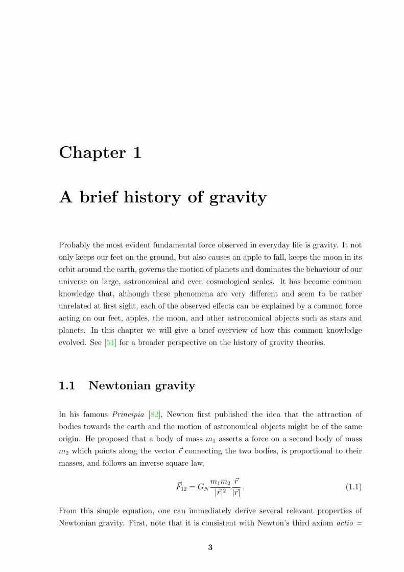
In his famous Principia [82], Newton first published the idea that the attraction of
bodies towards the earth and the motion of astronomical objects might be of the same
origin. He proposed that a body of mass m1 asserts a force on a second body of mass
m2 which points along the vector ~r connecting the two bodies, is proportional to their
masses, and follows an inverse square law,
~F12 = GNm1m2
|~r|2~r
|~r|. (1.1)
From this simple equation, one can immediately derive several relevant properties of
Newtonian gravity. First, note that it is consistent with Newton’s third axiom actio =
3

4 A brief history of gravity
reactio, i.e., the forces the two bodies assert on each other are of the same strength and
opposite direction, ~F12 = −~F21. Second, the acceleration of a body under the influence
of gravity is independent of its mass, which agrees with Galilei’s observation that bodies
of different mass and composition fall within equal times when they are dropped from
the same height.
One may view Newton’s universal law of gravity as an early step towards a unified
description of nature by physical laws. The stage on which these physical laws were set
was also provided by Newton’s Principia, and is known as Newtonian mechanics. It is
based on the assumption of fixed, non-dynamic, absolute, Euclidean space and, corre-
spondingly, a fixed, non-dynamic, absolute time. The dynamics of Newtonian mechanics
is described by the trajectories of bodies within this rigid background structure which
are governed by Newton’s axioms of motion.
1.2 Einstein gravity
For more than two centuries Newton’s theories of mechanics and gravity were undis-
puted. They were in precise agreement with the observed motion of the planets within
the solar system, taking into account that this motion is affected not only by the solar
gravitational attraction, but also by the mutual attraction of the planets themselves,
which causes small deviations from the Keplerian elliptical orbits. The first such devi-
ation that could not be explained by Newtonian physics was discovered by Le Verrier
in the mid-19th century [123]. It turned out that the perihelion precession of mercury
deviates from its expected value, caused by the gravitation of the other planets, by a
value of 43” per century. However, it was not realized that this effect originates from new
physics. Instead one assumed that an undiscovered planet was responsible for mercury’s
additional perihelion precession.
With the upcoming 20th century, several new discoveries were made that led to a
revolution in physics. Maxwell computed the equations of electrodynamics and found
that electromagnetic waves propagate at constant velocity [75], but it was unclear with
respect to which frame of reference this velocity was to be measured. Based on Newton’s
concept of absolute space and time it was assumed that an absolute frame of reference
exists that is distinguished as the rest frame of an invisible medium, the so-called “ether”.
Several experiments attempted to prove the existence of the ether, most notably the
interferometer experiment performed by Michelson and Morley [76], but it turned out

A brief history of gravity 5
that the speed of light is completely independent of any frame of reference.
The observed constant speed of light was first explained by Lorentz [70]. He sug-
gested that moving bodies contract, and moving clocks measure an amount of time
different from that measured by clocks at rest. These effects were summarized in a set
of transformation laws that allow to transform length and time measured within one
frame of reference into any other frame of reference. However, Lorentz still assumed the
existence of a Newtonian frame of reference with respect to which velocities should be
measured. This assumption was dropped by Einstein with the advent of special rela-
tivity [32]. His principle of relativity states that there is no distinguished, Newtonian
frame of reference, given by an absolute time and absolute space. Instead, all inertial
frames of reference, i.e., those with a constant relative velocity, are equivalent not only
within electrodynamics, but completely indistinguishable by any possible experiment.
A crucial consequence of Einstein’s theory is the relativity of simultaneity. Given any
two events and a frame of reference in which these events are simultaneous, there exist
further frames of reference, in which either of the events precedes the other one. If one
assumes that these events are causally connected, one easily arrives at a contradiction. If
each of the events precedes the other one in an appropriate frame of reference, there is no
possibility to distinguish which of the events causes the other one. This contradiction can
be resolved only if one assumes that there are no causal connections between events which
are simultaneous in an appropriate frame of reference. This turns out to be equivalent
to the statement that there is a maximum velocity for any information transfer which is
given by the speed of light.
Recall that within Newton’s theory of gravity, the gravitational force acting on each
body is determined by the positions of all gravitational sources at the same time, i.e., the
force changes instantaneously if a gravitational source at arbitrary distance changes its
position. This clearly contradicts the aforementioned consequence of special relativity
that an instantaneous transfer of information is not possible. Einstein soon realized that
a completely relativistic theory of mechanics would also require a new gravity theory
which takes into account that no signal travels at a higher velocity than the speed of
light.
An important step towards Einstein’s gravity theory is the weak equivalence princi-
ple: from the fact that the force acting on a massive body in a gravitational field and the
fictitious force acting on the same body in an accelerating frame of reference are identi-
cal, Einstein concluded that there is no principal distinction between a non-accelerating

6 A brief history of gravity
frame of reference with a gravitational field and an accelerating frame of reference with-
out a gravitational field [33]. From this conclusion, Einstein further deduced that the
light of a star should be red-shifted as it is passing through its gravitational field, and
that light should bend under the influence of gravity [34]. Einstein tried to formulate his
gravity theory in purely geometric terms. This led him towards the principle of general
covariance, i.e., the invariance of physical laws under general coordinate transformations,
or diffeomorphisms. Although he temporarily abandoned this principle, it was the key
idea that finally led him to the discovery of his famous field equations in 1915 [35].
An immediate success of Einsteins theory was the correct description of the perihelion
precession of mercury. However, general relativity gained a lot more popularity when
the prediction of the deflection of light was confirmed during the 1919 solar eclipse by
Eddington [31].
Although Einstein’s theory is still the most successful and accurate theory of gravity,
it has several problems. Modern astronomical observations have led to the discovery of
phenomena that cannot be explained completely within general relativity without the
proposal of new, hidden types of matter. Furthermore, it has turned out that there are
fundamental difficulties for the unification of general relativity and quantum theory - the
most important ingredient of modern physics, besides general relativity. We will examine
these problems in chapter 3, after providing a brief introduction into its mathematical
ingredients in the following chapter 2.

Chapter 2
Foundations of general relativity
In the previous chapter we have given a brief overview over the history of gravity, and
will now turn our focus to Einstein gravity. Here and in the following chapters, we
use the names “general relativity” and “Einstein gravity” interchangeably. We will start
with a brief overview over the mathematical preliminaries that are necessary to formulate
Einstein’s theory. We will then define the vacuum theory in terms of the Einstein-Hilbert
action and derive the vacuum field equations. Finally, we will show how matter couples
to gravity and display the combined equations of motion. Within the limits of this thesis,
we have to restrict ourselves to a very basic overview. A comprehensive introduction to
general relativity can be found in various textbooks such as [125] or [79].
2.1 Pseudo-Riemannian geometry
This section is intended to provide an introduction into the most important mathematical
ingredient of general relativity, which is pseudo-Riemannian geometry. We will only
sketch the basic definitions and theorems necessary for this thesis, and omit all proofs
and lengthy derivations. For a comprehensive introduction, see [109] or [81].
2.1.1 Manifolds and tensors
We start with the most basic object of pseudo-Riemannian geometry. A smooth manifold
of dimension n is a topological space M , together with an open cover (Ui, i ∈ I) and
7

8 Foundations of general relativity
homeomorphisms φi : Ui → Rn, such that for all i, j ∈ I the transition function
φji = φj ◦ φ−1i : φi(Ui ∩ Uj)→ φj(Ui ∩ Uj) (2.1)
is of class C∞. For simplicity we only consider smooth manifolds where the transition
functions are of class C∞, but we remark that the more general notions of differentiable
and topological manifolds exist where the transition functions are of class Ck or C0,
respectively.
In order to define vector and tensor fields on manifolds, we first consider maps be-
tween manifolds. A map f : M →M ′ between two manifolds M and M ′ is smooth, if for
each x ∈M there exist open sets x ∈ Ui ⊂M and f(x) ∈ U ′i′ ⊂M ′, such that φ′i′ ◦f ◦φ−1i
is smooth. We denote the set of smooth maps from M to M ′ by C∞(M,M ′). Two special
cases are of particular relevance. First, choosing M = R leads to the set C∞(R,M ′) of
smooth curves on M ′. Second, choosing M ′ = R gives us the set C∞(M,R) of smooth,
real-valued functions on M .
Let γ ∈ C∞(R,M) be a smooth curve on a manifold M . The tangent vector γp in
p = γ(0) ∈M is the map
γp : C∞(M,R) → R
f 7→ ddt
(f ◦ γ)(t)∣∣t=0
. (2.2)
For any given point p ∈M , the set of all tangent vectors γp associated to curves γ with
γ(0) = p forms an n-dimensional vector space, called the tangent space TpM of M at p.
Its dual is called the cotangent space T ∗pM . These spaces are the building blocks of the
tangent and cotangent bundles, which we will define shortly, and which are examples of
the following general construction:
A (smooth) fiber bundle (E,B, F, π) is constituted by three (smooth) manifolds, the
total space E, the base space B and the fiber F , and a (smooth) surjection π : E → B,
called its projection, such that for all x ∈ B there exists an open neighborhood U 3 xand a (smooth) homeomorphism h : π−1(U) → U × F so that the following diagram
commutes:
π−1(U)h //
π
��
U × F
p1
yysssssssssss
U
. (2.3)

Foundations of general relativity 9
Here, p1 denotes the projection onto the first factor U . It is common to simply denote
a fiber bundle by its total space E when the other constituents are clear. A section of
the bundle is a map s : B → E so that π ◦ s is the identity map on B. The space of all
sections is denoted Γ(E,B, F, π).
The union of all tangent spaces of a smooth manifold M forms the total space of
a smooth fiber bundle called the tangent bundle TM . Its base space is the manifold
M . Its fiber is an n-dimensional vector space isomorphic to the tangent space TpM at
an arbitrary point p ∈ M . The projection π maps each tangent vector γp to its base
point p. In complete analogy to this definition, the cotangent bundle T ∗M is the union
of all cotangent spaces of a smooth manifold M . Furthermore, the tensor bundle (TM)rs
for r, s ∈ N fixed is the union over all p ∈M of the tensor products
(TpM)rs = TpM ⊗ . . .⊗ TpM︸ ︷︷ ︸r factors
⊗T ∗pM ⊗ . . .⊗ T ∗pM︸ ︷︷ ︸s factors
. (2.4)
The tangent and cotangent bundles are reobtained as the special cases TM = (TM)10
and T ∗M = (TM)01.
An ordered basis of the tangent space TpM is called a frame at p. The space of
all frames at a given point p of a manifold M is not a vector space; it is, however, a
manifold. The union of these spaces is called the frame bundle GL(M). As the name
already suggests, the frame bundle is a fiber bundle and its base space is the manifold
M . The coframe bundle is defined in complete analogy.
Smooth sections of the tensor bundle (TM)rs are called (r, s)-tensor fields. Smooth
sections of the tangent and cotangent bundles are called vector and covector fields, re-
spectively. Finally, smooth sections of the (co)frame bundle are called (co)frame fields.
A particular class of frame fields can be obtained from a coordinate representation:
Let M be a manifold and U ⊂M some open neighborhood that is parametrized by a set
of coordinates xa, a = 1, . . . , n. For each point p ≡ xa ∈ U , there is a set of coordinate
curves γb : t 7→ xa + tδab , b = 1, . . . , n passing through p at t = 0. The tangent vectors
∂b(p) = (γb)p form an ordered basis of the tangent space TpM and thus define a frame
field ∂b. The dual basis of ∂b(p) is a basis dxb(p) of the cotangent space T ∗pM , and defines
a coframe field dxb.
Frames and coframes provide a convenient way to express tensor fields. Let (ea(p) ∈TpM,a = 1, . . . , n) be an ordered basis of TpM , and (θa(p) ∈ T ∗pM,a = 1, . . . , n) dual

10 Foundations of general relativity
basis of T ∗pM . An ordered basis of the tensor product space (TpM)rs is then given by
ea1(p)⊗ . . .⊗ ear(p)⊗ θb1(p)⊗ . . .⊗ θbs(p) . (2.5)
A section of the frame bundle provides us with such a basis at each point of the manifold
and allows us to expand a tensor field X ∈ Γ((TM)rs) in the form
X = Xa1...arb1...bsea1 ⊗ . . .⊗ ear ⊗ θb1 ⊗ . . .⊗ θbs , (2.6)
where the tensor components X = Xa1...arb1...bs now are real-valued functions on M .
Tensors are commonly written in terms of their components with respect to some basis.
Here and in the remaining chapters of this thesis we use the Einstein summation con-
vention: If a tensor index appears both in upper and lower position, it is understood as
a sum,
Xa1...c...arb1...c...bs ≡
n∑c=1
Xa1...c...arb1...c...bs . (2.7)
In the following sections, we will use these very basic objects of differential geometry
to define the metric, the connection and the curvature of a pseudo-Riemannian manifold.
2.1.2 The metric tensor
The smooth manifold structure we have defined in the previous section provides a notion
of smooth functions and smooth curves. However, it does not allow to measure the length
of a curve. Neither does it allow to measure the intersection angle between intersecting
curves. In this section, we add the missing structure that allows for the measurement of
lengths and angles. This structure is called the metric.
Let M be a smooth manifold. A metric g is a non-degenerate, symmetric (0, 2)-tensor
field on M . This means that the components of the metric satisfy the relation gab = gba
and a (2, 0)-tensor field g−1 exists such that gabgbc = δac .
An important property of the metric is its signature. According to Sylvester’s theo-
rem, it is possible to choose a basis of the tangent space TpM at each point p ∈ M so

Foundations of general relativity 11
that the metric takes the form
gab =
−1k 0
0 1l
= η(k,l)ab , (2.8)
where 1k denotes a unit matrix of dimension k and k + l = n is the dimension of M . A
basis of this type is called an orthonormal frame. Since the metric depends smoothly on
the spacetime point p, the numbers (k, l) are constants. These are called the signature
of the metric manifold (M, g). In the special cases k = 0 and k = 1, the metric is called
Riemannian or Lorentzian, respectively.
Let (M, g) be a Lorentzian manifold and v ∈ TpM a vector at some point p ∈ M . v
is called timelike if gabvavb < 0; lightlike or null if gabv
avb = 0; spacelike if gabvavb > 0.
Smooth curves on M are called timelike, lightlike or spacelike, if their tangent vectors
at every point of the curve have this property. In the following, we will consider only
curves which are either spacelike or timelike.
Let γ ∈ C∞([a, b],M) be a smooth curve defined on the interval [a, b]. Its length s is
given by
s =
∫ds =
∫ b
a
dt√|gab(γ(t))γa(t)γb(t)| (2.9)
as the integral over the line element ds,
ds2 = |gab(γ(t))γa(t)γb(t)|dt2 . (2.10)
A curve of extremal length between two given endpoints is called a geodesic. Besides
providing a length measure, the metric also defines a measure for angles. Let γ, γ′ ∈C∞(R,M) be two smooth curves intersecting in p = γ(0) = γ′(0). Their intersection
angle α is given by√|gab(γ(0))γa(0)γb(0)|
√|gab(γ′(0))γ′a(0)γ′b(0)| cosα = gab(γ(0))γa(0)γ′b(0) . (2.11)
Furthermore, the metric provides a measure for areas. An infinitesimal area element
can be viewed as a parallelogram spanned by two vectors v, w at the same point p. Its
squared area is given by
gab(p)vavbgcd(p)w
cwd − (gab(p)vawb)2 . (2.12)

12 Foundations of general relativity
Finally, the metric (and its inverse) are used to lower and raise indices, i.e., as a map
from the tangent to the cotangent bundle and vice versa,
va = gabvb, va = gabvb . (2.13)
2.1.3 Parallel transport and Levi-Civita connection
In section 2.1.1 we defined the tangent bundle of a smooth manifold as the union of
the individual tangent spaces at each point. Since these are isomorphic, but different
vector spaces, there is no a priori possibility to compare elements of one tangent space
to elements of another. We will now introduce a structure that adds this possibility.
This structure is called a connection.
We start with the notion of parallel transport. For simplicity, we restrict ourselves
to the following setting. Let p ∈ M be a point and v ∈ TpM a vector at p. We wish
to parallely transport v to a point p′ close to p, such that p and p′ are connected by a
vector field X. This means that in an appropriate coordinate system, the coordinates
of p and p′ are related by p′a = pa + Xa and the components Xa are small enough to
approximate the parallely transported vector v′ ∈ Tp′M in the form
v′a = va − ΓabcvbXc , (2.14)
where we omitted all terms beyond the linear order in X. The coefficients Γabc in this
expansion are called the connection coefficients, or Christoffel symbols.
We can now generalize this infinitesimal parallel transport to the parallel transport
along an integral curve of X, i.e., a curve γ ∈ C∞(R,M) so that its tangent vector γ(t)
at p = γ(t) equals X(p). From equation (2.14) one can read off the condition
va = −ΓabcvbXc , (2.15)
where va denotes the derivative of the component va with respect to the curve param-
eter t. We can further generalize the concept of parallel transport. Let X, V be vector
fields. V is parallely transported along X, if it is parallely transported along every inte-
gral curve of X. Using the definition of the integral curve, we can rewrite the derivative

Foundations of general relativity 13
of the component V a as
d
dtV a(γ(t)) = Xc(γ(t))∂cV
a(γ(t)) , (2.16)
and finally obtain the condition
0 = (∇XV )a = Xc∂cVa + ΓabcV
bXc . (2.17)
The vector field ∇XV is called the covariant derivative of V with respect to X.
In the case that a vector field X is parallely transported along itself, ∇XX = 0, X
is called an autoparallel vector field. Its integral curves γ are called autoparallels and
satisfy the equation
γa + Γabcγbγc = 0 . (2.18)
The covariant derivative can be generalized further to operate on arbitrary tensor
fields. Let X be a vector field and T be a (r, s)-tensor field. The covariant derivative of
T with respect to X can be written in the form
(∇XT )a1...arb1...bs = Xd∂dT
a1...arb1...bs +
r∑i=1
ΓaicdT
a1...c...arb1...bsX
d
−s∑i=1
ΓcbidTa1...ar
b1...c...bsXd .
(2.19)
We now have two different structures defined on the manifold: the metric and the
connection. The question arises whether these two structures can be related. This is
indeed possible. It turns out that there exists a unique connection so that the Christoffel
symbols are symmetric in their lower pair of indices (which corresponds to vanishing
torsion) and the covariant derivative of the metric vanishes. This connection is called
the Levi-Civita connection, and its components take the form
Γabc =1
2gad(∂bgcd + ∂cgbd − ∂dgbc) . (2.20)
The Levi-Civita connection has the remarkable property that its autoparallels are pre-
cisely the geodesics of the metric.

14 Foundations of general relativity
2.1.4 Riemann curvature
In the preceding section we have shown that vectors on a manifold equipped with a
connection can be parallely transported along a curve. We will now consider the special
case that a vector is parallely transported along a closed curve. Let p = γ(0) = γ(1) ∈Mbe the common start and end point of a curve γ ∈ C∞(R,M). Parallel transport along
γ then defines an endomorphism of the tangent space TpM . One may now ask under
which conditions this endomorphism is the identity map.
We first reformulate the question and ask: Under which conditions is the parallel
transport from a point p to a point q independent of the curve connecting p and q?
In order to answer this question, we consider the case that p and q are infinitesimally
close to each other. We further choose two additional points p′, q′ close to p, q and two
coordinate vector fields X, Y with [X, Y ] = 0 connecting the points as shown in the
following diagram:
q′X // q
pX//
Y
OO
p′
Y
OO
A vector v ∈ TpM can now be parallely transported either from p to p′ along X and then
to q along Y , or from p to q′ along Y and then to q along X. The difference between
the two resulting vectors at q is given by
δv = ∇X∇Y v −∇Y∇Xv . (2.21)
In tensor components, this takes the form
δvi = Rijklv
jXkY l , (2.22)
where we introduced components of the Riemann curvature tensor
Rijkl = ∂kΓ
ijl − ∂lΓijk + ΓikpΓ
pjl − ΓilpΓ
pjk . (2.23)
We can now answer the question posed at the beginning of this section: The parallel
transport of a vector is independent of the curve if and only if the Riemann curvature
tensor vanishes.

Foundations of general relativity 15
From the Riemann tensor one further derives the Ricci tensor
Rij = Rpipj (2.24)
and the Ricci scalar
R = gijRij , (2.25)
which will become important in the following sections.
2.2 Einstein-Hilbert action
In the previous section 2.1 we presented the mathematical foundations necessary to
formulate Einstein’s gravity theory. We will now use these definitions and present a
short overview of general relativity. In this section, we start by introducing the Einstein-
Hilbert action, from which we derive the vacuum field equations. The coupling between
matter fields and gravity will be discussed in the next section 2.3.
Probably the simplest and shortest approach towards the field equations of general
relativity is to start from the Einstein-Hilbert action,
SG =1
16πGN
∫M
ωR , (2.26)
where GN denotes the Newton constant introduced in equation (1.1), M is the spacetime
manifold equipped with a Lorentzian metric g of signature (1, 3), and ω = d4x√g is the
volume form. The field equations can be obtained by variation of this action with respect
to the metric gab. First, we compute the variation of the volume form,
δω =1
2d4x√g gabδgab =
1
2ωgabδgab . (2.27)
We then compute the variation of the Ricci scalar R = gijRij. This can be split into
two terms: the variation of the inverse metric reads
δgij = −giagbjδgab , (2.28)

16 Foundations of general relativity
while the variation of the Ricci tensor can be written in the form
δRij = ∇k(δΓkij)−∇i(δΓ
kjk) . (2.29)
This combines to the variation of the Ricci scalar,
δR = −giagbjRijδgab +∇k(gijδΓkij)−∇i(g
ijδΓkjk) , (2.30)
where we used the fact that the metric, and thus also its inverse, is covariantly constant,
∇kgij = 0. The last two terms are total derivatives, and thus can be omitted from the
variation of the action. The total variation finally reads
δSG =1
16πGN
∫M
ω
(1
2gabR−Rab
)δgab . (2.31)
We can thus read off the Einstein field equations in vacuum:
Rab − 1
2gabR = 0 . (2.32)
2.3 Matter and energy-momentum tensor
In the previous section, we derived the gravitational vacuum field equations by variation
of the Einstein-Hilbert action. Of course any theory of gravitation is completely specified
only after matter coupling; this will be provided in this section. For this purpose, we
add an additional term
SM =
∫M
ωLM (2.33)
to the action, where the scalar LM denotes the matter Lagrangian. We do not specify
the exact form of LM as it is not relevant for the calculations in this section, but one
may think of LM as being the standard model Lagrangian. The variation of the matter
action with respect to the metric takes the form
δSM =1
2
∫M
ωT abδgab , (2.34)

Foundations of general relativity 17
where we have introduced the energy-momentum tensor
T ab =2√−g
δ(LM√−g)
δgab. (2.35)
The complete gravitational equations of motion, obtained from the variation of the full
action S = SG + SM , finally read
Rab − 1
2Rgab = 8πGNT
ab . (2.36)
This is the general form of the Einstein equations [35]. Variations of 2.33 with respect to
the matter fields provide the matter field equations on the curved spacetime background.

18

Chapter 3
Problems of general relativity
Up to now we have given two different introductions to general relativity: a historic
introduction in chapter 1 and a mathematical introduction in chapter 2. We have pre-
sented general relativity as a theory both of mathematical beauty and physical accuracy
for explaining astronomical observations both within and beyond our solar system. If
this was already the end of the story, we could stop at this point and leave general
relativity as it is. However, nature is not that simple. General relativity poses several
questions which we will examine in detail in this chapter. First, we will discuss astro-
nomical observations that cannot be explained completely by the assumption of purely
visible gravitational sources whose dynamics is governed by general relativity. In order
to explain these observations, either a modified gravity theory, or additional dark sources
of gravity are required. Second, we will turn our focus to theoretical complications that
arise from the interplay between the most important ingredients of modern theoretical
physics, namely general relativity and quantum theory.
3.1 Astronomical observations
General relativity provides explanations for various astronomical observations, most no-
tably the perihelion precession of mercury and the deflection of light by the solar grav-
itational field. However, in the last 80 years several observations have been made that
cannot be explained by general relativity alone. In this section we will give a brief
overview of such observations and how the observed effects are conventionally explained
by additional matter sources or modified gravity theories.
19

20 Problems of general relativity
3.1.1 Peculiar velocities in galaxy clusters
The first hint on new physics comes from the observation of galaxies in the Coma clus-
ter. Measurements of their peculiar velocities and visible masses have shown that the
virial theorem, which is a consequence of the Newtonian limit of general relativity, is
apparently violated [135]. This observation led to the conclusion that the masses of the
galaxies are in fact significantly higher that their visible masses obtained from lumi-
nosity measurements. Since the additional mass does not emit any detectable form of
radiation, and thus appears dark, is has become popular under the name dark matter.
3.1.2 Gravitational lensing
In section 1.2 we mentioned the deflection of electromagnetic waves by massive objects
as one of the first and most successful predictions of general relativity. High precision
measurements of the deflection of light and radio waves within the gravitational fields of
the sun and Jupiter [107, 117] and the time delay due to the larger length of the actual
path [98] have quantitatively confirmed this prediction within very narrow bounds. One
might thus expect that observations of light deflection by more massive objects, such as
galaxies or galactic clusters, should also agree with Einstein’s prediction.
There are numerous examples of objects for which light deflection has been ob-
served [126]. However, the measured deflection angles are significantly larger than one
might expect by estimating the mass of the gravitating object from its visible con-
stituents. This is another hint that the total mass of the galaxies receives an additional
contribution from dark matter.
3.1.3 Rotation curves of galaxies
A further hint for the existence of dark matter comes from the observed rotation curves
of galaxies. If the motion of galactic matter constituents, i.e., stars and interstellar gas,
around the galactic center was governed only by the Newtonian potential of a central
point mass, their velocity should decrease with increasing distance from the galactic
center according to Kepler’s third law.
However, observations show that the velocity of the galactic matter constituents
is almost independent of their distance from the galactic center [14]. This could be

Problems of general relativity 21
explained by the presence of additional dark gravity sources distributed along with the
visible matter. Other potential explanations include modified Newtonian dynamics [77]
and general relativistic effects beyond the Newtonian limit [27].
3.1.4 Structure formation
Observations of the cosmic microwave background have shown that the matter distri-
bution in the early universe was nearly homogeneous, with very small density fluctua-
tions [64]. This significantly differs from the present state of the universe where visible
matter appears to be organized hierarchically: stars form galaxies, galaxies form galactic
clusters and superclusters and superclusters form a filament-like structure around huge,
nearly empty voids [25, 1].
If one assumes that visible matter is the only matter constituent of the universe and
that the small density fluctuations have evolved to the present large-scale structure one
arrives at a problem: The initial density fluctuations in the early universe are too small
to explain the observed large-scale structure [88].
As it was already the case in the preceding sections, dark matter provides a poten-
tial solution to this problem. An additional, dark type of matter that interacts only
gravitationally could have decoupled from the hot baryonic matter content of the early
universe, and thus formed structures prior to the structure formation of visible matter.
These dark structures might then have attracted the visible matter and led to the for-
mation of the visible large-scale structure [15]. This explanation is supported by recent
simulations of structure formation [111]. However, it is only valid for cold, non-baryonic
dark matter whose constituents are presently unknown.
3.1.5 Accelerating expansion of the universe
One of the first exact solutions of the Einstein equations has been constructed indepen-
dently by Friedmann [39] and Lemaıtre [69]. They started from the assumption that the
universe is homogeneous and isotropic, and that its matter content is constituted by a
perfect fluid of either dust or radiation. This simple cosmological model led to a clear
and unexpected prediction: it turned out that the universe should either collapse within
a finite time, or expand, starting from an initial singularity. This prediction contradicted
the widely accepted model of a static universe. Einstein was very unhappy with this pre-

22 Problems of general relativity
diction and modified his field equations by introducing a “cosmological” constant Λ into
the action of general relativity in order to obtain static cosmological solutions. However,
Hubble [59] discovered a correlation between the distance of galaxies and their velocity
with respect to our galaxy, measured by the Doppler red-shift. This observation strongly
supported a uniformly expanding Friedmann-Lemaıtre universe. When Einstein became
aware of this observation, he dropped the cosmological constant from his theory, calling
it his “biggest blunder” [40].
Modern observations, however, suggest that Einstein’s cosmological constant might
deserve a revival. According to the Friedmann-Lemaıtre model, the expansion of the
universe should decelerate due to the mutual attraction of its matter content. Precise
measurements of the Doppler red-shift of type Ia supernovae in distant galaxies have
shown that the opposite is true and the expansion of the universe is in fact acceler-
ating [100, 90]. This observation cannot be explained within the Friedmann-Lemaıtre
model of a universe filled with dust or radiation, or a combination of visible and dark
matter, without a cosmological constant.
In the widely accepted standard model of cosmology, the so-called ΛCDM model,
the cosmological constant is modelled as another obscure type of matter, denoted “dark
energy” [61]. Within this model, only 4.6% of the total matter content of the universe
is constituted by visible matter; the remaining 95.4% are 22.8% dark matter and 72.6%
dark energy [64]. However, the constituents of dark energy are presently unknown.
3.1.6 Galaxies in the vicinity of voids
In the preceding section 3.1.5 we have discussed the dynamics of the universe on very
large, cosmological scales, which enabled us to assume that the universe is homogeneous
and isotropic. We will now turn our view back to the supergalactic scale of clusters and
voids discussed in section 3.1.4. Our galaxy belongs to a structure known as the Local
Sheet which is located in the vicinity of a large void, correspondingly known as the Local
Void. Measurements of the peculiar motion of our neighboring galaxies have shown that
the overall velocity of the Local Sheet relative to surrounding supergalactic structures is
large compared to relative velocities of individual galaxies. This large relative velocity
which separates the Local Sheet from other structures in our vicinity is known as the
local velocity anomaly [118, 119, 120].
A closer look at the motion of the Local Sheet shows that its velocity can be decom-

Problems of general relativity 23
posed into three components, two of which can be explained by the attraction towards
the Virgo and Centaurus galactic clusters. The remaining component is not directed
towards any visible structure; it is, however, directed away from the Local Void. This
suggests that the Local Void expands, and thus pushes the Local Sheet away from its
center, and is conventionally explained by the absence of any type of matter besides
dark energy in very large region.
3.1.7 Pioneer anomaly
The astronomical observations we have discussed so far have in common that they are
relevant only on very large scales, comparable at least to the size of our galaxy. Neverthe-
less, possible evidence for a deviation from general relativity exists also within our solar
system. The most important example of such evidence is the Pioneer anomaly [121],
which was named after the space probes Pioneer 10 and Pioneer 11 launched in 1972
and 1973. It denotes the observed deviation of the trajectories of various unmanned
spacecrafts in the solar system from their expected trajectories due to the combined
gravitational effects of the sun and the planets. This deviation can be accounted for by
a constant force directed towards the sun, causing the spacecraft to decelerate on their
way through the outer solar system.
Various possible explanations for the observed anomalous deceleration have been
proposed, including measurement errors, thrust from gas leakage, anisotropic thermal
radiation, and the drag of the interplanetary medium. Besides these rather conventional
explanations, the Pioneer anomaly has also stimulated the development of new physical
theories, such as modified Newtonian dynamics, clock acceleration, light acceleration, or
a violation of the weak equivalence principle. However, it is still unknown which, if any,
of these effects is responsible for the Pioneer anomaly.
3.2 Quantization
In the preceding section 3.1 we have discussed open questions of general relativity that
arise from astronomical observations. But there are also theoretical problems arising
from the interplay between general relativity and quantum theory. We will now discuss
these problems and give some hints on possible solutions.

24 Problems of general relativity
3.2.1 Necessity of a quantum theory of gravity
Both general relativity and quantum theory have been confirmed experimentally with
high precision within their respective ranges of validity. General relativity provides
an accurate description for large-scale gravitational effects, while quantum theory accu-
rately describes small-scale effects occurring in the physics of atoms, nuclei or elementary
particles. However, one may easily think of physical situations in which both theories
must be considered.
One of the most prominent consequences of general relativity is that matter that is
compressed into a sufficiently small radius inevitably collapses and forms a black hole,
and that it must be surrounded by an event horizon which does not allow matter or
information to leave the black hole. This is summarized by the no-hair theorem [104],
which states that for an exterior observer a black hole is completely characterized by
its mass, angular momentum and electric charge. Quantum theory further requires
that black holes must have an entropy related to their mass, and must emit thermal
radiation [50], which is completely random due to the no-hair theorem. From the energy
loss due to thermal radiation it then follows that black holes must evaporate in finite
time. From the randomness of the thermal radiation it follows that all information
thrown into a black hole is lost. Quantum theory, however, states that the evolution of
any physical system must be unitary and thus information cannot be destroyed. This
contradiction is known as the black hole information paradox.
Of course the presence of such paradoxa in the framework of modern physics is
an utterly dissatisfying situation, and one is led to the question whether both general
relativity and quantum theory arise as appropriate limits on an underlying, fundamental
theory, which resolves these problems. Unfortunately the construction of such a unified
theory poses various problems, a few of which we will discuss in the following.
3.2.2 Problems of quantization
Quantum theories such as quantum mechanics or quantum field theory are formulated on
the fixed, non-dynamic background structure of Minkowski spacetime or, more generally,
a globally hyperbolic spacetime. In general relativity, however, an a priori geometric
structure does not exist. It is the geometry of spacetime itself that is the dynamical
variable of the theory. This raises the question how a theory can be quantized without
assuming such an a priori structure. This is known as the problem of background-

Problems of general relativity 25
independence.
Another obstacle to the quantization of gravity is its non-renormalizibility. If one
assumes that the gravitational field can be considered as a perturbation around the flat
Minkowski metric and directly quantizes this field, one obtains divergences that cannot
be resolved using the standard method of renormalization. A perturbative approach
towards quantum gravity, in analogy to other quantum field theories, thus is not possible.
3.2.3 Possible solutions
We have seen that the construction of a quantum theory of gravity is obstructed by
various difficulties. We will now briefly discuss the most prominent candidate theories
for quantum gravity, and how these difficulties might be resolved.
String theory
Although string theory has been developed originally as a model for the strong inter-
action [122], it has become one of the most promising candidates for a unified theory
of all fundamental forces, including gravity. Its basic ingredient of is the replacement
of point particles by one-dimensional, extended objects, called strings. The motion of
classical strings is governed by their tension and kinetic energy, so that they behave
as harmonic oscillators. The quantization of these oscillators then leads to an infinite
tower of string states, which are interpreted as particle spectra. These spectra naturally
feature a massless spin two field, which in turn is interpreted as the graviton [46, 91].
Although string theory has become very popular as a theory of high mathematical
elegance, it has several problems. The most obvious is the prediction of six additional,
presently unobserved dimensions of spacetime. It is commonly assumed that these extra
dimensions are “compactified” at a scale comparable to the Planck scale and can thus
only be probed by energies far beyond any possible accelerator experiment. Another
problem of string theory is the vast number of over 10500 string vacua that correspond
to universes with four dimensions, a high Planck scale, gauge groups and chiral fermions,
and the infinite number of vacua for different universes. At present it is unknown whether
it is the consequence of any underlying principle which of these vacua is realized in nature.

26 Problems of general relativity
Loop quantum gravity
A completely different approach to a quantum theory of gravity is loop quantum grav-
ity [114, 102]. Its basic ingredient is the reformulation of the metric in terms of Ashtekar
variables [5]. These variables can be quantized by a method known as loop quantization.
The resulting quantum theory leads to a replacement of the continuum of space by a
discrete, network-like structure. Each state of this so-called spin network represents a
possible spatial geometry. The evolution of these geometries is modelled by discrete time
steps.
One of the major successes loop quantum gravity claims is the resolution of the big
bang singularity. By the introduction of a fundamental length scale, the singularity is
avoided in favor of a big bounce when the cosmological scale factor comes close to the
minimal length. Another consequence of the construction of loop quantum gravity is its
background-independence, since the formalism does not assume an a priori geometric
structure, it does not even require the presence of a manifold structure. However, this
is also the most important problem of loop quantum gravity: it lacks the re-emergence
of a classical spacetime manifold from states of the spin network.

Chapter 4
Outline of the thesis
The aim of this thesis is to examine two different geometric theories which address some
of the problems of general relativity we mentioned in chapter 3. The thesis is divided
into two parts:
In part I we deal with multimetric gravity theories containing N > 1 copies of
standard model matter, each of which is governed by its own metric tensor. These
theories are constructed so that the interaction between the different standard model
copies, or sectors, is purely gravitational. This means that matter from one sector
appears dark to observers residing in a different sector. To be more specific, we will focus
on theories in which the gravitational interaction between the different types of matter
is repulsive and of equal strength compared to the attractive gravitational interaction
within each sector. We argue that theories of this type might explain the observed
accelerating expansion of the universe mentioned in section 3.1.5 by the mutual repulsion
of galaxies within different sectors. They might further provide a possible explanation
for the local velocity anomaly mentioned in section 3.1.6 under the assumption that
galaxies in the Local Sheet are accelerated in the gravitational field generated by a
repulsive gravity source in the Local Void.
We will start with an introduction in chapter 5 and argue why the incorporation
of repulsive gravity into general relativity naturally leads to multimetric gravity. We
will briefly explain how this might explain the observed accelerating expansion of the
universe and the local velocity anomaly, and how theories of this type may be tested.
In chapter 6 we will then examine the simplest type of multimetric theories, which is
the bimetric case N = 2. We will prove a no-go theorem which rules out the possibility
27

28 Outline of the thesis
of gravitational forces of equal strength and opposite direction acting on the two classes
of test masses in bimetric gravity theories. In chapter 7 we will show that this theorem
cannot be extended beyond the bimetric case by explicitly constructing a multimetric
repulsive gravity theory containing N ≥ 3 sectors. We will study this theory in the
following chapters. In chapter 8 we will construct a simple cosmological model for a
homogeneous and isotropic universe. We will show that our theory indeed leads to the
desired accelerating expansion, and that the acceleration naturally becomes small for
late times. In chapter 9 we will derive a simple model for structure formation from
the cosmological dynamics and the Newtonian limit of our theory. Starting from a
homogeneous matter distribution, we will simulate the evolution of small perturbations
using methods from computational physics. It will turn out that already this simple
model leads to the formation of filament-like structures for each matter type, surrounding
large voids which appear empty to observers within the same sector. These voids are
not empty as in standard cosmology, but instead contain matter from different sectors
and thus act repulsively on visible matter. In chapter 10 we will discuss the consistency
of our multimetric gravity theory with solar systems experiments. For this purpose
we will construct an extension of the parametrized post-Newtonian (PPN) formalism
to multimetric gravity and apply this extended formalism to our theory. It will turn
out that the PPN parameters of our theory do not match the observed values, but this
can be fixed by adding simple correction terms to the gravitational part of the action
without changing the dynamics of cosmology or structure formation. We conclude with
a discussion in chapter 11.
In part II we will turn our focus to the problem of quantization detailed in section 3.2.
We will present a mathematical framework which unifies the concepts of differentiable
manifolds and function spaces, which are the most basic mathematical ingredients of
general relativity and quantum theory. We will argue that a complete theory of quantum
gravity should reproduce both of these mathematical concepts in appropriate limits. We
will show that this is indeed true for our quantum manifold construction and present
some hints on possible physical interpretations.
In chapter 12 we will explain the basic idea of quantum manifolds and how this idea
is linked to the mathematical frameworks of differentiable manifolds and function spaces,
which are conventionally used to model gravity and quantum theory. In chapter 13 we
will review the basic mathematical ingredients of our construction. We will use these
ingredients to define a quantum manifold in chapter 14 and show that every quantum
manifold has a classical limit, which is simply an ordinary, differentiable manifold. In

Outline of the thesis 29
chapter 15 we will discuss further properties of quantum manifolds. We will show that
a quantum manifold is in fact a fiber bundle over its classical limit, and that every
ordinary differentiable manifold can be turned into a quantum manifold using the trivial
fiber bundle. This will conclude our mathematical construction. In chapter 16 we will
speculate on possible physical interpretations for our quantum manifold framework in
the contexts of quantum field theory and quantum mechanics. This part of the thesis
will be concluded with a discussion in chapter 17.
We will summarize our results at the end of this thesis and provide an outlook to
possible future research.
The main text of this thesis is supplemented by several appendices. Appendix A
lists the complete source code used for the simulation of structure formation described
in chapter 9. In appendix B we display the coefficients used in the linearized version
of the PPN formalism in section 10.3. Appendix C contains several technical proofs
required for the quantum manifold constructions in part II.
This thesis is further supplemented by various visualizations of the results from our
simulation of structure formation detailed in chapter 9. These include videos, three-
dimensional graphics, high-resolution images and Mathematica files. Please contact the
author for further information.
Parts of this thesis have been presented in several articles. The no-go theorem of
chapter 6 can be found in [54]. The multimetric gravity theory of chapter 7 and its
cosmology shown in chapter 8 are displayed in [55]. The multimetric extension to the
parametrized post-Newtonian formalism of chapter 10 and its application to our theory
are presented in [56]. The quantum manifold construction of part II is discussed in [53].

30

Part I
Multimetric repulsive gravity
31


Chapter 5
Introduction
In this part of the thesis we will examine theories containing N > 1 copies of standard
model matter, where the interaction between the different standard model copies is
purely gravitational and repulsive. The aim of this work is to address several of the
astronomical observations listed in section 3.1. Most notably, we will show that theories
of this type provide a potential explanation for the formation of filament-like structures
and voids (see section 3.1.4), the observed accelerating expansion of the universe (see
section 3.1.5) and the local velocity anomaly (see section 3.1.6).
This chapter contains a brief introduction to multimetric gravity theories. In sec-
tion 5.1 we will explain the role of mass in Newtonian gravity. We will see that the
positivity of mass is closely linked to the observational fact that gravity is always at-
tractive, and that repulsive gravitational forces can be modelled by the introduction of
negative masses. Taking the step from Newtonian to Einstein gravity, we will see that
the concept of negative mass naturally leads to multimetric theories in which the mo-
tion of each type of matter is governed by its own metric tensor. The physical relevance
of repulsive gravity is discussed in section 5.2. We will explain how this idea might
be used as a model for both dark matter and dark energy, and we will refer to some
of the astronomical observations listed in section 3.1 and give potential explanations
for these in the context of repulsive gravity. We will further discuss the advantages
of repulsive gravity as opposed to other models of dark matter and dark energy. Fi-
nally, in section 5.3 we will consider experimental tests of repulsive gravity. We will
show that multimetric repulsive gravity models can easily be tested with available high-
precision data from solar system experiments by employing an extended version of the
parametrized post-Newtonian formalism.
33

34 Introduction
5.1 Repulsive extension of general relativity
In Newtonian mechanics and gravity the notion of mass appears as a generic term in
quite different physical contexts. Taking a closer look one needs to distinguish three
different types of mass [19]: active gravitational mass ma is the source of gravitational
fields; passive gravitational mass mp determines the force acting on a test particle in
a gravitational field; inertial mass mi serves as the proportionality factor relating force
and acceleration.
Experiment, however, shows that these at first unrelated types of mass are closely tied
together. Both ratios ma/mp and mi/mp appear to be constant independent of material,
see e.g. [65, 9, 129] and [37, 101, 85, 132]. These observations are nicely explained by well-
known theoretical principles. Newton’s third law asserts that for every force there exists
a reciprocal force of equal strength and opposite direction. Considering the gravitational
force, this implies that the ratio ma/mp between active and passive gravitational mass
must be equal for all bodies. The weak equivalence principle states that the acceleration
of a physical body in a gravitational field is independent of its composition. This implies
that the ratio mi/mp between inertial and passive gravitational mass is fixed. It is
conventional to choose unit ratios so that all three masses become equal. Taking into
account the observational evidence that gravity is always attractive, all mass can be
chosen positive.
One may now argue that the experiments and observations mentioned above approve
the proportionality and positivity of the different types of mass only for visible matter,
i.e., for matter observed through non-gravitational interactions, say through emitted
light or other types of radiation. However, assuming Einstein gravity, modern astro-
nomical observations [64] suggest that visible matter only constitutes a small fraction
of about 5% of the total matter content of the universe. The main constituents of the
universe, known as dark matter and dark energy, have not been observed directly. So
it remains unknown whether the same fixed ratio relations between the different types
of mass are obeyed also in the dark universe. This lack of knowledge hence invites the
interesting possibility to modify Newton’s third law, the weak equivalence principle, or
the positivity of mass.
In this part of the thesis we will accept this invitation, and consider gravity theories
with a modified weak equivalence principle. We will investigate a different ratio between
inertial and passive gravitational mass in the dark sector, namely mi/mp = −1. Assum-

Introduction 35
ing that the inertial mass is still positive, we thus have mp = ma and |mp| = mi in both
sectors. This modification introduces negative gravitational masses in such a way that
like masses attract while unlike masses repel each other.
Neither the concept of negative mass nor its cosmological motivation are new in the
literature, and have been discussed within several theoretical contexts and with different
ratios and signs of ma, mp and mi. Already in 1897, Foppl [38] introduced negative mass
as a natural extension of Newtonian gravity. Consequences within modified Newtonian
dynamics have been discussed e.g. in [78]. It has been observed that additional negative
masses with ma = mp = mi < 0 neither violate Newton’s third law, nor the weak
equivalence principle. Forces on such bodies cause these to accelerate in the opposite
direction. Probably the most striking example for this behaviour is the gravitational
dipole: a system of two bodies of positive and negative mass must forever accelerate
in a common direction, the negative mass following the positive one. This effect also
exists within Einstein gravity [19, 41], where the ratio mi/mp = 1 is manifestly fixed
by the weak equivalence principle. Considering only gravitational forces, such that the
acceleration of a body is determined purely by the ratio mi/mp, the individual signs of
mp and mi do not affect the trajectories. Thus the only possibility to introduce negative
mass into Einstein gravity is to choose negative sources for the gravitational field, i.e.,
ma < 0. Various properties of such negative mass solutions have been discussed; for
instance, gravitational lensing [116], gravitational collapse [73] and the stability [42, 44]
of negative mass black holes. More general repulsive gravitational effects are analyzed
e.g. in [49, 74, 93].
A consequence of the weak equivalence principle is that all test masses, and all
observers, follow the same set of preferred curves, namely geodesics. In other words,
there is only one type of observers. Since we wish to relax this condition by allowing
the ratio mi/mp = −1 for a second type of matter, we have to extend the framework
of Einstein gravity. Indeed, it seems natural to introduce a second metric to generate
another set of geodesics describing the response of the negative mass observers to the
gravitational field. Only then can the gravitational force of a given source be attractive
for one class of test particles, while being repulsive for a second class. Such bimetric
theories with an antisymmetry between the forces acting on positive and negative masses
have become popular under the name ‘antigravity’ [57, 58], but their consistency, in
particular their diffeomorphism invariance, has been doubted [84].
Although bimetric gravity is the arguably simplest possible extension to general
relativity that allows both attractive and repulsive gravitational forces, one may easily

36 Introduction
generalize this idea to N > 2 types of matter, each of which is governed by its own
metric tensor, so that like masses attract while unlike masses repel each other in the
Newtonian limit. The idea of a repulsive extension to Einstein gravity thus naturally
leads to the concept of multimetric theories.
5.2 Repulsive gravity effects
We will now discuss how repulsive gravity might explain some of the astronomical ob-
servations we presented in section 3.1. We will mainly focus on cosmological aspects,
such as the cosmological structure formation discussed in section 3.1.4, the accelerat-
ing expansion of the universe discussed in section 3.1.5 and the local velocity anomaly
discussed in section 3.1.6.
The widely accepted standard model in modern cosmology is known as the ΛCDM
model. Its theoretical basis is a homogeneous and isotropic spacetime metric with dy-
namics governed by general relativity. Already this simple setting allows for a successful
explanation of very different astronomical observations, such as the cosmic microwave
background [64], the accelerating expansion of the universe [100, 90], and its large scale
structure [29]. This explanation requires that the visible standard model matter only
contributes about 5% to the total matter content of the universe and must be aug-
mented by an incredible 95% of dark matter and dark energy. However, the constituents
of dark matter and dark energy are not specified by the ΛCDM model, and their nature
is presently unknown.
This situation has led to the development of numerous models for dark matter and
dark energy, both from the perspectives of particle physics and of gravity. Particle
physics models for dark matter [12] include weakly interacting massive particles [36],
axions [92], or massive compact halo objects [87]. Dark energy [28] is modelled e.g. by
scalar fields as quintessence [89, 97] or K-essence [22, 4], as a Chaplygin gas [62], or by
employing tachyons. In contrast to these particle theoretic approaches, modifications of
general relativity may be employed in order to explain the effects which are otherwise
attributed to dark matter or dark energy. The simplest example of such a modifica-
tion is the introduction of a cosmological constant. Other examples include modified
Newtonian dynamics [77], tensor vector scalar theories [10, 11], curvature corrections
by the full Riemann tensor as in [105] or by the Ricci scalar in f(R) theories [108],
higher-dimensional models such as the Dvali-Gabadadze-Porrati (DGP) model [30, 71],

Introduction 37
or structural extensions such as non-symmetric gravity theory [80] and area metric grav-
ity [94, 95].
In this part of the thesis we discuss repulsive gravity as another possible explanation
for the effects conventionally attributed to dark energy and dark matter, and thus as
a potential solution to the problems presented in section 3.1. Consider the observed
galactic rotation curves discussed in section 3.1.3. These are conventionally explained by
the gravitational attraction of dark matter distributed throughout the galactic volume.
In a repulsive gravity model, this explanation is reversed: if the intergalactic space
contained negative mass distributions, these could push positive matter back towards
the respective centers of visible galaxies, mimicking the presence of dark matter sources
within the galaxies themselves.
A similar explanation for the observed light deflection by supergalactic matter con-
centrations discussed in section 3.1.2 is easily motivated. If these are surrounded by
negative mass sources, light passing through the intergalactic medium would be de-
flected towards the visible matter sources both by the attraction of the visible matter
itself and by the repulsion of the surrounding repulsive matter sources. This would lead
to an increased deflection angle, again mimicking the presence of additional dark matter
within the visible galaxies.
These two examples show that the presence of repulsive mass sources in the inter-
galactic medium effectively leads to an apparent increase of the gravitational attraction
of visible galaxies. Applied to the early universe, this leads to the conclusion that the
growth of small fluctuations within the homogeneous matter distributions should be am-
plified by repulsive gravity. The mutual repulsion between the different types of matter
would lead to their separation into different spatial regions. Within each of these regions,
structure formation would be accelerated by the apparent increase of the gravitational
attraction due to the surrounding repulsive gravity sources. This provides a potential
explanation of the problem of structure formation discussed in section 3.1.4.
The aforementioned explanation of structure formation directly leads to the conclu-
sion that repulsive matter sources should be present mainly in the galactic voids. It then
follows that galactic voids should assert a repulsive gravitational force on the surround-
ing visible matter. This provides a possible explanation of the local velocity anomaly
discussed in section 3.1.6, where the galaxies of the Local Sheet appear to be pushed
away from the Local Void.
Finally, repulsive gravity also provides a potential explanation of the observed accel-

38 Introduction
erating expansion of the universe. If the universe contains both positive and negative
mass distributions, their mutual repulsion might lead to an overall repulsive force acting
on both types of matter.
5.3 Experimental tests of repulsive gravity
In the previous section 5.2 we have argued that repulsive gravity provides potential
explanations of the observations detailed in section 3.1. Of course it must also be checked
that a particular model for repulsive gravity recovers the well-understood dynamics of
the solar system, which has been examined by various high-precision experiments and
is accurately described be general relativity.
Probably the most prominent framework for testing gravity theories using high-
precision data is the parametrized post-Newtonian (PPN) formalism. This elaborate
formalism was developed mainly by Nordtvedt [86] and Will [115] to test single metric
gravity theories, see [130] for a review. It assigns to each gravity theory a set of ten exper-
imentally measurable quantities, the so-called PPN parameters β, γ, ξ, α1 . . . α3, ζ1 . . . ζ4.
These parameters appear as coefficients in a perturbative expansion of the metric tensor
and can be computed by a perturbative solution of the equations of motion. The values
of the PPN parameters of a theory are closely linked to its physical properties. Most
notably, they measure the non-linearity in the Newtonian superposition law for gravity,
the spatial curvature generated by matter sources, preferred frame effects and the failure
of conservation of energy, momentum and angular momentum.
Most PPN parameters have been determined by a wide range of high precision exper-
iments. Their values are fixed within very narrow bounds at β = γ = 1 while all other
parameters vanish [131]. This means that there is no experimental evidence for preferred
frame effects or a failure of conservation of energy, momentum or angular momentum.
In particular, the bounds are: |γ−1| < 2.3 ·10−5 from Cassini tracking; |β−1| < 3 ·10−3
from helioseismology; |ξ| < 10−3 from gravimeter data of the Earth tides; |α1| < 10−4
from lunar laser ranging; |α2| < 4 · 10−7 from the solar alignment with the ecliptic;
|α3| < 4 · 10−20 from pulsar statistics; |ζ2| < 4 · 10−5 from observations of the binary pul-
sar PSR 1913+16; |ζ3| < 10−8 from lunar acceleration; |ζ1| < 2 · 10−2 and |ζ2| < 6 · 10−3
from combinations of the other PPN measurements. Therefore theories for which the
PPN parameters take significantly different values are experimentally excluded.

Introduction 39
Since the PPN formalism was originally developed for testing single-metric gravity
theories, it must be extended to multimetric gravity in order to be applied to the type of
repulsive gravity theories we consider in this part of the thesis. For general multimetric
theories one would expect that the number of PPN parameters should increase propor-
tional to N2, where each parameter describes the influence of one type of matter to one
metric. However, under the simplifying assumption that the gravitational interaction is
symmetric with respect to a simultaneous permutation of the metrics and the matter
sectors, the number of distinct PPN parameters highly reduces and the PPN formalism
becomes a valuable tool for testing multimetric gravity theories.

40

Chapter 6
No-go theorem for canonical
bimetric repulsive gravity
As we have motivated in the preceding chapter 5, the incorporation of negative mass
with ma = mp = −mi < 0 into general relativity naturally leads, in the simplest
possible case, to bimetric gravity. Unfortunately, the construction of such theories, in
which the Newtonian force acting on the two different types of test particles is of equal
strength and opposite direction, is obstructed by a no-go theorem which we discuss in
this chapter. We will show that under a few physically reasonable assumptions it is not
possible to construct a bimetric gravity theory with the desired antisymmetric forces in
the Newtonian limit.
The contents of this chapter have been presented in [54]. In section 6.1, we will list
the assumptions that restrict the class of bimetric gravity theories under consideration
and discuss their physical relevance. At the end of this section we will formulate the
no-go theorem, which we will prove in the following section 6.2. The proof is based
on on a perturbative expansion of the metric around a flat vacuum solution. Using
the formalism of gauge-invariant perturbation theory, we will decompose the metric
perturbations and identify the components relevant in the Newtonian limit. We will
then show by contradiction that it is not possible to obtain a theory with precisely
opposite forces acting on positive and negative matter. In section 6.3 we will present a
few possibilities to avoid the no-go result by considering more general theories.
41

42 No-go theorem for canonical bimetric repulsive gravity
6.1 Formulation of the theorem and its assumptions
We will begin by explaining the theoretical context in which our no-go theorem for
repulsive gravity is formulated. In particular we will give strong motivation for why we
consider bimetric theories in order to describe both attractive and repulsive gravitational
forces. Then we will discuss in some detail the assumptions entering the no-go theorem
which is formulated at the end of this section. The proof of the theorem will be contained
in the following section 6.2.
We wish to consider gravity theories allowing for positive and negative gravitational
masses, so that like or unlike masses attract or repel each other, respectively. Observa-
tions tell us that the standard model contains only one type of mass, say the positive
type, and we will denote the fields of the standard model collectively by Ψ+. We thus
need to introduce a copy Ψ− of the standard model fields but with negative mass.
Observers follow the curves of massive objects in the small mass limit where back-
reaction on the geometric background can be neglected. If fields Ψ± of positive and neg-
ative gravitational mass are available, this limit will produce two distinguished classes
of curves γ± on the spacetime manifold. In extension of standard general relativity, it is
reasonable to assume that these curves are described by the autoparallels of two linear
connections ∇±. In order to make measurements, observers attach frames {e±µ } with
e±0 = γ± to their spacetime paths γ±; these frames must be orthonormalized with re-
spect to some metrics g±, i.e., g±(e±µ , e±ν ) = ηµν . In standard fashion, we define observers
as inertial, when their frames are non-accelerated and non-rotating; this is equivalent to
Fermi-Walker transport according to ∇±e±0e±µ = 0. From the orthonormality relation it
now follows that the two metrics are covariantly constant, ∇±g± = 0. Assuming vanish-
ing torsion of both connections, we thus find that ∇± are the Levi-Civita connections
related to the metrics g±.
Note that observers by this construction follow the timelike geodesics defined by
just one of the metrics g±. To achieve consistency of this notion of causality with that
following from the matter field equations we are led to assume that the fields Ψ+ and Ψ−
couple exclusively to the respective metrics g+ and g−. We also assume that there is no
non-gravitational interaction between the two types of matter fields, which is consistent
with the lack of direct non-gravitational observational evidence for a second type of
matter. In other words, matter of type Ψ− should appear to be dark from the viewpoint
of an observer measuring his world with the metric g+, and vice versa.

No-go theorem for canonical bimetric repulsive gravity 43
This is arguably the most conservative framework for gravity and matter that we
can choose to model attractive and repulsive gravitational forces. We simply double the
standard ingredients Ψ+, g+ in the standard model by introducing additional negative
mass fields Ψ− and negative mass observers defined with respect to a second metric g−.
This yields a theory with two sectors in both of which gravity, in the absence of sources
and observers of the second, non-standard type, appears exclusively attractive. The
interesting possible implications of the existence of both positive and negative masses
are discussed in the introduction, and would only arise from the gravitational interplay
of the visible and the dark sector.
We will now formulate, and discuss the physical relevance of, a number of technical
assumptions restricting the class of bimetric theories introduced above. These assump-
tions will be the basic ingredients for our no-go theorem below. For convenience we
use in the following underlined quantities to denote two-component vectors (with + and
− components), and doubly underlined quantities to denote two by two matrices. Our
assumptions are:
(i) The gravitational field equations are a set of two symmetric two-tensor equations
of the form
Kab[g+, g−] = Mab[g
+, g−,Ψ+,Ψ−] . (6.1)
This assumption is consistent with the naive counting argument by which the
number of equations agrees with the number of algebraic components of the two
metrics g±. More importantly, one can think of these gravitational field equations
as arising from a combined diffeomorphism invariant matter and gravity action
of the form SG[g+, g−] + SM [g+, g−,Ψ+,Ψ−]. Then variation with respect to the
metric g+ would provide the first vector component equation, variation with respect
to the metric g− the second.
(ii) The gravitational tensor Kab in the field equations (6.1) contains at most second
derivatives of the metrics g+ and g−.
This assumption is one of mathematical simplicity. It makes available a number
of theorems on the solvability of partial differential equations, as are also relevant
in Einstein gravity. Important for us in the proof of our no-go theorem will be the
consequent restriction of the number of terms that can appear in the gravitational
field equations.

44 No-go theorem for canonical bimetric repulsive gravity
(iii) The matter source in the field equations (6.1) is of the form Mab = J · T ab, where
J is a constant invertible matrix, and the components of T ab are the respective
standard energy momentum tensors T±ab[g±,Ψ±] of positive and negative mass fields.
This seemingly complicated assumption is easily motivated by recalling that matter
fields Ψ+ should only couple to the metric g+, and fields Ψ− only to g−. If such field
equations come from an action by variation, then this matter action would take
the form SM [g+, g−,Ψ+,Ψ−] = j+S[g+,Ψ+] + j−S[g−,Ψ−] for constant j± 6= 0.
Variation with respect to g+ and g− then produces precisely the assumed matter
source Mab, the matrix J having j+, j− on the diagonal.
(iv) The vacuum solution is given by two flat metrics g±ab = λ±ηab with constants λ± > 0.
This is another assumption of mathematical simplicity. This vacuum solution has
the maximal number of Killing symmetries for both metrics g± simultaneously.
The constants λ± correspond to the freedom of global rescalings of the Cartesian
coordinates. Cosmological constants are excluded; after all, one of the motivations
for this framework with both positive and negative mass is the potential explana-
tion of cosmological constants.
(v) Stationary solutions with ∂0g±ab = 0 exist for arbitrary non-moving dust matter
T±00 = λ±ρ± with small energy densities ρ± ∼ O(h), so that the (post-)Newtonian
potentials φ±, ψ± with ψ = γ · φ are small of the same order O(h) and the (gauge-
fixed) linearly perturbed vacuum metrics are
g± = λ±[−(1 + 2φ±) dt⊗ dt+ (1− 2ψ±)δαβdx
α ⊗ dxβ]. (6.2)
This simply states that the theory has a (post-)Newtonian limit. Dust mat-
ter, non-moving in a given coordinate system, has the energy momentum tensors
T± ab = ρ±u± au± b, where u± ∼ ∂0. The normalizations g±(u±, u±) = −1, cor-
responding to each type of observer, explain the occurrence of the factors λ± in
T±00. That it should be possible to choose arbitrary small dust distributions ρ±
reflects that metric solutions should exist for all appropriate choices of boundary
conditions. We shall see below that it is not possible to gauge-fix both metrics g±
at the same time to have the form displayed above; the reason is that there are
just the standard diffeomorphisms of the manifold available, but there is a second
metric tensor. However, there exist gauge-invariant vectors of (post-)Newtonian
potentials I1, I2, and gauges can be chosen so that either I+1 = φ+, I+
2 = ψ+ or

No-go theorem for canonical bimetric repulsive gravity 45
I−1 = φ−, I−2 = ψ−. The matrix γ is the bimetric generalization of the post-
Newtonian parameter γ. Note that no specific values for the components of γ are
assumed, but experiment in our sector of the theory strongly supports the value
γ++ = 1 [131].
These assumptions suitably restrict the class of bimetric gravity theories in which we
wish to analyze the behaviour of attractive and repulsive gravitational forces. Using the
normalization 8πGN = 1 for Newton’s constant, we are now in the position to formulate
our no-go theorem.
Theorem 1. We assume a bimetric theory with positive and negative mass sources
and observers satisfying the points (i)–(v) detailed above. It is not possible to achieve a
Newtonian limit with antisymmetric mass mixing in the Poisson equations for the vector
I1 of gauge-invariant Newtonian potentials,
4I1 =1
2
(1 −1
−1 1
)·ρ . (6.3)
This is a very surprising no-go statement, and we will prove it in the following sec-
tion 6.2. Antisymmetric mass mixing is precisely what one would want from a canonical
extension of Newton and Einstein gravity. It implies that the Newtonian force on positive
test masses m in any gravitational field is precisely opposite to the force felt by negative
test masses −m in the same place. Moreover, positive and negative mass sources gener-
ate precisely opposite forces on the same test mass. So the theory excluded by the no-go
theorem is exactly that which would allow for a switch of sign in gravitational mass.
6.2 Proof of the no-go theorem
We will now prove by contradiction the no-go theorem for bimetric gravity theories with
positive and negative mass as formulated at the end of the previous section 6.1. Since
this theorem takes recourse to the Newtonian limit, it is sufficient to use linearized field
equations. After discussing the general form of the field equations we will apply the gauge
invariant linear perturbation formalism which is known from cosmological perturbation
analysis [7, 72, 112]. This important technique enables us to avoid gauge ambiguities
that otherwise might invalidate the proof. We will then show that the scalar, vector,

46 No-go theorem for canonical bimetric repulsive gravity
and tensor modes of the metric perturbations decouple. Within the sector of scalar
perturbations, which is relevant in the (post-)Newtonian limit, we will finally construct
the contradiction constituting the proof.
6.2.1 Field equations
The starting point of our proof is the most general gravitational field equations consistent
with the assumptions of the no-go theorem. In agreement with assumptions (i) and (ii)
these must be symmetric two-tensor equations containing at most second order deriva-
tives of the metric tensors g±. We may easily list all tensorial building blocks that may
enter the equations according to their derivative order.
0. No derivatives: the two metrics g±, and the endomorphism j = (g+)−1g−;
1. single derivative: the connection difference S which is a (1, 2)-tensor field defined
by the decomposition ∇−XY = ∇+XY + S(Y,X), so that Sabc = Γ−abc − Γ+a
bc;
2. double derivative: ∇±S, and the two Riemann curvature tensors R± associated to
the two metrics.
Note that terms of the type ∇±j can be combined from the connection difference S and
the metrics; similarly, terms of type ∇±∇±j, ∇±∇∓j can be combined from derivatives
of S.
We have already argued that it is sufficient to work with the linearized field equa-
tions. Because of assumption (iv), this is a weak field approximation around maximally
symmetric Minkowski vacua. Then the metric tensors take the form
g±ab = λ±(ηab + h±ab) (6.4)
for constants λ±. In the course of the following calculation we will keep only terms linear
in the perturbations h±, which we assume are of the same order O(h).
The terms that may now occur in the linearized field equations are the symmetric
two-tensors with at most second order derivatives formed from the linearization of the
building blocks listed above. Looking at these in more detail one realizes that terms
without derivatives cannot appear; that terms of the type ∂ah±bc always appear quadratic,
and so cancel; that all remaining terms are obtained by the various contractions of

No-go theorem for canonical bimetric repulsive gravity 47
∂a∂bh±cd. With assumption (iii) this leads to the following most general form of the
linearized field equations:
Kab = P · ∂p∂(ahb)p +Q ·�hab +R · ∂a∂bh+M · ∂p∂qhpqηab +N ·�hηab = J · T ab .
(6.5)
Indices are raised with the metric η, and � = ηpq∂p∂q. The matrices P , Q, R, M , N on
the geometry side Kab of the equations are constant parameters. These are determined
by the nonlinear field equations, and also absorb the factors λ± in the linearization
ansatz (6.4). We neither need to know their precise form nor do we need to make any
additional assumptions about these matrices to carry out our proof below.
6.2.2 Gauge-invariant formalism
Since our proof is based on linearized field equations we must take care to ensure that
none of our conclusions finally depends on changes of gauge, i.e., on possible changes of
coordinates that do not alter the structure of the linearization ansatz (6.4) as a small
perturbation of maximally symmetric Minkowski vacua. Therefore we will now apply
the formalism of gauge-invariant linear perturbation theory known from cosmology [7,
72, 112] to the ansatz (6.4) and equations (6.5).
First, we perform a purely algebraic (1 + 3)-split of the spacetime coordinates xa =
(x0, xα) into time and space, and decompose the corresponding components of the per-
turbations hab of the metric tensors as
h00 = −2φ , h0α = Bα , hαβ = −2ψδαβ + 2Eαβ , (6.6)
where Eαβ is trace-free, i.e., δαβEαβ = 0. Under purely spatial coordinate transforma-
tions, the quantities φ and ψ transform as scalars, Bα as a vector, and Eαβ as a sym-
metric, trace-free two-tensor. The geometry side Kab of the linearized equations (6.5)

48 No-go theorem for canonical bimetric repulsive gravity
now decomposes as
K00 = 2(P +Q+R +M +N) · ∂20φ− 2(Q+N) · 4φ− 6(R +N) · ∂2
0ψ
+ 2(M + 3N) · 4ψ + (P + 2M) · ∂0∂αBα − 2M · ∂α∂βEαβ , (6.7a)
K0α = (P + 2R) · ∂0∂αφ− (P + 6R) · ∂0∂αψ −(1
2P +Q
)· ∂2
0Bα
+1
2P · ∂α∂βBβ +Q · 4Bα + P · ∂0∂
βEαβ , (6.7b)
Kαβ = −2(M +N) · ∂20φδαβ + 2N · 4φδαβ + 2R · ∂α∂βφ+ 2(Q+ 3N) · ∂2
0ψδαβ
− 2(Q+M + 3N) · 4ψδαβ − 2(P + 3R) · ∂α∂βψ − P · ∂0∂(αBβ)
− 2M · ∂0∂γBγδαβ + 2P · ∂γ∂(αEβ)γ + 2Q ·�Eαβ + 2M · ∂γ∂δEγδδαβ , (6.7c)
where spatial indices are raised with the flat spatial metric δ.
In the second step we perform a differential decomposition of the spatial vectors Bα
and tensors Eαβ in (6.6) according to
Bα = ∂αB + Bα , Eαβ = 4αβE + 2∂(αEβ) + Eαβ , (6.8)
where 4αβ = ∂α∂β − 13δαβ4 denotes the trace-free second derivative and
∂αBα = ∂αEα = 0 , ∂αEαβ = 0 , δαβEαβ = 0 . (6.9)
This differential decomposition is unique as has been shown in [133, 112]. The essen-
tial fact entering the uniqueness argument is that the spatial sections in a Minkowski
background are of constant curvature.
In consequence of the algebraic and differential decompositions, the perturbations
now are summarized by the so-called scalar modes φ, ψ, B, E, by the divergence-free
(or transverse) vector modes Bα, Eα, and by the transverse trace-free tensor modes Eαβ.

No-go theorem for canonical bimetric repulsive gravity 49
These enter the geometry side of the linearized equations as follows:
K00 = 2(P +Q+R +M +N) · ∂20φ− 2(Q+N) · 4φ− 6(R +N) · ∂2
0ψ
+ 2(M + 3N) · 4ψ + (P + 2M) · ∂04B −4
3M · 44E , (6.10a)
K0α = (P + 2R) · ∂0∂αφ− (P + 6R) · ∂0∂αψ −(1
2P +Q
)· ∂2
0∂αB +(1
2P +Q
)· ∂α4B
+2
3P · ∂0∂α4E −
(1
2P +Q
)· ∂2
0Bα +Q · 4Bα + P · ∂04Eα , (6.10b)
Kαβ = −2(M +N) · ∂20φδαβ + 2N · 4φδαβ + 2R · ∂α∂βφ+ 2(Q+ 3N) · ∂2
0ψδαβ
− 2(Q+M + 3N) · 4ψδαβ − 2(P + 3R) · ∂α∂βψ − P · ∂0∂α∂βB
− 2M · ∂04Bδαβ +4
3P · ∂α∂β4E + 2Q · 4αβ�E +
4
3M · 44Eδαβ
− P · ∂0∂(αBβ) + 2P · 4∂(αEβ) + 4Q ·�∂(αEβ) + 2Q ·�Eαβ . (6.10c)
In the following section 6.2.3 we will show that the scalar, vector, and tensor modes
in this decomposition completely decouple, i.e., that they lead to equations that can be
solved separately. This fact will be important for our proof because it will allow us to
set vector and tensor modes to zero. As we will see in the final part of our proof in
section 6.2.5, the scalar equations then will provide the crucial information about the
(post-)Newtonian limit needed to prove the theorem.
6.2.3 Decoupling of modes
To demonstrate the decoupling of the scalar, vector, and tensor perturbations we consider
in turn the 00, 0α and αβ components of the linearized equations of motion Kab = J ·T ab,see (6.5).
A quick inspection of the equation K00 = J ·T 00 shows that only scalar modes occur;
this becomes obvious from (6.10a) and by noting that T 00 are scalar modes.
Next consider the equation K0α = J ·T 0α = Wα. Clearly the geometry side displayed
in (6.10b) contains scalar and vector modes; schematically we have
K0α = ∂α(scalar containing only scalar modes)
+ (divergence-free vector containing only vector modes)α . (6.11)

50 No-go theorem for canonical bimetric repulsive gravity
Also the matter side Wα can be decomposed into appropriate scalar and vector modes,
i.e., into a gradient and a transverse vector as Wα = ∂αW + Wα with ∂αWα = 0.
The uniqueness of these decompositions on both sides now implies that we obtain two
separate equations,
W = (P + 2R) · ∂0φ− (P + 6R) · ∂0ψ −(1
2P +Q
)· ∂2
0B
+(1
2P +Q
)· 4B +
2
3P · ∂04E , (6.12a)
Wα = −(1
2P +Q
)· ∂2
0Bα +Q · 4Bα + P · ∂04Eα , (6.12b)
the first containing only scalar modes, the second only vector modes.
A very similar argument serves to show that the scalar, vector, and tensor modes in
Kαβ = J · Tαβ = Zαβ decouple. Both the geometry side explicitly displayed in (6.10c)
and the matter contribution have to be decomposed as
1
3Kδαβ +4αβK + 2∂(αKβ) + Kαβ =
1
3Zδαβ +4αβZ + 2∂(αZβ) + Zαβ (6.13)
into scalar modes K, Z determining the traces, further scalar modes K, Z, transverse
vector modes Kα, Zα, and transverse trace-free tensor modes Kαβ, Zαβ. The important
point to observe is that the respective modes on the curvature side only contain contri-
butions from the same type of mode, e.g., the vector Kα is fully determined by vector
modes. The uniqueness of the decomposition on both sides finally yields four separate
equations, each containing only a single type of perturbation modes, namely
Z = 2(R + 3N) · 4φ− 6(M +N) · ∂20φ− 2(P + 3Q+ 3R + 3M + 9N) · 4ψ
+ 6(Q+ 3N) · ∂20ψ − (P + 6M) · ∂04B +
(4
3P + 4M
)· 44E , (6.14a)
Z = 2R · φ− 2(P + 3R) · ψ − P · ∂0B +4
3P · 4E + 2Q ·�E , (6.14b)
Zα = −1
2P · ∂0Bα + P · 4Eα + 2Q ·�Eα , (6.14c)
Zαβ = 2Q ·�Eαβ . (6.14d)
The arguments above show that the decoupling of scalar, vector, and tensor pertur-
bations is essentially a consequence of the uniqueness and cleverness of the algebraic and
differential decomposition involved. The relevance of the decoupling will become obvious
in section 6.2.5, since it will allow us to limit our discussion to the scalar perturbations

No-go theorem for canonical bimetric repulsive gravity 51
which determine the (post-)Newtonian limit. Before we can approach this final part of
our proof, however, we need to determine the gauge invariant quantities containing the
physical information contained in the metric perturbations.
6.2.4 Gauge-invariance and consistency
In this section we will discuss gauge transformations. We will calculate how the scalar,
vector, and tensor modes in the metric perturbations change under changes of gauge,
and we will find the set of all gauge-invariant quantities. Since gauge transformations
are special diffeomorphisms we must require certain consistency conditions so that the
gravitational field equations can be rewritten in terms of gauge-invariant quantities only.
Otherwise the solutions of the field equations would not be diffeomorphism-invariant.
Gauge transformations in linear perturbation theory are defined as diffeomorphisms
that do not change the formal structure of the perturbation ansatz; here this means that
the metrics should retain the form of equation (6.4),
gab
= ληab +O(h) . (6.15)
Every diffeomorphism is generated by a vector field ξ and changes a tensor field by the
Lie derivative; hence δξg = Lξg. From the corresponding component expression for the
Lie derivative it is clear that the diffeomorphism generated by ξ is a gauge transformation
only if ξa ∼ O(h). Writing ξa = ηapξp, we then find δξgab = λ(∂aξb + ∂bξa), and so
δξhab =
(1
1
)(∂aξb + ∂bξa) . (6.16)
We will now compute how the different components of the metric perturbations hab
transform under such a gauge transformation. As done above for the metric perturba-
tions, we split the gauge transformation ξ into space and time components, and also
employ the differential decomposition. We write
ξ0 = ξ, ξα = ∂αξ + ξα (6.17)
for a divergence-free spatial vector mode ξα. According to (6.16), the metric perturba-
tions h+ab and h−ab transform in precisely the same way, namely, as would be the case for
a single metric theory. Employing our previous definitions of scalar, vector, and ten-

52 No-go theorem for canonical bimetric repulsive gravity
sor modes we thus obtain for + and − components the same transformation behaviour
under gauge transformations as known from standard calculations [112],
δξφ = −∂0ξ
(1
1
), δξψ = −1
34ξ(
1
1
), δξB = (∂0ξ + ξ)
(1
1
), δξE = ξ
(1
1
),
δξBα = ∂0ξα
(1
1
), δξEα =
1
2ξα
(1
1
), δξEαβ = 0 . (6.18)
We are now in the position to deduce gauge-invariant linear combinations of modes.
A minimal set of such combinations in terms of which all gauge-invariant quantities can
be expressed is
I1 = φ+ ∂0B − ∂20E , I2 = ψ +
1
34E , I3 = B+ − B− , I4 = E+ − E− ,
Iα = Bα − 2∂0Eα , I ′α = E+α − E−α , Eαβ . (6.19)
Among the gauge-invariant quantities remain six scalars, three vectors, and two tensors.
This matches expectations because the gauge transformation, via ξ, ξ, ξα, contains two
scalars and one vector which are eliminated from the originally eight scalars, four vectors,
and two tensors in the metric perturbations.
The next step is to find the conditions under which the gravitational field equations
can be rewritten in terms of the above gauge-invariants. As discussed previously this
is necessary to ensure diffeomorphism-invariance of the solutions. First note that the
tensor equations (6.14d) are already written in terms of gauge-invariants. We will now
illustrate how to proceed for the two vector equations (6.12b) and (6.14c). We replace
all occurrences of Bα by Iα + 2∂0Eα, and then Eα by
1
2
(1
−1
)I ′α +
1
2
(1
1
)(E+
α + E−α ) . (6.20)
The two vector equations now read
Wα = −(1
2P +Q
)·(∂2
0Iα +
(1
−1
)∂0�I
′α
)+Q · 4Iα +
(1
2P +Q
)·(
1
1
)∂0�(E+
α + E−α ) ,
(6.21a)
Zα = −1
2P · ∂0Iα +
(1
2P +Q
)·(
1
−1
)�I ′α +
(1
2P +Q
)·(
1
1
)�(E+
α + E−α ) , (6.21b)

No-go theorem for canonical bimetric repulsive gravity 53
and are expressed in terms of gauge-invariant quantities provided that
(P + 2Q)·(
1
1
)= 0 . (6.22)
The procedure of rewriting the scalar equations (6.10a), (6.12a), (6.14a), (6.14b) is very
similar. One expresses φ and ψ in terms of I1 and I2, and then uses I3 and I4 to
substitute B and E as in (6.20). The additional conditions needed so that the scalar
equations only contain gauge-invariants are
(P + 2R)·(
1
1
)= 0 , (M +N)·
(1
1
)= 0 . (6.23)
Under these conditions the field equations for the scalar modes become
K00 = 2(P +Q+R +M +N) · ∂20I1 − 2(Q+N) · 4I1 − 6(R +N) · ∂2
0I2
+ 2(M + 3N) · 4I2 + (P +Q+R +M +N)·(
1
−1
)(−∂3
0I3 + ∂40I4) (6.24a)
+(1
2P +Q+M +N
)·(
1
−1
)∂04I3 − (Q−R)·
(1
−1
)∂2
04I4 − (M +N)·(
1
−1
)44I4 ,
W = (P + 2R) · ∂0I1 − (P + 6R) · ∂0I2 −(3
4P +
1
2Q+R
)·(
1
−1
)∂2
0I3
+1
2
(1
2P +Q
)·(
1
−1
)4I3 +
(1
2P +R
)·(
1
−1
)∂0(∂2
0 +4)I4 , (6.24b)
Z = −6(M +N) · ∂20I1 + 2(R + 3N) · 4I1 + 6(Q+ 3N) · ∂2
0I2 − (Q−R)·(
1
−1
)∂2
04I4
− 2(P + 3Q+ 3R + 3M + 9N) · 4I2 + 3(M +N)·(
1
−1
)(∂3
0I3 − ∂40I4) (6.24c)
−(1
2P +R + 3M + 3N
)·(
1
−1
)∂04I3 + (P +Q+R + 3M + 3N)·
(1
−1
)44I4 ,
Z = 2R · I1 − 2(P + 3R) · I2 −(1
2P +R
)·(
1
−1
)∂0I3 − (Q−R)·
(1
−1
)∂2
0I4
+ (P +Q+R)·(
1
−1
)4I4 . (6.24d)
Now all equations are manifestly rewritten in terms of gauge-invariants only.
We remark that there is a second argument that allows us to understand the matrix
conditions (6.22) and (6.23) for gauge-invariance: the vacuum equations Kab = 0 are
tensor equations according to assumption (i), and so should not change under diffeo-
morphisms, and in particular not under gauge-transformations. Employing the trans-

54 No-go theorem for canonical bimetric repulsive gravity
formation (6.16) in the field equations (6.5) we find the expression
δξKab = (P + 2R)·(
1
1
)∂a∂b∂
pξp + (P + 2Q)·(
1
1
)�∂(aξb) + 2(M +N)·
(1
1
)�∂pξpηab
(6.25)
which should vanish; the necessary conditions for this precisely agree with (6.22) and (6.23).
6.2.5 Contradiction
We now come to the final part of our proof of the no-go theorem formulated at the end
of section 6.1. To proceed, we will now employ the remaining assumption (v) to simplify
the equations derived above. It will be sufficient to consider the scalar perturbations
described by equations (6.24).
Recall that assumption (v) says that the theory should have a (post-)Newtonian limit
of stationary solutions with respect to the Killing vector field ∂0, and so we may drop all
terms containing time derivatives from the equations (6.24). Moreover, the Newtonian
limit should hold for arbitrary non-moving dust sources for which the spatial velocities
and internal pressures in the energy momentum tensors vanish; the only non-vanishing
components of the energy momentum tensors then are T 00 = λ · ρ, for λ =(λ+ 00 λ−
)and
energy densities ρ. Also, the metric solutions in suitable gauges should be given by (6.2)
for some post-Newtonian parameters γ.
The last point implies a very useful relation between gauge-invariants, namely I2 =
γ·I1. To see why this is true, consider the form of the metric g+ with scalar perturbations,
which is
g+ = λ+[−(1 + 2φ+)dt⊗ dt+ 2∂αB
+dt⊗ dxα +(
(1− 2ψ+)δαβ + 24αβE+)dxα ⊗ dxβ
].
(6.26)
It is clear from the gauge transformations (6.2.4) that we can choose ξ and ξ so that
both B+ = 0 and E+ = 0; this gauge choice is called the longitudinal gauge. The metric
g+ then takes the assumed post-Newtonian form
λ+[− (1 + 2φ+)dt⊗ dt+ (1− 2ψ+)dxα ⊗ dxα
](6.27)
relevant for non-moving dust [131], and linearized in the (post-)Newtonian potentials

No-go theorem for canonical bimetric repulsive gravity 55
φ+ and ψ+ = γ++φ+ + γ+−φ−. The corresponding gauge-invariant statement is I+2 =
γ++I+1 + γ+−I−1 . Repeating the same argument for the observer related to g− then also
shows that I−2 = γ−+I+1 + γ−−I−1 .
The equations (6.24) for the scalar perturbations simplify under the assumption (v)
to
J · λ · ρ = 2(M · γ + 3N · γ −Q−N) · 4I1 − (M +N) ·(
1
−1
)44I4 , (6.28a)
0 = (P + 2Q) ·(
1
−1
)4I3 , (6.28b)
0 = 2(R + 3N − P · γ − 3Q · γ − 3R · γ − 3M · γ − 9N · γ) · 4I1
+ (P +Q+R + 3M + 3N)·(
1
−1
)44I4 , (6.28c)
0 = 2(R− P · γ − 3R · γ) · I1 + (P +Q+R)·(
1
−1
)4I4 . (6.28d)
We now eliminate the term containing I4 in the third equation by substituting an ap-
propriate combination of the first and last equations. This yields the simple result
−2Q · (1 + γ) · 4I1 = J · λ · ρ , (6.29)
from which our contradiction will now follow. We must consider two possible cases:
1. Q · (1 + γ) is not invertible. In this case, the dimension of the image of Q · (1 + γ),
viewed as an endomorphism of R2, is less than two. From assumption (v) we know
that ρ can be chosen arbitrarily; since J and λ by assumptions (iii) and (iv) are
invertible, it follows that J · λ · ρ spans R2. This is a contradiction.
2. Q · (1 + γ) is invertible. In this case, we obtain the equation
4I1 = −1
2(1 + γ)−1 ·Q−1 · J · λ · ρ , (6.30)
which is the Poisson equation for the two Newtonian potentials I1 of the two
different observers related to the metrics g. Antisymmetric mass mixing, as defined
in the no-go theorem, occurs if and only if
−(1 + γ)−1 ·Q−1 · J · λ =
(1 −1
−1 1
)(6.31)

56 No-go theorem for canonical bimetric repulsive gravity
Since the left hand side of the equation is invertible while the right hand side is
not, this immediately leads to the desired contradiction.
This concludes the proof of the Theorem of section 6.1 that the construction of bimetric
theories with antisymmetric mass mixing is not possible. �
6.3 Possible ways around the theorem
Now that we have a clear picture of what is not possible, we might wonder whether
‘antigravity’ theories exist at all. We will now discuss some possibilities using a smaller,
or different, set of assumptions so that our no-go theorem does not apply.
One simple way of avoiding the conclusion of our no-go theorem is to allow for
different strengths of the gravitational forces acting on positive and negative test masses
in the same gravitational field. In the Newtonian limit, the Poisson equation would then
read
4I1 =1
2
(1 −α
−α 1
)·ρ (6.32)
for α 6= ±1. Now the mixing matrix that determines the contribution of the matter
sources to the Newtonian potentials is invertible. So the only cases excluded by the
proof of our no-go theorem are α = 1 which corresponds to exactly opposite forces,
and α = −1 which means equal force on all observers (this is the situation modelled by
Einstein gravity with a single metric). One may argue, however, that the introduction
of an additional parameter α does not present a canonical extension of Einstein gravity.
A second possibility is to relax the assumption that the sources of the gravitational
field originate from the standard action for matter fields. Instead one might use differ-
ent actions containing both metric tensors, which would change the matter side of the
equations. Of course, this would also change the equations of motion for matter fields
so that all types of matter would be influenced by both metrics. This is problematic be-
cause it would change the causality of field propagation. However, one might argue that
our observations of matter in gravitational fields are limited to particular settings, e.g.
to the solar system. The theory might be constructed so that the changes in causality
there might be weak or even cancel completely. In other words, our assumption (iii),

No-go theorem for canonical bimetric repulsive gravity 57
which restricts the matter side of the field equations, could be valid within the bounds
of current observations, but may not hold in general.
Third, we may consider a less conservative framework containing more than two
metric tensors and a correspondingly higher number of standard model copies. The
computation we have performed in our proof of the no-go theorem can be generalized to
this case. It turns out that the Poisson equation in the Newtonian limit is formally the
same as equation (6.30). As in the bimetric case, we could now demand that like masses
attract while unlike masses repel each other with equal strength. This corresponds to
the requirement that the Poisson equation should be
4I1 =1
2
1 −1 · · · −1
−1 1 −1...
. . .
−1 −1 1
· ρ . (6.33)
If N metrics and a corresponding number of copies of the standard model are used, the
mixing matrix has non-vanishing determinant (2 − N) · 2N−1 for N 6= 2. Hence it is
invertible, and the conclusion of the no-go theorem only applies to the bimetric case
N = 2.
In the following chapters, we will consider multimetric theories with N > 2 metric
tensors. We will explicitly costruct a theory of this type in the next chapter 7 and show
that it indeed features the desired Newtonian limit with forces of equal strength and
opposite direction acting on different types of test masses.

58
Chapter 7
A simple multimetric repulsive
gravity theory
In the previous chapter 6 we have proven a theorem ruling out all bimetric gravity
theories that, in the Newtonian limit, lead to precisely opposite forces on positive and
negative test masses. In the conclusion, we listed a few alternative, more general classes
of gravity theories for which the theorem does not apply. One of these classes contains
multimetric theories with N > 2 metrics and a corresponding number of standard model
copies. In this chapter, we will explicitly construct a multimetric gravity theory of this
type and show that it has the desired Newtonian limit, thus avoiding our no-go result.
The contents of this chapter are mainly based on the first part of [55]. In section 7.1
we define our theory in terms of its action. We then derive the equations of motion by
variation with respect to the metrics in section 7.2 and calculate the Newtonian limit.
It will turn out that for N = 1 we re-obtain Einstein gravity, N = 2 is excluded and
N > 2 leads to the desired repulsive gravity theory. Finally, in section 7.3 we briefly
discuss the field content of our theory from the particle theorist’s point of view.
7.1 Action
The basis for our extension of Einstein gravity is a four-dimensional manifold. The field
content we consider is given by a set of N ≥ 3 metric tensors g1, . . . , gN and also by N
copies of the standard model with fields which are collectively denoted by Ψ1, . . . ,ΨN .
This reflects our motivation that dark matter and dark energy should be constituted
59

60 A simple multimetric repulsive gravity theory
purely by additional copies of the standard model without introducing any other field.
A standard model copy together with the corresponding metric gI will be called a sector
of our theory. To proceed towards an ansatz for a suitable action we will use the following
assumptions:
(i) The fields ΨI of each copy of the standard model couple only to the corresponding
metric gI .
This assumption is needed in order to obtain the correct behaviour of matter within
a gravitational field. The fact that each type of matter is affected only by a single
metric guarantees that the motion of observers in the sector with metric gI is
governed by the corresponding set of timelike geodesics, and the standard notion
of causality of matter fields ΨI is provided by the Lorentzian cones.
(ii) Different sectors couple only through the gravitational interaction between the met-
rics.
Since there is no non-gravitational evidence for the existence of additional standard
model copies, we must assume that there is no direct non-gravitational coupling
between them. In consequence, matter from any given sector will appear dark for
observers in all other sectors.
(iii) The equations of motion contain at most second derivatives of the metrics.
This assumption is one of mathematical simplicity, and guarantees a reasonable
amount of technical control over the partial differential field equations. It will be
useful to restrict the possible terms in the action of our theory.
(iv) The theory is symmetric with respect to an arbitrary permutation of the sectors
(gI ,ΨI).
This assumption is made for simplicity; it employs the Copernican principle in the
sense that the same laws of nature should hold within each sector. It also follows
that the interaction between the different sectors will satisfy Newton’s principle
that action equals reaction for the gravitational forces.
Establishing assumption (i) means that the action we look for must contain in its
matter part a sum over copies of standard model actions
SM [gI ,ΨI ] =
∫ωILM [gI ,ΨI ] , (7.1)

A simple multimetric repulsive gravity theory 61
where ωI = d4x√gI denotes the canonical volume form related to gI , and LM [gI ,ΨI ] is
the standard model scalar Lagrangian. Assumption (ii) then implies that the remaining
gravitational part of the action can only depend on the different metrics. Hence the
total action can be decomposed in the form
S = SG[g1, . . . , gN ] +N∑I=1
SM [gI ,ΨI ] . (7.2)
We now turn our focus to the gravitational part of this action, which can be written
as
SG[g1, . . . , gN ] =1
2
∫ω0LG[g1, . . . , gN ] (7.3)
for a symmetric volume form ω0 = d4x√g0 with
g0 =N∏I=1
(gI) 1
N (7.4)
and a scalar Lagrangian LG[g1, . . . , gN ]. We use units so that the Newton constant
is normalized as 8πGN = 1 and [LG] = L−2. As a consequence of assumption (iii),
the Lagrangian cannot contain terms with higher than second derivatives of any metric
gI . Hence the only tensors that may appear in this Lagrangian are the metrics gI , the
connection difference tensors
SIJ ijk = ΓI ijk − ΓJ ijk , (7.5)
their covariant derivatives ∇IpS
JK ijk, and the Riemann curvature tensors RI i
jkl for each
metric. For simplicity, and in analogy to Einstein gravity, we now construct our La-
grangian only from terms of the form gIijRJij. From assumption (iv) we then deduce
that the prefactor of each of these terms should be independent of the individual sectors
I, J . However, it may still depend on whether I and J are equal or not. We therefore
choose the following ansatz for the Lagrangian,
LG[g1, . . . , gN ] =N∑
I,J=1
(x+ yδIJ)gIijRJij . (7.6)

62 A simple multimetric repulsive gravity theory
The parameters x, y are constant, and imply that gIijRJij appears with prefactor x + y
if I = J and prefactor x otherwise.
Equations (7.2) and (7.6) define the gravity theory we wish to investigate in the
following.
7.2 Derivation of field equations
We will now derive the gravitational field equations from our action ansatz (7.2) and (7.6)
by variation with respect to the metrics gab. In particular we will show that the param-
eters x, y can be determined so that the theory obtains a Newtonian limit in which the
attractive gravitational forces within each matter sector and the repulsive forces exerted
from matter belonging to different dark sectors are of equal strength.
The variation of the gravitational part of the action can be written in the form
δSG =1
2
N∑I,J=1
(x+ yδIJ)
(∫d4xδ√g0g
IijRJij +
∫ω0(δgIijRJ
ij + gIijδRJij)
). (7.7)
It is straightforward to compute the variations of the occurring terms. We will therefore
only give a brief sketch of the computation. For the variation of the volume form, note
that
δ√g0 =
√g0
2N
N∑I=1
gIabδgIab . (7.8)
The variation of the inverse metrics is given by the standard formula δgIij = −gIiagIjbδgIab.For the variation of the Ricci tensors, we use the formula
δRJij =
(gJd(aδ
b)(i δ
cj) −
1
2gJabδc(iδ
dj) −
1
2gJcdδa(iδ
bj)
)∇Jd∇J
c δgJab . (7.9)
The occurring covariant derivatives on δgJab can be resolved by repeated use of the partial
integration formula ∫ω0∇I
iVi = −
∫ω0S
IiV
i , (7.10)
which holds for arbitrary vector fields V . Here and in the following calculation we use

A simple multimetric repulsive gravity theory 63
a convenient short notation for contracted connection differences,
SIJ i = SIJ pip , (7.11)
and for the arithmetic mean with respect to the first sector index,
SJ ijk =1
N
N∑I=1
SIJ ijk , SJ i =1
N
N∑I=1
SIJ i . (7.12)
Further, note that covariant derivatives on the metrics can be written as ∇IagJbc =
−2SIJ da(bgJc)d, using the fact that gJ is covariantly constant with respect to ∇J . Thus
we finally obtain the variation of the gravitational part of the action in the form
δSG = −1
2
N∑I=1
∫ω0K
I abδgIab (7.13)
with
KI ab = − 1
2NgIab
N∑J,K=1
(x+ yδJK)gJijRKij +
N∑J=1
(x+ yδIJ)RJijg
IiagIjb
−(
2gId(aδb)(i δ
cj) − gIabδc(iδdj) − gIcdδa(iδbj)
) N∑J=1
(x+ yδIJ)
(2gJpiSIJjp(cS
Id) (7.14)
+1
2gJijSI cS
Id +
1
2gJij∇I
c SId +∇I
cSIJi
dpgJjp + SIJpcqS
IJidpg
Jjq + SIJicqSIJj
dpgJpq
).
We still have to compute the variation of the matter part of the action with respect to
the metric tensors. Since each type of matter couples only to a single metric tensor, this
variation can be written in standard fashion in terms of the matter energy momentum
tensors,
δSM [gI ,ΨI ] =1
2
∫ωIT I abδgIab . (7.15)
Note that this integral is performed using the volume form ωI , whereas the variation δSG
above of the gravitational part of the action contains the symmetric volume form ω0.
This can be accounted for easily by recalling that ω0 = ωI√g0/gI . Thus, by combining
(7.13) and (7.15), and lowering indices with the metric gI , we finally obtain the full

64 A simple multimetric repulsive gravity theory
equations of motion
T Iab =√g0/gI K
Iab = KI
ab (7.16)
with the geometry tensor
KIab =
√g0/gI
[− 1
2NgIab
N∑J,K=1
(x+ yδJK)gJijRKij +
N∑J=1
(x+ yδIJ)RJab
−(2δd(ag
Ib)(iδ
cj) − gIabδc(iδdj) − gIcdgIi(agIb)j
) N∑J=1
(x+ yδIJ)
(2gJpiSIJjp(cS
Id) (7.17)
+1
2gJijSI cS
Id +
1
2gJij∇I
c SId +∇I
cSIJi
dpgJjp + SIJpcqS
IJidpg
Jjq + SIJicqSIJj
dpgJpq
)].
Note that the only maximally symmetric vacuum solution of these equations is
gI = λIη for constants λI and flat Lorentzian metric η. So the Newtonian limit of
the equations can be obtained by linear gauge-invariant perturbation theory with the
ansatz gI = λI(η + hI) where one assumes small components |hIab| � 1. The compu-
tation can be performed in complete analogy to the bimetric case which is shown in
detail in the preceding chapter 6. One needs to determine the dependence of the gauge-
invariant Newtonian potentials II1 on the matter densities ρI (whose definition absorbs
the constants λI). This calculation then results in Poisson equations
4II1 =1
2
N∑J=1
AIJρJ (7.18)
with a constant coupling matrix AIJ . Linearizing the equations (7.16) of our theory
here, we obtain the matrix components
AIJ =4
3(Nx− y)−1
( 7Nx+ y
4N(Nx+ y)− δIJ
). (7.19)
As discussed in our introduction in chapter 5, canonical extensions of Einstein gravity
in our sense are defined by a standard Newtonian limit within each matter sector; this
is achieved by diagonal entries AII = 1 since 8πGN = 1. Moreover, the canonical
extensions have repulsive gravitational forces of equal strength between matter from
different sectors, i.e., off-diagonal entries AIJ = −1 for I 6= J . These two requirements

A simple multimetric repulsive gravity theory 65
are met for parameter values
x =2N − 1
6N(2−N), y =
−2N + 7
6(2−N). (7.20)
There are two immediate special cases. For N = 1 the action of our theory, see (7.2)
and (7.6), reduces to the Einstein-Hilbert action, and we obtain the Einstein equations
with only one matter sector and standard Newtonian limit. For N = 2 the parameters
x, y above are not defined, and this is consistent with our no-go theorem for bimetric
gravities of this type. Finally, for N ≥ 3, this result verifies our proposition on the
existence of canonical extensions of Einstein gravity.
7.3 Particle content
From the particle theorist’s point of view it can be regarded as a strength of our theory
that it does not introduce matter fields of unknown masses, charges or couplings. The
non-gravitational particle content of the well-understood standard model is simply copied
into the different sectors. Interactions between the sectors are mediated only through
the coupling of the different metrics, as becomes clear from the action structure (7.2);
the relevant cross sections will involve the Newton’s constant squared. Hence, direct
experimental observation of the other matter types will be extremely difficult.
To discuss the gravitational field content of our theory, we repeat an observation
from section 6.2.4: while N symmetric two-tensors hIab appear on the linearized level,
diffeomorphism-invariance merely implies a single gauge symmetry under δξhIab = 2∂(aξb)
for common gauge parameters ξb. This type of gauge symmetry is required for the
definition of a massless particle of spin two [13]. Since every observer in our theory can
choose to relate the gauge symmetry to his own metric field, we may interpret our theory
as containing one graviton and further N−1 symmetric two tensor fields that cannot be
interpreted as spin two particles. Note that for this reason our theory avoids the no-go
theorem for consistent cross-interactions between massless spin two fields [20].
In the following chapters we will investigate further properties of this particular
multimetric gravity theory. We will construct simple models for cosmology and structure
formation in chapters 8 and 9 and discuss consistency with solar system experiments in
chapter 10.

66

Chapter 8
Multimetric cosmology
The construction of the previous chapter provides us with an explicit gravity theory
including dark sectors and repulsive forces. We will now analyze some of its cosmological
consequences under the standard assumption of a homogeneous and isotropic universe.
The contents of this chapter are based on the second part of [55]. In section 8.1, we
will construct a simple cosmological model from our multimetric gravity theory. We will
argue that the very early and the very late universe should be amenable to an effective
metric description where the metrics from all sectors have an approximately identical
evolution. For this case we will compute the reduced equations of motion. We will show
that these resemble the Einstein equations, except for an additional negative factor that
depends on the number N ≥ 3 of sectors and rescales the gravitational constant. From
the cosmological equations of motion derived in section 8.2 we will then read off several
features of our model: the universe must be open and its expansion is accelerating. We
confirm this also by obtaining all explicit solutions for radiation and dust matter in
section 8.3. The early universe turns out to feature a big bounce rather than a big bang,
while the acceleration of the late universe naturally becomes small.
8.1 Simple cosmological model
The extrapolation of the Hubble expansion of the universe back in time suggests that
the early universe becomes increasingly dense and hot. All matter hence moves rela-
tivistically so that one may describe this early stage dominantly by radiation. In our
multimetric theory we simply extend this assumption to all matter sectors. This is
67

68 Multimetric cosmology
another instance of the Copernican principle which suggests symmetry between the dif-
ferent sectors. On this philosophical basis, it seems reasonable to assume that the initial
conditions for all matter sectors were the same at some early time. The field equations
that are symmetric under permutation of the sectors then allow for a very similar non
symmetry-breaking evolution of the sectors. This common evolution applies both to the
energy momentum tensors as well as to the metrics, if averaged over cosmological scales.
By this argument the very early universe can be described by means of a single effective
metric gIab = gab and single effective energy momentum T Iab = Tab. This argument will
break down as soon as perturbations start to grow. These will lead to local symmetry
breaking which should eventually transfer to a different evolution of the sectors.
The symmetry between all sectors in our theory suggests that we should extrapolate
our observation of the Hubble expansion to all matter sectors. At very late times the
universe hence will have sufficiently expanded so that the matter in all sectors can be
described by dust. This implies that the structure formed at an intermediate age of
the universe no longer influences the cosmological evolution. Since the physical laws in
all sectors are the same and the initial conditions at some early time agree, as argued
above, it is a plausible assumption that the intermediately different evolution of the
sectors averages out again at very late times so that the effective metric and effective
energy momentum solutions of our theory become attractors.
With these arguments the effective metric description, gIab = gab and T Iab = Tab,
becomes available as a simple model both for the very early and the very late universe.
We will now discuss the consequences of this assumption under which the equations of
motion (7.16) greatly simplify. First, note that the connection difference tensors SIJ
defined in (7.5) all vanish; this is due to the fact that all connections are equal. Second,
the sums over sector indices I, J in the equations of motion can be performed explicitly.
This procedure results in precisely the same effective equation for each of the sectors:
(2−N)Tab = Rab −1
2Rgab . (8.1)
Remarkably, these are the Einstein equations except for the additional factor 2 − N ,
which acts as a rescaling of the gravitational constant. Our assumption N ≥ 3 implies
that this factor is negative. Thus, the sign of the gravitational constant flips, and
gravity for the effective metric becomes repulsive. By specializing the effective metric
to the Robertson–Walker form in the following subsection, we will see that this results
in an accelerating universe.

Multimetric cosmology 69
8.2 Equations of motion
Homogeneous and isotropic cosmologies are characterized by the existence of six Killing
vector fields responsible for spatial translations and rotations. The requirement that
these fields are symmetry generators for all metrics gI in our theory restricts their form
to be of Robertson–Walker type,
gI = −n2I(t)dt⊗ dt+ a2
I(t)γαβdxα ⊗ dxβ , (8.2)
with lapse functions nI(t), scale factors aI(t), and a common purely spatial metric γαβ of
constant curvature k ∈ {−1, 0, 1} and Riemann tensor R(γ)αβγδ = 2kγα[γγδ]β. Note that
the lapse function n1 in a single-metric theory may be set to unity by an appropriate
rescaling of the cosmological time t. In a multimetric theory, however, there are N
independent functions nI , which cannot be set to unity simultaneously.
The matter content consistent with the cosmological symmetries is given by a set of
N homogeneous fluids with density ρI(t) and pressure pI(t). Their energy-momentum
tensors can be written as
T Iab = (ρI + pI)uIauIb + pIg
Iab (8.3)
with velocities normalized by the relevant metrics from their sector so that gIabuIauIb = −1.
These tensors can be decomposed into the components T I00 = ρIn2I and T Iαβ = pIa
2Iγαβ.
We will now restrict this general multimetric cosmological model to the effective
metric case of relevance to the very early and very late universe, as argued in the previous
section 8.1. This means we can omit the sector index I from all matter densities and
pressure functions as well as from the lapse functions and scale factors. We may now
rescale the cosmological time so that n(t) ≡ 1. Since all metrics are now equal, we can
use the symmetric field equations (8.1) and insert the Robertson–Walker metric (8.2)
(without sector index). This leads to the cosmological equations of motion wherein dots
denote derivatives with respect to t:
ρ =3
2−N
(a2
a2+k
a2
), (8.4a)
p = − 1
2−N
(2a
a+a2
a2+k
a2
). (8.4b)

70 Multimetric cosmology
The second equation can be replaced equivalently by the continuity equation
ρ = −3a
a(ρ+ p) , (8.5)
which can be derived alternatively from energy momentum conservation ∇aTa0 = 0
which is a consequence of diffeomorphism invariance.
The first crucial observation from the above equations is that the matter density ρ
can only be positive, if the universe is open with k = −1. This is a prediction of our
simple cosmological model, and contrasts general relativity where cosmological solutions
for all three cases k = 1, 0,−1 exist. We further see that positive ρ constrains a by the
inequality a2 < 1.
Without solving the equations of our cosmological model, we may obtain another
remarkable result: an accelerating universe. To see this we form a suitable linear com-
bination of equations (8.4) to obtain the acceleration equation
a
a=N − 2
6(ρ+ 3p) . (8.6)
The strong energy condition, (Tab −
1
2Tgab
)tatb ≥ 0 (8.7)
for all timelike vector fields ta, holds for all standard model matter. For perfect fluid
energy momentum and using ta = ua this implies ρ + 3p ≥ 0. Since N ≥ 3, it then
immediately follows from the acceleration equation that a must be positive. This is a
major difference to the cosmological solutions obtained in Einstein gravity with N = 1,
where a positive acceleration cannot be obtained without either a cosmological constant,
or an exotic type of matter which has sufficiently negative pressure p < −ρ/3. Within
our theory, the acceleration is caused solely by the fact that the sign of the gravitational
constant which is sign(2−N) flips for N ≥ 3.
8.3 Explicit solution
We will now find the exact solutions to the cosmological equations of motion of our
model. These will explicitly confirm that the accelerating universe also is expanding.
We will see that the acceleration tends to zero for very late times, and that the early
Multimetric cosmology 71
universe features a big bounce, not a big bang as it does in Einstein gravity.
In order to solve the cosmological equations (8.4), we introduce the conformal time
parameter η which is defined by dt = a dη. Denoting derivatives with respect to η by a
prime ′, we obtain the open universe k = −1 equations
ρ =3
2−N
(a′2
a4− 1
a2
), (8.8a)
p = − 1
2−N
(2a′′
a3− a′2
a4− 1
a2
). (8.8b)
Applying these equations to the radiation-filled early universe requires an equation of
state p = ωρ with equation of state parameter ω = 1/3, while the late universe requires
the choice ω = 0 for dust matter. Inserting the equations of motion above into the
equation of state leads to
0 = ωρ− p =1
(2−N)a4
(2a′′a+ (3ω − 1)a′2 − (3ω + 1)a2
). (8.9)
The general solution of this equation takes the form
a =
(a1 exp
(3ω + 1
2η
)+ a2 exp
(−3ω + 1
2η
)) 23ω+1
(8.10)
for integration constants a1, a2. Employing this explicit expression for the scale factor
in equation (8.8a) we compute the matter density
ρ =12
N − 2a1a2
(a1 exp
(3ω + 1
2η
)+ a2 exp
(−3ω + 1
2η
))− 6ω+63ω+1
. (8.11)
The values of the integration constants in this solution are constrained by the re-
quirement that a and ρ should be positive. This can only be achieved if both a1 and a2
are positive. Then it is not difficult to check another important feature of the solution:
the scale factor a attains a positive minimal value
a0 = (4a1a2)1
3ω+1 (8.12)
at conformal time
η0 =1
3ω + 1lna2
a1
. (8.13)

72 Multimetric cosmology
This property of our cosmological model tells us that every solution features a big bounce
where the matter density becomes maximal,
ρ0 =3
(N − 2)a20
. (8.14)
An alternative way to parametrize the solutions uses the values η0 and a0 at the big
bounce instead of the original integration constants a1 and a2, which yields
a = a0
(cosh
(3ω + 1
2(η − η0)
)) 23ω+1
, (8.15a)
ρ = ρ0
(cosh
(3ω + 1
2(η − η0)
))− 6ω+63ω+1
. (8.15b)
From this representation of the solutions one immediately sees why a0 and ρ0 are extrema
of the scale factor and matter density, respectively. Using the definition dt = a dη and
(8.15a) we may transform the solutions back to cosmological time. For general ω the
integrated relation between t and η is
t = − a0
43ω+1eη−η02F1
( −1
3ω + 1,−2
3ω + 1;
3ω
3ω + 1;−e(3ω+1)(η−η0)
), (8.16)
in terms of the hypergeometric function 2F1. Now the big bounce at η = η0 corresponds
to t = 0.
The early universe (near the big bounce) is filled with radiation with ω = 1/3. In
this case the solutions simply become
a
a0
=√
1 + t2/a20 ,
ρ
ρ0
=(1 + t2/a2
0
)−2. (8.17)
These are plotted as the dashed lines in figures 8.1 and 8.2. The late universe is modelled
by dust with ω = 0. For this case we may consider the asymptotic behaviour of the
acceleration. One can check that the acceleration a as a function of η is
a =2
a0 (1 + cosh(η − η0))2 . (8.18)
For late times t → ∞ which correspond to η → ∞ the acceleration tends to zero. The
dust solutions for the scale factor and matter density are plotted as solid lines in figures
8.1 and 8.2.

Multimetric cosmology 73
-15 -10 -5 5 10 15
t
a0
5
10
15
a
a0
Figure 8.1: The scale factors of the radiation-filled universe (dashed line) andthe dust-filled universe (solid line) plotted over cosmological time.
-4 -2 2 4
t
a0
0.2
0.4
0.6
0.8
1.0
Ρ
Ρ0
Figure 8.2: The matter densities of the radiation-filled universe (dashed line)and the dust-filled universe (solid line) plotted over cosmological time.

74

Chapter 9
Simulation of structure formation
In the preceding chapter 8 we have discussed the cosmological dynamics of a multimetric
repulsive gravity theory under the assumption of a homogeneous and isotropic universe.
We argued that under this assumption all metrics can be chosen equal. We derived and
solved the equations of motion and showed that the observed accelerating expansion of
the universe can indeed be described by this simple model.
In this chapter we drop our assumption of a homogeneous and isotropic universe and
consider inhomogeneous mass distributions. We discuss how the evolution of these in-
homogeneities leads to the formation of gravitationally bound structures. In section 9.1
we construct a simple model for this process based on the cosmological model presented
in the preceding chapter 8. In this model we describe the matter content within a small
region of our universe by a finite set of point masses. We argue that it is sufficient to
consider their mutual gravitational interaction in the Newtonian limit and derive their
equations of motion. In section 9.2 we show how these equations can be solved numer-
ically using the Euler method of integration. We present a simple computer program
written in C that simulates the dynamics of our model. We display the results of our
simulation in section 9.3.
9.1 Simple model for structure formation
In this section we construct a simple model for structure formation based on our multi-
metric gravity theory presented in chapter 7. It will turn out that the full form of the
field equations (7.16) is not required for our model. The only necessary ingredients are
75

76 Simulation of structure formation
the Newtonian limit, which is fixed by our demand for an anti-symmetric mass mixing
in the Poisson equation, and the cosmological dynamics discussed in chapter 8.
Our model is based on the following set of well-motivated physical assumptions:
(i) The metrics gIab can be written as a small perturbation gIab = g0ab + hIab around the
cosmological solution
g0 = −dt⊗ dt+ a2(t)γαβdxα ⊗ dxβ . (9.1)
As we already argued in chapter 8, it is safe to assume that the universe is homo-
geneous at sufficiently large scales and that all metrics can be chosen equal in the
early universe. Using these assumptions we derived a cosmological solution given
by a metric of the form (9.1) with the scale factor a(t) given by equation (8.15a).
We now assume that inhomogeneous mass distributions relevant for structure for-
mation only generate a small perturbation of this background metric.
(ii) The relevant scale for structure formation is small compared to the curvature radius
of the universe.
Astronomical observations have shown that the spatial curvature radius is large
compared to the visible part of the universe and the observed structures therein.
We may therefore consider structure formation in a small region where the spatial
part γαβ of the metric (9.1) may be approximated by a flat metric δαβ. The
restriction to a flat metric allows us to choose this region to be a cube 0 ≤ xα ≤ `
of edge length `, for which we impose periodic boundary conditions for the metrics
gIab and thus for the metric perturbations hIab.
(iii) The matter content of the universe is constituted by an equal number of n point
masses of equal mass M per unit volume (a`)3 for each of the N standard model
copies.
This assumption is based on our cosmological model where we argued that at early
and late times the densities ρI of the different types of matter are equal. Applied to
our universe this means that the observed visible galaxies should be complemented
by an equal number of galaxies within each of the dark sectors. For simplicity
we assume that both visible and dark galaxies are point masses of equal mass M ,
which implies that we neglect the possibility of collisions between galaxies.

Simulation of structure formation 77
(iv) The mean distance a`/ 3√Nn between two point masses is large compared to their
Schwarzschild radius 2GM .
Typical galaxies have masses in the order of 1010 to 1012 solar masses, corresponding
to Schwarzschild radii smaller than one lightyear. This is well below their average
distance in the order of 106 to 107 lightyears. We may therefore consider the
gravitational interaction between the galaxies in a weak field approximation.
(v) The velocities of the point masses measured in co-moving coordinates are small.
The co-moving coordinates are those used in (9.1) and correspond to the rest frame
of the homogeneous matter distribution (8.3). Identifying this homogeneous matter
at early times with the primordial matter content of our universe, this assumption
corresponds to the physical situation that the velocities of galaxies relative to the
rest frame distinguished by the cosmic microwave background are small. Denoting
the trajectories of the point masses by xαIi(t) for I = 1, . . . , N and i = 1, . . . , n,
this means that the spatial velocities vαIi = axαIi � 1 are small.
The dynamics of our model now splits into two parts: the cosmological expansion and
the individual motions of the point masses. Recall that the evolution of the cosmological
scale factor a is governed by equations (8.4). We restrict ourselves to the case p = 0 of
dust matter, where the average density ρ for each type of matter takes the form
ρ =Mn
(a`)3. (9.2)
Note that this automatically satisfies the continuity equation (8.5) and thus the equiv-
alent equation (8.4b). Therefore, the cosmological dynamics of our simple model is
completely determined by equation (8.4a).
We now turn our focus to the local dynamics of our model, i.e., the dynamics of the
metric perturbations hIab and the motion of the point masses. By assumption (iv), we
can approximate the metric perturbations hIab by the Newtonian limit
hI00 = −2N∑J=1
(2δIJ − 1)ΦJ , (9.3)
where the factor 2δIJ − 1 comes from the Poisson equation (6.33) and ensures that the
gravitational interaction is attractive within each matter sector and repulsive of equal
strength between different matter sectors. The Newtonian potentials ΦI for each type

78 Simulation of structure formation
of matter can be written as a discrete sum over the Newtonian potentials for each point
mass,
ΦI(t, ~x) = −Ma
n∑i=1
1
d(~x, ~xIi(t)). (9.4)
Here we have introduced the distance function
d(~x, ~x′) = min~k∈Z3
∣∣∣~x− ~x′ + `~k∣∣∣ , (9.5)
which respects the periodic boundary conditions we imposed. Note the presence of the
factor a in the Newtonian potentials (9.4). This originates from the fact that spatial
distances in the Newtonian limit must be measured in coordinates xα = axα in which
the spatial part g0αβ of the undisturbed metrics is given by δαβ.
The dynamics of the point masses is governed by the geodesic equation for the per-
turbed metrics gIab = g0ab +hIab. Using assumptions (iv) and (v), we can neglect all terms
of higher than linear order in the velocities vαIi or the Newtonian potentials ΦI . The
geodesic equations then take the form
xαIi =∂αh
I00
2a2− 2
a
axαIi . (9.6)
Note that the same equations of motion can also be derived using Lagrangian me-
chanics. Using the velocities vαIi = axαIi, the kinetic energy is given by
T =M
2
N∑I=1
n∑i=1
(~vIi)2 =
M
2a2
N∑I=1
n∑i=1
(~xIi
)2
. (9.7)
The potential energy is the sum over the Newtonian potential energies for each pair of
point masses. Using the distance function (9.5) defined above, this can be written in
the form
V =M2
a
( ∑1≤I<J≤N
n∑i,j=1
1
d(~xIi, ~xJj)−
N∑I=1
∑1≤i<j≤n
1
d(~xIi, ~xIj)
), (9.8)
recalling the fact that the gravitational potential for two point masses in the Newtonian
limit is negative if they reside in the same sector, and positive otherwise. Finally, we

Simulation of structure formation 79
compute the Euler-Lagrange equations for the Lagrangian L = T − V and obtain
0 = Ma2~xIi + 2Maa~xIi +M2
a
(∑I 6=J
n∑j=1
~∇Ii1
d(~xIi, ~xJj)−∑i 6=j
~∇Ii1
d(~xIi, ~xIj)
), (9.9)
where ~∇Ii denotes the gradient with respect to ~xIi. The resulting equations are equiva-
lent to the geodesic equations (9.6) in the Newtonian limit.
We now have determined a complete set of equations of motion for our simple model.
In the following section, we will explain how these equations can be solved using methods
from computational physics. We will present a simple algorithm that implements the
Euler method of integration in C.
9.2 Implementation
In the preceding section we have presented a simple model for structure formation. The
dynamics of this model is governed by the cosmological evolution equation (8.4a) for
the background metric, and the geodesic equations (9.6) for the motion of point masses.
We will now solve these equations of motion using methods from computational physics.
For this purpose, we will use the Euler method of integration to obtain an approximate
solution for discrete time steps. We will implement the Euler method in a simple program
written in C. The complete, commented source code can be found in appendix A and
on the attached DVD. This section explains the details of this implementation.
The Euler method is a simple procedure for the numerical integration of differential
equations. The necessary ingredients are a system of first-order differential equations
y = f(y), a set of initial conditions y(0) = y0 and a fixed time step ∆t. The equations
are then solved iteratively using the Euler integration formula yk+1 = yk + f(yk) · ∆tfor discrete time steps y(k ·∆t) = yk.
Before we can apply the Euler method to our model, we need to obtain a set of
first-order differential equations from the second-order geodesic equation (9.6) for the
motion of the point masses. Using the velocities vαIi = axαIi, we can rewrite the geodesic
equation as
vαIi =∂αh
I00
2a− a
avαIi . (9.10)

80 Simulation of structure formation
This equation, the definition of vαIi and the cosmological evolution equation (8.4a) are
first order differential equations and can now be integrated using the Euler method.
Each simulation step then takes the form
xαIi → xαIi +vαIia
∆t , (9.11a)
vαIi → vαIi +
(∂αh
I00
2a− a
avαIi
)∆t , (9.11b)
a→ a+
√1− 2−N
3
Mn
a`3∆t . (9.11c)
Finally we need to provide a set of initial conditions. We choose the positions of the
point masses to be evenly distributed in the considered cubic volume and thus generate
the initial positions xαIi using a simple random number generator. The initial velocities
are chosen vαIi = 0, i.e., the point masses are at rest with respect to the co-moving
coordinates. The initial scale factor is set close, but not equal to its value at the big
bounce, a ' a0, since the expansion rate a vanishes for a = a0 and the Euler method we
used in the simulation cannot start in this case.
The calculation steps shown in this section have been implemented in a simple C
program. The complete source code is listed in appendix A. In the next section, we will
present the results obtained from our simulation.
9.3 Results of the simulation
In this section, we present the results of the simulation detailed in the previous sections.
In the particular simulation presented here, we have used N = 4 types of matter and
n = 214 point masses for each matter type. The initial scale factor was chosen a0 = 1,
the edge length of the considered cubic region was ` = 1. The simulation consisted of
2000 iterations with a time step of ∆t = 5 · 10−4 and took 7.5 days of CPU time on a
3.0 GHz Intel Core 2 Duo E8400.
The matter distribution within the considered cubic region is displayed in figures 9.1
to 9.8. In figures 9.1 to 9.4, all types of matter are displayed in different colors. Fig-
ures 9.5 to 9.8 show only the “green” type of matter, plotted in black for better visibility,
representing the viewpoint of an observer who can see only one type of matter.
In addition to the figures shown in this section, various other visualizations of the
Simulation of structure formation 81
simulation results can be obtained as a DVD from the author. The positions of the point
masses are presented in the following formats:
• Video files : The DVD contains two types of video files. The full simulation videos
show the complete evolution of the mass distribution during the simulation. The
snapshot videos show the matter distribution in steps of 1/4 of the simulated
time, viewed from different angles. Both types of videos are available in a colored
version, showing all types of matter, and black-and-white versions showing only
one matter type, as seen by an observer within the corresponding matter sector.
• VRML files : Since the matter distributions obtained from the simulation are three-
dimensional, they can easily be visualized using the Virtual Reality Modelling
Language (VRML). The enclosed files show the same data as the snapshot videos,
but in a format suitable for standard VRML players.
• High-resolution images : The figures shown in this section are included as high-
resolution GIF images. These allow a closer look at the formation of small struc-
tures in the earlier steps of the simulation, i.e., after 1/4 and 1/2 of the simulated
time.
• Mathematica files : Snapshots from the simulation in steps of 1/4 of the simulated
time are included in Mathematica format. The provided Mathematica notebook
contains some example code how to read these files and plot various 3D visualiza-
tions.
One can see that structures are growing slowly between 1/4 and 1/2 of the simulated
time. The growth of structures becomes faster after this period. After 3/4 of the
simulated time, a separation of the different matter types is clearly visible. Each matter
type forms separate clusters and voids. Finally, at the end of the simulation, the size
of the structures becomes comparable to the size of the considered volume. At this
point the periodic boundary conditions cease to be a good approximation. A further
simulation requires to consider a larger volume and a larger number n of point masses.
Although this is no problem in principle, the practical computation is limited by the
needed CPU time which scales with O(n2) for our simple program. Therefore, more
sophisticated algorithms with a scaling behaviour of O(n log n) are needed in order to
extend our simulation [110].

82 Simulation of structure formation
Figure 9.1: 1/4 of the simulated time. The matter distribution still appearsnearly homogeneous.
Figure 9.2: 1/2 of the simulated time. Structures are forming.

Simulation of structure formation 83
Figure 9.3: 3/4 of the simulated time. Structures grow larger, the differentmatter types separate.
Figure 9.4: Final state of the simulation. The structure size reaches the sizeof the simulated volume.

84 Simulation of structure formation
Figure 9.5: 1/4 of the simulated time. Structures are hardly visible.
Figure 9.6: 1/2 of the simulated time. Inhomogeneities in the matter distribu-tion are forming.
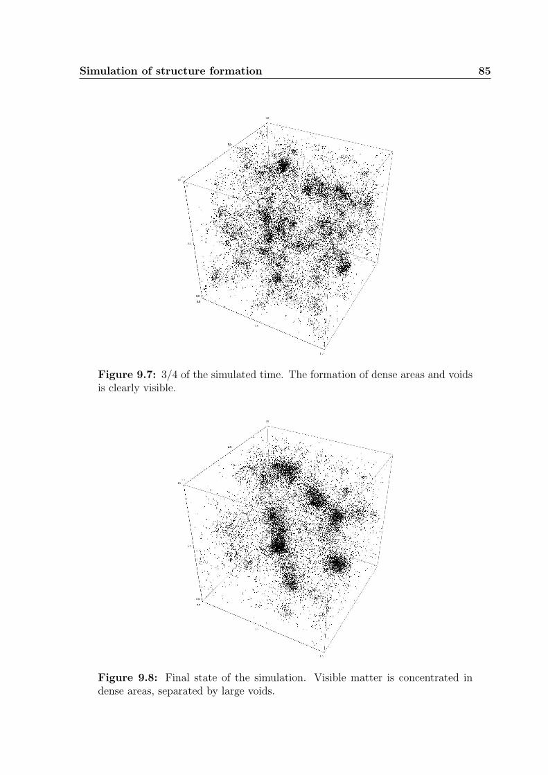
Simulation of structure formation 85
Figure 9.7: 3/4 of the simulated time. The formation of dense areas and voidsis clearly visible.
Figure 9.8: Final state of the simulation. Visible matter is concentrated indense areas, separated by large voids.

86

Chapter 10
Post-Newtonian analysis
We have discussed the cosmological dynamics of our repulsive multimetric gravity theory
in chapter 8 and derived a simple model for structure formation in chapter 9. We have
seen that the mutual repulsion between the different types of matter naturally leads to
an accelerating expansion of the universe and the formation of galactic voids which act
repulsively on visible matter.
In this chapter we will further test the predictions of our multimetric theory by high-
precision solar system experiments. For this purpose we will extend the parametrized
post-Newtonian (PPN) formalism to multimetric gravity and then apply it to our theory.
The contents of this chapter are based mainly on [56]. In section 10.1 we will briefly
review the formalism and explain its basic properties. We will construct an extension
of the PPN formalism to multimetric gravity theories in section 10.2 and find that this
leads to an extended set of PPN parameters. In section 10.3 we will show that a subset
of these extended PPN parameters can already be obtained from the linearized equations
of motion. We will apply this linearized formalism to our multimetric gravity theory
in section 10.4. We will find that these do not match the observed values, but we are
able to present an improved theory from which the correct values are obtained while the
cosmological results and the dynamics of structure formation are unchanged.
Note that within this chapter, we will deviate from our convention 8πGN = 1 for
the Newton constant, and use the normalization GN = 1 instead, as this is the standard
convention throughout the PPN literature.
87

88 Post-Newtonian analysis
10.1 Parametrized post-Newtonian formalism
Basic ingredient of the PPN formalism is an expansion of the geometric background in
orders of the velocity of the source matter. This is a weak field approximation around a
fixed background metric g0 in coordinates (x0, xα),
gab = g0ab + hab = g0
ab + h(1)ab + h
(2)ab + h
(3)ab + h
(4)ab . (10.1)
Higher than fourth velocity order O(4) is not considered. It turns out that not all
metric perturbations h(i)ab ∼ O(i) are relevant to describe the motion of test bod-
ies. Moreover certain components vanish due to Newtonian energy conservation or
time reversal symmetry. We now only list the relevant, non-vanishing components of
the metric perturbations. These are written in terms of the so-called PPN potentials
U, Vα,Wα,ΦW ,Φ1 . . .Φ4,A and constant PPN parameters β, γ, ξ, α1 . . . α3, ζ1 . . . ζ4 as
h(2)00 = 2U (10.2a)
h(2)αβ = 2γUδαβ (10.2b)
h(3)0α = −1
2(3 + 4γ + α1 − α2 + ζ1 − 2ξ)Vα −
1
2(1 + α2 − ζ1 + 2ξ)Wα , (10.2c)
h(4)00 = −2βU2 − 2ξΦW + (2 + 2γ + α3 + ζ1 − 2ξ)Φ1 + 2(1 + 3γ − 2β + ζ2 + ξ)Φ2
+ 2(1 + ζ3)Φ3 + 2(3γ + 3ζ4 − 2ξ)Φ4 − (ζ1 − 2ξ)A . (10.2d)
The spacetime dependent PPN potentials are Poisson-like integrals over the source mat-
ter energy density ρ, velocity vα, internal energy ρΠ and pressure p. Due to the virial
theorem, the energy density is associated a velocity order ρ ∼ O(2) while one assigns
ρΠ, p ∼ O(4). The only PPN potential at second velocity order is the standard Newto-
nian potential
U(x0, ~x) =
∫d3x′
ρ(x0, ~x′)
|~x− ~x′|. (10.3)
Similar integrals define the third order vector potentials
Vα(x0, ~x) =
∫d3x′
ρ(x0, ~x′)vα(x0, ~x′)
|~x− ~x′|, (10.4a)
Wα(x0, ~x) =
∫d3x′
ρ(x0, ~x′)vβ(x0, ~x′)(xα − x′α)(xβ − x′β)
|~x− ~x′|3, (10.4b)
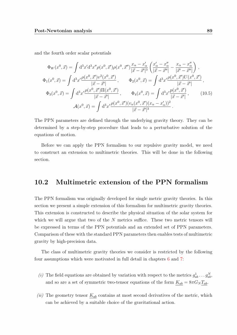
Post-Newtonian analysis 89
and the fourth order scalar potentials
ΦW (x0, ~x) =
∫d3x′d3x′′ρ(x0, ~x′)ρ(x0, ~x′′)
xα − x′α|~x− ~x′|3
(x′α − x′′α|~x− ~x′′|
− xα − x′′α|~x′ − ~x′′|
),
Φ1(x0, ~x) =
∫d3x′
ρ(x0, ~x′)v2(x0, ~x′)
|~x− ~x′|, Φ2(x0, ~x) =
∫d3x′
ρ(x0, ~x′)U(x0, ~x′)
|~x− ~x′|,
Φ3(x0, ~x) =
∫d3x′
ρ(x0, ~x′)Π(x0, ~x′)
|~x− ~x′|, Φ4(x0, ~x) =
∫d3x′
p(x0, ~x′)
|~x− ~x′|, (10.5)
A(x0, ~x) =
∫d3x′
ρ(x0, ~x′)(vα(x0, ~x′)(xα − x′α))2
|~x− ~x′|3.
The PPN parameters are defined through the underlying gravity theory. They can be
determined by a step-by-step procedure that leads to a perturbative solution of the
equations of motion.
Before we can apply the PPN formalism to our repulsive gravity model, we need
to construct an extension to multimetric theories. This will be done in the following
section.
10.2 Multimetric extension of the PPN formalism
The PPN formalism was originally developed for single metric gravity theories. In this
section we present a simple extension of this formalism for multimetric gravity theories.
This extension is constructed to describe the physical situation of the solar system for
which we will argue that two of the N metrics suffice. These two metric tensors will
be expressed in terms of the PPN potentials and an extended set of PPN parameters.
Comparison of these with the standard PPN parameters then enables tests of multimetric
gravity by high-precision data.
The class of multimetric gravity theories we consider is restricted by the following
four assumptions which were motivated in full detail in chapters 6 and 7:
(i) The field equations are obtained by variation with respect to the metrics g1ab . . . g
Nab,
and so are a set of symmetric two-tensor equations of the form Kab = 8πGNTab.
(ii) The geometry tensor Kab contains at most second derivatives of the metric, which
can be achieved by a suitable choice of the gravitational action.

90 Post-Newtonian analysis
(iii) The field equations are symmetric with respect to arbitrary permutations of the
sectors (gI ,ΨI), which can be understood as a generalized Copernican principle.
(iv) The vacuum solution is given by a set of flat metrics gIab = ηab. (Poincare symmetry
for all metrics simultaneously implies gIab = λIηab for constants λI that, invoking
the Copernican principle for the vacuum, should be equal and can be set to λI = 1.)
Cosmological constants are excluded because we are interested in multimetric gravity
theories in which the accelerating universe is modelled by a repulsive interaction between
different standard model copies, as we have seen in chapter 8.
Another consequence of the repulsion of matter from different sectors is their sepa-
ration as the universe evolves. Hence we may safely assume that the gravitational field
in regions like our solar system is dominated by a single type of matter; we formulate:
(v) Regions exist where the gravitational field is generated by matter sources from a
single sector.
Combining this assumption with the symmetry assumption (iii) guarantees the existence
of solutions in which the metric and the energy-momentum tensor corresponding to the
dominant matter source are distinct, while all other metric tensors are equal and their
energy-momentum tensors vanish. We assume that this simplest solution is actually
realized, since, as observers in a distinct region, we have no further detailed access to
the physics of the other sectors:
(vi) The metric tensors of all other sectors besides the one distinguished by the domi-
nant matter source are equal.
In the following we will indicate all quantities within the distinct sector I = 1 by a
superscript ‘+’, and all quantities within the other sectors by a superscript ‘−’. Hence
g+ab = g1
ab and T+ab = T 1
ab while g−ab = g2ab = . . . = gNab and T−ab = T 2
ab = . . . = TNab = 0. We
will now extend the standard single metric PPN formalism to this physical situation.
We start with a perturbative expansion of the metrics g±ab in analogy to the expansion
displayed in (10.1). The fixed background metric g0ab in this expansion is the flat vacuum
metric η by assumption (iv),
g±ab = ηab + h±ab = ηab + h(1)±ab + h
(2)±ab + h
(3)±ab + h
(4)±ab . (10.6)

Post-Newtonian analysis 91
We then write the metric perturbations h(i)±ab ∼ O(i) in terms of PPN potentials similar
to the standard PPN metric (10.2),
h(2)±00 = 2α±U , (10.7a)
h(2)±αβ = 2γ±Uδαβ + 2θ±Uαβ , (10.7b)
h(3)±0α = σ±+(Vα +Wα) + σ±−(Vα −Wα) , (10.7c)
h(4)±00 = −2β±U2 − 2ξ±ΦW + 2φ±1 Φ1 + 2φ±2 Φ2 + 2φ±3 Φ3 + 2φ±4 Φ4 + 2µ±A+ 2ν±B .
(10.7d)
Here we have introduced an additional scalar potential
B(x0, ~x) =
∫d3x′
ρ(x0, ~x′)∂0vα(x0, ~x′)(xα − x′α)
|~x− ~x′|, (10.8)
and a tensor potential
Uαβ(x0, ~x) =
∫d3x′
ρ(x0, ~x′)(xα − x′α)(xβ − x′β)
|~x− ~x′|3, (10.9)
both of velocity order O(4), and an extended set of PPN parameters α±, γ±, θ±, σ±±,
β±, ξ±, φ±1 . . . φ±4 , µ±, ν±.
The metric ansatz presented above fully reduces to the PPN formalism in single
metric theories. To see this, one simply drops all superscripts ‘±’. Moreover, it is then
conventional to choose a gauge so that the parameters θ and ν vanish, thus removing the
newly introduced potentials Uαβ and B. Also, one may choose α = 1 by absorbing its
value into the definition of the gravitational constant. In the extended PPN formalism
discussed here we have the same amount of freedom. However, gauge choices result from
diffeomorphism invariance and affect all metrics simultaneously, and also a rescaling of
the gravitational constant in one sector will affect the gravitational interaction between
all sectors. Hence only one of the two metrics g± can be simplified.
Since we wish to compare the multimetric PPN parameters to experimental data, we
turn our focus to observers that reside within the distinct sector, i.e., to observers for
whom the dominating matter source is visible. These observers as well as their visible
type of matter are affected by the metric g+ only. Thus g+ corresponds to the single
metric g in the standard PPN formalism. We will therefore choose a gauge in which h+
has the standard PPN form, i.e., θ+ = ν+ = 0, and fix the gravitational constant so
that α+ = 1. The remaining ten PPN parameters contained in h+ are then identified

92 Post-Newtonian analysis
with the PPN parameters known from the single metric case by direct comparison. The
conversion between the standard PPN parameters used in (10.2) and the notation we
use in the metric ansatz (10.7) is given by the relations
ζ1 = 2(ξ+ − µ+) , ζ2 = −1 + 2β+ − 3γ+ + φ+2 − ξ+ , ζ3 = −1 + φ+
3 ,
ζ4 = −1
3(3γ+ − φ+
4 − 2ξ+) , β = β+ , γ = γ+ , ξ = ξ+ , (10.10)
α1 = −4(1 + γ+ + σ++) , α2 = −1− 2(µ+ − σ+
− + σ++) , α3 = −2(1 + γ+ − µ+ − φ+
1 ) ,
or, equivalently,
β+ = β , γ+ = γ , ξ+ = ξ , φ+1 =
1
2(2 + 2γ + α3 + ζ1 − 2ξ) ,
φ+2 = 1 + 3γ − 2β + ζ2 + ξ , φ+
3 = 1 + ζ3 , φ+4 = 3γ + 3ζ4 − 2ξ , (10.11)
µ+ =1
2(2ξ − ζ1) , σ+
+ = −1
4(4 + 4γ + α1) , σ+
− = −1
4(2 + 4γ + α1 − 2α2 + 2ζ1 − 4ξ) .
With this identification we can convert the experimentally measured values of the stan-
dard PPN parameters to our notation and obtain
β+ = γ+ = φ+3 = 1 , φ+
1 = φ+2 = 2 , φ+
4 = 3 ,
ξ+ = µ+ = 0 , σ++ = −2 , σ+
− = −3
2. (10.12)
As we already argued in the introduction, these values are fixed by numerous experiments
within very narrow bounds. Gravity theories with significantly different PPN parameter
values are therefore experimentally excluded.
The values of the extended PPN parameters can now be computed in complete
analogy to the standard PPN formalism. We will examine this procedure in the following
section 10.3. Conveniently, it will turn out that some of the extended PPN parameters
can already be obtained from the linearized equations of motion.
10.3 Linearized PPN formalism
In the preceding section we have discussed an extension of the PPN framework to mul-
timetric gravity theories, which allows tests of these theories by means of available ex-
perimental data from solar system and astronomical experiments. We have shown that,

Post-Newtonian analysis 93
in addition to the parameters obtained from the standard PPN framework, we obtain
further parameters that characterize the influence of matter sources from one sector on
the metric tensors of the other sectors. In this section, we will show that a number of
the extended PPN parameters can be computed already from the linearized equations
of motion. This covers the PPN velocity orders up to O(3) while all terms of O(4) and
higher are neglected. We will give a step-by-step recipe for this calculation.
10.3.1 Geometry and matter content
The starting point for our computation is the most general linearized field equations
compatible with our assumptions stated at the beginning of section 10.2. Using the
convention GN = 1 for the normalization of Newton’s constant, these equations read
Kab = 8πT ab (10.13)
with the linearized geometry tensor
Kab = P · ∂p∂(ahb)p +Q ·�hab +R · ∂a∂bh+M · ∂p∂qhpqηab +N ·�hηab +O(h2)
(10.14)
and constant parameter matrices P,Q,R,M,N . Our assumptions pose two restrictions
on these matrices. First, the linearized equations of motion (10.13) are invariant under a
permutation of the sectors by assumption (iii). Hence the parameter matrices will have
the form
OIJ = O− + (O+ −O−)δIJ (10.15)
with diagonal entries O+ and off-diagonal entries O− for O = P,Q,R,M,N . This leaves
us with a set of ten parameters determined by the underlying (nonlinear) gravity theory.
Second, the equations of motion are tensor equations by assumption (i), and so the
linearized equations should be gauge-invariant. Using the formalism of gauge-invariant
perturbation theory detailed in section 6.2, one finds the invariance conditions
(P + 2Q) · 1 = (P + 2R) · 1 = (M +N) · 1 = 0 , (10.16)

94 Post-Newtonian analysis
where 1 = (1, . . . , 1)t and 0 = (0, . . . , 0)t denote N -component vectors. Using (10.15),
these conditions can be written in the form
P+ + (N − 1)P− + 2Q+ + 2(N − 1)Q− = 0 , (10.17a)
P+ + (N − 1)P− + 2R+ + 2(N − 1)R− = 0 , (10.17b)
M+ + (N − 1)M− +N+ + (N − 1)N− = 0 . (10.17c)
These equations fix three of the ten parameters in the parameter matrices so that the
most general linearized curvature tensor consistent with our assumptions is completely
determined by a set of seven parameters.
We will now turn our attention from the geometry side to the matter side of the
equations of motion. Recall that, according to assumption (v), we consider only so-
lutions of the field equations in which the gravitational field is generated by matter
sources within a single sector, i.e., by a single energy-momentum tensor T+, while all
other energy-momentum tensors T− must vanish. In order to solve the linearized field
equations (10.13), we need to expand T+ up to the required order of perturbation theory,
i.e., to velocity order O(3). We will use the ansatz
T+00 = ρ , T+
0α = −ρvα , T+αβ = 0 , (10.18)
corresponding to a perfect fluid of density ρ ∼ O(2) and velocity vα ∼ O(1).
10.3.2 Computation of the extended PPN parameters
We will now explicitly solve the equations of motion. Omitting all terms in the PPN
metric (10.7) corresponding to perturbations of velocity order O(4) we may use the
simplified ansatz
h±00 = −α±4χ , (10.19a)
h±0α = σ±+X+α + σ±−X
−α , (10.19b)
h±αβ = 2θ±∂α∂βχ− (γ± + θ±)4χδαβ . (10.19c)
These expressions are rewritten in terms of the so-called superpotential
χ(x0, ~x) = −∫
d3x′ρ(x0, ~x′)|~x− ~x′| (10.20)

Post-Newtonian analysis 95
using the relations
U = −1
24χ , Uαβ = ∂α∂βχ−
1
24χδαβ . (10.21)
We have furthermore introduced the notation X±α = Vα ±Wα for the vector potentials.
The advantage in using X±α instead of Vα and Wα results from the fact that X−α = ∂α∂0χ
is a pure divergence andX+α is a divergence-free vector, ∂αX+
α = 0. These relations follow
from the Newtonian continuity equation ∂0ρ + ∂α(ρvα) = 0 and the definitions (10.4),
and will be used repeatedly in the following computation.
We begin by performing a (1 + 3)-split of the equations of motion (10.13). Using the
energy-momentum tensor ansatz (10.18) we obtain the equations
K+00 = 8πρ , K−00 = 0 , (10.22a)
K+0α = −8πρvα , K−0α = 0 , (10.22b)
K+αβ = 0 , K−αβ = 0 . (10.22c)
In order to solve these equations, we expand the geometry tensor Kab given in (10.14)
using the PPN metric (10.19). In this calculation we once again drop all terms of velocity
order O(4), taking care of the fact that time derivatives count as ∂0 ∼ O(1). Up to the
required order O(3) the geometry tensor then takes the form
K±00 = c±144χ , (10.23a)
K±0α = c±24X+α + c±34X−α , (10.23b)
K±αβ = c±444χδαβ + c±54∂α∂βχ , (10.23c)
where the coefficients c±1 , . . . , c±5 are constants which depend linearly both on the PPN
parameters and the components of the parameter matrices (10.15). For a detailed ex-
pansion of these coefficients, see appendix B.
We will now determine the coefficients c±1 , . . . , c±5 such that the equations of motion
are satisfied for arbitrary matter distributions ρ and vα. First, we solve the scalar
equations (10.22a). Using the relation
44χ = −24U = 8πρ , (10.24)
one can see that these are solved if, and only if, the corresponding coefficients take the

96 Post-Newtonian analysis
values
c+1 = 1 , c−1 = 0 . (10.25)
We continue with the tensor equations (10.22c). Note that44χδαβ is a pure trace term,
while 4∂α∂βχ decomposes into a pure trace and a traceless part,
4∂α∂βχ = 44αβχ+1
344χδαβ , (10.26)
using the traceless second derivative 4αβ = ∂α∂β − δαβ4/3. In order for the tensor
equations to be satisfied, both the trace and the traceless part, and thus the coefficients
of both terms, must vanish,
c±4 = c±5 = 0 . (10.27)
Taking a closer look at the expansion of the coefficients displayed in appendix B, one
finds that the coefficients c±1 , c±4 , c
±5 only depend on the PPN parameters α±, γ±, θ±. We
therefore have obtained the six equations (10.25), (10.27) for six of the PPN parameters.
However, due to the gauge invariance conditions (10.17), these are linearly dependent.
In order to solve the equations, one needs to (partially) fix a gauge by fixing the value
of one of the parameters. The standard PPN gauge corresponds to the simple choice
θ+ = 0.
We now turn our attention to the vector equations (10.22b). The equation for K−0α
is easily solved using the fact that both the divergence-free and the total derivative part
of the curvature tensor, and thus both coefficients must vanish,
c−2 = c−3 = 0 . (10.28)
Finally, we consider the equation for K+0α which yields
c+24X+
α + c+34X−α = −8πρvα = 24Vα = 4(X+
α +X−α ) (10.29)
using the definition of Vα in the second equality. The equation above is now split into
pure divergence and divergence-free vector terms which decouple and have to be solved
independently. This results in
c+2 = c+
3 = 1 . (10.30)

Post-Newtonian analysis 97
Another close look at the newly obtained equations for c±3 and the expansions given
in appendix B reveals that all terms containing σ±− drop out due to the gauge invariance
conditions (10.17). The equations for c±3 then turn out to be linearly dependent on the
equations we have obtained from the scalar and tensor components of the equations of
motion, and thus they are solved identically. The remaining two equations for c±2 can
finally be used to solve for the PPN parameters σ±+.
To summarize, the linearized field equations in our multimetric PPN framework al-
ready are strong enough to determine the eight extended PPN parameters α±, γ±, θ±, σ±+.
These parameters are the solutions of equations (10.25), (10.27), (10.28) and (10.30).
Given any particular multimetric theory consistent with our assumptions, one may use
this result as a quick test of solar system consistency, simply by comparing the predicted
PPN parameters with the experimentally favoured results (10.2). Before analyzing the
particular theory proposed in chapter 7 in the following section we remark that a calcu-
lation of the remaining PPN parameters in the extended multimetric formalism requires
higher order perturbation theory that also covers velocity orders O(4). In practice this
is a very lengthy calculation that we do not wish to enter in this thesis, but it poses no
difficulty in principle.
10.4 Application to the repulsive gravity model
We will now determine the PPN parameters α±, γ±, θ±, σ±+ of the repulsive gravity model
proposed in chapter 7 by applying the multimetric PPN formalism developed in the
previous sections. For this purpose we first derive the linearized field equations and
determine the parameter matrices P ,Q,R,M,N that appear in the linearized curvature
tensor (10.14). Second, we follow the steps detailed in section 10.3.2 in order to compute
the PPN parameters of our theory explicitly. It will turn out that these do not agree
with the values obtained from experiments. But this problem can be solved, as we will
finally show, by simple correction terms that improve the action of our theory. The
calculated PPN parameters of the improved theory are now consistent with experiment,
and the theory features the same accelerating late-time cosmology.

98 Post-Newtonian analysis
10.4.1 Linearized field equations
The starting point for our computation is the field equations (7.16). Using the convention
GN = 1, these read
KIab = 8πT Iab (10.31)
with the geometry tensor defined in (7.17). We now derive the linearized field equations
using the perturbative ansatz gIab = ηab+hIab. Note that the connection differences SIJijk
and the Ricci tensor RIij are of first order in the metric perturbations hI , so any terms
containing products of two connection differences drop out; covariant derivatives acting
on connection differences are replaced by ordinary partial derivatives; the metric tensors
gI are replaced by the flat metric η whenever they appear in a product with a connection
difference or Ricci tensor. These handy rules significantly simplify the computation and
one finally obtains the linearized geometry tensor
KIab =
N∑J=1
[ (2x− (Nx− y)δIJ
)∂p∂(ah
Jb)p +
(−x+
1
2(Nx− y)δIJ
)�hJab
+
(Nx
2δIJ − x− y
2N
)∂a∂bh
J +
(Nx
2δIJ − x− y
2N
)∂p∂qh
Jpqηab
+
(x+
y
N− Nx+ y
2δIJ)�hJηab
]+O(h2) .
(10.32)
Comparing this equation with the most general form of the linearized geometry ten-
sor (10.14) and writing the parameter matrices in the form (10.15), we read off the
parameter values
P+ = (2−N)x+ y , P− = 2x , (10.33a)
Q+ =N − 2
2x− y
2, Q− = −x , (10.33b)
R+ =N − 2
2x− y
2N, R− = −x− y
2N, (10.33c)
M+ =N − 2
2x− y
2N, M− = −x− y
2N, (10.33d)
N+ =2−N
2x+
2−N2N
y , N− = x+y
N. (10.33e)
These values of course satisfy the gauge-invariance conditions (10.17), since they result
from a diffeomorphism invariant gravitational action. We are now in the position to

Post-Newtonian analysis 99
follow the steps detailed in section 10.3.2 to compute the PPN parameters of our theory.
10.4.2 PPN parameters
With the parameter values of the linearized theory obtained in (10.33) we now compute
the PPN parameters α±, γ±, θ±, σ±+ of our repulsive gravity model defined by (7.3) and
(7.1). The procedure for this is based on solving the equations of motion, for which we
developed the technology in section 10.3.2. Choosing the standard PPN gauge such that
θ+ = 0 yields the PPN parameters
α+ =1
3N
(3
Nx+ y− 4N − 4
Nx− y
), α− =
1
3N
7Nx+ y
N2x2 − y2,
γ+ =1
3N
(3
Nx+ y− 2N − 2
Nx− y
), γ− =
1
3N
(3
Nx+ y− N − 2
Nx− y+N
y
),
θ+ = 0 , θ− =1
3Nx− 3y− 1
3y, (10.34)
σ++ =
(2N − 4)x+ 2y
N2x2 − y2, σ−+ = − 4x
N2x2 − y2.
We now focus on the Newtonian limit of our theory. Recall that we demand a
Newtonian limit where the gravitational interaction within each sector is attractive,
while it is repulsive of equal strength between matter belonging to different sectors. This
limit corresponds to the PPN parameters α+ = 1 and α− = −1. These are achieved for
parameter values
x =2N − 1
6N(2−N), y =
−2N + 7
6(2−N). (10.35)
Note that this recovers the same values (7.20) that can also be obtained from a purely
Newtonian calculation. Substituting these values into (10.34) simplifies the results for
the PPN parameters to
α+ = 1 , α− = −1 ,
γ+ =1
N, γ− =
3
2N − 7+
1
N+
1
2,
θ+ = 0 , θ− =1
7− 2N− 3
2, (10.36)
σ++ = −1− 1
N, σ−+ = 2− 1
N.

100 Post-Newtonian analysis
Comparison with the observed values γ+ = 1 and σ++ = −2 displayed in (10.2) immedi-
ately shows that these are satisfied only in the case N = 1, i.e., when there is only one
metric and a corresponding copy of the standard model, in which case our theory reduces
to Einstein gravity. This is a dissatisfactory result since our aim was the construction
of experimentally feasible gravity theories for N > 1.
This result shows that our model requires modification in order to match exper-
imental bounds from solar system experiments. In the following we will make such
improvements that adapt the theory to the observed values of the PPN parameters.
10.4.3 Improved PPN consistent theory
Since the PPN parameters calculated for our theory do not match the observed values, it
is natural to ask whether the theory can be modified so to reproduce the correct values.
We will now show that this is indeed possible.
We will modify the action and then proceed in complete analogy to the previous
sections. First, we will compute the field equations from a variation of the modified
action. Second, we will expand the metric around a flat solution and derive the linearized
field equations. Third, we will read off the values of the parameter matrices and employ
the linearized multimetric PPN formalism constructed in section 10.3.2. We will only
give a brief sketch of this calculation here.
We start from the gravitational action (7.3) and add the following term which is
consistent with our assumptions (i)–(iv) of section 10.2 that restrict the multimetric
theories we consider in this part of the thesis:
SG =1
16π
N∑I=1
∫d4x√g0 g
I ij(zSIkS
I kij + uSI iS
Ij
). (10.37)
This term contains two new constant parameters z, u that will be determined by PPN
consistency below. Note that the above modification is not the only possibility to achieve
experimental consistency of our model. Even within the class of quadratic connection
difference terms, one could discuss other examples of modification, with even more addi-
tional parameters, that also yield correct PPN values. The linearized multimetric PPN
formalism developed in section 10.3 does not well distinguish theories of this type.
We continue by computing the equations of motion by variation. These take the

Post-Newtonian analysis 101
form displayed in equations (10.31), but the curvature tensor KIab in (7.17) attains a
correction term KIab that is rather involved. We then compute the linearized curvature
tensor. In addition to the result obtained in (10.32) this gives
KIab =
z
2ηabη
ij∂kSI kij +
2u− z2
ηabηij∂iS
Ij + z∂(aS
Ib) +O(h2)
=∑J
(− 1
N+ δIJ
)(z
2∂a∂bh
J +z
2∂p∂qh
J pqηab +z − u
2�hJηab
)+O(h2) .
(10.38)
Next, we read off the modified parameter matrices P ,Q,R,M,N . Using the nota-
tion introduced in section 10.3.1, we obtain the following modified results as compared
to (10.33):
P+ = (2−N)x+ y , P− = 2x , (10.39a)
Q+ =N − 2
2x− y
2, Q− = −x , (10.39b)
R+ =N − 2
2x− y
2N+N − 1
2Nz , R− = −x− y
2N− z
2N, (10.39c)
M+ =N − 2
2x− y
2N+N − 1
2Nz , M− = −x− y
2N− z
2N, (10.39d)
N+ =2−N
2x+
2−N2N
y +N − 1
2N(z − u) , N− = x+
y
N− z − u
2N. (10.39e)
Finally, we follow the steps detailed in section 10.3.2 to compute the PPN parameters
α±, γ±, θ±, σ±+. In comparison to (10.34) these take the modified values
α+ =1
3N
(3
Nx+ y− 4N − 4
Nx− y− 2(N − 1)(u− 3z)
Ξ
),
α− =1
3N
(7Nx+ y
N2x2 − y2+
2(u− 3z)
Ξ
),
γ+ =1
3N
(3
Nx+ y− 2N − 2
Nx− y+
2(N − 1)(u− 3z)
Ξ
),
γ− =1
3N
(3
Nx+ y− N − 2
Nx− y+N
y+
(4N − 2)u+ (6− 9N)z + 3Ny
Ξ
), (10.40)
θ+ = 0 , θ− =1
3Nx− 3y− 1
3y− 4u+ 3(y − 3z)
3Ξ,
σ++ =
(2N − 4)x+ 2y
N2x2 − y2, σ−+ = − 4x
N2x2 − y2.
for Ξ = 3(y2 + z2)− 2Nx(u− 3z) + 2uy. One can now choose the parameters x, y, z, u
so that not only the Newtonian limit agrees with our repulsive gravity requirement

102 Post-Newtonian analysis
α+ = −α− = 1, but also the observed PPN parameter values γ+ = 1 and σ++ = −2 are
obtained. These results are achieved for parameter values
x =1
8− 4N, y =
4−N8− 4N
, z = − 4−N8− 4N
, u = −12− 3N
8− 4N. (10.41)
The remaining PPN parameters then are determined to be γ− = −1, θ− = 0 and σ−+ = 2.
Now that the PPN parameters of the improved model are consistent as far as we can
determine from the linearized multimetric PPN formalism, one may ask whether the
remarkable cosmological features of the original theory presented in chapter 8, such as
the accelerating late time expansion and the big bounce, and the dynamics of structure
formation presented in chapter 9 are still present in the improved version.
It can easily be seen that this is the case by noting that the modification (10.37)
of the action is quadratic in the connection difference tensors SIJ . Consequently the
additional terms in the equations of motion caused by this modification contain at least
one connection difference tensor. The remains of these are also seen in the linearized
term (10.38). For our simple cosmological model we assumed that a cosmological version
of the Copernican principle holds in the sense that equal amounts of each type of matter
are distributed homogeneously in our universe, and thus we could argue that all metric
tensors of the cosmological solution should be equal at very early and very late times. It
then follows that the connection differences vanish and the earlier obtained cosmological
equations of motion are unchanged under the modifications we presented in this section.
This also holds for the dynamics of structure formation, which are solely based on the
cosmological equations of motion and the Newtonian limit of our theory.

Chapter 11
Discussion
In this part of the thesis we followed the idea that a repulsive version of gravity might be
responsible for the observed accelerating expansion of the universe. We first discussed the
concept of negative mass in Newtonian gravity and then showed that the incorporation
of this concept into Einstein gravity naturally leads to a theory with N > 1 copies of
standard model matter, each of which is governed by its own metric tensor. We further
restricted the class of multimetric theories under consideration by the requirement that
each of the N matter sectors appears dark to observers residing in a different sector,
and demanded a Newtonian limit in which the gravitational interaction between the
different sectors is repulsive of equal strength compared to the attractive gravitational
interaction within each sector.
Starting from this idea, we first considered the simplest possible case N = 2 of
bimetric gravity. Using the formalism of gauge-invariant perturbation theory, we could
prove a theorem ruling out the possibility of bimetric theories compatible with our
assumptions. This led us to the conclusion that N ≥ 3 is a necessary condition for
repulsive gravity. We then showed that it is also sufficient by explicitly constructing a
theory of this type. We further examined various aspects of this particular theory.
Since it was our primary motivation to explain the accelerating expansion of the
universe using repulsive gravity, we derived a simple model for the cosmology of a ho-
mogeneous and isotropic universe and studied its dynamics by computing and solving
the cosmological equations of motion. It turned out that this model indeed features an
accelerating expansion and that the acceleration naturally becomes small for late times.
Besides these properties, we found that the universe must be open, and that a big bang
103

104 Discussion
is avoided in favor of a big bounce.
We then discussed local perturbations around this cosmological solution using meth-
ods from computational physics. We developed a simple model for the dynamics of
inhomogeneous matter distributions within our cosmological background and showed
that it leads to the formation of filament-like structures and voids for each matter type,
similar to the structures found in our universe by deep-sky surveys. It further turned
out that at the final stages of our simulated structure formation, the voids of one, say,
the visible, type of matter are not empty, but filled with matter of the other types and
thus act repulsively on visible matter. This provides a potential explanation for the local
velocity anomaly.
In order to further test our repulsive gravity model, we constructed an extension of
the parametrized post-Newtonian (PPN) formalism to multimetric gravity theories. We
found that this extended formalism features a larger set of PPN parameters, part of
which can already be obtained from the linearized field equations. We then applied this
linearized formalism to our particular gravity theory and computed its PPN parameters.
It turned out that these do not match the observed values, but we could improve the
theory so that the correct PPN parameter values are obtained. We finally showed that
the improved PPN consistent theory still features the same dynamics for cosmology and
structure formation.

Part II
Quantum manifolds
105


Chapter 12
Introduction
This part of the thesis addresses the quantization problem of gravity discussed in sec-
tion 3.2. Our aim is the construction of a mathematical framework that unifies both
the standard function space construction of quantum mechanics and the differentiable
manifold structure of classical spacetime, and might therefore be a suitable ingredient
for a quantum theory of gravity. Before we discuss the details of this construction, we
give a short motivation and explain the basic ideas that lead to this approach.
Current research on quantum gravity can be classified into essentially two different
approaches; the first is quantization, the second could be termed quantum construction.
Perhaps not surprisingly, the two main contenders at present for a full theory of quantum
gravity, namely string theory and loop quantum gravity, both are based on the quanti-
zation of a well-understood classical theory. As is well-known, gravity comes into string
theory through the requirement that the conformal invariance of the classical string also
hold in the quantum theory, which yields various supergravity theories as low energy
effective descriptions of quantum strings [91]. From the geometric point of view these
metric theories easily recover the classical manifold. However, a number of questions
about the geometric interpretation of the background fields besides the metric, such as
the dilaton and Neveu-Schwarz two form, remain open. A lot of work recently goes to-
wards understanding the role of these generalized backgrounds [45, 60, 96, 134, 106, 48].
Loop quantum gravity on the other hand is based on canonical quantization of Einstein’s
general relativity in Ashtekar variables [114, 102]. A number of promising results like the
quantization of the area and volume operators has been obtained in this framework, and
applied, for example, to the discussion of the big bang in the very early universe [6, 17].
However, the geometric interpretation of loop quantum gravity is still largely unresolved;
107

108 Introduction
although the theory originates from a metric classical background, it so far lacks the re-
emergence of the manifold geometry from the spin network states in a suitable classical
limit [83].
The main idea behind quantum construction is that the classical manifold picture
of spacetime should be changed, even break down, at small length scales comparable
to the Planck length, or at very high energy scales. Thus one starts out with quantum
modifications of the basic background structures, in some sense reversing the procedure
of quantization. A wide-ranging number of ideas fall into this category. On the phe-
nomenological level many approaches consider the emergence of modified energy momen-
tum dispersion relations [3, 43]. A geometrical basis for such an assumption, however, is
rarely given [103]. On the rigorous mathematical side there are various ideas for the dis-
cretization of spacetime, such as the description of spacetime as a causal set [113, 18] or
via dynamical triangulations [2], or for the short-distance modification of spacetime for
instance by non-commutative geometry [21, 26]. Some of the mathematically rigorous
approaches are not easily interpreted in terms of a smooth classical limit manifold.
Our work in this part of the thesis falls within the second category of quantum
construction; we construct and explore a modified structure of spacetime, rather than
quantizing a given classical theory. We are conservative in the sense that we use as main
ingredients ideas already known from other work on the geometry of quantum theory;
one such idea is that of infinite-dimensional manifolds [66, 67, 23, 24, 63]. However, we
employ this idea in a very different way. More precisely, we propose a mathematical
model of quantum spacetime based on an infinite-dimensional manifold locally home-
omorphic to an appropriate space of Schwartz functions. The idea behind this is as
follows. Consider the space Rn as the simplest arena for classical mechanics, i.e., as the
space of positions providing labels for classical physical events. This background appears
as the limit of two more general constructions, as shown in the diagram in figure 12.1.
The first is the manifold geometry at the heart of general relativity, where spacetime is
locally homeomorphic to Rn; in this setting the idea of labels for events is taken seriously
in the sense that different labellings can be chosen provided they are diffeomorphic. The
second construction reducing to Rn is that of quantum mechanics. Here observables be-
come operators on a Hilbert space, or more accurately, on the Schwartz space S(Rn) of
fast-decreasing functions over Rn, which is reobtained as the set of all possible position
expectation values.
The mathematical construction that we present below unifies both the manifold and
function space ideas, which might be seen as the fundamental structures behind general

Introduction 109
M aa
local homeomorphism !!!a!a!a!a
S
position expectation~~}}}}
}}}}
Rn
Figure 12.1: Manifold geometry M and quantum function spaces S limiting toRn.
relativity and quantum theory, respectively. We are able to complete the diagram above
by introducing the geometry of a quantum manifold MQ that is, on the one hand,
locally homeomorphic to the Schwartz space S(Rn), and, on the other hand, allows the
computation of position expectation values that recover the classical manifold. This idea
is nicely expressed in the completed diagram of figure 12.2. We wish to emphasize that
it will be a feature of the mathematical structure of the quantum manifold explicitly to
avoid the problems of other quantum constructions with the classical limit.
MQ ``local homeomorphism
` ` ` `position expectation
}}{{{{
{{{{
M bb
local homeomorphism """b"b"b"b"b
S
position expectation}}{{{{
{{{{
Rn
Figure 12.2: Quantum manifold MQ unifying manifold geometry M and quan-tum function spaces S.
To put our proposal into a bigger perspective, we might speculate that physics should
be formulated as field theories over the quantum manifold; seen from the classical per-
spective these theories should thus at the same time be geometrically well-defined and
show quantum behaviour. In other words, if this can be made precise, classical fields on
the quantum geometry would become quantum fields on the classical geometry. Then
this would also lead to an exciting new formulation of quantum gravity, simply as a
classical geometric gravity theory on the infinite-dimensional quantum manifold, which
becomes quantum from the point of view of the classical observer.
In this part of the thesis, which is mainly based on [53], we take the first impor-

110 Introduction
tant step in this program. We transform the idea of the quantum manifold into a
concrete, and mathematically precise, geometric concept, and explore some of its prop-
erties. In sections 13.1 and 13.2, we briefly review the required notions of elementary
topology and topological vector spaces. Section 13.3 discusses the Schwartz space on
which we will model our quantum geometry. The infinite-dimensional quantum mani-
fold is precisely defined in section 14.1. In section 14.2 we prove the central result that
a finite-dimensional differentiable manifold emerges as a classical limit by topological
identification of functions with coinciding position expectation values. Moreover, we are
able to show in section 15.1 that any quantum manifold carries the structure of a fiber
bundle over its associated classical limit. Section 15.2 demonstrates that any classical
manifold can be trivially quantized, which ensures the existence of quantum manifolds.
We speculate on potential physical interpretations in chapter 16. We end with a discus-
sion in chapter 17. The proofs to some of the results stated in the main text are deferred
to appendix C.
Chapter 13
Mathematical ingredients
Before we proceed with our quantum manifold construction, we briefly review the nec-
essary mathematical ingredients in this chapter. We begin with the most elementary
notions of topology in section 13.1 and topological vector spaces in section 13.2. We
then turn our focus to a particular topological vector space, known as Schwartz space,
in section 13.3.
13.1 Elementary topology
Recall that a topology is one of the most elementary structures on a set of points, where
it provides neighborhood relations by specifying the notion of open sets. To be precise,
a topology T on a set X is a system of subsets of X, called the open sets, which satisfies
the following three properties: (i) the empty set ∅ and the whole set X itself are open,
i.e., they are elements of T , (ii) any finite intersection of open sets is open, and, (iii) any,
also infinite, union of open sets is open. The pair (X, T ) is called a topological space.
A given set X may be equipped with different topologies, say with T1 and T2. Con-
sider the special case T1 ⊂ T2, i.e., that all open sets of X contained in the topology T1
are also contained in T2; then we call T1 coarser (weaker) than T2, and T2 finer (stronger)
than T1.
A map f : X → Y between two topological spaces (X, T ) and (Y, T ′) is called
continuous if and only if the pre-image of any open set is open, i.e., if for all V ∈ T ′
also f−1(V ) ∈ T .
111

112 Mathematical ingredients
Two points x, y ∈ X of a topological space (X, T ) are called topologically indistin-
guishable, if the open sets containing x are precisely the open sets containing y. In other
words, it is not possible to find an open set around one of the points that does not
also contain the other. It is not difficult to see that topological indistinguishability on
a topological space (X, T ) is an equivalence relation ∼. It proves useful to consider the
equivalence classes [x] = {y ∈ X|y ∼ x} of this relation and their collection.
The Kolmogorov quotient of (X, T ) is a topological space (Y, T ′), where Y is the set
of all equivalence classes of topologically indistinguishable elements of X and a subset
of Y is open, if and only if its pre-image under the natural surjection X → Y, x 7→ [x]
is open.
Let X be a set and hi : X → Yi, i ∈ I a family of functions, mapping into topological
spaces (Yi, Ti). The initial topology on X with respect to (hi, i ∈ I) is the topology
generated by the pre-images h−1i (Vi), where Vi ⊂ Yi is open. It is the coarsest topology
on X such that all functions hi are continuous.
Let ((Xi, Ti), i ∈ I) be a family of topological spaces, X their product space and
πi : X → Xi the projection onto the i-th factor. The product topology on X is the initial
topology with respect to the family (πi, i ∈ I) of projections.
Let (E, TE), (B, TB), (F, TF ) be topological spaces and π : E → B a continuous
surjection. The space E is called a fiber bundle over B with typical fiber F and projection
π, if for each x ∈ B there exists an open set U ∈ TB with x ∈ U and a homeomorphism
h : π−1(U)→ U × F , such that the following diagram commutes:
π−1(U)h //
π
��
U × F
p1
yysssssssssss
U
(13.1)
Here, p1 denotes the projection onto the first factor U .
13.2 Topological vector spaces
Topological vector spaces are central to the definition of the differentiability of functions.
They combine the notions of vector spaces and topological spaces in a compatible way.
To be precise, a topological vector space (E, TE) over a field K is a K-vector space E

Mathematical ingredients 113
together with a topology TE on E, so that the operations of addition + : E × E → E
and multiplication by a scalar · : K×E → E are continuous. This reflects the intuitive
picture that both the translation of open sets by constant vectors and their rescaling by
nonzero factors again yield open sets.
Given two topological vector spaces (E, TE) and (F, TF ) we are now able to define
the notion of differentiability for functions f : E → F , see [68]. We call f differentiable
in v0 ∈ E, if it can be locally approximated by a linear function, i.e., if there exists a
linear function λ : E → F and a neighborhood V ⊂ E of v0, such that
f(v0 + v) = f(v0) + λ(v) + δ(v) (13.2)
for all v0 + v ∈ V and δ is sufficiently small. λ is called the derivative of f in v0, and
denoted by the differential Df(v0).
Of course, we need to clarify what it means for δ to be sufficiently small. This is the
case when δ is a so-called tangent to zero. For V ⊂ E an open neighborhood of 0 and
δ : V → F , the map δ is said to be tangent to zero, if for all open neighborhoods W ⊂ F
of 0 there exists an open set V ⊂ V , a positive number ε and a function o : [−ε, ε]→ R,
such that
limt→0
o(t)
t= 0 (13.3)
and δ(tV ) ⊂ o(t)W for all t ∈ [−ε, ε]. Intuitively, this means that the pre-images of open
neighborhoods W ⊂ F of 0 under δ shrink faster than linearly with the scaling factor of
W .
13.3 Model spaces
We aim at a model for quantum spacetime that unifies key ingredients both from general
relativity and quantum theory. As motivated in the introduction, the first ingredient
we choose is the geometric structure of a manifold, the second is the notion that func-
tion spaces should play a major role. Thus we will construct a very specific infinite-
dimensional manifold that is locally homeomorphic to a function space. Since we are
interested in a quantum spacetime model with a classical limit we will also tie in the
idea of position expectation values. In extension of standard quantum mechanics, we will
find it appropriate for our needs to model the infinite-dimensional quantum manifold on

114 Mathematical ingredients
the Schwartz space S(Rn) of fast-decreasing functions over Rn. In this section we will
discuss this model space in more detail, as a necessary and important preparation for
the definition of the quantum manifold in the next section.
First consider the Hilbert space L2(Rn) of square-integrable complex functions over
Rn with the scalar product
〈f, g〉 =
∫Rn
dx f(x)∗g(x) (13.4)
between two functions f and g. We canonically define the position operators Qi and the
momentum operators Pi for i = 1 . . . n; they act on functions f as (Qif)(x) = xif(x)
and (Pif)(x) = −i∂if(x). These operators are not defined on the whole of L2(Rn) since
their application may destroy square-integrability. They are, however, defined on the
Schwartz space S(Rn), which is a dense subset of L2(Rn) and closed under the operation
of Q and P :
S(Rn) ={f ∈ C∞(Rn) | ∀α,β ∈ Nn : sup
x∈Rn
|xαDβf(x)| <∞}. (13.5)
For later convenience we define S 6=0(Rn) as the Schwartz space with the zero function
removed,
S 6=0(Rn) = S(Rn) \ {0} . (13.6)
The Schwartz space, and by restriction also S 6=0(Rn), are topological spaces. The family
‖f‖α,β = supx∈Rn
|xαDβf(x)| (13.7)
for all multiindices α,β is a family of seminorms which generates a topology on S(Rn).
This topology is called the natural topology. Constructively, it is generated by the open
balls V rα,β(f0) of radius r > 0 around f0 ∈ S(Rn),
V rα,β(f0) = {f ∈ S(Rn) | ‖f0 − f‖α,β < r} . (13.8)
We will now take a closer look on the respective topological duals (L2(Rn))∗ and
(S(Rn))∗ of the Hilbert space and the Schwartz space, and their relations. By definition
the topological dual is the space of linear functionals. Consider first the Hilbert space
L2(Rn). By the Riesz representation theorem the Hilbert space and its topological

Mathematical ingredients 115
dual are isomorphic via the map L2(Rn) → (L2(Rn))∗, f 7→ f † where f † is defined
by the scalar product as f †(g) = 〈f, g〉. Now note that the Schwartz space is not a
Hilbert space, but that we have a natural injection S(Rn) ↪→ L2(Rn). The dual of the
Schwartz space is known as the space of tempered distributions. There exists a natural
injection (L2(Rn))∗ ↪→ (S(Rn))∗; indeed, recalling that the elements of (L2(Rn))∗ are
linear functionals on L2(Rn), the injection is simply their restriction to S(Rn). The
composition of the two injections and the isomorphism of L2(Rn) onto its dual induces
an anti-linear injection S(Rn) ↪→ (S(Rn))∗. Working with the Schwartz space and its
topological dual hence is nothing else than working with the Gelfand triple [16], or rigged
Hilbert space,
S(Rn) ⊂ L2(Rn) ∼= (L2(Rn))∗ ⊂ (S(Rn))∗ . (13.9)
To link our construction below of the infinite-dimensional quantum manifold with
the classical finite-dimensional picture of spacetime we will exploit the idea of position
expectation values. As usual, the expectation value of a linear operator O : S → S is
the map O : S 6=0 → R defined by
O(f) =〈f,Of〉〈f, f〉
. (13.10)
Hence, for any f ∈ S 6=0 the position expectation value is the vector (Q(f))i = Qi(f).
The position expectation value allows us to define a very special topology on S 6=0(Rn),
which we will call the expectation value topology. We will see below that this topology
is essential in the definition of the quantum manifold and the recovery of classical space-
time. We take the expectation value topology to be the initial topology ι(S 6=0(Rn), Q)
with respect to Q. The definition, see section 13.1, implies that the open sets of the
expectation value topology are precisely of the form
Q−1(W ) ={f ∈ S 6=0 | Q(f) ∈ W
}, (13.11)
where W ⊂ Rn is open in the standard topology on Rn. Thus this is the coarsest
topology in which the function Q is continuous.
Note that every set V ⊂ S(Rn) that is open in the initial topology is also open
in the natural topology defined above. This is equivalent to the statement that Q is
also continuous with respect to the natural topology on S(Rn). We will prove this

116 Mathematical ingredients
statement in appendix C. There we will also prove that Q is not merely continuous but
also differentiable with respect to the natural topology on S(Rn). Both these properties
of Q will be needed as key ingredients when we construct the classical limit of a quantum
manifold and show that it is in fact a differentiable manifold.
For practical computations, it is often convenient to use a different family of semi-
norms on the Schwartz space S(Rn). These seminorms are given by
‖f‖p =⟨f, (Q2 + P 2 + 1)pf
⟩(13.12)
for all f ∈ S(Rn) and p ∈ N. They generate the so-called nuclear topology on S(Rn) via
the open balls V rp (f0) of radius r > 0 around f0 ∈ S(Rn),
V rp (f0) = {f ∈ S(Rn)|‖f0 − f‖p < r} . (13.13)
It can be shown that the two families of seminorms (‖f‖p, p ∈ N) and (‖f‖α,β, α,β ∈Nn) generate the same topology [99], i.e., sets are open in one topology if and only if
they are in the other. Therefore, we may use the words nuclear topology and natural
topology synonymously, and any statement valid for one of them will also be valid for
the other.

Chapter 14
Construction of a quantum manifold
The Schwartz space of functions together with certain useful topologies has been dis-
cussed in some detail in the previous section. This space will now become the model
space in our quantum manifold construction, and we are now in the position to present
the central definitions of this part of the thesis. Following the construction of classical
manifolds in [68], we will proceed to define the quantum manifold in section 14.1 by
first, equipping a basic set with an atlas, and second, by considering equivalence classes
of compatible atlases. In section 14.2 we will then show that every quantum manifold
has a classical limit manifold which can be obtained by taking its Kolmogorov quotient.
14.1 Basic construction
We begin with the definition of a quantum atlas of dimension n ∈ N on a set MQ. The
quantum atlas is a collection of pairs A = {(Ui, φi), i ∈ I} for some index set I, called
charts, which satisfy the following four conditions:
(i) Each Ui is a subset of MQ and the Ui cover MQ.
(ii) Each φi is a bijection of Ui onto a set φi(Ui) ⊂ S 6=0(Rn).
(iii) For each i, j, the set φi(Ui∩Uj) is open in the expectation value topology ι(S 6=0(Rn), Q).
(iv) For each i, j, the transition map
φji = φj ◦ φ−1i (14.1)
117

118 Construction of a quantum manifold
on the overlap of any two charts, φji : φi(Ui ∩ Uj) → φj(Ui ∩ Uj) is continuous in
the expectation value topology and differentiable in the natural topology.
From this definition, it is clear that the final quantum manifold will be a differentiable
infinite-dimensional manifold locally homeomorphic to S 6=0(Rn). In contrast to the usual
definition of an atlas, two different topologies are introduced. We will see in the following
section that this is central for the existence of a classical limit. Before we can state the
definition of the quantum manifold, we need to consider equivalence classes of compatible
atlases.
Two quantum atlases A,A′ of common dimension n on a set MQ are said to be
compatible, if also their union A ∪ A′ is a quantum atlas of dimension n on MQ. Note
that compatibility of quantum atlases so defined is an equivalence relation. Reflexivity
and symmetry are immediate, so we only need to check that compatibility of atlases is
transitive: given three atlases A,A′,A′′ with A ∪ A′ and A′ ∪ A′′ also being atlases,
A ∪ A′′ should also be an atlas. We now check the conditions from the definition in
turn. Clearly, A ∪ A′′ is a collection of pairs (Ui, φi), where the Ui cover MQ and the
φi are bijections of Ui onto subsets of S 6=0(Rn), which gives conditions (i) and (ii). We
still have to check the remaining two, namely, that for all i, j, the sets φi(Ui ∩ Uj) are
open in the expectation value topology of S 6=0(Rn) and the maps φji = φj ◦ φ−1i are
continuous in the expectation value topology and differentiable in the natural topology.
These properties are obvious in the case that both (Ui, φi) and (Uj, φj) belong to either
one of the atlases A or A′′, but we have to make sure that this is also true for (Ui, φi) ∈ Aand (Uj, φj) ∈ A′′. Let this be the case, and let A′ = {(Uk, φk), k ∈ K}. Using the fact
that the Uk cover MQ, we may write
φi(Ui ∩ Uj) =⋃k∈K
φi(Ui ∩ Uj ∩ Uk) =⋃k∈K
(φik ◦ φk)((Ui ∩ Uk) ∩ (Uj ∩ Uk))
=⋃k∈K
φ−1ki (φk(Ui ∩ Uk) ∩ φk(Uj ∩ Uk))
(14.2)
Both φk(Ui∩Uk) and φk(Uj∩Uk) are open, sinceA∪A′ andA′∪A′′ are atlases; hence their
intersection is open. Since φki is continuous, the pre-image of this intersection is open.
Finally, since any union of open sets is open, φi(Ui ∩ Uj) is open, which shows property
(iii). To see that φji = φj ◦ φ−1i is continuous and differentiable in ψ ∈ φi(Ui ∩ Uj), we
choose k ∈ K such that φ−1i (ψ) ∈ Uk and consider the map
φji|φi(Ui∩Uj∩Uk) = φjk|φk(Ui∩Uj∩Uk) ◦ φki|φi(Ui∩Uj∩Uk) . (14.3)

Construction of a quantum manifold 119
Both maps on the right hand side are continuous and differentiable, so the composition
is. Using again that the Uk cover MQ then gives property (iv). So the compatibility of
quantum atlases is indeed an equivalence relation. Each equivalence class of compatible
quantum atlases of dimension n on a set MQ provides the structure of a manifold for the
underlying set MQ. With these preparations we can now state the central definition:
Definition. A quantum manifold of dimension n is a set MQ equipped with an equiv-
alence class of quantum atlases of dimension n. The elements of MQ will be called
quantum points.
In order to avoid confusion we remark that a quantum manifold of dimension n is of
course infinite-dimensional. The finite n simply specifies Rn as the base of the underlying
function space. As a topological manifold, a quantum manifold is locally homeomorphic
to S 6=0(Rn) with the expectation value topology or the natural topology, which simply
follows from the defining properties of a quantum atlas. Since we also required the
differentiability of the chart transition functions with respect to the natural topology,
the quantum manifold becomes a differentiable manifold as well.
In the following sections we will analyze some important properties of quantum man-
ifolds. In particular, we will consider their classical limit in the next section 14.2; then
we prove a nice structural result in section 15.1, whereby a quantum manifold is actu-
ally a very specific fiber bundle for which the base manifold coincides with the classical
limit manifold. Moreover, we show in section 15.2 that any given classical differentiable
manifold can be trivially blown up into a quantum manifold the classical limit of which
returns the original manifold.
14.2 The classical limit
No construction of a quantum manifold could be useful without a notion of how to re-
construct the differentiable manifold that we interpret as classical spacetime. Starting
from the definition of the quantum manifold, we will show in this section how to perform
such a classical limit. The basic observation is that not all quantum points are topolog-
ically distinguishable in the expectation value topology. Indeed, the indistinguishable
quantum points have as their chart images functions with equal position expectation
value. We will then show that a suitable Kolmogorov quotient restores the classical
structure of a finite-dimensional differentiable manifold with charts essentially provided
by the expectation value map.

120 Construction of a quantum manifold
Since the topology on the quantum manifold MQ of dimension n lifts from the topol-
ogy of its model space via the chart homeomorphisms, we first consider the distin-
guishability of functions f, g in S 6=0(Rn). The relevant topology is the expectation value
topology, i.e., the initial topology ι(S 6=0(Rn), Q) with respect to the position expectation
value Q, as introduced in section 13.3.
Two functions f and g are topologically indistinguishable elements of S 6=0(Rn) if and
only if the values of their position expectation value vectors coincide, Q(f) = Q(g). To
prove this we proceed in two steps. First, we show that, if the position expectation values
coincide, then every open set V ∈ ι(S 6=0(Rn), Q) containing f also contains g (and vice
versa by the interchange of f and g). So let f ∈ V and V open. From our constructive
characterization of the initial topology we know that there exists an open set W ⊂ Rn
so that V = Q−1(W ) and Q(f) ∈ W . Hence Q(g) = Q(f) ∈ W and g ∈ Q−1(W ) = V .
In the second step of the proof, we consider the case Q(f) 6= Q(g). Then one may
choose an open set W ⊂ Rn with Q(f) ∈ W and Q(g) /∈ W , since Q(f) and Q(g) are
distinguishable in the standard topology of Rn. Thus, f ∈ Q−1(W ) and g /∈ Q−1(W ),
leading to the conclusion that f and g then are topologically distinguishable in the
expectation value topology.
Because of the continuity of the chart transition function of the quantum manifold
with respect to the expectation value topology the notion of topological distinguishability
also lifts from the model space to the quantum manifold: two quantum points can be said
to be topologically indistinguishable when their images in some chart are; this statement
is chart-independent. Hence it will make sense to apply the Kolmogorov quotient to the
quantum manifold.
We now present and prove the main theorem of this section which provides us with
a classical limit of the quantum manifold by topological identification of the indistin-
guishable quantum points.
Theorem 2. The Kolmogorov quotient M of a quantum manifold MQ of dimension n
with respect to the expectation value topology is a differentiable manifold of dimension n
locally homeomorphic to Rn.
Proof. We will use two steps in order to prove this theorem. First, we will construct an
atlas with the required properties on M from a quantum atlas on MQ. Second, we will
show that compatible quantum atlases on MQ lead to compatible atlases on M .
Let A = {(Ui, φi), i ∈ I} be a quantum atlas of dimension n on a set MQ; let

Construction of a quantum manifold 121
M be the Kolmogorov quotient of MQ and Q : MQ → M the Kolmogorov projection
to the equivalence classes of topologically indistinguishable elements. Define subsets
Xi := {Q(ψ), ψ ∈ Ui} ⊂M . Then it follows that
Q−1(Xi) =⋃ψ∈Ui
Q−1(Q(ψ)) = Ui . (14.4)
The latter equality holds because the sets Ui are open in the initial topology on MQ; so,
for each ψ ∈ Ui, the equivalence class of elements of MQ topologically indistinguishable
from ψ, is entirely included in Ui, and Ui can be written in the form above, as the union
of such equivalence classes. From Q−1(Xi) open we thus conclude that the set Xi is
open in the quotient space topology.
Now consider the image Vi = φi(Ui) ⊂ S 6=0(Rn) of Ui under a chart. Since Vi is open in
the expectation value topology, it can be written as the pre-image of an open set Wi ⊂ Rn
as Vi = Q−1(Wi). The sets Xi and Wi consist of equivalence classes of topologically
indistinguishable elements of Ui and Vi, respectively. We now use the fact that φi :
Ui → Vi is a homeomorphism; it follows that φi is a bijection that maps equivalence
classes to equivalence classes. As a consequence, there exists a unique homeomorphism
χi : Xi → Wi, such that the following diagram commutes:
MQ ⊃ Uiφi //
Q��
Vi
Q
��
⊂ S 6=0(Rn)
M ⊃ Xi χi
//Wi ⊂ Rn
We will now show that the collection {(Xi, χi), i ∈ I} presents a differentiable atlas
on M by checking the required properties in turn. First we check that the Xi cover M .
Indeed, for any ξ ∈ M we may find a ψ ∈ MQ such that Q(ψ) = ξ. Since the Ui cover
MQ, there exists i ∈ I such that ψ ∈ Ui, hence ξ ∈ Q(Ui) = Xi. Second, we know that
the χi are homeomorphisms of Xi onto open subsets Wi of Rn. Consequently, for each
i, j ∈ I the set χi(Xi ∩ Xj) is open in Rn, and the transition maps χji = χj ◦ χ−1i :
χi(Xi ∩ Xj) → χj(Xi ∩ Xj) are also homeomorphisms. So far we can conclude that
{(Xi, χi), i ∈ I} is an atlas of class C0. Finally, to see that χji is differentiable, we

122 Construction of a quantum manifold
consider the following diagram:
φi(Ui ∩ Uj)φji //
Q
��
φj(Ui ∩ Uj)
Q
��
Ui ∩ Ujφi
ggNNNNNNNNNNN
φj
77ppppppppppp
Q��
Xi ∩Xj
χiwwpppppppppppχj
''NNNNNNNNNNN
χi(Xi ∩Xj)χji // χj(Xi ∩Xj)
The upper triangle of this diagram commutes by definition of the transition functions φji.
As we have shown above, there exist unique functions χi and χj, such that the left hand
side and the right hand side of the diagram also commute. Finally, the lower triangle
commutes by definition of the transition functions χji. We may thus conclude that the
surrounding square of the diagram commutes, so
Q ◦ φji = χji ◦ Q . (14.5)
To solve for the transition function χji we make a convenient (non-unique) choice of an
inverse map Ψ for Q, defined by
Ψ : Rn → S 6=0(Rn) , x 7→(y 7→ e−(y−x)2
). (14.6)
Obviously, Ψ(x) is an element of S 6=0(Rn) and Q(Ψ(x)) = x for all x ∈ Rn, i.e.,
Q ◦Ψ = idRn . Composing the equation above with Ψ from the right, we thus find
Q ◦ φji ◦Ψ = χji ◦ Q ◦Ψ = χji (14.7)
A quick calculation shows that Ψ is differentiable with respect to the natural topology on
S 6=0(Rn); by definition of the quantum manifold φji is a diffeomorphism; the expectation
value Q is differentiable, as we have proven. Hence the composition χji is differentiable.
By a similar argument, we may conclude that also χ−1ji = χij is, which shows χji is a
diffeomorphism. This demonstrates that {(Xi, χi), i ∈ I} is an atlas of class C1.
To complete the proof of the theorem, we have to show that compatible quantum
atlases on MQ induce compatible atlases on M , i.e., that the manifold structure induced
on M is independent of the choice of an atlas on MQ. Let A,A′ be two compatible

Construction of a quantum manifold 123
quantum atlases on MQ, inducing atlases A, A′ on M . Then, A ∪A′ is also a quantum
atlas on MQ. The atlas on M that is induced by A ∪ A′ is A ∪ A′. Since A ∪ A′ is an
atlas, A and A′ are compatible.
We further note that on any manifold with a Ck structure for k > 0 there exists
a unique Ck-compatible C∞-structure [128]. Therefore, in the classical limit, we may
not only obtain a C1-manifold from our quantum manifold construction, but indeed a
C∞-manifold.

124

Chapter 15
Useful properties
In the previous chapter we have presented our definition of a quantum manifold. We have
seen how classical spacetime emerges from a quantum manifold and that both are related
via the Kolmogorov projection. We will now have a closer look at this construction and
investigate further mathematical consequences.
It will turn out that the quantum manifold has a structure of particular interest,
which is that of a fiber bundle. In section 15.1 we will show that the base manifold of
this fiber bundle is the classical limit manifold and that the projection onto the base
manifold is given by the Kolmogorov projection. We will use this fiber bundle structure
in section 15.2 to show that every manifold occurs as the classical limit of a suitable
quantum manifold which, in the simplest possible case, is a trivial bundle over its classical
limit.
15.1 Fiber bundle structure
In this section we will show that every quantum manifold carries the structure of a
fiber bundle. Our proof proceeds in two steps. In section 15.1.1 we will show that the
model space S 6=0(Rn) of a quantum manifold, i.e., the Schwartz space with the zero
function removed, carries the structure of a trivial fiber bundle with base manifold Rn.
In section 15.1.2 we will then use the fact that each chart of a quantum manifold inherits
the trivial fiber bundle structure from the Schwartz space to show that also the whole
quantum manifold is a fibre bundle.
125

126 Useful properties
15.1.1 Schwartz space as a fiber bundle
If S 6=0(Rn) were a fiber bundle over Rn, we might expect that the projection onto the
base manifold would be given by the position expectation value Q. If so, the typical
fiber would have to be the pre-image of an arbitrary point in Rn under Q. Without loss
of generality, we could choose this point to be the origin. This motivates the definition
of the space S0(Rn) of all Schwartz functions with zero position expectation value,
S0(Rn) = Q−1(0) ⊂ S 6=0(Rn) . (15.1)
Functions that do not have expectation value zero can be obtained from elements of
S0(Rn) by means of the translation operator T , which is defined as
T : Rn × S(Rn)→ S(Rn) , (x, f) 7→ Txf = (y 7→ f(y − x)) . (15.2)
Thus, Tx translates a function f ∈ S(Rn) by shifting its argument by a constant vector
x ∈ Rn. Clearly, the map Tx : S(Rn) → S(Rn) is linear, as one may easily check. We
further list some important properties of the translation operator, which will be needed
in the following construction. First, we have
TyTxf = Tx+yf (15.3)
for all x,y ∈ Rn and f ∈ S(Rn), which immediately follows from the definition of the
translation operator. Second, we note that the translation operator Tx shifts the position
expectation value by x, i.e., for all x ∈ Rn and f ∈ S(Rn),
Q(Txf) = Q(f) + x . (15.4)
A third important property of the translation operator is its continuity. The map
T : Rn × S(Rn)→ S(Rn) is continuous with respect to the natural topology on S(Rn)
and the corresponding product topology on Rn × S(Rn). We give a proof of this in
appendix C.
With these preparations in place, we are now able to demonstrate that S 6=0(Rn)
is indeed a trivial fiber bundle over Rn with typical fiber S0(Rn), which means there
exists a homeomorphism between S 6=0(Rn) and Rn × S0(Rn). We claim that such a

Useful properties 127
homeomorphism is given by
τ : S 6=0(Rn)→ Rn × S0(Rn) , f 7→ (Q(f), T−Q(f)f) . (15.5)
Clearly, for all f ∈ S 6=0(Rn) the image τ(f) is an element of Rn × S0(Rn) by using
the shift of expectation values under the translation operator. It is not difficult to check
that the inverse of τ is given by τ−1(x, g) = Txg for all (x, g) ∈ Rn × S0(Rn), i.e.,
τ−1 = T |Rn×S0(Rn) . (15.6)
Before checking that both τ and τ−1 are continuous, we need to fix topologies on S 6=0(Rn)
and Rn × S0(Rn). We have already dealt with different topologies on S 6=0(Rn), namely
the natural topology and the initial topology that is induced by the position expectation
value. We will show that τ is a homeomorphism with respect to both topologies on S 6=0,
provided we choose the corresponding restriction to S0(Rn), the standard topology on
Rn and the product topology on Rn × S0(Rn).
The first (and simpler) case we consider is the expectation value topology on S 6=0(Rn).
Its restriction to S0(Rn) is the trivial topology, i.e., only the empty set and the space
S0(Rn) itself are open. Consequently, the open subsets of Rn × S0(Rn) are exactly the
sets W × S0(Rn), where W ⊂ Rn is open. From the definition of τ it follows that the
pre-images of these open sets under τ are the sets Q−1(W ), which are exactly the open
sets in the expectation value topology on S 6=0(Rn). Thus, τ maps open sets to open sets,
leading to the conclusion that τ is a homeomorphism.
In the second case we consider the natural topology on S 6=0(Rn) and its restriction
to S0(Rn). To show that τ is a homeomorphism with respect to these topologies, we
will make use of the fact that the translation operator T : Rn × S 6=0(Rn)→ S 6=0(Rn) is
continuous with respect to the natural topology. Recall that τ : S 6=0(Rn)→ Rn×S0(Rn)
is continuous with respect to the product topology on Rn × S0(Rn) if and only if the
combined maps p1 ◦ τ : S 6=0(Rn) → Rn and p2 ◦ τ : S 6=0(Rn) → S0(Rn) are continuous.
Here, p1 and p2 denote the projections onto the first and second factor of Rn × S0(Rn),
respectively. The combined maps are shown in the following commuting diagram:

128 Useful properties
S 6=0(−Q,idS6=0 )
//
τ
��
Q
||zzzzzzzzzzzzzzzzzzzzzzz
T−Q
##HHHHHHHHHHHHHHHHHHHHHHHHHH Rn × S 6=0
T
��Rn Rn × S0p1
oop2
//
T |Rn×S0
OO
S0
(15.7)
The left hand side of the diagram shows p1 ◦ τ = Q, which is continuous with respect
to the natural topology as we have already shown. The right hand side of the diagram
shows the combined map p2 ◦ τ = T−Q. To see that this map is also continuous, we
decompose it into a combination of two maps, shown in the top right corner of the
diagram. The first map assigns to each Schwartz function f ∈ S 6=0(Rn) the negative of
its position eigenvalue −Q(f), along with the function itself. This map is continuous,
since both components, which are the negative of the position expectation value and the
identity, are continuous. The second map is the translation operator, which is applied
to the pair (−Q(f), f). It is also continuous, leading to the conclusion that also the
combined map is continuous. The image of this map has position expectation value
Q(f)− Q(f) = 0 and is thus an element of S0(Rn).
Having shown that τ is continuous, we still have to show that τ−1 is also continuous.
Recall that τ−1 is given by the translation operator T , restricted to Rn ×S0(Rn). Since
T is continuous with respect to the product topology on Rn × S 6=0(Rn), its restriction
is continuous with respect to the restricted topology on Rn × S0(Rn), which is again
the product topology. Therefore we conclude that τ−1 is continuous and, thus, τ is a
homeomorphism with respect to the natural topology.
We can thus conclude that S 6=0(Rn) is homeomorphic to Rn × S0(Rn) and, conse-
quently, S 6=0(Rn) is a trivial fiber bundle over Rn with typical fiber S0(Rn). Furthermore,
we can conclude that for any open set W ⊂ Rn, the pre-image Q−1(W ) is homeomorphic
to W × S0(Rn), i.e., a trivial fiber bundle over W with typical fiber S0(Rn). Moreover,
as shown in appendix C, the map τ is a diffeomorphism, which makes S 6=0(Rn) a differ-
entiable fiber bundle.

Useful properties 129
15.1.2 Extension to quantum manifolds
In the previous section 15.1.1 we have shown that every pre-image Q−1(W ) ⊂ S 6=0(Rn) of
an open set W ⊂ Rn carries the structure of a trivial fiber bundle over W , with typical
fiber S0 and fiber bundle projection Q. Recall that we already used the projection
Q : Q−1(W ) → W when we constructed an atlas of the classical manifold from a
quantum atlas. We will now employ this construction again to show that the fiber
bundle structure of the Schwartz space can be lifted to the quantum manifold.
Theorem 3. A quantum manifold MQ of dimension n, together with the topology in-
duced by the expectation value topology on S(Rn), carries the structure of a fiber bundle
(MQ,M,Q), where the base manifold M is the classical limit of MQ, the projection
Q : MQ →M is given by the Kolmogorov projection Q, and the typical fiber is the space
S0(Rn).
Proof. By construction, Q is a surjection onto M . We have to check that for all ξ ∈M ,
there exists a neighborhood X ⊂M , such that Q−1(X) is homeomorphic to X×S0(Rn)
via a homeomorphism
ω : Q−1(X)→ X × S0(Rn) , ψ 7→ ω(ψ) = (ω1(ψ), ω2(ψ)) (15.8)
which satisfies ω1 = Q. In the following, we will write S0 as a shorthand for S0(Rn).
Let A be a quantum atlas and ξ ∈M . Then there exists a chart (U, φ) ∈ A, inducing
a chart (X,χ) ofM via the construction from the preceding proposition, such that ξ ∈ X.
Let φ(U) = V , χ(X) = W and τ : V → W × S0 the homeomorphism introduced in the
previous subsection. Let ω : U → X ×S0 be given by ω = (χ−1× idS0) ◦ τ ◦φ, such that
the upper part of the following diagram commutes:
Uφ //
ω
##HHHHHHHHH
Q
��
V
τzzuuuuuuuuu
Q
��
X × S0
χ×idS0//
p1{{vvvvvvvvv
W × S0p1
$$IIIIIIIII
Xχ //W
Note that χ−1 × idS0 is a homeomorphism in the product topology as it factorizes into
two homeomorphisms. Thus ω is a homeomorphism by composition. The right hand
side of the diagram commutes because V is a trivial fiber bundle over W . Obviously,

130 Useful properties
also the lower part of the diagram commutes. Finally the surrounding square of the
diagram commutes by the construction of χ. As a consequence, the left hand side of the
diagram commutes, showing that ω1 = Q, which completes the proof.
15.2 Trivial quantization
In this section we show that every classical, n-dimensional manifold M can be obtained
as the Kolmogorov quotient of some quantum manifold MQ, its trivial quantization. An
important mathematical consequence of this is the existence of quantum manifolds.
15.2.1 Quantum lift
Recalling the fact that every quantum manifold of dimension n is a fiber bundle with
typical fiber S0(Rn) over its Kolmogorov quotient, it seems natural to ask which fiber
bundles over a classical manifold carry the structure of a quantum manifold. The most
intuitive example one may think of is the trivial S0(Rn)-bundle over M , which is the
product space M ×S0(Rn). In the following we will show that this is indeed a quantum
manifold, which we will call the trivial quantization of M .
Let M be an n-dimensional differentiable manifold with atlas A = {(Xi, χi), i ∈ I},and define the set MQ = M × S0(Rn). To reveal the quantum manifold structure of
MQ, we have to construct a quantum atlas, which will be denoted by A = {(Ui, φi), i ∈I}. Recall that the open sets U corresponding to charts of the quantum atlas are
homeomorphic to sets of the formX×S0(Rn), whereX ⊂M is an open set corresponding
to some chart of the classical atlas. We thus set
Ui = Xi × S0(Rn) , (15.9)
and we define
φi(ξ, g) = Tχi(ξ)g . (15.10)
We will now show that these definitions indeed provide a quantum atlas A on MQ =
M ×S0(Rn) by following the steps (i)–(iv) involved in the definition of a quantum atlas
in section 14.1.

Useful properties 131
(i) Clearly, the sets Ui are subsets of MQ. They cover MQ because⋃i∈I
Ui =⋃i∈I
Xi × S0(Rn) =(⋃i∈I
Xi
)× S0(Rn) = M × S0(Rn) = MQ , (15.11)
using the fact that the sets Xi cover M .
(ii) We have to show that each φi is a bijection of Ui onto a set φi(Ui) ⊂ S 6=0(Rn).
Recall from the previous section that for every open set W ⊂ Rn there exists a bijection
between the product W × S0(Rn) and a subset of S 6=0(Rn) containing exactly those
elements f for which Q(f) ∈ W . This bijection is given by
τ−1|W×S0(Rn) : W × S0(Rn)→ Q−1(W ) , (x, g) 7→ Txg . (15.12)
Choosing W = χi(Xi), which is possible since the χi(Xi) are open subsets of Rn, we
obtain
Ui = Xi × S0
(χi,idS0)
��
φi
((QQQQQQQQQQQQ
χi(Xi)× S0τ−1// Q−1(χi(Xi))
(15.13)
Using the definition (15.10) of φi, we realize that the diagram commutes, since
τ−1(χi(ξ), g) = Tχi(ξ)g = φi(ξ, g) (15.14)
for all (ξ, g) ∈ Ui. Clearly, the maps (χi, idS0) and τ−1 are bijections. Hence φi is a
bijection onto φi(Ui) = Q−1(χi(Xi)).
(iii) In the next step we show that the sets φi(Ui ∩ Uj) are open in the expectation
value topology of S 6=0(Rn). By a similar argument as above, the following diagram
commutes:
Ui ∩ Uj = (Xi ∩Xj)× S0
(χi,idS0)
��
φi
))TTTTTTTTTTTTTTT
χi(Xi ∩Xj)× S0τ−1// Q−1(χi(Xi ∩Xj))
(15.15)
The set χi(Xi ∩ Xj) ⊂ Rn is open, since A is an atlas of M . Thus, φi(Ui ∩ Uj) =
Q−1(χi(Xi ∩ Xj)) is the pre-image of an open subset of Rn under Q and thus open in
the expectation value topology.
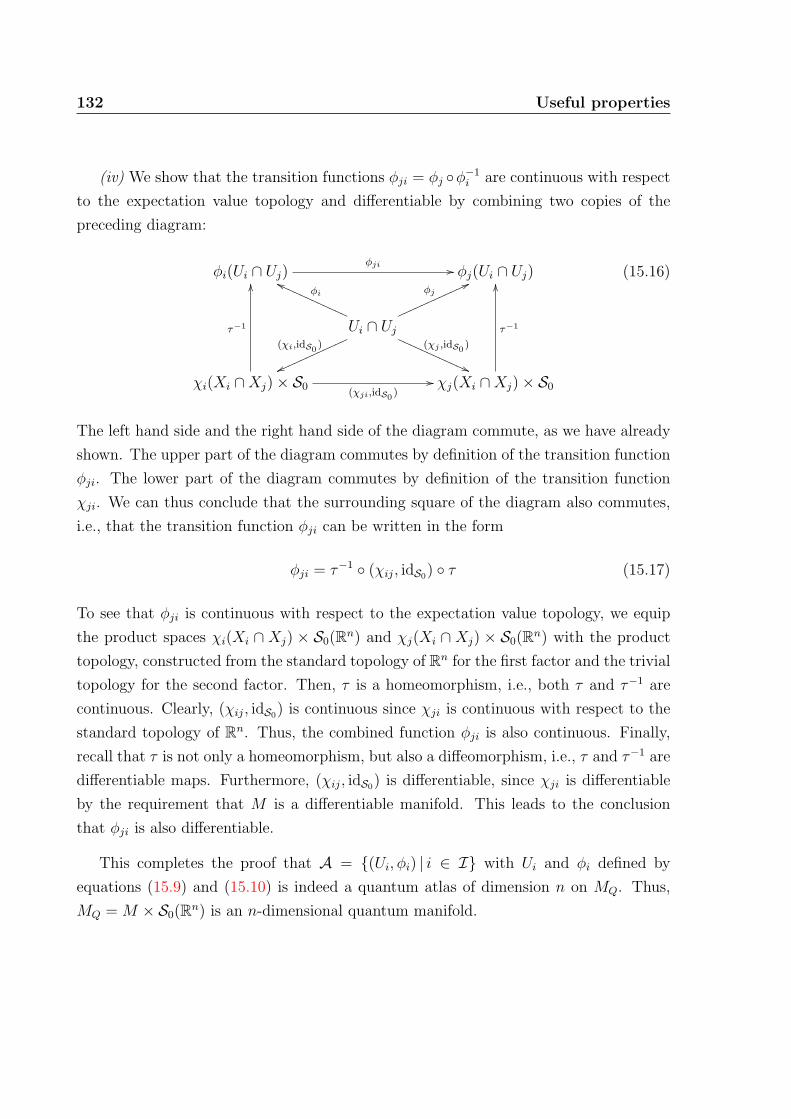
132 Useful properties
(iv) We show that the transition functions φji = φj ◦φ−1i are continuous with respect
to the expectation value topology and differentiable by combining two copies of the
preceding diagram:
φi(Ui ∩ Uj)φji // φj(Ui ∩ Uj)
Ui ∩ Uj
φi
hhPPPPPPPPPPPP
φj
66nnnnnnnnnnnn
(χi,idS0)
vvnnnnnnnnnnnn (χj ,idS0)
((QQQQQQQQQQQQ
χi(Xi ∩Xj)× S0
τ−1
OO
(χji,idS0)
// χj(Xi ∩Xj)× S0
τ−1
OO(15.16)
The left hand side and the right hand side of the diagram commute, as we have already
shown. The upper part of the diagram commutes by definition of the transition function
φji. The lower part of the diagram commutes by definition of the transition function
χji. We can thus conclude that the surrounding square of the diagram also commutes,
i.e., that the transition function φji can be written in the form
φji = τ−1 ◦ (χij, idS0) ◦ τ (15.17)
To see that φji is continuous with respect to the expectation value topology, we equip
the product spaces χi(Xi ∩ Xj) × S0(Rn) and χj(Xi ∩ Xj) × S0(Rn) with the product
topology, constructed from the standard topology of Rn for the first factor and the trivial
topology for the second factor. Then, τ is a homeomorphism, i.e., both τ and τ−1 are
continuous. Clearly, (χij, idS0) is continuous since χji is continuous with respect to the
standard topology of Rn. Thus, the combined function φji is also continuous. Finally,
recall that τ is not only a homeomorphism, but also a diffeomorphism, i.e., τ and τ−1 are
differentiable maps. Furthermore, (χij, idS0) is differentiable, since χji is differentiable
by the requirement that M is a differentiable manifold. This leads to the conclusion
that φji is also differentiable.
This completes the proof that A = {(Ui, φi) | i ∈ I} with Ui and φi defined by
equations (15.9) and (15.10) is indeed a quantum atlas of dimension n on MQ. Thus,
MQ = M × S0(Rn) is an n-dimensional quantum manifold.

Useful properties 133
15.2.2 Classical limit of a trivial quantization
It remains to be shown that the classical manifold M can be re-obtained from its trivial
quantization MQ = M×S0(Rn) by taking the Kolmogorov quotient and that the classical
atlas that corresponds to the quantum atlas A defined above is the original atlas A on
M .
To construct the Kolmogorov quotient of MQ, let (ξ, g), (ξ′, g′) be two topologically
indistinguishable elements of M . Further, let (Ui, φi) ∈ A be a chart of MQ with
(ξ, g) ∈ Ui, which corresponds to a chart (Xi, χi) ∈ A. Since Ui is the pre-image under
φi of a subset of S 6=0(Rn), which is open in the expectation value topology, Ui is also open
in the induced topology on MQ. Thus, (ξ′, g′) ∈ Ui, since topologically indistinguishable
elements are contained in the same open sets. Since φi is a homeomorphism with respect
to the induced topology on MQ, the images φi(ξ, g) = Tχi(ξ)g and φi(ξ′, g′) = Tχi(ξ′)g
′ are
topologically indistinguishable, i.e., their position expectation values Q(Tχi(ξ)g) = χi(ξ)
and Q(Tχi(ξ′)g′) = χi(ξ
′) coincide. This is the case if ξ = ξ′, as χi is a bijection.
The equivalence class [(ξ, g)] of topologically indistinguishable elements thus contains
all elements (ξ′, g′), for which ξ = ξ′, i.e., [(ξ, g)] = ξ×S0(Rn). This allows us to identify
the equivalence classes of topologically indistinguishable elements of MQ with elements
of M , i.e., writing the Kolmogorov projection as
Q : MQ →M , (ξ, g) 7→ ξ . (15.18)
We still have to check that the topology on M induced by the Kolmogorov projection
is the same as the topology generated by the atlas A. This means we have to show that
any set X ⊂ M is open in the topology underlying the atlas A if and only if it is open
in the induced topology (which means its pre-image Q−1(X) under the Kolmogorov
projection Q is open in MQ).
The first implication, that open with respect to A implies open in the induced topol-
ogy follows from the continuity of Q. Indeed, we can show that Q is continuous on
each chart (Ui, φi) of the atlas A, which in turn proves the continuity of Q on the whole
quantum manifold MQ. Recall that within any chart (Ui, φi), the Kolmogorov quotient
can be written in the form Q = χ−1i ◦ Q ◦ φi. The maps χi and φi are homeomorphisms
by the definition of the topologies of M and MQ. The position expectation value Q is
continuous by the definition of the expectation value topology on S 6=0(Rn). Therefore,
the composition Q is continuous.

134 Useful properties
To prove the converse, we assume that X ⊂M is open in the induced topology, i.e.,
that Q−1(X) is open on MQ. We now show that every open set U ⊂MQ can be written
as U = Q−1(X) for some X ⊂ M which is open with respect to A. But then X = X,
which proves X is open with respect to A. So let U ⊂ MQ be open. Then we can use
the quantum atlas to write
U =⋃i∈I
U ∩ Ui =⋃i∈I
φ−1i (φi(U ∩ Ui)) (15.19)
Since φi is a homeomorphism, the set φi(U∩Ui) is open in the expectation value topology
of S 6=0(Rn), i.e., there exist an open set WUi ⊂ Rn, such that φi(U ∩ Ui) = Q−1(WU
i ).
We can thus rewrite U ∩ Ui as
U ∩ Ui = {(ξ, g) ∈ Ui | Q(φi(ξ, g)) ∈ WUi } = {(ξ, g) ∈ Ui |χi(ξ) ∈ WU
i }
= χ−1i (WU
i )× S0(Rn) = Q−1(χ−1i (WU
i )) ,(15.20)
using the definition of φi in the second step. Inserting this equation into the decompo-
sition of U above leads to
U =⋃i∈I
Q−1(χ−1i (WU
i )) = Q−1(⋃i∈I
χ−1i (WU
i )). (15.21)
From this equation we see that every open set U ⊂ MQ is the pre-image under Q of a
union of sets χ−1i (WU
i ) ⊂M , which are open in the topology generated by the atlas A.
Thus, every open set U ⊂MQ is the pre-image of an open set W ⊂M .
By the results of this section, we have established a one-to-one correspondence be-
tween differentiable manifolds and their trivial quantization which is a quantum mani-
fold. So the existence of quantum manifolds is ensured. However, it should be empha-
sized that quantum manifolds admit a much richer structure than that of a trivial fiber
bundle. They allow for non-trivial fibrations as does, in a classical analogy, the Mobius
strip which fibers non-trivially over the circle.

Chapter 16
Physical interpretation
In the previous chapters we have defined the notion of a quantum manifold as a purely
mathematical construction and derived some of its properties. We have shown that it
is locally homeomorphic to an appropriate Schwartz space, while its global structure is
related to a classical limit manifold. Since the aim of our construction is to construct a
new mathematical framework for a unified formulation of quantum theory and gravity,
we need a connection between the mathematical notion of a quantum manifold and well-
established physical concepts present in these two theories. In this chapter, we speculate
on possible connections of this type. In section 16.1 we discuss the quantization of
fields from a quantum manifold perspective. We argue that classical fields defined on
a quantum manifold might obtain quantum properties from the viewpoint of a classical
observer. In section 16.2 we turn our focus to quantum mechanics and discuss how
the quantum behaviour of a point particle may arise from classical mechanics on the
quantum manifold.
16.1 Quantization of fields
Probably the most intuitive application of the quantum manifold approach is the appli-
cation to field theory. Consider a classical field theory where the dynamical variable is
a set of fields Φ defined on some spacetime manifold M . The dynamics of this theory
is given by a set of (local) field equations, which are (local) differential equations of the
fields. These equations typically arise from the variation of an appropriate action.
The quantum manifold idea uses a different approach in order to obtain a quantum
135

136 Physical interpretation
theory. The fields are not considered as functions on a classical manifold M , but rather
as functions defined on a quantum manifold MQ. The dynamics of the fields are also
defined on the quantum manifold, by a similar set of field equations as in classical field
theory. A classical observer, however, cannot measure the field as a function of MQ,
but is restricted to measurements on the underlying classical manifold. This lack of
knowledge of the field as a function on MQ is the origin of quantum properties of this
approach.
One may ask which value of the field a classical observer measures at some point ξ ∈M of the classical manifold if the field Φ is defined as a function on the quantum manifold.
In order to answer this question, we need a prescription for quantum measurements of
fields. Since ξ is an element of the classical manifold M , while the field Φ is a function
on the quantum manifold MQ, it seems natural to investigate the relationship between
M and MQ, which is given by the Kolmogorov projection Q : MQ →M . The quantum
object, which corresponds to the spacetime point ξ ∈M , is the fiber Q−1(ξ) ⊂MQ. The
field Φ may have different values on Q−1(ξ), which may be seen as the possible outcomes
of a measurement of Φ at ξ. Performing the measurement may be seen as choosing a
point ψ ∈ Q−1(ξ) of the quantum manifold, at which the field value is taken. A classical
observer cannot choose this point at will, so performing the measurement at a classical
point ξ corresponds to randomly picking a point ψ ∈ Q−1(ξ).
If we measure the field at different points ξi ∈ M , or within some region X ⊂ M ,
this means that we randomly pick several elements of the quantum manifold, one for
each point of the classical manifold where the field is measured. If we take X to be the
whole manifold M , we thus have to choose a function Ψ : M →MQ, with the additional
property that Q ◦Ψ = idM . Such a function is a section of the quantum manifold MQ,
considered as a fiber bundle over the classical manifold M . We thus conclude that a
quantum measurement corresponds to a section of the quantum manifold.
It seems natural to ask whether there are sections that are more probable as outcomes
of measurements than others. We thus need a probability density on the space of sections.
A hint how such a probability density might be obtained comes from the theory of path
integrals, where the probability of a path is related to its classical action. Since a section
Ψ assigns a field value Φ(Ψ(ξ)) to each point ξ ∈M of spacetime, we may consider Φ◦Ψ
as a classical field defined on the classical manifold M and thus compute its classical
action S. The classical solutions could then be obtained as the sections Ψ for which the
action is stationary, whereas the quantum theory is obtained by assigning each section
a probability density proportional to exp(iS).

Physical interpretation 137
The major advantage of this approach to quantizing a classical field theory is its
background independence. This arises from the fact that none of the background de-
pendent quantization schemes needs to be applied to quantize the theory. Its quantum
properties are generated purely by the classical dynamics of a field theory on MQ. This
invites us to consider also the spacetime metric as a function on MQ rather than on M ,
and to re-formulate general relativity as a classical field theory on MQ. The classical
spacetime metric then would become the result of a quantum measurement, as we would
expect from a quantum theory of gravity.
16.2 Quantization of a point particle
In order to probe the spacetime metric of general relativity, one considers the trajec-
tories γ : R → M of pointlike test particles of negligible mass. These trajectories, or
worldlines, are geodesics of the spacetime metric. If we wish to formulate the dynamics
of test particles in the quantum manifold approach, we first have to ask ourselves, which
mathematical object represents the point particle and its worldline. A possible choice
for a quantum worldline might be a worldline in MQ, i.e., a function γ : R → MQ.
This approach is similar to the field theory construction mentioned above, since classical
spacetime is simply replaced by quantum spacetime. But the mathematical consequences
are quite different. In the field theory construction, we replaced the domain of the field,
whereas in this case we replace the values of the worldline. This allows us to project
the worldline onto the classical spacetime M , using the Kolmogorov projection Q. A
quantum worldline γ gives thus rise to a classical worldline Q ◦ γ.
The question arises how one can obtain quantum properties from this construction,
if a quantum worldline completely determines a classical worldline, independent of any
measurement. In order to address this question we once again need a prescription how
measurements are performed. The obvious dynamical property of a point particle is its
position. If we measure the position of the particle at a fixed time, i.e., within a time
slice of M , we fix one point ξ of its classical worldline, namely the intersection of the
classical worldline and the time slice. But this gives us only partial information about
the quantum worldline. Instead of fixing a point in MQ, it only fixes a fiber Q−1(ξ),
which is intersected by the quantum worldline. In general the dynamics of the worldline,
given by the geodesic equation on MQ, depends on its position along the fiber and is
thus hidden to the classical observer, in a similar way as the wave function of standard

138 Physical interpretation
quantum mechanics. By analogy, one may even consider the possibility that the process
of measurement alters the position of the particle along the fiber, so that the motion of
the particle is disturbed by the position measurement.
Another quantum manifold approach to the dynamics of test particles arises from
replacing each point of the classical worldline by a submanifold of MQ. This idea is
similar to the construction of the quantum manifold itself, where each point ξ of the
classical manifold is replaced by a fiber Q−1(ξ), which is a submanifold of MQ. In this
case, the dynamics of the theory may be given by a set of equations motion for the
submanifold, similar to the dynamics of classical strings or branes.
Again we have to ask ourselves for a formulation of the process of position measure-
ment. If we make a position measurement at a fixed time, i.e., fix a time slice, we also fix
a submanifold of MQ, which is the union of all fibers corresponding to spacetime points
within our time slice. If we look at the intersection of this manifold and the world-
line manifold and project it onto classical spacetime, we get a picture of the possible
outcomes of a position measurement.

Chapter 17
Discussion
Motivated by the ubiquity of function spaces in quantum mechanics and field theory
and by the phenomenal success of differentiable manifold geometry in gravity, we have
developed a mathematical framework for quantum manifolds in this part of the thesis.
Quantum manifolds are infinite-dimensional manifolds locally homeomorphic to an ap-
propriate space of Schwartz functions, and thus unify geometric formulation and the
prominence of function spaces.
Through the topological identification of quantum points, which are charted as func-
tions having the same position expectation value, we have been able to show that there
exists a natural way of obtaining a classical limit geometry from the quantum manifold.
This procedure is known as the Kolmogorov quotient, and we demonstrated that the
classical limit yields nothing else but a finite-dimensional differentiable manifold. The
existence of the classical limit inbuilt into our construction is an all-important feature
if the mathematical idea of the quantum manifold is to be applied to physical mod-
elling. It is difficult to imagine how any quantum geometry of spacetime could hope for
a successful interpretation without clarifying how to reobtain a classical differentiable
background.
We could prove that a quantum manifold has the structure of a fiber bundle over
its associated classical limit geometry. The projection is the topological identification
given by the Kolmogorov projection, and the typical fibers are charted as functions that
all map to zero position expectation value. Making use of their fibre bundle structure
we could also show the existence of quantum manifolds. Simple examples are in fact
given by finite-dimensional differentiable manifolds to which the typical fibers are all
139

140 Discussion
trivially attached. We call this process trivial quantization; the classical limit of a
trivial quantization returns the original manifold as one might expect. However, as
in the case of the non-trivially fibered Mobius strip in finite-dimensional differential
geometry, trivial fiber bundles cannot capture the full breadth of possible geometries of
a quantum manifold. In some sense a quantum manifold is the opposite of a discretized
manifold, by blowing up every classical point into a whole fiber of functions.
Though our motivation is physical, our work remains mathematical with the aim to
lay the foundations for a rather ambitious project: the proposal to investigate whether
physical theories formulated on the infinite-dimensional quantum manifold geometry
may appear as quantum theories over a finite-dimensional geometry. Several more in-
gredients, mathematical as well as physical, will be needed in order to make progress
along these lines. Most important on the mathematical side certainly is a clear under-
standing of tensor bundles over the quantum manifold and their precise relation to the
respective bundles over the classical limit geometry. On the physical side this will enable
us to start phenomenological model building. Independent of the mathematical interest,
the link of quantum manifolds to physics needs be a primary goal for future work.
Ending on a note of speculation, the model building could involve quantum observers
given by curves with frames attached on the quantum manifold. These might measure
the components of certain tensor fields over the quantum manifold, at least in theory. In
practice, any real measurement seems to be restricted to events on a classical manifold.
Since this manifold arises by projection as the classical limit, this means that a real
observer would only have access to partial information on the observed system. Once
the mathematical framework is extended, it will be interesting to investigate whether this
would lead to hidden variables problems, or to an appealing probabilistic or statistical
interpretation. We are confident that quantum manifolds will find application since they
incorporate what seems to be the most fundamental measurement available: position
measurement, not in the absolute, but in the modern relativistic sense, as position
coordinates embedded in the differential geometry of the classical limit manifold.
The current status of this research is foundational, and must now pose more ques-
tions than answers. Our work is a first step towards building a rigorous mathematical
background structure for spacetime. The promise of this framework, if field theory on
quantum spacetime could be interpreted as quantum theory on classical spacetime, is
that a simple gravity theory on the quantum manifold could yield an exciting proposal
for a theory of quantum gravity. So this idea could provide a new unified description of
field theory and gravity.

Conclusion and summary of the
thesis
In this thesis we presented two geometric theories constructed to overcome some of the
problematic aspects of general relativity. The first theory, multimetric repulsive gravity,
provides potential explanations for various astronomical observations such as the accel-
erating expansion of the universe, the formation of filament-like structures and voids,
and the local velocity anomaly. The second theory, quantum manifolds, is motivated as
a first step towards a new mathematical framework for quantum theories in arbitrary
curved spacetimes. Both theories provide numerous opportunities for future research.
We will now give an outlook on a few of these opportunities.
In chapter 10 we computed a subset of the PPN parameters for multimetric gravity
theories starting from the linearized equations of motion. We have shown that these
are compatible with values obtained from high-precision solar system measurements. It
appears natural to ask whether the same is true also for the remaining parameters that
cannot be obtained from the linearized equations. The determination of these parameters
would require a perturbative expansion of the equations of motion up to quadratic order
in the metric perturbations which is very involved for multimetric gravity theories, but
should be carried out in future work.
As we have argued in the same chapter, the PPN parameters of a multimetric gravity
theory split into two subsets: those governing the observable gravitational interaction
within each, in particular the visible, matter sector, and those governing the gravitational
interaction between different matter sectors. The first set of PPN parameters is fixed
by experiments within very narrow bounds and thus provides a restriction on the class
of multimetric gravity theories. The second set of PPN parameters is undetermined and
cannot be measured directly, i.e., by light deflection on dark masses or the motion of
dark test particles within the solar system. However, the PPN parameters are closely
141

142 Discussion
linked to the equations of motion and thus influence the dynamics of both dark and
visible masses.
An example for a physical situation where the mutual interaction between the differ-
ent matter sectors becomes important is structure formation. We have already shown
this in chapter 9, where we presented a simple simulation of structure formation in the
Newtonian limit of multimetric repulsive gravity. Using the post-Newtonian limit in-
stead would increase the accuracy of such simulations, mainly in dense regions such as
galaxy clusters. In order to increase the accuracy even further, one may replace the
Euler method of integration by higher order techniques such as the Runge-Kutta or
Adams-Stormer methods. As an advanced improvement, one may replace the equation
of state for dust matter by a more realistic one, such as a mixture containing dust and
radiation, or even interacting standard model matter. However, calculations of this type
easily exhaust the possibilities of our simple algorithm.
In order to overcome these limitations, more sophisticated algorithms are needed.
For example, instead of computing the gravitational field generated by each point mass
in the simulation separately, one may consider groups of point masses and compute
their joint gravitational field using a multipole approximation. Algorithms of this type
include the tree method [8] and the more advanced fast multipole method [47] which
takes advantage of the fact that nearby point masses are subject to a similar acceler-
ation caused by distant groups of point masses. Another possibility is to use a mean
field approach obtained by solving the Poisson equation on a lattice [52]. These so-
called particle-mesh algorithms require significantly less computing time, but become
inaccurate for distances below the lattice parameter. This problem can be solved by
combining both tree and particle-mesh methods, as implemented in the GADGET-2
simulation code [110]. Adapting this code to our multimetric gravity framework would
allow a drastic refinement of the results of our simulation shown in chapter 9. A com-
parison of the simulated structure formation and the observed large-scale structure of
the universe could then be used to determine the parameters of our cosmological model
presented in chapter 8, such as the radius a0 and density ρ0 at the big bounce or the
number N of standard model copies.
Already our simple model for structure formation has shown that filament-like struc-
tures similar to those formed by visible galaxies in our universe should exist for all matter
sectors. Because of the mutual repulsion between the different matter types, such dark
structures should be concentrated in the galactic voids. Although they cannot be ob-
served directly, they should in principle be detectable by their effect on light passing

Discussion 143
through voids. If the voids were simply empty, or filled with a homogeneous distribu-
tion of dark energy as in the ΛCDM model, light should pass through them without
any distortion. But if the voids were filled with non-homogeneous distributions of dark
standard model matter, a light distortion by negative gravitational lensing should in
principle be detectable. Further research could use data obtained from weak lensing
measurements [124] in order to map potential repulsive gravity sources in the galactic
voids.
Since we cannot easily determine the distribution of repulsive dark structures by
direct observation, one may ask whether already the homogeneous and isotropic cosmo-
logical background presented in chapter 8 leads to the prediction of measurable effects.
In a simple model, one may consider visible galaxies as perturbations of this solution,
where the density of visible matter is increased, and the density of all other types of
matter is decreased due to the mutual repulsion between the different matter types. A
test mass in the vicinity of a galaxy would then be affected by both the attractive grav-
itational force of the visible matter in the galaxy and the repulsive gravitational force
of the surrounding negative mass. Since both forces are directed towards the visible
galaxy, this would be observed as an apparent increase of its total mass. Quantitative
calculations should show whether this effect could be responsible for the observed light
deflection and galaxy rotation curves, both of which are conventionally explained by
dark matter.
On a smaller scale one may ask whether a dilute form of repulsive matter might also
be present in the interstellar medium within visible galaxies. By a similar argument as
stated above, the density of the repulsive matter would then be reduced in the vicinity
of stars. Applied to our solar system this would lead to an additional force directed
towards the sun acting on test bodies in the outer solar system. Further calculations
should show whether this effect might explain the observed deceleration of the Pioneer
probes.
The dynamics of stellar systems provides another opportunity for further research.
One of the predictions of general relativity is the emission of gravitational waves by ro-
tating, non-axially-symmetric mass distributions, such as binary stars. Although gravi-
tational waves have not yet been observed directly, observations of binary pulsars have
shown a drift in their orbital periods which can be explained by an energy loss due to
the emission of gravitational waves [127]. The same effect should be present also in mul-
timetric gravity. However, since each type of mass acts as a source for all metrics, one
should expect that a binary star emits gravitational radiation in all metric sectors, each
144 Discussion
of them transporting energy away from the binary system. The ratio between the orbital
energy loss and the observable gravitational wave intensity should thus be different. Cal-
culations of this ratio should be performed in order to obtain precise predictions, which
may soon be tested by the upcoming experiments searching for gravitational waves.
The research possibilities we mentioned so far have in common that they are closely
linked to astronomical observations and can thus be summarized under the keyword mul-
timetric phenomenology. They could be complemented by various research possibilities
focusing on the mathematical foundations of multimetric gravity. An obvious possibility
is the construction of exact solutions and their classification. We have already presented
a class of cosmological solutions for a homogeneous and isotropic universe in chapter 8.
Another exact solution of particular interest would be the static spherically symmetric
metric generated by a single point mass, corresponding to the Schwarzschild solution of
general relativity. This and other solutions should be calculated in future research.
As we have argued in chapter 10, the requirement of a PPN consistent theory with
forces of equal strength and opposite direction acting on test masses in the Newtonian
limit does not distinguish a single multimetric gravity theory. Hence it would be desirable
to find and establish further physical and mathematical principles in order to restrict the
class of multimetric theories. One mathematical idea to restrict possible gravitational
actions could be to enlarge the symmetry group. While we restricted to a discrete
exchange symmetry with respect to arbitrary permutations of the sectors, one could
think of establishing a continuous symmetry group that mixes the sectors.
Further research on mathematical foundations is also required for the quantum man-
ifold construction presented in the second part of our thesis. Most importantly, a con-
nection between tensor fields on the quantum manifold and on the classical manifold
is needed in order to understand how a quantum measurement of fields may arise. In
order to model quantum measurements by a probabilistic theory, a connection between
quantum manifolds and probability measures is required. Finally, one may ask whether
these structures can be related to geometric properties of a quantum manifold, given in
terms of a metric or a connection.
Besides these mathematical issues, a clear physical interpretation of our quantum
manifold construction is required. We already speculated on possible physical inter-
pretations in the contexts of both quantum field theory and quantum mechanics in
chapter 16. Further research should show whether these theories can be recovered in
the case of a flat Minkowski background. By a similar argument, classical field the-

Discussion 145
ory and classical mechanics on curved spacetime backgrounds should be recovered in
the converse limit in which quantum effects become negligible. Finally, considering the
dynamics of the metric itself, it should be examined whether general relativity can be
recovered in the classical limit, and whether the generic quantum manifold approach
yields a framework for quantizing gravity.
This conclusion can be summarized by saying that the two different geometric con-
structions presented in this thesis both provide potential solutions for several of the
problematic aspects of general relativity highlighted in the introduction. Future re-
search is necessary for understanding both the experimental consistency of our models
and their mathematical ingredients. Our work thus lays the foundation for a broad
variety of new research topics, and offers new insights into the nature of gravity.

146

Appendix
147


Appendix A
C source code used for structure
formation
In this appendix we display the complete source code for our simulation of structure
formation presented in chapter 9. A comprehensive explanation can be found in sec-
tion 9.2.
1 /* Repulsive gravity simulator
with periodic boundary conditions
and dynamic expansion.
*/
#include <math.h>
6 #include <stdio.h>
#include <stdlib.h>
#include <time.h>
// Number N of standard model copies.
11 #define MASSTYPES 4
// Number n of objects per standard model copy.
#define BODYCOUNT 16384
// Initial scale factor a0.
#define INISIZE 1.0
16 // Period ` of the periodic boundary conditions.
#define BOX 1.0
// Time step ∆t for the Euler integrator method.
149

150 C source code used for structure formation
#define TIMESTEP 0.0005
// Total number of time steps to compute.
21 #define MAXSIM 2000
// Number of steps before writing the positions into the output file.
#define OUTSTEP 1
// Positions of the point masses...
26 double x[MASSTYPES][BODYCOUNT][3];
// ...and their velocities.
double v[MASSTYPES][BODYCOUNT][3];
int main(int argc, char** argv)
31 {
// Some counters.
int i, i2, j, j2, k, n;
// Scale factor a, a2, a, Hubble parameter H = aa, mass M.
double a, a2, da, h, m;
36 // Variables used to store distances.
double r, r3, d[3];
// Output files for point mass positions and the scale factor.
FILE* out;
FILE* cra;
41 // Start time of the program (for CPU usage statistics).
time_t t0;
// Initialize random number generator.
srand(t0 = time(NULL));
46 for(i = 0; i < MASSTYPES; i++)
{
for(j = 0; j < BODYCOUNT; j++)
{
for(k = 0; k < 3; k++)
51 {
// Place point mass somewhere in the cubic region.
x[i][j][k] = BOX * (double)rand() / (double)RAND_MAX;

C source code used for structure formation 151
// Set initial velocity to 0.
56 v[i][j][k] = 0.0;
}
}
}
61 // Set scale factor close to the initial value...
a = 1.001 * INISIZE;
// ...where nM(a0`)3 = ρ0 = 3
(N−2)a20.
m = 3 * INISIZE * BOX * BOX * BOX / (MASSTYPES - 2) / BODYCOUNT;
66 // Display some information about the initial conditions.
printf("Initial radius: %e\n", a);
printf("Initial density: %e\n",
m * BODYCOUNT / (a * a * a) / (BOX * BOX * BOX));
printf("Mass per object: %e\n", m);
71 printf("Mean distance: %e\n",
pow(BODYCOUNT, 1.0 / 3.0) * a * BOX);
printf("Mean distance / Schwarzschild radius: %e\n",
pow(BODYCOUNT, 1.0 / 3.0) * a * BOX / m);
76 // Open output files for point mass positions...
out = fopen("positions.m", "w");
fprintf(out, "{");
// ...and scale factors.
cra = fopen("scales.m", "w");
81 fprintf(cra, "{");
for(n = 0; n <= MAXSIM; n++)
{
// Compute a2 for later use.
86 a2 = a * a;
// Compute a =√
1− N−23
nMa`3
.
da = sqrt(1 - (MASSTYPES - 2) * m * BODYCOUNT
/ a / (BOX * BOX * BOX) / 3);

152 C source code used for structure formation
// Compute Hubble parameter H = aa.
91 h = da / a;
// Print number of iteration, CPU time, a, a, H.
printf("Run %d after %d seconds: a = %1.3e, da = %1.3e, h = %1.3e\n",
n, (int)(time(NULL) - t0), a, da, h);
96 if(n % OUTSTEP == 0)
{
if(n > 0)
{
fprintf(out, ",\n");
101 fprintf(cra, ",\n");
}
// Output point mass positions.
fprintf(out, "{");
106 for(i = 0; i < MASSTYPES; i++)
{
if(i > 0)
fprintf(out, ", ");
fprintf(out, "{");
111 for(j = 0; j < BODYCOUNT; j++)
{
if(j > 0)
fprintf(out, ", ");
fprintf(out, "{%f, %f, %f}",
116 x[i][j][0] / BOX,
x[i][j][1] / BOX,
x[i][j][2] / BOX);
}
fprintf(out, "}");
121 }
fprintf(out, "}");
// Output a, a and H.
fprintf(cra, "{%f, %f, %f}", a, da, h);
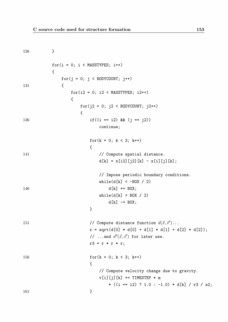
C source code used for structure formation 153
126 }
for(i = 0; i < MASSTYPES; i++)
{
for(j = 0; j < BODYCOUNT; j++)
131 {
for(i2 = 0; i2 < MASSTYPES; i2++)
{
for(j2 = 0; j2 < BODYCOUNT; j2++)
{
136 if((i == i2) && (j == j2))
continue;
for(k = 0; k < 3; k++)
{
141 // Compute spatial distance.
d[k] = x[i2][j2][k] - x[i][j][k];
// Impose periodic boundary conditions.
while(d[k] < -BOX / 2)
146 d[k] += BOX;
while(d[k] > BOX / 2)
d[k] -= BOX;
}
151 // Compute distance function d(~x, ~x′)...
r = sqrt(d[0] * d[0] + d[1] * d[1] + d[2] * d[2]);
// ...and d3(~x, ~x′) for later use.
r3 = r * r * r;
156 for(k = 0; k < 3; k++)
{
// Compute velocity change due to gravity.
v[i][j][k] += TIMESTEP * m
* ((i == i2) ? 1.0 : -1.0) * d[k] / r3 / a2;
161 }

154 C source code used for structure formation
}
}
}
}
166
for(i = 0; i < MASSTYPES; i++)
{
for(j = 0; j < BODYCOUNT; j++)
{
171 for(k = 0; k < 3; k++)
{
// Damping due to cosmological expansion.
v[i][j][k] -= TIMESTEP * v[i][j][k] * h;
176 // Advance the position of each point mass.
x[i][j][k] += TIMESTEP * v[i][j][k] / a;
// Periodic boundary conditions: 0 ≤ xα ≤ `.
while(x[i][j][k] < 0)
181 x[i][j][k] += BOX;
while(x[i][j][k] > BOX)
x[i][j][k] -= BOX;
}
}
186 }
// Increase a by ∆t · a.a += TIMESTEP * da;
}
191
// Close output files.
fprintf(out, "}");
fclose(out);
fprintf(cra, "}");
196 fclose(cra);

C source code used for structure formation 155
// Display some information about the final state.
printf("Final radius: %e\n", a);
printf("Final density: %e\n",
201 m * BODYCOUNT / (a * a * a) / (BOX * BOX * BOX));
printf("Mass per object: %e\n", m);
printf("Mean distance: %e\n", pow(BODYCOUNT, 1.0 / 3.0) * a * BOX);
printf("Mean distance / Schwarzschild radius: %e\n",
pow(BODYCOUNT, 1.0 / 3.0) * a * BOX / m);
206
return 0;
}

156

Appendix B
Coefficients of the linear PPN
ansatz
In this appendix we display the detailed expression for the coefficients c±1 , . . . , c±5 used in
the expansion of the geometry tensor given in equation (10.23). These can be computed
using the expression for the linearized geometry tensor (10.14) and the linearized PPN
metric ansatz (10.19):
c+1 = −(N+ +Q+)α+ − (N − 1)(N− +Q−)α−
+ (M+ + 3N+)γ+ + (N − 1)(M− + 3N−)γ−
− (M+ −N+)θ+ − (N − 1)(M− −N−)θ−
(B.1)
c−1 = −(N− +Q−)α+ − (N+ +Q+ + (N − 2)(N− +Q−))α−
+ (M− + 3N−)γ+ + (M+ + 3N+ + (N − 2)(M− + 3N−))γ−
− (M− −N−)θ+ − (M+ −N+ + (N − 2)(M− −N−))θ−
(B.2)
c+2 = Q+σ+
+ + (N − 1)Q−σ−+ (B.3)
c−2 = Q−σ++ + (Q+ + (N − 2)Q−)σ−+ (B.4)
157

158 Coefficients of the linear PPN ansatz
c+3 =
1
2
((P+ + 2R+)α+ + (N − 1)(P− + 2R−)α−
− (P+ + 6R+)γ+ − (N − 1)(P− + 6R−)γ−
+ (P+ − 2R+)θ+ + (N − 1)(P− − 2R−)θ−
+ (P+ + 2Q+)σ+− + (N − 1)(P− + 2Q−)σ−−
(B.5)
c−3 =1
2
((P− + 2R−)α+ + (P+ + 2R+ + (N − 2)(P− + 2R−))α−
− (P− + 6R−)γ+ − (P+ + 6R+ + (N − 2)(P− + 6R−))γ−
+ (P− − 2R−)θ+ + (P+ − 2R+ + (N − 2)(P− − 2R−))θ−
+ (P− + 2Q−)σ+− + (P+ + 2Q+ + (N − 2)(P− + 2Q−))σ−−
(B.6)
c+4 = N+α+ + (N − 1)N−α−
− (M+ + 3N+ +Q+)γ+ − (N − 1)(M− + 3N− +Q−)γ−
+ (M+ −N+ −Q+)θ+ + (N − 1)(M− −N− −Q−)θ−
(B.7)
c−4 = N−α+ + (N+ + (N − 2)N−)α−
− (M− + 3N− +Q−)γ+ − (M+ + 3N+ +Q+ + (N − 2)(M− + 3N− +Q−))γ−
+ (M− −N− −Q−)θ+ + (M+ −N+ −Q+ + (N − 2)(M− −N− −Q−))θ−
(B.8)
c+5 = R+α+ + (N − 1)R−α−
− (P+ + 3R+)γ+ − (N − 1)(P− + 3R−)γ−
+ (P+ + 2Q+ −R+)θ+ + (N − 1)(P− + 2Q− −R−)θ−
(B.9)
c−5 = R−α+ + (R+ + (N − 2)R−)α−
− (P− + 3R−)γ+ − (P+ + 3R+ + (N − 2)(P− + 3R−))γ−
+ (P− + 2Q− −R−)θ+ + (P+ + 2Q+ −R+ + (N − 2)(P− + 2Q− −R−))θ−
(B.10)

Appendix C
Technical proofs
In this appendix we include a number of proofs needed for the development of the results
in the main text. We will be concerned in turn with the continuity and differentiability
of the position expectation value map Q, with properties of the translation map T and
with the differentiability of the map τ and its inverse between the Schwartz space and
its corresponding trivial fibre bundle. As a matter of convenience, some proofs use the
nuclear, some the natural, topology on Schwartz space. Since these two are equivalent,
as discussed in section 13.3, the claims are true for both.
C.1 Continuity of the position expectation value
Claim 1. The position expectation value Q : S 6=0(Rn) → Rn defined in section 13.3 is
continuous with respect to the nuclear topology restricted to S 6=0(Rn) and the standard
topology on Rn.
Proof. Let W ⊂ Rn be open and V = Q−1(W ) ⊂ S 6=0. To show that V is open, we will
show that for all f0 ∈ V there exists an open set V ⊂ V containing f0. Since Q(f0) ∈ Wand W is open, there exists r > 0 and a corresponding open subset
WQ(f0),r := {x ∈ Rn | |x− Q(f0)| < r} ⊂ W . (C.1)
Now, in order to construct the sought-for open set V ⊂ Q−1(WQ(f0),r) ⊂ V , consider
159

160 Technical proofs
f ∈ S \ {−f0} and estimate
|Q(f0 + f)− Q(f0)| ≤ (| 〈f,Qf0〉 |+ | 〈f0,Qf〉 |+ | 〈f,Qf〉 |) ‖f0‖2
‖f0‖2‖f0 + f‖2
+(| 〈f0, f〉 |+ | 〈f, f0〉 |+ ‖f‖2) | 〈f0,Qf0〉 |
‖f0‖2‖f0 + f‖2,
(C.2)
using the definition of the expectation value and the triangular inequality. Choosing f
from a restricted open set of functions
V1 ={f ∈ S \ {−f0} | ‖f‖ <
1
2‖f0‖
}(C.3)
it follows that ‖f0 + f‖ > 12‖f0‖, so that we can remove f from the denominator of the
expression above. We also use the Cauchy-Schwartz inequality to bound all appearing
scalar products by norms, and the fact that
‖f‖ ≤ ‖f‖1 , ‖Qf‖ ≤ ‖f‖1 , (C.4)
where ‖f‖21 = 〈f, (Q2 + P 2 + 1)f〉, as defined in (13.12). This leads to
|Q(f0 + f)− Q(f0)| ≤ 4‖f‖1‖f0‖−3 [(‖Qf0‖+ ‖f0‖+ ‖f‖1) ‖f0‖+ ‖Qf0‖ (2‖f0‖+ ‖f‖1)] .
(C.5)
It is now clear that we can choose f from a further restricted function set V2 ⊂ V1 for
which ‖f‖1 is bounded above so that we achieve
|Q(f0 + f)− Q(f0)| < r (C.6)
for all f ∈ V2 = V1∩V2, which is open in the nuclear topology as the intersection of open
balls. Hence V := (V1 ∩V2) + f0 is open and V ⊂ Q−1(WQ(f0),r) ⊂ V . Since 0 ∈ V1 ∩V2,
we have f0 ∈ V . We have thus proven that every f0 ∈ V has an open neighborhood
V ⊂ V and thus V is open. So the pre-image V = Q−1(W ) of every open set W ⊂ Rn
is open, and Q continuous.
C.2 Differentiability of the position expectation value
Claim 2. The position expectation value Q : S 6=0(Rn)→ Rn is differentiable with respect
to the nuclear topology restricted to S 6=0(Rn) and the standard topology on Rn.

Technical proofs 161
Proof. According to the definition of differentiability in section 13.1, we have to show
that Q can be linearly approximated, more precisely, that for all f0 ∈ S 6=0 there exists
an open neighborhood V ⊂ S of 0 with −f0 /∈ V , a linear function DQ(f0) : S → Rn
and a tangent to zero δ : V → Rn such that for all f ∈ V
Q(f0 + f) = Q(f0) +DQ(f0)(f) + δ(f) . (C.7)
We first calculate the directional derivative d/dt|t=0(Q(f0 + tf)) to construct DQ(f0),
then we show that the remainder δ is indeed tangent to zero. Thus we find
DQ(f0)(f) =〈f0,Qf〉+ 〈f,Qf0〉 − Q(f0)(〈f0, f〉+ 〈f, f0〉)
〈f0, f0〉. (C.8)
We now show that δ defined by the two equations above is tangent to zero. In order
to do so, we follow similar steps as in the preceding section in obtaining an estimate
for δ(f). Employing the triangular inequality, the Cauchy-Schwartz inequality to bound
scalar products by norms, and the bounds (C.4) we arrive at
|δ(f)| ≤ 4‖f‖21‖f0‖−4
(3‖f0‖2 + 7‖f0‖‖Qf0‖+ ‖f0‖‖f‖1 + 3‖f‖1‖Qf0‖
)(C.9)
for all f in the same set V1 as defined by (C.3). We can now choose f from a further
restricted set V3 ⊂ V1 for which ‖f‖1 is bounded above in such a way that
|δ(tf)| < t2r (C.10)
for any given positive real r and |t| < 1. Note that V1 ∩ V3 is open as an intersection of
open balls. So δ maps all functions tf in the open set V1∩V3 into a ball Bt2r(0) ⊂ Rn of
radius t2r around the origin. Thus we can achieve δ(tf) ⊂ o(t)W with o(t) = t2 for any
open set W ⊂ Rn, proving that δ is tangent to zero, and Q differentiable as claimed.
C.3 Continuity of the translation operator
Aim of this section is to demonstrate the relevant continuity properties of the translation
operator T of Schwartz functions which was defined in section 15.1.1.
Claim 3. For all x ∈ Rn, the translation Tx : S(Rn)→ S(Rn), f 7→ Txf by x is a linear
homeomorphism with respect to the natural topology.

162 Technical proofs
Proof. Linearity of Tx simply follows from the definition of T , since for all λ ∈ R and
f, g in S(Rn):
Tx(λf) = (λf)(.− x) = λf(.− x) = λTxf , (C.11a)
Tx(f + g) = (f + g)(.− x) = f(.− x) + g(.− x) = Txf + Txg . (C.11b)
The inverse of Tx is given by T−x, so it is sufficient to show that Tx is continuous
and replace x by −x to show that the inverse is also continuous. By definition Tx is
continuous if for all open sets V ⊂ S the pre-image T−x(V ) is open, which is equivalent
to say that around every g0 ∈ T−x(V ) there exists an open neighborhood V ⊂ T−x(V ).
This is what we will now show.
Since V ⊂ S is open, there exists an r > 0 and a finite family of seminorms ‖.‖αj ,βj
for j = 1, . . . ,m so that
V ′ =m⋂j=1
V rαj ,βj
(Txg0) ⊂ V . (C.12)
For g ∈ S consider the expression
‖Tx(g0 + g)− Txg0‖αj ,βj= supy∈Rn
∣∣(yαjDβjg(y − x)
∣∣ = supy∈Rn
∣∣(x+ y)αjDβjg(y)
∣∣ .(C.13)
Expanding (x+ y)αj , and using the triangular inequality, it is easy to see that this can
be bounded by a sum over seminorms of lower length indices,
‖Tx(g0 + g)− Txg0‖αj ,βj≤
∑|γ|≤|αj |
C(αj ,γ,x)‖g‖αj−γ,βj , (C.14)
with positive coefficients C(αj ,γ,x) = C ′(αj ,γ)|xγ|. Choosing functions g in the open
set
m⋂j=1
⋂|γ|≤|αj |
Vrjαj−γ,βj (0) (C.15)
with all rj > 0 small enough, we achieve ‖Tx(g0 + g)− Txg0‖αj ,βj< r, and so (g0 + g) ∈

Technical proofs 163
T−x(V ′). It follows that the set defined by
V =m⋂j=1
⋂|γ|≤|αj |
Vrjαj−γ,βj (g0) (C.16)
is an open neighborhood of g0 and V ⊂ T−x(V ′) ⊂ T−x(V ), which completes the proof.
Claim 4. For all f ∈ S 6=0(Rn) the map Tf : Rn → S(Rn), x 7→ Txf is a continuous
injection with respect to the natural topology on S(Rn) and the standard topology on
Rn.
Proof. Obviously Txf 6= Tyf for all x 6= y and f ∈ S 6=0(Rn); hence Tf is injective. To
prove continuity, let V ⊂ S be open. We need to show that the pre-image (Tf)−1(V ) is
open. The empty set is always open, so assume x0 ∈ (Tf)−1(V ) 6= ∅. Since V is open,
there exists an r > 0 and a finite family of seminorms ‖.‖αj ,βjfor j = 1, . . . ,m such that
V ′ =m⋂j=1
V rαj ,βj
(Tx0f) ⊂ V . (C.17)
Define gj(y) = (x0 + y)αjDβjf(y) to rewrite
‖Tx0+x(f)− Tx0f‖αj ,βj= supy∈Rn
|gj(y − x)− gj(y)| = supy∈Rn
∣∣∣ ∫ y−x
y
dx · grad gj(x)∣∣∣
≤ supy∈Rn
(|x| sup
0≤t≤1|grad gj(y − tx)|
)≤ |x| sup
z∈Rn
|grad gj(z)| .
(C.18)
The right hand side exists, since f and so the gj are Schwartz functions. For any
given f we can choose x in an open ball Br(0) of sufficiently small radius r so that
‖Tx0+x(f) − Tx0f‖αj ,βj< r for all j. Then (x0 + x) ∈ (Tf)−1(V ′). It follows that the
open neighborhood Br(x0) of x0 satisfies Br(x0) ⊂ (Tf)−1(V ′) ⊂ (Tf)−1(V ). So we
conclude that (Tf)−1(V ) is open.
Claim 5. The translation operator T : Rn×S(Rn)→ S(Rn), (x, f) 7→ T (x, f) = Txf is
continuous with respect to the natural topology on S(Rn) and the corresponding product
topology on Rn × S(Rn).

164 Technical proofs
Proof. Let V ⊂ S be open and (x0, f0) ∈ T−1(V ). We will show that there exists an
open neighborhood Y ⊂ Rn×S of (x0, f0) such that Y ⊂ T−1(V ), which proves that the
pre-image T−1(V ) is open. Since V is open in the natural topology there exists r > 0
and a family of seminorms ‖.‖αj ,βjfor j = 1, . . . ,m so that
V ′ =m⋂j=1
V rαj ,βj
(T (x0, f0)) ⊂ V . (C.19)
Consider for x ∈ Rn and f ∈ S the expression
‖T (x0 + x, f0 + f)− T (x0, f0)‖αj ,βj≤ ‖T (x0 + x, f0 + f)− T (x0 + x, f0)‖αj ,βj
+ ‖T (x0 + x, f0)− T (x0, f0)‖αj ,βj.
(C.20)
The continuity of Tf0 proven in Claim 4 of this section tells us that we may find r > 0,
depending only on x0 and f0, so that for x ∈ Br(0) the second term becomes smaller
than r/2 for all j. A closer look at the proof of Claim 3 in this section reveals that the
first term can be made smaller than r/2 for all j by choosing f in a sufficiently small open
neighborhood of 0 given as a finite intersection of the form⋂V rkαk,βk
(0), where the rk again
only depend on x0 and f0. Combining these facts we obtain (x0 + x, f0 + f) ∈ T−1(V ′)
for (x, f) ∈ Br(0)×⋂V rkαk,βk
(0) which is open in the product topology. It follows that
Y =(Br(x0)×
⋂V rkαk,βk
(f0))⊂ T−1(V ′) ⊂ T−1(V ) (C.21)
is an open neighborhood, in the product topology, of (x0, f0), which completes the
proof.
C.4 Differentiability of τ and τ−1
We have shown in section 15.1.1 that the map τ : S 6=0(Rn) → Rn × S0(Rn) as defined
in (15.5) is a homeomorphism, making the model space S 6=0(Rn) of the quantum manifold
a trivial fibre bundle. Here we will show that τ is even a diffeomorphism.
Claim 6. The map τ is differentiable, with the natural topology on S(Rn). For all

Technical proofs 165
f0 ∈ S 6=0(Rn) the differential Dτ(f0) of τ at f0 is given by the linear map
Dτ(f0) : S(Rn) → Rn × S(Rn)
g 7→(DQ(f0)(g), DQ(f0)(g) · grad (T−Q(f0)f0) + T−Q(f0)g
) ,(C.22)
where the differential of Q is displayed in equation (C.8).
Proof. To prove this, we need to show that τ can be linearly approximated as
τ(f0 + f) = τ(f0) +Dτ(f0)(f) + δ(f) (C.23)
for all f in a small open neighborhood V ⊂ S of 0, and a tangent to zero δ defined on
V . We decompose δ(f) = (δ1(f), δ2(f)) ∈ Rn × S which gives
δ1(f) = Q(f0 + f)− Q(f0)−DQ(f0)(f) , (C.24)
δ2(f) = T−Q(f0+f)(f0 + f)− T−Q(f0)f0 −DQ(f0)(f) · grad T−Q(f0)f0 − T−Q(f0)f .
(C.25)
We already know from the proof of the differentiability of Q that δ1 is a tangent to zero.
To show that δ is a tangent to zero, it remains to show that δ2 is. To do so, we expand
δ2 as
δ2(f)(x) = f0(x+ Q(f0 + f))− f0(x+ Q(f0))−DQ(f0)(f) · grad f0(x+ Q(f0))
+ f(x+ Q(f0 + f))− f(x+ Q(f0)) .
(C.26)
Then we replace all occurrences of Q(f0 + f) using equation (C.24) and apply Taylor’s
theorem to the first term in each line, which yields
xαDβδ2(f)(x) = δ1(f) · grad xαDβf0(x+ Q(f0)) +∑|γ|=2
RxαDβf0γ (DQ(f0)(f) + δ1(f))γ
+ (DQ(f0)(f) + δ1(f)) · grad xαDβf(x+ Q(f0)) +∑|γ|=2
RxαDβfγ (DQ(f0)(f) + δ1(f))γ ,
(C.27)
where the sums involve only multiindices γ of length two, and the precise form of the
remainder terms RxαDβf0γ and R
xαDβfγ will not be required. Now choose an open neigh-
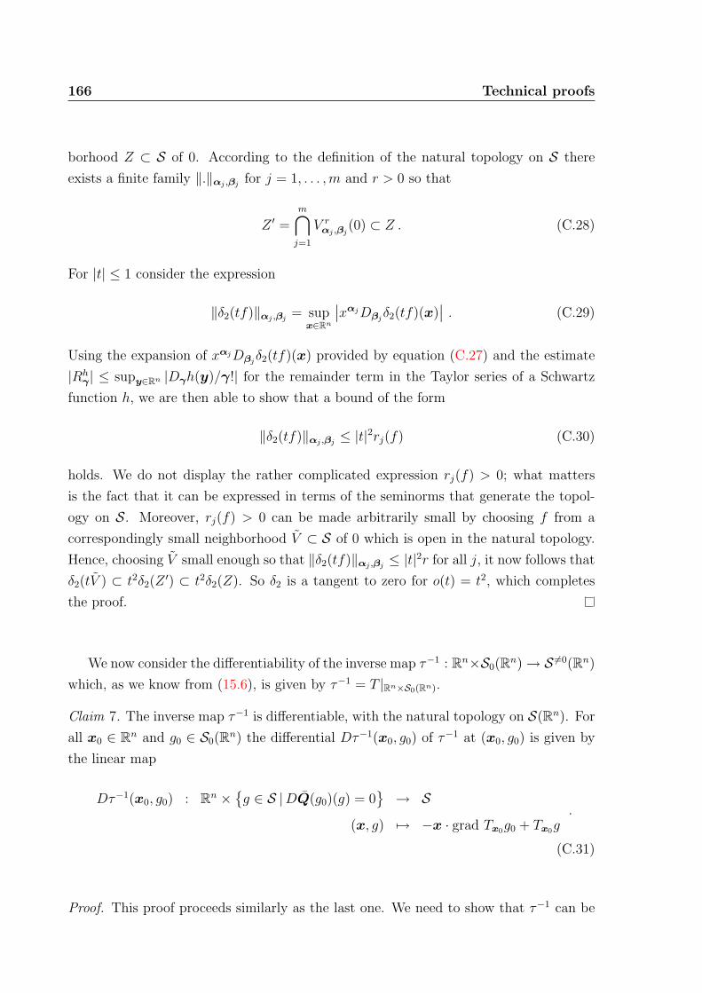
166 Technical proofs
borhood Z ⊂ S of 0. According to the definition of the natural topology on S there
exists a finite family ‖.‖αj ,βjfor j = 1, . . . ,m and r > 0 so that
Z ′ =m⋂j=1
V rαj ,βj
(0) ⊂ Z . (C.28)
For |t| ≤ 1 consider the expression
‖δ2(tf)‖αj ,βj= supx∈Rn
∣∣xαjDβjδ2(tf)(x)
∣∣ . (C.29)
Using the expansion of xαjDβjδ2(tf)(x) provided by equation (C.27) and the estimate
|Rhγ | ≤ supy∈Rn |Dγh(y)/γ!| for the remainder term in the Taylor series of a Schwartz
function h, we are then able to show that a bound of the form
‖δ2(tf)‖αj ,βj≤ |t|2rj(f) (C.30)
holds. We do not display the rather complicated expression rj(f) > 0; what matters
is the fact that it can be expressed in terms of the seminorms that generate the topol-
ogy on S. Moreover, rj(f) > 0 can be made arbitrarily small by choosing f from a
correspondingly small neighborhood V ⊂ S of 0 which is open in the natural topology.
Hence, choosing V small enough so that ‖δ2(tf)‖αj ,βj≤ |t|2r for all j, it now follows that
δ2(tV ) ⊂ t2δ2(Z ′) ⊂ t2δ2(Z). So δ2 is a tangent to zero for o(t) = t2, which completes
the proof.
We now consider the differentiability of the inverse map τ−1 : Rn×S0(Rn)→ S 6=0(Rn)
which, as we know from (15.6), is given by τ−1 = T |Rn×S0(Rn).
Claim 7. The inverse map τ−1 is differentiable, with the natural topology on S(Rn). For
all x0 ∈ Rn and g0 ∈ S0(Rn) the differential Dτ−1(x0, g0) of τ−1 at (x0, g0) is given by
the linear map
Dτ−1(x0, g0) : Rn ×{g ∈ S |DQ(g0)(g) = 0
}→ S
(x, g) 7→ −x · grad Tx0g0 + Tx0g.
(C.31)
Proof. This proof proceeds similarly as the last one. We need to show that τ−1 can be

Technical proofs 167
linearly approximated as
τ−1(x0 + x, g0 + g) = τ−1(x0, g0) +Dτ−1(x0, g0)(x, g) + δ(x, g) (C.32)
for all (x, g) in a sufficiently small open neighborhood V ⊂ (Rn × S) of (0, 0), and a
tangent to zero δ defined on V . From the definitions of τ−1 and T , we find
δ(x, g)(y) = g0(y − x0 − x)− g0(y − x0) + x · grad g0(y − x0)
+ g(y − x0 − x)− g(y − x0) .(C.33)
Application of Taylor’s theorem to the first term in each line yields
yαDβδ(x, g)(y) =∑|γ|=2
RyαDβg0γ xγ − x · grad yαDβg(y − x0) +
∑|γ|=2
RyαDβgγ xγ (C.34)
where, as above, the sums involve only multiindices γ of length two, and the precise
form of the remainder terms RxαDβf0γ and R
xαDβfγ will not be required. Now let S ⊂ S
be an open neighborhood of 0. There exists r > 0 and a finite family of seminorms
‖.‖αj ,βjfor j = 1, . . . ,m so that
S ′ =m⋂j=1
V rαj ,βj
(0) ⊂ S . (C.35)
We consider the expression
‖δ(tx, tg)‖αj ,βj= supy∈Rn
∣∣yαjDβjδ(tx, tg)(y)
∣∣ (C.36)
and employ the expansion of yαDβδ(x, g)(y) obtained above to show that the following
bound holds for ‖t‖ ≤ 1:
‖δ(tx, tg)‖αj ,βj|t|2(‖x‖ sup
y∈Rn
‖grad yαjβjg(y − x0)‖
+ ‖x‖2∑|γ|=2
supz∈Rn
1
γ!(|Dγ(yαjβjg0)|+ |Dγ(yαjβjg)|)
). (C.37)
It is clear that the term in brackets can be made smaller than r for all j by choosing
(x, g) from a sufficiently small set V ⊂ Rn × S, open in the relevant product topology.
It follows that δ(tV ) ⊂ t2S ′ ⊂ t2S, which shows that δ is a tangent to zero for o(t) = t2,
and hence τ−1 differentiable as claimed. For completeness, it is not hard to check that

168 Technical proofs
the differentials Dτ and Dτ−1 are inverses to one another.

Bibliography
[1] K. N. Abazajian et al. [ SDSS Collaboration ], Astrophys. J. Suppl. 182 (2009) 543
[arXiv:0812.0649 [astro-ph]].
[2] J. Ambjorn, J. Jurkiewicz and R. Loll, Phys. Rev. D 72 (2005) 064014 [arXiv:hep-
th/0505154].
[3] G. Amelino-Camelia, arXiv:0806.0339 [gr-qc].
[4] C. Armendariz-Picon, V. F. Mukhanov and P. J. Steinhardt, Phys. Rev. D 63
(2001) 103510 [arXiv:astro-ph/0006373].
[5] A. Ashtekar, Phys. Rev. Lett. 57 (1986) 2244.
[6] A. Ashtekar, M. Bojowald and J. Lewandowski, Adv. Theor. Math. Phys. 7 (2003)
233 [arXiv:gr-qc/0304074].
[7] J. M. Bardeen, Phys. Rev. D 22 (1980) 1882.
[8] J. Barnes, P. Hut, Nature 324 (1986) 446.
[9] D. F. Bartlett and D. Van Buren, Phys. Rev. Lett. 57 (1986) 21.
[10] J. D. Bekenstein, Phys. Rev. D 70, 083509 (2004) [Erratum-ibid. D 71, 069901
(2005)] [arXiv:astro-ph/0403694].
[11] J. D. Bekenstein, PoS JHW2004, 012 (2005) [arXiv:astro-ph/0412652].
[12] G. Bertone, D. Hooper and J. Silk, Phys. Rept. 405 (2005) 279 [arXiv:hep-
ph/0404175].
[13] J. J. van der Bij, H. van Dam and Y. J. Ng, Physica 116A (1982) 307.
[14] W. J. G. de Blok and A. Bosma, Astron. Astrophys. 385 (2002) 816 [astro-
ph/0201276].
169

170 Bibliography
[15] G. R. Blumenthal, S. M. Faber, J. R. Primack et al., Nature 311 (1984) 517.
[16] A. Bohm, Dirac kets, Gamow vectors and Gelfand triplets, Springer 1989.
[17] M. Bojowald, Phys. Rev. Lett. 86 (2001) 5227 [arXiv:gr-qc/0102069].
[18] L. Bombelli, J. H. Lee, D. Meyer and R. Sorkin, Phys. Rev. Lett. 59 (1987) 521.
[19] H. Bondi, Rev. Mod. Phys. 29 (1957) 423.
[20] N. Boulanger, T. Damour, L. Gualtieri et al., arXiv:hep-th/0009109.
[21] A. H. Chamseddine and A. Connes, J. Geom. Phys. 58 (2008) 38 [arXiv:0706.3688
[hep-th]].
[22] T. Chiba, T. Okabe and M. Yamaguchi, Phys. Rev. D 62 (2000) 023511 [arXiv:astro-
ph/9912463].
[23] R. Cirelli, A. Mania and L. Pizzocchero, J. Math. Phys. 31 (1990) 2891.
[24] R. Cirelli, A. Mania and L. Pizzocchero, J. Math. Phys. 31 (1990) 2898.
[25] M. Colless et al. [ The 2DFGRS Collaboration ], Mon. Not. Roy. Astron. Soc. 328
(2001) 1039 [astro-ph/0106498].
[26] A. Connes, Commun. Math. Phys. 182 (1996) 155 [arXiv:hep-th/9603053].
[27] F. I. Cooperstock and S. Tieu, Int. J. Mod. Phys. A22 (2007) 2293 [astro-
ph/0610370].
[28] E. J. Copeland, M. Sami and S. Tsujikawa, Int. J. Mod. Phys. D 15 (2006) 1753
[arXiv:hep-th/0603057].
[29] M. Davis, G. Efstathiou, C. S. Frenk and S. D. M. White, Astrophys. J. 292 (1985)
371.
[30] G. R. Dvali, G. Gabadadze and M. Porrati, Phys. Lett. B 485 (2000) 208 [arXiv:hep-
th/0005016].
[31] F. W. Dyson; A. S. Eddington and C. Davidson, Philos. Trans. Royal Soc. London
220A (1920) 291.
[32] A. Einstein, Ann. Physik 17 (1905) 891.

Bibliography 171
[33] A. Einstein, Jahrb. Radioakt. u. Elektronik 4 (1907) 411.
[34] A. Einstein, Ann. Physik 35 (1911) 898.
[35] A. Einstein, Sitzungsber. Preuss. Akad. Wiss. Berlin (Math. Phys.) 1915 (1915)
844.
[36] J. R. Ellis, J. S. Hagelin, D. V. Nanopoulos, K. A. Olive and M. Srednicki, Nucl.
Phys. B 238 (1984) 453.
[37] R. V. Eotvos, D. Pekar and E. Fekete, Ann. Physik 373 (1922) 11.
[38] A. Foppl, Sitzungsber. d. Kgl. Bayr. Akad. d. Wiss. 6 (1897) 93.
[39] A. Friedman, Zeitschr. f. Physik A 10 (1922) 377.
[40] G. Gamow, My World Line, Viking, New York 1970.
[41] G. W. Gibbons, Commun. Math. Phys. 35 (1974) 13.
[42] G. W. Gibbons, S. A. Hartnoll and A. Ishibashi, Prog. Theor. Phys. 113 (2005)
963 [arXiv:hep-th/0409307].
[43] F. Girelli, S. Liberati and L. Sindoni, Phys. Rev. D 75 (2007) 064015 [arXiv:gr-
qc/0611024].
[44] R. J. Gleiser and G. Dotti, Class. Quant. Grav. 23 (2006) 5063 [arXiv:gr-
qc/0604021].
[45] M. Grana, R. Minasian, M. Petrini and D. Waldram, arXiv:0807.4527 [hep-th].
[46] M. B. Green, J. H. Schwarz and E. Witten, Superstring Theory, Cambridge Uni-
versity Press 1987.
[47] L. Greengard and V. Rokhlin, J. Comput. Phys. 73 (1987) 325.
[48] M. Gualtieri, arXiv:math/0401221.
[49] D. Harari and C. Lousto, Phys. Rev. D 42 (1990) 2626.
[50] S. W. Hawking, Commun. Math. Phys. 43 (1975) 199.
[51] S. W. Hawking and W. Israel, 300 years of gravitation, Cambridge University Press
1987.

172 Bibliography
[52] R. W. Hockney and J. W. Eastwood, Computer Simulation Using Particles,
McGraw-Hill New York 1981.
[53] M. Hohmann, R. Punzi and M. N. R. Wohlfarth, arXiv:0809.3111 [math-ph].
[54] M. Hohmann and M. N. R. Wohlfarth, Phys. Rev. D 80 (2009) 104011
[arXiv:0908.3384 [gr-qc]].
[55] M. Hohmann and M. N. R. Wohlfarth, Phys. Rev. D 81 (2010) 104006
[arXiv:1003.1379 [gr-qc]].
[56] M. Hohmann, M. N. R. Wohlfarth, Phys. Rev. D 82 (2010) 084028 [arXiv:1007.4945
[gr-qc]].
[57] S. Hossenfelder, Phys. Lett. B636 (2006) 119. [arXiv:gr-qc/0508013].
[58] S. Hossenfelder, arXiv:gr-qc/0605083.
[59] E. Hubble, Proc. Nat. Acad. Sci. 15 (1929) 168.
[60] C. M. Hull, JHEP 0707 (2007) 079 [arXiv:hep-th/0701203].
[61] D. Huterer, M. S. Turner, Phys. Rev. D60 (1999) 081301 [arXiv:astro-ph/9808133].
[62] A. Y. Kamenshchik, U. Moschella and V. Pasquier, Phys. Lett. B 511 (2001) 265
[arXiv:gr-qc/0103004].
[63] T. W. B. Kibble, Commun. Math. Phys. 65 (1979) 189.
[64] E. Komatsu et al. [WMAP Collaboration], Astrophys. J. Suppl. 180 (2009) 330
[arXiv:0803.0547 [astro-ph]].
[65] L. B. Kreuzer, Phys. Rev. 169 (1968) 1007.
[66] A. A. Kryukov, Found. Phys. 34 (2004) 1225.
[67] A. A. Kryukov, Found. Phys. 36 (2006) 175 [arXiv:0704.3306 [quant-ph]].
[68] S. Lang, Differential manifolds, Addison-Wesley 1972.
[69] G. Lemaıtre, Ann. de la Soc. Sci. de Bruxelles A47 (1927) 49.
[70] H. A. Lorentz, Proc. Roy. Netherl. Acad. Art. Sci. 6 (1904) 809.
[71] A. Lue, Phys. Rept. 423 (2006) 1 [arXiv:astro-ph/0510068].

Bibliography 173
[72] K. A. Malik and D. Wands, Phys. Rept. 475 (2009) 1 [arXiv:0809.4944 [astro-ph]].
[73] R. B. Mann, Class. Quant. Grav. 14 (1997) 2927 [arXiv:gr-qc/9705007].
[74] P. D. Mannheim, Found. Phys. 30 (2000) 709 [arXiv:gr-qc/0001011].
[75] J. C. Maxwell, Phil. Trans. Roy. Soc. Lond. 155 (1865) 459.
[76] A. A. Michelson and E. W. Morley, Am. J. Sci. 34 (1887) 333.
[77] M. Milgrom, Astrophys. J. 270 (1983) 365.
[78] M. Milgrom, Astrophys. J. 306 (1986) 9.
[79] C. W. Misner, K. S. Thorne and J. A. Wheeler, Gravitation, Palgrave Macmillan
1973.
[80] J. W. Moffat, J. Math. Phys. 36 (1995) 3722 [Erratum-ibid. 36 (1995) 7128].
[81] M. Nakahara, Geometry, Topology and Physics, Institute of Physics Pub 2003.
[82] I. Newton, Philosophiæ Naturalis Principia Mathematica, 1687.
[83] H. Nicolai, K. Peeters and M. Zamaklar, Class. Quant. Grav. 22 (2005) R193
[arXiv:hep-th/0501114].
[84] J. Noldus and P. Van Esch, Phys. Lett. B 639 (2006) 667.
[85] K. Nordtvedt, Phys. Rev. 169 (1968) 1014.
[86] K. Nordtvedt, Phys. Rev. 169 (1968) 1017.
[87] B. Paczynski, Astrophys. J. 304 (1986) 1.
[88] P. J. E. Peebles, Large-Scale Structure of the Universe, Princeton University Press
1980.
[89] P. J. E. Peebles and B. Ratra, Astrophys. J. 325 (1988) L17.
[90] S. Perlmutter et al. [Supernova Cosmology Project Collaboration], Astrophys. J.
517 (1999) 565 [arXiv:astro-ph/9812133].
[91] J. Polchinski, String theory, Cambridge University Press 1998.
[92] J. Preskill, M. B. Wise and F. Wilczek, Phys. Lett. B 120 (1983) 127.

174 Bibliography
[93] G. Preti and F. de Felice, Am. J. Phys. 76 (2008) 671.
[94] R. Punzi, F. P. Schuller and M. N. R. Wohlfarth, Phys. Rev. D 76 (2007) 101501(R)
[arXiv:hep-th/0612133].
[95] R. Punzi, F. P. Schuller and M. N. R. Wohlfarth, JHEP 0702 (2007) 030 [arXiv:hep-
th/0612141].
[96] R. Punzi, F. P. Schuller and M. N. R. Wohlfarth, arXiv:0711.3771 [hep-th].
[97] B. Ratra and P. J. E. Peebles, Phys. Rev. D 37 (1988) 3406.
[98] R. D. Reasenberg, I. I. Shapiro, P. E. MacNeil et al., Astrophys. J. 234 (1979)
L219.
[99] M. Reed and B. Simon, Methods of modern mathematical physics, vol. 1, Academic
Press 1972.
[100] A. G. Riess et al. [Supernova Search Team Collaboration], Astron. J. 116 (1998)
1009 [arXiv:astro-ph/9805201].
[101] P. G. Roll, R. Krotkov and R. H. Dicke, Annals Phys. 26 (1964) 442.
[102] C. Rovelli, Quantum gravity, Cambridge University Press 2004.
[103] C. Rovelli, arXiv:0808.3505 [gr-qc].
[104] R. Ruffini and J. A. Wheeler, Physics Today 24 (1971) 30.
[105] F. P. Schuller and M. N. R. Wohlfarth, Phys. Lett. B 612 (2005) 93 [arXiv:gr-
qc/0411076].
[106] F. P. Schuller and M. N. R. Wohlfarth, JHEP 0602 (2006) 059 [arXiv:hep-
th/0511157].
[107] S. S. Shapiro, J. L. Davis, D. E. Lebach et al., Phys. Rev. Lett. 92 (2004) 121101.
[108] T. P. Sotiriou and V. Faraoni, arXiv:0805.1726 [gr-qc].
[109] M. Spivak, A Comprehensive Introduction to Differential Geometry, Publish or
Perish 1999.
[110] V. Springel, Mon. Not. Roy. Astron. Soc. 364 (2005) 1105. [arXiv:astro-
ph/0505010].

Bibliography 175
[111] V. Springel, S. D. M. White, A. Jenkins et al., Nature 435 (2005) 629.
[arXiv:astro-ph/0504097].
[112] J. M. Stewart, Class. Quant. Grav. 7 (1990) 1169.
[113] R. Sverdlov and L. Bombelli, arXiv:0801.0240 [gr-qc].
[114] T. Thiemann, arXiv:gr-qc/0110034.
[115] K. S. Thorne and C. M. Will, Astrophys. J. 163 (1971) 595, Astrophys. J. 163
(1971) 611, Astrophys. J. 169 (1971) 125.
[116] D. F. Torres, G. E. Romero and L. A. Anchordoqui, Mod. Phys. Lett. A 13 (1998)
1575 [arXiv:gr-qc/9805075].
[117] R. N. Treuhaft and S. T. Lowe, Astron. J. 102 (1991) 1879.
[118] R. B. Tully, arXiv:0708.0864 [astro-ph].
[119] R. B. Tully, arXiv:0708.2449 [astro-ph].
[120] R. B. Tully, E. J. Shaya and I. D. Karachentsev et al., Astrophys. J. 676 (2008)
184, [arXiv:0705.4139 [astro-ph]].
[121] S. G. Turyshev and V. T. Toth, [arXiv:1001.3686 [gr-qc]].
[122] G. Veneziano, Nuovo Cim. A57 (1968) 190.
[123] U. Le Verrier, Compt. rend. hebd. l’Acad. sci. 49 (1859) 379.
[124] L. Van Waerbeke and Y. Mellier, [arXiv:astro-ph/0305089].
[125] R. M. Wald, General Relativity, The University of Chicago Press 1984.
[126] J. Wambsganss, Living Rev. Rel. 1 (1998) 12. [arXiv:astro-ph/9812021].
[127] J. M. Weisberg and J. H. Taylor, Gen. Rel. Grav. 13 (1981) 1.
[128] H. Whitney, Ann. Math. 37 (1936) 645.
[129] C. M. Will, Astrophys. J. Lett. 393 (1992) L59.
[130] C. M. Will, Theory and experiment in gravitational physics, Cambridge University
Press 1993.

176 Bibliography
[131] C. M. Will, Living Rev. Rel. 9 (2005) 3 [arXiv:gr-qc/0510072].
[132] J. G. Williams, S. G. Turyshev and D. H. Boggs, Int. J. Mod. Phys. D 18 (2009)
1129 [arXiv:gr-qc/0507083].
[133] J. W. York, Ann. Inst. H. Poincare (A) 21 (1974) 319.
[134] M. Zabzine, arXiv:hep-th/0605148.
[135] F. Zwicky, Helv. Phys. Acta 6 (1933) 110.