Geometric Camera Calibration

Juho Kannala, Janne Heikkila and Sami S. Brandt

University of Oulu, Finland

January 7, 2008

Abstract

Geometric camera calibration is a prerequisite for making accurate geometricmeasurements from image data and it is hence a fundamental task in computervision. This article gives a discussion about the camera models and calibrationmethods used in the field. The emphasis is on conventional calibration methodswhere the parameters of the camera model are determined by using imagesof a calibration object whose geometric properties are known. The presentedtechniques are illustrated with real calibration examples where several differentkinds of cameras are calibrated using a planar calibration object.

1 Introduction

Geometric camera calibration is the process of determining geometric propertiesof a camera. Here the camera is considered as a ray-based sensing device andthe camera geometry defines how the observed rays of light are mapped ontothe image. The purpose of calibration is to discover the mapping between therays and image points. Hence, a calibrated camera can be used as a directionsensor where both the forward-projection and back-projection are known, i.e.,one may compute the image point corresponding to a given projection ray andvice versa.

The geometric calibration of a camera is usually performed by imaging acalibration object whose geometric properties are known. The calibration ob-ject often consists of one to three planes which contain visible control pointsin known positions. The calibration is achieved by fitting a camera model tothe observations which are the measured positions of the control points in thecalibration images. The camera model contains two kinds of parameters: theexternal parameters relate the camera orientation and position to the object co-ordinate frame and the internal parameters determine the projection from thecamera coordinate frame onto image coordinates. Typically, both the externaland internal camera parameters are estimated in the calibration process whichusually involves non-linear optimization and minimizes a suitable cost func-tion over the camera parameters. The sum of squared distances between themeasured and modeled control point projections is frequently used as the costfunction since it gives the maximum-likelihood parameter estimates assumingisotropic and independent normally distributed measurement errors.

1

Calibration by non-linear optimization requires a good initial guess for thecamera parameters. Hence, various methods have been proposed for the directestimation of the parameters. Most of these methods deal with conventionalperspective cameras but recently there has also been effort in developing modelsand calibration methods for more general cameras. In fact, the choice of asuitable camera model is an important issue in camera calibration. For example,the pinhole camera model, which is based on the ideal perspective projectionmodel and often used for conventional cameras, is not a suitable model foromnidirectional cameras which have a very large field of view. Hence, there hasbeen a recent trend towards generic calibration techniques which would allowthe calibration of various types of cameras.

In this article, we will provide an overview into geometric camera calibra-tion and its present state-of-the-art. However, since the literature for cameracalibration is vast and ever-evolving it is not possible to cover all the aspects indetail. Nevertheless, we hope that this article serves as an introduction to theliterature where more details can be found. The article is hence structured asfollows. First, in Section 2, we describe some historical background for cameracalibration. Thereafter we review different camera models with an emphasis oncentral cameras. After describing camera models we discuss methods for cameracalibration. The focus is on our previous works [1, 2]. Finally, in Section 5, wepresent some calibration examples with real cameras. The article is concludedin Section 6.

2 Background

Geometric camera calibration is a prerequisite for image-based metric 3D mea-surements and it has a long history in photogrammetry and computer vision.One of the first references is by Conrady [3] who derived an analytical expressionfor the geometric distortion in a decentered lens system. Conrady’s model fordecentering distortion was used by Brown [4] who proposed a plumb line methodfor calibrating radial and decentering distortion. Later on the approach usedby Brown was commonly adopted in photogrammetric camera calibration [5].

In photogrammetry, the emphasis has traditionally been in the rigorous ge-ometric modeling of the camera and optics. On the other hand, in computervision it is considered important that the calibration procedure is automatic andfast. For example, the well-known calibration method developed by Tsai [6] wasdesigned to be an automatic and efficient calibration technique for machine vi-sion metrology. This method uses a simpler camera model than [4] and avoidsthe full-scale non-linear search by using simplifying approximations. However,due to the increased processing power of personal computers the non-linear op-timization is not as time-consuming now as it was before. Hence, when thecalibration accuracy is important the camera parameters are usually refined bya full-scale non-linear optimization.

Besides increasing the theoretical understanding, the advances in geometriccomputer vision have also affected the practice of image-based 3D reconstructionduring the last two decades [7,8]. For example, while the traditional photogram-metric approach assumes a pre-calibrated camera, an alternative approach is tocompute a projective reconstruction with an uncalibrated perspective camera.The projective reconstruction is defined up to a 3D projective transformation

2

and it can be upgraded to a metric reconstruction by self-calibration [8]. Inself-calibration the camera parameters are determined without a calibrationobject; feature correspondences over multiple images are used instead. How-ever, the conventional calibration is typically more accurate and stable thanself-calibration. In fact, self-calibration methods are beyond the scope of thisarticle.

3 Camera models

In this section we describe several camera models which have appeared in theliterature. We concentrate on central cameras, i.e., cameras with a single effec-tive viewpoint. Single viewpoint means that all the rays of light arriving ontothe image travel through a single point in space.

3.1 Perspective cameras

The pinhole camera model is the most common camera model and it is a fair ap-proximation for most conventional cameras which obey the perspective model.Typically these conventional cameras have a small field of view (< 60◦). Thepinhole camera model is widely used and simple; essentially it is just a perspec-tive projection followed by an affine transformation in the image plane.

The pinhole camera geometry is illustrated in Fig. 1. In a pinhole camerathe projection rays meet at a single point which is the camera center C and itsdistance from the image plane is the focal length f . By similar triangles, it maybe seen in Fig. 1 that the point (Xc, Yc, Zc)

> in the camera coordinate frameis projected to the point (fXc/Zc, fYc/Zc)

> in the image coordinate frame. Interms of homogeneous coordinates this perspective projection can be representedby a 3 × 4 projection matrix,

xy1

'

f 0 0 00 f 0 00 0 1 0

Xc

Yc

Zc

1

where ' denotes equality up to scale.However, instead of the image coordinates (x, y)>, the pixel coordinates

(u, v)> are usually used and they are obtained by the affine transformation

(

uv

)

=

[

mu −mu cot α0 mv

sin α

] (

xy

)

+

(

u0

v0

)

, (1)

where (u0, v0)> is the principal point, α is the angle between u and v axis, and

mu and mv give the number of pixels per unit distance in u and v directions,respectively. The angle α is π

2in the conventional case of orthogonal pixel

coordinate axes.In practice, the 3D point is expressed in some world coordinate system that is

different from the camera coordinate system. The motion between these coordi-nate systems is given by a rotation R and translation t. Hence, in homogeneous

3

PSfrag replacements

α

C

O

m

X

p

xy

uv

X

Y

Z

Xc

Yc

Zc

image plane

principal axisf

R, t

Figure 1: Pinhole camera model. Here C is the camera center and the originof the camera coordinate frame. The principal point p is the origin of thenormalized image coordinate system (x, y). The pixel image coordinate systemis (u, v).

coordinates, the mapping of the 3D point X to its image m is given by

m '

mu −mu cot α u0

0 mv

sin αv0

0 0 1

f 0 0 00 f 0 00 0 1 0

[

R t

0 1

]

X

=

muf −muf cot α u0

0 mv

sin αf v0

0 0 1

[

R t]

X =

muf musf u0

0 muγf v0

0 0 1

[

R t]

X

(2)

where we have introduced the parameters γ = mv

mu sin αand s = − cot α in order

to simplify the notation. Since a change in the focal length and a change inthe pixel units are indistinguishable above we may set mu = 1 and write theprojection equation in the form

m ' K[

R t]

X, (3)

where the upper triangular matrix

K =

f sf u0

0 γf v0

0 0 1

(4)

is the camera calibration matrix and contains the five internal parameters of apinhole camera.

It follows from Eq. (3) that a general pinhole camera may be represented bya homogeneous 3 × 4 matrix

P = K[

R t]

(5)

4

which is called the camera projection matrix. If the left hand submatrix KR

is non-singular, as it is for perspective cameras, the camera P is called a finite

projective camera.A camera represented by an arbitrary homogeneous 3 × 4 matrix of rank 3

is called a general projective camera. This class covers the affine cameras whichhave a projection matrix whose last row is (0, 0, 0, 1) up to scale. A commonexample of an affine camera is the orthographic camera where the scene pointsare orthogonally projected onto the image plane.

3.1.1 Lens distortion

The pinhole camera is an idealized mathematical model for real cameras whichmay often deviate from the ideal perspective imaging model. Hence, the basicpinhole model is often accompanied with lens distortion models for more ac-curate calibration of real lens systems. The most important type of geometricdistortion is the radial distortion which causes an inward or outward displace-ment of a given image point from its ideal location. Decentering of lens elementscauses additional distortion which also has tangential components.

A commonly used model for lens distortion accounts for radial and decen-tering distortion [4,5]. According to this model the corrected image coordinatesx′, y′ are obtained by

x′ =x + x (κ1r2 + κ2r

4 + κ3r6 + . . .)

+(

ρ1(r2 + 2x2) + 2ρ2xy

) (

1 + ρ3r2 + . . .

)

y′ = y + y (κ1r2 + κ2r

4 + κ3r6 + . . .)

+(

2ρ1xy + ρ2(r2 + 2y2)

) (

1 + ρ3r2 + . . .

)

,

(6)

where x and y are the measured coordinates, and

x = x − xp

y = y − yp

r =√

(x − xp)2 + (y − yp)2.

Here the center of distortion (xp, yp) is a free parameter in addition to the radialdistortion coefficients κi and decentering distortion coefficients ρi. In the tradi-tional photogrammetric approach the values for the distortion parameters arecomputed by least-squares adjustment by requiring that images of straight linesare straight after the correction [4]. However, the problem with this approachis that not only the distortion coefficients but also the other camera parametersare initially unknown. For example, the formulation above requires that thescales in both coordinate directions are equal which is not the case with pixelcoordinates unless the pixels are square.

In [1] the distortion model of Eq. (6) was adapted and combined with thepinhole model in order to make a complete and accurate model for real cameras.This camera model has the form

m = P(X) = PX + C(PX), (7)

where P denotes the non-linear camera projection and P is the camera projec-tion matrix of a pinhole camera. The non-linear part C is the distortion model

5

PSfrag replacements

camera

orthographic

perspective

P

p

F

Z

F ′

mirror

parabolic

hyperbolic

elliptical

PSfrag replacements

camera

orthographic

perspective

P

p

F

Z

F ′

mirror

parabolic

hyperbolic

elliptical

PSfrag replacements

camera

orthographic

perspective

P

p

F

Z

F ′

mirror

parabolic

hyperbolic

elliptical

Figure 2: Central catadioptric camera with a hyperbolic, elliptical and parabolicmirror. The Z-axis is the optical axis of the camera and the axis of revolutionfor the mirror surface. The scene point P is imaged at p. In each case theviewpoint of the catadioptric system is the focal point of the mirror denotedby F . In the case of hyperbolic and elliptical mirrors the effective pinhole ofthe perspective camera must be placed at the other focal point which is heredenoted by F ′.

derived from Eq. (6). In [1], two parameters were used for both the radial anddecentering distortion, i.e. the parameters κ1, κ2 and ρ1, ρ2, and it was assumedthat the center of distortion coincides with the principal point of the pinholecamera.

3.2 Central omnidirectional cameras

Although the pinhole model accompanied with lens distortion models is a fairapproximation for most conventional cameras, it is not a suitable model foromnidirectional cameras whose field of view is over 180◦. This is due to the factthat, when the angle between the incoming light ray and the optical axis of thecamera approaches 90◦, the perspective projection maps the ray infinitely far inthe image and it is not possible to remove this singularity with the distortionmodel described above. Hence, more flexible models are needed and below wediscuss different models for central omnidirectional cameras.

3.2.1 Catadioptric cameras

In a catadioptric omnidirectional camera the wide field of view is achieved byplacing a mirror in front of the camera lens. In a central catadioptric camera theshape and configuration of the mirror are such that the complete catadioptricsystem has a single effective viewpoint. It has been shown that the mirrorsurfaces which produce a single viewpoint are surfaces of revolution whose two-dimensional profile is a conic section [9]. Practically useful mirror surfacesused in real central catadioptric cameras are planar, hyperbolic, elliptical andparabolic. However, a planar mirror does not change the field of view of thecamera [9].

The central catadioptric configurations with hyperbolic, elliptical and para-bolic mirrors are illustrated in Fig. 2. In order to satisfy the single viewpointconstraint the parabolic mirror is combined with an orthographic camera while

6

the other mirrors are combined with a perspective camera. In each case theeffective viewpoint of the catadioptric system is the focal point of the mirrordenoted by F in Fig. 2.

Single-viewpoint catadioptric image formation is well studied [9, 10] and ithas been shown that a central catadioptric projection, including the cases shownin Fig. 2, is equivalent to a two-step mapping via the unit sphere [10, 11]. Asdescribed in [11, 12], the unifying model for central catadioptric cameras maybe represented by a composed function H ◦ F so that

m = (H ◦ F)(Φ), (8)

where Φ=(θ, ϕ)> defines the direction of the incoming light ray which is mappedto the image point m = (u, v, 1)>. Here F first projects the object point ontoa virtual image plane and then the planar projective transformation H mapsthe virtual image point to the observed image point m. The two-step map-ping F is illustrated in Fig. 3(a), where the object point X is first projected

to q =(

cos ϕ sin θ, sin ϕ sin θ, cos θ)>

on the unit sphere, whose center O isthe effective viewpoint of the camera. Thereafter the point q is perspectivelyprojected to x from another point Q so that the line determined by O and Q isperpendicular to the image plane. The distance l = |OQ| is a parameter of thecatadioptric camera.

Mathematically the function F has the form

x = F(Φ) = r(θ)

(

cos ϕsin ϕ

)

, (9)

where the function r is the radial projection which does not depend on ϕ dueto radial symmetry. The precise form of r as a function of θ is determined bythe parameter l, i.e.,

r =(l + 1) sin θ

l + cos θ. (10)

This follows from the fact that the corresponding sides of similar triangles musthave the same ratio, thus r

sin θ= l+1

l+cos θ, as Fig. 3(a) illustrates.

In a central catadioptric system with a hyperbolic or elliptical mirror thecamera axis does not have to be aligned with the mirror symmetry axis. Thecamera can be rotated with respect to the mirror as long as the camera centeris at the focal point of the mirror. Hence, in the general case, the mappingH from the virtual image plane to the real image plane is a planar projectivetransformation [12]. However, often the axes of the camera and mirror areclose to collinear so that the mapping H can be approximated with an affinetransformation A [11]. That is,

m = A(x) = K

(

x

1

)

, (11)

where the upper triangular matrix K is defined in Eq. (4) and contains fiveparameters. (Here the affine transformation A has only five degrees of freedomsince we may always fix the camera coordinate frame so that the x-axis is parallelto the u-axis.)

7

PSfrag replacements

Q

O

xX

q

l

sin θ

cos θ

(12)

(10)

X

Zr

θ

π

2

(i)

(ii)

(iii)

(iv)

(v)

(a)

0 10

1

2

PSfrag replacements

Q

O

x

X

q

l

sin θ

cos θ(12)

(10)

X

Z

r

θπ

2

(i) (ii)(iii)

(iv)

(v)

(b)

Figure 3: (a) A generic model for a central catadioptric camera [11]. The Z-axis is the optical axis and the plane Z = 1 is the virtual image plane. Theobject point X is first projected to q on the unit sphere and thereafter q isperspectively projected to x from Q. (b) The projections of Eqs. (12)-(16).

3.2.2 Fish-eye lenses

Fish-eye cameras achieve a large field of view by using only lenses while thecatadioptric cameras use both mirrors and lenses. Fish-eye lenses are designedto cover the whole hemispherical field in front of the camera and the angle ofview is very large, possibly over 180◦. Since it is impossible to project thehemispherical field of view on a finite image plane by a perspective projectionthe fish-eye lenses are designed to obey some other projection model [13].

The perspective projection of a pinhole camera can be represented by theformula

r = tan θ (i. perspective projection), (12)

where θ is the angle between the principal axis and the incoming ray and r is thedistance between the image point and the principal point measured on a virtualimage plane which is placed at a unit distance from the pinhole. Fish-eye lensesinstead are usually designed to obey one of the following projections:

r = 2 tan(θ/2) (ii. stereographic projection), (13)

r = θ (iii. equidistance projection), (14)

r = 2 sin(θ/2) (iv. equisolid angle projection), (15)

r = sin(θ) (v. orthogonal projection), (16)

where the equidistance projection is perhaps the most common model. Thebehavior of the different projection models is illustrated in Fig. 3(b).

Although the central catadioptric cameras and fish-eye cameras have a dif-ferent physical construction they are not too different from the viewpoint ofmathematical modeling. In fact, the radial projection curves defined by Eq. (10)are quite similar to those shown in Fig. 3(b). In particular, when l=0 Eq. (10)defines the perspective projection, l=1 gives the stereographic projection (sincetan θ

2= sin θ

1+cos θ), and on the limit l → ∞ we obtain the orthogonal projection.

Hence, the problem of modeling radially symmetric central cameras is essentiallyreduced to modeling radial projection functions such as those in Fig. 3(b).

8

3.2.3 Generic model for central cameras

Here we describe a generic camera model which was proposed in [2] and issuitable for central omnidirectional cameras as well as for conventional cameras.As discussed above, the radially symmetric central cameras may be representedby Eq. (10) where the function F is given by Eq. (9). The radial projectionfunction r in F is an essential part of the model. If r is fixed to have the formof Eq. (12) then the model is reduced to the pinhole model. However, modelingof omnidirectional cameras requires a more flexible model and here we considerthe model

r = k1θ + k2θ3 + k3θ

5 + k4θ7 + k5θ

9 + . . . , (17)

which allows good approximation of all the projections in Fig. 3(b). In [2] it wasshown that the first five terms, up to the ninth power of θ, give enough degreesof freedom for accurate approximation of different projection curves. Hence, thegeneric camera model used here contains five parameters in the radial projectionfunction r.

However, real lenses may deviate from precise radial symmetry and, there-fore, the radially symmetric model above was supplemented with an asymmetricpart in [2]. Hence, instead of Eq. (10) the camera model proposed in [2] has theform

m = (A ◦ D ◦ F)(Φ), (18)

where D is the asymmetric distortion function so that D ◦F gives the distortedimage point xd which is then transformed to pixel coordinates by the affinetransformation A. In detail,

xd = (D ◦ F)(Φ) = r(θ)ur(ϕ) + ∆r(θ, ϕ)ur(ϕ) + ∆t(θ, ϕ)uϕ(ϕ), (19)

where ur(ϕ) and uϕ(ϕ) are the unit vectors in the radial and tangential direc-tions and

∆r(θ, ϕ)=(g1θ + g2θ3 + g3θ

5)(i1 cos ϕ + i2 sin ϕ + i3 cos 2ϕ + i4 sin 2ϕ), (20)

∆t(θ, ϕ)=(h1θ + h2θ3 + h3θ

5)(j1 cos ϕ + j2 sinϕ + j3 cos 2ϕ + j4 sin 2ϕ). (21)

Here both the radial and tangential distortion terms contain seven parameters.The asymmetric part in Eq. (19) models the imperfections in the optical

system in a somewhat similar manner as the distortion model in Section 3.1.1does. However, instead of rigorous modeling of optical distortions, here theaim is to provide a flexible mathematical distortion model that is just fitted toagree with the observations. This approach is often practical since there may beseveral possible sources of imperfections in the optical system and it is difficultto model all of them in detail.

The camera model defined above is denoted by M24 in the following sincethe number of parameters is 24: F and A have both 5 parameters and D has14 parameters. However, often it is assumed that the pixel coordinate system isorthogonal, i.e. s=0 in Eq. (4), so that the number of parameters in A is onlyfour. This model is denoted by M23. In addition, sometimes it may be useful toleave out the asymmetric part in order to avoid over-fitting. The correspondingradially symmetric models are here denoted by M9 and M6. The model M6

contains only two terms in Eq. (17) while M9 contains five.

9

3.2.4 Other distortion models

In addition to the camera models described in the previous sections there arealso several other models that have appeared in the literature. For example, theso called division model for radial distortion is defined by

r =rd

1 − c r2d

, (22)

where rd is the measured distance between the image point and the distortioncenter and r is the ideal undistorted distance [14, 15]. A positive value of thedistortion coefficient c corresponds to the typical case of barrel distortion [14].However, the division model is not suitable for cameras whose field of viewexceeds 180 degrees. Hence, other models must be used in this case and, forinstance, the two-parametric projection model

r =a −

√a2 − 4bθ2

2bθ(23)

has been used for fish-eye lenses [16]. Furthermore, a parameter-free methodfor determining the radial distortion was proposed in [17].

3.3 Non-central cameras

Most real cameras are strictly speaking non-central. For example, in the caseof parabolic mirror in Fig. 2 it is difficult to align the mirror axis and the axisof the camera precisely. Likewise, in the hyperbolic and elliptic configurations,the precise positioning of the optical center of the perspective camera in thefocal point of the mirror is practically infeasible. In addition, if the shape of themirror is not a conic section or the real cameras are not truly othographic orperspective the configuration is non-central. However, in practice the camera isusually negligibly small compared to the viewed region so that it is effectivelypoint-like. Hence, the central camera models are widely used and tenable inmost situations so that also here, in this article, we concentrate on centralcameras.

Still, there are some works where the single viewpoint constraint is relaxedand a non-central camera model is used. For example, a completely generic cam-era calibration approach was discussed in [18] and [19], where a non-parametriccamera model was used. In this model each pixel of the camera is associatedwith a ray in 3D and the task of calibration is to determine the coordinates ofthese rays in some local coordinate system. In addition, there has been workabout designing mirrors for non-central catadioptric systems that are compliantwith pre-defined requirements [20].

Finally, as a generalization of central cameras we would like to mention theaxial cameras where all the projection rays go through a single line in space [19].For example, a catadioptric camera consisting of a mirror and a central camerais an axial camera if the mirror is any surface of revolution and the cameracenter lies on the mirror axis of revolution. A central camera is a special caseof an axial camera. The equiangular [21, 22] and equiareal [23] catadioptriccameras are another classes of axial cameras. In equiareal cameras the projectionis area preserving whereas the equiangular mirrors are designed so that theradial distance measured from the center of symmetry in the image is linearlyproportional to the angle between the incoming ray and the optical axis.

10

4 Calibration methods

Camera calibration is the process of determining the parameters of the cameramodel. Here we consider conventional calibration techniques that use images of acalibration object which contains control points in known positions. The choiceof a suitable calibration algorithm depends on the camera model and below wedescribe methods for calibrating both perspective and omnidirectional centralcameras.

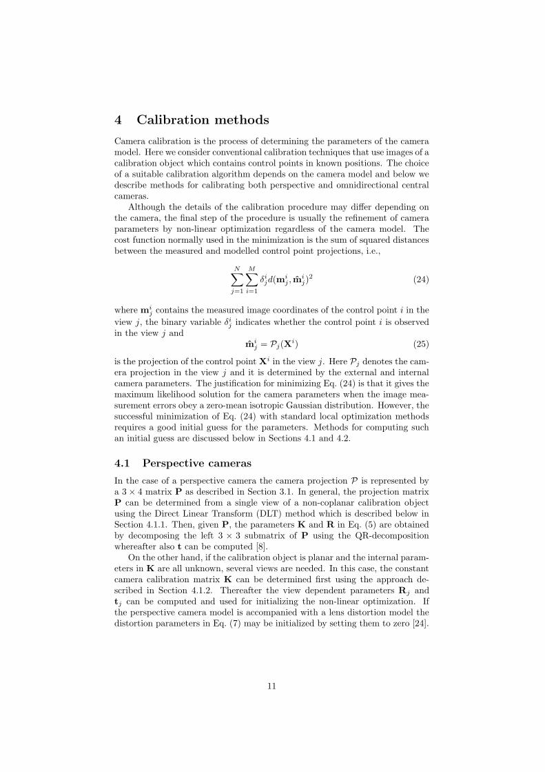
Although the details of the calibration procedure may differ depending onthe camera, the final step of the procedure is usually the refinement of cameraparameters by non-linear optimization regardless of the camera model. Thecost function normally used in the minimization is the sum of squared distancesbetween the measured and modelled control point projections, i.e.,

N∑

j=1

M∑

i=1

δijd(mi

j , mij)

2 (24)

where mij contains the measured image coordinates of the control point i in the

view j, the binary variable δij indicates whether the control point i is observed

in the view j andmi

j = Pj(Xi) (25)

is the projection of the control point Xi in the view j. Here Pj denotes the cam-era projection in the view j and it is determined by the external and internalcamera parameters. The justification for minimizing Eq. (24) is that it gives themaximum likelihood solution for the camera parameters when the image mea-surement errors obey a zero-mean isotropic Gaussian distribution. However, thesuccessful minimization of Eq. (24) with standard local optimization methodsrequires a good initial guess for the parameters. Methods for computing suchan initial guess are discussed below in Sections 4.1 and 4.2.

4.1 Perspective cameras

In the case of a perspective camera the camera projection P is represented bya 3 × 4 matrix P as described in Section 3.1. In general, the projection matrixP can be determined from a single view of a non-coplanar calibration objectusing the Direct Linear Transform (DLT) method which is described below inSection 4.1.1. Then, given P, the parameters K and R in Eq. (5) are obtainedby decomposing the left 3 × 3 submatrix of P using the QR-decompositionwhereafter also t can be computed [8].

On the other hand, if the calibration object is planar and the internal param-eters in K are all unknown, several views are needed. In this case, the constantcamera calibration matrix K can be determined first using the approach de-scribed in Section 4.1.2. Thereafter the view dependent parameters Rj andtj can be computed and used for initializing the non-linear optimization. Ifthe perspective camera model is accompanied with a lens distortion model thedistortion parameters in Eq. (7) may be initialized by setting them to zero [24].

11

4.1.1 Non-coplanar calibration object

Assuming that the known space points Xi are projected at the image pointsmi the unknown projection matrix P can be estimated using the DLT method[8, 25,26]. The projection equation gives

mi ' PXi, (26)

which can be written in the equivalent form

mi × PXi = 0, (27)

where the unknown scale in Eq. (26) is eliminated by the cross product. Theequations above are linear in the elements of P so they can be written in theform

Aiv = 0, (28)

where

v=(

P11 P12 P13 P14 P21 P22 P23 P24 P31 P32 P33 P34

)>(29)

and

Ai =

0> −mi3X

i> mi2X

i>

mi3X

i> 0> −mi1X

i>

−mi2X

i> mi1X

i> 0>

. (30)

Thus, each point correspondence provides three equations but only two of themare linearly independent. Hence, given M ≥ 6 point correspondences, we getan overdetermined set of equations Av = 0, where the matrix A is obtained bystacking the matrices Ai, i = 1, . . . ,M . In practice, due to the measurementerrors there is no exact solution to these equations but the solution v whichminimizes ||Av|| can be computed using the singular value decomposition ofA [8]. However, if the points Xi are coplanar ambiguous solutions exist for v

and hence the DLT method is not applicable in such case.The DLT method for solving P is a linear method which minimizes the

algebraic error ||Av|| instead of the geometric error in Eq. (24). This impliesthat, in the presence of noise, the estimation result depends on the coordinateframes where the points are expressed. In practice, it has been observed thata good idea is to normalize the coordinates in both mi and Xi so that theyhave zero mean and unit variance. This kind of normalization may significantlyimprove the estimation result in the presence of noise [8].

4.1.2 Planar calibration object

In the case of a planar calibration object the camera calibration matrix K canbe solved by using several views. This approach was described in [27] and [24]and it is briefly summarized in the following.

The mapping between a scene plane and its perspective image is a planarhomography. Since one may assume that the calibration plane is the planeZ = 0, the homography is defined by

m ' K[

R t]

XY01

= H

XY1

, (31)

12

where the 3 × 3 homography matrix

H = K[

r1 r2 t]

, (32)

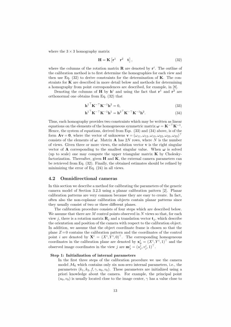
where the columns of the rotation matrix R are denoted by ri. The outline ofthe calibration method is to first determine the homographies for each view andthen use Eq. (32) to derive constraints for the determination of K. The con-straints for K are described in more detail below and methods for determininga homography from point correspondences are described, for example, in [8].

Denoting the columns of H by hi and using the fact that r1 and r2 areorthonormal one obtains from Eq. (32) that

h1>K−>K−1h2 = 0, (33)

h1>K−>K−1h1 = h2>K−>K−1h2. (34)

Thus, each homography provides two constraints which may be written as linearequations on the elements of the homogeneous symmetric matrix ω = K−>K−1.Hence, the system of equations, derived from Eqs. (33) and (34) above, is of theform Av = 0, where the vector of unknowns v = (ω11, ω12, ω13, ω22, ω23, ω33)

>

consists of the elements of ω. Matrix A has 2N rows, where N is the numberof views. Given three or more views, the solution vector v is the right singularvector of A corresponding to the smallest singular value. When ω is solved(up to scale) one may compute the upper triangular matrix K by Cholesky-factorization. Thereafter, given H and K, the external camera parameters canbe retrieved from Eq. (32). Finally, the obtained estimates should be refined byminimizing the error of Eq. (24) in all views.

4.2 Omnidirectional cameras

In this section we describe a method for calibrating the parameters of the genericcamera model of Section 3.2.3 using a planar calibration pattern [2]. Planarcalibration patterns are very common because they are easy to create. In fact,often also the non-coplanar calibration objects contain planar patterns sincethey usually consist of two or three different planes.

The calibration procedure consists of four steps which are described below.We assume that there are M control points observed in N views so that, for eachview j, there is a rotation matrix Rj and a translation vector tj , which describethe orientation and position of the camera with respect to the calibration object.In addition, we assume that the object coordinate frame is chosen so that theplane Z =0 contains the calibration pattern and the coordinates of the controlpoint i are denoted by Xi = (Xi, Y i, 0)>. The corresponding homogeneouscoordinates in the calibration plane are denoted by xi

p = (Xi, Y i, 1)> and the

observed image coordinates in the view j are mij = (ui

j , vij , 1)

>.

Step 1: Initialization of internal parameters

In the first three steps of the calibration procedure we use the cameramodel M6 which contains only six non-zero internal parameters, i.e., theparameters (k1, k2, f, γ, u0, v0). These parameters are initialized using apriori knowledge about the camera. For example, the principal point(u0, v0) is usually located close to the image center, γ has a value close to

13

1 and f is the focal length in pixels. The initial values for k1 and k2 canbe obtained by fitting the model r = k1θ + k2θ

3 to the desired projectioncurve in Fig. 3(b).

Step 2: Back-projection and computation of homographies

Given the internal parameters, we may back-project the observed pointsmi

j onto the unit sphere centered at the camera origin. For each mij the

back-projection gives the direction Φij = (θi

j , ϕij)

> and the points on the

unit sphere are defined by qij = (sin ϕi

j sin θij , cosϕi

j sin θij , cos θi

j)>. Since

the mapping between the points on the calibration plane and on the unitsphere is a central projection, there is a planar homography Hj so thatqi

j ' Hjxip. For each view j the homography Hj is estimated from the

correspondences (qij ,x

ip). In detail, the initial estimate for Hj is computed

by the linear algorithm [8] and it is then refined by minimizing∑

i sin2 αij ,

where αij is the angle between the unit vectors qi

j and Hjxip/||Hjx

ip||.

Step 3: Initialization of external parameters

The initial values for the external camera parameters are extracted fromthe homographies Hj . It holds that

qij '

[

Rj tj

]

Xi

Y i

01

=[

r1j r2

j tj

]

Xi

Y i

1

which implies Hj ' [r1j r2

j tj ]. Hence,

r1j = λjh

1j , r2

j = λjh2j , r3

j = r1j × r2

j , tj = λjh3j ,

where λj = ±||h1j ||−1. The sign of λj can be determined by requiring that

the camera is always on the front side of the calibration plane. However,the obtained rotation matrices may not be orthogonal due to estimationerrors. Hence, the singular value decomposition is used to compute theclosest orthogonal matrices in the sense of Frobenius norm which are thenused for initializing each Rj .

Step 4: Minimization of projection error

If a camera model with more than six parameters is used the additionalcamera parameters are initialized to zero at this stage. As we have theestimates for the internal and external camera parameters, we may com-pute the imaging function Pj for each camera, where a control point isprojected to mi

j = Pj(Xi). Finally, all the camera parameters are re-

fined by minimizing Eq. (24) using non-linear optimization, such as theLevenberg-Marquardt algorithm.

4.3 Precise calibration with circular control points

In order to achieve an accurate calibration, we have used a calibration plane withcircular control points since the centroids of the projected circles can be detectedwith a sub-pixel level of accuracy [28]. However, in this case the problem is thatthe centroid of the projected circle is not the image of the center of the originalcircle. Therefore, because mi

j in Eq. (24) is the measured centroid, we should not

14

project the centers as points mij since this may introduce bias in the estimates.

Of course, this is not an issue if the control points are really pointlike, such asthe corners of a checkerboard pattern.

In the case of a perspective camera the centroids of the projected circlescan be solved analytically given the camera parameters and the circles on thecalibration plane [1]. However, in the case of the generic camera model of Section3.2.3 the projection is more complicated and the centroids of the projected circlesmust be solved numerically [2].

5 Calibration examples

In this section, we illustrate camera calibration with real examples involvingdifferent kinds of cameras.

5.1 Conventional cameras with moderate lens distortion

The first calibrated camera was a Canon S1 IS digital camera with a zoom lenswhose focal length range is 5.8-58.0 mm which corresponds to a range of 38-380mm in the 35 mm film format. The calibration was performed with the zoomfixed to 11.2 mm. Hence, the diagonal field of view was about 30◦ which is arelatively narrow angle. The other camera was a Sony DFW-X710 digital videocamera equipped with a Cosmicar H416 wide-angle lens. The focal length ofthis wide-angle lens is 4.2 mm and it produces a diagonal field of view of about80◦.

Both cameras were calibrated by using a planar calibration pattern whichcontains white circles on black background. The pattern was displayed on adigital plasma display (Samsung PPM50M6HS) whose size is 1204 × 724mm2.A digital flat screen display provides a reasonably planar object and due toits self-illuminating property it is easy to avoid specular reflections which mightotherwise hamper the accurate localization of the control points. Some examplesof the calibration images are shown in Fig. 4. The image in Fig. 4(a) was takenwith the narrow-angle lens and the image in Fig. 4(b) with the wide-anglelens. The resolution of the images is 2048 × 1536 pixels and 1024 × 768 pixels,respectively. The lens distortion is clearly visible in the wide-angle image.

The number of calibration images was six for both cameras and each imagecontained 220 control points. The images were chosen so that the whole imagearea was covered by the control points. In addition to the set of calibrationimages we took another set of images which likewise contained six images wherethe control points were distributed onto the whole image area. These imageswere used as a test set in order to validate the results of calibration. In all casesthe control points were localized from the images by computing their gray-scalecentroids [28].

The cameras were calibrated using four different camera models. The firstmodel, denoted by Mp, was the skew-zero pinhole model accompanied with fourdistortion parameters. This model was used in [1] and it is described in Section3.1.1. The other three models were the models M6, M9 and M23 defined inSection 3.2.3. All the calibrations were performed by minimizing the sum ofsquared projection errors as described in Section 4. The computations were

15

carried out by using the publicly available implementations of the calibrationprocedures proposed in [1] and [2].1

The calibration results are shown in Table 1 where the first four rows givethe figures for the narrow-angle and wide-angle lenses introduced above. Thefirst and third row in Table 1 contain the RMS calibration errors, i.e., theroot-mean-squared distances between the measured and modeled control pointprojections in the calibration images. The second and fourth row show theRMS projection errors in the test images. In the test case the values of theinternal camera parameters were those estimated from the calibration imagesand only the external camera parameters were optimized by minimizing the sumof squared projection errors.

The results illustrate that the most flexible model M23 performs generallybest. However, the difference between the models M6, M9 and M23 is notlarge for the narrow-angle and wide-angle lens. The model Mp performs wellwith the narrow-angle lens but it seems that the other models are better inmodeling the severe radial distortion of the wide-angle lens. The relatively lowvalues of the test set error indicate that the risk of overfitting is small. This riskcould be further decreased by using more calibration images. The RMS erroris somewhat larger for the narrow-angle lens than for the wide-angle lens butthis may be due to the fact that the image resolution is higher in the narrow-angle case. Hence, the pixel units are not directly comparable for the differentcameras.

5.2 Omnidirectional cameras

We calibrated also a fish-eye lens camera and two different catadioptric cameras.The fish-eye lens which was used in the experiments is the ORIFL190-3 lensmanufactured by Omnitech Robotics. This lens has a 190◦ field of view andit was attached to a PointGrey Dragonfly color video camera, which has aresolution of 1024 × 768 pixels. The catadioptric cameras were constructed byplacing two different mirrors in front of the Canon S1 IS camera which has aresolution of 2048 × 1536 pixels. The first mirror was a hyperbolic mirror fromEizoh and the other mirror was an equiangular mirror from Kaidan. The field ofview provided by the hyperbolic mirror is such that when the mirror is placedabove the camera so that the optical axis is vertical the camera sees about30◦ above and 50◦ below the horizon (the region directly below the mirror isobscured by the camera). The equiangular mirror by Kaidan provides a slightlylarger view of field since it sees about 50◦ above and below the horizon. In theazimuthal direction the viewing angle is 360◦ for both mirrors.

Since the field of view of all the three omnidirectional cameras exceeds ahemisphere the calibration was not performed with the model Mp which isbased on the perspective projection model. Hence, we only report the resultsobtained with the central camera models M6, M9, and M23. The calibrationexperiments were done in a similar way as for the conventional cameras aboveand the same calibration object was used. However, here the number of imageswas 12 both in the calibration set and the test set. The number of images wasincreased in order to have a better coverage for the wider field of view.

The results are illustrated in Table 1 where it can be seen that the model

1http://www.ee.oulu.fi/mvg/page/downloads

16

Table 1: The RMS projection errors in pixels.

Mp M6 M9 M23

narrow-angle lens 0.293 0.339 0.325 0.280

test set error 0.249 0.309 0.259 0.236

wide-angle lens 0.908 0.078 0.077 0.067

test set error 0.823 0.089 0.088 0.088

fish-eye lens - 0.359 0.233 0.206

test set error - 0.437 0.168 0.187

hyperbolic mirror - 4.178 1.225 0.432

test set error - 3.708 1.094 0.392

equiangular mirror - 2.716 0.992 0.788

test set error - 3.129 1.065 0.984

M23 again shows best performance. The radially symmetric model M9 per-forms almost equally well with the fish-eye camera and the equiangular camera.However, for the hyperbolic camera the additional degrees of freedom in M23

clearly improve the calibration accuracy. This might be an indication that theoptical axis of the camera is not precisely aligned with the mirror axis. Neverthe-less, the asymmetric central camera model M23 provides a good approximationalso for this catadioptric camera. Likewise, here the central model seems to betenable also for the equiangular catadioptric camera which is strictly speakingnon-central. Note that the resolution of the fish-eye camera was different thanthat of the catadioptric cameras.

6 Conclusion

Geometric camera calibration is a prerequisite for image-based accurate 3Dmeasurements and it is therefore a fundamental task in computer vision andphotogrammetry. In this article we presented a review of calibration techniquesand camera models which commonly occur in applications. We concentrated onthe traditional calibration approach where the camera parameters are estimatedby using a calibration object whose geometry is known. The emphasis was oncentral camera models which are the most common in applications and providea reasonable approximation for a wide range of cameras. The process of cameracalibration was additionally demonstrated with practical examples where severaldifferent kinds of real cameras were calibrated.

Camera calibration is a wide topic and there is a lot of research which wasnot possible to be covered here. For example, recently there has been researchefforts towards completely generic camera calibration techniques which could beused for all kinds of cameras, also for the non-central ones. In addition, cameraself-calibration is an active research area which was not discussed in the scopeof this article. However, camera calibration using a calibration object and aparametric camera model, as discussed here, is the most viable approach whena high level of accuracy is required.

17

(a) (b)

(c) (d)

Figure 4: Images of the calibration pattern taken with different types of cameras.a) narrow-angle lens, b) wide-angle lens, c) fish-eye lens, d) hyperbolic mirrorcombined with a narrow-angle lens

References

[1] J. Heikkila, “Geometric camera calibration using circular control points,”IEEE Transactions on Pattern Analysis and Machine Intelligence, vol. 22,no. 10, pp. 1066–1077, 2000.

[2] J. Kannala and S. S. Brandt, “A generic camera model and calibrationmethod for conventional, wide-angle, and fish-eye lenses,” IEEE Transac-

tions on Pattern Analysis and Machine Intelligence, vol. 28, no. 8, pp.1335–1340, 2006.

[3] A. Conrady, “Decentering lens systems,” Monthly notices of the Royal As-

tronomical Society, vol. 79, pp. 384–390, 1919.

[4] D. C. Brown, “Close-range camera calibration,” Photogrammetric Engi-

neering, vol. 37, no. 8, pp. 855–866, 1971.

[5] C. C. Slama, Ed., Manual of Photogrammetry. Am. Soc. Photogrammetry,1980.

[6] R. Tsai, “A versatile camera calibration technique for high-accuracy 3Dmachine vision metrology using off-the-shelf TV cameras and lenses,” IEEE

Journal of Robotics and Automation, vol. RA-3, no. 4, pp. 323–344, 1987.

[7] O. Faugeras and Q.-T. Luong, The Geometry of Multiple Images. TheMIT Press, 2001.

18

[8] R. Hartley and A. Zisserman, Multiple View Geometry in Computer Vision,2nd ed. Cambridge, 2003.

[9] S. Baker and S. K. Nayar, “A theory of single-viewpoint catadioptric imageformation,” International Journal of Computer Vision, vol. 35, no. 2, 1999.

[10] C. Geyer and K. Daniilidis, “Catadioptric projective geometry,” Interna-

tional Journal of Computer Vision, vol. 45, no. 3, 2001.

[11] X. Ying and Z. Hu, “Catadioptric camera calibration using geometric in-variants,” IEEE Transactions on Pattern Analysis and Machine Intelli-

gence, vol. 26, no. 10, 2004.

[12] J. P. Barreto and H. Araujo, “Geometric properties of central catadioptricline images and their application in calibration,” IEEE Transactions on

Pattern Analysis and Machine Intelligence, vol. 27, no. 8, pp. 1327–1333,2005.

[13] K. Miyamoto, “Fish eye lens,” Journal of the Optical Society of America,vol. 54, no. 8, pp. 1060–1061, 1964.

[14] C. Brauer-Burchardt and K. Voss, “A new algorithm to correct fish-eye-and strong wide-angle-lens-distortion from single images,” in Proc. Inter-

national Conference on Image Processing, 2001.

[15] A. Fitzgibbon, “Simultaneous linear estimation of multiple view geometryand lens distortion,” in Proc. IEEE Conference on Computer Vision and

Pattern Recognition, 2001.

[16] B. Micusık and T. Pajdla, “Structure from motion with wide circular fieldof view cameras,” IEEE Transactions on Pattern Analysis and Machine

Intelligence, vol. 28, no. 7, 2006.

[17] R. Hartley and S. B. Kang, “Parameter-free radial distortion correctionwith center of distortion estimation,” IEEE Transactions on Pattern Anal-

ysis and Machine Intelligence, vol. 29, no. 8, pp. 1309–1321, 2008.

[18] M. D. Grossberg and S. K. Nayar, “A general imaging model and a methodfor finding its parameters,” in Proc. International Conference on Computer

Vision, 2001, pp. 108–115.

[19] S. Ramalingam, “Generic Imaging Models: Calibration and 3D Recon-struction Algorithms,” Ph.D. dissertation, Institut National Polytechniquede Grenoble, 2006.

[20] R. Swaminathan, M. D. Grossberg, and S. K. Nayar, “Designing mirror forcatadioptric systems that minimize image errors,” in Proc. Workshop on

Omnidirectional Vision, 2004.

[21] J. S. Chahl and M. V. Srinivasan, “Reflective surfaces for panoramic imag-ing,” Applied Optics, vol. 36, no. 31, pp. 8275–8285, 1997.

[22] M. Ollis, H. Herman, and S. Singh, “Analysis and design of panoramicstereo vision using equi-angular pixel cameras,” Carnegie Mellon Univer-sity,” CMU-RI-TR-99-04, 1999.

19

[23] R. A. Hicks and R. K. Perline, “Equi-areal catadioptric sensors,” in Proc.

Workshop on Omnidirectional Vision, 2002.

[24] Z. Zhang, “A flexible new technique for camera calibration,” IEEE Trans-

actions on Pattern Analysis and Machine Intelligence, vol. 22, no. 11, pp.1330–1334, 2000.

[25] Y. I. Abdel-Aziz and H. M. Karara, “Direct linear transformation fromcomparator to object space coordinates in close-range photogrammetry,”in Symposium on Close-Range Photogrammetry, 1971.

[26] I. Sutherland, “Three-dimensional data input by tablet,” in Proc. IEEE,vol. 62, 1974, pp. 453–461.

[27] P. Sturm and S. Maybank, “On plane based camera calibration: A gen-eral algorithm, singularities, applications,” in Proc. IEEE Conference on

Computer Vision and Pattern Recognition, 1999, pp. 432–437.

[28] J. Heikkila and O. Silven, “Calibration procedure for short focal lengthoff-the-shelf CCD cameras,” in Proc. International Conference on Pattern

Recognition, 1996, pp. 166–170.

20