Geographical patterns of community-based tree species...

1134

Spec

ial I

ssue

– C

ause

s an

d pa

tter

ns o

f div

ersi

ty in

Chi

na

Geographical patterns of community-based tree species richness in Chinese mountain forests: the effects of contemporary climate and regional history

Zehao Shen, Songlin Fei, Jianmeng Feng, Yining Liu, Zengli Liu, Zhiyao Tang, Xianping Wang, Xiaopu Wu, Chenyang Zheng, Biao Zhu and Jingyun Fang

Z. Shen ([email protected]), J. Feng, Y. Liu, Z. Liu, Z. Tang, X. Wang, X. Wu, C. Zheng, B. Zhu and J. Fang, Dept of Ecology, College of Urban and Environmental Sciences, and the Key Laboratory of Ministry of Education for Earth Surface Processes, Peking Univ., CN-100871 Beijing, PR China. – S. Fei, Dept of Forestry and Natural Resources, Purdue Univ., FORS 111, 195 Marsteller St., West Lafayette, IN 47907-2033, USA.

The relationship between climate/productivity and historical/regional contingency and their relative influence on geo-graphical patterns of species richness (GPSR) are still unresolved. Based on field data from 1494 plots from forests on 63 mountains across China, we document the GPSR for forest communities. Regression tree and generalized linear models were used to explore the discreteness and gradient of the distribution of tree species richness (a-diversity), and to estimate the correlations of climate, historical floristic region, and local habitat with species richness. The collinearity between climatic variables and region were further disentangled; and the spatial autocorrelation in the patterns of a-diversity and the residuals of alternative predictive models were compared. Overall, 75% of variation in plot-based a-diversity of trees was accounted for by all variables included, and about 66.5%, 64.5% and 27.9% by climate, region, and local habitat respectively. Importantly, the explanatory power of these variables differed in particular for coniferous, deciduous broa-dleaved and evergreen broadleaved species. Ambient temperature was more important for a-diversity of trees than were the other climatic variables across China. Spatial autocorrelation in the pattern of a-diversity could be accounted for mainly by spatial variation climate. The concordance between tree a-diversity, historical flora, contemporary climate, and Quaternary climate change mode suggests the climate/productivity and historical/regional contingency both contribute to the GPSR in a complimentary manner. Taken together, our results provide unique evidence to link of the effects of contemporary climate and historical climate change on species richness across scales.

Understanding geographical patterns of species richness (GPSR) and the underlying mechanisms has been a major topic in ecology and biogeography for more than a century (Brown and Gibson 1983, Hawkins 2004). A large body of empirical and theoretical studies have been conducted in the last decades, resulting in a well defined list of potential explanations (Willig et al. 2003, Field et al. 2008), centered on contemporary climate, regional/historical contingency and stochastic processes (Rohde 1992, Pimm and Brown 2004, Turner 2004). Even so, the contributions of these explanations to GPSR are quite variable across systems, and the integration of the various hypotheses into an explanatory framework is as of yet, incomplete (Ricklefs 2004, Ricklefs and Jenkins 2011, Rosindell et al. 2011).

The relative roles of contemporary climate/productivity and historical/regional contingency to GPSR have gener-ated strong debate in the literature. The climate/productivity hypothesis proposes a dominant effect of climate/productivity on GPSR, irrespective of the specific regional context (Wright 1983, Currie 1991, O’Brien et al. 2000, Francis and Currie

2003), whereas the regional/historical hypothesis argues for a significant contribution of unique regional and historical process on GPSR in additional to the effect of contempo-rary environment (Latham and Ricklefs 1993, Ricklefs 2004, Qian and Ricklefs 2004). Contemporary environ-mental factors are generally observed at ecological temporal scales and may reveal direct effects on local community processes, such as competition and ecological filtering (Currie 1991, Palmer 1994, Kerr and Packer 1997), whereas the effects of regional historical processes are found only at macro-scale, involving variation of speciation rate, extinc-tion rate or patterns of recolonization (Fang and Lechowicz 2006, Svenning and Skov 2007). Although empirical evidence has revealed a substantial amount of collinearity between the past and present (Ricklefs 1999, Hawkins et al. 2003a, b, Currie and Francis 2004, Svenning and Skov 2005, Field et al. 2008, Qian 2008, Wang et al. 2012), there is no consensus for their independent contri-butions, and efforts to integrate these two perspectives have begun to suggest a framework across a continuum of

Ecography 35: 1134–1146, 2012 doi: 10.1111/j.1600-0587.2012.00049.x

© 2013 The Authors. Ecography © 2013 Nordic Society Oikos Subject Editor: Nathan J. Sanders. Accepted 21 December 2012

1135

Special Issue – Causes and patterns of diversity in C

hina

spatiotemporal scales (Ricklefs 1987, 2004, 2008, White and Hurlbert 2010).

The scale (i.e. spatial extent and grain) of data is also critical for evaluating GPSR (Whittaker et al. 2001, Davies et al. 2007, Hurlbert and Jetz 2007). Richness of narrow ranged species tends to be more sensitive to habitat hetero-geneities at local scale, while the spatial patterns of broad-ranged species are often correlated well with the climatic gradient at larger spatial scales (Jetz and Rahbek 2002, Rahbek et al. 2007). On the other hand, the extent of the study area can reveal different patterns of species richness (Nogués-Bravo et al. 2008), and affect the relative contri-bution of different factors to the GPRS (Wang et al. 2009).

In general, there are two major approaches in GPSR studies, range-map based vs community based. The former overlays a collection of species range maps on a grid system to estimate species richness per grid in a given geographic region (Hurlbert and White 2005, LaSorte and Hawkins 2007). Most studies of this type address questions at regional to global extents, with a grain size mostly 10 km (Field et al. 2008). In contrast, community-based studies rarely focus on an area ~ 105 km2 or with plot sizes 0.1 ha. Thus, there is an obvious gap of scale-related information left between the two approaches, i.e. the macro-scale ( 105 km2, up to a continent) pattern of species richness with plot level ( 0.1 ha) information has rarely been provided (but see Wang et al. 2009, Lessard et al. 2011). As community-based data represent a measure-ment of a-diversity, instead of a potential (predicted) sum of local species richness and spatial species turnover across a much larger map grid, the pattern of community data thus provides an alternative test to particular biogeographic hypotheses, and would be critical in disentangling the contributions of the suite of potential factors on the GPSR.

China encompasses an area comparable to that of the USA or Europe but supports a significantly higher bio-diversity. This has been explained with reference to the USA in terms of its historical/regional features (Qian and Ricklefs 1999, 2000) as well as contemporary climate (Wang et al. 2011). Since all of these studies used the range map-based approach, a community-based analysis can provide complementary evidence for the pattern, and serve as a use-ful test of existing hypotheses. By depicting the three dimen-sional spatial pattern of a-diversity of tree species across China (excluding the Tibet-Qinghai Plateau, where the elevation is mostly above tree-line), and relating the patterns to spatial, climatic, historical/regional, and habitat factors, we aim to address the following questions: 1) what are the geographic patterns of a-diversity of tree species (i.e. the number of tree species in a local community) across China? 2) What are the main factors associated with the GPSR of the tree species? 3) How do the factors contribute differently to the GPRS of the specific taxonomic/ecological species groups and regions?

Material and methods

Field sampling and data collection

The survey of mountain forests followed a nested design, with a total of 1494 plots sampled on 63 mountains across

China (Fig. 1). For each mountain, plots were laid out along an elevation gradient, separated by a 50-m (sometimes 100 m) elevational interval between adjacent plots. Stands of non-native species were avoided. All plots were 20 30 m, comprising six 10 10 m subplots. In each plot, we measured the diameter at breast height (DBH) of all trees with DBH 3 cm. We sought to identify all species in the field, but specimens of unfamiliar species were brought back for later identification, with reference to the Flora of China (Wu et al. 2002–2012).

Species richness data

Species richness in each plot (which we use synonymously with a-diversity) was determined across all species and sepa-rately for coniferous, deciduous broadleaved and evergreen broadleaved species.

Environmental and spatial data

The plot-level environmental data were generated from four aspects, i.e. space, climate, historical floristic region and local habitat, as described with the following four variables.

SpaceGeographical coordinates (latitude, longitude, and eleva-tion) were recorded with GPS at the center of each plot. Space information was not used to describe the environment of the plots, but used to generate plot level climate data.

ClimateA group of climatic variables were generated for each plot through a set of well established predictive regression models fitted for China (Fang 1992, Wang 1996a, b). The regression models used latitude, longitude and elevation as predictors and were calibrated with long-term monitoring data (1950–2000) from 737 standardized meteorological stations across the country. For each plot, we first predicted the monthly mean temperature (MMT) and precipitation (MMP) with the climatic models, then calculated four categories of eco-climatic indices from the MMT and MMP data: 1) ambient energy (Turner et al. 1987): MAT – mean annual temperature; WI – warm index (annual sum of the mean monthly temperature above 5°C) (Prentice et al. 1992); ABT – annual biotic temperature (the sum of monthly temperature above 0°C, with values 30°C set to 30°C) (Holdridge 1947); 2) water–energy balance (Wright 1983): AET – annual actual evapotranspiration; 3) thermal season-ality and freezing limit (Carrara and Vázquez 2010): ART – annual range of monthly temperatures; MTCM – mean temperature of the coldest month; 4) precipitation and aridity: AP – annual precipitation; MI – moisture index (Thornthwaite and Hare 1955); SP – warmer semi-annual precipitation (from May to October); CVP – coefficient of variation of annual precipitation; PER – the ratio of potential evapor-transpiration to annual precipitation (see Fang et al. 2012 for detailed information on the calculation of these variables).

Historical floristic regionAccording a Neogene floristic regions map of China by Tao (1992) generated from pollen and fossil data, China

1136

Spec

ial I

ssue

– C

ause

s an

d pa

tter

ns o

f div

ersi

ty in

Chi

na

65°E

45°N

40°N

35°N

30°N

25°N

20°N

15°N

70°E 75°E 80°E 85°E 90°E 95°E 100°E 105°E 110°E 115°E 120°E 125°E 130°E 135°E 140°E

50°N

45°N

40°N

35°N

30°N

25°N

20°N

85°E 90°E 95°E 100°E 105°ELongitude (°)

Latit

ude

(°)

Legend

R1

R2

R3Species No.

DEM (m)152 – 300300 – 1500

1500 – 30003000 – 45004500 – 8685

1 ~ 34 ~ 67 ~ 10

11 ~ 2021 ~ 3031 ~ 4041 ~ 50

0 250 500 1000Km

110°E 115°E 120°E 125°E

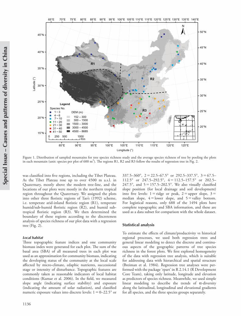
Figure 1. Distribution of sampled mountains for tree species richness study and the average species richness of tree by pooling the plots in each mountain (unit: species per plot of 600 m2). The regions R1, R2 and R3 follow the results of regression tree in Fig. 2.

was classified into five regions, including the Tibet Plateau. As the Tibet Plateau rose up to over 4500 m a.s.l. in Quaternary, mostly above the modern tree-line, and the locations of our plots were mostly in the northern tropical region throughout the Quaternary. We assigned the plots into other three floristic regions of Tao’s (1992) scheme, i.e. temperate arid-inland floristic region (R1), temperate humid/sub-humid floristic region (R2), and humid sub-tropical floristic region (R3). We then determined the boundary of these regions according to the discreteness analysis of species richness of our plot data with a regression tree (Fig. 2).

Local habitatThree topographic feature indices and one community biomass index were generated for each plot. The sum of the basal area (SBA) of all measured trees in each plot was used as an approximation for community biomass, indicating the developing status of the community at the local scale affected by micro-climate, edaphic nutrients, successional stage or intensity of disturbance. Topographic features are commonly taken as reasonable indicators of local habitat conditions (Kumar et al. 2006). In the field, we measured slope angle (indicating surface stability) and exposure (indicating the amount of solar radiation), and classified numeric exposure values into discrete levels: 1 0–22.5° or

337.5–360°, 2 22.5–67.5° or 292.5–337.5°, 3 67.5–112.5° or 247.5–292.5°, 4 112.5–157.5° or 202.5–247.5°, and 5 157.5–202.5°. We also visually classified slope position (for local drainage and soil development) into five levels: 1 ridge or peak, 2 upper slope, 3 median slope, 4 lower slope, and 5 valley bottom. For logistical reasons, only 688 of the 1494 plots have complete topographic and SBA information, and these are used as a data subset for comparison with the whole dataset.

Statistical analysis

To estimate the effects of climate/productivity vs historical regional processes, we used both regression trees and general linear modeling to detect the discrete and continu-ous aspects of the geographic patterns of tree species richness in the forest plots. We first explored homogeneity of the data with regression tree analysis, which is suitable for addressing data with hierarchical and spatial structure (Breiman et al. 1984). Regression tree analyses were per-formed with the package ‘rpart’ in R 2.14.1 (R Development Core Team), taking only latitude, longitude and elevation as predictors of species richness. Meanwhile, we used simple linear modeling to describe the trends of a-diversity along the latitudinal, longitudinal and elevational gradients for all species, and the three species groups separately.

1137


hina

component J resulting from the presence of collinearity among explanatory variables. For each variable, the inde-pendent and joint contributions are expressed as the per-centage of the total explained variance (R 2). The significance of the independent effect of each variable was determined by randomization (n 1000). Statistical significance was based on an upper confidence limit of 0.95 (Mac Nally 2002). We implemented this approach to plot-level overall tree species richness and by species group. We also com-pared models across the three historical regions. The HP procedure was performed using the package ‘hier.part’ (Walsh and Mac Nally 2007) in R. As this approach has a maximum upper limit of nine predictors, and including more variables will lead to estimation bias, we applied HP with ‘region’ plus eight top climatic variables chosen from the optimal GLM models, separately fitted for the species richness of all species or each of the species groups (Olea et al. 2010).

Results

Basic statistics of tree species richness

We recorded 2293 tree species with DBH 3 cm belonging to 117 families and 462 genera in the 1494 plots. There were 9 families, 22 genera and 82 species of conifers, and 108 families, 440 genera and 2211 species of broad-leaved spe-cies. The average a-diversity was 13.2 0.33 (mean SE) species per 600 m2 plot, including 1.0 0.03 conifer spe-cies, 4.7 0.22 evergreen broadleaved species, and 6.6 0.16 deciduous broadleaved species. The maximum a-diversity observed was 123 species in a tropical rainforest, and the minimum value was one species recorded in the

Following the suggestions in the recent discussion in the literature on spatial autocorrelation, that it is mostly too weak to really bias the estimate about the ecological relationships (Bini et al. 2009, Hawkins 2012), we did not generate spatially explicit regression models for species richness, but rather used a series of ordinary least squared (OLS) GLMs with climatic variables, local habitat factors (topography and biomass), and historical region as predic-tors. To satisfy the requirement of regression, the normality of all variables was checked, and non-normal distributed variables were log or square-root transformed depending on their original distribution. Stepwise procedures were used in combination with Akaike information criterion (AIC) value to select the best model, which has the lowest AIC value and optimal explained variations. These models were used to compare the effect of spatial, climatic, region and local hab-itat factors on plot-level tree species richness. We also fitted these models for the three tree species groups (conifers, evergreen broadleaf trees and deciduous broadleaf trees) to identify variable relationships with potential determinants.

To evaluate the potential impact of spatial autocorrela-tion on the models, we calculated spatial correlograms based on Moran’s I for the observed a-diversity values, and the residuals accounted for by the climate, region and local habitat models. The correlograms were generated in SAM ver. 4.0 (Rangel et al. 2010).

In order to estimate the independent effect of region to GPSR in addition to climate variables, it is critical to overcome the collinearity among variables (Leprieur et al. 2008), which we did using hierarchical variation partition-ing (HP) (Olea et al. 2010). The method addresses the collinearity issue by comparing models fitted with all possible subsets of predictors and estimating the indepen-dent influence I of each explanatory variable and the joint

Latitude > = 32.92°

Longitude < 102.09°

2.56 species n = 83

Elevation > = 2,619


1.60 species n = 16


7.24 species n = 132

Elevation > = 1,222



Elevation > = 2,695

Latitude > = 31.43° 8.50 species n = 93

24.29 species n = 479

14.44 speciesn = 105

Elevation > = 2,010



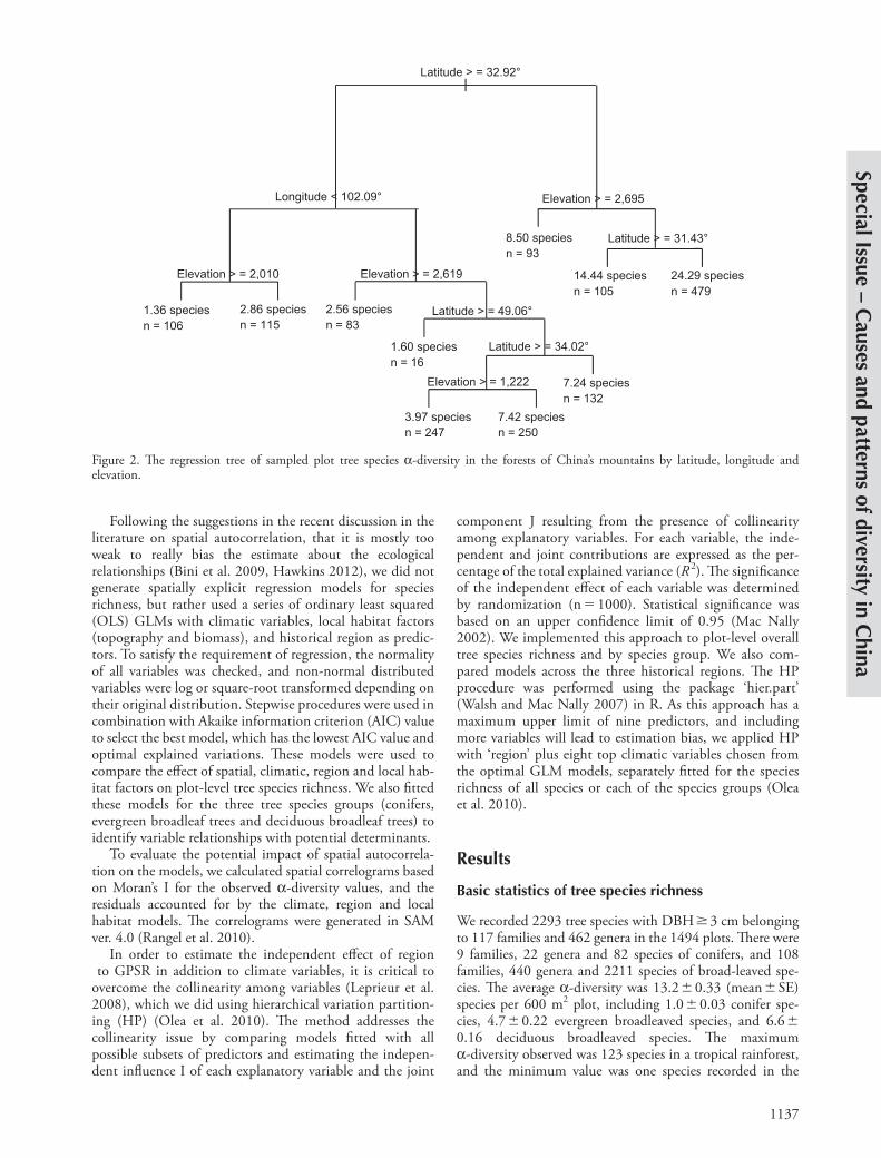
Figure 2. The regression tree of sampled plot tree species a-diversity in the forests of China’s mountains by latitude, longitude and elevation.

1138

Spec

ial I

ssue

– C

ause

s an

d pa

tter

ns o

f div

ersi

ty in

Chi

na

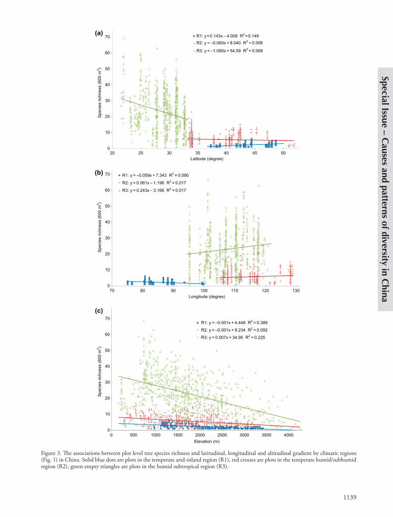
subtropical region (R3), the trend was much stronger (~ seven species/1000 m). Across all plots, the loss rate was 5.1 species/1000 m.

Effects of regional, climatic and habitat factors

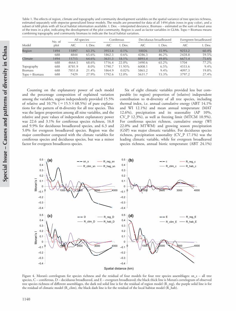
First of all, for each model (i.e. region, climate, etc.), the interpreted deviances (I.D.) of a-diversity are similar for the complete data set (all 1494 plots) and the subset (688 plots with habitat information) (Table 1). For all tree species and each of the three species groups, climate models had the highest explanatory power. Historical floristic region also accounted for a similar percentage of variation in a- diversity as the climate model (for all species), though it had almost no correlation with the pattern of coniferous spe-cies richness (I.D. 0.09%). In comparison, topographic variables and biomass played only a minor role in interpret-ing the GPSR of trees, and there was little overlap between the effects of topography and biomass.

The three species groups had different relationships with the various predictors. Species richness patterns for coniferous trees had the weakest correlation with all variables except for topography, whereas species richness of evergreen broadleaved trees had the strongest interpretation from all the determinants, except topography.

Moran’s I correlogram was applied to estimate spatial autocorrelation in a-diversity data and residuals of the climate, region and local habitat models (Fig. 4). For the observed data, there were two smaller scales (i.e. 74.9 and 727.9 km) of significant positive spatial autocorrela-tion (Moran’s I 0.2), and one scale (i.e. 2747.8 km) of significant negative spatial autocorrelation (Moran’s I 20.2). This pattern was similar for all tree species and for deciduous and evergreen broadleaved species, but there was no significant spatial autocorrelation at any scale for coniferous species richness. The spatial autocorrelation in observations of a-diversity was largely controlled in most of the models. The patterns of spatial autocorrelation for region, climate and local habitat models are comparable for both all species (Fig. 4a) and for conifers (Fig. 4b). For deciduous and evergreen broadleaved species, the climate model performed better in controlling spatial autocorrela-tion than did the region and local habitat model, especially at larger scales ( 2500 km). Therefore, the explanatory power of the models fitted with region, climate and local habitat variables were not significantly inflated by spatial autocorrelation, except for evergreen broadleaved species (Fig. 4d), which are mostly distributed in the subtropical region (R3). Here the region model had little effect in accounting for the spatial autocorrelation in residual, while the climate model had the best effect.

Hierarchical partitioning of variances

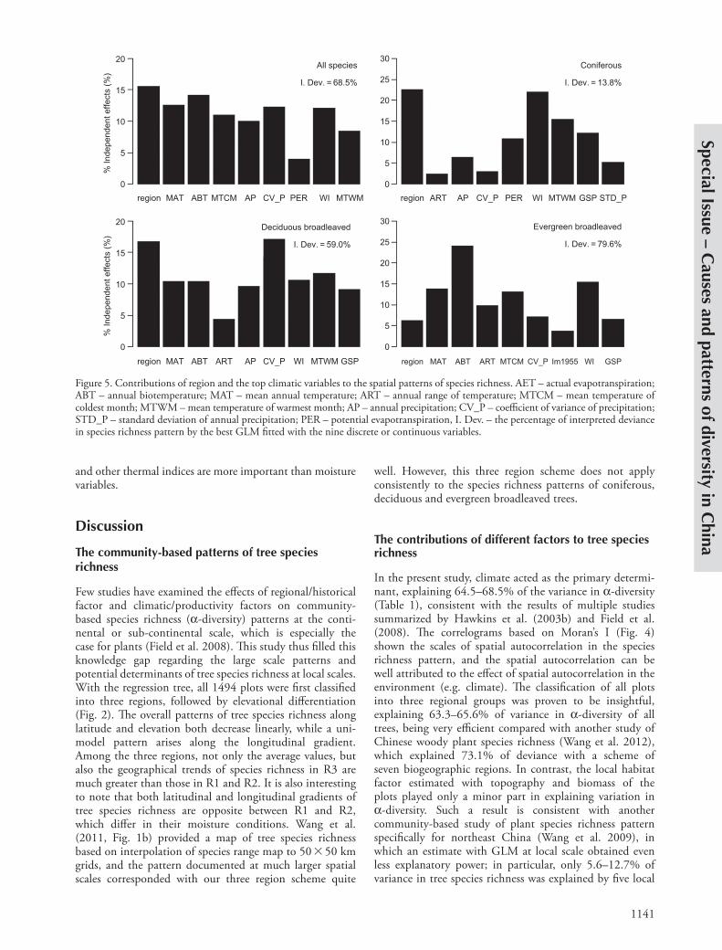
With the nine selected variables, the optimal model fitted with stepwise GLMs explained more than 68.5% of variance in a-diversity of all trees. In particular, this rate was 13.8, 59.0 and 79.6% for a-diversity of coniferous, deciduous broadleaved, and evergreen broadleaved species, respectively (Fig. 5).

alpine coniferous forests in the arid northwest. The fre-quency distribution of a-diversity was strongly left skewed for each category, with the median richness values as 8, 1, 5 and 0 species for all tree, coniferous, deciduous, and ever-green broadleaved species, respectively (Supplementary material Appendix 1, Fig. A1).

The geographic patterns of plot level tree species richness (a-diversity)

a-diversity of all trees was strongly associated with latitude, longitude and elevation. Regression tree analysis with three geographic coordinates generated a tree of 10 terminal branches, explaining 76.4% of the variance (Fig. 2). The first split represents latitude 32.9°N, accounting for 56.6% of all variance in a-diversity. Plots north of 32.9°N were further split by longitude 102.1°E, accounting for 7.1% of variance. Additional smaller groups were classified by elevation in the regression tree. As this spatial classifica-tion is in accord with that of the Tertiary floristic regions (Tao 1992), we pruned all plots in the regression tree into three groups, and the splitting coordinates were adopted as the borderlines between the three floristic regions, i.e. temperate arid-inland region (R1), temperate humid/ sub-humid region (R2), and humid subtropical region (R3).

R1: latitude 32.92, longitude 102.1, n 219, a- diversity (mean SE) 2.3 0.08 tree species per plot (600 m2).

R2: latitude 32.92, longitude 102.1, n 590, a-diversity 5.7 0.14 tree species per plot (600 m2).

R3: latitude 32.92, n 683, a-diversity 23.1 0.48 tree species per plot (600 m2).

a-diversity of trees was linearly correlated with latitude and elevation, overall and in each of the three regions. The tree richness patterns across longitudes were also linear within three regions but unimodel across all of them (Fig. 3). Specifically, a-diversity significantly decreased as latitude increased in the humid subtropical region (R3) or marginally significantly decreased in the temperate semi-humid region (R2), but increased with latitude in arid temperate inland China (R1). Across all 1494 plots, there was a stronger decreasing latitudinal trend of a- diversity of trees (rate 21.2 species degree21, r2 0.426, p 2.2 10216).

Along the longitudinal gradient (Fig. 3b), an overall uni-model pattern of a-diversity was comprised of low values in the two temperate regions (R1, R2) and a plateau of high values in the subtropical region of China (R3). There were significantly positive correlations between species richness and longitude in both R2 and R3 in the east, while an opposite trend was detected in the west (R1), indicating the lowest a-diversity occurred in the center of northern China.

The decline of a-diversity of tree species along the general elevation gradient was consistently significant across all three regions (Fig. 3c). In the northern part of China (R1 and R2), the elevational rate of the decrease in a- diversity was about one species/1000 m, whereas in the

1139


hina

70

60

50

40

R1: y = 0.143x – 4.008 R2 = 0.149R2: y = –0.060x + 8.040 R2 = 0.006

R3: y = –1.090x + 54.59 R2 = 0.068

30

20

10

0

70 R1: y = –0.059x + 7.343 R2 = 0.090

R2: y = 0.061x – 1.196 R2 = 0.017

R3: y = 0.243x – 3.166 R2 = 0.01760

50

40

30

20

10

0

20

70 80 90 100Longitude (degree)

110 120 130

25 30 35Latitude (degree)

Spec

ies

richn

ess

(600

m2 )

Spec

ies

richn

ess

(600

m2 )

70

60

50

40

30

20

10

00 500 1000 1500

Elevation (m)2000 2500 3000 3500 4000

Spec

ies

richn

ess

(600

m2 )

40 45 50

R3: y = 0.007x + 34.95 R2 = 0.225

R2: y = –0.001x + 8.234 R2 = 0.092

R1: y = –0.001x + 4.448 R2 = 0.389

(a)

(b)

(c)

Figure 3. The associations between plot level tree species richness and latitudinal, longitudinal and altitudinal gradient by climatic regions (Fig. 1) in China. Solid blue dots are plots in the temperate arid-inland region (R1), red crosses are plots in the temperate humid/subhumid region (R2), green empty triangles are plots in the humid subtropical region (R3).

1140

Spec

ial I

ssue

– C

ause

s an

d pa

tter

ns o

f div

ersi

ty in

Chi

na

Six of eight climatic variables provided less but com-parable (to region) proportion of (relative) independent contribution to a-diversity of all tree species, including thermal index, i.e. annual cumulative energy (ABT 14.1% and WI 12.1%) and mean annual temperature (MAT 12.6%), precipitation and its seasonality (AP 10%, CV_P 12.3%), as well as freezing limit (MTCM 10.9%). For coniferous species richness, cumulative energy (WI 22.0% and MTWM) and growing season precipitation (GSP) was major climatic variables. For deciduous species richness, precipitation seasonality (CV_P 17.1%) was the leading climatic variable, while for evergreen broadleaved species richness, annual biotic temperature (ABT 24.1%)

Counting on the explanatory power of each model and the percentage composition of explained variation among the variables, region independently provided 15.5% of relative and 10.7% ( 15.5 68.5%) of pure explana-tions for the pattern of a-diversity for all tree species. This was the largest proportion among all nine variables, and the relative and pure values of independent explanatory power was 22.6 and 3.1% for coniferous species richness, 16.8 and 9.9% for deciduous broadleaved species, and 6.3 and 5.0% for evergreen broadleaved species. Region was the major contributor compared with the climate variables for coniferous species and deciduous species, but was a minor factor for evergreen broadleaves species.

Table 1. The effects of region, climate and topography and community development variables on the spatial variance of tree species richness, estimated separately with stepwise generalized linear models. The results are presented for data of all 1494 plots (rows in gray color), and a subset of 688 plots with all local habitat information available. I. Dev. – interpreted deviance, Biomass – estimated as the sum of basal area of the trees in a plot, indicating the development of the plot community. Region is used as factor variables in GLMs. Topo Biomass means combining topography and community biomass to indicate the local habitat variation.

ModelNo. of plot

All species Coniferous Deciduous broadleaved Evergreen broadleaved

AIC I. Dev. AIC I. Dev. AIC I. Dev. AIC I. Dev.

Region 1494 11897 63.3% 3953.4 0.1% 10026 35.9% 9253.2 60.4%688 4844 65.6% 1862.3 0.6% 4286.3 46.2% 2428.8 59.5%

Climate 1494 11715 64.6% 3631.3 18.1% 8893.4 49.8% 6671.4 75.6%688 4664.5 68.6% 1716.4 22.0% 3490.6 65.2% 1704 77.2%

Topography 688 8781.9 8.0% 1790.7 11.95% 6008.1 6.5% 4553.6 9.4%Biomass 688 7851.8 21.4% 1864.9 0.02% 5865.2 9.4% 4097.3 19.8%Topo Biomass 688 7429 27.9% 1792.6 12.0% 5631.7 15.3% 3797.2 27.4%

Spatial distance (km)

Mor

an’s

I

00

0.1

–0.1

–0.2

–0.3

–0.4

–0.1

–0.2

–0.3

–0.4

0.5

0.4

0.3

0.2

0.1

0

0.2

0.3

0.4

0.5

0

0.1

–0.1

–0.2

–0.3

–0.4

–0.1

–0.2

–0.3

–0.4

0.5

0.4

0.3

0.2

0.1

0

0.2

0.3

0.4

0.5

1000 2000

sn_s

R_clim_sn R_clim_c

R_clim_E

R_reg_E

R_hab_E

E

R_reg_c

R_hab_c

c

R_clim_D

R_reg_D

R_hab_D

D

R_reg_sn

R_hag_sn

3000 4000 0 1000 2000 3000 4000

0 1000 2000 3000 40000 1000 2000 3000 4000

Mor

an’s

I

(a) (b)

(c) (d)

Figure 4. Moran’s correlogram for species richness and the residual of four models for four tree species assemblages: sn_s – all tree species, C – coniferous, D – deciduous broadleaved, and E – evergreen broadleaved; the black thick line is Moran’s correlogram of observed tree species richness of different assemblages, the dark red solid line is for the residual of region model (R_reg), the purple solid line is for the residual of climatic model (R_clim), the black dash line is for the residual of the local habitat model (R_hab).

1141


hina

well. However, this three region scheme does not apply consistently to the species richness patterns of coniferous, deciduous and evergreen broadleaved trees.

The contributions of different factors to tree species richness

In the present study, climate acted as the primary determi-nant, explaining 64.5–68.5% of the variance in a-diversity (Table 1), consistent with the results of multiple studies summarized by Hawkins et al. (2003b) and Field et al. (2008). The correlograms based on Moran’s I (Fig. 4) shown the scales of spatial autocorrelation in the species richness pattern, and the spatial autocorrelation can be well attributed to the effect of spatial autocorrelation in the environment (e.g. climate). The classification of all plots into three regional groups was proven to be insightful, explaining 63.3–65.6% of variance in a-diversity of all trees, being very efficient compared with another study of Chinese woody plant species richness (Wang et al. 2012), which explained 73.1% of deviance with a scheme of seven biogeographic regions. In contrast, the local habitat factor estimated with topography and biomass of the plots played only a minor part in explaining variation in a-diversity. Such a result is consistent with another community-based study of plant species richness pattern specifically for northeast China (Wang et al. 2009), in which an estimate with GLM at local scale obtained even less explanatory power; in particular, only 5.6–12.7% of variance in tree species richness was explained by five local

and other thermal indices are more important than moisture variables.

Discussion

The community-based patterns of tree species richness

Few studies have examined the effects of regional/historical factor and climatic/productivity factors on community-based species richness (a-diversity) patterns at the conti-nental or sub-continental scale, which is especially the case for plants (Field et al. 2008). This study thus filled this knowledge gap regarding the large scale patterns and potential determinants of tree species richness at local scales. With the regression tree, all 1494 plots were first classified into three regions, followed by elevational differentiation (Fig. 2). The overall patterns of tree species richness along latitude and elevation both decrease linearly, while a uni-model pattern arises along the longitudinal gradient. Among the three regions, not only the average values, but also the geographical trends of species richness in R3 are much greater than those in R1 and R2. It is also interesting to note that both latitudinal and longitudinal gradients of tree species richness are opposite between R1 and R2, which differ in their moisture conditions. Wang et al. (2011, Fig. 1b) provided a map of tree species richness based on interpolation of species range map to 50 50 km grids, and the pattern documented at much larger spatial scales corresponded with our three region scheme quite

All species

I. Dev. = 68.5%

Coniferous

I. Dev. = 13.8%

Evergreen broadleaved

I. Dev. = 79.6%

Deciduous broadleaved

I. Dev. = 59.0%

region0 0

5

10

15

20

25

30

0

5

10

15

20

25

30

5

10

15

20

MAT

% In

depe

nden

t effe

cts

(%)

0

5

10

15

20

% In

depe

nden

t effe

cts

(%)

ABT MTCM AP CV_P PER WI MTWM region ART AP CV_P PER WI MTWM GSP STD_P

region MAT ABT ART AP CV_P WI MTWM GSP region MAT ABT ART MTCM CV_P Im1955 WI GSP

Figure 5. Contributions of region and the top climatic variables to the spatial patterns of species richness. AET – actual evapotranspiration; ABT – annual biotemperature; MAT – mean annual temperature; ART – annual range of temperature; MTCM – mean temperature of coldest month; MTWM – mean temperature of warmest month; AP – annual precipitation; CV_P – coefficient of variance of precipitation; STD_P – standard deviation of annual precipitation; PER – potential evapotranspiration, I. Dev. – the percentage of interpreted deviance in species richness pattern by the best GLM fitted with the nine discrete or continuous variables.

1142

Spec

ial I

ssue

– C

ause

s an

d pa

tter

ns o

f div

ersi

ty in

Chi

na

determining the distribution of tree species richness. In contrast, species richness is more sensitive to freezing in the subtropical region, where the effective accumulative tem-perature is not a limiting factor. Moisture condition acts as a significant limit to tree species richness only in the moun-tains of the northwestern arid region.

It is noteworthy that, although northern China is widely known as a region with water deficits, energy rather than precipitation has consistently been shown to limit tree species richness (also in Wang et al. 2009, 2011). This could be explained by the vegetation type and sampling locations of the plots, which were forests and mostly in the mountains, with better moisture conditions arising from (relatively high) elevation having lower evapotranspiration and more precipitation.

Variation in species richness remains unexplained for all tree species or each of the three species groups. The error introduced from the data of either species or environment obviously constituted a part of this variation. The interpo-lated climate data based on only 737 meteorological stations across China might not have been precise or accurate enough to match the plot-based species richness data. Habitat fea-tures including soil nutrient, disturbance and community succession can also affect species richness of a community, but we did not address those factors in this study, though we agree that they would be a fruitful avenue for future research.

Regional/historical contingency and its compatibility with the climate/productivity effects

The comparable explanatory powers of both region and climate factors suggested substantial collinearity in their

factors pooled at local to regional scales. Our analyses of each of the three regions found different but suite of expla-nations (Supplementary material Appendix 1, Table A1). Taking all of the factors into account, 75.4% (n 1494, without habitat variables) and 78.5% (n 668, with habi-tat variables) of the variation in a-diversity of all trees was explained. This value is comparable to the results of the range map based GPSR studies of woody plants in China (Wang et al. 2011, 2012). Comparing the results from both map-based approaches, and across the scales regarding studied extents and grid sizes, the consistency of the explan-atory power of climate for a-diversity of all trees in China strongly suggests that the dominant role of climate on the maintenance of tree diversity.

In examining the climate–species richness relationship across the entire study area, our model revealed that ambient temperature (MAT) was the primary variable, followed by freezing limit (MTCM, the average temperature of coldest month) (Brown and Gibson 1983), rather than a water– energy combination (AET). Our finding is not in agreement with the finding that water (or water–energy combination) is more important than energy at mid latitudes in the north-ern hemisphere (Hawkins et al. 2003b, Wang et al. 2011), but the explanatory power of energy indies are variable for specific species groups (Table 1).

When estimated by regions, MTCM was a significant climatic predictor in only the subtropical region; WI (i.e. cumulative energy) was the primary factor in the temperate humid/semi-humid region, while CVP (i.e. precipitation seasonality) was the primary climatic factor in temperate arid region in predicting tree species richness pattern. These correlations suggested that as the result of long-term adap-tive evolution to harsh winters, the effective accumulative temperature is more important in the temperate region in

Spec

ies

richn

ess

per p

lot (

600

m2 )

All species

2.26

5.4

23.11

Coniferous species

0.20.95 0.99 1.31

R1: Temperate aridR2: Temperate humidR3: Subtropic

10.12

4.43

Evergreen broadleaved species

0.00 0.12

10.23

Deciduous broadleaved species

24

20

16

12

8

4

0

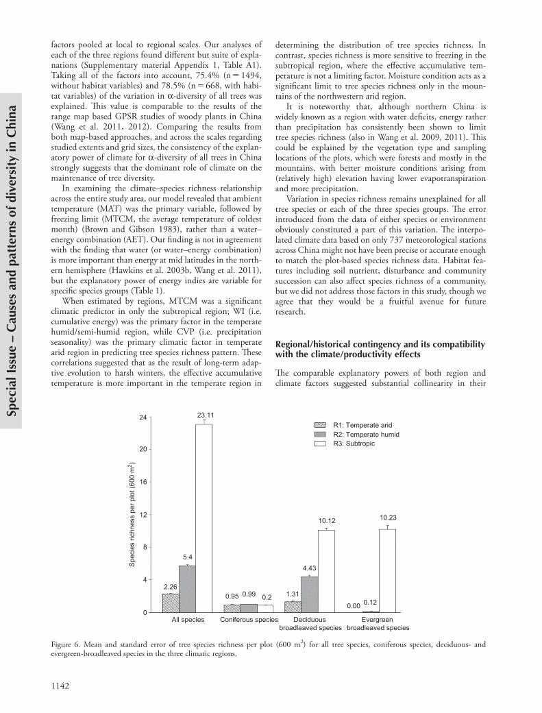
Figure 6. Mean and standard error of tree species richness per plot (600 m2) for all tree species, coniferous species, deciduous- and evergreen-broadleaved species in the three climatic regions.

1143


hina

–1

–0.8

–0.6

–0.4

–0.2

0

0.2

0.4

0.6

0.8

0 1000 2000 3000 4000

sn_sregionelevMATAP

Spatial distance (km)

Mor

an’s

I

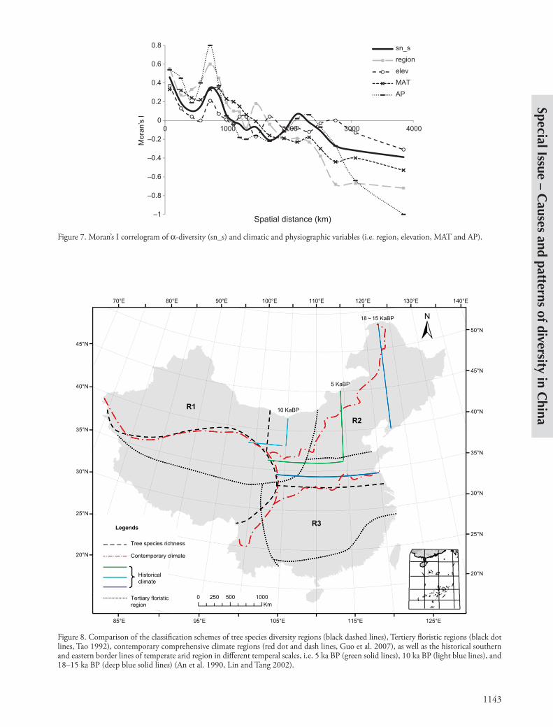
Figure 7. Moran’s I correlogram of a-diversity (sn_s) and climatic and physiographic variables (i.e. region, elevation, MAT and AP).

70°E

85°E

Legends

Tree species richness

Contemporary climate

Tertiary floristicregion

Historicalclimate

95°E

0 250 500 1000Km

105°E 115°E 125°E

80°E 90°E 100°E 110°E 120°E

18 ~ 15 KaBP

5 KaBP

10 KaBPR1

R2

R3

130°E 140°E

50°N

45°N

40°N

35°N

30°N

25°N

20°N

45°N

40°N

35°N

30°N

25°N

20°N

Figure 8. Comparison of the classification schemes of tree species diversity regions (black dashed lines), Tertiery floristic regions (black dot lines, Tao 1992), contemporary comprehensive climate regions (red dot and dash lines, Guo et al. 2007), as well as the historical southern and eastern border lines of temperate arid region in different temperal scales, i.e. 5 ka BP (green solid lines), 10 ka BP (light blue lines), and 18–15 ka BP (deep blue solid lines) (An et al. 1990, Lin and Tang 2002).

1144

Spec

ial I

ssue

– C

ause

s an

d pa

tter

ns o

f div

ersi

ty in

Chi

na

and the correspondence between the extant tree species richness pattern (Fig. 2) and the floristic regions in Neogene suggest temporal autocorrelation in both the change of environment and biodiversity patterns. On the other hand, the significant spatial autocorrelation was also revealed in the Moran’s I curves between species richness, region and climatic variables (Fig. 7). The spatial and temporal auto-correlations existed both within and between the patterns of the species richness and climate might imply the rela-tionship between the climate/productivity hypothesis and regional/historical hypothesis as continuous vs discrete perspectives for GPSR (Supplementary material Appendix 1, Fig. A2). In other words, the contemporary environment (dominated by climate) implicitly included the regional/historical contingency. But on the other hand, the regional/historical contingency, which was basically caused by physiographical barriers and isolation to abiotic and biotic processes, has caused the regional differentiation of both biodiversity and the environment, including regional climate.

Acknowledgements – We are grateful to Anping Chen, Liping Li, Shilong Piao, Xiujuan Qiao and Shuqing Zhao for their help in data collection. We appreciate Bradford Hawkins’ help on English. This study is part of the projects supported by Chinese National Natural Science Foundation (no. 31021001, 31170449, 40638039, 31061160184/C020203).

References

An, Z. et al. 1990. Preliminary study on ancient environmental evolution of Chinese in latest twenty thousand years. – In: Liu, D. and An, Z. (eds), Loess Quaternary geology global changes: vol. II. Science Press, pp. 1–12.

Bini, L. M. et al. 2009. Coefficient shifts in geographical ecology: an empirical evaluation of spatial and non-spatial regression. – Ecography 32: 193–204.

Breiman, L. et al. 1984. Classification and regression trees. – Chapman and Hall.

Brown, J. H. and Gibson, A. C. 1983. Biogeography, 1st ed. – Mosby.

Carrara, R. and Vázquez, D. P. 2010. The species–energy theory: a role for energy variability. – Ecography 33: 942–948.

Currie, D. J. 1991. Energy and large-scale patterns of animal- and plant-species richness. – Am. Nat. 137: 27–49.

Currie, D. J. and Francis, A. P. 2004. Regional versus climatic effect on taxon richness in angiosperms: reply to Qian and Ricklefs. – Am. Nat. 163: 780–785.

Davies, R. G. et al. 2007. Topography, energy and the global distribution of bird species richness. – Proc. R. Soc. B 274: 1189–1197.

Fang, J. 1992. Study on the geographic elements affecting tem-perature distribution in China. – Acta Ecol. Sin. 12: 97–104.

Fang, J. and Lechowicz, M. J. 2006. Climatic limits for the present distribution of beech (Fagus L.) species in the world. – J. Biogeogr. 33: 1804–1819.

Fang, J. et al. 2012. Forest community survey and the structural characteristics of forests in China. – Ecography 35: 1059–1071.

Field, R. et al. 2008. Spatial species-richness gradients across scales: a meta-analysis. – J. Biogeogr. 36: 132–147.

Francis, A. P. and Currie, D. J. 2003. A globally consistent richness–climate relationship for angiosperms. – Am. Nat. 161: 523–536.

effects on species richness pattern (Table 1). With the hierarchical variance partitioning, we attempted to untangle the effects of contemporary climate variables and regional historical effects (Fig. 5). Region as a variable can indepen-dently explain 10.7% of a-diversity for all trees, and 3.1, 9.9 and 5.0% of a-diversity of coniferous, deciduous and evergreen broadleaved species, respectively. These values are considerable with the independent role of the leading single climatic variable in corresponding models. Our results were also comparable to those of Wang et al. (2012) with map-based grid data (50 50 km), which found that the independent contribution of the regional effect to be about 6% for spatial variation in woody plant species rich-ness. Moreover, the regional effect in our analysis was also partially illustrated by the distinction of species group com-positions among the three regions (F 1,297.4, p 0.001) (Fig. 6), i.e. a-diversity of conifers was almost the same for all three regions, evergreen broadleaved trees distributed almost only in the subtropic region, and there were signifi-cant differences of deciduous species richness among the three regions.

The contemporary pattern of biodiversity is a product of historical environment (Hawkins et al. 2003a). Although we proposed the three region scheme based on species richness data, the pattern also received support from geo-logical and fossil evidence, with five floristic regions in China tracing back to late Neogene (23.1–2.5 Ma BP) (Tao 1992), including three regions in our scheme, a Tibet-Himalaya region and a marginal tropical region in southern China. The Quaternary climate changes in China were characterized by glacier/interglacier cycling. In the last glacial maximum period (18–15 ka BP), the north western arid desert and semi-arid grassland extended to 34.5°N in the south and 122.5°E in the east, with 10–12°C lower temperature and 50% less precipitation than the present (An et al. 1990). In the Holocene warm-humid stage (10 ka BP), the arid and semi-arid climate withdrew to 38°N and 105°E. These were the worst and the best stages of climate in China in the last 20 ka BP (Lin and Tang 2002). In last 5 ka BP, the global climate cooled down and aridity intensified again, the southeast boundary of Chinese desert and grassland extend eastward to 114°E, and southward to 36°N (An et al. 1990, Lin and Tang 2002). These spatial dynamics of climate in last 20 ka BP in China not only consistently emphasized a latitudinal tem-perature gradient in the east of China, and a longitudinal moisture gradient in the north of China, but also reflected the regional difference of stability of climate among the three regions, i.e. a stable temperate arid region, a temperate sub-arid to sub-humid region with much more obvious longitudinal (moisture) variability, and a stable humid subtropic region (Fig. 8). The temporal autocorrelation of climate change would leave significant signal to the contem-porary climate, as validated by a study of modern climate regionalization scheme, which was based on the 1970–1999 climatic data from 737 standard meteorological stations across China, and had the same five regions across China (Guo et al. 2007), and coincide with our species richness pattern (Fig. 8).

Therefore, the connection between Quaternary climate processes and contemporary climate pattern across China,

1145


hina

Prentice, I. C. et al. 1992. A global biome model based on plant physiology and dominance, soil properties and climate. – J. Biogeogr. 19: 117–134.

Qian, H. 2008. Effects of historical and contemporary factors on global patterns in avian species richness. – J. Biogeogr. 35: 1362–1373.

Qian, H. and Ricklefs, R. E. 1999. A comparison of the taxonomic richness of vascular plants in China and the United States. – Am. Nat. 154: 160–181.

Qian, H. and Ricklefs, R. E. 2000. Large-scale processes and the Asian bias in species diversity of temperate plants. – Nature 407: 180–182.

Qian, H. and Ricklefs, R. E. 2004. Taxon richness and climate in angiosperms: is there a globally consistent relationship that precludes region effects? – Am. Nat. 163: 773–779.

Rahbek, C. et al. 2007. Predicting continental-scale patterns of bird species richness with spatially explicit models. – Proc. R. Soc. B 274: 165–174.

Rangel, T. F. et al. 2010. SAM: a comprehensive application for spatial analysis in macroecology. – Ecography 33: 46–50.

Ricklefs, R. E. 1987. Community diversity: relative roles of local and regional processes. – Science 235: 167–171.

Ricklefs, R. E. 1999. Global patterns of tree species richness in moist forests: distinguishing ecological influences and historical contingency. – Oikos 86: 369–373.

Ricklefs, R. E. 2004. A comprehensive framework for global patterns in biodiversity. – Ecol. Lett. 7: 1–15.

Ricklefs, R. E. 2008. Disintegration of the ecological community. – Am. Nat. 172: 741–750.

Ricklefs, R. E. and Jenkins, D. G. 2011. Biogeography and ecology: towards the integration of two disciplines. – Phil. Trans. R. Soc. B 366: 2438–2448.

Rohde, K. 1992. Latitudinal gradients in species diversity: the search for the primary cause. – Oikos 65: 514–527.

Rosindell, J. et al. 2011. The unified neutral theory of biodiver-sity and biogeography at age ten. – Trends Ecol. Evol. 26: 340–348.

Svenning, J.-C. and Skov, F. 2005. The relative roles of environ-ment and history as controls of tree species composition and richness in Europe. – J. Biogeogr. 32: 1019–1033.

Svenning, J.-C. and Skov, F. 2007. Ice age legacies in the geographical distribution of tree species richness in Europe. – Global Ecol. Biogeogr. 16: 234–245.

Tao, J. 1992. The territory vegetation, flora and floristic regions in China. – Acta Phytotax. Sin. 30: 25–43 in Chinese with English abstract.

Thornthwaite, C. W. and Hare, F. K. 1955. Climatic classification in forest. – Unasylva 9: 51–59.

Turner, J. R. G. 2004. Explaining the global biodiversity gradient: energy, area, history and natural selection. – Basic Appl. Ecol. 5: 435–448.

Turner, J. R. G. et al. 1987. Does solar energy control organic diversity? Butterflies, moths and the British climate. – Oikos 48: 195–205.

Walsh, C. and Mac Nally, R. 2007. The hier.part package. ver. 1.0-2. Hierarchical partitioning. Documentation for R: a language and environment for statistical computing. – www.rproject.org .

Wang, L. 1996a. Impacts of orientations of slopes and elevation on rainfall in mountainous regions. – Sci. Geogr. Sin. 16: 150–158.

Wang, L. 1996b. The temperature calculation model for the mountainous areas in north China and its application. – J. Nat. Resour. 11: 150–156.

Wang, X. et al. 2009. Relative importance of climate vs local factors in shaping the regional patterns of forest plant rich-ness across northeast China. – Ecography 32: 133–142.

Guo, Z. et al. 2007. Regionalization and integrated assessment of climate resource in China based on GIS. – Resour. Sci. 29: 2–9.

Hawkins, B. A. 2004. Are we making progress toward under-standing the global diversity gradient? – Basic Appl. Ecol. 5: 1–3.

Hawkins, B. A. 2012. Eight (and a half ) deadly sins of spatial analysis. – J. Biogeogr. 39: 1–9.

Hawkins, B. A. et al. 2003a. Productivity and history as predictors of the latitudinal diversity gradient of terrestrial birds. – Ecology 84: 1608–1623.

Hawkins, B. A. et al. 2003b. Energy, water, and broad-scale geographic patterns of species richness. – Ecology 84: 3105–3117.

Holdridge, L. R. 1947. Determination of world plant formations from simple climatic data. – Science 105: 367–368.

Hurlbert, A. H. and White, E. P. 2005. Disparity between range map- and survey-based analyses of species richness: patterns, processes and implications. – Ecol. Lett. 8: 319–327.

Hurlbert, A. H. and Jetz, W. 2007. Species richness, hotspots, and the scale dependence of range maps in ecology and conservation. – Proc. Natl Acad. Sci. USA 104: 13384– 13389.

Jetz, W. and Rahbek, C. 2002. Geographic range size and determinants of avian species richness. – Science 297: 1548–1551.

Kerr, J. T. and Packer, L. 1997. Habitat heterogeneity as a deter-minant of mammal species richness in high-energy regions. – Nature 385: 252–254.

Kumar, S. et al. 2006. Spatial heterogeneity influences native and nonnative plant species richness. – Ecology 87: 3186–3199.

LaSorte, F. A. and Hawkins, B. A. 2007. Range maps and species richness patterns: errors of commission and estimates of uncertainty. – Ecography 30: 649–662.

Latham, R. E. and Ricklefs, R. E. 1993. Global patterns of tree species richness in moist forests: energy-diversity theory does not account for variation in species richness. – Oikos 67: 325–333.

Leprieur, F. et al. 2008. Fish invasion in the world’s river systems: when natural processes are blurred by human activities. – PLoS Biol. 6: 404–410.

Lessard, J.-P. et al. 2011. Strong influence of regional species pools on continent-wide structuring of local communities. – Proc. R. Soc. B 279: 266–274.

Lin, N. and Tang, J. 2002. Geological environment and causes for desertification in arid and semiarid regions in China. – Environ. Geol. 41: 806–815.

Mac Nally, R. 2002. Multiple regression and inference in ecology and conservation biology: further comments on iden-tifying important predictor variables. – Biodivers. Conserv. 11: 1397–1401.

Nogués-Bravo, D. et al. 2008. Scale effects and human impact on the elevational species richness gradients. – Nature 453: 216–220.

O’Brien, E. M. et al. 2000. Climatic gradients in woody plant (tree and shrub) diversity: water–energy dynamics, residual variation and topography. – Oikos 89: 588–599.

Olea, P. P. et al. 2010. Estimating and modeling bias of the hierarchical partitioning public-domain software: implications in environmental management and conservation. – PLoS One 5: e11698.

Palmer, M. W. 1994. Variation in species richness: toward a unification of hypotheses. – Folio Geobot. Phytotax. 29: 511–530.

Pimm, S. L. and Brown, J. H. 2004. Domains of diversity. – Science 304: 831–833.

1146

Spec

ial I

ssue

– C

ause

s an

d pa

tter

ns o

f div

ersi

ty in

Chi

na

Whittaker, R. et al. 2001. Scale and species richness: toward a general hierarchical theory of species diversity. – J. Biogeogr. 28: 453–470.

Willig, M. R. et al. 2003. Latitudinal gradients of biodiversity: pattern, process, scale and synthesis. – Annu. Rev. Ecol. Evol. Syst. 34: 273–309.

Wright, D. H. 1983. Species–energy theory: an extension of species–area theory. – Oikos 41: 496–506.

Wu, Z. Y. et al. (eds) 2002–2012. Flora of China. – www. efloras.org/flora_page.aspx?flora_id 2.

Wang, Z. et al. 2011. Patterns, determinants and models of woody plant diversity in China. – Proc. R. Soc. B 278: 2122–2132.

Wang, Z. et al. 2012. Relative role of contemporary environment versus history in shaping diversity patterns of China’s woody plants. – Ecography 35: 1124–1133.

White, E. P. and Hurlbert, A. H. 2010. The combined influence of the local environment and regional enrichment on bird species richness. – Am. Nat. 175: E35–E43.

Supplementary material (Appendix ECOG-00049 at www.oikosoffice.lu.se/appendix ). Appendix 1.

Geographical patterns of community-based tree species...

Documents

Transcript of Geographical patterns of community-based tree species...