1

Geographic Portfolio Allocations, Property Selection, and Performance Attribution in Public and Private Real Estate Markets

by

David C. Ling*, Andy Naranjo*, and Benjamin Scheick+

*Department of Finance, Insurance, and Real Estate Warrington College of Business Administration

University of Florida Gainesville, Florida 32611

Email: ling@ufl.edu; andy.naranjo@warrington.ufl.edu Phone: (352) 273-0313; (352) 392-3781

+Department of Finance

Villanova School of Business Villanova University

Villanova, Pennsylvania, 19085 Email: benjamin.scheick@villanova.edu

Phone: (610) 519-7994

Current Draft: January 2016

Abstract:

This paper examines the effects of geographic portfolio concentration on the return performance of U.S. public REITs versus private commercial real estate over the 1996-2013 time period. We document significant cross-sectional and temporal differences in the geographic concentration of property holdings across public and private real estate markets. Adjusting private market returns for differences in geographic concentrations with public markets, we find that core private market performance falls. This performance drop arises primarily from lower geographically adjusted retail performance. In contrast, geographically adjusted industrial and office property performance rises slightly while apartment performance remains relatively unchanged. Using return performance attribution analysis, we find that the geographic allocation effect constitutes only a small portion of the total return difference between public and private market returns, whereas individual property selection within geographic locations explains, in part, the documented outperformance of public versus private real estate market returns. This result also suggests that the decision to allocate to a geographic location is relatively less important than the manager’s ability to select and manage properties within that location.

JEL classification: G11, G12, G23, L25, R33 Keywords: real estate investment trusts, private commercial real estate, return performance, portfolio allocation and selection We thank Greg MacKinnon, Brad Case, Mike Grupe, Calvin Schnure, Kevin Scherer, Tim Riddiough, Jeff Fisher, Joe Pagliari, and Jim Shilling, as well as participants in the 2015 NAREIT/AREUEA Real Estate Research Conference in New York, the Summer 2015 NCREIF Conference, and the 2015 Homer Hoyt meetings in Florida for helpful comments and suggestions. We thank NAREIT for providing partial financial support for this project.

2

1. Introduction

The ability to transform illiquid assets into more liquid assets through the issuance of investment

securities has been a major financial innovation. This innovation has played a fundamental role in the

allocation of capital and resources as well as market efficiency. However, this transformation raises an

important question: do investors achieve similar risk and return outcomes by investing directly in the

illiquid assets versus indirectly through a more liquid security? Real estate investments provide an

important, on point, case. Both direct private and stock exchange-listed REITs can provide investors

with exposure to the same underlying local property markets. In each case, returns to investors are

primarily a function of the income streams generated by the property portfolio and fluctuations in the

appreciation component of property values. However, in evaluating the relative ex post investment

performance of listed REIT and private commercial real estate (CRE) markets, it is critical to control for

differences in the underlying characteristics of the two markets and their benchmark return indices. For

example, return performance in the private commercial real estate market is often proxied by the

National Council of Real Estate Investment Fiduciaries (NCREIF) Property Index (NPI). However,

differences in property mix and the treatment of leverage and management fees, compared to that of

listed REIT market indices, may lead to incorrect performance comparisons and inferences between

private and public markets.

Several prior studies find that investments in direct private real estate, as proxied for by the NPI,

produce lower average returns than comparable investments in publicly-traded real estate investment

trusts (REITs), even after adjusting for differences in financial leverage, property mix, and management

fees (Pagliari, Scherer, and Monopoli, 2005; Riddiough et al., 2005). More recently, Ling and Naranjo

(2015) find that passive portfolios of unlevered core REITs (unconditionally) outperformed their private

market benchmark by 49 basis points (annualized) from 1994 to 2012. Although Ling and Naranjo (2015)

and the aforementioned studies carefully control for (firm-level) leverage, property type, and

management fees in their comparisons of public and private market returns, they do not adjust for

differences in the geographic composition of property portfolios across markets.

The need to adjust for Metropolitan Statistical Area (MSA) geography at the portfolio level is not

well-motivated from a financial economics perspective.1 In theory, idiosyncratic MSA risk is diversifiable.

1

In June of 2003, the U. S. Office of Management and Budget (OBM-https://www.whitehouse.gov/omb/inforeg_statpolicy#ms) adopted new standards for Metropolitan Areas and established Core Based Statistical Areas (CBSA). These standards replace and supersede the previous standards used to define Metropolitan Statistical Areas (MSA). CBSAs are divided into two categories: Metropolitan Statistical Areas and Micropolitan Statistical Areas. A MSA is a CBSA associated with at least one urbanized area with a population of at least 50,000, based on the 2000 Census. As of June 6, 2003, the OMB has defined a total of 362 Metropolitan Statistical Areas that incorporate 1,090 counties, containing approximately 83% of the US population.

3

Thus, we would not expect to observe large variations in ex ante risk premiums across MSAs among

otherwise similar properties. However, significant variation in ex post MSA returns suggests that

relative performance differences may be driven by the timing and selection of geographic market entry

and exit. As a result, an important unanswered question in the literature remains; to what extent are

the measured performance differences between equity REITs and the private direct market attributable

to the magnitude and timing of MSA-level property sector allocations?

Recent research suggests that certain institutional features of public REIT markets may inhibit

a manager’s ability to vary geographic allocations in accordance with real estate cycles. For example,

Muhlhofer (2013) focuses on the so-called “dealer rule” as a trading constraint that prevents certain

REITs from consistently generating appreciation returns from portfolio disposition decisions. Muhlhofer

(2015) extends this analysis to examine how these disposition constraints may hinder a REITs ability to

time the property market. Furthermore, Hochberg and Muhlhofer (2014) find little evidence that REIT

managers have the ability to time property type and geographic market entry and exit. This line of

research has two important implications. First, in the presence of trading constraints, geographic

allocation differences across markets have the potential to be persistent. Second, if REIT managers are,

in fact, limited in their ability to allocate to geographies in a timely manner, it is important to understand

the proportion of their relative performance attributable to geographic allocation versus asset selection

within a particular location.2

This paper contributes to the existing literature by addressing the extent to which public and

private market performance differences are attributed to differences in the geographic distribution of

REIT-owned properties relative to NCREIF properties. To the extent that portfolio managers actively

shift geographic and property type allocations to time real estate cycles and also vary in their ability to

select value-adding properties within property types and geographic regions, relative performance can

differ significantly between these two markets. We also contribute to the broader geographical allocation

effects literature by documenting the influence of geographic allocation effects on both the measurement

and evaluation of relative return performance across public and private commercial real estate markets.

In our analysis, we employ a two-stage approach to examine the role that the geographic

compositions of REIT and private market property portfolios have on relative return performance. We

first examine the extent to which geographic allocations within property type vary across publicly-listed

and private CRE markets. We then evaluate the impact that controlling for geography has on relative

2 In a similar line of research that focuses on REIT security selection rather than property selection, Cici et al. (2011) find that fund managers generate significant positive alpha with their selection ability but that geographic concentration strategies do not explain the selection outperformance.

4

return performance. An important difference in our approach from that of many prior studies (e.g., Ling

and Naranjo, 2015) is that we adjust the geographic composition of the benchmark NPI index to mirror

that of our public market REIT portfolio.3 With these careful refinements, we then compare

geographically reweighted NPI returns to unlevered REIT returns and thereby assess the relative

performance of “geographically identical” public and private market portfolios.

We attribute residual performance differences after geographically reweighting NPI returns to

property (asset) selection and management (operational, transaction, and corporate) within MSAs.

Operational management is important because properties are typically held for long periods of time and

generate much of their total return from periodic cash flows as opposed to price appreciation (Geltner,

2003).4 The management of the transaction can also add or destroy value. It is difficult in illiquid and

segmented private real estate markets to determine true market value and therefore reservation prices.

Moreover, the transaction process is often complex and its outcome influenced by the negotiation skills

of the buyer and seller. At the corporate level, REIT managers can also affect stock prices by their

management of dividend policy and capital raising decisions.

In addition to operational, transaction, and entity-level management, we recognize that residual

performance differences could also be partially attributable to time-varying volatility and liquidity risk

premiums. For example, it is well documented that equity REIT returns respond to movements in the

general stock market, especially in the short-run. This stock market-induced volatility can cause REIT

returns to be more volatile than the underlying value of REIT assets (Clayton and MacKinnon, 2003).

This additional layer of volatility, if priced by the capital markets, may generate higher risk premiums

and therefore higher ex post returns. Furthermore, publicly-traded REITs are more liquid investments

than direct ownership of commercial real estate. This liquidity is valuable and therefore reduces the ex

ante risk premium required by REIT investors. The volatility and liquidity risk premium effects are at

least partially offsetting and their time-varying magnitudes are difficult to estimate. Thus, they may too

account for a portion of observed ex post pubic versus private market performance differentials.5

3

Riddiough et al. (2005) note that differences in index composition related to geographic asset allocations may be an important source of return differences across markets. However, the authors cite a lack of reliable data on asset holding locations during their sample period as a primary reason for this omission from their analysis. 4

Operational management functions include marketing and leasing as well as the management of operating expenses and capital expenditures. 5

In our comparison of relative performance, we also recognize that return differences may still be related to other index composition issues such as the proportion of development properties in each portfolio or differences in property subtype allocations. As of the beginning of 2013, development properties with available estimated cost data constituted approximately one percent of properties in the REIT property portfolio, thereby mitigating concern that they are a major driver of relative performance differences. To address whether differences in property subtype allocations influence our main findings, we later perform an additional robustness check within the Retail sector and find similar results.

5

To measure the MSA risk exposures of publicly-traded equity REITs, we first obtain time-varying

property level location data from SNL’s Real Estate Database. From this information, we compute the

percentage allocations of equity REIT portfolios to each MSA at the beginning of each year. This allows

us to compare the MSA concentrations of publicly-traded REITs, by core property type (i.e., apartments,

industrial, office, and retail) and for all core properties, to the MSA concentrations of the properties in

the NCREIF database over the 1996-2013 sample period. We then calculate the extent to which adjusting

for these differences in MSA exposure affects the NPI returns reported by NCREIF. This is accomplished

by obtaining quarterly MSA-level NCREIF NPI returns for the four core property types and then

reweighting these MSA-level returns to create returns for each core property type using the same time-

varying MSA weights observed in the REIT data.

We document significant differences in geographic allocations of property portfolios between

listed REIT and private markets. These differences vary significantly over time and across property type

classifications. We further establish the extent to which accounting for time-series and cross-sectional

differences in the geographic concentrations of the properties held by core equity REITs and NCREIF

investors affects performance comparisons across markets. Adjusting private markets for differences in

geographic concentrations with public markets, we find that core private market performance falls.

Focusing on property types, we find the biggest return difference in the retail sector. The benchmark

average return for retail NPI properties is 10.6 basis points lower than the corresponding unadjusted

quarterly NPI return over our sample period; thus, its use in place of the unadjusted (published) NPI

retail return increases the measured outperformance of REIT investors. In contrast, the reweighted

mean returns for industrial and office properties are 1.9 and 4.4 basis points, respectively, greater than

the corresponding unadjusted quarterly NPI return. Thus, using reweighted returns slightly decreases

the average performance of industrial and office REITs relative to the performance of NCREIF investors

in these property types over the 1996-2013 sample. NPI returns for apartment properties over the full

sample period remain unchanged after reweighting by geography, though significant differences emerge

over shorter investment horizons.

In addition to providing an improved methodology for comparing public and private market

portfolio returns, our geographically reweighted indices also enable us to use attribution analysis to

isolate the extent to which measured performance differences between listed equity REITs and the NPI

benchmark are attributable to MSA-level property sector allocations. While conditional return-based

investment performance regression analysis can estimate risk-adjusted alphas and identify style tilts, it

is limited in its ability to decompose investment returns into potential manager value-added dimensions

6

such as sector/MSA allocation and asset selection. However, this decomposition is important in providing

a clearer understanding of investment return sources.6

We find that the MSA allocation effect constitutes a small portion of the total return difference

across public and private commercial real estate markets. This indicates that decisions to allocate to

particular MSAs are relatively less important than other determinates of return differences, including

the manager’s ability to select and manage properties within that MSA. This is consistent with Capozza

and Seguin’s (1999) positive selection effect hypothesis. This result holds across a variety of sample

periods and within property type and subtype classifications.7 However, the sign and magnitude of the

pure allocation effect varies significantly over the sample period and property type being examined.

Regarding the fundamental question of whether investors achieve similar risk and return

outcomes by investing in listed equity REITs versus investing directly in the private market, our results

suggest that listed equity REITs are real estate. This is especially true as the length of the investment

horizon increases and short-term return differences driven by stock market-induced volatility and time-

varying liquidity in the listed market dissipate.

The remainder of the paper proceeds as follows. The next section provides an initial comparison

of public and private market performance over the 1996-2013 sample period without adjustments for

differences in geographic allocations across markets. Section 3 describes our MSA level data and

discusses our methodology for adjusting benchmark returns for differences in MSA concentrations.

Section 4 presents a formal attribution analysis that examines the extent to which differences in ex post

returns between public and private markets are attributable to differences in MSA allocations. Section

5 provides the results of a number of robustness checks addressing issues of sample period dependence

and property subtype analyses. We provide concluding remarks in the final section. Details of the de-

6

The investment performance evaluation literature is voluminous, dating back to the 1960’s with conditional return-based Jensen’s alpha and Sharpe ratio performance measures as well as their many multifactor model extensions (e.g., Jensen (1968), Sharpe (1964), Fama and French (1992, 1993), and Carhart (1994), among many others). However, an important concern with these returns-based model approaches is that they are joint tests of the underlying benchmark model being used and the statistical and economic significance of the measured performance. More recently, research attention has turned towards developing measures of portfolio performance that allow weights to play a more central role in the formation of the benchmark against which return performance is measured. These weights are often based on portfolio holdings and the characteristics of those holdings (e.g., Grinblatt and Titman (1989), Brinson, Hood, and Beebower (1986), Brinson, Singer, and Beebower (1991), Grinblatt and Titman (1993), Grinblatt, Titman, and Wermers (1995), Zheng (1999), Daniel, Grinblatt, Titman, and Wermers (1997), Kacperczyk, Sialm and Zheng (2005, 2008), Griffin and Xu (2009), among others). Our approach is grounded in this more recent performance attribution characteristic weighting approach, where our weights are the MSA-level REIT and private market property locations. In contrast to traditional characteristic-based approaches whose focus is on decomposing the sources of fund return performance attributable to characteristic selectivity, characteristic timing, and average style exposure (or industry), our focus is on attributing the relative performance of REITs versus private market real estate returns for each property type into asset MSA allocation and property selection. 7 Pavlov and Wachter (2011) suggest that the selection ability of REIT managers relative to their private market counterparts should be less prominent during periods of economic growth but valued significantly during periods of economic stagnation. However, our results suggest that the selection effect is equally important in boom, bust, and recovery periods.

7

levering process used to create the unlevered return series for core REITs, a breakdown of our sample

construction by geographic concentration measure, and a simplified example of how our methodology

can provide REIT managers with an additional tool for analyzing firm-level performance are provided

in Appendices A, B, and C, respectively.

2. Public vs. Private Market Returns: 1996-2013

It is well known that significant differences in financial leverage and property type mix

complicates performance comparisons across public and private markets (Pagliari et al., 2005, Riddiough

et al., 2005; Ling and Naranjo, 2015). To render total returns on equity REIT portfolios comparable to

unlevered private market returns, it is necessary to adjust the composition and risk characteristics of

publicly-traded REIT portfolios to match as closely as possible the composition and characteristics of

their benchmark private market portfolios. Following the methodology of Ling and Naranjo (2015), we

(1) remove the effects of financial leverage from firm-level REIT returns, (2) exclude from the final

analysis those equity REITs that do not invest in core property types, and (3) construct unlevered total

return series for each of the four core property classifications.8 No explicit adjustments are made to

reflect the exposure of publicly-traded REITs to stock market-induced volatility or the liquidity

advantage that publicly-traded REITs enjoy relative to private market investments.

Our initial list of publicly-traded U.S. equity REITs is obtained from the CRSP-Ziman database.

We collect the following data for each REIT at the beginning of each quarter: REIT identification number,

property type and sub-property type focus, and equity market capitalization. We also obtain levered

monthly total returns for each REIT in our sample from CRSP-Ziman, which we then compound to

produce the levered total return on equity for each REIT in a particular quarter.

We obtain the balance sheet and income statement information necessary to unlever quarterly

returns at the firm level by merging our initial REIT sample with data collected from the quarterly

CRSP/Compustat database. A detailed explanation of the delevering process and property type

adjustments used to create the unlevered return series for core REITs is available in Appendix A.

Our primary source of return data in the private CRE market is the National Council of Real

Estate Investment Fiduciaries (NCREIF). Established in 1982, NCREIF is a not-for-profit industry

8 A REIT is included in our retail index if it is classified by CRSP-Ziman as having a property type focus of 9 (retail) and a sub-property type focus of 5 (freestanding), 14 (outlet), 15 (regional), 17 (shopping center), or 18 (strip center). Our industrial index includes REITs classified by CRSP-Ziman as having a property type focus of 4 (industrial/office) and a sub-property type focus of 8 (industrial). Our quarterly office sample includes REITs with a property type focus of 4 (industrial/office) and a sub-property type focus of 13 (office). Finally, a REIT is included in our apartment index in a given quarter if it is assigned by CRSP-Ziman a property type focus of 8 (residential) and a sub-property type focus of 2 (apartments).

8

association that collects, processes, validates, and disseminates information on the risk/return

characteristics of commercial real estate assets owned by institutional (primarily pension and

endowment fund) investors (see www.ncreif.org). NCREIF’s flagship index, the NCREIF Property Index

(NPI), tracks property-level quarterly returns on a large pool of properties acquired in the private market

for investment purposes only. The property composition of the NPI changes quarterly as data

contributing NCREIF members buy and sell properties. However, all historical property-level data

remain in the database and index.

Any analysis of the relative return performance between public and private real estate returns

must address the well-known smoothing and stale appraisal problems associated with the NCREIF NPI.9

Our solution is to compare public and private market returns over time horizons of at least six years.

Such an approach largely mitigates the problems associated with smoothing and stale appraisals.10

Since firm-level REIT returns are net of all firm-level management fees, we must also adjust

downward our quarterly NPI returns because they are reported gross of management fees. According to

industry sources, investment management fees as a proportion of assets under management range

between 50 and 120 basis points per year in the direct private market (see, for example, Riddiough et

al., 2005; Ling and Naranjo, 2015). We conservatively estimate total advisor/management fees to be 80

basis points per year (20 bps per quarter) in our formal analysis.

Table 1 reports quarterly geometric means of our unlevered equity REIT returns (Panel A),

unlevered raw NPI returns (Panel B), and the difference in geometric means across property types (Panel

C) for the following periods: 1996-2001, 2002-2007, 2008-2013, and 1996-2013. “Raw” NPI returns are

those reported by NCREIF. The aggregate, core properties return in each panel is constructed by value-

weighting the four core property type returns in each quarter using the market value property type

weights of the NPI. We find that value-weighted portfolios of unlevered core REITs (unconditionally)

outperform their private market benchmark by three basis points per quarter (12 basis points annually)

from 1996-2013. However, comparisons of public and private market return performance are sensitive

9 Unless a constituent property happens to sell during the quarter, the reported quarterly capital gain on an individual property within the NCREIF NPI is based on the change in the property’s appraised value. Appraisal-based indices are thought to suffer from two major problems. First, estimated price changes lag changes in “true” (but unobservable) market values; this smoothing of past returns understates return volatility. Second, formal appraisals of constituent properties in the NCREIF Index by third party appraisers are usually conducted annually; the property’s asset manager is responsible for updating the appraisal internally in the intervening quarters. This leads to what is commonly called the “stale” appraisal problem. 10 In addition to the NPI, NCREIF also produces a suite of Transaction Based Indices (TBIs). An advantage of the TBI indices is that the capital gain component of the TBI in each quarter is based only on the constituent properties in the NCREIF database that were sold that quarter. The TBI indices are available from NCREIF at the national level back to 1994Q1 for multifamily, office, industrial, and retail properties. However, these core TBI indices are not available at the MSA level, which precludes their use in this research.

9

to the time period selected for the analysis and the property type being examined. Focusing on the

comparison of our core return series, the relative outperformance of equity REITs is concentrated in the

most recent recovery period (2008-2013) as REITs outperformed their private market benchmark by 60

(240) basis points quarterly (annually). However, during the 1996-2001 and 2002-2007 time periods, core

REITs underperformed their private market benchmark by 11 and 41 basis points quarterly,

respectively. Apartment, office, and retail REITs all outperformed the raw NPI series in the recent

recovery period (2008-2013). However, in earlier sub-periods, only retail REITs (from 1996-2001) and

industrial REITs (from 2002-2007) outperformed their private market benchmarks. These return

comparisons further underscore the importance of controlling for the mix of property types and carefully

considering the appropriate investment horizon when comparing the relative performance of REIT and

private market return series.11

3. Differences in MSA Allocations

The return differences reported in Panel C of Table 1 control for differences in leverage, property

type, and management fees. However, these return differences do not account for time-series and cross-

sectional differences in the geographic concentrations of the properties held by core equity REITs and

the data contributing members of NCREIF (primarily pension and endowment funds). Thus, from this

comparison we are unable to determine the portion of public-private performance differences

attributable to MSA allocations.

If idiosyncratic MSA risk is diversifiable, we would not expect to observe large variations in ex

ante risk premiums across MSAs among otherwise similar properties. This expectation is borne out in a

variety of survey data. For example, the Real Estate Investment Survey, the results of which are

published quarterly in the Real Estate Report by the Real Estate Research Corporation (RERC),

summarizes information on current investment criteria, such as acquisition cap rates, required rates of

return on equity, and expected rental growth rates.12 In 2014Q1, RERC reported required unlevered

rates of return for nine property types across 48 of the most important MSAs. We focus our example on

the major “gateway” MSAs, most frequently defined as Boston, Chicago, Los Angeles, New York, San

11

Some REITs that primarily invest in one of the four “core” property types, and are therefore included in our sample, nevertheless own assets that would not be considered ‘class A” properties. In contrast, the NCREIF properties used to construct the NPI are largely, if not exclusively, class A properties. To the extent REIT portfolios contain less then class A properties which, on average, are risker, we would expect mean REIT returns to be higher, all else equal. 12 The survey respondents are a sample of CRE investors, lenders, fee appraisers, and managers in the U.S. The survey focuses on “institutional grade” assets that are owned and financed by pension and endowment funds, life insurance companies, private equity funds, investment banks, and real estate investment trusts. A distinct advantage of the RERC data is the ability to abstract required unlevered rates of return by property type and major MSA. For more details, see http://store.rerc.com/collections/real-estate-repor.

10

Francisco, and Washington, D.C. It is important to note that the gateway MSAs are widely thought to

be less risky markets than the majority of MSAs. One reason often cited for the lower perceived risk

profile of these markets is that the ability for developers to add new supply, which could reduce rents

and prices, are severely constrained. In addition, these major markets are thought to be more liquid,

which would in theory drive down risk premiums.

As displayed in panel A of Table 2, the mean required rate of return for apartment properties in

the first quarter of 2014 was 7.28 percent; the standard deviation of required returns across these six

MSAs was just 0.13 percent. For CBD office properties (panel B of Table 2), the mean required return

was 7.97 percent and the standard deviation was 0.27 percent. Thus, despite differences in the expected

prospects for these gateway MSAs, there is remarkably little variation in required returns in early 2104.

This strongly suggests investors are unable to detect large variations in systematic risk across these

major MSAs.

However, an examination of ex post MSA returns suggests something much different. For the six

gateway MSAs, we obtained unlevered realized returns for the most recent six-year period (2008-2013)

as well as realized returns over the full sample. The mean realized return for apartment properties in

the gateway markets was 4.69 percent during 2008-2013 with a standard deviation of 3.26 percent. The

mean realized return over the 18-year study period was 7.68 percent during with a standard deviation

of 3.22 percent. Thus, despite significant variation in realized returns across these six markets prior to

the 2014Q1 survey, market participants were not able to detect ex ante differences in systematic risk for

these gateway markets. We observe similar relations using data for CBD office properties in panel B of

Table 2. This apparent disconnect between expected returns and realized MSA returns suggests that

relative performance differences may still be driven by the timing and selection of geographic market

entry and exit.

To examine the importance of time-varying geographic concentrations, we collect the following

data from SNL’s Real Estate Database on an annual basis for each property held by an equity REIT

during the period 1996 to 2013: the property owner (institution name), property type, geographic location

(MSA), acquisition date, sold date, book value, initial cost, and historic cost. Our analysis begins in 1996

(end of 1995) because this is the first period for which SNL provides historic cost and book value

information at the property level. Although the property composition of the aggregate REIT portfolio

changes as properties are bought and sold, all historical property-level data remain in the SNL database.

Over our 1996-2013 sample, we have 517,131 property-year observations in our REIT dataset. At

the beginning of 1996, equity REITs held 15,752 properties with a reported book value of over $34 billion.

The corresponding property counts and book values for core equity REITs are 9,420 and $25 billion,

11

respectively. By the beginning of 2013, equity REITs owned 32,707 properties with a reported book value

of over $419 billion. Core REITs held 15,510 properties with a reported book value of $242 billion. After

excluding non-core REITs, 291,894 property-year observations remain in the sample.

To construct our time-varying measures of geographic allocations, we first sort equity REITs by

their CRSP-Ziman property type and property subtype classifications. We then sort each core REIT’s

properties into MSA categories that mirror those tracked by the NCREIF NPI within a particular year.

We compute the percentage of the REIT portfolio held in an MSA by REITs of property type f at the

beginning of year T as follows:

, , ∑ , ,

,

∑ ∑ , ,,

, 1

where , , is the “adjusted cost” of property i in Metropolitan Statistical Area m at the

beginning of year T. ADJCOST is defined by SNL as the maximum of (1) the reported book value, (2) the

initial cost of the property, and (3) the historic cost of the property including capital expenditures and

tax depreciation.13 Of our 291,894 property-year observations for core REITs, 197,387 (68 percent)

contain adjusted cost information.14 The total number of properties of type f in a particular MSA at the

beginning of year T is denoted as Nm,T. The total number of NCREIF MSA classifications as of the

beginning of year T is denoted as NT.

As a robustness check, we create additional time-varying geographic concentration measures for

each of the four property types. First, we replace the adjusted cost of each property by its book value. 15

Of our 291,894 property-year observations, 197,387 (65 percent) contain book value information.16 It is

important to note that the use of adjusted cost or book value in place of true market values may

understate the (value-weighted) percentage of the REIT portfolio that is invested in MSAs that have

recently experienced a relatively high rate of price appreciation. Conversely, the use of adjusted cost or

book value may overstate the percentage of the REIT portfolio in MSAs that have experienced relatively

large price declines.

13 SNL’s initial cost variable (SNL Key Field: 221778) is defined as the historic cost currently reported on the financial statements, which may be different than the cost reported at time of purchase. SNL’s historic cost variable (SNL Key Field: 221782) is defined as the book value of the property before depreciation. 14

For more information on the extent to which the adjusted cost field is populated by year by property type, see Appendix B. 15 SNL’s net book value variable (SNL Key Field: 221784) is defined as the historical cost of the property and improvements, net of accumulated depreciation. 16 See Appendix B for more detailed information.

12

We also consider two additional geographic allocation approaches: a simple property count

measure and the square footage of properties held within an MSA. However, each of these approaches

has its own limitations relative to using book value or adjusted cost. While property count allows us to

maximize our sample size without any loss of observations, it does not capture relative value differences

of properties within and between MSAs. Thus, to the extent that valuations differ in the geographical

cross-section of property portfolios, the use of property count weights can yield significantly different

inferences about relative performance.

Similar to Hochberg and Muhlhofer (2014), we also use square footage of properties held by equity

REITs as an additional geographic allocation weight. However, this measure suffers from the same

limitation as our simple property count variable because valuations per square foot vary significantly

across MSAs. In addition, square footage data is only available for approximately 60 percent of core

property-year observations in the SNL database over our sample period.17 Although our aggregate

results are qualitatively similar using these alternate measures of geographic exposure, we use adjusted

cost and book value as our primary measures of geographic concentrations to mitigate the

aforementioned concerns.

To compare the geographic exposure of the NCREIF portfolio with that of our sample of equity

REITs, we calculate geographic concentrations for each of the four core property NCREIF NPI portfolios

as follows:

, , ∑ , ,

,

∑ ∑ , ,,

, 2

where , , is the market (appraised) value of property i in Metropolitan Statistical Area m at the

beginning of year T.18 The total number of properties of type f in a particular MSA at the beginning of

year T is denoted as Nm,T. The total number of MSA classifications as of the beginning of year T is again

denoted as NT.

The NCREIF NPI at the beginning of 1996 was composed of 2,379 core properties with an

estimated market value of $50 billion. NCREIF does not report a quarterly return for property type f in

MSA m unless there are at least four properties available for the return calculation. This is done to

protect the identity of the individual properties and owners. We classify the MSA location of properties

17

See Appendix B for more details on sample construction descriptive statistics. 18

The lagged and smoothed nature of the NPI will cause the calculated percentage of the NCREIF portfolio invested in MSAs experiencing rapid price appreciation to be understated. Conversely, the use of appraisal values will overstate the percentage of the NPI portfolio in MSAs experiencing rapid price declines.

13

held outside of the NCREIF MSAs with reported returns as “Other.” By the beginning of 1996, the NPI

contained four or more apartment, industrial, office, or retail properties in 58 MSAs, with its greatest

concentration in Washington, D.C. (7.1 percent). In comparison, equity REITs held 6.7 percent of their

core portfolio (based on adjusted cost) in the D.C. area. By the beginning of 2013, the NPI index contained

6,968 core properties with an estimated market value of $366 billion. The NPI database contained four

or more of one of the core properties in 106 MSAs, with its greatest concentration in New York (10.4

percent). Equity REITs held 13.1 percent of their core assets in New York in 2013.

3.1. Allocations to Gateway MSAs

Much has been written by industry professionals about the desirability of investing in major

gateway MSAs. These MSAs are thought to have significant investment advantages over the remaining

300-plus MSAs, including increased liquidity, due to the size and depth of these markets. In addition,

constraints on the production of new supply in these MSAs put upward pressure on rental rates.

Therefore, the degree to which public and private market investors allocate investment capital to these

markets, as well as the timing of these investments, may be an important determinant of their portfolio’s

performance. This important question has not been addressed in the academic literature.

In Figure 1, we present the concentrations of equity REIT and NCREIF core properties located

in gateway MSAs. On average, NCREIF investors held approximately 34 percent of their portfolio in

gateway MSAs over our 1996 to 2013 sample period; equity REITs held approximately 31 percent of their

core assets in these six metropolitan areas. However, we observe larger differences in allocations over

time and by property type. For example, REITs held a slightly larger portion of their core portfolio in

gateway MSAs from 2001 to 2006. However, as the recent credit crisis unfolded, NCREIF investors held

a significantly higher proportion of their portfolio in these six cities. In fact, in 2008 NCREIF investors

increased their concentrations in gateway MSAs to constitute nearly 40 percent of their core portfolio.

In Panel A of Figure 2, we present allocations to gateway MSAs for apartment properties. Panels

B-D of Figure 2 display geographic concentrations in these six markets for industrial, office, and retail

properties, respectively. There are several key takeaways from these comparisons. First, within a

particular year there are often significant differences between the proportion of properties held by

NCREIF data contributing members and those held by equity REITs in gateway markets. For example,

in 2003 equity REITs held approximately 50 percent of their industrial assets in gateway cities (Figure

2, Panel B). During the same year, NCREIF investors held just 21 percent of their industrial property

portfolio in these six major markets.

14

Second, the relative weighting of REIT property portfolios toward gateway cities is persistent.

During most of our sample period, equity REITs hold larger portions of their apartment, industrial, and

office properties in gateway cities. Since 2003, however, NCREIF investors have been significantly more

exposed to gateway retail than equity REITs.

Third, we observe significant variation in the time-series distribution of these portfolio

concentrations. For example, from 2000-2013 equity REITs increased the concentration of their

apartment portfolios in gateway markets from approximately 10 percent to nearly 50 percent. This

represents a massive reallocation of REIT apartment portfolios to gateway markets. In contrast, REIT

allocations to gateway cities within the industrial property type have been more cyclical. For example,

from 1996-2003 equity REITs increased their holdings of industrial properties in gateway cities by

approximately 20 percent. However, from 2004-2008 equity REITs shifted their industrial portfolio away

from gateway cities, decreasing their holdings from 50 percent of their portfolio to approximately 33

percent.

In both the apartment and office property type, changes in portfolio holdings in gateway markets

appear to be positively correlated across investor types for much of our sample period. From 2000-2013,

both equity REITs and NCREIF investors increased their exposure to gateway apartment properties by

40 and 20 percent, respectively. During this same period, both equity REITs and NCREIF investors also

significantly increased their office holdings in gateway cities by 20 percent and 10 percent, respectively.

For industrial properties, on the other hand, we observe a significant negative correlation

between changes in gateway allocations by equity REITs and NCREIF investors. While equity REITs

shifted their industrial portfolio away from gateway cities from 2004-2008, NCREIF investors increased

the proportion of industrial properties owned in these markets from 19 percent to 28 percent of their

portfolio. In the retail sector, however, there is less correlation between changes in concentration across

investor groups. Since 2005, equity REITs have maintained a fairly consistent allocation to gateway

markets in their retail portfolios, ranging from 18 percent to 20 percent. In contrast, NCREIF investors

have reduced their allocations to gateway retail from 30 percent to 20 percent during the same period.

In comparing public and private market gateway concentrations across property types, it is evident that

differences exist within a particular year and across time.

As we narrow our focus to portfolio concentrations in specific gateway cities, the points observed

previously at the aggregate level become more evident. In Figure 3, we present the concentrations of

equity REIT and NCREIF apartment properties located in Chicago.19 As observed in the aggregate data,

19

The corresponding figures for the remaining five gateway MSAs are available from the authors upon request.

15

there are significant differences between the proportion of properties held by NCREIF data contributing

members and those held by listed equity REITs, persistence in REIT weighting toward gateway cities,

significant variation in the time-series distribution of these portfolio concentrations, and notable

differences across property types when comparing listed REIT and private market geographic

concentrations within a gateway MSA. For example, in 2013 NCREIF investors held approximately 7.0

percent of their apartment assets in Chicago. During the same year, equity REITs held approximately

1.0 percent of their apartment assets in Chicago. Looking more broadly over the full sample period,

NCREIF investors consistently held a significantly larger portion of their apartment portfolio in Chicago

than equity REITs. From 2006 to 2013, NCREIF investors substantially increased the concentration of

their apartment portfolios in Chicago, while equity REITs were decreasing their exposure to apartment

properties in Chicago during this period. These are strikingly different “bets” on the attractiveness of

the Chicago apartment market. In sharp contrast, since at least 2006 public and private market

investors have allocated similar proportions of their capital to Chicago industrial and office properties.

Finally, in recent years NCREIF investors have been significantly more exposed to Chicago retail

properties than retail REITs.

There are also noticeable differences in how NCREIF investors and equity REITs allocate their

portfolios to specific gateway markets within property types. For example, apartment REITs hold a

relatively larger proportion of their apartment assets in Los Angeles, Washington, D.C., Boston, and San

Francisco; in contrast, NCREIF investors tend to dedicate greater concentrations of their apartment

portfolio to Chicago than equity REITs. The two groups of investors hold similar proportions of their

apartment portfolio in New York. Overall, it is clear that the MSA composition of NCREIF and REIT

apartment, industrial, office, and retail portfolios often varies significantly across gateway markets at a

particular point in time; moreover, these relative allocations can also vary significantly over time. It is

therefore important to understand the extent to which these differences in MSA allocations affect the

return performance of public and private market investors, both in the short- and long-run.

3.2. Have Gateway MSAs Outperformed?

To determine how these differences in gateway allocations may impact portfolio returns it is

important to first establish that there are in fact significant performance differences between gateway

and non-gateway markets. To conduct this analysis, we begin with quarterly NCREIF NPI returns

disaggregated by property type and MSA. We then create a value-weighted gateway return series for

each property type, as well as an aggregate core property series, in which the weights are the market

(appraised) values of properties held by NCREIF within each of the six gateway cities as of the beginning

16

of the year. Similarly, we construct value-weighted non-gateway return series in which the weights are

the market (appraisal) values of properties held by NCREIF in each of the remaining non-gateway

cities.20

Table 3 reports quarterly geometric means of our gateway NPI returns (Panel A), non-gateway

NPI returns (Panel B), and the difference in means between gateway and non-gateway returns (Panel

C) for the following periods: 1996-2001, 2002-2007, 2008-2013, and 1996-2013. We report mean returns

for each of the four core property types, as well as an aggregate value-weighted core property type series.

Over the full sample, gateway markets outperform non-gateway markets for all property type

classifications, including the aggregate core series. In fact, the only indication of underperformance in

gateway markets appears in the recovery period for apartment and industrial properties. In the

aggregate, gateway markets outperformed non-gateway markets by 26 (106) basis points quarterly

(annually) over the 1996-2013 sample period. The most significant difference in performance between

gateway and non-gateway markets at the property type level is in the office sector, which outperformed

non-gateway office investments by 44 basis points quarterly. During the period of rapid expansion in

commercial real estate markets (2002-2007), this return difference was even larger as gateway office

markets outperformed non-gateway markets by 96 basis points quarterly.

To further establish differences in performance across MSAs, we also calculate quarterly

geometric means of NPI returns for each of the six gateway cities by core property type. Although not

separately tabulated, we find significant variation in returns within each property type across the six

gateway markets. In addition, relative performance varies significantly across our three sub-sample

periods.

3.3. Adjusting Private Market Returns for Differences in MSA Concentrations

The observed differences in the MSA concentrations of core property investments and

performance differences across gateway MSAs highlights the importance of controlling for MSA

exposure, particularly if both public and private investment managers have at least some discretion over

the MSAs in which they are able to invest. We therefore reweight NPI MSA-level returns using the time-

varying MSA weights of the corresponding REIT portfolio, as detailed in equation (1). In particular, for

each core property type f, the total MSA-reweighted NPI return in quarter t is defined as:

, , , , , , , . . . , , , 3

20 Though not separately tabulated, we obtain similar results when using equally-weighted portfolios.

17

where , is the NPI total return for property type f in Metropolitan Statistical Area n in quarter t

and , is the (adjusted cost) weight of the REIT property portfolio concentrated in Metropolitan

Statistical Area n and property type f as of the beginning of year t. This weighting and aggregation

process is repeated each quarter to produce a time series of reweighted NPI returns for each of the four

core property types from 1996Q1 to 2013Q4. Note that we hold our MSA weights, , , constant across

quarters within a calendar year. However, the reweighted return ( , ) varies quarterly because

the MSA-level NPI return ( , ) varies quarterly.

We also construct an adjusted aggregate core property NPI total return series using NCREIF

market value property type weights. We first calculate quarterly property type weights using the market

value of all properties held by the NPI for each of the four core property type classifications. More

specifically, the core portfolio weight assigned to property type f in quarter t is:

, ,

∑ ,, 4

where f = 1…4 for multifamily (apartment), office, industrial and retail properties, respectively, and

MVf,t is the total market value of properties held by the NCREIF portfolio within property type f as of

the beginning of quarter t. Thus, the total return in quarter t on our core-properties reweighted NPI

index is defined as:

, , , 5

where , is the total return on our reweighted NPI index for property type f in quarter t as

detailed in equation (3). This aggregation of property type NPI returns is repeated each quarter to

produce a time series of aggregate core reweighted NPI returns.

Table 4 provides summary statistics for the quarterly differences between our raw NPI and

reweighted NPI return series, by core property type and by reweighting methodology. The reweighted

mean NPI apartment return using adjusted cost weights (Panel A) is equal to the unadjusted NPI

apartment return over the full sample. The median return, standard deviation, and serial correlation of

the reweighted NPI apartment returns are also very similar in magnitude to the corresponding summary

statistics for the unadjusted NPI apartment returns.

The reweighted mean returns for industrial and office properties, using adjusted cost weights,

are 1.9 and 4.4 basis points, respectively, greater than the corresponding unadjusted quarterly NPI

18

return. Thus, using reweighted returns slightly increases the average performance of industrial and

office NCREIF investors relative to the performance of REIT investors in these property types over the

1996-2013 sample. In contrast, the reweighted mean return for retail NPI properties is 10.6 basis points

lower than the corresponding unadjusted NPI return; thus, its use in place of the unadjusted NPI retail

return decreases the measured relative performance of NCREIF investors. The reweighted quarterly

mean return for core NPI properties is 1.4 basis points lower than the corresponding unadjusted NPI

return; thus, core private market performance falls slightly after adjusting private market returns for

differences in geographic concentrations with public markets. Overall, the small magnitude of the

differences in NPI returns that results from reweighting are striking.

The differences in geographically reweighted NPI returns and unadjusted NPI returns are very

similar when MSA weights are based on the time-varying book value of REIT properties (Table 4, Panel

B). In untabulated results using REIT weights based on property count and square footage, we continue

to find that the reweighted mean return for core NPI properties is less than the corresponding

unadjusted NPI return. These additional findings further suggest that our core property adjusted return

results are robust to alternate measures of geographic concentrations.21

The geographic reweighting of apartment, industrial, and office properties using REIT allocations

does not produce notable differences in mean or median private market returns over the full sample.

However, these sample means and medians mask significant differences over time as shown by the large

minimum and maximum differences in Table 4. To better display this time-series variation in return

differences, we plot quarterly differences between reweighted and unadjusted NPI returns for apartment

properties in Panel A of Figure 4. The dashed red line plots differences using MSA weights based on the

adjusted cost of the underlying REIT properties. The solid (blue) line captures quarterly differences in

returns assuming MSA weights are based on the book value of the underlying REIT properties. A point

on any curve greater than zero percent indicates the reweighted NPI return for apartments in that

quarter is greater than the unadjusted NPI return; that is, the unadjusted NPI return understates the

performance of the NPI for the purpose of comparing private market performance to returns on equity

REITs.

Although the mean return difference for apartment properties is clearly centered around zero,

there are significant quarterly differences over the 1996 to 2013 sample period. For example, in the

21 At the property type level, the results show more variability because the use of square footage significantly reduces the number of property-year observations within property types and simple property count weights do not capture relative value differences between MSAs.

19

second quarter of 2005, the reweighted NPI return (using adjusted cost) is less than the unadjusted

return by 0.94 percentage points (94 basis points), or 376 basis points annually. In contrast, the

reweighted NPI return is greater than the unadjusted NPI return in the first quarter of 2007 by 77 basis

points, or 308 basis points annually. These are large and economically meaningful differences that could

significantly distort short-run comparisons between public and private real estate markets.

In Panels B-D of Figure 4, we plot quarterly differences in reweighted and unadjusted NPI total

returns for industrial, office and retail properties, respectively. Similar to apartment properties,

reweighting MSA-level NPI returns produces large changes in many quarters. For example, in the fourth

quarter of 2008, reweighted NPI office returns are less than unadjusted office returns (adjusted cost

value geographic concentrations) by 137 basis points (548 basis points annually). Similarly large

differences in quarterly returns are observable in the industrial and retail property returns. In addition,

the return differences can remain positive, or negative, for sustained periods of time. The serial

correlations of the return differences (last column in Table 3), especially for industrial and office

properties, also indicate statistically significant persistence in return differences. Given that many

investment management contracts have durations of three-to-five years, these persistent differences

could significantly affect the measured performance of a manager.

4. Attribution Analysis

A primary objective of the current research is to better understand the extent to which the return

differences in public and private CRE markets reported in Table 1 are attributable to differences in MSA

allocations. It is generally impossible to define unique, break-downs of total returns that correspond to

clear investment management functions. Nevertheless, useful insights can be obtained from

performance attribution.

Assume that both REIT and NCREIF managers do not have discretion over the core property

type in which they invest. Assume also that the effects of leverage have been removed from the

underlying REIT returns in the REIT portfolio. Then, for property type f in quarter t, the difference in

REIT and NCREIF NPI total returns, , - , , is equal to:

, , = allocation + selection + interaction, (6)

where allocation is the portion of the return differential due to MSA allocations. Selection is defined as

the portion due to property/asset picking and operational management; although, as discussed above,

the performance difference not explained by MSA allocations could be partially attributable to the

combined effects of time-varying stock market-induced volatility and liquidity risk premiums on REIT

20

returns, in addition to the relative property selection and management skills of REIT managers. From

here forward we refer to the sum of these decisions/effects as the “selection” component of the return

differential. Finally, interaction is the portion of the return differential that results from the synergy

between allocation and selection decisions. The interaction effect is positive when a REIT manager over-

weights MSAs in which she has positive property selection and management ability and underweights

MSAs in which she does not.

Using the total unlevered return earned by NCREIF managers on property type f in quarter t as

the benchmark, we can attribute the differential performance of REIT managers to allocation, ,

, , and selection, , , . The pure effect of REIT managers’ asset allocation, relative to the

benchmark return of NCREIF NPI mangers, is quantified as the sum across all MSAs of the difference

between REIT allocation and NCREIF allocation to an MSA, multiplied by the NCREIF NPI return in

that MSA. More formally, the return differential for property type f in quarter t attributable purely to

differences in MSA allocations is

, , = ⋯ , (7)

where is the NPI return in MSA n in quarter t, is the percentage of the REIT portfolio invested

in MSA n in quarter t, and is the percentage of the NCREIF portfolio invested in MSA n in quarter

t.

The pure effect of REIT managers’ asset selection in quarter t, relative to the benchmark NCREIF

NPI return, is quantified as the sum across all MSAs of the difference between the REIT portfolio’s

return and the NPI return in an MSA, weighted by the allocation of the NCREIF NPI portfolio in that

MSA. More formally, the return differential attributable to differences in property/asset selection is

, , = ⋯ , (8)

where is the return on the REIT portfolio in MSA n.

As detailed in equation (6), the sum of the pure allocation and selection effects do not equal the

total differential between REIT and NCREIF NPI returns. The remaining differential is due to the

combined effect of REIT managers’ allocation and selection performances interacting together.

Unfortunately, there is no meaningful way to disentangle this interaction effect and allocate it to either

one of the two pure effects. Typically, if the allocation of capital across MSAs is the primary decision

facing REIT and NCREIF managers, the interaction effect is added to the selection effect to keep the

allocation effect pure. This would be appropriate, in this application, if REIT mangers generally pursued

21

a top-down investment strategy (MSA selection then property selection). In contrast, if REIT managers

generally follow a bottom-up investment strategy—finding the best properties without a primary concern

for MSA allocations—it would be appropriate to add the interaction effect to the allocation effect to keep

the selection effect pure. However, our primary objective is to quantify the importance of MSA allocation

decisions in explaining differences in public and private market return performance. Moreover, data on

REIT returns by property type at the MSA level ( in equation (8) above) are not available. We are

therefore unable to calculate a pure selection effect (using the private market return series as our

benchmark) and thus must lump together the pure selection and interaction effects.22

Performing attribution analysis for one quarter, as depicted in equation (7), is relatively straight-

forward if the MSA-level NPI returns ( ), as well as NPI and REIT MSA weights ( and ),are

known. However, NPI and REIT portfolio allocations change over time and these changes must be

accounted for when explaining relative performance over the duration of a typical asset management

contract, or longer.

To facilitate a multi-year attribution analysis, we start with equation (7). Using the distributive

property and regrouping terms, equation (7) can be rewritten as

, , … ) -

… . 9

Note that the top term in parentheses is the return on the reweighted NPI for property type f in quarter

t (i. e. , , fromequation 3 , using REIT allocations for the reweighting. The bottom term in

parentheses is simply the “raw” NPI return for property type f in quarter t. Thus, by subtracting the raw

NPI return for a particular property type from the re-weighted NPI, we are left with the pure allocation

effect in quarter t using NPI as the benchmark.

For a T quarter analysis period, equation (9) can be rewritten as follows to produce the geometric

average return differences over T quarters:

, , ∏ 1 , -1) – ( ∏ 1 , - 1) . (10)

22 An argument can be made for using REIT returns and MSA weights as the benchmark in equations (7) and (8), respectively. This allows us to calculate a pure selection effect; however, the interaction effect must then be included with the allocation effect due to the lack of available MSA-level REIT return data. In untabulated results, the use of REIT MSA weights and returns in place of NPI weights and returns does not alter the relative magnitudes of the allocation and selection effects reported in Table 5.

22

Table 5 displays results from our attribution analysis using adjusted cost weights and NPI returns as

the benchmark for each of the four core property types, as well as the aggregate core property type series.

We report in each panel the quarterly difference in geometric means between our unlevered REIT

returns and the raw NPI returns, the geometric mean of the pure allocation effect, and the geometric

mean of the selection plus interaction effects.

In each of the core property types and for all reported return horizons, the pure allocation effect

constitutes a small portion of the total return difference relative to the selection plus interaction effects.

This indicates that the decision to allocate to a particular MSA is relatively less important than the

manager’s ability to select and mange properties within that MSA. However, the sign and magnitude of

the allocation effect varies significantly over time and across property types. For example, retail REITs

outperformed their NPI benchmark by 16.9 basis points quarterly over the full sample. The pure

allocation decisions of REIT managers actually resulted in a 10.5 basis point quarterly

underperformance relative to the private market benchmark. However, the asset selection (plus

interaction) of REIT managers produced an outperformance of 27.3 basis points. In this case, the

allocation of REIT properties across MSAs reduced the positive outperformance of equity REIT’s

generated by superior asset selection and management. In each of the three sub-periods, the MSA

allocation of the REIT retail portfolio also reduced the relative outperformance of retail REITs. In all

sub-periods, the allocation effect is smaller in magnitude that the selection and interaction effect.

In contrast to retail REITs, industrial REITs (panel B) underperformed their NPI benchmark

over the full sample and in two of the three sub-periods. However, the pure allocation effect is negative

only in the 1996-2001 subperiod. Thus, the underperformance of industrial REITs is driven by selection

(and interaction) effects, except during the 2002-2007 subperiod. Nevertheless, the pure allocation effects

in the industrial sector are small in magnitude relative to the selection and interaction effects. For core

portfolios (panel E), the magnitudes of the allocation effects are also small relative to the

selection/interaction effect. Overall, the variation in allocation and selection effects both across time and

across property types is noteworthy. However, the relatively small role that MSA allocations have on

relative performance is striking.

To ensure that our results are not being driven by our choice of geographic concentration measure,

we report results of our attribution analysis using book value in place of adjusted cost weights in Table

6. These results are very similar to those reported in Table 5. This is not surprising given that differences

in reweighted NPI returns produced by the two weighting methodologies are minimal (see Figure 4).

Though untabulated, using property count and square footage weights for our core portfolio analysis, we

continue to find that the magnitude of the allocation effect is small relative to the selection effect. These

23

additional findings further suggest that our core property results are not sensitive to alternate measures

of geographic concentrations.

4.1. Economic Significance

To more formally address the economic significance of the allocation decision we examine the

extent to which the variability in equity REIT returns across time is explained by MSA allocation

decisions. We follow a framework similar to Ibbotson and Kaplan (2000) and report R-squared estimates

from a portfolio regression approach. To first understand the proportion of REIT return variability

explained by its private market benchmark, we regress quarterly unlevered REIT returns on unadjusted

NPI returns. These results are reported in panel A of Table 7. Over the full sample period, raw NPI

returns explain 11.7 percent, 10.6 percent, 4.4 percent, and 6.1 percent of the variation in unlevered

REIT returns for apartment, industrial, office, and retail property types, respectively. Using the

aggregate core series, NPI returns explain 7.8 percent of the variation in unlevered core REIT returns

over the full sample.

The previous regression setup does not allow us to isolate the proportion of return variability

explained by MSA allocation decisions. However, by holding geographic allocations constant between our

two return series, we are better able to isolate the relative importance of REIT geographic allocation

strategy. We regress quarterly unlevered REIT returns against reweighted NPI returns. These results

are reported in panel B of Table 7. If MSA allocations matter, using NPI returns that have the same

MSA weightings as the equity REIT portfolio should improve the explanatory power of the regressions,

despite the smoothing and lagging problems associated with the use of NPI returns in quarterly

regressions. For some property types and time periods, the R-squared improves slightly, while in several

cases the explanatory power of the REIT total return model decreases when using reweighted NPI

returns as the explanatory variable. However, in no case is the difference in R-squareds statistically

significant. The inability of reweighted NPI returns to improve our ability to explain unlevered REIT

returns is consistent with our finding that MSA allocation policies account for a relatively small

proportion of the difference in REIT and NPI returns. Taken together, our results also suggest that

using unadjusted NPI returns tends to overstate the proportion of equity REIT return variation that is

explained by its private market benchmark.

5. Further Robustness Checks: Sample Period Dependence and Property Subtype Analysis

Since geometric means simulate a buy-and-hold strategy, inferences drawn from their use may

be dependent on the assumed investment holding period. The results reported in Tables 5 and 6 assume

24

non-overlapping six-year investment horizons as well as an eighteen-year holding period. In Table 8, we

report results based on six non-overlapping three-year holding periods. With the exception of one window

for industrial properties (2008-2010), we again find that MSA allocation strategies account for a

relatively small portion of the difference in REIT and NPI returns. In fact, this result is generally

stronger with the shorter three-year windows.

To further examine the sensitivity of our results to holding period assumptions, we performed the

analysis using rolling six-year windows starting in the first quarter of 1996. We then averaged

(arithmetically) across these overlapping six-year windows. These results are reported by property type

in panel A of Table 9. The mean quarterly return differential between unlevered REIT returns and raw

NPI is 4.8 basis points for retail properties. The mean MSA allocation effect is -13.3 basis points; that is,

retail REIT managers underperformed the private market retail benchmark with respect to MSA

allocations. However, the asset selection (plus interaction) of retail REIT managers produced a mean

outperformance of 18.0 basis points, somewhat larger in absolute magnitude than the negative allocation

effect. For industrial properties, the average allocation effect is positive, indicating REIT managers

outperformed the data contributing members of NCREIF in selecting and timing MSA allocations.

However, the positive allocation effect of 8.4 basis points was nearly offset, on average, by inferior

selection and management. For apartment, office, and core REITs, the mean allocation effect is small in

absolute magnitude relative to the selection and interaction effect. Thus, our primary result does not

appear to be driven purely by the chosen six-year windows reported earlier in Tables 5 and 6.

To ensure our results are not being driven by a particular sample year, we also performed the

analysis for the 1996-2013 period 18 times, each time dropping a different year from the sample. We

then averaged (arithmetically) across these 18 samples.23 These results are reported by property type in

panel B of Table 9. For all property types, including core REITs, the mean allocation effect is small in

absolute magnitude relative to the selection and interaction effect.

If the selection plus interaction component of our original analysis is also capturing required

allocations to property subtypes rather than pure property selection within a particular MSA, we would

expect the selection plus interaction effect to be relatively less important at the property subtype level.

To address whether differences in property subtype allocations reduce the relative importance of the

selection plus interaction effect, we conduct an additional attribution analysis within the retail property

type classification. In particular, we focus on the shopping center subtype.24 We follow the methodology

23 We thank Andrey Pavlov for this suggestion. 24 Since the NCREIF and CRSP-Ziman property subtype classifications are not a one-to-one match, we group together REITs classified as Shopping Center (property subtype 17) and Strip Center (property subtype 18) REITs as “shopping centers.”

25

described previously to construct an unlevered REIT return series and a geographically reweighted NPI

return series for shopping centers.

Table 10 reports results from our shopping center attribution analysis using NPI returns as the

benchmark. In all but one sub-period (2002-2007) we observe similar results to those reported for the

retail property type in Table 5. The selection effect remains a significant portion of the return difference

between private and public market portfolios. Due to data limitations, we are unable to conduct this

analysis for other property subtypes within the retail or other core property type classifications. Thus,

to the extent that property subtypes can be evaluated, our primary findings are robust.

The discussion to this point has centered on controlling for differences in geographic

concentrations between public and private market investors in an attempt to provide a better benchmark

for return comparisons as well as insights on the relative importance of allocation and selection in return

performance at the portfolio level. However, our methodology can also be applied on a firm level basis.

For example, REIT managers and investors can utilize our reweighting procedure to generate a private

benchmark return series that is “geographically identical” to their particular portfolio. They also can

utilize the attribution framework to better understand how allocation and selection decisions impact

firm return performance relative to a chosen benchmark. An example of a firm level application is

provided in Appendix C.

6. Conclusion

While direct private and public REIT investments can provide investors with exposure to the

same underlying local property markets, they often exhibit substantially different risk-return

characteristics. Thus, when evaluating relative investment performance the construction of a similar-

risk benchmark index is of utmost importance. This study identifies the importance and respective

influences of geographic allocation and selection effects on both the measurement and evaluation of

relative return performance across public and private commercial real estate markets. By adjusting

returns for differences in financial leverage, property type focus, management fees, and geographic

concentrations we are able to more accurately assess the relative performance of “geographically

identical” public and private market portfolios. Furthermore, through formal attribution analysis, we

are able to disentangle whether the relative return performance is attributable to differences in MSA

allocations or individual property selection and management within MSAs.

Properties classified by NCREIF as Community, Neighborhood, or Power Centers are used to construct our NCREIF shopping center returns.

26

To the extent that portfolio managers actively shift geographic allocations to time real estate

cycles and vary in their ability to select value-adding properties within property types and geographic

regions, relative performance can differ significantly across investment markets. In comparing the MSA

concentrations of publicly-traded REITs, by core property type, to the MSA concentrations of the

properties in the NCREIF database, we document material differences in geographic allocations of

property portfolios between public and private market investors. Since these differences vary

substantially over time and across property type classifications, we find that accounting for time-series

and cross-sectional differences in the geographic concentrations of the properties held by core equity

REITs and NCREIF investors has an economically meaningful impact on performance comparisons

across markets.

Controlling for the geographic composition of property portfolios in these two markets, we

continue to find that public market real estate returns exceed comparable private market returns.

Through our attribution analysis, we also find that MSA allocations explain a relatively small portion of

the total return difference relative to selection effects. However, the direction and magnitude of this

effect can vary across investment periods and property types. Overall, this result indicates that the

decision to allocate to a particular MSA is relatively less important than the manager’s ability to select

properties within that MSA. Taken together, our results suggest that additional follow-on research

examining geographic allocation and selection effects is important to understanding return performance

and effective investment strategies in both public and private commercial real estate markets. In this

regard, our research reveals an important open question on what factors contribute to explaining the

superior REIT selection effects that we document.

27

Appendix A: Calculating Unlevered REIT Returns

To create our unlevered REIT return series, we follow the methodology outlined in Ling and

Naranjo (2015). The first step in delevering REIT returns at the firm level is to calculate the firm’s

unlevered return on assets (weighted average cost of capital) in each quarter. We estimate the unlevered

return on total assets for REIT i in quarter t, , , as:

, , , , , , , , A1

where , is the levered total return on equity, , is the total return earned by the firm’s long-term and

short-term debt holders in quarter t, and , is the return earned by preferred shareholders. The time-

varying quarterly weights corresponding to equity, debt, and preferred shares in the firm’s capital

structure are denoted as , , , , and , , respectively.

The returns on debt obligations and preferred shares, respectively, are calculated as:

, ,

,, A2

, ,

, , A3

where , is total interest paid to debt holders in quarter t, , is total preferred dividends, ,

is the total book value of short- and long-term debt, and , is the estimated liquidation value of

outstanding preferred shares for REITi at the end of quarter t-1. , is constructed by chain-linking

monthly returns obtained from CRSP-Ziman.

The capital structure weights for each REIT in each quarter are based on the claims of equity, debt,

and preferred shares outstanding at the end of quarter t -1, relative to total assets outstanding, or

, ,

,, A4

, ,

,, A5

28

, ,

,, A6

where , is the market capitalization of the firm’s common shares at the end of quarter t-1 and

TAi,t-1 is the total asset value for REIT i at the end of quarter t-1. Total asset value for REIT i at the end

of quarter t, , , is set equal to

, , , , , A7

An index of unlevered returns on total assets for equity REITs in quarter t, , is constructed

by summing over the weighted unlevered returns earned by each constituent REIT; that is,

, , , 8

where , is REIT i’’s unlevered (total) return on assets [equation (A1)] and

, ,

∑ ,

, 9

When constructing an index of returns on office REITs, for example, Nt equals the number of office REITs

in the sample. Unlevered quarterly returns are compounded to obtain an index of cumulative returns for

our four core property type indices, as well as our aggregate core property type series.

29

Appendix B: Sample Construction

Although our aggregate results are qualitatively similar using alternate measures of geographic exposure,

we focus our main analysis on our measure of adjusted cost. One reason is that it mitigates the loss of

observations that results from using book value or square footage measures. The table provided in this

appendix (Appendix B Table 1) provides the yearly distribution of property observations in the SNL Real

Estate Database for the four core property types across our four concentration measures. In three out of the

four core property types, a significant loss of observations occurs when using square footage in place of either

adjusted cost or book value, with the office property type being the exception. We also identify that this issue

becomes increasingly prominent in the post-2000 sample period. On average, from 2000-2013, the use of

adjusted cost in place of square footage allows for a 10 percent increase in observations. This potential

selection issue reaches an extreme in 2013, during which the use of adjusted cost in place of square footage

allows for a 20 percent increase in overall sample size.

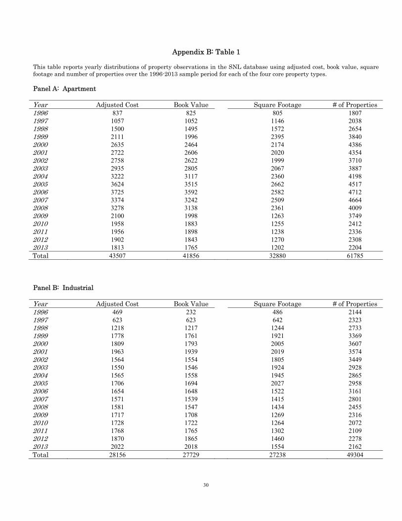
30

Appendix B: Table 1 This table reports yearly distributions of property observations in the SNL database using adjusted cost, book value, square footage and number of properties over the 1996-2013 sample period for each of the four core property types. Panel A: Apartment Year Adjusted Cost Book Value Square Footage # of Properties 1996 837 825 805 1807 1997 1057 1052 1146 2038 1998 1500 1495 1572 2654 1999 2111 1996 2395 3840 2000 2635 2464 2174 4386 2001 2722 2606 2020 4354 2002 2758 2622 1999 3710 2003 2935 2805 2067 3887 2004 3222 3117 2360 4198 2005 3624 3515 2662 4517 2006 3725 3592 2582 4712 2007 3374 3242 2509 4664 2008 3278 3138 2361 4009 2009 2100 1998 1263 3749 2010 1958 1883 1255 2412 2011 1956 1898 1238 2336 2012 1902 1843 1270 2308 2013 1813 1765 1202 2204 Total 43507 41856 32880 61785 Panel B: Industrial Year Adjusted Cost Book Value Square Footage # of Properties 1996 469 232 486 2144 1997 623 623 642 2323 1998 1218 1217 1244 2733 1999 1778 1761 1921 3369 2000 1809 1793 2005 3607 2001 1963 1939 2019 3574 2002 1564 1554 1805 3449 2003 1550 1546 1924 2928 2004 1565 1558 1945 2865 2005 1706 1694 2027 2958 2006 1654 1648 1522 3161 2007 1571 1539 1415 2801 2008 1581 1547 1434 2455 2009 1717 1708 1269 2316 2010 1728 1722 1264 2072 2011 1768 1765 1302 2109 2012 1870 1865 1460 2278 2013 2022 2018 1554 2162 Total 28156 27729 27238 49304

31

Panel C: Office Year Adjusted Cost Book Value Square Footage # of Properties 1996 398 394 401 1460 1997 687 686 772 1731 1998 1423 1408 1460 2504 1999 2096 2085 2118 3122 2000 2201 2180 2223 3227 2001 2139 2115 2270 3122 2002 2318 2275 2443 3199 2003 2302 2253 2419 3098 2004 2290 2242 2409 3039 2005 2213 2166 2341 3034 2006 2270 2201 2377 3197 2007 1890 1549 2056 3107 2008 1567 1495 1635 2600 2009 1603 1531 1658 1967 2010 1631 1537 1695 1896 2011 1660 1567 1716 1912 2012 1662 1564 1711 1930 2013 1565 1512 1642 1960 Total 31915 30760 33346 46105 Panel D: Retail Year Adjusted Cost Book Value Square Footage # of Properties 1996 1308 1282 1525 4009 1997 2392 2297 2554 4438 1998 3000 2917 3135 5024 1999 4004 3913 3790 5897 2000 4567 4502 4404 6400 2001 4467 4371 4384 6721 2002 4601 4507 4639 6743 2003 4743 4649 4809 6841 2004 5209 5075 5056 7249 2005 5739 5015 5446 7736 2006 7329 7038 5792 9669 2007 5828 5536 5633 10229 2008 6098 5856 5577 10738 2009 6550 6315 5524 8407 2010 6494 6278 5368 8270 2011 6802 6598 5284 8435 2012 7142 6961 5167 8710 2013 7536 7373 4976 9184 Total 93809 90483 83063 134700

32

Panel E: Core Properties Year Adjusted Cost Book Value Square Footage # of Properties 1996 3012 2733 3217 9420 1997 4759 4658 5114 10530 1998 7141 7037 7411 12915 1999 9989 9755 10224 16228 2000 11212 10939 10806 17620 2001 11291 11031 10693 17771 2002 11241 10958 10886 17101 2003 11530 11253 11219 16754 2004 12286 11992 11770 17351 2005 13282 12390 12476 18245 2006 14978 14479 12273 20739 2007 12663 11866 11613 20801 2008 12524 12036 11007 19802 2009 11970 11552 9714 16439 2010 11811 11420 9582 14650 2011 12186 11828 9540 14792 2012 12576 12233 9608 15226 2013 12936 12668 9374 15510 Total 197387 190828 176527 291894

33

Appendix C: Sample Apartment REIT We consider the case of a large apartment REIT to implement our framework on a firm level

basis. In particular, we construct unlevered REIT returns for the firm on a quarterly basis following the

methodology of Ling and Naranjo (2015). For our initial comparison to a private market benchmark, we

utilize quarterly raw NPI returns for the apartment property type. We then create a reweighted NPI

return series using NPI MSA-level returns and the time-varying MSA weights of the firm’s property

portfolio, as detailed in equation (3). In particular, the total firm weighted NPI return in quarter t is

defined as:

, , , , , , , . . . , , , C1 where , is the NPI total return in Metropolitan Statistical Area n in quarter t and , is the

(book value) weight of EQR’s property portfolio concentrated in Metropolitan Statistical Area n as of the

beginning of year t.

Panel A of Appendix C Table 1 reports the geometric means for the firm’s unlevered REIT returns,

the raw NPI apartment returns, and the reweighted NPI return series using the firm’s geographic

concentrations as weights. Over each return horizon, the raw NPI series overstates benchmark returns,

although the differences are relatively small in magnitude. For example, over the full sample period

there is a 2.5 (10) basis point quarterly (annually) difference between the raw NPI and the reweighted

NPI that makes use of the firm’s geographic composition. Therefore, the use of the raw NPI series leads

to an overstatement in the relative underperformance of the firm to its private market benchmark.

During the period of generally rising real estate prices (2002-2007), the magnitude of this effect is a bit

larger. The raw NPI overstates the benchmark performance by 5.5 (22) basis points quarterly (annually)

over this horizon. While these differences are relatively small, we expect there to be significant cross-

sectional variation across equity REITs. In particular, we expect this reweighting procedure to matter

most for firms whose geographic concentration differs significantly from that of the benchmark property

type NPI series.

Panel B of Appendix C Table 1 reports results from our firm-level attribution analysis. Consistent

with our earlier results at the portfolio level, we find that the pure allocation effect constitutes a small

portion of the total return difference, relative to the selection plus interaction effects. For example, over

our full sample period the allocation effect constituted 2.5 (10) basis points of the 21 (84) basis point

quarterly (annual) difference between the firm’s unlevered returns and the NPI benchmark apartment

series.

34

Appendix C: Table 1 This table reports quarterly geometric means of the unlevered REIT return for a large apartment REIT, the raw NPI apartment return series, the reweighted NPI index using the firm’s geographic allocations, and firm level attribution analysis using the NCREIF NPI as the benchmark over the following periods: 1996-2001, 2002-2007, 2008-2013, 1996-2013. Returns are reported in percentage form. Panel A: Return Series 1996-

2001 2002- 2007

2008- 2013

1996- 2013

Unlevered REIT Return (firm) 2.177 2.619 1.581 2.125 Raw NPI Returns - Apartment 2.696 2.879 0.840 2.134 Reweighted NPI Returns (using the firm’s weights) 2.696 2.818 0.839 2.113

Panel B: Attribution Analysis 1996-

2001 2002- 2007

2008- 2013

1996- 2013

Unlevered REIT return (firm) minus raw NPI – Apartment -0.519 -0.261 0.741 -0.010 Pure allocation effect -0.001 -0.062 -0.001 -0.021 Selection effect plus interaction -0.518 -0.199 0.742 0.011

35

References

Ambrose, B., S. Ehrlich, W. Hughes and S. Wachter. 2000. REIT Economies of Scale: Fact or Fiction? The Journal of Real Estate Finance and Economics 20: 211–224. Brinson, G.P., L. Randolph Hood, and G. L. Beebower. 1986. Determinants of Portfolio Performance. Financial Analysts Journal 42: 39-48. Brinson, G.P., B. D. Singer, and G. L. Beebower. 1991. Determinants of Portfolio Performance II: An Update. Financial Analysts Journal 47: 40-48. Campbell, R., Petrova, M., Sirmans, C.F.. 2003. Wealth effects of diversification and financial deal structuring: evidence from REIT property portfolio acquisitions. Real Estate Economic 31, 347–366. Capozza, D.R. and P.J. Seguin. 1998. Managerial Style and Firm Value. Real Estate Economics 26: 131–150. Capozza, D.R. and P.J. Seguin. 1999. Focus, Transparency, and Value: The REIT Evidence. Real Estate Economics 27: 587–619. Carhart M. 1997. On Persistence in Mutual Fund Performance. Journal of Finance 52: 57–82. Cici, Gjergji, Jack Corgel, and Scott Gibson. 2011. Can Fund Managers Select Outperforming REITs? Examining Fund Holdings and Trades. Real Estate Economics 39: pgs. 455-486. Clayon, J. and G. MacKinnon. 2003. The Relative Importance of Stock, Bond, and Real Estate Factors in Explaining REIT Returns. Journal of Real Estate Finance and Economics 27(1): 39-60. Daniel, K., M. Grinblatt, S. Titman, and R. Wermers. 1997. Measuring Mutual Fund Performance with Characteristic-Based Benchmarks. Journal of Finance 52(3): 1035-1058. Fama E, French K. 1992. The Cross-Section of Expected Stock Returns. Journal of Finance 47: 427–65. Fama E, French K. 1993. Common Risk Factors in the Returns on Stocks and Bonds. Journal of Financial Economics 33: 3–56. Geltner, D. 2003. IR-Based Property-Level Performance Attribution. Journal of Portfolio Management special issue: 138-151. Griffin J, Xu J. 2009. How Smart are the Smart Guys? A Unique View from Hedge Fund Stock Holdings. Review of Financial Studies 22: 2531-570. Grinblatt M, Titman S. 1989. Mutual Fund Performance: An Analysis of Quarterly Portfolio Holdings. Journal of Business 62: 393-416. Grinblatt M, Titman S. 1993. Performance Measurement without Benchmarks: An Examination of Mutual Fund Returns. Journal of Business 60: 97-112.

36

Grinblatt M, Titman S, Wermers R. 1995. Momentum Strategies, Portfolio Performance and Herding: A study of Mutual Fund Behavior. American Economic Review 85: 1088-1105. Gyourko, J. and E. Nelling. 1996. Systematic Risk and Diversification in the Equity Market. Real Estate Economics 24: 493–515. Hartzell, Jay C., Libo Sun, and Sheridan Titman. 2014. Institutional investors as monitors of corporate diversification decisions: Evidence from real estate investment trusts. Journal of Corporate Finance 25: pgs. 61-72. Hochberg, Yael V. and Tobias Muhlhofer. 2014. Market Timing and Investment Selection: Evidence from Real Estate Investors. Working Paper. Ibbotson R.G. and Kaplan P.D. 2000. Does Asset Allocation Policy Explain 40, 90, or 100 Percent of Performance? Financial Analysts Journal 56(1): 26-33. Jensen M. 1968. The Performance of Mutual Funds in the Period 1945 -1964. Journal of Finance 23: 389-46. Kacperczyk MC, Sialm C, Zheng L. 2005. On the Industry Concentration of Actively Managed Equity Mutual Funds. Journal of Finance 60(4): 1983-2011. Kacperczyk M.C, Sialm C, Zheng L. 2008. Unobserved Actions of Mutual Funds. Review of Financial Studies 21(6): 2379-2416. Ling, David C. and Andy Naranjo. 2015. Returns and Information Transmission Dynamics in Public and Private Real Estate Markets. Real Estate Economics 43(1): 163-208. Muhlhofer, Tobias. 2013. Why do REIT Returns Poorly Reflect Property Returns? Unrealizable Appreciation Gains Due to Trading Constraints as the Solution to the Short-Term Disparity. Real Estate Economics 41(4): 814-857. Muhlhofer, Tobias. 2015. They Would if They Could: Assessing the Bindingness of the Property Holding Constraints for REITs. Real Estate Economics, Forthcoming. Pagliari, Joseph L., Kevin A. Scherer, and Richard T. Monopoli. 2005 Public versus Private Real Estate Equities: A More Refined, Long-Term Comparison. Real Estate Economics 33: pgs. 147- 187. Pavlov, Andrey and Susan M. Wachter. 2011. REITs and Underlying Real Estate Markets: Is There a Link? Working Paper. Riddiough, Timothy J., Mark Moriarty, and P.J. Yeatman. 2005. Privately versus Publicly Held Asset Investment Performance. Real Estate Economics 33: pgs. 121-146. Sharpe W. 1964. Capital Asset Prices: A theory of Market Equilibrium under Conditions of Risk. Journal of Finance 19: 425-442.

37

Zheng L. 1999. Is Money Smart?: A Study of Mutual Fund Investors’ Fund Selection Ability. Journal of Finance 54: 901-933.

38

Figure 1: Gateway City Concentrations of Core Properties – NCREIF vs. REITs This figure plots the geographic concentrations of private (NCREIF) and public (equity REIT) commercial real estate portfolios in gateway cities for all core property types over the 1996-2013 sample period. Gateway cities are defined as Boston, Chicago, Los Angeles, New York, San Francisco, and Washington, D.C. Private market concentrations are calculating using market (appraised) value of each core property held by the NCREIF NPI in gateway cities. Public market concentrations are calculated using reported adjusted cost of each core property held by equity REITs in gateway cities.

39

Figure 2: Gateway City Concentrations by Core Property Type – NCREIF vs. REITs

This figure plots the geographic concentrations of private (NCREIF) and public (equity REIT) commercial real estate portfolios in Gateway cities for each of the four core property types over the 1996-2013 sample period. Gateway cities are defined as Boston, Chicago, Los Angeles, New York, San Francisco, and Washington, D.C. Private market concentrations are calculating using market (appraised) value of each core property held by the NCREIF NPI in gateway cities. Public market concentrations are calculated using reported adjusted cost of each core property held by equity REITs in gateway cities.

Panel A: Apartment Panel B: Industrial

Panel C: Office Panel D: Retail

40

Figure 3: Geographic Concentrations – NCREIF vs. REITs (Chicago)

This figure plots the geographic concentrations of private (NCREIF) and public (equity REIT) commercial real estate portfolios in Chicago for each of the four core property types over the 1996-2013 sample period. Private market concentrations are calculating using market (appraised) value of each core property held by the NCREIF NPI in gateway cities. Public market concentrations are calculated using reported adjusted cost of each core property held by equity REITs in gateway cities.

Panel A: Apartment Panel B: Industrial

Panel C: Office Panel D: Retail

41

Figure 4: Differences in Reweighted NPI Returns and Raw NPI Returns

This figure plots quarterly differences between the reweighted and unadjusted NPI return series for each of the four core property types. The dashed line plots differences using MSA weights based on the adjusted cost of the underlying REIT properties. The solid line captures quarterly differences in returns assuming MSA weights are based on the book value of the underlying REIT properties.

Panel A: Apartment Panel B: Industrial

Panel C: Office Panel D: Retail

42

Table 1: Average Return Comparison: Public and Private Real Estate Markets

This table reports quarterly geometric means of our unlevered equity REIT returns, unlevered raw NPI returns, and the difference between the two series over the following periods: 1996-2001, 2002-2007, 2008-2013, 1996-2013. Returns are reported in percentage form.

Panel A: Unlevered Equity REIT Returns

1996- 2001

2002- 2007

2008- 2013

1996- 2013

Apartment 2.584 2.022 1.728 2.111 Industrial 2.560 3.439 0.133 2.034 Office 2.734 2.346 1.205 2.093 Retail 2.333 3.184 1.692 2.401 Aggregate: Core Properties 2.529 2.659 1.295 2.159

Panel B: Unlevered Raw NPI Returns

1996- 2001

2002- 2007

2008- 2013

1996- 2013

Apartment 2.696 2.879 0.840 2.134 Industrial 2.986 2.926 0.585 2.159 Office 3.095 2.913 0.372 2.119 Retail 1.828 3.742 1.146 2.233 Aggregate: Core Properties 2.637 3.066 0.700 2.129

Panel C: Unlevered REIT Returns minus Unlevered Raw NPI Returns

1996- 2001

2002- 2007

2008- 2013

1996- 2013

Apartment -0.113 -0.857 0.888 -0.024 Industrial -0.426 0.513 -0.452 -0.125 Office -0.361 -0.567 0.833 -0.026 Retail 0.505 -0.558 0.546 0.169 Aggregate: Core Properties -0.108 -0.407 0.595 0.030

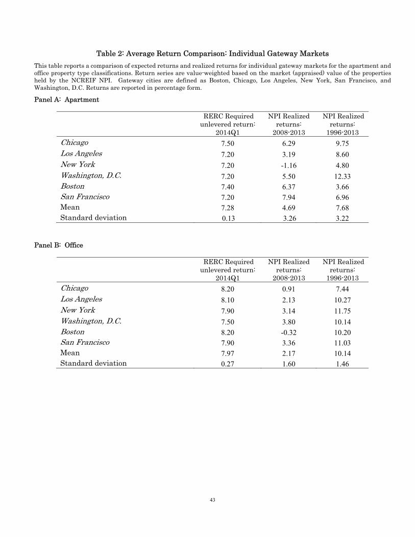
43

Table 2: Average Return Comparison: Individual Gateway Markets

This table reports a comparison of expected returns and realized returns for individual gateway markets for the apartment and office property type classifications. Return series are value-weighted based on the market (appraised) value of the properties held by the NCREIF NPI. Gateway cities are defined as Boston, Chicago, Los Angeles, New York, San Francisco, and Washington, D.C. Returns are reported in percentage form.

Panel A: Apartment

RERC Required unlevered return:

2014Q1

NPI Realized returns:

2008-2013

NPI Realized returns:

1996-2013 Chicago 7.50 6.29 9.75 Los Angeles 7.20 3.19 8.60 New York 7.20 -1.16 4.80 Washington, D.C. 7.20 5.50 12.33 Boston 7.40 6.37 3.66 San Francisco 7.20 7.94 6.96 Mean 7.28 4.69 7.68 Standard deviation 0.13 3.26 3.22

Panel B: Office

RERC Required unlevered return:

2014Q1

NPI Realized returns:

2008-2013

NPI Realized returns:

1996-2013 Chicago 8.20 0.91 7.44 Los Angeles 8.10 2.13 10.27 New York 7.90 3.14 11.75 Washington, D.C. 7.50 3.80 10.14 Boston 8.20 -0.32 10.20 San Francisco 7.90 3.36 11.03 Mean 7.97 2.17 10.14 Standard deviation 0.27 1.60 1.46

44

Table 3: Average NPI Return Comparison: Gateway and Non-Gateway Markets

This table reports quarterly geometric means of unlevered raw NPI returns for gateway and non-gateway markets, and the difference between the two series for each of the four core property types, and all core properties, over the following periods: 1996-2001, 2002-2007, 2008-2013, 1996-2013. Return series are value-weighted based on the market (appraised) value of the properties held by the NCREIF NPI. Gateway cities are defined as Boston, Chicago, Los Angeles, New York, San Francisco, and Washington, D.C. Returns are reported in percentage form.

Panel A: Gateway NPI Returns

1996- 2001

2002- 2007

2008- 2013

1996- 2013

Apartment 3.507 3.376 0.612 2.490 Industrial 3.345 3.437 0.761 2.507 Office 3.388 3.618 0.673 2.551 Retail 2.239 4.308 1.457 2.661 Aggregate: Core Properties 3.114 3.627 0.781 2.500

Panel B: Non-Gateway NPI Returns

1996- 2001

2002- 2007

2008- 2013

1996- 2013

Apartment 2.832 2.979 1.278 2.360 Industrial 3.139 3.045 0.789 2.319 Office 3.237 2.664 0.457 2.112 Retail 1.962 3.813 1.321 2.360 Aggregate: Core Properties 2.690 3.063 0.970 2.237

Panel C: Gateway NPI Returns minus Non-Gateway NPI Returns

1996- 2001

2002- 2007

2008- 2013

1996- 2013

Apartment 0.675 0.397 -0.666 0.129 Industrial 0.206 0.392 -0.028 0.188 Office 0.151 0.955 0.217 0.439 Retail 0.277 0.496 0.136 0.302 Aggregate: Core Properties 0.424 0.564 -0.189 0.263

45

Table 4: Reweighted NPI Returns minus Unadjusted NPI Returns

This table reports summary statistics of the quarterly differences between our reweighted NPI returns and the raw NPI returns for each of the core property types, and all core properties, over the 1996-2013 sample period. Returns are reported in percentage form.

Panel A: Using Adjusted Cost (ADJCOST) Reweighting of NCREIF MSA Returns

Mean

Median

Std Dev

Min

Max Serial

Correlation Apartment 0.000 0.012 0.284 -0.941 0.765 -0.07 Industrial 0.019 0.017 0.318 -0.787 1.042 0.45 Office 0.044 0.008 0.348 -1.369 1.175 0.19 Retail -0.106 -0.071 0.378 -1.696 0.763 0.02 Aggregate: Core Properties -0.014 -0.021 0.175 -0.498 0.477 0.19

Panel B: Using Book Value (BV) Reweighting of NCREIF MSA Returns

Mean

Median

Std Dev

Min

Max Serial

Correlation Apartment -0.002 0.021 0.290 -0.973 0.842 -0.08 Industrial 0.025 0.021 0.303 -0.593 1.050 0.40 Office 0.038 0.006 0.393 -1.649 1.371 0.18 Retail -0.100 -0.065 0.374 -1.662 0.818 0.02 Aggregate: Core Properties -0.016 -0.020 0.191 -0.647 0.557 0.20

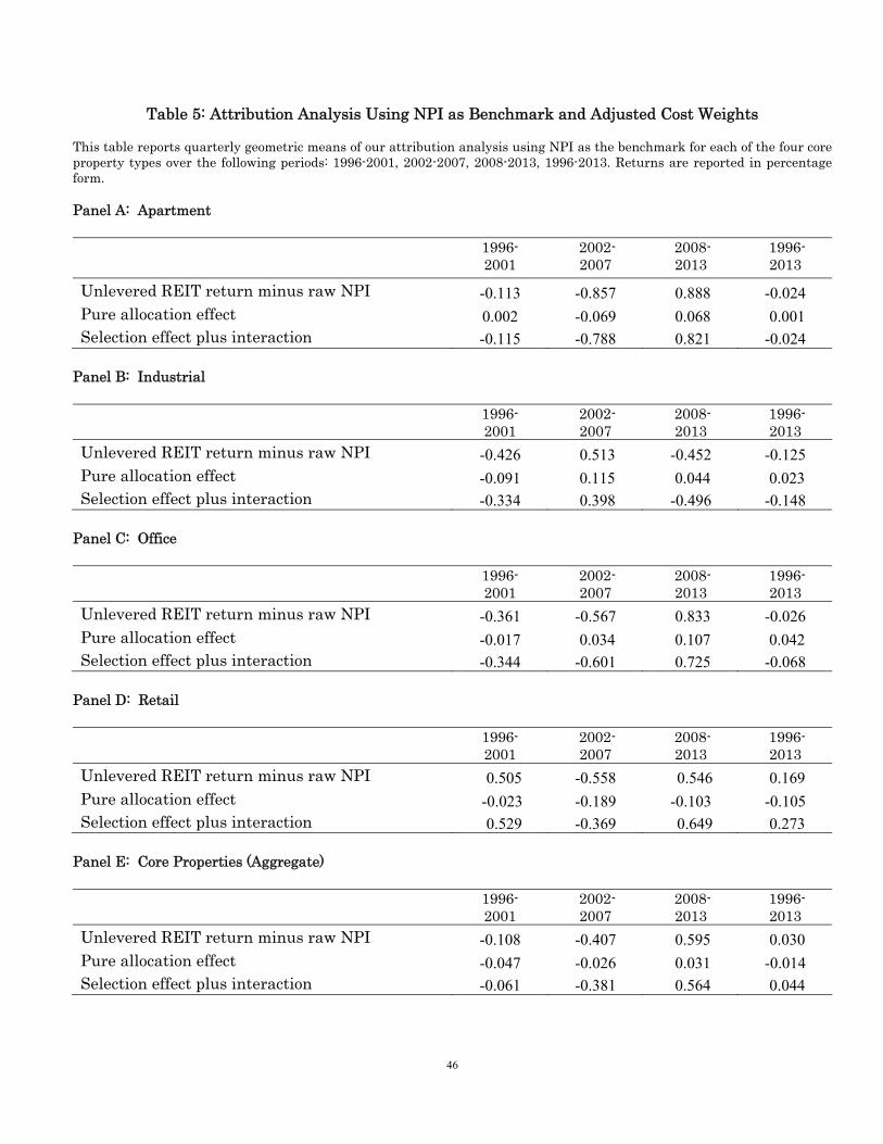
46

Table 5: Attribution Analysis Using NPI as Benchmark and Adjusted Cost Weights This table reports quarterly geometric means of our attribution analysis using NPI as the benchmark for each of the four core property types over the following periods: 1996-2001, 2002-2007, 2008-2013, 1996-2013. Returns are reported in percentage form. Panel A: Apartment 1996-

2001 2002- 2007

2008- 2013

1996- 2013

Unlevered REIT return minus raw NPI -0.113 -0.857 0.888 -0.024 Pure allocation effect 0.002 -0.069 0.068 0.001 Selection effect plus interaction -0.115 -0.788 0.821 -0.024

Panel B: Industrial 1996-

2001 2002- 2007

2008- 2013

1996- 2013

Unlevered REIT return minus raw NPI -0.426 0.513 -0.452 -0.125 Pure allocation effect -0.091 0.115 0.044 0.023 Selection effect plus interaction -0.334 0.398 -0.496 -0.148

Panel C: Office 1996-

2001 2002- 2007

2008- 2013

1996- 2013

Unlevered REIT return minus raw NPI -0.361 -0.567 0.833 -0.026 Pure allocation effect -0.017 0.034 0.107 0.042 Selection effect plus interaction -0.344 -0.601 0.725 -0.068

Panel D: Retail 1996-

2001 2002- 2007

2008- 2013

1996- 2013

Unlevered REIT return minus raw NPI 0.505 -0.558 0.546 0.169 Pure allocation effect -0.023 -0.189 -0.103 -0.105 Selection effect plus interaction 0.529 -0.369 0.649 0.273

Panel E: Core Properties (Aggregate) 1996-

2001 2002- 2007

2008- 2013

1996- 2013

Unlevered REIT return minus raw NPI -0.108 -0.407 0.595 0.030 Pure allocation effect -0.047 -0.026 0.031 -0.014 Selection effect plus interaction -0.061 -0.381 0.564 0.044

47

Table 6: Attribution Analysis Using NPI as Benchmark and Book Value Weights This table reports quarterly geometric means of our attribution analysis using NPI as the benchmark for each of the four core property types over the following periods: 1996-2001, 2002-2007, 2008-2013, 1996-2013. Returns are reported in percentage form. Panel A: Apartment 1996-

2001 2002- 2007

2008- 2013

1996- 2013

Unlevered REIT return minus raw NPI -0.113 -0.857 0.888 -0.024

Pure allocation effect -0.004 -0.065 0.062 -0.002

Selection effect plus interaction -0.109 -0.792 0.826 -0.022

Panel B: Industrial 1996-

2001 2002- 2007

2008- 2013

1996- 2013

Unlevered REIT return minus raw NPI -0.426 0.513 -0.452 -0.125

Pure allocation effect -0.073 0.096 0.060 0.028

Selection effect plus interaction -0.353 0.417 -0.512 -0.153

Panel C: Office 1996-

2001 2002- 2007

2008- 2013

1996- 2013

Unlevered REIT return minus raw NPI -0.361 -0.567 0.833 -0.026

Pure allocation effect 0.009 -0.020 0.113 0.035

Selection effect plus interaction -0.370 -0.547 0.720 -0.061

Panel D: Retail 1996-

2001 2002- 2007

2008- 2013

1996- 2013

Unlevered REIT return minus raw NPI 0.505 -0.558 0.546 0.169

Pure allocation effect -0.020 -0.172 -0.105 -0.099

Selection effect plus interaction 0.525 -0.386 0.651 0.267

Panel E: Core Properties (Aggregate) 1996-

2001 2002- 2007

2008- 2013

1996- 2013

Unlevered REIT return minus raw NPI -0.108 -0.407 0.595 0.030

Pure allocation effect -0.036 -0.046 0.033 -0.016

Selection effect plus interaction -0.072 -0.362 0.562 0.046

48

Table 7: Time Series Regression Analysis This table reports R-squared estimates obtained from regressing unlevered REIT return on our reweighted NPI index. We report results for the following periods: 1996-2001, 2002-2007, 2008-2013, 1996-2013. R-squared statistics are reported in percentage form. Panel A: Using Raw NPI 1996-

2001 2002- 2007

2008- 2013

1996- 2013

Apartment 0.0 9.6 17.3 11.7

Industrial 3.2 0.1 11.5 10.6

Office 0.0 0.0 7.0 4.4

Retail 24.2 0.3 13.2 6.1

Aggregate: Core 2.0 1.2 12.3 7.8

Panel B: Using Reweighted NPI 1996-

2001 2002- 2007

2008- 2013

1996- 2013

Apartment 0.0 12.5 17.6 12.3 Industrial 0.0 0.0 10.3 9.9 Office 0.0 0.1 10.0 5.9 Retail 20.9 2.3 12.4 6.9 Aggregate: Core 3.8 2.5 13.8 8.8

49

Table 8: Robustness Checks – 3 Year Estimation Periods This table reports average quarterly geometric means of our attribution analysis using NPI as the benchmark for each of the four core property types. We report results for the following periods: 1996-1998, 1999-2001, 2002-2004, 2005-2007, 2008-2010, and 2011-2013. Returns are reported in percentage form. Panel A: Apartment 1996-

1998 1999- 2001

2002- 2004

2005- 2007

2008- 2010

2011- 2013

Unlevered REIT return minus raw NPI -0.557 0.332 0.357 -2.072 3.340 -1.595 Pure allocation effect 0.029 -0.025 0.028 -0.167 0.049 0.087 Selection effect plus interaction -0.586 0.357 0.329 -1.905 3.290 -1.682

Panel B: Industrial 1996-

1998 1999- 2001

2002- 2004

2005- 2007

2008- 2010

2011- 2013

Unlevered REIT return minus raw NPI -0.673 -0.180 2.163 -1.141 0.373 -1.306 Pure allocation effect -0.242 0.058 0.263 -0.036 0.183 -0.100 Selection effect plus interaction -0.431 -0.239 1.900 -1.106 0.190 -1.206

Panel C: Office 1996-

1998 1999- 2001

2002- 2004

2005- 2007

2008- 2010

2011- 2013

Unlevered REIT return minus raw NPI -0.704 -0.021 1.107 -2.262 2.540 -0.915 Pure allocation effect -0.094 0.059 -0.067 0.138 0.140 0.073 Selection effect plus interaction -0.611 -0.080 1.174 -2.399 2.400 -0.989

Panel D: Retail 1996-

1998 1999- 2001

2002- 2004

2005- 2007

2008- 2010

2011- 2013

Unlevered REIT return minus raw NPI 0.753 0.259 0.646 -1.743 1.579 -0.511 Pure allocation effect 0.009 -0.055 -0.060 -0.317 -0.150 -0.055 Selection effect plus interaction 0.744 0.314 0.706 -1.426 1.729 -0.456

Panel E: Core 1996-

1998 1999- 2001

2002- 2004

2005- 2007

2008- 2010

2011- 2013

Unlevered REIT return minus raw NPI -0.279 0.063 1.073 -1.889 2.202 -1.048 Pure allocation effect -0.105 0.011 0.002 -0.055 0.041 0.021 Selection effect plus interaction -0.174 0.052 1.070 -1.834 2.161 -1.069

50

Table 9: Robustness Checks – Sample Period Dependence This table reports average quarterly geometric means of our attribution analysis using NPI as the benchmark for each of the four core property types. Returns are reported in percentage form. Panel A: Rolling 6 Year Windows

Apartment Industrial Office Retail Core

Unlevered REIT return minus raw NPI 0.093 0.004 -0.065 0.048 0.043

Pure allocation effect -0.017 0.084 0.035 -0.133 -0.013

Selection effect plus interaction 0.110 -0.079 -0.100 0.180 0.056

Panel B: Removing One Sample Year from Estimation

Apartment Industrial Office Retail Core

Unlevered REIT return minus raw NPI -0.022 -0.118 -0.025 0.159 0.027

Pure allocation effect 0.001 0.022 0.040 -0.099 -0.013

Selection effect plus interaction -0.023 -0.139 -0.065 0.258 0.040

51

Table 10: Attribution Analysis Using Property Subtypes – Retail Centers This table reports quarterly geometric means of our attribution analysis using NPI as the benchmark for the retail center subtype over the following periods: 1996-2001, 2002-2007, 2008-2013, 1996-2013. REITS classified as Shopping Center (property subtype 17) and Strip Centers (property subtype 18) and NCREIF properties classified as Community, Neighborhood and Power Centers constitute our definition of the retail center property subtype. Returns are reported in percentage form. 1996-

2001 2002- 2007

2008- 2013

1996- 2013

Unlevered REIT return minus raw NPI 0.358 -0.154 0.320 0.177 Pure allocation effect -0.013 -0.150 0.027 -0.045 Selection effect plus interaction 0.372 -0.004 0.293 0.221