PDF generated using the open source mwlib toolkit. See http://code.pediapress.com/ for more information.PDF generated at: Tue, 28 Apr 2015 19:24:47 CEST

GeoGebra ManualThe official manual of GeoGebra.

ContentsIntroduction 1Compatibility 2Installation Guide 3

Objects 5

Free, Dependent and Auxiliary Objects 5Geometric Objects 5Points and Vectors 5Lines and Axes 5Conic sections 5Functions 5Curves 6Inequalities 6Intervals 6General Objects 6Numbers and Angles 6Texts 6Boolean values 6Complex Numbers 7Lists 7Matrices 7Action Objects 7Selecting objects 7Change Values 7Naming Objects 7Animation 8Tracing 8Object Properties 8Labels and Captions 8Advanced Features 8Object Position 8Conditional Visibility 8Dynamic Colors 9LaTeX 9Layers 9Scripting 9

Tooltips 9

Tools 10

Tools 10Movement Tools 11Move Tool 11Record to Spreadsheet Tool 12Rotate around Point Tool 12Point Tools 12Point Tool 13Attach / Detach Point Tool 13Complex Number Tool 13Point on Object Tool 14Intersect Tool 14Midpoint or Center Tool 15Line Tools 15Line Tool 15Segment Tool 16Segment with Given Length Tool 16Ray Tool 16Vector from Point Tool 16Vector Tool 17Special Line Tools 17Best Fit Line Tool 17Parallel Line Tool 18Angle Bisector Tool 18Perpendicular Line Tool 18Tangents Tool 18Polar or Diameter Line Tool 19Perpendicular Bisector Tool 19Locus Tool 19Polygon Tools 20Rigid Polygon Tool 20Polyline Tool 20Regular Polygon Tool 21Polygon Tool 21Circle & Arc Tools 21Circle with Center and Radius Tool 22

Circle through 3 Points Tool 22Circle with Center through Point Tool 22Circumcircular Arc Tool 22Circumcircular Sector Tool 22Compass Tool 23Circular Sector Tool 23Semicircle through 2 Points Tool 23Circular Arc Tool 23Conic Section Tools 24Ellipse Tool 24Hyperbola Tool 24Conic through 5 Points Tool 24Parabola Tool 25Measurement Tools 25Distance or Length Tool 25Angle Tool 26Slope Tool 26Area Tool 26Angle with Given Size Tool 27Transformation Tools 27Translate by Vector Tool 27Reflect about Line Tool 28Reflect about Point Tool 28Rotate around Point Tool 28Reflect about Circle Tool 28Dilate from Point Tool 29Special Object Tools 29Image Tool 29Pen Tool 30Slider Tool 31Relation Tool 32Function Inspector Tool 32Text Tool 32Action Object Tools 33Check Box Tool 33Input Box Tool 33Button Tool 34General Tools 34

Custom Tools 34Show / Hide Label Tool 35Zoom Out Tool 35Zoom In Tool 35Delete Tool 36Move Graphics View Tool 36Show / Hide Object Tool 37Copy Visual Style Tool 37

Commands 38

Commands 38Geometry Commands 38AffineRatio Command 39Angle Command 39AngleBisector Command 41Arc Command 41Area Command 42Centroid Command 42CircularArc Command 43CircularSector Command 43CircumcircularArc Command 43CircumcircularSector Command 44Circumference Command 44ClosestPoint Command 44CrossRatio Command 45Direction Command 45Distance Command 45Intersect Command 46IntersectPath Command 47Length Command 48Line Command 49PerpendicularBisector Command 49Locus Command 50Midpoint Command 50PerpendicularLine Command 51Perimeter Command 52Point Command 52PointIn Command 53

Polyline Command 53Polygon Command 53Radius Command 54Ray Command 54RigidPolygon Command 54Sector Command 55Segment Command 55Slope Command 56Tangent Command 56Vertex Command 57Algebra Commands 57Div Command 58Expand Command 59Factor Command 59GCD Command 60LCM Command 61Max Command 62Min Command 63Mod Command 64PrimeFactors Command 64Simplify Command 65Text Commands 65FractionText Command 66FormulaText Command 66LetterToUnicode Command 67Ordinal Command 67RotateText Command 67TableText Command 68Text Command 69TextToUnicode Command 70UnicodeToLetter Command 70UnicodeToText Command 70VerticalText Command 71Logic Commands 71CountIf Command 71IsDefined Command 72If Command 72IsInRegion Command 73

IsInteger Command 73KeepIf Command 73Relation Command 74Functions & Calculus Commands 74Asymptote Command 75Coefficients Command 76CompleteSquare Command 77ComplexRoot Command 77Curvature Command 78CurvatureVector Command 78Curve Command 78Degree Command 79Denominator Command 79Derivative Command 80Extremum Command 81Factors Command 81Function Command 82ImplicitCurve Command 83Integral Command 83IntegralBetween Command 84Intersect Command 85Iteration Command 86IterationList Command 87LeftSum Command 87Limit Command 87LimitAbove Command 88LimitBelow Command 89LowerSum Command 90Numerator Command 90OsculatingCircle Command 91PartialFractions Command 91PathParameter Command 92Polynomial Command 92RectangleSum Command 93Root Command 93RootList Command 94Roots Command 94SolveODE Command 94

TaylorPolynomial Command 96TrapezoidalSum Command 97InflectionPoint Command 97UpperSum Command 97Conic Commands 98Asymptote Command 99Axes Command 99Center Command 100Circle Command 100Conic Command 101ConjugateDiameter Command 101Directrix Command 102Eccentricity Command 102Ellipse Command 102LinearEccentricity Command 103MajorAxis Command 103SemiMajorAxisLength Command 103Focus Command 104Hyperbola Command 104Incircle Command 105Parabola Command 105Parameter Command 105Polar Command 105MinorAxis Command 106SemiMinorAxisLength Command 106Semicircle Command 106List Commands 107Append Command 108Classes Command 108Element Command 109First Command 110Frequency Command 111IndexOf Command 112Insert Command 113Intersect Command 113Intersection Command 115IterationList Command 115Join Command 115

Last Command 116OrdinalRank Command 117PointList Command 117Product Command 117RandomElement Command 118RemoveUndefined Command 119Reverse Command 119RootList Command 120SelectedElement Command 120SelectedIndex Command 120Sequence Command 120Sort Command 121Take Command 122TiedRank Command 123Union Command 123Unique Command 123Zip Command 124Vector & Matrix Commands 124ApplyMatrix Command 125CurvatureVector Command 125Determinant Command 126Identity Command 126Invert Command 127PerpendicularVector Command 128ReducedRowEchelonForm Command 129Transpose Command 129UnitPerpendicularVector Command 130UnitVector Command 131Vector Command 132Transformation Commands 132Dilate Command 133Reflect Command 133Rotate Command 134Shear Command 134Stretch Command 134Translate Command 135Chart Commands 135BarChart Command 135

BoxPlot Command 136DotPlot Command 137FrequencyPolygon Command 137Histogram Command 138HistogramRight Command 139NormalQuantilePlot Command 139ResidualPlot Command 140StemPlot Command 140Statistics Commands 141ANOVA Command 142Classes Command 142Covariance Command 143Fit Command 144FitExp Command 144FitGrowth Command 145FitLineX Command 145FitLine Command 146FitLog Command 146FitLogistic Command 147FitPoly Command 147FitPow Command 148FitSin Command 148Frequency Command 149FrequencyTable Command 150GeometricMean Command 151HarmonicMean Command 151Mean Command 151MeanX Command 152MeanY Command 152Median Command 152Mode Command 153CorrelationCoefficient Command 153Percentile Command 153Q1 Command 154Q3 Command 154RSquare Command 155RootMeanSquare Command 155SD Command 155

SDX Command 156SDY Command 156Sxx Command 156Sxy Command 156Syy Command 157Sample Command 157SampleSD Command 158SampleSDX Command 158SampleSDY Command 159SampleVariance Command 159Shuffle Command 160SigmaXX Command 160SigmaXY Command 161SigmaYY Command 161Spearman Command 161Sum Command 162SumSquaredErrors Command 163TMean2Estimate Command 163TMeanEstimate Command 164TTest Command 164TTest2 Command 165TTestPaired Command 165Variance Command 166Probability Commands 166Bernoulli Command 167BinomialCoefficient Command 167BinomialDist Command 168Cauchy Command 169ChiSquared Command 170Erlang Command 171Exponential Command 172FDistribution Command 172Gamma Command 173HyperGeometric Command 174InverseBinomial Command 175InverseCauchy Command 175InverseChiSquared Command 175InverseExponential Command 176

InverseFDistribution Command 176InverseGamma Command 176InverseHyperGeometric Command 177InverseNormal Command 177InversePascal Command 177InversePoisson Command 178InverseTDistribution Command 178InverseWeibull Command 178InverseZipf Command 178LogNormal Command 179Logistic Command 180Normal Command 181Pascal Command 182Poisson Command 183RandomBetween Command 184RandomBinomial Command 185RandomNormal Command 185RandomPoisson Command 186RandomUniform Command 186TDistribution Command 187Triangular Command 188Uniform Command 189Weibull Command 189Zipf Command 190Spreadsheet Commands 191Cell Command 191CellRange Command 192Column Command 192ColumnName Command 192FillCells Command 193FillColumn Command 193FillRow Command 194Row Command 194Scripting Commands 194Button Command 195Checkbox Command 196CopyFreeObject Command 196Delete Command 196

Execute Command 197GetTime Command 197HideLayer Command 198Pan Command 198ParseToFunction Command 198ParseToNumber Command 199Plane Command 199PlaySound Command 200Rename Command 201SelectObjects Command 201SetActiveView Command 202SetAxesRatio Command 202SetBackgroundColor Command 202SetCaption Command 203SetColor Command 203SetConditionToShowObject Command 204SetCoords Command 205SetDynamicColor Command 205SetFilling Command 205SetFixed Command 206SetLabelMode Command 206SetLayer Command 206SetLineStyle Command 207SetLineThickness Command 207SetPointSize Command 207SetPointStyle Command 208SetTooltipMode Command 208SetValue Command 209SetVisibleInView Command 209ShowLabel Command 209ShowLayer Command 210Slider Command 210StartAnimation Command 211InputBox Command 211UpdateConstruction Command 212ZoomIn Command 212ZoomOut Command 213Discrete Math Commands 213

ConvexHull Command 214DelaunayTriangulation Command 214Hull Command 214MinimumSpanningTree Command 214ShortestDistance Command 215TravelingSalesman Command 215Voronoi Command 215GeoGebra Commands 215AxisStepX Command 216AxisStepY Command 216ClosestPoint Command 216ConstructionStep Command 217Corner Command 217DynamicCoordinates Command 218Name Command 219Object Command 219SlowPlot Command 219ToolImage Command 220Optimization Commands 220Maximize Command 220Minimize Command 220CAS Specific Commands 221CFactor Command 223CSolutions Command 224CSolve Command 225CommonDenominator Command 226Cross Command 226Dimension Command 227Division Command 227Divisors Command 228DivisorsList Command 228DivisorsSum Command 229Dot Command 229ImplicitDerivative Command 230IsPrime Command 230LeftSide Command 231MatrixRank Command 232MixedNumber Command 232

NIntegral Command 233NSolutions Command 233NSolve Command 234NextPrime Command 235Numeric Command 235PreviousPrime Command 236RandomPolynomial Command 236Rationalize Command 237RightSide Command 237Solutions Command 238Solve Command 239Substitute Command 240ToComplex Command 240ToExponential Command 241ToPoint Command 241ToPolar Command 242nPr Command 242Predefined Functions and Operators 243

User interface 245

Views 245Graphics View 247Customizing the Graphics View 249Algebra View 251Spreadsheet View 253CAS View 256Probability Calculator 260Construction Protocol 261Input Bar 262Menubar 263Toolbar 264Navigation Bar 266File Menu 266Edit Menu 268View Menu 270Perspectives 272Options Menu 273Tools Menu 274

Window Menu 275Help Menu 275Context Menu 276Customize the Settings 276Export Graphics Dialog 277Export Worksheet Dialog 278Properties Dialog 278Redefine Dialog 279Tool Creation Dialog 280Keyboard Shortcuts 281Settings Dialog 285Virtual Keyboard 286Tool Manager Dialog 287Accessibility 287

Publishing 288

Creating Pictures of the Graphics View 288Upload to GeoGebraTube 289Export as html Webpage 289Embedding to CMS, VLE (Moodle) and Wiki 290Export to LaTeX (PGF, PSTricks) and Asymptote 291Printing Options 292

ReferencesArticle Sources and Contributors 293Image Sources, Licenses and Contributors 305

Article LicensesLicense 309

Introduction 1

Introduction

Tutorials

Step-by-step tutorials for GeoGebra both for beginners and experts

Forum [1]

Get quick answers to all your questions in our friendly GeoGebra User Forum [1]

GeoGebra Manual

The GeoGebra Manual describes all commands and tools of our software

Events [2]

Visit GeoGebra Events [3] near to you with workshops and presentations

Compatibility 2

CompatibilityGeoGebra is backward compatible in sense that files created with older version should open in later versions.Sometime we make changes which will cause files to behave differently.Differences from GeoGebra 4.4 to 5.0• The winding rule [1] for self-intersecting polygons has changed so they will look different.Differences from GeoGebra 3.2 to 4.0•• lists of angles, integrals, barcharts, histograms etc. are now visible•• lists {Segment[A,B], Segment[B,C] } are now draggable•• circle with given radius (e.g. Circle[(1,1),2]) draggable•• Distance[ Point, Segment ] gives distance to the Segment (was to the extrapolated line in 3.2)•• Angle[A,B,C] now resizes if B is too close to A or C•• Integral[function f,function g,a,b] is now transcribed to IntegralBetween[function f,function g,a,b].•• Objects that are a translation by a free vector are now draggable, eg Translate[A, Vector[(1,1)]]•• Points on paths may behave differently when the path is changed, e.g. point on conic.

LaTeX EquationsThe LaTeX rendering is now nicer, but some errors in LaTeX syntax which were ignored in 3.2 will cause missingtexts in 4.0.• Make sure that each \left\{ has corresponding \right..• See here for more tips about getting LaTeX working: http:/ / forum. geogebra. org/ viewtopic. php?f=20&

t=33449

Installation Guide 3

Installation Guide

GeoGebra Installation•• Installation•• Mass Installation•• FAQ

WindowsGeoGebra can be installed for Windows in two ways:• GeoGebra Installer for Windows [1] (recommended)• GeoGebra Portable for Windows [2] (runs from USB memory sticks for example)Please note that the Installer will automatically update to newer versions.

MacOS XWe provide GeoGebra in two ways for Mac OS X:• GeoGebra in the Mac App Store [3] (recommended)• GeoGebra Portable for OSX [4].Please note that the Mac App Store will automatically update to newer versions.

LinuxThe following GeoGebra Linux installers are available:• 64 bit [5] / 32 bit [6] installers for .deb based systems (Debian, Ubuntu)• 64 bit [7] / 32 bit [8] installers for .rpm based systems (Red Hat, openSUSE)• Portable Linux [9] bundle for 64 and 32 bit Linux systems

RepositoryThe .deb and .rpm installers will automatically add the official GeoGebra repository to the package managementsystem on the workstation. This will enable automatic update of GeoGebra every time a new version is released.Note that the portable version will not automatically update.If you want to include GeoGebra in your custom Linux distribution with GeoGebra included, the best way is to addthe official GeoGebra repository (http:/ / www. geogebra. net/ linux/ ) to your package management system. TheGPG key of the repository is at http:/ / www. geogebra. net/ linux/ office@geogebra. org. gpg. key. The name of thepackage is geogebra5. This will conflict with the earlier versions (4.0, 4.2 and 4.4), which are named geogebra (andgeogebra44 for 4.4) and should be deleted first.

All versions

Installation Guide 4

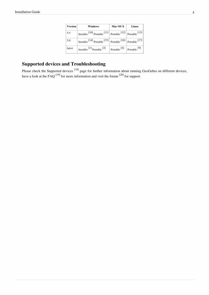
Version Windows Mac OS X Linux

4.4 Installer [10] Portable [11] Portable [12] Portable [13]

5.0 Installer [14] Portable [15] Portable [16] Portable [17]

latest Installer [1] Portable [2] Portable [4] Portable [9]

Supported devices and TroubleshootingPlease check the Supported devices [18] page for further information about running GeoGebra on different devices,have a look at the FAQ [19] for more information and visit the forum [20] for support.

5

Objects

Free, Dependent and Auxiliary Objects

Geometric Objects

Points and Vectors

Lines and Axes

Conic sections

Functions

Curves 6

Curves

Inequalities

Intervals

General Objects

Numbers and Angles

Texts

Boolean values

Complex Numbers 7

Complex Numbers

Lists

Matrices

Action Objects

Selecting objects

Change Values

Naming Objects

Animation 8

Animation

Tracing

Object Properties

Labels and Captions

Advanced Features

Object Position

Conditional Visibility

Dynamic Colors 9

Dynamic Colors

LaTeX

Layers

Scripting

Tooltips

10

Tools

ToolsGeoGebra’s Tools enable you to produce new Objects using your pointing device. They can be activated by clickingon the corresponding buttons of the Toolbar.Note: All Tools have their Commands equivalents which are suitable for more complicated constructions.

Different Toolbars for Different ViewsEach View except the Algebra View has its own Toolbar, providing Tools specific for the View you are workingwith.• Graphics View Toolbar• 3D Graphics View Toolbar• CAS View Toolbar• Spreadsheet View Toolbar

Once you start using another View within the GeoGebra window, the Toolbar changes automatically. If you openanother View in a separate window, it will have its Toolbar attached.

ToolboxesEach Toolbar is divided into Toolboxes, containing one or more related Tools. You may open a Toolbox by clicking• on one of the default Tools in the Toolbar (GeoGebra Web and Tablet Apps)• on the little arrow in the lower right corner of the default Tools (GeoGebra Desktop).You can reorder these Toolboxes and save the setting in the GeoGebra Worksheet (*.ggb). See Customizing theToolbar for details.

More Information about ToolsFor more information please check our complete list of all available Tools as well as the general information aboutToolbars, creating Custom Tools and Customizing the Toolbar.

Movement Tools 11

Movement Tools

Movement tools are by default grouped under icon (the first from left) in the toolbar. Currently there are threemovement tools:•• Move•• Rotate around Point•• Record to Spreadsheet

Move Tool

Move Tool in the Graphics ViewDrag and drop Free Objects with the mouse. If you select an object by clicking on it in Move mode, you may…• … delete the object by pressing the Delete key• … move the object by using the arrow keys (see section Manual Animation)

Note:You can quickly activate the Move Tool by pressing the Esc key of your keyboard.To move a SliderToolSlider when Move Tool is selected, you need to drag it with your right mouse button.

Move Tool in the 3D Graphics ViewUsing the Move Tool in the 3D Graphics View you may drag and drop free points. In order to move a point in thethree-dimensional coordinate system, you can switch between two modes by clicking on the point:• Mode x-y-plane: You may move the point parallel to the x-y-plane without changing the z-coordinate.• Mode z-axis: You may move the point parallel to the z-axis without changing the x- and y-coordinates.

Record to Spreadsheet Tool 12

Record to Spreadsheet ToolThis tool allows you to move an object and to record a sequence of its values in the Spreadsheet View. This toolworks for numbers, points, and vectors.Note: GeoGebra will use the first two empty columns of the Spreadsheet View to record the values of the selectedobjects.

Rotate around Point ToolSelect the object you want to rotate. Then, click on a point to specify the center of rotation and enter therotation angle into the text field of the appearing dialog window.Note: See also Rotate command.

Point Tools

Point tools are by default grouped under icon (the second from the left) in the toolbar. Currently there are sixpoint tools:•• Point•• Point on Object•• Intersect•• Midpoint or Centre•• Attach / Detach Point•• Complex Number

Point Tool 13

Point ToolClick on the drawing pad in the Graphics View in order to create a new point. The coordinates of the point arefixed when the mouse button is released.Note:By clicking on a segment (or interval), straight line, polygon, conic section, function, or curve you cancreate a point on this object (see also Point CommandPoint command). Clicking on the intersection of twoobjects creates this intersection point (see also Intersect ToolIntersect tool and Intersect CommandIntersectcommand).

Attach / Detach Point ToolTo attach a point to a path or region click a free point and the path or region. From now on, the point can still be

moved via Move Tool, but only within the path or region.To detach a point that is defined as point on path or region simply click the point. The point will become free.Note: You can also use Point Command and PointIn Command for attaching a point. See also CopyFreeObjectCommand.

Complex Number ToolClick in the the Graphics View in order to create a new complex number. The value of the complex numberpoint is fixed when the mouse button is released.

Point on Object Tool 14

Point on Object ToolTo create a point, which is fixed to an object, click on the tool button first and then on the object. This new point can

be moved via Move Tool, but only within the object.Note: To put a point in the interior of a Circle or Ellipse you will need to increase the Opacity from 0 first. If youclick on the perimeter of an object (eg Circle, Ellipse, Polygon), then the point will be fixed to the perimeter ratherthan the interior.

Intersect ToolIntersection points of two objects can be created in two ways (see also Intersect command).

•• Selecting two objects creates all intersection points (if possible).• Directly clicking on an intersection of the two objects creates only this single intersection point.

Note: Sometimes it's useful to display only the portions of the intersecating objects near the intersection point.To do so, right click on the intersection point, and check the option Show trimmed intersection lines in theBasic tab of the Properties dialog of the object, then hide the intersecting objects.

Outlying IntersectionsFor segments, rays, or arcs you may specify whether you want to Allow outlying intersections on tab Basic of theProperties Dialog. This can be used to get intersection points that lie on the extension of an object. For example, theextension of a segment or a ray is a straight line.

Midpoint or Center Tool 15

Midpoint or Center ToolYou may click on either two points or one segment to get its midpoint. You can also click on a conic section (circleor ellipse) in order to create its center point.See also Center ( , : Centre) and Midpoint commands.

Line Tools

Line tools are by default grouped under icon (the third from left) in the toolbar. Currently there are seven linetools:•• Line•• Segment•• Segment with Given Length•• Ray•• Polyline•• Vector•• Vector from Point

Line ToolSelecting two points A and B creates a straight line through A and B.Notes:The line’s direction vector is \overrightarrow{AB}, (B - A)See also Line CommandLine command.

Segment Tool 16

Segment ToolSelect two points A and B in order to create a segment between A and B (see also Segment command).Note: In the Algebra View, the segment's length is displayed.

Segment with Given Length ToolClick on a point A that should be the starting point of the segment. Specify the desired length a of the segmentin the appearing window (see also Segment command).Note: This tool creates a segment with length a and endpoint B which may be rotated around the starting pointA by using tool Move.

Ray ToolSelecting two points A and B creates a ray starting at A through B (see also Ray command).Note: In the Algebra View the equation of the corresponding line is displayed.

Vector from Point ToolSelect a point A and a vector v to create the new point B = A + v as well as the vector from A to B (see alsoVector command).

Vector Tool 17

Vector ToolSelect the starting point and then the end point of the vector (see also Vector command).

Special Line Tools

Special line tools are by default grouped under icon (the fourth from the left) in the toolbar. Currently there areeight line tools:•• Perpendicular Line•• Parallel Line•• Perpendicular Bisector•• Angle Bisector•• Tangents•• Polar or Diameter Line•• Best Fit Line•• Locus

Best Fit Line ToolCreates the best fit line for a set of points, chosen as follows :

• Creating a selection rectangle that contains all points.• Selecting a list of points .

Note: See also FitLine command.

Parallel Line Tool 18

Parallel Line ToolSelecting a line g and a point A defines a straight line through A parallel to g (see also Line command ).Note: The line’s direction is the direction of line g.

Angle Bisector ToolAngle bisectors can be defined in two ways:

• Selecting three points A, B, and C produces the angle bisector of the enclosed angle, where point B is the apex.•• Selecting two lines produces their two angle bisectors.

Notes:The direction vectors of all angle bisectors have length 1 See also AngleBisector CommandAngleBisectorcommand.

Perpendicular Line ToolSelecting a line (or a segment) g and a point A creates a straight line through A perpendicular to line (orsegment) g (see also PerpendicularLine command).Note: The line’s direction is equivalent to the perpendicular vector of g (see also PerpendicularVectorcommand).

Tangents ToolTangents to a conic section can be produced in several ways (see also Tangent command):

• Selecting a point A and a conic c produces all tangents through A to c.• Selecting a line g and a conic c produces all tangents to c that are parallel to line g.• Selecting a point A and a function f produces the tangent line to f in x = x(A).• Selecting two circles c and d produces the common tangents to the two circles (up to 4).

Note: x(A) represents the x-coordinate of point A. If point A lies on the function graph, the tangent runsthrough point A.Note: Type rather than if you want a conic (parabola) rather than a function.

Polar or Diameter Line Tool 19

Polar or Diameter Line ToolThis tool creates the polar or diameter line of a conic section (see also Polar command).

•• Select a point and a conic section to get the polar line.•• Select a line or a vector and a conic section to get the diameter line.

Perpendicular Bisector ToolClick on either a segment (or interval) s or two points A and B in order to create a perpendicular bisector.

Notes:The bisector’s direction is equivalent to the perpendicular vector of segment (or interval) s or ABSee alsoPerpendicularVector CommandPerpendicularVector command See also PerpendicularBisectorCommandPerpendicularBisector command.

Locus ToolSelect a point B that depends on another point A and whose locus should be drawn. Then, click on point A tocreate the locus of point B (see also Locus command).Note: Point A has to be a point on an object (e. g. line, segment/interval, circle).Example:Type f(x) = x^2 – 2 x – 1 into the Input Bar and press the Enter-key. Place a new point A on thex-axis (see Point ToolPoint tool; see Point CommandPoint command). Create point B = (x(A), f'(x(A))) thatdepends on point A. Select tool and successively click on point B and point A.Drag point A along the x-axis tosee point B moving along its locus line.

Warning: Locus is undefined, if the dependent point depends on Point Command with two parameters or PathParameter Command.

Polygon Tools 20

Polygon Tools

Polygon tools are by default grouped under icon (the fifth from the left) in the toolbar. Currently there are fourpolygon tools:•• Polygon•• Regular Polygon•• Rigid Polygon•• Vector Polygon

Rigid Polygon ToolSuccessively select at least three free points which will be the vertices of the polygon. Then, click the firstpoint again in order to close the polygon. The resulting polygon will keep the shape: you can move it androtate it by moving two vertices.Holding down the Alt key when drawing a rigid polygon allows to get angles that are a multiple of 15°.

Notes:The polygon's area is displayed in the Algebra View. See also RigidPolygon CommandRigid Polygoncommand.

Polyline ToolSuccessively select at least two points which will be the vertices of the polyline.Holding down the Alt key when drawing a Polyline allows to get angles that are a multiple of 15°.

Note: In the Algebra View, the polyline length is displayed.

Regular Polygon Tool 21

Regular Polygon ToolSelect two points A and B and specify the number n of vertices in the input field of the appearing dialogwindow. This gives you a regular polygon with n vertices including points A and B.Note: See also Polygon command.

Polygon ToolSuccessively select at least three points which will be the vertices of the polygon. Then, click the first pointagain in order to close the polygon.Holding down the Alt key when drawing a Polygon allows to get angles that are a multiple of 15°.Notes:The polygon area is displayed in the Algebra View. See also Polygon CommandPolygon command.

Circle & Arc Tools

Circle and arc tools are by default grouped under icon (the sixth from the left) in the toolbar. Currently thereare nine circle and arc tools:•• Circle with Centre through Point•• Circle with Centre and Radius•• Compasses•• Circle through 3 Points•• Semicircle through 2 Points•• Circular Arc•• Circumcircular Arc•• Circular Sector•• Circumcircular Sector

Circle with Center and Radius Tool 22

Circle with Center and Radius ToolSelect the center point M and enter the radius in the text field of the appearing dialog window.Note: See also Circle command.

Circle through 3 Points ToolSelecting three points A, B, and C defines a circle through these points (see also Circle command).Note: If the three points lie on the same line, the circle degenerates to this line.

Circle with Center through Point ToolSelecting a point M and a point P defines a circle with center M through P.

Circumcircular Arc ToolSelect three points A, B, and C to create a circular arc through these points. Thereby, point A is the startingpoint of the arc, point B lies on the arc, and point C is the endpoint of the arc.Note: See also CircumcircularArc command.

Circumcircular Sector ToolSelect three points A, B, and C to create a circular sector through these points. Thereby, point A is the startingpoint of the sector’s arc, point B lies on the arc, and point C is the endpoint of the sector’s arc.Note: See also CircumcircularSector command.

Compass Tool 23

Compass ToolSelect a segment or two points to specify the radius. Then, click on a point that should be the center of the newcircle.

Circular Sector ToolFirst, select the center point M of the circular sector. Then, select the starting point A of the sector’s arc, beforeyou select a point B that specifies the length of the sector’s arc.Notes:While point A always lies on the sector’s arc, point B does not have to lie on it.See also CircularSectorCommandCircularSector command.

Semicircle through 2 Points ToolSelect two points A and B to create a semicircle above the segment (or interval) AB.Note: See also Semicircle command.

Circular Arc ToolFirst, select the center point M of the circular arc. Then, select the starting point A of the arc, before you selecta point B that specifies the length of the arc.Notes:While point A always lies on the circular arc, point B does not have to lie on it.See also CircularArcCommandCircularArc command.

Conic Section Tools 24

Conic Section Tools

Conic section tools are by default grouped under icon (the sixth from the right) in the toolbar. Currently thereare four conic section tools:•• Ellipse•• Hyperbola•• Parabola•• Conic through 5 Points

Ellipse ToolSelect the two foci of the ellipse. Then, specify a third point that lies on the ellipse.Note: See also Ellipse command.

Hyperbola ToolSelect the two foci of the hyperbola. Then, specify a third point that lies on the hyperbola.Note: See also Hyperbola command.

Conic through 5 Points ToolSelecting five points produces a conic section through these points.Notes:If four of these five points lie on a line, the conic section is not defined. See also Conic CommandConiccommand.

Parabola Tool 25

Parabola ToolSelect a point (focus) and the directrix of the parabola, in any order.Note:

•• If you select the directrix line first, a preview of the resulting parabola is shown.• See also Parabola command.

Measurement Tools

Measurement tools are by default grouped under icon (the fifth from the right) in the toolbar. Currently thereare six measurement tools:•• Angle•• Angle with Given Size•• Distance or Length•• Area•• Slope•• Create List

Distance or Length ToolThis tool returns the distance between two points, two lines, or a point and a line as a number, and shows adynamic text in the Graphics View. It can also be used to measure the length of a segment (or interval), thecircumference of a circle, or the perimeter of a polygon.Note: See also Distance and Length commands.

Angle Tool 26

Angle ToolWith this tool you can create angles in different ways:

•• Click on three points to create an angle between these points. The second point selected is the vertex of theangle.

•• Click on two segments to create the angle between them.•• Click on two lines to create the angle between them.•• Click on two vectors to create the angle between them.•• Click on a polygon to create all angles of this polygon.

Notes:If the polygon was created by selecting its vertices in counter clockwise orientation, the Angle tool gives youthe interior angles of the polygonAngles are created in counter clockwise orientation. Therefore, the order ofselecting these objects is relevant for the Angle tool. If you want to limit the maximum size of an angle to 180°,un-check Allow Reflex Angle on tab Basic of the Properties DialogSee also Angle CommandAngle command.

Slope ToolThis tool gives you the slope of a line and shows a slope triangle in the Graphics View, whose size may bechanged using Properties Dialog (see also Slope command).

Area ToolThis tool gives you the area of a polygon, circle, or ellipse as a number and shows a dynamic text in theGraphics View.

Note: See also Area command.

Angle with Given Size Tool 27

Angle with Given Size ToolSelect two points A and B and type the angle’s size into the text field of the appearing window.

Notes:This tool creates a point C and an angle α, where α is the angle ABCSee also Angle CommandAnglecommand

Transformation Tools

Transformation tools are by default grouped under icon (the fourth from the right) in the toolbar. Currentlythere are six transformation tools:•• Reflect about Line•• Reflect about Point•• Reflect about Circle•• Rotate around Point•• Translate by Vector•• Dilate from Point

Translate by Vector ToolSelect the object you want to translate. Then, click on the translation vector or click twice to make a vector(see also Translate command).

From version 4.0.15.0 you can also now just drag to clone an object with this tool.

Reflect about Line Tool 28

Reflect about Line ToolSelect the object you want to reflect. Then, click on a line to specify the mirror/line of reflection (see alsoReflect command).

Reflect about Point ToolSelect the object you want to reflect. Then, click on a point to specify the mirror/point of reflection (see alsoReflect command).

Rotate around Point ToolSelect the object you want to rotate. Then, click on a point to specify the center of rotation and enter therotation angle into the text field of the appearing dialog window.Note: See also Rotate command.

Reflect about Circle ToolInverts a geometric object about a circle. Select the object you want to invert. Then, click on a circle to specifythe mirror/circle of inversion.Note: See also Reflect command.

Dilate from Point Tool 29

Dilate from Point ToolSelect the object to be dilated. Then, click on a point to specify the dilation center and enter the dilation factorinto the text field of the appearing dialog window (see also Dilate command).

Special Object Tools

Special object tools are by default grouped under icon (the third from the right) in the toolbar. Currently thereare six special object tools:•• Text•• Image•• Pen Tool•• Relation•• Probability Calculator•• Function Inspector

Image ToolThis tool allows you to insert an image into the Graphics View.First, specify the location of the image in one of the following two ways:• Click in the Graphics View to specify the position of the image’s lower left corner.•• Click on a point to specify this point as the lower left corner of the image.Then, a file-open dialog appears that allows you to select the image file from the files saved on your computer.

Note: After selecting the tool Insert Image, you can use the keyboard shortcut Alt-click in order to paste animage directly from your computer’s clipboard into the Graphics View.Note: Transparent [GIF [1]] and [PNG [2]] files are supported, but for PNGs you may need to edit them first so thatthey have an alpha channel (for example using [IrfanView [3]], save using the PNGOUT plugin and chooseRGB+Alpha)

Properties of ImagesThe position of an image may be absolute on screen or relative to the coordinate system. You can specify this on tabBasic of the Properties Dialog of the image.You may specify up to three corner points of the image on tab Position of the Properties Dialog. This gives you theflexibility to scale, rotate, and even distort images (see also Corner command).•• Corner 1: position of the lower left corner of the image•• Corner 2: position of the lower right corner of the image

Note: This corner may only be set if Corner 1 was set before. It controls the width of the image.•• Corner 4: position of the upper left corner of the image

Note: This corner may only be set if Corner 1 was set before. It controls the height of the image.Example: Create three points A, B, and C to explore the effects of the corner points.Set point A as the first and point B as the second corner of your image. By dragging points A and B in Move mode you can explore their influence.

Image Tool 30

Now, remove point B as the second corner of the image. Set point A as the first and point C as the fourth corner andexplore how dragging the points now influences the image. Finally, you may set all three corner points and see howdragging the points distorts your image.Example: In order to attach your image to a point A, and set its width to 3 and its height to 4 units, you could do thefollowing:Set Corner 1 to A Set Corner 2 to A + (3, 0) Set Corner 4 to A + (0, 4)

Note: If you now drag point A in Move mode, the size of your image does not change.You may specify an image as a Background image on tab Basic of the Properties Dialog. A background image liesbehind the coordinate axes and cannot be selected with the mouse any more.Note: In order to change the background setting of an image, you may open the Properties Dialog by selecting Properties… from the Edit Menu.The Transparency of an image can be changed in order to see objects or axes that lie behind the image. You can setthe transparency of an image by specifying a Filling value between 0 % and 100 % on tab Style of the PropertiesDialog.

Pen ToolThe Pen Tool allows the user to add freehand notes and drawings to the Graphics View. This makes the Pen Toolparticularly useful when using GeoGebra for presentations or with multimedia interactive whiteboards. To add afreehand note onto a region of the Graphics View, start drawing while keeping the left button of the mouse pressed.Release the mouse button to finish.GeoGebra stores the notes you traced in the Graphic View as a polyline (assigning the name stroke to it), so you canapply to it any operation applicable to the related object (move, rotate, delete, etc.).The default colour of the pen is black, but you can change the pen properties (colour, style, and thickness) using theStyling Bar, selecting the black triangle icon displayed on the Graphics View title bar.

ErasingTo erase a portion of your notes created in the Graphic View with the Pen Tool, press and hold the right mousebutton while moving it on the notes you want to delete. Release the mouse button to finish.In order to delete the stroke you previously created, erase it totally, or use the context menu of the object, or justdelete the corresponding item in Algebra View.

Slider Tool 31

Slider ToolClick on any free place in the Graphics View to create a slider for a number or an angle. The appearing dialogwindow allows you to specify the Name, Interval [min, max], and Increment of the number or angle, as well as theAlignment and Width of the slider (in pixels), and its Speed and Animation modality.Note: In the Slider dialog window you can enter a degree symbol ° or pi (π) for the interval and increment by usingthe following keyboard shortcuts:Alt-O (Mac OS: Ctrl-O) for the degree symbol ° Alt-P (Mac OS: Ctrl-P) for the pisymbol πThe position of a slider may be absolute in the Graphics View (this means that the slider is not affected by zooming,but always remains in the visible part of the Graphics View) or relative to the coordinate system (see PropertiesDialog of the corresponding number or angle).Note:In GeoGebra, a slider is the graphical representation of a Numbers and Angles#Free Numbers and Anglesfreenumber or free angle. You can easily create a slider for any existing Numbers and Angles#Free Numbers andAnglesfree number or angle by showing this object in the Graphics View (see Context Menu; see tool Show / HideObject ToolShow/Hide Object).

Fixed sliders

Like other objects, sliders can be fixed. To translate a fixed slider when Move Tool is selected, you can drag it

with your right mouse button. When Slider Tool is selected, you can use either left or right button. Sliders

made with the Slider Tool are fixed by default (from GeoGebra 4.0). You can change value of fixed slider bysimply clicking it. Preview of the new value appears next to your mouse pointer.

Relation Tool 32

Relation ToolSelect two objects to get information about their relation in a pop-up window (see also Relation command) .

Function Inspector ToolEnter the function you want to analyze. Then choose the tool.• In the tab Interval you can specify the interval, where the tool will find minimum, maximum, root, etc. of the

function.• In the tab Points several points of the function are given (step can be changed). Slope etc. can be found at these

points.

Text ToolWith this tool you can create static and dynamic text or LaTeX formulas in the Graphics View.At first, you need to specify the location of the text in one of the following ways:•• Click in the Graphics View to create a new text at this location.•• Click on a point to create a new text that is attached to this point.Note: You may specify the position of a text as absolute on screen or relative to the coordinate system on tab Basicof the Properties Dialog.Then, a dialog appears where you may enter your text, which can be static, dynamic, or mixed.The text you type directly in the Edit field is considered as static, i.e. it's not affected by the objects modifications. Ifyou need to create a dynamic text, which displays the changing values of an object, select the related object from theObjects drop-down list. The corresponding name is shown, enclosed in a grey box, in the Edit field, and its value isdisplayed in the Preview box. Right-clicking on the grey box allows you to select "Definition" or "Value" for eachdynamic object.It is also possible to perform algebraic operations or apply specific commands to these objects, just clicking in thegrey box and typing the algebraic operation or GeoGebra text command desired. The results of these operations willbe dynamically shown in the resulting text, in the Graphics View.Best visual results are obtained when using LaTex formatting for the formulas. Its use is simple and intuitive: justcheck the LaTeX Formula box, and select the desired formula template from the drop-down list. You can also selecta variety of mathematical symbols and operators from the Symbols drop-down list.

Action Object Tools 33

Action Object Tools

These tools allow you to create Action Objects. They are by default grouped under icon (the second from theright) in the toolbar. Currently there are four action object tools:•• Slider•• Check Box•• Button•• Input Box

Check Box ToolClicking in the Graphics View creates a check box (see section Boolean values) that allows you to show and hideone or more objects. In the appearing dialog window you can specify which objects should be affected by the checkbox.Note: You may select these objects from the list provided in the dialog window or select them with the mouse in anyview.

Input Box ToolClick in the Graphics View to insert an input box. In the appearing dialog you may set its caption and the linkedobject.Note: See also InputBox command

Button Tool 34

Button ToolClick in the Graphics View to insert a button. In the appearing dialog you may set its caption and OnClick script.

General Tools

General tools are by default grouped under icon (the first from the right) in the toolbar. Currently there areseven general tools:•• Move Graphics View•• Zoom In•• Zoom Out•• Show / Hide Object•• Show / Hide Label•• Copy Visual Style•• Delete

Custom ToolsGeoGebra allows you to create your own construction tools based on an existing construction. Once created, yourcustom tool can be used both with the mouse and as a command in the Input Bar. All tools are automatically saved inyour GeoGebra file.Note: Outputs of the tool are not movable (ie you can't drag them with the mouse), even if they are defined asPoint[<Path>]. In case you need movable output, you can define a list of commands and use it with ExecuteCommand.

Creating custom toolsTo create a custom tool, use the option Create new tool from Tools Menu.

Saving custom toolsWhen you save the construction as GGB file, all custom tools are stored in it. To save the tools in separate file(s) usethe Tool Manager Dialog (option Manage Tools from Tools Menu).

Accessing custom toolsIf you open a new GeoGebra interface using item New from the File menu, after you created a custom tool, it willstill be part of the GeoGebra Toolbar. However, if you open a new GeoGebra window (item New Window fromthe File Menu), or open GeoGebra on another day, your custom tools won’t be part of the Toolbar any more.There are different ways of making sure that your user defined tools are displayed in the Toolbar of a new GeoGebrawindow:After creating a new user defined tool you can save your settings using item Save Settings from the OptionsMenu. From now on, your customized tool will be part of the GeoGebra Toolbar.Note: You can remove the custom tool from the Toolbar after opening item Customize Toolbar… from the Tools Menu. Then, select your custom tool from the list of tools on the left hand side of the appearing dialog window and

Custom Tools 35

click button Remove. Don’t forget to save your settings after removing the custom tool.

Importing custom toolsAfter saving your custom tool on your computer (as a GGT file), you can import it into a new GeoGebra window atany time. Just select item Open from the File Menu and open the file of your custom tool.Note:Opening a GeoGebra tool file (GGT) in GeoGebra doesn’t affect your current construction. It only makes thistool part of the current GeoGebra Toolbar. You can also load GGT file by dragging it from file manager and dropinginto GeoGebra window.

Show / Hide Label ToolClick on an object to show or hide its label.

Zoom Out ToolClick on any place on the drawing pad to zoom out (see also Customizing the Graphics View section).Notes:The position of your click determines the center of zoom See also ZoomOut CommandZoomOutcommand See also Zoom_In ToolZoom In tool.

Zoom In ToolClick on any place on the drawing pad to zoom in (also see section Customizing the Graphics View).Notes:The position of your click determines the center of zoom See also ZoomIn CommandZoomIn commandSee also Zoom_Out ToolZoom Out tool.

Delete Tool 36

Delete ToolClick on any object you want to delete.

Notes:You can use the Edit Menu#UndoUndo button if you accidentally delete the wrong object See alsoDelete CommandDelete command.

Move Graphics View Tool

Move Graphics View Tool in the Graphics ViewYou may drag and drop the background of the Graphics View to change its visible area or scale each of thecoordinate axes by dragging it with your pointing device.Note: You can also move the background or scale each of the axes by pressing the Shift key (MS Windows: also Ctrlkey) and dragging it with the mouse, no matter which Tool is selected.

Move Graphics View Tool in the 3D Graphics ViewYou may translate the three-dimensional coordinate system by dragging the background of the 3D Graphics Viewwith your pointing device. Thereby, you can switch between two modes by clicking on the background of the 3DGraphics View:• Mode x-y-plane: You may translate the scene parallel to the x-y-plane.• Mode z-axis: You may translate the scene parallel to the z-axis.

Show / Hide Object Tool 37

Show / Hide Object ToolSelect the object you want to show or hide after activating this tool. Then, switch to another tool in order toapply the visibility changes to this object.

Note: When you activate this tool, all objects that should be hidden are displayed in the Graphics View highlighted.In this way, you can easily show hidden objects again by deselecting them before switching to another tool.

Copy Visual Style ToolThis tool allows you to copy visual properties (e. g., color, size, line style) from one object to one or more otherobjects. To do so, first select the object whose properties you want to copy. Then, click on all other objects thatshould adopt these properties.

38

Commands

CommandsUsing commands you can produce new and modify existing objects. Please check the list displayed on the right,where commands have been categorized with respect to their field of application, or check the full commands list [1]

for further details.Note: A command's result may be named by entering a label followed by an equal sign (=). In the example below,the new point is named S.Example: To get the intersection point of two lines g and h you can enter S = Intersect[g, h] (seeIntersect Command).Note: You can also use indices within the names of objects: A1 is entered as A_1 while SAB is created usingS_{AB}. This is part of LaTeX syntax.

Geometry Commands•• AffineRatio•• Angle•• AngleBisector•• Arc•• Area•• Centroid•• CircularArc•• CircularSector•• CircumcircularArc•• CircumcircularSector•• Circumference•• ClosestPoint•• CrossRatio•• Direction•• Distance•• Incircle•• Intersect•• IntersectRegion•• Length•• Line•• Locus•• Midpoint•• Perimeter•• PerpendicularBisector•• PerpendicularLine•• Point•• PointIn

Geometry Commands 39

•• Polygon•• PolyLine•• Radius•• Ray•• RigidPolygon•• Sector•• Segment•• Slope•• Tangent•• Vertex

AffineRatio CommandAffineRatio[ <Point A>, <Point B>, <Point C> ]

Returns the affine ratio λ of three collinear points A, B and C, where C = A + λ * AB.Example:

AffineRatio[(-1, 1), (1, 1), (4, 1)] yields 2.5

Angle CommandAngle[ <Object> ]• Conic: Returns the angle of twist of a conic section’s major axis (see command Axes).

Example: Angle[x²/4+y²/9=1] yields 90° or 1.57 if the default angle unit is radians.• Vector: Returns the angle between the x‐axis and given vector.

Example: Angle[Vector[(1, 1)]] yields 45° or the corresponding value in radians.• Point: Returns the angle between the x‐axis and the position vector of the given point.

Example: Angle[(1, 1)] yields 45° or the corresponding value in radians.• Number: Converts the number into an angle (result in [0,360°] or [0,2π] depending on the default angle unit).

Example: Angle[20] yields 65.92° when the default unit for angles is degrees.• Polygon: Creates all angles of a polygon in mathematically positive orientation (counter clockwise).

Example: Angle[Polygon[(4, 1), (2, 4), (1, 1)] ] yields 56.31°, 52.13° and 71.57° or thecorresponding values in radians.Note: If the polygon was created in counter clockwise orientation, you get the interior angles. If the polygonwas created in clockwise orientation, you get the exterior angles.

Angle[ <Vector>, <Vector> ]Returns the angle between two vectors (result in [0,360°] or [0,2π] depending on the default angle unit).Example:

Angle[Vector[(1, 1)], Vector[(2, 5)]] yields 23.2° or the corresponding value in radians.Angle[ <Line>, <Line> ]

Returns the angle between the direction vectors of two lines (result in [0,360°] or [0,2π] depending on thedefault angle unit).

Angle Command 40

Example:

Angle[y = x + 2, y = 2x + 3] yields 18.43° or the corresponding value in radians.Angle[ <Line>, <Plane> ]

Returns the angle between the line and the plane.Example:

Angle[Line[(1, 2, 3),(-2, -2, 0)], z = 0] yields 30.96° or the corresponding value inradians.

Angle[ <Plane>, <Plane> ]Returns the angle between the two given planes.Example:

Angle[2x - y + z = 0, z = 0] yields 114.09° or the corresponding value in radians.Angle[ <Point>, <Apex>, <Point> ]

Returns the angle defined by the given points (result in [0,360°] or [0,2π] depending on the default angle unit).Example:

Angle[(1, 1), (1, 4), (4, 2)] yields 56.31° or the corresponding value in radians.Angle[ <Point>, <Apex>, <Angle> ]

Returns the angle of size α drawn from point with apex.Example:

Angle[(0, 0), (3, 3), 30°] yields (1.9, -1.1).Note: The point Rotate[ <Point>, <Angle>, <Apex> ] is created as well.

Angle[ <Point>, <Point>, <Point>, <Direction> ]Returns the angle defined by the points and the given Direction, that may be a line or a plane (result in[0,360°] or [0,2π] depending on the default angle unit).Note: Using a Direction allows to bypass the standard display of angles in 3D which can be set as just [0,180°]or [180°,360°], so that given three points A, B, C in 3D the commands Angle[A, B, C] and Angle[C,B, A] return their real measure instead of the one restricted to the set intervals.Example:

Angle[(1, -1, 0),(0, 0, 0),(-1, -1, 0), zAxis]] yields 270° and Angle[(-1, -1,0),(0, 0, 0),(1, -1, 0), zAxis]] yields 90° or the corresponding values in radians.

Note: See also Angle and Angle with Given Size tools.

AngleBisector Command 41

AngleBisector CommandAngleBisector[ <Line>, <Line> ]

Returns both angle bisectors of the lines.Example:

AngleBisector[x + y = 1, x - y = 2] yields a: x = 1.5 and b: y = -0.5.AngleBisector[ <Point>, <Point>, <Point> ]

Returns the angle bisector of the angle defined by the three points.Example:

AngleBisector[(1, 1), (4, 4), (7, 1)] yields a: x = 4.Note: The second point is apex of this angle.

Note: See also Angle Bisector tool .

Arc CommandArc[ <Circle>, <Point M >, <Point N> ]

Returns the directed arc (counterclockwise) of the given circle, with endpoints M and N.Arc[ <Ellipse>, <Point M>, <Point N> ]

Returns the directed arc (counterclockwise) of the given ellipse, with endpoints M and N.Arc[ <Circle>, <Parameter Value>, <Parameter Value> ]

Returns the circle arc of the given circle, whose endpoints are identified by the specified values of theparameter.Note: Internally the following parametric forms are used:Circle: (r cos(t), r sin(t)) where r is the circle's radius.

Arc[ <Ellipse>, <Parameter Value>, <Parameter Value> ]Returns the circle arc of the given ellipse, whose endpoints are identified by the specified values of theparameter.Note: Internally the following parametric forms are used:Ellipse: (a cos(t), b sin(t)) where a and b are the lengths of the semimajor and semiminor axes.

Note: See also CircumcircularArc command.

Area Command 42

Area CommandArea[ <Point>, ..., <Point> ]

Calculates the area of the polygon defined by the given points.Example:

Area[(0, 0), (3, 0), (3, 2), (0, 2)] yields 6.Area[ <Conic> ]

Calculates the area of a conic section (circle or ellipse).Example:

Area[x^2 + y^2 = 2] yields 6.28.Area[ <Polygon> ]

Calculates the area of the polygon.Note:In order to calculate the area between two function graphs, you need to use the command IntegralBetweenCommandIntegralBetween. See also the Area ToolArea tool.

Centroid CommandCentroid[ <Polygon> ]

Returns the centroid of the polygon.Example:

Let A = (1, 4), B = (1, 1), C = (5, 1) and D = (5, 4) be the vertices of a polygon.Polygon[ A, B, C, D ] yields poly1 = 12. Centroid[ poly1 ] yields the centroid E = (3, 2.5).

CircularArc Command 43

CircularArc CommandCircularArc[ <Midpoint>, <Point A>, <Point B> ]

Creates a circular arc with midpoint between the two points.Note: Point B does not have to lie on the arc.

Note: See also Circular Arc tool.

CircularSector CommandCircularSector[ <Midpoint>, <Point A>, <Point B> ]

Creates a circular sector with midpoint between the two points.Notes:Point B does not have to lie on the arc of the sector.See also Circular Sector ToolCircular Sector tool.

CircumcircularArc CommandCircumcircularArc[ <Point>, <Point>, <Point> ]

Creates a circular arc through three points, where the first point is the starting point and the third point is theendpoint of the circumcircular arc.

Note: See also Circumcircular Arc tool.

CircumcircularSector Command 44

CircumcircularSector CommandCircumcircularSector[ <Point>, <Point>, <Point> ]

Creates a circular sector whose arc runs through the three points, where the first point is the starting point andthe third point is the endpoint of the arc.

Note: See also Circumcircular Sector through Three Points tool.

Circumference CommandCircumference[Polygon]

Returns the circumference of a Polygon.Circumference[Conic]

If the given conic is a circle or ellipse, this command returns its circumference. Otherwise the result isundefined.

ClosestPoint CommandClosestPoint[ <Path>, <Point> ]

Returns a new point on a path which is the closest to a selected point.Note: For Functions, this command now uses closest point (rather than vertical point). This works best forpolynomials; for other functions the numerical algorithm is less stable.ClosestPoint[ <Line>, <Line> ]

Returns a new point on the first line which is the closest to the second line.

CrossRatio Command 45

CrossRatio CommandCrossRatio[ <Point A>, <Point B>, <Point C>, <Point D> ]

Calculates the cross ratio λ of four collinear points A, B, C and D, where:λ = AffineRatio[B, C, D] / AffineRatio[A, C, D].

Example:

CrossRatio[(-1, 1), (1, 1), (3, 1), (4, 1)] yields 1.2

Direction CommandDirection[ <Line> ]

Yields the direction vector of the line.

Example: Direction[-2x + 3y + 1 = 0] yields the vector

Note: A line with equation ax + by = c has the direction vector (b, - a).

Distance CommandDistance[ <Point>, <Object> ]

Yields the shortest distance between a point and an object.Example:

Distance[(2, 1), x^2 + (y - 1)^2 = 1] yields 1Note: The command works for points, segments, lines, conics, functions and implicit curves. For functions ituses a numerical algorithm which works better for polynomials.

Distance[ <Line>, <Line> ]Yields the distance between two lines.Example:

• Distance[y = x + 3, y = x + 1] yields 1.41• Distance[y = 3x + 1, y = x + 1] yields 0Note: The distance between intersecting lines is 0. Thus, this command is only interesting for parallel lines.

Note: See also Distance or Length tool .Distance[ <Point>, <Point> ]

Yields the distance between the two points.Example:

Distance[(2, 1, 2), (1, 3, 0)] yields 3Distance[ <Line>, <Line> ]

Yields the distance between two lines.Example:

Let a: X = (-4, 0, 0) + λ*(4, 3, 0) and b: X = (0, 0, 0) + λ*(0.8, 0.6, 0).Distance[a, b] yields 2.4

Intersect Command 46

Intersect CommandIntersect[ <Object>, <Object> ]

Yields the intersection points of two objects.Example:

• Let a: -3x + 7y = -10 be a line and c: x^2 + 2y^2 = 8 be an ellipse. Intersect[a, c]yields the intersection points E = (-1.02, -1,87) and F = (2.81, -0.22) of the line and the ellipse.

• Intersect[y = x + 3, Curve[t, 2t, t, 0, 10]] yields A=(3,6).• Intersect[Curve[2s, 5s, s,-10, 10 ], Curve[t, 2t, t, -10, 10]] yields

A=(0,0).Intersect[ <Object>, <Object>, <Index of Intersection Point> ]

Yields the nth intersection point of two objects.Example:

Let a(x) = x^3 + x^2 - x be a function and b: -3x + 5y = 4 be a line. Intersect[a, b,2] yields the intersection point C = (-0.43, 0.54) of the function and the line.

Intersect[ <Object>, <Object>, <Initial Point> ]Yields an intersection point of two objects by using a (numerical) iterative method with initial point.Example:

Let a(x) = x^3 + x^2 - x be a function, b: -3x + 5y = 4 be a line, and C = (0, 0.8) be theinitial point. Intersect[a, b, C] yields the intersection point D = (-0.43, 0.54) of the function and theline by using a (numerical) iterative method.

Intersect[ <Function>, <Function>, <Start x-Value>, <End x-Value> ]Yields the intersection points numerically for the two functions in the given interval.Example:

Let f(x) = x^3 + x^2 - x and g(x) = 4 / 5 + 3 / 5 x be two functions. Intersect[f, g, -1, 2 ] yields the intersection points A = (-0.43, 0.54) and B = (1.1, 1.46) of the two functions inthe interval [ -1, 2 ].

Intersect[ <Curve 1>, <Curve 2>, <Parameter 1>, <Parameter 2> ]Finds one intersection point using an iterative method starting at the given parameters.Example:

Let a = Curve[cos(t), sin(t), t, 0, π] and b = Curve[cos(t) + 1, sin(t), t,0, π].Intersect[a, b, 0, 2] yields the intersection point A = (0.5, 0.87).

Intersect Command 47

CAS SyntaxIntersect[ <Function>, <Function> ]

Yields a list containing the intersection points of two objects.Example:

Let f(x):= x^3 + x^2 - x and g(x):= x be two functions. Intersect[ f(x), g(x) ]yields the intersection points list: {(1, 1), (0, 0), (-2, -2)} of the two functions.

Note: See also Intersect tool.Intersect[ <Object>, <Object> ]

Example:

• Intersect[ <Line> , <Object> ] creates the intersection point(s) of a line and a plane, segment,polygon, conic, etc.

• Intersect[ <Plane> , <Object> ] creates the intersection point(s) of a plane and segment,polygon, conic, etc.

• Intersect[ <Conic>, <Conic> ] creates the intersection point(s) of two conics• Intersect[ <Plane>, <Plane> ] creates the intersection line of two planes• Intersect[ <Plane>, <Polyhedron> ] creates the polygon(s) intersection of a plane and a

polyhedron.• Intersect[ <Sphere>, <Sphere> ] creates the circle intersection of two spheres• Intersect[ <Plane>, <Quadric> ] creates the conic intersection of the plane and the quadric

(sphere, cone, cylinder, ...)Note: See also IntersectConic and IntersectPath commands.

IntersectPath CommandIntersectPath[ <Line>, <Polygon> ]

Creates the intersection path between line and polygon.Example:

IntersectPath[ a, triangle ] creates a segment between the first and second intersection point ofline a and polygon triangle.

IntersectPath[ <Polygon>, <Polygon> ]Creates the intersection polygon between two given polygons.Example:

IntersectPath[ quadrilateral, triangle ] creates a new polygon as intersection of the twogiven polygons.Note: The new polygon can either be a quadrilateral, a pentagon or a hexagon. This depends on the position ofthe vertices of the given polygons.

IntersectPath[ <Plane>, <Polygon> ]Creates the intersection path between plane and polygon.Example:

IntersectPath[ a, triangle ] creates a segment between the first and second intersection point ofplane a and polygon triangle in the plane of the polygon.

IntersectPath Command 48

IntersectPath[ <Plane>, <Quadric> ]Creates the intersection path between plane and quadric.Example:

IntersectPath[ a, sphere ] creates a circle as intersection between plane a and quadric sphere.Note: See also Intersect and IntersectConic commands.

Length CommandLength[ <Object> ]

Yields the length of the object.Examples:

• Length[ <Vector> ] yields the length of the vector.• Length[ <Point> ] yields the length of the position vector of the given point.• Length[ <List> ] yields the length of the list, which is the number of elements in the list.• Length[ <Text> ] yields the number of characters in the text.• Length[ <Locus> ] returns the number of points that the given locus is made up of. Use Perimeter[Locus]

to get the length of the locus itself. For details see the article about First Command.• Length[ <Arc> ] returns the arc length (i.e. just the length of the curved section) of an arc or sector.Length[ <Function>, <Start x-Value>, <End x-Value> ]

Yields the length of the function graph in the given interval.Example:

Length[2x, 0, 1] returns 2.23606797749979, about .Length[ <Function>, <Start Point>, <End Point> ]

Yields the length of the function graph between the two points.Note: If the given points do not lie on the function graph, their x‐coordinates are used to determine theinterval.

Length[ <Curve>, <Start t-Value>, <End t-Value> ]Yields the length of the curve between the two values of the parameter.

Length[ <Curve>, <Start Point>, <End Point> ]Yields the length of the curve between the two points that lie on the curve.

CAS SyntaxLength[ <Function>, <x-start>, <x-end> ]

Calculates the length of a function graph between the two points.Example:

Length[2 x, 0, 1] yields .Length[ <Function>, <Variable>, <Start Point>, <End Point> ]

Calculates the length of a function graph from Start Point to End Point.Example:

Length[2 a, a, 0, 1] yields .Note:

Length Command 49

See also Distance or Length tool.

Line CommandLine[ <Point>, <Point> ]

Creates a line through two points A and B.Line[ <Point>, <Parallel Line> ]

Creates a line through the given point parallel to the given line.Line[ <Point>, <Direction Vector> ]

Creates a line through the given point with direction vector v.Note: See also Line and Parallel Line tools.

PerpendicularBisector CommandPerpendicularBisector[ <Segment> ]

Yields the perpendicular bisector of a segment.PerpendicularBisector[ <Point>, <Point> ]

Yields the perpendicular bisector of a line segment between two points.

Note: See also Perpendicular Bisector tool.

Locus Command 50

Locus CommandLocus[ <Point Creating Locus Line Q>, <Point P>]

Returns the locus curve of the point Q, which depends on the point P.Note: Point P needs to be a point on an object (e. g. line, segment, circle).

Locus[ <Point Creating Locus Line Q>, <Slider t>]Returns the locus curve of the point Q, which depends on the values assumed by the slider t.

Locus[ <Slopefield>, <Point> ]Returns the locus curve which equates to the slopefield at the given point.

Locus[ <f(x, y)>, <Point> ]

Returns the locus curve which equates to the solution of the differential equation . The

solution is calculated numerically.Loci are specific object types, and appear as auxiliary objects. Besides Locus command, they are the result of someDiscrete Math Commands and SolveODE Command. Loci are paths and can be used within path-related commandssuch as Point. Their properties depend on how they were obtained, see e.g. Perimeter Command and First Command.

Note: See also Locus tool.

Warning: A locus is undefined when the dependent point is the result of a Point Command with two parameters, or a PathParameterCommand.

Midpoint CommandMidpoint[ <Segment> ]

Returns the midpoint of the segment.Example:

Let s = Segment[(1, 1), (1, 5)].Midpoint[s] yields (1, 3).

Midpoint[ <Conic> ]Returns the center of the conic.Example:

Midpoint[x^2 + y^2 = 4] yields (0, 0).Midpoint[ <Interval> ]

Returns the midpoint of the interval (as number).Example:

Midpoint[2 < x < 4] yields 3.Midpoint[ <Point>, <Point> ]

Returns the midpoint of two points.Example:

Midpoint[(1, 1), (5, 1)] yields (3, 1).

Midpoint Command 51

Note: See also Midpoint or Center tool.

PerpendicularLine CommandPerpendicularLine[ <Point>, <Line> ]

Creates a line through the point perpendicular to the given line.Example:

Let c: -3x + 4y = -6 be a line and A = (-2, -3) a point. PerpendicularLine[ A, c ] yields the line d:-4x - 3y = 17.

PerpendicularLine[ <Point>, <Segment> ]Creates a line through the point perpendicular to the given segment.Example:

Let c be the segment between the two points A = (-3, 3) and B = (0, 1). PerpendicularLine[ A, c ]yields the line d: -3x + 2y = 15.

PerpendicularLine[ <Point>, <Vector> ]Creates a line through the point perpendicular to the given vector.Example:

Let u be a vector between two points: u = Vector[ (5, 3), (1, 1) ] and A = (-2, 0) a point.PerpendicularLine[ A, u ] yields the line c: 2x + y = -4.

Note: See also Perpendicular Line tool.PerpendicularLine[ <Point>, <Line> ]

Creates a line through the point perpendicular to the given line.Note: This command yields undefined if the point is on the line in 3D.

PerpendicularLine[ <Point>, <Plane> ]Creates a perpendicular line to the plane through the given point.

PerpendicularLine[ <Line> , <Line> ]Creates a perpendicular line to the given lines through the intersection point of the two lines.

PerpendicularLine[ <Point>, <Direction>, <Direction> ]Creates a perpendicular line to the given directions (that can be lines or vectors) through the given point.

PerpendicularLine[ <Point>, <Line>, <Context> ]Creates a perpendicular line to the line through the point and depending on the context.Examples:

• PerpendicularLine[ <Point>, <Line>, <Plane> ] creates a perpendicular line to the givenline through the point and parallel to the plane.

Note: This command yields undefined if the point is on the line in 3D.• PerpendicularLine[ <Point>, <Line>, Space ] creates a perpendicular line to the given

line through the point. The two lines have an intersection point.

Perimeter Command 52

Perimeter CommandPerimeter[ <Polygon> ]

Returns the perimeter of the polygon.Example:

Perimeter[Polygon[(1, 2), (3, 2), (4, 3)]] yields 6.58.Perimeter[ <Conic> ]

If the given conic is a circle or ellipse, this command returns its perimeter. Otherwise the result is undefined.Example:

Perimeter[x^2 + 2y^2 = 1] yields 5.4.Perimeter[ <Locus> ]

If the given locus is finite, this command returns its approximate perimeter. Otherwise the result is undefined.

Point CommandPoint[ <Object> ]

Returns a point on the geometric object. The resulting point can be moved along the path.Point[ <Object>, <Parameter> ]

Returns a point on the geometric object with given path parameter.Point[ <Point>, <Vector> ]

Creates a new point by adding the vector to the given point.Point[ <List> ]

Converts a list containing two numbers into a Point.Example: Point[{1, 2}] yields (1, 2).

Note: See also Point tool.

PointIn Command 53

PointIn CommandPointIn[ <Region> ]

Returns a point restricted to given region.

Note: See also Attach / Detach Point Tool.

Polyline CommandPolyline[ <List of Points> ]

Creates an open polygonal chain (i.e. a connected series of segments) having the initial vertex in the first pointof the list, and the final vertex in the last point of the list.Note: The polygonal chain length is displayed in the Algebra View.

Polyline[ <Point>, ..., <Point> ]Creates an open polygonal chain (i.e. a connected series of segments) having the initial vertex in the firstentered point, and the final vertex in the last entered point.Notes:The polygonal chain length is displayed in the Algebra View. It is also possible to create adiscontinuous polygonal: Example: Polyline[ (1, 3), (4, 3), (?,?), (6, 2), (4, -2), (2, -2)] yields the value 9.47 inAlgebra view, and the corresponding polygonal in Graphics view.

Note: See also Polygon command.

Polygon CommandPolygon[ <Point>, ..., <Point> ]

Returns a polygon defined by the given points.Example:

Polygon[(1, 1), (3, 0), (3, 2), (0, 4)] yields a quadrilateral.Polygon[ <Point>, <Point>, <Number of Vertices> ]

Creates a regular polygon with n vertices.Example:

Polygon[(1, 1), (4, 1), 6] yields a hexagon.Polygon[ <List of Points> ]

Returns a polygon defined by the points in the list.Example:

Polygon[{(0, 0), (2, 1), (1, 3)}] yields a triangle.

Note: See also Polygon and Regular Polygon tools.

Radius Command 54

Radius CommandRadius[ <Conic> ]

Returns the radius of a conic.Example:

• Returns the radius of a circle c (e.g. c:(x - 1)² + (y - 1)² = 9) Radius[c] yields a = 3.• Returns the radius of a circle formula Radius[(x - 2)² + (y - 2)² = 16] yields a = 4.

Ray CommandRay[ <Start Point>, <Point> ]

Creates a ray starting at a point through a point.Ray[ <Start Point>, <Direction Vector> ]

Creates a ray starting at the given point which has the direction vector.Notes:When computing intersections with other objects, only intersections lying on the ray are considered. Tochange this, you can use Intersect Tool#Outlying_IntersectionsOutlying Intersections option. See also Ray ToolRaytool.

RigidPolygon CommandRigidPolygon[ <Polygon> ]

Creates a copy of any polygon that can only be translated by dragging its first vertex and rotated by draggingits second vertex.

RigidPolygon[ <Polygon>, <Offset x>, <Offset y> ]Creates a copy of any polygon with the given offset that can only be translated by dragging its first vertex androtated by dragging its second vertex.

RigidPolygon[ <Free Point>, ..., <Free Point> ]Creates polygon whose shape cannot be changed. This polygon can be translated by dragging its first vertexand rotated by dragging its second vertex.

Note: The copy will join in every change of the original polygon.If you want to change the shape of the copy, you have to change the original.

Sector Command 55

Sector CommandSector[ <Conic>, <Point>, <Point> ]

Yields a conic sector between two points on the conic section.Example:

• Let c: x^2 + 2y^2 = 8 be an ellipse, D = (-2.83, 0) and E = (0, -2) two points on theellipse. Sector[ c, D, E ] yields d = 4.44.

• Let c: x^2 + y^2 = 9 be a circle, A = (3, 0) and B = (0, 3) two points on the circle.Sector[ c, A, B ] yields d = 7.07

Note: This works only for a circle or ellipse.Sector[ <Conic>, <Parameter Value>, <Parameter Value> ]

Yields a conic sector between two parameter values between 0 and 2π on the conic section.Example:

Let c: x^2 + y^2 = 9 be a circle. Sector[ c, 0, 3/4 π ] yields d = 10.6

Note: Internally the following parametric forms are used: Circle: (r cos(t), r sin(t)) where r is the circle'sradius. Ellipse: (a cos(t), b sin(t)) where a and b are the lengths of the semimajor and semiminor axes.

Segment CommandSegment[ <Point>, <Point> ]

Creates a segment between two points.Segment[ <Point>, <Length> ]

Creates a segment with the given length starting at the point.Notes:When computing intersections with other objects, only intersections lying on the segment are considered. Tochange this, you can use Intersect Tool#Outlying_IntersectionsOutlying Intersections option. See alsoSegment_ToolSegment and Segment_with_Given_Length_ToolSegment_with_Given_Length tools.

Slope Command 56

Slope CommandSlope[ <Line> ]

Returns the slope of the given line.Note: This command also draws the slope triangle whose size may be changed on tab Style of the PropertiesDialog.

Note: See also Slope tool.

Tangent CommandTangent[ <Point>, <Conic> ]

Creates (all) tangents through the point to the conic section.Example:

Tangent[(5, 4), 4x^2 - 5y^2 = 20] yields x - y = 1.Tangent[ <Point>, <Function> ]

Creates the tangent to the function at x = x(A).Note: x(A) is the x-coordinate of the given point A.Example:

Tangent[(1, 0), x^2] yields y = 2x - 1.Tangent[ <Point on Curve>, <Curve> ]

Creates the tangent to the curve in the given point.Example:

Tangent[(0, 1), Curve[cos(t), sin(t), t, 0, π]] yields y = 1.Tangent[ <x-Value>, <Function> ]

Creates the tangent to the function at x-Value.Example:

Tangent[1, x^2] yields y = 2x - 1.Tangent[ <Line>, <Conic> ]

Creates (all) tangents to the conic section that are parallel to the given line.Example:

Tangent[y = 4, x^2 + y^2 = 4] yields y = 2 and y = -2.Tangent[ <Circle>, <Circle> ]

Creates the common tangents to the two Circles (up to 4).Example:

Tangent[x^2 + y^2 = 4, (x - 6)^2 + y^2 = 4] yields y = 2, y = -2, 1.49x + 1.67y = 4.47 and-1.49x + 1.67y = -4.47.

Note: See also Tangents tool.

Vertex Command 57

Vertex CommandVertex[ <Conic> ]

Returns (all) vertices of the conic section.Vertex[ <Inequality> ]

Returns the points of intersection of the borders.Example:Vertex[(x + y < 3) && (x - y > 1)] returns point A = (2, 1).{Vertex[(x + y < 3) ∧ (x - y > 1) && (y >- 2)]} returns list1 = {(2, 1), (5, -2), (-1, -2)}.Vertex[(y > x²) ∧ (y < x)] returns two points A = (0, 0) and B =(1, 1).{Vertex[(y > x²) ∧ (y < x)]} returns list1 = {(0, 0), (1, 1)}.

Vertex[ <Polygon> ]Returns (all) vertices of the polygon.

Vertex[ <Polygon>, <Index> ]Returns n-th vertex of the polygon.

Note: To get the vertices of the objects polygon / conic / inequality in a list, use {Vertex[Object]}.

Algebra Commands•• CommonDenominator•• CompleteSquare•• Div•• Division•• Divisors•• DivisorsList•• DivisorsSum•• Expand•• Factor•• FromBase•• GCD•• IsPrime•• LCM•• LeftSide•• Max•• Min•• Mod•• NextPrime•• PreviousPrime•• PrimeFactors•• RightSide•• Simplify•• ToBase

Div Command 58

Div CommandDiv[ <Dividend Number>, <Divisor Number> ]

Returns the quotient (integer part of the result) of the two numbers.Example:

Div[16, 3] yields 5.Div[ <Dividend Polynomial>, <Divisor Polynomial> ]

Returns the quotient of the two polynomials.Example:

Div[x^2 + 3 x + 1, x - 1] yields f(x) = x + 4.

CAS SyntaxDiv[ <Dividend Number>, <Divisor Number> ]

Returns the quotient (integer part of the result) of the two numbers.Example:

Div[16, 3] yields 5.Div[ <Dividend Polynomial>, <Divisor Polynomial> ]

Returns the quotient of the two polynomials.Example:

Div[x^2 + 3 x + 1, x - 1] yields x + 4.

Expand Command 59

Expand CommandExpand[ <Expression> ]

Expands the expression.

Example: Expand[(2 x - 1)^2 + 2 x + 3] yields .Note: This command needs to load the Computer Algebra System, so can be slow on some computers. Try using thePolynomial Command instead.

CAS SyntaxExpand[ <Expression> ]

Expands the expression.

Example: Expand[(2 x - 1)^2 + 2 x + 3] yields .

Factor CommandFactor[ <Polynomial> ]

Factors the polynomial.Example:

Factor[x^2 + x - 6] yields (x + 3) (x - 2).Note: This command needs to load the Computer Algebra System, so can be slow on some computers.

CAS SyntaxFactor[ <Polynomial> ]

Factors the polynomial.Example:

Factor[x^2 - y^2] yields (x + y) (x - y).Factor[ <Expression>, <Variable> ]

Factors an expression with respect to a given variable.Example:

• Factor[x^2 - y^2, x] yields (x + y) (x - y), the factorization of x2 - y2 with respect to x,• Factor[x^2 - y^2, y] yields (-x - y) (-x + y), the factorization of x2 - y2 with respect to y.

Note: This command factors expressions over the Rational Numbers. To factor over irrational real numbers, see theIFactor Command. To factor over complex numbers, see the CFactor Command and CIFactor Command.

GCD Command 60

GCD CommandGCD[ <Number>, <Number> ]

Calculates the greatest common divisor of the two numbers .Example:

GCD[12, 15] yields 3.GCD[ <List of Numbers> ]

Calculates the greatest common divisor of the list of numbers.Example:

GCD[{12, 30, 18}] yields 6.

CAS SyntaxGCD[ <Number> , <Number> ]

Calculates the greatest common divisor of the two numbers .Example:

GCD[12, 15] yields 3.GCD[ <List of Numbers> ]

Calculates the greatest common divisor of the list of numbers.Example:

GCD[{12, 30, 18}] yields 6.GCD[ <Polynomial>, <Polynomial> ]

Calculates the greatest common divisor of the two polynomials.Example:

GCD[x^2 + 4 x + 4, x^2 - x - 6] yields x + 2.GCD[ <List of Polynomials> ]

Calculates the greatest common divisor of the list of polynomials.Example:

GCD[{x^2 + 4 x + 4, x^2 - x - 6, x^3 - 4 x^2 - 3 x + 18}] yields x + 2.

LCM Command 61

LCM CommandUK English: LCM = lowest common multipleLCM[ <Number>, <Number> ]

Calculates the least common multiple of two numbers.Example:

LCM[12, 15] yields 60.LCM[ <List of Numbers> ]

Calculates the least common multiple of the elements in the list.Example:

LCM[{12, 30, 18}] yields 180.

CAS SyntaxLCM[ <Number>, <Number> ]

Calculates the least common multiple of two numbers.Example:

LCM[12, 15] yields 60.LCM[ <List of Numbers> ]

Calculates the least common multiple of the list of numbers.Example:

LCM[{12, 30, 18}] yields 180.LCM[ <Polynomial>, <Polynomial> ]

Calculates the least common multiple of the two polynomials.Example:

LCM[x^2 + 4 x + 4, x^2 - x - 6] yields .LCM[ <List of Polynomials> ]

Calculates the least common multiple of the polynomials in the list.Example:

LCM[{x^2 + 4 x + 4, x^2 - x - 6, x^3 - 4 x^2 - 3 x + 18}] yields.

Max Command 62

Max CommandMax[ <List> ]

Returns the maximum of the numbers within the list.Example: Max[{-2, 12, -23, 17, 15}] yields 17.Note: If the input consists of non-numeric objects, then this command considers the numbers associated withthose objects. If you have a list of segments for example, the command Max[ <List> ] will yield the maximumsegment length.

Max[ <Interval> ]Returns the upper bound of the interval.Example: Max[2 < x < 3] yields 3.Note: Open and closed intervals are treated the same.

Max[ <Number>, <Number> ]Returns the maximum of the two given numbers.Example: Max[12, 15] yields 15.

Max[ <Function>, <Start x-Value>, <End x-Value> ]Calculates the maximum point of the function in the given interval. The function should be continuous andhave only one local maximum point in the interval.Example: Max[ x^3 + 2x^2 - 1, -2, 0] creates the point (-1.33, 0.19).Note: See also Extremum Command, Min Command and Function Inspector Tool.

Max[ <List of Data>, <List of Frequencies> ]Returns the maximum of the list of data with corresponding frequencies.Example: Max[{1, 2, 3, 4, 5}, {5, 3, 4, 2, 0}] yields 4.

CAS SyntaxMax[ <List> ]

Returns the maximum of the numbers within the list.Example: Max[{-2, 12, -23, 17, 15}] yields 17.Note: See also Extremum Command and Min Command.

Max[ <Number>, <Number> ]Returns the maximum of the two given numbers.Example: Max[12, 15] yields 15.

Min Command 63

Min CommandMin[ <List> ]

Returns the minimum of the numbers within the list.Example: Min[{-2, 12, -23, 17, 15}] yields -23.Note: If the input consists of non-numeric objects, then this command considers the numbers associated withthose objects. If you have a list of segments for example, the command Min[ <List> ] will yield the minimumsegment length.

Min[ <Interval> ]Returns the lower bound of the interval.Example: Min[2 < x < 3] yields 2 .Note: Opened and closed intervals are not distinguished.

Min[ <Number>, <Number> ]Returns the minimum of the two given numbers.Example: Min[12, 15] yields 12.

Min[ <Function>, <Start x-Value>, <End x-Value> ]Calculates (numerically) the minimum point for function in the given interval. Function should be continuousand have only one local minimum point in the interval.Example: Min[ x^3 + 2x^2 - 1, -2, 0] creates the point (0, -1).

Min[ <List of Data>, <List of Frequencies> ]Returns the minimum of the list of data with corresponding frequencies.Example: Min[{1, 2, 3, 4, 5}, {0, 3, 4, 2, 3}] yields 2.

CAS SyntaxMin[ <List> ]

Returns the minimum of the numbers within the list.Example: Min[{-2, 12, -23, 17, 15}] yields -23.

Min[ <Number>, <Number> ]Returns the minimum of the two given numbers.Example: Min[12, 15] yields 12.

Note: See also Max Command, Extremum Command and Function Inspector Tool.

Mod Command 64

Mod CommandMod[ <Dividend Number>, <Divisor Number> ]

Yields the remainder when dividend number is divided by divisor number.Example: Mod[9, 4] yields 1.

Mod[ <Dividend Polynomial>, <Divisor Polynomial> ]Yields the remainder when the dividend polynomial is divided by the divisor polynomial.Example: Mod[x^3 + x^2 + x + 6, x^2 - 3] yields 4 x + 9.

CAS SyntaxMod[ <Dividend Number>, <Divisor Number> ]

Yields the remainder when dividend number is divided by divisor number.Example: Mod[9, 4] yields 1.

Mod[ <Dividend Polynomial>, <Divisor Polynomial> ]Yields the remainder when the dividend polynomial is divided by the divisor polynomial.Example: Mod[x^3 + x^2 + x + 6, x^2 - 3] yields 4 x + 9.

Note:

If you want a function to do this, you can define it yourself eg mod(x, y) = y (x / y - floor(x / y))

PrimeFactors CommandPrimeFactors[ <Number> ]

Returns the list of primes whose product equals to the given number.Examples:

• PrimeFactors[1024] yields {2, 2, 2, 2, 2, 2, 2, 2, 2, 2}.• PrimeFactors[42] yields {2, 3, 7}.

CAS SyntaxPrimeFactors[ <Number> ]

Returns the list of primes whose product equals to the given number.Examples:

• PrimeFactors[1024] yields {2, 2, 2, 2, 2, 2, 2, 2, 2, 2}.• PrimeFactors[42] yields {2, 3, 7}.

Note: See also Factors Command.

Simplify Command 65

Simplify CommandSimplify[ <Function> ]

Simplifies the terms of the given function, if possible.Example: Simplify[x + x + x] yields the function f(x) = 3x.

Simplify[ <Text> ]Attempts to tidy up text expressions by removing repeated negatives etc.Example: For a = b = c = -1 Simplify["f(x) = " + a + "x² + " + b + "x + " + c]yields the text f(x) = -x^2 - x - 1.Note:

• The FormulaText Command normally produces better results and is simpler.• This command needs to load the Computer Algebra System, so can be slow on some computers. Try using

the Polynomial Command instead.

CAS SyntaxSimplify[ <Function> ]

Simplifies the terms of the given function, if possible. Undefined variables can be included in the terms.Example: Simplify[3 * x + 4 * x + a * x] yields xa + 7x.Note: See also Factor Command.

Text Commands•• ContinuedFraction•• FormulaText•• FractionText•• LetterToUnicode•• Ordinal•• RotateText•• StandardForm•• SurdText•• TableText•• Text•• TextToUnicode•• UnicodeToLetter•• UnicodeToText•• VerticalText

See also Insert Text Tool.

FractionText Command 66

FractionText CommandFractionText[ <Number> ]

Converts the number to a fraction, which is displayed as a (LaTeX) text object in the Graphics View.Example: If a: y = 1.5 x + 2 is a line, then FractionText[Slope[a]] gives you the fraction 3/2 as atext.

FractionText[ <Point> ]Displays the coordinates of the point as fractions in the Graphics View.

Example: If A=(1.33,0.8) is a point, then FractionText[A] gives you the coordinates as a

text.Note: See also SurdText command.

FormulaText CommandFormulaText[ <Object> ]

Returns the formula for the object as a LaTeX text.Examples:

• Let a = 2 and f(x) = a x2. FormulaText[f] returns 2 x2 (as a LaTeX text).• LaTeX[$1] returns the contents of the first row of the CAS View as a LaTeX text.Note: By default, values are substituted for variables.

FormulaText[ <Object>, <Boolean for Substitution of Variables> ]Returns the formula for the object as LaTeX text. The Boolean variable determines if values are substituted forvariables (true) or if variable names are shown in the text (false).Example:

Let a = 2 and f(x) = a x2.FormulaText[f, true] returns 2 x2 (as a LaTeX text).FormulaText[f, false] returns a x2 (as a LaTeX text).

FormulaText[ <Object>, <Boolean for Substitution of Variables>, <Boolean Show Name> ]Returns the formula for the object as LaTeX text. The first Boolean variable determines if values aresubstituted for variables (true) or if variable names are shown in the text (false), the second Boolean variabledetermines if the object name is shown in the text (true) or not (false).Example:

Let a = 2 and f(x) = a x2.FormulaText[f, true, true] returns f(x) = 2 x2 (as a LaTeX text).FormulaText[f, false, false] returns a x2 (as a LaTeX text).

LetterToUnicode Command 67

LetterToUnicode CommandLetterToUnicode[ "<Letter>" ]

Turns a single letter into its Unicode number.Example: LetterToUnicode["a"] returns the number 97.Note: The letter needs to be in between a set of quotation marks.

Note: See also UnicodeToLetter Command and TextToUnicode Command.

Ordinal CommandOrdinal[ <Integer> ]

Turns a number into an ordinal (as a text).Example: Ordinal[5] returns "5th".

RotateText CommandRotateText[ <Text>, <Angle> ]

Returns text rotated by given angle. LaTeX is used for rendering of the result.Example:

RotateText["a = 5", 45°]

Notes:The text needs to be enclosed in double quotes ". The text is rotated around the top left corner (also known ascorner 4) of the box containing the text. The angle is in radians unless you explicitly use the degree symbol °.

TableText Command 68

TableText CommandTableText[ <List>, <List>, ... ]

Creates a text that contains a table of the list objects.Note: By default, each list is displayed in its own row of the table.Examples:TableText[{x^2, 4}, {x^3, 8}, {x^4, 16}] creates a table as a text object with three rows and twocolumns. All items of the table are left aligned. TableText[Sequence[i^2, i, 1, 10]] creates a table as a textobject with one row. All items of the table are left aligned.

TableText[ <List>, <List>, ..., <Alignment of Text> ]Creates a text that contains a table of the list objects. The optional text “Alignment of text” controls theorientation and alignment of the table text.Note: Possible values are "vl", "vc", "vr", "v", "h", "hl", "hc", "hr". Default is "hl"."v" = vertical, i. e. lists arecolumns "h" = horizontal, i. e. lists are rows "l" = left aligned "r" = right aligned "c" = centeredExamples:TableText[{1, 2, 3, 4}, {1, 4, 9, 16}, "v"] creates a text with two columns and four rows whoseelements are left aligned. TableText[{1, 2, 3, 4}, {1, 4, 9, 16}, "h"] creates a text with two rows and fourcolumns whose elements are left aligned. TableText[{11.2, 123.1, 32423.9, "234.0"}, "vr"] creates a text withone column whose elements are right aligned.

It's now possible to insert:•• different types of brackets, using the following symbols ||||, ||, {}, [] or ()•• line separators, using the symbol _•• column separators, using the symbol |•• different colourings

Examples:TableText[{1, 2}, {3, 4}, "c()"] creates the text \begin{pmatrix}{} 1 & 2 \\ 3 & 4 \\ \end{pmatrix}TableText[{1, 2}, {3, 4}, "c|_"] creates the text TableText[{1, 2}, {3, 4}, "||"] creates the text\begin{vmatrix}{} 1 & 2 \\ 3 & 4 \\ \end{vmatrix} TableText[{1, 2}, {3, 4}, "||||"] creates the text\begin{Vmatrix}{} 1 & 2 \\ 3 & 4 \\ \end{Vmatrix} TableText[{{"2x+3y=5","5x+8y=12"}},"{v"] creates thetext \left\{\begin{matrix} 2x+3y=5\\ 5x+8y=12 \end{matrix}\right.TableText[{{1, 2, 3, 4}, {1, 2, 3, 4}, {1, 2,3, 4}, {1, 2, 3, 4}, {1, 2, 3, 4}}, "-/|_v"] creates a table with border and no separation lines TableText[{{1, 2, 3,4}, {1, 2, 3, 4}, {1, 2, 3, 4}, {1, 2, 3, 4}, {1, 2, 3, 4}}, "|11001 _110001 h"]creates a table with border and oneseparation line to the right of the first column and under the first row of contents. The value 1 in the syntaxmeans that there is a separation line between the numbers and the value 0 means that there is no separation lineor border. TableText[{{"\blue{0, 1, 2, 3, 4}", "\red{4, 3, 2, 1, 0}"}}, "v"] creates a table having the objects inthe first row coloured in blue, the ones in the second row coloured in red.

Note: Clicking on a TableText object displays its style bar, which allows the user to customize the object'sappearance, background and text colour, text and lines style.

Text Command 69

Text CommandText[ <Object> ]

Returns the formula for the object as a text object.Note: By default, values are substituted for variables.Example: If a = 2 and c = a2, then Text[c] returns the text "4".

Text[ <Object>, <Boolean for Substitution of Variables> ]Returns the formula for the object as a text object. The Boolean variable determines if values are substitutedfor variables (true) or if variable names are shown in the text (false).Example:

If a = 2 and c = a2, then• Text[c, true] returns the text "4" and• Text[c, false] returns the text "a2".

Text[ <Object>, <Point> ]Returns the formula for the object as a text object at the position of the given point.Example: Text["hello", (2, 3)] returns the text hello at the position (2, 3).

Text[ <Object>, <Point>, <Boolean for Substitution of Variables> ]Returns the formula for the object as a text object at the position of the given point. The Boolean variabledetermines if values are substituted for variables (true) or if variable names are shown in the text (false).Example: If a = 2 and c = a2, then Text[c, (2, 1), true] returns the text "4" at the position (2, 1).

Text[ <Object>, <Point>, <Boolean for Substitution of Variables>, <Boolean for LaTeX formula> ]Returns the formula for the object as a text object at the position of the given point. First Boolean variabledetermines if values are substituted for variables (true) or if variable names are shown in the text (false). If thesecond Boolean variable is true, the result is rendered using LaTeX.Example: If a = 2 and c = a2, then Text[c, (2, 1), true, true] returns the text "4" at theposition (2, 1) using LaTeX.

Note: See also Insert Text tool.

TextToUnicode Command 70

TextToUnicode CommandTextToUnicode[ "<Text>" ]

Turns the text into a list of Unicode numbers, one for each character.Examples:TextToUnicode["Some text"] gives you the list of Unicode numbers {83, 111, 109, 101, 32, 116,101, 120, 116}.If text1 is "hello", then TextToUnicode[text1] gives you the list of Unicode numbers {104,101, 108, 108, 111}.

Note: See also UnicodeToText Command and LetterToUnicode Command.

UnicodeToLetter CommandUnicodeToLetter[ <Integer> ]

Converts the integer Unicode number back into a letter which is displayed as a text object in the GraphicsView.Example: UnicodeToLetter[97] yields the text "a".

Note: See also LetterToUnicode Command and UnicodeToText Command.

UnicodeToText CommandUnicodeToText[ <List of Integers> ]

Converts the integer Unicode numbers back into text.Example: UnicodeToText[{104, 101, 108, 108, 111}] yields the text "hello".

Note: See also TextToUnicode Command and UnicodeToLetter Command.

VerticalText Command 71

VerticalText CommandVerticalText[ <Text> ]

Returns text rotated by 90° counter-clockwise. LaTeX is used for rendering of the result.VerticalText[ <Text>, <Point> ]

This allows the location of the Text to be specified.

Logic Commands•• CountIf•• If•• IsDefined•• IsInRegion•• IsInteger•• KeepIf•• Relation•• AreParallel•• AreEqual•• ArePerpendicular•• AreConcurrent•• AreConcyclic

CountIf CommandCountIf[ <Condition>, <List> ]

Counts the number of elements in the list satisfying the condition.Example:CountIf[x < 3, {1, 2, 3, 4, 5}] gives you the number 2.CountIf[x < 3, A1:A10], where A1:A10 is arange of cells in the spreadsheet, counts all cells whose values are less than 3.Note: For list of numbers arbitrary condition may be used. For list of other objects one can use only conditionsof the form x==constant or x!=constant.

CountIf[ <Condition>, <Variable>, <List> ]As above, using a more flexible syntax.Example:

Given points P, Q, R CountIf[x(A) < 3, A, {P, Q, R}] will count only the points whosex-coordinate is less than 3. The variable A is replaced in turn with P then Q then R for the check. ThereforeCountIf[x(A) < 3, A, {(0, 1), (4, 2), (2, 2)}] yields the number 2.

IsDefined Command 72

IsDefined CommandIsDefined[ <Object> ]

Returns true or false depending on whether the object is defined or not.Example: IsDefined[Circle[(1,1), -2]] returns false.

If CommandIf[ <Condition>, <Then> ]

Yields a copy of the object Then if the condition evaluates to true, and an undefined object if it evaluates tofalse.Examples:

• Let n = 3. If[n==3, x + y = 4] yields line x + y = 4, because the condition on number n is met.• Let n = 4. If[n==3, x + y = 4] creates an undefined object, because the condition on number n is

not met .If[ <Condition>, <Then>, <Else> ]

Yields a copy of object Then if the condition evaluates to true, and a copy of object Else if it evaluates to false.Both objects must be of the same type.Example: Let n be a number. If[n==3, x + y = 4, x - y = 4] yields line x + y = 4 when n = 3,and line x - y = 4 for all n not equal to 3.

Conditional FunctionsThe If command can be used to create conditional functions. Such conditional functions may be used asarguments in any command that takes a function argument, such as Derivative, Integral, and Intersect.Examples:

• f(x) = If[x < 3, sin(x), x^2] yields a piecewise function that equals sin(x) for x < 3 and x2

for x ≥ 3.• f(x) = If[0 <= x <= 3, sin(x)] yields a function that equals sin(x) for x between 0 and 3 (and

undefined otherwise).Notes:

• Derivative of If[condition, f(x), g(x)] gives If[condition, f'(x), g'(x)]. It does not do any evaluation of limitsat the critical points.

• See section: Boolean values for the symbols used in conditional statements.

If Command 73

If Command in ScriptingIf command can be used in scripts to perform different actions under certain conditions.Example: Let n be a number, and A a point. The command If[Mod[n, 7] == 0, SetCoords[A,n, 0], SetCoords[A, n, 1]] modifies the coordinates of point A according to the given condition. Inthis case it would be easier to use SetCoords[A, n, If[Mod[n, 7] == 0,0,1]].Note: Arguments of If must be Objects or Scripting Commands, not assignments. Syntax b = If[a > 1,2, 3] is correct, but b = 2 or b = 3 would not be accepted as parameters of If.

IsInRegion CommandIsInRegion[ <Point>, <Region> ]

Returns true if the point is in given region and false otherwise.Example: IsInRegion[(1,2), Polygon[(0,0), (2,0), (1,3)]] returns true.

IsInteger CommandIsInteger[ <Number> ]

Returns true or false depending whether the number is an integer or not.Example: IsInteger[972 / 9] returns true.

KeepIf CommandKeepIf[ <Condition>, <List> ]

Creates a new list that only contains those elements of the initial list that fulfil the condition.Example: KeepIf[x<3, {1, 2, 3, 4, 1, 5, 6}] returns the new list {1, 2, 1}.Note: For list of numbers arbitrary condition may be used. For list of other objects one can use only conditionsof the form x==constant or x!=constant.

KeepIf[ <Condition>, <Variable>, <List> ]This syntax allows a more flexible condition.Example: For Points P, Q, R KeepIf[x(A) < 3, A, {P, Q, R}] will filter the points whosex-coordinate is less than 3 out of the list. The variable A is replaced in turn with P then Q then R for the check.

Relation Command 74

Relation CommandRelation[ <Object>, <Object> ]

Shows a message box that gives you information about the relation between two objects.This command allows you to find out whether•• two lines are perpendicular•• two lines are parallel•• two objects are equal•• a point lies on a line or conic•• a line is tangent or a passing line to a conic.Note: See also Relation tool.

Functions & Calculus Commands•• Asymptote•• CompleteSquare•• Coefficients•• ComplexRoot•• Curvature•• CurvatureVector•• Curve•• Degree•• Denominator•• Derivative•• Extremum•• Factors•• Function•• ImplicitCurve•• InflectionPoint•• Integral•• IntegralBetween•• Intersect•• Iteration•• IterationList•• LeftSum•• Limit•• LimitAbove•• LimitBelow•• LowerSum•• Numerator•• OsculatingCircle•• PartialFractions•• PathParameter•• Polynomial•• RectangleSum

Functions & Calculus Commands 75

•• Root•• RootList•• Roots•• SolveODE•• TaylorPolynomial•• TrapezoidalSum•• TrigCombine•• TrigExpand•• TrigSimplify•• UpperSum

Asymptote CommandAsymptote[ <Conic> ]

Yields both asymptotes of the conic.Example: Asymptote[x^2 - y^2 /4 = 1] returns line -2x + y = 0 and line -2x - y = 0.

Asymptote[ <Function> ]GeoGebra will attempt to find the asymptotes of the function and return them in a list. It may not find them all,for example vertical asymptotes of non-rational functions such as ln(x).Example: Asymptote[(x^3 - 2x^2 - x + 4) / (2x^2 - 2)] returns the list {y = 0.5x - 1, x =1, x = -1}.

Asymptote[ <Implicit Curve> ]Yields a list containing all the asymptotes of the Implicit Curve.Example: Asymptote[x^3 + y^3 + y^2 - 3 x = 0] returns the list {x + y = -0.33}.

Coefficients Command 76

Coefficients CommandCoefficients[ <Polynomial> ]

Yields the list of all coefficients of the polynomial.

Example:

Coefficients[x^3 - 3 x^2 + 3 x] yields {1, -3, 3, 0}, the list of all coefficients of.

Coefficients[ <Conic> ]Returns the list of the coefficients a, b, c, d, e, f of a conic in standard form:

Note: For a line in implicit form l: ax + by + c = 0 it is possible to obtain the coefficients using the syntax x(l),y(l), z(l).Example: Given line: 3x + 2y - 2 = 0: x(line) returns 3, y(line) returns 2, and z(line) returns -2

CAS SyntaxCoefficients[ <Polynomial> ]

Yields the list of all coefficients of the polynomial in the main variable.Example:

Coefficients[x^3 - 3 x^2 + 3 x] yields {1, -3, 3, 0}, the list of all coefficients of.

Coefficients[ <Polynomial>, <Variable> ]Yields the list of all coefficients of the polynomial in the given variable.Example:

• Coefficients[a^3 - 3 a^2 + 3 a, a] yields {1, -3, 3, 0}, the list of all coefficients of

• Coefficients[a^3 - 3 a^2 + 3 a, x] yields {a³ - 3 a² + 3 a}.

CompleteSquare Command 77

CompleteSquare CommandCompleteSquare[ <Quadratic Function> ]

Returns the quadratic function in the form: .Example:

CompleteSquare[x^2 - 4x + 7] yields 1 (x - 2)2 + 3.

CAS SyntaxCompleteSquare[ <Quadratic Function> ]

Returns the quadratic function in the form: .Example:

CompleteSquare[x^2 - 4x + 7] yields (x - 2)2 + 3.

ComplexRoot CommandComplexRoot[ <Polynomial> ]

Finds the complex roots of a given polynomial in x. Points are created in Graphics View.Example:

ComplexRoot[x^2 + 4] yields (0 + 2 ί) and (0 - 2 ί)

CAS SyntaxComplexRoot[ <Polynomial> ]

Finds the complex roots of a given polynomial in x.Example:

ComplexRoot[x^2 + 4] yields {2 ί, - 2 ί}

Note:

Use CSolve Command instead.

Curvature Command 78

Curvature CommandCurvature[ <Point>, <Function> ]

Calculates the curvature of the function in the given point.Example: Curvature[(0 ,0), x^2] yields 2.

Curvature[ <Point>, <Curve> ]Calculates the curvature of the curve in the given point.Example: Curvature[(0, 0), Curve[cos(t), sin(2t), t, 0, π]] yields 0.

CurvatureVector CommandCurvatureVector[ <Point>, <Function> ]

Yields the curvature vector of the function in the given point.Example: CurvatureVector[(0, 0), x^2] yields vector (0, 2).

CurvatureVector[ <Point>, <Curve> ]Yields the curvature vector of the curve in the given point.Example: CurvatureVector[(0, 0), Curve[cos(t), sin(2t), t, 0, π]] yields vector(0, 0).

Curve CommandCurve[ <Expression>, <Expression>, <Parameter Variable>, <Start Value>, <End Value> ]

Yields the Cartesian parametric curve for the given x-expression (first <Expression>) and y-expression (second<Expression>) (using parameter variable) within the given interval [Start Value, End Value].Example: Curve[2 cos(t), 2 sin(t), t, 0, 2π] creates a circle with radius 2 around theorigin of the coordinate system.Note:

• End Value must be greater than or equal to Start Value and both must be finite.• x is not allowed as a parameter variable.

Note: See Curves for details, also see the Derivative Command and the Parametric Derivative Command.

Degree Command 79

Degree CommandDegree[ <Polynomial> ]

Gives the degree of a polynomial (in the main variable).Example:

Degree[x^4 + 2 x^2] yields 4

CAS SyntaxDegree[ <Polynomial> ]

Gives the degree of a polynomial (in the main variable or monomial).Example:

• Degree[x^4 + 2 x^2] yields 4• Degree[x^6 y^3 + 2 x^2 y^3] yields 9

Degree[ <Polynomial>, <Variable> ]Gives the degree of a polynomial in the given variable.Example:

• Degree[x^4 y^3 + 2 x^2 y^3, x] yields 4• Degree[x^4 y^3 + 2 x^2 y^3, y] yields 3

Denominator CommandDenominator[ <Function> ]

Returns the denominator of a function.Example:

Denominator[5 / (x^2 + 2)] yields f(x)=(x2 + 2).Notes:For a fast numerical method (so long as the numbers aren't too big) you can use these in the Input Bar:CommonDenominator[a,a] for denominator and round(a*CommonDenominator[a,a]) for NumeratorSee alsoNumerator Command.

CAS SyntaxDenominator[ <Expression> ]

Returns the denominator of a rational number or expression.Example:

Denominator[2 / 3 + 1 / 15] yields 15.

Derivative Command 80

Derivative CommandDerivative[ <Function> ]

Returns the derivative of the function with respect to the main variable.Example: Derivative[x^3 + x^2 + x] yields 3x² + 2x + 1.

Derivative[ <Function>, <Number> ]Returns the nth derivative of the function with respect to the main variable.Example: Derivative[x^3 + x^2 + x, 2] yields 6x + 2.

Derivative[ <Function>, <Variable> ]Returns the partial derivative of the function with respect to the given variable.Example: Derivative[x^3 y^2 + y^2 + xy, y] yields 2x³y + x + 2y.

Derivative[ <Function>, <Variable>, <Number> ]Returns the nth partial derivative of the function with respect to the given variable.Example: Derivative[x^3 + 3x y, x, 2] yields 6x.

Derivative[ <Curve> ]Returns the derivative of the curve.Example: Derivative[Curve[cos(t), t sin(t), t, 0, π]] yields curve x = -sin(t), y =sin(t) + t cos(t).Note: It only works for parametric curves.

Derivative[ <Curve>, <Number> ]Returns the nth derivative of the curve.Example: Derivative[Curve[cos(t), t sin(t), t, 0, π], 2] yields curve x = -cos(t), y =2cos(t) - t sin(t).Note: It only works for parametric curves.

Note: You can use f'(x) instead of Derivative[f], or f''(x) instead of Derivative[f, 2], and soon.

CAS SyntaxDerivative[ <Expression> ]

Returns derivative of an expression with respect to the main variable.Example: Derivative[x^2] yields 2x.

Derivative[ <Expression>, <Variable> ]Returns derivative of an expression with respect to the given variable.Example: Derivative[a x^3, a] yields x³.

Derivative[ <Expression>, <Variable>, <Number> ]Returns the nth derivative of an expression with respect to the given variable.Examples:

• Derivative[y x^3, x, 2] yields 6xy.• Derivative[x³ + 3x y, x, 2] yields 6x.

Extremum Command 81

Extremum CommandExtremum[ <Polynomial> ]

Yields all local extrema of the polynomial function as points on the function graph.Example:Extremum[x³ + 3x² - 2x + 1] creates local extrema (0.29, 0.70) and (-2.29, 9.30) and shows them inthe Graphics View.

Extremum[ <Function>, <Start x-Value>, <End x-Value> ]Calculates (numerically) the extremum of the function in the open interval ( <Start x-Value>, <End x-Value>).Example:Extremum[(x⁴ - 3x³ - 4x² + 4) / 2, 0, 5] creates local extremum (2.93, -16.05) in the giveninterval and shows it in the Graphics View.Note: The function should be continuous in [ <Start x-Value>, <End x-Value> ], otherwise false extrema neardiscontinuity might be calculated.

Factors CommandFactors[ <Polynomial> ]

Gives a list of lists of the type {factor, exponent} such that the product of all these factors raised to the powerof the corresponding exponents equals the given polynomial. The factors are sorted by degree in descendingorder.Example:

Factors[x^8 - 1] yields {{x^4 + 1, 1}, {x^2 + 1, 1}, {x + 1, 1}, {x - 1, 1}}.Note: Not all of the factors are irreducible over the reals.

Factors[ <Number> ]Gives a list of lists of the type {prime, exponent} such that the product of all these primes raised to the powerof the corresponding exponents equals the given number. The primes are sorted in ascending order.Example:

• Factors[1024] yields {{2, 10}}, since .• Factors[42] yields {{2, 1}, {3, 1}, {7, 1}}, since .

Note: See also PrimeFactors Command and Factor Command.

Factors Command 82

CAS SyntaxFactors[ <Polynomial> ]

Yields a matrix of the type (factor, exponent) such that the product of all these factors raised to the power ofthe corresponding exponents equals the given polynomial. The factors are sorted by degree in descendingorder.Example: Factors[x^8 - 1] yieldsNote: Not all of the factors are irreducible over the reals.

Factors[ <Number> ]Yields a matrix of the type {prime, exponent} such that the product of all these primes raised to the power ofthe corresponding exponents equals the given number. The primes are sorted in ascending order.Example:

• Factors[1024] yields , since .• Factors[42] yields , since .

Note: See also PrimeFactors Command and Factor Command.

Function CommandFunction[ <List of Numbers> ]

Yields the following function: The first two numbers determine the start x-value and the end x-value. The restof the numbers are the y-values of the function in between in equal distances.Example:

• Function[{2, 4, 0, 1, 0, 1, 0}] yields a triangular wave between x = 2 and x = 4.• Function[{-3, 3, 0, 1, 2, 3, 4, 5}] yields a linear equation with slope = 1 between x = -3

and x = 3.

ImplicitCurve Command 83

ImplicitCurve CommandImplicitCurve[ <List of Points> ]

Creates implicit curve through given set of points. The length of the list must be for implicit curve

of degree .ImplicitCurve[ <f(x,y)> ]

Creates the implicit curve f(x,y) = 0. Currently f(x,y) must be a polynomial in x and y.

Integral CommandIntegral[ <Function> ]

Gives the indefinite integral with respect to the main variable.Example:

Integral[x^3] yields .Integral[ <Function>, <Variable> ]

Gives the partial integral with respect to the given variable.

Example: Integral[x³+3x y, x] gives + x² y .

Integral[ <Function>, <Start x-Value>, <End x-Value> ]Gives the definite integral over the interval [Start x-Value , End x-Value] with respect to the main variable.Note: This command also shadows the area between the function graph of f and the x-axis.

Integral[ <Function>, <Start x-Value>, <End x-Value>, <Boolean Evaluate> ]Gives the definite integral of the function over the interval [Start x-Value , End x-Value] with respect to themain variable and shadows the related area if Evaluate is true. In case Evaluate is false the related area isshaded but the integral value is not calculated.

CAS SyntaxIntegral[ <Function> ]

Gives the indefinite integral with respect to the main variable.Example:

Integral[cos(x)] yields .Integral[ <Function>, <Variable> ]

Gives the indefinite integral with respect to the given variable.Example:

Integral[cos(a t), t] yields .

Integral[ <Function>, <Start x-Value>, <End x-Value> ]Gives the definite integral over the interval [Start x-Value , End x-Value] with respect to the main variable.Example:

Integral[cos(x), a, b] yields .

Integral Command 84

Integral[ <Function>, <Variable>, <Start x-Value>, <End x-Value> ]Gives the definite integral over the interval [Start x-Value , End x-Value] with respect to the given variable.Example:

Integral[cos(t), t, a, b] yields .

IntegralBetween CommandIntegralBetween[ <Function>, <Function>, <Number>, <Number> ]

Gives the definite integral of the difference f(x) ‐ g(x) of two function f and g over the interval [a, b], where ais the first number and b the second, with respect to the main variable.Note: This command also shades the area between the function graphs of f and g.

IntegralBetween[ <Function>, <Function>, <Number>, <Number>, <Boolean Evaluate> ]Gives the definite integral of the difference f(x) ‐ g(x) of two function f and g over the interval [a, b], where ais the first number and b the second, with respect to the main variable and shadows the related area if Evaluateis true. In case Evaluate is false the related area is shaded but the integral value is not calculated.

CAS SyntaxIntegralBetween[ <Function>, <Function>, <Number>, <Number> ]

Gives the definite integral of the difference f(x) ‐ g(x) of two function f and g over the interval [a, b], where ais the first number and b the second, with respect to the main variable.Example:

IntegralBetween[sin(x), cos(x), π / 4, π * 5 / 4] yields .IntegralBetween[ <Function>, <Function>, <Variable>, <Number>, <Number> ]

Gives the definite integral of a variable of the difference f(x) ‐ g(x) of two function f and g over the interval [a,b], where a is the first number and b the second, with respect to the given variable.Example:

IntegralBetween[a * sin(t), a * cos(t), t, π / 4, π * 5 / 4] yields .

Intersect Command 85

Intersect CommandIntersect[ <Object>, <Object> ]

Yields the intersection points of two objects.Example:

• Let a: -3x + 7y = -10 be a line and c: x^2 + 2y^2 = 8 be an ellipse. Intersect[a, c]yields the intersection points E = (-1.02, -1,87) and F = (2.81, -0.22) of the line and the ellipse.

• Intersect[y = x + 3, Curve[t, 2t, t, 0, 10]] yields A=(3,6).• Intersect[Curve[2s, 5s, s,-10, 10 ], Curve[t, 2t, t, -10, 10]] yields

A=(0,0).Intersect[ <Object>, <Object>, <Index of Intersection Point> ]

Yields the nth intersection point of two objects.Example:

Let a(x) = x^3 + x^2 - x be a function and b: -3x + 5y = 4 be a line. Intersect[a, b,2] yields the intersection point C = (-0.43, 0.54) of the function and the line.

Intersect[ <Object>, <Object>, <Initial Point> ]Yields an intersection point of two objects by using a (numerical) iterative method with initial point.Example:

Let a(x) = x^3 + x^2 - x be a function, b: -3x + 5y = 4 be a line, and C = (0, 0.8) be theinitial point. Intersect[a, b, C] yields the intersection point D = (-0.43, 0.54) of the function and theline by using a (numerical) iterative method.

Intersect[ <Function>, <Function>, <Start x-Value>, <End x-Value> ]Yields the intersection points numerically for the two functions in the given interval.Example:

Let f(x) = x^3 + x^2 - x and g(x) = 4 / 5 + 3 / 5 x be two functions. Intersect[f, g, -1, 2 ] yields the intersection points A = (-0.43, 0.54) and B = (1.1, 1.46) of the two functions inthe interval [ -1, 2 ].

Intersect[ <Curve 1>, <Curve 2>, <Parameter 1>, <Parameter 2> ]Finds one intersection point using an iterative method starting at the given parameters.Example:

Let a = Curve[cos(t), sin(t), t, 0, π] and b = Curve[cos(t) + 1, sin(t), t,0, π].Intersect[a, b, 0, 2] yields the intersection point A = (0.5, 0.87).

Intersect Command 86

CAS SyntaxIntersect[ <Function>, <Function> ]

Yields a list containing the intersection points of two objects.Example:

Let f(x):= x^3 + x^2 - x and g(x):= x be two functions. Intersect[ f(x), g(x) ]yields the intersection points list: {(1, 1), (0, 0), (-2, -2)} of the two functions.

Note: See also Intersect tool.Intersect[ <Object>, <Object> ]

Example:

• Intersect[ <Line> , <Object> ] creates the intersection point(s) of a line and a plane, segment,polygon, conic, etc.

• Intersect[ <Plane> , <Object> ] creates the intersection point(s) of a plane and segment,polygon, conic, etc.

• Intersect[ <Conic>, <Conic> ] creates the intersection point(s) of two conics• Intersect[ <Plane>, <Plane> ] creates the intersection line of two planes• Intersect[ <Plane>, <Polyhedron> ] creates the polygon(s) intersection of a plane and a

polyhedron.• Intersect[ <Sphere>, <Sphere> ] creates the circle intersection of two spheres• Intersect[ <Plane>, <Quadric> ] creates the conic intersection of the plane and the quadric

(sphere, cone, cylinder, ...)Note: See also IntersectConic and IntersectPath commands.

Iteration CommandIteration[ <Function>, <Start Value>, <Number of Iterations> ]

Iterates the function n times using the given start value.Example:

After defining f(x) = x^2 the command Iteration[f, 3, 2] gives you the result (32)2 = 81.

Example: repeated addition

To obtain the repeated addition of 7 to the number 3:Let g(x) = x + 7, then Iteration[g, 3, 4] yields (((3+7) +7) +7) +7 = 31.

IterationList Command 87

IterationList CommandIterationList[ <Function>, <Start Value>, <Number of Iterations n> ]

Gives you a list of length n+1 whose elements are iterations of the function starting with the start value.Example: After defining f(x) = x^2 the command IterationList[f, 3, 2] gives you the list{3, 9, 81}.

Note: See also Iteration_Command.

LeftSum CommandLeftSum[ <Function>, <Start x-Value>, <End x-Value>, <Number of Rectangles> ]

Calculates the left sum of the function in the interval using n rectangles.Example: LeftSum[x^2 + 1, 0, 2, 4] yields a = 3.75Notes:This command draws the rectangles of the left sum as well. See also the commands: RectangleSumCommandRectangleSum, TrapezoidalSum CommandTrapezoidalSum, LowerSum CommandLowerSum andUpperSum CommandUpperSum

Limit CommandLimit[ <Function>, <Value> ]

Computes the limit of the function for the given value of the main function variable.Example:

Limit[(x^2 + x) / x^2, +∞] yields 1.Note: Not all limits can be calculated by GeoGebra, so undefined will be returned in those cases (as well as when thecorrect result is undefined).

CAS SyntaxLimit[ <Expression>, <Value> ]

Computes the limit of the expression for the given value of the main function variable.Example:

Limit[a sin(x) / x, 0] yields a.Limit[ <Expression>, <Variable>, <Value> ]

Computes the limit of the expression for the given value of the given function variable.Example:

Limit[a sin(v) / v, v, 0] yields a.Note:

• Not all limits can be calculated by GeoGebra, so ? will be returned in those cases (as well as when the correctresult is undefined).

• If you want the limit of a piecewise-defined function you need to use LimitAbove or LimitBelow, for exampleLimitAbove[If[x>1, x^2, -2x], 1]

Limit Command 88

• See also Asymptote Command, LimitAbove Command and LimitBelow Command.

LimitAbove CommandLimitAbove[ <Function>, <Value> ]

Computes the right one-sided limit of the function for the given value of the main function variable.Example:

LimitAbove[1 / x, 0] yields .Note: Not all limits can be calculated by GeoGebra, so undefined will be returned in those cases (as well aswhen the correct result is undefined).

CAS SyntaxLimitAbove[ <Expression>, <Value> ]

Computes the right one-sided limit of the function for the given value of the main function variable.Example:

LimitAbove[1 / x, 0] yields .LimitAbove[ <Expression>, <Variable>, <Value> ]

Computes the right one-sided limit of the multivariate function for the given value of the given functionvariable.Example:

LimitAbove[1 / a, a, 0] yields .Note: Not all limits can be calculated by GeoGebra, so ? will be returned in those cases (as well as when thecorrect result is undefined).

Note: See also Limit Command and LimitBelow Command.

LimitBelow Command 89

LimitBelow CommandLimitBelow[ <Function>, <Value> ]

Computes the left one-sided limit of the function for the given value of the main function variable.Example:

LimitBelow[1 / x, 0] yields .Note: Not all limits can be calculated by GeoGebra, so undefined will be returned in those cases (as well aswhen the correct result is undefined).

CAS SyntaxLimitBelow[ <Expression>, <Value> ]

Computes the left one-sided limit of the function for the given value of the main function variable.Example:

LimitBelow[1 / x, 0] yields .LimitBelow[ <Expression>, <Variable>, <Value> ]

Computes the left one-sided limit of the multivariate function for the given value of the given functionvariable.Example:

LimitBelow[1 / a, a, 0] yields .Note: Not all limits can be calculated by GeoGebra, so ? will be returned in those cases (as well as when thecorrect result is undefined).

Note: See also Limit Command and LimitAbove Command.

LowerSum Command 90

LowerSum CommandLowerSum[ <Function>, <Start x-Value>, <End x-Value>, <Number of Rectangles> ]

Calculates the lower sum of the given function on the interval [Start x-Value, End x-Value], using n rectangles.Example: LowerSum[x^2, -2, 4, 6] yields 15.Note:This command draws the rectangles for the lower sum as well.See also the commands: UpperSumCommandUpperSum, LeftSum CommandLeftSum, RectangleSum CommandRectangleSum, andTrapezoidalSum CommandTrapezoidalSum.

Numerator CommandNumerator[ <Function> ]

Returns the numerator of the function.Example:

Numerator[(3x² + 1) / (2x - 1)] yields f(x) = 3x² + 1.Notes:For a fast numerical method (so long as the numbers aren't too big) you can use these in the Input Bar:CommonDenominator[a,a] for denominator and round(a*CommonDenominator[a,a]) for NumeratorSee alsoDenominator Command.

CAS SyntaxNumerator[ <Expression> ]

Returns the numerator of a rational number or expression.Examples:

• Numerator[2/3 + 1/15] yields 11.• If variables a, b and c haven't been previously defined in GeoGebra, then Numerator[a/b] yields a andNumerator[a + b/c] yields a c + b

OsculatingCircle Command 91

OsculatingCircle CommandOsculatingCircle[ <Point>, <Function> ]

Yields the osculating circle of the function in the given point.Example: OsculatingCircle[(0, 0), x^2] yields x² + y² - y = 0.

OsculatingCircle[ <Point>, <Curve> ]Yields the osculating circle of the curve in the given point.Example: OsculatingCircle[(1, 0), Curve[cos(t), sin(2t), t, 0, 2π]] yields x² +y² + 6x = 7.

PartialFractions CommandPartialFractions[ <Function> ]

Yields, if possible, the partial fraction of the given function for the main function variable. The graph of thefunction is plotted in Graphics View.Example:

PartialFractions[x^2 / (x^2 - 2x + 1)] yields 1 + + .

CAS SyntaxPartialFractions[ <Function> ]

Yields, if possible, the partial fraction of the given function for the main function variable.Example:

PartialFractions[x^2 / (x^2 - 2 x + 1)] yields 1 + + .

PartialFractions[ <Function>, <Variable> ]Yields, if possible, the partial fraction of the given function for the given function variable.Example:

PartialFractions[a^2 / (a^2 - 2a + 1), a] yields 1 + + .

PathParameter Command 92

PathParameter CommandPathParameter[ <Point On Path> ]

Returns the parameter (i.e. a number ranging from 0 to 1) of the point that belongs to a path.Example:

Let f(x) = x² + x - 1 and A = (1, 1) is a point on the function.PathParameter[A] yields a = 0.47.

Polynomial CommandPolynomial[ <Function> ]

Yields the expanded polynomial function.Example: Polynomial[(x - 3)^2] yields x2 - 6x + 9.

Polynomial[ <List of Points> ]Creates the interpolation polynomial of degree n-1 through the given n points.Example: Polynomial[{(1, 1), (2, 3), (3, 6)}] yields 0.5 x2 + 0.5 x.

CAS SyntaxPolynomial[ <Function> ]

Expands the function and writes it as a polynomial in x (grouping the coefficients).Example: Polynomial[(x - 3)^2 + (a + x)^2] yields 2 x2 + (2a - 6) x + a2 + 9.

Polynomial[ <Function>, <Variable> ]Expands the function and writes it as a polynomial in the variable (grouping the coefficients).Example: Polynomial[(x - 3)^2 + (a + x)^2, a] yields a2 + 2 x a + 2 x2 - 6 x + 9.

RectangleSum Command 93

RectangleSum CommandRectangleSum[ <Function>, <Start x-Value>, <End x-Value>, <Number of Rectangles>, <Position for rectanglestart> ]

Calculates the sum of rectangles with left height starting at a fraction d (0 ≤ d ≤ 1) of each interval, using nrectangles.When d = 0 it is equivalent to the LeftSum command, and when d = 1 it computes the right sum of the givenfunction.Note:This command draws the rectangles of the left sum as well.See also the commands: UpperSumCommandUpperSum, LowerSum CommandLowerSum, LeftSum CommandLeftSum , TrapezoidalSumCommandTrapezoidalSum

Root CommandRoot[ <Polynomial> ]

Yields all roots of the polynomial as intersection points of the function graph and the x‐axis.Example:

Root[0.1*x^2 - 1.5*x + 5 ] yields A = (5, 0) and B = (10, 0).Root[ <Function>, <Initial x-Value> ]

Yields one root of the function using the initial value a for a numerical iterative method.Example:

Root[0.1*x^2 - 1.5*x + 5, 6 ] yields A = (5, 0).Root[ <Function>, <Start x-Value>, <End x-Value> ]

Let a be the Start x-Value and b the End x-Value . This command yields one root of the function in the interval[a, b] using a numerical iterative method.Example:

Root[0.1x² - 1.5x + 5, 8, 13] yields A = (10, 0).

CAS SyntaxRoot[ <Polynomial> ]

Yields all roots of the polynomial as intersection points of the function graph and the x‐axis.Example:

Root[x^3 - 3 * x^2 - 4 * x + 12] yields {x = 3, x = 2, x = -2}.Note:

In the CAS View, this command is only a special variant of Solve Command.

RootList Command 94

RootList CommandRootList[ <List> ]

Converts a given list of numbers {a1,a2,...,an} to a list of points {(a1,0),(a2,0),...,(an,0)}.Example:

Command RootList[{3, 4, 5, 2, 1, 3}] returns the list of points list1={(3,0), (4,0),(5,0), (2,0), (1,0), (3,0)}

Roots CommandRoots[ <Function>, <Start x-Value>, <End x-Value> ]

Calculates the roots for function in the given interval. The function must be continuous on that interval.Because this algorithm is numeric, it may not find all the roots in some cases.Example:

Roots[f, -2, 1] with the function f(x) = 3x³ + 3x² - x yields A = (-1.264, 0), B =(0, 0), C = (0.264, 0)

Note: See also Root command

SolveODE CommandSolveODE[ <f'(x, y)> ]

Attempts to find the exact solution of the first order ordinary differential equation (ODE)

.

Example:

SolveODE[2x / y] yields -2x2 + y2 = 0.SolveODE[ <f'(x, y)>, <Point on f> ]

Attempts to find the exact solution of the first order ODE and use the solution which

goes through the given point.Example:

SolveODE[y / x, (1, 2)] yields y = 2x.SolveODE[ <f'(x, y)>, <Start x>, <Start y>, <End x>, <Step> ]

Solves first order ODE numerically with given start point, end and step for x.

Example:

SolveODE[-x*y, x(A), y(A), 5, 0.1] solves using previously defined A as a

starting point.Note:Length CommandLength[ <Locus> ] allows you to find out how many points are in the computed locus.First CommandFirst[ <Locus>, <Number> ] allows you to extract the points as a list. To find the "reverse"solution, just enter a negative value for End x, for example SolveODE[-x*y, x(A), y(A), -5, 0.1]

SolveODE Command 95

SolveODE[ <y'>, <x'>, <Start x>, <Start y>, <End t>, <Step> ]

Solves first order ODE with given start point, maximal value of an internal parameter t and

step for t. This version of the command may work where the first one fails e.g. when the solution curve hasvertical points.Example:

SolveODE[-x, y, x(A), y(A), 5, 0.1] solves using previously defined A as a

starting point.Note: To find the "reverse" solution, just enter a negative value for End t, for example SolveODE[-x, y,x(A), y(A), -5, 0.1].

SolveODE[ <b(x)>, <c(x)>, <f(x)>, <Start x>, <Start y>, <Start y'>, <End x>, <Step> ]

Solves second order ODE .Example:

SolveODE[x^2, 2x, 2x^2 + x, x(A), y(A), 0, 5, 0.1] solves the second order ODE usingpreviously defined A as a starting point.Note: Always returns the result as locus. The algorithms are currently based on Runge-Kutta numericmethods.

Note: See also SlopeField command.

CAS SyntaxSolveODE[ <Equation> ]

Attempts to find the exact solution of the first or second order ODE. For first and second derivative of y youcan use y' and y'' respectively.Example:

SolveODE[y' = y / x] yields y = c1 x.SolveODE[ <Equation>, <Point(s) on f> ]

Attempts to find the exact solution of the given first or second order ODE which goes through the givenpoint(s).Example:

SolveODE[y' = y / x, (1, 2)] yields y = 2x.SolveODE[ <Equation>, <Point(s) on f>, <Point(s) on f'> ]

Attempts to find the exact solution of the given first or second order ODE and goes through the given point(s)on f and f' goes through the given point(s) on f' .Example:

SolveODE[y'' - 3y' + 2 = x, (2, 3), (1, 2)] yields

.

SolveODE[ <Equation>, <Dependent Variable>, <Independent Variable>, <Point(s) on f> ]Attempts to find the exact solution of the given first or second order ODE which goes through the givenpoint(s).Example:

SolveODE Command 96

SolveODE[v' = v / w, v, w, (1, 2)] yields v = 2w.SolveODE[ <Equation>, <Dependent Variable>, <Independent Variable>, <Point(s) on f>, <Point(s) on f'> ]

Attempts to find the exact solution of the given first or second order ODE which goes through the givenpoint(s) on f and f' goes through the given point(s) on f' .Example:

SolveODE[v' = v / w, v, w, (1, 2), (0, 2)] yields v = 2w.Note: For compatibility with input bar, if the first parameter is just an expression without y' or y'', it is supposed tobe right hand side of ODE with left hand side y'.

TaylorPolynomial CommandTaylorPolynomial[ <Function>, <x-Value>, <Order Number> ]

Creates the power series expansion for the given function at the point x-Value to the given order.Example:

TaylorPolynomial[x^2, 3, 1] gives 9 + 6 (x - 3), the power series expansion of x2 at x = 3 to order1.

CAS SyntaxTaylorPolynomial[ <Expression>, <x-Value>, <Order Number> ]

Creates the power series expansion for the given expression at the point x-Value to the given order.Example:

TaylorPolynomial[x^2, a, 1] gives a2 + 2a (x - a), the power series expansion of x2 at x = a toorder 1.

TaylorPolynomial[ <Expression>, <Variable>, <Variable Value>, <Order Number> ]Creates the power series expansion for the given expression with respect to the given variable at the pointVariable Value to the given order.Examples:

• TaylorPolynomial[x^3 sin(y), x, 3, 2] gives 27 sin(y) + 27 sin(y) (x - 3) + 9 sin(y) (x - 3)2,the power series expansion with respect to x of x3 sin(y) at x = 3 to order 2.

• TaylorPolynomial[x^3 sin(y), y, 3, 2] gives sin(3) x3 + cos(3) x3 (y - 3) - (y - 3)2, thepower series expansion with respect to y of x3 sin(y) at y = 3 to order 2.

Note: The order has got to be an integer greater or equal to zero.

TrapezoidalSum Command 97

TrapezoidalSum CommandTrapezoidalSum[ <Function>, <Start x-Value>, <End x-Value>, <Number of Trapezoids> ]

Calculates the trapezoidal sum of the function in the interval [Start x-Value, End x-Value] using n trapezoids.Example:

TrapezoidalSum[x^2, -2, 3, 5] yields 12.5.Notes:This command draws the trapezoids of the trapezoidal sum as well. See also the commands: LowerSumCommandLowerSum, LeftSum CommandLeftSum, RectangleSum CommandRectangleSum and UpperSumCommandUpperSum.

InflectionPoint CommandInflectionPoint[ <Polynomial> ]

Yields all inflection points of the polynomial as points on the function graph.Example:

InflectionPoint[x^3] yields (0, 0).

UpperSum CommandUpperSum[ <Function>, <Start x-Value>, <End x-Value>, <Number of Rectangles> ]

Calculates the upper sum of the function on the interval [Start x-Value, End x-Value] using n rectangles.Example: UpperSum[x^2, -2, 4, 6] yields 35.Notes:This command draws the rectangles of the upper sum as well.See also the commands: LowerSumCommandLowerSum, LeftSum CommandLeftSum, RectangleSum CommandRectangleSum, andTrapezoidalSum CommandTrapezoidalSum

Conic Commands 98

Conic Commands•• Asymptote•• Axes•• Center•• Circle•• Conic•• ConjugateDiameter•• Directrix•• Eccentricity•• Ellipse•• Focus•• Hyperbola•• LinearEccentricity•• MajorAxis•• MinorAxis•• Parabola•• Parameter•• Polar•• Semicircle•• SemiMajorAxisLength•• SemiMinorAxisLengthSee also Conic section tools.

Asymptote Command 99

Asymptote CommandAsymptote[ <Conic> ]

Yields both asymptotes of the conic.Example: Asymptote[x^2 - y^2 /4 = 1] returns line -2x + y = 0 and line -2x - y = 0.

Asymptote[ <Function> ]GeoGebra will attempt to find the asymptotes of the function and return them in a list. It may not find them all,for example vertical asymptotes of non-rational functions such as ln(x).Example: Asymptote[(x^3 - 2x^2 - x + 4) / (2x^2 - 2)] returns the list {y = 0.5x - 1, x =1, x = -1}.

Asymptote[ <Implicit Curve> ]Yields a list containing all the asymptotes of the Implicit Curve.Example: Asymptote[x^3 + y^3 + y^2 - 3 x = 0] returns the list {x + y = -0.33}.

Axes CommandAxes[ <Conic> ]

Returns the equations of the major and minor axes of a conic section.Note: See also MajorAxis and MinorAxis commands.

Axes[ <Quadric> ]Creates the 3 axes of the given quadric.Example:

Axes[x^2 + y^2 = 3] returns the three linesa: X = (0, 0, 0) + λ (1, 0, 0), b: X = (0, 0, 0) + λ (0, 1, 0) and c: X = (0, 0, 0) + λ (0, 0, 1)Notes: Specifically:if the given quadric is a cylinder, the command yields the two axes of the bottom circleand the rotation axisif the given quadric is a sphere, the command yields the three axes parallel to thecoordinate system axes.

Center Command 100

Center CommandCenter[ <Conic> ]

Returns the center of a circle, ellipse, or hyperbola.Example: Center[x^2 + 4 y^2 + 2x - 8y + 1 = 0]( , : Centre[x^2 + 4 y^2 + 2x - 8y + 1 = 0])returns point A = (-1, 1)

Note: See also Midpoint or Center ( , : Midpoint or Centre) tool .Center[ <Quadric> ]

Creates the center of a quadric (e.g. sphere, cone, etc.).Example:

Center[x^2 + (y-1)^2 + (z-2)^2 = 1] yields (0, 1, 2)

Circle CommandCircle[ <Point>, <Radius Number> ]

Yields a circle with given center and radius.Circle[ <Point>, <Segment> ]

Yields a circle with given center and radius equal to the length of the given segment.Circle[ <Point>, <Point> ]

Yields a circle with given center through a given point.Circle[ <Point>, <Point>, <Point> ]

Yields a circle through the three given points (if they do not lie on the same line).

Note: See also Compass, Circle with Center through Point, Circle with Center and Radius, and Circle through 3 Points tools.Circle[ <Line>, <Point> ]

Creates a circle with line as axis and through the point.Circle[ <Point>, <Radius>, <Direction> ]

Creates a circle with center, radius, and axis parallel to direction, which can be a line, vector or plane.Example:

Circle[ <Point>, <Radius>, <Plane> ] yields a circle parallel to the plane and withperpendicular vector of the plane as axis.

Circle[ <Point>, <Point>, <Direction> ]Creates a circle with center, through a point, and axis parallel to direction.

Conic Command 101

Conic CommandConic[ <Point>, <Point>, <Point>, <Point>, <Point> ]

Returns a conic section through the five given points.Example: Conic[(0, -4), (2, 4), (3,1), (-2,3), (-3,-1)] yields 151x² - 37x y + 72y² +14x - 42y = 1320 .Note: If four of the points lie on one line the conic section is not defined.

Conic[ <Number a>, <Number b>, <Number c>, <Number d>, <Number e>, <Number f> ]

Returns a conic section .Example: Conic[2, 3, -1, 4, 2, -3] yields 2x² + 4x y + 3y² + 2x - 3y = 1 .

Note: See also Conic through 5 Points tool and Coefficients command.

ConjugateDiameter CommandConjugateDiameter[ <Line>, <Conic> ]

Returns the diameter of the conic section being its conjugate diameter parallel to the line.Example: ConjugateDiameter[-4x + 5y = -2, x^2 + 4 y^2 + 2x - 8y + 1 = 0]yields line 5x + 16y = 11

ConjugateDiameter[ <Vector>, <Conic> ]Returns the conjugate diameter of the diameter that is parallel to the vector (relative to the conic section).Example: Let u = (4,1) be a vector. Then ConjugateDiameter[u, x^2 + 4 y^2 + 2x - 8y +1 = 0] yields line x + y = 0

Directrix Command 102

Directrix CommandDirectrix[ <Conic> ]

Yields the directrix of the conic.Example: Directrix[x^2 - 3x + 3y = 9] yields the line y = 4.5

Note: See also the Focus command.

Eccentricity CommandEccentricity[ <Conic> ]

Calculates the eccentricity of the conic section.Example: Eccentricity[x^2/9 + y^2/4 = 1] returns a = 0.75

Ellipse CommandEllipse[ <Focus>, <Focus>, <Semimajor Axis Length> ]

Creates an ellipse with two focal points and semimajor axis length.Example: Ellipse[(0, 1), (1, 1), 1] yields 12x² + 16y² - 12x - 32y = -7.Note: If the condition: 2*semimajor axis length > Distance between the focus points isn't met, you will get anhyperbola.

Ellipse[ <Focus>, <Focus>, <Segment> ]Creates an ellipse with two focal points, where the length of the semimajor axis equals the length of the givensegment.Example: Let s = Segment[(0,1), (2,1)] : Ellipse[(0, 1), (2, 1), s] yields 3x² + 4y² - 6x - 8y =5.

Ellipse[ <Focus>, <Focus>, <Point> ]Creates an ellipse with two focal points passing through a given point.Example: Ellipse[(0, 1), (2, 1), (1,2)] yields 1x² + 2y² - 2x - 4y = -1.

Note: See also Ellipse tool .

LinearEccentricity Command 103

LinearEccentricity CommandLinearEccentricity[ <Conic> ]

Calculates the linear eccentricity of the conic section, i.e. the distance between the conic center and its focus(or one of its two foci).Example: LinearEccentricity[4x^2 - y^2 + 16x + 20 = 0] returns 2.24

MajorAxis CommandMajorAxis[ <Conic> ]

Returns the equation of the major axis of the conic section.Example: MajorAxis[x^2 / 9 + y^2 / 4 = 1] returns y = 0Note: See also MinorAxis command.

SemiMajorAxisLength CommandSemiMajorAxisLength[ <Conic> ]

Returns the length of the semimajor axis (half of the major axis) of the conic section.Example:

SemiMajorAxisLength[(x - 1)^2 + (y - 2)^2 = 4] yields 2.Note: See also SemiMinorAxisLength command.

Focus Command 104

Focus CommandFocus[ <Conic> ]

Yields (all) foci of the conic section.Example: Focus[4x^2 - y^2 + 16x + 20 = 0] returns the two foci of the given hyperbola: A=(-2,-2.24) and B=(-2, 2.24).

Note: See also the Directrix command.

Hyperbola CommandHyperbola[ <Focus>, <Focus>, <Semimajor Axis Length> ]

Creates a hyperbola with given focus points and semimajor axis length.Example: Hyperbola[(0, -4), (2, 4), 1] yields -8xy - 15y² + 8y = -16.Note: If the condition: 0 < 2*semimajor axis length < Distance between the focus points isn't met, you will getan ellipse.

Hyperbola[ <Focus>, <Focus>, <Segment> ]Creates a hyperbola with given focus points where the length of the semimajor axis equals the length of thesegment.Example: Let a = Segment[(0,1), (2,1)]. Hyperbola[(4, 1), (-2, 1), a] yields -5x² + 4y² + 10x -8y = -19 .

Hyperbola[ <Focus>, <Focus>, <Point> ]Creates a hyperbola with given focus points passing through a given point.Example: Hyperbola[(1, 1), (2, 1), (-2,-4)] yields -2.69x² + 1.30y² + 8.07x - 2.62y = 4.52 .

Note: See also Hyperbola tool .

Incircle Command 105

Incircle CommandIncircle[ <Point>, <Point>, <Point> ]

Returns Incircle of the triangle formed by the three Points.

Parabola CommandParabola[ <Point>, <Line> ]

Returns a parabola with focal point F and directrix g.Example: Let a = Line[(0,1), (2,1)]. Parabola[(3, 3), a] yields x² - 6x - 4y = -17 .

Note: See also Parabola tool .

Parameter CommandParameter[ <Parabola> ]

Returns the parameter of the parabola, which is the distance between the directrix and the focus.Example: Parameter[y = x^2 - 3x + 5] returns 0.5

Polar CommandPolar[ <Point>, <Conic> ]

Creates the polar line of the given point relative to the conic section.Example: Polar[(0,2), y = x^2 - 3x + 5] creates the line 1.5x + 0.5y = 4

Note: See also Polar or Diameter Line tool.

MinorAxis Command 106

MinorAxis CommandMinorAxis[ <Conic> ]

Returns the equation of the minor axis of the conic section.Example: MinorAxis[x^2 / 9 + y^2 / 4 = 1] returns x = 0Note: See also MajorAxis command.

SemiMinorAxisLength CommandSemiMinorAxisLength[ <Conic> ]

Returns the length of the semiminor axis (half of the minor axis) of the conic section.Example:

SemiMinorAxisLength[x^2 + 2y^2 - 2x - 4y = 5] yields 2.Note: See also SemiMajorAxisLength command.

Semicircle CommandSemicircle[ <Point>, <Point> ]

Creates a semicircle above the segment between the two points.

Note: See also Semicircle tool.

List Commands 107

List Commands•• Append•• Classes•• Element•• First•• Frequency•• IndexOf•• Insert•• Intersection•• IterationList•• Join•• Last•• OrdinalRank•• PointList•• Product•• RandomElement•• RemoveUndefined•• Reverse•• RootList•• SelectedElement•• SelectedIndex•• Sequence•• Sort•• Take•• TiedRank•• Union•• Unique•• Zip

Append Command 108

Append CommandAppend[ <List>, >Object> ]

Appends the object to the list and yields the results in a new list.Example: Append[{1, 2, 3}, 4] creates the list {1, 2, 3, 4}.

Append[ <Object>, <List> ]Appends the list to the object and yields the results in a new list.Example: Append[4, {1, 2, 3}] creates he list {4, 1, 2, 3}.

Classes CommandClasses[ <List of Data>, <Start>, <Width of Classes> ]

Gives a list of class boundaries. The first boundary (min) is equal to Start, the last boundary (max) will be atleast the maximum of the List and the boundaries will be equally spaced between min and max.Example: Classes[{0.1, 0.2, 0.4, 1.1}, 0, 1] gives {0, 1, 2}

Classes[ <List of Data>, <Number of Classes> ]Gives a list of class boundaries. The first boundary (min) is equal to the minimum of the List, the lastboundary (max) will be the maximum of the List and the boundaries will be equally spaced between min andmax.Example: Classes[{1, 3, 5, 7, 8, 9, 10}, 3] gives {1, 4, 7, 10}

Note: By convention this uses the a ≤ x < b rule for each class except for the last class which is a ≤ x ≤ b

Element Command 109

Element CommandElement[ <List>, <Position of Element n> ]

Yields the nth element of the list.Example:

Element[{1, 3, 2}, 2] yields 3, the second element of {1, 3, 2}.Element[ <Matrix>, <Row>, <Column> ]

Yields the element of the matrix in the given row and column.Example:

Element[{{1, 3, 2}, {0, 3, -2}}, 2, 3] yields -2, the third element of the second row of

.

Element[ <List>, <Index1>, <Index2>, ...]Provided list is n-dimensional list, one can specify up to n indices to obtain an element (or list of elements) atgiven coordinates.Example:

Let L = {{{1, 2}, {3, 4}}, {{5, 6}, {7, 8}}}.Then Element[L, 1, 2, 1] yields 3, Element[L, 2, 2] yields {7, 8}.

Note: This command only works, if the list or matrix contains elements of one object type (e. g. only numbers oronly points).

CAS SyntaxElement[ <List>, <Position of Element n> ]

Yields the nth element of the list.Example:

Element[{a, b, c}, 2] yields b, the second element of {a, b, c}.Element[ <Matrix>, <Row>, <Column> ]

Yields the element of the matrix in the given row and column.Example:

Element[{{a, b, c}, {d, e, f}}, 2, 3] yields f, the third element of the second row of

.

Note:

See also First Command, Last Command and RandomElement Command.

First Command 110

First CommandFirst[ <List> ]

Gives a new list that contains the first element of the given list.Example:

First[{1, 4, 3}] yields {1}.Note: To get the first element use Element[{1, 4, 3}, 1].

First[ <List>, <Number n of elements> ]Gives a new list that contains just the first n elements of the given list.Example:

First[{1, 4, 3}, 2] yields {1, 4}.First[ <Text> ]

Gives first character of the text.Example:

First["Hello"] yields "H".First[ <Text> , <Number n of elements> ]

Gives the first n characters of the text.Example:

First["Hello",2] yields "He".First[ <Locus>, <Number n of elements> ]

This command is useful for• loci generated by SolveODE Command - It returns list points that were created in the first n steps of the

numeric ODE-solving algorithm.• loci generated using ShortestDistance Command, TravelingSalesman Command, Voronoi Command,

MinimumSpanningTree Command, ConvexHull Command and Hull Command Commands - It returnsvertices of the graph.

CAS SyntaxFirst[ <List> ]

Gives a new list that contains the first element of the given list.Example:

First[{1, 4, 3}] yields {1}.Note: To get the first element use Element[{1, 4, 3}, 1].

First[ <List>, <Number n of elements> ]Gives a new list that contains just the first n elements of the given list.Example:

First[{1, 4, 3}, 2] yields {1, 4}.Note:

See also Last Command.

Frequency Command 111

Frequency CommandFrequency[ <List of Raw Data> ]

Returns a list with a count of the occurrences of each unique value in the given list of data. This input list canbe numbers or text. The list is sorted in ascending order of the unique values. To get a list of the correspondingunique values use the Unique Command.Example: Enter list1 = { "a", "a", "x", "x", "x", "b" }. Frequency[list1] returnsthe list { 2, 1, 3 }. Unique[list1] returns the list { "a", "b", "x" }.

Frequency[ <Boolean Cumulative>, <List of Raw Data> ]If Cumulative = false, returns the same list as Frequency[ <List of Raw Data> ]If Cumulative = true, returns a list of cumulative frequencies for Frequency[ <List of Raw Data> ] .Example: Enter list1 = { 0, 0, 0, 1, 1, 2 }. Frequency[true, list1] returns the list {3, 5, 6 }. Frequency[false, list1] returns the list { 3, 2, 1}. Unique[list1] returns the list { 0,1, 2 }.

Frequency[ <List of Class Boundaries>, <List of Raw Data> ]Returns a list of the counts of values from the given data list that lie within intervals of the form [a, b), where aand b are all the couples of consecutive numbers in the given class boundaries list. The highest interval has theform [a, b].Example: Frequency[{1, 2, 3}, {1, 1, 2, 3}] returns the list { 2, 2 }.

Frequency[ <Boolean Cumulative>, <List of Class Boundaries>,<List of Raw Data> ]If Cumulative = false, returns the same list as Frequency[ <List of Class Boundaries>, <List of Raw Data> ]If Cumulative = true, returns a list of cumulative frequencies for Frequency[ <List of Class Boundaries>, <Listof Raw Data> ]

Frequency[ <List of Class Boundaries>, <List of Raw Data>, <Use Density> , <Density Scale Factor> (optional) ]Returns a list of frequencies for the corresponding Histogram Command.If Use density = false, returns the same list as Frequency[ <List of Class Boundaries>, <List of Raw Data> ]If Use density = true, returns the list of frequencies of each class.Example: Let data = {1, 2, 2, 2, 3, 3, 4, 4, 4, 4} be the list of raw data andclasses={0, 2, 5} the list of class boundaries. Then Frequency[classes, data, false]and Frequency[classes, data] both return the list {1, 9}, while Frequency[classes, data,true] returns the list {0.5, 3}.

Frequency[ <Boolean Cumulative>, <List of Class Boundaries>, <List of Raw Data>, <Use Density> , <DensityScale Factor> (optional) ]

Returns a list of frequencies for the corresponding Histogram Command.Frequency[ <List of Text>, <List of Text> ]

Returns a contingency matrix containing counts of paired values from the two lists. The rows of the matrixcorrespond to the unique values in the first list, and the columns correspond to the unique values in the secondlist. To get a list of the unique values for each list use the command Unique Command.Example: Let list1 = {"a", "b", "b", "c", "c", "c", "c"} and list2 = {"a", "b", "a", "a", "c", "c", "d"}. Then Frequency[ list1, list2 ] returns the matrix

Frequency Command 112

Note: See also the ContingencyTable command.

IndexOf CommandIndexOf[ <Object>, <List> ]

Returns position of first occurrence of Object in List.Examples: IndexOf[5, {1, 3, 5, 2, 5, 4}] returns 3.Note: When the object is not found, result is undefined.

IndexOf[ <Object>, <List>, <Start Index> ]Same as above, but the search starts at given index.Examples:

• IndexOf[5, {1, 3, 5, 2, 5, 4}, 3] returns 3.• IndexOf[5, {1, 3, 5, 2, 5, 4}, 4] returns 5.• IndexOf[5, {1, 3, 5, 2, 5, 4}, 6] returns undefined.

IndexOf[ <Text>, <Text> ]Specifies the position at which the short text appears for the first time in the whole text.Example: IndexOf["Ge", "GeoGebra"] returns 1.

IndexOf[ <Text>, <Text>, <Start Index> ]Same as above, but the search starts at given index.Example: IndexOf["Ge", "GeoGebra",2] returns 4.

Insert Command 113

Insert CommandInsert[ <Object>, <List>, <Position> ]

Inserts the object in the list at the given position.Example:

Insert[x^2, {1, 2, 3, 4, 5}, 3] places x2 at the third position and creates the list {1, 2, x2, 3, 4,5}.Note: If the position is a negative number, then the position is counted from the right.Example:

Insert[x^2, {1, 2, 3, 4, 5}, -1] places x2 at the end of the list and creates the list {1, 2, 3, 4, 5,x2}.

Insert[ <List>, <List>, <Position> ]Inserts all elements of the first list in the second list at the given position.Example:

Insert[{11, 12}, {1, 2, 3, 4, 5}, 3] places the elements of the first list at the third (andfollowing) position(s) of the second list and creates the list {1, 2, 11, 12, 3, 4, 5}.Note: If the position is a negative number, then the position is counted from the right.Example:

Insert[{11, 12}, {1, 2, 3, 4, 5}, -2] places the elements of the first list at the end of thesecond list before its last element and creates the list {1, 2, 3, 4, 11, 12, 5}.

Intersect CommandIntersect[ <Object>, <Object> ]

Yields the intersection points of two objects.Example:

• Let a: -3x + 7y = -10 be a line and c: x^2 + 2y^2 = 8 be an ellipse. Intersect[a, c]yields the intersection points E = (-1.02, -1,87) and F = (2.81, -0.22) of the line and the ellipse.

• Intersect[y = x + 3, Curve[t, 2t, t, 0, 10]] yields A=(3,6).• Intersect[Curve[2s, 5s, s,-10, 10 ], Curve[t, 2t, t, -10, 10]] yields

A=(0,0).Intersect[ <Object>, <Object>, <Index of Intersection Point> ]

Yields the nth intersection point of two objects.Example:

Let a(x) = x^3 + x^2 - x be a function and b: -3x + 5y = 4 be a line. Intersect[a, b,2] yields the intersection point C = (-0.43, 0.54) of the function and the line.

Intersect[ <Object>, <Object>, <Initial Point> ]Yields an intersection point of two objects by using a (numerical) iterative method with initial point.Example:

Let a(x) = x^3 + x^2 - x be a function, b: -3x + 5y = 4 be a line, and C = (0, 0.8) be the initial point. Intersect[a, b, C] yields the intersection point D = (-0.43, 0.54) of the function and the

Intersect Command 114

line by using a (numerical) iterative method.Intersect[ <Function>, <Function>, <Start x-Value>, <End x-Value> ]

Yields the intersection points numerically for the two functions in the given interval.Example:

Let f(x) = x^3 + x^2 - x and g(x) = 4 / 5 + 3 / 5 x be two functions. Intersect[f, g, -1, 2 ] yields the intersection points A = (-0.43, 0.54) and B = (1.1, 1.46) of the two functions inthe interval [ -1, 2 ].

Intersect[ <Curve 1>, <Curve 2>, <Parameter 1>, <Parameter 2> ]Finds one intersection point using an iterative method starting at the given parameters.Example:

Let a = Curve[cos(t), sin(t), t, 0, π] and b = Curve[cos(t) + 1, sin(t), t,0, π].Intersect[a, b, 0, 2] yields the intersection point A = (0.5, 0.87).

CAS SyntaxIntersect[ <Function>, <Function> ]

Yields a list containing the intersection points of two objects.Example:

Let f(x):= x^3 + x^2 - x and g(x):= x be two functions. Intersect[ f(x), g(x) ]yields the intersection points list: {(1, 1), (0, 0), (-2, -2)} of the two functions.

Note: See also Intersect tool.Intersect[ <Object>, <Object> ]

Example:

• Intersect[ <Line> , <Object> ] creates the intersection point(s) of a line and a plane, segment,polygon, conic, etc.

• Intersect[ <Plane> , <Object> ] creates the intersection point(s) of a plane and segment,polygon, conic, etc.

• Intersect[ <Conic>, <Conic> ] creates the intersection point(s) of two conics• Intersect[ <Plane>, <Plane> ] creates the intersection line of two planes• Intersect[ <Plane>, <Polyhedron> ] creates the polygon(s) intersection of a plane and a

polyhedron.• Intersect[ <Sphere>, <Sphere> ] creates the circle intersection of two spheres• Intersect[ <Plane>, <Quadric> ] creates the conic intersection of the plane and the quadric

(sphere, cone, cylinder, ...)Note: See also IntersectConic and IntersectPath commands.

Intersection Command 115

Intersection CommandIntersection[ <List>, <List> ]

Gives you a new list containing all elements that are part of both lists.Example:

Let list = {1, 2, 3, 4, 5, 6, 7, 8, 9, 10, 11, 12, 13, 14, 15} and list1 ={2, 4, 6, 8, 10, 12, 14, 16, 18, 20, 22, 24, 26, 28, 30} be two lists.Intersection[ list, list1 ] yields a new list list2 = {2, 4, 6, 8, 10, 12, 14}.

IterationList CommandIterationList[ <Function>, <Start Value>, <Number of Iterations n> ]

Gives you a list of length n+1 whose elements are iterations of the function starting with the start value.Example: After defining f(x) = x^2 the command IterationList[f, 3, 2] gives you the list{3, 9, 81}.

Note: See also Iteration_Command.

Join CommandJoin[ <List>, <List>, ... ]

Joins the two (or more) lists.Note: The new list contains all elements of the initial lists even if they are the same. The elements of the newlist are not re-ordered.Example:

Join[{5, 4, 3}, {1, 2, 3}] creates the list {5, 4, 3, 1, 2, 3}.Join[ <List of Lists> ]

Joins the sub-lists into one longer list.Note: The new list contains all elements of the initial lists even if they are the same. The elements of the newlist are not re-ordered.Examples:Join[{{1, 2}}] creates the list {1, 2}.Join[{{1, 2, 3}, {3, 4}, {8, 7}}] creates the list {1, 2, 3, 3, 4, 8,7}.

Last Command 116

Last CommandLast[ <List> ]

Gives a new list that contains the last element of the initial list.Example:

Last[{1, 4, 3}] yields {3}.Note: To get the last element use Element[{1, 4, 3}, 3].

Last[ <List>, <Number of elements> ]Gives a new list that contains just the last n elements of the initial list.Example:

Last[{1, 4, 3}, 2] yields {4, 3}.Last[ <Text> ]

Gives last character of the text.Example:

Last["Hello"] yields "o".Last[ <Text> , <Number of elements> ]

Gives the last n characters of the text.Example:

Last["Hello", 2] yields "lo".

CAS SyntaxLast[ <List> ]

Gives a new list that contains the last element of the initial list.Example:

Last[{1, 4, 3}] yields {3}.Note: To get the last element use Element[{1, 4, 3}, 3].

Last[ <List>, <Number of elements> ]Gives a new list that contains just the last n elements of the initial list.Example:

Last[{1, 4, 3}, 2] yields {4, 3}.Note:

See also First Command.

OrdinalRank Command 117

OrdinalRank CommandOrdinalRank[ <List> ]

Returns a list, whose i-th element is the rank of i-th element of list L (rank of element is its position inSort[L]). If there are more equal elements in L which occupy positions from k to l in Sort[L], ranks from k to lare associated with these elements.Example:

• OrdinalRank[{4, 1, 2, 3, 4, 2}] returns {5, 1, 2, 4, 6, 3}• OrdinalRank[{3, 2, 2, 1}] returns {4, 2, 3, 1}

Note: Also see command: TiedRank

PointList CommandPointList[ <List> ]

Creates list of points from a list of two-element lists.Example: PointList[{{1,2},{3,4}}] returns {(1,2),(3,4)}.

Product CommandProduct[ <List of Raw Data> ]

Calculates the product of all numbers in the list.Example:

Product[{2, 5, 8}] yields 80.Product[ <List of Numbers>, <Number of Elements> ]

Calculates the product of the first n elements in the list.Example:

Product[{1, 2, 3, 4}, 3] yields 6.Product[ <List of Numbers>, <List of Frequencies> ]

Calculates the product of all elements in the list of numbers raised to the value given in the list of frequenciesfor each one of them.Examples:Product[ {20, 40, 50, 60}, {4, 3, 2, 1} ] yields 1536000000000000Product[ {sqrt(2), cbrt(3), sqrt(5), cbrt(-7)}, {4, 3, 2, 3} ] yields -420

Note: The two lists must have the same length.

Product Command 118

CAS SyntaxProduct[ <List of Expressions> ]

Calculates the product of all elements in the list.Example:

Product[{1, 2, x}] yields 2x.Product[ <Expression>, <Variable>, <Start Index>, <End Index> ]

Calculates the product of the expressions that are obtained by replacing the given variable with every integerfrom start to end.Example:

Product[x + 1, x, 2, 3] yields 12.

RandomElement CommandRandomElement[ <List> ]

Returns randomly chosen element from the list (with uniform probability). All elements in the list must be ofthe same type.Example:

RandomElement[{3, 2, -4, 7}] yields one of {-4, 2, 3, 7}.Note:

See also Element Command.

CAS SyntaxRandomElement[ <List> ]

Returns randomly chosen element from the list (with uniform probability). All elements in the list must be ofthe same type.Example:

RandomElement[{3, 2, -4, 7}] yields one of {-4, 2, 3, 7}.Note:

See also Element Command.Note: See also SetSeed command, RandomBetween command, RandomBinomial command, RandomNormalcommand, RandomPoisson command, RandomUniform command.

RemoveUndefined Command 119

RemoveUndefined CommandRemoveUndefined[ <List> ]

Removes undefined objects from a list.Example:

RemoveUndefined[Sequence[(-1)^i, i, -3, -1, 0.5]] removes the second and fourthelement of the sequence since expressions and are undefined and yields list {-1, 1, -1}.

Note:

See also Remove Command.

Reverse CommandReverse[ <List> ]

Reverses the order of a list.Example:Reverse[list1] reverses list1 = {(1, 2), (3, 4), (5, 6)} to create list2 = {(5, 6), (3, 4),(1, 2)}

CAS SyntaxReverse[ <List> ]

Reverses the order of a list.Example:Reverse[{1, 2, 3, 4}] reverses the list to create {4, 3, 2, 1}

RootList Command 120

RootList CommandRootList[ <List> ]

Converts a given list of numbers {a1,a2,...,an} to a list of points {(a1,0),(a2,0),...,(an,0)}.Example:

Command RootList[{3, 4, 5, 2, 1, 3}] returns the list of points list1={(3,0), (4,0),(5,0), (2,0), (1,0), (3,0)}

SelectedElement CommandSelectedElement[ <List> ]

Returns the selected element in a drop-down list.Note: See also SelectedIndex command

SelectedIndex CommandSelectedIndex[ <List> ]

Returns the index of the selected element of a drop-down list.Note: See also SelectedElement command

Sequence CommandSequence[ <Expression>, <Variable i>, <Start Value a>, <End Value b> ]

Yields a list of objects created using the given expression and the index i that ranges from start value a to endvalue b.Example:

Sequence[(2, i), i, 1, 5] creates a list of points whose y-coordinates range from 1 to 5: {(2, 1), (2,2), (2, 3), (2, 4), (2, 5)}.

Sequence[ <Expression>, <Variable i>, <Start Value a>, <End Value b>, <Increment> ]Yields a list of objects created using the given expression and the index i that ranges from start value a to endvalue b with given increment.Example:

Sequence[(2, i), i, 1, 3, 0.5] creates a list of points whose y-coordinates range from 1 to 3with an increment of 0.5: {(2, 1), (2, 1.5), (2, 2), (2, 2.5), (2, 3)}.Note: Since the parameters a and b are dynamic you could use slider variables in both cases above as well.

Sequence[ <End Value b> ]Creates list of numbers from 1 to end value b.Example:

• Sequence[4] creates list {1, 2, 3, 4}.• 2^Sequence[4] creates list {2, 4, 8, 16}.

Sequence Command 121

Note: See Lists for more information on list operations.

CAS SyntaxSequence[ <Expression>, <Variable i>, <Start Value a>, <End Value b> ]

Yields a list of objects created using the given expression and the index i that ranges from start value a to endvalue b.Example:

Sequence[x^i, i, 1, 10] generates the sequence {x, x², x³, x⁴, x⁵, x⁶, x⁷, x⁸, x⁹, x¹⁰}.Sequence[ <Expression>, <Variable i>, <Start Value a>, <End Value b>, <Increment> ]

Yields a list of objects created using the given expression and the index i that ranges from start value a to endvalue b with given increment.Example:

Sequence[x^i, i, 1, 10, 2] generates the sequence {x, x³, x⁵, x⁷, x⁹}.Note: Since the parameters a and b are dynamic you could use slider variables in both cases above as well.

Sequence[ <End Value b> ]Creates list of numbers 1 to end value b.Example:

Sequence[5] generates the sequence {1, 2, 3, 4, 5}.Note: See Lists for more information on list operations.

Sort CommandSort[ <List> ]

Sorts a list of numbers, text objects, or points.Note: Lists of points are sorted by x-coordinates.Examples:

• Sort[{3, 2, 1}] gives you the list {1, 2, 3}.• Sort[{"pears", "apples", "figs"}] gives you the list elements in alphabetical order.• Sort[{(3, 2), (2, 5), (4, 1)}] gives you {(2, 5), (3, 2), (4, 1)}.

Sort[ <Values>, <Keys> ]Sorts the first list Values according to the corresponding second list Keys.Examples:

• In order to sort a list of polynomials list1 = {x^3, x^2, x^6} according to degree, create thedependent list of degrees list2 = Zip[Degree[a], a, list1]. After that, Sort[list1,list2] yields the requested list3 = {x^2, x^3, x^6}.

• In order to draw the polygon having as vertices the complex roots of , sorted by their arguments,create list1 = {ComplexRoot[x^10-1]}, then use the command Polygon[Sort[list1,arg(list1)]]. This command yields poly1 = 2.94.

Note: There is a workaround to sort lists of arbitrary objects which is explained in the Tutorial:Advanced ListSorting.

Take Command 122

Take CommandTake[ <List>, <Start Position> ]

Returns a list containing the elements from Start Position to the end of the initial list.Example:

Take[{2, 4, 3, 7, 4}, 3] yields {3, 7, 4}.Take[ <Text>, <Start Position> ]

Returns a text containing the elements from Start Position to the end of the initial text.Example:

Take["GeoGebra", 3] yields the text oGebra.Take[ <List>, <Start Position>, <End Position> ]

Returns a list containing the elements from Start Position to End Position of the initial list.Example:

Take[{2, 4, 3, 7, 4}, 3, 4] yields {3, 7}.Take[ <Text>, <Start Position>, <End Position> ]

Returns a text containing the elements from Start Position to End Position of the initial text.Example:

Take["GeoGebra", 3, 6] yields the text oGeb.

CAS SyntaxTake[ <List>, <Start Position>, <End Position> ]

Returns a list containing the elements from Start Position to End Position of the initial list.Example:

Take[{1, 2, a, 4, 5}, 2, 4] yields {2, a, 4}.

TiedRank Command 123

TiedRank CommandTiedRank[ <List> ]

Returns a list, whose i-th element is the rank of i-th element of the given list L (rank of element is its positionin Sort[L]). If there are more equal elements in L which occupy positions from k to l in Sort[L], the mean ofthe ranks from k to l are associated with these elements.Examples:

• TiedRank[{4, 1, 2, 3, 4, 2}] returns {5.5, 1, 2.5, 4, 5.5, 2.5}.• TiedRank[{3, 2, 2, 1}] returns {4, 2.5, 2.5, 1}.Note: Also see OrdinalRank Command

Union CommandUnion[ <List>, <List> ]

Joins the two lists and removes elements that appear multiple times.Example:Union[ {1, 2, 3, 4, 5}, {3, 2, 1, 7} ] yields {1, 2, 3, 4, 5, 7}.

Union[ <Polygon>, <Polygon> ]Finds the union of the two polygons. Works only for where the polygons are not self-intersecting, and wherethe union is a single polygon.

Unique CommandUnique[ <List> ]

Returns list of elements of the given list in ascending order, repetitive elements are included only once. Worksfor both a list of numbers and a list of text.Examples:

• Unique[{1, 2, 4, 1, 4}] yields {1, 2, 4}.• Unique[{"a", "b", "Hello", "Hello"}] yields {"'Hello", "a", "b"}.

Note: See also Frequency command.

CAS SyntaxUnique[ <List> ]

Returns a list where each element of the given list occurs only once.Example:

Unique[{1, x, x, 1, a}] yields {1, x, a}.

Zip Command 124

Zip CommandZip[ <Expression>, <Var1>, <List1>, <Var2>, <List2>, ...]

Creates list of objects obtained by substitution of variables in the expression by elements of correspondinglists. Length of the resulting list is minimum of lengths of input lists.Example: Let P, Q, R, S be some points. Zip[Midpoint[A, B], A, {P, Q}, B, {R, S}]returns a list containing midpoints of segments PR and QS.Example: Let list1={x^2, x^3, x^6} be a list of polynomials. Zip[Degree[a], a, list1] returns thelist {2, 3, 6}.

Note: In each list the elements must be of the same type.

Vector & Matrix Commands•• ApplyMatrix•• CurvatureVector•• Determinant•• Identity•• Invert•• PerpendicularVector•• ReducedRowEchelonForm•• Transpose•• UnitPerpendicularVector•• UnitVector•• Vector

ApplyMatrix Command 125

ApplyMatrix CommandApplyMatrix[ <Matrix>, <Object> ]

Transforms the object O so that point P of O is mapped to:• point M*P, if P is a 2D point and M is a 2 x 2 matrix

Example: Let M={{cos(π/2),-sin(π/2)}, {sin(π/2), cos(π/2)}} be the transformationmatrix and u = (2,1) a given vector (object). ApplyMatrix[M,u] yields the vector u'=(-1,2), i.e. theresult of a mathematically positive rotation by 90° of vector u.

• point project(M*(x(P), y(P), 1)), if P is a 2D point and M a 3 x 3 matrix: project is a projection, mapping point (x,y, z) to (x/z, y/z).

Example: Let M={{1,1,0},{0,1,1},{1,0,1}} be a matrix and u=(2,1) a given vector.

ApplyMatrix[M,u] yields vector u'=(1,0.67). In effect = , and (3/3 = 1, 2/3 ≈

0.67) (rounding to 2 decimal places)• point M*P, if P is a 3D point and M a 3 x 3 matrix• point N*P, if P is a 3D point and M a 2 x 2 matrix: the matrix N is the completion or order 3 of M: given M =

then N =

Note: This command also works for images.

CurvatureVector CommandCurvatureVector[ <Point>, <Function> ]

Yields the curvature vector of the function in the given point.Example: CurvatureVector[(0, 0), x^2] yields vector (0, 2).

CurvatureVector[ <Point>, <Curve> ]Yields the curvature vector of the curve in the given point.Example: CurvatureVector[(0, 0), Curve[cos(t), sin(2t), t, 0, π]] yields vector(0, 0).

Determinant Command 126

Determinant CommandDeterminant[ <Matrix> ]

Gives the determinant of the matrix.Example:

Determinant[{{1, 2}, {3, 4}}] yields a = -2.

CAS SyntaxDeterminant[ <Matrix> ]

Gives the determinant of the matrix. If the matrix contains undefined variables, it yields a formula for thedeterminant.Example:

Determinant[{{1, a}, {b, 4}}] yields -a b + 4.

Identity CommandIdentity[ <Number> ]

Gives the identity matrix of the given order.Example:

Identity[3] yields the matrix .

Note: If A is a square matrix of order n, A^0 yields the same as Identity[n].

CAS SyntaxIdentity[ <Number> ]

Gives the identity matrix of the given order.Example:

Identity[3] yields the matrix .

Note: If A is a square matrix of order n, A^0 yields the same as Identity[n].

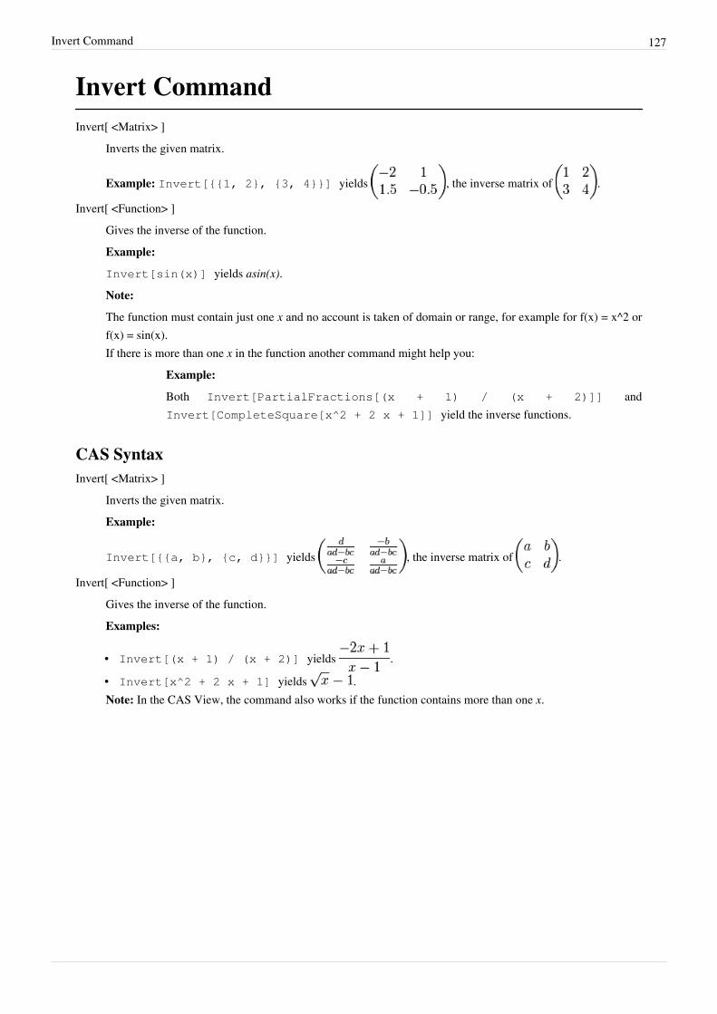
Invert Command 127

Invert CommandInvert[ <Matrix> ]

Inverts the given matrix.

Example: Invert[{{1, 2}, {3, 4}}] yields , the inverse matrix of .

Invert[ <Function> ]Gives the inverse of the function.Example:

Invert[sin(x)] yields asin(x).Note:

The function must contain just one x and no account is taken of domain or range, for example for f(x) = x^2 orf(x) = sin(x).If there is more than one x in the function another command might help you:

Example:

Both Invert[PartialFractions[(x + 1) / (x + 2)]] andInvert[CompleteSquare[x^2 + 2 x + 1]] yield the inverse functions.

CAS SyntaxInvert[ <Matrix> ]

Inverts the given matrix.Example:

Invert[{{a, b}, {c, d}}] yields , the inverse matrix of .

Invert[ <Function> ]Gives the inverse of the function.Examples:

• Invert[(x + 1) / (x + 2)] yields .

• Invert[x^2 + 2 x + 1] yields .Note: In the CAS View, the command also works if the function contains more than one x.

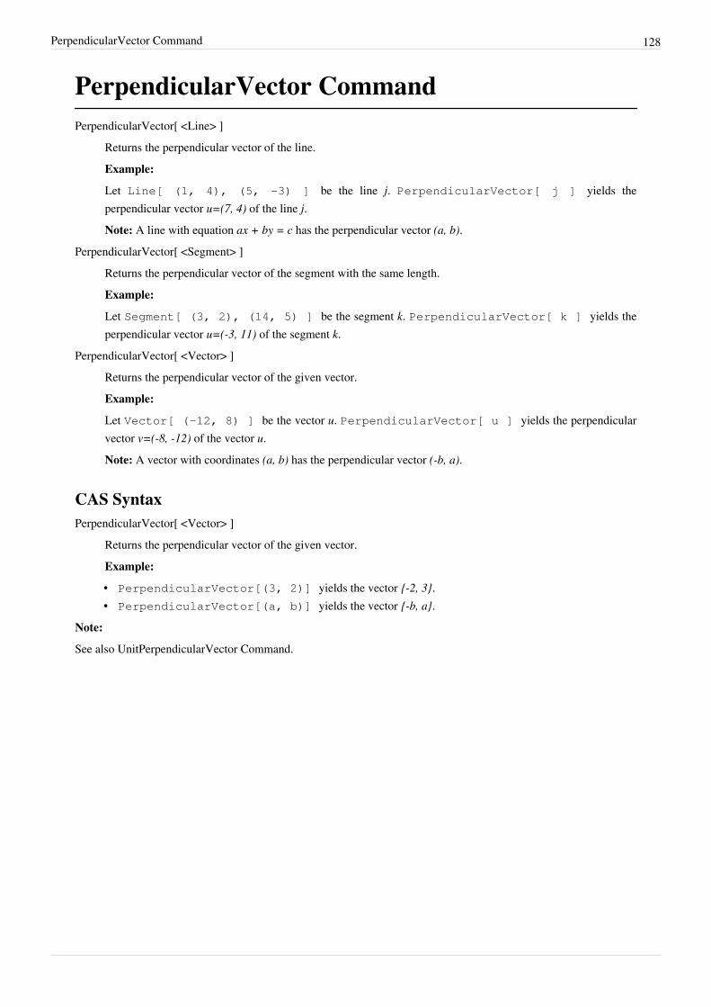
PerpendicularVector Command 128

PerpendicularVector CommandPerpendicularVector[ <Line> ]

Returns the perpendicular vector of the line.Example:

Let Line[ (1, 4), (5, -3) ] be the line j. PerpendicularVector[ j ] yields theperpendicular vector u=(7, 4) of the line j.Note: A line with equation ax + by = c has the perpendicular vector (a, b).

PerpendicularVector[ <Segment> ]Returns the perpendicular vector of the segment with the same length.Example:

Let Segment[ (3, 2), (14, 5) ] be the segment k. PerpendicularVector[ k ] yields theperpendicular vector u=(-3, 11) of the segment k.

PerpendicularVector[ <Vector> ]Returns the perpendicular vector of the given vector.Example:

Let Vector[ (-12, 8) ] be the vector u. PerpendicularVector[ u ] yields the perpendicularvector v=(-8, -12) of the vector u.Note: A vector with coordinates (a, b) has the perpendicular vector (-b, a).

CAS SyntaxPerpendicularVector[ <Vector> ]

Returns the perpendicular vector of the given vector.Example:

• PerpendicularVector[(3, 2)] yields the vector {-2, 3}.• PerpendicularVector[(a, b)] yields the vector {-b, a}.

Note:

See also UnitPerpendicularVector Command.

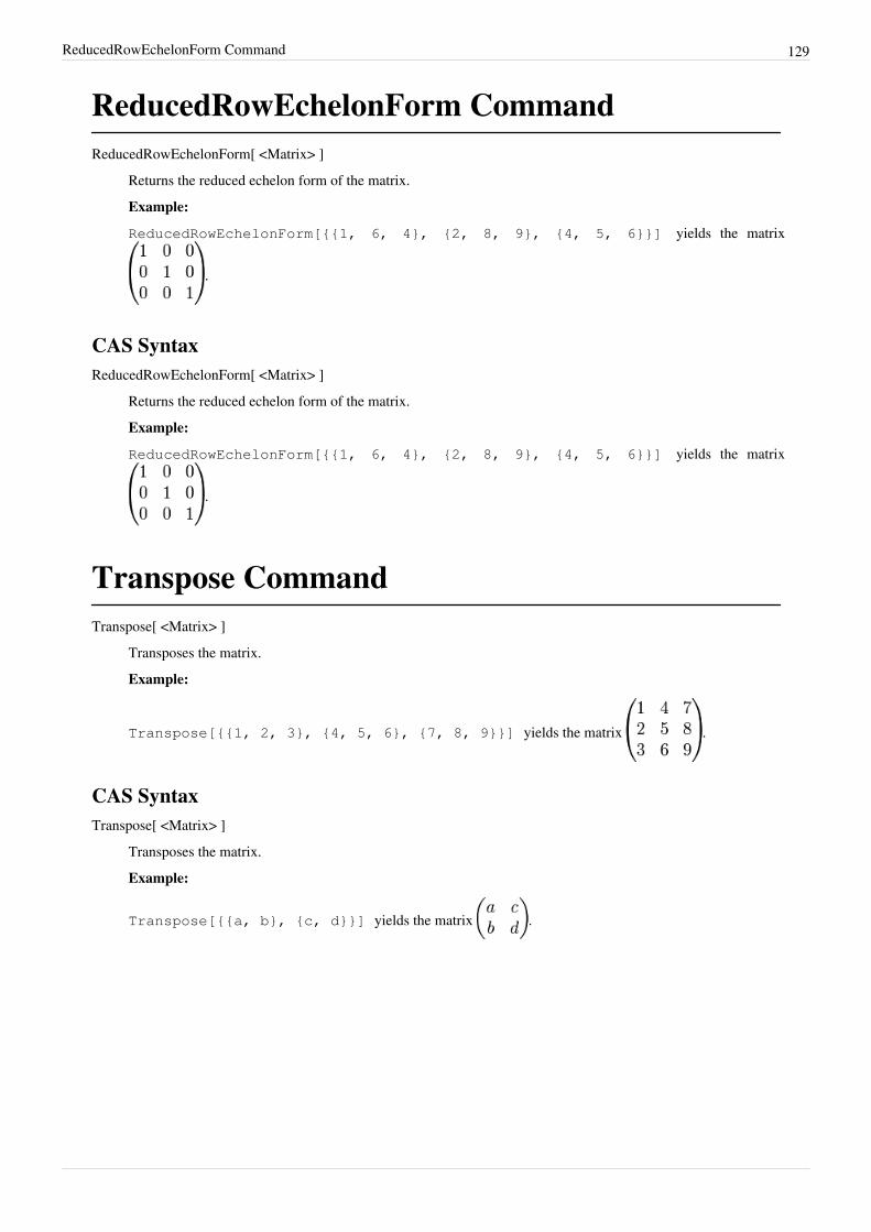
ReducedRowEchelonForm Command 129

ReducedRowEchelonForm CommandReducedRowEchelonForm[ <Matrix> ]

Returns the reduced echelon form of the matrix.Example:

ReducedRowEchelonForm[{{1, 6, 4}, {2, 8, 9}, {4, 5, 6}}] yields the matrix

.

CAS SyntaxReducedRowEchelonForm[ <Matrix> ]

Returns the reduced echelon form of the matrix.Example:

ReducedRowEchelonForm[{{1, 6, 4}, {2, 8, 9}, {4, 5, 6}}] yields the matrix

.

Transpose CommandTranspose[ <Matrix> ]

Transposes the matrix.Example:

Transpose[{{1, 2, 3}, {4, 5, 6}, {7, 8, 9}}] yields the matrix .

CAS SyntaxTranspose[ <Matrix> ]

Transposes the matrix.Example:

Transpose[{{a, b}, {c, d}}] yields the matrix .

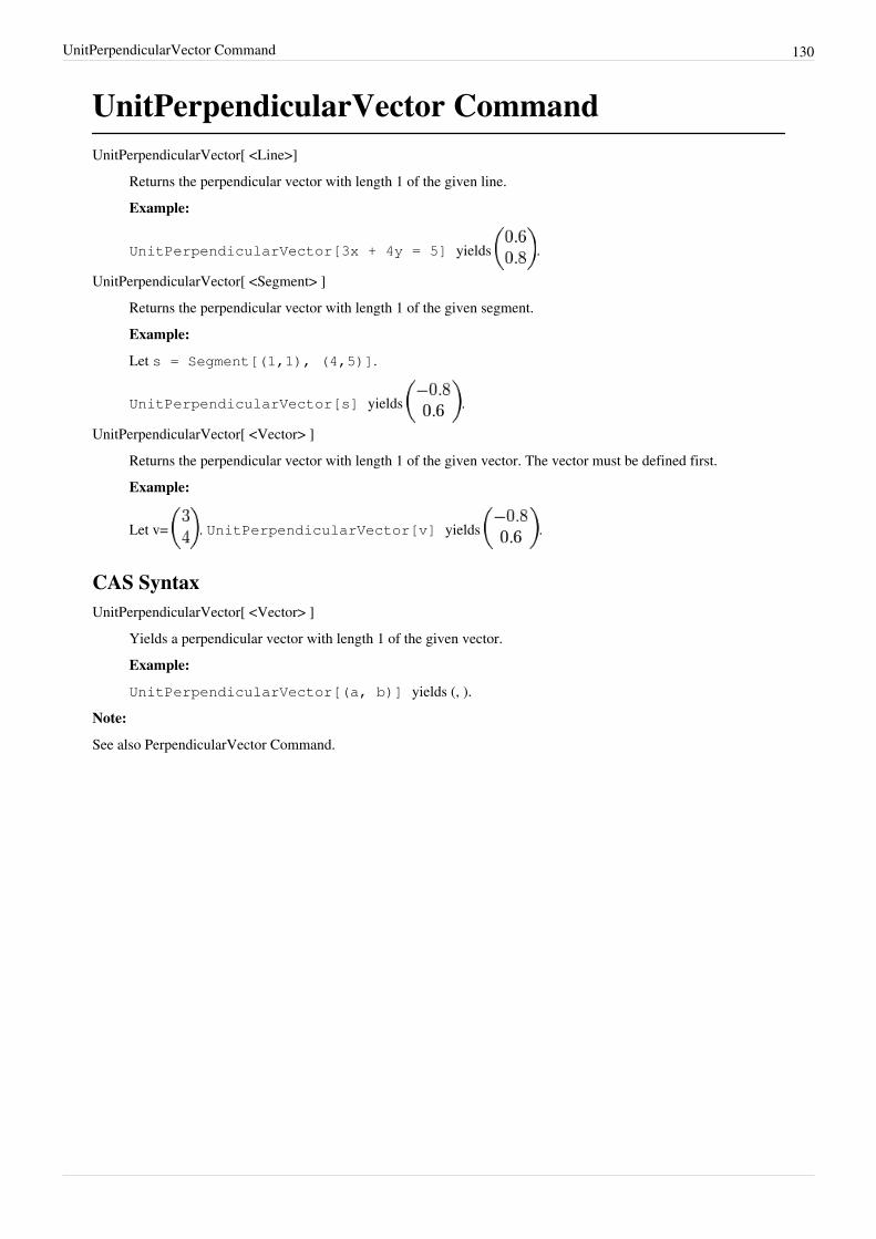
UnitPerpendicularVector Command 130

UnitPerpendicularVector CommandUnitPerpendicularVector[ <Line>]

Returns the perpendicular vector with length 1 of the given line.Example:

UnitPerpendicularVector[3x + 4y = 5] yields .

UnitPerpendicularVector[ <Segment> ]Returns the perpendicular vector with length 1 of the given segment.Example:

Let s = Segment[(1,1), (4,5)].

UnitPerpendicularVector[s] yields .

UnitPerpendicularVector[ <Vector> ]Returns the perpendicular vector with length 1 of the given vector. The vector must be defined first.Example:

Let v= . UnitPerpendicularVector[v] yields .

CAS SyntaxUnitPerpendicularVector[ <Vector> ]

Yields a perpendicular vector with length 1 of the given vector.Example:

UnitPerpendicularVector[(a, b)] yields (, ).Note:

See also PerpendicularVector Command.

UnitVector Command 131

UnitVector CommandUnitVector[ <Vector> ]

Yields a vector with length 1, which has the same direction and orientation as the given vector. The vectormust be defined first.Example:

Let v= . UnitVector[v] yields .

UnitVector[ <Line> ]Yields the direction vector of the given line with length 1.Example:

UnitVector[3x + 4y = 5] yields .

UnitVector[ <Segment> ]Yields the direction vector of the given segment with length 1.Example:

Let s = Segment[(1,1),(4,5)].

UnitVector[s] yields .

CAS SyntaxUnitVector[ <Vector> ]

Yields a vector with length 1, which has the same direction and orientation as the given vector.Example:

UnitVector[(a, b)] yields (, ).Example:

UnitVector[(2, 4, 4)] yields ( , , ).

Vector Command 132

Vector CommandVector[ <Start Point>, <End Point> ]

Creates a vector from Start Point to End Point.Example:

Vector[(1, 1), (3, 4)] yields u = .

Vector[ <Point> ]Returns the position vector of the given point.Example:

Vector[(3, 2)] yields u = .

Note: See also Vector tool.

Transformation Commands•• Dilate (Enlarge)•• Reflect•• Rotate•• Shear•• Stretch•• TranslateSee also Transformation tools

Dilate Command 133

Dilate CommandDilate[ <Object>, <Dilation Factor> ]

Dilates the object from a point of origin using the given factor.Dilate[ <Object>, <Dilation Factor>, <Dilation Center Point> ]

Dilates the object from a point, which is the dilation center point, using the given factor.Note: When dilating polygons, GeoGebra creates also all the transformed vertices and segments.

Note: See also Dilate from Point by Factor tool.

Reflect CommandReflect[ <Object>, <Point> ]

Reflects the geometric object through a given point.Note: When reflecting polygons through a point, the transformed vertices and segments are created as well.

Reflect[ <Object>, <Line> ]Reflects an object (e.g. an image) across a given line.Note: When reflecting polygons across a line, the transformed vertices and segments are created as well.

Reflect[ <Object>, <Circle> ]Inverts the geometric object with respect to a circle.

Note: See also Reflect about Point, Reflect about Line , and Reflect about Circle tools.

Rotate Command 134

Rotate CommandRotate[ <Object>, <Angle> ]

Rotates the geometric object by the angle around the axis origin.Rotate[ <Object>, <Angle>, <Point> ]

Rotates the geometric object by the angle around the given point.Note:Vectors are not rotated around axis origin, but around their initial point. When a polygon, segment or arc arerotated, also images of the vertices / endpoints and sides (in case of polygon) are created. This command also rotatesimages. For text rotation use RotateText Command. See also Rotate around Point ToolRotate around Point tool.

Shear CommandShear[ <Object>, <Line>, <Ratio> ]

Shears the object so that•• points on the line stay fixed.• points at distance d from the line are shifted by d ratio in direction of the line (direction of the shift is different

for halfplanes with respect to the line).A sheared plane figure maintains its original area.

Stretch CommandStretch[ <Object>, <Vector> ]

The object is stretched parallel to the given vector by the ratio given by the magnitude of the vector (i.e.points on the line perpendicular to the vector (through its startpoint) stay on their place and distance of otherpoints from the line is multiplied by given ratio.)

Stretch[ <Object>, <Line>, <Ratio> ]The object is stretched perpendicular to the line by the given ratio (i.e. points on the line aren't moved and thedistance of other points from the line is multiplied by given ratio.)

Translate Command 135

Translate CommandTranslate[ <Object>, <Vector> ]

Translates the geometric object by the vector.Note: When translating a polygon, the transformed new vertices and segments are created as well.

Translate[ <Vector>, <Start Point> ]Translates the vector to the start point.

Note: See also Translate by Vector tool.

Chart Commands•• BarChart•• BoxPlot•• DotPlot•• FrequencyPolygon•• Histogram•• HistogramRight•• NormalQuantilePlot•• ResidualPlot•• StemPlot

BarChart CommandBarChart[ <List of Data>, <List of Frequencies> ]

Creates a bar chart using the list of data with corresponding frequencies.Note: The numbers in the list of raw data need to be arranged in increasing order.Example:

•• BarChart[{10, 11, 12, 13, 14}, {5, 8, 12, 0, 1}]

•• BarChart[{5, 6, 7, 8, 9}, {1, 0, 12, 43, 3}]

•• BarChart[{0.3, 0.4, 0.5, 0.6}, {12, 33, 13, 4}]

BarChart[ <List of Raw Data>, <Width of Bars>]Creates a bar chart using the given raw data; the bars have the given width.Example: BarChart[ {1, 1, 1, 2, 2, 2, 2, 2, 3, 3, 3, 5, 5, 5, 5}, 1]

BarChart[ <List of Data> , <List of Frequencies>, <Width of Bars> ]Creates a bar chart using the list of data and corresponding frequencies; the bars have width w.Example:

• BarChart[{10, 11, 12, 13, 14}, {5, 8, 12, 0, 1}, 0.5] leaves gaps between bars.• BarChart[{10, 11, 12, 13, 14}, {5, 8, 12, 0, 1}, 0] produces a line graph.

BarChart[ <Start Value>, <End Value>, <List of Heights> ]Creates a bar chart over the given interval: the number of bars is determined by the length of the list, whoseelements are the heights of the bars.

BarChart Command 136

Example: BarChart[10, 20, {1, 2, 3, 4, 5} ] gives you a bar chart with five bars of specifiedheight in the interval [10, 20].

BarChart[ <Start Value>, <End Value> , <Expression>, <Variable>, <From Number>, <To Number> ]Creates a bar chart over the given interval [Start Value, End Value], that calculates the bars’ heights using theexpression whose variable k varies from number c to number d.Example: If p = 0.1, q = 0.9, and n = 10 are numbers, then BarChart[ -0.5, n + 0.5,BinomialCoefficient[n,k] * p^k * q^(n-k), k, 0, n ] gives you a bar chart in theinterval [-0.5, n+0.5]. The heights of the bars depend on the probabilities calculated using the givenexpression.

BarChart[ <Start Value>, <End Value>, <Expression>, <Variable>, <From Number>, <To Number>, <Step Width>]

Creates a bar chart over the given interval [Start Value, End Value], the bars’ heights are calculated using thegiven expression in which the variable k varies from number c to number d using step width s.

BoxPlot CommandBoxPlot[yOffset, yScale, List of Raw Data]

Creates a box plot using the given raw data and whose vertical position in the coordinate system is controlledby variable yOffset and whose height is influenced by factor yScale.Example: BoxPlot[0, 1, {2, 2, 3, 4, 5, 5, 6, 7, 7, 8, 8, 8, 9}]

BoxPlot[yOffset, yScale, Start Value, Q1, Median, Q3, End Value]Creates a box plot for the given statistical data in interval [Start Value, End Value].

BoxPlot[ <yOffset>, <yScale>, <List of Raw Data>, <Boolean Outliers> ]This allows outliers to be plotted as "X"s rather than included in the boxplot. For this command, outliers aredata lying below Q1 - 1.5 * IQR or above Q3 + 1.5 * IQR.

BoxPlot[ <yOffset>, <yScale>, <List of Data>, <List of Frequencies>, <Boolean Outliers> ]This allows data from a frequency table to be easily plotted as a boxplot.

DotPlot Command 137

DotPlot CommandDotPlot[ <List of Raw Data> ]

Returns a dot plot for the given list of numbers, as well as the list of the dot plot points. If a number n appearsin the list of raw data k times, the returned list contains points (n, 1), (n, 2), ..., (n, k).Example:

DotPlot[{2, 5, 3, 4, 3, 5, 3}] yields {(2, 1), (3, 1), (3, 2), (3, 3), (4, 1), (5, 1), (5, 2)}.

FrequencyPolygon CommandNote: Frequency polygon is a line graph drawn by joining all the midpoints of the top of the bars of a histogram.Therefore usage of this command is the same as usage of Histogram Command.FrequencyPolygon[ <List of Class Boundaries>, <List of Heights> ]

Creates a frequency polygon with vertices in given heights. The class boundaries determine the x-coordinateof each vertex.

FrequencyPolygon[ <List of Class Boundaries>, <List of Raw Data>, <Boolean Use Density>, <Density ScaleFactor (optional)> ]

Creates a frequency polygon using the raw data. The class boundaries determine the x-coordinates of verticesand are used to determine how many data elements lie in each class. The y-coordinate of a vertex isdetermined as follows

• If Use Density = true, height = (Density Scale Factor) * (class frequency) / (class width)• If Use Density = false, height = class frequency

By default, Use Density = true and Density Scale Factor = 1.FrequencyPolygon[ <Boolean Cumulative>, <List of Class Boundaries>, <List of Raw Data>, <Boolean UseDensity> , <Density Scale Factor (optional)> ]

If Cumulative is true this creates a frequency polygon where each vertex y-coordinate equals the frequency ofthe class plus the sum of all previous frequencies.

Note: For examples see Histogram Command.

Histogram Command 138

Histogram CommandHistogram[ <List of Class Boundaries>, <List of Heights> ]

Creates a histogram with bars of the given heights. The class boundaries determine the width and position ofeach bar of the histogram.

Example: Histogram[{0, 1, 2, 3, 4, 5}, {2, 6, 8, 3, 1}] creates a histogram with 5 bars ofthe given heights. The first bar is positioned at the interval [0, 1], the second bar is positioned at the interval [1, 2],and so on.Histogram[ <List of Class Boundaries>, <List of Raw Data>, <Boolean Use Density>, <Density ScaleFactor>(optional) ]

Creates a histogram using the raw data. The class boundaries determine the width and position of each bar ofthe histogram and are used to determine how many data elements lie in each class. Bar height is determined asfollows

• If Use Density = true, height = (Density Scale Factor) * (class frequency) / (class width)• If Use Density = false, height = class frequency

By default, Use Density = true and Density Scale Factor = 1. This creates a histogram with total area = n, thenumber of data values.

Note: All elements of Raw Data must be within the interval of the class boundaries or the histogram will return“undefined”.Note: By convention this uses the a ≤ x < b rule for each class except for the last class which is a ≤ x ≤ bExample: (Default Histogram)Histogram[{10, 20, 30, 40}, {10, 11, 11, 12, 18, 20, 25, 40}, true] creates a histogramwith 3 bars, with the heights 0.5 (first bar), 0.2 (second bar), and 0.1 (third bar). This histogram has total area =0.5*10 + 0.2*10 + 0.1*10 = 8.Example: (Count Histogram)Histogram[{10, 20, 30, 40}, {10, 11, 11, 12, 18, 20, 25, 40}, false] creates a histogramwith 3 bars, with the heights 5 (first bar), 2 (second bar), and 1 (third bar). This histogram does not use densityscaling and gives bar heights that equal the count of values in each class.Example: (Relative Frequency Histogram)Histogram[{10, 20, 30, 40}, {10, 11, 11, 12, 18, 20, 25, 40}, true, 10/ 8]creates a histogram with 3 bars, with the heights 0.625 (first bar), 0.25 (second bar), and 0.125 (third bar). Thishistogram uses density scaling to give bar heights that equal the proportion of values in each class. If n is the numberof data values, and the classes have constant width w, then Density Scale Factor = w/n creates a relative histogram.Example: (Normalized Histogram)Histogram[{10, 20, 30, 40}, {10, 11, 11, 12, 18, 20, 25, 40}, true, 1/8] creates ahistogram with 3 bars, with the heights .0625 (first bar), .025 (second bar), and .0125 (third bar). This histogram hastotal area = .0625*10 + .025*10 + .0125*10 = 1. If n is the number of data values, then Density Scale Factor = 1/ncreates a normalized histogram with total area = 1. This is useful for fitting a histogram with a density curve.Histogram[ <Boolean Cumulative>, <List of Class Boundaries>, <List of Raw Data>, <Boolean Use Density> ,<Density Scale Factor> (optional) ]

If Cumulative is true this creates a histogram where each bar height equals the frequency of the class plus thesum of all previous frequencies.

Example: :Histogram[true, {10, 20, 30, 40}, {10, 11, 11, 12, 18, 20, 25, 40},true] creates a histogram with 3 bars, with the heights 0.5 (first bar), 0.7 (second bar), and 0.8 (third bar).

HistogramRight Command 139

HistogramRight CommandHistogramRight[ <List of Class Boundaries>, <List of Heights> ]

Same as Histogram[<List of Class Boundaries>, <List of Heights>]HistogramRight[ <List of Class Boundaries>, <List of Raw Data>, <Boolean Use Density> , <Density Scale Factor>(optional) ]

Same as Histogram[<List of Class Boundaries>, <List of Raw Data>, <BooleanUse Density>, <Density Scale Factor>], except that if a datum is equal to the right border of aclass, it is counted in this class and not in the next one.

HistogramRight[ <Boolean Cumulative>, <List of Class Boundaries>, <List of Raw Data>, <Boolean Use Density>, <Density Scale Factor> (optional) ]

Same as Histogram[<Boolean Cumulative>, <List of Class Boundaries>, <Listof Raw Data>, <Boolean Use Density>, <Density Scale Factor>], except that if adatum is equal to the right border of a class, it is counted in this class and not in the next one.

Note: By convention this uses the a < x ≤ b rule for each class except for the first class which is a ≤ x ≤ b

NormalQuantilePlot CommandNormalQuantilePlot[ <List of Raw Data> ]

Creates a normal quantile plot from the given list of data and draws a line through the points showing the idealplot for exactly normal data. Points are formed by plotting data values on the x axis against their expectednormal score (Z-score) on the y axis.

ResidualPlot Command 140

ResidualPlot CommandResidualPlot[ <List of Points>, <Function> ]

Returns a list of points whose x-coordinates are equal to the x-coordinates of the elements of the given list, andy-coordinates are the residuals with respect to f.If the i-th element of the given list is a point (a,b) then i-th element of the result is (a,b-f(a)).Example:

Let list = {(-1, 1), (-0.51, 2), (0, 0.61), (0.51, -1.41), (0.54, 1.97),(1.11, 0.42), (1.21, 2.53), (-0.8, -0.12)} be the list of points and f(x) = x^5 +x^4 - x - 1 the function. The ResidualPlot[ list, f ] command yields list1 = {(-1, 1), (-0.51,2.46), (0, 1.61), (0.51, 0), (0.54, 3.38), (1.11, -0.66), (1.21, 0), (-0.8, 0)} and creates the corresponding pointsin Graphics view.

StemPlot CommandStemPlot[ <List> ]

Returns a stem plot of the given list of numbers. Outliers are removed from the plot and listed separately.An outlier is defined as a value outside the interval [ Q1 - 1.5 (Q3 - Q1) , Q3 + 1.5 (Q3 - Q1) ].

StemPlot[ <List>, <Adjustment -1|0|1> ]Returns a stem plot of the given list of numbers.If Adjustment = -1 the default stem unit is divided by 10If Adjustment = 0 nothing is changedIf Adjustment = 1 the default stem unit is multiplied by 10

Statistics Commands 141

Statistics Commands•• ANOVA•• Classes•• CorrelationCoefficient•• Covariance•• Fit•• FitExp•• FitGrowth•• FitLine•• FitLineX•• FitLog•• FitLogistic•• FitPoly•• FitPow•• FitSin•• Frequency•• FrequencyTable•• GeometricMean•• HarmonicMean•• Mean•• MeanX•• MeanY•• Median•• Mode•• Percentile•• Q1•• Q3•• RootMeanSquare•• RSquare•• Sample•• SampleSD•• SampleSDX•• SampleSDY•• SampleVariance•• SD•• SDX•• SDY•• Shuffle•• SigmaXX•• SigmaXY•• SigmaYY•• Spearman•• Sum•• SumSquaredErrors•• Sxx•• Sxy

Statistics Commands 142

•• Syy•• TMeanEstimate•• TMean2Estimate•• TTest•• TTest2•• TTestPaired•• VarianceSee also Probability Calculator.

ANOVA CommandANOVA[ <List>, <List>, ...]

Performs a one-way ANOVA test on the given lists of numbers.Results are returned in list form as {P value, F test statistic}.

Classes CommandClasses[ <List of Data>, <Start>, <Width of Classes> ]

Gives a list of class boundaries. The first boundary (min) is equal to Start, the last boundary (max) will be atleast the maximum of the List and the boundaries will be equally spaced between min and max.Example: Classes[{0.1, 0.2, 0.4, 1.1}, 0, 1] gives {0, 1, 2}

Classes[ <List of Data>, <Number of Classes> ]Gives a list of class boundaries. The first boundary (min) is equal to the minimum of the List, the lastboundary (max) will be the maximum of the List and the boundaries will be equally spaced between min andmax.Example: Classes[{1, 3, 5, 7, 8, 9, 10}, 3] gives {1, 4, 7, 10}

Note: By convention this uses the a ≤ x < b rule for each class except for the last class which is a ≤ x ≤ b

Covariance Command 143

Covariance CommandCovariance[ <List of Numbers>, <List of Numbers> ]

Calculates the covariance between the elements of the specified lists.Example:

Covariance[{1, 2, 3}, {1, 3, 7}] yields 2, the covariance of {1, 2, 3} and {1, 3, 7}.Covariance[ <List of Points> ]

Calculates the covariance between the x and y coordinates of the specified points.Example:

Covariance[{(1, 1), (2, 3), (3, 7)}] yields 2, the covariance of {1, 2, 3} and {1, 3, 7}.

CAS SyntaxCovariance[ <List of Numbers>, <List of Numbers> ]

Calculates the covariance between the elements of the specified lists.Example:

Covariance[{1, 2, 3}, {1, 3, 7}] yields 2, the covariance of {1, 2, 3} and {1, 3, 7}.Covariance[ <List of Points> ]

Calculates the covariance between the x and y coordinates of the specified points.Example:

Covariance[{(1, 1), (2, 3), (3, 7)}] yields 2, the covariance of {1, 2, 3} and {1, 3, 7}.

Fit Command 144

Fit CommandFit[ <List of Points>, <List of Functions> ]

Calculates a linear combination of the functions that best fit the points in the list.Example:

• Fit[{(-2, 3), (0, 1), (2, 1), (2, 3)}, {x^2, x}] yields 0.625 x^2 - 0.25x.• Let L = {A, B, C, ...}, f(x) = 1, g(x) = x, h(x) = e^x, F = {f, g, h}.Fit[L, F] calculates a function of the form a + b x + c e^x that fits the points in the list.

Fit[ <List of points>, <Function> ]Calculates a minimum squared error function to the points in the list. The function must depend on one ormore sliders, that are taken as start values of parameters to be optimized. The non-linear iteration might notconverge, but adjusting the sliders to a better starting point might help.Example:

Let a be slider with interval from -5 to 5 and increment 1.Fit[{(-2, 3), (0, 1), (2, 1), (2, 3)}, a + x^2] yields -1 + x^2.

Note: Other point fitting commands are FitExp, FitGrowth, FitLine, FitLineX, FitLog, FitLogistic, FitPoly, FitPowand FitSin.

FitExp CommandFitExp[ <List of Points> ]

Calculates the exponential regression curve in the form aℯbx.Example:

FitExp[{(0, 1), (2, 4)}] yields ℯ0.69x.

CAS SyntaxFitExp[ <List of Points> ]

Calculates the exponential regression curve.Example:

FitExp[{(0, 1), (2, 4)}] yields ℯ0.69x.Note:

• If you want the answer in the form then use the FitGrowth Command.• Euler's number ℯ can be obtained by pressing ALT + e.• See also Fit, FitGrowth, FitLine, FitLineX, FitLog, FitLogistic, FitPoly, FitPow and FitSin.

FitGrowth Command 145

FitGrowth CommandFitGrowth[ <List of Points> ]

Calculates a function of the form to the points in the list. (Just like FitExp[ <List of Points> ], for userswho do not know the meaning of exponential growth).Example:

FitGrowth[{(0, 1), (2, 3), (4, 3), (6, 4)}] yields 1.31 1.23x.

CAS SyntaxFitGrowth[ <List of Points> ]

Calculates a function of the form to the points in the list.Example:

FitGrowth[{(0, 1), (2, 3), (4, 3), (6, 4)}] yields 1.31 1.23x.Note: See also Fit, FitExp, FitLine, FitLineX, FitLog, FitLogistic, FitPoly, FitPow and FitSin.

FitLineX CommandFitLineX[ <List of Points> ]

Calculates the x on y regression line of the points.Example:

FitLineX[{(-1, 3), (2, 1), (3, 4), (5, 3), (6, 5)}] yields 1.1x - 0.1.

CAS SyntaxFitLineX[ <List of Points> ]

Calculates the x on y regression line of the points.Example:

FitLineX[{(-1, 3), (2, 1), (3, 4), (5, 3), (6, 5)}] yields 1.1x - 0.1.

Note: See also Best Fit Line tool and FitLine Command.

FitLine Command 146

FitLine CommandFitLine[ <List of Points> ]

Calculates the y on x regression line of the points.Example:

FitLine[{(-2, 1), (1, 2), (2, 4), (4, 3), (5, 4)}] yields 0.4x + 2.

CAS SyntaxFitLine[ <List of Points> ]

Calculates the y on x regression line of the points.Example:

FitLine[{(-2, 1), (1, 2), (2, 4), (4, 3), (5, 4)}] yields 0.4x + 2.

Note: See also Best Fit Line tool and FitLineX Command.

FitLog CommandFitLog[ <List of Points> ]

Calculates the logarithmic regression curve.Example:

FitLog[{(ℯ, 1), (ℯ^2, 4)}] yields -2 + 3 ln(x).

CAS SyntaxFitLog[ <List of Points> ]

Calculates the logarithmic regression curve.Example:

FitLog[{(ℯ, 1), (ℯ^2, 4)}] yields 3 ln(x) - 2.Note:

• Euler's number ℯ can be obtained by pressing ALT + e.• See also FitExp Command, FitPoly Command, FitPow Command and FitSin Command.

FitLogistic Command 147

FitLogistic CommandFitLogistic[ <List of Points> ]

Calculates the regression curve in the form a/(1 + b e^(-kx)).Example:

FitLogistic[{(-6, 2), (0, 2), (3, 4), (3.4, 8)}] yields .

CAS SyntaxFitLogistic[ <List of Points> ]

Calculates the regression curve in the form a/(1 + b e^(-kx)).Example:

FitLogistic[{(-6, 2), (0, 2), (3, 4), (3.4, 8)}] yields .

Note:

•• The first and last data points should be fairly close to the curve. The list should have at least 3 points, preferablymore.

• See also Fit, FitExp, FitGrowth, FitLine, FitLineX, FitLog, FitPoly, FitPow and FitSin.

FitPoly CommandFitPoly[ <List of Points>, <Degree of Polynomial> ]

Calculates the regression polynomial of degree n.Example:

FitPoly[{(-1, -1), (0, 1), (1, 1), (2, 5)}, 3] yields f(x) = x3 - x2 + 1.

CAS SyntaxFitPoly[ <List of Points>, <Degree of Polynomial> ]

Calculates the regression polynomial of degree n.Example:

FitPoly[{(-1, -1), (0, 1), (1, 1), (2, 5)}, 3] yields x3 - x2 + 1.Note:

• For order n there must be at least n + 1 Points in the list.• See also FitExp Command, FitLog Command, FitPow Command and FitSin Command.

FitPow Command 148

FitPow CommandFitPow[ <List of Points> ]

Calculates the regression curve in the form a x^b.Example:

FitPow[{(1, 1), (3, 2), (7, 4)}] creates the regression curve f(x) = 0.97 x^{0.71}.

CAS SyntaxFitPow[ <List of Points> ]

Calculates the regression curve in the form a x^b.Example:

FitPow[{(1, 1), (3, 2), (7, 4)}] yields 0.97 x^{0.71}.Note:

•• All points used need to be in the first quadrant of the coordinate system.• See also FitExp Command, FitLog Command, FitPoly Command, and FitSin Command.

FitSin CommandFitSin[ <List of Points> ]

Calculates the regression curve in the form a + b sin (c x + d).Example:

FitSin[{(1, 1), (2, 2), (3, 1), (4, 0), (5, 1), (6, 2)}] yields f(x) = 1 + 1 sin(1.5708 x - 1.5708).

CAS SyntaxFitSin[ <List of Points> ]

Calculates the regression curve in the form a + b sin (c x + d).Example:

FitSin[{(1, 1), (2, 2), (3, 1), (4, 0), (5, 1), (6, 2)}] yields 1 + 1 sin (1.5708 x- 1.5708).

Note:

•• The list should have at least four points, preferably more. The list should cover at least two extremal points. Thefirst two local extremal points should not be too different from the absolute extremal points of the curve.

• See also FitExp Command, FitLog Command, FitPoly Command and FitPow Command.

Frequency Command 149

Frequency CommandFrequency[ <List of Raw Data> ]

Returns a list with a count of the occurrences of each unique value in the given list of data. This input list canbe numbers or text. The list is sorted in ascending order of the unique values. To get a list of the correspondingunique values use the Unique Command.Example: Enter list1 = { "a", "a", "x", "x", "x", "b" }. Frequency[list1] returnsthe list { 2, 1, 3 }. Unique[list1] returns the list { "a", "b", "x" }.

Frequency[ <Boolean Cumulative>, <List of Raw Data> ]If Cumulative = false, returns the same list as Frequency[ <List of Raw Data> ]If Cumulative = true, returns a list of cumulative frequencies for Frequency[ <List of Raw Data> ] .Example: Enter list1 = { 0, 0, 0, 1, 1, 2 }. Frequency[true, list1] returns the list {3, 5, 6 }. Frequency[false, list1] returns the list { 3, 2, 1}. Unique[list1] returns the list { 0,1, 2 }.

Frequency[ <List of Class Boundaries>, <List of Raw Data> ]Returns a list of the counts of values from the given data list that lie within intervals of the form [a, b), where aand b are all the couples of consecutive numbers in the given class boundaries list. The highest interval has theform [a, b].Example: Frequency[{1, 2, 3}, {1, 1, 2, 3}] returns the list { 2, 2 }.

Frequency[ <Boolean Cumulative>, <List of Class Boundaries>,<List of Raw Data> ]If Cumulative = false, returns the same list as Frequency[ <List of Class Boundaries>, <List of Raw Data> ]If Cumulative = true, returns a list of cumulative frequencies for Frequency[ <List of Class Boundaries>, <Listof Raw Data> ]

Frequency[ <List of Class Boundaries>, <List of Raw Data>, <Use Density> , <Density Scale Factor> (optional) ]Returns a list of frequencies for the corresponding Histogram Command.If Use density = false, returns the same list as Frequency[ <List of Class Boundaries>, <List of Raw Data> ]If Use density = true, returns the list of frequencies of each class.Example: Let data = {1, 2, 2, 2, 3, 3, 4, 4, 4, 4} be the list of raw data andclasses={0, 2, 5} the list of class boundaries. Then Frequency[classes, data, false]and Frequency[classes, data] both return the list {1, 9}, while Frequency[classes, data,true] returns the list {0.5, 3}.

Frequency[ <Boolean Cumulative>, <List of Class Boundaries>, <List of Raw Data>, <Use Density> , <DensityScale Factor> (optional) ]

Returns a list of frequencies for the corresponding Histogram Command.Frequency[ <List of Text>, <List of Text> ]

Returns a contingency matrix containing counts of paired values from the two lists. The rows of the matrixcorrespond to the unique values in the first list, and the columns correspond to the unique values in the secondlist. To get a list of the unique values for each list use the command Unique Command.Example: Let list1 = {"a", "b", "b", "c", "c", "c", "c"} and list2 = {"a", "b", "a", "a", "c", "c", "d"}. Then Frequency[ list1, list2 ] returns the matrix

Frequency Command 150

Note: See also the ContingencyTable command.

FrequencyTable CommandFrequencyTable[ <List of Raw Data> ]

Returns a table (as text) whose first column contains sorted list of unique elements of list L and second columncontains the count of the occurrences of value in the first column. List L can be numbers or text.

FrequencyTable[ <Boolean Cumulative>, <List of Raw Data> ]If Cumulative = false, returns the same table as Frequency[ <List of Raw Data> ]If Cumulative = true, returns a table whose first column is the same as in FrequencyTable[ <List of RawData> ] and the second contains cumulative frequencies of values in the first column.

FrequencyTable[ <List of Class Boundaries>, <List of Raw Data> ]Returns a table (as text) whose first column contains intervals (classes) and second column contains the countof numbers in List of Raw Data, which belong to the interval in the first column. All intervals except thehighest interval are of the form [a, b). The highest interval has the form [a, b].

FrequencyTable[ <Boolean Cumulative>, <List of Class Boundaries>, <List of Raw Data> ]If Cumulative = false, returns the same table as FrequencyTable[ <List of Class Boundaries>, <List of RawData> ]If Cumulative = true, returns a table whose first column is the same as in FrequencyTable[ <List of RawData> ] and the second contains cumulative frequencies of values in the first column.

FrequencyTable[ <List of Class Boundaries>, <List of Raw Data>, <Use Density> , <Density Scale Factor(optional)> ]

Returns a table (as text) whose first column contains intervals (classes) and second contains frequencies for thecorresponding Histogram Command.

FrequencyTable[ <Boolean Cumulative>, <List of Class Boundaries>, <List of Raw Data>, <Use Density> ,<Density Scale Factor (optional)> ]

Returns a table (as text) whose first column contains intervals (classes) and second contains frequencies for thecorresponding Histogram Command.

Note: This command is similar to Frequency Command and Histogram Command. Articles about these commandscontain some related examples.

GeometricMean Command 151

GeometricMean CommandGeometricMean[List of Numbers]

Returns the geometric mean of given list of numbers.Example: GeometricMean[{13, 7, 26, 5, 19}] yields 11.76.

HarmonicMean CommandHarmonicMean[ <List of Numbers> ]

Returns the harmonic mean of given list of numbers.Example: HarmonicMean[{13, 7, 26, 5, 19}] yields 9.79.

Mean CommandMean[ <List of Raw Data> ]

Calculates the arithmetic mean of list elements.Example:

• Mean[{1, 2, 3, 2, 4, 1, 3, 2}] yields a = 2.25 and• Mean[{1, 3, 5, 9, 13}] yields a = 6.2.

Mean[ <List of Numbers>, <List of Frequencies> ]Calculates the weighted mean of the list elements.Example:

• Mean[{1, 2, 3, 4}, {6, 1, 3, 6}] yields a = 2.56 and• Mean[{1, 2, 3, 4}, {1, 1, 3, 6}] yields a = 3.27.

CAS SyntaxMean[ <List of Numbers> ]

Calculates the arithmetic mean of the list elements.Example:

Mean[{1, 2, 3, 5, 44}] yields a = 11.Note:

See also MeanX, MeanY, and SD commands.

MeanX Command 152

MeanX CommandMeanX[ <List of Points> ]

Calculates the mean of the x-coordinates of the points in the list.Example: MeanX[{(0,0), (3,2), (5,1), (2,1), (2,4)}] yields 2.4

MeanY CommandMeanY[ <List of Points> ]

Calculates the mean of the y-coordinates of the points in the list.Example: MeanY[{(0,0), (3,2), (5,1), (2,1), (2,4)}] yields 1.6

Median CommandMedian[ <List of Raw Data> ]

Determines the median of the list elements.Examples:

• Median[{1, 2, 3}] yields 2.• Median[{1, 1, 8, 8}] yields 4.5.

Median[ <List of Numbers>, <List of Frequencies> ]Calculates the weighted median of the list elements.Example:

• Median[{1, 2, 3}, {4, 1, 3}] yields 1.5.• Median[{1, 2, 3}, {4, 1, 6}] yields 3.

CAS SyntaxMedian[ <List of Numbers> ]

Determines the median of the list elements.Examples:

• Median[{1, 2, 3}] yields 2.• Median[{1, 1, 8, 8}] yields 4.5

Note:

•• If the length of the given list is even, the arithmetic mean of the two center elements is returned.• See also Mean command.

Mode Command 153

Mode CommandMode[ <List of Numbers> ]

Determines the mode(s) of the list elements.Examples:Mode[{1, 2, 3, 4}] returns an empty list {}.Mode[{1, 1, 1, 2, 3, 4}] returns the list {1} .Mode[{1, 1,2, 2, 3, 3, 4}] returns the list {1, 2, 3}.

CorrelationCoefficient CommandCorrelationCoefficient[ <List of x-coordinates>, <List of y-coordinates> ]

Calculates the product moment correlation coefficient using the given x- and y-coordinates.Example:

CorrelationCoefficient[{1, 3, 2, 1, 5, 2}, {1, 6, 4, 3, 3, 2}] yields 0.36.CorrelationCoefficient[ <List of Points> ]

Calculates the product moment correlation coefficient using the coordinates of the given points.Example:

CorrelationCoefficient[{(1, 1), (3, 6), (2, 4), (1, 3), (5, 3), (2, 2)}]

yields 0.36.

Percentile CommandPercentile[ <List of Numbers>, <Percent> ]

Let P equal the given Percent.Returns the value that cuts off the first P percent of the list of numbers, when the list is sorted in ascendingorder. Percent must be a number in the interval 0 < P ≤ 1.Example:

Percentile[{1, 2, 3, 4}, 0.25] yields 1.25.Note: The commands Quartile and Percentile use different rules and do not always return matchingresults.Example:Q1[{1, 2, 3, 4}] yields 1.5.Percentile[{1, 2, 3, 4}, 0.25] yields 1.25.

Q1 Command 154

Q1 CommandQ1[ <List of Raw Data> ]

Determines the lower quartile of the list elements.Example:

Q1[{1, 2, 3, 4}] yields 1.5.Q1[ <List of Numbers>, <List of Frequencies> ]

Determines the lower quartile of the list elements considering the frequencies.Example:

Q1[{1, 2, 3, 4}, {3, 2, 4, 2}] yields 1.Note:

GeoGebra uses the Moore & McCabe (2002) method to calculate quartiles, see http:/ / mathworld. wolfram. com/Quartile. html

Q3 CommandQ3[ <List of Raw Data> ]

Determines the upper quartile of the list elements.Example:

Q3[{1, 2, 3, 4}] yields 3.5.Q3[ <List of Numbers>, <List of Frequencies> ]

Determines the upper quartile of the list elements considering the frequencies.Example:

Q3[{1, 2, 3, 4}, {3, 2, 4, 2}] yields 3.Note:

GeoGebra uses the Moore & McCabe (2002) method to calculate quartiles, see http:/ / mathworld. wolfram. com/Quartile. html

RSquare Command 155

RSquare CommandRSquare[ <List of Points>, <Function> ]

Calculates the coefficient of determination R² = 1-SSE/Syy, between the y-values of the points in the list andthe function values of the x-values in the list.Example:

RSquare[{(-3, 2), (-2, 1), (-1, 3), (0, 4), (1, 2), (2, 4), (3, 3), (4,

5), (6, 4)}, 0.5x + 2.5] yields 0.28.

RootMeanSquare CommandRootMeanSquare[ <List of Numbers> ]

Returns the root mean square of given list of numbers.Example:

RootMeanSquare[{3, 4, 5, 3, 2, 3, 4}] yields 3.5456.

SD CommandSD[ <List of Numbers> ]

Calculates the standard deviation of the numbers in the list.Example: SD[{1, 2, 3, 4, 5}] yields 1.41

SD[ <List of Numbers>, <List of Frequencies> ]Calculates the weighted standard deviation of the given numbers.Example: SD[{20, 40, 41, 42, 40, 54}, {20, 6, 4, 5, 2} ] yields 5.96

CAS SyntaxSD[ <List of Numbers> ]

Calculates the standard deviation of the numbers in the list.Example:

• SD[{1, 2, 3, 4, 5}] yields .

• SD[{-3 + 2 x, -1- 4 x, -2 + 5 x^2}] is evaluated as $\frac{\sqrt{25x⁴ + 10x³ + 28x² -18x + 3} \; \sqrt{2} } { \; 3 \; }$.

Note:

See also Mean Command.

SDX Command 156

SDX CommandSDX[ <List of Points> ]

Returns standard deviation of x-coordinates of points from the given list.Example: SDX[{(1, 1), (2, 2), (3, 1), (3, 3), (4, 2), (3, -1)}] yields a = 0.97.

SDY CommandSDY[ <List of Points> ]

Returns standard deviation of y-coordinates of points from the given list.Example: SDY[{(1, 1), (2, 2), (3, 1), (3, 3), (4, 2), (3, -1)}] yields a = 1.25.

Sxx CommandSxx[ <List of Numbers> ]

Calculates the statistic .

Sxx[ <List of Points> ]

Calculates the statistic using the x-coordinates of the given points.

Sxy CommandSxy[ <List of Points> ]

Calculates the statistic using the coordinates of the given points.

Sxy[ <List of Numbers>, <List of Numbers> ]

Calculates the statistic , where x are the values in the first list, and y are the values in

the second given list.

Syy Command 157

Syy CommandSyy[ <List of Points> ]

Calculates the statistic using the y-coordinates of the given points.

Sample CommandSample[ <List>, <Size> ]

Returns list of n randomly chosen elements of a list; elements can be chosen several times.Example:

Sample[{1, 2, 3, 4, 5}, 5] yields for example list1 = {1, 2, 1, 5, 4}.Sample[ <List>, <Size>, <With Replacement> ]

Returns list of n randomly chosen elements of a list. Elements can be chosen several times if and only if thelast parameter is true.Example:

Sample[{1, 2, 3, 4, 5}, 5, true] yields for example list1 = {2, 3, 3, 4, 5}.

CAS SyntaxSample[ <List>, <Size> ]

Returns list of n randomly chosen elements of a list; elements can be chosen several times.Example:

Sample[{-5, 2, a, 7, c}, 3] yields for example {a, 7, -5}.Sample[ <List>, <Size>, <With Replacement> ]

Returns list of n randomly chosen elements of a list. Elements can be chosen several times if and only if thelast parameter is true.Example:

The list can include lists as well: Let List1 be {1, 2, 3}.Sample[{List1, 4, 5, 6, 7, 8}, 3, false] yields for example {6, {1, 2, 3}, 4}.

SampleSD Command 158

SampleSD CommandSampleSD[ <List of Numbers> ]

Returns sample standard deviation of given list of numbers.Example:

SampleSD[{1, 2, 3}] yields 1.SampleSD[ <List of Numbers>, <List of Frequencies> ]

Returns the standard deviation of the sample of numbers having the given frequencies.Example:

SampleSD[{1, 2, 3, 4, 4},{1, 1, 1, 2}] yields 1.08.

CAS SyntaxSampleSD[ <List of Numbers> ]

Returns sample standard deviation of given list of numbers. If the list contains undefined variables, it yields aformula for the sample standard deviation.Example:

SampleSD[{1, 2, a}] yields .

SampleSDX CommandSampleSDX[ <List of Points> ]

Returns sample standard deviation of x-coordinates of points from the given list.Example:

SampleSDX[ {(2, 3), (1, 5), (3, 6), (4, 2), (1, 1), (2, 5)} ] yields a = 1.17.

SampleSDY Command 159

SampleSDY CommandSampleSDY[ <List of Points> ]

Returns sample standard deviation of y-coordinates of points from the given list.Example:

SampleSDY[ {(2, 3), (1, 5), (3, 6), (4, 2), (1, 1), (2, 5)} ] yields a = 1.97.

SampleVariance CommandSampleVariance[ <List of Raw Data> ]

Returns the sample variance of given list of numbers.Example:

SampleVariance[ {1, 2, 3, 4, 5} ] yields a = 2.5.SampleVariance[ <List of Numbers>, <List of Frequencies> ]

Returns the sample variance of given list of numbers considering the frequencies.Example:

SampleVariance[ {1, 2, 3, 4, 5}, {3, 2, 4, 4, 1} ] yields a = 1.29.

CAS SyntaxSampleVariance[ <List of Numbers> ]

Returns the sample variance of given list of numbers. If the list contains undefined variables, it yields aformula for the sample variance.Example:

SampleVariance[ {x, y, z} ] yields .

Shuffle Command 160

Shuffle CommandShuffle[ <List> ]

Returns list with same elements, but in random order.Note: You can recompute the list via Recompute all objects in View Menu (or pressing F9).

See also RandomElement Command and RandomBetween Command.

CAS SyntaxShuffle[ <List> ]

Returns list with same elements, but in random order.Examples:Shuffle[{3, 5, 1, 7, 3}] yields for example {5, 1, 3, 3, 7}.Shuffle[Sequence[20]] gives the first 20whole numbers in a random order.

SigmaXX CommandSigmaXX[ <List of Points> ]

Calculates the sum of squares of the x-coordinates of the given points.Example: Let list1 = { (-3, 4), (-1, 4), (-2, 3), (1, 3), (2, 2), (1, 5) } bea list of points. SigmaXX[ list1 ] yields the value 20.

SigmaXX[ <List of Raw Data> ]Calculates the sum of squares of the given numbers.Example: In order to work out the variance of a list you may use SigmaXX[list] / Length[list]- Mean[list]^2.

SigmaXX[ <List of Numbers>, <List of Frequencies> ]Calculates the weighted sum of squares of the given numbers.Example: Let list1 = {3, 2, 4, 3, 3, 2, 1, 1, 2, 3, 3, 4, 5, 3, 2, 1, 1, 2,3} be a list of numbers. Unique[ list1 ] yields list2 = {1, 2, 3, 4, 5} and Frequency[ list1 ]yields list3 = {4, 5, 7, 2, 1}. Command SigmaXX[ list2, list3 ] yields the value 144.

SigmaXY Command 161

SigmaXY CommandSigmaXY[ <List of Points> ]

Calculates the sum of the products of the x- and y-coordinates.Example: You can work out the covariance of a list of points using SigmaXY[list]/Length[list] -MeanX[list] * MeanY[list].

SigmaXY[ <List of x-coordinates>, <List of y-coordinates> ]Calculates the sum of the products of the x- and y-coordinates.Example: Let A = (-3, 4), B = (-1, 4), C = (-2, 3) and D = (1, 3) be points. {x(A),x(B), x(C), x(D)} yields the x-coordinates of the points in a list list1 = {-3, -1, -2, 1} and {y(A),y(B), y(C), y(D)} yields the y-coordinates of the points in a list list2 = {4, 4, 3, 3}. CommandSigmaXY[ list1, list2 ] yields a = -19.

SigmaYY CommandSigmaYY[ <List of Points> ]

Calculates the sum of squares of y-coordinates of the given points.Example: Let list = { (-3, 4), (-1, 4), (-2, 3), (1, 3), (2, 2), (1, 5) } be alist of points. SigmaYY[ list ] yields a = 79.

Spearman CommandSpearman[ <List of Points> ]

Returns Spearman's rank correlation coefficient of x-coordinates and y-coordinates of points of a list.Example: Let list = { (-3, 4), (-1, 4), (-2, 3), (1, 3), (2, 2), (1, 5) } be alist of points. Spearman[ list ] yields a = -0.37.

Spearman[ <List of Numbers>, <List of Numbers> ]Returns Spearman's rank correlation coefficient of two lists.Example: Let list1 = {3, 2, 4, 5, 1, 6, 8, 9} and list2 = {5, 6, 8, 2, 1, 3,4, 7} be two lists. Spearman[ list1, list2 ] yields a = 0.24.

Sum Command 162

Sum CommandSum[ <List> ]

Calculates the sum of all list elements.Examples:

• Sum[{1, 2, 3}] yields the number a = 6.• Sum[{x^2, x^3}] yields f(x) = x2 + x3.• Sum[Sequence[ i, i, 1, 100 ]] yields the number a = 5050.• Sum[{(1, 2), (2, 3)}] yields the point A = (3, 5).• Sum[{(1, 2), 3}] yields the point B = (4, 5).• Sum[{"a", "b", "c"}] yields the text "abc".

Sum[ <List>, <Number of Elements> ]Calculates the sum of the first n list elements.Example:

Sum[{1, 2, 3, 4, 5, 6}, 4] yields the number a = 10.Sum[ <List>, <List of Frequencies> ]

Returns the sum of given list of numbers considering the frequencies.Example:

Sum[{1, 2, 3, 4, 5}, {3, 2, 4, 4, 1}] yields a = 40.Note: This command works for numbers, points, vectors, text, and functions.

CAS SyntaxSum[ <List> ]

Calculates the sum of all list elements.Examples:

• Sum[{1, 2, 3}] yields 6.• Sum[{a, b, c}] yields a + b + c.

Sum[ <Expression>, <Variable>, <Start Value>, <End Value> ]

Computes sum . End value might be infinity.

Examples:

• Sum[i^2, i, 1, 3] yields 14.

• Sum[r^i, i, 0, n] yields .

• Sum[(1/3)^i, i, 0, Infinity] yields .

SumSquaredErrors Command 163

SumSquaredErrors CommandSumSquaredErrors[ <List of Points>, <Function> ]

Calculates the sum of squared errors, SSE, between the y-values of the points in the list and the functionvalues of the x-values in the list.Example: If we have a list of points: L={A,B,C,D,E} and have calculated for example:f(x)=FitPoly[L,1] and g(x)=FitPoly[L,2], then it is possible to decide which of the twofunctions offers the best fit, in the sense of the least sum of squared errors (Gauss), by comparing:sse_f=SumSquaredErrors[L,f] and sse_g=SumSquaredErrors[L,g].

TMean2Estimate CommandTMean2Estimate[ <List of Sample Data 1>, <List of Sample Data 2>, <Level>, <Boolean Pooled> ]

Calculates a t confidence interval estimate of the difference between two population means using the givensample data sets and confidence Level.If Pooled = true, then population variances are assumed equal and sample standard deviations are combined incalculation.If Pooled = false, then population variances are not assumed equal and sample standard deviations are notcombined.Results are returned in list form as {lower confidence limit, upper confidence limit}.

TMean2Estimate[ <Sample Mean 1>, <Sample Standard Deviation 1>, <Sample Size 1>, <Sample Mean 2>,<Sample Standard Deviation 2>, <Sample Size 2>, <Level>, <Boolean Pooled> ]

Calculates a t confidence interval estimate of the difference between two population means using the givensample statistics and confidence Level. Pooled is defined as above. Results are returned in list form as {lowerconfidence limit, upper confidence limit}.

TMeanEstimate Command 164

TMeanEstimate CommandTMeanEstimate[ <List of Sample Data>, <Level> ]

Calculates a t confidence interval estimate of a population mean using the given sample data and confidenceLevel. Results are returned in list form as {lower confidence limit, upper confidence limit}.

TMeanEstimate[ <Sample Mean>, <Sample Standard Deviation>, <Sample Size>, <Level> ]Calculates a t confidence interval estimate of a population mean using the given sample statistics andconfidence level. Results are returned in list form as {lower confidence limit, upper confidence limit}.

TTest CommandTTest[ <List of Sample Data>, <Hypothesized Mean>, <Tail> ]

Performs a one-sample t-test of a population mean using the given list of sample data. Hypothesized Mean isthe population mean assumed in the null hypothesis. Tail has possible values "<", ">" , "≠". These specify thealternative hypothesis as follows.

"<" = population mean < Hypothesized Mean

">" = population mean > Hypothesized Mean

"≠" = population mean ≠ Hypothesized Mean

Results are returned in list form as {Probability value, t-test statistic}.Example:

TTest[{1, 2, 3, 4, 5}, 3, "<"] yields {0.5, 0}.TTest[ <Sample Mean>, <Sample Standard Deviation>, <Sample Size>, <Hypothesized Mean>, <Tail> ]

Performs a one-sample t-test of a population mean using the given sample statistics. Hypothesized Mean andTail are defined as above. Results are returned in list form as {Probability value, t-test statistic}.Example:

TTest[4, 1, 12, 4, "≠"] yields {1, 0}.

TTest2 Command 165

TTest2 CommandTTest2[ <List of Sample Data 1>, <List of Sample Data 2>, <Tail>, <Boolean Pooled> ]

Performs a t-test of the difference between two population means using the given lists of sample data. Tail haspossible values "<", ">" , "≠" that determine the following alternative hypotheses:

"<" = difference in population means < 0">" = difference in population means > 0"≠" = difference in population means ≠ 0If Pooled = true, then population variances are assumed equal and sample standard deviations arecombined in calculation.If Pooled = false, then population variances are not assumed equal and sample standard deviations arenot combined.

Results are returned in list form as {Probabilty value, t-test statistic}.TTest2[ <Sample Mean 1>, <Sample Standard Deviation 1>, <Sample Size 1>, <Sample Mean 2>, <SampleStandard Deviation 2>, <Sample Size 2>, <Tail>, <Boolean Pooled> ]

Performs a t-test of the difference between two population means using the given sample statistics. Tail andPooled are defined as above. Results are returned in list form as {Probabilty value, t-test statistic}.

TTestPaired CommandTTestPaired[ <List of Sample Data 1>, <List of Sample Data 2>, <Tail> ]

Performs a paired t-test using the given lists of paired sample data. Tail has possible values "<", ">" , "≠" thatdetermine the following alternative hypotheses:

"<" = μ < 0">" = μ > 0"≠" = μ ≠ 0( μ is the mean paired difference of the population)

Results are returned in list form as {Probabilty value, t-test statistic}.Example:

TTestPaired[{1, 2, 3, 4, 5}, {1, 1, 3, 5, 5}, "<"] yields {0.5, 0}.

Variance Command 166

Variance CommandVariance[ <List of Raw Data> ]

Calculates the variance of list elements.Example:

Variance[{1, 2, 3}] yields 0.67.Variance[ <List of Numbers>, <List of Frequencies> ]

Calculates the variance of list elements, considering the frequencies.Example:

Variance[{1, 2, 3} , {1, 2, 1}] yields 0.5.

CAS SyntaxVariance[ <List of Numbers> ]

Calculates the variance of list elements. If the list contains undefined variables, it yields a formula for thevariance.Examples:Variance[{1, 2, a}] yields \frac{2 a^{2} - 6 a + 6}{9}.Variance[{1, 2, a} {20, 3, 1}] yields \frac{2a² - 52 a + 632}{9}.

Probability Commands•• Bernoulli•• BinomialDist•• BinomialCoefficient•• Cauchy•• ChiSquared•• Erlang•• Exponential•• FDistribution•• Gamma•• HyperGeometric•• InverseBinomial•• InverseCauchy•• InverseChiSquared•• InverseExponential•• InverseFDistribution•• InverseGamma•• InverseHyperGeometric•• InverseNormal•• InversePascal•• InversePoisson•• InverseTDistribution•• InverseWeibull•• InverseZipf

Probability Commands 167

•• Logistic•• LogNormal•• Normal•• Pascal•• Poisson•• RandomBetween•• RandomBinomial•• RandomNormal•• RandomPoisson•• RandomUniform•• TDistribution•• Triangular•• Uniform•• Weibull•• Zipf

Bernoulli CommandBernoulli[ <Probability p>, <Boolean Cumulative> ]

For Cumulative = false returns the bar graph of Bernoulli distribution where probability of success is equal top.For Cumulative = true returns the bar graph of cumulative Bernoulli distribution.

BinomialCoefficient CommandBinomialCoefficient[ <Number>, <Number> ]

Calculates the binomial coefficient . The first Number represents all elements n and the second Number

represents the selected elements r.Example:

BinomialCoefficient[5, 3] yields 10.

CAS SyntaxBinomialCoefficient[ <Number>, <Number> ]

Calculates the binomial coefficient . The first Number represents all elements n and the second Number

represents the selected elements r. If you type undefined variables instead of numbers it yields a formula forthe binomial coefficient.Example:

BinomialCoefficient[n, 3] yields .

Note: See also nPr command.

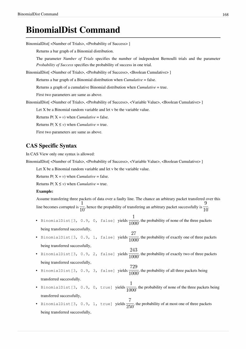
BinomialDist Command 168

BinomialDist CommandBinomialDist[ <Number of Trials>, <Probability of Success> ]

Returns a bar graph of a Binomial distribution.The parameter Number of Trials specifies the number of independent Bernoulli trials and the parameterProbability of Success specifies the probability of success in one trial.

BinomialDist[ <Number of Trials>, <Probability of Success>, <Boolean Cumulative> ]Returns a bar graph of a Binomial distribution when Cumulative = false.Returns a graph of a cumulative Binomial distribution when Cumulative = true.First two parameters are same as above.

BinomialDist[ <Number of Trials>, <Probability of Success>, <Variable Value>, <Boolean Cumulative> ]Let X be a Binomial random variable and let v be the variable value.Returns P( X = v) when Cumulative = false.Returns P( X ≤ v) when Cumulative = true.First two parameters are same as above.

CAS Specific SyntaxIn CAS View only one syntax is allowed:BinomialDist[ <Number of Trials>, <Probability of Success>, <Variable Value>, <Boolean Cumulative> ]

Let X be a Binomial random variable and let v be the variable value.Returns P( X = v) when Cumulative = false.Returns P( X ≤ v) when Cumulative = true.Example:

Assume transfering three packets of data over a faulty line. The chance an arbitrary packet transfered over this

line becomes corrupted is , hence the propability of transfering an arbitrary packet successfully is .

• BinomialDist[3, 0.9, 0, false] yields , the probability of none of the three packets

being transferred successfully,

• BinomialDist[3, 0.9, 1, false] yields , the probability of exactly one of three packets

being transferred successfully,

• BinomialDist[3, 0.9, 2, false] yields , the probability of exactly two of three packets

being transferred successfully,

• BinomialDist[3, 0.9, 3, false] yields , the probability of all three packets being

transferred successfully.

• BinomialDist[3, 0.9, 0, true] yields , the probability of none of the three packets being

transferred successfully,

• BinomialDist[3, 0.9, 1, true] yields , the probability of at most one of three packets

being transferred successfully,

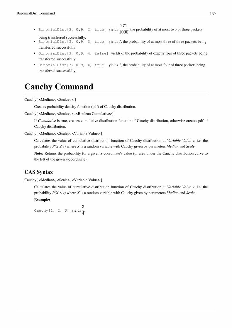
BinomialDist Command 169

• BinomialDist[3, 0.9, 2, true] yields , the probability of at most two of three packets

being transferred successfully,• BinomialDist[3, 0.9, 3, true] yields 1, the probability of at most three of three packets being

transferred successfully.• BinomialDist[3, 0.9, 4, false] yields 0, the probability of exactly four of three packets being

transferred successfully,• BinomialDist[3, 0.9, 4, true] yields 1, the probability of at most four of three packets being

transferred successfully.

Cauchy CommandCauchy[ <Median>, <Scale>, x ]

Creates probability density function (pdf) of Cauchy distribution.Cauchy[ <Median>, <Scale>, x, <Boolean Cumulative>]

If Cumulative is true, creates cumulative distribution function of Cauchy distribution, otherwise creates pdf ofCauchy distribution.

Cauchy[ <Median>, <Scale>, <Variable Value> ]Calculates the value of cumulative distribution function of Cauchy distribution at Variable Value v, i.e. theprobability P(X ≤ v) where X is a random variable with Cauchy given by parameters Median and Scale.Note: Returns the probability for a given x-coordinate's value (or area under the Cauchy distribution curve tothe left of the given x-coordinate).

CAS SyntaxCauchy[ <Median>, <Scale>, <Variable Value> ]

Calculates the value of cumulative distribution function of Cauchy distribution at Variable Value v, i.e. theprobability P(X ≤ v) where X is a random variable with Cauchy given by parameters Median and Scale.Example:

Cauchy[1, 2, 3] yields .

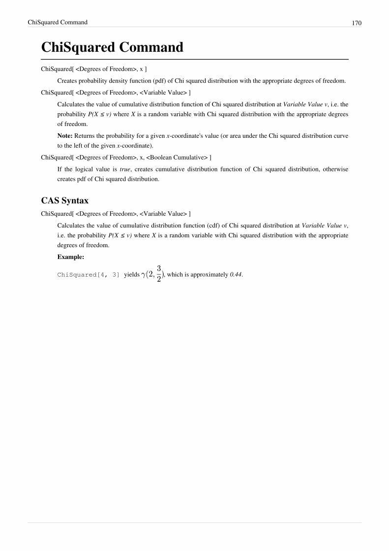
ChiSquared Command 170

ChiSquared CommandChiSquared[ <Degrees of Freedom>, x ]

Creates probability density function (pdf) of Chi squared distribution with the appropriate degrees of freedom.ChiSquared[ <Degrees of Freedom>, <Variable Value> ]

Calculates the value of cumulative distribution function of Chi squared distribution at Variable Value v, i.e. theprobability P(X ≤ v) where X is a random variable with Chi squared distribution with the appropriate degreesof freedom.Note: Returns the probability for a given x-coordinate's value (or area under the Chi squared distribution curveto the left of the given x-coordinate).

ChiSquared[ <Degrees of Freedom>, x, <Boolean Cumulative> ]If the logical value is true, creates cumulative distribution function of Chi squared distribution, otherwisecreates pdf of Chi squared distribution.

CAS SyntaxChiSquared[ <Degrees of Freedom>, <Variable Value> ]

Calculates the value of cumulative distribution function (cdf) of Chi squared distribution at Variable Value v,i.e. the probability P(X ≤ v) where X is a random variable with Chi squared distribution with the appropriatedegrees of freedom.Example:

ChiSquared[4, 3] yields , which is approximately 0.44.

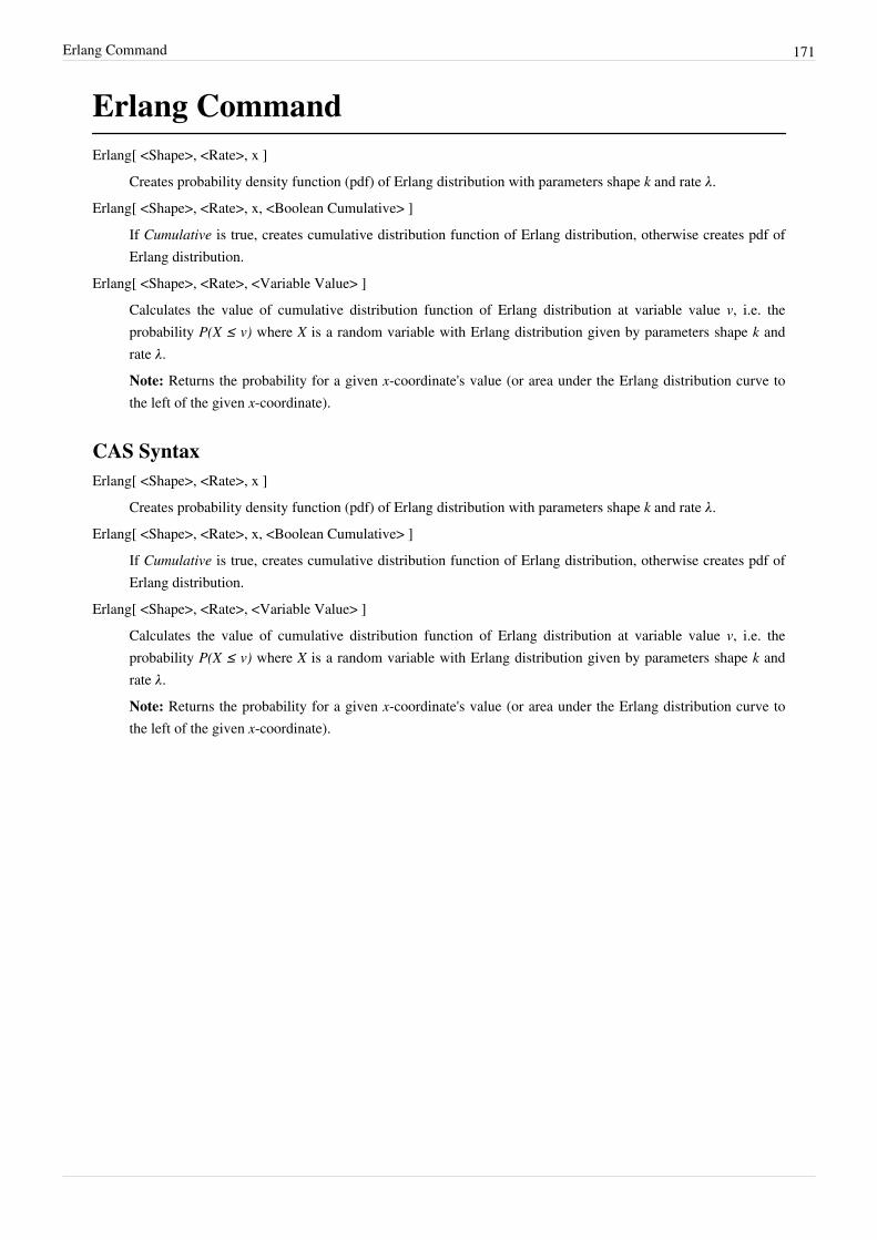
Erlang Command 171

Erlang CommandErlang[ <Shape>, <Rate>, x ]

Creates probability density function (pdf) of Erlang distribution with parameters shape k and rate λ.Erlang[ <Shape>, <Rate>, x, <Boolean Cumulative> ]

If Cumulative is true, creates cumulative distribution function of Erlang distribution, otherwise creates pdf ofErlang distribution.

Erlang[ <Shape>, <Rate>, <Variable Value> ]Calculates the value of cumulative distribution function of Erlang distribution at variable value v, i.e. theprobability P(X ≤ v) where X is a random variable with Erlang distribution given by parameters shape k andrate λ.Note: Returns the probability for a given x-coordinate's value (or area under the Erlang distribution curve tothe left of the given x-coordinate).

CAS SyntaxErlang[ <Shape>, <Rate>, x ]

Creates probability density function (pdf) of Erlang distribution with parameters shape k and rate λ.Erlang[ <Shape>, <Rate>, x, <Boolean Cumulative> ]

If Cumulative is true, creates cumulative distribution function of Erlang distribution, otherwise creates pdf ofErlang distribution.

Erlang[ <Shape>, <Rate>, <Variable Value> ]Calculates the value of cumulative distribution function of Erlang distribution at variable value v, i.e. theprobability P(X ≤ v) where X is a random variable with Erlang distribution given by parameters shape k andrate λ.Note: Returns the probability for a given x-coordinate's value (or area under the Erlang distribution curve tothe left of the given x-coordinate).

Exponential Command 172

Exponential CommandExponential[ <Lambda>, x ]

Creates probability density function (pdf) of exponential distribution with parameter lambda.Exponential[ <Lambda>, x, <Boolean Cumulative> ]

If Cumulative is true, creates cumulative distribution function (cdf) of exponential distribution, otherwisecreates pdf of Exponential distribution.

Exponential[ <Lambda>, <Variable Value> ]Calculates the value of cumulative distribution function of Exponential distribution at variable value v, i.e. theprobability P(X ≤ v) where X is a random variable with Exponential distribution with parameter lambda.Note: Returns the probability for a given x-coordinate's value (or area under the Exponential distribution curveto the left of the given x-coordinate).

CAS SyntaxExponential[ <Lambda>, <Variable Value> ]

Calculates the value of cumulative distribution function of exponential distribution at variable value v, i.e. theprobability P(X ≤ v) where X is a random variable with Exponential distribution with parameter lambda.Example:

Exponential[2, 1] yields , which is approximately 0.86.

FDistribution CommandFDistribution[ <Numerator Degrees of Freedom>, <Denominator Degrees of Freedom>, x ]

Creates probability density function (pdf) of F-distribution with parameters n, d (n for Numerator Degrees ofFreedom, d for Denominator Degrees of Freedom).

FDistribution[ <Numerator Degrees of Freedom>, <Denominator Degrees of Freedom>, x, <Boolean Cumulative> ]If Cumulative is true, creates cumulative distribution function of F-distribution, otherwise creates pdf ofF-distribution.

FDistribution[ <Numerator Degrees of Freedom>, <Denominator Degrees of Freedom>, <Variable Value> ]Calculates the value of cumulative distribution function of F-distribution at Variable Value v, i.e. theprobability P(X≤v) where X is a random variable with F-distribution given by parameters n, d (n forNumerator Degrees of Freedom, d for Denominator Degrees of Freedom).Note: Returns the probability for a given x-coordinate's value (or area under the F-distribution curve to the leftof the given x-coordinate).

FDistribution Command 173

CAS SyntaxFDistribution[ <Numerator Degrees of Freedom>, <Denominator Degrees of Freedom>, <Variable Value> ]

Calculates the value of cumulative distribution function of F-distribution at Variable Value v, i.e. theprobability P(X≤v) where X is a random variable with F-distribution given by parameters n, d (n forNumerator Degrees of Freedom, d for Denominator Degrees of Freedom).

Gamma CommandGamma[ <Number α>, <Number β>, x ]

Creates probability density function (pdf) of gamma distribution with parameters α, β.Gamma[ <Number α>, <Number β>, x, <Boolean Cumulative> ]

If Cumulative is true, creates cumulative distribution function of gamma distribution, otherwise creates pdf ofgamma distribution.

Gamma[ <Number α>, <Number β>, <Variable Value v> ]Calculates the value of cumulative distribution function of gamma distribution at v, i.e. the probability P(X≤v)where X is a random variable with gamma distribution given by parameters α, β.Note:

Returns the probability for a given x-coordinate's value (or area under the gamma distribution curve to the leftof the given x-coordinate).

CAS SyntaxGamma[ <Number α>, <Number β>, <Variable Value v> ]

Calculates the value of cumulative distribution function of gamma distribution at v, i.e. the probability P(X≤v)where X is a random variable with gamma distribution given by parameters α, β.

HyperGeometric Command 174

HyperGeometric CommandHyperGeometric[ <Population Size>, <Number of Successes>, <Sample Size>]

Returns a bar graph of a Hypergeometric distribution.Parameters:

Population size: number of balls in the urnNumber of Successes: number of white balls in the urnSample Size: number of balls drawn from the urn

The bar graph shows the probability function of the number of white balls in the sample.HyperGeometric[ <Population Size>, <Number of Successes>, <Sample Size>, <Boolean Cumulative> ]

Returns a bar graph of a Hypergeometric distribution when Cumulative = false.Returns the graph of a cumulative Hypergeometric distribution when Cumulative = true.First three parameters are same as above.

HyperGeometric[ <Population Size>, <Number of Successes>, <Sample Size>, <Variable Value>, <BooleanCumulative> ]

Let X be a Hypergeometric random variable and v the variable value.Returns P( X = v) when Cumulative = false.Returns P( X ≤ v) when Cumulative = true.First three parameters are same as above.

CAS SyntaxHyperGeometric[ <Population Size>, <Number of Successes>, <Sample Size>, <Variable Value>, <BooleanCumulative> ]

Let X be a Hypergeometric random variable and v the variable value.Returns P( X = v) when Cumulative = false.Returns P( X ≤ v) when Cumulative = true.The first three parameters are the same as above.Example:

Assume you select two balls out of ten balls, two of which are white, without putting any back.

• HyperGeometric[10, 2, 2, 0, false] yields , the probability of selecting zero white balls,

• HyperGeometric[10, 2, 2, 1, false] yields , the probability of selecting one white ball,

• HyperGeometric[10, 2, 2, 2, false] yields , the probability of selecting both white balls,• HyperGeometric[10, 2, 2, 3, false] yields 0, the probability of selecting three white balls.

• HyperGeometric[10, 2, 2, 0, true] yields , the probability of selecting zero (or less) white

balls,

• HyperGeometric[10, 2, 2, 1, true] yields , the probability of selecting one or less white

balls,

HyperGeometric Command 175

• HyperGeometric[10, 2, 2, 2, true] yields 1, the probability of selecting two or less whiteballs and

• HyperGeometric[10, 2, 2, 3, true] yields 1, the probability of selecting three or less whiteballs.

InverseBinomial CommandInverseBinomial[ <Number of Trials>, <Probability of Success>, <Probability> ]

Returns least integer n such that P(X ≤ n) ≥ p, where p is the probability and X is binomial random variablegiven by Number of Trials and Probability of Success.

Note: See also BinomialDist Command.

InverseCauchy CommandInverseCauchy[ <Median>, <Scale>, <Probability> ]

Computes the inverse of cumulative distribution function of Cauchy distribution at probability p, where theCauchy distribution is given by median m and scale s.In other words, finds t such that P(X ≤ t) = p, where X is Cauchy random variable.Probability p must be from [0,1].

InverseChiSquared CommandInverseChiSquared[ <Degrees of Freedom>, <Probability> ]

Computes the inverse of cumulative distribution function of Chi squared distribution at probability p, wherethe Chi squared distribution has given d degrees of freedom.In other words, finds t such that P(X ≤ t) = p, where X is Chi squared random variable.Probability p must be from [0,1].

InverseExponential Command 176

InverseExponential CommandInverseExponential[ <Lambda>, <Probability> ]

Computes the inverse of cumulative distribution function of exponential distribution at probability p, wherethe exponential distribution is given by Lambda.In other words, finds t such that P(X ≤ t) = p, where X is exponential random variable.Probability p must be from [0,1].

InverseFDistribution CommandInverseFDistribution[ <Numerator Degrees of Freedom>, <Denominator Degrees of Freedom>, <Probability> ]

Computes the inverse of cumulative distribution function of F-distribution at probability p, where theF-distribution is given by the degrees of freedom.In other words, finds t such that P(X ≤ t) = p, where X is random variable with F-distribution.Probability p must be from [0,1].

InverseGamma CommandInverseGamma[ <Alpha>, <Beta>, <Probability> ]

Computes the inverse of cumulative distribution function of gamma distribution at probability p, where thegamma distribution is given by parameters Alpha and Beta.In other words, finds t such that P(X ≤ t) = p, where X is random variable with gamma distribution.Probability p must be from [0,1].

InverseHyperGeometric Command 177

InverseHyperGeometric CommandInverseHyperGeometric[ <Population Size>, <Number of Successes>, <Sample Size>, <Probability> ]

Returns least integer n such that P(X ≤ n) ≥ p, where p is the probability and X is hypergeometric randomvariable given by Population Size, Number of Successes and Sample Size.

Note: See also HyperGeometric Command.

InverseNormal CommandInverseNormal[ <Mean>, <Standard Deviation>, <Probability> ]

Calculates the function with given probability P, mean μ and standard deviation σ, whereis the inverse of the cumulative distribution function Φ for N(0,1).

Note: Returns the x-coordinate with the given probability to the left under the normal distribution curve.

InversePascal CommandInversePascal[ <Number of Successes>, <Probability of Success>, <Probability> ]

Returns least integer n such that P(X≤n) ≥ p, where p is the probability and X is Pascal random variable [1]

given by Number of Successes and Probability of Success.Note: See also Pascal Command.

InversePoisson Command 178

InversePoisson CommandInversePoisson[ <Mean>, <Probability> ]

Returns least integer n such that P(X≤n) ≥ p, where p is the probability and X is Poisson random variable withmean λ.

Note: See also Poisson Command.

InverseTDistribution CommandInverseTDistribution[ <Degrees of Freedom>, <Probability> ]

Computes the inverse of cumulative distribution function of t-distribution at p, where the t-distribution has ddegrees of freedom. In other words, finds r such that P(X≤r)=p, where X is random variable witht-distribution. Probability p must be from [0,1].

InverseWeibull CommandInverseWeibull[ <Shape>, <Scale>, <Probability> ]

Computes the inverse of cumulative distribution function of Weibull distribution at p, where the Weibulldistribution is given by shape parameter k and scale parameter λ. In other words, finds t such that P(X ≤ t) = p,where X is random variable with Weibull distribution. Probability p must be from [0,1].

InverseZipf CommandInverseZipf[ <Number of Elements>, <Exponent>, <Probability> ]

Returns least integer n such that P(X≤n) ≥ p, where X is Zipf random variable given by Number of Elementsand Exponent and p is the probability.

Note: See also Zipf Command.

LogNormal Command 179

LogNormal CommandLogNormal[ <Mean>, <Standard Deviation>, x ]

Creates probability density function (pdf) of log-normal distribution with parameters mean μ and standarddeviation σ.

LogNormal[ <Mean>, <Standard Deviation>, x, <Boolean Cumulative> ]If Cumulative is true, creates cumulative density function of log-normal distribution, otherwise creates pdf oflog-normal distribution.

LogNormal[ <Mean>, <Standard Deviation>, <Variable Value> ]Calculates the value of cumulative distribution function of log-normal distribution at variable value v, i.e. theprobability P(X ≤ v) where X is a random variable with log-normal distribution given by parameters mean μand standard deviation σ.Note: Returns the probability for a given x-coordinate's value (or area under the log-normal distribution curveto the left of the given x-coordinate).

CAS SyntaxLogNormal[ <Mean>, <Standard Deviation>, x ]

Creates probability density function (pdf) of log-normal distribution with parameters mean μ and standarddeviation σ.

LogNormal[ <Mean>, <Standard Deviation>, x, <Boolean Cumulative> ]If Cumulative is true, creates cumulative density function of log-normal distribution, otherwise creates pdf oflog-normal distribution.

LogNormal[ <Mean>, <Standard Deviation>, <Variable Value> ]Calculates the value of cumulative distribution function of log-normal distribution at variable value v, i.e. theprobability P(X ≤ v) where X is a random variable with log-normal distribution given by parameters mean μand standard deviation σ.Note: Returns the probability for a given x-coordinate's value (or area under the log-normal distribution curveto the left of the given x-coordinate).

Logistic Command 180

Logistic CommandLogistic[ <Mean>, <Scale>, x ]

Creates probability density function (pdf) of logistic distribution with parameters mean μ and scale s.Logistic[ <Mean>, <Scale>, x, <Boolean Cumulative> ]

If Cumulative is true, creates cumulative distribution function of logistic distribution, otherwise creates pdf oflogistic distribution.

Logistic[ <Mean>, <Scale>, <Variable Value> ]Calculates the value of cumulative distribution function of logistic distribution at variable value v, i.e. theprobability P(X ≤ v) where X is a random variable with logistic distribution given by parameters mean μ andscale s.Note: Returns the probability for a given x-coordinate's value (or area under the logistic distribution curve tothe left of the given x-coordinate).

CAS SyntaxLogistic[ <Mean>, <Scale>, x ]

Creates probability density function (pdf) of logistic distribution with parameters mean μ and scale s.Logistic[ <Mean>, <Scale>, x, <Boolean Cumulative> ]

If Cumulative is true, creates cumulative distribution function of logistic distribution, otherwise creates pdf oflogistic distribution.

Logistic[ <Mean>, <Scale>, <Variable Value> ]Calculates the value of cumulative distribution function of logistic distribution at variable value v, i.e. theprobability P(X ≤ v) where X is a random variable with logistic distribution given by parameters mean μ andscale s.Note: Returns the probability for a given x-coordinate's value (or area under the logistic distribution curve tothe left of the given x-coordinate).

Normal Command 181

Normal CommandNormal[ <Mean>, <Standard Deviation>, x ]

Creates probability density function (pdf) of normal distribution.Normal[ <Mean>, <Standard Deviation>, x, <Boolean Cumulative> ]

If Cumulative is true, creates cumulative distribution function of normal distribution with mean μ and standarddeviation σ, otherwise creates pdf of normal distribution.

Normal[ <Mean μ>, <Standard Deviation σ>, <Variable Value v> ]

Calculates the function at v where Φ is the cumulative distribution function for N(0,1) with mean

μ and standard deviation σ.Note: Returns the probability for a given x-coordinate's value (or area under the normal distribution curve tothe left of the given x-coordinate).

CAS SyntaxNormal[ <Mean>, <Standard Deviation>, <Variable Value> ]

Calculates the function where Φ is the cumulative distribution function for N(0,1) with mean μ

and standard deviation σ.Example:

Normal[2, 0.5, 1] yields .

Pascal Command 182

Pascal CommandPascal[ <Number of Successes>, <Probability of Success> ]

Returns a bar graph of a Pascal distribution [1].Parameters:

Number of Successes: number of independent Bernoulli trials that must be successfulProbability of Success: probability of success in one trial

Pascal[ <Number of Successes>, <Probability of Success>, <Boolean Cumulative> ]Returns a bar graph of a Pascal distribution when Cumulative = false.Returns a graph of a cumulative Pascal distribution when Cumulative = true.First two parameters are same as above.

Pascal[ <Number of Successes>, <Probability of Success>, <Variable Value>, <Boolean Cumulative> ]Let X be a Pascal random variable and v the variable value.Returns P( X = v) when Cumulative = false.Returns P( X ≤ v) when Cumulative = true.First two parameters are same as above.

CAS SyntaxPascal[ <Number of Successes>, <Probability of Success>, <Variable Value>, <Boolean Cumulative> ]

Let X be a Pascal random variable.Returns P( X = v) when Cumulative = false.Returns P( X ≤ v) when Cumulative = true.Example:

The number of independent Bernoulli trials that must be successful is n = 1, the probability of success in one

trial is p = , the variable value is v = 2 and "Cumulative" = false.

Pascal[ n, p, v, false] yields

Poisson Command 183

Poisson CommandPoisson[ <Mean> ]

Returns a bar graph of a Poisson distribution with given mean λ.Poisson[ <Mean>, <Boolean Cumulative> ]

Returns a bar graph of a Poisson distribution when Cumulative = false.Returns a graph of a cumulative Poisson distribution when Cumulative = true.The first parameter is same as above.

Poisson[ <Mean>, <Variable Value v>, <Boolean Cumulative> ]Let X be a Poisson random variable.Returns P( X = v) when Cumulative = false.Returns P( X ≤ v) when Cumulative = true.First parameter is same as above.

CAS SyntaxPoisson[ <Mean>, <Variable Value v>, <Boolean Cumulative> ]

Let X be a Poisson random variable.Returns P( X = v) when Cumulative = false.Returns P( X ≤ v) when Cumulative = true.First parameter is same as above.Examples:

• Poisson[3, 1, true] yields .• Poisson[3, 1, false] yields .

RandomBetween Command 184

RandomBetween CommandRandomBetween[ <Minimum Integer> , <Maximum Integer> ]

Generates a random integer between minimum and maximum (inclusive).Example:

RandomBetween[0, 10] yields a number between 0 and 10 (inclusive)RandomBetween[ <Minimum Integer> , <Maximum Integer> , <Boolean Fixed> ]

If Boolean Fixed = "true", it generates a random integer between minimum and maximum (inclusive), which isupdated just once (when file is loaded and also on undo/redo).Example:

RandomBetween[0, 10, true] yields a number between 0 and 10 (inclusive)Note: Press F9 to see the difference between those two syntaxes.

CAS SyntaxRandomBetween[ <Minimum Integer> , <Maximum Integer> ]

Generates a random integer between minimum and maximum (inclusive).Example:

RandomBetween[0, 10] yields a number between 0 and 10 (inclusive)Note: See also SetSeed command, RandomElement command, RandomBinomial command, RandomNormalcommand, RandomPoisson command, RandomUniform command.

RandomBinomial Command 185

RandomBinomial CommandRandomBinomial[ <Number of Trials>, <Probability> ]

Generates a random number from a binomial distribution with n trials and probability p.Example:

RandomBinomial[3, 0.1] gives j ∈ {0, 1, 2, 3}, where the probability of getting j is the probability of anevent with probability 0.1 occuring j times in three tries.

CAS SyntaxRandomBinomial[ <Number of Trials>, <Probability> ]

Generates a random number from a binomial distribution with n trials and probability p.Example:

RandomBinomial[3, 0.1] gives j ∈ {0, 1, 2, 3}, where the probability of getting j is the probability of anevent with probability 0.1 occuring j times in three tries.

Note: See also SetSeed command, RandomBetween command, RandomElement command, RandomNormalcommand, RandomPoisson command, RandomUniform command.

RandomNormal CommandRandomNormal[ <Mean>, <Standard Deviation> ]

Generates a random number from a normal distribution with given mean and standard deviation.Example:

RandomNormal[3, 0.1] yields a random value from a normal distribution with a mean of 3 and standarddeviation of 0.1.

CAS SyntaxRandomNormal[ <Mean>, <Standard Deviation> ]

Generates a random number from a normal distribution with given mean and standard deviation.Example:

RandomNormal[3, 0.1] yields a random value from a normal distribution with a mean of 3 and standarddeviation of 0.1.

Note: See also SetSeed command, RandomBetween command, RandomElement command, RandomBinomialcommand, RandomPoisson command, RandomUniform command.

RandomPoisson Command 186

RandomPoisson CommandRandomPoisson[ <Mean> ]

Generates a random number from a Poisson distribution with given mean.Example:

RandomPoisson[3] yields a random value from a Poisson distribution with a mean of 3.

CAS SyntaxRandomPoisson[ <Mean> ]

Generates a random number from a Poisson distribution with given mean.Example:

RandomPoisson[3] yields a random value from a Poisson distribution with a mean of 3.Note: See also SetSeed command, RandomBetween command, RandomElement command, RandomBinomialcommand, RandomNormal command, RandomUniform command.

RandomUniform CommandRandomUniform[ <Min>, <Max> ]

Returns random real number from uniform distribution on interval [min, max].Example:

RandomUniform[0, 1] returns a random number between 0 and 1RandomUniform[ <Min>, <Max>, <Number of Samples n> ]

Returns a list of n random real numbers from uniform distribution on interval [min, max].Example:

RandomUniform[0, 1, 3] returns a list of three random numbers between 0 and 1

CAS SyntaxRandomUniform[ <Min>, <Max> ]

Returns random real number from uniform distribution on interval [min, max].Example:

RandomUniform[0, 1] returns a random number between 0 and 1Note: RandomUniform[0,1] is equivalent to random() (see Predefined Functions and Operators).Note: See also SetSeed, RandomBetween, RandomElement, RandomBinomial, RandomNormal , RandomPoissoncommands.

TDistribution Command 187

TDistribution CommandTDistribution[ <Degrees of Freedom>, x ]

Creates probability density function (pdf) of t-distribution with given degrees of freedom.TDistribution[ <Degrees of Freedom>, x, <Boolean Cumulative> ]

If Cumulative is true, creates cumulative distribution function of t-distribution, otherwise creates pdf oft-distribution.

TDistribution[ <Degrees of Freedom>, <Variable Value> ]Calculates the value of cumulative distribution function of t-distribution at variable value v, i.e. the probabilityP(X ≤ v) where X is a random variable with t-distribution with given degrees of freedom.Example:

TDistribution[10, 0] yields 0.5.Note: Returns the probability for a given x-coordinate's value (or area under the t-distribution curve to the leftof the given x-coordinate).

CAS SyntaxTDistribution[ <Degrees of Freedom>, <Variable Value> ]

Calculates the value of cumulative distribution function of t-distribution at variable value v, i.e. the probabilityP(X ≤ v) where X is a random variable with t-distribution with given degrees of freedom.Example:

TDistribution[10, 0] yields .

Triangular Command 188

Triangular CommandTriangular[ <Lower Bound>, <Upper Bound>, <Mode>, x ]

Creates probability density function of triangular distribution with parameters min, max, mod.Triangular[ <Lower Bound>, <Upper Bound>, <Mode>, x, <Boolean Cumulative> ]

If Cumulative is true, creates cumulative distribution function of triangular distribution, otherwise createsprobability density function of triangular distribution.

Triangular[ <Lower Bound>, <Upper Bound>, <Mode>, <Variable Value> ]Calculates the value of cumulative distribution function of triangular distribution at Variable Value v, i.e. theprobability P(X≤v) where X is a random variable with triangular distribution given by parameters min, max,mod.Note: Returns the probability for a given x-coordinate's value (or area under the triangular distribution curve tothe left of the given x-coordinate).

CAS SyntaxTriangular[ <Lower Bound>, <Upper Bound>, <Mode>, <Variable Value>]

Calculates the value of cumulative distribution function of triangular distribution at Variable Value v, i.e. theprobability P(X≤v) where X is a random variable with triangular distribution given by parameters min, max,mod.Example:

Triangular[ 0, 5, 2, 2 ] yields 0.4.

Uniform Command 189

Uniform CommandUniform[ <Lower Bound min>, <Upper Bound max>, x ]

Returns the probability density function of uniform distribution on interval [min,max].Uniform[ <Lower Bound min>, <Upper Bound max>, x, <Boolean Cumulative b> ]

For b=false returns the probability density function of uniform distribution on interval [min,max].For b=true returns the cumulative distribution function of the same distribution.

Uniform[ <Lower Bound min>, <Upper Bound max>, <Variable Value v> ]Returns the value of cumulative distribution function at v (i.e. P(X<v)) for uniform distribution on interval[min,max]

Weibull CommandWeibull[ <Shape>, <Scale>, x ]

Creates probability density function (pdf) of Weibull distribution with parameters shape k and scale λWeibull[ <Shape>, <Scale>, x, <Boolean Cumulative> ]

If Cumulative is true, creates cumulative distribution function of Weibull distribution, otherwise creates pdf ofWeibull distribution.

Weibull[ <Shape>, <Scale>, <Variable Value> ]Calculates the value of cumulative distribution function of Weibull distribution at variable value v, i.e. theprobability P(X ≤ v) where X is a random variable with Weibull distribution given by parameters shape k andscale λ.Note: Returns the probability for a given x-coordinate's value (or area under the Weibull distribution curve tothe left of the given x-coordinate).

CAS SyntaxWeibull[ <Shape>, <Scale>, <Variable Value> ]

Calculates the value of cumulative distribution function of Weibull distribution at variable value v, i.e. theprobability P(X ≤ v) where X is a random variable with Weibull distribution given by parameters shape k andscale λ.Examples:

• Weibull[ 0.5, 1, 0] yields 0.

• Weibull[ 0.5, 1, 1] yields .

Zipf Command 190

Zipf CommandZipf[ <Number of Elements>, <Exponent> ]

Returns a bar graph of a Zipf distribution.Parameters:

• Number of Elements: number of elements whose rank we study• Exponent: exponent characterizing the distribution

Zipf[ <Number of Elements>, <Exponent> , <Boolean Cumulative> ]Returns a bar graph of a Zipf distribution when Cumulative = false.Returns a graph of a cumulative Zipf distribution when Cumulative = true.First two parameters are same as above.

Zipf[ <Number of Elements>, <Exponent> , <Variable Value v>, <Boolean Cumulative> ]Let X be a Zipf random variable.Returns P( X = v) when Cumulative = false.Returns P( X ≤ v) when Cumulative = true.First two parameters are same as above.

CAS SyntaxZipf[ <Number of Elements>, <Exponent> , <Variable Value v>, <Boolean Cumulative> ]

Let X be a Zipf random variable.Returns P( X = v) when Cumulative = false.Returns P( X ≤ v) when Cumulative = true.Example:

Zipf[ 10, 1 , 5, false] yields .

Spreadsheet Commands 191

Spreadsheet CommandsThese commands are designed for referencing data from Spreadsheet View and copying data into it.•• Cell•• CellRange•• Column•• ColumnName•• FillCells•• FillColumn•• FillRow•• Row

Cell CommandCell[ <Column>, <Row> ]

Returns copy of spreadsheet cell in given column and row.Example: Cell[2, 1] returns copy of B1.

Note:

• By default the cells in spreadsheet cells are auxiliary and in such case this command returns auxiliary object aswell.

• You must make sure that the cells you refer to are earlier in the Construction Protocol than this command.

CellRange Command 192

CellRange CommandCellRange[ <Start Cell>, <End Cell> ]

Creates a list containing the cell values in this cell range.Example:

Let A1 = 1, A2 = 4, A3 = 9 be spreadsheet cells values.Then CellRange[A1, A3] returns the list{1, 4, 9}.

Note: A1:A3 is a shorter syntax.

Column CommandColumn[ <Spreadsheet Cell> ]

Returns the column of the cell as a number (starting at 1).Example: q = Column[B3] returns q = 2 since column B is the second column of the spreadsheet.

ColumnName CommandColumnName[ <Spreadsheet Cell> ]

Returns the column name of the cell as a text.Example: r = ColumnName[A1] creates r = A and shows such text - A - in the Graphics View.

FillCells Command 193

FillCells CommandFillCells[ <CellRange>, <Object> ]

Copies the value/equation etc. of the object to the given cellrange. Resulting cells are free objects, i.e.independent of object.Notes:CellRange has to be entered like this: e.g.: B2:D5.Object can be anything, e.g.: 3, RandomBetween[0,10], Circle[A, B].Cells are labelled by column and row, e.g.: B2

FillCells[ <Cell>, <List> ]Copies values from the list to the first cells on the right of the given cell. Resulting cells are free objects, i.e.independent of the list.

FillCells[ <Cell>, <Matrix> ]Copies values from the matrix. The upper left corner of the matrix is matched to the given cell. Resulting cellsare free objects, i.e. independent of the matrix.

Note: See also FillRow and FillColumn commands.

FillColumn CommandFillColumn[ <Column>, <List> ]

Copies values from the list to the first cells of the column given by number (1 for A, 2 for B, etc.). Resultingcells are free objects, i.e. independent of the list.

Note: See also the FillRow and FillCells commands.

FillRow Command 194

FillRow CommandFillRow[ <Row>, <List> ]

Copies values from the list to the first cells of the row given by number. Resulting cells are free objects, i.e.independent of the list.

Note: See also the FillColumn and FillCells commands.

Row CommandRow[ <Spreadsheet Cell> ]

Returns the row number of the spreadsheet cell (starting at 1).Example: r = Row[B3] yields r = 3.

Scripting CommandsThese commands are substitutes for features accessible e.g. via Properties Dialog and are meant to simplify scriptingin GeoGebra.Note: These commands don't return any object, therefore cannot be nested in other commands.•• AttachCopyToView•• Button•• CenterView•• Checkbox•• CopyFreeObject•• Delete•• Execute•• GetTime•• HideLayer•• InputBox•• Pan•• ParseToFunction•• ParseToNumber•• PlaySound•• Rename•• SelectObjects•• SetActiveView•• SetAxesRatio•• SetBackgroundColor•• SetCaption•• SetColor•• SetConditionToShowObject•• SetCoords•• SetDynamicColor•• SetFilling•• SetFixed

Scripting Commands 195

•• SetLabelMode•• SetLayer•• SetLineStyle•• SetLineThickness•• SetPointSize•• SetPointStyle•• SetSeed•• SetTooltipMode•• SetTrace•• SetValue•• SetVisibleInView•• ShowAxes•• ShowGrid•• ShowLabel•• ShowLayer•• Slider•• StartAnimation•• UpdateConstruction•• ZoomIn•• ZoomOut

Button CommandButton[ ]

Creates a new button.Button[ <Caption> ]

Creates a new button with given caption.

Checkbox Command 196

Checkbox CommandCheckbox[ ]

Creates a checkbox.Checkbox[ <Caption> ]

Creates a checkbox with given caption.Checkbox[ <List> ]

Creates a checkbox which, when unchecked, hides listed objects.Example: Let A and B be points. c = Checkbox[{A,B}] creates checkbox c. When c is checked, A andB are visible, otherwise they are hidden.

Checkbox[ <Caption>, <List> ]Creates checkbox with given caption which, when unchecked, hides listed objects.

CopyFreeObject CommandCopyFreeObject[ <Object> ]

Creates a free copy of the object. Preserves all basic Object Properties and copy of Auxiliary Object isauxiliary as well.

Delete CommandDelete[ <Object> ]

Deletes the object and all its dependent objects.Example: Delete[a] clears a.

CAS SyntaxDelete[ <Object> ]

Deletes the object and all its dependent objects in GeoGebra and removes any value assigned to the object inthe CAS.Example: Delete[a] clears a.

Note: See also Delete tool.

Execute Command 197

Execute CommandExecute[ <List of Texts> ]

Executes list of commands entered as texts.Note: Please note that you always need to use English commands within this list of texts, no matter which languageoption you selected for GeoGebra.

Examples:Execute[{"A=(1,1)","B=(3,3)","C = Midpoint[A, B]"}] creates points A, B and their midpointC.Execute[Join[{"f_{1} = 1", "f_{2} = 1"}, Sequence["f_{"+(i + 2) + "} = f_{" + (i+1) + "} + f_{"+ i +"}", i,1, 10]]] creates first 10 elements of Fibonacci sequence.

Execute[ <List of Texts>, <Parameter>, ... , <Parameter> ]Replaces %1 for the first parameter, %2 for the second parameter and so on in each text in list. Up to 9parameters can be specified. After the replacement, resulting scripts are executed.Example:Execute[{"Midpoint[%1,%2]"},A,B] creates midpoint of segment AB.Note: Command names must be in English in the texts for this command to work.

GetTime CommandGetTime[]

Returns a list with the current time and date in this order:milliseconds, seconds, minutes, hours (0-23), date, month (1-12), year, month (as text), day (as text), day (1 =Sunday, 2 = Monday, etc)Example: GetTime[] returns a list such as {647, 59, 39, 23, 28, 2, 2011, "February", "Monday", 2}

GetTime[ "<Format>" ]where Format is a Text, replaces any of the following characters when prefixed by a backslash (\):d, D, j, l, N, S, w, z, W, F, m, M, n, t, L, Y, y, a, A, g, G, h, H, i, s, U - the explanation to these characters arehere http:/ / php. net/ manual/ en/ function. date. phpExample: GetTime["The date is \l the \j\S of \F \Y"] might give The date is Thursdaythe 5th of July 2012

HideLayer Command 198

HideLayer CommandHideLayer[ <Number> ]

Makes all objects in given layer invisible. Does not override Conditional Visibility.

Pan CommandPan[ <x>, <y> ]

Shifts the current view by x pixels to the left and y pixels upwards.Pan[ <x>, <y>, <z> ]

Shifts the current view by (x, y, z) if it's a 3D View, or just by (x,y) for a 2D ViewNotes:If multiple Graphics ViewGraphics Views are present, the active one is used See also ZoomInCommandZoomIn, ZoomOut CommandZoomOut, SetActiveView CommandSetActiveView commands.

ParseToFunction CommandParseToFunction[ <Function>, <String> ]

Parses the string and stores the result to a function f, which must be defined and free before the command isused.Example: Define f(x) = 3x² + 2 and text1 = "f(x) = 3x + 1". ParseToFunction[f,text1] returns f(x) = 3x + 1.

Note: See also ParseToNumber command.

ParseToNumber Command 199

ParseToNumber CommandParseToNumber[ <Number>, <String> ]

Parses the string and stores the result to a number a, which must be defined and free before the command isused.Example: Define a = 3 and text1 = "6". ParseToNumber[a, text1] returns a = 6.

Note: See also ParseToFunction command.

Plane CommandPlane[ <Polygon> ]

Creates a plane through the polygon.Plane[ <Conic> ]

Creates a plane through the conic.Plane[ <Point>, <Plane> ]

Creates a plane through the given point, parallel to the given plane.Plane[ <Point>, <Line> ]

Creates a plane through the given point and line.Plane[ <Line> , <Line> ]

Creates the plane through the lines (if the lines are in the same plane).Plane[ <Point>, <Point>, <Point> ]

Creates a plane through three points.

Note: See also Plane through 3 Points and Plane tools.

PlaySound Command 200

PlaySound CommandPlaySound[ <Note>, <Duration>, <Instrument> ]

Plays a MIDI note.Note is an integer from 0 to 127 that represents a musical note given by the table below. When note = 60 aMiddle C is played.Duration is the time to play the note in seconds.Instrument is an integer that represents the synthesized instrument used to play the note. See technicalspecifications [1] for possible instruments.Most instruments are supported, but there are differences between computer platforms.

MIDI NotesOctave C C# D D# E F F# G G# A A# + 0 0 1 2 3 4 5 6 7 8 9 10 + 1 12 13 14 15 16 17 18 19 20 21 22 + 2 24 25 26 27 28 29 30 31 32 33 34 + 3 36 37 38 39 40 41 42 43 44 45 46 + 4 48 49 50 51 51 53 54 55 56 57 58 + 5 60 61 62 63 64 65 66 67 68 69 70 + 6 72 73 74 75 76 77 78 79 80 81 82 + 7 84 85 86 87 88 89 90 91 92 93 94 + 8 96 97 98 99 100 101 102 103 104 105 106 + 9 108 109 110 111 112 113 114 115 116 117 118 + 10 120 121 122 123 124 125 126 127 +

PlaySound[ <Note Sequence>, <Instrument> ]Plays a sequence of MIDI notes and commands using a JFugue [2] music string.Note Sequence is a text string that uses JFugue character commands.Instrument is the default MIDI instrument used when the string is played.The basic commands are given below. The full command set is described inThe Complete Guide to JFugue [3] (English).

Basic JFugue Commands

Character + A-G + [number] + + + R + w, h, q,i, s

+ /n + I[number] + V + Space Play the previous note, combination ofnotes or rest.

Example: PlaySound["C+E+G Rw Ai Bi Ci A4i B4i C4i ", 0] Plays a quarter note chord CEG;rests for a whole note; plays the eighth notes A, B, C; plays them again one octave lower. Piano instrument is used.Example: PlaySound["I[56] C5q D5q I[71] G5q F5q", 0] Plays notes with different instruments.Trumpet = 56 and Clarinet = 71.Example: PlaySound["V0 A3q B3q C3q B3q V1 A2h C2h", 0] Plays notes in harmony withdifferent voices.PlaySound[ <File> ]

Plays a MIDI file (*.mid) or a text file (* .txt) containing a JFugue string."File" is the directory path to this file, e.g. PlaySound["path/to/myFile.mid"]

PlaySound[ <Function>, <Min Value>, <Max Value> ]Plays a sound generated by Function, a time-valued function with range [-1,1]. The time units are seconds andthe sound is played from time Min Value to Max Value. Sound is generated by 8-bit samples taken at a rate of8000 samples per second.

Example: PlaySound[sin(440 2Pi x), 0, 1]This plays a pure sine wave tone at 440 Hz (musical noteA) for one second.PlaySound[ <Function>, <Min Value>, <Max Value>, <Sample Rate>, <Sample Depth> ]

PlaySound Command 201

Plays a sound generated by Function, a time-valued function with range [-1,1]. The time units are seconds andthe sound is played from time Min Value to Max Value. The sampling method is specified by "Sample Depth"and "Sample Rate"."Sample Rate" is the number of sample function values taken each second. Allowable values are 8000, 11025,16000, 22050, or 44100"Sample Depth" is the data size of a sample in bits. Allowable values are 8 and 16.

PlaySound[ <Boolean Play> ]Pause or resume play.PlaySound[true] = play, PlaySound[false] = pause.

Rename CommandRename[ <Object>, <Name> ]

Sets the label of given object to the given name.Example:

Let c: x^2 + 2y^2 = 2.Rename[c, ell] sets the label to ell.

SelectObjects CommandSelectObjects[ ]

Deselects all selected objects.SelectObjects[ <Object>, <Object>, ... ]

Deselects all objects and selects objects passed as parameters. All parameters must be labeled objects.Examples:

• Let A, B and C be points. SelectObjects[A, B, C] selects points A, B and C.• The command SelectObjects[Midpoint[A, B]] has no effect.

Note: This command now cancels any drag that is in progress (useful in scripts).

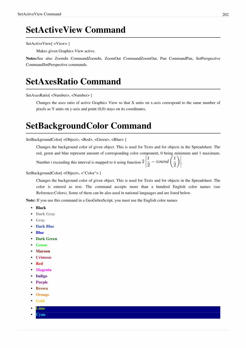
SetActiveView Command 202

SetActiveView CommandSetActiveView[ <View> ]

Makes given Graphics View active.Notes:See also ZoomIn CommandZoomIn, ZoomOut CommandZoomOut, Pan CommandPan, SetPerspectiveCommandSetPerspective commands.

SetAxesRatio CommandSetAxesRatio[ <Number>, <Number> ]

Changes the axes ratio of active Graphics View so that X units on x-axis correspond to the same number ofpixels as Y units on y-axis and point (0,0) stays on its coordinates.

SetBackgroundColor CommandSetBackgroundColor[ <Object>, <Red>, <Green>, <Blue> ]

Changes the background color of given object. This is used for Texts and for objects in the Spreadsheet. Thered, green and blue represent amount of corresponding color component, 0 being minimum and 1 maximum.

Number t exceeding this interval is mapped to it using function .

SetBackgroundColor[ <Object>, <"Color"> ]Changes the background color of given object. This is used for Texts and for objects in the Spreadsheet. Thecolor is entered as text. The command accepts more than a hundred English color names (seeReference:Colors). Some of them can be also used in national languages and are listed below.

Note: If you use this command in a GeoGebraScript, you must use the English color names•• Black•• Dark Gray•• Gray•• Dark Blue•• Blue•• Dark Green•• Green•• Maroon•• Crimson•• Red•• Magenta•• Indigo•• Purple•• Brown•• Orange•• Gold

•• Lime•• Cyan

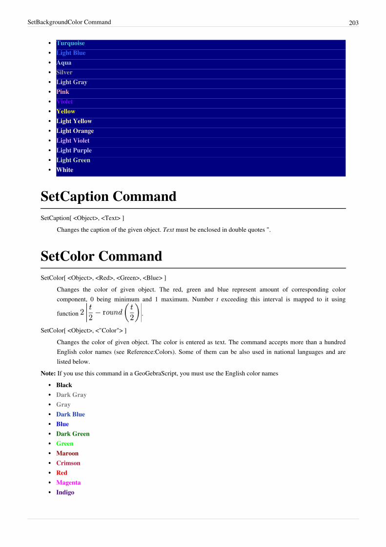
SetBackgroundColor Command 203

•• Turquoise•• Light Blue•• Aqua•• Silver•• Light Gray•• Pink•• Violet•• Yellow•• Light Yellow•• Light Orange•• Light Violet•• Light Purple•• Light Green•• White

SetCaption CommandSetCaption[ <Object>, <Text> ]

Changes the caption of the given object. Text must be enclosed in double quotes ".

SetColor CommandSetColor[ <Object>, <Red>, <Green>, <Blue> ]

Changes the color of given object. The red, green and blue represent amount of corresponding colorcomponent, 0 being minimum and 1 maximum. Number t exceeding this interval is mapped to it using

function .

SetColor[ <Object>, <"Color"> ]Changes the color of given object. The color is entered as text. The command accepts more than a hundredEnglish color names (see Reference:Colors). Some of them can be also used in national languages and arelisted below.

Note: If you use this command in a GeoGebraScript, you must use the English color names•• Black•• Dark Gray•• Gray•• Dark Blue•• Blue•• Dark Green•• Green•• Maroon•• Crimson•• Red•• Magenta•• Indigo

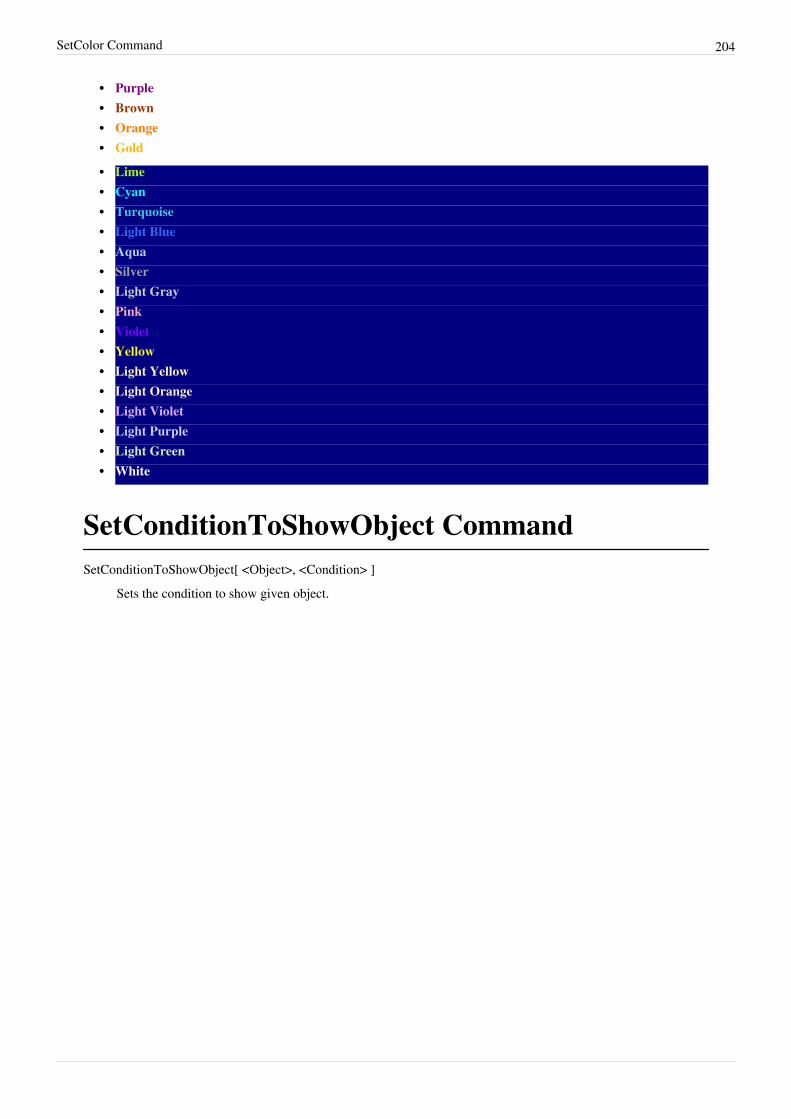
SetColor Command 204

•• Purple•• Brown•• Orange•• Gold

•• Lime•• Cyan•• Turquoise•• Light Blue•• Aqua•• Silver•• Light Gray•• Pink•• Violet•• Yellow•• Light Yellow•• Light Orange•• Light Violet•• Light Purple•• Light Green•• White

SetConditionToShowObject CommandSetConditionToShowObject[ <Object>, <Condition> ]

Sets the condition to show given object.

SetCoords Command 205

SetCoords CommandSetCoords[ <Object>, <x>, <y> ]

Changes cartesian coordinates of free objects. This command uses values of the coordinates, not theirdefinitions, therefore the object stays free.

Note: This command now works for Sliders, Buttons, Checkboxes, Input Boxes, Images. If "Absolute ScreenPosition" is selected then x, y are in screen pixels.

SetDynamicColor CommandSetDynamicColor[ <Object>, <Red>, <Green>, <Blue> ]

Sets the dynamic color of the object.SetDynamicColor[ <Object>, <Red>, <Green>, <Blue>, <Opacity> ]

Sets the dynamic color and opacity of the object.Note: All numbers are on a scale from 0 (off/transparent) to 1 (on/opaque)

SetFilling CommandSetFilling[ <Object>, <Number> ]

Changes the opacity of given object. Number must be from interval [0,1], where 0 means transparent and 1means 100% opaque. Other numbers are ignored.

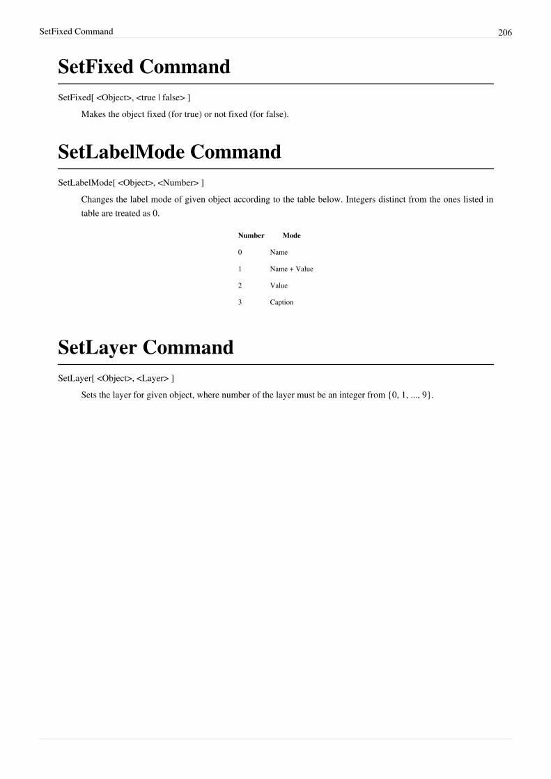
SetFixed Command 206

SetFixed CommandSetFixed[ <Object>, <true | false> ]

Makes the object fixed (for true) or not fixed (for false).

SetLabelMode CommandSetLabelMode[ <Object>, <Number> ]

Changes the label mode of given object according to the table below. Integers distinct from the ones listed intable are treated as 0.

Number Mode

0 Name

1 Name + Value

2 Value

3 Caption

SetLayer CommandSetLayer[ <Object>, <Layer> ]

Sets the layer for given object, where number of the layer must be an integer from {0, 1, ..., 9}.

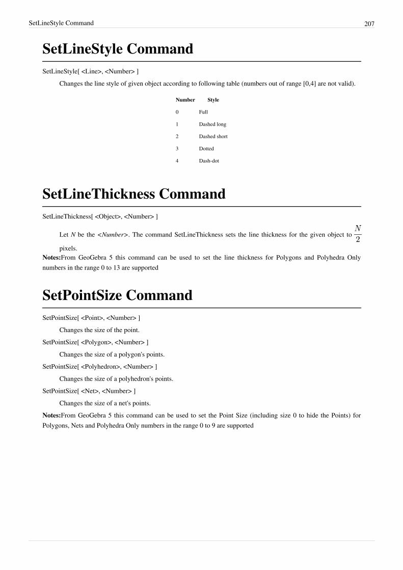
SetLineStyle Command 207

SetLineStyle CommandSetLineStyle[ <Line>, <Number> ]

Changes the line style of given object according to following table (numbers out of range [0,4] are not valid).

Number Style

0 Full

1 Dashed long

2 Dashed short

3 Dotted

4 Dash-dot

SetLineThickness CommandSetLineThickness[ <Object>, <Number> ]

Let N be the <Number>. The command SetLineThickness sets the line thickness for the given object to

pixels.Notes:From GeoGebra 5 this command can be used to set the line thickness for Polygons and Polyhedra Onlynumbers in the range 0 to 13 are supported

SetPointSize CommandSetPointSize[ <Point>, <Number> ]

Changes the size of the point.SetPointSize[ <Polygon>, <Number> ]

Changes the size of a polygon's points.SetPointSize[ <Polyhedron>, <Number> ]

Changes the size of a polyhedron's points.SetPointSize[ <Net>, <Number> ]

Changes the size of a net's points.Notes:From GeoGebra 5 this command can be used to set the Point Size (including size 0 to hide the Points) forPolygons, Nets and Polyhedra Only numbers in the range 0 to 9 are supported

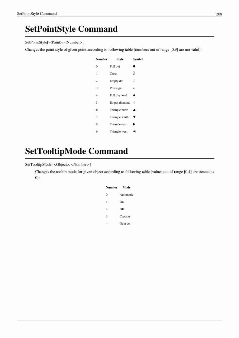
SetPointStyle Command 208

SetPointStyle CommandSetPointStyle[ <Point>, <Number> ]Changes the point style of given point according to following table (numbers out of range [0,9] are not valid).

Number Style Symbol

0 Full dot ●

1 Cross ⨯

2 Empty dot ○

3 Plus sign +

4 Full diamond ◆

5 Empty diamond ◇

6 Triangle north ▲

7 Triangle south ▼

8 Triangle east ▶

9 Triangle west ◀

SetTooltipMode CommandSetTooltipMode[ <Object>, <Number> ]

Changes the tooltip mode for given object according to following table (values out of range [0,4] are treated as0):

Number Mode

0 Automatic

1 On

2 Off

3 Caption

4 Next cell

SetValue Command 209

SetValue CommandSetValue[ <Boolean>, <0|1> ]

Sets the state of a boolean / check box : 1 = true, 0 = falseExample: If b is a boolean, SetValue[b,1] sets the boolean b as true.

SetValue[ <Object>, <Object> ]LetA be the first and B the second object. If A is a free object or a Point restricted to Path or Region, its valueis set to current value of B (i.e. A doesn't change value if B is changed afterwards).Example: If f is a function, SetValue[f, RandomElement[{cos(x), 3x+2, ln(x)}]] defines,at random, f as being one of the functions proposed in the list.

SetValue[ <List>, <Number>, <Object> ]Let n be the <Number>. The command SetValue sets the n-th element of a free list to the current value of theobject. Number n can be at most 1 + length of L.

SetVisibleInView CommandSetVisibleInView[ <Object>, <View Number 1|2>, <Boolean> ]

Makes object visible or hidden in given Graphics View.

ShowLabel CommandShowLabel[ <Object>, <Boolean> ]

Shows or hides the label in the Graphics View for the given object.Example:

Let f(x) = x^2.ShowLabel[f, true] shows the label of the function.

ShowLayer Command 210

ShowLayer CommandShowLayer[ <Number> ]

Makes all objects in given layer visible. Does not override Conditional Visibility.Example:

ShowLayer[2] makes all objects in the second layer visible.

Slider CommandSlider[ <Min>, <Max>, <Increment>, <Speed>, <Width>,<Is Angle>, <Horizontal>, <Animating>, <BooleanRandom>]

Creates a slider. The parameters settings can be as follows:• Min, Max: set the range of the slider - These parameters are compulsory.• Increment: set the increment of the slider's value - default: 0.1• Speed: set the slider speed during animations - default: 1• Width: sets the slider width in pixels - default: 100• Is Angle: sets if the slider is related to an angle. This parameter can be true or false - default: false• Horizontal: sets whether the slider is shown as an horizontal (true) or vertical (false) segment - default: true• Animating: sets the automatic animation of the slider - default: false• Random: sets if the slider assumes continuous values in the [Min, Max] range (false), or random values in the

same interval (true) - default: false

StartAnimation Command 211

StartAnimation CommandStartAnimation[ ]

Resumes all animations if they are paused.StartAnimation[ <Boolean> ]

When the boolean is false, pauses all animations, otherwise resumes them.StartAnimation[ <Point or Slider>, <Point or Slider>, .... ]

Starts animating given points and sliders, the points must be on paths.StartAnimation[ <Point or Slider>, <Point or Slider>, ...., <Boolean> ]

Starts (for boolean = true) or permanently stops (for boolean = false) animating given points and sliders, thepoints must be on paths.

Note: See also Animation.

InputBox CommandInputBox[]

Create a new Input Box.InputBox[ <Linked Object> ]

Create a new Input Box and associate a Linked Object with it.

Note: See also Input Box Tool.

UpdateConstruction Command 212

UpdateConstruction CommandUpdateConstruction[ ]

Recomputes all objects (random numbers are regenerated). Same as F9 or Ctrl + R.Note: If you want to refresh the view (e.g to remove traces from Graphics View) you can use ZoomIn[1] instead,which is the same as Ctrl + F. You may also need SetActiveView[1] or SetActiveView[2] first if you are using twoGraphics Views.

ZoomIn CommandZoomIn[ <Scale Factor> ]

Zooms the Graphics View in by given factor with respect to current zoom, center of the screen is used ascenter point for the zoom.Example:

ZoomIn[1] doesn't do anythingZoomIn[2] zooms the view inZoomIn[0.5] is equivalent to ZoomOut[2], i.e. it zooms the view out.

ZoomIn[ <Scale Factor>, <Center Point> ]Zooms the Graphics View in by given factor with respect to current zoom, second parameter specifies centerpoint for the zoom.Example:

ZoomIn[2, (0, 0)]

ZoomIn[ <Min x>, <Min y>, <Max x>, <Max y> ]Zooms the graphics view to the rectangle given by vertices (Min x, Min y), (Max x, Max y).Example:

ZoomIn[0, 1, 5, 6]

Note: If any of these parameters are dependent or has label set, the bounds of the view become dynamic. Toavoid this behaviour, use CopyFreeObject Command.Example:

If a is a slider, ZoomIn[-a, -a, a, a] makes the zoom of the view dependent on slider a.Notes:If multiple Graphics ViewGraphics Views are present, the active one is used See also ZoomOutCommandZoomOut, SetActiveView CommandSetActiveView, Pan CommandPan commands.

ZoomOut Command 213

ZoomOut CommandZoomOut[ <Scale Factor> ]

Zooms the Graphics View out by given factor with respect to current zoom, center of the screen is used ascenter point for the zoom.Example:

ZoomOut[2] zooms the view out.ZoomOut[ <Scale Factor>, <Center Point> ]

Zooms the Graphics View out by given factor with respect to current zoom, second parameter specifies centerpoint for the zoom.Example:

ZoomOut[2, (0, 0)]

Notes:ZoomOut[t] and ZoomOut[t, A] are equivalent to ZoomIn[1/t] and ZoomIn[1/t, A] respectively. If multipleGraphics ViewGraphics Views are present, the active one is used See also ZoomIn CommandZoomIn,SetActiveView CommandSetActiveView, Pan CommandPan commands.

Discrete Math Commands•• Convex hull•• DelaunayTriangulation•• Hull•• MinimumSpanningTree•• ShortestDistance•• Travelling Salesman•• Voronoi

ConvexHull Command 214

ConvexHull CommandConvexHull[ <List of Points> ]

Creates convex hull of given set of points. Returned object is a locus, so it is auxiliary.

DelaunayTriangulation CommandDelaunayTriangulation[ <List of Points> ]

Creates a Delaunay Triangulation of the list of points. Returned object is a locus, so it is auxiliary.

Hull CommandHull[ <List of Points> , <Percentage> ]

Creates a characteristic hull of the points as described in Efficient generation of simple polygons forcharacterizing the shape of a set of points in the plane [1]. For percentage p=1, result is the same as the resultof ConvexHull Command. The lower percentage, the lower area of the hull. For p=0 the area of resultingshape is not necessarily minimal.Returned object is a locus, so it is auxiliary.

Note: Values of p greater than 1 are treated as 1, values less than 0 are treated as 0.

MinimumSpanningTree CommandMinimumSpanningTree[ <List of Points> ]

Returns the minimum spanning tree of a complete graph on given vertices in which weight of edge (u,v) is theEuclidian distance between u and v. The resulting object is a locus.

ShortestDistance Command 215

ShortestDistance CommandShortestDistance[ <List of Segments>, <Start Point>, <End Point>, <Boolean Weighted> ]

Finds shortest path between start point and endpoint in a graph given by list of segments. If weighted is false,weight of each edge is supposed to be 1 (i.e. we are looking for the path with least number of edges),otherwise it is the length of given segment (we are looking for the geometrically shortest path).

TravelingSalesman CommandTravelingSalesman[ <List of Points> ]

Returns the shortest closed path which goes through each point exactly once. Returned object is a locus, so it isauxiliary.

Voronoi CommandVoronoi[ <List of Points> ]

Draws the Voronoi diagram for given list of points. Returned object is a locus, so it is auxiliary.

GeoGebra Commands•• AxisStepX•• AxisStepY•• ClosestPoint•• ConstructionStep•• Corner•• DynamicCoordinates•• Name•• Object•• SlowPlot•• ToolImage

AxisStepX Command 216

AxisStepX CommandAxisStepX[ ]

Returns the current step width for the x‐axis.Note: Together with the Corner and Sequence commands, the AxisStepX and AxisStepY commands allow you tocreate custom axes (also see section Customizing Coordinate Axes and Grid).

AxisStepY CommandAxisStepY[ ]

Returns the current step width for the y‐axis.Note: Together with the Corner and Sequence commands, the AxisStepX and AxisStepY commands allow you tocreate custom axes (also see section Customizing Coordinate Axes and Grid).

ClosestPoint CommandClosestPoint[ <Path>, <Point> ]

Returns a new point on a path which is the closest to a selected point.Note: For Functions, this command now uses closest point (rather than vertical point). This works best forpolynomials; for other functions the numerical algorithm is less stable.ClosestPoint[ <Line>, <Line> ]

Returns a new point on the first line which is the closest to the second line.

ConstructionStep Command 217

ConstructionStep CommandConstructionStep[]

Returns the current Construction Protocol step as a number.ConstructionStep[ <Object> ]

Returns the Construction Protocol step for the given object as a number.

Corner CommandCorner[ <Number of Corner> ]

For number n = 1, 2, 3, 4 creates a point at the corner of the Graphics View, for n = 5 returns point (w, h),where w and h are width and height of the graphics view in pixels. Always uses first graphics view, even ifsecond is active.

Corner[ <Graphics View>, <Number of Corner> ]Creates a point at the corner of Graphics View (1, 2) which is never visible in that view. Supported values ofnumber n are 1, 2, 3, 4 and 5 as above.

Corner[-1, <Number> ]Creates a point at one of the 3D view's corners (available values for Number: from 1 to 8); for n = 9 returnspoint (w, h, 0), where w and h are width and height of the graphics view in pixels; for n = 10 returns point (w,h, 0), where w and h are width and height of the main window in pixels; for n = 11 returns view direction (forparallel projections) or eye position (for e.g. perspective projection).

Corner[ <Image>, <Number of Corner> ]Creates a point at the corner of the image (number n = 1, 2, 3, 4).

Corner[ <Text>, <Number of Corner> ]Creates a point at the corner of the text (number n = 1, 2, 3, 4).

Notes:

• Corner[ <Text>, <Number of Corner> ] won't work inside the Sequence or Zip commands.• The numbering of the corners is counter‐clockwise and starts at the lower left corner.

DynamicCoordinates Command 218

DynamicCoordinates CommandDynamicCoordinates[ <Point A>, <Number X>, <Number Y> ]

Creates a point with coords (X, Y). This point is dependent, but can be moved. Whenever you try to move thenew point to coordinates (x, y), point A is moved there and coordinates for the new point are calculated. Worksbest if point A is not visible and dragging is done with the mouse. At least one of X and Y should depend on A.

Example:

• Let A be a point and B = DynamicCoordinates[A, round(x(A)), round(y(A))]. When you try

to move B to (1.3, 2.1) using the Move Tool, point A becomes (1.3, 2.1) and B appears at (1,2).• B = DynamicCoordinates[A, x(A), min(y(A), sin(x(A)))] creates a point under sin(x).

Note: PointIn[y < sin(x)] is the easier solution in this case.The following examples show other ways to restrain the positions of a point C:• Let A = Point[xAxis] and B = Point[xAxis].

Now type in the Input Bar:DynamicCoordinates[B, Min[x(B), x(A)], 0] and press EnterSetVisibleInView[B, 1, false] and press EnterSetLayer[C, 1] and press EnterNow, C cannot be moved to the right of A.

• Define A=(1, 2).Now, type in the Input Bar:SetVisibleInView[A, 1, false] and press EnterB = DynamicCoordinates[A, If[x(A) > 3, 3, If[x(A) < -3, -3, If[x(A) < 0,

round(x(A)), x(A)]]], If[x(A) < 0, 0.5, If[y(A) > 2, 2, If[y(A) < 0, 0,

y(A)]]]] and press Enter• This example makes A a sticky point when a point C is dragged near it. Define A = (1, 2) and B = (2,3).

Now, type in the Input Bar:SetVisibleInView[B, 1, false] and press EnterC = DynamicCoordinates[B, If[Distance[A, B] < 1, x(A), x(B)],

If[Distance[A, B] < 1, y(A), y(B)]].

Name Command 219

Name CommandName[ <Object> ]

Returns the name of an object as a text in the Graphics View.Notes:This command works properly only in dynamic text for objects (so that they work after objects are renamed).The Name command is the opposite of the Object command.

Object CommandObject[ <Name of Object as Text> ]

Returns the object for a given name. The result is always a dependent object.Note: The Object command is the opposite of the Name command.Example: If points A1, A2, ... , A20 exist and also a slider n = 2, then Object["A" + n] creates a copy ofpoint A2.Note: You must make sure that the objects you refer to are earlier in the Construction_Protocol than thiscommand

Warning: Object command cannot be used in Custom Tools

SlowPlot CommandSlowPlot[ <Function> ]

Creates animated graph of given function: the function is plotted from left to right. The animation is controlledby a slider, which is also created by this command.

ToolImage Command 220

ToolImage CommandToolImage[ <Number> ]

Creates image of tool icon with given number sized 32x32 pixels. See Reference:Toolbar for the numbering,or ToolsEN.

Optimization Commands•• Maximize•• Minimize

Maximize CommandMaximize[ <Dependent number>, <Free number> ]

Calculates the free number which gives the maximal value of the dependent number. The free number must bea slider and the slider interval will be used as the search interval. If the construction is complicated, thiscommand might fail or quit to avoid using too much processor time.

Note: See also Minimize command.

Minimize CommandMinimize[ <Dependent number>, <Free number> ]

Calculates the free number which gives the minimal value of the dependent number. The free number must bea slider and the slider interval will be used as the search interval. If the construction is complicated, thiscommand might fail or quit to avoid using too much processor time.

Note: See also Maximize command.

CAS Specific Commands 221

CAS Specific CommandsAll of the following commands can be used in the CAS View.•• BinomialCoefficient•• BinomialDist•• CFactor•• CSolutions•• CSolve•• Cauchy•• ChiSquared•• Coefficients•• CommonDenominator•• Covariance•• Cross•• Degree•• Delete•• Denominator•• Derivative•• Determinant•• Dimension•• Div•• Division•• Divisors•• DivisorsList•• DivisorsSum•• Dot•• Element•• Expand•• Exponential•• FDistribution•• Factor•• Factors•• First•• FitExp•• FitLog•• FitPoly•• FitPow•• FitSin•• GCD•• Gamma•• HyperGeometric•• Identity•• ImplicitDerivative•• Integral•• IntegralBetween•• Intersect

CAS Specific Commands 222

•• Invert•• IsPrime•• Last•• LCM•• LeftSide•• Length•• Limit•• LimitAbove•• LimitBelow•• Max•• Mean•• Median•• Min•• MixedNumber•• Mod•• NIntegral•• nPr•• NSolutions•• NSolve•• NextPrime•• Normal•• Numerator•• Numeric•• PartialFractions•• Pascal•• PerpendicularVector•• Poisson•• PreviousPrime•• PrimeFactors•• Product•• RandomBetween•• RandomBinomial•• RandomElement•• RandomNormal•• RandomPoisson•• RandomPolynomial•• Rationalize•• ReducedRowEchelonForm•• RightSide•• Root•• SD•• Sample•• SampleSD•• SampleVariance•• Sequence•• Shuffle•• Simplify

CAS Specific Commands 223

•• Solutions•• Solve•• SolveODE•• Substitute•• Sum•• TDistribution•• Take•• TaylorPolynomial•• ToComplex•• ToExponential•• ToPoint•• ToPolar•• Transpose•• Unique•• UnitPerpendicularVector•• UnitVector•• Variance•• Weibull•• Zipf

CFactor Command

CAS SyntaxCFactor[ <Expression> ]

Factorizes a given expression, allowing for complex factors.Example:

CFactor[x^2 + 4] yields (x + 2 ί) (x - 2 ί), the factorization of x2 + 4.CFactor[ <Expression>, <Variable> ]

Factorizes an expression with respect to a given variable, allowing for complex factors.Examples:CFactor[a^2 + x^2, a] yields (ί x + a) (- ί x + a), the factorization of a2 + x2 with respect to a.CFactor[a^2 + x^2, x] yields (x + ί a) (x - ί a), the factorization of a2 + x2 with respect to x.

Note:This command factors expressions over the Complex Rational Numbers. To factor over rational numbers, see theFactor Command.

CSolutions Command 224

CSolutions Command

CAS SyntaxCSolutions[ <Equation> ]

Solves a given equation for the main variable and returns a list of all solutions, allowing for complex solutions.Example:

CSolutions[x^2 = -1] yields {ί, -ί}, the complex solutions of x2 = -1.CSolutions[ <Equation>, <Variable> ]

Solves an equation for a given unknown variable and returns a list of all solutions, allowing for complexsolutions.Example:

CSolutions[a^2 = -1, a] yields {ί, -ί}, the complex solutions of a2 = -1.CSolutions[ <List of Equations>, <List of Variables> ]

Solves a set of equations for a given set of unknown variables and returns a list of all solutions, allowing forcomplex solutions.Example:

CSolutions[{y^2 = x - 1, x = 2 * y - 1}, {x, y}] yields ,the complex solutions of and .

Note:

•• The complex ί is obtained by pressing ALT + i.• See also CSolve Command and Solutions Command.

CSolve Command 225

CSolve Command

CAS SyntaxCSolve[ <Equation> ]

Solves a given equation for the main variable and returns a list of all solutions, allowing for complex solutions.Example:

CSolve[x^2 = -1] yields {x = ί, x = -ί}, the complex solutions of x2 = -1.CSolve[ <Equation>, <Variable> ]

Solves an equation for a given unknown variable and returns a list of all solutions, allowing for complexsolutions.Example:

CSolve[a^2 = -1, a] yields {a = ί, a = -ί}, the complex solutions of a2 = -1.CSolve[ <List of Equations>, <List of Variables> ]

Solves a set of equations for a given set of unknown variables and returns a list of all solutions, allowing forcomplex solutions.Example:

CSolve[{y^2 = x - 1, x = 2 * y - 1}, {x, y}] yields {{x = 1 + 2 ί, y = 1 + ί}, {x = 1 - 2 ί,y = 1 - ί}}, the complex solutions of y2 = x and x = 2 * y - 1.

Note:

•• The complex ί is obtained by pressing ALT + i.• See also CSolutions Command and Solve Command.

CommonDenominator Command 226

CommonDenominator CommandCommonDenominator[ <Expression>, <Expression> ]

Returns the function having as equation the lowest common denominator of the two expressions.Example: CommonDenominator[3 / (2 x + 1), 3 / (4 x^2 + 4 x + 1)] yields f(x) = 4x2 + 4 x + 1.

CAS SyntaxCommonDenominator[ <Expression>, <Expression> ]

Returns the lowest common denominator of the two expressions.Example: CommonDenominator[3 / (2 x + 1), 3 / (4 x^2 + 4 x + 1)] yields 4 x2 + 4 x+ 1.

Cross CommandCross[ <Vector u> , <Vector v> ]

Calculates the cross product of u and v.Example:

Cross[{1, 3, 2}, {0, 3, -2}] yields {-12, 2, 3}.Note: In the Input Bar you can also use u ⊗ v.

CAS SyntaxCross[ <Vector u> , <Vector v> ]

Calculates the cross product of u and v.Example:

Cross[{1, 3, 2}, {0, 3, -2}] yields {-12, 2, 3}.If a vector contains undefined variables, it yields a formula for the cross product.Example:

Cross[{a, b, c}, {d, e, f}] yields {b f - c e, -a f + c d, a e - b d}.Note:

See also Dot Command.

Dimension Command 227

Dimension CommandDimension[ <Object> ]

Gives the dimension of a vector or a Matrix.Example:

Dimension[{1, 2, 0, -4, 3}] yields 5.Example:

Dimension[{{1, 2}, {3, 4}, {5, 6}}] yields {3, 2}.

CAS SyntaxDimension[ <Object> ]

Gives the dimension of a vector or matrix.Example:

Dimension[{1, 2, 0, -4, 3}] yields 5.Example:

Dimension[{{a, b}, {c, d}, {e, f}}] yields {3, 2}.

Division CommandDivision[ <Dividend Number>, <Divisor Number> ]

Gives the quotient (integer part of the result) and the remainder of the division of the two numbers.Example:

Division[16, 3] yields {5, 1}.Division[ <Dividend Polynomial>, <Divisor Polynomial> ]

Gives the quotient and the remainder of the division of the two polynomials.Example:

Division[x^2 + 3 x + 1, x - 1] yields {x + 4, 5}.

CAS SyntaxDivision[ <Dividend Number>, <Divisor Number> ]

Gives the quotient (integer part of the result) and the remainder of the division of the two numbers.Example:

Division[16, 3] yields {5, 1}.Division[ <Dividend Polynomial>, <Divisor Polynomial> ]

Gives the quotient and the remainder of the division of the two polynomials.Example:

Division[x^2 + 3 x + 1, x - 1] yields {x + 4, 5}.

Divisors Command 228

Divisors CommandDivisors[ <Number> ]

Calculates the number of all the positive divisors, including the number itself.Example: Divisors[15] yields 4, the number of all positive divisors of 15, including 15.

CAS SyntaxDivisors[ <Number> ]

Calculates the number of all the positive divisors, including the number itself.Example: Divisors[15] yields 4, the number of all positive divisors of 15, including 15.

Note: See also DivisorsList Command and DivisorsSum Command.

DivisorsList CommandDivisorsList[ <Number> ]

Gives the list of all the positive divisors, including the number itself.Example: DivisorsList[15] yields {1, 3, 5, 15}, the list of all positive divisors of 15, including 15.

CAS SyntaxDivisorsList[ <Number> ]

Gives the list of all the positive divisors, including the number itself.Example: DivisorsList[15] yields {1, 3, 5, 15}, the list of all positive divisors of 15, including 15.

Note: See also Divisors Command and DivisorsSum Command.

DivisorsSum Command 229

DivisorsSum CommandDivisorsSum[ <Number> ]

Calculates the sum of all the positive divisors, including the number itself.Example: DivisorsSum[15] yields 24, the sum 1 + 3 + 5 + 15.

CAS SyntaxDivisorsSum[ <Number> ]

Calculates the sum of all the positive divisors, including the number itself.Example: DivisorsSum[15] yields 24, the sum 1 + 3 + 5 + 15.

Note: See also Divisors Command and DivisorsList Command.

Dot Command

CAS SyntaxDot[ <Vector>, <Vector> ]

Returns the dot product (scalar product) of the two vectors.Example:

Dot[{1, 3, 2}, {0, 3, -2}] yields 5, the scalar product of {1, 3, 2} and {0, 3, -2}.Note:

See also Cross Command.

ImplicitDerivative Command 230

ImplicitDerivative CommandImplicitDerivative[ <f(x, y)> ]

Gives the implicit derivative of the given expression.Example:

ImplicitDerivative[x + 2 y] yields -0.5.

CAS SyntaxImplicitDerivative[ <f(x, y)> ]

Gives the implicit derivative of the given expression.Example:

ImplicitDerivative[x + 2 y] yields - .

ImplicitDerivative[ <Expression>, <Dependent Variable>, <Independent Variable> ]Gives the implicit derivative of the given expression.Example:

ImplicitDerivative[x^2 + y^2, y, x] yields - .

Note:

See also Derivative Command.

IsPrime CommandIsPrime[ <Number> ]

Gives true or false depending on whether the number is prime or not.Example:

• IsPrime[10] yields false,• IsPrime[11] yields true.

CAS SyntaxIsPrime[ <Number> ]

Gives true or false depending on whether the number is prime or not.Example:

• IsPrime[10] yields false,• IsPrime[11] yields true.

LeftSide Command 231

LeftSide CommandLeftSide[ <Equation> ]

Gives the left-hand side of the simplified equation.Example:

LeftSide[x + 2 = 3 x + 1] yields x.

CAS SyntaxLeftSide[ <Equation> ]

Gives the left-hand side of the equation.Example:

LeftSide[x + 3 = 3 x + 1] yields x + 3.LeftSide[ <List of Equations> ]

Gives the list of the left-hand sides of the equations.Example:

LeftSide[{a^2 + b^2 = c^2, x + 2 = 3 x + 1}] yields .LeftSide[ <List of Equations>, <Index> ]

Gives the left-hand sides of the equation specified by the index.Example:

LeftSide[{a^2 + b^2 = c^2, x + 2 = 3 x + 1}, 1] yields .Note:

See also RightSide Command.

MatrixRank Command 232

MatrixRank CommandMatrixRank[ <Matrix> ]

Returns the rank of given matrix.Examples:

• MatrixRank[{{2, 2}, {1, 1}}] yields 1,• MatrixRank[{{1, 2}, {3, 4}}] yields 2,• let A = {{1, 2, 3}, {1, 1, 1}, {2, 2, 2}} be a 3x3-matrix, MatrixRank[A] yields 2.

CAS SyntaxMatrixRank[ <Matrix> ]

Returns the rank of given matrix.Examples:

• MatrixRank[{{2, 2}, {1, 1}}] yields 1,• MatrixRank[{{1, 2}, {3, 4}}] yields 2,• MatrixRank[{{1, 2}, {k*1, k*2}}] yields 1.

MixedNumber Command

CAS SyntaxMixedNumber[ <Number> ]

Converts the given number to a mixed number.Example:

• MixedNumber[3.5] yields .• MixedNumber[12 / 3] yields 4.

• MixedNumber[12 / 14] yields .

Note:

See also Rationalize Command.

NIntegral Command 233

NIntegral Command

CAS SyntaxNIntegral[ <Function>, <Start x-Value>, <End x-Value> ]

Let a be the Start x-Value, b be the End x-Value and f the Function. NIntegral-command computes the definite

integral numerically.

Example:

NIntegral[ℯ^(-x^2), 0, 1] yields 0.746824132812427.NIntegral[ <Function>, <Variable>, <Start Value>, <End Value> ]

Let a be the Start x-Value, b be the End x-Value, f the Function and t the Variable to integrate.

NIntegral-command computes the definite integral numerically.

Example:

NIntegral[ℯ^(-a^2), a, 0, 1] yields 0.746824132812427.

NSolutions Command

CAS SyntaxNSolutions[ <Equation> ]

Attempts (numerically) to find a solution for the equation for the main variable. For non-polynomials youshould always specify a starting value (see below)Example:NSolutions[x^6 - 2x + 1 = 0] yields {0.51, 1} or {0.508660391642, 1} (the number of decimalsdepends on the choosen in global rounding)

NSolutions[ <Equation>, <Variable> ]Attempts (numerically) to find a solution of the equation for the given unknown variable. For non-polynomialsyou should always specify a starting value (see below)Example:

NSolutions[a^4 + 34a^3 = 34, a] yields {a = -34.00086498588374, a = 0.9904738885574178}.NSolutions[ <Equation>, <Variable = starting value> ]

Finds numerically the list of solutions to the given equation for the given unknown variable with its startingvalue.Examples:

• NSolutions[cos(x) = x, x = 0] yields {0.74}• NSolutions[a^4 + 34a^3 = 34, a = 3] yields the list {-34, 0.99}.

NSolutions[ <List of Equations>, <List of Variables> ]Attempts (numerically) to find a solution of the set of equations for the given set of unknown variables.Example: NSolutions[{π / x = cos(x - 2y), 2 y - π = sin(x)}, {x = 3, y = 1.5}] yields

NSolutions Command 234

the list {3.14, 1.57}

Note:If you don't give a starting point like a=3 or {x = 3, y = 1.5} the numerical algorithm may find it hard to find asolution (and giving a starting point doesn't guarantee that a solution will be found)The number of decimals dependson the choosen in Options Menu#Roundingglobal rounding. π is obtaind by pressing Alt + p. See also SolutionsCommand and NSolve Command.

NSolve CommandNSolve[ <Equation> ]

Attempts (numerically) to find a solution for the equation for the main variable. For non-polynomials youshould always specify a starting value (see below).Example:

NSolve[x^6 - 2x + 1 = 0] yields {x = 0.51, x = 1}.NSolve[ <Equation>, <Variable> ]

Attempts (numerically) to find a solution of the equation for the given unknown variable. For non-polynomialsyou should always specify a starting value (see below).Example:

NSolve[a^4 + 34a^3 = 34, a] yields {a = -34.00086498588374, a = 0.9904738885574178}.NSolve[ <Equation>, <Variable = starting value> ]

Finds numerically the list of solutions to the given equation for the given unknown variable with its startingvalue.Examples:

• NSolve[cos(x) = x, x = 0] yields {0.74}• NSolve[a^4 + 34a^3 = 34, a = 3] yields the list {-34, 0.99}.

NSolve[ <List of Equations>, <List of Variables> ]Attempts (numerically) to find a solution of the set of equations for the given set of unknown variables.Example:

NSolve[{π / x = cos(x - 2y), 2 y - π = sin(x)}, {x = 3, y = 1.5}] yields {x =3.141592651686591, y = 1.570796327746508}.

Note:

• If you don't give a starting point like a=3 or {x = 3, y = 1.5} the numerical algorithm may find it hard to find asolution (and giving a starting point doesn't guarantee that a solution will be found)

• The number of decimals depends on the choosen in global rounding.•• π is obtaind by pressing Alt + p.• See also Solve Command and NSolutions Command.

NextPrime Command 235

NextPrime CommandNextPrime[ <Number> ]

Returns the smallest prime greater than the entered number.Example:

NextPrime[10000] yields 10007.Note:

See also PreviousPrime Command.

Numeric Command

CAS SyntaxNumeric[ <Expression> ]

Tries to determine a numerical approximation of the given expression. The number of decimals depends on theglobal rounding you choose in the Options Menu.Example:

Numeric[3 / 2] yields 1.5.Numeric[ <Expression>, <Significant Figures> ]

Tries to determine a numerical approximation of the given expression, using the entered number of significantfigures.Example:

Numeric[sin(1), 20] yields 0.84147098480789650665.Note: If you don't specify enough digits then you can get an apparently wrong answer due to floating pointcancelation [1] for exampleNumeric[-500000000/785398163*sin(785398163/500000000)*1258025227.19^2+500000000/785398163*1258025227.19^2,10]

will give 0 butNumeric[-500000000/785398163*sin(785398163/500000000)*1258025227.19^2+500000000/785398163*1258025227.19^2,30]

will give 0.318309886345536696694580314215

PreviousPrime Command 236

PreviousPrime CommandPreviousPrime[ <Number> ]

Returns the greatest prime smaller than the entered number.Example:

PreviousPrime[10000] yields 9973.Note:

See also NextPrime Command.

RandomPolynomial CommandRandomPolynomial[ <Degree> , <Minimum for Coefficients>, <Maximum for Coefficients> ]

Returns a randomly generated polynomial in x of degree d, whose (integer) coefficients are in the range fromminimum to maximum, both included.Examples:

• RandomPolynomial[0, 1, 2] yields either 1 or 2 and• RandomPolynomial[2, 1, 2] yields a random polynomial with a degree of two and only 1 and 2 as

coefficients, for example 2x2 + x + 1.

CAS SyntaxRandomPolynomial[ <Degree> , <Minimum for Coefficients>, <Maximum for Coefficients> ]

Returns a randomly generated polynomial in x of degree d, whose (integer) coefficients are in the range fromminimum to maximum, both included.Examples:

• RandomPolynomial[0, 1, 2] yields either 1 or 2 and• RandomPolynomial[2, 1, 2] yields a random polynomial with a degree of two and only 1 and 2 as

coefficients, for example 2x2 + x + 1.RandomPolynomial[ <Variable>, <Degree> , <Minimum for Coefficients>, <Maximum for Coefficients> ]

Returns a randomly generated polynomial in Variable of degree d, whose (integer) coefficients are in the rangefrom minimum to maximum, both included.Examples:

• RandomPolynomial[a, 0, 1, 2] yields either 1 or 2 and• RandomPolynomial[a, 2, 1, 2] yields a random polynomial with a degree of two and only 1 and

2 as coefficients, for example 2a2 + a + 1.Note: In both cases if minimum or maximum are not integers, round(minimum) and round(maximum) are usedinstead.

Rationalize Command 237

Rationalize Command

CAS SyntaxRationalize[ <Number> ]

Creates the fraction of the given Number, and rationalizes the denominator if appropriate.Examples:

Rationalize[3.5] yields .

Rationalize[1/sqrt(2)] yields .

Note:See also MixedNumber Command.

RightSide CommandRightSide[ <Equation> ]

Gives the right-hand side of the simplified equation.Example:

RightSide[x + 2 = 3x + 1] yields 0.5

CAS SyntaxRightSide[ <Equation> ]

Gives the right-hand side of the equation.Example:

RightSide[x + 3 = 3 x + 1] yields 3 x + 1.RightSide[ <List of Equations> ]

Gives the list of the right-hand sides of the equations.Example:

RightSide[{a^2 + b^2 = c^2, x + 2 = 3x + 1}] yields {c2, 3x + 1}.RightSide[ <List of Equations>, <Index> ]

Gives the right-hand sides of the equation specified by the index.Example:

RightSide[{a^2 + b^2 = c^2, x + 2 = 3 x + 1}, 1] yields .Note:

See also LeftSide Command.

Solutions Command 238

Solutions Command

CAS SyntaxSolutions[ <Equation> ]

Solves a given equation for the main variable and returns a list of all solutions.Example:

Solutions[x^2 = 4x] yields {4, 0}, the solutions of x2 = 4x.Solutions[ <Equation>, <Variable> ]

Solves an equation for a given unknown variable and returns a list of all solutions.Example:

Solutions[x * a^2 = 4a, a] yields , the solutions of xa2 = 4a.

Solutions[ <List of Equations>, <List of Variables> ]Solves a set of equations for a given set of unknown variables and returns a list of all solutions.Examples:

• Solutions[{x = 4 x + y , y + x = 2}, {x, y}] yields {{-1, 3}}, the sole solution of x =4x + y and y + x = 2, displayed as .

• Solutions[{2a^2 + 5a + 3 = b, a + b = 3}, {a, b}] yields {{0, 3}, {-3, 6}}, displayed

as .

Note:Sometimes you need to do some manipulation to allow the automatic solver to work, for exampleSolutions[TrigExpand[sin(5/4 π + x) - cos(x - 3/4 π) = sqrt(6) * cos(x) - sqrt(2)]] See also Solve Command.

Solve Command 239

Solve Command

CAS SyntaxSolve[ <Equation in x> ]

Solves a given equation for the main variable and returns a list of all solutions.Example:

Solve[x^2 = 4x] yields {x = 4, x = 0}, the solutions of x2 = 4x.Solve[ <Equation>, <Variable> ]

Solves an equation for a given unknown variable and returns a list of all solutions.Example:

Solve[x * a^2 = 4a, a] yields , the solutions of xa2 = 4a.

Solve[ <List of Equations>, <List of Variables> ]Solves a set of equations for a given set of unknown variables and returns a list of all solutions.Examples:

• Solve[{x = 4 x + y , y + x = 2}, {x, y}] yields ( x = -1, y = 3 ), the sole solution of x =4x + y and y + x = 2

• Solve[{2a^2 + 5a + 3 = b, a + b = 3}, {a, b}] yields {{a = 0, b = 3}, {a = -3, b = 6}}.Note:The right hand side of equations (in any of the above syntaxes) can be omitted. If the right hand side ismissing, it is treated as 0. Sometimes you need to do some manipulation to allow the automatic solver to work, forexample Solve[TrigExpand[sin(5/4 π + x) - cos(x - 3/4 π) = sqrt(6) * cos(x) - sqrt(2)]] .Solve[ <List of Parametric Equations>, <List of Variables> ]

Solves a set of parametric equations for a given set of unknown variables and returns a list of all solutions.Example:

• Solve[{(x, y) = (3, 2) + t (5, 1), (x, y) = (4, 1) + s (1, -1)}, {x, y,

t, s}] yields {{x = 3, y = 2, t = 0, s = -1}}.Note:Solving parametric equations is available from GeoGebra 4.4 For piecewise-defined functions, you will needto use NSolve CommandNSolveSee also Solutions CommandSolutions, NSolve CommandNSolve and CSolveCommandCSolve commands.

Substitute Command 240

Substitute Command

CAS SyntaxSubstitute[ <Expression>, <from>, <to> ]

Substitutes from in expression with to.Examples:

• Substitute[(x^2 / (4x + 6))^2 + 6(x^2 / (4x + 6)) + 8, x^2, a*(4x + 6)]

yields a2 + 6 a + 8.• Substitute[(3 m - 3)^2 - (m + 3)^2, m, a] yields 8 a2 - 24 a.

Substitute[ <Expression>, <Substitution List> ]Substitutes in expression every variable of the list with the variable or number you choose for it.Example: Substitute[2x + 3y - z, {x = a, y = 2, z = b}] yields 2a - b + 6.

ToComplex CommandToComplex[ <Vector> ]

Transforms a vector or point to a complex number in algebraic form.Example:

ToComplex[(3, 2)] yields 3 + 2ί.

CAS SyntaxToComplex[ <Vector> ]

Transforms a vector or point to a complex number in algebraic form.Example:

ToComplex[(3, 2)] yields 2ί + 3.Note:

•• The complex ί is obtained by pressing ALT + i.• See also ToExponential Command, ToPoint Command and ToPolar Command.

ToExponential Command 241

ToExponential Command

CAS SyntaxToExponential[ <Complex Number> ]

Transforms a complex number into its exponential form.Example: ToExponential[1 + ί] yields .

Note:

•• The complex ί is obtained by pressing ALT + i.• See also ToPoint Command, ToComplex Command and ToPolar Command.

ToPoint Command

CAS SyntaxToPoint[ <Complex Number> ]

Creates a point from the complex number.Example: ToPoint[3 + 2ί] creates a point with coordinates (3, 2).

Notes:

•• The complex ί is obtained by pressing ALT + i.• See also the following commands: ToComplex, ToExponential and ToPolar.

ToPolar Command 242

ToPolar CommandToPolar[ <Vector> ]

Transforms a vector into its polar coordinates.

Example: ToPolar[{1, sqrt(3)}] yields (2; 60°), the polar coordinates of (1, ).ToPolar[ <Complex Number> ]

Transforms a complex number into its polar coordinates.

Example: ToPolar[1 + sqrt(3) * ί] yields (2; 60°), the polar coordinates of 1 + * ί.

CAS SyntaxToPolar[ <Vector> ]

Transforms a vector into its polar coordinates.

Example: ToPolar[(1, sqrt(3))] yields (2; ), the polar coordinates of (1, ).ToPolar[ <Complex Number> ]

Transforms a complex number into its polar coordinates.

Example: ToPolar[1 + sqrt(3) * ί] yields (2; ), the polar coordinates of 1 + * ί.Note:

•• The complex ί is obtained by pressing ALT + i.• See also ToComplex Command, ToExponential Command and ToPoint Command.

nPr CommandnPr [ <Number n>, <Number r> ]

Returns the number of possible permutations without repetition of r elements out of a list of n elements.Example:

nPr[10, 2] yields 90.

CAS SyntaxnPr [ <Number n>, <Number r> ]

Returns the number of possible permutations without repetition of r elements out of a list of n elements.Example:

nPr[10, 2] yields 90.Example:

nPr[n, 3] yields n³ - 3n² + 2n.Note: See also BinomialCoefficient command.

Predefined Functions and Operators 243

Predefined Functions and OperatorsTo create numbers, coordinates, or equations using the Input Bar you may also use the following pre-definedfunctions and operations. Logic operators and functions are listed in article about Boolean values.Note: The predefined functions need to be entered using parentheses. You must not put a space between the functionname and the parentheses.

Operation / Function Input

ℯ (Euler's number) Alt + e

ί (Imaginary unit) Alt + i

π Alt + p or pi

° (Degree symbol) Alt + o

Addition +

Subtraction -

Multiplication * or Space key

Scalar product * or Space key

Vector product(see Points and Vectors) ⊗

Division /

Exponentiation ^ or superscript (x^2 orx2)

Factorial !

Parentheses ( )

x-coordinate x( )

y-coordinate y( )

Argument arg( )

Conjugate conjugate( )

Absolute value abs( )

Sign sgn( ) or sign()

Square root sqrt( )

Cubic root cbrt( )

Random number between 0 and 1 random( )

Exponential function exp( ) or ℯx

Logarithm (natural, to base e) ln( ) or log( )

Logarithm to base 2 ld( )

Logarithm to base 10 lg( )

Logarithm of x to base b log(b, x )

Cosine cos( )

Sine sin( )

Tangent tan( )

Secant sec()

Predefined Functions and Operators 244

Cosecant cosec()

Cotangent cot()

Arc cosine acos( ) or arccos( )

Arc sine asin( ) or arcsin( )

Arc tangent (returns answer between -π/2 and π/2) atan( ) or arctan( )

Arc tangent (returns answer between -π and π) [1] atan2(y, x)

Hyperbolic cosine cosh( )

Hyperbolic sine sinh( )

Hyperbolic tangent tanh( )

Hyperbolic secant sech( )

Hyperbolic cosecant cosech( )

Hyperbolic cotangent coth( )

Antihyperbolic cosine acosh( ) or arccosh( )

Antihyperbolic sine asinh( ) or arcsinh( )

Antihyperbolic tangent atanh( ) or arctanh( )

Greatest integer less than or equal floor( )

Least integer greater than or equal ceil( )

Round round( )

Beta function [2] Β(a, b) beta(a, b)

Incomplete beta function [3] Β(x;a, b) beta(a, b, x)

Incomplete regularized beta function [4] I(x; a, b) betaRegularized(a, b, x)

Gamma function Γ(x) gamma( x)

(Lower) incomplete gamma function [5] γ(a, x) gamma(a, x)

(Lower) incomplete regularized gamma function P(a,x) = γ(a, x) / Γ(a) [6] gammaRegularized(a, x)

Gaussian Error Function erf(x)

Real real( )

Imaginary imaginary( )

Digamma function psi(x)

The Polygamma function [7] is the (m+1)th derivative of the natural logarithm of the Gamma function, gamma(x) [8]

(m=0,1)

polygamma(m, x)

The Sine Integral [9] function sinIntegral(x)

The Cosine Integral [10] function cosIntegral(x)

The Exponential Integral [11] function expIntegral(x)

The Reimann-Zeta [12] function ζ(x) zeta(x)

Example:

Conjugate(17 + 3 * ί) gives -3 ί + 17, the conjugated complex number of 17 + 3 ί.See Complex Numbers for details.

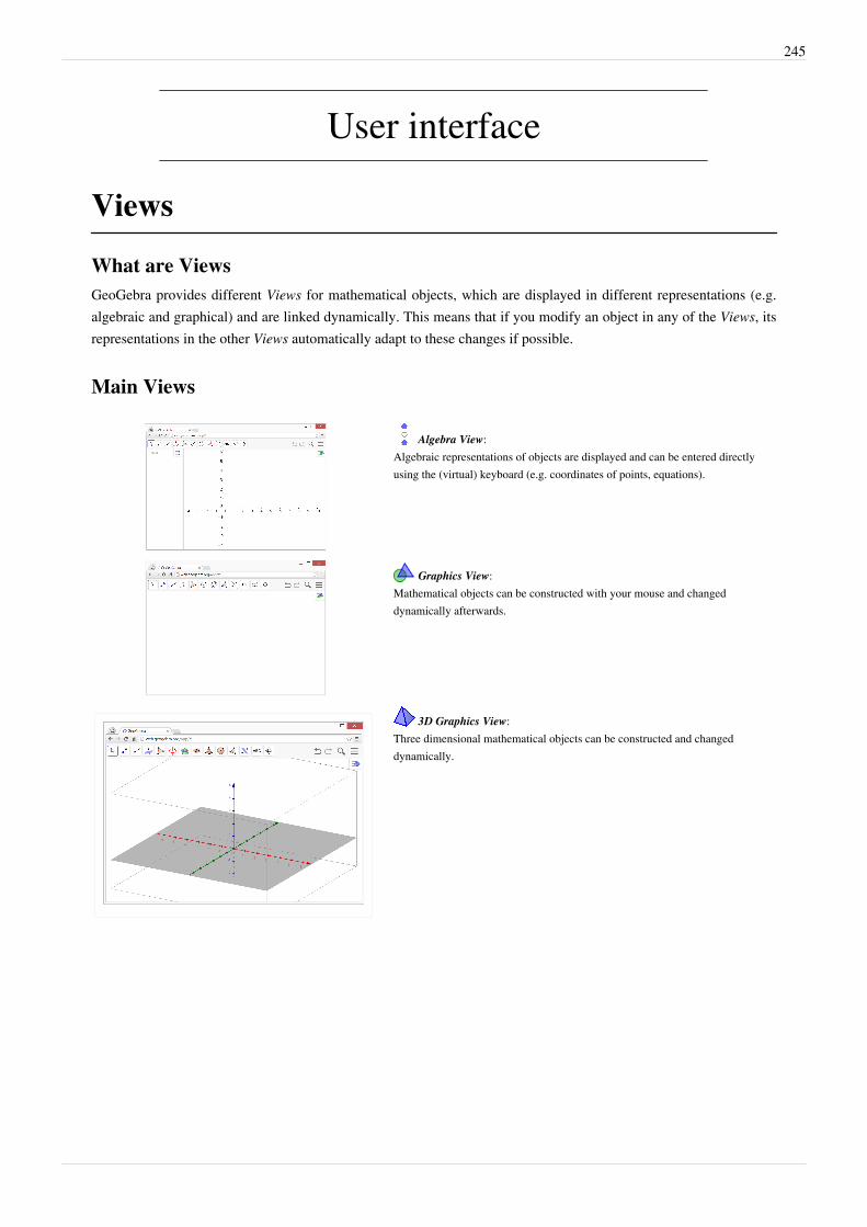
245

User interface

Views

What are ViewsGeoGebra provides different Views for mathematical objects, which are displayed in different representations (e.g.algebraic and graphical) and are linked dynamically. This means that if you modify an object in any of the Views, itsrepresentations in the other Views automatically adapt to these changes if possible.

Main Views

Algebra View:Algebraic representations of objects are displayed and can be entered directlyusing the (virtual) keyboard (e.g. coordinates of points, equations).

Graphics View:Mathematical objects can be constructed with your mouse and changeddynamically afterwards.

3D Graphics View:Three dimensional mathematical objects can be constructed and changeddynamically.

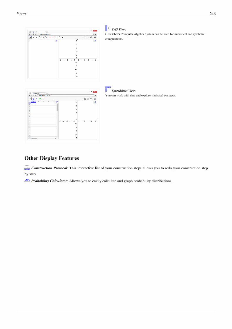
Views 246

CAS View:GeoGebra's Computer Algebra System can be used for numerical and symboliccomputations.

Spreadsheet View:You can work with data and explore statistical concepts.

Other Display Features

Construction Protocol: This interactive list of your construction steps allows you to redo your construction stepby step.

Probability Calculator: Allows you to easily calculate and graph probability distributions.

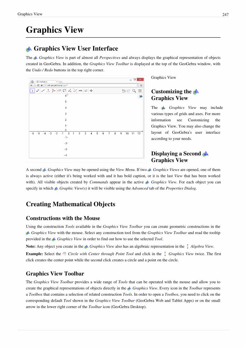
Graphics View 247

Graphics View

Graphics View User InterfaceThe Graphics View is part of almost all Perspectives and always displays the graphical representation of objectscreated in GeoGebra. In addition, the Graphics View Toolbar is displayed at the top of the GeoGebra window, withthe Undo / Redo buttons in the top right corner.

Graphics View

Customizing the Graphics ViewThe Graphics View may includevarious types of grids and axes. For moreinformation see Customizing theGraphics View. You may also change thelayout of GeoGebra’s user interfaceaccording to your needs.

Displaying a Second Graphics View

A second Graphics View may be opened using the View Menu. If two Graphics Views are opened, one of themis always active (either it's being worked with and it has bold caption, or it is the last View that has been workedwith). All visible objects created by Commands appear in the active Graphics View. For each object you canspecify in which Graphic View(s) it will be visible using the Advanced tab of the Properties Dialog.

Creating Mathematical Objects

Constructions with the MouseUsing the construction Tools available in the Graphics View Toolbar you can create geometric constructions in the

Graphics View with the mouse. Select any construction tool from the Graphics View Toolbar and read the tooltipprovided in the Graphics View in order to find out how to use the selected Tool.Note: Any object you create in the Graphics View also has an algebraic representation in the Algebra View.Example: Select the Circle with Center through Point Tool and click in the Graphics View twice. The firstclick creates the center point while the second click creates a circle and a point on the circle.

Graphics View ToolbarThe Graphics View Toolbar provides a wide range of Tools that can be operated with the mouse and allow you tocreate the graphical representations of objects directly in the Graphics View. Every icon in the Toolbar representsa Toolbox that contains a selection of related construction Tools. In order to open a Toolbox, you need to click on thecorresponding default Tool shown in the Graphics View Toolbar (GeoGebra Web and Tablet Apps) or on the smallarrow in the lower right corner of the Toolbar icon (GeoGebra Desktop).

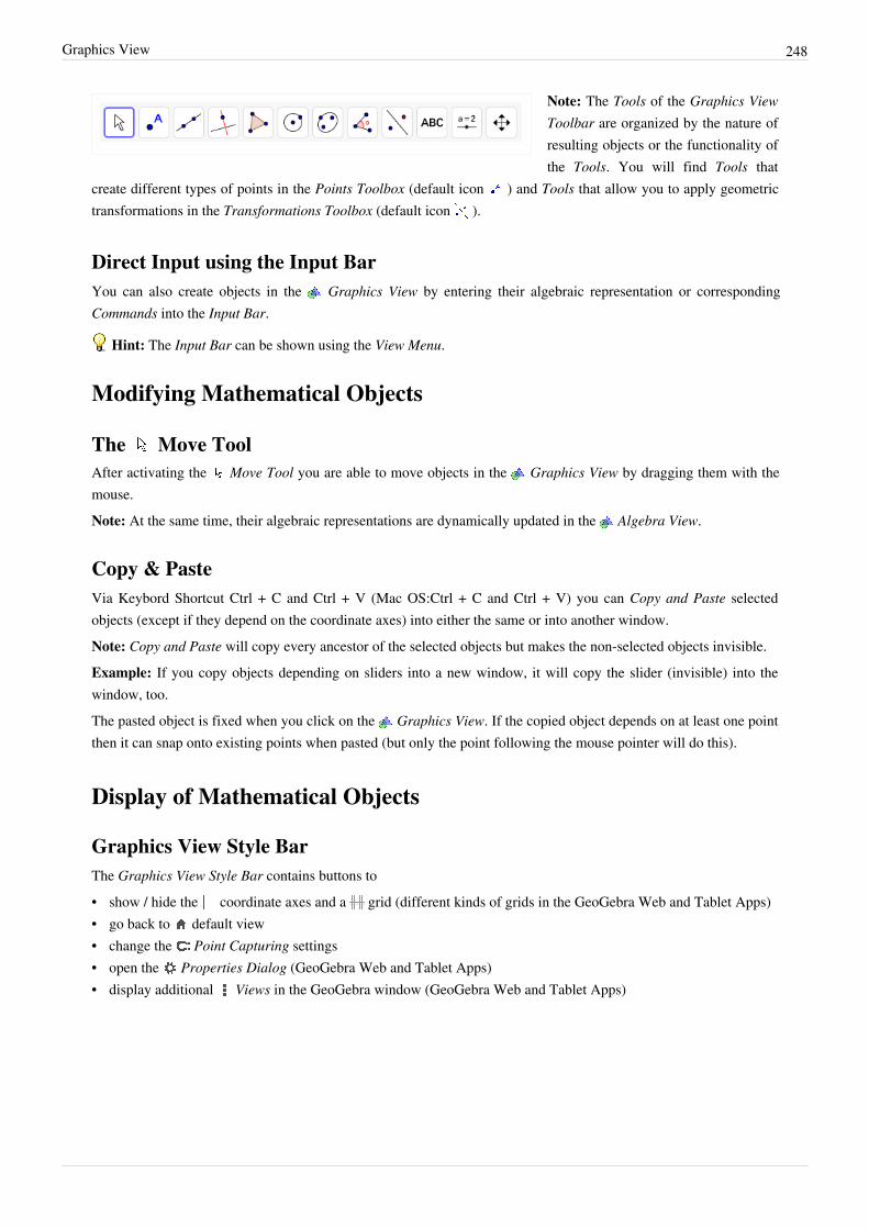
Graphics View 248

Note: The Tools of the Graphics ViewToolbar are organized by the nature ofresulting objects or the functionality ofthe Tools. You will find Tools that

create different types of points in the Points Toolbox (default icon ) and Tools that allow you to apply geometrictransformations in the Transformations Toolbox (default icon ).

Direct Input using the Input BarYou can also create objects in the Graphics View by entering their algebraic representation or correspondingCommands into the Input Bar.

Hint: The Input Bar can be shown using the View Menu.

Modifying Mathematical Objects

The Move ToolAfter activating the Move Tool you are able to move objects in the Graphics View by dragging them with themouse.Note: At the same time, their algebraic representations are dynamically updated in the Algebra View.

Copy & PasteVia Keybord Shortcut Ctrl + C and Ctrl + V (Mac OS:Ctrl + C and Ctrl + V) you can Copy and Paste selectedobjects (except if they depend on the coordinate axes) into either the same or into another window.Note: Copy and Paste will copy every ancestor of the selected objects but makes the non-selected objects invisible.Example: If you copy objects depending on sliders into a new window, it will copy the slider (invisible) into thewindow, too.The pasted object is fixed when you click on the Graphics View. If the copied object depends on at least one pointthen it can snap onto existing points when pasted (but only the point following the mouse pointer will do this).

Display of Mathematical Objects

Graphics View Style BarThe Graphics View Style Bar contains buttons to• show / hide the coordinate axes and a grid (different kinds of grids in the GeoGebra Web and Tablet Apps)• go back to default view• change the Point Capturing settings• open the Properties Dialog (GeoGebra Web and Tablet Apps)• display additional Views in the GeoGebra window (GeoGebra Web and Tablet Apps)

Graphics View 249

Style Bar for Tools and ObjectsDepending on the Tool or object you select, the buttons in the Style Bar adapt to your selection. Please see Style BarOptions for Tools and Objects for more information.

Hiding Mathematical Objects in the Graphics ViewYou may hide objects in the Graphics View by either• using the Show / Hide Object Tool• opening the Context Menu and unchecking Show Object

Customizing the Graphics ViewIn order to adjust the visible part of the drawing pad in the Graphics View, you can drag the drawing pad by using

tool Move Graphics View Tool and use the following ways of zooming:

• You may use the Zoom In Tool and Zoom Out Tool in order to zoom in the Graphics View. Note: Theposition of your click determines the center of zoom.

•• You may use the scroll wheel of your mouse in order to zoom in the Graphics View.•• You may use keyboard shortcuts to zoom in Ctrl + + and to zoom out Ctrl + -.•• After right clicking (Mac OS: Ctrl-click) on an empty spot on the drawing pad a Context Menu appears which

allows you to Zoom.•• You may specify a zoom rectangle by right clicking (Mac OS: Cmd - click) on an empty spot in the Graphics

View and dragging the mouse to the opposite corner of your desired zoom rectangle. Release the mouse button inorder to finish the zoom rectangle, which will then automatically adjust to fill all the space in the Graphics View.

• You may also specify range of x- and y-axis in the Properties Dialog for Graphics view (see below).

Showing and hiding objectsIn the Algebra View, the icon to the left of every object shows its current visibility state (shown or hidden). You maydirectly click on the little marble icon in order to change the visibility status of an object. For more information seevisibility.

Properties of Graphics View (Properties Dialog)Coordinate axes, grid and some other properties can be customized using the Properties Dialog of the GraphicsView. After right clicking (Mac OS: Ctrl-click) on the drawing pad, you can open this dialog window by selectingGraphics... from the appearing Context Menu of the Graphics View.

Customizing the Graphics View 250

Customizing Coordinate Axes and GridTo show or hide the axes and the grid, right click (Mac OS: Ctrl-click) on the drawing pad and select thecorresponding items Axes or Grid from the appearing Context Menu. For further setting you need to open theProperties Dialog.• On tab Basic, you can, for example, change the line style and color of the coordinate axes, and set the the ratio

between the axes . To make sure the axes ratio cannot be changed by any command or user action, you may lockit using the lock icon.

• Clicking on tabs xAxis and yAxis allows you to customize the axes individually, set the distance of the tickmarks,labeling, axes visibility, units and more. If you want the cross of the axes to be at point (a,b), you can set Cross atparameter for xAxis to b and for yAxis to a. Option Stick to edge means that the line remains close to the bottom orleft border of the screen. To draw only the part of the axis to the right or to the top of the axes intersection, youcan select Positive direction only.

• On tab Grid, you can change the color and line style of the coordinate grid, set the distance and ratio for grid linesto a certain value, and the grid visibility. Three types of grid are available: Cartesian, polar and isometric.

Note:Axes scaling is possible in every mode by pressing and holding the Shift-key (PC: also Ctrl-key) whiledragging the axis. Range of the axes may be given dynamically, e.g. in Basic tab you can set X Min to x(A) and YMin to y(A) to ensure the lower left corner of the view remains in point A. In such setting, the view cannot bezoomed.

Showing Navigation BarYou can add Navigation Bar for Construction Steps to the Graphics View by enabling it in Basic Tab of PropertiesDialog. You can also add the Play button to allow animating the construction steps and a button to show theConstruction Protocol.

Miscellaneous settingsThese settings are located in the last part of the Basic tab of Properties Dialog.Background colorAllows you to change background color of the Graphics View.TooltipsAllows you to set the behavior of tooltips in the Graphics View. See article on Tooltips for details.Show mouse coordinatesEnables display of mouse coordinates next to the mouse pointer.

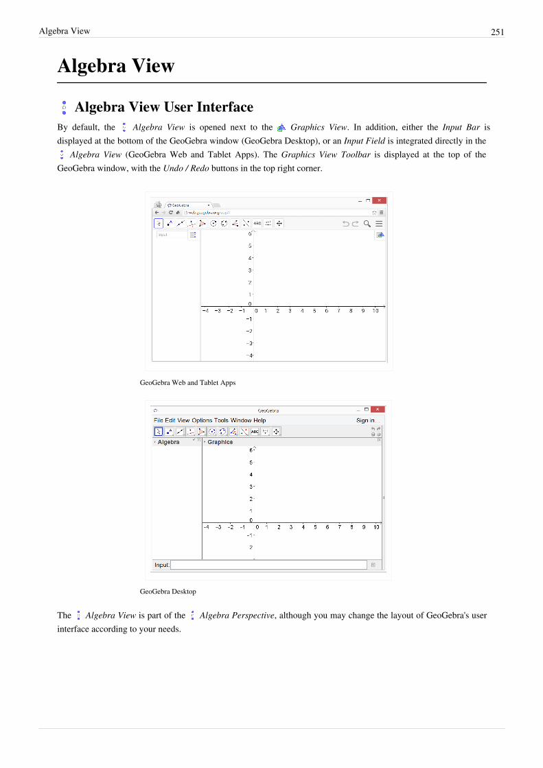
Algebra View 251

Algebra View

Algebra View User InterfaceBy default, the Algebra View is opened next to the Graphics View. In addition, either the Input Bar isdisplayed at the bottom of the GeoGebra window (GeoGebra Desktop), or an Input Field is integrated directly in the

Algebra View (GeoGebra Web and Tablet Apps). The Graphics View Toolbar is displayed at the top of theGeoGebra window, with the Undo / Redo buttons in the top right corner.

GeoGebra Web and Tablet Apps

GeoGebra Desktop

The Algebra View is part of the Algebra Perspective, although you may change the layout of GeoGebra's userinterface according to your needs.

Algebra View 252

Creating Mathematical Objects

Direct InputIn the Algebra View you can directly enter algebraic expressions using the integrated Input Field (GeoGebra Weband Tablet Apps) or the Input Bar at the bottom of the GeoGebra window (GeoGebra Desktop). After hitting theEnter key your algebraic input appears in the Algebra View while its graphical representation is automaticallydisplayed in the Graphics View.Example: The input y = 2 x + 3 gives you the linear equation in the Algebra View and the correspondingline in the Graphics View.

CommandsGeoGebra also offers a wide range of Commands that can be used to create objects in the Algebra View. Just starttyping the name of a Command into the Input Bar or Input Field and GeoGebra will offer you a list of Commandsthat match your input.

ToolsAlthough the Algebra View doesn’t have it’s own Toolbar, you can create Dependent Objects with the mouse.Select a tool from the Graphics View Toolbar and click on any appropriate object in the Algebra View in order tocreate a new Dependent Object.Example: Create two points A and B, whose coordinates are displayed in the Algebra View. Select the LineTool from the Graphics View Toolbar and click on both points in the Algebra View in order to create a linethrough points A and B.

Modifying Mathematical ObjectsYou can modify the algebraic representation of mathematical objects directly in the Algebra View.Activate the Move tool and double click a Free Object in the Algebra View. In the appearing text box you candirectly modify its algebraic representation. After hitting the Enter key, both the algebraic representation in the Algebra View and the graphical representation of the object in the Graphics View will automatically adapt to yourchanges.If you double click on a Dependent Object in the Algebra View, a dialog window appears allowing you toRedefine the object.

Display of Mathematical ObjectsBy default, mathematical objects are organized by Object Types in the Algebra View. In GeoGebra Desktop, youmay use the Style Bar option Sort by in order to re-sort the objects by Dependency, Layer or Construction Order.

Hint: You can collapse or expand each group of objects individually (e.g. all points, all free objects, all objectson a specific layer) by clicking on the plus or minus symbol in front of the group’s name.

Algebra View Style BarThe Algebra View Style Bar provides buttons to• show / hide Auxiliary Objects• sort the list of objects by different criteria

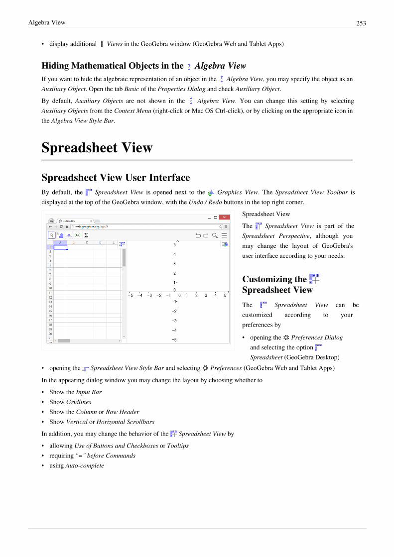
Algebra View 253

• display additional Views in the GeoGebra window (GeoGebra Web and Tablet Apps)

Hiding Mathematical Objects in the Algebra ViewIf you want to hide the algebraic representation of an object in the Algebra View, you may specify the object as anAuxiliary Object. Open the tab Basic of the Properties Dialog and check Auxiliary Object.By default, Auxiliary Objects are not shown in the Algebra View. You can change this setting by selectingAuxiliary Objects from the Context Menu (right-click or Mac OS Ctrl-click), or by clicking on the appropriate icon inthe Algebra View Style Bar.

Spreadsheet View

Spreadsheet View User InterfaceBy default, the Spreadsheet View is opened next to the Graphics View. The Spreadsheet View Toolbar isdisplayed at the top of the GeoGebra window, with the Undo / Redo buttons in the top right corner.

Spreadsheet ViewThe Spreadsheet View is part of theSpreadsheet Perspective, although youmay change the layout of GeoGebra'suser interface according to your needs.

Customizing the Spreadsheet ViewThe Spreadsheet View can becustomized according to yourpreferences by

• opening the Preferences Dialogand selecting the option Spreadsheet (GeoGebra Desktop)

• opening the Spreadsheet View Style Bar and selecting Preferences (GeoGebra Web and Tablet Apps)In the appearing dialog window you may change the layout by choosing whether to• Show the Input Bar• Show Gridlines• Show the Column or Row Header• Show Vertical or Horizontal Scrollbars

In addition, you may change the behavior of the Spreadsheet View by• allowing Use of Buttons and Checkboxes or Tooltips• requiring "=" before Commands• using Auto-complete

Spreadsheet View 254

Creating Mathematical ObjectsIn GeoGebra’s Spreadsheet View every cell has a specific name that allows you to directly address each cell.Example: The cell in column A and row 1 is named A1.Note: These cell names can be used in expressions and Commands in order to address the content of thecorresponding cell.

Direct Input and CommandsIn the Spreadsheet Cells you can enter not only numbers, but all types of General Objects and Geometrical Objectsthat are supported by GeoGebra (e. g., coordinates of points, Functions, Commands).

Relative Cell NamesIf you copy content from one cell to another, by default all references are changed accordingly to the target position.Example: Let A1=1, A2=2. In B1 put (A1, A1). By copying B1 to B2 (either via Ctrl + C, Ctrl + V or bydragging the cell corner) you get (A2, A2) in B2.To prevent this behavior, you can insert $ before the column and/or row of the referenced cell.Note: On Mac OS the Copy & Paste shortcuts are Cmd + C and Cmd + V

Input Data into the Spreadsheet View

Manual Entry, Commands, and TracingBesides manually adding entries into the Spreadsheet View cells, you may use the commands FillColumn,FillRow or FillCells. You can also enter data by using the feature Tracing to Spreadsheet.

Copy Data from the Algebra ViewWith a simple drag and drop operation it is also possible to copy objects from the Algebra View to the Spreadsheet View. If you drag a list, its elements will be pasted horizontally, starting from the cell in which yourelease the left mouse button. Pressing the Shift key while dragging opens a dialog window when the mouse buttonis released, allowing you to choose whether the pasted objects will be Free or Dependent, as well as to choose thevertical placement of the copied objects (check option Transpose).

Copy Data from Other Spreadsheet SoftwareGeoGebra allows you to import data from other spreadsheet software into the Spreadsheet View.• Select and copy the data you want to import. For example, you may use the keyboard shortcut Ctrl + C (Mac OS:

Cmd + C) in order to copy the data to your computer’s clipboard.• Open a GeoGebra window and show the Spreadsheet View.• Click on the spreadsheet cell that should contain the first data value (e.g. cell A1)• Paste the data from your computer’s clipboard into GeoGebra’s Spreadsheet View. For example, you may

select a cell and use the keyboard shortcut Ctrl + V (Mac OS: Cmd + V) in order to paste the data into thehighlighted spreadsheet cell.

.

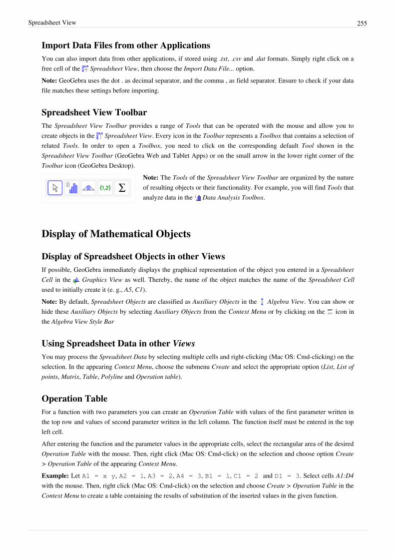
Spreadsheet View 255

Import Data Files from other ApplicationsYou can also import data from other applications, if stored using .txt, .csv and .dat formats. Simply right click on afree cell of the Spreadsheet View, then choose the Import Data File... option.Note: GeoGebra uses the dot . as decimal separator, and the comma , as field separator. Ensure to check if your datafile matches these settings before importing.

Spreadsheet View ToolbarThe Spreadsheet View Toolbar provides a range of Tools that can be operated with the mouse and allow you tocreate objects in the Spreadsheet View. Every icon in the Toolbar represents a Toolbox that contains a selection ofrelated Tools. In order to open a Toolbox, you need to click on the corresponding default Tool shown in theSpreadsheet View Toolbar (GeoGebra Web and Tablet Apps) or on the small arrow in the lower right corner of theToolbar icon (GeoGebra Desktop).

Note: The Tools of the Spreadsheet View Toolbar are organized by the natureof resulting objects or their functionality. For example, you will find Tools thatanalyze data in the Data Analysis Toolbox.

Display of Mathematical Objects

Display of Spreadsheet Objects in other ViewsIf possible, GeoGebra immediately displays the graphical representation of the object you entered in a SpreadsheetCell in the Graphics View as well. Thereby, the name of the object matches the name of the Spreadsheet Cellused to initially create it (e. g., A5, C1).Note: By default, Spreadsheet Objects are classified as Auxiliary Objects in the Algebra View. You can show orhide these Auxiliary Objects by selecting Auxiliary Objects from the Context Menu or by clicking on the icon inthe Algebra View Style Bar

Using Spreadsheet Data in other ViewsYou may process the Spreadsheet Data by selecting multiple cells and right-clicking (Mac OS: Cmd-clicking) on theselection. In the appearing Context Menu, choose the submenu Create and select the appropriate option (List, List ofpoints, Matrix, Table, Polyline and Operation table).

Operation TableFor a function with two parameters you can create an Operation Table with values of the first parameter written inthe top row and values of second parameter written in the left column. The function itself must be entered in the topleft cell.After entering the function and the parameter values in the appropriate cells, select the rectangular area of the desiredOperation Table with the mouse. Then, right click (Mac OS: Cmd-click) on the selection and choose option Create> Operation Table of the appearing Context Menu.Example: Let A1 = x y, A2 = 1, A3 = 2, A4 = 3, B1 = 1, C1 = 2 and D1 = 3. Select cells A1:D4with the mouse. Then, right click (Mac OS: Cmd-click) on the selection and choose Create > Operation Table in theContext Menu to create a table containing the results of substitution of the inserted values in the given function.

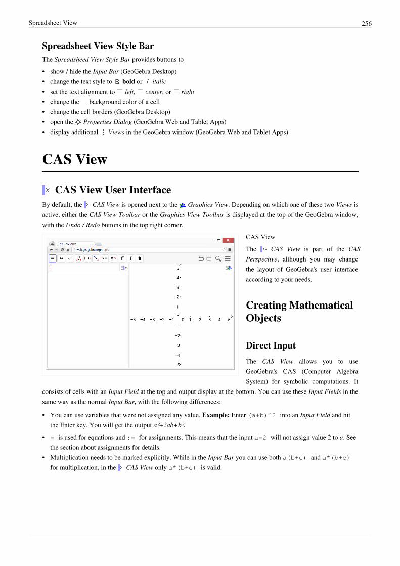
Spreadsheet View 256

Spreadsheet View Style BarThe Spreadsheed View Style Bar provides buttons to• show / hide the Input Bar (GeoGebra Desktop)• change the text style to bold or italic• set the text alignment to left, center, or right• change the background color of a cell•• change the cell borders (GeoGebra Desktop)• open the Properties Dialog (GeoGebra Web and Tablet Apps)• display additional Views in the GeoGebra window (GeoGebra Web and Tablet Apps)

CAS View

CAS View User InterfaceBy default, the CAS View is opened next to the Graphics View. Depending on which one of these two Views isactive, either the CAS View Toolbar or the Graphics View Toolbar is displayed at the top of the GeoGebra window,with the Undo / Redo buttons in the top right corner.

CAS ViewThe CAS View is part of the CASPerspective, although you may changethe layout of GeoGebra's user interfaceaccording to your needs.

Creating MathematicalObjects

Direct Input

The CAS View allows you to useGeoGebra's CAS (Computer AlgebraSystem) for symbolic computations. It

consists of cells with an Input Field at the top and output display at the bottom. You can use these Input Fields in thesame way as the normal Input Bar, with the following differences:

• You can use variables that were not assigned any value. Example: Enter (a+b)^2 into an Input Field and hitthe Enter key. You will get the output a²+2ab+b².

• = is used for equations and := for assignments. This means that the input a=2 will not assign value 2 to a. Seethe section about assignments for details.

• Multiplication needs to be marked explicitly. While in the Input Bar you can use both a(b+c) and a*(b+c)for multiplication, in the CAS View only a*(b+c) is valid.

CAS View 257

Keyboard Shortcuts for Direct InputIn the CAS View the following keyboard shortcuts help you to evaluate or check your input.Note: Instead of using these keyboard shortcuts, you may also use the corresponding Tools of the CAS ViewToolbar.•• Enter: Evaluates you input• Ctrl + Enter: Evaluates your input numerically Example: sqrt(2) yields 1.41

• Alt + Enter: Checks your input but does not evaluate it. Example: b + b stays as b + b.Note: Assignments are always evaluated, e.g. a := 5In the CAS View the following keyboard shortcuts help you to reuse previous input or output in a new row if youenter them into an empty Input Field:•• Space bar: Inserts the previous output into the new row.• ): Inserts the previous output in parentheses.• =: Inserts the previous input into the new row.Note: You may suppress any output with a semicolon at the end of your input, e.g. a := 5;.

Variable Assignments and Connection with other ViewsYou may use the := notation for assignments, e.g. b := 5, a(n) := 2n + 3.• Free up a name: Use Delete[b] in order to free up a variable name again.• Redefine a variable or function: You may redefine a variable or function, but you must do so in the same cell,

otherwise it will be treated as a new variable and automatically renamed.Variables and functions are always shared between the CAS View and the other Views if possible. For example:• If you define b:=5 in the CAS View, then you can use b in all the other Views of GeoGebra.• If you define a function f(x)=x^2 in another View, you can also use this function in the CAS View.Note:

The output will always be just the expression after the :=, e.g. if you type b:=5 the output will be 5. Please alsonote, that for clarification actually b := 5 will be displayed.

Equations• You may write equations using the simple Equals sign, e.g. 3x + 5 = 7.• Arithmetic operations: You can perform arithmetic operations on equations, which is useful for manual equation

solving. Example: (3x + 5 = 7) - 5 subtracts 5 from both sides of the equation.• Extracting one Side: You may extract either the left or right side of an equation by using the commandsLeftSide[] and RightSide[]. Example: LeftSide[3x + 5 = 7] returns 3 x + 5 andRightSide[3x + 5 = 7] returns 7

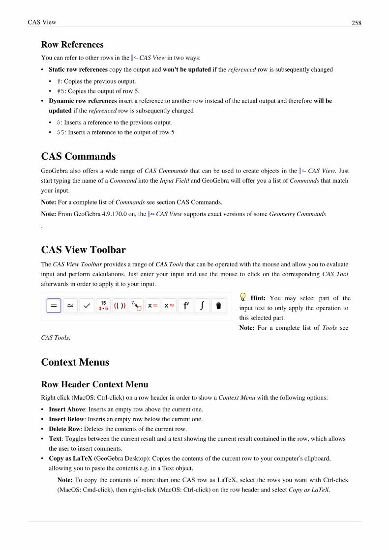
CAS View 258

Row ReferencesYou can refer to other rows in the CAS View in two ways:• Static row references copy the output and won't be updated if the referenced row is subsequently changed

• #: Copies the previous output.• #5: Copies the output of row 5.

• Dynamic row references insert a reference to another row instead of the actual output and therefore will beupdated if the referenced row is subsequently changed• $: Inserts a reference to the previous output.• $5: Inserts a reference to the output of row 5

CAS CommandsGeoGebra also offers a wide range of CAS Commands that can be used to create objects in the CAS View. Juststart typing the name of a Command into the Input Field and GeoGebra will offer you a list of Commands that matchyour input.Note: For a complete list of Commands see section CAS Commands.Note: From GeoGebra 4.9.170.0 on, the CAS View supports exact versions of some Geometry Commands

.

CAS View ToolbarThe CAS View Toolbar provides a range of CAS Tools that can be operated with the mouse and allow you to evaluateinput and perform calculations. Just enter your input and use the mouse to click on the corresponding CAS Toolafterwards in order to apply it to your input.

Hint: You may select part of theinput text to only apply the operation tothis selected part.Note: For a complete list of Tools see

CAS Tools.

Context Menus

Row Header Context MenuRight click (MacOS: Ctrl-click) on a row header in order to show a Context Menu with the following options:• Insert Above: Inserts an empty row above the current one.• Insert Below: Inserts an empty row below the current one.• Delete Row: Deletes the contents of the current row.• Text: Toggles between the current result and a text showing the current result contained in the row, which allows

the user to insert comments.• Copy as LaTeX (GeoGebra Desktop): Copies the contents of the current row to your computer’s clipboard,

allowing you to paste the contents e.g. in a Text object.Note: To copy the contents of more than one CAS row as LaTeX, select the rows you want with Ctrl-click(MacOS: Cmd-click), then right-click (MacOS: Ctrl-click) on the row header and select Copy as LaTeX.

CAS View 259

Cell Context MenuIn GeoGebra Desktop, right click (MacOS: Ctrl-click) on a CAS output cell in order to show a Context Menu withthe following options:• Copy: Copies the cell contents to the your computer’s clipboard. Then, right click on a new cell in order to show

the Paste option.• Copy as LaTeX: Copies the cell contents in LaTeX format to the your computer’s clipboard, so it can be pasted

into a Text object or a LaTeX editor.• Copy as LibreOffice Formula: Copies the cell contents in LibreOffice formula format to your computer’s

clipboard, so it can be pasted in a word processing document.• Copy as Image: Copies the cell contents in PNG format to your computer’s clipboard, so it can be pasted into an

Image object or in a word processing document.

Display of Mathematical Objects

CAS View Style BarThe CAS View Style Bar provides buttons to• change the text style ( bold and italics) and color• display a virtual keyboard (GeoGebra Desktop)• display additional Views in the GeoGebra window (GeoGebra Web and Tablet Apps)

Showing CAS Objects in the Graphics ViewIn the CAS View, the icon to the left of every row shows the current visibility state (shown or hidden) of theobject defined in it (when possible). You may directly click on the little Show / Hide Object icon in order tochange the visibility status of the object in the Graphics View.

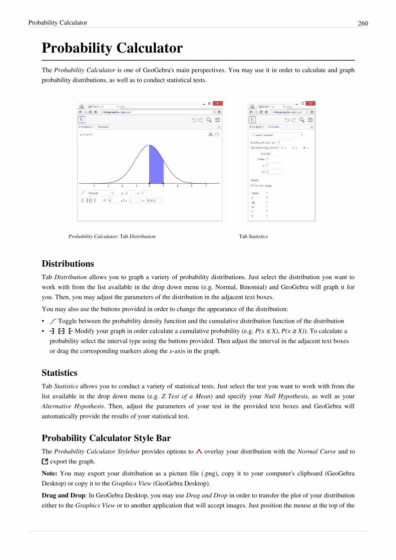
Probability Calculator 260

Probability CalculatorThe Probability Calculator is one of GeoGebra's main perspectives. You may use it in order to calculate and graphprobability distributions, as well as to conduct statistical tests.

Probability Calculator: Tab Distribution Tab Statistics

DistributionsTab Distribution allows you to graph a variety of probability distributions. Just select the distribution you want towork with from the list available in the drop down menu (e.g. Normal, Binomial) and GeoGebra will graph it foryou. Then, you may adjust the parameters of the distribution in the adjacent text boxes.You may also use the buttons provided in order to change the appearance of the distribution:• Toggle between the probability density function and the cumulative distribution function of the distribution• Modify your graph in order calculate a cumulative probability (e.g. P(x ≤ X), P(x ≥ X)). To calculate a

probability select the interval type using the buttons provided. Then adjust the interval in the adjacent text boxesor drag the corresponding markers along the x-axis in the graph.

StatisticsTab Statistics allows you to conduct a variety of statistical tests. Just select the test you want to work with from thelist available in the drop down menu (e.g. Z Test of a Mean) and specify your Null Hypothesis, as well as yourAlternative Hypothesis. Then, adjust the parameters of your test in the provided text boxes and GeoGebra willautomatically provide the results of your statistical test.

Probability Calculator Style BarThe Probability Calculator Stylebar provides options to overlay your distribution with the Normal Curve and to

export the graph.Note: You may export your distribution as a picture file (.png), copy it to your computer's clipboard (GeoGebraDesktop) or copy it to the Graphics View (GeoGebra Desktop).Drag and Drop: In GeoGebra Desktop, you may use Drag and Drop in order to transfer the plot of your distribution either to the Graphics View or to another application that will accept images. Just position the mouse at the top of the

Probability Calculator 261

Probability Calculator screen and the cursor will change to a hand cursor. This new cursor allows you to drag theplot into Graphics View 1 or 2 to create a new plot or to drag an image of the plot into another application.

Construction ProtocolYou can access the interactive Construction Protocol by selecting the Construction Protocol option in the Viewmenu. The Construction Protocol is a table that shows all construction steps, allowing you to redo a construction stepby step. To show the Navigation Bar at the bottom of the GeoGebra window, right click in the Graphics View, thenselect the Navigation bar option in the context menu displayed.

Navigating and Modifying the Construction ProtocolYou may use the keyboard to navigate in the Construction Protocol:• Press the ↑ up arrow of your keyboard to go to the previous construction step.• Press the ↓ down arrow of you keyboard to go to the next construction step.•• Press the Home key to return to the beginning of the Construction Protocol.•• Press the End key to move to the end of the Construction Protocol.•• Press the Delete key to delete the selected construction step.

Note: This may also affect other objects that depend on the selected object/construction step.You may also use the mouse in order to navigate in the Construction Protocol:•• Double click a row to select a construction step.•• Double click the header of any column to go to the beginning of the Construction Protocol.•• Drag and drop a row to move a construction step to another position in the Construction Protocol.

Note: This is not always possible due to the dependencies between different objects.•• Right click on a row to open the context menu related to the currently selected object.Note: You can insert construction steps at any position. Select the construction step below the one you would like toinsert a new construction step. Leave the Construction Protocol window open while you create a new object. Thisnew construction step is immediately inserted into the selected position of the Construction Protocol.Select the options listed when you click the first icon of the Construction Protocol toolbar, to decide whichinformations related to the construction will be shown. The Breakpoint option allows you to define certainconstruction steps as breakpoints, i.e. group several objects together. When navigating through your constructionusing the Navigation Bar, selected groups of objects are shown at the same time.

Exporting the Construction Protocol as a WebpageGeoGebra allows you to export the Construction Protocol as a Webpage. Open the Construction Protocol using therelated option in the View menu, then click the third icon of the Contruction Protocol's toolbar (Export as Webpage).In the export window of the Construction Protocol you can enter Title, Author, and a Date for the construction andchoose whether or not you want to include a picture of the Graphics View and the Algebra View. In addition, youcan also choose to export a Colorful Construction Protocol. This means that objects in the Construction Protocolwill match the color of the corresponding objects in the construction.

Note: The exported HTML file can be viewed with any Internet browser (e. g. Firefox, Internet Explorer) andedited with many text processing systems (e. g. OpenOffice Writer).

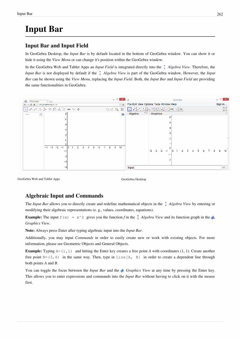
Input Bar 262

Input Bar

Input Bar and Input FieldIn GeoGebra Desktop, the Input Bar is by default located in the bottom of GeoGebra window. You can show it orhide it using the View Menu or can change it's position within the GeoGebra window.In the GeoGebra Web and Tablet Apps an Input Field is integrated directly into the Algebra View. Therefore, theInput Bar is not displayed by default if the Algebra View is part of the GeoGebra window. However, the InputBar can be shown using the View Menu, replacing the Input Field. Both, the Input Bar and Input Field are providingthe same functionalities in GeoGebra.

GeoGebra Web and Tablet Apps GeoGebra Desktop

Algebraic Input and CommandsThe Input Bar allows you to directly create and redefine mathematical objects in the Algebra View by entering ormodifying their algebraic representations (e. g., values, coordinates, equations).Example: The input f(x) = x^2 gives you the function f in the Algebra View and its function graph in the Graphics View.Note: Always press Enter after typing algebraic input into the Input Bar.Additionally, you may input Commands in order to easily create new or work with existing objects. For moreinformation, please see Geometric Objects and General Objects.Example: Typing A=(1,1) and hitting the Enter key creates a free point A with coordinates (1, 1). Create anotherfree point B=(3,4) in the same way. Then, type in Line[A, B] in order to create a dependent line throughboth points A and B.You can toggle the focus between the Input Bar and the Graphics View at any time by pressing the Enter key.This allows you to enter expressions and commands into the Input Bar without having to click on it with the mousefirst.

Input Bar 263

Displaying Input HistoryAfter placing the cursor in the Input Bar you can use the ↑ up and ↓ down arrow keys of your keyboard in order tonavigate through prior input step by step. Hit the Enter key in order to transfer the selected prior input back into theInput Bar.

Insert Name, Value, or Definition of an Object into the Input BarInsert the name of an object: Activate the  Move Tool and select the object whose name you want to insert intothe Input Bar. Then, press F5 on your keyboard.Note: The name of the object is appended to any expression you typed into the Input Bar before pressing F5.Insert the value of an object: To insert an object’s value (e. g., coordinates of a point (1, 3), equation 3x – 5y= 12) into the Input Bar, select the Move Tool and click on the object whose value you want to insert into theInput Bar. Then, press F4 on your keyboard.Note: The value of the object is appended to any expression you typed into the Input Bar before pressing F4.Insert the definition of an object: There are two ways of inserting an object’s definition (e. g., A = (4, 2), c= Circle[A, B]) into the Input Bar.• Alt + click on the object to insert the object’s definition and delete whatever input might have been in the Input

Bar before.• Activate the Move Tool and select the object whose definition you want to insert into the Input Bar. Then,

press F3 on your keyboard.Note: The definition of the object replaces any expression you typed into the Input Bar before pressing F3.

MenubarThe Menubar is always situated in the top part of GeoGebra window. For applets it can be switched on and offduring export. It contains following menus:•• File Menu•• Edit Menu•• View Menu•• Options Menu•• Tools Menu•• Window Menu•• Help Menu

Toolbar 264

ToolbarBy default the Toolbar is located at the top of the GeoGebra window or right below the Menubar (GeoGebraDesktop). The Toolbar is divided into Toolboxes, containing one or more related Tools.

Graphics View Toolbar

Tool HelpIf you select a Tool, a tooltip appearsexplaining how to use this Tool.

Note: When you click on the tooltip inthe GeoGebra Web and Tablet Apps,a web page providing help for theselected tool opens in your browser.

If you are using GeoGebra Desktop,click on the Help button in the upperright corner of the GeoGebra window inorder to show the Tool Help Dialog and

get more information about how to use the selected Tool. Furthermore, you can access the online help by clicking onthe button Show Online Help provided in the Tool Help Dialog. In addition, you can display the Toolbar Help to theright of the Toolbar by using the Layout option in the View Menu and checking Show Toolbar Help.

Different Toolbars for Different ViewsEach View except the Algebra View has its own Toolbar, providing Tools specific for the View you are working with.

Graphics View Toolbar

3D Graphics View Toolbar

CAS View Toolbar

Spreadsheet View Toolbar

Once you start using another View within the GeoGebra window, the Toolbar changes automatically. If you openanother View in a separate window, it will have its Toolbar attached.

Toolbar 265

Customizing the Toolbar

Creating a Custom ToolbarThe different Toolbars can be customized by selecting Customize Toolbar… from the Tools Menu.• From the drop-down list select the Toolbar of the View you want to edit.• To remove a Tool or entire Toolbox from the custom Toolbar, select it in the list on the left hand side of the

appearing dialog window and click the button Remove >.• To add a Tool to your custom Toolbar, select it in the right list and click the button < Insert.• To add a Tool to a new Toolbox, select a Toolbox in the left list and the Tool you want to insert in the right list.

Then, click < Insert. Your Tool is inserted as part of a new Toolbox below the selected Toolbox.• To add a Tool to an existing Toolbox, open the Toolbox in the left list and select the Tool above the desired

position of the new Tool. Then, select the Tool from the right list and click < Insert.• To move a Tool from one Toolbox to another, you need to remove the Tool first and then add it to the other

Toolbox.Note: You can restore the default Toolbar by clicking on the button Restore Default Toolbar in the left lower cornerof the dialog window.

Changing the Position of the ToolbarIn GeoGebra Desktop, you can change the position of the Toolbar using the Layout option in the View Menu.

Changing the Toolbar in a GeoGebra AppletThe appearance of the Toolbar in a Dynamic Worksheets can be set using the customToolBar parameter.

Navigation Bar 266

Navigation BarGeoGebra offers a Navigation Bar that allows you to navigate through the construction steps of your GeoGebra file.The Navigation Bar is shown at the bottom of the Graphics View.To display it: Right click (Mac OS: Ctrl-click) on an empty spot on the drawing pad, then select the optionNavigation Bar in the appearing context menu .The Navigation Bar provides a set of navigation buttons, and displays the number of construction steps (e. g. 2 / 7means that the second step of a total of 7 construction steps is currently displayed):• button: go back to step 1• button: go back step by step• button: go forward step by step• button: go to the last step• Play: automatically play the construction, step by step

Note: You may change the speed of this automatic play feature using the text box to the right of the Play button.

• Pause: pause the automatic play featureNote: This button only appears after clicking on the Play button.

• button: This button opens the Construction ProtocolNote: This button only appears if option 'Button to open construction protocol' is enabled.

File Menu

New WindowKeyboard shortcut: Ctrl + N (MacOS: Cmd + N)

This menu item opens a new GeoGebra window that uses the default settings of the GeoGebra user interface.Note: If you change and save some of these settings, the new GeoGebra window will open using your customizedsettings.

NewThis menu item opens a new and empty user interface in the same GeoGebra window. You are asked if youwould like to save the existing construction before opening the new user interface.

Note: The new user interface adopts the settings used for the prior construction. For example, if the coordinate axeswere hidden before selecting the menu item New, the axes will be hidden in the new user interface as well.

File Menu 267

Open...Keyboard shortcut: Ctrl + O (MacOS: Cmd + O)This menu item allows you to open a GeoGebra worksheet (file name extension GGB), Style Template File(file name extension GGB), GeoGebra tool (file name extension GGT) or dynamic worksheet (HTM or HTMLfile produced by GeoGebra) that is saved on your computer.It also allows you to open and insert a GeoGebra file in another one.

Note: In order to open a GeoGebra file you can also drag it with the mouse to the GeoGebra window and drop itthere.

Open Webpage...This menu item allows you to open a Webpage containing a GeoGebra applet, just entering the Webpageaddress in the appearing dialog.

Open Recent (submenu)Lists up to eight recently opened files.

SaveKeyboard shortcut: Ctrl + S (MacOS: Cmd + S)This menu item allows you to save your current construction as a GeoGebra file (file name extension GGB) onyour computer.

Note: If the file was saved before, this menu item overwrites the old file by using the same file name.

Save as...This menu item allows you to save your current construction as a GeoGebra file (file name extension GGB).You will be asked to enter a new name for your GeoGebra file before it is saved on your computer.

ShareLets you upload your worksheet directly to GeoGebraTube [1], see also Dynamic Worksheet as Webpage (html)... .

Export (submenu)Offers several export possibilities:

• Dynamic Worksheet as Webpage (html)...• Graphics View as Picture (png, eps)…• Graphics View to Clipboard• ...and others

File Menu 268

Print PreviewKeyboard shortcut: Ctrl + P (MacOS: Cmd + P)This menu item opens the Print Preview window for the Graphics View. You may specify Title, Author, Dateand the Scale of your printout (in cm).

Note: Press the Enter-key after you made a change in order to update the preview of your printout.

CloseKeyboard shortcut: Alt + F4 (MacOS: Cmd + W)This menu item closes the GeoGebra window. If you didn’t save your construction prior to selecting Close,you are asked if you would like to do so.

Edit Menu

UndoKeyboard shortcut: Ctrl + Z (MacOS: Cmd + Z)This menu item allows you to undo your activities step by step.

Note: You can also use the Undo button to the right of the Toolbar.

RedoKeyboard shortcut: Ctrl + Y (MacOS: Cmd + Shift + Z)This menu item allows you to redo your activities step by step.

Note: You can also use the Redo button to the right of the Toolbar.

CopyKeyboard shortcut: Ctrl + C (MacOS: Cmd + C)Copies the currently selected objects to GeoGebra's internal clipboard

PasteKeyboard shortcut: Ctrl + V (MacOS: Cmd + V)Pastes the objects from GeoGebra's internal clipboard into the currently selected Graphics View. You mustthen click the mouse where you would like to put them (if you move the mouse near an existing point it will"lock" onto it).

Edit Menu 269

Object Properties…Keyboard shortcut: Ctrl + E (MacOS: Cmd + E)This menu item opens the Properties Dialog which allows you to modify the properties of all objects used inthe GeoGebra file.

Select AllKeyboard shortcut: Ctrl + A (MacOS: Cmd + A)This menu item allows you to select all objects used in your construction.

Select Current LayerKeyboard shortcut: Ctrl + L (MacOS: Cmd + L)This menu item allows you to select all objects that are on the same layer as a selected object.

Note: You need to select one object that lies on the desired layer prior to using this menu item.

Select DescendantsKeyboard shortcut: Ctrl + Shift + J (MacOS: Cmd + Shift + J)This menu item allows you to select all objects that depend on the selected object.

Note: You need to select the parent object prior to using this menu item.

Select AncestorsKeyboard shortcut: Ctrl + J (MacOS: Cmd + J)This menu item allows you to select all objects that are ancestors of the selected object, meaning all objects theselected one depends on.

Note: You need to select the dependent object prior to using this menu item.

Invert SelectionKeyboard shortcut: Ctrl + I (MacOS: Cmd + I)

Deselects selected objects and vice versa.

Show / Hide ObjectsKeyboard shortcut: Ctrl + G (MacOS: Cmd + G)

Toggles the visibity of selected objects.

Show / Hide LabelsKeyboard shortcut: Ctrl + Shift + G (MacOS: Cmd + Shift + G)

Shows hidden labels for selected objects and hides the shown ones.

Graphics View to ClipboardKeyboard shortcut: Ctrl + Shift + C (MacOS: Cmd + Shift + C)

Edit Menu 270

This menu item copies the Graphics View to your computer’s clipboard. Afterwards, you can easily paste thispicture into other documents (e. g., word processing document).

DeleteKeyboard shortcut: DeleteThis menu items allows you to delete selected objects and their dependent objects.

Note: You need to select the objects you want to delete first (e. g., use a selection rectangle).

View Menu

AlgebraKeyboard shortcut: Ctrl + Shift + A (MacOS: Cmd + Shift + A)This menu item allows you to show or hide the Algebra View.

SpreadsheetKeyboard shortcut: Ctrl + Shift + S (MacOS: Cmd + Shift + S)This menu item allows you to show or hide the Spreadsheet View.

CASKeyboard shortcut: Ctrl + Shift + K (MacOS: Cmd + Shift + K)This menu item allows you to show or hide the CAS View.

GraphicsKeyboard shortcut: Ctrl + Shift + 1 (MacOS: Cmd + Shift + 1)This menu item allows you to show or hide the Graphics View.

Graphics 2Keyboard shortcut: Ctrl + Shift + 2 (MacOS: Cmd + Shift + 2)This menu item allows you to show or hide a second Graphic View.

Graphique 3DKeyboard shortcut: Ctrl + Maj + 2 (MacOS: Cmd + Maj + 3)

This menu item allows you to show or hide a second Graphic View 3D.

View Menu 271

Construction Protocol…This menu item opens the Construction Protocol dialog.

KeyboardThis menu item allows you to show or hide the Virtual Keyboard, that you can use with a mouse, and containsthe standard keyboard characters, as well as the most used mathematical symbols and operators.

Input BarThis menu item allows you to show or hide the Input Bar and the Command List at the bottom of theGeoGebra window.

Layout...This menu opens the dialog in which you can configure:

Input Bar and the list of commandsThe toolbarThe menu and style barsThe sidebar

Refresh ViewsKeyboard shortcut: Ctrl + F (MacOS: Cmd + F)This menu item allows you to repaint all views on screen.

Note: You can use this menu item to delete any traces of points or lines in the Graphics View.

Recompute all objectsKeyboard shortcut: Ctrl + R (MacOS: Cmd + R)

or F9This menu item recomputes all objects used in your GeoGebra file.

Note: You can use this menu item to create new random numbers if you used any in your GeoGebrafile.

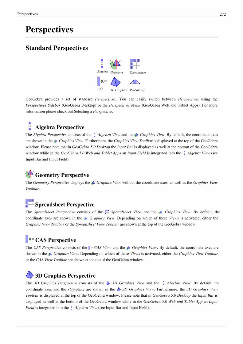
Perspectives 272

Perspectives

Standard Perspectives

Algebra Geometry Spreadsheet

CAS 3D Graphics Probability

GeoGebra provides a set of standard Perspectives. You can easily switch between Perspectives using thePerspectives Sidebar (GeoGebra Desktop) or the Perspectives Menu (GeoGebra Web and Tablet Apps). For moreinformation please check out Selecting a Perspective.

Algebra PerspectiveThe Algebra Perspective consists of the Algebra View and the Graphics View. By default, the coordinate axesare shown in the Graphics View. Furthermore, the Graphics View Toolbar is displayed at the top of the GeoGebrawindow. Please note that in GeoGebra 5.0 Desktop the Input Bar is displayed as well at the bottom of the GeoGebrawindow while in the GeoGebra 5.0 Web and Tablet Apps an Input Field is integrated into the Algebra View (seeInput Bar and Input Field).

Geometry PerspectiveThe Geometry Perspective displays the Graphics View without the coordinate axes, as well as the Graphics ViewToolbar.

Spreadsheet PerspectiveThe Spreadsheet Perspective consists of the Spreadsheet View and the Graphics View. By default, thecoordinate axes are shown in the Graphics View. Depending on which of these Views is activated, either theGraphics View Toolbar or the Spreadsheet View Toolbar are shown at the top of the GeoGebra window.

CAS PerspectiveThe CAS Perspective consists of the CAS View and the Graphics View. By default, the coordinate axes areshown in the Graphics View. Depending on which of these Views is activated, either the Graphics View Toolbaror the CAS View Toolbar are shown at the top of the GeoGebra window.

3D Graphics PerspectiveThe 3D Graphics Perspective consists of the 3D Graphics View and the Algebra View. By default, thecoordinate axes and the xOy-plane are shown in the 3D Graphics View. Furthermore, the 3D Graphics ViewToolbar is displayed at the top of the GeoGebra window. Please note that in GeoGebra 5.0 Desktop the Input Bar isdisplayed as well at the bottom of the GeoGebra window while in the GeoGebra 5.0 Web and Tablet App an InputField is integrated into the Algebra View (see Input Bar and Input Field).

Perspectives 273

Probability PerspectiveThe Probability Perspective shows the Probability Calculator, which allows you to easily calculate and graphprobability distributions.

Customized PerspectivesGeoGebra allows you to customize its user interface according to the mathematical topic you want to work with.You can add additional Views or other user interface components (e.g. Input Bar, second Graphics View) to thestandard Perspectives by using the View Menu or the corresponding Views Button in the Style Bar (GeoGebraWeb and Tablet Apps). Furthermore, you can change the position of some of these elements using the Layoutoption in the Preferences Dialog in GeoGebra Desktop or the Drag View Button in the GeoGebraWeb App.For more information please see Customizing the Layout of the User Interface.

Options MenuGlobal options may be changed in the menu Options.Note: To change object settings, please use the Context Menu and Properties Dialog.

Algebra DescriptionsYou can set how will objects be represented in Algebra View with this item. There are three possibilities:

• Value: show current value of the object.• Definition: show user-friendly description of the object, e.g. "Intersection of a and b."• Command: show the command that was used to create the object, e.g. "Intersect[a,b]".

RoundingThis menu item allows you to set the number of decimal places or significant figures displayed on screen.

LabelingYou can specify whether the label of a newly created object should be shown or not. You can choose between thesettings All New Objects, No New Objects, New Points Only, and Automatic.Note: The setting Automatic shows the labels of newly created objects if the Algebra View is shown.

Font SizeThis menu item determines the font size for labels and text in points (pt).Note: If you are using GeoGebra as a presentation tool, increasing the font size makes it easier for your audience toread text, labels, and algebraic input you are using.

Options Menu 274

LanguageGeoGebra is multilingual and allows you to change the current language setting. This affects all input includingcommand names and all output.Note: No matter which language was selected, the globe icon will lead you back to the Language menu. Alllanguage names are always displayed in English.

AdvancedThis menu item opens the Advanced section of the Preferences Dialog.Note: You can also open this dialog window by right clicking (Mac OS: Ctrl‐click) on the Graphics View orSpreadsheet View and selecting Graphics ... and Spreadsheet Options respectively.

Save SettingsGeoGebra remembers your favorite settings (e. g., settings in the Options menu, current Toolbar and Graphics Viewsettings) if you select Save settings in the Options menu.

Restore Default SettingsYou can restore the default settings of GeoGebra using this menu item.

Tools Menu

Create New Tool…Based on an existing construction you can create your own tools in GeoGebra. After preparing the construction ofyour tool, choose Create new tool in the Tools Menu. In the appearing dialog you can specify the output and inputobjects of your tool and choose names for the Toolbar icon and corresponding command.Note: Your tool can be used both with the mouse and as a command in the Input Bar. All tools are automaticallysaved in your GGB construction file.

Manage Tools…Using the Manage tools dialog you can delete a tool or modify its name and icon. You can also save selected tools toa GeoGebra Tools File (GGT). This file can be used later on (File menu, Open) to load the tools into anotherconstruction.Note: Opening a GGT file doesn’t change your current construction, but opening a GGB file does.

Customize Toolbar…Opens Customize Toolbar Dialog.

Window Menu 275

Window Menu

New WindowKeyboard shortcut: Ctrl + N (MacOS: Cmd + N)

See File Menu > New Window.

List of GeoGebra windowsIf you have more than one GeoGebra window open, this menu item allows you to switch between these differentwindows.

Note: This might be helpful when you are using GeoGebra as a presentation tool and want to have severalGeoGebra files open at the same time as well as to toggle between them.

Help Menu

WARNING: Article could not be rendered - ouputting plain text.Potential causes of the problem are: (a) a bug in the pdf-writer software (b) problematic Mediawiki markup (c) tableis too wide

Note: Following four menu items work only provided you have access to the internet. If you want to access help on acomputer that is not connected, please download the PDF version . Instead of reading tutorials you might downloadthe GeoGebra Introductory Book. HelpThis menu item opens the HTML-version of the GeoGebra help (the Manualpart of GeoGebraWiki) in your browser. TutorialsThis menu item opens the tutorial part of GeoGebraWiki in yourbrowser. GeoGebraTubeThis menu item opens the GeoGebraTube webpage in your default web browser. ReportBugThis menu item opens the GeoGebra User Forum in your default web browser. You can post and answerGeoGebra-related questions and problems in the GeoGebra User Forum. About / LicenseThis menu item opens adialog window that gives you information about the license of GeoGebra and gives credit to people who support theGeoGebra project by contributing in many different ways (e. g., programming, translations).

Context Menu 276

Context Menu

WARNING: Article could not be rendered - ouputting plain text.Potential causes of the problem are: (a) a bug in the pdf-writer software (b) problematic Mediawiki markup (c) tableis too wide

The Context Menu provides a quick way to change the behavior or advanced properties of an object. Right click(Mac OS: Ctrl-click) on an object in order to open its Context Menu. For example, it allows you to change theobject’s algebraic notation (e. g., polar or Cartesian coordinates, implicit or explicit equation) and to directly accessfeatures like Rename, Delete, Trace On, Animation On. Note: If you open the Context Menu for a point in theGraphics View, it gives you the option Record to Spreadsheet (only if the Spreadsheet View is active). Onceselected, this feature allows you to record the coordinates of the point in the Spreadsheet View if it is moved. Note:Selecting Properties… in the Context Menu opens the Properties Dialog, where you can change the properties of allobjects used.

Customize the SettingsGeoGebra allows you to change and save settings using the Options Menu. For example, you may change the AngleUnit from Degree to Radians, or change the Point Style, Checkbox Size, and Right Angle Style. In addition, you maychange how Coordinates are displayed on screen and which objects are labeled (Labeling).Please see the section about the Options menu for more information.You can save your customized settings by selecting item Save Settings from the Options menu. After doing so,GeoGebra will remember your customized settings and use them for every new GeoGebra file you create.Note: You may restore the default settings by selecting Restore Default Settings from the Options menu.Note: If you use GeoGebra as a presentation tool, you might want to increase the Font Size (Options menu) so youraudience can easily read text and labels of objects.

Export Graphics Dialog 277

Export Graphics DialogThis dialog is accessible via Export submenu of File Menu (item Graphics View as Picture (png, eps)….)Keyboard shortcut: Ctrl + Shift + P (Mac OS: Cmd + Shift + P)This dialog allows you to save GeoGebra Graphics View as a picture file on your computer. In the appearing dialogwindow, you can select the picture file Format, change the Scale (in cm) and Resolution (in dpi) of the picture, andset the image as Transparent.Note: If you create Points called Export_1 and Export_2 then these will define the rectangle that is exported,otherwise just the visible Graphics View is exportedWhen exporting the Graphics View as a picture you can choose out of the following formats:PNG – Portable Network Graphics

This is a pixel graphics format. The higher the resolution (dpi), the better the quality (300dpi will usuallysuffice). PNG graphics should not be scaled subsequently to avoid a loss of quality.PNG graphic files are well suited for the use on web pages (HTML) and in word processing documents.Note: Whenever you insert a PNG graphic file into a word processing document (menu Insert, Image fromfile) make sure that the size is set to 100 %. Otherwise the given scale (in cm) would be changed.

EPS – Encapsulated PostscriptThis is a vector graphics format. EPS pictures may be scaled without loss of quality. EPS graphic files are wellsuited for the use with vector graphics programs (e. g., Corel Draw) and professional text processing systems(e. g., LaTeX).The resolution of an EPS graphic is always 72dpi. This value is only used to calculate the true size of an imagein centimeters and has no effect on the image's quality.Note: The transparency effect with filled polygons or conic sections is not possible with EPS.

PDF – Portable Document Format(see EPS format above)Note: In SVG and PDF export you have the option to export text as editable text or shapes. This stores the texteither as text (this lets you edit the text in e. g., InkScape) or as Bézier curves (this guarantees that the textlooks the same even if the correct font is not installed).

SVG – Scalable Vector Graphic(see EPS format above)

EMF – Enhanced Metafile(see EPS format above)

Export Worksheet Dialog 278

Export Worksheet DialogGeoGebra allows you to create interactive webpages, so called Dynamic Worksheets, from your files. In the FileMenu, you need to select item Export, then click on item Dynamic Worksheet as Webpage (html). This opens theexport dialog window for Dynamic Worksheets.

Upload to GeoGebraTubeUnder this tab you can enter a title for your construction, a text above and below the construction (e. g. a descriptionof the construction and some tasks), and then Upload it to GeoGebraTube [1].Note: When you upload a file to GeoGebraTube, you will be asked to create an account and/or login first.

Properties DialogThe Properties Dialog allows you to modify properties of objects (e. g., size, color, filling, line style, line thickness,visibility) as well as automate some object actions using Javascript or GeoGebra Script.

How to Open the Properties DialogYou can open the Properties Dialog in several ways:

• Select item Object Properties from the Edit Menu.• Right-click (Mac OS: Ctrl-click) on an object and select Object Properties from the appearing Context Menu.• Select the Properties button from the Style Bar (GeoGebra Web and Tablet Apps).• Select item Properties in the upper right corner of the GeoGebra window (GeoGebra Desktop).

• Select the Move Tool and double click on an object in the Graphics View. In the appearing Redefine Dialogwindow, click on the button Object Properties.

Organization of ObjectsIn the Properties Dialog objects are organized by types (e. g., points, lines, circles) in the list on the left hand side,which makes it easier to handle large numbers of objects. You need to select one or more objects from this list inorder to change their properties.Note: By clicking on a heading in the list of objects (e. g., Point, Line) you can select all objects of this type and thenquickly change the properties for all these objects.

Properties Dialog 279

Modifying Object PropertiesYou can modify the Properties of selected objects using the tabs on the right hand side of the Properties Dialogwindow.•• Basic•• Text•• Color•• Position•• Style•• Algebra•• Advanced•• Scripting

Note: Depending on the selection of objects in the list, a different set of tabs may be available.Close the Properties Dialog when you are done with changing properties of objects.

Redefine DialogRedefining objects is a very versatile way to change a construction. Please note that this may also change the orderof the construction steps in the Construction Protocol.Note: The redefined element can only depend on elements defined earlier in the construction order -- you may needto change order of the elements in Construction Protocol.In GeoGebra, an object may be redefined in different ways:

• Select Move Tool and double click on any object in the Algebra View.•• For free objects an editing field is opened allowing you to directly change the algebraic representation of the

object. Hit the Enter-key in order to apply these changes.•• For dependent objects the Redefine dialog is opened allowing you to redefine the object.

• Select Move Tool and double click on any object in the Graphics View. This opens the Redefine dialog andallows you to redefine the object.•• Change any object by entering its name and the new definition into the Input Bar.•• Open the Properties Dialog and change the definition of an object on tab Basic.

•• From GeoGebra 4.2, the Redefine dialog of an object, which was just created, is immediately opened by typingany letter on the keyboard.

Note:

Fixed objects cannot be redefined. In order to redefine a fixed object, you need to free it first using tab Basic of theProperties Dialog.Note:

You can also redefine existing objects in the Input Bar. For example type a:Segment[A, B] to redefine a to bea segment.

Redefine Dialog 280

ExamplesExample: In order to place an existing free point A onto an existing line h, you first need to double click on thepoint A to open the Redefine dialog window. Then change the definition to Point[h] in the appearing text fieldand press Enter. To remove point A from this line and make it free again, you need to redefine it to some freecoordinates, eg (1, 2).Example: Another example is the conversion of a line h through two points A and B into a segment. Open theRedefine dialog for line h and change Line[A, B] into Segment[A, B]

Tool Creation DialogFirst, create the construction your tool should be able to create later on. In the Tools menu, click on Create NewTool in order to open the corresponding dialog box. Now you need to fill in the three tabs Output Objects, InputObjects, and Name and Icon in order to create your custom tool.Example: Create a Square-tool that creates a square whenever you click on two existing points or on two emptyspots in the Graphics View.• Construct a square starting with two points A and B. Construct the other vertices and connect them with the tool

Polygon to get the square poly1.• Select Create New Tool in the Tools menu.•• Specify the Output Objects: Click on the square or select it from the drop down menu. Also, specify the edges of

the square as Output Objects.•• Specify the Input Objects: GeoGebra automatically specifies the Input Objects for you (here: points A and B).

You can also modify the selection of input objects using the drop down menu or by clicking on them in yourconstruction.

•• Specify the Tool Name and Command Name for your new tool.Note: The Tool Name will appear in GeoGebra Toolbar, while the Command Name can be used in GeoGebra InputBar.• You may also enter text to be shown in the Toolbar Help.•• You can also choose an image from you computer for the Toolbar icon. GeoGebra resizes your image

automatically to fit on a Toolbar button.Note: Outputs of the tool are not moveable, even if they are defined as Point[<Path>]. In case you needmoveable output, you can define a list of commands and use it with Execute Command.

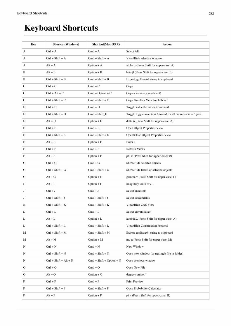
Keyboard Shortcuts 281

Keyboard Shortcuts

Key Shortcut(Windows) Shortcut(Mac OS X) Action

A Ctrl + A Cmd + A Select All

A Ctrl + Shift + A Cmd + Shift + A View/Hide Algebra Window

A Alt + A Option + A alpha α (Press Shift for upper-case: Α)

B Alt + B Option + B beta β (Press Shift for upper-case: Β)

B Ctrl + Shift + B Cmd + Shift + B Export ggbBase64 string to clipboard

C Ctrl + C Cmd + C Copy

C Ctrl + Alt + C Cmd + Option + C Copies values (spreadsheet)

C Ctrl + Shift + C Cmd + Shift + C Copy Graphics View to clipboard

D Ctrl + D Cmd + D Toggle value/definition/command

D Ctrl + Shift + D Cmd + Shift_D Toggle toggle Selection Allowed for all "non-essential" geos

D Alt + D Option + D delta δ (Press Shift for upper-case: Δ)

E Ctrl + E Cmd + E Open Object Properties View

E Ctrl + Shift + E Cmd + Shift + E Open/Close Object Properties View

E Alt + E Option + E Euler ℯ

F Ctrl + F Cmd + F Refresh Views

F Alt + F Option + F phi φ (Press Shift for upper-case: Φ)

G Ctrl + G Cmd + G Show/Hide selected objects

G Ctrl + Shift + G Cmd + Shift + G Show/Hide labels of selected objects

G Alt + G Option + G gamma γ (Press Shift for upper-case: Γ)

I Alt + I Option + I imaginary unit ί = √-1

J Ctrl + J Cmd + J Select ancestors

J Ctrl + Shift + J Cmd + Shift + J Select descendants

K Ctrl + Shift + K Cmd + Shift + K View/Hide CAS View

L Ctrl + L Cmd + L Select current layer

L Alt + L Option + L lambda λ (Press Shift for upper-case: Λ)

L Ctrl + Shift + L Cmd + Shift + L View/Hide Construction Protocol

M Ctrl + Shift + M Cmd + Shift + M Export ggbBase64 string to clipboard

M Alt + M Option + M mu μ (Press Shift for upper-case: Μ)

N Ctrl + N Cmd + N New Window

N Ctrl + Shift + N Cmd + Shift + N Open next window (or next ggb file in folder)

N Ctrl + Shift + Alt + N Cmd + Shift + Option + N Open previous window

O Ctrl + O Cmd + O Open New File

O Alt + O Option + O degree symbol °

P Ctrl + P Cmd + P Print Preview

P Ctrl + Shift + P Cmd + Shift + P Open Probability Calculator

P Alt + P Option + P pi π (Press Shift for upper-case: Π)

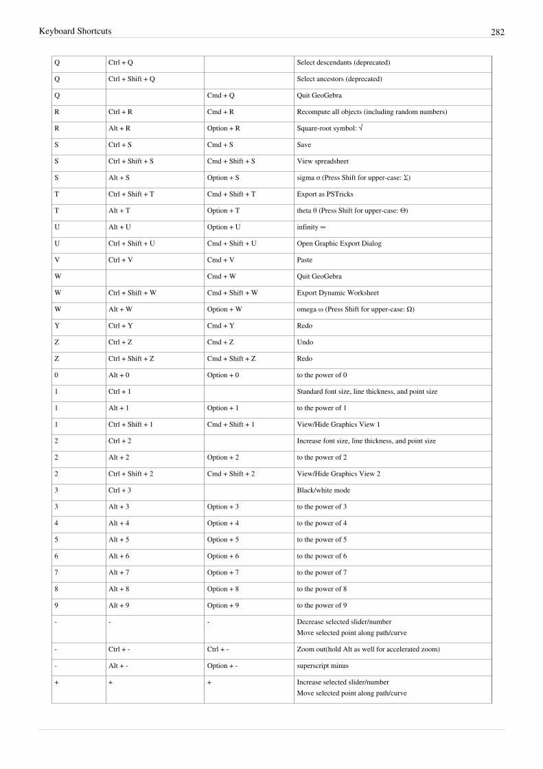
Keyboard Shortcuts 282

Q Ctrl + Q Select descendants (deprecated)

Q Ctrl + Shift + Q Select ancestors (deprecated)

Q Cmd + Q Quit GeoGebra

R Ctrl + R Cmd + R Recompute all objects (including random numbers)

R Alt + R Option + R Square-root symbol: √

S Ctrl + S Cmd + S Save

S Ctrl + Shift + S Cmd + Shift + S View spreadsheet

S Alt + S Option + S sigma σ (Press Shift for upper-case: Σ)

T Ctrl + Shift + T Cmd + Shift + T Export as PSTricks

T Alt + T Option + T theta θ (Press Shift for upper-case: Θ)

U Alt + U Option + U infinity ∞

U Ctrl + Shift + U Cmd + Shift + U Open Graphic Export Dialog

V Ctrl + V Cmd + V Paste

W Cmd + W Quit GeoGebra

W Ctrl + Shift + W Cmd + Shift + W Export Dynamic Worksheet

W Alt + W Option + W omega ω (Press Shift for upper-case: Ω)

Y Ctrl + Y Cmd + Y Redo

Z Ctrl + Z Cmd + Z Undo

Z Ctrl + Shift + Z Cmd + Shift + Z Redo

0 Alt + 0 Option + 0 to the power of 0

1 Ctrl + 1 Standard font size, line thickness, and point size

1 Alt + 1 Option + 1 to the power of 1

1 Ctrl + Shift + 1 Cmd + Shift + 1 View/Hide Graphics View 1

2 Ctrl + 2 Increase font size, line thickness, and point size

2 Alt + 2 Option + 2 to the power of 2

2 Ctrl + Shift + 2 Cmd + Shift + 2 View/Hide Graphics View 2

3 Ctrl + 3 Black/white mode

3 Alt + 3 Option + 3 to the power of 3

4 Alt + 4 Option + 4 to the power of 4

5 Alt + 5 Option + 5 to the power of 5

6 Alt + 6 Option + 6 to the power of 6

7 Alt + 7 Option + 7 to the power of 7

8 Alt + 8 Option + 8 to the power of 8

9 Alt + 9 Option + 9 to the power of 9

- - - Decrease selected slider/numberMove selected point along path/curve

- Ctrl + - Ctrl + - Zoom out(hold Alt as well for accelerated zoom)

- Alt + - Option + - superscript minus

+ + + Increase selected slider/numberMove selected point along path/curve

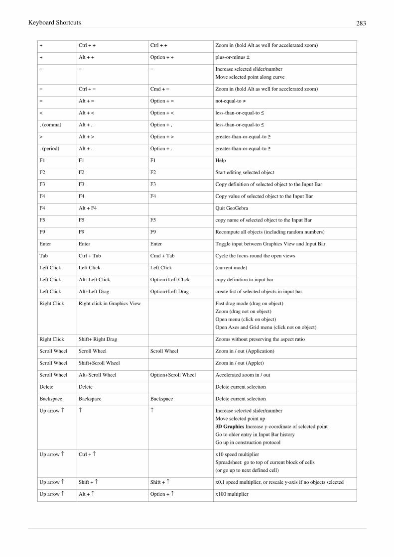
Keyboard Shortcuts 283

+ Ctrl + + Ctrl + + Zoom in (hold Alt as well for accelerated zoom)

+ Alt + + Option + + plus-or-minus ±

= = = Increase selected slider/numberMove selected point along curve

= Ctrl + = Cmd + = Zoom in (hold Alt as well for accelerated zoom)

= Alt + = Option + = not-equal-to ≠

< Alt + < Option + < less-than-or-equal-to ≤

, (comma) Alt + , Option + , less-than-or-equal-to ≤

> Alt + > Option + > greater-than-or-equal-to ≥

. (period) Alt + . Option + . greater-than-or-equal-to ≥

F1 F1 F1 Help

F2 F2 F2 Start editing selected object

F3 F3 F3 Copy definition of selected object to the Input Bar

F4 F4 F4 Copy value of selected object to the Input Bar

F4 Alt + F4 Quit GeoGebra

F5 F5 F5 copy name of selected object to the Input Bar

F9 F9 F9 Recompute all objects (including random numbers)

Enter Enter Enter Toggle input between Graphics View and Input Bar

Tab Ctrl + Tab Cmd + Tab Cycle the focus round the open views

Left Click Left Click Left Click (current mode)

Left Click Alt+Left Click Option+Left Click copy definition to input bar

Left Click Alt+Left Drag Option+Left Drag create list of selected objects in input bar

Right Click Right click in Graphics View Fast drag mode (drag on object)Zoom (drag not on object)Open menu (click on object)Open Axes and Grid menu (click not on object)

Right Click Shift+ Right Drag Zooms without preserving the aspect ratio

Scroll Wheel Scroll Wheel Scroll Wheel Zoom in / out (Application)

Scroll Wheel Shift+Scroll Wheel Zoom in / out (Applet)

Scroll Wheel Alt+Scroll Wheel Option+Scroll Wheel Accelerated zoom in / out

Delete Delete Delete current selection

Backspace Backspace Backspace Delete current selection

Up arrow ↑ ↑ ↑ Increase selected slider/numberMove selected point up3D Graphics Increase y-coordinate of selected pointGo to older entry in Input Bar historyGo up in construction protocol

Up arrow ↑ Ctrl + ↑ x10 speed multiplierSpreadsheet: go to top of current block of cells(or go up to next defined cell)

Up arrow ↑ Shift + ↑ Shift + ↑ x0.1 speed multiplier, or rescale y-axis if no objects selected

Up arrow ↑ Alt + ↑ Option + ↑ x100 multiplier

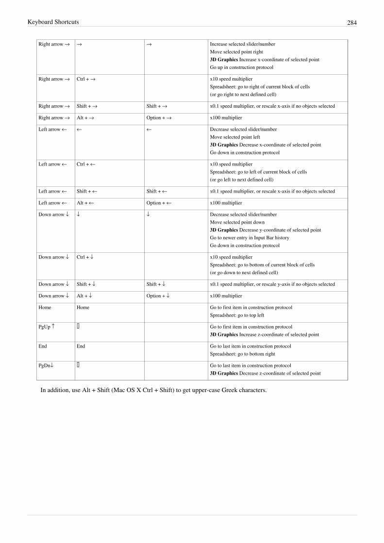
Keyboard Shortcuts 284

Right arrow → → → Increase selected slider/numberMove selected point right3D Graphics Increase x-coordinate of selected pointGo up in construction protocol

Right arrow → Ctrl + → x10 speed multiplierSpreadsheet: go to right of current block of cells(or go right to next defined cell)

Right arrow → Shift + → Shift + → x0.1 speed multiplier, or rescale x-axis if no objects selected

Right arrow → Alt + → Option + → x100 multiplier

Left arrow ← ← ← Decrease selected slider/numberMove selected point left3D Graphics Decrease x-coordinate of selected pointGo down in construction protocol

Left arrow ← Ctrl + ← x10 speed multiplierSpreadsheet: go to left of current block of cells(or go left to next defined cell)

Left arrow ← Shift + ← Shift + ← x0.1 speed multiplier, or rescale x-axis if no objects selected

Left arrow ← Alt + ← Option + ← x100 multiplier

Down arrow ↓ ↓ ↓ Decrease selected slider/numberMove selected point down3D Graphics Decrease y-coordinate of selected pointGo to newer entry in Input Bar historyGo down in construction protocol

Down arrow ↓ Ctrl + ↓ x10 speed multiplierSpreadsheet: go to bottom of current block of cells(or go down to next defined cell)

Down arrow ↓ Shift + ↓ Shift + ↓ x0.1 speed multiplier, or rescale y-axis if no objects selected

Down arrow ↓ Alt + ↓ Option + ↓ x100 multiplier

Home Home Go to first item in construction protocolSpreadsheet: go to top left

PgUp ↑ ⇞ Go to first item in construction protocol3D Graphics Increase z-coordinate of selected point

End End Go to last item in construction protocolSpreadsheet: go to bottom right

PgDn↓ ⇟ Go to last item in construction protocol3D Graphics Decrease z-coordinate of selected point

In addition, use Alt + Shift (Mac OS X Ctrl + Shift) to get upper-case Greek characters.

Settings Dialog 285

Settings Dialog

This dialog is available by selecting the Advanced item in Options Menu, or by clicking the Preferencesicon on the toolbar. It is divided into different sections, which are shown depending on active objects and Views: Properties, Graphics, CAS, Spreadsheet, Layout, Defaults, and Advanced.

PropertiesThis section is displayed only if an object is currently selected in the construction. Clicking on the related icondisplays the Properties Dialog of the object.

GraphicsThis section is displayed only if the Graphics View is active, and allows you to define its settings, e.g. backgroundcolour, axes and grid. See Customizing the Graphics View for further details.

CASThis section is displayed only if the CAS View is active, and allows you to:• set a timeout for the CAS calculations, in seconds•• set how to show rational exponents

SpreadsheetThis section is displayed only if the Spreadsheet View is active, and contains two tabs.• The Layout tab allows you fully customize the spreadsheet, setting preferences for the input bar, grid lines,

column/row headers and scrollbars. You can also enable using buttons, checkboxes and tooltips.• The Browser tab allows you to show the files browser, and set the file system directories, as well as a remote

URL for your files.

LayoutThis section allows you to customize the layout of the main components of your GeoGebra window, setting theposition of the input bar, the toolbar, and the sidebar, as well as the style bar and title bar visibility.

DefaultsThis section allows you to customize the appearance and style of all the mathematical objects in GeoGebra. The listof all available objects is shown on the left of the dialog window, while on the right the Properties Dialog tabs areshown, where you can set visibility, colour, style and algebraic settings for all your mathematical objects.

Settings Dialog 286

AdvancedThis section contains the following advanced global settings:• Angle Unit: switch between Degree and Radians• Right Angle Style: choose the symbol for a right angle.• Coordinates: define how coordinates are displayed algebraically.• Continuity: if Continuity is On, GeoGebra tries to set new calculated points near the original ones.• Use Path and region Parameters: you can turn On and Off this option• Virtual Keyboard: options to set the virtual keyboard language, its width,height and opacity.• Checkbox Size: switch between regular and large checkboxes.• Fonts Size: set the Menu font size• Tooltips: set the tooltip language and a timeout for tooltips.• Language: use digits and point names specified for your language.• Perspectives: manage the perspectives of GeoGebra.• Miscellaneous: enable scripting, enable the use of Java fonts, set inverse trig functions values as angles and

reverse the mouse wheel zooming features.

Virtual KeyboardThe Virtual Keyboard is a semi-transparent keyboard that is displayed on the screen when the correspondingmenu item is selected.It contains the standard keyboard characters, as well as the most used mathematical symbols and operators,and can be used with a mouse or other pointing devices.This makes the Virtual Keyboard particularly useful when using GeoGebra for presentations or withmultimedia interactive whiteboards.

Tool Manager Dialog 287

Tool Manager DialogYou can save your custom tools so you can reuse them in other GeoGebra constructions. In the Tools Menu, select

Manage Tools to open this dialog. Then, select the custom tool you want to save from the appearing list. Click onbutton Save As… in order to save your custom tool on your computer.Note: User defined tools are saved as files with the file name extension GGT so you can distinguish custom tool filesfrom usual GeoGebra files (GGB).This dialog also allows you to remove or modify tools. If you decide to modify a tool, new GeoGebra windowappears. The input objects are listed as free objects in it. If you have done finishing your changes, you can save thetool via option Create new tool in Tools Menu. Keep the old name to overwrite the tool. To overwrite a toolwhich was already used, the types of input and output objects must stay the same.

Accessibility

Mouse controlGeoGebra has an embedded virtual keyboard that allows the user to interact with the software using the mouse.Select View → Keyboard to open the virtual keyboard and start using it with the mouse.Note: Besides the standard layout, the virtual keyboard also contains a selection of mathematical symbols. Furthercharacters are available by pressing the AltG button.The virtual keyboard can also be resized, by dragging its edges.

Keyboard controlTo open menus using keyboard only, press Alt and arrows (on Windows). On Mac you have to enable full keyboardaccess first. Press Ctrl + F1 to activate it. Now you are able to select menus by using Ctrl + F2 or on some keyboardsFn + Ctrl + F2. For more keyboard options see the Keyboard Shortcuts section. Moreover, all features of theProperties Dialog are accessible via Scripting Commands.

288

Publishing

Creating Pictures of the Graphics ViewYou can either save a picture of the Graphics View in a file or copy it to clipboard.

Saving as FileNote: The full Graphics View will be saved as a picture, unless points Export_1 and Export_2 are defined (seebelow).If your construction does not use all the available space in the Graphics View, you might want to…

• …use tools Move Graphics View Tool, Zoom In Tool and/or Zoom Out Tool in order to placeyour construction in the upper left corner of the Graphics View. Afterwards, you may reduce the size of theGeoGebra window by dragging one of its corners with the mouse.

• … use the selection rectangle in order to specify which part of the Graphics View should be exported and savedas a picture.

You create points called Export_1 and Export_2, which will be used to define diagonally opposite corners of theexport rectangle.Note: Points Export1 and Export2 must be within the visible area of the Graphics View.In the File Menu, select item Export before clicking on item Graphics View as Picture. In the appearing dialogwindow you may specify the Format, Scale (in cm), and the Resolution (in dpi) of the output picture file.Note: The true size of the exported image is shown at the bottom of the export window just above the buttons, bothin centimeters and pixel.Please find more information about the different picture files available in section Export Graphics Dialog.

Copying the Graphics View to ClipboardYou can also copy the Graphics View to the Clipboard of your computer: just select File – Export – GraphicsView as Picture (png, eps)…, then click the Clipboard button.This feature copies a screenshot of the Graphics View to your system's clipboard as a PNG picture. This picture canbe pasted into other documents (e. g. a word processing document).Notes:The File – Export – Graphics View as Picture (png, eps)… option allows you to define the dimension (scaleor pixels) of the exported image.The copy to Clipboard feature is not available for Mac Os.

Upload to GeoGebraTube 289

Upload to GeoGebraTubeThere are two ways to upload a file to GeoGebraTube [1] directly from GeoGebra. First one is using the Export

Worksheet Dialog, second one is using the Share... option in File Menu.Note: This feature requires an active internet connection to work correctly.In the first step GeoGebra is going to prepare your worksheet for upload to GeoGebraTube, afterwards your browsershould open up and load a website which leads you through the process of publishing your worksheet onGeoGebraTube. More information about GeoGebraTube and its usage can be found in the wiki section [1].Note: You can cancel the uploading process at any time by closing the browser window.

Export as html WebpageTo create a webpage including interactive GeoGebra construction, you have to upload the construction toGeoGebraTube and use the Embed button in the teacher page.You can then paste the resulting code into your online content management system or you can save it as .html fileusing a text editor like Notepad and add texts above and below the construction.

Advanced settingsThe Advanced Settings button allows you to change the functionality of the dynamic construction (e. g., show a reseticon and browser features) as well as to modify the user interface shown in the interactive applet (e. g., show theToolbar, modify height and width, enabling saving and printing, and others).Note: If the size of your applet is too big to fit on a computer screen with standard resolution (1024 x 768), you maywant to resize it before the actual export as a Dynamic Worksheet.Functionality:• Enable right click, zooming and keyboard editing features: By selecting this feature you will be able to right click

objects or the drawing pad in order to access the features of the context menu (e.g. show / hide object or label,trace on / off, Properties dialog). It is also possible to use the common keyboard shortcuts.

• Enable dragging of labels: By selecting this feature you are able to drag labels of points or objects.• Show icon to reset construction: A reset icon is displayed in the upper right corner of the interactive applet

allowing your students to reset the interactive figure to its initial state.User interface:• Show menubar: The menubar is displayed within the interactive applet.• Show toolbar: The toolbar is displayed within the interactive applet allowing to use the geometry tools.• Show inputbar: The input field is displayed at the bottom of the interactive applet allowing to use algebraic input

and commands for explorations.Note: If you reduce the size of the applet important parts of the dynamic worksheets might be invisible for users.

Hint: If you include the menubar, toolbar, or input field you might want to adjust the height of the interactiveapplet.

Embedding to CMS, VLE (Moodle) and Wiki 290

Embedding to CMS, VLE (Moodle) and WikiTo create a webpage including interactive GeoGebra construction, you have to upload the construction toGeoGebraTube and use the Embed button in the teacher page.You can then paste the resulting code into your online content management system or you can save it as .html fileusing a text editor like Notepad and add texts above and below the construction.

Advanced settingsThe Advanced Settings button allows you to change the functionality of the dynamic construction (e. g., show a reseticon and browser features) as well as to modify the user interface shown in the interactive applet (e. g., show theToolbar, modify height and width, enabling saving and printing, and others).Note: If the size of your applet is too big to fit on a computer screen with standard resolution (1024 x 768), you maywant to resize it before the actual export as a Dynamic Worksheet.Functionality:• Enable right click, zooming and keyboard editing features: By selecting this feature you will be able to right click

objects or the drawing pad in order to access the features of the context menu (e.g. show / hide object or label,trace on / off, Properties dialog). It is also possible to use the common keyboard shortcuts.

• Enable dragging of labels: By selecting this feature you are able to drag labels of points or objects.• Show icon to reset construction: A reset icon is displayed in the upper right corner of the interactive applet

allowing your students to reset the interactive figure to its initial state.User interface:• Show menubar: The menubar is displayed within the interactive applet.• Show toolbar: The toolbar is displayed within the interactive applet allowing to use the geometry tools.• Show inputbar: The input field is displayed at the bottom of the interactive applet allowing to use algebraic input

and commands for explorations.Note: If you reduce the size of the applet important parts of the dynamic worksheets might be invisible for users.

Hint: If you include the menubar, toolbar, or input field you might want to adjust the height of the interactiveapplet.

Export to LaTeX (PGF, PSTricks) and Asymptote 291

Export to LaTeX (PGF, PSTricks) andAsymptote

Export - Graphics View as Animated GIF...When the dynamic construction depends on a slider, this menu item allows you to save the Graphics View as anAnimated GIF. Just drag a selection rectangle around the portion of the construction you need to export (or resize theGeoGebra window), then select File -> Export -> Graphics View as Animated GIF. A dialog will let you choose theanimating slider name, as well as the timing between frames and the option to display the animation as loop.

Export - Graphics View as PSTricks…Keyboard shortcut: Ctrl + Shift + T (MacOS: Cmd + Shift + T)

This menu item allows you to save the Graphics View as a PSTricks [1] picture file, which is a LaTeX picture format.

Export - Graphics View as PGF/TiKZ…This menu item allows you to save the Graphics View as a PGF [2] picture file, which is a LaTeX picture format.

Export - Graphics View as Asymptote…This menu item allows you to save the Graphics View as a Asymptote [3] picture file.

Limits of these export functionsApart from Animated GIF export, these exports work only for the 2D View and the following object types can't beexported•• implicit curves•• loci

Printing Options 292

Printing Options

Printing the Graphics ViewGeoGebra allows you to print the Graphics View of your constructions. You can find the corresponding item PrintPreview in the File Menu. In the appearing Print Preview Dialog window, you can specify the Title, Author, and aDate for the construction. In addition, you can set the Scale of your printout (in cm) and change the Orientation ofthe paper used (portrait or landscape).Note: In order to update the Print Preview after you made changes to the text or layout of the printout, you need topress Enter.

Printing the Construction ProtocolIf you want to print the Construction Protocol, you first need to open the Construction Protocol dialog window byusing the View menu. Then, select Print... from the File menu of this new window.The Print dialog window allows you to enter the Author or change the paper Margins and Orientation before printingthe Construction Protocol.Note: You may switch the different columns Name, Definition, Command, Algebra, and Breakpoint of theConstruction Protocol on and off by using the View menu of the Construction Protocol dialog window.

Article Sources and Contributors 293

Article Sources and ContributorsIntroduction  Source: http://wiki.geogebra.org/s/en/index.php?oldid=43173  Contributors: Administrator, Christina.biermair, Florian Sonner, Jhohen, Markus, MediaWiki default, Murkle, NoelLambert, Spam cleanup script, Spanish1, Zbynek

Compatibility  Source: http://wiki.geogebra.org/s/en/index.php?oldid=43233  Contributors: Markus, Murkle, Zbynek

Installation Guide  Source: http://wiki.geogebra.org/s/en/index.php?oldid=44049  Contributors: Kovács Zoltán, Mathmum, Murkle, Spanish1, Wkuellinger, davidfruelund

Free, Dependent and Auxiliary Objects  Source: http://wiki.geogebra.org/s/en/index.php?oldid=42065  Contributors: Andrea.duringer, Jhohen, Mathmum, Zbynek

Geometric Objects  Source: http://wiki.geogebra.org/s/en/index.php?oldid=43713  Contributors: Jhohen, Mathmum, Zbynek

Points and Vectors  Source: http://wiki.geogebra.org/s/en/index.php?oldid=38481  Contributors: Andrea.duringer, Mathmum, Murkle, Zbynek

Lines and Axes  Source: http://wiki.geogebra.org/s/en/index.php?oldid=34184  Contributors: Andrea.duringer, Mathmum, Murkle, Zbynek

Conic sections  Source: http://wiki.geogebra.org/s/en/index.php?oldid=34122  Contributors: Mathmum, Zbynek

Functions  Source: http://wiki.geogebra.org/s/en/index.php?oldid=39053  Contributors: Mathmum, Zbynek

Curves  Source: http://wiki.geogebra.org/s/en/index.php?oldid=39425  Contributors: Andrea.duringer, Mathmum, Murkle, Zbynek

Inequalities  Source: http://wiki.geogebra.org/s/en/index.php?oldid=34430  Contributors: Birgit Lachner, Mathmum, Zbynek

Intervals  Source: http://wiki.geogebra.org/s/en/index.php?oldid=34165  Contributors: Mathmum, Zbynek

General Objects  Source: http://wiki.geogebra.org/s/en/index.php?oldid=34419  Contributors: Mathmum, Zbynek

Numbers and Angles  Source: http://wiki.geogebra.org/s/en/index.php?oldid=34499  Contributors: Mathmum, Zbynek

Texts  Source: http://wiki.geogebra.org/s/en/index.php?oldid=34599  Contributors: Andrea.duringer, Mathmum, Murkle, Zbynek

Boolean values  Source: http://wiki.geogebra.org/s/en/index.php?oldid=38389  Contributors: Mathmum, Zbynek

Complex Numbers  Source: http://wiki.geogebra.org/s/en/index.php?oldid=42043  Contributors: Andrea.duringer, Mathmum, Zbynek

Lists  Source: http://wiki.geogebra.org/s/en/index.php?oldid=34469  Contributors: Andrea.duringer, Mathmum, Murkle, Noel Lambert, Zbynek

Matrices  Source: http://wiki.geogebra.org/s/en/index.php?oldid=41244  Contributors: Mathmum, Zbynek

Action Objects  Source: http://wiki.geogebra.org/s/en/index.php?oldid=38421  Contributors: Mathmum, Zbynek

Selecting objects  Source: http://wiki.geogebra.org/s/en/index.php?oldid=38861  Contributors: Mathmum, Zbynek

Change Values  Source: http://wiki.geogebra.org/s/en/index.php?oldid=38860  Contributors: Mathmum, Zbynek

Naming Objects  Source: http://wiki.geogebra.org/s/en/index.php?oldid=42041  Contributors: Andrea.duringer, Markus, Mathmum, Murkle, Zbynek

Animation  Source: http://wiki.geogebra.org/s/en/index.php?oldid=34311  Contributors: Florian Sonner, Mathmum, Zbynek

Tracing  Source: http://wiki.geogebra.org/s/en/index.php?oldid=34604  Contributors: Mathmum, Zbynek

Object Properties  Source: http://wiki.geogebra.org/s/en/index.php?oldid=39025  Contributors: Andrea.duringer, Mathmum, Zbynek

Labels and Captions  Source: http://wiki.geogebra.org/s/en/index.php?oldid=34805  Contributors: Birgit Lachner, Mathmum, Murkle, Spanish1, Zbynek

Advanced Features  Source: http://wiki.geogebra.org/s/en/index.php?oldid=34308  Contributors: Mathmum, Zbynek

Object Position  Source: http://wiki.geogebra.org/s/en/index.php?oldid=34196  Contributors: Andrea.duringer, Zbynek

Conditional Visibility  Source: http://wiki.geogebra.org/s/en/index.php?oldid=38390  Contributors: Mathmum, Zbynek

Dynamic Colors  Source: http://wiki.geogebra.org/s/en/index.php?oldid=39811  Contributors: Mathmum, Zbynek

LaTeX  Source: http://wiki.geogebra.org/s/en/index.php?oldid=41241  Contributors: Birgit Lachner, Mathmum, Murkle, Zbynek

Layers  Source: http://wiki.geogebra.org/s/en/index.php?oldid=34461  Contributors: Andrea.duringer, Mathmum, Zbynek

Scripting  Source: http://wiki.geogebra.org/s/en/index.php?oldid=39475  Contributors: Birgit Lachner, Corinna, Mathmum, Murkle, Zbynek

Tooltips  Source: http://wiki.geogebra.org/s/en/index.php?oldid=34289  Contributors: Zbynek

Tools  Source: http://wiki.geogebra.org/s/en/index.php?oldid=43379  Contributors: Jhohen, Mathmum, Zbynek

Movement Tools  Source: http://wiki.geogebra.org/s/en/index.php?oldid=34492  Contributors: Mathmum, Zbynek

Move Tool  Source: http://wiki.geogebra.org/s/en/index.php?oldid=42039  Contributors: Florian Sonner, Jhohen, K Voss, Mathmum, Zbynek

Record to Spreadsheet Tool  Source: http://wiki.geogebra.org/s/en/index.php?oldid=41388  Contributors: K Voss, Mathmum, Sarah., Zbynek

Rotate around Point Tool  Source: http://wiki.geogebra.org/s/en/index.php?oldid=43801  Contributors: Mathmum, Zbynek

Point Tools  Source: http://wiki.geogebra.org/s/en/index.php?oldid=41887  Contributors: Jhohen, Mathmum, Zbynek

Point Tool  Source: http://wiki.geogebra.org/s/en/index.php?oldid=38519  Contributors: K Voss, Mathmum, Zbynek

Attach / Detach Point Tool  Source: http://wiki.geogebra.org/s/en/index.php?oldid=34312  Contributors: Zbynek

Complex Number Tool  Source: http://wiki.geogebra.org/s/en/index.php?oldid=34342  Contributors: Murkle, Zbynek

Point on Object Tool  Source: http://wiki.geogebra.org/s/en/index.php?oldid=34516  Contributors: Andrea.duringer, Murkle, Zbynek

Intersect Tool  Source: http://wiki.geogebra.org/s/en/index.php?oldid=38313  Contributors: K Voss, Mathmum, Zbynek

Midpoint or Center Tool  Source: http://wiki.geogebra.org/s/en/index.php?oldid=38634  Contributors: K Voss, Mathmum, Zbynek

Line Tools  Source: http://wiki.geogebra.org/s/en/index.php?oldid=38500  Contributors: Mathmum, Zbynek

Article Sources and Contributors 294

Line Tool  Source: http://wiki.geogebra.org/s/en/index.php?oldid=38336  Contributors: K Voss, Mathmum, Spanish1, Zbynek

Segment Tool  Source: http://wiki.geogebra.org/s/en/index.php?oldid=38344  Contributors: K Voss, Mathmum, Zbynek

Segment with Given Length Tool  Source: http://wiki.geogebra.org/s/en/index.php?oldid=38394  Contributors: K Voss, Mathmum, Zbynek

Ray Tool  Source: http://wiki.geogebra.org/s/en/index.php?oldid=38341  Contributors: K Voss, Mathmum, Zbynek

Vector from Point Tool  Source: http://wiki.geogebra.org/s/en/index.php?oldid=34624  Contributors: K Voss, Mathmum, Zbynek

Vector Tool  Source: http://wiki.geogebra.org/s/en/index.php?oldid=38339  Contributors: K Voss, Mathmum, Zbynek

Special Line Tools  Source: http://wiki.geogebra.org/s/en/index.php?oldid=34579  Contributors: Mathmum, Zbynek

Best Fit Line Tool  Source: http://wiki.geogebra.org/s/en/index.php?oldid=34101  Contributors: K Voss, Mathmum, Zbynek

Parallel Line Tool  Source: http://wiki.geogebra.org/s/en/index.php?oldid=34509  Contributors: K Voss, Mathmum, Zbynek

Angle Bisector Tool  Source: http://wiki.geogebra.org/s/en/index.php?oldid=39170  Contributors: K Voss, Mathmum, Zbynek

Perpendicular Line Tool  Source: http://wiki.geogebra.org/s/en/index.php?oldid=40504  Contributors: Johanna, K Voss, Mathmum, Zbynek

Tangents Tool  Source: http://wiki.geogebra.org/s/en/index.php?oldid=34594  Contributors: K Voss, Mathmum, Murkle, Zbynek

Polar or Diameter Line Tool  Source: http://wiki.geogebra.org/s/en/index.php?oldid=34518  Contributors: K Voss, Mathmum, Zbynek

Perpendicular Bisector Tool  Source: http://wiki.geogebra.org/s/en/index.php?oldid=39171  Contributors: K Voss, Mathmum, Zbynek

Locus Tool  Source: http://wiki.geogebra.org/s/en/index.php?oldid=38508  Contributors: Andrea.duringer, K Voss, Mathmum, Zbynek

Polygon Tools  Source: http://wiki.geogebra.org/s/en/index.php?oldid=34521  Contributors: Mathmum, Zbynek

Rigid Polygon Tool  Source: http://wiki.geogebra.org/s/en/index.php?oldid=36924  Contributors: Mathmum, Zbynek

Polyline Tool  Source: http://wiki.geogebra.org/s/en/index.php?oldid=34522  Contributors: Mathmum, Zbynek

Regular Polygon Tool  Source: http://wiki.geogebra.org/s/en/index.php?oldid=36923  Contributors: K Voss, Mathmum, Zbynek

Polygon Tool  Source: http://wiki.geogebra.org/s/en/index.php?oldid=36922  Contributors: K Voss, Mathmum, Zbynek

Circle & Arc Tools  Source: http://wiki.geogebra.org/s/en/index.php?oldid=38384  Contributors: Mathmum, Zbynek

Circle with Center and Radius Tool  Source: http://wiki.geogebra.org/s/en/index.php?oldid=36914  Contributors: K Voss, Mathmum, Zbynek

Circle through 3 Points Tool  Source: http://wiki.geogebra.org/s/en/index.php?oldid=38364  Contributors: Andrea.duringer, K Voss, Mathmum, Zbynek

Circle with Center through Point Tool  Source: http://wiki.geogebra.org/s/en/index.php?oldid=34325  Contributors: Administrator, K Voss, Mathmum, Zbynek

Circumcircular Arc Tool  Source: http://wiki.geogebra.org/s/en/index.php?oldid=38360  Contributors: K Voss, Mathmum, Zbynek

Circumcircular Sector Tool  Source: http://wiki.geogebra.org/s/en/index.php?oldid=38363  Contributors: K Voss, Mathmum, Zbynek

Compass Tool  Source: http://wiki.geogebra.org/s/en/index.php?oldid=34340  Contributors: Administrator, K Voss, Mathmum, Zbynek

Circular Sector Tool  Source: http://wiki.geogebra.org/s/en/index.php?oldid=38387  Contributors: K Voss, Mathmum, Zbynek

Semicircle through 2 Points Tool  Source: http://wiki.geogebra.org/s/en/index.php?oldid=38367  Contributors: Mathmum, Zbynek

Circular Arc Tool  Source: http://wiki.geogebra.org/s/en/index.php?oldid=38386  Contributors: K Voss, Mathmum, Zbynek

Conic Section Tools  Source: http://wiki.geogebra.org/s/en/index.php?oldid=38495  Contributors: Christina.biermair, Mathmum, Zbynek

Ellipse Tool  Source: http://wiki.geogebra.org/s/en/index.php?oldid=36904  Contributors: Administrator, Florian Sonner, K Voss, Mathmum, Zbynek

Hyperbola Tool  Source: http://wiki.geogebra.org/s/en/index.php?oldid=36903  Contributors: K Voss, Mathmum, Zbynek

Conic through 5 Points Tool  Source: http://wiki.geogebra.org/s/en/index.php?oldid=38351  Contributors: K Voss, Mathmum, Zbynek

Parabola Tool  Source: http://wiki.geogebra.org/s/en/index.php?oldid=39858  Contributors: K Voss, Mathmum, Zbynek

Measurement Tools  Source: http://wiki.geogebra.org/s/en/index.php?oldid=34480  Contributors: Christina.biermair, Mathmum, Zbynek

Distance or Length Tool  Source: http://wiki.geogebra.org/s/en/index.php?oldid=37746  Contributors: K Voss, Mathmum, Zbynek

Angle Tool  Source: http://wiki.geogebra.org/s/en/index.php?oldid=39172  Contributors: K Voss, Mathmum, Zbynek

Slope Tool  Source: http://wiki.geogebra.org/s/en/index.php?oldid=34576  Contributors: K Voss, Mathmum, Zbynek

Area Tool  Source: http://wiki.geogebra.org/s/en/index.php?oldid=39179  Contributors: K Voss, Mathmum, Zbynek

Angle with Given Size Tool  Source: http://wiki.geogebra.org/s/en/index.php?oldid=39173  Contributors: K Voss, Mathmum, Zbynek

Transformation Tools  Source: http://wiki.geogebra.org/s/en/index.php?oldid=38474  Contributors: Christina.biermair, Mathmum, Zbynek

Translate by Vector Tool  Source: http://wiki.geogebra.org/s/en/index.php?oldid=38276  Contributors: K Voss, Mathmum, Murkle, Zbynek

Reflect about Line Tool  Source: http://wiki.geogebra.org/s/en/index.php?oldid=38409  Contributors: K Voss, Mathmum, Zbynek

Reflect about Point Tool  Source: http://wiki.geogebra.org/s/en/index.php?oldid=38414  Contributors: K Voss, Mathmum, Zbynek

Rotate around Point Tool  Source: http://wiki.geogebra.org/s/en/index.php?oldid=43801  Contributors: Mathmum, Zbynek

Reflect about Circle Tool  Source: http://wiki.geogebra.org/s/en/index.php?oldid=43805  Contributors: K Voss, Mathmum, Murkle, Zbynek

Dilate from Point Tool  Source: http://wiki.geogebra.org/s/en/index.php?oldid=38370  Contributors: K Voss, Mathmum, Zbynek

Special Object Tools  Source: http://wiki.geogebra.org/s/en/index.php?oldid=43517  Contributors: Andrea.duringer, Christina.biermair, Jhohen, Mathmum, Zbynek

Image Tool  Source: http://wiki.geogebra.org/s/en/index.php?oldid=38318  Contributors: Mathmum, Murkle, Zbynek

Pen Tool  Source: http://wiki.geogebra.org/s/en/index.php?oldid=36853  Contributors: Mathmum, Noel Lambert, Zbynek

Article Sources and Contributors 295

Slider Tool  Source: http://wiki.geogebra.org/s/en/index.php?oldid=41164  Contributors: Andrea.duringer, Florian Sonner, K Voss, Mathmum, Murkle, Zbynek

Relation Tool  Source: http://wiki.geogebra.org/s/en/index.php?oldid=38333  Contributors: Mathmum, Zbynek

Function Inspector Tool  Source: http://wiki.geogebra.org/s/en/index.php?oldid=34416  Contributors: Andrea.duringer, Mathmum, Zbynek

Text Tool  Source: http://wiki.geogebra.org/s/en/index.php?oldid=38324  Contributors: Mathmum, Zbynek

Action Object Tools  Source: http://wiki.geogebra.org/s/en/index.php?oldid=38422  Contributors: Andrea.duringer, Christina.biermair, Mathmum, Zbynek

Check Box Tool  Source: http://wiki.geogebra.org/s/en/index.php?oldid=38348  Contributors: K Voss, Mathmum, Zbynek

Input Box Tool  Source: http://wiki.geogebra.org/s/en/index.php?oldid=38322  Contributors: Mathmum, Zbynek

Button Tool  Source: http://wiki.geogebra.org/s/en/index.php?oldid=38382  Contributors: Zbynek

General Tools  Source: http://wiki.geogebra.org/s/en/index.php?oldid=38419  Contributors: Christina.biermair, Mathmum, Zbynek

Custom Tools  Source: http://wiki.geogebra.org/s/en/index.php?oldid=38080  Contributors: Mathmum, Murkle, Zbynek

Show / Hide Label Tool  Source: http://wiki.geogebra.org/s/en/index.php?oldid=39022  Contributors: K Voss, Mathmum, Zbynek

Zoom Out Tool  Source: http://wiki.geogebra.org/s/en/index.php?oldid=39397  Contributors: K Voss, Mathmum, Zbynek

Zoom In Tool  Source: http://wiki.geogebra.org/s/en/index.php?oldid=39396  Contributors: K Voss, Mathmum, Zbynek

Delete Tool  Source: http://wiki.geogebra.org/s/en/index.php?oldid=41362  Contributors: Andrea.duringer, K Voss, Mathmum, Zbynek

Move Graphics View Tool  Source: http://wiki.geogebra.org/s/en/index.php?oldid=42089  Contributors: Jhohen, Mathmum, Zbynek

Show / Hide Object Tool  Source: http://wiki.geogebra.org/s/en/index.php?oldid=39021  Contributors: K Voss, Mathmum, Zbynek

Copy Visual Style Tool  Source: http://wiki.geogebra.org/s/en/index.php?oldid=34353  Contributors: Mathmum, Zbynek

Commands  Source: http://wiki.geogebra.org/s/en/index.php?oldid=37964  Contributors: Florian Sonner, Mathmum, Noel Lambert, Zbynek

Geometry Commands  Source: http://wiki.geogebra.org/s/en/index.php?oldid=34422  Contributors: Andrea.duringer, Mathmum, Zbynek

AffineRatio Command  Source: http://wiki.geogebra.org/s/en/index.php?oldid=36935  Contributors: JohannaZ, K Voss, Spanish1, Zbynek

Angle Command  Source: http://wiki.geogebra.org/s/en/index.php?oldid=44417  Contributors: Jackhu, JohannaZ, K Voss, Mathmum, Murkle, Noel Lambert, Spanish1, Zbynek

AngleBisector Command  Source: http://wiki.geogebra.org/s/en/index.php?oldid=40939  Contributors: Johanna, JohannaZ, K Voss, Mathmum, Spanish1, Zbynek

Arc Command  Source: http://wiki.geogebra.org/s/en/index.php?oldid=39302  Contributors: K Voss, MagdalenaSophieF, Mathmum, Noel Lambert, Zbynek

Area Command  Source: http://wiki.geogebra.org/s/en/index.php?oldid=40578  Contributors: Administrator, Johanna, JohannaZ, K Voss, Mathieu, Mathmum, Zbynek

Centroid Command  Source: http://wiki.geogebra.org/s/en/index.php?oldid=43809  Contributors: K Voss, MagdalenaSophieF, Mathmum, Spanish1, Zbynek

CircularArc Command  Source: http://wiki.geogebra.org/s/en/index.php?oldid=38385  Contributors: Andrea.duringer, JohannaZ, K Voss, Mathmum, Spanish1, Zbynek

CircularSector Command  Source: http://wiki.geogebra.org/s/en/index.php?oldid=38420  Contributors: Andrea.duringer, JohannaZ, K Voss, Mathmum, Spanish1, Zbynek

CircumcircularArc Command  Source: http://wiki.geogebra.org/s/en/index.php?oldid=38417  Contributors: Andrea.duringer, JohannaZ, K Voss, Mathmum, Spanish1, Zbynek

CircumcircularSector Command  Source: http://wiki.geogebra.org/s/en/index.php?oldid=38391  Contributors: Andrea.duringer, JohannaZ, K Voss, Mathmum, Zbynek

Circumference Command  Source: http://wiki.geogebra.org/s/en/index.php?oldid=34335  Contributors: Andrea.duringer, K Voss, Mathmum, Murkle, Zbynek

ClosestPoint Command  Source: http://wiki.geogebra.org/s/en/index.php?oldid=41923  Contributors: Andrea.duringer, Johanna, JohannaZ, MagdalenaSophieF, Murkle, Zbynek

CrossRatio Command  Source: http://wiki.geogebra.org/s/en/index.php?oldid=36934  Contributors: JohannaZ, K Voss, Mathmum, Spanish1, Zbynek

Direction Command  Source: http://wiki.geogebra.org/s/en/index.php?oldid=37251  Contributors: K Voss, MagdalenaSophieF, Mathmum, Zbynek

Distance Command  Source: http://wiki.geogebra.org/s/en/index.php?oldid=40577  Contributors: Andrea.duringer, Johanna, JohannaZ, K Voss, MagdalenaSophieF, Mathmum, Murkle, Sarah.,Zbynek

Intersect Command  Source: http://wiki.geogebra.org/s/en/index.php?oldid=41235  Contributors: Andrea.duringer, Johanna, JohannaZ, K Voss, MagdalenaSophieF, Mathmum, Murkle, NoelLambert, Sabsi, Sarah., SarahSt, Zbynek

IntersectPath Command  Source: http://wiki.geogebra.org/s/en/index.php?oldid=41291  Contributors: Mathmum, Sabsi, Sarah.

Length Command  Source: http://wiki.geogebra.org/s/en/index.php?oldid=40529  Contributors: Alexander Hartl, Andrea.duringer, Christina.biermair, Johanna, JohannaZ, K Voss, Mathieu,Mathmum, Murkle, UnTom, Zbynek

Line Command  Source: http://wiki.geogebra.org/s/en/index.php?oldid=38504  Contributors: K Voss, Kimeswenger, Mathmum, Murkle, Spanish1, Zbynek

PerpendicularBisector Command  Source: http://wiki.geogebra.org/s/en/index.php?oldid=41274  Contributors: Andrea.duringer, Gabriela Ferenczy, K Voss, MagdalenaSophieF, Mathmum,Sabsi, Sarah., Zbynek

Locus Command  Source: http://wiki.geogebra.org/s/en/index.php?oldid=34470  Contributors: Andrea.duringer, JohannaZ, K Voss, Mathmum, Murkle, Zbynek

Midpoint Command  Source: http://wiki.geogebra.org/s/en/index.php?oldid=40565  Contributors: Johanna, JohannaZ, K Voss, MagdalenaSophieF, Mathmum, Murkle, Spanish1, Zbynek

PerpendicularLine Command  Source: http://wiki.geogebra.org/s/en/index.php?oldid=43191  Contributors: Andrea.duringer, Johanna, K Voss, MagdalenaSophieF, Mathmum, Murkle, Sarah.,Zbynek

Perimeter Command  Source: http://wiki.geogebra.org/s/en/index.php?oldid=37382  Contributors: JohannaZ, K Voss, Mathmum, Murkle, Zbynek

Point Command  Source: http://wiki.geogebra.org/s/en/index.php?oldid=38800  Contributors: JohannaZ, K Voss, Mathmum, Murkle, Zbynek

PointIn Command  Source: http://wiki.geogebra.org/s/en/index.php?oldid=34211  Contributors: Andrea.duringer, Zbynek

Polyline Command  Source: http://wiki.geogebra.org/s/en/index.php?oldid=44503  Contributors: JohannaZ, MagdalenaSophieF, Mathmum, Noel Lambert, Zbynek

Polygon Command  Source: http://wiki.geogebra.org/s/en/index.php?oldid=40655  Contributors: Andrea.duringer, JohannaZ, K Voss, Mathmum, Sarah., Zbynek

Radius Command  Source: http://wiki.geogebra.org/s/en/index.php?oldid=37247  Contributors: K Voss, Kimeswenger, MagdalenaSophieF, Mathmum, Zbynek

Article Sources and Contributors 296

Ray Command  Source: http://wiki.geogebra.org/s/en/index.php?oldid=38517  Contributors: Andrea.duringer, K Voss, MagdalenaSophieF, Mathmum, Spanish1, Zbynek

RigidPolygon Command  Source: http://wiki.geogebra.org/s/en/index.php?oldid=40425  Contributors: Andrea.duringer, MagdalenaSophieF, Noel Lambert, Sarah., Zbynek

Sector Command  Source: http://wiki.geogebra.org/s/en/index.php?oldid=37301  Contributors: K Voss, MagdalenaSophieF, Mathmum, Spanish1, Zbynek

Segment Command  Source: http://wiki.geogebra.org/s/en/index.php?oldid=40572  Contributors: Andrea.duringer, Johanna, K Voss, MagdalenaSophieF, Mathmum, Murkle, Noel Lambert,Spanish1, Zbynek

Slope Command  Source: http://wiki.geogebra.org/s/en/index.php?oldid=37359  Contributors: Andrea.duringer, K Voss, MagdalenaSophieF, Mathmum, Zbynek

Tangent Command  Source: http://wiki.geogebra.org/s/en/index.php?oldid=40932  Contributors: Andrea.duringer, Johanna, JohannaZ, K Voss, Mathmum, Murkle, Noel Lambert, Sarah.,Zbynek

Vertex Command  Source: http://wiki.geogebra.org/s/en/index.php?oldid=44613  Contributors: Birgit Lachner, Johanna, K Voss, MagdalenaSophieF, Mathmum, Noel Lambert, Spanish1,Zbynek

Algebra Commands  Source: http://wiki.geogebra.org/s/en/index.php?oldid=37011  Contributors: Andrea.duringer, Mathmum, Zbynek

Div Command  Source: http://wiki.geogebra.org/s/en/index.php?oldid=34129  Contributors: Alexander Hartl, Christina.biermair, K Voss, Mathmum, UnTom, Zbynek

Expand Command  Source: http://wiki.geogebra.org/s/en/index.php?oldid=39772  Contributors: Alexander Hartl, Andrea.duringer, JohannaZ, K Voss, Mathmum, Murkle, Noel Lambert,Zbynek

Factor Command  Source: http://wiki.geogebra.org/s/en/index.php?oldid=39773  Contributors: Alexander Hartl, Christina.biermair, JohannaZ, K Voss, Mathmum, Murkle, Zbynek

GCD Command  Source: http://wiki.geogebra.org/s/en/index.php?oldid=34740  Contributors: Alexander Hartl, Christina.biermair, K Voss, Kimeswenger, Mathmum, Zbynek

LCM Command  Source: http://wiki.geogebra.org/s/en/index.php?oldid=34986  Contributors: Alexander Hartl, Andrea.duringer, JohannaZ, K Voss, Mathmum, Zbynek

Max Command  Source: http://wiki.geogebra.org/s/en/index.php?oldid=44611  Contributors: Alexander Hartl, Andrea.duringer, Christina.biermair, K Voss, MagdalenaSophieF, Mathmum,Murkle, Sarah., Spanish1, Zbynek

Min Command  Source: http://wiki.geogebra.org/s/en/index.php?oldid=44609  Contributors: Alexander Hartl, Christina.biermair, JohannaZ, K Voss, MagdalenaSophieF, Mathmum, Murkle,Sarah., Zbynek

Mod Command  Source: http://wiki.geogebra.org/s/en/index.php?oldid=43435  Contributors: Alexander Hartl, Andrea.duringer, Christina.biermair, JohannaZ, K Voss, Mathmum, Murkle,Zbynek

PrimeFactors Command  Source: http://wiki.geogebra.org/s/en/index.php?oldid=37007  Contributors: Alexander Hartl, Andrea.duringer, Christina.biermair, JohannaZ, Mathmum, Zbynek

Simplify Command  Source: http://wiki.geogebra.org/s/en/index.php?oldid=40956  Contributors: Alexander Hartl, Andrea.duringer, Christina.biermair, Gabriela Ferenczy, JohannaZ, K Voss,Mathmum, Murkle, Spanish1, Zbynek

Text Commands  Source: http://wiki.geogebra.org/s/en/index.php?oldid=38959  Contributors: Mathmum, Zbynek

FractionText Command  Source: http://wiki.geogebra.org/s/en/index.php?oldid=39165  Contributors: Andrea.duringer, K Voss, MagdalenaSophieF, Mathmum, Murkle, Noel Lambert, Zbynek

FormulaText Command  Source: http://wiki.geogebra.org/s/en/index.php?oldid=44183  Contributors: JohannaZ, K Voss, Mathmum, Zbynek

LetterToUnicode Command  Source: http://wiki.geogebra.org/s/en/index.php?oldid=35389  Contributors: JohannaZ, K Voss, MagdalenaSophieF, Mathmum, Zbynek

Ordinal Command  Source: http://wiki.geogebra.org/s/en/index.php?oldid=34198  Contributors: Mathmum, Murkle, Zbynek

RotateText Command  Source: http://wiki.geogebra.org/s/en/index.php?oldid=37042  Contributors: JohannaZ, Mathmum, Zbynek

TableText Command  Source: http://wiki.geogebra.org/s/en/index.php?oldid=44099  Contributors: JohannaZ, K Voss, Mathmum, Murkle, Noel Lambert, Spanish1, Zbynek

Text Command  Source: http://wiki.geogebra.org/s/en/index.php?oldid=37706  Contributors: JohannaZ, K Voss, Mathmum, Zbynek

TextToUnicode Command  Source: http://wiki.geogebra.org/s/en/index.php?oldid=37678  Contributors: JohannaZ, K Voss, Mathmum, Zbynek

UnicodeToLetter Command  Source: http://wiki.geogebra.org/s/en/index.php?oldid=37691  Contributors: JohannaZ, K Voss, Mathmum, Zbynek

UnicodeToText Command  Source: http://wiki.geogebra.org/s/en/index.php?oldid=37690  Contributors: JohannaZ, K Voss, Mathmum, Zbynek

VerticalText Command  Source: http://wiki.geogebra.org/s/en/index.php?oldid=34297  Contributors: Andrea.duringer, Gsturr, Murkle, Spanish1, Zbynek

Logic Commands  Source: http://wiki.geogebra.org/s/en/index.php?oldid=41272  Contributors: Mathmum, Zbynek

CountIf Command  Source: http://wiki.geogebra.org/s/en/index.php?oldid=44507  Contributors: JohannaZ, K Voss, Mathmum, Murkle, Zbynek

IsDefined Command  Source: http://wiki.geogebra.org/s/en/index.php?oldid=36936  Contributors: K Voss, MagdalenaSophieF, Mathmum, Zbynek

If Command  Source: http://wiki.geogebra.org/s/en/index.php?oldid=37642  Contributors: Christina.biermair, JohannaZ, K Voss, Mathmum, Murkle, Noel Lambert, Spanish1, Zbynek

IsInRegion Command  Source: http://wiki.geogebra.org/s/en/index.php?oldid=36937  Contributors: Andrea.duringer, Mathmum, Zbynek

IsInteger Command  Source: http://wiki.geogebra.org/s/en/index.php?oldid=36931  Contributors: K Voss, MagdalenaSophieF, Mathmum, Zbynek

KeepIf Command  Source: http://wiki.geogebra.org/s/en/index.php?oldid=37318  Contributors: Andrea.duringer, JohannaZ, K Voss, MagdalenaSophieF, Mathmum, Murkle, Zbynek

Relation Command  Source: http://wiki.geogebra.org/s/en/index.php?oldid=35380  Contributors: K Voss, MagdalenaSophieF, Mathmum, Zbynek

Functions & Calculus Commands  Source: http://wiki.geogebra.org/s/en/index.php?oldid=34417  Contributors: Andrea.duringer, Mathmum, Zbynek

Asymptote Command  Source: http://wiki.geogebra.org/s/en/index.php?oldid=37828  Contributors: JohannaZ, K Voss, Mathmum, Murkle, Zbynek

Coefficients Command  Source: http://wiki.geogebra.org/s/en/index.php?oldid=44165  Contributors: Alexander Hartl, Birgit Lachner, JohannaZ, Mathmum, Murkle, Noel Lambert, Spanish1,Zbynek

CompleteSquare Command  Source: http://wiki.geogebra.org/s/en/index.php?oldid=37672  Contributors: JohannaZ, Mathmum, Zbynek

ComplexRoot Command  Source: http://wiki.geogebra.org/s/en/index.php?oldid=34993  Contributors: Alexander Hartl, Andrea.duringer, Christina.biermair, JohannaZ, Mathmum, Zbynek

Curvature Command  Source: http://wiki.geogebra.org/s/en/index.php?oldid=40927  Contributors: Johanna, JohannaZ, K Voss, Mathmum, Zbynek

CurvatureVector Command  Source: http://wiki.geogebra.org/s/en/index.php?oldid=40929  Contributors: Johanna, JohannaZ, K Voss, Mathmum, Zbynek

Curve Command  Source: http://wiki.geogebra.org/s/en/index.php?oldid=41101  Contributors: Johanna, JohannaZ, K Voss, MagdalenaSophieF, Mathmum, Murkle, Noel Lambert, Zbynek

Article Sources and Contributors 297

Degree Command  Source: http://wiki.geogebra.org/s/en/index.php?oldid=37823  Contributors: Alexander Hartl, Andrea.duringer, Christina.biermair, JohannaZ, Mathmum, Spanish1, Zbynek

Denominator Command  Source: http://wiki.geogebra.org/s/en/index.php?oldid=43445  Contributors: Alexander Hartl, Christina.biermair, JohannaZ, Mathmum, Murkle, Zbynek

Derivative Command  Source: http://wiki.geogebra.org/s/en/index.php?oldid=37865  Contributors: Alexander Hartl, Andrea.duringer, Christina.biermair, JohannaZ, K Voss, MagdalenaSophieF,Mathmum, Murkle, UnTom, Zbynek

Extremum Command  Source: http://wiki.geogebra.org/s/en/index.php?oldid=36811  Contributors: JohannaZ, K Voss, Mathmum, Murkle, Spanish1, Zbynek

Factors Command  Source: http://wiki.geogebra.org/s/en/index.php?oldid=44523  Contributors: Alexander Hartl, MagdalenaSophieF, Mathmum, Zbynek

Function Command  Source: http://wiki.geogebra.org/s/en/index.php?oldid=41265  Contributors: Andrea.duringer, Florian Sonner, JohannaZ, K Voss, Mathmum, Murkle, Noel Lambert,Zbynek

ImplicitCurve Command  Source: http://wiki.geogebra.org/s/en/index.php?oldid=34878  Contributors: JohannaZ, Murkle, Zbynek

Integral Command  Source: http://wiki.geogebra.org/s/en/index.php?oldid=34891  Contributors: Alexander Hartl, Christina.biermair, K Voss, Kimeswenger, Mathmum, Murkle, Spanish1,Zbynek

IntegralBetween Command  Source: http://wiki.geogebra.org/s/en/index.php?oldid=37047  Contributors: Alexander Hartl, Christina.biermair, MagdalenaSophieF, Zbynek

Intersect Command  Source: http://wiki.geogebra.org/s/en/index.php?oldid=41235  Contributors: Andrea.duringer, Johanna, JohannaZ, K Voss, MagdalenaSophieF, Mathmum, Murkle, NoelLambert, Sabsi, Sarah., SarahSt, Zbynek

Iteration Command  Source: http://wiki.geogebra.org/s/en/index.php?oldid=37035  Contributors: JohannaZ, K Voss, Mathmum, Noel Lambert, Spanish1, Zbynek

IterationList Command  Source: http://wiki.geogebra.org/s/en/index.php?oldid=37885  Contributors: JohannaZ, K Voss, Mathmum, Zbynek

LeftSum Command  Source: http://wiki.geogebra.org/s/en/index.php?oldid=34970  Contributors: Andrea.duringer, JohannaZ, Kimeswenger, Mathmum, Spanish1, Zbynek

Limit Command  Source: http://wiki.geogebra.org/s/en/index.php?oldid=36983  Contributors: Alexander Hartl, Christina.biermair, JohannaZ, Kimeswenger, Mathmum, Murkle, Noel Lambert,Zbynek

LimitAbove Command  Source: http://wiki.geogebra.org/s/en/index.php?oldid=34973  Contributors: Alexander Hartl, Andrea.duringer, Christina.biermair, JohannaZ, Mathmum, Murkle,Zbynek

LimitBelow Command  Source: http://wiki.geogebra.org/s/en/index.php?oldid=34972  Contributors: Alexander Hartl, Andrea.duringer, Christina.biermair, JohannaZ, Mathmum, Murkle,Spanish1, Zbynek

LowerSum Command  Source: http://wiki.geogebra.org/s/en/index.php?oldid=35257  Contributors: JohannaZ, K Voss, Mathmum, Spanish1, Zbynek

Numerator Command  Source: http://wiki.geogebra.org/s/en/index.php?oldid=43443  Contributors: Alexander Hartl, Christina.biermair, JohannaZ, Mathmum, Murkle, Zbynek

OsculatingCircle Command  Source: http://wiki.geogebra.org/s/en/index.php?oldid=40930  Contributors: Johanna, JohannaZ, K Voss, Mathmum, Zbynek

PartialFractions Command  Source: http://wiki.geogebra.org/s/en/index.php?oldid=35265  Contributors: Alexander Hartl, Andrea.duringer, Christina.biermair, JohannaZ, Zbynek

PathParameter Command  Source: http://wiki.geogebra.org/s/en/index.php?oldid=37836  Contributors: JohannaZ, Mathmum, Zbynek

Polynomial Command  Source: http://wiki.geogebra.org/s/en/index.php?oldid=40460  Contributors: Johanna, JohannaZ, K Voss, Mathmum, Noel Lambert, Zbynek

RectangleSum Command  Source: http://wiki.geogebra.org/s/en/index.php?oldid=34221  Contributors: Mathmum, Spanish1, Zbynek

Root Command  Source: http://wiki.geogebra.org/s/en/index.php?oldid=37945  Contributors: Alexander Hartl, Christina.biermair, K Voss, MagdalenaSophieF, Mathmum, Murkle, Zbynek

RootList Command  Source: http://wiki.geogebra.org/s/en/index.php?oldid=37246  Contributors: MagdalenaSophieF, Mathmum, Zbynek

Roots Command  Source: http://wiki.geogebra.org/s/en/index.php?oldid=37944  Contributors: MagdalenaSophieF, Mathmum, Spanish1, Zbynek

SolveODE Command  Source: http://wiki.geogebra.org/s/en/index.php?oldid=37875  Contributors: Alexander Hartl, Christina.biermair, JohannaZ, MagdalenaSophieF, Markus, Mathmum,Murkle, Noel Lambert, Zbynek

TaylorPolynomial Command  Source: http://wiki.geogebra.org/s/en/index.php?oldid=37707  Contributors: Alexander Hartl, Christina.biermair, JohannaZ, K Voss, Mathmum, Zbynek

TrapezoidalSum Command  Source: http://wiki.geogebra.org/s/en/index.php?oldid=37902  Contributors: JohannaZ, K Voss, Mathmum, Spanish1, Zbynek

InflectionPoint Command  Source: http://wiki.geogebra.org/s/en/index.php?oldid=37339  Contributors: JohannaZ, K Voss, Mathmum, Zbynek

UpperSum Command  Source: http://wiki.geogebra.org/s/en/index.php?oldid=35256  Contributors: JohannaZ, K Voss, Mathmum, Spanish1, Zbynek

Conic Commands  Source: http://wiki.geogebra.org/s/en/index.php?oldid=34346  Contributors: Mathmum, Spanish1, Zbynek

Asymptote Command  Source: http://wiki.geogebra.org/s/en/index.php?oldid=37828  Contributors: JohannaZ, K Voss, Mathmum, Murkle, Zbynek

Axes Command  Source: http://wiki.geogebra.org/s/en/index.php?oldid=43813  Contributors: Johanna, K Voss, MagdalenaSophieF, Mathmum, Sarah., Zbynek

Center Command  Source: http://wiki.geogebra.org/s/en/index.php?oldid=44607  Contributors: Johanna, K Voss, MagdalenaSophieF, Mathmum, Sarah., Zbynek

Circle Command  Source: http://wiki.geogebra.org/s/en/index.php?oldid=40605  Contributors: Administrator, Johanna, JohannaZ, K Voss, Mathmum, Murkle, Spanish1, Zbynek

Conic Command  Source: http://wiki.geogebra.org/s/en/index.php?oldid=38496  Contributors: Christina.biermair, JohannaZ, K Voss, Mathmum, Zbynek

ConjugateDiameter Command  Source: http://wiki.geogebra.org/s/en/index.php?oldid=37102  Contributors: K Voss, MagdalenaSophieF, Mathmum, Spanish1, Zbynek

Directrix Command  Source: http://wiki.geogebra.org/s/en/index.php?oldid=38969  Contributors: JohannaZ, K Voss, Mathmum, Zbynek

Eccentricity Command  Source: http://wiki.geogebra.org/s/en/index.php?oldid=36925  Contributors: Mathmum, Zbynek

Ellipse Command  Source: http://wiki.geogebra.org/s/en/index.php?oldid=36941  Contributors: Administrator, JohannaZ, K Voss, Mathmum, Noel Lambert, Zbynek

LinearEccentricity Command  Source: http://wiki.geogebra.org/s/en/index.php?oldid=36957  Contributors: K Voss, MagdalenaSophieF, Mathmum, Zbynek

MajorAxis Command  Source: http://wiki.geogebra.org/s/en/index.php?oldid=36943  Contributors: JohannaZ, K Voss, Mathmum, Zbynek

SemiMajorAxisLength Command  Source: http://wiki.geogebra.org/s/en/index.php?oldid=43793  Contributors: JohannaZ, K Voss, Mathmum, Zbynek

Focus Command  Source: http://wiki.geogebra.org/s/en/index.php?oldid=38970  Contributors: K Voss, MagdalenaSophieF, Mathmum, Zbynek

Hyperbola Command  Source: http://wiki.geogebra.org/s/en/index.php?oldid=36938  Contributors: JohannaZ, K Voss, Mathmum, Zbynek

Incircle Command  Source: http://wiki.geogebra.org/s/en/index.php?oldid=34162  Contributors: Murkle, Zbynek

Article Sources and Contributors 298

Parabola Command  Source: http://wiki.geogebra.org/s/en/index.php?oldid=36908  Contributors: Andrea.duringer, JohannaZ, K Voss, Mathmum, Zbynek

Parameter Command  Source: http://wiki.geogebra.org/s/en/index.php?oldid=36958  Contributors: JohannaZ, K Voss, Mathmum, Zbynek

Polar Command  Source: http://wiki.geogebra.org/s/en/index.php?oldid=36959  Contributors: Andrea.duringer, JohannaZ, K Voss, Mathmum, Zbynek

MinorAxis Command  Source: http://wiki.geogebra.org/s/en/index.php?oldid=36944  Contributors: JohannaZ, K Voss, Mathmum, Zbynek

SemiMinorAxisLength Command  Source: http://wiki.geogebra.org/s/en/index.php?oldid=43791  Contributors: JohannaZ, K Voss, Mathmum, Zbynek

Semicircle Command  Source: http://wiki.geogebra.org/s/en/index.php?oldid=38493  Contributors: Andrea.duringer, JohannaZ, K Voss, Mathmum, Zbynek

List Commands  Source: http://wiki.geogebra.org/s/en/index.php?oldid=34468  Contributors: Andrea.duringer, Mathmum, Zbynek

Append Command  Source: http://wiki.geogebra.org/s/en/index.php?oldid=44365  Contributors: K Voss, Mathmum, Spanish1, Zbynek

Classes Command  Source: http://wiki.geogebra.org/s/en/index.php?oldid=41453  Contributors: JohannaZ, Mathmum, Murkle, Zbynek

Element Command  Source: http://wiki.geogebra.org/s/en/index.php?oldid=36781  Contributors: Alexander Hartl, Andrea.duringer, Christina.biermair, JohannaZ, K Voss, Mathmum, Murkle,UnTom, Zbynek

First Command  Source: http://wiki.geogebra.org/s/en/index.php?oldid=36787  Contributors: Alexander Hartl, Andrea.duringer, Christina.biermair, JohannaZ, K Voss, Mathmum, Murkle,Zbynek

Frequency Command  Source: http://wiki.geogebra.org/s/en/index.php?oldid=34745  Contributors: Gsturr, JohannaZ, Mathmum, Murkle, Zbynek

IndexOf Command  Source: http://wiki.geogebra.org/s/en/index.php?oldid=41085  Contributors: Gabriela Ferenczy, JohannaZ, Mathmum, Noel Lambert, Zbynek

Insert Command  Source: http://wiki.geogebra.org/s/en/index.php?oldid=36774  Contributors: JohannaZ, K Voss, Mathmum, Spanish1, Zbynek

Intersect Command  Source: http://wiki.geogebra.org/s/en/index.php?oldid=41235  Contributors: Andrea.duringer, Johanna, JohannaZ, K Voss, MagdalenaSophieF, Mathmum, Murkle, NoelLambert, Sabsi, Sarah., SarahSt, Zbynek

Intersection Command  Source: http://wiki.geogebra.org/s/en/index.php?oldid=37297  Contributors: K Voss, MagdalenaSophieF, Mathmum, Zbynek

IterationList Command  Source: http://wiki.geogebra.org/s/en/index.php?oldid=37885  Contributors: JohannaZ, K Voss, Mathmum, Zbynek

Join Command  Source: http://wiki.geogebra.org/s/en/index.php?oldid=37633  Contributors: JohannaZ, K Voss, Mathmum, Spanish1, Zbynek

Last Command  Source: http://wiki.geogebra.org/s/en/index.php?oldid=34960  Contributors: Alexander Hartl, Andrea.duringer, Christina.biermair, JohannaZ, K Voss, Mathmum, Zbynek

OrdinalRank Command  Source: http://wiki.geogebra.org/s/en/index.php?oldid=35258  Contributors: JohannaZ, Mathmum, Murkle, Zbynek

PointList Command  Source: http://wiki.geogebra.org/s/en/index.php?oldid=35316  Contributors: JohannaZ, Zbynek

Product Command  Source: http://wiki.geogebra.org/s/en/index.php?oldid=35311  Contributors: Alexander Hartl, Andrea.duringer, JohannaZ, K Voss, Mathmum, Murkle, Spanish1, UnTom,Zbynek

RandomElement Command  Source: http://wiki.geogebra.org/s/en/index.php?oldid=34219  Contributors: Christina.biermair, Murkle, UnTom, Zbynek

RemoveUndefined Command  Source: http://wiki.geogebra.org/s/en/index.php?oldid=39888  Contributors: JohannaZ, K Voss, Mathmum, Murkle, Spanish1, Zbynek

Reverse Command  Source: http://wiki.geogebra.org/s/en/index.php?oldid=37388  Contributors: JohannaZ, K Voss, MagdalenaSophieF, Mathmum, Spanish1, Zbynek

RootList Command  Source: http://wiki.geogebra.org/s/en/index.php?oldid=37246  Contributors: MagdalenaSophieF, Mathmum, Zbynek

SelectedElement Command  Source: http://wiki.geogebra.org/s/en/index.php?oldid=36897  Contributors: MagdalenaSophieF, Mathmum, Zbynek

SelectedIndex Command  Source: http://wiki.geogebra.org/s/en/index.php?oldid=36898  Contributors: MagdalenaSophieF, Mathmum, Zbynek

Sequence Command  Source: http://wiki.geogebra.org/s/en/index.php?oldid=36813  Contributors: Alexander Hartl, JohannaZ, K Voss, Mathmum, UnTom, Zbynek

Sort Command  Source: http://wiki.geogebra.org/s/en/index.php?oldid=37343  Contributors: Andrea.duringer, K Voss, MagdalenaSophieF, Mathmum, Murkle, Zbynek

Take Command  Source: http://wiki.geogebra.org/s/en/index.php?oldid=37700  Contributors: Alexander Hartl, Andrea.duringer, Christina.biermair, JohannaZ, K Voss, MagdalenaSophieF,Mathmum, Murkle, Zbynek

TiedRank Command  Source: http://wiki.geogebra.org/s/en/index.php?oldid=43817  Contributors: Andrea.duringer, JohannaZ, Mathmum, Murkle, Spanish1, Zbynek

Union Command  Source: http://wiki.geogebra.org/s/en/index.php?oldid=37644  Contributors: JohannaZ, K Voss, Mathmum, Murkle, Spanish1, Zbynek

Unique Command  Source: http://wiki.geogebra.org/s/en/index.php?oldid=44447  Contributors: Alexander Hartl, Andrea.duringer, Gsturr, JohannaZ, Mathmum, UnTom, Zbynek

Zip Command  Source: http://wiki.geogebra.org/s/en/index.php?oldid=31876  Contributors: Andrea.duringer, Mathmum, Spanish1, Zbynek

Vector & Matrix Commands  Source: http://wiki.geogebra.org/s/en/index.php?oldid=34622  Contributors: Mathmum, Zbynek

ApplyMatrix Command  Source: http://wiki.geogebra.org/s/en/index.php?oldid=43719  Contributors: MagdalenaSophieF, Mathmum, Noel Lambert, Zbynek

CurvatureVector Command  Source: http://wiki.geogebra.org/s/en/index.php?oldid=40929  Contributors: Johanna, JohannaZ, K Voss, Mathmum, Zbynek

Determinant Command  Source: http://wiki.geogebra.org/s/en/index.php?oldid=34376  Contributors: Alexander Hartl, Christina.biermair, K Voss, Mathmum, Zbynek

Identity Command  Source: http://wiki.geogebra.org/s/en/index.php?oldid=44483  Contributors: Alexander Hartl, Andrea.duringer, Christina.biermair, JohannaZ, Mathmum, Murkle, Zbynek

Invert Command  Source: http://wiki.geogebra.org/s/en/index.php?oldid=44625  Contributors: Alexander Hartl, Andrea.duringer, Christina.biermair, JohannaZ, K Voss, Mathmum, Murkle,Spanish1, UnTom, Zbynek

PerpendicularVector Command  Source: http://wiki.geogebra.org/s/en/index.php?oldid=40652  Contributors: Alexander Hartl, Andrea.duringer, Christina.biermair, K Voss,MagdalenaSophieF, Mathmum, Sarah., Zbynek

ReducedRowEchelonForm Command  Source: http://wiki.geogebra.org/s/en/index.php?oldid=37675  Contributors: Alexander Hartl, Andrea.duringer, Christina.biermair, JohannaZ, NoelLambert, Zbynek

Transpose Command  Source: http://wiki.geogebra.org/s/en/index.php?oldid=34608  Contributors: Alexander Hartl, Christina.biermair, K Voss, Mathmum, Zbynek

UnitPerpendicularVector Command  Source: http://wiki.geogebra.org/s/en/index.php?oldid=40447  Contributors: Alexander Hartl, Andrea.duringer, JohannaZ, K Voss, Mathmum, Murkle,Sarah., Zbynek

Article Sources and Contributors 299

UnitVector Command  Source: http://wiki.geogebra.org/s/en/index.php?oldid=36779  Contributors: Alexander Hartl, Andrea.duringer, Christina.biermair, JohannaZ, K Voss, Mathmum,Murkle, UnTom, Zbynek

Vector Command  Source: http://wiki.geogebra.org/s/en/index.php?oldid=38480  Contributors: Andrea.duringer, JohannaZ, K Voss, Mathmum, Murkle, Zbynek

Transformation Commands  Source: http://wiki.geogebra.org/s/en/index.php?oldid=34605  Contributors: Andrea.duringer, Mathmum, Zbynek

Dilate Command  Source: http://wiki.geogebra.org/s/en/index.php?oldid=38490  Contributors: Andrea.duringer, K Voss, MagdalenaSophieF, Mathmum, Zbynek

Reflect Command  Source: http://wiki.geogebra.org/s/en/index.php?oldid=40442  Contributors: K Voss, MagdalenaSophieF, Mathmum, Sarah., Zbynek

Rotate Command  Source: http://wiki.geogebra.org/s/en/index.php?oldid=40586  Contributors: Andrea.duringer, Johanna, JohannaZ, K Voss, Mathmum, Murkle, Noel Lambert, Zbynek

Shear Command  Source: http://wiki.geogebra.org/s/en/index.php?oldid=37786  Contributors: JohannaZ, MagdalenaSophieF, Mathmum, Zbynek

Stretch Command  Source: http://wiki.geogebra.org/s/en/index.php?oldid=37372  Contributors: MagdalenaSophieF, Murkle, Zbynek

Translate Command  Source: http://wiki.geogebra.org/s/en/index.php?oldid=38475  Contributors: Andrea.duringer, JohannaZ, K Voss, Mathmum, Zbynek

Chart Commands  Source: http://wiki.geogebra.org/s/en/index.php?oldid=34319  Contributors: Christina.biermair, Mathmum, Zbynek

BarChart Command  Source: http://wiki.geogebra.org/s/en/index.php?oldid=40865  Contributors: Gsturr, JohannaZ, K Voss, Kimeswenger, Mathmum, Sarah., Zbynek

BoxPlot Command  Source: http://wiki.geogebra.org/s/en/index.php?oldid=34726  Contributors: K Voss, Kimeswenger, Mathmum, Murkle, Zbynek

DotPlot Command  Source: http://wiki.geogebra.org/s/en/index.php?oldid=40920  Contributors: Johanna, JohannaZ, Mathmum, Sabsi, Sarah., Zbynek

FrequencyPolygon Command  Source: http://wiki.geogebra.org/s/en/index.php?oldid=36859  Contributors: JohannaZ, Mathmum, Zbynek

Histogram Command  Source: http://wiki.geogebra.org/s/en/index.php?oldid=41455  Contributors: Gsturr, JohannaZ, K Voss, Mathmum, Murkle, Zbynek

HistogramRight Command  Source: http://wiki.geogebra.org/s/en/index.php?oldid=41457  Contributors: Christina.biermair, Kimeswenger, Mathmum, Murkle, Zbynek

NormalQuantilePlot Command  Source: http://wiki.geogebra.org/s/en/index.php?oldid=37229  Contributors: Gsturr, MagdalenaSophieF, Zbynek

ResidualPlot Command  Source: http://wiki.geogebra.org/s/en/index.php?oldid=44499  Contributors: MagdalenaSophieF, Mathmum, Zbynek

StemPlot Command  Source: http://wiki.geogebra.org/s/en/index.php?oldid=37349  Contributors: Gsturr, MagdalenaSophieF, Zbynek

Statistics Commands  Source: http://wiki.geogebra.org/s/en/index.php?oldid=43523  Contributors: Andrea.duringer, Jhohen, Mathmum, Zbynek

ANOVA Command  Source: http://wiki.geogebra.org/s/en/index.php?oldid=35315  Contributors: Gsturr, MagdalenaSophieF, Mathmum, Zbynek

Classes Command  Source: http://wiki.geogebra.org/s/en/index.php?oldid=41453  Contributors: JohannaZ, Mathmum, Murkle, Zbynek

Covariance Command  Source: http://wiki.geogebra.org/s/en/index.php?oldid=35382  Contributors: Alexander Hartl, Christina.biermair, JohannaZ, K Voss, Mathmum, Zbynek

Fit Command  Source: http://wiki.geogebra.org/s/en/index.php?oldid=37790  Contributors: JohannaZ, Mathmum, Noel Lambert, Zbynek

FitExp Command  Source: http://wiki.geogebra.org/s/en/index.php?oldid=37791  Contributors: Alexander Hartl, Christina.biermair, JohannaZ, K Voss, Mathmum, Murkle, Noel Lambert,Zbynek

FitGrowth Command  Source: http://wiki.geogebra.org/s/en/index.php?oldid=37792  Contributors: JohannaZ, Mathmum, Zbynek

FitLineX Command  Source: http://wiki.geogebra.org/s/en/index.php?oldid=37806  Contributors: Andrea.duringer, JohannaZ, Zbynek

FitLine Command  Source: http://wiki.geogebra.org/s/en/index.php?oldid=37793  Contributors: Andrea.duringer, JohannaZ, K Voss, Mathmum, Zbynek

FitLog Command  Source: http://wiki.geogebra.org/s/en/index.php?oldid=37808  Contributors: Alexander Hartl, Christina.biermair, JohannaZ, K Voss, Mathmum, Zbynek

FitLogistic Command  Source: http://wiki.geogebra.org/s/en/index.php?oldid=37814  Contributors: JohannaZ, K Voss, Mathmum, Murkle, Spanish1, Zbynek

FitPoly Command  Source: http://wiki.geogebra.org/s/en/index.php?oldid=37813  Contributors: Alexander Hartl, Christina.biermair, K Voss, MagdalenaSophieF, Mathmum, Murkle, Zbynek

FitPow Command  Source: http://wiki.geogebra.org/s/en/index.php?oldid=37810  Contributors: Alexander Hartl, Andrea.duringer, Christina.biermair, K Voss, MagdalenaSophieF, Mathmum,Zbynek

FitSin Command  Source: http://wiki.geogebra.org/s/en/index.php?oldid=37811  Contributors: Alexander Hartl, Christina.biermair, K Voss, MagdalenaSophieF, Mathmum, Murkle, Zbynek

Frequency Command  Source: http://wiki.geogebra.org/s/en/index.php?oldid=34745  Contributors: Gsturr, JohannaZ, Mathmum, Murkle, Zbynek

FrequencyTable Command  Source: http://wiki.geogebra.org/s/en/index.php?oldid=40864  Contributors: Andrea.duringer, JohannaZ, Murkle, Sabsi, Zbynek

GeometricMean Command  Source: http://wiki.geogebra.org/s/en/index.php?oldid=44445  Contributors: Mathmum, Zbynek

HarmonicMean Command  Source: http://wiki.geogebra.org/s/en/index.php?oldid=44443  Contributors: JohannaZ, Mathmum, Zbynek

Mean Command  Source: http://wiki.geogebra.org/s/en/index.php?oldid=37129  Contributors: Alexander Hartl, Andrea.duringer, Christina.biermair, Gsturr, JohannaZ, K Voss,MagdalenaSophieF, Mathmum, Murkle, Zbynek

MeanX Command  Source: http://wiki.geogebra.org/s/en/index.php?oldid=35452  Contributors: JohannaZ, Zbynek

MeanY Command  Source: http://wiki.geogebra.org/s/en/index.php?oldid=35451  Contributors: JohannaZ, Zbynek

Median Command  Source: http://wiki.geogebra.org/s/en/index.php?oldid=43389  Contributors: Alexander Hartl, Andrea.duringer, Christina.biermair, JohannaZ, K Voss, MagdalenaSophieF,Mathmum, Murkle, Spanish1, Zbynek

Mode Command  Source: http://wiki.geogebra.org/s/en/index.php?oldid=34489  Contributors: K Voss, Mathmum, Spanish1, Zbynek

CorrelationCoefficient Command  Source: http://wiki.geogebra.org/s/en/index.php?oldid=35324  Contributors: JohannaZ, K Voss, Mathmum, Zbynek

Percentile Command  Source: http://wiki.geogebra.org/s/en/index.php?oldid=35266  Contributors: Andrea.duringer, Gsturr, JohannaZ, Mathmum, Zbynek

Q1 Command  Source: http://wiki.geogebra.org/s/en/index.php?oldid=35318  Contributors: JohannaZ, K Voss, Mathmum, Murkle, Zbynek

Q3 Command  Source: http://wiki.geogebra.org/s/en/index.php?oldid=35320  Contributors: JohannaZ, K Voss, Mathmum, Murkle, Zbynek

RSquare Command  Source: http://wiki.geogebra.org/s/en/index.php?oldid=37879  Contributors: Andrea.duringer, Gsturr, JohannaZ, Zbynek

RootMeanSquare Command  Source: http://wiki.geogebra.org/s/en/index.php?oldid=36722  Contributors: JohannaZ, MagdalenaSophieF, Mathmum, Zbynek

Article Sources and Contributors 300

SD Command  Source: http://wiki.geogebra.org/s/en/index.php?oldid=37352  Contributors: Alexander Hartl, Andrea.duringer, Christina.biermair, K Voss, MagdalenaSophieF, Mathmum,Murkle, Noel Lambert, Spanish1, Zbynek

SDX Command  Source: http://wiki.geogebra.org/s/en/index.php?oldid=40898  Contributors: Gabriela Ferenczy, MagdalenaSophieF, Zbynek

SDY Command  Source: http://wiki.geogebra.org/s/en/index.php?oldid=40897  Contributors: Gabriela Ferenczy, MagdalenaSophieF, Zbynek

Sxx Command  Source: http://wiki.geogebra.org/s/en/index.php?oldid=37383  Contributors: K Voss, MagdalenaSophieF, Mathmum, Zbynek

Sxy Command  Source: http://wiki.geogebra.org/s/en/index.php?oldid=37395  Contributors: K Voss, MagdalenaSophieF, Mathmum, Murkle, Zbynek

Syy Command  Source: http://wiki.geogebra.org/s/en/index.php?oldid=37385  Contributors: K Voss, MagdalenaSophieF, Murkle, Zbynek

Sample Command  Source: http://wiki.geogebra.org/s/en/index.php?oldid=37361  Contributors: Alexander Hartl, Andrea.duringer, Christina.biermair, MagdalenaSophieF, Mathmum, Zbynek

SampleSD Command  Source: http://wiki.geogebra.org/s/en/index.php?oldid=34238  Contributors: Alexander Hartl, Andrea.duringer, Christina.biermair, MagdalenaSophieF, Mathmum,Murkle, Zbynek

SampleSDX Command  Source: http://wiki.geogebra.org/s/en/index.php?oldid=37365  Contributors: MagdalenaSophieF, Zbynek

SampleSDY Command  Source: http://wiki.geogebra.org/s/en/index.php?oldid=37367  Contributors: MagdalenaSophieF, Zbynek

SampleVariance Command  Source: http://wiki.geogebra.org/s/en/index.php?oldid=37368  Contributors: Alexander Hartl, Christina.biermair, MagdalenaSophieF, Mathmum, Murkle, UnTom,Zbynek

Shuffle Command  Source: http://wiki.geogebra.org/s/en/index.php?oldid=37123  Contributors: Alexander Hartl, Andrea.duringer, Christina.biermair, MagdalenaSophieF, Murkle, Spanish1,Zbynek

SigmaXX Command  Source: http://wiki.geogebra.org/s/en/index.php?oldid=44509  Contributors: K Voss, MagdalenaSophieF, Mathmum, Murkle, Zbynek

SigmaXY Command  Source: http://wiki.geogebra.org/s/en/index.php?oldid=37340  Contributors: K Voss, MagdalenaSophieF, Mathmum, Zbynek

SigmaYY Command  Source: http://wiki.geogebra.org/s/en/index.php?oldid=37342  Contributors: K Voss, MagdalenaSophieF, Zbynek

Spearman Command  Source: http://wiki.geogebra.org/s/en/index.php?oldid=37345  Contributors: Gsturr, MagdalenaSophieF, Zbynek

Sum Command  Source: http://wiki.geogebra.org/s/en/index.php?oldid=37890  Contributors: Alexander Hartl, Andrea.duringer, Christina.biermair, JohannaZ, K Voss, MagdalenaSophieF,Mathmum, Murkle, Zbynek

SumSquaredErrors Command  Source: http://wiki.geogebra.org/s/en/index.php?oldid=42141  Contributors: MagdalenaSophieF, Mathmum, Noel Lambert, Zbynek

TMean2Estimate Command  Source: http://wiki.geogebra.org/s/en/index.php?oldid=37787  Contributors: Christina.biermair, Gsturr, JohannaZ, Zbynek

TMeanEstimate Command  Source: http://wiki.geogebra.org/s/en/index.php?oldid=37788  Contributors: Gsturr, JohannaZ, Zbynek

TTest Command  Source: http://wiki.geogebra.org/s/en/index.php?oldid=37782  Contributors: Andrea.duringer, Gsturr, JohannaZ, Zbynek

TTest2 Command  Source: http://wiki.geogebra.org/s/en/index.php?oldid=37783  Contributors: Andrea.duringer, Gsturr, JohannaZ, Mathmum, Zbynek

TTestPaired Command  Source: http://wiki.geogebra.org/s/en/index.php?oldid=37784  Contributors: Andrea.duringer, Gsturr, JohannaZ, Zbynek

Variance Command  Source: http://wiki.geogebra.org/s/en/index.php?oldid=42197  Contributors: Alexander Hartl, Andrea.duringer, Christina.biermair, JohannaZ, K Voss, Mathmum, Murkle,Noel Lambert, Spanish1, Zbynek

Probability Commands  Source: http://wiki.geogebra.org/s/en/index.php?oldid=34527  Contributors: Andrea.duringer, Mathmum, Zbynek

Bernoulli Command  Source: http://wiki.geogebra.org/s/en/index.php?oldid=34100  Contributors: Zbynek

BinomialCoefficient Command  Source: http://wiki.geogebra.org/s/en/index.php?oldid=35325  Contributors: Alexander Hartl, Andrea.duringer, Christina.biermair, K Voss, MagdalenaSophieF,Mathmum, Murkle, Noel Lambert, Zbynek

BinomialDist Command  Source: http://wiki.geogebra.org/s/en/index.php?oldid=38033  Contributors: Alexander Hartl, MagdalenaSophieF, Murkle, Zbynek

Cauchy Command  Source: http://wiki.geogebra.org/s/en/index.php?oldid=35392  Contributors: Alexander Hartl, JohannaZ, MagdalenaSophieF, Mathmum, Zbynek

ChiSquared Command  Source: http://wiki.geogebra.org/s/en/index.php?oldid=35393  Contributors: Alexander Hartl, Christina.biermair, JohannaZ, MagdalenaSophieF, Zbynek

Erlang Command  Source: http://wiki.geogebra.org/s/en/index.php?oldid=36784  Contributors: Corinna, JohannaZ, Zbynek

Exponential Command  Source: http://wiki.geogebra.org/s/en/index.php?oldid=36788  Contributors: Alexander Hartl, Cmiic, JohannaZ, Noel Lambert, Zbynek

FDistribution Command  Source: http://wiki.geogebra.org/s/en/index.php?oldid=37100  Contributors: Alexander Hartl, Christina.biermair, JohannaZ, MagdalenaSophieF, Murkle, Zbynek

Gamma Command  Source: http://wiki.geogebra.org/s/en/index.php?oldid=34150  Contributors: Alexander Hartl, Christina.biermair, JohannaZ, Zbynek

HyperGeometric Command  Source: http://wiki.geogebra.org/s/en/index.php?oldid=38045  Contributors: Alexander Hartl, Christina.biermair, JohannaZ, Kimeswenger, Mathmum, Zbynek

InverseBinomial Command  Source: http://wiki.geogebra.org/s/en/index.php?oldid=34942  Contributors: JohannaZ, Spanish1, Zbynek

InverseCauchy Command  Source: http://wiki.geogebra.org/s/en/index.php?oldid=34941  Contributors: JohannaZ, Zbynek

InverseChiSquared Command  Source: http://wiki.geogebra.org/s/en/index.php?oldid=34943  Contributors: JohannaZ, Zbynek

InverseExponential Command  Source: http://wiki.geogebra.org/s/en/index.php?oldid=34945  Contributors: JohannaZ, Zbynek

InverseFDistribution Command  Source: http://wiki.geogebra.org/s/en/index.php?oldid=34948  Contributors: JohannaZ, Zbynek

InverseGamma Command  Source: http://wiki.geogebra.org/s/en/index.php?oldid=34946  Contributors: JohannaZ, Zbynek

InverseHyperGeometric Command  Source: http://wiki.geogebra.org/s/en/index.php?oldid=34947  Contributors: JohannaZ, Zbynek

InverseNormal Command  Source: http://wiki.geogebra.org/s/en/index.php?oldid=38032  Contributors: JohannaZ, K Voss, MagdalenaSophieF, Mathmum, Murkle, Zbynek

InversePascal Command  Source: http://wiki.geogebra.org/s/en/index.php?oldid=37039  Contributors: MagdalenaSophieF, Zbynek

InversePoisson Command  Source: http://wiki.geogebra.org/s/en/index.php?oldid=37041  Contributors: MagdalenaSophieF, Zbynek

InverseTDistribution Command  Source: http://wiki.geogebra.org/s/en/index.php?oldid=37043  Contributors: MagdalenaSophieF, Zbynek

InverseWeibull Command  Source: http://wiki.geogebra.org/s/en/index.php?oldid=37044  Contributors: Andrea.duringer, MagdalenaSophieF, Murkle, Zbynek

Article Sources and Contributors 301

InverseZipf Command  Source: http://wiki.geogebra.org/s/en/index.php?oldid=36927  Contributors: MagdalenaSophieF, Zbynek

LogNormal Command  Source: http://wiki.geogebra.org/s/en/index.php?oldid=34977  Contributors: JohannaZ, Mathmum, Spanish1, Zbynek

Logistic Command  Source: http://wiki.geogebra.org/s/en/index.php?oldid=34976  Contributors: JohannaZ, Zbynek

Normal Command  Source: http://wiki.geogebra.org/s/en/index.php?oldid=38041  Contributors: Alexander Hartl, Andrea.duringer, Christina.biermair, JohannaZ, K Voss, MagdalenaSophieF,Mathmum, Zbynek

Pascal Command  Source: http://wiki.geogebra.org/s/en/index.php?oldid=38044  Contributors: Alexander Hartl, Christina.biermair, JohannaZ, MagdalenaSophieF, Mathmum, Zbynek

Poisson Command  Source: http://wiki.geogebra.org/s/en/index.php?oldid=38046  Contributors: Alexander Hartl, Christina.biermair, JohannaZ, Mathmum, Spanish1, Zbynek

RandomBetween Command  Source: http://wiki.geogebra.org/s/en/index.php?oldid=37309  Contributors: Andrea.duringer, JohannaZ, K Voss, Kimeswenger, Mathmum, Murkle, Spanish1,Zbynek

RandomBinomial Command  Source: http://wiki.geogebra.org/s/en/index.php?oldid=37311  Contributors: Alexander Hartl, Christina.biermair, JohannaZ, K Voss, Mathmum, Murkle,Spanish1, UnTom, Zbynek

RandomNormal Command  Source: http://wiki.geogebra.org/s/en/index.php?oldid=37314  Contributors: Christina.biermair, JohannaZ, K Voss, Mathmum, Murkle, UnTom, Zbynek

RandomPoisson Command  Source: http://wiki.geogebra.org/s/en/index.php?oldid=37315  Contributors: Christina.biermair, JohannaZ, K Voss, Mathmum, Murkle, UnTom, Zbynek

RandomUniform Command  Source: http://wiki.geogebra.org/s/en/index.php?oldid=39752  Contributors: JohannaZ, MagdalenaSophieF, Mathmum, Murkle, Zbynek

TDistribution Command  Source: http://wiki.geogebra.org/s/en/index.php?oldid=37785  Contributors: JohannaZ, Noel Lambert, Zbynek

Triangular Command  Source: http://wiki.geogebra.org/s/en/index.php?oldid=37096  Contributors: Andrea.duringer, Corinna, JohannaZ, MagdalenaSophieF, Zbynek

Uniform Command  Source: http://wiki.geogebra.org/s/en/index.php?oldid=34294  Contributors: Zbynek

Weibull Command  Source: http://wiki.geogebra.org/s/en/index.php?oldid=37337  Contributors: Alexander Hartl, JohannaZ, Kimeswenger, Murkle, Zbynek

Zipf Command  Source: http://wiki.geogebra.org/s/en/index.php?oldid=38047  Contributors: Alexander Hartl, JohannaZ, Mathmum, Zbynek

Spreadsheet Commands  Source: http://wiki.geogebra.org/s/en/index.php?oldid=34581  Contributors: Mathmum, Zbynek

Cell Command  Source: http://wiki.geogebra.org/s/en/index.php?oldid=37824  Contributors: JohannaZ, Murkle, Zbynek

CellRange Command  Source: http://wiki.geogebra.org/s/en/index.php?oldid=43807  Contributors: JohannaZ, K Voss, Mathmum, Spanish1, Zbynek

Column Command  Source: http://wiki.geogebra.org/s/en/index.php?oldid=34337  Contributors: K Voss, Mathmum, Spanish1, Zbynek

ColumnName Command  Source: http://wiki.geogebra.org/s/en/index.php?oldid=34336  Contributors: K Voss, Mathmum, Spanish1, Zbynek

FillCells Command  Source: http://wiki.geogebra.org/s/en/index.php?oldid=39151  Contributors: Andrea.duringer, JohannaZ, Mathmum, Spanish1, Zbynek

FillColumn Command  Source: http://wiki.geogebra.org/s/en/index.php?oldid=39153  Contributors: JohannaZ, Mathmum, Murkle, Zbynek

FillRow Command  Source: http://wiki.geogebra.org/s/en/index.php?oldid=39152  Contributors: JohannaZ, Mathmum, Murkle, Zbynek

Row Command  Source: http://wiki.geogebra.org/s/en/index.php?oldid=34552  Contributors: K Voss, Mathmum, Spanish1, Zbynek

Scripting Commands  Source: http://wiki.geogebra.org/s/en/index.php?oldid=37657  Contributors: Andrea.duringer, Mathmum, Murkle, Noel Lambert, Spanish1, Zbynek

Button Command  Source: http://wiki.geogebra.org/s/en/index.php?oldid=37817  Contributors: MagdalenaSophieF, Zbynek

Checkbox Command  Source: http://wiki.geogebra.org/s/en/index.php?oldid=34995  Contributors: JohannaZ, Murkle, Zbynek

CopyFreeObject Command  Source: http://wiki.geogebra.org/s/en/index.php?oldid=34124  Contributors: Zbynek

Delete Command  Source: http://wiki.geogebra.org/s/en/index.php?oldid=41361  Contributors: Alexander Hartl, Christina.biermair, JohannaZ, K Voss, Mathmum, Spanish1, Zbynek

Execute Command  Source: http://wiki.geogebra.org/s/en/index.php?oldid=44041  Contributors: Gsturr, Jhohen, MagdalenaSophieF, Mathmum, Murkle, Spanish1, Zbynek

GetTime Command  Source: http://wiki.geogebra.org/s/en/index.php?oldid=37334  Contributors: Andrea.duringer, JohannaZ, Mathmum, Murkle, Zbynek

HideLayer Command  Source: http://wiki.geogebra.org/s/en/index.php?oldid=34156  Contributors: Zbynek

Pan Command  Source: http://wiki.geogebra.org/s/en/index.php?oldid=41175  Contributors: Murkle, Zbynek

ParseToFunction Command  Source: http://wiki.geogebra.org/s/en/index.php?oldid=40371  Contributors: JohannaZ, Mathmum, Noel Lambert, Zbynek

ParseToNumber Command  Source: http://wiki.geogebra.org/s/en/index.php?oldid=37438  Contributors: JohannaZ, Mathmum, Zbynek

Plane Command  Source: http://wiki.geogebra.org/s/en/index.php?oldid=40607  Contributors: Johanna, Mathmum, Noel Lambert, Sarah., Zbynek

PlaySound Command  Source: http://wiki.geogebra.org/s/en/index.php?oldid=34210  Contributors: Gsturr, Mathmum, Murkle, Zbynek

Rename Command  Source: http://wiki.geogebra.org/s/en/index.php?oldid=37381  Contributors: JohannaZ, Zbynek

SelectObjects Command  Source: http://wiki.geogebra.org/s/en/index.php?oldid=38676  Contributors: JohannaZ, Mathmum, Zbynek

SetActiveView Command  Source: http://wiki.geogebra.org/s/en/index.php?oldid=41224  Contributors: Murkle, Noel Lambert, Zbynek

SetAxesRatio Command  Source: http://wiki.geogebra.org/s/en/index.php?oldid=37306  Contributors: MagdalenaSophieF, Zbynek

SetBackgroundColor Command  Source: http://wiki.geogebra.org/s/en/index.php?oldid=44561  Contributors: MagdalenaSophieF, Murkle, Zbynek

SetCaption Command  Source: http://wiki.geogebra.org/s/en/index.php?oldid=39182  Contributors: Mathmum, Zbynek

SetColor Command  Source: http://wiki.geogebra.org/s/en/index.php?oldid=44559  Contributors: MagdalenaSophieF, Murkle, Zbynek

SetConditionToShowObject Command  Source: http://wiki.geogebra.org/s/en/index.php?oldid=34251  Contributors: Zbynek

SetCoords Command  Source: http://wiki.geogebra.org/s/en/index.php?oldid=38675  Contributors: JohannaZ, Zbynek

SetDynamicColor Command  Source: http://wiki.geogebra.org/s/en/index.php?oldid=37310  Contributors: MagdalenaSophieF, Murkle, Spanish1, Zbynek

SetFilling Command  Source: http://wiki.geogebra.org/s/en/index.php?oldid=34254  Contributors: Mathmum, Zbynek

Article Sources and Contributors 302

SetFixed Command  Source: http://wiki.geogebra.org/s/en/index.php?oldid=34256  Contributors: Zbynek

SetLabelMode Command  Source: http://wiki.geogebra.org/s/en/index.php?oldid=34257  Contributors: Zbynek

SetLayer Command  Source: http://wiki.geogebra.org/s/en/index.php?oldid=37312  Contributors: MagdalenaSophieF, Zbynek

SetLineStyle Command  Source: http://wiki.geogebra.org/s/en/index.php?oldid=37326  Contributors: MagdalenaSophieF, Zbynek

SetLineThickness Command  Source: http://wiki.geogebra.org/s/en/index.php?oldid=42909  Contributors: MagdalenaSophieF, Mathieu Blossier, Mathmum, Murkle, Noel Lambert, Zbynek

SetPointSize Command  Source: http://wiki.geogebra.org/s/en/index.php?oldid=42911  Contributors: Mathieu Blossier, Mathmum, Murkle, Zbynek

SetPointStyle Command  Source: http://wiki.geogebra.org/s/en/index.php?oldid=34262  Contributors: Zbynek

SetTooltipMode Command  Source: http://wiki.geogebra.org/s/en/index.php?oldid=34263  Contributors: Zbynek

SetValue Command  Source: http://wiki.geogebra.org/s/en/index.php?oldid=37329  Contributors: MagdalenaSophieF, Mathmum, Noel Lambert, Spanish1, Zbynek

SetVisibleInView Command  Source: http://wiki.geogebra.org/s/en/index.php?oldid=34265  Contributors: Zbynek

ShowLabel Command  Source: http://wiki.geogebra.org/s/en/index.php?oldid=37331  Contributors: JohannaZ, Murkle, Zbynek

ShowLayer Command  Source: http://wiki.geogebra.org/s/en/index.php?oldid=37332  Contributors: JohannaZ, Zbynek

Slider Command  Source: http://wiki.geogebra.org/s/en/index.php?oldid=39286  Contributors: Mathmum, Murkle, Zbynek

StartAnimation Command  Source: http://wiki.geogebra.org/s/en/index.php?oldid=37358  Contributors: MagdalenaSophieF, Zbynek

InputBox Command  Source: http://wiki.geogebra.org/s/en/index.php?oldid=38426  Contributors: Andrea.duringer, Birgit Lachner, Spanish1, Zbynek

UpdateConstruction Command  Source: http://wiki.geogebra.org/s/en/index.php?oldid=40634  Contributors: MagdalenaSophieF, Mathmum, Murkle, Sarah., Zbynek

ZoomIn Command  Source: http://wiki.geogebra.org/s/en/index.php?oldid=41177  Contributors: JohannaZ, Mathmum, Murkle, Zbynek

ZoomOut Command  Source: http://wiki.geogebra.org/s/en/index.php?oldid=41220  Contributors: JohannaZ, Mathmum, Zbynek

Discrete Math Commands  Source: http://wiki.geogebra.org/s/en/index.php?oldid=34381  Contributors: Mathmum, Zbynek

ConvexHull Command  Source: http://wiki.geogebra.org/s/en/index.php?oldid=34123  Contributors: Zbynek

DelaunayTriangulation Command  Source: http://wiki.geogebra.org/s/en/index.php?oldid=35394  Contributors: MagdalenaSophieF, Zbynek

Hull Command  Source: http://wiki.geogebra.org/s/en/index.php?oldid=34872  Contributors: JohannaZ, Zbynek

MinimumSpanningTree Command  Source: http://wiki.geogebra.org/s/en/index.php?oldid=34193  Contributors: Zbynek

ShortestDistance Command  Source: http://wiki.geogebra.org/s/en/index.php?oldid=34267  Contributors: Zbynek

TravelingSalesman Command  Source: http://wiki.geogebra.org/s/en/index.php?oldid=34291  Contributors: Zbynek

Voronoi Command  Source: http://wiki.geogebra.org/s/en/index.php?oldid=34298  Contributors: Zbynek

GeoGebra Commands  Source: http://wiki.geogebra.org/s/en/index.php?oldid=34152  Contributors: Zbynek

AxisStepX Command  Source: http://wiki.geogebra.org/s/en/index.php?oldid=35312  Contributors: MagdalenaSophieF, Zbynek

AxisStepY Command  Source: http://wiki.geogebra.org/s/en/index.php?oldid=35313  Contributors: MagdalenaSophieF, Zbynek

ClosestPoint Command  Source: http://wiki.geogebra.org/s/en/index.php?oldid=41923  Contributors: Andrea.duringer, Johanna, JohannaZ, MagdalenaSophieF, Murkle, Zbynek

ConstructionStep Command  Source: http://wiki.geogebra.org/s/en/index.php?oldid=34994  Contributors: JohannaZ, K Voss, Mathmum, Zbynek

Corner Command  Source: http://wiki.geogebra.org/s/en/index.php?oldid=44215  Contributors: Johanna, JohannaZ, K Voss, Mathieu Blossier, Mathmum, Murkle, Noel Lambert, Zbynek

DynamicCoordinates Command  Source: http://wiki.geogebra.org/s/en/index.php?oldid=37821  Contributors: JohannaZ, Mathmum, Murkle, Noel Lambert, Spanish1, Zbynek

Name Command  Source: http://wiki.geogebra.org/s/en/index.php?oldid=37220  Contributors: K Voss, MagdalenaSophieF, Mathmum, Murkle, Spanish1, Zbynek

Object Command  Source: http://wiki.geogebra.org/s/en/index.php?oldid=34501  Contributors: K Voss, Mathmum, Murkle, Spanish1, Zbynek

SlowPlot Command  Source: http://wiki.geogebra.org/s/en/index.php?oldid=34272  Contributors: Zbynek

ToolImage Command  Source: http://wiki.geogebra.org/s/en/index.php?oldid=41096  Contributors: Gabriela Ferenczy, Noel Lambert, Zbynek

Optimization Commands  Source: http://wiki.geogebra.org/s/en/index.php?oldid=34504  Contributors: Mathmum, Zbynek

Maximize Command  Source: http://wiki.geogebra.org/s/en/index.php?oldid=39749  Contributors: MagdalenaSophieF, Mathmum, Zbynek

Minimize Command  Source: http://wiki.geogebra.org/s/en/index.php?oldid=39751  Contributors: MagdalenaSophieF, Mathmum, Zbynek

CAS Specific Commands  Source: http://wiki.geogebra.org/s/en/index.php?oldid=41230  Contributors: Alexander Hartl, Andrea.duringer, Christina.biermair, Florian Sonner, Mathmum,Spanish1, Zbynek

CFactor Command  Source: http://wiki.geogebra.org/s/en/index.php?oldid=34980  Contributors: Alexander Hartl, JohannaZ, MagdalenaSophieF, Murkle, Spanish1, UnTom, Zbynek

CSolutions Command  Source: http://wiki.geogebra.org/s/en/index.php?oldid=32008  Contributors: Alexander Hartl, Andrea.duringer, Christina.biermair, JohannaZ, Mathmum, Noel Lambert,Spanish1, Zbynek

CSolve Command  Source: http://wiki.geogebra.org/s/en/index.php?oldid=32009  Contributors: Alexander Hartl, Andrea.duringer, Christina.biermair, JohannaZ, Mathmum, UnTom, Zbynek

CommonDenominator Command  Source: http://wiki.geogebra.org/s/en/index.php?oldid=37010  Contributors: Alexander Hartl, JohannaZ, Mathmum, Murkle, Zbynek

Cross Command  Source: http://wiki.geogebra.org/s/en/index.php?oldid=35440  Contributors: Alexander Hartl, Christina.biermair, JohannaZ, Mathmum, Spanish1, Zbynek

Dimension Command  Source: http://wiki.geogebra.org/s/en/index.php?oldid=35397  Contributors: Alexander Hartl, Andrea.duringer, MagdalenaSophieF, Mathmum, Murkle, Zbynek

Division Command  Source: http://wiki.geogebra.org/s/en/index.php?oldid=31783  Contributors: Alexander Hartl, Andrea.duringer, Mathmum, Murkle, Zbynek

Divisors Command  Source: http://wiki.geogebra.org/s/en/index.php?oldid=37695  Contributors: Alexander Hartl, Andrea.duringer, JohannaZ, Mathmum, Murkle, Zbynek

DivisorsList Command  Source: http://wiki.geogebra.org/s/en/index.php?oldid=37696  Contributors: Alexander Hartl, Andrea.duringer, JohannaZ, Mathmum, Murkle, Zbynek

Article Sources and Contributors 303

DivisorsSum Command  Source: http://wiki.geogebra.org/s/en/index.php?oldid=37697  Contributors: Alexander Hartl, Andrea.duringer, JohannaZ, Mathmum, Murkle, Zbynek

Dot Command  Source: http://wiki.geogebra.org/s/en/index.php?oldid=32010  Contributors: Alexander Hartl, JohannaZ, Mathmum, Zbynek

ImplicitDerivative Command  Source: http://wiki.geogebra.org/s/en/index.php?oldid=34877  Contributors: Alexander Hartl, Andrea.duringer, JohannaZ, Mathmum, Murkle, Zbynek

IsPrime Command  Source: http://wiki.geogebra.org/s/en/index.php?oldid=31796  Contributors: Alexander Hartl, Andrea.duringer, Christina.biermair, Mathmum, Murkle, Zbynek

LeftSide Command  Source: http://wiki.geogebra.org/s/en/index.php?oldid=31638  Contributors: Alexander Hartl, Andrea.duringer, JohannaZ, Kimeswenger, Mathmum, Murkle, Spanish1,Zbynek

MatrixRank Command  Source: http://wiki.geogebra.org/s/en/index.php?oldid=37248  Contributors: Alexander Hartl, Andrea.duringer, Christina.biermair, JohannaZ, MagdalenaSophieF,Mathmum, Murkle, Spanish1, Zbynek

MixedNumber Command  Source: http://wiki.geogebra.org/s/en/index.php?oldid=31649  Contributors: Alexander Hartl, Corinna, JohannaZ, Mathmum, Zbynek

NIntegral Command  Source: http://wiki.geogebra.org/s/en/index.php?oldid=37225  Contributors: Alexander Hartl, JohannaZ, MagdalenaSophieF, Spanish1, Zbynek

NSolutions Command  Source: http://wiki.geogebra.org/s/en/index.php?oldid=44009  Contributors: Alexander Hartl, Christina.biermair, Gabriela Ferenczy, JohannaZ, Mathmum, Murkle,Spanish1, Zbynek

NSolve Command  Source: http://wiki.geogebra.org/s/en/index.php?oldid=44011  Contributors: Alexander Hartl, Christina.biermair, JohannaZ, MagdalenaSophieF, Mathmum, Murkle, UnTom,Zbynek

NextPrime Command  Source: http://wiki.geogebra.org/s/en/index.php?oldid=37130  Contributors: Alexander Hartl, Andrea.duringer, JohannaZ, MagdalenaSophieF, Mathmum, Murkle,Zbynek

Numeric Command  Source: http://wiki.geogebra.org/s/en/index.php?oldid=37245  Contributors: Alexander Hartl, Christina.biermair, JohannaZ, MagdalenaSophieF, Mathmum, Murkle,Spanish1, Zbynek

PreviousPrime Command  Source: http://wiki.geogebra.org/s/en/index.php?oldid=31679  Contributors: Alexander Hartl, Andrea.duringer, JohannaZ, Mathmum, Murkle, Zbynek

RandomPolynomial Command  Source: http://wiki.geogebra.org/s/en/index.php?oldid=37305  Contributors: Alexander Hartl, Andrea.duringer, JohannaZ, MagdalenaSophieF, Murkle, Simon,Spanish1, UnTom, Zbynek

Rationalize Command  Source: http://wiki.geogebra.org/s/en/index.php?oldid=35482  Contributors: Corinna, MagdalenaSophieF, Murkle, Spanish1, UnTom, Zbynek

RightSide Command  Source: http://wiki.geogebra.org/s/en/index.php?oldid=34963  Contributors: Alexander Hartl, Andrea.duringer, JohannaZ, MagdalenaSophieF, Mathmum, Murkle,Spanish1, Zbynek

Solutions Command  Source: http://wiki.geogebra.org/s/en/index.php?oldid=40957  Contributors: Alexander Hartl, Christina.biermair, Gabriela Ferenczy, JohannaZ, MagdalenaSophieF,Mathmum, Murkle, Noel Lambert, UnTom, Zbynek

Solve Command  Source: http://wiki.geogebra.org/s/en/index.php?oldid=44003  Contributors: Alexander Hartl, Balazs.bencze, Christina.biermair, JohannaZ, MagdalenaSophieF, Mathmum,Murkle, UnTom, Zbynek

Substitute Command  Source: http://wiki.geogebra.org/s/en/index.php?oldid=37452  Contributors: Alexander Hartl, Christina.biermair, JohannaZ, MagdalenaSophieF, Mathmum, Murkle, NoelLambert, Zbynek

ToComplex Command  Source: http://wiki.geogebra.org/s/en/index.php?oldid=34988  Contributors: Alexander Hartl, Andrea.duringer, Christina.biermair, JohannaZ, MagdalenaSophieF,Mathmum, Spanish1, Zbynek

ToExponential Command  Source: http://wiki.geogebra.org/s/en/index.php?oldid=34880  Contributors: Alexander Hartl, Andrea.duringer, Christina.biermair, JohannaZ, MagdalenaSophieF,Spanish1, Zbynek

ToPoint Command  Source: http://wiki.geogebra.org/s/en/index.php?oldid=34886  Contributors: Alexander Hartl, Andrea.duringer, Christina.biermair, JohannaZ, MagdalenaSophieF, Murkle,Spanish1, Zbynek

ToPolar Command  Source: http://wiki.geogebra.org/s/en/index.php?oldid=34882  Contributors: Alexander Hartl, Andrea.duringer, Christina.biermair, JohannaZ, MagdalenaSophieF,Mathmum, UnTom, Zbynek

nPr Command  Source: http://wiki.geogebra.org/s/en/index.php?oldid=37231  Contributors: Alexander Hartl, Andrea.duringer, JohannaZ, MagdalenaSophieF, Mathmum, Murkle, Zbynek

Predefined Functions and Operators  Source: http://wiki.geogebra.org/s/en/index.php?oldid=38872  Contributors: Alexander Hartl, Mathmum, Murkle, Noel Lambert, Zbynek

Views  Source: http://wiki.geogebra.org/s/en/index.php?oldid=43539  Contributors: Jhohen, Mathmum, Murkle, Zbynek

Graphics View  Source: http://wiki.geogebra.org/s/en/index.php?oldid=43685  Contributors: Andrea.duringer, Christina.biermair, Corinna, Florian Sonner, Jhohen, Markus, Mathmum, Murkle,Noel Lambert, Zbynek

Customizing the Graphics View  Source: http://wiki.geogebra.org/s/en/index.php?oldid=34371  Contributors: Mathmum, Zbynek

Algebra View  Source: http://wiki.geogebra.org/s/en/index.php?oldid=43331  Contributors: Jhohen, Mathmum, Murkle, Spanish1, Zbynek

Spreadsheet View  Source: http://wiki.geogebra.org/s/en/index.php?oldid=43691  Contributors: Jhohen, Mathmum, Murkle, Zbynek

CAS View  Source: http://wiki.geogebra.org/s/en/index.php?oldid=43761  Contributors: Alexander Hartl, Andrea.duringer, Christina.biermair, Florian Sonner, Jhohen, Johannes, Mathmum,Murkle, Noel Lambert, Zbynek

Probability Calculator  Source: http://wiki.geogebra.org/s/en/index.php?oldid=43821  Contributors: Jhohen, Mathmum

Construction Protocol  Source: http://wiki.geogebra.org/s/en/index.php?oldid=39745  Contributors: Andrea.duringer, Mathmum, Zbynek

Input Bar  Source: http://wiki.geogebra.org/s/en/index.php?oldid=43185  Contributors: Jhohen, Mathmum, Murkle, Zbynek

Menubar  Source: http://wiki.geogebra.org/s/en/index.php?oldid=34482  Contributors: Mathmum, Zbynek

Toolbar  Source: http://wiki.geogebra.org/s/en/index.php?oldid=43765  Contributors: Jhohen, Zbynek

Navigation Bar  Source: http://wiki.geogebra.org/s/en/index.php?oldid=34496  Contributors: Kimeswenger, Mathmum, Noel Lambert, Spanish1, Zbynek

File Menu  Source: http://wiki.geogebra.org/s/en/index.php?oldid=40748  Contributors: Christina.biermair, Florian Sonner, Mathmum, Murkle, Sarah., Zbynek

Edit Menu  Source: http://wiki.geogebra.org/s/en/index.php?oldid=34386  Contributors: Florian Sonner, Mathmum, Murkle, Zbynek

View Menu  Source: http://wiki.geogebra.org/s/en/index.php?oldid=41807  Contributors: Christina.biermair, Mathmum, Murkle, Noel Lambert, Zbynek

Perspectives  Source: http://wiki.geogebra.org/s/en/index.php?oldid=44171  Contributors: Corinna, Jhohen, Mathmum, Zbynek

Article Sources and Contributors 304

Options Menu  Source: http://wiki.geogebra.org/s/en/index.php?oldid=41779  Contributors: Jhohen, Mathmum, Zbynek

Tools Menu  Source: http://wiki.geogebra.org/s/en/index.php?oldid=34603  Contributors: Mathmum, Zbynek

Window Menu  Source: http://wiki.geogebra.org/s/en/index.php?oldid=34629  Contributors: Mathmum, Zbynek

Help Menu  Source: http://wiki.geogebra.org/s/en/index.php?oldid=40360  Contributors: Murkle, Zbynek

Context Menu  Source: http://wiki.geogebra.org/s/en/index.php?oldid=42027  Contributors: Jhohen, Mathmum, Murkle, Noel Lambert, Zbynek

Customize the Settings  Source: http://wiki.geogebra.org/s/en/index.php?oldid=34370  Contributors: Mathmum, Zbynek

Export Graphics Dialog  Source: http://wiki.geogebra.org/s/en/index.php?oldid=34394  Contributors: Mathmum, Murkle, Zbynek

Export Worksheet Dialog  Source: http://wiki.geogebra.org/s/en/index.php?oldid=39678  Contributors: Andrea.duringer, Christina.biermair, Kimeswenger, Mathmum, Zbynek

Properties Dialog  Source: http://wiki.geogebra.org/s/en/index.php?oldid=41935  Contributors: Andrea.duringer, Jhohen, Mathmum, Murkle, Zbynek

Redefine Dialog  Source: http://wiki.geogebra.org/s/en/index.php?oldid=34539  Contributors: Andrea.duringer, Mathmum, Murkle, Zbynek

Tool Creation Dialog  Source: http://wiki.geogebra.org/s/en/index.php?oldid=34600  Contributors: Mathmum, Zbynek

Keyboard Shortcuts  Source: http://wiki.geogebra.org/s/en/index.php?oldid=43875  Contributors: Andrea.duringer, Johannes, Mathmum, Murkle, Noel Lambert, Zbynek

Settings Dialog  Source: http://wiki.geogebra.org/s/en/index.php?oldid=36982  Contributors: Corinna, Mathmum, Zbynek

Virtual Keyboard  Source: http://wiki.geogebra.org/s/en/index.php?oldid=34628  Contributors: Mathmum, Zbynek

Tool Manager Dialog  Source: http://wiki.geogebra.org/s/en/index.php?oldid=34601  Contributors: Andrea.duringer, Zbynek

Accessibility  Source: http://wiki.geogebra.org/s/en/index.php?oldid=44105  Contributors: Corinna, Jhohen, Mathmum, Zbynek

Creating Pictures of the Graphics View  Source: http://wiki.geogebra.org/s/en/index.php?oldid=39235  Contributors: Mathmum, Zbynek

Upload to GeoGebraTube  Source: http://wiki.geogebra.org/s/en/index.php?oldid=34617  Contributors: Florian Sonner, Spanish1, Zbynek

Export as html Webpage  Source: http://wiki.geogebra.org/s/en/index.php?oldid=38760  Contributors: Christina.biermair, Mathmum, Murkle, Zbynek

Embedding to CMS, VLE (Moodle) and Wiki  Source: http://wiki.geogebra.org/s/en/index.php?oldid=38764  Contributors: Christina.biermair, Mathmum, Murkle, Zbynek

Export to LaTeX (PGF, PSTricks) and Asymptote  Source: http://wiki.geogebra.org/s/en/index.php?oldid=43833  Contributors: Christina.biermair, Mathmum, Murkle, Zbynek

Printing Options  Source: http://wiki.geogebra.org/s/en/index.php?oldid=34525  Contributors: Mathmum, Zbynek

Image Sources, Licenses and Contributors 305

Image Sources, Licenses and ContributorsFile:Accessories text editor.png  Source: http://wiki.geogebra.org/s/en/index.php?title=File:Accessories_text_editor.png  License: Creative Commons Attribution-Sharealike 3.0  Contributors:Administrator, Florian Sonner, Pegasusroe, Spam cleanup scriptFile:File-Forum.png  Source: http://wiki.geogebra.org/s/en/index.php?title=File:File-Forum.png  License: unknown  Contributors: Christina.biermairFile:Accessories_dictionary.png  Source: http://wiki.geogebra.org/s/en/index.php?title=File:Accessories_dictionary.png  License: Creative Commons Attribution-Sharealike 3.0  Contributors:Administrator, Florian Sonner, Pegasusroe, Spam cleanup scriptFile:Organizer.png  Source: http://wiki.geogebra.org/s/en/index.php?title=File:Organizer.png  License: Creative Commons Attribution-Sharealike 3.0  Contributors: Administrator, FlorianSonner, Spam cleanup scriptFile:Menu_view_algebra.svg  Source: http://wiki.geogebra.org/s/en/index.php?title=File:Menu_view_algebra.svg  License: unknown  Contributors: WkuellingerFile:Menu_view_graphics.svg  Source: http://wiki.geogebra.org/s/en/index.php?title=File:Menu_view_graphics.svg  License: unknown  Contributors: WkuellingerFile:Perspectives_algebra_3Dgraphics.svg  Source: http://wiki.geogebra.org/s/en/index.php?title=File:Perspectives_algebra_3Dgraphics.svg  License: unknown  Contributors: WkuellingerFile:Menu_view_cas.svg  Source: http://wiki.geogebra.org/s/en/index.php?title=File:Menu_view_cas.svg  License: unknown  Contributors: WkuellingerFile:Menu_view_spreadsheet.svg  Source: http://wiki.geogebra.org/s/en/index.php?title=File:Menu_view_spreadsheet.svg  License: unknown  Contributors: WkuellingerImage:Tool_Move.gif  Source: http://wiki.geogebra.org/s/en/index.php?title=File:Tool_Move.gif  License: GNU General Public License  Contributors: ZbynekImage:Tool_New_Point.gif  Source: http://wiki.geogebra.org/s/en/index.php?title=File:Tool_New_Point.gif  License: GNU General Public License  Contributors: ZbynekImage:Tool Move.gif  Source: http://wiki.geogebra.org/s/en/index.php?title=File:Tool_Move.gif  License: GNU General Public License  Contributors: ZbynekFile:Gb.png  Source: http://wiki.geogebra.org/s/en/index.php?title=File:Gb.png  License: unknown  Contributors: ZbynekFile:Au.png  Source: http://wiki.geogebra.org/s/en/index.php?title=File:Au.png  License: Creative Commons Attribution-Sharealike 3.0  Contributors: ZbynekImage:Tool_Line_through_Two_Points.gif  Source: http://wiki.geogebra.org/s/en/index.php?title=File:Tool_Line_through_Two_Points.gif  License: GNU General Public License Contributors: ZbynekImage:Tool_Perpendicular_Line.gif  Source: http://wiki.geogebra.org/s/en/index.php?title=File:Tool_Perpendicular_Line.gif  License: GNU General Public License  Contributors: ZbynekImage:Tool New Point.gif  Source: http://wiki.geogebra.org/s/en/index.php?title=File:Tool_New_Point.gif  License: GNU General Public License  Contributors: ZbynekImage:Tool_Locus.gif  Source: http://wiki.geogebra.org/s/en/index.php?title=File:Tool_Locus.gif  License: GNU General Public License  Contributors: ZbynekFile:Attention.png  Source: http://wiki.geogebra.org/s/en/index.php?title=File:Attention.png  License: Creative Commons Attribution-Sharealike 3.0  Contributors: Florian Sonner, PegasusroeImage:Tool_Polygon.gif  Source: http://wiki.geogebra.org/s/en/index.php?title=File:Tool_Polygon.gif  License: GNU General Public License  Contributors: ZbynekImage:Tool_Circle_Center_Point.gif  Source: http://wiki.geogebra.org/s/en/index.php?title=File:Tool_Circle_Center_Point.gif  License: GNU General Public License  Contributors:AdministratorImage:Tool_Ellipse.gif  Source: http://wiki.geogebra.org/s/en/index.php?title=File:Tool_Ellipse.gif  License: GNU General Public License  Contributors: K VossImage:Tool_Angle.gif  Source: http://wiki.geogebra.org/s/en/index.php?title=File:Tool_Angle.gif  License: GNU General Public License  Contributors: Administrator, WkuellingerImage:Tool_Reflect_Object_in_Line.gif  Source: http://wiki.geogebra.org/s/en/index.php?title=File:Tool_Reflect_Object_in_Line.gif  License: GNU General Public License  Contributors:ZbynekImage:Tool_Insert Text.gif  Source: http://wiki.geogebra.org/s/en/index.php?title=File:Tool_Insert_Text.gif  License: unknown  Contributors: Noel Lambert, ZbynekImage:Tool Insert Image.gif  Source: http://wiki.geogebra.org/s/en/index.php?title=File:Tool_Insert_Image.gif  License: GNU General Public License  Contributors: K VossImage:Menu Properties.png  Source: http://wiki.geogebra.org/s/en/index.php?title=File:Menu_Properties.png  License: GNU General Public License  Contributors: ZbynekImage:Tool_Show_Hide_Object.gif  Source: http://wiki.geogebra.org/s/en/index.php?title=File:Tool_Show_Hide_Object.gif  License: GNU General Public License  Contributors: ZbynekImage:Tool_Slider.gif  Source: http://wiki.geogebra.org/s/en/index.php?title=File:Tool_Slider.gif  License: GNU General Public License  Contributors: ZbynekImage:Tool_Move_Graphics_View.gif  Source: http://wiki.geogebra.org/s/en/index.php?title=File:Tool_Move_Graphics_View.gif  License: GNU General Public License  Contributors: ZbynekImage:Menu New.png  Source: http://wiki.geogebra.org/s/en/index.php?title=File:Menu_New.png  License: GNU General Public License  Contributors: ZbynekImage:Menu Save.png  Source: http://wiki.geogebra.org/s/en/index.php?title=File:Menu_Save.png  License: GNU General Public License  Contributors: ZbynekImage:Menu Open.png  Source: http://wiki.geogebra.org/s/en/index.php?title=File:Menu_Open.png  License: GNU General Public License  Contributors: ZbynekFile:Tool_Zoom_In.gif  Source: http://wiki.geogebra.org/s/en/index.php?title=File:Tool_Zoom_In.gif  License: GNU General Public License  Contributors: ZbynekFile:Tool_Zoom_Out.gif  Source: http://wiki.geogebra.org/s/en/index.php?title=File:Tool_Zoom_Out.gif  License: GNU General Public License  Contributors: ZbynekImage: Menu_Undo.png  Source: http://wiki.geogebra.org/s/en/index.php?title=File:Menu_Undo.png  License: GNU General Public License  Contributors: ZbynekFile:Tool Angle.gif  Source: http://wiki.geogebra.org/s/en/index.php?title=File:Tool_Angle.gif  License: GNU General Public License  Contributors: Administrator, WkuellingerFile:Tool Angle Fixed.gif  Source: http://wiki.geogebra.org/s/en/index.php?title=File:Tool_Angle_Fixed.gif  License: GNU General Public License  Contributors: AdministratorFile:Tool Angular Bisector.gif  Source: http://wiki.geogebra.org/s/en/index.php?title=File:Tool_Angular_Bisector.gif  License: GNU General Public License  Contributors: Administrator,ZbynekFile:Tool Area.gif  Source: http://wiki.geogebra.org/s/en/index.php?title=File:Tool_Area.gif  License: GNU General Public License  Contributors: AdministratorImage:Tool Circle_Arc_Center_2Points.gif  Source: http://wiki.geogebra.org/s/en/index.php?title=File:Tool_Circle_Arc_Center_2Points.gif  License: GNU General Public License Contributors: K VossImage:Tool Circle_Sector_Center_2Points.gif  Source: http://wiki.geogebra.org/s/en/index.php?title=File:Tool_Circle_Sector_Center_2Points.gif  License: GNU General Public License Contributors: K VossImage:Tool Circumcircular_Arc_3Points.gif  Source: http://wiki.geogebra.org/s/en/index.php?title=File:Tool_Circumcircular_Arc_3Points.gif  License: GNU General Public License Contributors: K VossImage:Tool Circumcircular_Sector_3Points.gif  Source: http://wiki.geogebra.org/s/en/index.php?title=File:Tool_Circumcircular_Sector_3Points.gif  License: GNU General Public License Contributors: K VossImage:Tool Distance.gif  Source: http://wiki.geogebra.org/s/en/index.php?title=File:Tool_Distance.gif  License: GNU General Public License  Contributors: K VossImage:Tool Intersect Two Objects.gif  Source: http://wiki.geogebra.org/s/en/index.php?title=File:Tool_Intersect_Two_Objects.gif  License: GNU General Public License  Contributors: ZbynekImage:Tool_Perpendicular_Bisector.gif  Source: http://wiki.geogebra.org/s/en/index.php?title=File:Tool_Perpendicular_Bisector.gif  License: GNU General Public License  Contributors:Zbynekimage : Tool_Midpoint_or_Center.gif  Source: http://wiki.geogebra.org/s/en/index.php?title=File:Tool_Midpoint_or_Center.gif  License: GNU General Public License  Contributors: Zbynekimage : Tool_New Point.gif  Source: http://wiki.geogebra.org/s/en/index.php?title=File:Tool_New_Point.gif  License: GNU General Public License  Contributors: ZbynekImage:Tool_Attach_Detach_Point.gif  Source: http://wiki.geogebra.org/s/en/index.php?title=File:Tool_Attach_Detach_Point.gif  License: unknown  Contributors: Noel LambertImage:Tool Polygon.gif  Source: http://wiki.geogebra.org/s/en/index.php?title=File:Tool_Polygon.gif  License: GNU General Public License  Contributors: ZbynekImage:Tool Regular_Polygon.gif  Source: http://wiki.geogebra.org/s/en/index.php?title=File:Tool_Regular_Polygon.gif  License: GNU General Public License  Contributors: ZbynekImage:Tool Ray through Two Points.gif  Source: http://wiki.geogebra.org/s/en/index.php?title=File:Tool_Ray_through_Two_Points.gif  License: GNU General Public License  Contributors:ZbynekImage:Tool Segment_between_Two_Points.gif  Source: http://wiki.geogebra.org/s/en/index.php?title=File:Tool_Segment_between_Two_Points.gif  License: GNU General Public License Contributors: ZbynekImage:Tool Segment_with_Given_Length_from_Point.gif  Source: http://wiki.geogebra.org/s/en/index.php?title=File:Tool_Segment_with_Given_Length_from_Point.gif  License: GNUGeneral Public License  Contributors: ZbynekImage:Tool Slope.gif  Source: http://wiki.geogebra.org/s/en/index.php?title=File:Tool_Slope.gif  License: GNU General Public License  Contributors: Zbynek

Image Sources, Licenses and Contributors 306

Image:Tool Tangents.gif  Source: http://wiki.geogebra.org/s/en/index.php?title=File:Tool_Tangents.gif  License: GNU General Public License  Contributors: ZbynekImage:Tool Insert Text.gif  Source: http://wiki.geogebra.org/s/en/index.php?title=File:Tool_Insert_Text.gif  License: unknown  Contributors: Noel Lambert, ZbynekFile:TabellaTesto.png  Source: http://wiki.geogebra.org/s/en/index.php?title=File:TabellaTesto.png  License: unknown  Contributors: MathmumImage:Tool_Midpoint_or_Center.gif  Source: http://wiki.geogebra.org/s/en/index.php?title=File:Tool_Midpoint_or_Center.gif  License: GNU General Public License  Contributors: ZbynekImage:Tool_Compasses.gif  Source: http://wiki.geogebra.org/s/en/index.php?title=File:Tool_Compasses.gif  License: GNU General Public License  Contributors: Administrator, Noel LambertImage:Tool_Circle_Center_Radius.gif  Source: http://wiki.geogebra.org/s/en/index.php?title=File:Tool_Circle_Center_Radius.gif  License: GNU General Public License  Contributors: K VossImage:Tool_Circle_3Points.gif  Source: http://wiki.geogebra.org/s/en/index.php?title=File:Tool_Circle_3Points.gif  License: GNU General Public License  Contributors: AdministratorImage:Tool_Conic_5Points.gif  Source: http://wiki.geogebra.org/s/en/index.php?title=File:Tool_Conic_5Points.gif  License: GNU General Public License  Contributors: K VossImage:Tool Hyperbola.gif  Source: http://wiki.geogebra.org/s/en/index.php?title=File:Tool_Hyperbola.gif  License: GNU General Public License  Contributors: K VossImage:Tool Parabola.gif  Source: http://wiki.geogebra.org/s/en/index.php?title=File:Tool_Parabola.gif  License: GNU General Public License  Contributors: ZbynekImage:Tool Polar_or_Diameter_Line.gif  Source: http://wiki.geogebra.org/s/en/index.php?title=File:Tool_Polar_or_Diameter_Line.gif  License: GNU General Public License  Contributors:ZbynekImage:Tool Semicircle through 2 Points.gif  Source: http://wiki.geogebra.org/s/en/index.php?title=File:Tool_Semicircle_through_2_Points.gif  License: unknown  Contributors: Spanish1Image:Tool Vector between Two Points.gif  Source: http://wiki.geogebra.org/s/en/index.php?title=File:Tool_Vector_between_Two_Points.gif  License: GNU General Public License Contributors: ZbynekImage:Tool_Dilate_from_Point.gif  Source: http://wiki.geogebra.org/s/en/index.php?title=File:Tool_Dilate_from_Point.gif  License: GNU General Public License  Contributors: K VossImage:Tool_Rotate_Object_around_Point_by_Angle.gif  Source: http://wiki.geogebra.org/s/en/index.php?title=File:Tool_Rotate_Object_around_Point_by_Angle.gif  License: GNU GeneralPublic License  Contributors: ZbynekImage:Tool Translate Object by Vector.gif  Source: http://wiki.geogebra.org/s/en/index.php?title=File:Tool_Translate_Object_by_Vector.gif  License: GNU General Public License Contributors: ZbynekImage:Tool Fit Line.gif  Source: http://wiki.geogebra.org/s/en/index.php?title=File:Tool_Fit_Line.gif  License: GNU General Public License  Contributors: K VossFile:Tool Evaluate.gif  Source: http://wiki.geogebra.org/s/en/index.php?title=File:Tool_Evaluate.gif  License: GNU General Public License  Contributors: ZbynekFile:Mode_delete.png  Source: http://wiki.geogebra.org/s/en/index.php?title=File:Mode_delete.png  License: unknown  Contributors: Noel LambertImage:Mode_planethreepoint_32.gif  Source: http://wiki.geogebra.org/s/en/index.php?title=File:Mode_planethreepoint_32.gif  License: unknown  Contributors: Noel LambertImage:Mode_planepointline_32.gif  Source: http://wiki.geogebra.org/s/en/index.php?title=File:Mode_planepointline_32.gif  License: unknown  Contributors: Noel LambertImage:Tool Insert Textfield.gif  Source: http://wiki.geogebra.org/s/en/index.php?title=File:Tool_Insert_Textfield.gif  License: GNU General Public License  Contributors: Noel Lambert,ZbynekFile:Algebra-View.png  Source: http://wiki.geogebra.org/s/en/index.php?title=File:Algebra-View.png  License: unknown  Contributors: JhohenFile:Graphics-View-empty.png  Source: http://wiki.geogebra.org/s/en/index.php?title=File:Graphics-View-empty.png  License: unknown  Contributors: JhohenFile:Menu_view_graphics.png  Source: http://wiki.geogebra.org/s/en/index.php?title=File:Menu_view_graphics.png  License: unknown  Contributors: Noel LambertFile:3D-Graphics-View.png  Source: http://wiki.geogebra.org/s/en/index.php?title=File:3D-Graphics-View.png  License: unknown  Contributors: JhohenFile:CAS-View.png  Source: http://wiki.geogebra.org/s/en/index.php?title=File:CAS-View.png  License: unknown  Contributors: JhohenFile:Spreadsheet-View.png  Source: http://wiki.geogebra.org/s/en/index.php?title=File:Spreadsheet-View.png  License: unknown  Contributors: JhohenFile:Menu_view_construction_protocol.svg  Source: http://wiki.geogebra.org/s/en/index.php?title=File:Menu_view_construction_protocol.svg  License: unknown  Contributors: Stefanie,WkuellingerFile:Menu_view_probability.svg  Source: http://wiki.geogebra.org/s/en/index.php?title=File:Menu_view_probability.svg  License: unknown  Contributors: WkuellingerFile:Graphics-View.png  Source: http://wiki.geogebra.org/s/en/index.php?title=File:Graphics-View.png  License: unknown  Contributors: JhohenFile:Mode_circle2.svg  Source: http://wiki.geogebra.org/s/en/index.php?title=File:Mode_circle2.svg  License: unknown  Contributors: WkuellingerFile:Toolbar-Graphics.png  Source: http://wiki.geogebra.org/s/en/index.php?title=File:Toolbar-Graphics.png  License: unknown  Contributors: JhohenFile:Mode_point.svg  Source: http://wiki.geogebra.org/s/en/index.php?title=File:Mode_point.svg  License: unknown  Contributors: WkuellingerFile:Mode_mirroratline.svg  Source: http://wiki.geogebra.org/s/en/index.php?title=File:Mode_mirroratline.svg  License: unknown  Contributors: WkuellingerImage:Bulbgraph.png  Source: http://wiki.geogebra.org/s/en/index.php?title=File:Bulbgraph.png  License: Public Domain  Contributors: Administrator, PegasusroeFile:Mode_move.svg  Source: http://wiki.geogebra.org/s/en/index.php?title=File:Mode_move.svg  License: unknown  Contributors: WkuellingerFile:Stylingbar_graphicsview_show_or_hide_the_axes.svg  Source: http://wiki.geogebra.org/s/en/index.php?title=File:Stylingbar_graphicsview_show_or_hide_the_axes.svg  License:unknown  Contributors: WkuellingerFile:Stylingbar_graphicsview_show_or_hide_the_grid.svg  Source: http://wiki.geogebra.org/s/en/index.php?title=File:Stylingbar_graphicsview_show_or_hide_the_grid.svg  License: unknown Contributors: WkuellingerFile:Stylingbar_graphicsview_standardview.svg  Source: http://wiki.geogebra.org/s/en/index.php?title=File:Stylingbar_graphicsview_standardview.svg  License: unknown  Contributors:WkuellingerFile:Stylingbar_graphicsview_point_capturing.svg  Source: http://wiki.geogebra.org/s/en/index.php?title=File:Stylingbar_graphicsview_point_capturing.svg  License: unknown  Contributors:WkuellingerFile:Menu-options.svg  Source: http://wiki.geogebra.org/s/en/index.php?title=File:Menu-options.svg  License: unknown  Contributors: WkuellingerFile:Stylingbar_dots.svg  Source: http://wiki.geogebra.org/s/en/index.php?title=File:Stylingbar_dots.svg  License: unknown  Contributors: WkuellingerFile:Mode_showhideobject.svg  Source: http://wiki.geogebra.org/s/en/index.php?title=File:Mode_showhideobject.svg  License: unknown  Contributors: WkuellingerImage:Tool Move Graphics View.gif  Source: http://wiki.geogebra.org/s/en/index.php?title=File:Tool_Move_Graphics_View.gif  License: GNU General Public License  Contributors: ZbynekImage:Tool Zoom In.gif  Source: http://wiki.geogebra.org/s/en/index.php?title=File:Tool_Zoom_In.gif  License: GNU General Public License  Contributors: ZbynekImage:Tool Zoom Out.gif  Source: http://wiki.geogebra.org/s/en/index.php?title=File:Tool_Zoom_Out.gif  License: GNU General Public License  Contributors: ZbynekImage:Menu Axes.gif  Source: http://wiki.geogebra.org/s/en/index.php?title=File:Menu_Axes.gif  License: GNU General Public License  Contributors: ZbynekImage:grid.gif  Source: http://wiki.geogebra.org/s/en/index.php?title=File:Grid.gif  License: GNU General Public License  Contributors: Pegasusroe, ZbynekFile:Algebra-View-Desktop.png  Source: http://wiki.geogebra.org/s/en/index.php?title=File:Algebra-View-Desktop.png  License: unknown  Contributors: JhohenFile:Mode_join.svg  Source: http://wiki.geogebra.org/s/en/index.php?title=File:Mode_join.svg  License: unknown  Contributors: WkuellingerFile:Stylingbar_algebraview_sort_objects_by.svg  Source: http://wiki.geogebra.org/s/en/index.php?title=File:Stylingbar_algebraview_sort_objects_by.svg  License: unknown  Contributors:StefanieFile:Stylingbar_algebraview_auxiliary_objects.svg  Source: http://wiki.geogebra.org/s/en/index.php?title=File:Stylingbar_algebraview_auxiliary_objects.svg  License: unknown  Contributors:StefanieFile:Stylingbar_icon_spreadsheet.svg  Source: http://wiki.geogebra.org/s/en/index.php?title=File:Stylingbar_icon_spreadsheet.svg  License: Creative Commons Attribution-Sharealike 3.0 Contributors: ZbynekFile:Toolbar-Spreadsheet.png  Source: http://wiki.geogebra.org/s/en/index.php?title=File:Toolbar-Spreadsheet.png  License: unknown  Contributors: JhohenFile:Mode_onevarstats.svg  Source: http://wiki.geogebra.org/s/en/index.php?title=File:Mode_onevarstats.svg  License: unknown  Contributors: WkuellingerFile:Stylingbar_text_bold.svg  Source: http://wiki.geogebra.org/s/en/index.php?title=File:Stylingbar_text_bold.svg  License: unknown  Contributors: StefanieFile:Stylingbar_text_italic.svg  Source: http://wiki.geogebra.org/s/en/index.php?title=File:Stylingbar_text_italic.svg  License: unknown  Contributors: StefanieFile:Stylingbar_spreadsheet_align_left.svg  Source: http://wiki.geogebra.org/s/en/index.php?title=File:Stylingbar_spreadsheet_align_left.svg  License: unknown  Contributors: WkuellingerFile:Stylingbar_spreadsheet_align_center.svg  Source: http://wiki.geogebra.org/s/en/index.php?title=File:Stylingbar_spreadsheet_align_center.svg  License: unknown  Contributors:Wkuellinger

Image Sources, Licenses and Contributors 307

File:Stylingbar_spreadsheet_align_right.svg  Source: http://wiki.geogebra.org/s/en/index.php?title=File:Stylingbar_spreadsheet_align_right.svg  License: unknown  Contributors: WkuellingerFile:Stylingbar_color_white.svg  Source: http://wiki.geogebra.org/s/en/index.php?title=File:Stylingbar_color_white.svg  License: unknown  Contributors: StefanieFile:Toolbar-CAS.png  Source: http://wiki.geogebra.org/s/en/index.php?title=File:Toolbar-CAS.png  License: unknown  Contributors: JhohenFile:Stylingbar_text.svg  Source: http://wiki.geogebra.org/s/en/index.php?title=File:Stylingbar_text.svg  License: unknown  Contributors: StefanieFile:cas-keyboard.png  Source: http://wiki.geogebra.org/s/en/index.php?title=File:Cas-keyboard.png  License: unknown  Contributors: Jhohen, Noel LambertFile:Probability-Calculator-View-Distribution.png  Source: http://wiki.geogebra.org/s/en/index.php?title=File:Probability-Calculator-View-Distribution.png  License: unknown  Contributors:JhohenFile:Probability-Calculator-View-Statistics.png  Source: http://wiki.geogebra.org/s/en/index.php?title=File:Probability-Calculator-View-Statistics.png  License: unknown  Contributors: JhohenFile:cumulative_distribution.png  Source: http://wiki.geogebra.org/s/en/index.php?title=File:Cumulative_distribution.png  License: unknown  Contributors: Noel LambertFile:interval-left.png  Source: http://wiki.geogebra.org/s/en/index.php?title=File:Interval-left.png  License: unknown  Contributors: Noel LambertFile:interval-between.png  Source: http://wiki.geogebra.org/s/en/index.php?title=File:Interval-between.png  License: unknown  Contributors: Noel LambertFile:interval-right.png  Source: http://wiki.geogebra.org/s/en/index.php?title=File:Interval-right.png  License: unknown  Contributors: Noel LambertFile:normal-overlay.png  Source: http://wiki.geogebra.org/s/en/index.php?title=File:Normal-overlay.png  License: unknown  Contributors: Noel LambertFile:export16.png  Source: http://wiki.geogebra.org/s/en/index.php?title=File:Export16.png  License: unknown  Contributors: Noel LambertFile:Download-icons-device-tablet.png  Source: http://wiki.geogebra.org/s/en/index.php?title=File:Download-icons-device-tablet.png  License: unknown  Contributors: JhohenFile:download-icons-device-screen.png  Source: http://wiki.geogebra.org/s/en/index.php?title=File:Download-icons-device-screen.png  License: unknown  Contributors: JhohenFile:help.png  Source: http://wiki.geogebra.org/s/en/index.php?title=File:Help.png  License: unknown  Contributors: JhohenFile:Menu-perspectives.svg  Source: http://wiki.geogebra.org/s/en/index.php?title=File:Menu-perspectives.svg  License: unknown  Contributors: WkuellingerFile:Toolbar-3D-Graphics.png  Source: http://wiki.geogebra.org/s/en/index.php?title=File:Toolbar-3D-Graphics.png  License: unknown  Contributors: JhohenImage:Navigation_Skip_Back.png  Source: http://wiki.geogebra.org/s/en/index.php?title=File:Navigation_Skip_Back.png  License: GNU General Public License  Contributors: ZbynekImage:Navigation_Rewind.png  Source: http://wiki.geogebra.org/s/en/index.php?title=File:Navigation_Rewind.png  License: GNU General Public License  Contributors: ZbynekImage:Navigation_Fast_Forward.png  Source: http://wiki.geogebra.org/s/en/index.php?title=File:Navigation_Fast_Forward.png  License: GNU General Public License  Contributors: ZbynekImage:Navigation_Skip_Forward.png  Source: http://wiki.geogebra.org/s/en/index.php?title=File:Navigation_Skip_Forward.png  License: GNU General Public License  Contributors: ZbynekImage:Animate_Play.png  Source: http://wiki.geogebra.org/s/en/index.php?title=File:Animate_Play.png  License: GNU General Public License  Contributors: Pegasusroe, ZbynekImage:Animate Pause.png  Source: http://wiki.geogebra.org/s/en/index.php?title=File:Animate_Pause.png  License: GNU General Public License  Contributors: Pegasusroe, ZbynekImage:Table.gif  Source: http://wiki.geogebra.org/s/en/index.php?title=File:Table.gif  License: GNU General Public License  Contributors: ZbynekImage:export_small.png  Source: http://wiki.geogebra.org/s/en/index.php?title=File:Export_small.png  License: Creative Commons Attribution-Sharealike 3.0  Contributors: Christina.biermairFile:text-html.png  Source: http://wiki.geogebra.org/s/en/index.php?title=File:Text-html.png  License: Creative Commons Attribution-Sharealike 3.0  Contributors: Christina.biermairFile:image-x-generic.png  Source: http://wiki.geogebra.org/s/en/index.php?title=File:Image-x-generic.png  License: Creative Commons Attribution-Sharealike 3.0  Contributors:Christina.biermair, ZbynekFile:edit-copy.png  Source: http://wiki.geogebra.org/s/en/index.php?title=File:Edit-copy.png  License: Creative Commons Attribution-Sharealike 3.0  Contributors: Christina.biermairImage:Menu Print Preview.png  Source: http://wiki.geogebra.org/s/en/index.php?title=File:Menu_Print_Preview.png  License: GNU General Public License  Contributors: ZbynekImage:Menu Close.png  Source: http://wiki.geogebra.org/s/en/index.php?title=File:Menu_Close.png  License: GNU General Public License  Contributors: ZbynekImage:Menu Undo.png  Source: http://wiki.geogebra.org/s/en/index.php?title=File:Menu_Undo.png  License: GNU General Public License  Contributors: ZbynekImage:Menu Redo.png  Source: http://wiki.geogebra.org/s/en/index.php?title=File:Menu_Redo.png  License: GNU General Public License  Contributors: ZbynekImage:Menu Copy.png  Source: http://wiki.geogebra.org/s/en/index.php?title=File:Menu_Copy.png  License: GNU General Public License  Contributors: ZbynekImage:Tool Delete.gif  Source: http://wiki.geogebra.org/s/en/index.php?title=File:Tool_Delete.gif  License: GNU General Public License  Contributors: K VossImage:Menu_view_algebra.png  Source: http://wiki.geogebra.org/s/en/index.php?title=File:Menu_view_algebra.png  License: unknown  Contributors: Jhohen, Noel LambertImage:Menu_view_spreadsheet.png  Source: http://wiki.geogebra.org/s/en/index.php?title=File:Menu_view_spreadsheet.png  License: unknown  Contributors: Jhohen, Noel LambertImage:Menu_view_cas.png  Source: http://wiki.geogebra.org/s/en/index.php?title=File:Menu_view_cas.png  License: unknown  Contributors: Jhohen, Noel LambertImage:Menu view graphics.png  Source: http://wiki.geogebra.org/s/en/index.php?title=File:Menu_view_graphics.png  License: unknown  Contributors: Noel LambertImage:Menu view graphics2.png  Source: http://wiki.geogebra.org/s/en/index.php?title=File:Menu_view_graphics2.png  License: unknown  Contributors: Noel LambertImage:Perspectives algebra 3Dgraphics.png  Source: http://wiki.geogebra.org/s/en/index.php?title=File:Perspectives_algebra_3Dgraphics.png  License: unknown  Contributors: Jhohen, NoelLambertImage:Menu view construction protocol.png  Source: http://wiki.geogebra.org/s/en/index.php?title=File:Menu_view_construction_protocol.png  License: unknown  Contributors: JhohenImage:Keyboard.png  Source: http://wiki.geogebra.org/s/en/index.php?title=File:Keyboard.png  License: unknown  Contributors: Noel LambertImage:Empty16x16.png  Source: http://wiki.geogebra.org/s/en/index.php?title=File:Empty16x16.png  License: unknown  Contributors: Noel LambertImage:Menu Properties Gear.png  Source: http://wiki.geogebra.org/s/en/index.php?title=File:Menu_Properties_Gear.png  License: unknown  Contributors: MurkleImage:Menu Refresh.png  Source: http://wiki.geogebra.org/s/en/index.php?title=File:Menu_Refresh.png  License: GNU General Public License  Contributors: ZbynekFile:Menu_view_algebra.png  Source: http://wiki.geogebra.org/s/en/index.php?title=File:Menu_view_algebra.png  License: unknown  Contributors: Jhohen, Noel LambertFile:Perspectives_geometry.png  Source: http://wiki.geogebra.org/s/en/index.php?title=File:Perspectives_geometry.png  License: unknown  Contributors: Jhohen, Noel LambertFile:Menu_view_spreadsheet.png  Source: http://wiki.geogebra.org/s/en/index.php?title=File:Menu_view_spreadsheet.png  License: unknown  Contributors: Jhohen, Noel LambertFile:Menu_view_cas.png  Source: http://wiki.geogebra.org/s/en/index.php?title=File:Menu_view_cas.png  License: unknown  Contributors: Jhohen, Noel LambertFile:Perspectives_algebra_3Dgraphics.png  Source: http://wiki.geogebra.org/s/en/index.php?title=File:Perspectives_algebra_3Dgraphics.png  License: unknown  Contributors: Jhohen, NoelLambertFile:Menu_view_probability.png  Source: http://wiki.geogebra.org/s/en/index.php?title=File:Menu_view_probability.png  License: unknown  Contributors: Jhohen, Noel LambertFile:Stylingbar_drag_view.svg  Source: http://wiki.geogebra.org/s/en/index.php?title=File:Stylingbar_drag_view.svg  License: Creative Commons Attribution-Sharealike 3.0  Contributors:ZbynekImage:Tool Show Hide Label.gif  Source: http://wiki.geogebra.org/s/en/index.php?title=File:Tool_Show_Hide_Label.gif  License: GNU General Public License  Contributors: ZbynekImage:Menu Font.png  Source: http://wiki.geogebra.org/s/en/index.php?title=File:Menu_Font.png  License: unknown  Contributors: ZbynekImage:Menu Language.png  Source: http://wiki.geogebra.org/s/en/index.php?title=File:Menu_Language.png  License: GNU General Public License  Contributors: ZbynekImage:Menu_Properties_Gear.png  Source: http://wiki.geogebra.org/s/en/index.php?title=File:Menu_Properties_Gear.png  License: unknown  Contributors: MurkleImage:Menu Create Tool.png  Source: http://wiki.geogebra.org/s/en/index.php?title=File:Menu_Create_Tool.png  License: GNU General Public License  Contributors: ZbynekImage:Pdf.gif  Source: http://wiki.geogebra.org/s/en/index.php?title=File:Pdf.gif  License: GNU General Public License  Contributors: ZbynekImage:Menu Help.png  Source: http://wiki.geogebra.org/s/en/index.php?title=File:Menu_Help.png  License: GNU General Public License  Contributors: ZbynekImage:Menu About.gif  Source: http://wiki.geogebra.org/s/en/index.php?title=File:Menu_About.gif  License: GNU General Public License  Contributors: ZbynekImage:Rename.png  Source: http://wiki.geogebra.org/s/en/index.php?title=File:Rename.png  License: GNU General Public License  Contributors: ZbynekImage:Trace On.gif  Source: http://wiki.geogebra.org/s/en/index.php?title=File:Trace_On.gif  License: GNU General Public License  Contributors: ZbynekImage:Spreadsheettrace_button.gif  Source: http://wiki.geogebra.org/s/en/index.php?title=File:Spreadsheettrace_button.gif  License: unknown  Contributors: Noel LambertImage: Menu_Properties_Gear.png  Source: http://wiki.geogebra.org/s/en/index.php?title=File:Menu_Properties_Gear.png  License: unknown  Contributors: MurkleImage:image-x-generic.png  Source: http://wiki.geogebra.org/s/en/index.php?title=File:Image-x-generic.png  License: Creative Commons Attribution-Sharealike 3.0  Contributors:Christina.biermair, ZbynekFile:export.png  Source: http://wiki.geogebra.org/s/en/index.php?title=File:Export.png  License: Creative Commons Attribution-Sharealike 3.0  Contributors: Christina.biermair

Image Sources, Licenses and Contributors 308

Image:Options-objects24.png  Source: http://wiki.geogebra.org/s/en/index.php?title=File:Options-objects24.png  License: unknown  Contributors: Noel LambertImage:View-graphics24.png  Source: http://wiki.geogebra.org/s/en/index.php?title=File:View-graphics24.png  License: unknown  Contributors: Noel LambertImage:View-cas24.png  Source: http://wiki.geogebra.org/s/en/index.php?title=File:View-cas24.png  License: unknown  Contributors: Noel LambertImage:View-spreadsheet24.png  Source: http://wiki.geogebra.org/s/en/index.php?title=File:View-spreadsheet24.png  License: unknown  Contributors: Noel LambertImage:Options-layout24.png  Source: http://wiki.geogebra.org/s/en/index.php?title=File:Options-layout24.png  License: unknown  Contributors: Noel LambertImage:Properties_defaults_3.png  Source: http://wiki.geogebra.org/s/en/index.php?title=File:Properties_defaults_3.png  License: unknown  Contributors: Noel LambertImage:Options-advanced24.png  Source: http://wiki.geogebra.org/s/en/index.php?title=File:Options-advanced24.png  License: unknown  Contributors: Noel LambertImage:Menu_Create_Tool.png  Source: http://wiki.geogebra.org/s/en/index.php?title=File:Menu_Create_Tool.png  License: GNU General Public License  Contributors: ZbynekImage:Export.png  Source: http://wiki.geogebra.org/s/en/index.php?title=File:Export.png  License: Creative Commons Attribution-Sharealike 3.0  Contributors: Christina.biermair

License 309

Licensea Creative Commons Attribution-ShareAlike 2.5 Licensehttp:/ / creativecommons. org/ licenses/ by-sa/ 3. 0/