Geochemistry 3 Volume 4 Geophysics Geosystemsmadariag/Papers/aochig3.pdf · Constraint of fault...

Constraint of fault parameters inferred from nonplanarfault modeling

Hideo Aochi and Raul MadariagaLaboratoire de Geologie, Ecole Normale Superieure, 24 rue Lhomond, 75231 Paris Cedex 05, France([email protected]; [email protected])

Eiichi FukuyamaNational Research Institute for Earth Science and Disaster Prevention, 3-1 Tennodai, Tsukuba 305-0006, Japan([email protected])

[1] We study the distribution of initial stress and frictional parameters for the 28 June 1992 Landers,

California, earthquake through dynamic rupture simulation along a nonplanar fault system. We find that

observational evidence of large slip distribution near the ground surface requires large nonzero cohesive

forces in the depth-dependent friction law. This is the only way that stress can accumulate and be released

at shallow depths. We then study the variation of frictional parameters along the strike of the fault. For this

purpose we mapped into our segmented fault model the initial stress heterogeneity inverted by Peyrat et al.

[2001] using a planar fault model. Simulations with this initial stress field improved the overall fit of the

rupture process to that inferred from kinematic inversions, and also improved the fit to the ground motion

observed in Southern California. In order to obtain this fit, we had to introduce an additional variations of

frictional parameters along the fault. The most important is a weak Kickapoo fault and a strong Johnson

Valley fault.

Components: 6946 words, 11 figures, 4 videos.

Keywords: Landers earthquake; Boundary integral equation method; Fault geometry; Rupture dynamics; Ground motion.

Index Terms: 7209 Seismology: Earthquake dynamics and mechanics; 7212 Seismology: Earthquake ground motions and

engineering; 8123 Tectonophysics: Dynamics, seismotectonics; 8164 Tectonophysics: Evolution of the Earth: Stresses—crust

and lithosphere.

Received 27 July 2001; Revised 30 July 2002; Accepted 17 October 2002; Published 22 February 2003.

Aochi, H., R. Madariaga, and E. Fukuyama, Constraint of fault parameters inferred from nonplanar fault modeling, Geochem.

Geophys. Geosyst., 4(2), 1020, doi:10.1029/2001GC000207, 2003.

1. Introduction

[2] Since the studies of Harris et al. [1991] and

Harris and Day [1993], dynamic rupture propaga-

tion along nonplanar faults has been simulated

using the finite difference method (FDM) [Kase

and Kuge, 1998, 2001; Harris and Day, 1999].

Unfortunately, 3-D finite difference can not model

fault branching, fault curvature and other geomet-

rical complexities without major changes in its

current formulation. Thanks to rapid progress in

the development of boundary integral equation

methods (BIEM), originally proposed by Koller

et al. [1992], Cochard and Madariaga [1994] and

Fukuyama and Madariaga [1995], it is now pos-

sible to model complex fault systems consisting of

G3G3GeochemistryGeophysics

Geosystems

Published by AGU and the Geochemical Society

AN ELECTRONIC JOURNAL OF THE EARTH SCIENCES

GeochemistryGeophysics

Geosystems

Article

Volume 4, Number 2

22 February 2003

1020, doi:10.1029/2001GC000207

ISSN: 1525-2027

Copyright 2003 by the American Geophysical Union 1 of 16

several subfaults, including branched and bent

faults [Kame and Yamashita, 1997; Tada and

Yamashita, 1997; Aochi et al., 2000a]. These

methods can also be applied to study spontaneous

crack propagation in intact material [Kame and

Yamashita, 1999]. Based on these recent studies,

Aochi and Fukuyama [2002] modeled the 1992

Landers earthquake, using a realistic nonplanar

fault geometry learned from field observations, a

loading system (remote tectonic stress) derived

from geological considerations, and a depth-

dependent slip-weakening law. In this paper, we

investigate the initial condition of the friction law

for the simulation of the Landers earthquake.

[3] For the purpose of understanding earthquakes,

we have to study the role of the friction law that

controls rupture process. Since rupture process are

very complex and spatially heterogeneous, fric-

tional parameters or stress field are probably also

very heterogeneous. We know from fracture

physics that spontaneous rupture propagation

requires stress release in order to propagate, so

that we need an opposite mechanism in order to

stop the rupture process. The effect of frictional

parameters are well understood in numerical

experiments [Boatwright and Cocco, 1996]. On

the other hand, it is very difficult to determine

them quantitatively for a real earthquake in the

field. For the Landers earthquake, the stress change

during the earthquake was very heterogeneous

along the fault as determined from kinematic fault

models [Wald and Heaton, 1994; Bouchon et al.,

1998a; Day et al., 1998] and dynamic modeling

and inversion [Olsen et al., 1997; Peyrat et al.,

2001]. The relation between shear stress and fault

movement was also determined from kinematic

inversions of the 1995 Hyogoken-nanbu, Japan,

earthquake [Ide and Takeo, 1997; Guatteri and

Spudich, 2000; Guatteri et al., 2001]. But accord-

ing to these authors, the resolution of these esti-

mations is limited because of the finite frequency

band used in the kinematic inversion. Usual kine-

matic inversions can only determine relative

dynamic stress changes during rupture. In recent

works, there have been attempts to investigate the

absolute level of stress field [Bouchon et al.,

1998b; Spudich et al., 1998]. One of the results

that appears from these works is that the accumu-

lated stress is much less than the stress extrapolated

from laboratory experiments.

[4] In spite of the difficulty and uncertainty of the

estimation of fault parameters, we absolutely need

them for reproducing the rupture branching phe-

nomena in numerical simulations. In this paper, we

focus on the question of how to constrain them

from observations of rupture of the Landers earth-

quake. As shown by Aochi et al. [2000a, 2000b],

the absolute level of stress and frictional parame-

ters appear explicitly in nonplanar fault systems,

because the external tectonic forces produces het-

erogeneous stress distribution depending on fault

orientation (strike). In a recent simulation, Aochi

and Fukuyama [2002] succeeded in reproducing

the general rupture propagation of the Landers

earthquake without any horizontal heterogeneity

of fault parameters. Rupture complexity was only

due to a heterogeneous stress field produced by the

assumed tectonic loading forces. In the previous

model [Aochi and Fukuyama, 2002], an external

loading force, whose direction changed regionally

according to local tectonics, produced heterogene-

ity not in fault parameters but in initial stress field

along the fault system. That model successfully

reproduced realistic rupture transfer between faults.

For instance, rupture progressed not along the

northern Johnson Valley fault, but propagated into

the Kickapoo and the Homestead Valley faults, as

shown in the map of Figure 1.

[5] In this paper we will test several rupture scenar-

ios for the Landers earthquake. In a first step we

consider the variation of the friction law with depth.

As proposed by Scholz [1988], cohesive force is

usually assumed to be zero at the ground surface in

some seismic rupture simulations [Yamashita and

Ohnaka, 1992]; whereas other simulations did not

assume any depth-dependency [Olsen et al., 1997;

Peyrat et al., 2001]. Here we will discuss the

question of how cohesive force may affect rupture

propagation and strong ground motion. In the

second part, we will discuss the horizontal hetero-

geneity of frictional parameters. We first assume a

uniform external load (remote tectonic stress). We

will investigate what kind of heterogeneity of fault

parameters is required so that rupture chooses the

GeochemistryGeophysicsGeosystems G3G3

aochi et al.: constraint of fault parameters 10.1029/2001GC000207

2 of 16

correct fault branches, and we will compare with

the previous heterogeneous external load case

[Aochi and Fukuyama, 2002]. We finally study

the mapping of the heterogeneity of initial stress

obtained from a planar fault inversion [Peyrat et al.,

2001] onto our segmented fault model, and com-

pare rupture propagation and seismic radiation.

2. The Nonplanar Fault Model of Aochiand Fukuyama [2002]

[6] For planar fault simulations, one needs to

specify the initial shear stress on the fault and its

constitutive parameters [e.g., Olsen et al., 1997].

For nonplanar fault modeling, on the other hand,

we need absolute stress values [Aochi et al.,

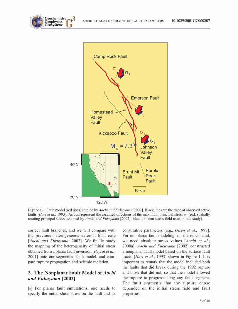
2000a]. Aochi and Fukuyama [2002] constructed

a nonplanar fault model based on the surface fault

traces [Hart et al., 1993] shown in Figure 1. It is

important to remark that the model included both

the faults that did break during the 1992 rupture

and those that did not; so that the model allowed

the rupture to progress along any fault segment.

The fault segments that the rupture chose

depended on the initial stress field and fault

properties.

10 km

40 N°

30 N°120 W°

JohnsonValleyFault

Camp Rock Fault

Brunt Mt.Fault

EurekaPeakFault

HomesteadValleyFault

Kickapoo Fault

Emerson Fault

7.3wM =

1s

1s

1s

1s

Figure 1. Fault model (red lines) studied by Aochi and Fukuyama [2002]. Black lines are the trace of observed activefaults [Hart et al., 1993]. Arrows represent the assumed directions of the maximum principal stress s1 (red, spatiallyrotating principal stress assumed by Aochi and Fukuyama [2002]; blue, uniform stress field used in this study).

GeochemistryGeophysicsGeosystems G3G3 10.1029/2001GC000207aochi et al.: constraint of fault parameters 10.1029/2001GC000207

3 of 16

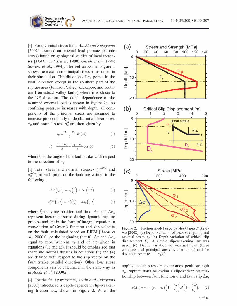
[7] For the initial stress field, Aochi and Fukuyama

[2002] assumed an external load (remote tectonic

stress) based on geological studies of local tecton-

ics [Dokka and Travis, 1990; Unruh et al., 1994;

Sowers et al., 1994]. The red arrows in Figure 1

shows the maximum principal stress s1 assumed in

their simulation. The direction of s1 points in the

NNE direction except in the southern part of the

rupture area (Johnson Valley, Kickapoo, and south-

ern Homestead Valley faults) where it is closer to

the NE direction. The depth dependence of the

assumed external load is shown in Figure 2c. As

confining pressure increases with depth, all com-

ponents of the principal stress are assumed to

increase proportionally to depth. Initial shear stress

t0 and normal stress sn0 are then given by

t0 ¼s1 � s3

2sinð2qÞ ð1Þ

s0n ¼s1 þ s3

2� s1 � s3

2cosð2qÞ ð2Þ

where q is the angle of the fault strike with respect

to the direction of s1.

[8] Total shear and normal stresses (ttotal and

sntotal) at each point on the fault are written in the

following,

ttotal ~x; t� �

¼ t0 ~x� �

þ Dt ~x; t� �

ð3Þ

stotaln~x; t� �

¼ s0n ~x� �

þ Dsn ~x; t� �

ð4Þ

where ~x and t are position and time. Dt and Dsnrepresent increment stress during dynamic rupture

process and are in the form of integral equation, a

convolution of Green’s function and slip velocity

on the fault, calculated based on BIEM [Aochi et

al., 2000a]. At the beginning (t = 0), Dt and Dsnequal to zero, whereas t0 and sn

0 are given in

equations (1) and (2). It should be emphasized that

share and normal stresses in equations (3) and (4)

are defined with respect to the slip vector on the

fault (strike parallel direction). Other four stress

components can be calculated in the same way as

in Aochi et al. [2000a].

[9] For the fault parameters, Aochi and Fukuyama

[2002] introduced a depth-dependent slip-weaken-

ing friction law, shown in Figure 2. When the

applied shear stress t overcomes peak strength

sp, rupture starts following a slip-weakening rela-

tionship between fault function s and fault slip Du,

sðDuÞ¼tr þ sp � tr� �

1� Du

Dc

� �H 1� Du

Dc

� �: ð5Þ

0

10

20

0 20 40 60 80 100 120 140

0

10

20

0 1 2 3 4 5

rt

cD

ps

shear stress

slip

btD

cD

rt0t

ps

(a)

(b)

1s

2s

3s

sD

(c)

0

10

20

0 200 400 600Stress [MPa]

Dep

th [k

m]

Stress and Strength [MPa]

Critical Slip Displacement [m]

Dep

th [k

m]

Dep

th [k

m]

Figure 2. Friction model used by Aochi and Fukuya-ma [2002]. (a) Depth variation of peak strength sp andresidual stress tr. (b) Depth variation of critical slipdisplacement Dc. A simple slip-weakening law wasused. (c) Depth variation of external load (threecompressional principal stress s1 > s2 > s3) and thedeviation Dt = (s1 � s3)/2.



4 of 16

Here tr is residual strength and Dc is critical slip-

weakening distance. Breakdown strength drop Dtbis defined by (sp � tr). H(�) represents the

Heaviside function. The slip-weakening friction

law was proposed theoretically and numerically

[Ida, 1972; Palmer and Rice, 1973], it was then

experimentally observed [Okubo and Dieterich,

1984; Ohnaka et al., 1987], modeled theoretically

[Matsu’ura et al., 1992], and inferred from

seismological modeling of actual earthquake rup-

tures [Ide and Takeo, 1997; Olsen et al., 1997;

Guatteri and Spudich, 2000]. As clearly seen in the

definition of equation (3), this criterion is basically

combined with total shear stress ttotal in equation

(5). In our previous paper [Aochi and Fukuyama,

2002] and this study, all parameters, tr, sp and Dc,

are supposed to be temporally invariable, so that it

is enough to follow numerically shear stress

increment Dt for practical use. On the other hand,

it is possible to introduce a much more complex

criterion instead of equation (5). Aochi et al. [2002]

investigated a dynamic Coulomb law, whose

parameters are temporally variable according to

normal stress increment Dsn. In that case, equation

(5) must be combined with both equations (3) and

(4) at the same time. However, they reported that

increment in normal stress Dsn is generally much

smaller than its absolute normal stress level (sn0)

when we consider a realistic situation of high

confining pressure in the crust, and that, as a result,

the frictional parameters do not change drastically

with time. That is why, in this paper, we will

suppose each frictional parameters are temporally

invariable, and consider the effect of their spatial

heterogeneity on rupture process.

[10] The product of Dtb and Dc determine the

fracture energy, a parameter that is the easiest to

invert from seismic observations [Aki, 1979; Guat-

teri and Spudich, 2000; Peyrat et al., 2002]. The

absolute level of stress in the friction law, sp and

tr, are very important because, for an assumed

external load (remote tectonic stress), we need the

absolute stress field on any segmented, nonplanar

fault system. However, the estimation of absolute

value of fault parameters is still unsolved. Some

seismological analyses proposed that they are

much lower than that extrapolated from experi-

mental results [Bouchon et al., 1998; Spudich et

al., 1998], as well as other geological observation

also suggested low stress along the San Andreas

fault. Regardless of the uncertainty, the depth

variation of the frictional parameters is often used

in the simulation, based on the rheology due to the

pressure and temperature with depth, as modeled in

Sibson [1982], Scholz [1988] and Yamashita and

Ohnaka [1992]. Above the depth of 12 km, the

peak strength sp as a function of depth z is given

by

spðzÞ ¼ s0 þ mf � ðPðzÞ � PH ðzÞÞ; ð6Þ

where mf is frictional coefficient, P and PH are the

confining pressure and hydrostatic pressure, re-

spectively. s0 is the cohesive force, but s0 = 0 was

assumed in the simulation by Aochi and Fukuyama

[2002].

[11] Aochi and Fukuyama [2002] modeled the

rupture process of the Landers earthquake using a

numerical boundary integral equation method

(BIEM) for nonplanar faults embedded in a 3D

unbounded, homogeneous elastic medium [Aochi et

al., 2000a]. Time step and square grid size were

taken as 0.06 s and 750 m, respectively; and P- and

S-wave velocities were 6.20 and 3.52 km/s, respec-

tively. We used mirror sources for approximating

the effect of the free surface. A calculation of 400

time steps took about 4� 105 s of CPU time using 8

to 16 CPUs with fortran90 and MPI on a COMPAQ

ES40 Cluster (EV6 500 MHz), although we occa-

sionally ran several jobs for one simulation.

[12] In Animation 1 (available in the HTML ver-

sion of the article at http://www.g-cubed.org) and

Figure A1a, we show a movie of one of the

dynamic simulations by Aochi and Fukuyama

[2002]. We observe that rupture does not propagate

on the northern Johnson Valley fault, but chooses

the Kickapoo and Homestead Valley faults instead,

and then jumps to the northernmost Camp Rock

fault. This is the most important feature of the

Landers earthquake that they succeeded in repro-

ducing. In the following sections, we will inves-

tigate how important were the assumptions they

made for rupture propagation, and then discuss



5 of 16

how we may constrain the fault properties from the

numerical simulations.

3. Constraint of the Depth-DependentFriction Law

[13] Although the segmented model of Aochi and

Fukuyama [2002] reproduced the general features

of rupture propagation along the fault system, there

are some clear discrepancies between their model

and observations. In their simulations, there were

several large slip areas along strike in overall

agreement with the asperities inferred from kine-

matic inversion [Wald and Heaton, 1994], but the

maximum slip was located at a depth of around

12 km. Thus, their model could not produce large

slip near the ground surface, although a slip of

more than 5 m was observed in the field [Hart et

al., 1993]. The discrepancy is due to the depth

dependency of friction assumed in the simulation,

the depth of 12 km corresponds to the depth where

the breakdown strength drop is maximum, as

shown in Figure 2. Clearly the assumption of zero

peak strength at the ground surface is incorrect.

Thus, we have to modify the depth variation of

fault properties adapting finite cohesive force s0 inequation (6), so that we expect that finite stress

could be accumulated and released near the ground

surface to produce much fault slip.

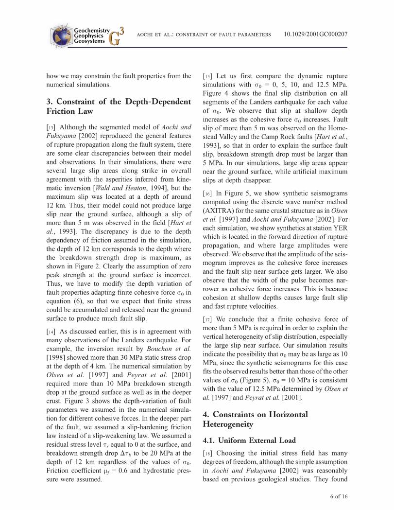
[14] As discussed earlier, this is in agreement with

many observations of the Landers earthquake. For

example, the inversion result by Bouchon et al.

[1998] showed more than 30 MPa static stress drop

at the depth of 4 km. The numerical simulation by

Olsen et al. [1997] and Peyrat et al. [2001]

required more than 10 MPa breakdown strength

drop at the ground surface as well as in the deeper

crust. Figure 3 shows the depth-variation of fault

parameters we assumed in the numerical simula-

tion for different cohesive forces. In the deeper part

of the fault, we assumed a slip-hardening friction

law instead of a slip-weakening law. We assumed a

residual stress level tr equal to 0 at the surface, and

breakdown strength drop Dtb to be 20 MPa at the

depth of 12 km regardless of the values of s0.Friction coefficient mf = 0.6 and hydrostatic pres-

sure were assumed.

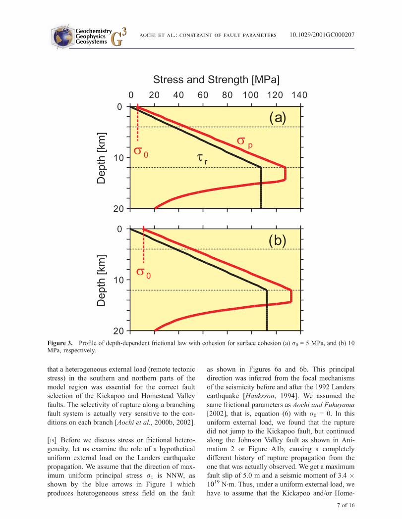
[15] Let us first compare the dynamic rupture

simulations with s0 = 0, 5, 10, and 12.5 MPa.

Figure 4 shows the final slip distribution on all

segments of the Landers earthquake for each value

of s0. We observe that slip at shallow depth

increases as the cohesive force s0 increases. Faultslip of more than 5 m was observed on the Home-

stead Valley and the Camp Rock faults [Hart et al.,

1993], so that in order to explain the surface fault

slip, breakdown strength drop must be larger than

5 MPa. In our simulations, large slip areas appear

near the ground surface, while artificial maximum

slips at depth disappear.

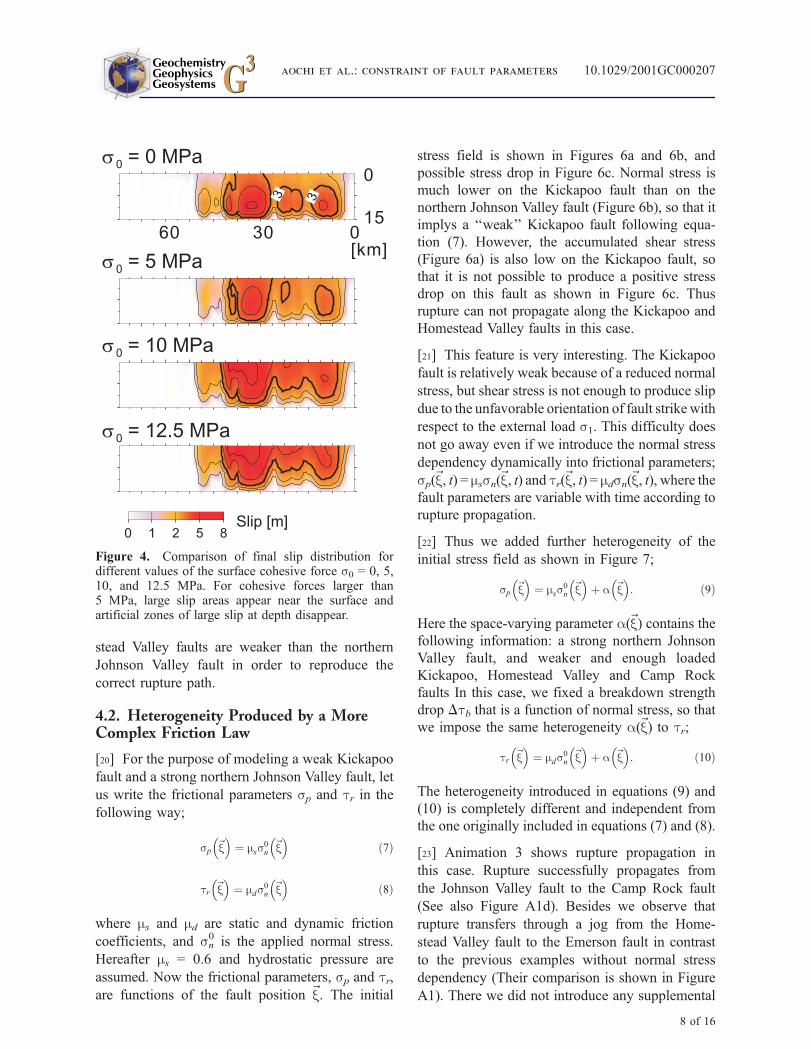
[16] In Figure 5, we show synthetic seismograms

computed using the discrete wave number method

(AXITRA) for the same crustal structure as inOlsen

et al. [1997] and Aochi and Fukuyama [2002]. For

each simulation, we show synthetics at station YER

which is located in the forward direction of rupture

propagation, and where large amplitudes were

observed. We observe that the amplitude of the seis-

mogram improves as the cohesive force increases

and the fault slip near surface gets larger. We also

observe that the width of the pulse becomes nar-

rower as cohesive force increases. This is because

cohesion at shallow depths causes large fault slip

and fast rupture velocities.

[17] We conclude that a finite cohesive force of

more than 5 MPa is required in order to explain the

vertical heterogeneity of slip distribution, especially

the large slip near surface. Our simulation results

indicate the possibility that s0 may be as large as 10

MPa, since the synthetic seismograms for this case

fits the observed results better than those of the other

values of s0 (Figure 5). s0 = 10 MPa is consistent

with the value of 12.5 MPa determined by Olsen et

al. [1997] and Peyrat et al. [2001].

4. Constraints on HorizontalHeterogeneity

4.1. Uniform External Load

[18] Choosing the initial stress field has many

degrees of freedom, although the simple assumption

in Aochi and Fukuyama [2002] was reasonably

based on previous geological studies. They found



6 of 16

that a heterogeneous external load (remote tectonic

stress) in the southern and northern parts of the

model region was essential for the correct fault

selection of the Kickapoo and Homestead Valley

faults. The selectivity of rupture along a branching

fault system is actually very sensitive to the con-

ditions on each branch [Aochi et al., 2000b, 2002].

[19] Before we discuss stress or frictional hetero-

geneity, let us examine the role of a hypothetical

uniform external load on the Landers earthquake

propagation. We assume that the direction of max-

imum uniform principal stress s1 is NNW, as

shown by the blue arrows in Figure 1 which

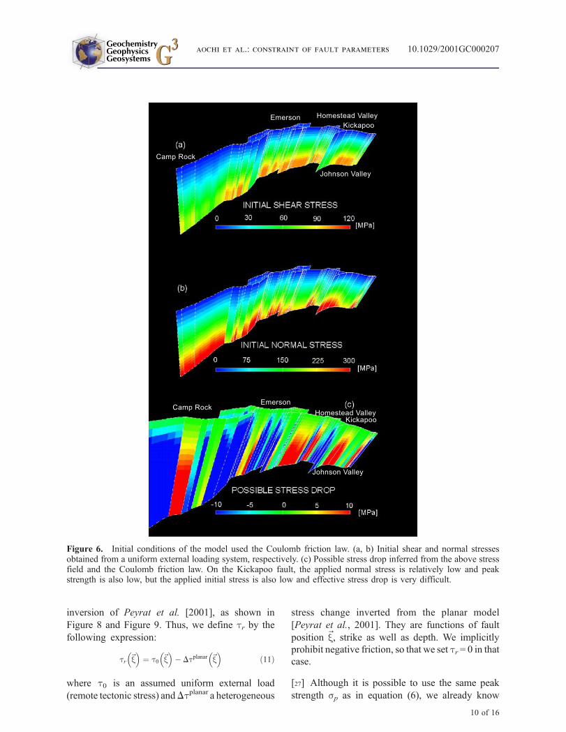
produces heterogeneous stress field on the fault

as shown in Figures 6a and 6b. This principal

direction was inferred from the focal mechanisms

of the seismicity before and after the 1992 Landers

earthquake [Hauksson, 1994]. We assumed the

same frictional parameters as Aochi and Fukuyama

[2002], that is, equation (6) with s0 = 0. In this

uniform external load, we found that the rupture

did not jump to the Kickapoo fault, but continued

along the Johnson Valley fault as shown in Ani-

mation 2 or Figure A1b, causing a completely

different history of rupture propagation from the

one that was actually observed. We get a maximum

fault slip of 5.0 m and a seismic moment of 3.4 �1019 N�m. Thus, under a uniform external load, we

have to assume that the Kickapoo and/or Home-

0

10

20

Dep

th [k

m]

0 20 40 60 80 100 120 140

Stress and Strength [MPa]

0

10

20

rt

(a)

(b)

ps

0s

0s

Dep

th [k

m]

Figure 3. Profile of depth-dependent frictional law with cohesion for surface cohesion (a) s0 = 5 MPa, and (b) 10MPa, respectively.



7 of 16

stead Valley faults are weaker than the northern

Johnson Valley fault in order to reproduce the

correct rupture path.

4.2. Heterogeneity Produced by a MoreComplex Friction Law

[20] For the purpose of modeling a weak Kickapoo

fault and a strong northern Johnson Valley fault, let

us write the frictional parameters sp and tr in the

following way;

sp ~x� �

¼ mss0n~x� �

ð7Þ

tr ~x� �

¼ mds0n~x� �

ð8Þ

where ms and md are static and dynamic friction

coefficients, and sn0 is the applied normal stress.

Hereafter ms = 0.6 and hydrostatic pressure are

assumed. Now the frictional parameters, sp and tr,are functions of the fault position ~x. The initial

stress field is shown in Figures 6a and 6b, and

possible stress drop in Figure 6c. Normal stress is

much lower on the Kickapoo fault than on the

northern Johnson Valley fault (Figure 6b), so that it

implys a ‘‘weak’’ Kickapoo fault following equa-

tion (7). However, the accumulated shear stress

(Figure 6a) is also low on the Kickapoo fault, so

that it is not possible to produce a positive stress

drop on this fault as shown in Figure 6c. Thus

rupture can not propagate along the Kickapoo and

Homestead Valley faults in this case.

[21] This feature is very interesting. The Kickapoo

fault is relatively weak because of a reduced normal

stress, but shear stress is not enough to produce slip

due to the unfavorable orientation of fault strike with

respect to the external load s1. This difficulty does

not go away even if we introduce the normal stress

dependency dynamically into frictional parameters;

sp(~x, t) = mssn(~x, t) and tr(~x, t) = mdsn(~x, t), where thefault parameters are variable with time according to

rupture propagation.

[22] Thus we added further heterogeneity of the

initial stress field as shown in Figure 7;

sp ~x� �

¼ mss0n~x� �

þ a ~x� �

: ð9Þ

Here the space-varying parameter a(~x) contains thefollowing information: a strong northern Johnson

Valley fault, and weaker and enough loaded

Kickapoo, Homestead Valley and Camp Rock

faults In this case, we fixed a breakdown strength

drop Dtb that is a function of normal stress, so that

we impose the same heterogeneity a(~x) to tr;

tr ~x� �

¼ mds0n~x� �

þ a ~x� �

: ð10Þ

The heterogeneity introduced in equations (9) and

(10) is completely different and independent from

the one originally included in equations (7) and (8).

[23] Animation 3 shows rupture propagation in

this case. Rupture successfully propagates from

the Johnson Valley fault to the Camp Rock fault

(See also Figure A1d). Besides we observe that

rupture transfers through a jog from the Home-

stead Valley fault to the Emerson fault in contrast

to the previous examples without normal stress

dependency (Their comparison is shown in Figure

A1). There we did not introduce any supplemental

3 3

0 1 2 5 8Slip [m]

15

0

03060[km]

0s = 0 MPa

0s = 5 MPa

0s = 12.5 MPa

0s = 10 MPa

Figure 4. Comparison of final slip distribution fordifferent values of the surface cohesive force s0 = 0, 5,10, and 12.5 MPa. For cohesive forces larger than5 MPa, large slip areas appear near the surface andartificial zones of large slip at depth disappear.



8 of 16

heterogeneity. As a result, we get a maximum fault

slip of 3.67 m and a seismic moment of 5.2 � 1019

N � s.

[24] In conclusion, in order to reproduce the rup-

ture transfer between different fault branches,

especially from the Johnson Valley to the Kickapoo

and Homestead Valley faults, we needed an addi-

tional heterogeneity a(~x) which explicitly indicates

a weak Kickapoo fault and a strong northern

Johnson Valley fault. This seems to be very

unlikely. Rockwell et al. [2000] investigated paleo-

seismic data from several trenches and reported

that the time intervals from previous event for the

southern and northern Johnson Valley and Kick-

apoo faults were about 5000 years, while those of

the Homestead Valley, Emerson and Camp Rock

faults were more than 7000 years.

4.3. Stress Heterogeneity Derived FromPlanar-Fault Simulations

[25] Olsen et al. [1997] and Peyrat et al. [2001,

2002] successfully determined the heterogeneous

initial stress field of the Landers earthquake for a

single planar fault through the inversion of the

observed ground motion. Since they assumed a

single planar fault, the heterogeneity of the stress

field can be transferred into the heterogeneity of

frictional parameters as long as the amount of

available energy to fracture energy is the same in

the two models [Peyrat et al., 2002]. That is, a

certain relation between t0, sp and tr, that is

required stress excess Dteplanar (� sp � t0) and

possible stress drop Dtplanar (� t0 � tr) is

conserved. In the following, we consider how to

map their heterogeneity into our nonplanar fault

modeling.

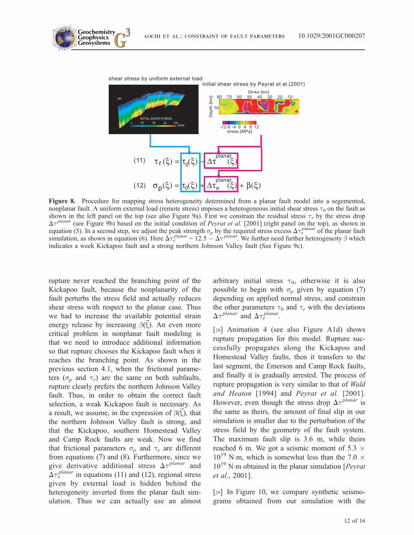
[26] Figure 8 briefly shows the procedure we

propose in this section. We start with the uniform

external load (remote tectonic stress) as assumed

in section 4.1, and indicated by the blue allows

in Figure 1. For the purpose of determining the

final slip distribution during the earthquake, static

stress drop plays a fundamental role. We assume

possible stress drop Dt based on the planar-fault

20 cm

20s

E

W

N

S

U

D

obs.

YER

0 12.5MPas =0 5MPas =0 0MPas = 0 10MPas =

30 kmYER

Figure 5. Comparison of synthetic seismogram at the YER station for each simulation shown in Figure 4. Ascohesive force increases, the amplitude of synthetic seismograms improves. Seismograms are zero-phrase bandpassfiltered between 0.07 and 0.5 Hz.



9 of 16

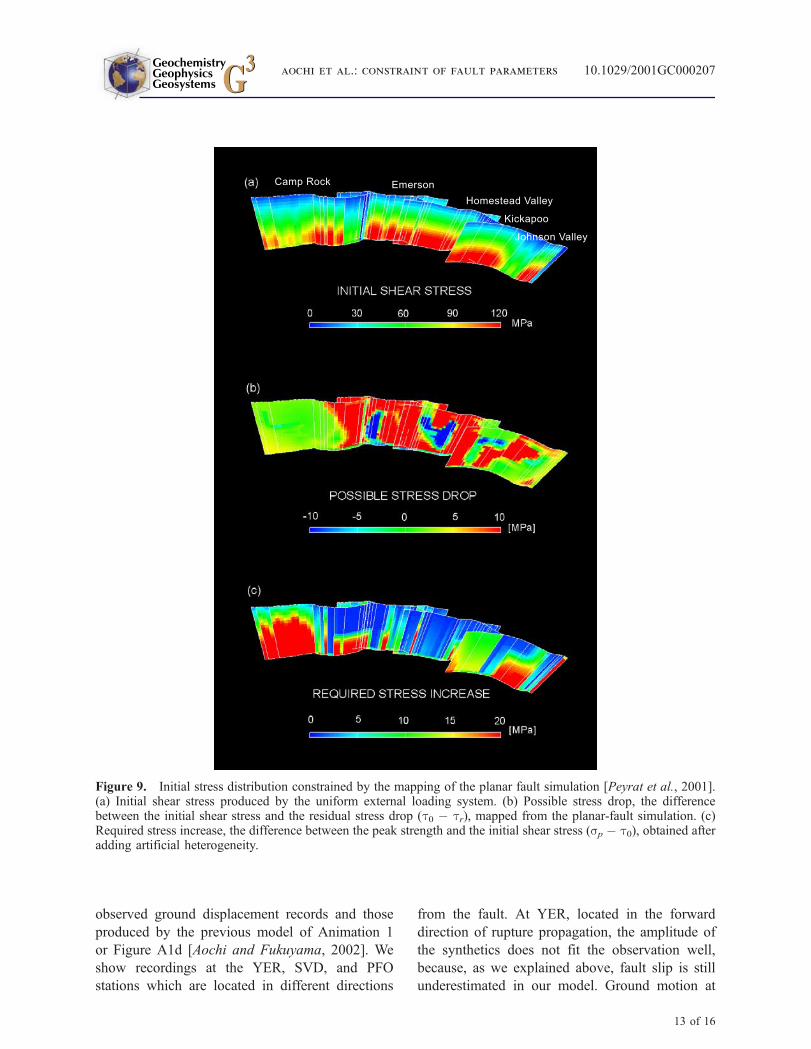
inversion of Peyrat et al. [2001], as shown in

Figure 8 and Figure 9. Thus, we define tr by the

following expression:

tr ~x� �

¼ t0 ~x� �

� Dtplanar ~x� �

ð11Þ

where t0 is an assumed uniform external load

(remote tectonic stress) andDtplanar a heterogeneous

stress change inverted from the planar model

[Peyrat et al., 2001]. They are functions of fault

position ~x, strike as well as depth. We implicitly

prohibit negative friction, so that we set tr = 0 in thatcase.

[27] Although it is possible to use the same peak

strength sp as in equation (6), we already know

Johnson Valley

Emerson

Camp Rock

Homestead ValleyKickapoo

Johnson Valley

EmersonCamp Rock

Homestead ValleyKickapoo

Figure 6. Initial conditions of the model used the Coulomb friction law. (a, b) Initial shear and normal stressesobtained from a uniform external loading system, respectively. (c) Possible stress drop inferred from the above stressfield and the Coulomb friction law. On the Kickapoo fault, the applied normal stress is relatively low and peakstrength is also low, but the applied initial stress is also low and effective stress drop is very difficult.



10 of 16

that this did not work in the case of the uniform

external load. Thus, in order for rupture to progress

correctly, we also have to change peak strength

sp – or strictly speaking, the stress increase (Dte)from the assumed initial stress field (sp � t0).Actually, we not only give the stress increase

Dteplanar of the planar fault simulation [Peyrat et

al., 2001], but also a small additional heterogeneity

b(~x).

sp ~x� �

¼ t0 ~x� �

þ Dtplanare~x� �

þ b ~x� �

ð12Þ

That is necessary because, without a small b(~x), therupture does not propagate. In the simulations the

Johnson Valley

Emerson

Camp Rock

Homestead Valley

Kickapoo

Figure 7. Initial conditions with additional heterogeneity to that in Figure 6. (a) Required stress increase, and (b)possible stress drop. Artificial heterogeneity is given independently from the Coulomb friction law. In this case, theKickapoo fault is weak enough compared to the applied initial shear stress.



11 of 16

rupture never reached the branching point of the

Kickapoo fault, because the nonplanarity of the

fault perturbs the stress field and actually reduces

shear stress with respect to the planar case. Thus

we had to increase the available potential strain

energy release by increasing b(~x). An even more

critical problem in nonplanar fault modeling is

that we need to introduce additional information

so that rupture chooses the Kickapoo fault when it

reaches the branching point. As shown in the

previous section 4.1, when the frictional parame-

ters (sp and tr) are the same on both subfaults,

rupture clearly prefers the northern Johnson Valley

fault. Thus, in order to obtain the correct fault

selection, a weak Kickapoo fault is necessary. As

a result, we assume, in the expression of b(~x), thatthe northern Johnson Valley fault is strong, and

that the Kickapoo, southern Homestead Valley

and Camp Rock faults are weak. Now we find

that frictional parameters sp and tr are different

from equations (7) and (8). Furthermore, since we

give derivative additional stress Dtplanar and

Dteplanar in equations (11) and (12), regional stress

given by external load is hidden behind the

heterogeneity inverted from the planar fault sim-

ulation. Thus we can actually use an almost

arbitrary initial stress t0, otherwise it is also

possible to begin with sp given by equation (7)

depending on applied normal stress, and constrain

the other parameters t0 and tr with the deviations

Dtplanar and Dteplanar.

[28] Animation 4 (see also Figure A1d) shows

rupture propagation for this model. Rupture suc-

cessfully propagates along the Kickapoo and

Homestead Valley faults, then it transfers to the

last segment, the Emerson and Camp Rock faults,

and finally it is gradually arrested. The process of

rupture propagation is very similar to that of Wald

and Heaton [1994] and Peyrat et al. [2001].

However, even though the stress drop Dtplanar is

the same as theirs, the amount of final slip in our

simulation is smaller due to the perturbation of the

stress field by the geometry of the fault system.

The maximum fault slip is 3.6 m, while theirs

reached 6 m. We got a seismic moment of 5.3 �1019 N�m, which is somewhat less than the 7.0 �1019 N�m obtained in the planar simulation [Peyrat

et al., 2001].

[29] In Figure 10, we compare synthetic seismo-

grams obtained from our simulation with the

10

Dep

th [

km] 80 70 60 50 40 30 20 10

Strike [km]

-12-8 -4 0 4 8 12stress [MPa]

shear stress by uniform external loadinitial shear stress by Peyrat et al.(2001)

(11)

(12)

τ (ξ) = τ (ξ) − ∆τ (ξ)r 0

planar

σ (ξ) = τ (ξ) + ∆τ (ξ) + β(ξ)0

planar

ep

Figure 8. Procedure for mapping stress heterogeneity determined from a planar fault model into a segemented,nonplanar fault. A uniform external load (remote stress) imposes a heterogeneous initial shear stress t0 on the fault asshown in the left panel on the top (see also Figure 9a). First we constrain the residual stress tr by the stress dropDtplanar (see Figure 9b) based on the initial condition of Peyrat et al. [2001] (right panel on the top), as shown inequation (5). In a second step, we adjust the peak strength sp by the required stress excess Dte

planar of the planar faultsimulation, as shown in equation (6). Here Dte

planar = 12.5 � Dtplanar. We further need further heterogeneity b whichindicates a week Kickapoo fault and a strong northern Johnson Valley fault (See Figure 9c).



12 of 16

observed ground displacement records and those

produced by the previous model of Animation 1

or Figure A1d [Aochi and Fukuyama, 2002]. We

show recordings at the YER, SVD, and PFO

stations which are located in different directions

from the fault. At YER, located in the forward

direction of rupture propagation, the amplitude of

the synthetics does not fit the observation well,

because, as we explained above, fault slip is still

underestimated in our model. Ground motion at

Johnson Valley

EmersonCamp Rock

Homestead Valley

Kickapoo

Figure 9. Initial stress distribution constrained by the mapping of the planar fault simulation [Peyrat et al., 2001].(a) Initial shear stress produced by the uniform external loading system. (b) Possible stress drop, the differencebetween the initial shear stress and the residual stress drop (t0 � tr), mapped from the planar-fault simulation. (c)Required stress increase, the difference between the peak strength and the initial shear stress (sp � t0), obtained afteradding artificial heterogeneity.



13 of 16

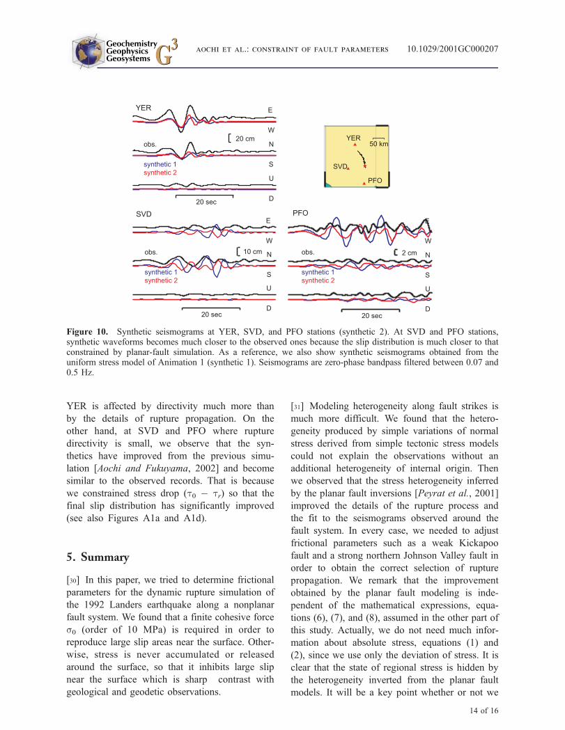
YER is affected by directivity much more than

by the details of rupture propagation. On the

other hand, at SVD and PFO where rupture

directivity is small, we observe that the syn-

thetics have improved from the previous simu-

lation [Aochi and Fukuyama, 2002] and become

similar to the observed records. That is because

we constrained stress drop (t0 � tr) so that the

final slip distribution has significantly improved

(see also Figures A1a and A1d).

5. Summary

[30] In this paper, we tried to determine frictional

parameters for the dynamic rupture simulation of

the 1992 Landers earthquake along a nonplanar

fault system. We found that a finite cohesive force

s0 (order of 10 MPa) is required in order to

reproduce large slip areas near the surface. Other-

wise, stress is never accumulated or released

around the surface, so that it inhibits large slip

near the surface which is sharp contrast with

geological and geodetic observations.

[31] Modeling heterogeneity along fault strikes is

much more difficult. We found that the hetero-

geneity produced by simple variations of normal

stress derived from simple tectonic stress models

could not explain the observations without an

additional heterogeneity of internal origin. Then

we observed that the stress heterogeneity inferred

by the planar fault inversions [Peyrat et al., 2001]

improved the details of the rupture process and

the fit to the seismograms observed around the

fault system. In every case, we needed to adjust

frictional parameters such as a weak Kickapoo

fault and a strong northern Johnson Valley fault in

order to obtain the correct selection of rupture

propagation. We remark that the improvement

obtained by the planar fault modeling is inde-

pendent of the mathematical expressions, equa-

tions (6), (7), and (8), assumed in the other part of

this study. Actually, we do not need much infor-

mation about absolute stress, equations (1) and

(2), since we use only the deviation of stress. It is

clear that the state of regional stress is hidden by

the heterogeneity inverted from the planar fault

models. It will be a key point whether or not we

E

W

N

S

U

D

SVDE

W

N

S

U

D

20 cm

20 sec

E

W

N

S

U

D

obs.

YER

synthetic 1synthetic 2

50 kmYER

SVD

PFO

PFO

10 cm

20 sec

obs.


obs.


2 cm

20 sec

Figure 10. Synthetic seismograms at YER, SVD, and PFO stations (synthetic 2). At SVD and PFO stations,synthetic waveforms becomes much closer to the observed ones because the slip distribution is much closer to thatconstrained by planar-fault simulation. As a reference, we also show synthetic seismograms obtained from theuniform stress model of Animation 1 (synthetic 1). Seismograms are zero-phase bandpass filtered between 0.07 and0.5 Hz.



14 of 16

can find this kind of information for realistic

rupture models.

Appendix: Snapshots of DynamicSimulation

[32] Simulation results are given as movie files in

this manuscript. In Figure A1, we further show

their snapshots in static images for convenience.

Acknowledgments

[33] We would like to thank Ruth Harris, an anonymous

reviewer and Rick O’Connell whose comments help us to

improve this manuscript. For numerical simulations, we used

the parallel computer at the Departement de Simulation

Physique et Numerique de l’Institut de Physique du Globe

de Paris (IPGP). This research was supported by the profect

‘‘Rupture et changement d’echelle’’ of ACI Catastrophes

Naturelles of the Ministere de la Recherche, France.

References

Aki, K., Characterization of barriers of an earthquake fault,

J. Geophys. Res., 84, 6140–6148, 1979.

Aochi, H., and E. Fukuyama, Three-dimensional nonplanar

simulation of the 1992 Landers earthquake, J. Geophys.

Res., 107(B2), 2035, doi:10.1029/2000JB000061, 2002.

Aochi, H., E. Fukuyama, and M. Matsu’ura, Spontaneous

Rupture Propagation on a Non-planar Fault in 3-D Elastic

Medium, PAGEOPH, 157, 2003–2027, 2000a.

Aochi, H., E. Fukuyama, and M. Matsu’ura, Selectivity of

spontaneous rupture propagation on a branched fault, Geo-

phys. Res. Lett., 27, 3635–3638, 2000b.

Aochi, H., R. Madariaga, and E. Fukuyama, Effect of nor-

mal stress during rupture propagation along nonplanar

faults, J. Geophys. Res., 107(B2), 2038, doi:10.1029/

2001JB000500, 2002.

Boatwright, J., and M. Cocco, Frictional constraints on crustal

faulting, J. Geophys. Res., 101, 13,895–13,909, 1996.

Bouchon, M., M. Campillo, and F. Cotton, Stress field asso-

ciated with the rupture of the 1992 Landers, California,

earthquake and its implications concerning the fault strength

at the onset of the earthquake, J. Geophys. Res., 103,

21,091–21,097, 1998a.

Bouchon, M., H. Sekiguchi, K. Irikura, and T. Iwata, Some

characteristics of the stress field of the 1995 Hyogo-ken

Nanbu (Kobe) earthquake, J. Geophys. Res., 103, 24,271–

24,282, 1998b.

Cochard, A., and R. Madariaga, Dynamic faulting under rate-

dependent friction, PAGEOPH, 142, 419–445, 1994.

Day, S., G. Yu, and D. J. Wald, Dynamic stress changes during

earthquake rupture, Bull. Seismol. Soc. Am., 88, 512–522,

1998.

Dokka, R. K., and C. J. Travis, Role of the eastern California

shear zone in accommodating Pacific-North American plate

motion, Geophys. Res. Lett., 17, 1323–1326, 1990.

Fukuyama, E., and R. Madariaga, Integral equation method for

plane crack with arbitrary shape in 3d elastic medium, Bull.

Seismol. Soc. Am., 85, 614–628, 1995.

Guatteri, M., and P. Spudich, What can strong-motion data tell

us about slip-weakening fault-friction laws?, Bull. Seismol.

Soc. Am., 90, 98–116, 2000.

Guatteri, M., G. Beroza, and P. Spudich, Inferring rate and

state friction parameters from a rupture model of the 1995

Hyogo-ken Nanbu (Kobe) Japan earthquake, J. Geophys.

Res., 106, 26,511–26,522, 2001.

EmersonCamp Rock

Homestead Valley

t=2 s

9 s

16 s

23 s

(a) (b) (c) (d)

Fault Slip [m]

0 51 2 3 4

0

15 km

Kickapoo

Johnson Valley

Figure A1. Snapshots of each simulation shown in this study. (a) The previous simulations of Aochi and Fukuyama[2002]. Its movie is in Animation 1. (b) The case of uniform loading stress (Animation 2). Rupture propagates on theJohnson Valley fault. (c) The model including applied normal stress in frictional parameters (Animation 3). (d) Themodel with initial condition similar to that of the planar fault simulation (Animation 4).



15 of 16

Harris, R. A., and S. M. Day, Dynamics of fault interaction:

Parallel strike-slip faults, Geophys. Res. Lett., 98, 4461–

4472, 1993.

Harris, R. A., and S. M. Day, Dynamic 3D simulations of

earthquakes on en echelon faults, Geophys. Res. Lett., 26,

2089–2092, 1999.

Harris, R. A., R. J. Archuleta, and S. M. Day, Fault step and

the dynamic rupture process: 2-D numerical simulations of a

spontaneously propagating shear fracture, Geophys. Res.

Lett., 18, 893–896, 1991.

Hart, E. W., W. A. Bryant, and J. A. Treiman, Surface faulting

associated with the June 1992 Landers earthquake, Califor-

nia, Calif. Geol., 46, 10–16, 1993.

Hauksson, E., State of stress from focal mechanisms before

and after the 1992 Landers earthquake sequence, Bull. Seis-

mol. Soc. Am., 84, 917–934, 1994.

Ida, Y., Cohesive force across the tip of a longitudinal-shear

crack and Griffith’s specific surface energy, J. Geophys. Res.,

77, 3796–3805, 1972.

Ide, S., and M. Takeo, Determination of constitutive relations

of fault slip based on seismic wave analysis, J. Geophys.

Res., 102, 27,379–27,391, 1997.

Kame, N., and T. Yamashita, Dynamic nucleation process of

shallow earthquake faulting in a fault zone, Geophys. J. Int.,

128, 204–216, 1997.

Kame, N., and T. Yamashita, Simulation of the spontaneous

growth of a dynamic crack without constraints on the crack

tip path, Geophys. J. Int., 139, 345–358, 1999.

Kase, Y., and K. Kuge, Numerical simulation of spontaneous

rupture processes on two non-coplanar faults: The effect of

geometry on fault interaction, Geophys. J. Int., 135, 911–

922, 1998.

Kase, Y., and K. Kuge, Rupture propagation beyond fault dis-

continuities: Significance of fault strike and location, Geo-

phys. J. Int., 147, 330–342, 2001.

Koller, M. G., M. Bonnet, and R. Madariaga, Modeling of

dynamical crack propagation using time-domain boundary

integral equations, Wave Motion, 16, 339–366, 1992.

Madariaga, R., On the relation between seismic moment and

stress drop in the presence of stress and strength heteroge-

neity, J. Geophys. Res., 84, 2243–2250, 1979.

Matsu’ura, M., H. Kataoka, and B. Shibazaki, Slip-dependent

friction law and nucleation processes in earthquake rupture,

Tectonophysics, 211, 135–148, 1992.

Okubo, P. G., and J. H. Dieterich, Effects of physical fault

properties on frictional instabilities produced on simulated

faults, J. Geophys. Res., 89, 5817–5827, 1984.

Ohnaka, M., Y. Kuwahara, and K. Yamamoto, Constitutive

relations between dynamic physical parameters near a tip

of the propagating slip zone during stick-slip shear failure,

Tectonophys., 144, 109–125, 1987.

Olsen, K. B., R. Madariaga, and R. J. Archuleta, Three-Dimen-

sional dynamic simulation of the 1992 Landers Earthquake,

Science, 278, 834–838, 1997.

Palmer, A. C., and J. R. Rice, The growth of slip surfaces in

the progressive failure of over-consolidated clay, Proc. R.

Soc. London Ser. A, 332, 527–548, 1973.

Peyrat, S., K. B. Olsen, and R. Madariaga, Dynamic modeling

of the 1992 Landers Earthquake, J. Geophys. Res., 106,

26,467–26,482, 2001.

Peyrat, S., K. B. Olsen, and R. Madariaga, La dynamique des

tremblements de terre vue a travers le seisme de Landers du

28 Juin 1992, C. R. Acad. Sci. Paris, 330, 235–248, 2002.

Rockwell, T. K., S. Lindvall, M. Herzberg, D. Murbach,

T. Dawson, and G. Berger, Paleoseismology of the Johnson

Valley, Kickapoo, and Homestead Valley Faults: Clustering

of earthquakes in the eastern California shear zone, Bull.

Seismol. Soc. Am., 90, 1200–1236, 2000.

Scholz, C. H., The brittle-plastic transition and the depth of

seismic faulting, Geol. Rund., 77, 319–328, 1988.

Sibson, R. H., Fault zone models, heat flow, and the depth

distribution of earthquakes in the continental crust of the

United States, Bull. Seismol. Soc. Am., 72, 151–163, 1982.

Sowers, J. M., J. R. Unruh, W. R. Lettis, and T. D. Rubin,

Relationship of the Kickapoo Fault to the Johnson Valley

and Homestead Valley Faults, San Bernardino Country, Ca-

lifornia, Bull. Seismol. Soc. Am., 84, 528–536, 1994.

Spudich, P., M. Guatteri, K. Otsuki, and J. Minagawa, Use of

Fault Striations and Dislocation Models to Infer Tectonic

Shear Stress during the 1995 Hyogo-ken Nanbu (Kobe)

Earthquake, J. Geophys. Res., 88, 413–427, 1998.

Tada, T., and T. Yamashita, Non-hypersingular boundary inte-

gral equations for two-dimensional non-planar crack analy-

sis, Geophys. J. Int., 130, 269–282, 1997.

Unruh, J. R., W. R. Lettis, and J. M. Sowers, Kinematic Inter-

pretation of the 1992 Landers Earthquake, Bull. Seismol.

Soc. Am., 84, 537–546, 1994.

Wald, D. J., and T. H. Heaton, Spatial and temporal distribu-

tion of slip for the 1992 Landers, California, earthquake,

Bull. Seismol. Soc. Am., 84, 668–691, 1994.

Yamashita, T., and M. Ohnaka, Precursory surface deformation

expected from a strike-slip fault model into which rheologi-

cal properties of the lithosphere are incorporated, Tectono-

physics, 211, 179–199, 1992.



16 of 16

Geochemistry 3 Volume 4 Geophysics Geosystemsmadariag/Papers/aochig3.pdf · Constraint of fault...

Documents

Transcript of Geochemistry 3 Volume 4 Geophysics Geosystemsmadariag/Papers/aochig3.pdf · Constraint of fault...