RESEARCH ARTICLE

Genetic structure of a montane perennial plant: the influenceof landscape and flowering phenology

Sevan S. Suni1 • Andrew R. Whiteley2

Received: 20 May 2015 / Accepted: 30 June 2015

� Springer Science+Business Media Dordrecht 2015

Abstract The way that genetic variation is distributed

geographically has important conservation and evolution-

ary implications. Here, we examined the distribution of

genetic variation within and among populations of the

montane perennial Ipomopsis aggregata. We sampled

plants in western Colorado and examined (1) population

genetic structure over a geographic area that spanned

130 km, including genetic variation within disturbed and

undisturbed sites; (2) the relationship between genetic

differentiation and geographic distance; and (3) the rela-

tionship between flowering time and genetic differentiation

among plants within and among geographic areas. FIS was

significantly higher (t test, P = 0.006), expected

heterozygosity was significantly lower (t test, P = 0.04),

and allelic richness was marginally significantly lower

(t test, P = 0.078) among anthropogenically-disturbed

sites compared to undisturbed sites. We found moderate

genetic differentiation over the area sampled (average

pairwise FST = 0.04; average pairwise F0ST ¼ 0:19), but no

association of genetic and geographic distance (Mantel test

P values 0.44 for FST and 0.36 for F0ST ). We found a strong

association of flowering time and genetic differentiation

over small and large spatial scales. Genetic differentiation

between early and late flowering plants within a focal site

was statistically significant (genic test for population dif-

ferentiation combined P value\0.001; FST = 0.05). There

was a significant correlation between genetic distance (F0ST )

and distance in flowering time, when controlling for geo-

graphic distance, over the whole geographic area (Partial

Mantel test Rxy = 0.32, P = 0.013). A multiple regression

with randomization further supported the inference that

flowering time, but not geographic distance or elevation,

predicted F0ST (geographic distance: b = -0.03, P = 0.89;

elevation: b = 0.01, P = 0.96; phenological distance:

b = 0.30, P = 0.05), but not FST (geographic distance:

b = -0.02, P = 0.92; elevation: b = 0.14, P = 0.38;

phenological distance: b = 0.25, P = 0.11), unless eleva-

tion was left out of the model (geographic distance:

b = -0.03, P = 0.9; phenological distance: b = 0.29,

P = 0.03). The association of flowering time and genetic

distance despite the lack of isolation by distance provides

further evidence for the usefulness of incorporating this

variable into plant landscape genetic studies when possible.

Keywords Genetic differentiation � Genetic structure �Phenology � Flowering time � Ipomopsis aggregata

Introduction

The way that genetic variation is distributed geographically

has important evolutionary and conservation implications

(Allendorf and Luikart 2007; Frankham 2010). Analyses of

population genetic structure can help identify where con-

nectivity might have been decreased by human activities as

well as reveal small, genetically depauperate populations

that might have elevated probabilities of inbreeding

Data accessibility Microsatellite genotypes will be submitted toDryad Digital Repository for archiving.

Electronic supplementary material The online version of thisarticle (doi:10.1007/s10592-015-0751-z) contains supplementarymaterial, which is available to authorized users.

& Sevan S. Suni

suni@fas.harvard.edu

1 Department of Organismic and Evolutionary Biology,

Harvard University, Boston, MA 02131, USA

2 Department of Environmental Conservation, University of

Massachusetts, Amherst, MA 01003, USA

123

Conserv Genet

DOI 10.1007/s10592-015-0751-z

depression and lower probabilities of persistence (Soule

1987; Gilpin and Hanski 1991; Saccheri et al. 1998). The

geographic distribution of genetic variation within net-

works of connected and locally adapted populations also

shapes the way species respond to environmental changes

(Jay et al. 2012), for example through what has been ter-

med the Portfolio effect in which genetic diversity within

and divergence among connected populations enhances

long-term sustainability of populations experiencing envi-

ronmental changes (Shindler et al. 2010).

The field of landscape genetics combines population

genetics with landscape ecology to explain how landscape

features—such as rivers or mountains—influence the dis-

tribution of genetic variation (Manel et al. 2003; Storfer

et al. 2007; Holderegger and Wagner 2008). In addition to

geographic distance (i.e., isolation by distance, IBD;

Wright 1943) or environmental characteristics such as

elevation or habitat type (i.e., isolation by environment,

IBE; Wang 2013), an important, but less often considered

factor spatially shaping intraspecific genetic structure is the

timing of reproductive events (Stanton et al. 1997).

Reproductive timing determines mate availability, so

individuals that reproduce at more similar times will be

more likely to mate with one another. If a population

contains individuals that reproduce at heritably different

times, genetic differentiation among individuals should be

positively related to increasing differences in reproductive

timing, a phenomenon called ‘isolation by time’ by Hendry

and Day (2005). Hendry and Day (2005) predict that

increasing heritabilities of reproductive time will lead to a

stronger association of differences in reproductive time and

genetic differences. Whether or not reproductive timing is

heritable, it is plausible that individuals could show an

association between phenology and relatedness if repro-

ductive timing is governed by environmental variables that

vary spatially in a consistent manner, and if dispersal is

restricted.

For plants, associations between flowering time and

genetic structure are likely because plants that flower at the

same time have the opportunity to exchange pollen.

Though pollen and seed movement both contribute to gene

flow in plant populations, pollen movement is usually more

important in genetically structuring populations (Levin and

Kerster 1974; Fenster 1991; Ennos 1994). Theoretical (Fox

2003) and empirical (Weis and Kossler 2004) work sug-

gests that plants mate assortatively based on their flowering

time. Flowering time may be influenced both by genetic

and environmental factors, and the relative strengths of

these likely vary across species. Flowering time is highly

heritable for some plants (reviewed in Geber and Griffen

2003), under strong selection (Korves et al. 2007; Colautti

and Barrett 2013), and selection on flowering time can lead

to genetic differentiation among plants that are subject to

different selection regimes (Kittelson and Maron 2001;

Hall and Willis 2006). Flowering time is also influenced by

environmental conditions such as light and nutrient level

(Stanton et al. 2000), and the timing of snowmelt (Inouye

and McGuire 1991; Price and Waser 1998; Dunne et al.

2003; Lambert et al. 2010).

Spatial heterogeneity in environmental conditions could

lead to an association between genetic differentiation and

flowering time. Flowering time is often associated with

genetic clines at the continental scale, presumably due to

selection regimes that vary latitudinally (Stinchcomb et al.

2004; Keller et al. 2011). At more local spatial scales of less

than tens of kilometers, associations between flowering time

and patterns of genetic differentiation are mixed. Given the

tendency of insects (Levin and Kerster 1974) and hum-

mingbirds (Waser and Price 1983) to move pollen among

plants in close proximity, genetic differences could build up

over time among plants in sites that differ consistently in the

timing of snowmelt, especially for species in which seed

dispersal is limited. Some studies have found associations of

flowering time and patterns of genetic differentiation that are

likely due to differences in the timing of snowmelt (Hirao

and Kudo 2004; Yamagashi et al. 2005; Hirao and Kudo

2008). Shimono et al. (2009) did not explicitly examine how

flowering time influences genetic structure, but did find that

variation in snowmelt explained patterns of genetic differ-

entiation. On the other hand, if seed movement influences

gene flow more than pollen movement, flowering time may

be associated with date of snowmelt, but gene flow may not

be significantly restricted between sites that flowered at

different times (Stanton et al. 1997; Gerber et al. 2004;

Cortes et al. 2014). Given widespread climate-changed

induced phenological shifts (Parmesan and Yohe 2003),

studies that investigate the extent to which genetic structure

is associated with flowering time will be important for

informing species-specific predictions of how the geo-

graphic distribution of genetic variation may change under

future climate change scenarios.

Here, we examined the distribution of genetic variation

within and among populations of Ipomopsis aggregata

(Polymoniaceae), a self-incompatible, monocarpic, mon-

tane perennial with limited seed dispersal (Waser and Price

1983). First, we investigated genetic structure over a geo-

graphic area that spanned 130 km, and determined how

genetic diversity differed among populations that varied in

anthropogenic influence. Second, we explored the rela-

tionship between genetic distance and geographic distance,

and landscape characteristics and genetic distance. Third,

we explored the relationship between flowering time and

genetic distance over both small (50 m scale) and large

(130 km) spatial scales.

Conserv Genet

123

Methods

Species and sampling

Ipomopsis aggregata is found in diverse montane habitats

of the western United States. It is monocarpic, self

incompatible, and grows as a hardy rosette for several years

until a flowering stalk is produced, after which reproduc-

tion and then death occur. Individual flowers are open for

about 3–5 days and plants flower for about 4–6 weeks

(Freeman et al. 2003). The flowers are red, tubular,

protandrous, and are on paniculate-racemose inflores-

cences. The seeds of Ipomopsis aggregata fall near the

parent plant (Waser and Price 1983), so gene flow is

thought to occur primarily via transfer of pollen by polli-

nators. Common visitors include broad-tailed and rufous

hummingbirds (Selasphorus platycercus and S. rufus), and

also occasionally bumble bee queens (Bombus appositus),

some solitary bees, butterflies, hawkmoths, and flies.

In June and July 2011 we sampled tissue from 297

Ipomopsis aggregata plants in the greater geographic area

around the Rocky Mountain Biological Laboratory in

Gothic, CO (Fig. 1). We sampled on average 20 plants at

14 sites (Table 1), in sites along the main drainage that

runs from Gunnison to Crested Butte, and up tributaries to

this drainage. The 14 sites were separated by 2.6–130 km.

Within each sampling location we sampled plants within a

circle of radius 50 m. Some sites consisted of small, iso-

lated populations; these tended to be along roads and in

disturbed areas while others were in more natural mead-

ows, in which I. aggregata plants extended beyond the

50 m radius. Ipomopsis aggregata plants are sometimes

grazed by deer and elk; we included only ungrazed plants

in this study. We removed one leaf from each sampled

plant, and subsequently dried leaf tissue for storage until

genetic analysis. We sampled only from flowering plants,

and it is likely that some of these plants germinated in

different years (Waser and Price 1989). For one of these 14

sites (hereafter called our focal site; site 4 in Table 1), we

conducted detailed observations of flowering time for

individual plants in a meadow (see below for details).

Molecular analyses

We genotyped plants at eight microsatellite loci developed

for I. aggregata: P4, P7, P8, P9, P109, P121, P166, and

P186 (Wu 2006), after extracting DNA with a standard salt

precipitation procedure. We amplified seven primers in one

multiplex PCR reaction, and we amplified P109 by itself.

The PCR reaction conditions were as follows: 94 �C for

15 min, followed by 35 cycles of 94 �C for 30 s, 57 �C for

90 s, 72 �C for 60 s, followed by 72 �C for 30 min. Fol-

lowing PCR we ran samples on a 3730 DNA sequencer

(Applied Biosystems) in the Genomics Core Facility at the

University of Arizona, and analyzed the microsatellite

lengths using GENEMAPPER (Applied Biosystems) and

Geneious software v7.0 (Biomatters Ltd, Auckland, New

Zealand). All samples were scored twice.

Genetic differentiation

We calculated levels of genetic diversity within sampling

locations (mean number of alleles and heterozygosity), and

tested for departure from Hardy–Weinberg (HW) propor-

tions using the program Genalex (Peakall and Smouse

2006). We used the R package Hierfstat to calculate allelic

richness, and tested for linkage disequilibrium among pairs

of loci using Genepop (Rousset 2008). To correct for

inflated type I error rates due to multiple testing we used a

sequential Bonferroni correction, at an alpha level of 0.05,

within each population. We tested for departure from HW

proportions separately for ‘‘early’’ and ‘‘late’’ flowering

plants on our focal site because we found significant

genetic differentiation between these two groups (see

‘‘Results’’ section). We used Genalex to calculate FIS

averaged over loci for each site, and conducted a t test to

test for possible differences in FIS, heterozygosity, and

allelic richness between sites in which populations were in

disturbed areas along trail or roadsides and those in more

natural meadows in which the population of I. aggregata

plants expanded beyond the area of 50 m radius in which

we sampled.

To estimate genetic differentiation among sites, we used

Nei’s unbiased estimator of GST (Nei 1987) as an estimate

Fig. 1 Map of sampling locations in which sites are represented by

circles, and colors represent the genetic groups to which individuals

within each site were assigned based on STRUCTURE results using

K = 3 and a prior that takes sampling location into account

Conserv Genet

123

of FST (Wright 1951) and G00ST (Miermans and Hedrick

2011) as an estimate of F0ST , using the program Genodive

(Meirmans and Van Tienderen 2004). F0ST was developed

to address the fact that FST� like estimators are biased low

when heterozygosity is high (Jost 2008). G00ST is a stan-

dardized F0ST estimator that takes heterozygosity within

populations into account and corrects for a small number of

sampled populations (Miermans and Hedrick 2011). We

tested for locus-specific allele frequency (genic) differ-

ences among sampling locations with exact tests imple-

mented with Genepop and combined locus-specific tests

with Fisher’s method (Ryman et al. 2006). We estimated

the overall statistical significance of the multiple compar-

isons among sampling locations by employing the B-Y

false discovery rate (FDR) method (Benjamini and Yeku-

tieli 2001), which corrects for increased type I error while

also controlling the level of falsely rejected null hypotheses

(Narum 2006). Finally, we used principal components

analysis to examine genetic differences among sites. We

used site-specific allele frequencies and specified a

covariance matrix with Genodive.

We also used a Bayesian clustering method to detect

population structure. STRUCTURE version 2.3.2 (Pritch-

ard et al. 2000) estimates the number of populations

(K) and assigns individuals to populations. We ran

STRUCTURE under the admixture model, with correlated

allele frequencies, using the k = 1 option. k parameterizes

the allele frequency prior with a Dirichlet distribution of

allele frequencies. In addition, we used the ‘‘infer ALPHA’’

option, where ALPHA is the Dirichlet parameter for degree

of admixture. We first varied burn-in length and number of

iterations to check the consistency of results, including one

longer run with a burn-in of 200,000 followed by 1,000,000

iterations. It was apparent that a burn in of 20,000 iterations

was sufficient to achieve convergence so we then per-

formed eight runs with a burn-in of 20,000 followed by

100,000 iterations, under both the no LOCPRIOR and

under the LOCPRIOR model. The LOCPRIOR option uses

location information in the prior, and can be helpful when

attempting to detect subtle population structure (Hubisz

et al. 2009). We evaluated the parameter r from the

STRUCTURE models that used a location prior, which

parameterizes the amount of information contributed by

sample locations (Hubisz et al. 2009). When r is close to or

\1, locations are informative. Larger values of r indicate

the either locations are not informative or that genetic

structure is not correlated with sample locations. To infer

the K value best fitting the data, we used the program

Structure Harvester (Earl and vonHoldt 2012), which

allows the output of STRUCTURE to be visualized and

implements the ad hoc DK method (Evanno et al. 2005).

Landscape genetics

To investigate how distance and landscape features influ-

ence the geographic distribution of genetic variation we

conducted a series of Mantel tests, implemented using

GenAlEx. First, we estimated the magnitude of isolation by

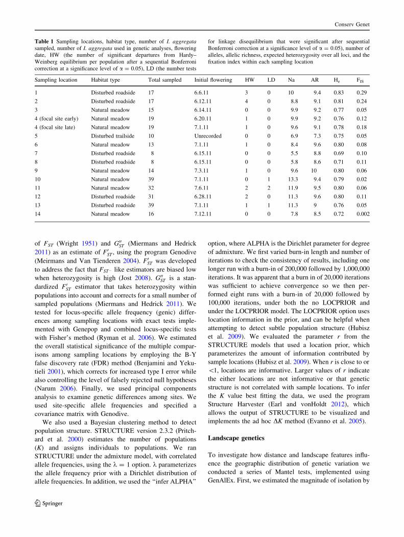
Table 1 Sampling locations, habitat type, number of I. aggregata

sampled, number of I. aggregata used in genetic analyses, flowering

date, HW (the number of significant departures from Hardy–

Weinberg equilibrium per population after a sequential Bonferroni

correction at a significance level of a = 0.05), LD (the number tests

for linkage disequilibrium that were significant after sequential

Bonferroni correction at a significance level of a = 0.05), number of

alleles, allelic richness, expected heterozygosity over all loci, and the

fixation index within each sampling location

Sampling location Habitat type Total sampled Initial flowering HW LD Na AR He FIS

1 Disturbed roadside 17 6.6.11 3 0 10 9.4 0.83 0.29

2 Disturbed roadside 17 6.12.11 4 0 8.8 9.1 0.81 0.24

3 Natural meadow 15 6.14.11 0 0 9.9 9.2 0.77 0.05

4 (focal site early) Natural meadow 19 6.20.11 1 0 9.9 9.2 0.76 0.12

4 (focal site late) Natural meadow 19 7.1.11 1 0 9.6 9.1 0.78 0.18

5 Disturbed trailside 10 Unrecorded 0 0 6.9 7.3 0.75 0.05

6 Natural meadow 13 7.1.11 1 0 8.4 9.6 0.80 0.08

7 Disturbed roadside 8 6.15.11 0 0 5.5 8.8 0.69 0.10

8 Disturbed roadside 8 6.15.11 0 0 5.8 8.6 0.71 0.11

9 Natural meadow 14 7.3.11 1 0 9.6 10 0.80 0.06

10 Natural meadow 39 7.1.11 0 1 13.3 9.4 0.79 0.02

11 Natural meadow 32 7.6.11 2 2 11.9 9.5 0.80 0.06

12 Disturbed roadside 31 6.28.11 2 0 11.3 9.6 0.80 0.11

13 Disturbed roadside 39 7.1.11 1 1 11.3 9 0.76 0.05

14 Natural meadow 16 7.12.11 0 0 7.8 8.5 0.72 0.002

Conserv Genet

123

distance by testing the correlation between geographic

distance and FST and F0ST . Second, after using STRUC-

TURE (described above) to assign individuals to genetic

groups, we qualitatively matched the resulting boundaries

among groups to physical aspects of the landscape. Third,

we investigated the extent to which elevation is associated

with genetic differentiation. We tested the extent to which

(1) the difference in the elevation of pairs of sites; and (2)

the cumulative elevation change among pairs of sites was

associated with genetic differentiation. We calculated the

cumulative elevation change between each pair of sam-

pling locations using the path tool available in Google

Earth version 7.0.

Relationship between flowering time and genetic

structure

We tested the extent to which genetic differentiation is

associated with flowering time in two ways. First, within

our focal site we marked I. aggregata plants before they

had flowered. We then conducted observations every other

day beginning on June 20, and recorded for each plant the

day that flowering began. Because flowering time was

somewhat episodic on this site (see Online Resource 8), we

subsequently divided plants into groups based on when

they first had an open flower, and designated two groups of

19 plants, an ‘‘early’’ and ‘‘late’’ group, between which

there was at least a 1 week difference in date of first

flowering. These two groups were intermixed geographi-

cally over the focal meadow, and there was overlap in the

flowering time of these groups, such that the plants in the

first flowering group were still flowering when the plants in

the second flowering group began flowering. We calculated

FST and F0ST between the two flowering groups.

Second, for each site, we sampled leaf tissue from plants

on the day that they first flowered. To ensure we accurately

recorded the date of first flowering we visited sites peri-

odically until we saw the consistent morphological changes

that I. aggregata undergoes before flowering; unopened

buds elongate and usually open the following day (Free-

man et al. 2003). We did this for 13 of the 14 sites.

However, one site was already in full flower when we

sampled it, and had no plants with unopened buds, so this

site was excluded from analyses that included flowering

time (Site 5; see ‘‘Results’’ section). After pinpointing the

date of first flowering for a site, we sampled only from

plants that had elongated buds, and sampled within 3 days

of the date of first flowering. We created a distance matrix

that contained the number of days apart that each pair of

sites had their first flowers, hereafter ‘phenological dis-

tance’. We then conducted a Mantel test to test the corre-

lation between genetic distances FST and F0ST , and

phenological distance. We conducted partial Mantel tests

implemented using the R statistical language (R develop-

ment core team 2008), and using the Vegan package

(Oksanen et al. 2011) to control for geographic distance

while testing for the correlation of genetic distances and

phenological distance. We also determined the correlation

between flowering date and elevation, and conducted par-

tial Mantel tests to test the correlation of flowering time

and genetic distance while controlling for elevation.

Mantel tests are one of the most common methods for

assessing the significance of the correlation between

matrices and have been widely applied in landscape genetic

analyses. However, there has been recent controversy over

their use due to low power and high Type I error rates

(Raufaste and Rousset 2001; Legendre and Fortin 2010;

Miermans 2015). Therefore, we also used a multiple

regression approach with a randomized permutation pro-

cedure (MMRR) that accounted for the non-independence

of variables, as described in Wang (2013). This procedure

may be preferable to Mantel tests because of more appro-

priate Type I error rates, and because it ranks variables in

terms of their relative effects on genetic distance (Wang

2013). We used MMRR implemented in R using the

function from Wang (2013), with 10,000 permutations, to

determine the independent contribution of geographic and

phenological distance to variation in genetic distances FST

and F0ST . We also incorporated the measure of elevational

distance among sites that had the highest Mantel correla-

tion with genetic distance (difference in elevation among

sites; see ‘‘Results’’ section) into the model used to predict

genetic distance.

Results

Genetic variation within populations

Mean number of alleles ranged from 5.5 to 13.3

(mean = 9.3, SD = 2.2) expected heterozygosity ranged

from 0.69 to 0.83 (mean = 0.77, SD = 0.02), and allelic

richness ranged from 7.3 to 10 (mean = 9.1, SD = 0.06;

Table 1). Prior to correction for multiple tests, 35 (29 %)

of all tests for departure from HW expectations were sig-

nificant (P = 0.05). After correction for multiple tests

using a Bonferroni procedure, 16 (13 %) of all tests were

significant (Table 1; Online Resource 1). Deviations from

HW expectations corresponded to a deficit of heterozy-

gotes within some sites; mean FIS ranged from 0.002 to

0.29 (Table 1). Some loci tended to deviate from HW

proportions more than others but a stronger pattern con-

sisted of multiple loci deviating from HW proportions

within certain populations (Online Resource 1). Prior to

Conserv Genet

123

correcting for multiple tests for linkage disequilibrium, 17

(6 %) were significant before and three (1 %) were sig-

nificant after a sequential Bonferroni correction. FIS was

significantly higher (t test, P = 0.006), expected

heterozygosity was significantly lower (t test, P = 0.04),

and allelic richness was marginally significantly lower

(t test, P = 0.078) among disturbed sites along trail or

roadsides than among sites in which the I. aggregata

expanded beyond the area (circle of radius 50 m) in which

we sampled.

Genetic differentiation among populations

There was moderate genetic differentiation among some

pairs of sites. Pairwise FST values ranged from 0 to 0.13

(average 0.04) and pairwise F0ST values ranged from 0 to

0.53 (average 0.19; Table 2). All but three of the 91 genic

tests of allele frequency differences among pairs of popu-

lations were significant before correcting for type I error.

After correcting for type I error, 82 (90 %) of the genic

tests were significant. The STRUCTURE results revealed

that there were two or three distinct genetic groups (K = 2

or 3), when we used sampling location as a prior, but

without the location prior, K = 1 had the strongest support

(Online Resource 2–4). When we used the LOCPRIOR

model, values of the r parameter were\1, which is con-

sistent with location information being informative in

delineating groups. For K = 3, the first cluster (red; Fig. 1)

contained sites that were located in the main drainage that

runs from Gunnison to Crested Butte. The second cluster

(green; Fig. 1) contained sites that were more peripheral to

this core drainage. The third cluster (blue; Fig. 1)

contained primarily one site (site 13) in the main drainage

that was completely surrounded by trees. For K = 2,

results were similar except that site 13 grouped with the

peripheral sites (Online Resource 4).

It is possible that drift caused allele frequencies to

converge in the peripheral sites and was responsible for

these STRUCTURE results. However, there was little

evidence that enhanced drift drove this pattern. Allelic

Richness and the proportion of the genome assigned to the

second genetic group (q value for K = 3 with LOCPRIOR)

were not correlated (r = 0.09, P = 0.41). There was some

evidence for clustering of peripheral sites with greater FIS

values, and therefore possibly with greater inbreeding

levels. There was no correlation between q values and the

number of significant departures from Hardy–Weinberg

equilibrium per population after a sequential Bonferroni

correction at a significance level of a = 0.05 (r = 0.2,

P = 0.52). Mean FIS and q values were not correlated

(r = 0.26, P = 0.37; Online Resource 5), however, with a

peripheral site that had unusually low FIS removed (site 14;

Online Resource 6), FIS and q values were significantly

correlated (r = 0.62, P = 0.02). In particular, two sites

outside of the core drainage appear to be driving the pattern

(sites 1 & 2; Table 1).

Additional evidence supports the STRUCTURE clus-

ters. First, the STRUCTURE results were mirrored by the

results of a principal component analysis (Online Resource

7). Second, a significant positive correlation between

pairwise F0ST values and difference in the average propor-

tion of the genome (q value) of individuals within sites that

was assigned to the first STRUCTURE genetic group

(Mantel test Rxy = 0.55, P = 0.001) demonstrates a close

Table 2 Genetic differentiation among all pairs of sites, with FST values above diagonal and F0ST values below diagonal

1 2 3 4 5 6 7 8 9 10 11 12 13 14

1 – 0.03 0.05 0.04 0.05 0.03 0.06 0.06 0.04 0.05 0.03 0.04 0.05 0.05

2 0.21 – 0.02 0.05 0.06 0.03 0.05 0.03 0.02 0.03 0.04 0.02 0.06 0.07

3 0.31 0.13 – 0.02 0.02 0.03 0.03 0.01 0.00 0.00 0.02 0.00 0.03 0.05

4 0.24 0.24 0.10 – 0.03 0.04 0.03 0.02 0.01 0.02 0.01 0.02 0.03 0.07

5 0.29 0.33 0.10 0.15 – 0.04 0.04 0.05 0.01 0.02 0.03 0.02 0.05 0.07

6 0.24 0.17 0.17 0.20 0.25 – 0.07 0.06 0.02 0.04 0.03 0.04 0.06 0.05

7 0.33 0.28 0.15 0.11 0.19 0.33 – 0.05 0.02 0.03 0.05 0.04 0.06 0.13

8 0.37 0.18 0.04 0.10 0.24 0.29 0.20 – 0.02 0.02 0.04 0.03 0.05 0.08

9 0.24 0.11 0.00 0.03 0.08 0.15 0.10 0.08 – 0.00 0.02 0.01 0.02 0.07

10 0.29 0.16 0.00 0.09 0.11 0.21 0.14 0.10 0.00 – 0.02 0.01 0.03 0.06

11 0.16 0.25 0.12 0.07 0.16 0.18 0.24 0.17 0.11 0.12 – 0.02 0.04 0.03

12 0.24 0.14 0.02 0.11 0.12 0.24 0.18 0.13 0.05 0.06 0.11 – 0.03 0.05

13 0.31 0.30 0.13 0.15 0.23 0.30 0.25 0.20 0.11 0.12 0.18 0.16 – 0.07

14 0.28 0.33 0.24 0.29 0.31 0.23 0.53 0.33 0.32 0.28 0.16 0.24 0.29 –

Bold values indicate pairwise comparisons that were not significant based on genic tests for population differentiation before or after Bonferroni

correction, and italicized cells indicate pairwise comparisons that were not significant after Bonferroni correction

Conserv Genet

123

correspondence between F0ST and the STRUCTURE

results.

There was no evidence of isolation by distance over the

area sampled. Geographic distance and FST (Mantel test

Rxy = 0.01, P = 0.44) or F0ST (Mantel test Rxy = 0.08,

P = 0.36) were not significantly correlated. We also found

no evidence that elevation was associated with genetic

structure of I. aggregata. There was no significant corre-

lation of FST or F0ST and cumulative difference in elevation

among pairs of sites (Mantel test Rxy = -0.05, P = 0.48

for FST; Rxy = 0.02; P = 0.43 for F0ST ; range of cumulative

elevation change distances was 866–20,072 m) or of dif-

ference in elevation among pairs of sites (Mantel test

Rxy = 0.19; P = 0.10 for FST; Rxy = 0.07; P = 0.33 for

F0ST ). Three sites comprised the three pairs of sites that

were the most genetically similar but they were not geo-

graphically adjacent. These were separated by 28, 24, and

9.4 km, and had cumulative elevation changes of 2252,

3341, and 2737 m, but were located along the one main

drainage in the geographic area sampled.

Association of flowering time and genetic structure

We found a strong association between flowering time and

genetic structure in I. aggregata. Within our focal meadow,

the plants we marked began to flower on June 20, and

individual plants began flowering into July (Online

Resource 8). There was moderate genetic differentiation

between plants in our ‘‘early’’ flowering group—those that

flowered on or before June 23, and plants in our ‘‘late’’

flowering group—those that flowered on or after June 30

(FST = 0.05; F0ST ¼ 0:23; genic test for population differ-

entiation combined P value \0.001). Across all popula-

tions, sites at higher altitudes tended to flower later in the

summer (correlation between flowering time and eleva-

tion = 0.66, P = 0.01). Notably, one of the sampling

locations that STRUCTURE identified as being genetically

distinct (Site 14) was the last to begin flowering, which

occurred 36 days after a flower opened at the earliest-

flowering sampling location. Another genetically distinct

location also flowered late with respect to the other sam-

pling locations; Site 13 was the 11th out of 14 sites to begin

flowering.

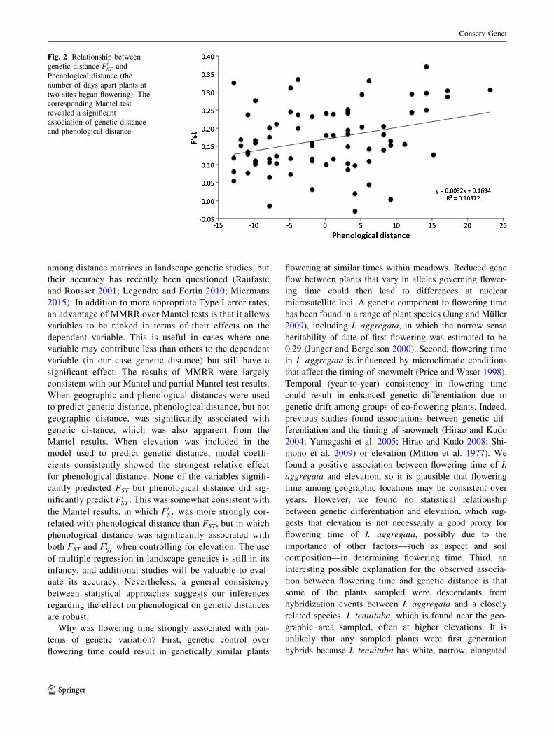
Results from Mantel tests and MMRR analysis indicated

that flowering time was associated with genetic structure.

There was a significant correlation between phenological

distance (defined as difference in flowering time) and FST

(Mantel test Rxy = 0.29, P = 0.015) and F0ST (Mantel test

Rxy = 0.32, P = 0.009; Fig. 2). When controlling for

geographic distance there was a significant correlation

between phenological distance and FST (Partial Mantel test

Rxy = 0.31, P = 0.025), and F0ST (Partial Mantel test

Rxy = 0.32, P = 0.013). When controlling for elevation

there was a significant correlation between phenological

distance and FST (Partial Mantel test Rxy = 0.24,

P = 0.047), and F0ST (Partial Mantel test Rxy = 0.30,

P = 0.018). From the MMRR used to predict genetic

distance FST from geographic and phenological distances,

phenological distance had a higher regression coefficient

than geographic distance, and only phenological distance

significantly predicted genetic distance (geographic dis-

tance: b = -0.03, P = 0.90; phenological distance:

b = 0.29, P = 0.03). The pattern was the same for F0ST

(geographic distance: b = 0.03, P = 0.89; phenological

distance: b = 0.30, P = 0.02). When difference in eleva-

tion among sites was included as an independent variable

in addition to geographic and phenological distances, no

independent variable significantly predicted FST (geo-

graphic distance: b = -0.02, P = 0.92; elevation:

b = 0.14, P = 0.38; phenological distance: b = 0.25,

P = 0.11). However, with elevation included as an inde-

pendent variable phenological distance did significantly

predict F0ST (geographic distance: b = -0.03, P = 0.89;

elevation: b = 0.01, P = 0.96; phenological distance:

b = 0.30, P = 0.05).

Discussion

We found significant genetic structuring and an association

of flowering time and genetic differentiation in the mono-

carpic montane perennial I. aggregata. Many studies that

attempt to explain patterns of genetic structure incorporate

distance or landscape factors (Manel and Holderegger

2013). Adding phenological data may generally help better

explain the geographic distribution of genetic variation

(Hendry and Day 2005). This is particularly important in

systems in which interacting species may influence levels

of gene flow in populations of their partner species. For

plants, gene flow occurs via pollen transfer among co-

flowering plants, and phenological differences among

plants can contribute to genetic distances among them

(Hirao and Kudo 2004; Yamagashi et al. 2005; Hirao and

Kudo 2008). In this study, we incorporated flowering time

into statistical frameworks used in landscape genetics

analyses, and we found that flowering time, but not dis-

tance or elevation, was significantly correlated with genetic

structure of I. aggregata, both within a meadow over 80 m

and over a large geographic area within which the farthest

two sampling locations were 130 km.

We examined the association between phenological

distance and genetic distance using both Mantel tests and

the MMRR method described in Wang (2013). Mantel tests

have been the standard way to test for an association

Conserv Genet

123

among distance matrices in landscape genetic studies, but

their accuracy has recently been questioned (Raufaste

and Rousset 2001; Legendre and Fortin 2010; Miermans

2015). In addition to more appropriate Type I error rates,

an advantage of MMRR over Mantel tests is that it allows

variables to be ranked in terms of their effects on the

dependent variable. This is useful in cases where one

variable may contribute less than others to the dependent

variable (in our case genetic distance) but still have a

significant effect. The results of MMRR were largely

consistent with our Mantel and partial Mantel test results.

When geographic and phenological distances were used

to predict genetic distance, phenological distance, but not

geographic distance, was significantly associated with

genetic distance, which was also apparent from the

Mantel results. When elevation was included in the

model used to predict genetic distance, model coeffi-

cients consistently showed the strongest relative effect

for phenological distance. None of the variables signifi-

cantly predicted FST but phenological distance did sig-

nificantly predict F0ST . This was somewhat consistent with

the Mantel results, in which F0ST was more strongly cor-

related with phenological distance than FST, but in which

phenological distance was significantly associated with

both FST and F0ST when controlling for elevation. The use

of multiple regression in landscape genetics is still in its

infancy, and additional studies will be valuable to eval-

uate its accuracy. Nevertheless, a general consistency

between statistical approaches suggests our inferences

regarding the effect on phenological on genetic distances

are robust.

Why was flowering time strongly associated with pat-

terns of genetic variation? First, genetic control over

flowering time could result in genetically similar plants

flowering at similar times within meadows. Reduced gene

flow between plants that vary in alleles governing flower-

ing time could then lead to differences at nuclear

microsatellite loci. A genetic component to flowering time

has been found in a range of plant species (Jung and Muller

2009), including I. aggregata, in which the narrow sense

heritability of date of first flowering was estimated to be

0.29 (Junger and Bergelson 2000). Second, flowering time

in I. aggregata is influenced by microclimatic conditions

that affect the timing of snowmelt (Price and Waser 1998).

Temporal (year-to-year) consistency in flowering time

could result in enhanced genetic differentiation due to

genetic drift among groups of co-flowering plants. Indeed,

previous studies found associations between genetic dif-

ferentiation and the timing of snowmelt (Hirao and Kudo

2004; Yamagashi et al. 2005; Hirao and Kudo 2008; Shi-

mono et al. 2009) or elevation (Mitton et al. 1977). We

found a positive association between flowering time of I.

aggregata and elevation, so it is plausible that flowering

time among geographic locations may be consistent over

years. However, we found no statistical relationship

between genetic differentiation and elevation, which sug-

gests that elevation is not necessarily a good proxy for

flowering time of I. aggregata, possibly due to the

importance of other factors—such as aspect and soil

composition—in determining flowering time. Third, an

interesting possible explanation for the observed associa-

tion between flowering time and genetic distance is that

some of the plants sampled were descendants from

hybridization events between I. aggregata and a closely

related species, I. tenuituba, which is found near the geo-

graphic area sampled, often at higher elevations. It is

unlikely that any sampled plants were first generation

hybrids because I. tenuituba has white, narrow, elongated

Fig. 2 Relationship between

genetic distance F0ST and

Phenological distance (the

number of days apart plants at

two sites began flowering). The

corresponding Mantel test

revealed a significant

association of genetic distance

and phenological distance

Conserv Genet

123

corollas, hybrids have bright pink, slightly shorter corollas

(Melendez-Ackerman et al. 1997) and we sampled only in

areas in which all plants had bright red corollas. Never-

theless, this is an interesting possibility and would be worth

investigating if species-specific markers are developed.

It was surprising that even within a meadow, plants

that began flowering more than 1 week apart were sig-

nificantly genetically differentiated. This is consistent with

temporal isolation and early stages of reproductive isola-

tion. Temporal isolation within populations has been

observed with other species of plants (Antonovics 2006)

and animals (e.g. Pacific salmon; Kovach et al. 2013).

Temporal isolation of this type may be unlikely in Ipo-

mopsis aggregata because plants can sometimes produce

tens of flowers that open successively over time, and

within our focal meadow there was some overlap in

flowering time between early and later flowering plants

(S. Suni, personal observation). An alternative explanation

is that separate cohorts may flower at different times.

Campbell (1997) found that the age at which I. aggregata

plants flower ranges from 2 to 10 years, so it is possible

that the genetic differentiation observed could be due to

among-cohort genetic drift in cohorts that flower at

slightly different times during the summer. Additionally,

though early and later flowering plants were intermixed

geographically we cannot rule out the possibility that

flowering time differences were driven by microenviron-

mental differences that persist over time.

The observed structure among sites appears to be weak

but biologically meaningful. The fact that inference of

K[ 1 occurred only when we used a location prior with

STRUCTURE is consistent with weak divergence among

populations. However, low values of the r parameter sup-

ported inference of a correlation between geographic

location and genetic differentiation. Care must also be used

in interpreting our STRUCTURE results because evidence

for elevated inbreeding within populations of this species

violates an assumption of the model. Mild departures from

the model used to partition individuals into genetic groups

can lead to an overestimation of the number of clusters

with STRUCTURE (Falush et al. 2003). In particular, if

linkage disequilibrium among loci is due not to actual

population structure, but instead to inbreeding, K might be

overestimated. In our case, the third genetic group had only

one Hardy–Weinberg violation and one significant LD test,

suggesting that it is not inbreeding that resulted in it

seeming genetically distinct. For the remaining sites, there

was no significant correlation of number of departures from

Hardy–Weinberg equilibrium or FIS and the proportion of

the genome assigned to the second genetic group among

sites. However when the site with the lowest FIS was

removed from the analysis, FIS was significantly correlated

with the proportion of the genome assigned to the second

genetic group, suggesting that inbreeding could be partially

responsible for STRUCTURE’s delineations.

The results from STRUCTURE were supported by anal-

yses based on F-statistics and PCA. These results suggest

that gene flow occurs within the central drainage and that

genetic drift might be responsible for differentiation of the

sites that are more peripheral to this drainage. Gene flow

within the central drainage could occur via pollinator sharing

among co-flowering plants. Gene flow in I. aggregata is

thought to occur primarily by pollen transfer by broad-tailed

and rufous hummingbirds (Selasphorus platycercus and S.

rufus), but bumble bees such as Bombus appositus, solitary

bees, and butterflies also visit (Waser 1982). In years when

bumble bees are frequent visitors they are likely important

pollinators because they transfer on average three times as

much pollen and elicit about four times as much seed pro-

duction as hummingbirds (Mayfield et al. 2001). However, it

is unknown how far insects transfer pollen, or how fre-

quently insects visited the I. aggregata plants that were the

parents of those sampled in this study. Previous work using

dyes as pollen analogues showed that rufous hummingbirds

travel on average 0.8 m between plants when foraging

within a meadow (Waser 1982), and that more than 95 % of

transfer of an experimental pollen analog seemed to occur

within 5 m (Waser and Price 1983). However, both species

of hummingbirds presumably could transfer pollen longer

distances. Alternatively, seed dispersal could occur via

water transport. Previous work estimated that the root mean

square seed dispersal distance was 0.6 m (Waser and Price

1983), though it is conceivable that during heavy rains, seeds

may be washed down slopes. Evaluating the extent to which

seed dispersal contributes to gene flow in I. aggregatawould

require additional tests.

For the peripheral sites, allele frequencies at the rela-

tively few loci we examined might have drifted in the same

direction by chance. However, if genetic drift was

responsible for the observed pattern we may expect a

corresponding decrease in heterozygosity and allelic rich-

ness within the peripheral sites, but no such pattern was

found. Another possibility is that the breeding structure of

I. aggregata influenced the way in which individuals were

partitioned into genetic groups. Ipomopsis aggregata exist

as hardy rosettes for a number of years before bolting,

flowering, and senescence. If different sites were made up

largely of plants that germinated in different years, genetic

differences among cohorts could be at least partially

responsible for the modest allele frequency divergence we

observed. The observed higher mean FIS in peripheral sites

suggests that inbreeding is also at least partially responsible

for our STRUCTURE results. Even if the STRUCTURE

results were partially driven by inbreeding as a violation of

the underlying model, these results remain important from

a conservation perspective. Small peripheral sites with

Conserv Genet

123

elevated inbreeding levels could be suffering from

inbreeding depression and may have lower resilience.

Our results are consistent with those obtained from

previous population genetic studies of I. aggregata. We

found significant genetic differentiation among sites that

were as little as 2.6 km apart, and significant differentiation

within a site among plants with different flowering phe-

nology. Previous population genetic analyses using allo-

zymes revealed positive spatial autocorrelation of allele

frequencies over just 5 m (Campbell and Dooley 1992),

and significant structuring over 25 km (Wolf and Campbell

1995). Interestingly, Wolf and Campbell (1995) found that

genetic structure increased more from 250 m to 2.5 km

than it did from 2.5 to 25 km, which was likely the result of

family structure.

Our results also suggest that strong family structure

occurs within sites; we found high FIS values and

heterozygote deficits within some sites, which can occur

when there is breeding among close relatives (Wright

1922). This may seem surprising given the mating system

of I. aggregata, in which plants are self-incompatible and

may be expected to mate disassortatively with unrelated

individuals. However, It is not uncommon for self-incom-

patible plants to show a deficiency of heterozygotes (Levin

1978; Turner et al. 1982; Barluenga et al. 2011), and four

pieces of evidence suggest that a deficit of heterozygotes

may actually be expected in populations of I. aggregata.

First, the combination of limited seed dispersal and a

propensity of pollinators to move between neighboring

plants (Waser 1982) means that plants may often mate with

close relatives. Second, I. aggregata seems to suffer from

outbreeding depression over just 100 m (Waser and Price

1989), suggesting that to some extent matings between

individuals with more similar genotypes may be more

successful relative to those with less similar genotypes.

Third, many of the sites with higher FIS values were in

disturbed areas along trail or roadsides, and, thus may not

be part of large, stable populations. These possibly more

ephemeral populations seem to have relatively high

inbreeding rates, which is likely partially responsible for

the FIS observations. It is possible that higher inbreeding

rates lead to inbreeding depression (reduced fitness asso-

ciated with inbreeding) in small populations that occur in

suboptimal habitat. Evidence that inbreeding depression

occurs in small I. aggregata populations comes from a

study that found larger fitness gains in small relative to

large populations following pollen transfer (Heschel and

Paige 1995). Finally, a deficiency of heterozygotes relative

to Hardy–Weinberg expectations could result from sam-

pling individuals that belong to multiple randomly mating

cohorts. The I. aggregata that we sampled could have

germinated in different years, which could also contribute

to the observed deficiency of heterozygotes.

Overall, our results suggest that patterns of genetic

diversity and differentiation in I. aggregata may be par-

tially explained by inbreeding within sites and phenologi-

cal differences within and among sites. Sites in disturbed,

human dominated areas along trail or roadsides had lower

genetic diversity and higher FIS than sites in more natural

meadows, suggesting a possible positive association

between anthropogenic disturbance and localized popula-

tion extinctions and a negative association between

anthropogenic disturbance and adaptive potential for I.

aggregata. However, the markers used to assess these

patterns were neutrally evolving microsatellites, so it

would be useful to investigate the extent to which genome-

wide patterns of genetic diversity and local adaptation

differ among plants in disturbed versus more natural areas.

In terms of structure among sites, cohesion we observed

among sites in the main drainage may have been the result

of pollinator movement, and pollinators may have been

cueing in on landscape factors not included in our analysis,

such as lack of tree cover, when travelling. Alternatively,

rain-mediated seed dispersal down drainages may partly

contribute to gene flow, although seed dispersal may be

expected to decrease the association of flowering time and

genetic structure. The strong association between flowering

time and genetic structure that we observed suggests that

pollinator-mediated pollen movement among co flowering

plants is an important mechanism by which gene flow

occurs in I. aggregata. These results have important

implications for understanding how the geographic distri-

bution of genetic variation might change under future cli-

mate change scenarios that likely include phenological

changes such as flowering time.

Acknowledgments We thank Matt Kaplan and the staff of the

Genomics Core Facility at the University of Arizona for help with

microsatellite genotyping; the Rocky Mountain Biological Laboratory

in Gothic, CO, for support and use of facilities and equipment, and

Judith Bronstein and Nickolas Waser for help and guidance during

fieldwork. This work was funded in part also by NIH Grant 5 K12

GM000708, which was awarded to the Center for Insect Science at

the University of Arizona, and by support from the University of

Massachusetts Amherst to S. Suni while she was the Darwin Fellow.

References

Allendorf FW, Luikart G (2007) Genetics and the conservation of

populations. Blackwell Publishing, Hoboken

Antonovics J (2006) Evolution in closely adjacent plant populations

X: long-term persistence of prereproductive isolation at a mine

boundary. Heredity 97:33–37

Barluenga M, Austerliz F, Elzinga JA, Teixeira S, Goudet J,

Bernasconi G (2011) Fine-scale spatial genetic structure and

gene dispersal in Silene latifolia. Heredity 106:13–24

Benjamini Y, Yukutieli D (2001) The control of the false discovery

rate in multiple testing under dependency. Ann Stat

29:1165–1188

Conserv Genet

123

Campbell DR (1997) Genetic and environmental variation in life

history traits of a monocarpic perennial: a decade-long field

experiment. Evolution 51:373–382

Campbell DR, Dooley JL (1992) The spatial scale of genetic

differentiation in a hummingbird-pollinated plant: comparison

with models of isolation by distance. Am Nat 139:735–748

Colautti RI, Barrett SCH (2013) Rapid adaptation to climate

facilitates range expansion of an invasive plant. Science

342:364–366

Cortes AJ, Waeber S, Lexer C, Sedlacek J, Wheeler JA, van Kleunen

M et al (2014) Small-scale patterns in snowmelt timing affect

gene flow and the distribution of genetic diversity in the alpine

dwarf shrub Salix herbacea. Heredity. doi:10.1038/hdy.2014.19

Dunne JA, Harte J, Taylor KJ (2003) Subalpine meadow flowering

phenology responses to climate change: integrating experimental

and gradient methods. Ecol Monogr 73:69–86

Earl DA, vonHoldt BM (2012) STRUCTURE HARVESTER: a

website and program for visualizing STRUCTURE output and

implementing the Evanno method. Cons Gen Res 4:259–361

Ennos RA (1994) Estimating the relative rates of pollen and seed

migration among plant populations. Nature 72:250–259

Evanno G, Regnaut S, Goudet J (2005) Detecting the number of

clusters of individuals using the software STRUCTURE: a

simulation study. Mol Ecol 14:2611–2620

Falush D, Stephens M, Pritchard J (2003) Inference of population

structure using multilocus genotypic data: linked loci and

correlated allele frequencies. Genetics 164:1567–1587

Fenster CB (1991) Gene flow in Chamaecrista fasciculate (Legumi-

nosae) I. Gene dispersal. Evolution 45:398–409

Fox GA (2003) Assortative mating and plant phenology: evolutionary

and practical consequences. Evolut Ecol Res 5:1–18

FrankhamR (2010)Challenges and opportunities of genetic approaches

to biological conservation. Biol Conserv 143:1919–1927

Freeman RS, Brody AK, Neefus CD (2003) Flowering phenology and

compensation for herbivory in Ipomopsis aggregata. Oecologia

136:394–401

Geber MA, Griffen LR (2003) Inheritance and natural selection on

functional traits. Int J Plant Sci 164:S21–S42

Gerber J-D, Baltisberger M, Leuchtmann A (2004) Effects of a

snowmelt gradient on the population structure of Ranunculus

alpestris. Bot Helv 114:67–78

Gilpin M, Hanski I (1991) Metapopulation dynamics: empirical and

theoretical investigations. Academic Press, London

Hall MC, Willis JH (2006) Divergent selection on flowering time

contributes to local adaptation in Mimulus guttatus populations.

Evolution 60:2466–2477

Hendry AP, Day T (2005) Population structure attributable to

reproductive time: isolation by time and adaptation to time.

Mol Ecol 14:901–916

Heschel MS, Paige KN (1995) Inbreeding depression, environmental

stress, and population size variation in Scarlet Gilia (Ipomopsis

aggregata). Conserv Biol 9:126–133

Hirao AS, Kudo G (2004) Landscape genetics of alpine-snowbed

plants: comparisons along geographic and snowmelt gradients.

Heredity 93:290–298

Hirao AS, Kudo G (2008) The effect of segregation of flowering time

on fine-scale spatial genetic structure in an alpine-snowbed herb

Primula cuneifolia. Heredity 100:424–430

Holderegger R, Wagner HH (2008) Landscape genetics. Bioscience

58:199–207

Hubisz MJ, Falush D, Stephens M, Pritchard JK (2009) Inferring

weak population structure with the assistance of sample group

information. Mol Ecol Res 9:1322–1332

Inouye DW, McGuire AD (1991) Effects of snowpack on timing and

abundance of flowering in Delphinium nelsonii (Ranunculaceae):

implications for climate change. Am J Bot 78:997–1001

Jay F, Manel S, Alvarez N, Durand EY, Thuiller W, Holderegger R,

Taberlet P, Francois O (2012) Forecasting changes in population

genetic structure of alpine plants in response to global warming.

Mol Ecol 21:2354–2368

Jost L (2008) GST and its relatives do not measure differentiation.

Mol Ecol 17:4015–4026

Jung C, Muller AE (2009) Flowering time control and applications in

plant breeding. Trends Plant Sci 14:563–567

Junger T, Bergelson Y (2000) The evolution of compensation to

herbivory in Scarlet Gilia, Ipomopsis aggregata: herbivore-

imposed natural selection and the quantitative genetics of

tolerance. Evolution 54:764–777

Keller SR, Levsen N, Ingvarsson PK, Olson MS, Tiffin P (2011)

Local selection across a latitudinal gradient shapes nucleotide

diversity in balsam poplar, Populus balsamifera L. Genetics

188:941–952

Kittelson PM, Maron JL (2001) Fine-scale genetically based differ-

entiation of life history traits in the perennial shrub Lupinus

arboreus. Evolution 55:2429–2438Korves TM, Schmid KJ, Caicedo AL, Mays C, Stinchcombe JR,

Purugganan MD, Schmitt J (2007) Fitness effects associated with

the major flowering time gene FRIGIDA in Arabidopsis thaliana

in the field. Am Nat 169:E141–E157

Kovach RP, Gharrett J, Tallmon DA (2013) Temporal patterns of

genetic variation in a salmon population undergoing rapid

change in migration timing. Evol App 6:795–807

Lambert AM, Miller-Rushing AJ, Inouye D (2010) Changes in

snowmelt date and summer precipitation affect the flowering

phenology of Erythronium grandiflorum (glacier lily; Liliaceae).

Am J Bot 97:1431–1437

Legendre P, Fortin M (2010) Comparison of the Mantel test and

alternative approaches for detecting complex multivariate rela-

tionships in the spatial analysis of genetic data. Mol Ecol Res

10:831–844

Levin D, Kerster HW (1974) Gene flow in seed plants. Evol Biol

7:139–220

Levin D (1978) Genetic variation in annual Phlox: self-compatible

versus self-incompatible species. Evolution 32:245–263

Manel S, Holderegger R (2013) Ten years of landscape genetics.

Trends Ecol Evol 28:613–621

Manel S, Schwartz MK, Luikart G, Taberlet P (2003) Landscape

genetics: combining landscape ecology and population genetics.

Trends Ecol Evol 18:189–197

Mayfield MM, Waser NM, Price MV (2001) Exploring the ‘most

effective pollinator principle’ with complex flowers: bumblebees

and Ipomopsis aggregata. Ann Bot-Lond 88:591–596

Meirmans PG, Van Tienderen PH (2004) GENOTYPE and

GENODIVE: two programs for the analysis of genetic diversity

of asexual organisms. Mol Ecol Notes 4:792–794

Melendez-Ackerman E, Campbell DR, Waser NM (1997) Humming-

bird behavior and mechanisms of flower color in Ipomopsis.

Ecology 78:2532–2541

Miermans PG (2015) Seven common mistakes in population genetics

and how to avoid them. Mol Ecol 13:3223–3231

Miermans PG, Hedrick PW (2011) Assessing population structure:

FST and related measures. Mol Ecol Res 11:5–18

Mitton JB, Linhart YB, Hamrick JL, Beckman J (1977) Population

differentiation and mating systems in ponderosa pine in the

Colorado Front range. Theor App Genet 51:5–14

Narum SR (2006) Beyond Bonferroni: less conservative analyses for

conservation genetics. Con Gen 7:783–787

Nei M (1987) Molecular evolutionary genetics. Columbia University

Press, New York

Oksanen JF, Guillaume B, Kindt R, Legrende R, et al (2011) Vegan:

community ecology package. R package version 1.17-10. http://

cran.r-project.org/web/packages/vegan/

Conserv Genet

123

Parmesan C, Yohe G (2003) A globally coherent fingerprint of

climate change impacts across natural systems. Nature

421:37–42

Peakall ROD, Smouse PE (2006) genalex 6: genetic analysis in Excel.

Population genetic software for teaching and research. Mol Ecol

Notes 6:228–295

Price M, Waser N (1998) Effects of experimental warming on plant

reproductive phenology in a subalpine meadow. Ecology

79:1261–1271

Pritchard JM, Stephens M, Donnelly P (2000) Inference of population

structure using multilocus genotype data. Genetics 155:945–959

R Core Team (2008) A language and environment for statistical

computing. R Foundation for Statistical Computing, Vienna,

Austria. http://www.R-project.org/

Raufaste N, Rousset F (2001) Are partial Mantel tests adequate?

Evolution 55:1703–1705

Rousset F (2008) GENEPOP’007: a complete re-implementation of

the GENEPOP software for Windows and Linux. Mol Ecol Res

8:103–106

Ryman N, Palm S, Andre C, Carvalho GR, Dahlgren TG, Jorde PE,

Laikre L, Larsson LC, Palme A, Ruzzante DE (2006) Power for

detecting genetic divergence: differences between statistical

methods and marker loci. Mol Ecol 15:2031–2045

Saccheri I, Kuussaari M, Kankare M, Vikman P, Fortelius W, Hanski

I (1998) Inbreeding and extinction in a butterfly metapopulation.

Nature 392:491–494

Shimono Y, Watanabe M, Hirao AS, Wada N, Gaku K (2009)

Morphological and genetic variations of Potentilla matsumurae

(Rosacae) between fellfield and snowbed populations. Am J Bot

96:728–737

Shindler et al (2010) Population diversity and the portfolio effect in

an exploited species. Nature 465:609–613

Soule ME (1987) Viable populations for conservation. Cambridge

University Press, Cambridge

Stanton ML, Galen C, Shore JS (1997) Population structure along a

steep environmental gradient: consequences of flowering time

and habitat variation in the snow buttercup, Ranunculus adoneus.

Evolution 51:79–94

Stanton ML, Roy BA, Thiede DA (2000) Evolution in stressful

environments. I. Phenotypic variability, phenotypic selection,

and response to selection in five distinct environmental stresses.

Evolution 54:93–111

Stinchcomb JR, Weinig C, Ungerer M, Olsen KM, Mays C,

Halldorsdottir SS, Purugganan MD, Schmitt J (2004) A latitu-

dinal cline in flowering time in Arabidopsis thaliana modulated

by the flowering time gene FRIGIDA. Proc Nat Acad Sci

101:4712–4717

Storfer A, Murphy MA, Evans JS, Goldberg CS, Robinson S, Spear

SF, Dezzani R, Delmelle E, Vierling L, Waits L (2007) Putting

the ‘‘landscape’’ in landscape genetics. Heredity 98:128–142

Turner ME, Stephens JC, Anderson WW (1982) Homozygosity and

patch structure in plant populations as a result of nearest-

neighbor pollination. Proc Nat Acad Sci 79:203–207

Wang JI (2013) Examining the full effects of landscape heterogeneity

on spatial genetic variation: a multiple matrix regression

approach for quantifying geographic and ecological isolation.

Evolution 67:3403–3411

Waser NM (1982) A comparison of distances flown by different

visitors to flowers of the same species. Oecologia 55:251–257

Waser NM, Price MV (1983) Optimal and actual outcrossing, and the

nature of plant-pollinator interaction. In: Jones CE, Little RJ

(eds) Handbook of experimental pollination biology. Van

Nostrand Reinhold, New York, pp 341–359

Waser NM, Price MV (1989) Optimal outcrossing in Ipomopsis

aggregata: seed set and offspring fitness. Evolution

43:1097–1109

Weis AE, Kossler TM (2004) Genetic variation in flowering time

induces phenological assortative mating: quantative genetic

methods applied to Brassica rapa. Am J Bot 91:825–836

Wolf PG, Campbell DR (1995) Hierarchical analysis of allozymic and

morphometric variation in a montane herb, Ipomopsis aggregata

(Polemoniaceae). J Heredity 86:386–394

Wright S (1922) Coefficients of inbreeding and relationship. Am Nat

56:330–338

Wright S (1943) Isolation by distance. Genetics 28:114–138

Wright S (1951) The genetical structure of natural populations. Ann

Eug 15:323–354

Wu C (2006) Characterization of microsatellite loci in Ipomopsis

(Polemoniaceae) wildflowers. Mol Ecol Res 6:921–923

Yamagashi H, Allison TD, Ohara M (2005) Effect of snowmelt

timing on the genetic structure of an Erythronium grandiflorum

population in an alpine environment. Ecol Res 20:199–204

Conserv Genet

123