Genetic Dominance in Extended Pedigrees: Boulder, March 2008 Irene Rebollo Biological Psychology...

Genetic Dominance in Extended Pedigrees:Boulder, March 2008

Irene Rebollo

Biological Psychology Department, Vrije Universiteit

Netherlands Twin Register

Dominance and Personality

•Nonadditive genetic variance

Individual differences due to effects of alleles (dominance) or loci (epistasis) that interact with other alleles or loci.

•Prevalent in Personality:

Keller, M. C., Coventry, W. L., Heath, A. C., & Martin, N. G. (2005). Widespread evidence for non-additive genetic variation in Cloninger's and Eysenck's personality dimensions using a twin plus sibling design. Behavior Genetics, 35, 707-721.

Penke, L., Denissen, J. J., & Miller, G. F. (2007). The evolutionary genetics of personality. European Journal of Personality, 21, 549-587.

Genetic relatedness of DZ twins

A1 A2

A3 A3A1 A3A2

A4 A4A1 A4A2

A3A1 A3A2 A4A1 A4A2

A3A1 2 1 1 0

A3A2 1 2 0 1

A4A1 1 0 2 1

A4A2 0 1 1 2

Possible Siblings

Average number of alleles shared:

116

42

16

81

16

40

25% non-additive genetic effects

50% additive genetic effects

Mot

he

rFather

ADE with Classic Twin Design: Identification

If rDZ < ½ rMZ

V = 1 = a2+d2+e2

rMZ = a2 + d2

rDZ = ½ a2 + ¼ d2

a2 = 4rDZ - rMZ

d2 = 2rMZ - 4rDZ

e2 = 1-rMZ

If rDZ > ½ rMZ

V = 1 = h2+c2+e2

rMZ = h2 + c2

rDZ = ½ h2 + c2

h2 = 2(rMZ - rDZ)

c2 = rMZ – h2

e2 = 1-rMZ

A D E

Twin 1

E D A

Twin 2

MZ: 1 / DZ: 0.25

MZ: 1 / DZ: 0.5

1 1 1 1 1 1

ad

e ad

e

MZ twin covariance matrix

TW1 TW2

TW1

TW2

DZ twin covariance matrix

TW1 TW2

TW1

TW2

a2+d2

a2+d2

0.5a2+0.25d2

a2+d2+e2

a2+d2+e2

a2+d2+e2

a2+d2+e2

0.5a2+0.25d2

ADE with Classic Twin Design

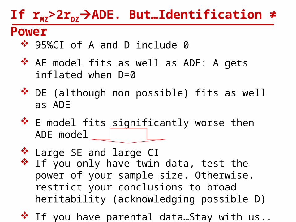
If rMZ>2rDZADE. But…Identification ≠ Power

95%CI of A and D include 0

AE model fits as well as ADE: A gets inflated when D=0

DE (although non possible) fits as well as ADE

E model fits significantly worse then ADE model

Large SE and large CI

If you only have twin data, test the power of your sample size. Otherwise, restrict your conclusions to broad heritability (acknowledging possible D)

If you have parental data…Stay with us..

Power

Definition: The expected proportion of samples in which we decide correctly against the null hypothesis

Depends on:

Effect considered (e.g. A or D)

Size of the effect in the population

Probability level adopted

Sample size

Composition of the sample: which kinds of relatives and in which proportion?

Level of measurement (categorical, ordinal, continuous)(p.191;Neale & Cardon, 1992)

Power of Classic Twin Design

Mx Script powerADEtwins.mx! Step 1: Simulate the data for power calculation of ACE model! 30% additive genetic (.5477²=.3)! 20% common environment (.4472²=.2)! 50% random environment (.7071²=.5)

#NGroups 3G1: model parameters Calculation Begin Matrices;

X Lower 1 1 Fixed ! genetic structureW Lower 1 1 Fixed ! non-additive genetic structure

Z Lower 1 1 Fixed ! specific environmental structureH Full 1 1Q Full 1 1

End Matrices; 1

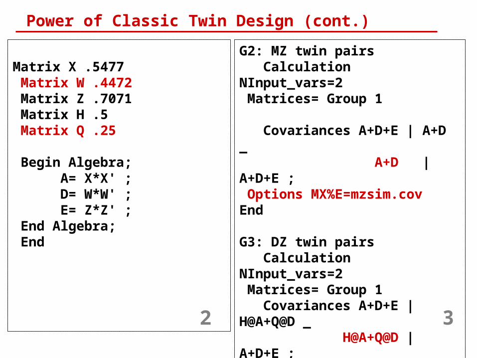
Power of Classic Twin Design (cont.)

Matrix X .5477 Matrix W .4472 Matrix Z .7071 Matrix H .5 Matrix Q .25 Begin Algebra;

A= X*X' ;D= W*W' ;E= Z*Z' ;

End Algebra; End

G2: MZ twin pairs Calculation NInput_vars=2 Matrices= Group 1

Covariances A+D+E | A+D _ A+D | A+D+E ;

Options MX%E=mzsim.covEnd

G3: DZ twin pairs Calculation NInput_vars=2 Matrices= Group 1 Covariances A+D+E | H@A+Q@D _

H@A+Q@D | A+D+E ;Options MX%E=dzsim.covEnd

2 3


!________________________________! Step 2: Fit the wrong model to the simulated data


X Lower 1 1 Free W Lower 1 1 FixedZ Lower 1 1 FreeH Full 1 1Q Full 1 1

End Matrices;

Matrix H .5 Matrix Q .25

Begin Algebra;A= X*X' ;D= W*W' ;E= Z*Z' ;

End Algebra; End

G2: MZ twin pairs Data NInput_vars=2 NObservations=1000 CMatrix Full File=mzsim.cov Matrices= Group 1

Covariances A+D+E | A+D _ A+D | A+D+E ;

Option RSidualsEnd

54

G3: DZ twin pairs Data NInput_vars=2 NObservations=1000 CMatrix Full File=dzsim.cov

Matrices= Group 1

Covariances A+D+E | H@A+Q@D _ H@A+Q@D | A+D+E ;

Start .5 AllOptions RSiduals Power= .1,1 ! for 1 tailed .05 probability value & 1 dfEnd

6


Mx Output powerADEtwins.mxo


! STEP 1: SIMULATE THE DATA FOR POWER CALCULATION OF ACE MODEL ! 30% ADDITIVE GENETIC (.5477²=.3) ! 20% COMMON ENVIRONMENT (.4472²=.2) ! 50% RANDOM ENVIRONMENT (.7071²=.5)(….)

Your model has 0 estimated parameters and 0 Observed statistics Chi-squared fit of model >>>>>>> 0.000 Degrees of freedom >>>>>>>>>>>>> 0 Probability incalculable Akaike's Information Criterion > 0.000 RMSEA >>>>>>>>>>>>>>>>>>>>>>>>>> 0.000

1


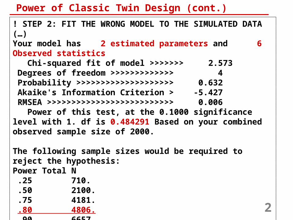
! STEP 2: FIT THE WRONG MODEL TO THE SIMULATED DATA(…)Your model has 2 estimated parameters and 6 Observed statistics Chi-squared fit of model >>>>>>> 2.573 Degrees of freedom >>>>>>>>>>>>> 4 Probability >>>>>>>>>>>>>>>>>>>> 0.632 Akaike's Information Criterion > -5.427 RMSEA >>>>>>>>>>>>>>>>>>>>>>>>>> 0.006 Power of this test, at the 0.1000 significance level with 1. df is 0.484291 Based on your combined observed sample size of 2000.

The following sample sizes would be required to reject the hypothesis: Power Total N .25 710. .50 2100. .75 4181. .80 4806. .90 6657. .95 8413. .99 12259. 2


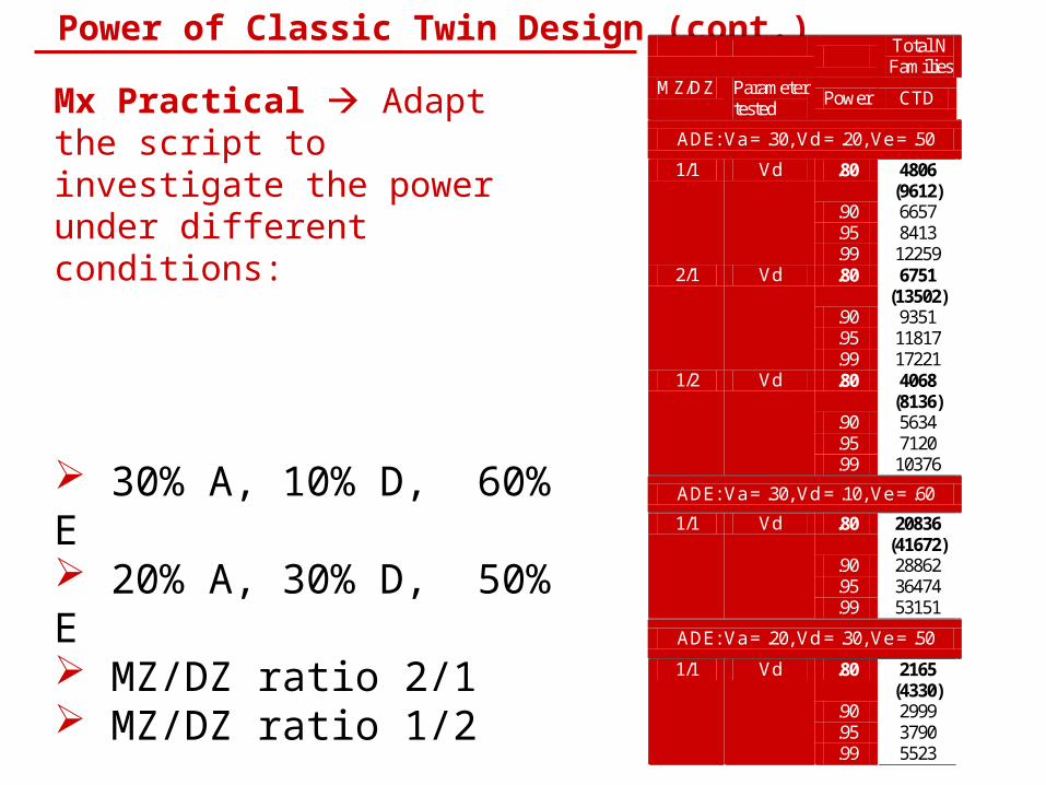
Mx Practical Adapt the script to investigate the power under different conditions:

30% A, 10% D, 60% E 20% A, 30% D, 50% E MZ/DZ ratio 2/1 MZ/DZ ratio 1/2

Total N Families

MZ/DZ Parameter tested

Power CTD

ADE: Va = .30, Vd = .20, Ve = .50

.80 4806 (9612)

.90 6657

.95 8413

1/1 Vd

.99 12259

.80 6751 (13502)

.90 9351

.95 11817

2/1 Vd

.99 17221

.80 4068 (8136)

.90 5634

.95 7120

1/2 Vd

.99 10376

ADE: Va = .30, Vd = .10, Ve = .60

.80 20836 (41672)

.90 28862

.95 36474

1/1 Vd

.99 53151

ADE: Va = .20, Vd = .30, Ve = .50

.80 2165 (4330)

.90 2999

.95 3790

1/1 Vd

.99 5523

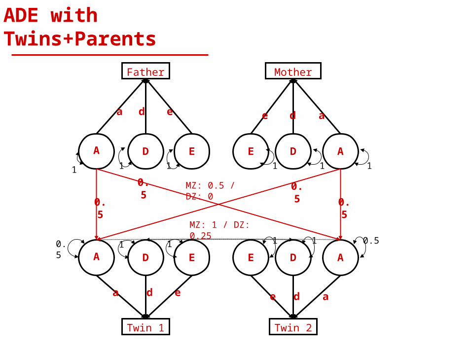
ADE with Twins+Parents

A D E

Twin 1

E D A

Twin 2

MZ: 1 / DZ: 0.25

Father Mother

A D E E D A

a d e ade

a d e ae d

0.5

0.5

0.5 0.

5

10.5 1 11 0.5

1 1 1 111

MZ: 0.5 / DZ: 0

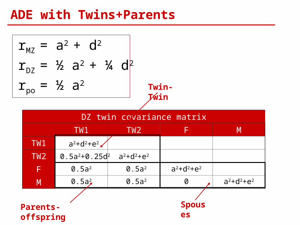
ADE with Twins+Parents

DZ twin covariance matrix

TW1 TW2 F M

TW1

TW2

F

M

rMZ = a2 + d2

rDZ = ½ a2 + ¼ d2

rpo = ½ a2

0.5a2+0.25d2

a2+d2+e2

a2+d2+e2

Twin-Twin

0.5a2

0.5a2 0.5a2

0.5a2

Parents-offspring

a2+d2+e2

a2+d2+e20

Spouses

Power of EFD: Twins + Parents

Mx Script powerADEtwins+parents.mx! Step 1: Simulate the data for power calculation of ADE model! 30% additive genetic (.5477²=.3)! 20% Non Additive genetic (.4472²=.2)! 50% random environment (.7071²=.5)


X Lower 1 1 Fixed ! genetic structureW Lower 1 1 Fixed ! non-additive genetic structureZ Lower 1 1 Fixed ! specific environmental structureH Full 1 1Q Full 1 1O Zero 1 1

End Matrices; 1

Power of EFD: Twins + Parents (cont.)


End Algebra; End


Covariances A+D+E | A+D | H@A | H@A _ A+D | A+D+E | H@A | H@A _

H@A | H@A | A+D+E | O _ H@A | H@A | O | A+D+E ;

Options MX%E=mzsim.covEnd 2



End Algebra; End


Covariances A+D+E | A+D | H@A | H@A _ A+D | A+D+E | H@A | H@A _


Options MX%E=mzsim.covEnd 2

Twin-Twin

Parent-offspring

Spouses

Twin 1 Twin 2 Father Mother


G3: DZ twin pairs Calculation NInput_vars=2 Matrices= Group 1 Covariances A+D+E | H@A+Q@D | H@A | H@A _

H@A+Q@D | A+D+E | H@A | H@A _ H@A | H@A | A+D+E | O _

H@A | H@A | O | A+D+E ;Options MX%E=dzsim.covEnd 3

!___________________________! Step 2: Fit the wrong model to the simulated data


X Lower 1 1 Free W Lower 1 1 FixedZ Lower 1 1 FreeH Full 1 1Q Full 1 1O Zero 1 1

End Matrices; Matrix H .5 Matrix Q .25


Begin Algebra;A= X*X' ;D= w*w' ;E= Z*Z' ;

End Algebra; End

G2: MZ twin pairs Data NInput_vars=4 Observations=1000 CMatrix Full File=mzsim.cov Matrices= Group 1

Covariances A+D+E | A+D | H@A | H@A _A+D | A+D+E | H@A | H@A _H@A | H@A | A+D+E | O _H@A | H@A | O | A+D+E ;Option RSidualsEnd4 5


G3: DZ twin pairs Data NInput_vars=4 NObservations=1000 CMatrix Full File=dzsim.cov

Matrices= Group 1

Covariances A+D+E | H@A+Q@D | H@A | H@A _ H@A+Q@D | A+D+E | H@A | H@A _


Start .5 AllOptions RSiduals Power= .01,1 ! for 1 tailed .05 probability value & 1 dfEnd 6

Mx Script powerADEtwins+parents.mxo


Your model has 2 estimated parameters and 20 Observed statistics Chi-squared fit of model >>>>>>> 43.582 Degrees of freedom >>>>>>>>>>>>> 18 Probability >>>>>>>>>>>>>>>>>>>> 0.001 Akaike's Information Criterion > 7.582 RMSEA >>>>>>>>>>>>>>>>>>>>>>>>>> 0.030 Power of this test, at the 0.0500 significance level with 1. df is 0.999998 Based on your combined observed sample size of 2000. The following sample sizes would be required to reject the hypothesis: Power Total N .25 166. .50 304. .75 485. .80 536. .90 683. .95 817. .99 1103.

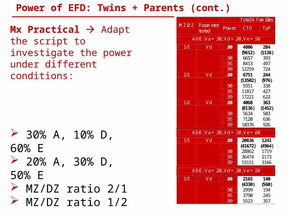
Mx Practical Adapt the script to investigate the power under different conditions:

30% A, 10% D, 60% E 20% A, 30% D, 50% E MZ/DZ ratio 2/1 MZ/DZ ratio 1/2

Power of EFD: Twins + Parents (cont.) Total N Families MZ/DZ Parameter

tested Power CTD TpP

ADE: Va = .30, Vd = .20, Ve = .50

.80 4806 (9612)

284 (1136)

.90 6657 393

.95 8413 497

1/1 Vd

.99 12259 724

.80 6751 (13502)

244 (976)

.90 9351 338

.95 11817 427

2/1 Vd

.99 17221 622

.80 4068 (8136)

363 (1452)

.90 5634 503

.95 7120 636

1/2 Vd

.99 10376 926

ADE: Va = .30, Vd = .10, Ve = .60

.80 20836 (41672)

1241 (4964)

.90 28862 1719

.95 36474 2173

1/1 Vd

.99 53151 3166

ADE: Va = .20, Vd = .30, Ve = .50

.80 2165 (4330)

140 (560)

.90 2999 194

.95 3790 245

1/1 Vd

.99 5523 357

Assumptions and limitations

The model assumes no generational differences in the variance components

The use of a scalar can help to solve a difference in the total variance

Measurement issue: Same instrument for parents and offspring?

Implementing the model becomes more problematic with complex models: e.g. GxE

Dominance and Contrast effects might be confounded: Beware of variance differences between MZs and DZs

Mx Practical, Real Data: Dominance in TAB

The complete sample consists of 1670 families

Mx Practical, Real Data: Matrices

Mx Script TAB_ADE.mx

Males Females Others

X=[a], A=[a2]

W=[d], D=[d2]

Z=[e], E=[e2]

J=[a], T=[a2]

Y=[d], U=[d2]

L=[e], V=[e2]

H=[0.5]

Q=[0.25]

S=[γ]: Scalar

F=[0]: Spouse correlation

G=[mT mT mF mM]: Means

R = A+D+E | A+D | H@A | H@(X*J') _ A+D | A+D+E | H@A | H@(X*J') _

H@A | H@A | A+D+E | F _ H@(J*X')| H@(J*X') | F | T+U+V ;

MZM TwinM-TwinM

Parents-offspring Spouses



X=[a], A=[a2]

W=[d], D=[d2]

Z=[e], E=[e2]

J=[a], T=[a2]

Y=[d], U=[d2]

L=[e], V=[e2]

H=[0.5]

Q=[0.25]

S=[γ]: Scalar



R = T+U+V | H@T+Q@U | H@(J*X')| H@T _ H@T+Q@U | T+U+V | H@(J*X')| H@T _ H@(X*J') | H@(X*J') | A+D+E | F _ H@T | H@T | F | T+U+V ;

DZF TwinF-TwinF


R = A+D+E | H@(X*J')+Q@(W*Y') | H@A | H@(X*J') _ H@(J*X')+Q@(Y*W') | T+U+V | H@(J*X') | H@T _ H@A | H@(X*J') | A+D+E | F _ H@(J*X') | H@T | F | T+U+V ;

OSMF TwinM-TwinF




X=[a], A=[a2]

W=[d], D=[d2]

Z=[e], E=[e2]

J=[a], T=[a2]

Y=[d], U=[d2]

L=[e], V=[e2]

H=[0.5]

Q=[0.25]

S=[γ]: Scalar




Matrix B (dot) multiplies Matrix R:

The Twin-Twin covariance is unaffected

Then Parent-Twin covariance is multiplied by γ

The Parent-Parent covariance is multiplied by γ2

22

22

11

11

11

11

B

N

S

Twin-Twin

Parent-Twin Parent-Parent

Scalar Matrix B= N | (N@S)_ (N@S) | (N@(S*S'));

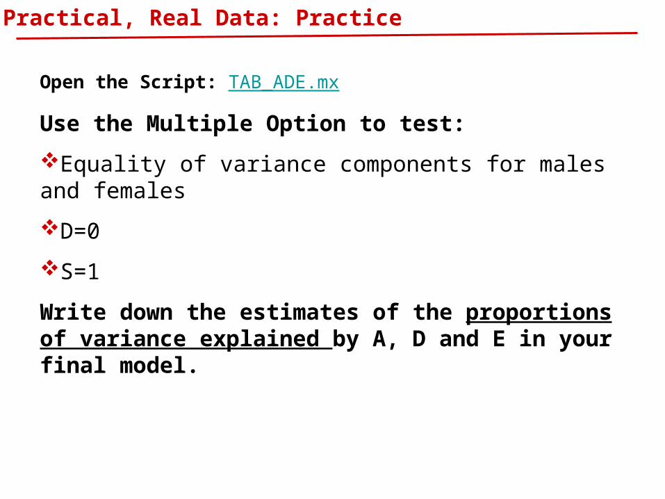
Mx Practical, Real Data: Practice

Open the Script: TAB_ADE.mx

Use the Multiple Option to test:

Equality of variance components for males and females

D=0

S=1

Write down the estimates of the proportions of variance explained by A, D and E in your final model.

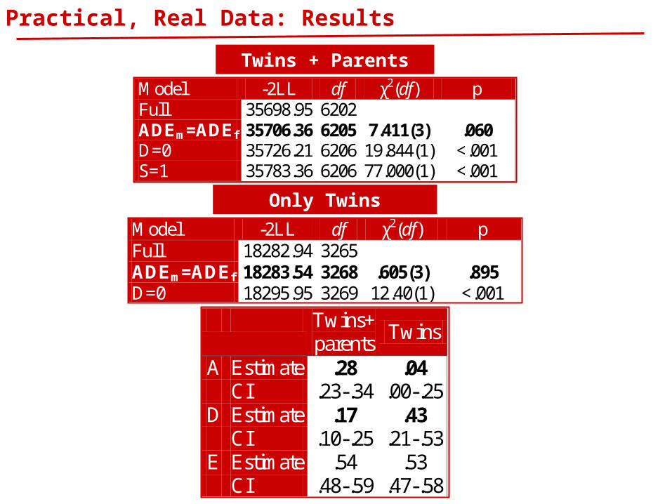
Mx Practical, Real Data: Results

Twins + Parents

Only Twins

Model -2LL df χ2(df) p Full 35698.95 6202 ADEm=ADEf 35706.36 6205 7.411(3) .060 D=0 35726.21 6206 19.844(1) <.001 S=1 35783.36 6206 77.000(1) <.001

Model -2LL df χ2(df) p Full 18282.94 3265 ADEm=ADEf 18283.54 3268 .605(3) .895 D=0 18295.95 3269 12.40(1) <.001

Twins+ parents

Twins

A Estimate .28 .04 CI .23-.34 .00-.25 D Estimate .17 .43 CI .10-.25 .21-.53 E Estimate .54 .53 CI .48-.59 .47-.58

Genetic Dominance in Extended Pedigrees: Boulder, March 2008 Irene Rebollo Biological Psychology...

Documents

Transcript of Genetic Dominance in Extended Pedigrees: Boulder, March 2008 Irene Rebollo Biological Psychology...