Genetic Assessment of Gopher Frog Populations in...
47
Genetic Assessment of Gopher Frog Populations in Florida Final Report KEVIN M. ENGE, Principal Investigator Florida Fish and Wildlife Conservation Commission, Fish and Wildlife Research Institute, Lovett E. Williams, Jr. Wildlife Research Laboratory, 1105 SW Williston Road, Gainesville, Florida 32601 Co-Principal Investigators: THOMAS J. DEVITT Center for Computational Biology and Bioinformatics, The University of Texas at Austin, 1 University Station #C0930, Austin, TX 78712 ANNA L. FARMER Florida Fish and Wildlife Conservation Commission, Fish and Wildlife Research Institute, Lovett E. Williams, Jr. Wildlife Research Laboratory, 1105 SW Williston Road, Gainesville, Florida 32601 STACEY LANCE University of Georgia, Savanna River Ecology Laboratory, PO Drawer E, Aiken, South Carolina 29802 STEPHEN C. RICHTER Eastern Kentucky University, Department of Biological Sciences, 521 Lancaster Avenue, Richmond, Kentucky 40475 PETER BEERLI Florida State University, Department of Scientific Computing, Tallahassee, Florida 32306 Florida State Wildlife Grants Project ID 9272 251 1159 Dates Covered: July 1, 2013 – December 31, 2016 Date Submitted: February 1, 2017
Transcript of Genetic Assessment of Gopher Frog Populations in...
Genetic Assessment of Gopher Frog Populations in Florida
Final Report
KEVIN M. ENGE, Principal Investigator Florida Fish and Wildlife Conservation Commission, Fish and Wildlife Research Institute, Lovett
E. Williams, Jr. Wildlife Research Laboratory, 1105 SW Williston Road, Gainesville, Florida 32601
Co-Principal Investigators:
THOMAS J. DEVITT Center for Computational Biology and Bioinformatics, The University of Texas at Austin, 1 University
Station #C0930, Austin, TX 78712
ANNA L. FARMER Florida Fish and Wildlife Conservation Commission, Fish and Wildlife Research Institute, Lovett
E. Williams, Jr. Wildlife Research Laboratory, 1105 SW Williston Road, Gainesville, Florida 32601
STACEY LANCE University of Georgia, Savanna River Ecology Laboratory, PO Drawer E, Aiken,
South Carolina 29802
STEPHEN C. RICHTER Eastern Kentucky University, Department of Biological Sciences, 521 Lancaster Avenue,
Richmond, Kentucky 40475
PETER BEERLI Florida State University, Department of Scientific Computing, Tallahassee, Florida 32306
Florida State Wildlife Grants Project ID 9272 251 1159
Dates Covered: July 1, 2013 – December 31, 2016
Date Submitted: February 1, 2017

Enge et al. Gopher Frog Genetics
ABSTRACT
Florida represents the last stronghold for the gopher frog, Rana (=Lithobates) capito, which has experienced serious declines in the rest of its range. Florida gopher frog populations have also experienced declines, particularly in the panhandle, primarily due to habitat degradation and reduction of gopher tortoise (Gopherus polyphemus) populations. Understanding gene flow and genetic diversity is necessary to determine whether populations will remain viable over time and whether additional management actions are needed in cases where populations have become isolated due to manmade barriers. The first objective of this study was to determine the amount of gene flow and degree of genetic variation among populations in 15 different geographical locations of known or suspected occupancy (areas of occupancy or AOs) that may be genetically isolated by natural or manmade barriers. We collected a total of 1,748 samples from 127 ponds in 14 of the 15 primary AOs and all 5 alternate AOs. We achieved our goal of collecting 30 samples from 10 of the primary AOs and 2 of the alternate AOs. The second objective was to examine rates of gene flow and genetic variation among breeding ponds within the same AO by collecting ≥30 genetic samples from at least 4 ponds in 3 AOs, which we achieved. A total of 1,191 samples from 64 ponds on 27 properties was genotyped across 10 microsatellite loci. Genetic diversity is high; an analysis of molecular variance indicated that the within-population component of genetic variation contributes 82% of total genetic diversity. Fixation index (FST) values are low, indicating weak genetic population structure. Population clustering analyses in Structure identified panhandle and peninsular populations as 2 genetic clusters separated by the low-lying region near the Aucilla River. The panhandle and peninsular genetic clusters correspond with the Coastal Plain and peninsular lineages identified previously using mitochondrial DNA, but we failed to detect a genetic break in the peninsula. Geneland analyses identified 26–31 genetic clusters, indicating further substructure on a regional scale. Analysis of historical migration indicated an east-west population divergence event followed by immigration to the east (i.e., from the panhandle to the peninsula). We examined migration over the last several generations in 2 regions, Ocala National Forest and Jennings State Forest/Camp Blanding Military Reservation. This and an earlier genetic study suggest that the panhandle and peninsular subpopulations should be considered different management units. The panhandle (i.e., Coastal Plain) lineage probably warrants state and federal listing as Threatened because of population declines.
" 2

Enge et al. Gopher Frog Genetics
ACKNOWLEDGMENTS
Support for the project was provided by the Florida Fish and Wildlife Conservation Commission’s Florida Wildlife Legacy Initiative and the U.S. Fish and Wildlife Service’s State Wildlife Grants program “Data Gaps Projects Grant Cycle 2012, T-30.” Grant assistance was provided by Andrea Alden, Ginger Gornto, and Robyn McDole. Jamie Barichivich, Glenn Bartolotti, Bob Simons, Travis Blunden, Jim Blush, Joe Burgess, Brian Camposano, Garrett Craft, Jason DePue, Nancy Dwyer, Erik Egensteiner, Carolyn Enloe, Mel Gramke, Christopher Haggerty, Allan Hallman, Stephen Harris, Emma Knight, Joe Mansuetti, Jonathan Mays, Ryan Means, Paul Moler, Vince Morris, Dwight Myers, Jennifer Myers, Charlie Pedersen, Ralph Risch, Jonathan Roberts, Emily Rushton, Carrie Sekerak, Sarah Reintjes-Tolen, Jordan Schmitt, Jen Stabile, Travis Thomas, Courtney Tye, Lindsay Wagner, and Graham Williams helped collect genetic samples.
" 3
Enge et al. Gopher Frog Genetics
TABLE OF CONTENTS
Abstract…………………………………………………………….………………………….…. 2
Acknowledgments……………………………………………………………………………….. 3
Introduction………………………………………………………………………………………. 5
Methods………………………………………………………………………………………...… 7
Sample Collection……………………………………………………………………………. 7
Molecular Methods…………………………………………………………………………… 7
Data Analysis…………………………………………………………………………………. 8
Results …………………………………………………………………………………………… 10
Objective 1………………………………………………………………………………….. 10
Sample collection and genotyping………………………………………………………. 10
Microsatellite descriptive statistics……………………………………………………… 10
Relatedness……………………………………………………………………………… 10
Analysis of molecular variance (AMOVA)……………………………………………... 10
Clustering analyses……………………………………………………………………… 11
Analysis of migration…………………………………………………………………… 11
Objective 2….……………………………………………………… ……....………………. 11
Discussion……………………………………………………………………………………….. 12
Conclusions……………………………………………………………………………………… 14
Literature Cited………………………………………………………………………………….. 15
" 4

Enge et al. Gopher Frog Genetics
INTRODUCTION
Florida represents the last stronghold for the gopher frog, Rana (=Lithobates) capito, which has experienced serious declines in the rest of its range (Jensen and Richter 2005). Even in Florida, populations have declined in some areas, and relatively few extant populations are known from the panhandle (Enge et al. 2014). The U.S. Fish and Wildlife Service was petitioned to list the gopher frog as a Threatened species in 2012 (Adkins Giese et al. 2012) and is currently evaluating its status to determine if it warrants listing. At the state level, the gopher frog is currently designated a Species of Greatest Conservation Need (FWC 2012) and was previously listed as a Species of Special Concern. A biological status review determined that the gopher frog failed to meet criteria for continued listing as a state imperiled species, but upland and wetland habitat loss and fragmentation were identified as significant threats (FWC 2011). In November 2016 after approval of an imperiled species management plan, the gopher frog was delisted in Florida, but it is still protected from take.
Although telemetry studies of individual gopher frog populations have been conducted in Florida (Blihovde 2006, Roznik et al. 2009), little information exists regarding the level of connectivity and gene flow among populations in different parts of the state. Areas of unsuitable habitats limit gene flow and result in genetic differences among populations. Over long timescales, natural barriers and selection pressure can result in the local adaptation of populations (Slatkin 1987).
Habitat fragmentation from roads, urban areas, agriculture, and silviculture has been demonstrated to negatively impact genetic diversity in amphibian populations (Allentoft and O’Brien 2010). In general, amphibians are vulnerable to habitat fragmentation due to their relatively low dispersal ability, naturally low effective population sizes, and tendency to exist in metapopulations where periodic local extinctions are common and dispersal from neighboring populations plays a key role in reestablishing populations (Allentoft and O’Brien 2010); this is particularly true for the gopher frog (Greenberg 2001, reviewed by Richter et al. 2009). When habitats become fragmented and barriers reduce or eliminate gene flow among populations, isolated populations may experience a reduction in genetic diversity through the processes of genetic drift and inbreeding, resulting in decreased fitness and lack of adaptability to a changing environment (Amos and Balmford 2001, Allentoft and O’Brien 2010). Reduced genetic diversity in amphibian populations has been linked to reductions in fitness-related traits, including decreased survival, decreased reproductive success and larval growth, increased physical abnormalities, and increased susceptibility to disease and pollutants (Allentoft and O’Brien 2010). As a result, the likelihood of local and regional extinction is higher when small amphibian populations become isolated by anthropogenic barriers (Cushman 2006, Richter et al. 2009, Allentoft and O’Brien 2010). Understanding gene flow and genetic diversity is necessary to determine whether populations will remain viable over time and whether additional management actions are needed in cases where populations have become isolated due to anthropogenic barriers.
The gopher frog is a gopher tortoise (Gopherus polyphemus) commensal that is commonly encountered when tortoises are translocated from development sites. Until recently,
" 5

Enge et al. Gopher Frog Genetics
FWC policy has allowed the gopher frog and other commensal species to be translocated with tortoises from development sites to recipient sites, but this policy has been temporarily halted until the effects of translocations can be studied. If natural genetic differences are not maintained when animals are moved among populations, outbreeding depression can occur, resulting in reduced fitness to the new environment or reduced fitness from the disruption of coadapted gene complexes in offspring (Moritz 1999). This study provides information on the levels of historical and recent gene flow and the degree of genetic differentiation of Florida populations, enabling the identification of both genetically distinct populations as well as historical barriers between populations. This information will aid in understanding the genetic diversity of the species and enable FWC staff to make informed decisions regarding the genetic consequences of translocating this commensal species.
A range-wide genetic study of the gopher frog by Richter et al. (2014) using mitochondrial DNA (mtDNA) identified a Coastal Plain lineage including the Florida panhandle and 2 peninsular Florida lineages, although the exact locations of genetic breaks could not be identified because of insufficient sampling coverage. The Coastal Plain lineage was estimated to have diverged 1.9–2.3 million years ago (mya), and the northern and southern peninsular lineages diverged 1.1–1.3 mya, depending on the mutation rate used (Richter et al. 2014). The lineages recovered did not follow geographic boundaries of previously recognized subspecies, supporting Young and Crother’s (2001) recommendation that these subspecific designations of gopher frogs be disregarded.
This project aimed to fill data gaps that were identified as a key conservation challenge for the gopher frog in Florida’s State Wildlife Action Plan (FWC 2012; p. 8). Florida’s Wildlife Legacy Initiative (FWLI) has a data gaps goal of moving 10 priority SGCN up at least 1 “knowledge level” by 2017 (FWLI website). Because the taxonomy of peninsular populations has not been determined, the current knowledge level of the gopher frog could be considered to be level 0 (status of the taxon is unknown). Once the taxonomy is determined, the gopher frog’s knowledge level will be 4 (if the taxon is known or thought to be declining or the population is low, we know why). Results from this study on genetic diversity and rates of recent and historical gene flow among populations across the state will inform a taxonomic study of this species, as well as allow us to better understand the long-term viability of populations and to identify populations that may require additional management actions. We will be able to provide sound management recommendations for declining populations, increasing the knowledge level to 5 (if the taxon's population is low or declining and we know why, we know what is needed to develop management recommendations to improve population status). Information gathered by this study on the genetic connectivity and viability of populations in Florida will also be useful in determining whether this species requires additional state or federal protection.
The objectives of this study were to:
Objective 1 – Determine the amount of gene flow and degree of genetic variation among gopher frog populations in different geographical locations of known or suspected occupancy (hereafter referred to as areas of occupancy or AOs) in Florida that may be genetically isolated by natural
" 6

Enge et al. Gopher Frog Genetics
or manmade barriers. To do this, 30–35 genetic samples were to be collected and analyzed from at least 1 breeding pond in each of 15 AOs across the state.
Objective 2 – Examine rates of gene flow and genetic variation among breeding ponds within the same area of occupancy. To do this, 30–35 genetic samples were to be collected and analyzed from 3−5 breeding ponds within 2 or 3 different AOs.
METHODS
Sample Collection
Using known localities for gopher frogs in Florida (Krysko et al. 2011, Enge et al. 2014), we identified all locations with recent records (since 1990) and locations with historical records that are suspected to have extant populations due to the continued occurrence of suitable habitat (Fig. 1). Based on a map of potentially extant populations, we identified 20 spatially distinct areas of occupancy (Fig. 2). These areas of occupancy may be genetically isolated from adjacent areas by natural barriers, such as rivers or unsuitable habitat, or by manmade barriers: interstates, canals, urban areas, or other unsuitable, human-modified habitats. For this study, we divided these areas of occupancy into 15 primary and 5 alternate sites (Fig. 2), where alternate sites are those areas that are less likely to have robust gopher frog populations because of degraded habitat or lack of known breeding ponds. If areas of occupancy are genetically isolated, they may represent different management units. To investigate the degree of genetic isolation and genetic diversity among these areas (Objective 1), FWRI staff tried to collect 30–35 genetic samples from at least 1 breeding pond in each of the 15 primary areas of occupancy. If insufficient sample sizes were obtained from the 15 primary areas, we attempted to collect at least 30 samples from alternate areas. Potential sampling sites within each area of occupancy are identified in Table 1. To examine the genetic variation and gene flow within areas of occupancy (Objective 2), 2 or 3 of the 15 areas sampled for Objective 1 were selected for more intensive sampling. Genetic samples from 30–35 individuals were collected from 3–5 breeding ponds in these additional areas and analyzed to determine the amount of gene flow and genetic variation among ponds within the same area.
All sample collections occurred during Years 1–2 of the project. Gopher frog tissue collection was conducted in collaboration with land managers and biologists on public lands and with permission from landowners on private lands. Gopher frogs were captured for tissue collection primarily by dipnetting tadpoles from ponds and removing their tail tips. In a few instances, tissue samples were collected by clipping a single toe from metamorphic gopher frogs. Tissue samples were immediately stored in 95% ethanol in individually marked cryogenic vials until genetic analysis.
Genotyping
DNA was extracted from tissues using standard methods, and 10 microsatellite loci were amplified and genotyped following the protocol of Nunziata et al. (2012). Microsatellites are
" 7

Enge et al. Gopher Frog Genetics
short, tandemly repeated loci in eukaryotic genomes that are used widely in population genetic studies because they are often highly polymorphic and easy to survey (Ellegren 2004). Microsatellites allow for the characterization of population structure, including estimates of gene flow, migration rates, and times since population divergence, as well as levels of genetic diversity (allelic richness, levels of heterozygosity, etc.). Microsatellites have been widely used to study gene flow in amphibians (Jehle and Arntzen 2002, Beebee 2005).
Dr. Stacey Lance conducted molecular genetic labwork at the University of Georgia’s Savannah River Ecology Laboratory (SREL), Aiken, South Carolina. She developed a multiplex approach set for the gopher frog PCRs that allowed running of more than 1 locus in each reaction, which reduced the cost per sample by requiring fewer plates of PCR and fragment analysis. However, this multiplex approach failed to work consistently enough to continue using. Instead, costs were reduced by using the less expensive and more efficient Chelex solution for DNA extraction, which allowed genotyping of 299 more samples than specified in the contract.
Data Analysis
Dr. Thomas Devitt conducted statistical analyses of the genetic data. Sample sizes were uneven among ponds (mean 19, range 1−35; Table 2). To overcome any bias due to small or uneven sample sizes among ponds, analyses were performed on the entire dataset as well as a subset of the data consisting only of those ponds with at least 30 sampled individuals (762 individuals from 25 ponds).
Each sampled pond was treated as a population a priori for calculating basic genetic diversity and differentiation statistics, because that is the lowest level of genetic structure we would expect based on the life history of this species (i.e., a deme). We used Genepop (Raymond and Rousset 1995, Rousset 2012) to calculate allele frequencies, observed and expected genotype counts, exact tests for Hardy–Weinberg (HW) genotypic equilibrium, estimates of null allele frequencies (Brookfield 1996), exact G-tests of population differentiation based on allelic frequencies (Goudet et al. 1996), F-statistics based on allele identity (Cockerham 1973, Weir and Cockerham 1984), and F-statistic analogs for microsatellites based on allele size (Rousset 1996) using the method of Michalakis and Excoffier (1996). Significance was assessed using Markov chain Monte Carlo (MCMC) simulation (Guo and Thompson 1992) with default values for the Markov chain (100 batches with 1000 iterations per batch and 1000 dememorization steps). Additional population differentiation estimators were calculated using GenoDive (Meirmans and Van Tienderen 2004), including Nei’s GST (Nei 1973), Hedrick’s (2005) standardized fixation index (G’ST), Meirmans and Hedrick’s (2011) estimator (G”ST) and Jost’s D (Jost 2008). Standard deviations for these population differentiation estimators were obtained by jackknifing over loci, and 95% confidence intervals through bootstrapping over loci in GenoDive. Allelic richness (rarefied allelic counts [Hurlbert 1971, El Mousadik and Petit 1996]) was calculated per locus and population for ponds with at least 30 samples using the hierfstat package for R (Goudet 2005). We tested for a correlation between the total number of alleles and differentiation estimators to assess the degree of polymorphism bias on diversity statistics using the diveRsity package for R (Keenan et al. 2013). Finally, because individuals
" 8

Enge et al. Gopher Frog Genetics
sampled from the same pond may be siblings, we tested for relatedness within ponds using Queller and Goodnight’s (1989) estimator implemented in GenAlEx (Peakall and Smouse 2006 2012).
We analyzed overall population structure using 2 approaches. First, we performed an analysis of molecular variance (AMOVA; Excoffier et al. 1992) to quantify within-population and among-population genetic diversity. We performed 10,100 permutations to test the significance of the variance components and their associated F-statistic analogs under an infinite allele model implemented in GenoDive.
Second, we used individual-based assignment methods for inferring population structure implemented in Structure and Geneland (Guillot et al. 2005, 2008). In Structure, we examined values of K (the number of populations) from 1 to 25. Because Structure may be influenced by small sample sizes (Evanno et al. 2005), we analyzed both the full dataset and a subset of the data containing only populations with at least 30 samples. This reduced dataset comprised 732 individuals from 25 subpopulations (Fig. 3). We examined values of K from 1 to 15 for the reduced dataset. Null alleles (population-specific double missing genotypes) were coded as missing. We used the correlated allele frequency model and assumed admixture among populations using the default settings. Analyses were performed both with and without sample group information as a prior (Hubisz et al. 2009). Ten runs were conducted for each value of K in Structure, with each run consisting of 50,000 steps after a burn-in of 10,000 steps. We chose this burn-in value and assessed MCMC convergence by examining time series plots of key parameters (𝛼, F, likelihood) along the run. We evaluated the “best” K by examining Evanno’s (2005) ΔK method as well as the log probability of the data (lnPr(X|K)) following the software authors’ recommendation (Structure manual section 5.3) using the web program Structure Harvester (Earl and vonHoldt 2011). Results were summarized and visualized using Clumpp (Jakobsson and Rosenberg 2007) and Distruct (Rosenberg 2004) implemented in the web program Clumpak (Kopelman et al. 2015) or the R package pophelper.
In Geneland, we assumed correlated allele frequencies under a spatial model and assumed no admixture (the only option implemented for more than 2 populations). We examined values of K from 1 to 50. The frequency of null alleles was estimated, and it was filtered if the frequency was >10% (Guillot et al. 2008). Five independent runs were conducted, with each run consisting of 100,000 steps following a burn-in of 20,000 steps. MCMC convergence was examined using postprocessing functions implemented in the R graphical user interface for the program (Guillot et al. 2005).
We estimated historical migration (on the order of thousands of years ago) across a genetic discontinuity between panhandle and peninsular populations separated by the Aucilla River that was identified by preliminary Structure analyses as well as by Richter et al. (2014) using mtDNA sequence data. Five subpopulations (sampled ponds) with at least 20 individuals each were pooled into 2 ‘populations’: panhandle (ponds EAFB101, ANFCL007, and ANF003) and peninsula (BBSCU and FWMP008; Fig. 4). We tested 7 models that specify different population histories (Fig. 4) using the software Migrate 4.2.9 (Beerli and Palczewski 2010) to evaluate the different models based on their marginal likelihood. Migrate uses Bayesian
" 9

Enge et al. Gopher Frog Genetics
inference to calculate the probability of explicit population models in a coalescent framework. The null hypothesis (and simplest case) is that sampled ponds belong to a single (panmictic) population (model 7). More complex models include a divergence event (models 1, 2, and 6) and various directional migration scenarios (e.g., immigration to the east only, east and west, west only, etc.).
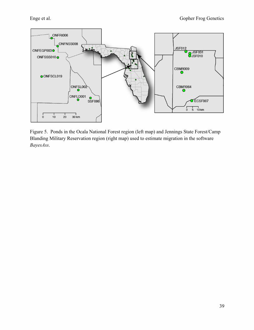
We also examined migration on a more recent timescale (over the last several generations) using a different approach implemented in the software BayesAss 3.0 (Wilson and Rannala 2003). We focused on 2 regions where our sampling is relatively dense, Ocala National Forest and Jennings State Forest/Camp Blanding Military Reservation (Fig. 5). These regions were selected because they contain ponds with sufficient sample sizes that are not separated by any obvious geographic barriers other than distance alone (1–23 km between ponds). We adjusted mixing parameters until acceptance rates for proposed changes to migration rates, allele frequencies, and inbreeding coefficients were between 20% and 60%. We conducted 2 runs initialized with different seeds and compared the posterior mean parameter estimates to check for convergence following the software author’s recommendation.
" 10
Enge et al. Gopher Frog Genetics
RESULTS
Objective 1
Sample collection and genotyping.—We collected a total of 1,748 samples, primarily gopher frog tadpole tail tips, from 127 ponds in 14 of the 15 primary AOs and all 5 alternate AOs (Table 1). The availability of samples was contingent upon ponds filling and the availability of tadpoles. We were unable to find gopher frogs at Pumpkin Hill Creek Preserve State Park, Nassau County (AO Alt #5), but we found the first gopher frogs in Cary State Forest, Duval County, which we are considering as being part of this AO. The number of samples ranged from 0 in AO #6 to 420 in AO #5 (Table 1). We failed to collect any samples from AO #6 along the Atlantic Coast, despite sampling Faver-Dykes State Park, St. Johns County. Several trips to potential or known gopher frog ponds in AO #2 (Bay, Washington, Calhoun, and Jackson counties) yielded only 3 samples from 1 pond in Calhoun County. We achieved the goal of collecting 30 samples from 10 of the primary AOs and 2 of the alternate AOs. We collected >20 samples, which is an acceptable though not ideal number for our genetic analyses, from 13 of the primary AOs and 3 of the alternate AOs (Table 1). Dr. Stacey Lance genotyped across 10 microsatellite loci 1,191 of 1,428 samples that she received.
" 11

Enge et al. Gopher Frog Genetics
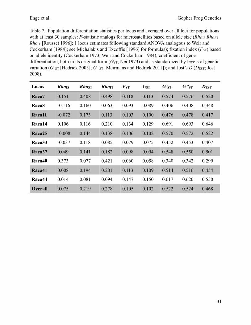
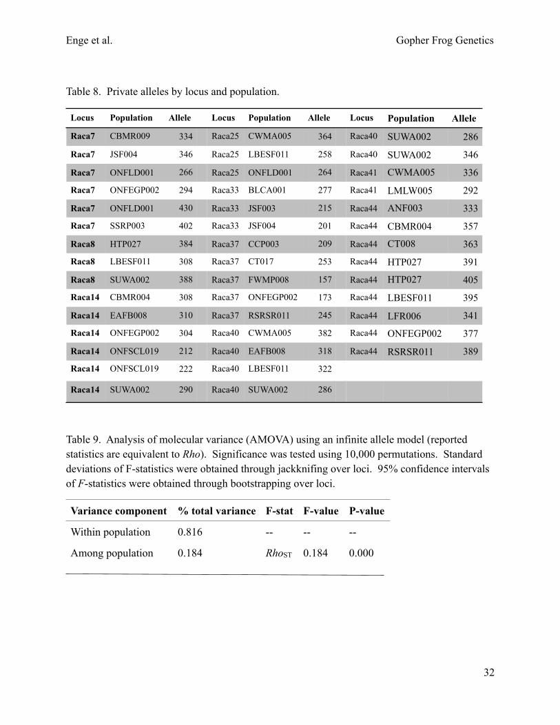
Microsatellite descriptive statistics.—Dr. Thomas Devitt conducted microsatellite DNA analysis of 1,191 genotyped samples from 64 ponds. Summary statistics for populations with at least 30 samples are provided in tables 3–8. The mean number of alleles averaged over all loci and populations is 24 (Table 3, Fig. 6). The effective number of alleles (i.e., the number of alleles weighted by their frequency) is 5 (Table 3). Heterozygosity and gene diversity estimates are high (mean 0.8; tables 3–5). Allelic differentiation among populations is significant based on exact G-tests (P < 0.001), allowing us to reject the hypothesis that alleles were drawn from the same distribution in all populations. We did not find a significant correlation between locus polymorphism and diversity partitioning statistics (Fig. 7; see Keenan et al. 2013). Heterozygosity-based tests for Hardy Weinberg equilibrium (GIS; Nei 1987) are significant (P < 0.05) for 15 of 25 populations with at least 30 samples (Table 6). Population differentiation statistics per locus and averaged over all loci for populations with at least 30 samples are shown in Table 7. Several populations have 1 or more private alleles (Table 8).
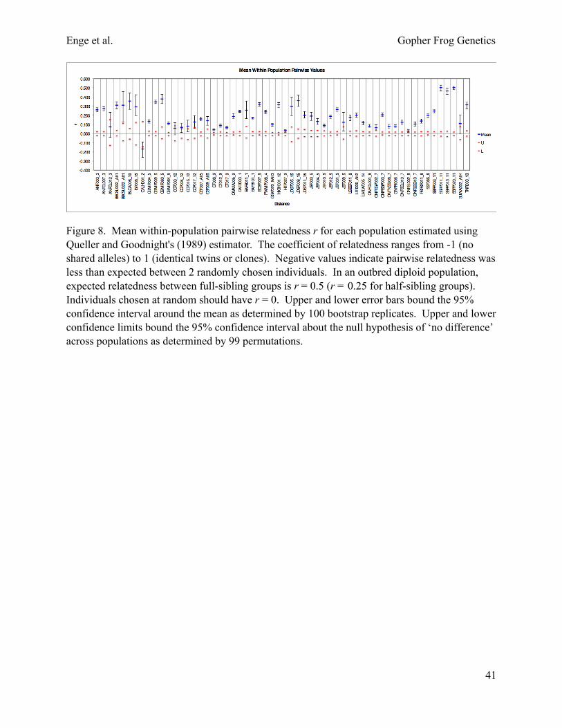
Relatedness.—Mean within-population pairwise relatedness r for each population estimated using Queller and Goodnight's (1989) estimator reveal several populations with a high mean within-population pairwise relatedness value (Fig. 8). Taking into account sample sizes and confidence limits on point estimates, St. Sebastian River Preserve State Park populations (SSRP003, SSRP011, and SSRP020) contain putative full-sibling groups (r = 0.5). Populations with putative half-sibling groups (r = 0.25) include Apalachicola National Forest populations (ANF003 and ANFCL007), Big Bend Wildlife Management Area’s Spring Creek Unit (BBSCU002), Camp Blanding Military Reservation (CBMR009), Eglin Air Force Base (EAFB003), Etoniah Creek State Forest (ECSF007), private land near Highlands Hammock State Park (HIGH001), and Jennings State Forest (JSF031). Other populations show a higher degree of relatedness than expected at random, but low sample sizes for some of these populations may bias relatedness estimates upwards.
Analysis of molecular variance (AMOVA).—AMOVA results are shown in Table 9. Within-population variation accounts for most (82%) of the total variance, with among-population variation capturing 18%.
Clustering analyses.—Time series plots of summary statistics and relevant parameters show MCMC convergence well before the 10,000 steps excluded as burn-in. Mean values of the tuning parameter r indicate that sample group is informative about ancestry (Hubisz et al. 2009). Our preferred model assumes admixture and correlated allele frequencies among populations, using sample group as prior information to assist clustering. Under this model, the mean log probability of the data is greatest for K = 17, though the rate of change in the log probability of the data (ΔK; Evanno et al. 2005) is greatest from 1 to 2 clusters, and nearly as great from 2 to 3 clusters (Fig. 9). At K = 2, panhandle populations cluster separately from peninsular populations. At K = 3, individuals from St. Sebastian River Preserve State Park (SSRP) form a third cluster. Removing the divergent panhandle populations from the analysis to explore further subdivision among peninsular populations (see Structure manual section 5.3) did not reveal additional structure within the peninsula; ΔK is greatest from 1 to 2 clusters, with the SSRP samples again forming a separate cluster. Removing either or both the divergent panhandle
" 12
Enge et al. Gopher Frog Genetics
populations and SSRP population from the analysis did not reveal additional structure within the peninsula; ΔK is greatest from 1 to 2 clusters (Fig. 9).
The effect of small sample sizes did not appear to change Structure results. For the subset of the data including only populations with at least 30 samples, the mean log probability of the data is greatest for K = 17, though the rate of change in the log probability of the data (ΔK; Evanno et al. 2005) is greatest from 1 to 2 clusters, and nearly as great from 2 to 3 clusters (not shown).
In Geneland, the number of clusters (K) ranges from 26–31 over 5 separate runs (Fig. 10). Differences in the number of clusters among runs appear to result from shared missing data (null alleles)
Analysis of migration.—For our analysis of historical migration, we tested 7 models that specify different population histories of panhandle and peninsular samples separated by the Aucilla River. Based on the model probabilities, the best model specifies an east-west population divergence event with immigration to the east (i.e., from the panhandle to the peninsula). All other tested models are improbable (Table 10).
Objective 2
This objective was to examine genetic variation at a finer scale using 3−5 ponds within 2 or 3 AOs. We exceeded our goal by collecting at least 30 samples from 4 ponds in AO #5 (Jennings State Forest, Camp Blanding Military Reservation, and Etoniah Creek State Forest), 8 ponds in AO #7 (Ocala National Forest), and 6 ponds in AO #9 (Annutteliga Hammock, Chassahowitzka Wildlife Management Area, Croom Tract of Withlacoochee State Forest, and Halpata Tastanaki Preserve). We have 92 samples (at least 30 samples from 2 ponds) from St. Sebastian River Preserve State Park (AO #11), which is bisected into quadrants (presumably 4 populations with no genetic exchange) by I-95 and the channelized St. Sebastian River. Where possible, we collected genetic samples from as many ponds as possible within an AO in order to gain a better understanding of population genetic structure at a fine scale.
We examined migration on a more recent timescale (over the last several generations) using the software BayesAss 3.0 (Wilson and Rannala 2003). We focused on 2 regions where we had sufficient sample sizes from ponds at variable distances: Jennings State Forest/Camp Blanding Military Reservation (Fig. 11) and Ocala National Forest (Fig. 12). In the Jennings State Forest/Camp Blanding region, the highest level of migration occurred between ponds JSF010 and JSF012 (Fig. 11); 0.222 individuals per generation in Pond JSF012 were migrants from Pond JSF010 (Table 11), despite being separated by 4.9 km and 1 large and 2 smaller tributaries of Black Creek. In contrast, very little migration occurred between ponds JSF010 and JSF031 (Fig. 11), which are only 1.8 km apart and separated by Wheeler Branch, a small tributary (100-m-wide floodplain) of Black Creek. Only 0.008 individuals per generation in Pond JSF010 were migrants from Pond JSF031 (Table 11). More migration occurred between ponds JSF012 and JSF031, which are 3.8 km apart and separated by a large tributary (≥300-m-wide floodplain) of Black Creek (Fig. 11). No significant migration occurred between Camp Blanding Military Reservation and Jennings State Forest or between Camp Blanding and Etoniah Creek State Forest (Pond ECSF007), all of which are separated by streams, 2-lane roads, and
" 13

Enge et al. Gopher Frog Genetics
some developed areas. Some migration occurred between ponds CBMR004 and CBMR064, which are separated by 8.8 km of contiguous sandhill habitat (Fig. 11); 0.180 individuals per generation in Pond CBMR004 were migrants from Pond CBMR064 (Table 11).
In the Ocala National Forest region, more migration typically occurred among ponds than in the Jennings State Forest/Camp Blanding region (Tables 11, 12). In the eastern portion of Ocala National Forest, migration occurred in a north-south direction between most of the 6 ponds (Table 12, Fig. 12). The sampled ponds in the eastern portion of Ocala National Forest are situated in “islands” of sandhill habitat in a “sea” of sand pine scrub. Potential breeding ponds are generally situated throughout xeric uplands in this area. Natural barriers, such as streams, are absent, but 1 heavily traveled 2-lane road (State Road 40) and several less busy 2-lane county roads are present. Significant migration did not occur between ponds in the eastern portion and Pond ONFSCL019 in the western portion of Ocala National Forest (Table 12, Fig. 12). The most migration occurred west-east between ponds ONFSL002 and ONFSCL019; 0.017 individuals per generation in Pond ONFSCL019 were migrants from ONFSL002 (Table 12), which is located 35 km to the east (Fig. 12). A swath of sand pine scrub >7 km wide that lacks ponds runs along a northwest to southeast axis through the center of Ocala National Forest and possibly represents a barrier to most east-west migration. Most of this sand pine scrub has a dense canopy and few gopher tortoises, so underground refugia for gopher frogs may be a limiting factor. The closest sampled pond to ONFSCL019 is ONFSSS010, which is 23 km to the northeast (Fig. 12). In Pond ONFSCL019, only 0.009 individuals per generation were migrants from Pond ONFSSS010, whereas 0.023 individuals per generation in Pond ONFSSS010 were migrants from Pond ONFSCL019 (Table 12). No significant migration occurred between Pond ONFSCL019 and Pond SSF068 in Seminole State Forest (Table 12, Fig. 12), which is 11.5 km away and separated by unsuitable wetland habitat.
DISCUSSION
Genetic diversity within populations of gopher frogs in Florida is high (overall mean HS = 0.8). Results from the AMOVA indicate that the within-population component of genetic variation contributes the most to total genetic diversity (82%). The among-population variance component is relatively small (18%), and the low fixation index values (overall FST = 0.105) may be interpreted as weak genetic population structure. However, significant allelic differentiation exists among populations, allowing us to reject the hypothesis that alleles were drawn from the same distribution in all populations. Moreover, it is worth noting that the observed range of FST
values is always less than HS, and the range of possible FST values becomes small when HS is large (Meirmans and Hedrick 2011). For example, when HS = 0.8, the maximum value of FST = 0.2, a value that would indicate the maximum possible differentiation between populations. In addition to FST, we estimated population differentiation using other estimators, including measures that are not dependent on within-population diversity (as FST does). These estimators were in general agreement and suggest stronger genetic population structure than is indicated by FST values alone.
" 14
Enge et al. Gopher Frog Genetics
We applied model-based clustering algorithms (Structure, Geneland) in an attempt to identify groups of populations with distinct allele frequencies. In general, it was difficult to detect population structure using the model-based algorithm implemented in the software Structure. We explored several different options under the admixture model, including whether or not sample information was included as a prior. Two clusters were always identified that correspond to panhandle and peninsular populations separated across the Aucilla River region. A third cluster was comprised of St. Sebastian River Preserve State Park populations. However, the St. Sebastian River Preserve State Park populations show a high degree of relatedness among individuals, suggesting that full or half-siblings were sampled. This likely explains why these populations appear to have distinct allele frequencies and form a separate cluster in Structure. Several other populations contain putative half-sibling groups, but sufficient numbers of unrelated individuals were sampled that allele frequencies were not radically affected.
Although the Structure analysis gave us some idea of present genetic structure, it did not provide any insights into the processes that resulted in the pattern. For this reason, we used Migrate to specify and test models about the historical population processes underlying the observed east-west divergence.
Our Migrate results are consistent with a previous phylogeographic analysis of mtDNA by Richter et al. (2014), who identified a genetic break in gopher frog lineages somewhere between Leon and Alachua counties, a distance of ≈185 km. They estimated that the separation between the Coastal Plain lineage and peninsular lineages formed when gopher frog habitat in peninsular Florida was isolated from the rest of the Coastal Plain during the late Pliocene to early Pleistocene 2.5–3 mya. Our microsatellite analysis narrowed the location of this genetic break between panhandle and peninsular populations to an area spanning 72 km between ponds sampled in Leon and Taylor counties, which corresponds to a low-lying region near the Aucilla River. The ranges of a number of taxa terminate (e.g., southern two-lined salamander [Eurycea cirrigera], eastern cricket frog [Acris crepitans], southeastern crowned snake [Tantilla coronata], and Florida crowned snake [T. relicta]) or have a distributional gap (e.g., frosted flatwoods salamander [Ambystoma cingulatum], striped newt [Notophthalmus perstriatus], and rough earthsnake [Haldea striatula]) in this region. Our analysis of historical migration (on the order of thousands of years ago) showed that gopher frogs in northern Florida diverged across an east-west break corresponding to the Aucilla River, followed by immigration to the east. This genetic break is not due to the presence of a seaway (“Suwannee Strait”) that many geologists hypothesize existed in the Eocene and separated an “Ocala Island” in peninsular Florida from the mainland (reviewed by Webb 1990). Disagreement exists regarding the location of this hypothetical trough; the Aucilla River corresponds with the location identified by Puri and Vernon (1964) and with “Shaler’s Line” (Husted 1972). Neill (1957) postulated the existence of a Suwannee Strait several times in Florida’s past, including as recently as the early Pleistocene during the highest interglacial sea levels, which would correspond with the mtDNA timeline for the genetic break. Webb (1990) argued that the presence a marine strait is unnecessary to explain observed biogeographic patterns; instead, species evolved in ecological isolation since at least the late Pliocene ≈3 mya on upland “habitat islands” in central Florida.
Richter et al. (2014) identified a more recent (1.1–1.3 mya) and less distinct genetic break
" 15
Enge et al. Gopher Frog Genetics
between northern and southern peninsular lineages, but they failed to identify the location of this break. We did not identify distinct genetic clusters in the peninsula corresponding to northern and southern lineages. Richter et al. (2014) had fewer sampling locations, which might have led to identification of an apparent genetic break that actually does not exist. Genetic diversity is high within populations but not among populations in the peninsula. Geneland analyses incorporating spatial information recovered much finer population structure than did Structure, although the exact number of clusters was not consistent across runs (K ranged from 26 to 31). A direct comparison of results between Structure and Geneland is difficult because Geneland assumes no admixture. Admixture occurs when 2 or more previously isolated populations begin interbreeding, resulting in the introduction of new genetic lineages into a population.
It is important to keep in mind the limitations of clustering methods (Falush et al. 2016) and the difficulty of analyzing microsatellites in general (Putman and Carbone 2014). We emphasize that rigorous estimation of K is a difficult statistical problem, and the “best” K may not be biologically meaningful, even when assumptions of the underlying inference model are met (Falush et al. 2016). Thus, any clusters of individuals identified using Structure (or Geneland) may not correspond to real populations; caution should be used when making inferences based on results from these methods alone.
Our analysis of contemporary migration (i.e., over the last several generations) revealed low migration rates among ponds in the 2 regions examined, particularly in the Jennings State Forest/Camp Blanding Military Reservation region, despite some ponds being located within the maximum known dispersal ability for the species. In a literature review of 90 amphibian species, Smith and Green (2005) found that 7% of anuran species were capable of moving >10 km. Gopher frogs in North Carolina have been documented traveling up to 3.5 km overland to a breeding pond, and a frog was trapped 5.2 km from the only known breeding pond (Humphries and Sisson 2012). Enge et al. (2014) used a maximum dispersal distance of 5 km when determining the number of gopher frog metapopulations present. Only 3 ponds in Jennings State Forest used in BayesAss analyses were <5 km apart; thus, it is not surprising that we found little evidence of migration. However, little migration existed between 2 ponds situated only 1.8 km apart but separated by a small stream. Streams and unsuitable wetland or developed habitats appear to be more significant barriers to migration than highways. Some evidence of gene flow appears to exist between ponds situated at least 50 km apart that are connected by contiguous xeric upland habitats. The maximum dispersal ability of the gopher frog is probably >5 km, but suitable underground refugia probably have to be present for survival of migrating frogs (Roznik and Johnson 2009, Roznik et al. 2009). It seems unlikely that gopher frogs could migrate 50 km within a single generation. Migration estimates derived from BayesAss should be considered with caution, as violation of model assumptions reduces performance when migration rates exceed 0.01 migrants per generation (Faubet et al. 2007).
CONCLUSIONS
Using microsatellites, we found panhandle and peninsular genetic clusters that are separated by the low-lying region near the Aucilla River. Our results correspond to the Coastal Plain and
" 16

Enge et al. Gopher Frog Genetics
peninsular lineages identified by Richter et al. (2014) using mtDNA, but we failed to identify northern and southern lineages in the peninsula. A distinct genetic cluster formed by populations in St. Sebastian River Preserve State Park likely resulted from closely related individuals being sampled; no geographical or ecological barriers separate populations in this park from nearby populations sampled in Brevard, Osceola, and St. Lucie counties.
Richter et al. (2014) found a relatively high (4.3%) maximum uncorrected sequence divergence between Coastal Plain and peninsular Florida gopher frogs but declined to describe them as separate species until future research assesses nuclear and morphological characters. These 2 lineages may warrant description as separate species, but until then, they can be considered evolutionarily significant units for management purposes. The Coastal Plain lineage, which occurs in the Florida panhandle and other states, would probably warrant federal listing as Threatened because of population declines (Jensen and Richter 2005, Adkins Giese et al. 2012). In the past decade, only 1 breeding pond in the panhandle (private land in Calhoun County) has been documented outside of Apalachicola National Forest and Eglin Air Force Base (Enge et al. 2014). Although populations in the peninsula have been lost from development, agriculture, mining, and fire suppression, >350 breeding ponds still exist on at least 93 conservation lands (Enge et al. 2014). Genetic diversity remains high within Florida populations, but relatively little recent gene flow occurs among populations. Gopher frogs have been known to disperse at least 5 km, but even relatively small streams and narrow areas of unsuitable habitat apparently pose barriers to movement.
LITERATURE CITED
Adkins Giese, C. L., D. N. Greenwald, and T. Curry. 2012. Petition to list 53 amphibians and reptiles in the United States as threatened or endangered species under the Endangered Species Act. Center for Biological Diversity. 454pp.
Allentoft, M. E., and J. O’Brien. 2010. Global amphibian declines, loss of genetic diversity, and fitness: a review. Diversity 2:47–71.
Amos, W., and A. Balmford. 2001. When does conservation genetics matter? Heredity 87:257–265.
Beebee, T. J. C. 2005. Conservation genetics of amphibians. Heredity 95:423–427.
Beerli, P., and M. Palczewski. 2010. Unified framework to evaluate panmixia and migration direction among multiple sampling locations. Genetics 185:313–326.
Blihovde, W. B. 2006. Terrestrial movements and upland habitat use of gopher frogs in central Florida. Southeastern Naturalist 5:265–276.
Brookfield J. F. 1996. A simple new method for estimating null allele frequency from heterozygote deficiency. Molecular Ecology 5: 453–455.
Cockerham, C.C. 1973. Analyses of gene frequencies. Genetics 74:679–700.
" 17
Enge et al. Gopher Frog Genetics
Cushman, S. A. 2006. Effects of habitat loss and fragmentation on amphibians: a review and prospectus. Biological Conservation 128:231–240.
Earl, D., and B. vonHoldt. 2012. STRUCTURE HARVESTER: a website and program for visualizing STRUCTURE output and implementing the Evanno method. Conservation Genetics Resources 4:359–361.
El Mousadik, A., and R. J. Petit. 1996. High level of genetic differentiation for allelic richness among populations of the argan tree (Argania spinosa [L.] Skeels) endemic to Morocco. Theoretical and Applied Genetics 92:832–839.
Ellegren, H. 2004. Microsatellites: simple sequences with complex evolution. Nature Reviews: Genetics 5:435–445.
Enge, K. M., A. L. Farmer, J. D. Mays, T. D. Castellón, E. P. Hill, and P. E. Moler. 2014. Survey of winter-breeding amphibian species. Final report, Florida Fish and Wildlife Conservation Commission, Fish and Wildlife Research Institute, Lovett E. Williams, Jr. Wildlife Research Laboratory, Gainesville, Florida, USA. 136pp.
Evanno, G., S. Regnaut, and J. Goudet. 2005. Detecting the number of clusters of individuals using the software STRUCTURE: a simulation study. Molecular Ecology 14:2611–2620.
Excoffier, L., P. E. Smouse, and J. M. Quattro. 1992. Analysis of molecular variance inferred from metric distances among DNA haplotypes: application to human mitochondrial DNA restriction data. Genetics 131:479–491.
Falush, D., L. van Dorp, and D. Lawson. 2016. A tutorial on how (not) to over-interpret STRUCTURE/ADMIXTURE bar plots. bioRXiv doi: https://doi.org/10.1101/066431
Faubet, P., R. S. Waples, and O. E. Gaggiotti. 2007. Evaluating the performance of a multilocus Bayesian method for the estimation of migration rates. Molecular Ecology 16:1149–1166.
Florida Fish and Wildlife Conservation Commission (FWC). 2011. Gopher frog biological status review report. Florida Fish and Wildlife Conservation Commission, Tallahassee, Florida, USA. 22pp.
Florida Fish and Wildlife Conservation Commission (FWC). 2012. Florida's Wildlife Legacy Initiative: Florida's State Wildlife Action Plan. Tallahassee, Florida, USA. 665pp.
Goudet, J. 2005. HIERFSTAT, a package for R to compute and test hierarchical F-statistics. Molecular Ecology Notes 5:184–186.
Goudet, J., M. Raymond, T. de Meeüs, and F. Rousset. 1996. Testing differentiation in diploid populations. Genetics 144:1933–1940.
Greenberg, C. H. 2001. Spatio-temporal dynamics of pond use and recruitment in Florida gopher frogs (Rana capito aesopus). Journal of Herpetology 35:74–85.
Guillot, G., F. Mortier, and A. Estoup. 2005. GENELAND: a computer package for landscape genetics. Molecular Ecology Notes 5:712–715.
Guillot, G., F. Santos, and A. Estoup. 2008. Analysing georeferenced population genetics data
" 18

Enge et al. Gopher Frog Genetics
with Geneland: a new algorithm to deal with null alleles and a friendly graphical user interface. Bioinformatics (Oxford, England) 24:1406–1407.
Guo, S. W., and E. A. Thompson. 1992. Performing the exact test of Hardy-Weinberg proportion for multiple alleles. Biometrics 48:361–372.
Hedrick, P. W. 2005. A standardized genetic differentiation measure. Evolution 59:1633–1638.
Hubisz, M. J., D. Falush, M. Stephens, and J. K. Pritchard. 2009. Inferring weak population structure with the assistance of sample group information. Molecular Ecology Resources 9:1322–1332.
Hurlbert, S. H. 1971. The nonconcept of species diversity: a critique and alternative parameters. Ecology 52:577.
Humphries, W. J., and M. A. Sisson. 2012. Long distance migrations, landscape use, and vulnerability to prescribed fire of the gopher frog (Lithobates capito). Journal of Herpetology 46:665–670.
Husted, J. E. 1972. Shaler’s Line and the Suwannee Strait, Florida and Georgia. American Association of Petroleum Geology Bulletin 56:1557−1560.
Jakobsson, M., and N. A. Rosenberg. 2007. CLUMPP: a cluster matching and permutation program for dealing with label switching and multimodality in analysis of population structure. Bioinformatics (Oxford, England) 23:1801–1806.
Jehle, R., and J. W. Arntzen. 2002. Microsatellite markers in amphibian conservation genetics. Herpetological Journal 12:1–9.
Jensen, J. B., and S. C. Richter. 2005. Rana capito LeConte, 1855; gopher frog. Pages 536–538 in M. Lannoo, editor. Amphibian declines: the conservation status of United States species. University of California Press, Los Angeles, California, USA.
Jost, L. 2008. GST and its relatives do not measure differentiation. Molecular Ecology 17:4015–4026.
Keenan, K., P. McGinnity, T. F. Cross, W. W. Crozier, and P. A. Prodöhl. 2013. diveRsity: an R package for the estimation and exploration of population genetics parameters and their associated errors. Methods in Ecology and Evolution 4:782–788.
Kopelman, N. M., J. Mayzel, M. Jakobsson, N. A. Rosenberg, and I. Mayrose. 2015. Clumpak: a program for identifying clustering modes and packaging population structure inferences across K. Molecular Ecology Resources 15:1179–1191.
Krysko, K. L., K. M. Enge, and P. E. Moler. 2011. Atlas of amphibians and reptiles in Florida. Final Report, Project Agreement 08013, Florida Fish and Wildlife Conservation Commission, Tallahassee, Florida, USA. 524pp.
Meirmans, P., and P. Van Tienderen. 2004. GENOTYPE and GENODIVE: two programs for the analysis of genetic diversity of asexual organisms. Molecular Ecology Notes 4:792–794.
" 19

Enge et al. Gopher Frog Genetics
Meirmans, P. G., and P. W. Hedrick. 2011. Assessing population structure: FST and related measures. Molecular Ecology Resources 11:5–18.
Michalakis, Y., and L. Excoffier. 1996. A generic estimation of population subdivision using distances between alleles with special reference for microsatellite loci. Genetics 142:1061–1064.
Moritz, C. 1999. Conservation units and translocations: strategies for conserving evolutionary processes. Hereditas 130:217–228.
Nei, M. 1973. Analysis of gene diversity in subdivided populations. Proceedings of the National Academy of Sciences 70:3321−3323.
Nei, M. 1987. Molecular evolutionary genetics. Columbia University Press, New York, New York, USA. 512pp.
Nunziata, S. O., S. C. Richter, R. D. Denton, J. M. Yeiser, D. E. Wells, K. L. Jones, C. Hagen, and S. L. Lance. 2012. Fourteen novel microsatellite markers for the gopher frog, Lithobates capito (Amphibia: Ranidae). Conservation Genetics Resources 4:201–203.
Oliehoek, P. A. 2006. Estimating relatedness between individuals in general populations with a focus on their use in conservation programs. Genetics 173:483–496.
Peakall, R., and P. E. Smouse. 2006. genalex 6: genetic analysis in Excel. Population genetic software for teaching and research. Molecular Ecology Notes, 6:288–295.
Peakall, R., and P. E. Smouse. 2012. GenAlEx 6.5: genetic analysis in Excel. Population genetic software for teaching and research--an update. Bioinformatics (Oxford, England) 28:2537–2539.
Puri, H. S., and R. O. Vernon. 1964. Summary of the geology of Florida and a guidebook to the classic exposures. Florida Geological Survey Special Publication No. 5 (revised). 312pp.
Putman, A. I., and I. Carbone. 2014. Challenges in analysis and interpretation of microsatellite data for population genetic studies. Ecology and Evolution 4:4399–4428.
Queller, D. C., and K. F. Goodnight. 1989. Estimating relatedness using genetic markers. Evolution 43:258.
Raymond, M., and F. Rousset. 1995. GENEPOP (Version 1.2): population genetics software for exact tests and ecumenicism. Journal of Heredity 86:2.
Richardson, J. L. 2012. Divergent landscape effects on population connectivity in two co-occurring amphibian species. Molecular Ecology 2012:1–15.
Richter, S. C., B. I. Crother, and R. E. Broughton. 2009. Genetic consequences of population reduction and geographic isolation in the critically endangered frog, Rana sevosa. Copeia 2009:801–808.
Richter, S. C., E. M. O'Neill, S.O. Nunziata, A. Rumments, E. S. Gustin, J. E. Young, and B. I. Crother. 2014. Cryptic diversity and conservation of gopher frogs across the southeastern United States. Copeia 2014:231–237.
" 20

Enge et al. Gopher Frog Genetics
Rosenberg, N. A. 2004. distruct: a program for the graphical display of population structure. Molecular Ecology Notes 4:137–138.
Rousset, F. 1996. Equilibrium values of measures of population subdivision for stepwise mutation processes. Genetics 142:1357–1362.
Rousset, F. 2012. Genepop 4.2 for Windows/Linux/Mac OS X. 8:103–106.
Roznik, E. A., and S. A. Johnson. 2009. Burrow use and survival of newly metamorphosed gopher frogs (Rana capito). Journal of Herpetology 43:431–437.
Roznik, E. A., S. A. Johnson, C. H. Greenberg, and G. W. Tanner. 2009. Terrestrial movements and habitat use of gopher frogs in longleaf pine forests: a comparative study of juveniles and adults. Forest Ecology and Management 259:187–194.
Slatkin, M. 1987. Gene flow and the geographic structure of natural populations. Science 236:787–792.
Smith, M. A., and D. M. Green. 2005. Dispersal and the metapopulation paradigm in amphibian ecology and conservation: are all amphibian populations metapopulations? Ecography 28:110–128.
Weir, B. S., and C. Cockerham. 1984. Estimating F-statistics for the analysis of population structure. Evolution 38:1358–1370.
Wilson, G., and B. Rannala. 2003. Bayesian inference of recent migration rates using multilocus genotypes. Genetics 163:1177–1191.
Young, J. E., and B. I. Crother. 2001. Allozyme evidence for the separation of Rana areolata and Rana capito and for the resurrection of Rana sevosa. Copeia 2001:382–388.
" 21

Enge et al. Gopher Frog Genetics
Table 1. Number of gopher frog genetic samples collected in each area of occupancy (AO), names of areas successfully sampled, and the number of ponds sampled.
AO AreaNo.
PondsNo.
Samples
1 Eglin Air Force Base 5 70
2 Private property in Calhoun Co. 1 3
3 Apalachicola National Forest 7 123
4 Fort White WEA, Goethe State Forest, Watermelon Pond – Metzger Tract
7 77
5 Camp Blanding Military Reservation, Etoniah Creek State Forest, Jennings State Forest, Ordway-Swisher Biological Station
29 420
6 0 0
7 Dunns Creek State Park, Ocala National Forest 19 299
8 Little Big Econ State Forest, Ocala National Forest, Rock Springs Run State Reserve, Seminole State Forest
7 112
9 Annutteliga Hammock, Chassahowitzka WMA, Croom WMA, Cross Florida Greenway, Half Moon WMA, Halpata Tastanaki Preserve, Ross Prairie State Forest
12 221
10 Buck Lake Conservation Area, Merritt Island National Wildlife Refuge
5 28
11 St. Sebastian River Preserve State Park 5 92
12 Allen David Broussard Catfish Creek Preserve State Park, Disney Wilderness Preserve, Lake Kissimmee State Park, Lake Wales Ridge WEA – Carter Creek, private property in Highlands Co.
11 78
13 Bull Creek WMA, Triple N Ranch 5 56
14 Mosaic Fertilizer’s Wellfield 1 22
15 Bluefield Ranch, Jonathan Dickinson State Park 4 29
Alt#1 Big Bend WMA – Spring Creek Unit 3 28
Alt#2 Longleaf Flatwoods Reserve 1 16
Alt#3 Green Swamp West 2 34
Alt#4 Private property in Suwannee Co. 1 7
" 22

Enge et al. Gopher Frog Genetics
Alt#5 Cary State Forest 2 33
Total 127 1,748
" 23

Enge et al. Gopher Frog Genetics
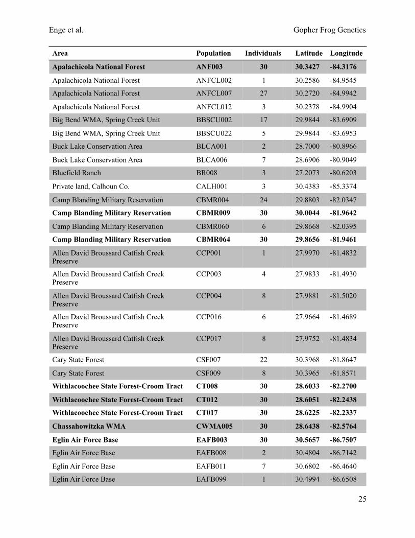
Table 2. Locality information for genotyped samples. Ponds with at least 30 samples are shown in bold.
" 24
Enge et al. Gopher Frog Genetics
Area Population Individuals Latitude Longitude
Apalachicola National Forest ANF003 30 30.3427 -84.3176
Apalachicola National Forest ANFCL002 1 30.2586 -84.9545
Apalachicola National Forest ANFCL007 27 30.2720 -84.9942
Apalachicola National Forest ANFCL012 3 30.2378 -84.9904
Big Bend WMA, Spring Creek Unit BBSCU002 17 29.9844 -83.6909
Big Bend WMA, Spring Creek Unit BBSCU022 5 29.9844 -83.6953
Buck Lake Conservation Area BLCA001 2 28.7000 -80.8966
Buck Lake Conservation Area BLCA006 7 28.6906 -80.9049
Bluefield Ranch BR008 3 27.2073 -80.6203
Private land, Calhoun Co. CALH001 3 30.4383 -85.3374
Camp Blanding Military Reservation CBMR004 24 29.8803 -82.0347
Camp Blanding Military Reservation CBMR009 30 30.0044 -81.9642
Camp Blanding Military Reservation CBMR060 6 29.8668 -82.0395
Camp Blanding Military Reservation CBMR064 30 29.8656 -81.9461
Allen David Broussard Catfish Creek Preserve
CCP001 1 27.9970 -81.4832
Allen David Broussard Catfish Creek Preserve
CCP003 4 27.9833 -81.4930
Allen David Broussard Catfish Creek Preserve
CCP004 8 27.9881 -81.5020
Allen David Broussard Catfish Creek Preserve
CCP016 6 27.9664 -81.4689
Allen David Broussard Catfish Creek Preserve
CCP017 8 27.9752 -81.4834
Cary State Forest CSF007 22 30.3968 -81.8647
Cary State Forest CSF009 8 30.3965 -81.8571
Withlacoochee State Forest-Croom Tract CT008 30 28.6033 -82.2700
Withlacoochee State Forest-Croom Tract CT012 30 28.6051 -82.2438
Withlacoochee State Forest-Croom Tract CT017 30 28.6225 -82.2337
Chassahowitzka WMA CWMA005 30 28.6438 -82.5764
Eglin Air Force Base EAFB003 30 30.5657 -86.7507
Eglin Air Force Base EAFB008 2 30.4804 -86.7142
Eglin Air Force Base EAFB011 7 30.6802 -86.4640
Eglin Air Force Base EAFB099 1 30.4994 -86.6508
" 25

Enge et al. Gopher Frog Genetics
Eglin Air Force Base EAFB101 30 30.6702 -86.4464
Etoniah Creek State Forest ECSF007 31 29.7867 -81.8759
Fort White Mitigation Park WEA FWMP008 31 29.8964 -82.7905
Green Swamp West GSW020 30 28.4271 -82.1276
Private land near Highlands Hammock HIGH001 30 27.4889 -81.5128
Halpata Tastanaki Preserve HTP027 30 29.0193 -82.3469
Jonathan Dickinson State Park JDSP005 5 26.9929 -80.1089
Jonathan Dickinson State Park JDSP008 8 27.0019 -80.1076
Jonathan Dickinson State Park JDSP011 13 26.9932 -80.1064
Jennings State Forest JSF002 1 30.0968 -81.9235
Jennings State Forest JSF003 15 30.1037 -81.9257
Jennings State Forest JSF004 12 30.1537 -81.9021
Jennings State Forest JSF010 22 30.1322 -81.8942
Jennings State Forest JSF012 30 30.1649 -81.9280
Jennings State Forest JSF031 35 30.1492 -81.8928
Jennings State Forest JSF039 6 30.1539 -81.9116
Little Big Econ State Forest LBESF011 23 28.6659 -81.1114
Longleaf Flatwoods Reserve LFR006 16 29.5639 -82.2004
Mosaic Fertilizer's Wellfield LMLW005 22 27.4656 -82.2008
Ocala National Forest ONFSL001 29 28.9767 -81.5637
Ocala National Forest ONFEGP002 14 29.3830 -81.7932
Ocala National Forest ONFEGP003 30 29.3788 -81.7941
Ocala National Forest ONFNSS008 30 29.4152 -81.7547
Ocala National Forest ONFRI006 32 29.4809 -81.8111
Ocala National Forest ONFSCL019 30 29.1664 -81.9046
Ocala National Forest ONFSL002 30 29.0558 -81.5612
Ocala National Forest ONFSSS010 30 29.3220 -81.7529
Rock Springs Run State Reserve RSRSR011 21 28.7720 -81.4532
Seminole State Forest SSF086 33 28.9911 -81.4472
St. Sebastian River Preserve State Park SSRP003 30 27.8278 -80.5868
St. Sebastian River Preserve State Park SSRP011 16 27.8408 -80.5226
St. Sebastian River Preserve State Park SSRP013 15 27.7948 -80.5128
St. Sebastian River Preserve State Park SSRP020 30 27.8374 -80.5386
" 26

Enge et al. Gopher Frog Genetics
Private land, Suwannee Co. SUWA002 7 30.0925 -82.8152
Triple N Ranch TNR003 19 28.1123 -81.0177
" 27

Enge et al. Gopher Frog Genetics
Table 3. Summary of genetic diversity estimates averaged over all loci and populations with >30 samples. Standard deviations were calculated by jackknifing over loci. 95% confidence intervals were calculated through bootstrapping over loci. Number of alleles (NA), effective number of alleles (Eff. NA), observed heterozygosity (HO), within population gene diversity (HS), overall gene diversity (HT), corrected overall gene diversity (H’T), and inbreeding coefficient (GIS).
Table 4. Genetic diversity estimates per locus and averaged over all loci for populations with at least 30 samples.
Statistic Mean StDev 95% CI
NA 23.700 1.571 (20.600, 26.400)
Eff. NA 4.688 0.170 (4.370, 5.004)
HO 0.790 0.014 (0.763, 0.815)
HS 0.798 0.008 (0.782, 0.813)
HT 0.889 0.007 (0.876, 0.902)
H’T 0.892 0.007 (0.879, 0.906)
GIS 0.009 0.012 (-0.012, 0.033)
Locus NA Eff NA HO HS HT H’T GIS
Raca7 28 4.182 0.733 0.797 0.898 0.902 0.080
Raca8 29 4.335 0.791 0.774 0.849 0.853 -0.023
Raca11 15 4.827 0.801 0.782 0.869 0.873 -0.024
Raca14 27 5.031 0.784 0.807 0.926 0.931 0.028
Raca25 17 5.374 0.800 0.816 0.908 0.912 0.019
Raca33 19 5.215 0.825 0.828 0.895 0.898 0.004
Raca37 26 5.257 0.807 0.823 0.908 0.912 0.020
Raca40 27 4.309 0.862 0.823 0.874 0.876 -0.046
Raca41 23 3.770 0.795 0.781 0.877 0.880 -0.017
Raca44 26 4.688 0.708 0.749 0.882 0.887 0.055
Overall 23.7 4.584 0.790 0.798 0.889 0.892 0.009
" 28

Enge et al. Gopher Frog Genetics
Table 5. Genetic diversity estimates for populations with at least 30 samples.
Table 6. Significance (P < 0.05) of heterozygosity-based tests for Hardy Weinberg equilibrium for populations with at least 30 samples. Values are 1-sided p-values of GIS (Nei 1987) per locus and population. Significant values are shown in bold.
Population NA Eff NA HO HS HT H’T GIS
EAFB003 8.200 4.704 0.720 0.771 0.771 --- 0.066
EAFB101 9.500 5.922 0.722 0.821 0.821 --- 0.120
ANF003 6.700 4.746 0.733 0.777 0.777 --- 0.057
FWMP008 7.300 4.320 0.730 0.767 0.767 --- 0.048
JSF012 8.800 4.589 0.735 0.773 0.773 --- 0.050
JSF031 5.700 4.215 0.746 0.742 0.742 --- -0.005
CBMR009 5.500 3.826 0.739 0.705 0.705 --- -0.048
CBMR064 9.600 5.872 0.769 0.834 0.834 --- 0.078
ECSF007 5.800 3.866 0.849 0.740 0.740 --- -0.149
ONFRI006 10.100 6.419 0.847 0.851 0.851 --- 0.005
ONFNSS008 11.100 6.597 0.838 0.851 0.851 --- 0.015
ONFEGP003 8.200 4.562 0.834 0.786 0.786 --- -0.060
ONFSSS010 9.800 6.058 0.799 0.837 0.837 --- 0.046
ONFSCL019 8.300 5.376 0.807 0.816 0.816 --- 0.010
HTP027 12.100 7.448 0.873 0.875 0.875 --- 0.002
ONFSL002 12.200 7.744 0.843 0.882 0.882 --- 0.044
SSF086 7.900 4.934 0.869 0.800 0.800 --- -0.086
CWMA005 8.700 4.707 0.769 0.793 0.793 --- 0.030
CT008 11.100 7.123 0.870 0.869 0.869 --- -0.001
CT012 9.700 6.268 0.821 0.847 0.847 --- 0.031
CT017 11.000 6.886 0.837 0.857 0.857 --- 0.023
GSW020 10.300 6.265 0.857 0.845 0.845 --- -0.013
SSRP020 4.300 2.906 0.734 0.638 0.638 --- -0.149
SSRP003 7.600 4.365 0.742 0.759 0.759 --- 0.022
HIGH001 4.800 3.602 0.680 0.710 0.710 --- 0.042
" 29

Enge et al. Gopher Frog Genetics
Population Raca7 Raca8 Raca11 Raca14 Raca25 Raca33 Raca37 Raca40 Raca41 Raca44Multi-locus
EAFB003 0.123 0.274 0.065 0.157 0.164 0.569 0.005 0.188 0.477 0.001 0.005
EAFB101 0.541 0.143 0.575 0.190 0.007 0.057 0.006 0.002 0.522 0.019 0.001
ANF003 0.525 0.051 0.238 0.425 0.078 0.101 0.431 0.070 0.045 0.001 0.018
FWMP008 0.109 0.084 0.111 0.336 0.001 0.276 0.013 0.024 0.289 0.002 0.006
JSF012 0.001 0.940 0.964 0.152 0.473 0.113 0.429 0.006 0.554 0.160 0.001
JSF031 0.007 0.043 0.353 0.001 0.742 0.191 0.505 0.001 0.067 0.001 0.990
CBMR009 0.003 0.583 0.026 0.035 0.345 0.232 0.083 0.001 0.296 0.125 0.077
CBMR064 0.001 0.517 0.009 0.001 0.003 0.141 0.219 0.233 0.066 0.582 0.001
ECSF007 0.448 0.357 0.091 0.001 0.403 0.459 0.252 0.001 0.169 0.001 0.001
ONFRI006 0.155 0.392 0.026 0.637 0.040 0.106 0.513 0.311 0.531 0.056 0.419
ONFNSS008 0.216 0.285 0.016 0.243 0.046 0.017 0.551 0.246 0.071 0.064 0.212
ONFEGP003 0.077 0.035 0.009 0.496 0.166 0.093 0.030 0.002 0.045 0.496 0.020
ONFSSS010 0.129 0.215 0.074 0.344 0.002 0.040 0.501 0.002 0.184 0.001 0.023
ONFSCL019 0.113 0.003 0.751 0.795 0.033 0.071 0.547 0.270 0.340 0.001 0.001
HTP027 0.466 0.339 0.531 0.490 0.167 0.448 0.038 0.144 0.008 0.078 0.388
ONFSL002 0.552 0.002 0.458 0.486 0.458 0.303 0.326 0.006 0.467 0.610 0.013
SSF086 0.015 0.023 0.404 0.029 0.011 0.445 0.022 0.506 0.045 0.171 0.001
CWMA005 0.001 0.049 0.001 0.284 0.033 0.149 0.014 0.001 0.254 0.174 0.004
CT008 0.461 0.371 0.184 0.004 0.283 0.590 0.498 0.175 0.017 0.231 0.523
CT012 0.522 0.260 0.610 0.002 0.105 0.442 0.592 0.624 0.228 0.403 0.052
CT017 0.296 0.111 0.177 0.032 0.527 0.602 0.262 0.472 0.107 0.347 0.166
GSW020 0.331 0.548 0.100 0.328 0.202 0.485 0.073 0.562 0.383 0.004 0.295
SSRP020 0.246 0.054 0.077 0.233 0.468 0.001 0.007 0.544 0.247 0.045 0.001
SSRP003 0.082 0.195 0.482 0.382 0.470 0.361 0.014 0.190 0.070 0.001 0.001
HIGH001 0.167 0.001 0.003 0.002 0.048 0.405 0.048 0.213 0.008 0.211 0.057
" 30
Enge et al. Gopher Frog Genetics
Table 7. Population differentiation statistics per locus and averaged over all loci for populations with at least 30 samples: F-statistic analogs for microsatellites based on allele size (RhoIS RhoST RhoIT [Rousset 1996]; 1 locus estimates following standard ANOVA analogous to Weir and Cockerham [1984]; see Michalakis and Excoffie [1996] for formulas); fixation index (FST) based on allele identity (Cockerham 1973, Weir and Cockerham 1984); coefficient of gene differentiation, both in its original form (GST; Nei 1973) and as standardized by levels of genetic variation (G’ST [Hedrick 2005]; G’’ST [Meirmans and Hedrick 2011]); and Jost’s D (DEST; Jost 2008).
Locus RhoIS RhoST RhoIT FST GST G’ST G’’ST DEST
Raca7 0.151 0.408 0.498 0.118 0.113 0.574 0.576 0.520
Raca8 -0.116 0.160 0.063 0.093 0.089 0.406 0.408 0.348
Raca11 -0.072 0.173 0.113 0.103 0.100 0.476 0.478 0.417
Raca14 0.106 0.116 0.210 0.134 0.129 0.691 0.693 0.646
Raca25 -0.008 0.144 0.138 0.106 0.102 0.570 0.572 0.522
Raca33 -0.037 0.118 0.085 0.079 0.075 0.452 0.453 0.407
Raca37 0.049 0.141 0.182 0.098 0.094 0.548 0.550 0.501
Raca40 0.373 0.077 0.421 0.060 0.058 0.340 0.342 0.299
Raca41 0.008 0.194 0.201 0.113 0.109 0.514 0.516 0.454
Raca44 0.014 0.081 0.094 0.147 0.150 0.617 0.620 0.550
Overall 0.075 0.219 0.278 0.105 0.102 0.522 0.524 0.468
" 31
Enge et al. Gopher Frog Genetics
Table 8. Private alleles by locus and population.
Table 9. Analysis of molecular variance (AMOVA) using an infinite allele model (reported statistics are equivalent to Rho). Significance was tested using 10,000 permutations. Standard deviations of F-statistics were obtained through jackknifing over loci. 95% confidence intervals of F-statistics were obtained through bootstrapping over loci.
Locus Population Allele Locus Population Allele Locus Population Allele
Raca7 CBMR009 334 Raca25 CWMA005 364 Raca40 SUWA002 286
Raca7 JSF004 346 Raca25 LBESF011 258 Raca40 SUWA002 346
Raca7 ONFLD001 266 Raca25 ONFLD001 264 Raca41 CWMA005 336
Raca7 ONFEGP002 294 Raca33 BLCA001 277 Raca41 LMLW005 292
Raca7 ONFLD001 430 Raca33 JSF003 215 Raca44 ANF003 333
Raca7 SSRP003 402 Raca33 JSF004 201 Raca44 CBMR004 357
Raca8 HTP027 384 Raca37 CCP003 209 Raca44 CT008 363
Raca8 LBESF011 308 Raca37 CT017 253 Raca44 HTP027 391
Raca8 SUWA002 388 Raca37 FWMP008 157 Raca44 HTP027 405
Raca14 CBMR004 308 Raca37 ONFEGP002 173 Raca44 LBESF011 395
Raca14 EAFB008 310 Raca37 RSRSR011 245 Raca44 LFR006 341
Raca14 ONFEGP002 304 Raca40 CWMA005 382 Raca44 ONFEGP002 377
Raca14 ONFSCL019 212 Raca40 EAFB008 318 Raca44 RSRSR011 389
Raca14 ONFSCL019 222 Raca40 LBESF011 322
Raca14 SUWA002 290 Raca40 SUWA002 286
Variance component % total variance F-stat F-value P-value
Within population 0.816 -- -- --
Among population 0.184 RhoST 0.184 0.000
" 32

Enge et al. Gopher Frog Genetics
Table 10. Models of demographic history specified for the panhandle/peninsula divergence tested in Migrate. The best model (shown in bold) has log Bayes factor (LBF) of 0.0 because the best model is used as a reference in Migrate.
Model Log(mL) LBFModel
probability
1: Split with immigration to the east -62432.90 0.00 1.0000
2: Split without immigration -63342.03 -909.13 0.0000
3: Immigration to the east only -68137.96 -5705.06 0.0000
4: Immigration to the east and west -68665.67 -6232.77 0.0000
5: Immigration to the west only -68752.47 -6319.57 0.0000
6: Split with immigration to the west only -77835.94 -15403.04 0.0000
7: Panmixia -120335.72 -57902.82 0.0000
" 33

Enge et al. Gopher Frog Genetics
Table 11. Matrix of inferred (posterior mean) migration rates and the standard deviation of the marginal posterior distribution for each estimate (in parentheses) for a group of ponds in the Jennings State Forest/Camp Blanding Military Reservation region. m[i][j] is the per-generation fraction of individuals in population i that are migrants from population j. Estimates were generated using BayesAss.
Table 12. Matrix of inferred (posterior mean) migration rates and the standard deviation of the marginal posterior distribution for each estimate (in parentheses) for a group of ponds in the Ocala National Forest region. m[i][j] is the per-generation fraction of individuals in population i that are migrants from population j. Estimates were generated using BayesAss.
JSF012 JSF031 JSF010 CBMR009 CBMR004 CBMR064 ECSF007
JSF012 0.9207 (0.0270)
0.0193 (0.0155)
0.0170 (0.0141)
0.0095 (0.0092)
0.0118 (0.0112)
0.0121 (0.0121)
0.0095 (0.0093)
JSF031 0.0118 (0.0102)
0.9481 (0.0189)
0.0082 (0.0080)
0.0080 (0.0078)
0.0080 (0.0078)
0.0080 (0.0079)
0.0079 (0.0078)
JSF010 0.2224 (0.0399)
0.0144 (0.0139)
0.6870 (0.0217)
0.0177 (0.0158)
0.0222 (0.0199)
0.0168 (0.0161)
0.0196 (0.0158)
CBMR009 0.0093 (0.0090)
0.0090 (0.0088)
0.0091 (0.0087)
0.9453 (0.0200)
0.0092 (0.0089)
0.0091 (0.0088)
0.0090 (0.0088)
CBMR004 0.0210 (0.0175)
0.0123 (0.0117)
0.0125 (0.0121)
0.0123 (0.0117)
0.8833 (0.0447)
0.0289 (0.0375)
0.0297 (0.0227)
CBMR064 0.0197 (0.0171)
0.0091 (0.0088)
0.0100 (0.0098)
0.0126 (0.0120)
0.1803 (0.0804)
0.7590 (0.0809)
0.0093 (0.0091)
ECSF007 0.0093 (0.0089)
0.0090 (0.0088)
0.0090 (0.0088)
0.0094 (0.0091)
0.0089 (0.0088)
0.0088 (0.0085)
0.9456 (0.0200)
ONFRI006 ONFNSS008 ONFEGP003 ONFSSS010 ONFSCL019 ONFSL002 SSF086 ONFLD001
ONFRI006 0.8034 (0.0405)
0.0108 (0.0110)
0.0430 (0.0292)
0.0092 (0.0090)
0.0119 (0.0115)
0.0782 (0.0358)
0.0329 (0.0269)
0.0106 (0.0103)
ONFNSS008 0.0222 (0.0214)
0.6869 (0.0142)
0.1457 (0.0364)
0.0099 (0.0098)
0.0125 (0.0119)
0.0765 (0.0352)
0.0277 (0.0188)
0.0186 (0.0171)
ONFEGP003 0.0110 (0.0108)
0.0091 (0.0088)
0.9101 (0.0280)
0.0090 (0.0087)
0.0102 (0.0101)
0.0103 (0.0101)
0.0305 (0.0201)
0.0099 (0.0097)
ONFSSS010 0.0392 (0.0328)
0.0096 (0.0094)
0.0110 (0.0106)
0.7675 (0.0257)
0.0091 (0.0088)
0.1431 (0.0389)
0.0110 (0.0106)
0.0095 (0.0092)
ONFSCL019 0.0178 (0.0166)
0.0099 (0.0097)
0.0190 (0.0151)
0.0228 (0.0207)
0.8797 (0.0317)
0.0259 (0.0202)
0.0132 (0.0130)
0.0117 (0.0112)
" 34

Enge et al. Gopher Frog Genetics
ONFSL002 0.0589 (0.0352)
0.0109 (0.0105)
0.0401 (0.0270)
0.0132 (0.0131)
0.0174 (0.0144)
0.6902 (0.0267)
0.0131 (0.0126)
0.1562 (0.0416)
SSF086 0.0163 (0.0156)
0.0129 (0.0121)
0.0083 (0.0083)
0.0091 (0.0089)
0.0097 (0.0100)
0.0139 (0.0132)
0.9194 (0.0266)
0.0104 (0.0102)
ONFLD001 0.0163 (0.0148)
0.0097 (0.0093)
0.0199 (0.0169)
0.0100 (0.0096)
0.0118 (0.0113)
0.1277 (0.0566)
0.0110 (0.0105)
0.7936 (0.0534)
" 35

Enge et al. Gopher Frog Genetics
Figure 1. Locations of potentially extant gopher frog populations in relation to factors that may isolate populations (urban areas, silviculture, agriculture, mining, interstates, and major rivers).
" 36

Enge et al. Gopher Frog Genetics
"
Figure 2. Locations of areas of occupancy for the collection of genetic samples. These areas represent potentially isolated populations.
" 37

Enge et al. Gopher Frog Genetics
Figure 3. Locations of all 64 sampled ponds (left map) and locations of ponds with at least 30 sampled individuals (right map).
Figure 4. A)
Populations used in Migrate analyses. Orange circles represent populations combined into a panhandle “population.” Blue circles represent peninsular populations that were combined. Polygons represent county boundaries. B) Seven models tested in Migrate analysis. Model 1: split with immigration to the east; 2: split without immigration; 3: immigration to the east only; 4: immigration to the east and west; 5: immigration to the west only; 6: split with immigration to the west only; 7: panmixia.
" 38
B
A
Enge et al. Gopher Frog Genetics
"
Figure 5. Ponds in the Ocala National Forest region (left map) and Jennings State Forest/Camp Blanding Military Reservation region (right map) used to estimate migration in the software BayesAss.
" 39

Enge et al. Gopher Frog Genetics
Figure 6. Number of alleles per locus (left panel) and rarefied allelic counts per locus for populations with at least 30 individuals (right panel).
Figure 7. Scatterplots of diversity partitioning estimators vs. locus polymorphism. Red lines are best-fit lines, and r-values are Pearson product moment correlation coefficients. A significant correlation does not exist between locus polymorphism and diversity partitioning statistics (see Keenan et al. 2013).
" 40
Enge et al. Gopher Frog Genetics
!
Figure 8. Mean within-population pairwise relatedness r for each population estimated using Queller and Goodnight's (1989) estimator. The coefficient of relatedness ranges from -1 (no shared alleles) to 1 (identical twins or clones). Negative values indicate pairwise relatedness was less than expected between 2 randomly chosen individuals. In an outbred diploid population, expected relatedness between full-sibling groups is r = 0.5 (r = 0.25 for half-sibling groups). Individuals chosen at random should have r = 0. Upper and lower error bars bound the 95% confidence interval around the mean as determined by 100 bootstrap replicates. Upper and lower confidence limits bound the 95% confidence interval about the null hypothesis of ‘no difference’ across populations as determined by 99 permutations.
" 41

Enge et al. Gopher Frog Genetics
" 42

Enge et al. Gopher Frog Genetics
Figure 9. Results from Structure analysis of the entire dataset assuming admixture with correlated allele frequencies among populations and using location information as a prior. (A) mean log probability of the data is highest for K = 17; (B) the rate of change in the log probability of the data (ΔK) is greatest from 1 to 2 clusters, and nearly as great from 2 to 3 clusters; (C, E) at K = 2, panhandle and peninsular populations form separate clusters; (D, F) at K = 3, St. Sebastian River Preserve populations form a third cluster.
" 43
A B
C

Enge et al. Gopher Frog Genetics
" 44
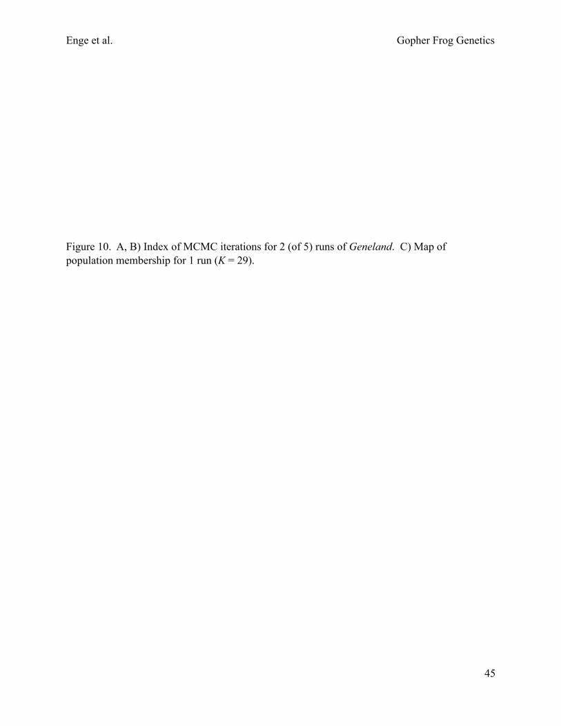
Enge et al. Gopher Frog Genetics
Figure 10. A, B) Index of MCMC iterations for 2 (of 5) runs of Geneland. C) Map of population membership for 1 run (K = 29).
" 45

Enge et al. Gopher Frog Genetics
"
Figure 11. A) Seven ponds in the Jennings State Forest/Camp Blanding Military Reservation region used to estimate migration rates in BayesAss. B) Circle plot showing migration among populations, where line width is proportional to migration rate estimate (i.e., wider lines indicate relatively greater migration rates). Estimates are shown in Table 11, and very small migration rates are not shown for clarity.
" 46
A B
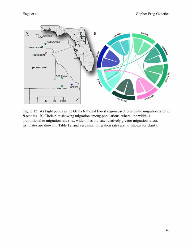
Enge et al. Gopher Frog Genetics
Figure 12. A) Eight ponds in the Ocala National Forest region used to estimate migration rates in BayesAss. B) Circle plot showing migration among populations, where line width is proportional to migration rate (i.e., wider lines indicate relatively greater migration rates). Estimates are shown in Table 12, and very small migration rates are not shown for clarity.
" 47
A B