Genetic Algorithm Project Report

Brian Satzinger

November 2, 2009

Abstract

A genetic algorithm is used to optimize the allocation of video processing plug-ins to nodes

in a distributed video processing network. GPU performance in each node as well as network

congestion on the network is modeled in order to find an allocation which is sufficient to process

video at 30 frames per second, which is the upper limit of the cameras used in the network.

Contents

1 Introduction 2

1.1 Description of Video Processing Network . . . . . . . . . . . . . . . . . . . . . . . . . . 2

1.2 Description of Genetic Algorithm . . . . . . . . . . . . . . . . . . . . . . . . . . . . . . 3

1.2.1 Chromosome Representation . . . . . . . . . . . . . . . . . . . . . . . . . . . . 3

1.2.2 Selection Operator . . . . . . . . . . . . . . . . . . . . . . . . . . . . . . . . . . 4

1.2.3 Crossover Operator . . . . . . . . . . . . . . . . . . . . . . . . . . . . . . . . . . 4

1.2.4 Mutation Operator . . . . . . . . . . . . . . . . . . . . . . . . . . . . . . . . . . 5

1.2.5 Other Parameters . . . . . . . . . . . . . . . . . . . . . . . . . . . . . . . . . . 6

2 Development of the Fitness Function 6

2.1 Modeling Plug-in Performance . . . . . . . . . . . . . . . . . . . . . . . . . . . . . . . 6

2.2 Modeling Network Performance . . . . . . . . . . . . . . . . . . . . . . . . . . . . . . . 8

2.3 Determining GPU Fitness . . . . . . . . . . . . . . . . . . . . . . . . . . . . . . . . . . 12

2.4 Determining Network Fitness . . . . . . . . . . . . . . . . . . . . . . . . . . . . . . . . 12

2.5 Determining Overall Fitness . . . . . . . . . . . . . . . . . . . . . . . . . . . . . . . . . 14

2.6 Observations About The Fitness Function . . . . . . . . . . . . . . . . . . . . . . . . . 15

1

3 Discussion of Implementation 15

3.1 Chromosome.java . . . . . . . . . . . . . . . . . . . . . . . . . . . . . . . . . . . . . . . 15

3.2 Population.java . . . . . . . . . . . . . . . . . . . . . . . . . . . . . . . . . . . . . . . . 16

3.3 Plugin.java . . . . . . . . . . . . . . . . . . . . . . . . . . . . . . . . . . . . . . . . . . 16

3.4 Fitness.java . . . . . . . . . . . . . . . . . . . . . . . . . . . . . . . . . . . . . . . . . . 16

3.5 Constants.java . . . . . . . . . . . . . . . . . . . . . . . . . . . . . . . . . . . . . . . . 16

3.6 Main.java . . . . . . . . . . . . . . . . . . . . . . . . . . . . . . . . . . . . . . . . . . . 17

4 Experimental Results and Analysis 17

4.1 Mutation Method . . . . . . . . . . . . . . . . . . . . . . . . . . . . . . . . . . . . . . . 17

4.2 Mutation Rate . . . . . . . . . . . . . . . . . . . . . . . . . . . . . . . . . . . . . . . . 19

4.3 Crossover Method . . . . . . . . . . . . . . . . . . . . . . . . . . . . . . . . . . . . . . 21

4.4 Selection Method . . . . . . . . . . . . . . . . . . . . . . . . . . . . . . . . . . . . . . . 22

5 Conclusion 24

1 Introduction

1.1 Description of Video Processing Network

This lab report concerns the development of a genetic algorithm for plug-in load balancing on Dr.

DeSouza’s ViGIR image processing network. The network consists of a number of nodes, each of which

is capable of instantiating a number of image processing plug-ins, which perform some manipulation

of the image (such as edge detection). These plug-ins can be connected in sequences to perform more

complicated operations on the images.

The plug-ins process video streams, which can provide up to 30 images per second from a number

of cameras built into the environment. These video streams can flow between two plug-ins on the

same node, or between two plug-ins on different nodes over a gigabit ethernet network.

The interconnection of the plug-ins is given as part of the input to the genetic algorithm. The

genetic algorithm determines a mapping of plug-ins to nodes in order to give optimal network per-

formance. The challenge in finding a good mapping is that reduced performance can come from two

sources. First, it is possible for too many plug-ins to be instantiated on a single node, reducing frame

rate at which the GPU can execute the plug-ins. Second, it is possible for too many video streams to

2

be transmitted across the network, which can reduce the frame rate in the video stream. The solution

for the first problem is to distribute plug-ins across as many nodes as possible, while the solution

to the second problem is to concentrate plug-ins across as few nodes as possible. These conflicting

objectives make optimization a challenging problem. In general, the genetic algorithm must strike a

balance between these two by intelligently grouping related plug-ins on the same nodes.

1.2 Description of Genetic Algorithm

The solution created for this project is a genetic algorithm. Candidate solutions are represented as a

chromosome, which encodes the location of each plug-in as an integer. Chromosomes are evaluated

using a fitness function which uses a model of the network’s performance to predict the frame rate

achievable with the network configuration encoded in the chromosome. Selection can use several

different selection algorithms, such as proportional selection, and elitism. One point, two point, and

random crossover algorithms are evaluated to determine their suitability to this problem domain.

The mutation operator randomly increments and decrements integers within the chromosomes. An

additional mutation operator is also discussed which swaps two random genes within the chromosome.

Other parameters are also discussed, including the population size and the definition of convergence.

A description of the algorithm used is shown below in Algorithm 1.

Algorithm 1 Genetic Algorithm• Create a random initial population

• Do Until Convergence

– Calculate the fitness of all individuals in the population

– Select half of the population using the selection operator, remove the remaining individualsfrom the population

– Perform crossover on the selected individuals and add their children to the population

– Randomly perform mutation on individuals in the population

• After convergence, use the most fit individual as the solution

1.2.1 Chromosome Representation

In this problem, the purpose of the genetic algorithm is to map plug-ins into a fixed number of nodes.

This mapping can be acheived by associating each plug-in with a single integer lp which identifies the

location of the plug-in. Therefore, for a problem with N nodes and P plug-ins, the chromosome will

3

take the form of a vector of length P whose elements are integers restricted to the range [0, N − 1]. A

single integer (gene) within the chromosome is the smallest element that will be operated on directly

by crossover and mutation operations. Bit-level manipulations are not used.

Chromosome = [l1, ... lp ... , lP ]

Where lp ∈ N and 0 ≤ lp ≤ N − 1

1.2.2 Selection Operator

The selection operator is used to select half of the population for crossover and mutation based on

the fitness of individuals within the population. The fitness function is somewhat complex, and is

described in Section 2. In general, the fitness of a chromosome is a real number between 0 and 30

which represents the predicted performance of the network configuration (in frames per second) based

on the algorithm described in Section 2.

Proportional selection can be used in the genetic algorithm. In this case, the fitness of all of the

individuals in the population is calculated, and individuals are selected for crossover and mutation

in a probabilistic way. The probability of an individual being selected is calculated using Equation

1. pi is the probability of selecting individual i, and fi is the fitness of individual i. For an original

population consisting of N individuals, N2 individuals are selected by repeatedly selecting individuals

at random from the population. Note that this allows individuals (especially those of higher fitness)

to be selected multiple times.

pi=

fiPNj=1 fj

(1)

Another selection operator can be used, in which the fittest N2 individuals are selected for crossover.

This elitist method is simpler to implement compared to proportional selection. In the results section,

the performance of these two operators will be compared.

1.2.3 Crossover Operator

Three different crossover operations can be used. One-point, two-point, and uniform crossover can be

applied to two parent chromosomes to generate two child chromosomes which contain a redistribution

of the genes in the parents.

4

In one-point crossover, a location is randomly selected within the chromosome, known as the

crossover point. A crossover mask is generated, which consists of a bit-string of the same length as

the chromosome. For all bits before the crossover point, a zero is stored in the bit-string, and for all

other locations, a one is stored in the bit-string. Child 1 is generated by copying a gene from parent 1

for each location in the mask which is a zero, and from parent 2 for each location in the mask which

is a one. Child 2 is generated by copying a gene from parent 2 for each location in the mask which is

a zero, and from parent 1 for each location in the mask which is a one.

For two-point crossover, two crossover points are selected at random. They are used to generate

a crossover mask which is zero until the lowest crossover point is reached, then becomes one until the

other crossover point is reached, at which point it is zero until the end of the string. Children are

generated from the crossover mask as described above.

In uniform crossover, the crossover mask is generated randomly, with an equal probability of zeros

and ones. The children are then generated using this crossover mask.

These three crossover operations represent various levels of “mixing” of the genes in the parent

chromosomes. Single point crossover maintains the largest sequential groups of genes from the parent

chromosomes, with two-point crossover maintaining smaller groups, and uniform crossover not nec-

essarily maintaining any sequential groups of genes. In this problem domain, the relative location

of plug-ins is significant, so these three crossover operators may give different results. This will be

explored in the results section.

1.2.4 Mutation Operator

The genes in the chromosome take the form of integers. The mutation operator randomly selects genes

within the population with probability pm and either adds or subtracts one (with equal probability)

from the value. If this results in an invalid number (less than 0 or equal to the number of plug-ins),

the operator then normalizes the result by wrapping the result around. For example, if a gene is

initially equal to 0, and the mutation operator subtracts 1 from it, this will result in -1. This value is

wrapped around to the highest valid node number, which is equal to the number of nodes - 1.

An alternative mutation operator can also be used. This mutation operator selects chromosomes

with probability pm_swap. Two genes are randomly selected from within this chromosome and their

values are exchanged. This operator has the effect of switching the location of two plug-ins. In this

problem domain, switching plug-in locations like this is often desired in order to minimize the number

5

of streams which traverse the network. See Figure 4 for an example of a network configuration which

would be improved by swapping several plug-ins.

1.2.5 Other Parameters

The population size is a parameter which must be determined. In general, a larger population size

allows for greater exploration of the search space at the cost of increasing the time it takes to process a

single generation. The optimum population size might depend on the complexity (number of plug-ins)

of the plug-in network which the program is optimizing.

The definition of convergence is another parameter that should be adjusted. In this case, the

best performance that can possibly be achieved is 30 frames per second (because of limitations in

the cameras). Assuming that the fitness function reflects actual performance, the algorithm should

be stopped once an individual in the population achieves a fitness of 30, since further searching is

unnecessary. For difficult problems with a large number of plug-ins, it might not be possible to achieve

30 frames per second, so the program should allow this target value to be reduced. Alternatively, the

program could also be restricted to only generate a finite number of generations and pick the best

solution based on the performance up to that point.

2 Development of the Fitness Function

The fitness function will be based on the GPU and network performance models described in sub-

sections 2.1 and 2.2. Based on the mapping of plug-ins to nodes described in the chromosome, the

fitness function will estimate the frame rate achievable on each node’s GPU and on each link in the

network. The value returned by the fitness function will be the smallest of these values.

2.1 Modeling Plug-in Performance

In the image processing network, each node is capable of instantiating a number of different GPU

plug-ins in order to perform some manipulation of image data. Each of these plug-ins consumes

GPU resources, and it is important for load balancing that this resource consumption be accurately

modeled. For each plug-in, the node was configured to run N instances of the plug-in, where N was

varied between 1 and 50.

As the number of plug-in instances increased, the GPU eventually became over utilized, and the

6

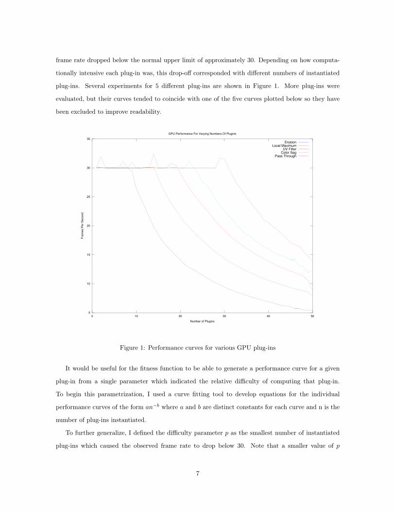
frame rate dropped below the normal upper limit of approximately 30. Depending on how computa-

tionally intensive each plug-in was, this drop-off corresponded with different numbers of instantiated

plug-ins. Several experiments for 5 different plug-ins are shown in Figure 1. More plug-ins were

evaluated, but their curves tended to coincide with one of the five curves plotted below so they have

been excluded to improve readability.

5

10

15

20

25

30

35

0 10 20 30 40 50

Fra

me

s P

er

Se

co

nd

Number of Plugins

GPU Performance For Varying Numbers Of Plugins

ErosionLocal Maximum

UV FilterColor Seg

Pass Through

Figure 1: Performance curves for various GPU plug-ins

It would be useful for the fitness function to be able to generate a performance curve for a given

plug-in from a single parameter which indicated the relative difficulty of computing that plug-in.

To begin this parametrization, I used a curve fitting tool to develop equations for the individual

performance curves of the form an−b where a and b are distinct constants for each curve and n is the

number of plug-ins instantiated.

To further generalize, I defined the difficulty parameter p as the smallest number of instantiated

plug-ins which caused the observed frame rate to drop below 30. Note that a smaller value of p

7

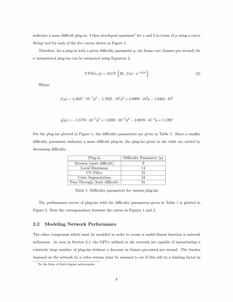
indicates a more difficult plug-in. I then developed equations1 for a and b in terms of p using a curve

fitting tool for each of the five curves shown in Figure 1.

Therefore, for a plug-in with a given difficulty parameter p, the frame rate (frames per second) for

n instantiated plug-ins can be estimated using Equation 2.

FPS(n, p) = MIN{

30, f(p) · n−g(p)}

(2)

Where

f(p) = 4.4027 · 10−1p3 − 1.7625 · 101p2 + 2.6909 · 102p− 1.0404 · 103

g(p) = −1.5778 · 10−5p3 + 1.6282 · 10−3p2 − 2.6919 · 10−2p + 1.1297

For the plug-ins plotted in Figure 1, the difficulty parameters are given in Table 1. Since a smaller

difficulty parameter indicates a more difficult plug-in, the plug-ins given in the table are sorted by

decreasing difficulty.

Plug-in Difficulty Parameter (p)Erosion (most difficult) 9

Local Maximum 14UV Filter 21

Color Segmentation 24Pass Through (least difficult) 31

Table 1: Difficulty parameters for various plug-ins

The performance curves of plug-ins with the difficulty parameters given in Table 1 is plotted in

Figure 2. Note the correspondence between the curves in Figures 1 and 2.

2.2 Modeling Network Performance

The other component which must be modeled in order to create a useful fitness function is network

utilization. As seen in Section 2.1, the GPUs utilized in the network are capable of instantiating a

relatively large number of plug-ins without a decrease in frames processed per second. The burden

imposed on the network by a video stream must be assessed to see if this will be a limiting factor in1In the form of third degree polynomials

8

5

10

15

20

25

30

35

0 10 20 30 40 50

Estim

ate

d F

ram

es P

er

Se

co

nd

Number of Plugins

Estimated Performance For Varying Numbers Of Plugins By Difficulty Parameter

p=9p=14p=21p=24p=31

Figure 2: Frames per second predicted using Equation 2 as a model of plug-in performance.

9

overall performance.

The bandwidth consumed by a single video stream was estimated to be approximately 30 megabytes

per second by monitoring total network traffic over a five minute interval and calculating the average

rate. In fact, the video is transmitted over the network at a resolution of 640 by 480, at 30 frames per

second, and 3 bytes of data per pixel, which corresponds to 27.6 megabytes per second, or 221 megabits

per second2, as shown in Equation 3. The additional data which was observed in the informal test

can be attributed to network overhead, network traffic from other programs, and timing inaccuracy.

640 · 480pixels

frame· 30

frames

second· 3 bytes

pixel= 27648000

bytes

second= 27.6

megabytes

second= 221

megabits

second(3)

The network utilized in the lab consists of switched gigabit ethernet. Theoretically, each node

would be able to receive and transmit one gigabit per second simultaneously, however in practice

ethernet switches cannot support that amount of throughput on all of their ports at once. As the

switch becomes congested, it will drop packets, leading to reduced throughput, and eventually a

reduction in the observed frame rate of the video signal.

Unfortunately, it was not possible to test the switch by generating traffic until the switch became

congested without disrupting other users of the network. Therefore, the performance of the network

under heavy loads can only be estimated. For purposes of modeling the behavior of the network,

assume that the switch is capable of switching packets without dropping them even if all of its ports

are saturated with traffic. In this case, the source of congestion will come from multiple video streams

attempting to share the single gigabit link between each node and the central switch. Note that this

is an optimistic model and that actual performance will be somewhat lower than this.

For n video streams sharing a 1 gigabit link, the bandwidth available to each link is 1 gigabitsecond

n . As

long as this value remains above 221 megabits per second, each of the streams will be able to maintain

30 frames per second. However, if n grows large enough (greater than 4), it will not be possible for

each stream to maintain 30 frames per second. In this case, assuming that the link is shared evenly

between the n streams, the frames per second transmitted on each link will be reduced, as shown

below.

bandwidth_per_stream(n) =1000 megabits

second· 1n

2The video stream is not compressed before sending it over the network

10

frame_rate_per_stream(n) =1000 megabits

second · 1n

221 megabitssecond

· 30frames

second=

1000n

221· 30 =

30000221 · n

actual_frame_rate(n) = min{30,30000221 · n

} (4)

A plot of actual_frame_rate(n) is shown in Figure 3. Note that the network begins to constrain

video performance after more than four simultaneous streams share a single network link. Compared

with Figure 2, this shows that the network is a greater performance constraint than GPU performance.

This suggests that the genetic algorithm will generate solutions which minimize the number of video

streams entering and leaving each node until n ≤ 4.

0

5

10

15

20

25

30

35

0 2 4 6 8 10 12 14

Fra

me

s p

er

se

co

nd

pe

r str

ea

m

Number of video streams

Network Congestion For Different Numbers Of Simultaneous Steams

Figure 3: Estimate of video stream performance with multiple video streams sharing the same gigabitethernet link

11

2.3 Determining GPU Fitness

The difficulty parameter p is all that will be specified for each plug-in. For the set of plug-ins mapped

to a given node by a chromosome, a difficulty vector can be written, as shown in Equation 5.

P = [p1 ... pn] (5)

The difficulty parameters for all of the plug-ins can be combined to give an equivalent difficulty

score using Equation 6. This expression returns a difficulty parameter which corresponds to some

plug-in which, when instantiated n times, will be equivalent to instantiating n plug-ins with the

various difficulty parameters given in P. The reason for combining difficulty parameters in this way

is based in the definition of p , which is defined as the smallest number of instances of a given plug-in

which causes the GPU to produce fewer than 30 frames per second. Based on this, 1p corresponds to

the fraction of the GPU’s resources used by a single plug-in at 30 frames per second. Summing 1pn

gives an estimate for the total GPU utilization created by the difficulty vector P. Taking one over

the sum gives the difficulty parameter for a single plug-in which is equivalent to all of the plug-ins

in P. Multiplying by N creates a difficulty parameter which corresponds to a plug-in which must be

instantiated n times to be as difficult as P. This could be interpreted as giving an “average” difficulty

of the plug-ins in P, and allows the model given in Equation 2 to be used to estimate the frame rate.

Peq =N∑N

n=11

pn

(6)

For each node, the video frame rate is estimated as described above. The overall GPU fitness score

is determined to be the smallest frame rate observed on any node.

2.4 Determining Network Fitness

The number of video streams produced by a network configuration must be determined algorithmically.

This can be determined from the information contained within two tables. The plug-in table specifies

the interconnections between plug-ins, while the chromosome specifies the node on which each plug-

in will be instantiated. The combination of the plug-in table and the chromosome can be used to

determine how many video streams will traverse each link in the network. Equation 4 can then be

used to estimate the performance (in frames per second) of the video.

For example, Figure 4 shows an example network configuration which illustrates how network

12

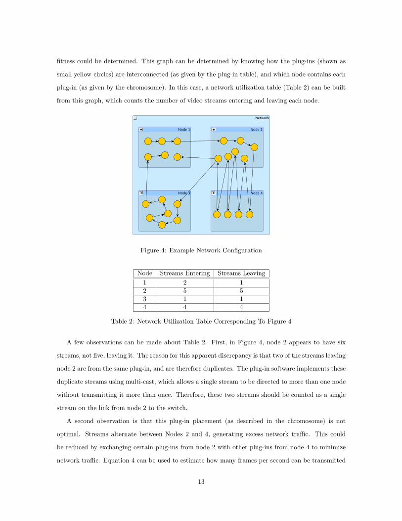
fitness could be determined. This graph can be determined by knowing how the plug-ins (shown as

small yellow circles) are interconnected (as given by the plug-in table), and which node contains each

plug-in (as given by the chromosome). In this case, a network utilization table (Table 2) can be built

from this graph, which counts the number of video streams entering and leaving each node.

Figure 4: Example Network Configuration

Node Streams Entering Streams Leaving1 2 12 5 53 1 14 4 4

Table 2: Network Utilization Table Corresponding To Figure 4

A few observations can be made about Table 2. First, in Figure 4, node 2 appears to have six

streams, not five, leaving it. The reason for this apparent discrepancy is that two of the streams leaving

node 2 are from the same plug-in, and are therefore duplicates. The plug-in software implements these

duplicate streams using multi-cast, which allows a single stream to be directed to more than one node

without transmitting it more than once. Therefore, these two streams should be counted as a single

stream on the link from node 2 to the switch.

A second observation is that this plug-in placement (as described in the chromosome) is not

optimal. Streams alternate between Nodes 2 and 4, generating excess network traffic. This could

be reduced by exchanging certain plug-ins from node 2 with other plug-ins from node 4 to minimize

network traffic. Equation 4 can be used to estimate how many frames per second can be transmitted

13

to and from each node given the number of streams entering and leaving. In this case, node 2 is the

most congested, with 5 streams leaving and 5 streams entering. Applying Equation 4 with n = 5 gives

an estimated frame rate3 of 27 frames per second, which is reduced from the maximum frame rate of

30. Therefore, the performance of this network is constrained by network congestion around node 2.

There is another option that can be specified in the plug-in table which affects the network fitness.

A plug-in can be assigned to a particular “home node”. If the plug-in is assigned to a different node,

a stream is added from the home node to the assigned node in the network utilization table. This

corresponds to a plug-in which receives its input from a camera which is physically attached to a

particular node.

The overall network fitness is given by the frame rate achievable on the most congested link. In

this case, the network fitness is 27 frames per second because of congestion around node 2. It does

not matter that the other nodes will be able to achieve 30 frames per second, because the overall

performance of the network is constrained by it’s slowest component.

Note that this model of network performance is overly optimistic. In reality, the function graphed

in Figure 3 would approach zero much more quickly because of constraints inherent to the networking

equipment used. However, in the absence of actual data about network performance (which cannot be

obtained without disrupting other users of the network), this estimate provides a reasonable upper-

bound on network performance.

2.5 Determining Overall Fitness

After the GPU and network fitness scores have been determined for a given chromosome, as described

above, an overall fitness score must be determined. This could be determined by performing a weighted

sum of the GPU and network fitness scores, but this is not the most useful way to express fitness

in this case. The performance of the network is only as good as it’s slowest component, and so the

overall fitness score will be the smallest value of the GPU and network fitness scores.

fitness = min{GPU_fitness, network_fitness}3The gigabit ethernet links used in the network are full duplex, so the streams entering and leaving should be

considered to be on separate network links when applying Equation 4.

14

2.6 Observations About The Fitness Function

The fitness function used here has an interesting property. First, it does not distinguish between two

solutions which are both “good enough” to allow a frame rate of 30 frames per second, even if one is

actually more efficient. This is beneficial in this application for a number of reasons.

First, the network is frequently used with only a small number of plug-ins. In this case, most

solutions will be “good enough” to give adequate performance, and there is no reason to perform an

elaborate search for a more optimal solution. Such a more optimal solution will still still be constrained

by the performance of the cameras, which are limited to 30 frames per second. Second, defining the

maximum fitness in this way allows convergence to be easily detected. When a chromosome has a

fitness of 30, the genetic algorithm can be stopped, since this solution is “good enough”. Finally, since

the cameras are limited to 30 frames per second, I was unable to collect data on the behavior of the

plug-ins at frame rates higher than 30. If the fitness function were uncapped to allow fitness scores

greater than 30, the models given in Equations 2 and 4 would probably not reflect actual performance

under these conditions. Using such an uncapped fitness function would generate chromosomes which

maximize the predicted frame rate, but might be sub-optimal in reality because of deficiencies in the

model.

The genetic algorithm will produce solutions which maximize the fitness function. The program

could be modified to behave differently (for example, by attempting to find a “best” solution instead of

only a “good enough” solution by modifying the fitness function to reward such further optimization.

For example, it could be modified to reward solutions which minimize the number of network streams

while still maintaining adequate fitness overall.

3 Discussion of Implementation

The genetic algorithm is implemented using Java. Aspects of the algorithm are implemented in several

different Java classes, discussed below.

3.1 Chromosome.java

Chromosome.java is a class which contains a representation of the chromosome (as an integer array)

and functions for performing crossover, mutation, and randomization operators to the chromosome.

Chromosomes support one point, two point, and uniform crossover functions, as well as random

15

mutation and “swap” mutation which exchanges the values of two genes in the chromosome.

3.2 Population.java

Chromosomes are combined using Population objects, which contain a collection of chromosomes.

The population class also defines functions for manipulating groups of chromosomes, such as elitism

selection, roulette selection, and the generation of offspring. The population class also contains a

mutation operator to apply mutation randomly to an entire population of chromosomes. The mutation

operators in Chromosome.java are used to apply a mutation to a single chromosome.

3.3 Plugin.java

Plugin.java encapsulates data representing each plug-in, including the load it places on the node it

is instantiated in, which plug-in it receives it’s input from, and the plug-in’s home node. This class

also contains a method for reading a set of plug-ins from a text file, which is known as the plug-in

table. This is implemented using an object of type Vector<Plugin>, which is a dynamically sized list

of Plugin objects. This plug-in table must be passed to the fitness function to determine the fitness

of a chromosome.

3.4 Fitness.java

This class is responsible for calculating the fitness of a chromosome, given a plug-in table. It is

implemented as a separate class to make it easy to substitute other fitness functions without modifying

the rest of the program. This class is an implementation of the GPU and network performance models

described previously, and is used to model the performance of a network configuration as described

in the chromosome.

3.5 Constants.java

This class contains various constants which are shared among the different classes. The number of

plug-ins, nodes, bandwidth requirement for a video stream, and probability of mutation operators are

specified here. These plug-ins could have been distributed among the other classes, but this centralized

approach made it easier to perform experiments.

16

3.6 Main.java

The previous classes implement the various functions necessary to perform a genetic algorithm, but

Main.java actually contains the steps necessary to implement Algorithm 1. Main.java is responsible

for loading the plug-in table into memory, creating the initial population, and then executing the

selection, reproduction, and mutation operators contained in the other classes.

4 Experimental Results and Analysis

In these experiments, the plug-in table given to the program is constructed in such a way that it will be

difficult to create an optimal solution. This was done by including a large number4 of difficult plug-ins

in the plug-in table. This prevents the fitness scores from “clipping” at a maximum value of 30, which

would make it difficult to compare results. For more reasonable plug-in tables, the algorithm tends

to arrive at solutions with fitness scores of 30 for many different configurations of mutation method,

mutation rate, and crossover method.

4.1 Mutation Method

In the mutation method experiment, the two different mutation operators were compared. The first

mutation operator randomly increments and decrements a single gene, while the second mutation

operator swaps the values of two genes in the same chromosome. This second operator was added

because of the observation that switching the location of two plug-ins can often improve network

performance.

The program was tested under four conditions. With the “classic” mutation operator only (pMutate =

0.1), with the swap mutation operator only ( pMutateSwap = 0.1 ), with both mutation operators

(pMutate = pMutateSwap = 0.05) and with no mutation operators (pMutate = pMutateSwap = 0).

For each condition, the population size was set to 32 individuals, and was allowed to run for 100 gen-

erations. One-point crossover was used. Proportional selection was used. The average fitness of all

individuals in the population was used as a measure of success. The plug-in table used in the exper-

iment was constructed so that it would be difficult to run all of the plug-ins at the maximum frame

rate of 30 frames per second. For each of the four configurations, four trials were conducted. The

values from these trials were averaged to give a single graph for each mutation operator, as shown in438 plug-ins and four nodes

17

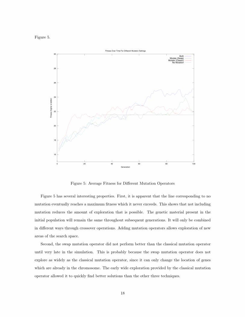
Figure 5.

16

18

20

22

24

26

28

30

0 20 40 60 80 100

Fitn

ess (

hig

he

r is

be

tte

r)

Generation

Fitness Over Time For Different Mutation Settings

BothMutate (Swap)

Mutate (Classic)No Mutation

Figure 5: Average Fitness for Different Mutation Operators

Figure 5 has several interesting properties. First, it is apparent that the line corresponding to no

mutation eventually reaches a maximum fitness which it never exceeds. This shows that not including

mutation reduces the amount of exploration that is possible. The genetic material present in the

initial population will remain the same throughout subsequent generations. It will only be combined

in different ways through crossover operations. Adding mutation operators allows exploration of new

areas of the search space.

Second, the swap mutation operator did not perform better than the classical mutation operator

until very late in the simulation. This is probably because the swap mutation operator does not

explore as widely as the classical mutation operator, since it can only change the location of genes

which are already in the chromosome. The early wide exploration provided by the classical mutation

operator allowed it to quickly find better solutions than the other three techniques.

18

Finally, the combination of both mutation operators was better than either one by itself. Perhaps

it benefited from the larger search provided by the classical mutation operator, while later benefiting

from the more subtle changes performed by the swap mutation operator. It would be interesting

to make the probabilities of either mutation technique a function of time. The classical mutation

operator could be applied more frequently at the end, while the swap mutation operator could be

applied more frequently at the end to explore variations of already successful solutions.

4.2 Mutation Rate

Having determined that the combination of normal mutation and swap mutation gives better perfor-

mance in this problem domain in section 4.1, the effect of changing the probability of mutation will

be considered. The two probabilities pMutate and pMutateSwap will be set to the same value. This

value, p, will be set to 0, 0.05, 0.10, 0.15, and 0.50. One-point crossover will be used. Four trials for

each mutation rate will be performed, and the average fitness from each generation in each of the four

trials will be recorded. The experiments are run with the same plug-in configuration used before, so

it is difficult for the algorithm to produce a chromosome with perfect fitness.

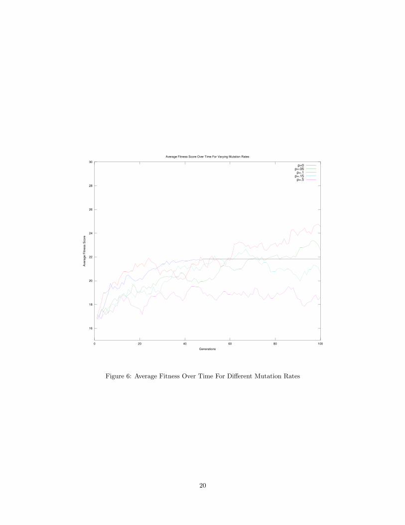
The results of these experiments are shown in Figure 6. Clearly, the selection of the mutation rate

affects the quality of the chromosomes produced by the genetic algorithm. The worst performance

was achieved with p = .5, while the best performance was achieved with p = .1. Since the best

performance was achieved by a mutation rate in the middle of the test values, values above and below

this value should be considered separately.

Those mutation values below p = .1 (p = 0, p = 0.05) produced worse performance. This can be

attributed to reduced exploration of the search space because of less frequent mutation. In the case of

p = 0, the algorithm eventually converged on a single solution with a relatively low fitness. Without

mutation, it was not possible to explore further solutions through crossover operations only.

Higher mutation values also produced worse performance. In this case, it is likely that good

solutions will be subjected to mutations, destroying them. One way to address this problem would

be to make the probability of mutation depend on the fitness of the individual, to reduce the chance

that good solutions will be destroyed by excessive mutation. Increasing the population size might also

help in this situation, since it will increase the probability that more good solutions survive.

The best mutation rate in this case is probably not the best mutation rate for other problems, or

even for the same problem with a different plug-in table. In practice, this rate should be adjusted to

19

16

18

20

22

24

26

28

30

0 20 40 60 80 100

Ave

rag

e F

itn

ess S

co

re

Generations

Average Fitness Score Over Time For Varying Mutation Rates

p=0p=.05p=.1

p=.15p=.5

Figure 6: Average Fitness Over Time For Different Mutation Rates

20

the value which gives the best solutions.

4.3 Crossover Method

The genetic algorithm can produce two offspring from two parents using one of three crossover tech-

niques. In order of increasing “mixing,” they are one-point crossover, two-point crossover, and uniform

crossover. The algorithm will be run using pMutate = pMutateSwap = 0.1, a population of 32 in-

dividuals, and 100 generations. For each of the crossover operations, four trials will be conducted.

The average fitness score of the population over time will be averaged for each of these four trials,

producing three graphs. These graphs will be compared to determine the best crossover strategy for

this problem domain.

16

18

20

22

24

26

28

30

10 20 30 40 50 60 70 80 90 100

Ave

rag

e F

itn

ess

Generations

Average Fitness Over Time For Different Crossover Operations

One-Point CrossoverTwo-Point Crossover

Uniform Crossover

Figure 7: Average fitness scores over time for different crossover techniques

Figure 7 shows the average fitness score of a populations over time given different crossover tech-

niques. The graph does not give a definitive indication of which crossover technique is to be preferred

21

here. Uniform crossover produced the best result in the end, and showed a slow, steady development of

the population from lower fitness to higher fitness over time. One-point crossover rose very quickly at

the beginning of the simulation, but then showed instability in the fitness scores over time. Two-point

crossover was more stable than one-point crossover, but did not ultimately produce a population as

fit as the population created using uniform crossover.

I suspect that these results are highly sensitive to the composition of the randomly generated

initial population. An area of further exploration would be to provide a mechanism for saving the

initial population so that these experiments could be run under more similar conditions each time.

4.4 Selection Method

Two methods of selecting which chromosomes to use for reproduction are compared. Proportional

selection bases the probability of selection on the fitness score, with fitter individuals being more likely

to be selected. Elitism selection selects the fittest half of the population, completely excluding the

least fit individuals. In general, elitism can often restrict the search space because it prevents genetic

information from less fit individuals from being combined with other genetic information, potentially

giving more fit individuals. However, in this case, elitism turned out to be the best selection method.

In this case, elitism clearly out-performs proportional selection. Elitism exerts a much stronger

selective pressure on the population, giving a much steeper rise in average fitness over time. Eventually,

the population reached a maximum average fitness of slightly under 30. In fact, a few chromosomes in

the populations did reach a “perfect score” of 30, however they did not survive to the final generation.

Elitist selection does not distinguish between the best chromosome and the median chromosome, so

there was no pressure to select for the optimal solution. Eventually mutation was applied to the

perfect individuals, decreasing their fitness. In practice, the algorithm could be modified to detect

such individuals and end the algorithm. However, here the simulation was allowed to run for 100

generations no matter what fitness scores were achieved.

I observed that the data from the run with elitism selection reached a maximum value and became

flat, while the data from the run with proportional selection continued gradually increasing over

time through the entire run. Suspecting that I did not allow the simulation to run long enough for

proportional selection to produce a more fit population, I allowed the simulation to run for 10,000

generations. Generation 1858 eventually achieved an average fitness score of 29.82, which is comparable

to the performance of the run using elitism selection. However, it took much longer to achieve this

22

16

18

20

22

24

26

28

30

10 20 30 40 50 60 70 80 90 100

Ave

rag

e F

itn

ess

Generations

Average Fitness Over Time For Different Selection Operators

Proportional SelectionElitism Selection

Figure 8: Comparison of proportional selection and elitism selection operators

23

level of success.

This shows the greater selection pressure imposed by elitism. However, this selection pressure

comes at the price of decreased genetic diversity. In this problem domain, there are a large number

of valid solutions, so the increased search-space exploration provided by this diversity might not be

necessary to find a good solution. In this case, elitism causes rapid convergence on good solutions. In

other problem domains with fewer valid solutions, elitism might exclude regions of the search-space

which contain the best solutions.

5 Conclusion

The most difficult part of this project was the development of the fitness function. It required modeling

a complex system, and is based on a number of simplifying assumptions, particularly with respect to

the network. The utility of the solutions generated by this algorithm could be improved by refining the

fitness function so that it more closely reflects the actual performance possible in the video processing

network. However, based on the data I was able to collect, the fitness function models the network

reasonably well. For the purpose of exploring genetic algorithms, the fitness function provides a

complex feature space with conflicting goals. I suspect that this made it easy to see the difference

between some of the configurations that I tried in my experiments. For example, the difference in

behavior of elitism selection and proportional selection was very apparent.

The comparison of various mutation methods, including one which was created because I suspected

it would be useful for this problem, was interesting. It showed that not using mutation limited the

maximum fitness that could be achieved, while using both mutation operators in concert gave better

results than either one in isolation. In this case, increased searching gave better results. When different

mutation rates were compared, however, it became apparent that too much searching could also be

a problem. A mutation rate which is too high has a tendency to destroy information contained in

successful individuals. The examination of one-point, two-point and uniform crossover also showed

that this can have an effect on the performance of the genetic algorithm. However, it was not clear

from the data I was able to collect which of the crossover techniques is the best to use in this case.

This could be an area for further exploration. Finally, the most surprising result was that elitist

selection gave better results than proportional selection in less time. The conventional wisdom seems

to be that elitism limits the ultimate success of the algorithm by excluding useful genetic material,

24

but in this case the increased selection pressure seems to have been more important.

25