U.S. Department of the InteriorU.S. Geological Survey

Techniques and Methods 7-A2

Prepared in cooperation with Bureau of Land Management and the National Renewable Energy Laboratory

GenEst Statistical Models—A Generalized Estimator of Mortality

Chapter 2 ofSection A, AlgorithmBook 7, Automated Data Processing and Computations

GenEst Statistical Models—A Generalized Estimator of Mortality

By Daniel Dalthorp, Lisa Madsen, Manuela Huso, Paul Rabie, Robert Wolpert, Jared Studyvin, Juniper Simonis, and Jeffrey Mintz

Chapter 2 of Section A, Algorithms Book 7, Automated Data Processing and Computations

Prepared in cooperation with Bureau of Land Management and the National Renewable Energy Laboratory

Techniques and Methods 7-A2

U.S. Department of the Interior U.S. Geological Survey

U.S. Department of the Interior RYAN K. ZINKE, Secretary

U.S. Geological Survey James F. Reilly II, Director

U.S. Geological Survey, Reston, Virginia: 2018

For more information on the USGS—the Federal source for science about the Earth, its natural and living resources, natural hazards, and the environment—visit https://www.usgs.gov/ or call 1–888–ASK–USGS (1–888–275–8747).

For an overview of USGS information products, including maps, imagery, and publications, visit https:/store.usgs.gov.

Any use of trade, firm, or product names is for descriptive purposes only and does not imply endorsement by the U.S. Government.

Although this information product, for the most part, is in the public domain, it also may contain copyrighted materials as noted in the text. Permission to reproduce copyrighted items must be secured from the copyright owner.

Suggested citation: Dalthorp, D., Madsen, L., Huso, M., Rabie, P., Wolpert, R., Studyvin, J., Simonis, J., and Mintz, J., 2018, GenEst statistical models—A generalized estimator of mortality: U.S. Geological Survey Techniques and Methods, book 7, chap. A2, 13 p., https://doi.org/10.3133/tm7A2.

ISSN 2328-7055 (online)

iii

Contents

Section 1—Introduction ................................................................................................................................. 1 Section 2—Splitting Mortality Estimates by Carcass and Recombining into Subgroups ................................ 3 Section 3—Temporal Splits ........................................................................................................................... 4 Section 4—Estimation of Arrival Probabilities ................................................................................................ 6 Section 5—Uncertainty in Estimating 𝑀𝑀|(𝑋𝑋,𝑔𝑔) ............................................................................................ 8 Section 6—Accounting for Unsearched Area ............................................................................................... 10 Section 7—Searcher Efficiency ................................................................................................................... 11 Section 8—Carcass Persistence ................................................................................................................. 13 References Cited ......................................................................................................................................... 13

Abbreviations

𝐀𝐀 𝑋𝑋 × 𝑛𝑛𝑛𝑛𝑛𝑛𝑛𝑛 array of simulated arrival intervals 𝐴𝐴𝑗𝑗 event that the carcass arrived in interval 𝑗𝑗 (between times 𝑡𝑡𝑗𝑗−1 and 𝑡𝑡𝑗𝑗) CDF cumulative distribution function CP carcass persistence 𝑑𝑑𝑑𝑑𝑝𝑝𝑢𝑢 density-weighted proportion or the fraction of carcasses arriving within the searched area at search unit 𝑢𝑢 𝑓𝑓 sampling fraction or the fraction of carcasses at a site that fall at the units selected for search EoA Evidence of Absence software and statistical model 𝑔𝑔, 𝑔𝑔� carcass detection probability, estimated carcass detection probability for carcasses arriving in searched areas GenEst Generalized Estimator of Mortality software and statistical model 𝐼𝐼𝑗𝑗 𝑡𝑡𝑗𝑗 − 𝑡𝑡𝑗𝑗−1 = length of search interval 𝑗𝑗 𝑘𝑘 fractional change in searcher efficiency with each successive search after carcass arrival 𝑀𝑀, 𝑀𝑀� mortality, estimated mortality 𝑛𝑛𝑛𝑛𝑛𝑛𝑛𝑛𝑛𝑛𝑛𝑛ℎ number of carcass search days during the monitored period 𝑛𝑛𝑛𝑛𝑛𝑛𝑛𝑛 number of simulation replicates for accounting for variance 𝑂𝑂𝑖𝑖 event that the carcass is observed in search 𝑛𝑛 (at time 𝑡𝑡𝑖𝑖) 𝑝𝑝 searcher efficiency for carcasses in the first search after carcass arrival SE searcher efficiency 𝑆𝑆(𝑡𝑡) carcass persistence distribution giving the probability a carcass persists 𝑡𝑡 or more days after carcass arrival 𝑡𝑡𝑗𝑗 time (in days) of the 𝑗𝑗th search after the start of monitoring 𝑋𝑋 number of carcasses observed

iv

This page left intentionally blank

1

GenEst Statistical Models—A Generalized Estimator of Mortality

By Daniel Dalthorp1, Lisa Madsen2, Manuela Huso1, Paul Rabie3, Robert Wolpert4, Jared Studyvin3, Juniper Simonis5, and Jeffrey Mintz1

Section 1—Introduction

GenEst (a generalized estimator of mortality) is a suite of statistical models and software tools

for generalized mortality estimation. It was specifically designed for estimating the number of bird and

bat fatalities at solar and wind power facilities, but both the software (Dalthorp and others, 2018) and

the underlying statistical models are general enough to be useful in various situations to estimate the

size of open populations when detection probabilities and search coverages are less than 1. In this

report, we outline the statistical models and data structures underlying the estimator. The models are

numerous, complex, and intricately interwoven. Discussion begins with broad, high-level overviews of

the general models. The lower-level technical details are then gradually added. Broader and less

technical discussions on the general context and applications of the models and the use of the software

are available in the software user guide (Simonis and others, 2018), vignettes bundled with the software,

and the help files within the software itself.

1U.S. Geological Survey. 2Oregon State University. 3Western EcoSystems Technology, Inc. 4Duke University 5DAPPER Stats.

2

At its core, GenEst is an elaboration of a binomial probability model 𝑋𝑋 ~ binomial(𝑀𝑀,𝑔𝑔),

where 𝑋𝑋 is the observed number of carcasses and 𝑔𝑔 is the detection probability. If 𝑔𝑔 is known, then 𝑀𝑀� =

𝑋𝑋/𝑔𝑔 is an unbiased estimator for 𝑀𝑀 and the sampling variance of 𝑋𝑋 is the only source of uncertainty

about 𝑀𝑀. In a slightly more complicated scenario in which total mortality is split into two groups, 𝐴𝐴 and

𝐵𝐵, then 𝑀𝑀� = 𝑀𝑀�𝐴𝐴 + 𝑀𝑀�𝐵𝐵 = 𝑋𝑋𝐴𝐴𝑔𝑔𝐴𝐴

+ 𝑋𝑋𝐵𝐵𝑔𝑔𝐵𝐵

is unbiased for 𝑀𝑀. GenEst makes extensive use of this simple idea of

splitting the carcass observation data into distinct subgroups, estimating mortality in each subgroup, and

combining subgroups into larger groups by summing. A number of technical difficulties must be

overcome to make this simple idea work as a complete estimator that produces accurate confidence

intervals, including accounting for the dependence of 𝑔𝑔 on the time of carcass arrival, estimating 𝑔𝑔 as a

function of covariates, characterizing the uncertainty in 𝑔𝑔�, accounting for correlation structure of the 𝑔𝑔�'s

among various subgroups, accounting for uncertainty in estimating 𝑀𝑀 given 𝑋𝑋 and 𝑔𝑔, and accounting for

unsearched area. GenEst provides solutions for each of these difficulties. The technical details are

lengthy but are fully explained in sections 2–8.

3

Section 2—Splitting Mortality Estimates by Carcass and Recombining into Subgroups

For each carcass, 𝑥𝑥 = 1, … ,𝑋𝑋, that is discovered in carcass surveys, its contribution to the

estimated total mortality is the reciprocal of its inclusion probability, 1/𝑔𝑔𝑥𝑥. However, that contribution

is subject to two types of uncertainty: (1) uncertainty associated with estimating 𝑔𝑔𝑥𝑥 (sections 7–8), and

(2) the uncertainty associated with estimating 𝑀𝑀𝑥𝑥|𝑔𝑔𝑥𝑥 (section 5). We account for the uncertainties using

parametric bootstrapping, that is, simulating from the asymptotic distributions of the maximum

likelihood estimators of parameters. The result is stored in an 𝑋𝑋 × 𝑛𝑛𝑛𝑛𝑛𝑛𝑛𝑛 matrix of carcass contributions

to the estimated total mortality:

𝐌𝐌� =

⎣⎢⎢⎡𝑛𝑛�1,1 𝑛𝑛�1,2 ⋯ 𝑛𝑛�1,𝑛𝑛𝑛𝑛𝑖𝑖𝑛𝑛𝑛𝑛�2,1 𝑛𝑛�2,1 ⋯ 𝑛𝑛�2,𝑛𝑛𝑛𝑛𝑖𝑖𝑛𝑛⋮ ⋮ ⋱ ⋮

𝑛𝑛�𝑋𝑋,1 𝑛𝑛�𝑋𝑋,2 ⋯ 𝑛𝑛�𝑋𝑋,𝑛𝑛𝑛𝑛𝑖𝑖𝑛𝑛⎦⎥⎥⎤ .

Each column of 𝐌𝐌� represents a single realization of the simulated contributions of all the discovered

carcasses to the estimated total mortality. Uncertainty is captured in the distinctions among columns.

Mortality estimation by carcass group is accomplished by subsetting the rows and then taking

column sums. For example, total mortality (no subsetting) is estimated by taking column sums over all

the carcasses to create a vector of estimates, 𝑀𝑀�𝑡𝑡𝑡𝑡𝑡𝑡𝑡𝑡𝑡𝑡 = (∑ 𝑛𝑛�𝑥𝑥,1𝑥𝑥 ,∑ 𝑛𝑛�𝑥𝑥,2𝑥𝑥 , … ,∑ 𝑛𝑛�𝑥𝑥,𝑛𝑛𝑛𝑛𝑖𝑖𝑛𝑛𝑥𝑥 ), from a

parametric bootstrap from the sampling distribution of 𝑀𝑀� . The 𝐌𝐌� matrix can be subsetted to estimate

mortality among desired subgroups in a similar way. For example, to estimate mortality for species B,

calculate 𝑀𝑀�B = (∑ 𝑛𝑛�𝑥𝑥,1𝑥𝑥∈B ,∑ 𝑛𝑛�𝑥𝑥,2𝑥𝑥∈B , … ,∑ 𝑛𝑛�𝑥𝑥,𝑛𝑛𝑛𝑛𝑖𝑖𝑛𝑛𝑥𝑥∈B ), where 𝑥𝑥 ∈ B indicates that carcass 𝑥𝑥 belongs

to species B. GenEst extracts sample statistics (such as median and confidence intervals) from these

empirical 𝑀𝑀� vectors to summarize mortality estimates for subgroups or "splits" as defined by the user.

4

Section 3—Temporal Splits

GenEst can also split mortality estimates by user-specified time intervals or by temporal

covariates such as season. To split the 𝐌𝐌� matrix by carcass arrival times, GenEst relies on an 𝑋𝑋 × 𝑛𝑛𝑛𝑛𝑛𝑛𝑛𝑛

matrix of simulated arrival intervals, 𝐀𝐀, to construct an 𝑛𝑛𝑡𝑡𝑛𝑛𝑛𝑛𝑛𝑛𝑛𝑛 × 𝑛𝑛𝑛𝑛𝑛𝑛𝑛𝑛 array of mortality estimates by

time interval, 𝑀𝑀�𝑇𝑇 , as:

𝐌𝐌�𝑻𝑻 = �∑ 𝑛𝑛�𝑥𝑥,1𝑥𝑥∈𝐼𝐼1 ⋯ ∑ 𝑛𝑛�𝑥𝑥,𝑛𝑛𝑛𝑛𝑖𝑖𝑛𝑛𝑥𝑥∈𝐼𝐼1

⋮ ⋱ ⋮∑ 𝑛𝑛�𝑥𝑥,1𝑥𝑥∈𝐼𝐼𝑛𝑛𝑛𝑛𝑛𝑛𝑛𝑛𝑛𝑛𝑛𝑛 ⋯ ∑ 𝑛𝑛�𝑥𝑥,𝑛𝑛𝑛𝑛𝑖𝑖𝑛𝑛𝑥𝑥∈𝐼𝐼𝑛𝑛𝑛𝑛𝑛𝑛𝑛𝑛𝑛𝑛𝑛𝑛

�,

where 𝑥𝑥 ∈ 𝐼𝐼𝑗𝑗 indicates that the simulated arrival time of carcass 𝑥𝑥 is within the specified interval,𝑗𝑗. If the

simulated arrival interval of a carcass 𝑥𝑥𝑖𝑖 intersects two or more of the splitting intervals (for example, 𝐼𝐼𝑗𝑗

and 𝐼𝐼𝑗𝑗−1), the contribution of the carcass to estimated mortality, 𝑛𝑛� , is allocated proportionally to the

intersecting splitting intervals.

To understand the structure of the 𝐀𝐀 matrix, first note that detection probability for a carcass

depends partly on its arrival time. For example, if monitoring runs from April 1 through October 31,

carcasses arriving near the end of October may be available for discovery for only one or two searches,

whereas carcasses arriving in April may be available for many searches. Search conditions also may

vary with season. However, although carcass discovery times are recorded, arrival times are not known.

Discovered carcasses may have arrived sometime after the previous search or in any search interval

prior to that. Although arrival times cannot be known with certainty, GenEst analyzes the search data to

derive probability distributions of arrival times for each carcass and, from these, creates an 𝑋𝑋 × 𝑛𝑛𝑛𝑛𝑛𝑛𝑛𝑛

matrix of simulated arrival intervals, 𝐀𝐀. For example, if 𝑋𝑋 = 3 and the carcasses were discovered on

searches 𝑛𝑛 = 1, 3, and 12, respectively, and 𝑛𝑛𝑛𝑛𝑛𝑛𝑛𝑛 = 10, the arrival matrix, 𝐀𝐀, might look like the

following:

𝐀𝐀 = �1 1 1 1 1 1 1 1 1 13 3 2 3 1 3 3 3 2 1

12 11 12 10 9 12 12 12 12 11�

5

The simulated arrival intervals for the first carcass are identically 1 because the carcass was discovered

on the first search (at 𝑡𝑡1) and is assumed to have arrived in the first search interval, (𝑡𝑡0, 𝑡𝑡1]. In practice,

the assumption that all carcasses discovered in carcass surveys arrived after 𝑡𝑡0 is often enforced by

disregarding carcasses found in a careful clean-out search at 𝑡𝑡0. The second carcass was discovered in

search 3. According to the arrival probabilities, the carcass was more likely to have arrived in interval 3

than in any other interval, but there is a chance it arrived as early as the first interval, as indicated by the

row of simulated arrivals. The third carcass was found on the 12th search and, in theory, could have

arrived in any interval prior to its discovery. However, it is highly unlikely that it arrived more than a

few intervals prior to the 12th search because, if it had, chances are that it would have been removed by

scavengers or previously found by searchers.

6

Section 4—Estimation of Arrival Probabilities

Suppose searches are conducted at times, 𝑡𝑡0, 𝑡𝑡1, … , 𝑡𝑡𝑛𝑛𝑛𝑛𝑛𝑛𝑡𝑡𝑛𝑛𝑛𝑛ℎ. For each carcass discovered in

carcass surveys 𝑛𝑛 = 1, … ,𝑛𝑛𝑛𝑛𝑛𝑛𝑛𝑛𝑛𝑛𝑛𝑛ℎ, define 𝑂𝑂𝑖𝑖 as the event that the carcass was observed during search 𝑛𝑛

(at time 𝑡𝑡𝑖𝑖) and 𝐴𝐴𝑗𝑗 as the event that the carcass arrived in interval 𝑗𝑗 = �𝑡𝑡𝑗𝑗−1, 𝑡𝑡𝑗𝑗�, 𝑗𝑗 ≤ 𝑛𝑛. The probability

that the carcass arrived in interval 𝑗𝑗 then can be estimated as:

Pr (𝐴𝐴𝑗𝑗|𝑂𝑂𝑖𝑖) =Pr(𝑂𝑂𝑖𝑖|𝐴𝐴𝑗𝑗)Pr (𝐴𝐴𝑗𝑗)

∑ Pr(𝑂𝑂𝑖𝑖|𝐴𝐴𝑗𝑗)Pr (𝐴𝐴𝑗𝑗)𝑗𝑗≤𝑖𝑖

In theory, Pr�𝐴𝐴𝑗𝑗|𝑂𝑂𝑖𝑖� is positive for 𝑗𝑗 = 𝑛𝑛, 𝑛𝑛 − 1, … ,1, but, in practice, Pr�𝐴𝐴𝑗𝑗|𝑂𝑂𝑖𝑖� decreases rapidly to 0

with 𝑗𝑗, so in most cases only the first few terms need to be calculated. The default for GenEst software

is to calculate arrival probabilities for as many as eight intervals prior to discovery, but the R command-

line user may override the default in functions estM and estg. GenEst makes a further assumption that

the arrival rate is constant in the search intervals preceding carcass arrival, so

Pr�𝐴𝐴𝑗𝑗�𝑂𝑂𝑖𝑖� =Pr(𝑂𝑂𝑖𝑖|𝐴𝐴𝑗𝑗)/𝐼𝐼𝑗𝑗

∑ Pr(𝑂𝑂𝑖𝑖|𝐴𝐴𝑗𝑗) Pr�𝐴𝐴𝑗𝑗� /𝐼𝐼𝑗𝑗𝑗𝑗≤𝑖𝑖

where 𝐼𝐼𝑗𝑗 = 𝑡𝑡𝑗𝑗 − 𝑡𝑡𝑗𝑗−1 = length of interval 𝑗𝑗.

The estimator is robust to variation in arrival rates among different search intervals provided

there is not an abrupt change in arrival rate from one interval to the next. However, even in these

unusual conditions, the potential for bias in estimating total mortality would be small because the same

pattern would need to recur with a large fraction of the carcasses. The potential for bias would be further

attenuated by high searcher efficiency [SE] or low persistence times.

7

Calculation of Pr�𝐴𝐴𝑗𝑗�𝑂𝑂𝑖𝑖� is based on calculation of Pr(𝑂𝑂𝑖𝑖|𝐴𝐴𝑗𝑗):

Pr�𝑂𝑂𝑛𝑛�𝐴𝐴𝑗𝑗� =

⎩⎪⎪⎨

⎪⎪⎧

0, 𝑛𝑛 < 𝑗𝑗

𝑝𝑝�𝑆𝑆(𝑡𝑡𝑛𝑛 − 𝑡𝑡)

𝐼𝐼𝑗𝑗𝑑𝑑𝑡𝑡

𝑡𝑡𝑗𝑗

𝑡𝑡𝑗𝑗−1

, 𝑛𝑛 = 𝑗𝑗

�� (1− 𝑝𝑝𝑘𝑘𝑛𝑛)𝑛𝑛−𝑗𝑗−1

𝑛𝑛=0� 𝑝𝑝𝑘𝑘𝑛𝑛−𝑗𝑗 �

𝑆𝑆(𝑡𝑡𝑛𝑛 − 𝑡𝑡)𝐼𝐼𝑗𝑗

𝑑𝑑𝑡𝑡𝑡𝑡𝑗𝑗

𝑡𝑡𝑗𝑗−1

, 𝑛𝑛 > 𝑗𝑗

where 𝑆𝑆(𝑡𝑡) is the probability that a carcass persists 𝑡𝑡 days after arrival (section 8), 𝑝𝑝 and 𝑘𝑘 are searcher

efficiency parameters (section 7), and 𝑛𝑛 (the index on the product) runs from the search interval

immediately before carcass discovery to the first search interval of the monitored period. A carcass may

arrive in one season and be discovered in a later season after search conditions have changed. To

account for this possibility, in the calculation of Pr�𝑂𝑂𝑖𝑖| 𝐴𝐴𝑗𝑗� of a carcass for a given 𝑗𝑗, the carcass is

assigned the search characteristics appropriate to the assumed arrival interval, 𝑗𝑗. For example, if a

carcass is discovered on the first search in the autumn, and search conditions (that is, SE and carcass

persistence [CP] parameters) change from summer to autumn, then Pr(𝑂𝑂𝑖𝑖| 𝐴𝐴𝑖𝑖) is calculated with the

autumn SE and CP parameters and Pr(𝑂𝑂𝑖𝑖| 𝐴𝐴𝑖𝑖−1) is calculated with the summer parameters.

Arrival-interval probabilities, Pr�𝐴𝐴𝑗𝑗| 𝑂𝑂𝑖𝑖�, are calculated for each carcass and search interval, and

an integer-valued 𝑋𝑋 × 𝑛𝑛𝑛𝑛𝑛𝑛𝑛𝑛 matrix of simulated arrival intervals, 𝐀𝐀, is constructed. Each column

represents the arrival interval of each carcass in a simulated set of carcass arrivals. In other words, each

column represents simulated arrival intervals of the set of observed carcasses over the course of one

field season or simulated "year". As mentioned previously, carcass detection probabilities depend on

arrival times, which are given in the arrival matrix 𝐀𝐀. For each simulated year (column in 𝐀𝐀), the

detection probability for each carcass is estimated as

𝑔𝑔� = Pr�𝑂𝑂|𝐴𝐴𝑗𝑗� = � Pr �𝑂𝑂𝑖𝑖| 𝐴𝐴𝑗𝑗�𝑖𝑖

to construct an 𝑋𝑋 × 𝑛𝑛𝑛𝑛𝑛𝑛𝑛𝑛 matrix, 𝑔𝑔�, of carcass detection probabilities that are applicable to the carcass

at the time of carcass arrival. For example, 𝑔𝑔�𝑥𝑥,𝑗𝑗 is a simulated inclusion probability of carcass 𝑥𝑥,

assuming it arrived in interval 𝐴𝐴𝑥𝑥,𝑗𝑗.

8

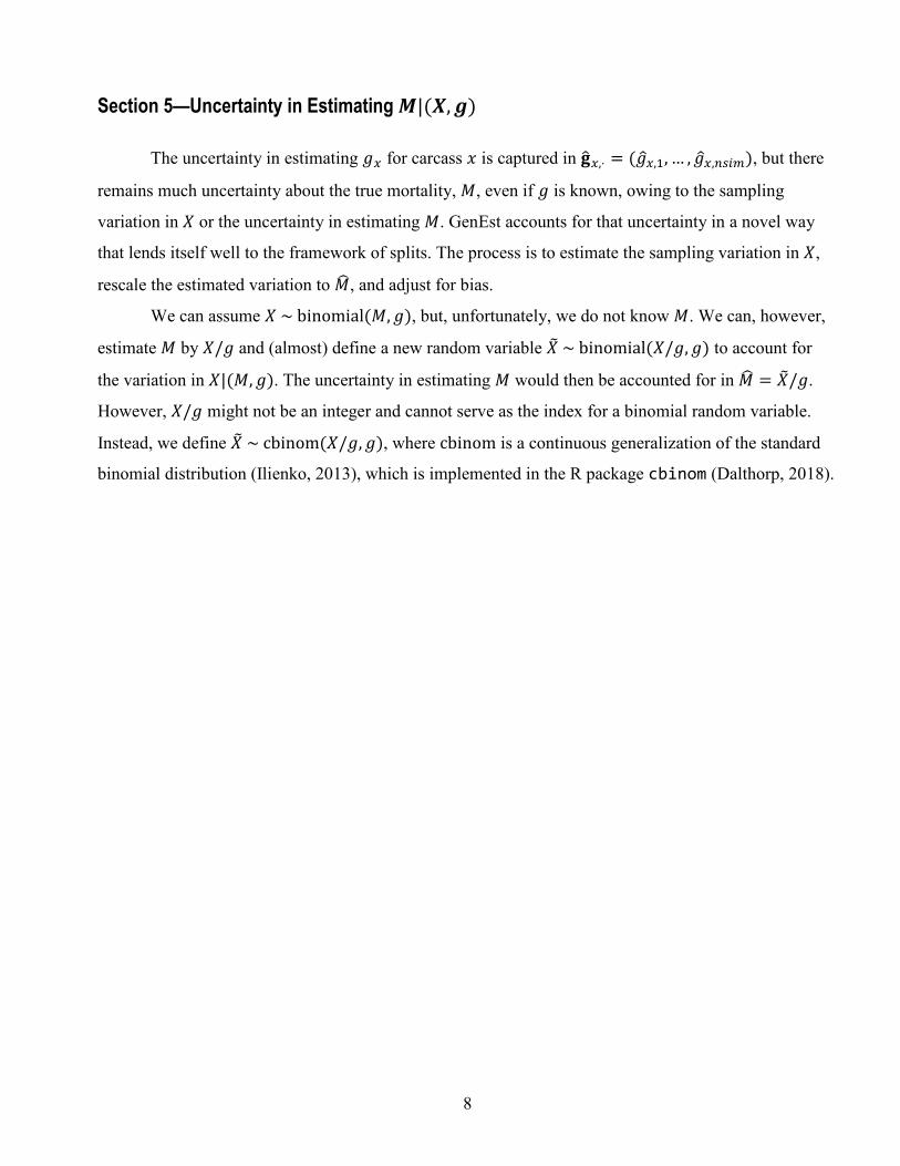
Section 5—Uncertainty in Estimating 𝑴𝑴|(𝑿𝑿,𝒈𝒈)

The uncertainty in estimating 𝑔𝑔𝑥𝑥 for carcass 𝑥𝑥 is captured in 𝐠𝐠�𝑥𝑥,⋅ = (𝑔𝑔�𝑥𝑥,1, … ,𝑔𝑔�𝑥𝑥,𝑛𝑛𝑛𝑛𝑖𝑖𝑛𝑛), but there

remains much uncertainty about the true mortality, 𝑀𝑀, even if 𝑔𝑔 is known, owing to the sampling

variation in 𝑋𝑋 or the uncertainty in estimating 𝑀𝑀. GenEst accounts for that uncertainty in a novel way

that lends itself well to the framework of splits. The process is to estimate the sampling variation in 𝑋𝑋,

rescale the estimated variation to 𝑀𝑀� , and adjust for bias.

We can assume 𝑋𝑋 ~ binomial(𝑀𝑀,𝑔𝑔), but, unfortunately, we do not know 𝑀𝑀. We can, however,

estimate 𝑀𝑀 by 𝑋𝑋/𝑔𝑔 and (almost) define a new random variable 𝑋𝑋� ~ binomial(𝑋𝑋/𝑔𝑔,𝑔𝑔) to account for

the variation in 𝑋𝑋|(𝑀𝑀,𝑔𝑔). The uncertainty in estimating 𝑀𝑀 would then be accounted for in 𝑀𝑀� = 𝑋𝑋�/𝑔𝑔.

However, 𝑋𝑋/𝑔𝑔 might not be an integer and cannot serve as the index for a binomial random variable.

Instead, we define 𝑋𝑋� ~ cbinom(𝑋𝑋/𝑔𝑔,𝑔𝑔), where cbinom is a continuous generalization of the standard

binomial distribution (Ilienko, 2013), which is implemented in the R package cbinom (Dalthorp, 2018).

9

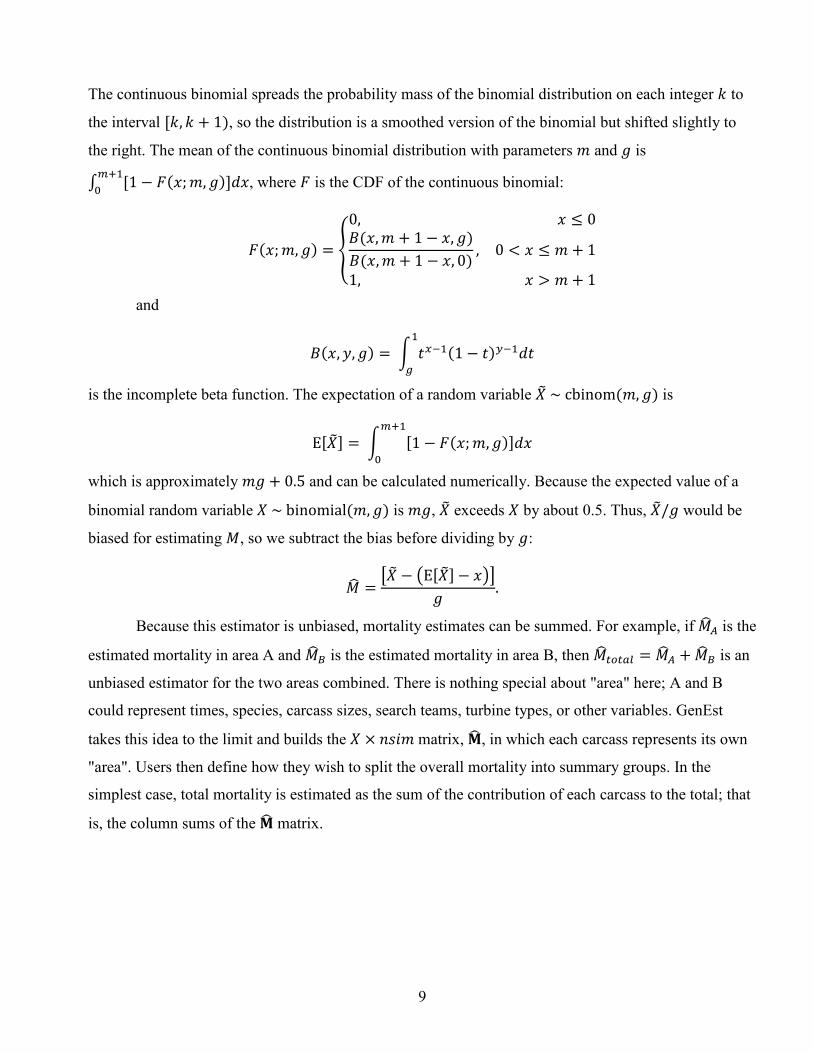
The continuous binomial spreads the probability mass of the binomial distribution on each integer 𝑘𝑘 to

the interval [𝑘𝑘,𝑘𝑘 + 1), so the distribution is a smoothed version of the binomial but shifted slightly to

the right. The mean of the continuous binomial distribution with parameters 𝑛𝑛 and 𝑔𝑔 is

∫ [1 − 𝐹𝐹(𝑥𝑥;𝑛𝑛,𝑔𝑔)]𝑑𝑑𝑥𝑥𝑛𝑛+10 , where 𝐹𝐹 is the CDF of the continuous binomial:

𝐹𝐹(𝑥𝑥;𝑛𝑛,𝑔𝑔) = �

0, 𝑥𝑥 ≤ 0𝐵𝐵(𝑥𝑥,𝑛𝑛 + 1 − 𝑥𝑥,𝑔𝑔)𝐵𝐵(𝑥𝑥,𝑛𝑛 + 1 − 𝑥𝑥, 0)

, 0 < 𝑥𝑥 ≤ 𝑛𝑛 + 1

1, 𝑥𝑥 > 𝑛𝑛 + 1

and

𝐵𝐵(𝑥𝑥,𝑦𝑦,𝑔𝑔) = � 𝑡𝑡𝑥𝑥−1(1 − 𝑡𝑡)𝑦𝑦−1𝑑𝑑𝑡𝑡1

𝑔𝑔

is the incomplete beta function. The expectation of a random variable 𝑋𝑋� ~ cbinom(𝑛𝑛,𝑔𝑔) is

E[𝑋𝑋�] = � [1 − 𝐹𝐹(𝑥𝑥;𝑛𝑛,𝑔𝑔)]𝑑𝑑𝑥𝑥𝑛𝑛+1

0

which is approximately 𝑛𝑛𝑔𝑔 + 0.5 and can be calculated numerically. Because the expected value of a

binomial random variable 𝑋𝑋 ~ binomial(𝑛𝑛,𝑔𝑔) is 𝑛𝑛𝑔𝑔, 𝑋𝑋� exceeds 𝑋𝑋 by about 0.5. Thus, 𝑋𝑋�/𝑔𝑔 would be

biased for estimating 𝑀𝑀, so we subtract the bias before dividing by 𝑔𝑔:

𝑀𝑀� =�𝑋𝑋� − �E[𝑋𝑋�]− 𝑥𝑥��

𝑔𝑔.

Because this estimator is unbiased, mortality estimates can be summed. For example, if 𝑀𝑀�𝐴𝐴 is the

estimated mortality in area A and 𝑀𝑀�𝐵𝐵 is the estimated mortality in area B, then 𝑀𝑀�𝑡𝑡𝑡𝑡𝑡𝑡𝑡𝑡𝑡𝑡 = 𝑀𝑀�𝐴𝐴 + 𝑀𝑀�𝐵𝐵 is an

unbiased estimator for the two areas combined. There is nothing special about "area" here; A and B

could represent times, species, carcass sizes, search teams, turbine types, or other variables. GenEst

takes this idea to the limit and builds the 𝑋𝑋 × 𝑛𝑛𝑛𝑛𝑛𝑛𝑛𝑛 matrix, 𝐌𝐌� , in which each carcass represents its own

"area". Users then define how they wish to split the overall mortality into summary groups. In the

simplest case, total mortality is estimated as the sum of the contribution of each carcass to the total; that

is, the column sums of the 𝐌𝐌� matrix.

10

Section 6—Accounting for Unsearched Area

Unless the user is interested in estimating mortality strictly in the searched area, 𝑔𝑔� values must

be adjusted to account for the unsearched area. In practice, some carcasses are likely to fall outside the

searched area in a given unit (for example, in an unsearched part of a search ring at a solar power tower

facility or beyond the search radius at a wind turbine). For each search unit, 𝑢𝑢, the expected fraction of

carcasses that are killed at the unit but fall outside the searched area is the density-weighted proportion

or 𝑑𝑑𝑑𝑑𝑝𝑝𝑢𝑢 (Huso and Dalthorp, 2014). Additionally, there may be units at a site that are not searched at

all. The expected fraction of carcasses arriving at the units searched at a site is the sampling fraction or

f. For example, if units at a wind facility are the individual turbines, then 𝑓𝑓 would be the fraction of

turbines surveyed. Thus, the contributions of the respective carcasses to the estimate of total mortality

are then summarized in a 𝑋𝑋 × 𝑛𝑛𝑛𝑛𝑛𝑛𝑛𝑛 array as 1𝐝𝐝𝐝𝐝𝐝𝐝⋅𝐠𝐠�⋅𝑓𝑓

, where 𝐝𝐝𝐝𝐝𝐝𝐝 = diag(𝐝𝐝𝐝𝐝𝐝𝐝) is the diagonal matrix of

𝑑𝑑𝑑𝑑𝑝𝑝 values associated with the carcassess. For example, if carcass 1 was found at unit 17 and was a

medium-sized bird, then 𝑑𝑑𝑑𝑑𝑝𝑝1,1 would be the 𝑑𝑑𝑑𝑑𝑝𝑝 for medium-sized birds at unit 17. 𝐌𝐌� would then be

calculated based on this adjusted 𝐠𝐠�∗ = 𝐝𝐝𝐝𝐝𝐝𝐝 ⋅ 𝐠𝐠� ⋅ 𝑓𝑓.

11

Section 7—Searcher Efficiency

Searcher efficiency and carcass persistence (section 8) are estimated from field trials where a

known number of carcasses are placed and their fate (found or scavenged) is recorded. Let 𝑝𝑝 be the

initial SE for fresh carcasses, or, more precisely, the conditional probability of detecting a carcass on the

first search after carcass arrival, given that the carcass is present at the time of the search. Let 𝑘𝑘 be the

fractional change in SE with each successive search. Thus, if SE trial carcasses that are missed in one

search are left in the field for possible discovery on later searches, 𝑝𝑝 and 𝑘𝑘 can be estimated

simultaneously as functions of categorical covariates.

Specifically, let 𝑝𝑝𝑛𝑛 be the probability that carcass 𝑛𝑛 is found during the first search after carcass

arrival given that it is present at the time of the search. The model allows 𝑝𝑝𝑛𝑛 to depend on a vector of

covariates 𝐗𝐗𝑛𝑛 as logit(𝑝𝑝𝑖𝑖) = 𝐗𝐗𝑖𝑖𝛽𝛽, where 𝛽𝛽 is a vector of coefficients associated with combinations of

covariate levels. The model allows a constant multiplicative reduction in detection probability in

subsequent searches. The probability of finding carcass i during search j is

Pr{detect carcass 𝑛𝑛 on occasion 𝑗𝑗} = 𝑝𝑝𝑛𝑛𝑘𝑘𝑛𝑛𝑗𝑗−1

where 𝑘𝑘𝑛𝑛 may also be a logit-linear function of covariates and coefficients. These covariates need not be

the same as those used to model 𝑝𝑝𝑖𝑖.

Consider the search outcome history for a given carcass. If the carcass was scavenged before the

first search occasion, then the carcass provides no information to estimate SE, and the model ignores

these carcasses. If the carcass is present during one or more search occasions, then the probability of its

search history is determined by that history and equation. These relations are easiest to see with a couple

of examples. Suppose carcass 𝑛𝑛 (from the SE field trials) was missed on three searches and detected on

the fourth search. Its search history is then (0, 0, 0, 1) in the notation of the data, and the probability of

this search history is

Pr{(0, 0, 0, 1)} = �1− 𝑝𝑝𝑛𝑛��1− 𝑝𝑝𝑛𝑛𝑘𝑘𝑛𝑛� �1− 𝑝𝑝𝑛𝑛𝑘𝑘𝑛𝑛2�𝑝𝑝𝑛𝑛𝑘𝑘𝑛𝑛

3 = 𝐿𝐿𝑛𝑛

where 𝐿𝐿𝑛𝑛 denotes the contribution of carcass 𝑛𝑛 to the joint likelihood.

12

A carcass may never be found. For example, suppose carcass 𝑛𝑛′ was missed on the first two

search occasions and was then scavenged before the third search. This carcass has search history (0, 0),

and

𝐿𝐿𝑖𝑖′ = (1 − 𝑝𝑝𝑖𝑖′)(1− 𝑝𝑝𝑖𝑖′𝑘𝑘𝑖𝑖′)

The log-likelihood of the data is then expressed as log 𝐿𝐿 = ∑ log 𝐿𝐿𝑖𝑖𝑁𝑁𝑖𝑖=1 , where 𝑁𝑁 denotes the total

number of carcasses in the trial. Let 𝑧𝑧𝑛𝑛 denote the number of zeros in the search history for carcass i

(that is, 𝑧𝑧𝑛𝑛 is the number of times carcass 𝑛𝑛 was missed in searches), and let 𝑓𝑓𝑛𝑛 denote the search

occasion where the carcass was found, with 𝑓𝑓𝑛𝑛 = 0 if the carcass was never found. The, log𝐿𝐿𝑛𝑛 will then

have the form

log𝐿𝐿𝑛𝑛 = � log �1− 𝑝𝑝𝑛𝑛𝑘𝑘𝑛𝑛𝑗𝑗�+ 𝟏𝟏𝑓𝑓𝑛𝑛>0 log �𝑝𝑝𝑛𝑛𝑘𝑘𝑛𝑛

𝑓𝑓𝑛𝑛−1�𝑧𝑧𝑛𝑛−1

𝑗𝑗=0

where 𝟏𝟏𝑓𝑓𝑛𝑛>0 = 1 if 𝑓𝑓𝑛𝑛 > 0 and zero otherwise. Thus, the log-likelihood depends on the data only

through the number of missed searches and whether the carcass was eventually found.

The log-likelihood, 𝐿𝐿, of the data is numerically maximized in using R's optim function. From

the theory of maximum likelihood, the vector of maximum likelihood estimators (MLEs) for the

parameters (𝛽𝛽�) is asymptotically multivariate normal with mean equal to the true parameter values and

variance-covariance matrix given by the inverse information matrix, which is returned by optim as the

hessian.

To account for the uncertainty in estimating 𝑝𝑝 and 𝑘𝑘 parameters, GenEst first approximates the

sampling distribution of 𝛽𝛽� by simulating from the multivariate normal (MVN),

𝛽𝛽�sim~MVN(𝛽𝛽�,𝐇𝐇−1)

Where 𝐇𝐇 is the Hessian matrix returned by optim().

Simulated sampling distributions of 𝑝𝑝𝑖𝑖 and 𝑘𝑘𝑖𝑖 are obtained by back transformation of simulated

�̂�𝛽. Specifically, let 𝐗𝐗𝑖𝑖 represent the covariate vector for the 𝑛𝑛th carcass, then

𝑘𝑘�𝑛𝑛 =1

1 + exp�−𝐗𝐗𝑛𝑛 ⋅ 𝛽𝛽�𝑘𝑘� and 𝑝𝑝�𝑛𝑛 =

11 + exp (−𝐗𝐗𝑛𝑛 ⋅ 𝛽𝛽�𝑝𝑝)

where �̂�𝛽𝑝𝑝 and �̂�𝛽𝑘𝑘 are the components of �̂�𝛽 associated with 𝑝𝑝 and 𝑘𝑘, respectively.

13

Section 8—Carcass Persistence

Carcass persistence times are modeled using censored exponential, Weibull, lognormal, and

loglogistic survival models, which are fit by maximum likelihood estimation using the R functions

survival::survreg (Therneau, 2015) and optim (R Core Team, 2018). Both the location and

scale parameters (Kalbfleisch and Prentice, 2002, chapter 2) may depend on categorical covariates, such

as visibility class, season, or other factors. As with the SE estimates, vectors of simulated persistence

parameters are generated from the fitted models.

References Cited

Dalthorp, D., 2018, cbinom—Continuous analog of a binomial distribution—R package, version 1.3:

Web page accessed October 19, 2018, at https://CRAN.R-project.org/package=cbinom.

Dalthorp, D., Simonis, J., Madsen, L., Huso, M., Rabie, P., Mintz, J., Wolpert, R., Studyvin, J., and

Korner-Nievergelt, F., 2018, GenEst—Generalised fatality estimator—R package, version 1.0.0: Web

page accessed October 19, 2018, at https://code.usgs.gov/ecosystems/GenEst/tags/1.0.0.

Huso, M.M.P., and Dalthorp, D., 2014, Accounting for unsearched areas in estimating wind turbine-

caused fatality: The Journal of Wildlife Management, v. 78, no. 2, p. 347–358.

Ilienko, A., 2013, Continuous counterparts of Poisson and binomial distributions and their properties:

Annales Universitatis Scientarium Budapestinensis, Sectio Computatorica, v. 39: p. 137–147.

Kalbfleisch, J.D., and Prentice, R.L., 2002, The statistical analysis of failure time data: Hoboken, New

Jersey, Wiley, 462 p.

R Core Team, 2018, R—A language and environment for statistical computing: Vienna, Austria, R

Foundation for Statistical Computing web page, accessed October 19, 2018, at https://www.R-

project.org/.

Simonis, J., Dalthorp, D., Huso, M., Mintz, J., Madsen, L., Rabie, P., and Studyvin, J., 2018, GenEst

user guide: Software for a generalized estimator of mortality: U.S. Geological Survey Techniques and

Methods, book 7, chap. C19, 72 p.

Therneau, T., 2015, Package for survival analysis in S, version 2.38: The Comprehensive R Archive

Network web page, accessed October 19, 2018, at https://CRAN.R-project.org/package=survival.

Publishing support provided by the U.S. Geological SurveyScience Publishing Network, Tacoma Publishing Service Center

For more information concerning the research in this report, contact theDirector, Forest and Rangeland Ecosystem Science Center U.S. Geological Survey 777 NW 9th St., Suite 400 Corvallis, Oregon 97330 https://www.usgs.gov/centers/fresc/

Dalthrop and others—G

enEst Statistical Models—

A G

eneralized Estimator of M

ortality—Techniques and M

ethods 7-A2

ISSN 2328-7055 (online)https://doi.org/10.3133/tm7A2