Generic simulation cell method - CORE · Generic simulation cell method ... I present a method for...

GMDD7, 4577–4602, 2014

Generic simulationcell method

I. Honkonen

Title Page

Abstract Introduction

Conclusions References

Tables Figures

J I

J I

Back Close

Full Screen / Esc

Printer-friendly Version

Interactive Discussion

Discussion

Paper

|D

iscussionP

aper|

Discussion

Paper

|D

iscussionP

aper|

Geosci. Model Dev. Discuss., 7, 4577–4602, 2014www.geosci-model-dev-discuss.net/7/4577/2014/doi:10.5194/gmdd-7-4577-2014© Author(s) 2014. CC Attribution 3.0 License.

This discussion paper is/has been under review for the journal Geoscientific ModelDevelopment (GMD). Please refer to the corresponding final paper in GMD if available.

The generic simulation cell method fordeveloping extensible, efficient andreadable parallel computational modelsI. Honkonen1,*

1Heliophysics Science Division, Goddard Space Flight Center, NASA,Greenbelt, Maryland, USA*previously at: Earth Observation, Finnish Meteorological Institute, Helsinki, Finland

Received: 11 June 2014 – Accepted: 30 June 2014 – Published: 18 July 2014

Correspondence to: I. Honkonen ([email protected])

Published by Copernicus Publications on behalf of the European Geosciences Union.

4577

http://www.geosci-model-dev-discuss.net

http://www.geosci-model-dev-discuss.net/7/4577/2014/gmdd-7-4577-2014-print.pdf

http://www.geosci-model-dev-discuss.net/7/4577/2014/gmdd-7-4577-2014-discussion.html

http://creativecommons.org/licenses/by/3.0/

GMDD7, 4577–4602, 2014


I. Honkonen

Title Page



Tables Figures

J I

J I

Back Close

Full Screen / Esc



Discussion

Paper

|D

iscussionP

aper|

Discussion

Paper

|D

iscussionP

aper|

Abstract

I present a method for developing extensible and modular computational models with-out sacrificing serial or parallel performance or source code readability. By usinga generic simulation cell method I show that it is possible to combine several dis-tinct computational models to run in the same computational grid without requiring5

any modification of existing code. This is an advantage for the development and testingof computational modeling software as each submodel can be developed and testedindependently and subsequently used without modification in a more complex cou-pled program. Support for parallel programming is also provided by allowing usersto select which simulation variables to transfer between processes via a Message10

Passing Interface library. This allows the communication strategy of a program tobe formalized by explicitly stating which variables must be transferred between pro-cesses for the correct functionality of each submodel and the entire program. Thegeneric simulation cell class presented here requires a C++ compiler that supportsvariadic templates which were standardized in 2011 (C++11). The code is available15

at: https://github.com/nasailja/gensimcell for everyone to use, study, modify and redis-tribute; those that do are kindly requested to cite this work.

1 Introduction

Computational modeling has become one of the cornerstones of many scientific dis-ciplines, helping to understand observations and to form and test new hypotheses.20

Here a computational model is defined as numerically solving a set of mathematicalequations with one or more variables using a discrete representation of time and themodeled volume. Today the bottleneck of computational modeling is shifting from hard-ware performance towards that of software development, more specifically to the abilityto develop more complex models and to verify and validate them in a timely and cost-25

efficient manner (Post and Votta, 2005). The importance of verification and validation

4578





https://github.com/nasailja/gensimcell

GMDD7, 4577–4602, 2014


I. Honkonen

Title Page



Tables Figures

J I

J I

Back Close

Full Screen / Esc



Discussion

Paper

|D

iscussionP

aper|

Discussion

Paper

|D

iscussionP

aper|

is highlighted by the fact that even a trivial bug can have devastating consequencesnot only for users of the affected software but for others who try to publish contradictingresults (Miller, 2006).

Modular software can be (re)used with minimal modification and is advantageousnot only for reducing development effort but also for verifying and validating a new5

program. For example the number of errors in software components that are reusedwithout modification can be an order of magnitude lower than in components whichare either developed from scratch or modified extensively before use (Thomas et al.,1997). The verification and validation (V & V) of a program consisting of several mod-ules should start from V & V of each module separately before proceeding to combi-10

nations of modules and finally the entire program (Oberkampf and Trucano, 2002).Modules that have been V & V’d and are used without modification increase the con-fidence in the functionality of the larger program and decrease the effort required forfinal V & V.

Reusable software that does not depend on any specific type of data can be written15

by using, for example, generic programming (Musser and Stepanov, 1989). Waligoraet al. (1995) reported that the use of object-oriented design and generics of the Adaprogramming language at Flight Dynamics Division of NASA’s Goddard Space FlightCenter had increased sofware reuse by a factor of three and, in addition to other bene-fits, reduced the error rates and costs substantially. With C++ generic software can be20

developed without sacrificing computational performance through the use of compile-time template parameters for which the compiler can perform optimizations that wouldnot be possible otherwise (Stroustrup, 1999).

Generic and modular software is especially useful for developing complex computa-tional models that couple together several different and possibly independently devel-25

oped codes. From a software development point of view code coupling can be definedas simply making the variables stored by different codes available to each other. Inthis sense even a model for the flow of incompressible, homogeneous and non-viscous

4579





GMDD7, 4577–4602, 2014


I. Honkonen

Title Page



Tables Figures

J I

J I

Back Close

Full Screen / Esc



Discussion

Paper

|D

iscussionP

aper|

Discussion

Paper

|D

iscussionP

aper|

fluid without external forcing

∂v∂t

= −v · (∇v)−∇p; ∇2p = −∇ · (v · (∇v))

where v is velocity and p is pressure, can be viewed as a coupled model as there aretwo equations that can be solved by different solvers. If a separate solver is writtenfor each equation and both solvers are simulating the same volume with identical dis-5

cretization, coupling is only a matter of data exchange. In this work the term solver willbe used when referring to any code/function/module/library which takes as input thedata of a cell and its N neighbors and produces the next state of the cell (next step,iteration, temporal substep, etc.).

The methods of communicating data between solvers can vary widely depending on10

the available development effort, the programming language(s) involved and details ofthe specific codes. Probably the easiest coupling method to develop is to transfer datathrough the filesystem, i.e. at every step each solver writes the data needed by othersolvers into a file and reads the data produced by other solvers from other files. Thismethod is especially suitable as a first version of coupling when the codes have been15

written in different programming languages and use non-interoperable data structures.Performance-wise a more optimal way to communicate between solvers in a coupled

program is to use shared memory, as is done for example in Hill et al. (2004), Jöckelet al. (2005), Larson et al. (2005), Toth et al. (2005), Zhang and Parashar (2006) andRedler et al. (2010), but this technique still has shortcomings. Perhaps the most impor-20

tant one is the fact that the data types used by solvers are not visible to outside, thusmaking intrusive modifications (i.e. modifications to existing code or data structures)necessary in order to transfer data between solvers. The data must be converted toan intermediate format by the solver “sending” the data and subsequently convertedto the internal format by the solver “receiving” the data. The probability of bugs is also25

increased as the code doing the end-to-end conversion is scattered in two differentplaces and the compiler cannot perform static type checking for the final coupled pro-gram. These problems can be alleviated by e.g. writing the conversion code in another

4580





GMDD7, 4577–4602, 2014


I. Honkonen

Title Page



Tables Figures

J I

J I

Back Close

Full Screen / Esc



Discussion

Paper

|D

iscussionP

aper|

Discussion

Paper

|D

iscussionP

aper|

language and outputting the final code of both submodels automatically (Eller et al.,2009). Interpolation between different grids and coordinate systems that many of theframeworks mentioned previously perform can also be viewed as part of the data trans-fer problem but is outside the scope of this work.

A distributed memory parallel program can require significant amounts of code for5

arranging the transfers of different variables between processes, for example, if theamount of data required by some variable(s) changes as a function of both space andtime. The problem is even harder if a program consists of several coupled modelswith different time stepping strategies and/or variables whose memory requirementschange at run time. Futhermore, modifying an existing time stepping strategy or adding10

another model into the program can require substatial changes to existing code in orderto accomodate additional model variables and/or temporal substeps.

1.1 Generic simulation cell method

A generic simulation cell class is presented that provides an abstraction for the storageof simulation variables and the transfer of variables between processes in a distributed15

memory parallel program. Each variable to be stored in the generic cell class is givenas a template parameter to the class. The type of each variable is not restricted inany way by the cell class or solvers developed using this abstraction, enabling genericprogramming in simulation development all the way from the top down to a very lowlevel. By using variadic templates of the 2011 version of the C++ standard, the total20

number of variables is only limited by the compiler implementation and a minimum of1024 is recommended by C++11 (see e.g. Annex B in Du Toit, 2012).

By using the generic cell abstraction it is possible to develop distributed memoryparallel computational models in a way that easily allows one to combine an arbitrarynumber of separate models without modifying any existing code. This is demonstrated25

by combining parallel models for Conway’s Game of Life, scalar advection and La-grangian transport of particles in an external velocity field. In order to keep the pre-sented programs succinct, combining computational models is defined here as running

4581





GMDD7, 4577–4602, 2014


I. Honkonen

Title Page



Tables Figures

J I

J I

Back Close

Full Screen / Esc



Discussion

Paper

|D

iscussionP

aper|

Discussion

Paper

|D

iscussionP

aper|

each model on the same grid structure with identical domain decomposition accrossprocesses. This is not mandatory for the generic cell approach and, for example, thecase of different domain decomposition of submodels is discussed in Sect. 4. Also thedefinition of modifying existing code excludes copying and pasting unmodified codeinto a new file.5

Section 2 introduces the generic simulation cell class concept via a serial implemen-tation and Sect. 3 extends it to distributed memory parallel programs. Section 4 showsthat it is possible to combine three different computational models without modifyingany existing code by using the generic simulation cell method. Section 5 shows that thegeneric cell implementation developed here does not seem to have an adverse effect10

on either serial or parallel computational performance. The code is available at: https://github.com/nasailja/gensimcell for everyone to use, study, modify and redistribute;users are kindly requested to cite this work. The relative paths to source code files givenin the rest of the text refer to the version of the generic simulation cell tagged as 0.5 inthe git repository and is available at: https://github.com/nasailja/gensimcell/tree/0.5/.15

2 Serial implementation

Figure 1 shows a basic implementation of the generic simulation cell class that does notprovide support for MPI applications and is not const-correct but is otherwise complete.The cell class takes as input an arbitrary number of template parameters that corre-spond to variables to be stored in the cell. Each varible only defines its type through20

the name data_type (e.g. lines 5 and 6 in Fig. 2) and is otherwise empty. When thecell class is given one variable as a template argument the code on lines 3..13 is used.The variable given to the cell class as a template parameter is stored as a privatemember of the cell class on line 5 and access to it is provided by the cell’s [] oper-ator overloaded for the variable’s class on lines 8..12. When given multiple variables25

as template arguments the code on lines 15..33 is used which similarly stores the firstvariable as a private member and provides access to it via the [] operator. Additionally

4582








https://github.com/nasailja/gensimcell/tree/0.5/

GMDD7, 4577–4602, 2014


I. Honkonen

Title Page



Tables Figures

J I

J I

Back Close

Full Screen / Esc



Discussion

Paper

|D

iscussionP

aper|

Discussion

Paper

|D

iscussionP

aper|

the cell class derives from from itself with one less variable on line 21. This recursionis stopped by eventually inheriting the one variable version of the cell class. Access tothe private data members representing all variables are provided by the respective []operators which are made available to outside of the cell class on line 26. The memorylayout of variables in an instance of the cell class depends on the compiler implemen-5

tation and can include, for example, padding between variables given as consecutivetemplate parameters. This also applies to variables stored in “ordinary” structures andin both cases if, for example, several values must be stored contiguously in memorya container guaranteeing this should be used such as std::array or std::vector.

Figure 2 shows a complete serial implementation of Conway’s Game of Life (GoL)10

using the generic simulation cell class. A version of this example with console outputis available at: examples/game_of_life/serial.cpp1. Lines 5..7 define the variables to beused in the model and the cell type to be used in the model grid. Lines 10..20 createthe simulation grid and initialize the simulation with a pseudorandom initial condition.The time stepping loop spans lines 22..57. The [] operator is used to obtain a reference15

to the data of all variables e.g. on lines 17 and 42. Lines 26 and 34 provide a shorthand name for the curret cell and its neighbors respectively. Using the generic cellclass adds hardly any code compared to a traditional implementation (e.g. Fig. 4 inHonkonen et al., 2013) and allows the types of the variables used in the model to bedefined outside of both the grid which stores the simulation variables and the solver20

functions which use the variables to calculate the solution.Figure 3 shows excerpts from serial versions of programs modeling advection and

particle propagation in prescribed velocity fields. The full examples are available at: ex-amples/advection/serial.cpp2 and examples/particle_propagation/serial.cpp3. The vari-ables of both models are defined similarly to Fig. 2 and the [] operator is used to refer25

to the variables’ data in each cell.1https://github.com/nasailja/gensimcell/blob/0.5/examples/game_of_life/serial.cpp2https://github.com/nasailja/gensimcell/blob/0.5/examples/advection/serial.cpp3https://github.com/nasailja/gensimcell/blob/0.5/examples/particle_propagation/serial.cpp

4583





https://github.com/nasailja/gensimcell/blob/0.5/examples/game_of_life/serial.cpp

https://github.com/nasailja/gensimcell/blob/0.5/examples/advection/serial.cpp

https://github.com/nasailja/gensimcell/blob/0.5/examples/particle_propagation/serial.cpp

GMDD7, 4577–4602, 2014


I. Honkonen

Title Page



Tables Figures

J I

J I

Back Close

Full Screen / Esc



Discussion

Paper

|D

iscussionP

aper|

Discussion

Paper

|D

iscussionP

aper|

3 Parallel implementation

In a parallel computational model variables in neighboring cells must be transferredbetween processes in order to calculate the solution at the next time step or iteration.On the other hand it might not be necessary to transfer all variables in each communi-cation as one solver could be using higher order time stepping than others and require5

more iterations for each time step. Or, for example, when modeling an incompressiblefluid the Poisson’s equation for pressure must be solved at each time step, i.e. iteratedin parallel until some norm of the residual becomes small enough, during which timeother variables need not be transferred. Several model variables can also be used fordebugging and need not always be transferred between processes.10

The generic cell class provides support for parallel programs viaa get_mpi_datatype() member function which can be used to query what datashould be transferred to/from a generic cell with MPI. The transfer of one or morevariables can be switched on or off via a function overloaded for each variable ona cell-by-cell basis. This allows the communication strategy of a program to be15

formalized by explicitly stating which variables must be transferred between processesfor the correct functionality of each solver and the entire program. The parallel codepresented here is built on top of the dccrg library Honkonen et al. (2013) which handlesthe details of e.g. transferring the data of neighboring simulation cells accross processboundaries by calling the get_mpi_datatype() member function of each cell when20

needed.Standard types whose size is known at compile-time (e.g. int, float,

std::array<int, N>, but see Sect. 3 for the general case) can be transferred with-out extra code from the user. Functions are provided by the cell class for switching onor off the transfer of one or more variables in all instances of a particular type of cell25

(set_transfer_all()) and for switching on or off the transfers in each instance separately(set_transfer()). The former function takes as arguments a boost::tribool value and theaffected variables. If the triboolean value is determined (true of false) then all instances

4584





GMDD7, 4577–4602, 2014


I. Honkonen

Title Page



Tables Figures

J I

J I

Back Close

Full Screen / Esc



Discussion

Paper

|D

iscussionP

aper|

Discussion

Paper

|D

iscussionP

aper|

behave identically for the affected variables, otherwise (indeterminate) the decisionto transfer the affected variables is controlled on a cell-by-cell basis by the latterfunction. The functions are implemented recursively using variadic templates in orderto allow the user to switch on/off the transfer of arbitrary combinations of variablesin the same function call. When the cell class returns the MPI transfer information5

via its get_mpi_datatype() member function, all variables are iterated through atcompile-time and only those that should be transferred are added at run-time to thefinal MPI_Datatype returned by the function.

Figure 4 shows excerpts from the parallel version of the GoL example implementedusing the generic simulation cell class and the dccrg grid library. The cell type used10

by this version (line 7) is identical to the type used in the serial version on line 7 ofFig. 2. In the parallel version the for loops over cells and their neighbors inside the timestepping loop have been moved to separate functions called solve and apply_solutionrespectively. At each time step, before starting cell data transfers between processesat process boundaries (line 21), the transfer of required variables, in this case whether15

the cell is alive or not, is switched on in all cells (line 20). No additional code is requiredfor the transfer logic in contrast to a program not using the generic cell class (e.g.lines 12 and 13 in Fig. 4 of Honkonen et al., 2013). The function solving the systemfor a given list of cells (called solve in the namespace gol), which in this case countsthe number of life neighbors, is called on lines 22..26 with the cell class and variables20

to use internally given as template parameters. This makes the function accept cellsconsisting of arbitrary variables and also allows one to change the variables used bythe function easily.

The strategy used in Fig. 4 for overlapping computation and communication is alsoused in the other parallel examples. After starting data transfers between the outer cells25

of different processes the solution is calculated in the inner cells. Inner cells are definedas cells that do not consider cells on other processes as neighbors and that are notconsidered as neighbors of cells on other processes. Outer cells are defined as cellsother than the inner cells of a process. Once the data of other processes’ outer cells

4585





GMDD7, 4577–4602, 2014


I. Honkonen

Title Page



Tables Figures

J I

J I

Back Close

Full Screen / Esc



Discussion

Paper

|D

iscussionP

aper|

Discussion

Paper

|D

iscussionP

aper|

has arrived the solution is calculated in local outer cells. After this the solution can beapplied to inner cells and when the data of outer cells has arrived to other processesthe solution can also be applied to the outer cells.

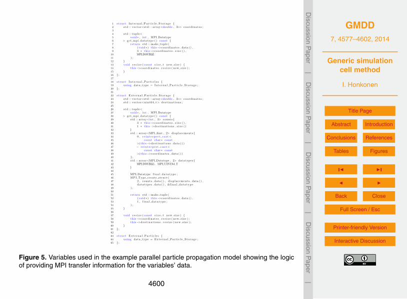
Figure 5 shows the variables used in the parallel particle propagation exampleavailable at: examples/particle_propagation/parallel/4. The particles in each cell are5

stored as a vector of arrays, i.e. the dimensionality of particle coordinates is knownat compile time but the number of particle in each cell is not. As MPI requires thatthe (maximum) amount of data to receive from another process is known in advancethe number of particles in a cell must be transferred in a separate message beforethe particles themselves. Here the number of particles is stored as a separate vari-10

able named Number_Of_Particles. The transfer of variables with complex types, forexample types whose size or memory layout changes at run time, is supported viathe get_mpi_datatype() mechanism, i.e. such types must define a get_mpi_datatype()function which provides the required transfer information to the generic cell class. Forexample in Fig. 5 the variables themselves again only define the type of the variable15

on lines 19 and 64 while the types themselves contain the logic related to MPI transferinformation. In order to be able to reliably move particles between cells on differentprocesses, i.e. without creating duplicates or loosing particles, the particle propagatoruses two collections of particles, one for particles that stay inside of the cell in whichthey are stored (lines 1..16) and another for particles which have moved outside of their20

cell (lines 22..61). The latter variable includes information about which cell a particleshave moved to.

4 Combination of three simulations

The examples of parallel models shown in Sect. 3 can all be combined into onemodel without modifying any existing code by copying and pasting the relevant parts25

4https://github.com/nasailja/gensimcell/tree/0.5/examples/particle_propagation/parallel/

4586





https://github.com/nasailja/gensimcell/tree/0.5/examples/particle_propagation/parallel/

GMDD7, 4577–4602, 2014


I. Honkonen

Title Page



Tables Figures

J I

J I

Back Close

Full Screen / Esc



Discussion

Paper

|D

iscussionP

aper|

Discussion

Paper

|D

iscussionP

aper|

from the main.cpp file of each model into a combined cpp file available at: exam-ples/combined/parallel.cpp5. This is enabled by using a separate namespace for thesolvers and variables of each submodel, as e.g. two of them use a variable with anidentical name (Velocity) and all submodels include a function named solve. All sub-models of the combined model run in the same discretized volume and with identical5

domain decomposition. This is not mandatory though as the cell id list given to eachsolver need not be identical but in this case the memory for all variables in all cellsis always allocated when using simple variables shown e.g. in Figs. 2 or 5. If sub-models always run in non-overlapping or slightly overlapping regions of the simulatedvolume, and/or with different domain decomposition, the memory required for the vari-10

ables can be allocated at run time in regions/processes where the variables are used.This can potentially be accomplished easily by wrapping the type of each variable inthe boost::optional6 type, for example.

4.1 Coupling

In the combined model shown in previous section the submodels cannot affect each15

other as they all use different variables and are thus unable to modify each other’s data.In order to couple any two or more submodels new code must be written or existingcode must be modified. The complexity of this task depends solely on the nature of thecoupling. In simple cases where the variables used by one solver are only switched tovariables of another solver, only the template parameters given to the solver have to be20

switched. The template parameters decide which variables a solver should use, i.e. theGoL solver (examples/game_of_life/parallel/gol_solve.hpp7) internally uses a templateparameter Is_Alive_T to refer to a variable which records whether a cell is alive or not

5https://github.com/nasailja/gensimcell/blob/0.5/examples/combined/parallel.cpp6http://www.boost.org/doc/libs/1_55_0/libs/optional/doc/html/index.html7https://github.com/nasailja/gensimcell/blob/0.5/examples/game_of_life/parallel/gol_solve.

hpp

4587





https://github.com/nasailja/gensimcell/blob/0.5/examples/combined/parallel.cpp

http://www.boost.org/doc/libs/1_55_0/libs/optional/doc/html/index.html

https://github.com/nasailja/gensimcell/blob/0.5/examples/game_of_life/parallel/gol_solve.hpp

https://github.com/nasailja/gensimcell/blob/0.5/examples/game_of_life/parallel/gol_solve.hpp

GMDD7, 4577–4602, 2014


I. Honkonen

Title Page



Tables Figures

J I

J I

Back Close

Full Screen / Esc



Discussion

Paper

|D

iscussionP

aper|

Discussion

Paper

|D

iscussionP

aper|

and the actual variable used for that purpose (Is_Alive) is given to the solver functionin the main program (examples/game_of_life/parallel/main.cpp8).

Figure 6 shows an example of a one way coupling of the parallel particle propagationmodel with the advection model by periodically using the velocity field of the advectionmodel in the particle propagation model. On line 6 the particle solver is called with5

the velocity field of the advection model as the velocity variable to use while on line15 the particle model’s regular velocity field is used. More complex cases of coupling,which require e.g. additional variables, are also simple to accomplish from the softwaredevelopment point of view. Additional variables can be freely inserted into the genericcell class and used by new couplers without affecting any other submodels.10

5 Effect on serial and parallel performance

In order to be usable in practice the generic cell class should not slow down a com-putational model too much. I test this using two programs: a serial GoL model anda parallel particle propagation model. The tests are conducted on a four core 2.6 GHzIntel Core i7 CPU with 256 kB L2 cache per core, 16 GB of 1600 MHz DDR3 RAM15

and the following software (installed from MacPorts where applicable): OS X 10.9.2,GCC 4.8.2_0, Open MPI 1.7.4, Boost 1.55.0_1 and dccrg commit 7d5580a30 dated12 January 2014 from the c++11 branch at https://gitorious.org/dccrg/dccrg. The testprograms are compiled with -O3 -std=c++0x.

5.1 Serial performance20

Serial performance of the generic cell is tested by playing GoL for 30 000 steps ona 100 by 100 grid with periodic boundaries and allocated at compile time. Performanceis compared against an implementation using struct { bool; int; }; as the cell

8https://github.com/nasailja/gensimcell/blob/0.5/examples/game_of_life/parallel/main.cpp

4588





https://gitorious.org/dccrg/dccrg

https://github.com/nasailja/gensimcell/blob/0.5/examples/game_of_life/parallel/main.cpp

GMDD7, 4577–4602, 2014


I. Honkonen

Title Page



Tables Figures

J I

J I

Back Close

Full Screen / Esc



Discussion

Paper

|D

iscussionP

aper|

Discussion

Paper

|D

iscussionP

aper|

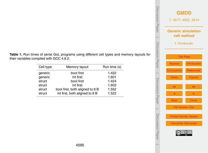
type. Both implementations are available in the directory tests/serial/game_of_life9.Each timing is obtained by executing 5 runs, discarding the slowest and fastest runsand averaging the remaining 3 runs. As shown in Table 1 serial performance is notaffected by the generic cell class, but the memory layout of variables regardless of thecell type used affects performance over 10 %. Column 2 specifies whether is_alive or5

live_neighbors is stored at a lower memory address in each cell. By default the memoryalignment of the variables is implementation defined but on the last two rows of Table 1alignas (8) is used to obtain 8 byte alignment for both variables. The order of the vari-ables in memory in a generic cell consisting of more than one variable is not definedby the standard. On the tested system the variables are laid out in memory by GCC in10

reverse order with respect to the order of the template arguments. Other compilers donot show as large differences between different ordering of variables, with ICC 14.0.2all run times are about 6 s using either -O3 or -fast (alignas is not yet supported) andwith Clang 3.4 from MacPorts all run times are about 3.5 s (about 3.6 s using alignas).

5.2 Parallel performance15

Parallel performance of the generic cell class is evaluated with a particle propagationtest which uses more complex variable types than the GoL test in order to emphasizethe computational cost of setting up MPI transfer information in the generic cell classand a manually written reference cell class. Both implementations are available in thedirectory tests/parallel/particle_propagation10. Parallel tests are run using 3 processes20

and the final time is the average of the times reported by each process. Similarly tothe serial case each test is executed 5 times, outliers are discarded and the final resultaveraged over the remaining 3 runs. The tests are run on a 203 grid without periodicboundaries and RANDOM load balancing is used to emphasize the cost of MPI trans-fers. Again there is an insignificant difference between the run times of both versions25

9https://github.com/nasailja/gensimcell/tree/0.5/tests/serial/game_of_life/10https://github.com/nasailja/gensimcell/tree/0.5/tests/parallel/particle_propagation/

4589





https://github.com/nasailja/gensimcell/tree/0.5/tests/serial/game_of_life/

https://github.com/nasailja/gensimcell/tree/0.5/tests/parallel/particle_propagation/

GMDD7, 4577–4602, 2014


I. Honkonen

Title Page



Tables Figures

J I

J I

Back Close

Full Screen / Esc



Discussion

Paper

|D

iscussionP

aper|

Discussion

Paper

|D

iscussionP

aper|

as the run time for the generic cell class version is 2.86 s while the reference imple-mentation runs in 2.92 s. The output files of the different versions are bit identical if thesame number of processes is used. When using recursive coordinate bisection loadbalancing the run times are also comparable but almost an order of magnitude lower(about 0.5 s). A similar result is expected for a larger number of processes as the bot-5

tleneck will likely be in the actual transfer of data instead of the logic for setting up thetransfers.

6 Converting existing software

Existing software can be gradually converted to use a generic cell syntax but the detailsdepend heavily on the modularity of said software and especially on the way data in10

transferred between processes. If a grid library decides what to transfer and where andthe cells provide this information via an MPI datatype, conversion will likely require onlysmall changes.

Figure 7 shows an example of converting a Conway’s Game of Life program usingcell-based storage (after Fig. 4 of Honkonen et al., 2013) to the application program-15

ming interface used by the generic cell class. In this case the underlying grid libraryhandles data transfers between processes so the only additions required are emptyclasses for denoting simulation variables and the corresponding [] operators for ac-cessing the variables’ data. With these additions the program can be converted step-by-step to use the generic cell class API and once complete the cell implementation20

shown in Fig. 7 can be swapped with the generic cell.

7 Discussion

The presented generic simulation cell method has several advantages over traditionalimplementations:

4590





GMDD7, 4577–4602, 2014


I. Honkonen

Title Page



Tables Figures

J I

J I

Back Close

Full Screen / Esc



Discussion

Paper

|D

iscussionP

aper|

Discussion

Paper

|D

iscussionP

aper|

1. The changes requred for combining and coupling models are minimal and in thepresented examples no changes to existing code are required for combining mod-els. This is advantageous for program development as submodels can be testedand verified independently and also subsequently used without modification whichdecreases the possibility of bugs and increases confidense in the correct function-5

ing of the larger program.

2. The generic simulation cell method enables zero-copy code coupling as an in-termediate representation for model variables is not necessary due to the datatypes of simulation variables being visible outside of each model. Thus if coupledmodels use a compatible representation for data, such as IEEE floating point,10

the variables of one model can be used directly by another one without the firstmodel having to export the data to an intermediate format. This again decreasesthe chance for bugs by reducing the required development effort and by allowingthe compiler to perform type checking for the entire program and warn in cases ofe.g. undefined behavior (Wang et al., 2012).15

3. Arguably code readability is also improved by making simulation variables sep-arate classes and composing models from a set of such variables. Shorthandnotation for code which resembles traditional scientific code is also possible byusing the same instance of a variable for accessing its data in cells:

const Mass_Density Rho{};20

const Background_Magnetic_Field B0{};cell_data[Rho] = ...;cell_data[B0][0] = ...;cell_data[B0][1] = ...;...25

The possibility of using a generic simulation cell approach in the traditional high-performance language of choice – Fortran – seems unlikely as Fortran currently lacks

4591





GMDD7, 4577–4602, 2014


I. Honkonen

Title Page



Tables Figures

J I

J I

Back Close

Full Screen / Esc



Discussion

Paper

|D

iscussionP

aper|

Discussion

Paper

|D

iscussionP

aper|

support for compile-time generic programming (McCormack, 2005). For example a re-cently presented computational fluid dynamics package implemented in Fortran, usingan object oriented approach and following good software development practices (Za-ghi, 2014), uses hard-coded names for variables throughout the application. Thus if thenames of any variables had to be changed for some reason, e.g. coupling to another5

model using identical variable names, all code using those variables would have to bemodified and tested to make sure no bugs have been introduced.

8 Conclusions

I present a generic simulation cell method which allows one to write generic and mod-ular computational models without sacrificing serial or parallel performance or code10

readability. I show that by using this method it is possible to combine several computa-tional models without modifying any existing code and only write new code for couplingmodels. This is a significant advantage for model development which reduces the prob-ability of bugs and eases development, testing and validation of computational models.Performance tests indicate that the effect of the presented generic simulation cell class15

on serial and parallel performance is negligible.

Acknowledgements. Alex Glocer for insightful discussions and the NASA Postdoctoral Programfor financial support.

References

Du Toit, S.: Working Draft, Standard for Programming Language C++, ISO/IEC, avail-20

able at: http://www.open-std.org/jtc1/sc22/wg21/docs/papers/2012/n3337.pdf (last access:15 July 2014), 2012. 4581

Eller, P., Singh, K., Sandu, A., Bowman, K., Henze, D. K., and Lee, M.: Implementation andevaluation of an array of chemical solvers in the Global Chemical Transport Model GEOS-Chem, Geosci. Model Dev., 2, 89–96, doi:10.5194/gmd-2-89-2009, 2009. 458125

4592





http://www.open-std.org/jtc1/sc22/wg21/docs/papers/2012/n3337.pdf

http://dx.doi.org/10.5194/gmd-2-89-2009

GMDD7, 4577–4602, 2014


I. Honkonen

Title Page



Tables Figures

J I

J I

Back Close

Full Screen / Esc



Discussion

Paper

|D

iscussionP

aper|

Discussion

Paper

|D

iscussionP

aper|

Hill, C., DeLuca, C., Balaji, V., Suarez, M., and Silva, A. D.: The architecture of the earth systemmodeling framework, Comp. Sci. Eng., 6, 18–28, doi:10.1109/MCISE.2004.1255817, 2004.4580

Honkonen, I., von Alfthan, S., Sandroos, A., Janhunen, P., and Palmroth, M.: Parallel grid li-brary for rapid and flexible simulation development, Comp. Phys. Commun., 184, 1297–1309,5

doi:10.1016/j.cpc.2012.12.017, 2013. 4583, 4584, 4585, 4590, 4599, 4602Jöckel, P., Sander, R., Kerkweg, A., Tost, H., and Lelieveld, J.: Technical Note: The Modular

Earth Submodel System (MESSy) - a new approach towards Earth System Modeling, Atmos.Chem. Phys., 5, 433–444, doi:10.5194/acp-5-433-2005, 2005. 4580

Larson, J., Jacob, R., and Ong, E.: The model coupling toolkit: a new Fortran90 toolkit10

for building multiphysics parallel coupled models, Int. J. High Perform. C., 19, 277–292,doi:10.1177/1094342005056115, 2005. 4580

McCormack, D.: Generic programming in Fortran with Forpedo, SIGPLAN Fortran Forum, 24,18–29, doi:10.1145/1080399.1080401, 2005. 4592

Miller, G.: A scientist’s nightmare: software problem leads to five retractions, Science, 314,15

1856–1857, doi:10.1126/science.314.5807.1856, 2006. 4579Musser, D. R. and Stepanov, A. A.: Generic programming, in: Symbolic and Algebraic Compu-

tation, edited by: Gianni, P., vol. 358 of Lecture Notes in Computer Science, Springer, Berlin,Heidelberg, doi:10.1007/3-540-51084-2_2, 13–25, available at: http://www.stepanovpapers.com/genprog.ps, 1989. 457920

Oberkampf, W. L. and Trucano, T. G.: Verification and validation in computational fluid dynam-ics, Prog. Aerosp. Sci., 38, 209–272, doi:10.1016/S0376-0421(02)00005-2, 2002. 4579

Post, D. E. and Votta, L. G.: Computational science demands a new paradigm, Phys. Today,58, 35–41, doi:10.1063/1.1881898, 2005. 4578

Redler, R., Valcke, S., and Ritzdorf, H.: OASIS4 – a coupling software for next generation earth25

system modelling, Geosci. Model Dev., 3, 87–104, doi:10.5194/gmd-3-87-2010, 2010. 4580Stroustrup, B.: Learning standard C++ as a new language, C/C++ Users J., 17, 43–54, avail-

able at: http://dl.acm.org/citation.cfm?id=315554.315565, 1999. 4579Thomas, W. M., Delis, A., and Basili, V. R.: An analysis of errors in a reuse-oriented devel-

opment environment, J. Syst. Software, 38, 211–224, doi:10.1016/S0164-1212(96)00152-5,30

1997. 4579Toth, G., Sokolov, I. V., Gombosi, T. I., Chesney, D. R., Clauer, C. R., De Zeeuw, D. L.,

Hansen, K. C., Kane, K. J., Manchester, W. B., Oehmke, R. C., Powell, K. G., Ridley, A. J.,

4593





http://dx.doi.org/10.1109/MCISE.2004.1255817

http://dx.doi.org/10.1016/j.cpc.2012.12.017

http://dx.doi.org/10.5194/acp-5-433-2005

http://dx.doi.org/10.1177/1094342005056115

http://dx.doi.org/10.1145/1080399.1080401

http://dx.doi.org/10.1126/science.314.5807.1856

http://dx.doi.org/10.1007/3-540-51084-2_2

http://www.stepanovpapers.com/genprog.ps



http://dx.doi.org/10.1016/S0376-0421(02)00005-2

http://dx.doi.org/10.1063/1.1881898

http://dx.doi.org/10.5194/gmd-3-87-2010

http://dl.acm.org/citation.cfm?id=315554.315565

http://dx.doi.org/10.1016/S0164-1212(96)00152-5

GMDD7, 4577–4602, 2014


I. Honkonen

Title Page



Tables Figures

J I

J I

Back Close

Full Screen / Esc



Discussion

Paper

|D

iscussionP

aper|

Discussion

Paper

|D

iscussionP

aper|

Roussev, I. I., Stout, Q. F., Volberg, O., Wolf, R. A., Sazykin, S., Chan, A., Yu, B., and Kota, J.:Space weather modeling framework: a new tool for the space science community, J. Geo-phys. Res.-Space, 110, A12226, doi:10.1029/2005JA011126, 2005. 4580

Waligora, S., Bailey, J., and Stark, M.: Impact Of Ada And Object-Oriented Design In The FlightDynamics Division At Goddard Space Flight Center, Tech. rep., National Aeronautics and5

Space Administration, Goddard Space Flight Center, 1995. 4579Wang, X., Chen, H., Cheung, A., Jia, Z., Zeldovich, N., and Kaashoek, M. F.: Undefined behav-

ior: what happened to my code?, in: Proceedings of the Asia-Pacific Workshop on Systems,APSYS ’12, ACM, New York, NY, USA, 9:1–9:7, doi:10.1145/2349896.2349905, 2012. 4591

Zaghi, S.: OFF, Open source Finite volume Fluid dynamics code: a free, high-order solver10

based on parallel, modular, object-oriented Fortran {API}, Comput. Phys. Commun., 185,2151–2194, doi:10.1016/j.cpc.2014.04.005, 2014. 4592

Zhang, L. and Parashar, M.: Seine: a dynamic geometry-based shared space interaction frame-work for parallel scientific applications, in: Proceedings of High Performance Computing –HiPC 2004: 11th International Conference, Springer LNCS, 189–199, 2006. 4580

4594





http://dx.doi.org/10.1029/2005JA011126

http://dx.doi.org/10.1145/2349896.2349905

http://dx.doi.org/10.1016/j.cpc.2014.04.005

GMDD7, 4577–4602, 2014


I. Honkonen

Title Page



Tables Figures

J I

J I

Back Close

Full Screen / Esc



Discussion

Paper

|D

iscussionP

aper|

Discussion

Paper

|D

iscussionP

aper|

Table 1. Run times of serial GoL programs using different cell types and memory layouts fortheir variables compiled with GCC 4.8.2.

Cell type Memory layout Run time (s)

generic bool first 1.422generic int first 1.601struct bool first 1.424struct int first 1.603struct bool first, both aligned to 8 B 1.552struct int first, both aligned to 8 B 1.522

4595





GMDD7, 4577–4602, 2014


I. Honkonen

Title Page



Tables Figures

J I

J I

Back Close

Full Screen / Esc



Discussion

Paper

|D

iscussionP

aper|

Discussion

Paper

|D

iscussionP

aper|

Honkonen: Generic simulation cell method 3

rest of the text refer to the version of the generic simula-tion cell tagged as 0.5 in the git repository and is available at:175

https://github.com/nasailja/gensimcell/tree/0.5/.

2 Serial implementation

Figure 1 shows a basic implementation of the generic simula-tion cell class that does not provide support for MPI applica-tions and is not const-correct but is otherwise complete. The180

cell class takes as input an arbitrary number of template pa-rameters that correspond to variables to be stored in the cell.Each varible only defines its type through the name data_type(e.g. lines 5 and 6 in Figure 2) and is otherwise empty. Whenthe cell class is given one variable as a template argument185

the code on lines 3..13 is used. The variable given to the cellclass as a template parameter is stored as a private memberof the cell class on line 5 and access to it is provided by thecell’s [] operator overloaded for the variable’s class on lines8..12. When given multiple variables as template arguments190

the code on lines 15..33 is used which similarly stores thefirst variable as a private member and provides access to itvia the [] operator. Additionally the cell class derives fromfrom itself with one less variable on line 21. This recursionis stopped by eventually inheriting the one variable version of195

the cell class. Access to the private data members represent-ing all variables are provided by the respective [] operatorswhich are made available to outside of the cell class on line26. The memory layout of variables in an instance of the cellclass depends on the compiler implementation and can in-200

clude, for example, padding between variables given as con-secutive template parameters. This also applies to variablesstored in "ordinary" structures and in both cases if, for exam-ple, several values must be stored contiguously in memory acontainer guaranteeing this should be used such as std::array205

or std::vector.Figure 2 shows a complete serial implementation of Con-

way’s Game of Life (GoL) using the generic simulation cellclass. A version of this example with console output is avail-able at examples/game_of_life/serial.cpp1. Lines 5..7 define210

the variables to be used in the model and the cell type tobe used in the model grid. Lines 10..20 create the simulationgrid and initialize the simulation with a pseudorandom initialcondition. The time stepping loop spans lines 22..57. The []operator is used to obtain a reference to the data of all vari-215

ables e.g. on lines 17 and 42. Lines 26 and 34 provide a shorthand name for the curret cell and its neighbors respectively.Using the generic cell class adds hardly any code comparedto a traditional implementation (e.g. Figure 4 in Honkonenet al., 2013) and allows the types of the variables used in the220

model to be defined outside of both the grid which stores thesimulation variables and the solver functions which use thevariables to calculate the solution.

1https://github.com/nasailja/gensimcell/blob/0.5/examples/game_of_life/serial.cpp

1 template <c l a s s . . . Var iab les> c l a s s Ce l l ;2

3 template <c l a s s Variable> c l a s s Cel l<Variable> {4 pr i va t e :5 typename Var iab le : : data type data ;6

7 pub l i c :8 typename Var iab le : : data type& operator [ ] (9 const Var iab le&

10 ) {11 re turn th i s−>data ;12 }13 } ;14

15 template <16 c l a s s Current Var iab le ,17 c l a s s . . . Res t Of Var iab l e s18 > c l a s s Cel l<19 Current Var iab le ,20 Rest Of Var iab l e s . . .21 > : pub l i c Cel l<Rest Of Var iab l e s . . . > {22 pr i va t e :23 typename Current Var iab le : : data type data ;24

25 pub l i c :26 us ing Cel l<Rest Of Var iab l e s . . . > : : operator [ ] ;27

28 typename Current Var iab le : : data type& operator [ ] (29 const Current Var iab le&30 ) {31 re turn th i s−>data ;32 }33 } ;

Fig. 1. Serial implementation of the generic simulation cell classthat is not const-correct but is otherwise complete.

Figure 3 shows excerpts from serial versions ofprograms modeling advection and particle propagation225

in prescribed velocity fields. The full examples areavailable at examples/advection/serial.cpp2 and exam-ples/particle_propagation/serial.cpp3. The variables of bothmodels are defined similarly to Figure 2 and the [] operatoris used to refer to the variables’ data in each cell.230

3 Parallel implementation

In a parallel computational model variables in neighboringcells must be transferred between processes in order to cal-culate the solution at the next time step or iteration. On theother hand it might not be necessary to transfer all variables235

in each communication as one solver could be using higherorder time stepping than others and require more iterationsfor each time step. Or, for example, when modeling an in-compressible fluid the Poisson’s equation for pressure mustbe solved at each time step, i.e. iterated in parallel until some240

norm of the residual becomes small enough, during which

2https://github.com/nasailja/gensimcell/blob/0.5/examples/advection/serial.cpp

3https://github.com/nasailja/gensimcell/blob/0.5/examples/particle_propagation/serial.cpp

Figure 1. Serial implementation of the generic simulation cell class that is not const-correct butis otherwise complete.

4596





GMDD7, 4577–4602, 2014


I. Honkonen

Title Page



Tables Figures

J I

J I

Back Close

Full Screen / Esc



Discussion

Paper

|D

iscussionP

aper|

Discussion

Paper

|D

iscussionP

aper|

4 Honkonen: Generic simulation cell method

1 #inc lude ” array ”2 #inc lude ” c s t d l i b ”3 #inc lude ” g en s imce l l . hpp”4

5 s t r u c t I s A l i v e { us ing data type = bool ; } ;6 s t r u c t Live Neighbors { us ing data type = in t ; } ;7 us ing Cel l T = gen s imce l l : : Ce l l<I s A l i v e , Live Neighbors >;8

9 i n t main ( ) {10 constexpr s i z e t width = 10 , he ight = 10 ;11 std : : array<std : : array<Cell T , width>, he ight> g r id ;12 // i n i t i a l c ond i t i on13 f o r ( auto& row : g r id ) {14 f o r ( auto& c e l l : row ) {15 c e l l [ L ive Neighbors ( ) ] = 0 ;16 i f ( rand ( ) < RANDMAX / 10)17 c e l l [ I s A l i v e ( ) ] = true ;18 e l s e19 c e l l [ I s A l i v e ( ) ] = f a l s e ;20 }}21

22 f o r ( i n t s tep = 0 ; s tep < 20 ; s tep++) {23 // c o l l e c t l i v e ne ighbor counts24 f o r ( s i z e t row = 0 ; row < he ight ; row++) {25 f o r ( s i z e t c o l = 0 ; c o l < width ; c o l++) {26 auto& c e l l = gr id [ row ] [ c o l ] ;27

28 // neighbor index o f f s e t s : +1, 0 , −129 f o r ( auto r ow o f f s e t : {1ul , 0ul , width − 1}) {30 f o r ( auto c o l o f f s e t : {1ul , 0ul , he ight − 1}) {31 i f ( r ow o f f s e t == 0 and c o l o f f s e t == 0)32 cont inue ;33 // p e r i o d i c boundar ies34 const auto& neighbor35 = gr id [36 ( row + row o f f s e t ) % he ight37 ] [38 ( c o l + c o l o f f s e t ) % width39 ] ;40

41 i f ( ne ighbor [ I s A l i v e ( ) ] )42 c e l l [ L ive Neighbors ()]++;43 }}44 }}45 // s e t new s t a t e46 f o r ( s i z e t row = 0 ; row < he ight ; row++) {47 f o r ( s i z e t c o l = 0 ; c o l < width ; c o l++) {48 Cel l T& c e l l = gr id [ row ] [ c o l ] ;49

50 i f ( c e l l [ L ive Ne ighbors ( ) ] == 3)51 c e l l [ I s A l i v e ( ) ] = true ;52 e l s e i f ( c e l l [ L ive Neighbors ( ) ] != 2)53 c e l l [ I s A l i v e ( ) ] = f a l s e ;54

55 c e l l [ L ive Neighbors ( ) ] = 0 ;56 }}57 }58 re turn 0 ;59 }

Fig. 2. A serial program playing Conway’s Game of Life imple-mented using the generic simulation cell class.

time other variables need not be transferred. Several modelvariables can also be used for debugging and need not alwaysbe transferred between processes.

The generic cell class provides support for parallel pro-245

grams via a get_mpi_datatype() member function which canbe used to query what data should be transferred to/froma generic cell with MPI. The transfer of one or more vari-ables can be switched on or off via a function overloaded foreach variable on a cell-by-cell basis. This allows the com-250

munication strategy of a program to be formalized by ex-plicitly stating which variables must be transferred between

1 /∗ advect ion ∗/2 s t r u c t Density { us ing data type = double ; } ;3 s t r u c t Dens ity Flux { us ing data type = double ; } ;4 s t r u c t Ve loc i ty { us ing data type = std : : array<double , 2>; } ;5 us ing Cel l T = gen s imce l l : : Ce l l<Density , Density Flux , Ve loc i ty >;6 us ing Grid T = array<array<Cell T , width>, he ight >;7

8 void app l y s o l u t i on (Grid T& gr id ) {9 f o r ( auto& row : g r id ) {

10 f o r ( auto& c e l l : row ) {11 c e l l [ Density ( ) ] += c e l l [ Dens i ty Flux ( ) ] ;12 c e l l [ Dens i ty Flux ( ) ] = 0 ;13 }}14 }15

16 /∗ p a r t i c l e propagat ion ∗/17 s t r u c t Ve loc i ty { us ing data type = array<double , 2>; } ;18 s t r u c t P a r t i c l e s { us ing data type = vector<array<double , 2>>; } ;19 us ing Cel l T = gen s imce l l : : Ce l l<Veloc i ty , Pa r t i c l e s> Cel l T ;20 us ing Grid T = array<array<Cell T , width>, he ight >;21

22 void i n i t i a l i z e ( Grid T& gr id ) {23 f o r ( s i z e t row i = 0 ; row i < he ight ; row i++) {24 f o r ( s i z e t c e l l i = 0 ; c e l l i < width ; c e l l i ++) {25

26 const auto27 c e l l c e n t e r = g e t c e l l c e n t e r ( gr id , { c e l l i , row i } ) ,28 c e l l s i z e = g e t c e l l s i z e ( gr id , { c e l l i , row i } ) ;29

30 auto& c e l l = gr id [ row i ] [ c e l l i ] ;31

32 c e l l [ P a r t i c l e s ( ) ] . push back ({33 c e l l c e n t e r [ 0 ] − c e l l s i z e [ 0 ] / 4 ,34 c e l l c e n t e r [ 1 ] − c e l l s i z e [ 1 ] / 435 } ) ;36 }}37 }

Fig. 3. Excerpts from separate serial programs using the genericsimulation cell class modeling advection and particle propagationin a prescribed velocity field.

processes for the correct functionality of each solver andthe entire program. The parallel code presented here is builton top of the dccrg library Honkonen et al. (2013) which255

handles the details of e.g. transferring the data of neighbor-ing simulation cells accross process boundaries by callingthe get_mpi_datatype() member function of each cell whenneeded.

Standard types whose size is known at compile-time (e.g.260

int, float, std::array<int, N>, but see Section 3 for the gen-eral case) can be transferred without extra code from theuser. Functions are provided by the cell class for switchingon or off the transfer of one or more variables in all in-stances of a particular type of cell (set_transfer_all()) and265

for switching on or off the transfers in each instance sep-arately (set_transfer()). The former function takes as argu-ments a boost::tribool value and the affected variables. Ifthe triboolean value is determined (true of false) then allinstances behave identically for the affected variables, oth-270

erwise (indeterminate) the decision to transfer the affectedvariables is controlled on a cell-by-cell basis by the latterfunction. The functions are implemented recursively usingvariadic templates in order to allow the user to switch on/offthe transfer of arbitrary combinations of variables in the same275

function call. When the cell class returns the MPI transfer in-formation via its get_mpi_datatype() member function, all

Figure 2. A serial program playing Conway’s Game of Life implemented using the genericsimulation cell class.

4597





GMDD7, 4577–4602, 2014


I. Honkonen

Title Page



Tables Figures

J I

J I

Back Close

Full Screen / Esc



Discussion

Paper

|D

iscussionP

aper|

Discussion

Paper

|D

iscussionP

aper|


1 #inc lude ” array ”2 #inc lude ” c s t d l i b ”3 #inc lude ” g en s imce l l . hpp”4

5 s t r u c t I s A l i v e { us ing data type = bool ; } ;6 s t r u c t Live Neighbors { us ing data type = in t ; } ;7 us ing Cel l T = gen s imce l l : : Ce l l<I s A l i v e , Live Neighbors >;8

9 i n t main ( ) {10 constexpr s i z e t width = 10 , he ight = 10 ;11 std : : array<std : : array<Cell T , width>, he ight> g r id ;12 // i n i t i a l c ond i t i on13 f o r ( auto& row : g r id ) {14 f o r ( auto& c e l l : row ) {15 c e l l [ L ive Neighbors ( ) ] = 0 ;16 i f ( rand ( ) < RANDMAX / 10)17 c e l l [ I s A l i v e ( ) ] = true ;18 e l s e19 c e l l [ I s A l i v e ( ) ] = f a l s e ;20 }}21

22 f o r ( i n t s tep = 0 ; s tep < 20 ; s tep++) {23 // c o l l e c t l i v e ne ighbor counts24 f o r ( s i z e t row = 0 ; row < he ight ; row++) {25 f o r ( s i z e t c o l = 0 ; c o l < width ; c o l++) {26 auto& c e l l = gr id [ row ] [ c o l ] ;27

28 // neighbor index o f f s e t s : +1, 0 , −129 f o r ( auto r ow o f f s e t : {1ul , 0ul , width − 1}) {30 f o r ( auto c o l o f f s e t : {1ul , 0ul , he ight − 1}) {31 i f ( r ow o f f s e t == 0 and c o l o f f s e t == 0)32 cont inue ;33 // p e r i o d i c boundar ies34 const auto& neighbor35 = gr id [36 ( row + row o f f s e t ) % he ight37 ] [38 ( c o l + c o l o f f s e t ) % width39 ] ;40

41 i f ( ne ighbor [ I s A l i v e ( ) ] )42 c e l l [ L ive Neighbors ()]++;43 }}44 }}45 // s e t new s t a t e46 f o r ( s i z e t row = 0 ; row < he ight ; row++) {47 f o r ( s i z e t c o l = 0 ; c o l < width ; c o l++) {48 Cel l T& c e l l = gr id [ row ] [ c o l ] ;49

50 i f ( c e l l [ L ive Ne ighbors ( ) ] == 3)51 c e l l [ I s A l i v e ( ) ] = true ;52 e l s e i f ( c e l l [ L ive Neighbors ( ) ] != 2)53 c e l l [ I s A l i v e ( ) ] = f a l s e ;54

55 c e l l [ L ive Neighbors ( ) ] = 0 ;56 }}57 }58 re turn 0 ;59 }

Fig. 2. A serial program playing Conway’s Game of Life imple-mented using the generic simulation cell class.

time other variables need not be transferred. Several modelvariables can also be used for debugging and need not alwaysbe transferred between processes.

The generic cell class provides support for parallel pro-245

grams via a get_mpi_datatype() member function which canbe used to query what data should be transferred to/froma generic cell with MPI. The transfer of one or more vari-ables can be switched on or off via a function overloaded foreach variable on a cell-by-cell basis. This allows the com-250

munication strategy of a program to be formalized by ex-plicitly stating which variables must be transferred between

1 /∗ advect ion ∗/2 s t r u c t Density { us ing data type = double ; } ;3 s t r u c t Dens ity Flux { us ing data type = double ; } ;4 s t r u c t Ve loc i ty { us ing data type = std : : array<double , 2>; } ;5 us ing Cel l T = gen s imce l l : : Ce l l<Density , Density Flux , Ve loc i ty >;6 us ing Grid T = array<array<Cell T , width>, he ight >;7

8 void app l y s o l u t i on (Grid T& gr id ) {9 f o r ( auto& row : g r id ) {

10 f o r ( auto& c e l l : row ) {11 c e l l [ Density ( ) ] += c e l l [ Dens i ty Flux ( ) ] ;12 c e l l [ Dens i ty Flux ( ) ] = 0 ;13 }}14 }15

16 /∗ p a r t i c l e propagat ion ∗/17 s t r u c t Ve loc i ty { us ing data type = array<double , 2>; } ;18 s t r u c t P a r t i c l e s { us ing data type = vector<array<double , 2>>; } ;19 us ing Cel l T = gen s imce l l : : Ce l l<Veloc i ty , Pa r t i c l e s> Cel l T ;20 us ing Grid T = array<array<Cell T , width>, he ight >;21

22 void i n i t i a l i z e ( Grid T& gr id ) {23 f o r ( s i z e t row i = 0 ; row i < he ight ; row i++) {24 f o r ( s i z e t c e l l i = 0 ; c e l l i < width ; c e l l i ++) {25

26 const auto27 c e l l c e n t e r = g e t c e l l c e n t e r ( gr id , { c e l l i , row i } ) ,28 c e l l s i z e = g e t c e l l s i z e ( gr id , { c e l l i , row i } ) ;29

30 auto& c e l l = gr id [ row i ] [ c e l l i ] ;31

32 c e l l [ P a r t i c l e s ( ) ] . push back ({33 c e l l c e n t e r [ 0 ] − c e l l s i z e [ 0 ] / 4 ,34 c e l l c e n t e r [ 1 ] − c e l l s i z e [ 1 ] / 435 } ) ;36 }}37 }

Fig. 3. Excerpts from separate serial programs using the genericsimulation cell class modeling advection and particle propagationin a prescribed velocity field.

processes for the correct functionality of each solver andthe entire program. The parallel code presented here is builton top of the dccrg library Honkonen et al. (2013) which255

handles the details of e.g. transferring the data of neighbor-ing simulation cells accross process boundaries by callingthe get_mpi_datatype() member function of each cell whenneeded.

Standard types whose size is known at compile-time (e.g.260

int, float, std::array<int, N>, but see Section 3 for the gen-eral case) can be transferred without extra code from theuser. Functions are provided by the cell class for switchingon or off the transfer of one or more variables in all in-stances of a particular type of cell (set_transfer_all()) and265

for switching on or off the transfers in each instance sep-arately (set_transfer()). The former function takes as argu-ments a boost::tribool value and the affected variables. Ifthe triboolean value is determined (true of false) then allinstances behave identically for the affected variables, oth-270

erwise (indeterminate) the decision to transfer the affectedvariables is controlled on a cell-by-cell basis by the latterfunction. The functions are implemented recursively usingvariadic templates in order to allow the user to switch on/offthe transfer of arbitrary combinations of variables in the same275

function call. When the cell class returns the MPI transfer in-formation via its get_mpi_datatype() member function, all

Figure 3. Excerpts from separate serial programs using the generic simulation cell class mod-eling advection and particle propagation in a prescribed velocity field.

4598





GMDD7, 4577–4602, 2014


I. Honkonen

Title Page



Tables Figures

J I

J I

Back Close

Full Screen / Esc



Discussion

Paper

|D

iscussionP

aper|

Discussion

Paper

|D

iscussionP

aper|


1 . . .2 #inc lude ” dccrg . hpp”3 #inc lude ” dcc rg ca r t e s i an geomet ry . hpp”4 #inc lude ” g en s imce l l . hpp”5 . . .6 i n t main ( i n t argc , char ∗ argv [ ] ) {7 us ing Ce l l = go l : : Ce l l ;8 i f ( MPI Init(&argc , &argv ) != MPI SUCCESS) { . . . }9

10 dccrg : : Dccrg<Cel l , dccrg : : Cartesian Geometry> g r id ;11 . . .12 go l : : i n i t i a l i z e <Cel l , go l : : I s A l i v e , go l : : L ive Neighbors >( g r id ) ;13

14 const std : : vector<u int64 t>15 i n n e r c e l l s = gr id . g e t l o c a l c e l l s n o t o n p r o c e s s b o unda r y ( ) ,16 o u t e r c e l l s = gr id . g e t l o c a l c e l l s o n p r o c e s s b o und a r y ( ) ;17 . . .18 whi le ( s imu la t i on t ime <= M PI) {19 . . .20 Ce l l : : s e t t r a n s f e r a l l ( true , go l : : I s A l i v e ( ) ) ;21 g r id . s t a r t r emote ne i ghbor copy update s ( ) ;22 go l : : so lve<23 Cel l ,24 go l : : I s A l i v e ,25 go l : : L ive Neighbors26 >( i n n e r c e l l s , g r i d ) ;27 g r id . wa i t r emote ne i ghbo r copy updat e r e c e i v e s ( ) ;28 go l : : so lve < . . .>( o u t e r c e l l s , g r i d ) ;29 go l : : app ly so lu t i on < . . .>( i n n e r c e l l s , g r i d ) ;30 g r id . wa i t r emote ne ighbor copy update sends ( ) ;31 go l : : app ly so lu t i on < . . .>( o u t e r c e l l s , g r i d ) ;32 s imu la t i on t ime += t ime s t ep ;33 }34 MPI Final ize ( ) ;35 re turn EXIT SUCCESS ;36 }

Fig. 4. Excerpts from a parallel program playing Conway’s Gameof Life implemented using the generic simulation cell class and thedccrg grid library (Honkonen et al., 2013).

variables are iterated through at compile-time and only thosethat should be transferred are added at run-time to the finalMPI_Datatype returned by the function.280

Figure 4 shows excerpts from the parallel version of theGoL example implemented using the generic simulation cellclass and the dccrg grid library. The cell type used by thisversion (line 7) is identical to the type used in the serial ver-sion on line 7 of Figure 2. In the parallel version the for285

loops over cells and their neighbors inside the time steppingloop have been moved to separate functions called solve andapply_solution respectively. At each time step, before start-ing cell data transfers between processes at process bound-aries (line 21), the transfer of required variables, in this case290

whether the cell is alive or not, is switched on in all cells (line20). No additional code is required for the transfer logic incontrast to a program not using the generic cell class (Honko-nen et al., 2013, e.g. lines 12 and 13 in Figure 4 of). The func-tion solving the system for a given list of cells (called solve295

in the namespace gol), which in this case counts the numberof life neighbors, is called on lines 22..26 with the cell classand variables to use internally given as template parameters.This makes the function accept cells consisting of arbitraryvariables and also allows one to change the variables used by300

the function easily.The strategy used in Figure 4 for overlapping computa-

tion and communication is also used in the other parallel ex-amples. After starting data transfers between the outer cells

of different processes the solution is calculated in the inner305

cells. Inner cells are defined as cells that do not consider cellson other processes as neighbors and that are not consideredas neighbors of cells on other processes. Outer cells are de-fined as cells other than the inner cells of a process. Once thedata of other processes’ outer cells has arrived the solution310

is calculated in local outer cells. After this the solution canbe applied to inner cells and when the data of outer cells hasarrived to other processes the solution can also be applied tothe outer cells.

Figure 5 shows the variables used in the paral-315

lel particle propagation example available at exam-ples/particle_propagation/parallel/4. The particles in eachcell are stored as a vector of arrays, i.e. the dimensional-ity of particle coordinates is known at compile time but thenumber of particle in each cell is not. As MPI requires that320

the (maximum) amount of data to receive from another pro-cess is known in advance the number of particles in a cellmust be transferred in a separate message before the particlesthemselves. Here the number of particles is stored as a sep-arate variable named Number_Of_Particles. The transfer of325

variables with complex types, for example types whose sizeor memory layout changes at run time, is supported via theget_mpi_datatype() mechanism, i.e. such types must definea get_mpi_datatype() function which provides the requiredtransfer information to the generic cell class. For example in330

Figure 5 the variables themselves again only define the typeof the variable on lines 19 and 64 while the types themselvescontain the logic related to MPI transfer information. In orderto be able to reliably move particles between cells on differ-ent processes, i.e. without creating duplicates or loosing par-335

ticles, the particle propagator uses two collections of parti-cles, one for particles that stay inside of the cell in which theyare stored (lines 1..16) and another for particles which havemoved outside of their cell (lines 22..61). The latter variableincludes information about which cell a particles have moved340

to.

4 Combination of three simulations

The examples of parallel models shown in Section 3 can allbe combined into one model without modifying any exist-ing code by copying and pasting the relevant parts from the345

main.cpp file of each model into a combined cpp file avail-able at examples/combined/parallel.cpp5. This is enabled byusing a separate namespace for the solvers and variables ofeach submodel, as e.g. two of them use a variable with anidentical name (Velocity) and all submodels include a func-350

tion named solve. All submodels of the combined model runin the same discretized volume and with identical domain

4https://github.com/nasailja/gensimcell/tree/0.5/examples/particle_propagation/parallel/

5https://github.com/nasailja/gensimcell/blob/0.5/examples/combined/parallel.cpp

Figure 4. Excerpts from a parallel program playing Conway’s Game of Life implemented usingthe generic simulation cell class and the dccrg grid library (Honkonen et al., 2013).

4599





GMDD7, 4577–4602, 2014


I. Honkonen

Title Page



Tables Figures

J I

J I

Back Close

Full Screen / Esc



Discussion

Paper

|D

iscussionP

aper|

Discussion

Paper

|D

iscussionP

aper|


1 s t r u c t I n t e r n a l P a r t i c l e S t o r a g e {2 std : : vector<std : : array<double , 3>> coo rd ina t e s ;3

4 std : : tuple<5 void ∗ , int , MPI Datatype6 > get mpi datatype ( ) const {7 re turn std : : make tuple (8 ( void ∗) th i s−>coo rd ina t e s . data ( ) ,9 3 ∗ th i s−>coo rd ina t e s . s i z e ( ) ,

10 MPI DOUBLE11 ) ;12 }13 void r e s i z e ( const s i z e t new s i z e ) {14 th i s−>coo rd ina t e s . r e s i z e ( new s i z e ) ;15 }16 } ;17

18 s t r u c t I n t e r n a l P a r t i c l e s {19 us ing data type = I n t e r n a l P a r t i c l e S t o r a g e ;20 } ;21

22 s t r u c t Ex t e r na l Pa r t i c l e S t o r a g e {23 std : : vector<std : : array<double , 3>> coo rd ina t e s ;24 std : : vector<u int64 t> d e s t i n a t i o n s ;25

26 std : : tuple<27 void ∗ , int , MPI Datatype28 > get mpi datatype ( ) const {29 std : : array<int , 2> counts {30 3 ∗ th i s−>coo rd ina t e s . s i z e ( ) ,31 1 ∗ th i s−>d e s t i n a t i o n s . s i z e ( )32 }33 std : : array<MPI Aint , 2> di sp lacements {34 0 , r e i n t e r p r e t c a s t<35 const char ∗ const36 >( th i s−>d e s t i n a t i o n s . data ( ) )37 − r e i n t e r p r e t c a s t<38 const char ∗ const39 >( th i s−>coo rd ina t e s . data ( ) )40 } ;41 std : : array<MPI Datatype , 2> datatypes {42 MPI DOUBLE, MPI UINT64 T43 }44

45 MPI Datatype f i n a l d a t a t yp e ;46 MPI Type create struct (47 2 , counts . data ( ) , d i sp lacements . data ( ) ,48 datatypes . data ( ) , &f i n a l d a t a t yp e49 ) ;50

51 re turn std : : make tuple (52 ( void ∗) th i s−>coo rd ina t e s . data ( ) ,53 1 , f i n a l d a t a t yp e ;54 ) ;55 }56

57 void r e s i z e ( const s i z e t new s i z e ) {58 th i s−>coo rd ina t e s . r e s i z e ( new s i z e ) ;59 th i s−>d e s t i n a t i o n s . r e s i z e ( new s i z e ) ;60 }61 } ;62

63 s t r u c t Ex t e r n a l Pa r t i c l e s {64 us ing data type = Ext e rna l Pa r t i c l e S t o r a g e ;65 } ;

Fig. 5. Variables used in the example parallel particle propagationmodel showing the logic of providing MPI transfer information forthe variables’ data.

decomposition. This is not mandatory though as the cell idlist given to each solver need not be identical but in this casethe memory for all variables in all cells is always allocated355

when using simple variables shown e.g. in Figures 2 or 5. Ifsubmodels always run in non-overlapping or slightly over-lapping regions of the simulated volume, and/or with dif-ferent domain decomposition, the memory required for thevariables can be allocated at run time in regions/processes360

where the variables are used. This can potentially be accom-plished easily by wrapping the type of each variable in theboost::optional6 type, for example.

4.1 Coupling

In the combined model shown in previous section the sub-365

models cannot affect each other as they all use differ-ent variables and are thus unable to modify each other’sdata. In order to couple any two or more submodels newcode must be written or existing code must be modified.The complexity of this task depends solely on the na-370

ture of the coupling. In simple cases where the variablesused by one solver are only switched to variables of an-other solver, only the template parameters given to thesolver have to be switched. The template parameters de-cide which variables a solver should use, i.e. the GoL375

solver (examples/game_of_life/parallel/gol_solve.hpp7) in-ternally uses a template parameter Is_Alive_T to refer toa variable which records whether a cell is alive or notand the actual variable used for that purpose (Is_Alive) isgiven to the solver function in the main program (exam-380

ples/game_of_life/parallel/main.cpp8).Figure 6 shows an example of a one way coupling of

the parallel particle propagation model with the advectionmodel by periodically using the velocity field of the advec-tion model in the particle propagation model. On line 6 the385

particle solver is called with the velocity field of the advec-tion model as the velocity variable to use while on line 15 theparticle model’s regular velocity field is used. More complexcases of coupling, which require e.g. additional variables, arealso simple to accomplish from the software development390

point of view. Additional variables can be freely inserted intothe generic cell class and used by new couplers without af-fecting any other submodels.

5 Effect on serial and parallel performance

In order to be usable in practice the generic cell class should395

not slow down a computational model too much. I test this

6http://www.boost.org/doc/libs/1_55_0/libs/optional/doc/html/index.html

7https://github.com/nasailja/gensimcell/blob/0.5/examples/game_of_life/parallel/gol_solve.hpp

8https://github.com/nasailja/gensimcell/blob/0.5/examples/game_of_life/parallel/main.cpp

Figure 5. Variables used in the example parallel particle propagation model showing the logicof providing MPI transfer information for the variables’ data.

4600





GMDD7, 4577–4602, 2014


I. Honkonen

Title Page



Tables Figures

J I

J I

Back Close

Full Screen / Esc



Discussion

Paper

|D

iscussionP

aper|

Discussion

Paper

|D

iscussionP

aper|


1 i f ( s td : : fmod ( s imulat ion t ime , 1) < 0 . 5 ) {2 p a r t i c l e : : so lve<3 Cel l ,4 p a r t i c l e : : Number Of Inte rna l Par t i c l e s ,5 p a r t i c l e : : Number Of Externa l Part ic l e s ,6 advect ion : : Ve loc i ty , // c lock−wise7 p a r t i c l e : : I n t e r n a l P a r t i c l e s ,8 p a r t i c l e : : Ex t e r n a l Pa r t i c l e s9 >( t ime step , o u t e r c e l l s , g r i d )

10 } e l s e {11 p a r t i c l e : : so lve<12 Cel l ,13 p a r t i c l e : : Number Of Inte rna l Par t i c l e s ,14 p a r t i c l e : : Number Of Externa l Part ic l e s ,15 p a r t i c l e : : Ve loc i ty , // counter c lock−wise16 p a r t i c l e : : I n t e r n a l P a r t i c l e s ,17 p a r t i c l e : : Ex t e r n a l Pa r t i c l e s18 >( t ime step , o u t e r c e l l s , g r i d )19 }

Fig. 6. Example of one way coupling between the parallel advec-tion and particle propagation models. The clock-wise rotating ve-locity field of the advection model (line 6) is periodically used bythe particle propagation model instead of the counter clock-wise ro-tating velocity field of the particle propagation model (line 15).

using two programs: a serial GoL model and a parallel par-ticle propagation model. The tests are conducted on a fourcore 2.6 GHz Intel Core i7 CPU with 256 kB L2 cache percore, 16 GB of 1600 MHz DDR3 RAM and the follow-400

ing software (installed from MacPorts where applicable): OSX 10.9.2, GCC 4.8.2_0, Open MPI 1.7.4, Boost 1.55.0_1and dccrg commit 7d5580a30 dated 2014-01-12 from thec++11 branch at https://gitorious.org/dccrg/dccrg. The testprograms are compiled with -O3 -std=c++0x.405

5.1 Serial performance

Serial performance of the generic cell is tested byplaying GoL for 30 000 steps on a 100 by 100grid with periodic boundaries and allocated at compiletime. Performance is compared against an implemen-410

tation using struct { bool; int; }; as the celltype. Both implementations are available in the directorytests/serial/game_of_life9. Each timing is obtained by exe-cuting 5 runs, discarding the slowest and fastest runs and av-eraging the remaining 3 runs. As shown in Table 5.1 serial415

performance is not affected by the generic cell class, but thememory layout of variables regardless of the cell type usedaffects performance over 10 %. Column 2 specifies whetheris_alive or live_neighbors is stored at a lower memory ad-dress in each cell. By default the memory alignment of the420

variables is implementation defined but on the last two rowsof Table 5.1 alignas(8) is used to obtain 8 byte alignment

9https://github.com/nasailja/gensimcell/tree/0.5/tests/serial/game_of_life/

Table 1. Run times of serial GoL programs using different celltypes and memory layouts for their variables compiled with GCC4.8.2.

Cell type Memory layout Run time (s)

generic bool first 1.422

generic int first 1.601

struct bool first 1.424

struct int first 1.603

struct bool first, both aligned to 8 B 1.552

struct int first, both aligned to 8 B 1.522

for both variables. The order of the variables in memory ina generic cell consisting of more than one variable is not de-fined by the standard. On the tested system the variables are425

laid out in memory by GCC in reverse order with respect tothe order of the template arguments. Other compilers do notshow as large differences between different ordering of vari-ables, with ICC 14.0.2 all run times are about 6 s using either-O3 or -fast (alignas is not yet supported) and with Clang 3.4430

from MacPorts all run times are about 3.5 s (about 3.6 s usingalignas).

5.2 Parallel performance

Parallel performance of the generic cell class is evaluatedwith a particle propagation test which uses more complex435

variable types than the GoL test in order to emphasize thecomputational cost of setting up MPI transfer information inthe generic cell class and a manually written reference cellclass. Both implementations are available in the directorytests/parallel/particle_propagation10. Parallel tests are run us-440

ing 3 processes and the final time is the average of the timesreported by each process. Similarly to the serial case eachtest is executed 5 times, outliers are discarded and the finalresult averaged over the remaining 3 runs. The tests are runon a 203 grid without periodic boundaries and RANDOM445

load balancing is used to emphasize the cost of MPI trans-fers. Again there is an insignificant difference between therun times of both versions as the run time for the generic cellclass version is 2.86 s while the reference implementationruns in 2.92 s. The output files of the different versions are450

bit identical if the same number of processes is used. Whenusing recursive coordinate bisection load balancing the runtimes are also comparable but almost an order of magnitudelower (about 0.5 s). A similar result is expected for a largernumber of processes as the bottleneck will likely be in the455

10https://github.com/nasailja/gensimcell/tree/0.5/tests/parallel/particle_propagation/

Figure 6. Example of one way coupling between the parallel advection and particle propagationmodels. The clock-wise rotating velocity field of the advection model (line 6) is periodically usedby the particle propagation model instead of the counter clock-wise rotating velocity field of theparticle propagation model (line 15).

4601





GMDD7, 4577–4602, 2014


I. Honkonen

Title Page



Tables Figures

J I

J I

Back Close

Full Screen / Esc



Discussion

Paper

|D

iscussionP

aper|

Discussion

Paper

|D

iscussionP

aper|


actual transfer of data instead of the logic for setting up thetransfers.

6 Converting existing software

Existing software can be gradually converted to use a genericcell syntax but the details depend heavily on the modularity460

of said software and especially on the way data in transferredbetween processes. If a grid library decides what to transferand where and the cells provide this information via an MPIdatatype, conversion will likely require only small changes.

Figure 7 shows an example of converting a Conway’s465

Game of Life program using cell-based storage (after Figure4 of Honkonen et al., 2013) to the application programminginterface used by the generic cell class. In this case the under-lying grid library handles data transfers between processesso the only additions required are empty classes for denoting470

simulation variables and the corresponding [] operators foraccessing the variables’ data. With these additions the pro-gram can be converted step-by-step to use the generic cellclass API and once complete the cell implementation shownin Figure 7 can be swapped with the generic cell.475

7 Discussion

The presented generic simulation cell method has several ad-vantages over traditional implementations:

1. The changes requred for combining and coupling mod-els are minimal and in the presented examples no480

changes to existing code are required for combiningmodels. This is advantageous for program developmentas submodels can be tested and verified independentlyand also subsequently used without modification whichdecreases the possibility of bugs and increases confi-485

dense in the correct functioning of the larger program.

2. The generic simulation cell method enables zero-copycode coupling as an intermediate representation formodel variables is not necessary due to the data typesof simulation variables being visible outside of each490

model. Thus if coupled models use a compatible repre-sentation for data, such as IEEE floating point, the vari-ables of one model can be used directly by another onewithout the first model having to export the data to an in-termediate format. This again decreases the chance for495

bugs by reducing the required development effort andby allowing the compiler to perform type checking forthe entire program and warn in cases of e.g. undefinedbehavior (Wang et al., 2012).

3. Arguably code readability is also improved by mak-500

ing simulation variables separate classes and composingmodels from a set of such variables. Shorthand notationfor code which resembles traditional scientific code is

1 s t r u c t g am e o f l i f e c e l l {2 i n t data [ 2 ] ;3

4 std : : tuple<5 void ∗ ,6 int ,7 MPI Datatype8 > get mpi datatype ( ) const {9 re turn std : : make tuple (

10 ( void ∗) &( th i s−>data [ 0 ] ) ,11 1 ,12 MPI INT13 ) ;14 }15 } ;16

17 s t r u c t I s A l i v e {} ;18 s t r u c t Live Neighbors {} ;19

20 s t r u c t g am e o f l i f e c e l l {21 . . .22 i n t& operator [ ] ( const I s A l i v e&) {23 re turn th i s−>data [ 0 ] ;24 }25

26 i n t& operator [ ] ( const L ive Neighbors&) {27 re turn th i s−>data [ 1 ] ;28 }29 } ;

Fig. 7. An example of converting existing software to use an ap-plication programming interface (API) identical to the generic cellclass. The cell class defined on lines 1..15? is usable as is e.g. withdccrg (Honkonen et al., 2013). API conversion consists of addingempty classes (lines 17 and 18?) for denoting simulation variables,and adding [] operators (lines 22..28?) for accessing the variables’data.

also possible by using the same instance of a variablefor accessing its data in cells:505

const Mass_Density Rho{};const Background_Magnetic_Field B0{};cell_data[Rho] = ...;cell_data[B0][0] = ...;cell_data[B0][1] = ...;510

...

The possibility of using a generic simulation cell approachin the traditional high-performance language of choice -Fortran - seems unlikely as Fortran currently lacks supportfor compile-time generic programming (McCormack, 2005).515

For example a recently presented computational fluid dy-namics package implemented in Fortran, using an object ori-ented approach and following good software developmentpractices (Zaghi, 2014), uses hard-coded names for variablesthroughout the application. Thus if the names of any vari-520

ables had to be changed for some reason, e.g. coupling to

Figure 7. An example of converting existing software to use an application programming inter-face (API) identical to the generic cell class. The cell class defined on lines 1..15 is usable asis e.g. with dccrg (Honkonen et al., 2013). API conversion consists of adding empty classes(lines 17 and 18) for denoting simulation variables, and adding [] operators (lines 22..28) foraccessing the variables’ data.

4602





Generic simulation cell method - CORE · Generic simulation cell method ... I present a method for...

Documents

Transcript of Generic simulation cell method - CORE · Generic simulation cell method ... I present a method for...