generator - Vaasan yliopistolipas.uwasa.fi/~mave/SAH104/generator.pdf · This is a true...

© COPYRIGHT 2006 by COMSOL AB. All right reserved.No part of this documentation may be photocopied or reproduced in any form without prior written consent from COMSOL AB.COMSOL is a registered trademark of COMSOL AB. COMSOL Multiphysics and COMSOL Script are trademarks of COMSOL AB. Other product or brand names are trademarks or registered trademarks of their respective holders.

GeneratorSOLVED WITH COMSOL MULTIPHYSICS 3.3

generator.book Monday, August 28, 2006 2:20 PM

generator.book Page 1 Monday, August 28, 2006 2:20 PM

Gene r a t o r

Introduction

This example shows how the circular motion of a rotor with permanent magnets generates an induced EMF in a stator winding. The generated voltage is calculated as a function of time during the rotation. The model also shows the influence on the voltage from material parameters, rotation velocity, and number of turns in the winding.

The center of the rotor consists of annealed medium carbon steel, which is a material with a high relative permeability. The center is surrounded with several blocks of a permanent magnet made of Samarium Cobalt, creating a strong magnetic field. The stator is made of the same permeable material as the center of the rotor, confining the field in closed loops through the winding. The winding is wound around the stator poles. In Figure 1 shows the generator with part of the stator sliced, in order to show the winding and the rotor.

Figure 1: A drawing of a generator showing how the rotor, stator, and stator winding are constructed. The winding is also connected between the loops, interacting to give the highest possible voltage.

Modeling in COMSOL Multiphysics

The COMSOL Multiphysics model of the generator is a time-dependent 2D problem on a cross section through the generator. This is a true time-dependent model where

G E N E R A T O R | 1


the motion of the magnetic sources in the rotor is accounted for in the boundary condition between the stator and rotor geometries. Thus, there is no Lorentz term in the equation, resulting in the PDE

where the magnetic vector potential only has a z component.

Rotation is modeled using a deformed mesh application mode (ALE), in which the center part of the geometry, containing the rotor and part of the air-gap, rotates with a rotation transformation relative to the coordinate system of the stator. The rotation of the deformed mesh is defined by the transformation

The rotor and the stator are drawn as two separate geometry objects, so it is possible to use an assembly (see “Using Assemblies” on page 76 of the COMSOL Multiphysics User’s Guide for further details). This has several advantages: the coupling between the rotor and the stator is done automatically, the parts are meshed independently, and it allows for a discontinuity in the vector potential at the interface between the two geometry objects (called slits). The rotor problem is solved in a rotating coordinate system where the rotor is fixed (the rotor frame), whereas the stator problem is solved in a coordinate system that is fixed with respect to the stator (the stator frame). An identity pair connecting the rotating rotor frame with the fixed stator frame is created between the rotor and the stator. The identity pair enforces continuity for the vector potential in the global fixed coordinate system (the stator frame).

The material in the stator and the center part of the rotor has a nonlinear relation between the magnetic flux, B and the magnetic field, H, the so called B-H curve. This is introduced by using a relative permeability, µr which is made a function of the norm of the magnetic flux, |B|.

Note: Here µ is defined as the ratio of |B| to |H|, that is not as the local slope of the B-H curve.

σ A∂t∂

------- ∇ 1µ---∇ A×⎝ ⎠⎛ ⎞×+ 0=

xrot

yrot

wt( )cos wt( )sin–

wt( )sin wt( )cos

xstat

ystat

⋅=



It is important that the argument for the permeability function is the norm of the magnetic flux, |B| rather than the norm of the magnetic field, | H|. In this problem B is calculated from the dependent variable A according to

H is then calculated from B using the relation

resulting in an implicit or circular definition of µr had |H| been used as the argument for the permeability function.

In COMSOL Multiphysics, the B-H curve is introduced as an interpolation function; see Figure 2. This relationship for µr is predefined for the material Soft Iron in the materials library that is shipped with the AC/DC Module, acdc_lib.txt.

Figure 2: The relative permeability versus the norm of the magnetic flux, |B|, for the rotor and stator materials.

The generated voltage is computed as the line integral of the electric field, E, along the winding. Since the winding sections are not connected in the 2D geometry, a proper line integral cannot be carried out. A simple approximation is to neglect the voltage contributions from the ends of the rotor, where the winding sections connect. The voltage is then obtained by taking the average z component of the E field for each

B ∇ A×=

HB Br–

µ0µr-----------------=



winding cross-section, multiplying it by the axial length of the rotor, and taking the sum over all winding cross sections.

where L is the length of the generator in the third dimension, NN is the number of turns in the winding, and A is the total area of the winding cross-section.

Results and Discussion

The generated voltage in the rotor winding is a sinusoidal signal. At a rotation speed of 60 rpm the voltage will have an amplitude around 2.3 V for a single turn winding; see Figure 3.

Figure 3: The generated voltage over one quarter of a revolution. This simulation used a single-turn winding.

Vi NN LA---- Ez Ad∫

windings∑=



The norm of the magnetic flux, |B|, and the field lines of the B field are shown below in Figure 4 at time 0.20 s.

Figure 4: The norm and the field lines of the magnetic flux after 0.2 s of rotation. Note the brighter regions, which indicate the position of the permanent magnets in the rotor.

Model Library path: AC/DC_Module/Motors_and_Drives/generator

Modeling Using the Graphical User Interface

M O D E L N A V I G A T O R

1 In the Model Navigator, make sure that 2D is selected in the Space dimension list.

2 In the AC/DC Module folder select Rotating Machinery>Rotating Perpendicular Currents.

3 Click OK to close the Model Navigator.

O P T I O N S A N D S E T T I N G S

1 From the Options menu choose Constants.



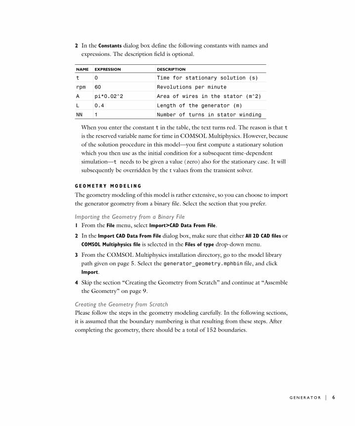
2 In the Constants dialog box define the following constants with names and expressions. The description field is optional.

When you enter the constant t in the table, the text turns red. The reason is that t is the reserved variable name for time in COMSOL Multiphysics. However, because of the solution procedure in this model—you first compute a stationary solution which you then use as the initial condition for a subsequent time-dependent simulation—t needs to be given a value (zero) also for the stationary case. It will subsequently be overridden by the t values from the transient solver.

G E O M E T R Y M O D E L I N G

The geometry modeling of this model is rather extensive, so you can choose to import the generator geometry from a binary file. Select the section that you prefer.

Importing the Geometry from a Binary File1 From the File menu, select Import>CAD Data From File.

2 In the Import CAD Data From File dialog box, make sure that either All 2D CAD files or COMSOL Multiphysics file is selected in the Files of type drop-down menu.

3 From the COMSOL Multiphysics installation directory, go to the model library path given on page 5. Select the generator_geometry.mphbin file, and click Import.

4 Skip the section “Creating the Geometry from Scratch” and continue at “Assemble the Geometry” on page 9.

Creating the Geometry from ScratchPlease follow the steps in the geometry modeling carefully. In the following sections, it is assumed that the boundary numbering is that resulting from these steps. After completing the geometry, there should be a total of 152 boundaries.

NAME EXPRESSION DESCRIPTION

t 0 Time for stationary solution (s)

rpm 60 Revolutions per minute

A pi*0.02^2 Area of wires in the stator (m^2)

L 0.4 Length of the generator (m)

NN 1 Number of turns in stator winding



1 Choose Draw>Specify Objects>Circle to create circles with the following properties:

2 Choose Draw>Specify Objects>Rectangle to create rectangles with the following properties:

3 Open the Create Composite Object dialog box from the Draw menu or click on the toolbar button with the same name.

4 In the dialog box clear the Keep interior boundaries check box.

5 Type C2+C1*(R1+R2+R3+R4) in the Set formula edit field.

6 Click OK.

7 Open the Create Composite Object dialog box again and select the Keep interior

boundaries check box.

8 Type C4+CO1-C3 in the Set formula edit field.

9 Click OK.

10 Create two new circles according to the table below.

11 Click the Zoom Extents button to get a better view of the geometry.

12 Select the circles C1 and C2.

13 Press Ctrl+C to copy the circles.

14 Press Ctrl+V to paste the circles. Make sure that the displacements are zero and click OK.

NAME RADIUS BASE X Y ROTATION ANGLE

C1 0.3 Center 0 0 22.5

C2 0.235 Center 0 0 0

C3 0.225 Center 0 0 0

C4 0.4 Center 0 0 0

NAME WIDTH HEIGHT BASE X Y ROTATION ANGLE

R1 0.1 1 Center 0 0 0

R2 0.1 1 Center 0 0 45

R3 0.1 1 Center 0 0 90

R4 0.1 1 Center 0 0 135


C1 0.015 Center 0.025 0.275 0

C2 0.015 Center -0.025 0.275 0



15 Go to Draw>Modify>Rotate and type 45 in the Rotation angle edit field before clicking OK.

16 Repeat the last two steps but with rotation angles 90, 135, 180, −45, −90, and −135.

17 Select all objects by pressing Ctrl+A, then click the Union toolbar button.

18 From the Draw menu open the Object Properties dialog box. Type Stator in the Label edit field to give the created object a more user-friendly name.

19 Click OK.

20 Create four circles with the following properties:

21 Create four rectangles with the following properties:

22 Open the Create Composite Object dialog box and clear the Keep interior boundaries check box.

23 Type C2+C1*(R1+R2+R3+R4) in the Set formula edit field.

24 Click OK.

25 Open the Create Composite Object dialog box again and select the Keep interior

boundaries check box.

26 Type CO1+C3+C4 in the Set formula edit field.

27 Click OK.

28 Open the Object Properties dialog box from the Draw menu, then type Rotor in the Label edit field.

29 Click OK.


C1 0.215 Center 0 0 0

C2 0.15 Center 0 0 22.5

C3 0.15 Center 0 0 22.5

C4 0.225 Center 0 0 0

NAME WIDTH HEIGHT BASE X Y ROTATION ANGLE

R1 0.1 1 Center 0 0 22.5

R2 0.1 1 Center 0 0 -22.5

R3 0.1 1 Center 0 0 67.5

R4 0.1 1 Center 0 0 -67.5



The geometry in the Drawing area should now look like that in Figure 5.

Assemble the Geometry1 Open the Create Pairs dialog box from the Draw menu.

2 Select both objects (Stator and Rotor), and click OK.

Figure 5: Generator geometry.

You have now created two separate geometry objects in an assembly. You have also created an identity pair connecting the physics in the rotor and the stator. Using an assembly allows you to apply all settings independently on these two objects. This is necessary to allow a sliding mesh at the interface between the stator and rotor because the solution variable becomes discontinuous across that interface.

P H Y S I C S S E T T I N G S

1 From the Options menu point to Integration Coupling Variables and click Subdomain

Variables.



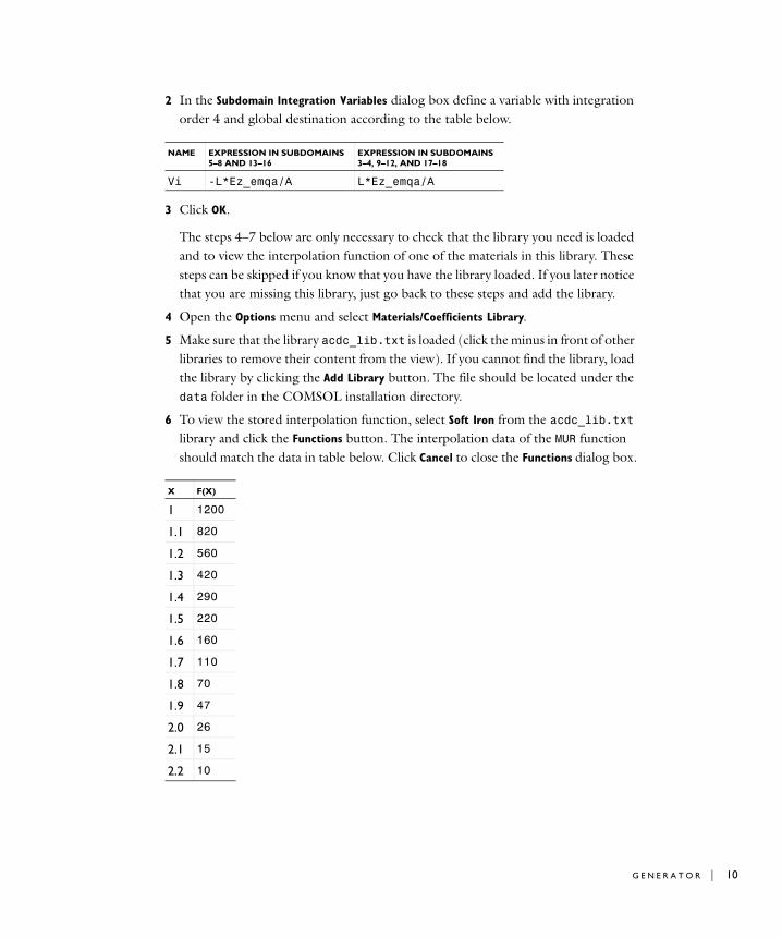
2 In the Subdomain Integration Variables dialog box define a variable with integration order 4 and global destination according to the table below.

3 Click OK.

The steps 4–7 below are only necessary to check that the library you need is loaded and to view the interpolation function of one of the materials in this library. These steps can be skipped if you know that you have the library loaded. If you later notice that you are missing this library, just go back to these steps and add the library.

4 Open the Options menu and select Materials/Coefficients Library.

5 Make sure that the library acdc_lib.txt is loaded (click the minus in front of other libraries to remove their content from the view). If you cannot find the library, load the library by clicking the Add Library button. The file should be located under the data folder in the COMSOL installation directory.

6 To view the stored interpolation function, select Soft Iron from the acdc_lib.txt library and click the Functions button. The interpolation data of the MUR function should match the data in table below. Click Cancel to close the Functions dialog box.

NAME EXPRESSION IN SUBDOMAINS 5–8 AND 13–16

EXPRESSION IN SUBDOMAINS 3–4, 9–12, AND 17–18

Vi -L*Ez_emqa/A L*Ez_emqa/A

X F(X)

1 1200

1.1 820

1.2 560

1.3 420

1.4 290

1.5 220

1.6 160

1.7 110

1.8 70

1.9 47

2.0 26

2.1 15

2.2 10



7 Click OK to close the Materials/Coefficients Library dialog box.

Subdomain Settings1 From the Multiphysics menu select Perpendicular Induction Currents (emqa) if it is not

already selected.

2 Choose Physics>Properties.

3 In the Properties dialog box choose Ideal from the Weak constraints list.

4 Click OK.

5 From the Physics menu open the Subdomain Settings, then select any entry in the Subdomain selection list.

6 Click the Load button to open the Materials/Coefficients Library dialog box.

7 In the dialog box select the Soft Iron material from the acdc_lib.txt library.

8 Click Apply. The material Soft Iron has now been added to the model. You see which materials you have added to the model under the Model item in the Materials tree view.

9 Repeat the last two steps for the materials Samarium Cobalt (Radial, inward) and Samarium Cobalt (Radial, outward). Before you close the dialog box, make sure that you see all three materials under Model in the Materials tree view.

10 Click Cancel to close the Materials/Coefficients Library dialog box.

11 Enter subdomain settings and select materials according to the table below. In order to use a remanent flux density, you need to click the option button for B = µ0µrH + Br first.

12 Click the Init tab, select all subdomains, and type sqrt(X^2+Y^2) in the Magnetic

potential, z component edit field.

13 Click OK.

14 From the Multiphysics menu select Moving mesh (ALE) (ale).

15 From the Physics menu open the Subdomain Settings.

2.3 7

2.4 6

SUBDOMAIN 20, 23, 24, 27 21, 22, 25, 26 2, 28 ALL OTHERS

Constitutive relation B = µ0µrH + Br B = µ0µrH + Br B = µ0µrH B = µ0µrH

Material Samarium Cobalt (Radial, inward)

Samarium Cobalt (Radial, outward)

Soft Iron

X F(X)



16 Select subdomains 19–28, then select the predefined group rotation_CCW from the Group list.

This group uses a prescribed displacement with expressions that define counter-clock-wise rotation around the origin. The default setting for all other subdomains is no displacement.

17 Click OK to close the dialog box.

Boundary ConditionsLeave the boundary settings at their defaults. The identity pair creates a coupling between the rotor and the stator in the ALE frame.

M E S H G E N E R A T I O N

1 Open the Free Mesh Parameters dialog box from the Mesh menu.

2 From the Predefined mesh sizes list select Finer.

3 Click the Custom mesh size option button and type 2 in the Resolution of narrow

regions edit field.

4 Click Remesh to generate the mesh.

5 Click OK to close the dialog box.

C O M P U T I N G T H E S O L U T I O N

Begin by computing the initial solution for the subsequent time-dependent simulation.

1 Open the Solver Parameters dialog box by clicking the corresponding button on the Main toolbar or from the Solve menu.

2 With the Auto select solver check box selected, select Static from the Analysis list.



3 Click OK.

4 Click the Solve button.

Next, simulate the generator with the rotor in motion. By default, the solution you just calculated will be used as the initial solution.

1 Open the Solver Parameters dialog box again and select Transient from the Analysis

list.

2 In the Times edit field type linspace(0,0.25,26), and in the Absolute tolerance edit field type Az 1e-3 lm1 5e3.

3 Click OK.

4 Click the Restart button.

PO S T P R O C E S S I N G A N D V I S U A L I Z A T I O N

1 From the Postprocessing menu open the Plot Parameters dialog box.

2 On the General page select the solution for time 0.2 s from the Solution at time list. Clear the Geometry edges check box.

3 On the Surface page select Magnetic flux density, norm from the Predefined quantities list or type normB_emqa in the Expression edit field.

4 On the Contour page type Az in the Expression edit field and type 15 in the Levels edit field. Click to select the Contour plot check box.



5 In the Contour color area select the Uniform color option button, and clear the Color

scale check box.

6 Click the Color button and select a black color. Click OK to close the Color dialog box.

7 On the Boundary page type 1 in the Expression edit field. Click to select the Boundary

plot check box.

8 In the Boundary color area select the Uniform color option button.

9 Click the Color button and select a black color. Click OK to close the Color dialog box.

10 Click OK to close the Plot Parameters dialog box.

To view the induced voltage as a function of time, proceed with the steps below.

1 From the Postprocessing menu, select Domain Plot Parameters.

2 On the Point page select an arbitrary point in the Point selection list, then type Vi*NN in the Expression edit field.

3 Click OK.

To create an animation of the rotating rotor, do the following steps.

1 Open the Plot Parameters dialog box.

2 Click the Animate tab and make sure that all time steps are selected.



3 Click the Start Animation button. When the movie has been generated, the COMSOL Movie Player opens it.


generator - Vaasan yliopistolipas.uwasa.fi/~mave/SAH104/generator.pdf · This is a true...

Documents

Transcript of generator - Vaasan yliopistolipas.uwasa.fi/~mave/SAH104/generator.pdf · This is a true...