Generating Dynamic Verification Tools for GeneralizedSymbolic Trajectory Evaluation (GSTE)

by

Kelvin Kwok Cheung Ng

B.A.Sc., University of British Columbia, 2001

A THESIS SUBMITTED IN PARTIAL FULFILLMENT OF

THE REQUIREMENTS FOR THE DEGREE OF

Master of Science

in

THE FACULTY OF GRADUATE STUDIES

(Department of Computer Science)

we accept this thesis as conformingto the required standard

The University of British ColumbiaAugust 2004

c© Kelvin Kwok Cheung Ng, 2004

Abstract

Formal and dynamic (simulation, emulation, etc.) verification techniques are both

needed to deal with the overall challenge of verification. Unfortunately, the same speci-

fication does not always work with both techniques. In particular, Generalized Symbolic

Trajectory Evaluation (GSTE) is a powerful formal verification technique developed by In-

tel and successfully used on next-generation microprocessor designs, but the specification

formalism for GSTE relies on “symbolic constants”, which intrinsically exploit the underly-

ing formal verification engine and cannot be reasonably handled via non-symbolic means.

In this thesis, I propose a modified version of GSTE specifications and present efficient,

automatic constructions to convert from the new simulation-friendly GSTE specifications

into conventional GSTE specifications (to access the formal verification tool flow) as well

as into monitor circuits suitable for conventional dynamic verification. I also investigate the

construction from the monitor circuits into testbench generator circuits. I implemented the

proposed constructions to demonstrate that my approach is practical and efficient.

ii

Contents

Abstract ii

Contents iii

List of Tables v

List of Figures vi

Acknowledgments vii

Dedication viii

1 Introduction 1

1.1 Motivation . . . . . . . . . . . . . . . . . . . . . . . . . . . . . . . . . . . 1

1.2 Research and Contributions . . . . . . . . . . . . . . . . . . . . . . . . . . 2

1.3 Thesis Outline . . . . . . . . . . . . . . . . . . . . . . . . . . . . . . . . . 3

2 Background 4

2.1 Generalized Symbolic Trajectory Evaluation (GSTE) . . . . . . . . . . . . 4

2.1.1 GSTE Assertion Graphs . . . . . . . . . . . . . . . . . . . . . . . 5

2.1.2 Symbolic Constants . . . . . . . . . . . . . . . . . . . . . . . . . 7

2.1.3 Retriggering and Knots . . . . . . . . . . . . . . . . . . . . . . . . 9

2.2 Dynamic Verification . . . . . . . . . . . . . . . . . . . . . . . . . . . . . 11

iii

2.2.1 Monitor Circuits . . . . . . . . . . . . . . . . . . . . . . . . . . . 12

2.2.2 Previous Work on Monitor Generation for GSTE . . . . . . . . . . 13

2.2.3 Testbench Generation . . . . . . . . . . . . . . . . . . . . . . . . . 14

3 Simulation-Friendly Assertion Graphs 15

4 Monitor Circuit Construction 20

4.1 Hardware Implementation . . . . . . . . . . . . . . . . . . . . . . . . . . 23

4.1.1 Vertices . . . . . . . . . . . . . . . . . . . . . . . . . . . . . . . . 24

4.1.2 Edges . . . . . . . . . . . . . . . . . . . . . . . . . . . . . . . . . 26

4.1.3 Instance Manager . . . . . . . . . . . . . . . . . . . . . . . . . . . 27

4.1.4 Monitor Output . . . . . . . . . . . . . . . . . . . . . . . . . . . . 30

4.2 Special Case: k = 1 . . . . . . . . . . . . . . . . . . . . . . . . . . . . . . 30

4.3 Bounding k . . . . . . . . . . . . . . . . . . . . . . . . . . . . . . . . . . 31

5 Experimental Results 32

5.1 Simulation Friendliness in Real Life . . . . . . . . . . . . . . . . . . . . . 33

5.2 Comparison with Previous Construction . . . . . . . . . . . . . . . . . . . 34

5.3 Effect of Changing the Parameter k . . . . . . . . . . . . . . . . . . . . . . 35

5.4 Real Industrial Example . . . . . . . . . . . . . . . . . . . . . . . . . . . 41

6 Testbench Generation 42

7 Conclusions and Future Work 46

Bibliography 48

iv

List of Tables

5.1 Results for Memory Example . . . . . . . . . . . . . . . . . . . . . . . . . 36

5.2 Results for FIFO Example . . . . . . . . . . . . . . . . . . . . . . . . . . 37

v

List of Figures

2.1 Generic Example Circuit . . . . . . . . . . . . . . . . . . . . . . . . . . . 5

2.2 Generic Example Assertion Graph . . . . . . . . . . . . . . . . . . . . . . 6

2.3 Simple Adder Assertion Graph (1+1=2) . . . . . . . . . . . . . . . . . . . 7

2.4 Simple Adder Assertion Graph (A+B=C) . . . . . . . . . . . . . . . . . . 8

2.5 Simple Adder Assertion Graph (A-B+B=A) . . . . . . . . . . . . . . . . . 9

2.6 Example Pipelined Assertion Graph . . . . . . . . . . . . . . . . . . . . . 10

3.1 Example of Simulation-Friendly Assertion Graph . . . . . . . . . . . . . . 17

3.2 Example of Traditional Assertion Graph . . . . . . . . . . . . . . . . . . . 17

4.1 An Algorithm for Finding Instance Edges in Assertion Graph G . . . . . . 24

5.1 Monitor Size vs. Previous Construction for FIFO Example . . . . . . . . . 38

5.2 Monitor Size vs. Previous Construction for Memory Example . . . . . . . 39

5.3 Monitor Scaling with k . . . . . . . . . . . . . . . . . . . . . . . . . . . . 40

vi

Acknowledgments

My thesis supervisor, Dr. Alan J. Hu, demonstrated in his thesis how to write acknowl-

edgments without mentioning and therefore excluding names of people who deserved his

thanks. While I intend to follow his great example, I would like to give my special thanks

to him, not only for coming up with such a brilliant idea, but more importantly for intro-

ducing me to the interesting world of hardware formal verification and providing me good

advice and tremendous support that are essential to my successful completion of the M.Sc.

program.

I consider myself fortunate to have been surrounded by great people for the past

few years. To all of you who have brought me so much joy, encouragement, and meaning,

thank you very much. While your names are not written down, the memories you gave me

will always remain in my heart.

KELVIN KWOK CHEUNG NG

The University of British Columbia

August 2004

vii

To my parents, for always loving me and supporting my decisions.

viii

Chapter 1

Introduction

1.1 Motivation

Formal verification and dynamic verification (i.e., simulation, emulation, etc.) are both

needed to deal with the overall challenge of verification. Formal techniques provide un-

paralleled coverage, whereas dynamic techniques have superior capacity, ramp-up more

quickly, and support more detailed modeling. Ideally, the same specification/testbench

would work with both formal and dynamic techniques, with the same semantics in both,

allowing a methodology that seamlessly chooses whatever technique is most appropriate

at any given point in the verification process. Unfortunately, this is typically not the case:

formal specifications often have a declarative aspect that can be difficult to convert to the

operational style needed for dynamic verification, and vice versa.

A particularly convenient bridge between formal and dynamic specifications is the

monitor circuit or assertion monitor. A monitor is simply a small circuit that watches,

without interfering, the system being verified and flags whether or not the system is obeying

a formal correctness property. Monitor circuits have the declarative style of typical formal

specifications, yet are operational and can be used with conventional scalar simulation.

Implementing the monitor as a circuit allows the same monitor to be used at all levels of the

design cycle and with both formal and informal verification tools.

1

Extensive research has demonstrated the value of monitor circuits as the cornerstone

of a practical verification methodology [1], as an enabler of hierarchical, compositional ver-

ification [8, 17, 7], and as a testbench generator for simulation [24]. Monitor circuits could

even be synthesized into an emulation system to aid error observability and debugging.

In my research, I focus on Generalized Symbolic Trajectory Evaluation

(GSTE) [20]1. GSTE was developed by Intel and is emerging as an important formal verifi-

cation technique that has been successful on leading-edge designs in industry, where users

reported superior efficiency and capacity (e.g., [2]), as well as having demonstrated effi-

ciency advantages in academic research [14].

GSTE uses a particular specification formalism, called an assertion graph, and the

efficiency of GSTE depends, in part, on the specifics of assertion graphs. Assertion graphs,

in turn, rely on a concept called “symbolic constants” (described in Chapter 2), which intrin-

sically exploit the underlying formal verification engine. Furthermore, when specifications

become retriggerable and multi-threaded, the semantics of symbolic constants become even

more complex. Previous work building monitor circuits for GSTE assertion graphs could

not handle symbolic constants, so the resulting monitor “circuit” needed a symbolic simu-

lator to have correct (i.e., agreeing with the formal verification) simulation semantics [5].

1.2 Research and Contributions

In this thesis, I address the problem of translating GSTE specifications into two dynamic

verification tools: monitor and testbench generator circuits. I first propose a modified ver-

sion of GSTE assertion graphs with clearer (but somewhat restricted) semantics for sym-

bolic constants. I then present efficient, automatic constructions to convert from the new

simulation-friendly GSTE specifications into traditional GSTE specifications, as well as

into monitor circuits completely suitable for conventional dynamic verification, without the

need for symbolic simulation. I demonstrate empirically that my simulation-friendly spec-

1GSTE is important in its own right, but I also hope that these ideas can prove helpful for otherspecification formalisms.

2

ification style is expressive enough for almost all real GSTE specifications, and that my

monitor construction is linear-size, imposing minimal overhead over the previously pub-

lished partially-symbolic monitor construction. I also investigate the problem of translating

GSTE specifications into testbench generator circuits.

1.3 Thesis Outline

This thesis is organized as follows. Chapter 2 introduces relevant background material and

prior work on the subject. Chapter 3 proposes a modified version of GSTE specifications,

named simulation-friendly assertion graphs and shows how to automatically translate from

this new specification style into the original GSTE one. Chapter 4 presents a construc-

tion of monitor circuits from simulation-friendly assertion graphs. The generated monitor

circuits are compatible with conventional dynamic verification, particularly scalar simula-

tion. Chapter 5 discusses experimental results related to the previous chapters. Chapter 6

describes an attempt to further extend the work into automatic construction of testbench

generator circuits. Chapter 7 consists of conclusions and future work.

3

Chapter 2

Background

As this thesis focuses on bridging the gap between formal verification (GSTE in particular)

and dynamic verification, I introduce in this chapter concepts and prior work related to my

thesis research. The first part of this chapter covers the basics of GSTE, a relatively new but

important formal verification method. The second part provides information on the other

world of verification – dynamic verification, as well as previous efforts to connect formal

and dynamic verification.

2.1 Generalized Symbolic Trajectory Evaluation (GSTE)

GSTE [20, 21, 19] is a recently developed model-checking [3, 13] method. It is an ex-

tension of Symbolic Trajectory Evaluation (STE) [15], which is efficient but has limited

expressiveness. One notable limitation is that STE cannot handle infinite time properties.

For example, STE cannot reason about a stall signal for stalling circuit operation, which

may be asserted for an indefinite length of time. An STE property consists of two parts,

an antecedent and a consequent, both describe relationship among system signals and may

contain finite-time temporal operators. The property holds when one of the following cases

happens: 1) both the antecedent and the consequent are true, or 2) the antecedent is false.

Intuitively, the property is like an if-then statement. If the conditions specified by the an-

4

nn n

stall

in0in1

out

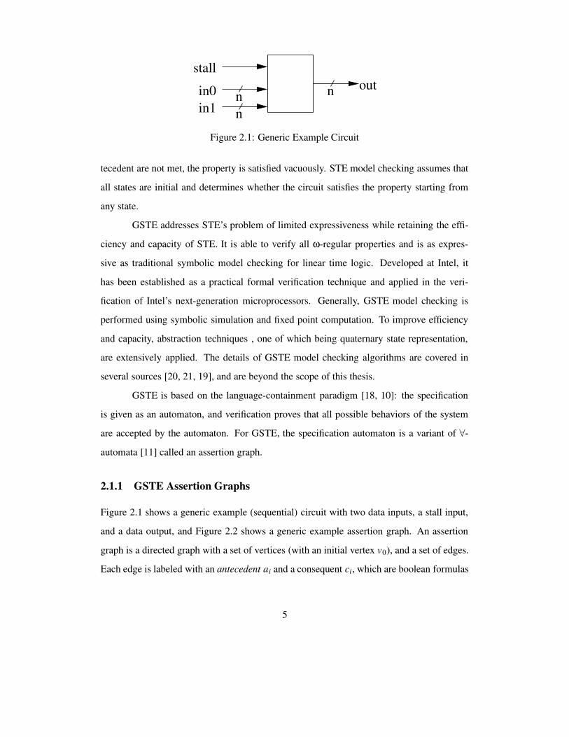
Figure 2.1: Generic Example Circuit

tecedent are not met, the property is satisfied vacuously. STE model checking assumes that

all states are initial and determines whether the circuit satisfies the property starting from

any state.

GSTE addresses STE’s problem of limited expressiveness while retaining the effi-

ciency and capacity of STE. It is able to verify all ω-regular properties and is as expres-

sive as traditional symbolic model checking for linear time logic. Developed at Intel, it

has been established as a practical formal verification technique and applied in the veri-

fication of Intel’s next-generation microprocessors. Generally, GSTE model checking is

performed using symbolic simulation and fixed point computation. To improve efficiency

and capacity, abstraction techniques , one of which being quaternary state representation,

are extensively applied. The details of GSTE model checking algorithms are covered in

several sources [20, 21, 19], and are beyond the scope of this thesis.

GSTE is based on the language-containment paradigm [18, 10]: the specification

is given as an automaton, and verification proves that all possible behaviors of the system

are accepted by the automaton. For GSTE, the specification automaton is a variant of ∀-

automata [11] called an assertion graph.

2.1.1 GSTE Assertion Graphs

Figure 2.1 shows a generic example (sequential) circuit with two data inputs, a stall input,

and a data output, and Figure 2.2 shows a generic example assertion graph. An assertion

graph is a directed graph with a set of vertices (with an initial vertex v0), and a set of edges.

Each edge is labeled with an antecedent ai and a consequent ci, which are boolean formulas

5

v2v0 v1a0 / c0

a1 / c1

a2 / c2

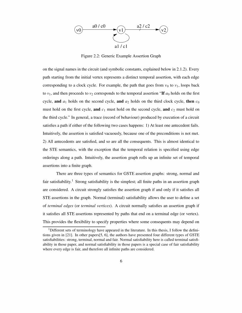
Figure 2.2: Generic Example Assertion Graph

on the signal names in the circuit (and symbolic constants, explained below in 2.1.2). Every

path starting from the initial vertex represents a distinct temporal assertion, with each edge

corresponding to a clock cycle. For example, the path that goes from v0 to v1, loops back

to v1, and then proceeds to v2 corresponds to the temporal assertion “If a0 holds on the first

cycle, and a1 holds on the second cycle, and a2 holds on the third clock cycle, then c0

must hold on the first cycle, and c1 must hold on the second cycle, and c2 must hold on

the third cycle.” In general, a trace (record of behaviour) produced by execution of a circuit

satisfies a path if either of the following two cases happens: 1) At least one antecedent fails.

Intuitively, the assertion is satisfied vacuously, because one of the preconditions is not met.

2) All antecedents are satisfied, and so are all the consequents. This is almost identical to

the STE semantics, with the exception that the temporal relation is specified using edge

orderings along a path. Intuitively, the assertion graph rolls up an infinite set of temporal

assertions into a finite graph.

There are three types of semantics for GSTE assertion graphs: strong, normal and

fair satisfiability.1 Strong satisfiability is the simplest; all finite paths in an assertion graph

are considered. A circuit strongly satisfies the assertion graph if and only if it satisfies all

STE assertions in the graph. Normal (terminal) satisfiability allows the user to define a set

of terminal edges (or terminal vertices). A circuit normally satisfies an assertion graph if

it satisfies all STE assertions represented by paths that end on a terminal edge (or vertex).

This provides the flexibility to specify properties where some consequents may depend on

1Different sets of terminology have appeared in the literature. In this thesis, I follow the defini-tions given in [21]. In other papers[5, 6], the authors have presented four different types of GSTEsatisfiabilities: strong, terminal, normal and fair. Normal satisfiability here is called terminal satisfi-ability in those paper, and normal satisfiability in those papers is a special case of fair satisfiabilitywhere every edge is fair, and therefore all infinite paths are considered.

6

v0 v1 v2

in0=1 & in1=1& !stall / true

stall / true

!stall / out=2

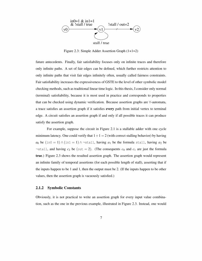
Figure 2.3: Simple Adder Assertion Graph (1+1=2)

future antecedents. Finally, fair satisfiability focuses only on infinite traces and therefore

only infinite paths. A set of fair edges can be defined, which further restricts attention to

only infinite paths that visit fair edges infinitely often, usually called fairness constraints.

Fair satisfiability increases the expressiveness of GSTE to the level of other symbolic model

checking methods, such as traditional linear time logic. In this thesis, I consider only normal

(terminal) satisfiability, because it is most used in practice and corresponds to properties

that can be checked using dynamic verification. Because assertion graphs are ∀-automata,

a trace satisfies an assertion graph if it satisfies every path from initial vertex to terminal

edge. A circuit satisfies an assertion graph if and only if all possible traces it can produce

satisfy the assertion graph.

For example, suppose the circuit in Figure 2.1 is a stallable adder with one cycle

minimum latency. One could verify that 1+1 = 2 (with correct stalling behavior) by having

a0 be (in0 = 1)∧ (in1 = 1)∧¬stall, having a1 be the formula stall, having a2 be

¬stall, and having c2 be (out = 2). (The consequents c0 and c1 are just the formula

true.) Figure 2.3 shows the resulted assertion graph. The assertion graph would represent

an infinite family of temporal assertions (for each possible length of stall), asserting that if

the inputs happen to be 1 and 1, then the output must be 2. (If the inputs happen to be other

values, then the assertion graph is vacuously satisfied.)

2.1.2 Symbolic Constants

Obviously, it is not practical to write an assertion graph for every input value combina-

tion, such as the one in the previous example, illustrated in Figure 2.3. Instead, one would

7

v0 v1 v2& !stall / true

stall / true

in0=A & in1=B !stall / out=B

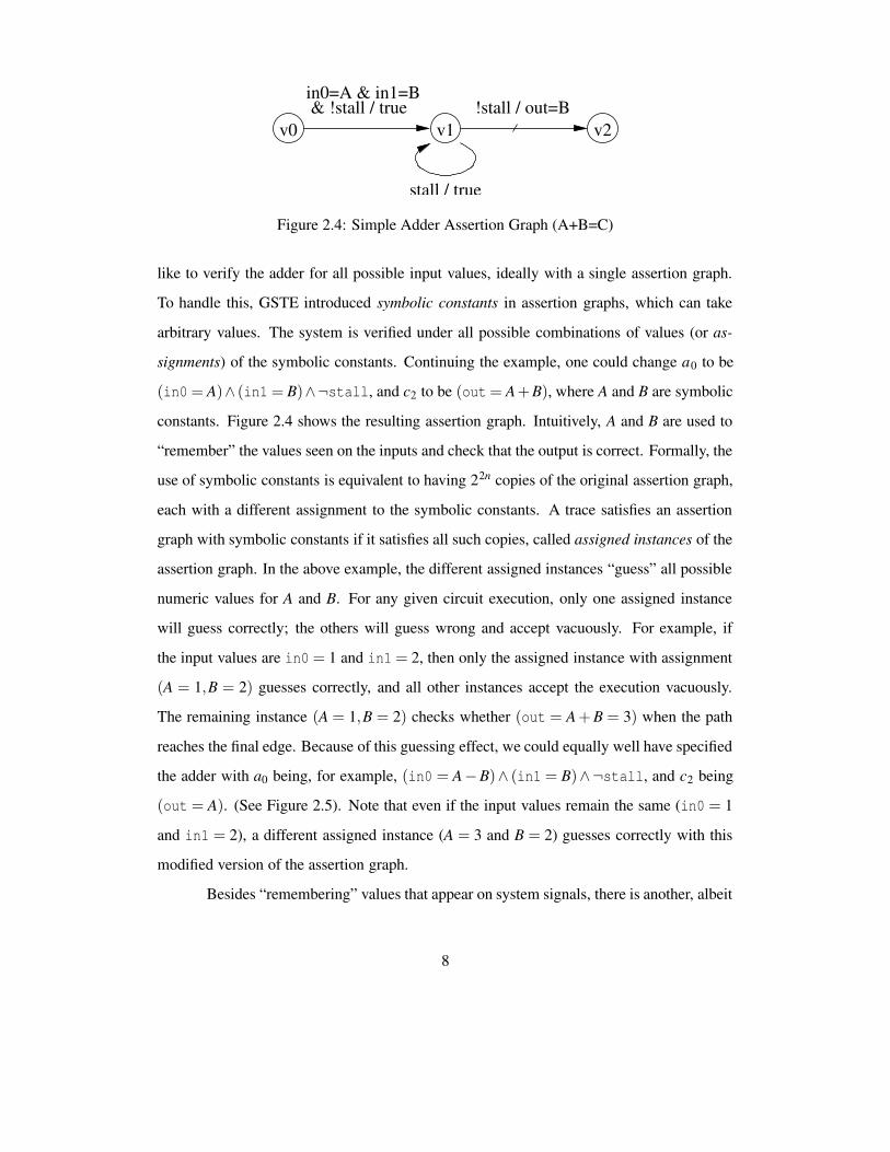
Figure 2.4: Simple Adder Assertion Graph (A+B=C)

like to verify the adder for all possible input values, ideally with a single assertion graph.

To handle this, GSTE introduced symbolic constants in assertion graphs, which can take

arbitrary values. The system is verified under all possible combinations of values (or as-

signments) of the symbolic constants. Continuing the example, one could change a0 to be

(in0 = A)∧ (in1 = B)∧¬stall, and c2 to be (out = A+B), where A and B are symbolic

constants. Figure 2.4 shows the resulting assertion graph. Intuitively, A and B are used to

“remember” the values seen on the inputs and check that the output is correct. Formally, the

use of symbolic constants is equivalent to having 22n copies of the original assertion graph,

each with a different assignment to the symbolic constants. A trace satisfies an assertion

graph with symbolic constants if it satisfies all such copies, called assigned instances of the

assertion graph. In the above example, the different assigned instances “guess” all possible

numeric values for A and B. For any given circuit execution, only one assigned instance

will guess correctly; the others will guess wrong and accept vacuously. For example, if

the input values are in0 = 1 and in1 = 2, then only the assigned instance with assignment

(A = 1,B = 2) guesses correctly, and all other instances accept the execution vacuously.

The remaining instance (A = 1,B = 2) checks whether (out = A + B = 3) when the path

reaches the final edge. Because of this guessing effect, we could equally well have specified

the adder with a0 being, for example, (in0 = A−B)∧ (in1 = B)∧¬stall, and c2 being

(out = A). (See Figure 2.5). Note that even if the input values remain the same (in0 = 1

and in1 = 2), a different assigned instance (A = 3 and B = 2) guesses correctly with this

modified version of the assertion graph.

Besides “remembering” values that appear on system signals, there is another, albeit

8

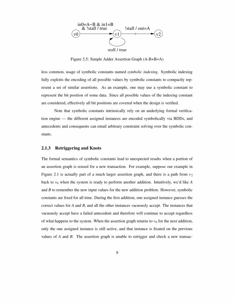
v0 v1 v2& !stall / true

stall / true

in0=A−B & in1=B !stall / out=A

Figure 2.5: Simple Adder Assertion Graph (A-B+B=A)

less common, usage of symbolic constants named symbolic indexing. Symbolic indexing

fully exploits the encoding of all possible values by symbolic constants to compactly rep-

resent a set of similar assertions. As an example, one may use a symbolic constant to

represent the bit position of some data. Since all possible values of the indexing constant

are considered, effectively all bit positions are covered when the design is verified.

Note that symbolic constants intrinsically rely on an underlying formal verifica-

tion engine — the different assigned instances are encoded symbolically via BDDs, and

antecedents and consequents can entail arbitrary constraint solving over the symbolic con-

stants.

2.1.3 Retriggering and Knots

The formal semantics of symbolic constants lead to unexpected results when a portion of

an assertion graph is reused for a new transaction. For example, suppose our example in

Figure 2.1 is actually part of a much larger assertion graph, and there is a path from v2

back to v0 when the system is ready to perform another addition. Intuitively, we’d like A

and B to remember the new input values for the new addition problem. However, symbolic

constants are fixed for all time. During the first addition, one assigned instance guesses the

correct values for A and B, and all the other instances vacuously accept. The instances that

vacuously accept have a failed antecedent and therefore will continue to accept regardless

of what happens to the system. When the assertion graph returns to v0 for the next addition,

only the one assigned instance is still active, and that instance is fixated on the previous

values of A and B. The assertion graph is unable to retrigger and check a new transac-

9

v1

stall / true

v2

stall / true

v3v0

true / true

a0 / true !stall / true !stall / c2

Figure 2.6: Example Pipelined Assertion Graph

tion. This is because the assigned instances are independent, and therefore a valid path on

the assertion graph cannot contain more than one assignment to the symbolic constants.

Retriggering requires the flexibility to change values for every new transaction.

To address this problem, GSTE enhancements introduced the concept of knots to

assertion graphs. Intuitively, a knot is a point in the assertion graph where the value of a

symbolic constant is forgotten. The name knot arises because conceptually, the knot is a

point where the different assigned instances are “tied together”, allowing a path to move

from one assigned instance to another, with different values for symbolic constants. If we

introduce a knot at v0, the assertion graph becomes retriggerable. Formally, the values

of symbolic constants are existentially quantified when a path reaches a knot, effectively

making the path active in all assigned instances. The intended usage expects a knot to be

followed immediately by a special kind of antecedent, which reduces the number of active

assigned instances back to a small number, usually one. (in0 = A)∧ (in1 = B)∧¬stall

is an example of such antecedent. A knot can be made specific to a particular symbolic

constant or a subset of symbolic constants. This provides extra flexibility to reset only the

desired symbolic constant(s) at any point on the assertion graph.

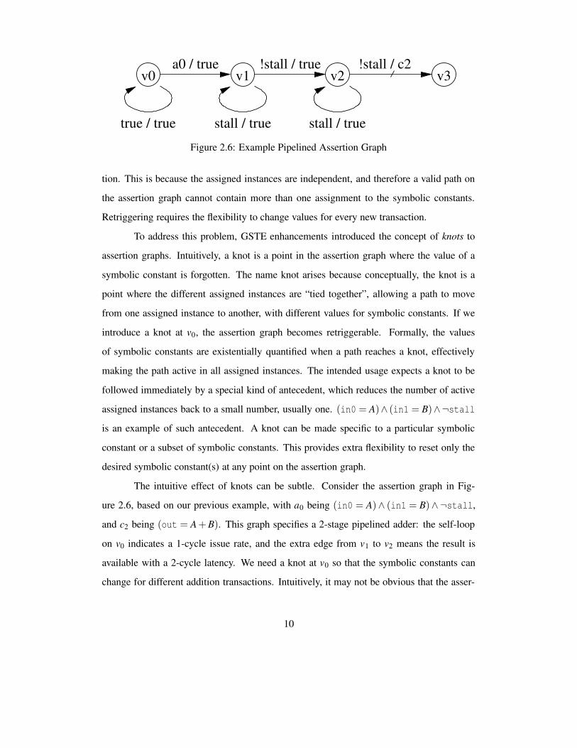
The intuitive effect of knots can be subtle. Consider the assertion graph in Fig-

ure 2.6, based on our previous example, with a0 being (in0 = A)∧ (in1 = B)∧¬stall,

and c2 being (out = A + B). This graph specifies a 2-stage pipelined adder: the self-loop

on v0 indicates a 1-cycle issue rate, and the extra edge from v1 to v2 means the result is

available with a 2-cycle latency. We need a knot at v0 so that the symbolic constants can

change for different addition transactions. Intuitively, it may not be obvious that the asser-

10

tion graph can keep the different copies of the symbolic constants distinct, but recall that

each assigned instance is effectively a separate copy of the assertion graph, so they do not

interfere. Furthermore, it may appear that we could make infinite-state assertion graphs by,

for example, changing a0 to be (in0= A)∧(in1= B), so that we can load new values every

clock cycle, while delaying the output of results by asserting stall. However, the resulting

assertion graph is actually finite-state, because the different instances will all get stuck on

the stall self-loops, where the temporal ordering of the different symbolic constant values

will be lost. The graph will record only the set of symbolic constant values that are possible

on each edge, which is extremely large, but still finite-state, rather than the sequence of

values, which is infinite-state.

2.2 Dynamic Verification

Dynamic verification (or validation) refers to verification by simulation or emulation of

hardware designs. Typically, engineers define a set of input stimuli, also called a testbench,

apply it to the design under verification by simulation or emulation, observe system re-

sponses, and then determine whether the displayed behaviours are expected and correct.

Dynamic verification is the standard practice for digital design verification and has been

widely accepted for generations of hardware engineers. It is well-understand, easy-to-use,

and scalable to handle large industrial designs. However, with increased design complex-

ity, dynamic verification covers too small a portion of the input space to provide enough

confidence within resource constraints. Even after engineers have carefully selected in-

put sequences in their testbench, many bugs remain uncovered. Formal verification, on

the other hand, provides unparalleled coverage but requires significant human effort before

producing useful results and is limited in the size and the complexity of designs it can han-

dle. Both formal and dynamic verification techniques are needed to meet the challenge of

verifying today’s complex designs.

While simulation and emulation are automatic with the help of software simulators

or hardware emulators, manual effort is still required to create a testbench and to examine

11

the results or define expected results. As designs grow in size and complexity, dynamic

verification becomes increasingly difficult and time-consuming, especially when human

productivity scales much more slowly than computing resources. It is desirable and even

necessary to automate dynamic verification as much as possible. This section introduces

tools to automate dynamic verification and describes previous effort to connect formal and

dynamic verification.

2.2.1 Monitor Circuits

A particularly useful tool for dynamic verification is a correctness checker. If implemented

in hardware, it is also called a monitor circuit. When connected to the system being verified,

a monitor circuit observes values at relevant system signals and determines whether a prop-

erty is satisfied in the current execution. A monitor can be used to define a desired property

of the system under verification, and it automatically decides whether the observed execu-

tion violates the property. It is declarative and independent of system implementation, yet

operational for conventional scalar simulation and can even be synthesized into an emula-

tion system to aid error observation and debugging. As a circuit, it can be used at all stages

of the design cycle and easily reused for different designs. Monitors have been proven to

be the cornerstone of a practical verification methodology [1]. They can also be combined

to enable hierarchical, compositional verification [8, 17, 7]. An important example of mon-

itor application is interface protocol verification, where the communication between two

hardware components is checked against a predefined protocol. A monitor circuit can be

connected to signals at the interface and used to determine whether the protocol is followed

during dynamic verification.

Monitors eliminate the need for designers to manually examine the simulation out-

put or manually define the expected outputs given the input sequence. The value of mon-

itors, however, would be significantly reduced if substantial amount of effort is required

to create practical monitor circuits. Fortunately, research has demonstrated that it is often

possible to automatically generate monitor circuits from formal specifications [8, 17, 7].

12

However, for more general formal specifications, GSTE in particular, previous work [5]

does not satisfactorily handle a large class of properties, namely those with symbolic con-

stants. A major part of my research is to build upon this piece of previous work, which

is explained below in Section 2.2.2, to generate useful monitor circuits for most assertion

graphs used in real life.

2.2.2 Previous Work on Monitor Generation for GSTE

This section describes a piece of previous work on generating monitor circuits for GSTE

assertion graphs [5]. Given the difficulties of handling symbolic constants without a formal

verification engine, the previous work does not adequately handle symbolic constants in

assertion graphs, requiring a symbolic simulator in those cases. On the other hand, it is

efficient for assertion graphs without symbolic constants and forms the basis of my new

monitor construction. Hence, I review the construction here.

Conceptually, the monitor circuit tracks all paths in the assertion graph and checks

each path cycle-by-cycle against the execution trace being monitored. To do so, the monitor

circuit structure is essentially a copy of the assertion graph, and the monitor circuit tracks

paths by moving tokens around the assertion graphs, where a token on an edge indicates

that there is a path that ends on that edge on that clock cycle. At each clock cycle, the

antecedent and consequent are evaluated for the current state in the execution trace, the

tokens are updated to record antecedent or consequent failures, and the tokens propagate to

the next possible edges. The key insight is that tokens can actually be almost memoryless.

The only history necessary is to distinguish between three different kinds of pasts: (1) if an

antecedent has failed already, this path and its continuations will always accept, so they need

not be tracked any further, (2) if all antecedents and all consequents so far have succeeded,

then this path currently accepts, but its continuations might not, and (3) if all antecedents

have succeeded, but at least one consequent has failed, then this path currently rejects, but

its continuations might eventually accept if an antecedent fails in the future. Paths of type

(1) are called “blessed”; type (2), “happy”; and type (3), “condemned” [5]. Moreover,

13

tokens of the same type that arrive at the same edge at the same time share the same future,

so they can be merged. Accordingly, the monitor circuit simply has two latches for each

edge of the assertion graph: one to track happy paths, and one to track condemned paths.

Simple combinational logic updates the tokens and propagates them. The monitor flags an

error if there is a condemned token on any terminal edge.

The hardware implementation follows closely the above intuition. Each vertex and

each edge has its own hardware module, connected as in the assertion graph. Edges and

vertices are connected by two signals, happy and condemned, to achieve the passing of

tokens and the recording of their history. Vertex modules are combinational, they only

merge tokens of the same type and forward outgoing token(s) by asserting the respective

signal(s). Edge modules contain latches so that results of antecedent/consequent evaluation

in the current cycle are reflected in the next cycle. The output logic is connected to all

terminal edges and indicates error whenever a condemned token arrives on any terminal

edge.

2.2.3 Testbench Generation

While a monitor observes the system being verified and decides whether the execution sat-

isfies some properly, it does not provide any input stimulus to drive simulation. Often,

a hardware unit is designed with assumptions on the input values and may not function

properly if the assumptions are violated. These assumptions are called input constraints.

Another very useful dynamic verification tool is an input generator, also called testbench

generator. A testbench generator automatically generates input sequence that satisfies a set

of input constraints. In addition, it may allow biasing of generated input values achieve

coverage goals set by its user. Extensive research has been performed on testbench genera-

tors for different styles of specifications [16, 24, 4, 22, 23], but no prior work has been done

for GSTE. In my research, I investigate the possibility to construct a testbench generator for

GSTE, and preferably from a monitor circuit.

14

Chapter 3

Simulation-Friendly Assertion

Graphs

Three main difficulties appear to prevent translating assertion graphs into monitor circuits

that require no symbolic simulation. First, symbolic constants initially take on all possible

values, and then the set of possible values is pruned essentially by constraint solving. The

antecedents act as the constraints to prune values, because typically antecedents that use

the symbolic constants are satisfied only with a small number of symbolic constant assign-

ments, and paths (and assigned instances) with failed antecedents need not be tracked. Sec-

ond, the semantics of knots are defined specifically according to the formal model — how

the exponential number of assigned instances interact. Knots enable retriggerable asser-

tions, but they increase complexity because assigned instances are no longer independent

of each other. Third, as we saw in Figure 2.6, assertion graphs can record an intractable

amount of history, such as the exact set of data values that have been seen, the worst case

size of which is exponential in the number of total symbolic constant values. These diffi-

culties mean that a fully general monitor construction for assertion graphs would need to

generate circuits that perform constraint solving and are exponential in the number of bits

of symbolic constants. Clearly, such a monitor circuit would not be practical. An additional

drawback of fully general assertion graphs is that the semantics can be unintuitive, requir-

15

ing a good understanding of the underlying formal model. A unified specification style for

formal and dynamic verification should be simpler to understand.

Fortunately, the assertion graphs I have observed in practice are not fully general. In

particular, in their typical usage, symbolic constants are used to record some information,

followed by subsequent use of the information. One may think of the symbolic constants

first being “assigned” to record some information, usually the values of some signals at

a particular time, and that information is used subsequently to define the GSTE property.

This intuitive usage is not only easy to understand; it also enables the possibility of creating

practical monitor circuits (explained in Chapter 4). To capture this concept, I define a new,

simulation-friendly style of GSTE assertion graphs.

A simulation-friendly assertion graph is a modified version of a traditional GSTE

assertion graph. It is exactly the same as a traditional assertion graph if symbolic constants

are not present. For simulation-friendly assertion graphs with symbolic constants, I intro-

duce explicit assignment statements, eliminate the knot construct, and impose a restriction.

Assignment statements can be placed on edges, and they assign to a symbolic constant some

value computed as an arithmetic/logical expression over the signal names in the circuit. The

assignment takes effect before the antecedent and consequent on that edge are evaluated.

Knots are not allowed in simulation-friendly assertion graphs, and assignment statements

provide a means to erase or reset values of symbolic constants, which is the intended usage

of knots. Technically, an antecedent following a knot can be fully general, and therefore re-

placing knots with assignments makes simulation-friendly assertion graphs less expressive

than traditional ones. However, the use of assignments corresponds nicely to the intended

and common usage of knots. I impose the additional restriction that on every path from the

initial vertex, each symbolic constant must be assigned before it is used. In other words,

when a path reaches an edge with a symbolic constant on its label, there is always a sin-

gle value for the symbolic constant, which is the latest assigned value. That value should

be used to evaluate the antecedent/consequent. Despite sacrificing the ability of symbolic

constants to represent all possible values in parallel, simulation-friendly assertion graphs

16

v0

true / true

v1

stall / true

v2

stall / true

v3!stall / true

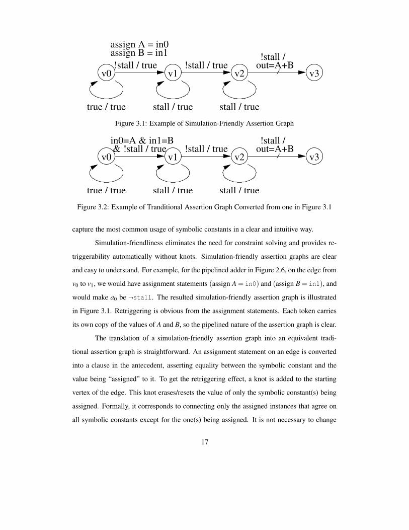
assign A = in0assign B = in1!stall / true out=A+B

!stall /

Figure 3.1: Example of Simulation-Friendly Assertion Graph

v0

true / true

!stall / truev1

stall / true

v2

stall / true

v3& !stall / truein0=A & in1=B

out=A+B!stall /

Figure 3.2: Example of Tranditional Assertion Graph Converted from one in Figure 3.1

capture the most common usage of symbolic constants in a clear and intuitive way.

Simulation-friendliness eliminates the need for constraint solving and provides re-

triggerability automatically without knots. Simulation-friendly assertion graphs are clear

and easy to understand. For example, for the pipelined adder in Figure 2.6, on the edge from

v0 to v1, we would have assignment statements (assign A = in0) and (assign B = in1), and

would make a0 be ¬stall. The resulted simulation-friendly assertion graph is illustrated

in Figure 3.1. Retriggering is obvious from the assignment statements. Each token carries

its own copy of the values of A and B, so the pipelined nature of the assertion graph is clear.

The translation of a simulation-friendly assertion graph into an equivalent tradi-

tional assertion graph is straightforward. An assignment statement on an edge is converted

into a clause in the antecedent, asserting equality between the symbolic constant and the

value being “assigned” to it. To get the retriggering effect, a knot is added to the starting

vertex of the edge. This knot erases/resets the value of only the symbolic constant(s) being

assigned. Formally, it corresponds to connecting only the assigned instances that agree on

all symbolic constants except for the one(s) being assigned. It is not necessary to change

17

the remaining parts of the assertion graph. The equivalent traditional assertion graph of the

previous example (Figure 3.1) is shown in Figure 3.2. With the easy translation, a user can

write assertion graphs in simulation-friendly style and access the GSTE formal verification

engine through the equivalent traditional assertion graphs.

While I claim that simulation-friendly assertion graphs are expressive enough for

practical use, a good way to test this claim is to see how many GSTE properties in real

life can be written in the simulation-friendly style. Unlike its counterpart in the opposite

direction, the translation from a traditional GSTE assertion graph into a simulation-friendly

one is not always straightforward. For assertion graphs that use symbolic constants in

the same manner that simulation-friendly assertion graphs do, the translation is simply a

replacement of knots and relevant antecedents with assignment statements. Unfortunately,

there are cases where translation is not as easy. For example, the use of symbolic constants

for symbolic indexing is not permitted in simulation-friendly assertion graphs. Once a

symbolic constant has been assigned, it loses the power to represent all possible values,

on which symbolic indexing depends. However, in general, if the number of indexing

constant bits is small, it is possible to convert the assertion graph into simulation-friendly

format by expanding the graph to eliminate the indexing constants. Section 5.1 discusses

the techniques involved. Also, an assignment statement allows a single assigned value to a

symbolic constant. If multiple assigned values are needed on the same edge, the edge have

to be duplicated the same number of times, each with a different assignment statement.

For example, if the antecedent on an edge following a knot is (A = 2)∨ (A = 3), where

A is a symbolic constant, the equivalent simulation-friendly assertion graph will have two

edges with identical source and destination vertices. The only difference is the assignment

statement, where one has (assign A = 2), the other has (assign A = 3).

The remaining questions include: (1) Are simulation-friendly assertion graphs gen-

eral enough to handle practical industrial usage? (2) Can we efficiently build monitor cir-

cuits for them that are compatible with conventional dynamic verification (no symbolic

simulation required)? And (3) how can we limit the size of the monitor circuit to avoid

18

recording intractable amounts of history information? I address the first question empiri-

cally in Chapter 5. That chapter also contains other experimental results on my proposed

monitor circuit construction. The next chapter addresses the other two questions by present-

ing a solution — a method to construct monitor circuits for simulation-friendly assertion

graphs.

19

Chapter 4

Monitor Circuit Construction

Simulation-friendly assertion graphs, introduced in Chapter 3, promise to enable construc-

tion of practical monitor circuits that do not require symbolic simulation. The central idea to

simulation-friendly assertion graphs is to replace knots with assignment statements. Com-

bined with the requirement that symbolic constants are assigned before use, it eliminates

the need to record an intractable amount of information. In the case of traditional assertion

graphs, any path in the beginning is active in all assigned instances, and the number of as-

signed instances with an active copy of a path can remain large (exponential in the number

of symbolic constant bits in the worst case) for a long time. In contrast, for simulation-

friendly assertion graphs, assignment statements enforce a single active value for any sym-

bolic constant on a path. To be precise, a new value is required when a path (or a branch

of a path) visits an assignment statement. Moreover, an old value can be cleared as soon

as it is not needed. In theory, the number of active symbolic constants could still approach

the same worst case, but in practice, it is still a lot more manageable than tracking paths

in all assigned instances initially. This chapter presents an efficient construction of moni-

tor circuits for simulation-friendly assertion graphs. The generated monitor circuits work

with conventional (non-symbolic) simulation and emulation. Overall, the construction for

simulation-friendly assertion graphs is based on the one proposed in [5] (also explained

briefly in Section 2.2.2), with added complexity to properly handle symbolic constants.

20

The monitor circuit observes the system under verification and determines whether

the execution trace is legal according to its associated simulation-friendly assertion graph.

A trace is legal when it satisfies the property described by the assertion graph. The input

signal reset, initializes the monitor for a new trace when asserted. A new trace starts when

the reset signal falls from high to low. The monitor inputs also include system signals

that appear on antecedents and consequents. The monitor circuit has two output signals,

accept and overflow. The accept signal is asserted when the monitor accepts the trace

for satisfying the assertion graph, and deasserted when the trace violates the property. The

overflow signal is asserted only when the monitor determines it has run out of storage

space to monitor system execution, rendering the accept output value incorrect. During

monitor construction, the user provides a constant k, the maximum number of assigned in-

stances that the monitor can handle at a time. This limits the amount of history information

the monitor needs to store, which directly affects its size. Section 4.3 contains a discussion

on determining the value of k. The overflow signal indicates whether the current trace

requires more than k simultaneously active assigned instances.

Intuitively, the monitor circuit has an internal copy of the assertion graph and uses

tokens to track relevant paths. It starts by placing a token on every outgoing edge of the

initial vertex (and clearing tokens on the rest). A token arriving on an edge means that at

least one path ends on that edge, on that cycle. Tokens also carry history information about

their represented paths. An edge receiving a token checks its antecedent/consequent and

forwards a token to its outgoing edge(s) on the next cycle if necessary. Multiple tokens

arriving on the same edge at the same time are merged into a single token if those paths

share the same future. To determine trace acceptance, the monitor checks the terminal

edges for any token that suggests violation of the assertion.

Following the terminology in [5], there are three types of paths: blessed, happy

and condemned. A blessed path has at least one failed antecedent and therefore accepts

the trace vacuously. Furthermore, any extension of a blessed path is also blessed. Hence,

once a path is blessed, it needs not be recorded further. A happy path has all its antecedents

21

and consequents satisfied and therefore accepts the current trace. However, the future is

unknown. Extensions of a happy path may accept or reject the continued trace and can be

of any type. A condemned path has all its antecedents satisfied but at least one consequent

failed. A condemned path rejects the current trace, but its extensions may be blessed (but

not happy). When any token arrives on an edge and the antecedent fails, the represented

path(s) and all its(their) extensions are blessed. The token disappears on the next cycle.

When a happy token arrives, an edge forwards a happy token to its outgoing edges only if

both the antecedent and the consequent hold. If the consequent fails, the edge forwards a

condemned token. An edge receiving a condemned token forwards a condemned token if

its antecedent holds. The monitor asserts its accept signal if and only if no condemned

token is generated on any terminal edge.

The paragraphs above describe the fundamental idea behind monitor circuits for

GSTE in general. It works well with assertion graphs with no symbolic constants, and

my proposed construction also follows this same idea to track paths in the assertion graph.

However, if one were to directly apply this idea to assertion graphs with symbolic constants,

the monitor circuits would have to contain not one but 2n copies of the assertion graph (n is

the total number of symbolic constant bits), one for each assigned instance. The resulting

monitor circuits would certainly be too big for most cases in practice. Fortunately, it is

possible to translate simulation-friendly assertion graphs into practical monitor circuits.

Because symbolic constants are assigned before use, a path does not have multiple copies

of itself with different symbolic constant values. Instead, a path only exists virtually in a

single assigned instance. To be exact, a path may exist in multiple assigned instances, but

only because of the unassigned symbolic constants. When the value of a symbolic constant

is needed to evaluate the antecedent/consequent on a path, only a single value needs to be

considered. This makes it possible to carry an assigned value of symbolic constants with

a token. Without the restriction required by simulation-friendliness, the monitor circuit

either needs multiple copies of the assertion graph or multiple values of symbolic constants

stored in the tokens. Both would make the size of monitor intractable, not to mention the

22

complexity of hardware to handle them.

In my proposed construction, there is only a single copy of the assertion graph in

the monitor circuit, and tokens are handled the same way as described before. The major

difference is that tokens also store assigned values, updated when tokens visit edges with

an assignment statement, or assigning edges. When evaluating the antecedent/consequent

on an edge, if a symbolic constant is mentioned, it must have been assigned and therefore

have its value stored in the token. The stored values are used for evaluation of the an-

tecedent/consequent (if necessary). This also means that tokens with different assigned val-

ues cannot be merged, even when they are of the same type (happy or blessed). A monitor

can support at most k different assigned values on all tokens at one time. A key optimiza-

tion, then, is to clear the assigned value on a token as soon as possible, i.e., when all future

edges the token may visit do not have symbolic constants on their antecedents/consequents.

It is straightforward to decide which edges should receive tokens with assigned values. We

will refer to them as instance edges, as opposed to simple edges, which do not need as-

signed values on tokens. Instance vertices are starting vertices of instance edges; simple

vertices are not. Figure 4.1 presents an algorithm for finding instance edges. In short, the

algorithm marks all edges that directly uses a symbolic constant and performs a background

traversal toward an assigning edge for the same constant, marking all edges along the way

except the assigning edges. It repeats this process for all symbolic constants, and all edges

marked at any time are instance edges. By releasing the storage for assigned values as soon

as possible, the monitor is able to use the same resources for other transactions.

4.1 Hardware Implementation

The hardware implementation closely follows the above intuition. The monitor circuit re-

sembles the assertion graph: there are modules for vertices and edges, connected in the

same way as in the assertion graph for passing tokens. The tokens are implemented as sig-

nals connecting edges and vertices. As there are two types of tokens to be passed around,

all edges and vertices are connected by at least two signals: happy and condemned. These

23

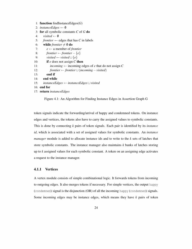
1: function findInstanceEdges(G)2: instanceEdges← /03: for all symbolic constants C of G do4: visited← /05: frontier ← edges that has C in labels6: while frontier 6= /0 do7: e← a member of frontier8: frontier← frontier−{e}9: visited← visited∪{e}

10: if e does not assign C then11: incoming← incoming edges of e that do not assign C12: frontier← frontier∪ (incoming− visited)13: end if14: end while15: instanceEdges← instanceEdges∪ visited16: end for17: return instanceEdges

Figure 4.1: An Algorithm for Finding Instance Edges in Assertion Graph G

token signals indicate the forwarding/arrival of happy and condemned tokens. On instance

edges and vertices, the tokens also have to carry the assigned values to symbolic constants.

This is done by connecting k pairs of token signals. Each pair is identified by its instance

id, which is associated with a set of assigned values for symbolic constants. An instance

manager module is added to allocate instance ids and to write to the k sets of latches that

store symbolic constants. The instance manager also maintains k banks of latches storing

up to k assigned values for each symbolic constant. A token on an assigning edge activates

a request to the instance manager.

4.1.1 Vertices

A vertex module consists of simple combinational logic. It forwards tokens from incoming

to outgoing edges. It also merges tokens if necessary. For simple vertices, the output happy

(condemned) signal is the disjunction (OR) of all the incoming happy (condemned) signals.

Some incoming edges may be instance edges, which means they have k pairs of token

24

signals. Those k pairs of token signals can be merged (by disjunction) because the assigned

values become irrelevant beyond this point in the assertion graph. After merging, they

are treated the same way as the other incoming signals (from simple edges). For instance

vertices, which outputs k pairs of token signals, there are always k pairs of input signals

from each incoming edge. (Otherwise, the assertion graph is not simulation-friendly.) Each

output signal is then the disjunction of the corresponding input signals of the same instance

id from different edges.

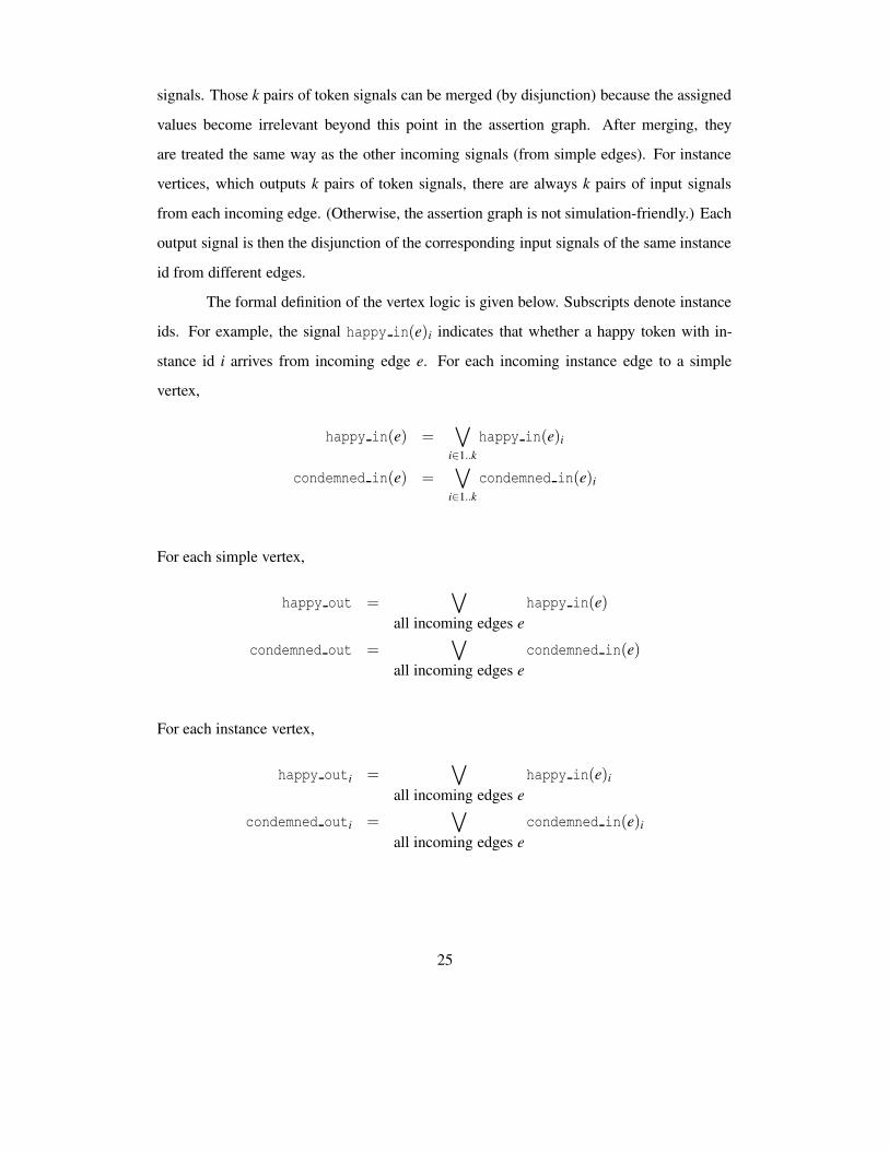
The formal definition of the vertex logic is given below. Subscripts denote instance

ids. For example, the signal happy in(e)i indicates that whether a happy token with in-

stance id i arrives from incoming edge e. For each incoming instance edge to a simple

vertex,

happy in(e) =_

i∈1..k

happy in(e)i

condemned in(e) =_

i∈1..k

condemned in(e)i

For each simple vertex,

happy out =_

all incoming edges ehappy in(e)

condemned out =_

all incoming edges econdemned in(e)

For each instance vertex,

happy outi =_

all incoming edges ehappy in(e)i

condemned outi =_

all incoming edges econdemned in(e)i

25

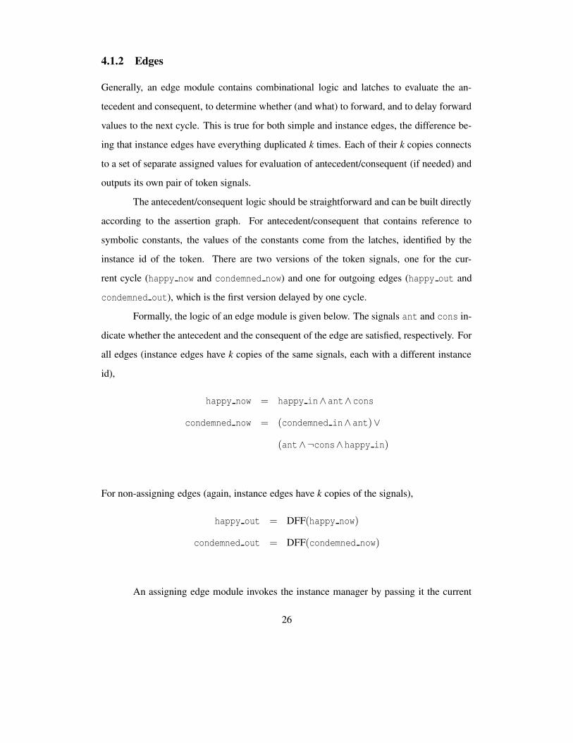
4.1.2 Edges

Generally, an edge module contains combinational logic and latches to evaluate the an-

tecedent and consequent, to determine whether (and what) to forward, and to delay forward

values to the next cycle. This is true for both simple and instance edges, the difference be-

ing that instance edges have everything duplicated k times. Each of their k copies connects

to a set of separate assigned values for evaluation of antecedent/consequent (if needed) and

outputs its own pair of token signals.

The antecedent/consequent logic should be straightforward and can be built directly

according to the assertion graph. For antecedent/consequent that contains reference to

symbolic constants, the values of the constants come from the latches, identified by the

instance id of the token. There are two versions of the token signals, one for the cur-

rent cycle (happy now and condemned now) and one for outgoing edges (happy out and

condemned out), which is the first version delayed by one cycle.

Formally, the logic of an edge module is given below. The signals ant and cons in-

dicate whether the antecedent and the consequent of the edge are satisfied, respectively. For

all edges (instance edges have k copies of the same signals, each with a different instance

id),

happy now = happy in∧ant∧cons

condemned now = (condemned in∧ant)∨

(ant∧¬cons∧happy in)

For non-assigning edges (again, instance edges have k copies of the signals),

happy out = DFF(happy now)

condemned out = DFF(condemned now)

An assigning edge module invokes the instance manager by passing it the current

26

results (happynow and condemnednow). If the assigning edge is also an instance edge,

it has k pairs of current results. The instance manager (Section 4.1.3) returns the cor-

rect values for the k pairs of outgoing token signals. A special case is when the edge

assigns a symbolic constant that its own antecedent/consequent uses. Instead of looking

up latches for the assigned value, which may even be impossible if the edge is simple,

the antecedent/consequent logic should replace references to the symbolic constant with

the signal assigned to it. This enables the immediate use of assigned value to evaluate the

antecedent/consequent on an assigning edge. Moreover, the monitor avoids unnecessarily

storing the assigned value if the antecedent fails with the value on the assigning edge.

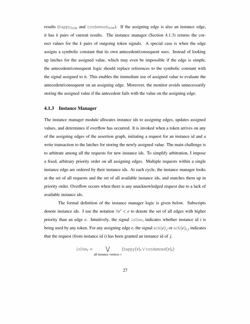
4.1.3 Instance Manager

The instance manager module allocates instance ids to assigning edges, updates assigned

values, and determines if overflow has occurred. It is invoked when a token arrives on any

of the assigning edges of the assertion graph, initiating a request for an instance id and a

write transaction to the latches for storing the newly assigned value. The main challenge is

to arbitrate among all the requests for new instance ids. To simplify arbitration, I impose

a fixed, arbitrary priority order on all assigning edges. Multiple requests within a single

instance edge are ordered by their instance ids. At each cycle, the instance manager looks

at the set of all requests and the set of all available instance ids, and matches them up in

priority order. Overflow occurs when there is any unacknowledged request due to a lack of

available instance ids.

The formal definition of the instance manager logic is given below. Subscripts

denote instance ids. I use the notation ∀e′ < e to denote the set of all edges with higher

priority than an edge e. Intuitively, the signal inUse i indicates whether instance id i is

being used by any token. For any assigning edge e, the signal ack(e) j or ack(e)i, j indicates

that the request (from instance id i) has been granted an instance id of j.

inUsei =_

all instance vertices v

(happy(v)i∨condemned(v)i)

27

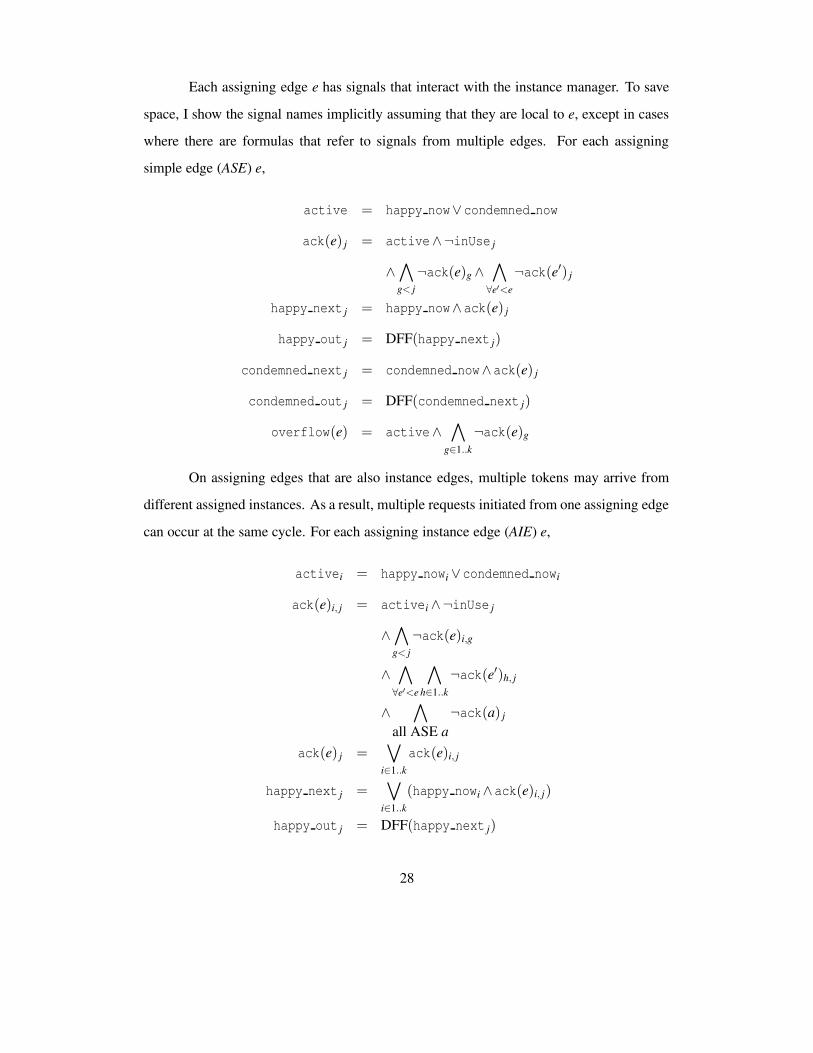
Each assigning edge e has signals that interact with the instance manager. To save

space, I show the signal names implicitly assuming that they are local to e, except in cases

where there are formulas that refer to signals from multiple edges. For each assigning

simple edge (ASE) e,

active = happy now∨condemned now

ack(e) j = active∧¬inUse j

∧^

g< j

¬ack(e)g∧^

∀e′<e

¬ack(e′) j

happy next j = happy now∧ack(e) j

happy out j = DFF(happy next j)

condemned next j = condemned now∧ack(e) j

condemned out j = DFF(condemned next j)

overflow(e) = active∧^

g∈1..k

¬ack(e)g

On assigning edges that are also instance edges, multiple tokens may arrive from

different assigned instances. As a result, multiple requests initiated from one assigning edge

can occur at the same cycle. For each assigning instance edge (AIE) e,

activei = happy nowi∨condemned nowi

ack(e)i, j = activei∧¬inUse j

∧^

g< j

¬ack(e)i,g

∧^

∀e′<e

^

h∈1..k

¬ack(e′)h, j

∧^

all ASE a¬ack(a) j

ack(e) j =_

i∈1..k

ack(e)i, j

happy next j =_

i∈1..k

(happy nowi∧ack(e)i, j)

happy out j = DFF(happy next j)

28

condemned next j =_

i∈1..k

(condemned nowi∧ack(e)i, j)

condemned out j = DFF(condemned next j)

overflow(e) =_

i∈1..k

(activei∧^

j∈1..k

¬ack(e)i, j)

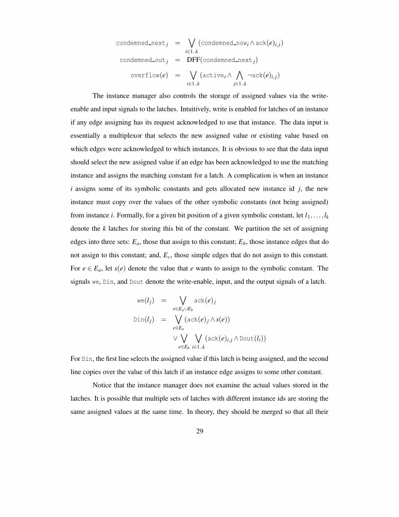
The instance manager also controls the storage of assigned values via the write-

enable and input signals to the latches. Intuitively, write is enabled for latches of an instance

if any edge assigning has its request acknowledged to use that instance. The data input is

essentially a multiplexor that selects the new assigned value or existing value based on

which edges were acknowledged to which instances. It is obvious to see that the data input

should select the new assigned value if an edge has been acknowledged to use the matching

instance and assigns the matching constant for a latch. A complication is when an instance

i assigns some of its symbolic constants and gets allocated new instance id j, the new

instance must copy over the values of the other symbolic constants (not being assigned)

from instance i. Formally, for a given bit position of a given symbolic constant, let l1, . . . , lk

denote the k latches for storing this bit of the constant. We partition the set of assigning

edges into three sets: Ea, those that assign to this constant; Eb, those instance edges that do

not assign to this constant; and, Ec, those simple edges that do not assign to this constant.

For e ∈ Ea, let s(e) denote the value that e wants to assign to the symbolic constant. The

signals we, Din, and Dout denote the write-enable, input, and the output signals of a latch.

we(l j) =_

e∈Ea∪Eb

ack(e) j

Din(l j) =_

e∈Ea

(ack(e) j ∧ s(e))

∨_

e∈Eb

_

i∈1..k

(ack(e)i, j ∧Dout(li))

For Din, the first line selects the assigned value if this latch is being assigned, and the second

line copies over the value of this latch if an instance edge assigns to some other constant.

Notice that the instance manager does not examine the actual values stored in the

latches. It is possible that multiple sets of latches with different instance ids are storing the

same assigned values at the same time. In theory, they should be merged so that all their

29

tokens carry the same instance id to free up memory resources. However, I felt that the

amount of hardware involved to compare values before every assignment is too complex

and not worth the savings it could achieve.

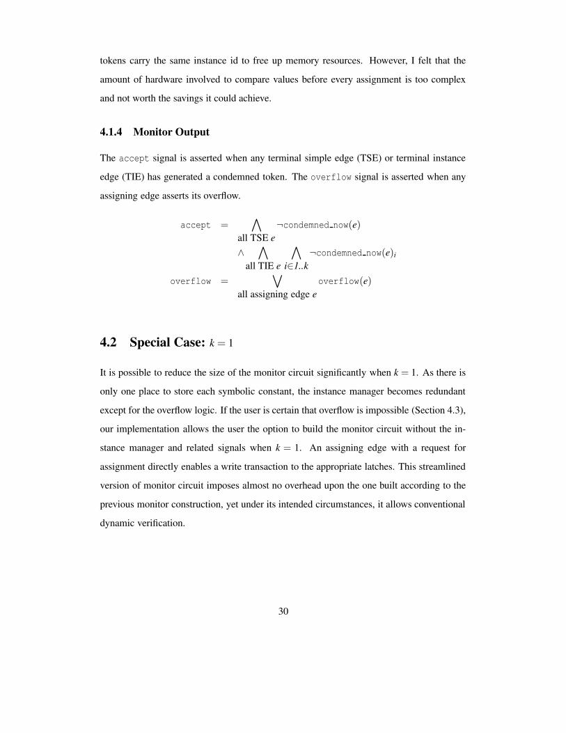
4.1.4 Monitor Output

The accept signal is asserted when any terminal simple edge (TSE) or terminal instance

edge (TIE) has generated a condemned token. The overflow signal is asserted when any

assigning edge asserts its overflow.

accept =^

all TSE e¬condemned now(e)

∧^

all TIE e

^

i∈1..k¬condemned now(e)i

overflow =_

all assigning edge eoverflow(e)

4.2 Special Case: k = 1

It is possible to reduce the size of the monitor circuit significantly when k = 1. As there is

only one place to store each symbolic constant, the instance manager becomes redundant

except for the overflow logic. If the user is certain that overflow is impossible (Section 4.3),

our implementation allows the user the option to build the monitor circuit without the in-

stance manager and related signals when k = 1. An assigning edge with a request for

assignment directly enables a write transaction to the appropriate latches. This streamlined

version of monitor circuit imposes almost no overhead upon the one built according to the

previous monitor construction, yet under its intended circumstances, it allows conventional

dynamic verification.

30

4.3 Bounding k

A natural question is what value of k should the user supply. I have observed that it is often

easy to determine an upper bound on the k that a given assertion graph requires.

A common special case is when, on all outgoing edges from each vertex, the an-

tecedents are mutually exclusive. In this case, the number of instances required is k = 1.

For example, the unpipelined adder example in Figure 2.4 in Chapter 2 obeys this constraint

and only needs k = 1, whereas the pipelined adder example does not obey this constraint

and requires k > 1. As noted in the preceding subsection, this is a very desirable special

case because the monitor circuit can be built with no overhead for instance management.

More generally, note that edges with assignment statements request a new instance

id every time they are active; we call these the requesting edges. If there is only one re-

questing edge in the assertion graph, the number of instances required is the same as the

maximum number of times that the edge receives a new token before a previously assigned

token is released. For example, returning to the pipelined adder in Chapter 2, Figure 2.6,

the edge from v0 to v1 is the requesting edge. If antecedent a0 is set correctly as ¬stall,

then the requesting edge can only receive three tokens (that aren’t immediately blessed)

during the lifetime of any token, so k = 3. On the other hand, if antecedent a0 is set to

be true, then an unbounded number of new tokens can pass through the requesting edge

while another token is stuck in a loop, so our analysis conservatively determines that k is

unbounded. If there are multiple requesting edges, the same analysis can be performed for

them individually, and the edges can be partitioned into groups where the lifetimes of the

assigned tokens by group members may overlap. The sum of required number of instances

of all group members is taken. The overall number of instances required for the assertion

graph is bounded by the largest sum amongst all the requesting edge groups.

31

Chapter 5

Experimental Results

In the last two chapters, I have introduced a new, simulation-friendly style of GSTE spec-

ifications and have presented a translation from simulation-friendly assertion graphs into

monitor circuits. Two natural questions are whether this new style of assertion graphs is

expressive enough and whether the new monitor construction is practical. Answering these

questions requires empirical evaluation using examples taken from real-life applications.

Although I do not have access to such examples, fortunately, Dr. Jin Yang from Intel’s

Strategic CAD Labs agreed to collaborate with me on this investigation. At Intel, engineers

have successfully applied GSTE in the verification of microprocessor designs. Due to con-

fidentiality issues, Dr Yang did not directly provide real examples of GSTE verification.

Instead, he graciously conducted experiments using Intel’s examples and the programs I

supplied.

I have created a software tool to generate monitor circuits for simulation-friendly

assertion graphs according to the construction described in Chapter 4. My programs are

written in FL, an interpreted, functional language, and are run using FORTE, a verification

system developed at Intel. A release of FORTE is freely available to the general public on

the Internet1 . I also intend to make my source code publicly available. The computer used

in the experiments was equipped with an Intel Pentium 4 processor running at 2.8 GHz.

1http://www.intel.com/software/productes/opensource/tools1/verification

32

Memory consumption was not an issue.

5.1 Simulation Friendliness in Real Life

To determine whether simulation-friendly assertion graphs are expressive enough for prac-

tical verification in real life, Dr. Yang selected 18 GSTE assertion graphs used in real, in-

dustrial verification. The 18 specifications cover various units in a microprocessor design,

ranging from memory to datapath to control intensive circuits and from the frontend to the

backend of the microarchitecture flow. Each of the specifications describes a non-trivial

functionality of a circuit. A majority of them cover the entire circuit from inputs to outputs.

The sizes of the circuits range from approximately 500 latches and 12,000 gates all the way

to around 45,000 latches and 240,000 gates. All the specifications have been verified using

GSTE model checking without any prior model abstraction/pruning.

Out of the 18 GSTE specifications, 15 are immediately convertible into the

simulation-friendly assertion graph format. (See Chapter 3 for details on the conversion.)

Manual effort is required for the actual conversion to ensure the meaning of the assertion

graphs is preserved during translation. The remaining 3 specifications include the use of

symbolic constants for symbolic indexing [12], which is not directly simulation-friendly.

However, all 3 specifications were still convertible with some extra manual effort. Specifi-

cally, typical usage of symbolic indexing is for case-splitting and for exploiting symmetry.

For case-splitting, the number of bits of symbolic index is small, so a symbolically-indexed

antecedent can be made simulation-friendly by duplicating the edge and enumerating the

cases. For symmetry, if there is an array of n presumed-symmetric storage locations (for

example, bits in a word, words in a memory, etc.), the symbolically-indexed assertion graph

uses log2 n bits of symbolic constant to index one of the n locations. There are two ways

to convert such assertion graphs into simulation-friendly format. The first is to generate n

instances of the edges with symbolic index, one for each possible value of the symbolic

index, exactly the same way as in handling case splitting. The second is to give up on sym-

metry and verify all n locations in a single instance. For example, if one is verifying a 64-bit

33

wide memory, there might be an antecedent like (din[63 : 0] = D[63 : 0]) without symbolic

indexing, or (din[K[5 : 0]] = D) with symbolic indexing, where D and K are symbolic

constants. In the former case, the antecedent is obviously simulation-friendly (by giving up

symmetry). In the latter case, one can make 64 copies of this edge for each possible value of

K, where the ith copy of the edge will have antecedent (K[5 : 0] = i)∧ (D = din[i]), which

is also simulation-friendly. In general, it may be possible to automate these conversions for

common usage idioms, but manual inspection is still suggested to ensure correctness. Over-

all, these results confirm my belief that simulation-friendly assertion graphs are expressive

enough for useful real-life applications.

5.2 Comparison with Previous Construction

The new monitor construction is based on the previous one [5], but it handles symbolic

constants correctly for conventional (non-symbolic) simulation. When symbolic simulation

is not available, the previous construction relies on the user to guess a single value for each

constant during initialization, which the monitor stores and uses to evaluate the whole trace.

Note that this does not capture GSTE semantics correctly. In my new construction, even

when a single value for each constant is stored (k = 1), the monitor correctly stores the

assigned value and asserts the overflow signal when overflow occurs. The cost of this

improvement should be increased circuit complexity, but I believe that the new monitors

should remain practical in terms of size. Furthermore, I expect the new construction to

behave similarly to the previous one in terms of its linear scaling trend with increasing size

of the assertion graph.

To test these hypotheses, we have run experiments to compare three different mon-

itor constructions: Previous, Light, and Full. Previous is exactly the one used in the prior

work. Both Light and Full are new constructions for simulation-friendly assertion graphs,

both with k = 1. Light differs from Full in that it does not have an overflow signal and

the associated logic. (See Section 4.2 for more details on the differences between Light and

Full.) We used the same assertion graph examples from the previous paper [5] and ran sim-

34

ilar experiments. There are two families of assertion graphs. One describes a property of a

memory unit, where the width of the address lines can be varied. A wider address means the

antecedents and consequents involve more signals and are thus more complicated. Another

family of assertion graphs describes a property of a FIFO, where the depth can be changed.

A deeper FIFO means a larger assertion graph with more edges and vertices.

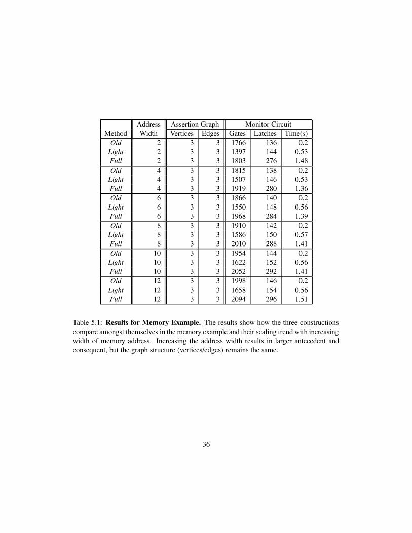
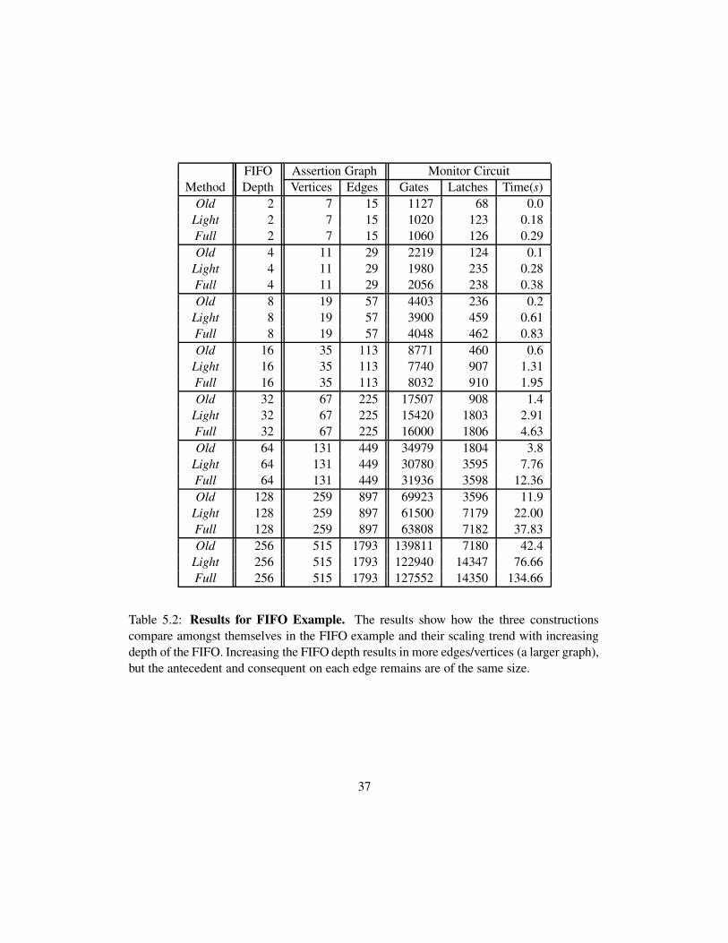
Table 5.1 and Table 5.2 contains the results of the experiments. As a pleasant sur-

prise, Light produced the smallest monitors in all cases, and Full also generated smaller

monitors than Previous in the FIFO depth family, despite the overhead of the instance man-

ager module. The reason is that there is a significant reduction in circuit size after removing

the logic for antecedents, which became assignment statements in the simulation-friendly

format. Even in cases where Full produced larger monitors, the difference is in the range

of 10-20%. In terms of scaling, the monitors generated by the new constructions behave

similarly to those by previous one. They scale linearly with both the assertion graph size

and the antecedent/consequent size. Figure 5.1 and Figure 5.2 illustrates the scaling trend

by plotting the results.

5.3 Effect of Changing the Parameter k

It is obvious from examining the translation that most of the monitor should scale linearly

with the value of k as well. For the subcircuits that depend on k, the construction generates

k copies of the signals and their associated logic. Other subcircuits may be unaffected by a

changing k. Only the instance manager has some logic that is O(k2) in order to find the free

instances. Experimental results confirm that the small O(k2) term is dominated in practice

for small k, so the observed growth is linear. The run time of monitor generation also scaled

linearly with k. Figure 5.3 shows the scaling of monitor size with k for several assertion

graph example runs.

35

Address Assertion Graph Monitor CircuitMethod Width Vertices Edges Gates Latches Time(s)

Old 2 3 3 1766 136 0.2Light 2 3 3 1397 144 0.53Full 2 3 3 1803 276 1.48Old 4 3 3 1815 138 0.2

Light 4 3 3 1507 146 0.53Full 4 3 3 1919 280 1.36Old 6 3 3 1866 140 0.2

Light 6 3 3 1550 148 0.56Full 6 3 3 1968 284 1.39Old 8 3 3 1910 142 0.2

Light 8 3 3 1586 150 0.57Full 8 3 3 2010 288 1.41Old 10 3 3 1954 144 0.2

Light 10 3 3 1622 152 0.56Full 10 3 3 2052 292 1.41Old 12 3 3 1998 146 0.2

Light 12 3 3 1658 154 0.56Full 12 3 3 2094 296 1.51

Table 5.1: Results for Memory Example. The results show how the three constructionscompare amongst themselves in the memory example and their scaling trend with increasingwidth of memory address. Increasing the address width results in larger antecedent andconsequent, but the graph structure (vertices/edges) remains the same.

36

FIFO Assertion Graph Monitor CircuitMethod Depth Vertices Edges Gates Latches Time(s)

Old 2 7 15 1127 68 0.0Light 2 7 15 1020 123 0.18Full 2 7 15 1060 126 0.29Old 4 11 29 2219 124 0.1

Light 4 11 29 1980 235 0.28Full 4 11 29 2056 238 0.38Old 8 19 57 4403 236 0.2

Light 8 19 57 3900 459 0.61Full 8 19 57 4048 462 0.83Old 16 35 113 8771 460 0.6

Light 16 35 113 7740 907 1.31Full 16 35 113 8032 910 1.95Old 32 67 225 17507 908 1.4

Light 32 67 225 15420 1803 2.91Full 32 67 225 16000 1806 4.63Old 64 131 449 34979 1804 3.8

Light 64 131 449 30780 3595 7.76Full 64 131 449 31936 3598 12.36Old 128 259 897 69923 3596 11.9

Light 128 259 897 61500 7179 22.00Full 128 259 897 63808 7182 37.83Old 256 515 1793 139811 7180 42.4

Light 256 515 1793 122940 14347 76.66Full 256 515 1793 127552 14350 134.66

Table 5.2: Results for FIFO Example. The results show how the three constructionscompare amongst themselves in the FIFO example and their scaling trend with increasingdepth of the FIFO. Increasing the FIFO depth results in more edges/vertices (a larger graph),but the antecedent and consequent on each edge remains are of the same size.

37

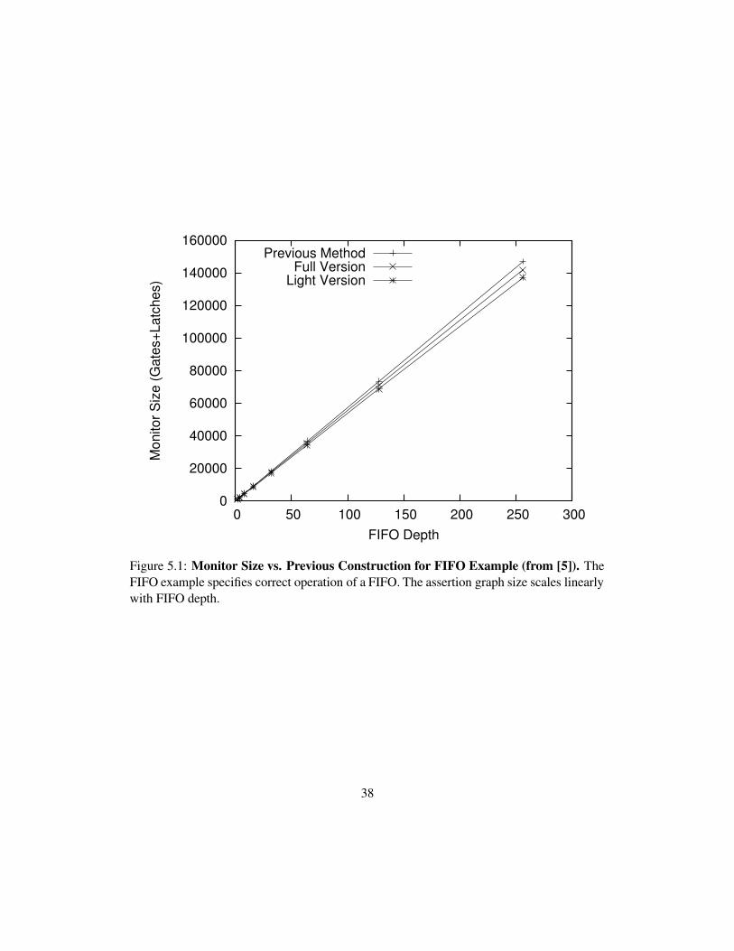
0

20000

40000

60000

80000

100000

120000

140000

160000

0 50 100 150 200 250 300

Mon

itor S

ize

(Gat

es+L

atch

es)

FIFO Depth

Previous MethodFull Version

Light Version

Figure 5.1: Monitor Size vs. Previous Construction for FIFO Example (from [5]). TheFIFO example specifies correct operation of a FIFO. The assertion graph size scales linearlywith FIFO depth.

38

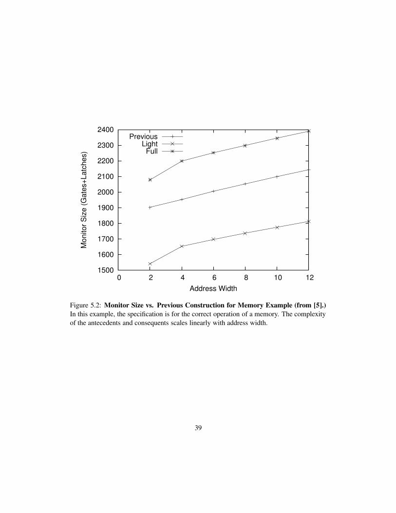
1500

1600

1700

1800

1900

2000

2100

2200

2300

2400

0 2 4 6 8 10 12

Mon

itor S

ize

(Gat

es+L

atch

es)

Address Width

PreviousLight

Full

Figure 5.2: Monitor Size vs. Previous Construction for Memory Example (from [5].)In this example, the specification is for the correct operation of a memory. The complexityof the antecedents and consequents scales linearly with address width.

39

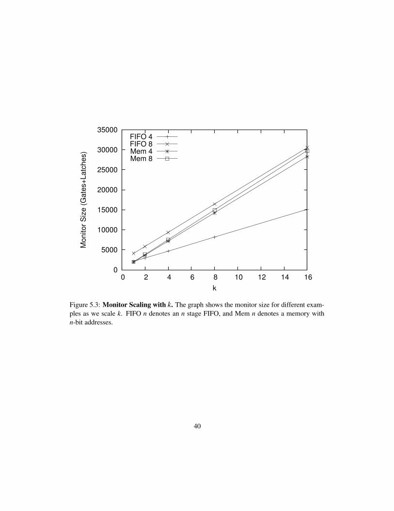
0

5000

10000

15000

20000

25000

30000

35000

0 2 4 6 8 10 12 14 16

Mon

itor S

ize

(Gat

es+L

atch

es)

k

FIFO 4FIFO 8Mem 4Mem 8

Figure 5.3: Monitor Scaling with k. The graph shows the monitor size for different exam-ples as we scale k. FIFO n denotes an n stage FIFO, and Mem n denotes a memory withn-bit addresses.

40

5.4 Real Industrial Example

We have applied the new monitor construction to a real, industrial example. It is also the

same example used in the previous paper [5], but with some modifications to make the

assertion graph simulation-friendly. The industrial circuit is large, containing 403972 gates

and 35157 latches. The new simulation-friendly monitor is run to watch a 25000 cycle

random trace. In the previous paper, the authors reported a slowdown of 16% when the

previous monitor circuit was added to simulation. In my experiment, the baseline run time

was 1680.18s with the circuit under verification only. The run time with monitor (k = 1) was

1737.69s, a 3.4% slowdown. This is expected because the burden of symbolic simulation

has been lifted. The result confirmed my belief that simulation-friendly assertion graphs

and their monitor construction are indeed practical for real industrial usage.

41

Chapter 6

Testbench Generation

A circuit performs its function by interacting with the outside world through its input/output

interface. The correctness of a system cannot be determined until both the input and the out-

put are known. A simulation/emulation run is possible only when there is a model of the

environment in addition to that of the system. The environment interacts with the system

under verification by supplying input vectors or stimuli, enabling engineers to observe sys-

tem behaviour. The environment is usually modelled by a testbench, which contains input

sequences created by engineer to exercise interesting scenarios while obeying a specific set

of rules. Those rules are called input constraints, which defines the legal input space; de-

signers of a system can and often assume that input constraints are always satisfied. Input

constraints are functions of the interface signals that involve both the environment and the

system.

To create quality testbenches for modern industrial designs is challenging. Not only

does the input space grow with circuit size and complexity, the number of input constraints

also increases, and their complexity as well. Researchers have proposed automation as an

answer. If the user clearly defines the constraints, tools have been created to generate input

automatically during verification. Additionally, some tools allow the user to direct (bias)

towards certain input values, subject to the constraints being satisfied. Previous work [16,

24, 4, 22, 23] focused on creating software for input generation, and the constraints are

42

written in different styles. There has been no attempt to create a testbench generation tool

for constraints written as GSTE properties, which would be a step to bridge the gap between

GSTE-style formal verification and dynamic verification.

I investigated the topic of constructing a testbench generator from input constraints

specified as a GSTE assertion graph. GSTE allows users to write properties that express

temporal relations between signals, which should suffice for representing input constraints.

Constructing a testbench generator also requires the definition of the environment, the set

of input signals of the system under verification. Instead of going in the same direction as

other researchers, I explored building a hardware tool, a testbench generator circuit. My

idea is to build on top of my work described in the previous chapters.

I saw a connection between a monitor circuit and a testbench generator. Given an as-

sertion graph that expresses input constraints of the system under verification, I have shown

in Chapter 4 how to build a monitor circuit that determines whether the input constraints

are satisfied. The monitor circuit asserts its accept signal only when the constraints are

satisfied. Further examination reveals that the logic behind this signal is a function of rele-

vant signals of the system and latches of the monitor. At each cycle, the values of relevant

system signals and monitor latches uniquely determine the value of accept. A natural way

to build a testbench generator is, therefore, to build a circuit that output environment signal

values that always ensure that the accept signal remains asserted at every cycle. In other

words, given access to values of relevant monitor latches and system signals, the testbench

generator solves for an assignment to the environment signals that guarantees the accept

function is satisfied. This implies that either the testbench generator is always used together

with a monitor, or it has a module that is essentially a built-in monitor.

Different methods exist to solve for assignments of boolean functions, but I needed

one that can easily be implemented in hardware. For this reason, I have chosen to construct

a binary decision diagram (BDD) for the accept function. Kukula and Shiple [9] presented

a method to translate a free BDD into a circuit. (An ordinary BDD is just a special case

of a free BDD.) Some of the BDD variables are identified as input and others as output

43

of the circuit. The circuit has auxiliary inputs to resolve the case where both values (0

and 1) of an output variable are possible. The circuit returns the values of output variables

that will satisfy its BDD function given the values of the input variables. The translated

circuit is structured according to the BDD, and hence its size depends directly and linearly

on the number of BDD nodes. While BDD size depends on many factors, generally, if the

number of variables is small and the function is not too complex, the number of BDD nodes

should be manageable during and after BDD construction. Furthermore, the complexity of

the accept logic depends only on the assertion graph, mostly the antecedents/consequents,

and not the system under verification. Therefore, BDD blowup should not be a problem for

this method.

I implemented the above idea into a program written in FL. Although the resulting

testbench generators function correctly — that is, input constraints are satisfied — the input

sequences generated do not make useful testbenches for practical verification, because the

input sequences do not lead to scenarios that are important to verifying the system. In

other words, the coverage is inadequate. For example, one rule may read, “if the request

was asserted in the previous cycle, the acknowledgment must be asserted in the current

cycle.” The testbench generator may generate sequences that never exercise this scenario,

yet they satisfy the constraint vacuously. In theory, controlling the auxiliary inputs can

improve coverage, but it is not clear how better coverage can be achieved given the limited

amount of information. One apparent solution is to direct the testbench generator to satisfy

as many of the antecedents as possible. Aside from technical difficulties it may involve,

there is a philosophical question. A single property can be written in two ways, which give

rise to totally reversed set of antecedents and consequents. In the same example above,

another user may write that, “if the acknowledgement is not asserted in the current cycle,

then the request was not asserted in the previous cycle.” This same description specifies

exactly the same property, but the antecedent and consequent are reversed. It is not at all

clear whether the tool should infer different intents for two assertion graphs with the same

formal semantics.

44

The proposed setup of building testbench generators upon the success of the monitor

circuit construction has not produced favourable results. Due to time constraints, I have

decided that further investigation is beyond the scope of my research at this point. I expect,

however, researchers to conduct future work on this topic, as it is of significant interest from

the industry.

45

Chapter 7

Conclusions and Future Work

In this thesis, I have introduced a novel, simulation-friendly style of GSTE assertion graphs.

I have also presented a method to construct monitor circuits for such assertion graphs.

The constructed monitor circuits correctly handle symbolic constants and work under con-

ventional dynamic verification without symbolic simulation. Combined with my straight-

forward translation from simulation-friendly assertion graphs into conventional assertion

graphs, my work allows using the same specification with both formal GSTE model check-

ing as well as dynamic verification. Empirical results show that simulation-friendly asser-

tion graphs are expressive enough for real, industrial usage, and that the monitor circuit

generation is efficient, scaling linearly with assertion graph size and the number of in-

stances needed. This work is an important step towards seamlessly integrating formal and

dynamic verification. I have also done preliminary investigation into generating testbenches

for GSTE assertion graphs.

Future work include improvements to both monitor circuit construction and test-

bench generation. Currently, an assignment statement is only allowed to assign a single

system signal to a symbolic constant. Future version of the work should expand to allow

greater flexibility, such as allowing the assignment of arithmetic/logical expressions to sym-

bolic constants, and the expressions may even contain other assigned symbolic constants.

One further step is to consider the possibility of assigning multiple values to the same

46

constant at a time, but this would involve significant modification of the instance manager

module. Also, it may be worth considering whether there is an efficient means of avoiding

storing identical assignments in different active instances of a monitor circuit. Automatic

determination of the value of k that guarantees no overflow would be a useful feature. It

would allow a further reduction of the monitor size by eliminating the overflow logic.

On the problem of testbench generation for GSTE, my research was only a start and

a lot of future work is needed. My initial findings suggest that using a GSTE monitor circuit

as the basis to construct a testbench generator circuit will not produce adequate coverage.

I have also shown targeting the satisfaction of antecedents is not always a good heuris-

tic for better coverage. I believe future work on this subject will move towards building

and improving software that executes in parallel with a simulator to generate high-quality

verification sequences.

47

Bibliography

[1] Lionel Bening and Harry Foster. Principles of Verifiable RTL Design: A Functional

Coding Style Supporting Verification Processes in Verilog. Kluwer Academic Pub-

lishers, 2nd edition, 2001.

[2] Bob Bentley. High level validation of next generation microprocessors. In Interna-

tional Workshop on High-Level Design, Validation, and Test. IEEE, 2002.

[3] Edmund M. Clarke and E. Allen Emerson. Design and synthesis of synchronization

skeletons using branching time temporal logic. In Dexter Kozen, editor, Workshop on

Logics of Programs, pages 52–71, May 1981. Published 1982 as Lecture Notes in

Computer Science Number 131.

[4] Pei-Hsin Ho, Thomas Shiple, Kevin Harer, James Kukula, Robert Damiano, Valeria

Baertacco, Jerry Taylor, and Jiang Long. Smart simulation using collaborative for-

mal and simulation engines. In International Conference on Computer-Aided Design,

pages 120–126. ACM/IEEE, 2000.

[5] Alan J. Hu, Jeremy Casas, and Jin Yang. Efficient generation of monitor circuits

for GSTE assertion graphs. In International Conference on Computer-Aided Design,

pages 154–159. IEEE/ACM, 2003.

[6] Alan J. Hu, Jeremy Casas, and Jin Yang. Reasoning about GSTE assertion graphs. In

Correct Hardware Design and Verification Methods: 12th IFIP WG 10.5 Advanced

48

Research Working Conference (CHARME’03), pages 170–184. Springer, 2003. Lec-

ture Notes in Computer Science Number 2860.

[7] M. S. Jahanpour and E. Cerny. Compositional verification of an ATM switch mod-

ule using interface recognizer/suppliers (IRS). In International High-Level Design,

Validation, and Test Workshop, pages 71–76. IEEE, 2000.

[8] Matt Kaufmann, Andrew Martin, and Carl Pixley. Design constraints in symbolic

model checking. In Computer-Aided Verification: 10th International Conference,

pages 477–487. Springer, 1998. Lecture Notes in Computer Science Number 1427.

[9] James H. Kukula and Thomas R Shiple. Building circuits from relations. In 12th

International Conference on Computer Aided Verification, pages 113–123. Springer-

Verlag, 2000. Lecture Notes in Computer Science Number 1855.

[10] Robert P. Kurshan. Computer-Aided Verification of Coordinating Processes: The

Automata-Theoretic Approach. Princeton University Press, 1994.

[11] Zohar Manna and Amir Pnueli. Specification and verification of concurrent programs

by ∀-automata. In Symposium on Principles of Programming Languages, pages 1–12.

ACM, 1987.

[12] Thomas F. Melham and Robert B. Jones. Abstraction by symbolic indexing trans-

formations. In Formal Methods in Computer-Aided Design: Fourth International

Conference, pages 1–18. Springer, 2002. Lecture Notes in Computer Science Num-

ber 2517.

[13] Jean-Pierre Queille and Joseph Sifakis. Specification and verification of concurrent

systems in Cesar. In 5th International Symposium on Programming, pages 337–351.

Springer, 1981. Lecture Notes in Computer Science Number 137.

[14] Roberto Sebastiani, Eli Singerman, Stefano Tonetta, and Moshe Y. Vardi. GSTE is

partitioned model checking. In Computer-Aided Verification: 16th International Con-

49

ference. Springer-Verlag, 2004. Lecture Notes in Computer Science Number. To ap-

pear.

[15] Carl-Johan H. Seger and Randal E. Bryant. Formal verification by symbolic evaluation

of partially-ordered trajectories. Formal Methods in System Design, 6(2):147–190,

1995.

[16] Kanna Shimizu and David L. Dill. Deriving a simulation input generator and a cover-

age metric from a formal specification. In 39th Design Automation Conference, pages

801–806. ACM/IEEE, 2002.

[17] Kanna Shimizu, David L. Dill, and Alan J. Hu. Monitor-based formal specification of

PCI. In Formal Methods in Computer-Aided Design, pages 335–353. Springer, 2000.

Lecture Notes in Computer Science Number 1954.

[18] Moshe Y. Vardi and Pierre Wolper. An automata-theoretic approach to automatic

program verification. In Symposium on Logic in Computer Science, pages 332–344.

IEEE Computer Society, 1986.

[19] Jin Yang and Amit Goel. GSTE through a case study. In International Conference on

Computer-Aided Design, pages 534–541. IEEE/ACM, 2002.

[20] Jin Yang and Carl-Johan H. Seger. Introduction to generalized symbolic trajectory

evaluation. In International Conference on Computer Design, pages 360–365. IEEE,

2001.

[21] Jin Yang and Carl-Johan H. Seger. Generalized symbolic trajectory evaluation —

abstraction in action. In Formal Methods in Computer-Aided Design: Fourth Interna-

tional Conference, pages 70–87. Springer, 2002. Lecture Notes in Computer Science

Number 2517.

[22] Jun Yuan, Ken Albin, Adnan Aziz, and Carl Pixley. Constraint synthesis for environ-

mental modeling in functional verification. In 40th Design Automation Conference,

pages 296–299. ACM/IEEE, 2003.

50

[23] Jun Yuan, Carl Pixley, Adnan Aziz, and Ken Albin. A framework for constrained

functional verification. In International Conference on Computer-Aided Design, pages

142–145. ACM/IEEE, 2003.

[24] Jun Yuan, Kurt Shultz, Carl Pixley, Hillel Miller, and Adnan Aziz. Modeling design

constraints and biasing in simulation using BDDs. In International Conference on

Computer-Aided Design, pages 584–589. IEEE/ACM, 1999.

51