REVIEW

COPY

NOT FOR D

ISTRIB

UTION

Femtosecond-pulsed optical heating of gold nanoparticles

Guillaume Baffou∗ and Herve RigneaultInstitut Fresnel, CNRS, Aix-Marseille Universite, Ecole Centrale de Marseille,

Domaine Universitaire Saint-Jerome, 13397 Marseille, France

(Dated: March 10, 2011)

We investigate theoretically and numerically the thermodynamics of gold nanoparticles immersedin water and illuminated by a femtosecond-pulsed laser at their plasmonic resonance. The spatio-temporal evolution of the temperature profile inside and outside is computed using a numericalframework based on a Runge-Kutta algorithm of the fourth order. The aim is to provide a com-prehensive description of the physics of heat release of plasmonic nanoparticles under pulsed illu-mination, along with a simple and powerful numerical algorithm. In particular, we investigate theamplitude of the initial instantaneous temperature increase, the physical differences between pulsedand cw illuminations, the time scales governing the heat release into the surroundings, the spatialextension of the temperature distribution in the surrounding medium, the influence of a finite ther-mal conductivity of the gold/water interface, the influence of the pulse repetition rate of the laser,the validity of the uniform temperature approximation in the metal nanoparticle, and the optimumnanoparticle size (around 40nm) to achieve maximum temperature increase.

I. INTRODUCTION

Gold nanoparticles (NPs) can act as efficient nano-sources of heat under visible or infrared illuminationat the plasmonic resonance due to enhanced lightabsorption.1 The ability to locally heat at the nanoscaleopens the path for new promising achievements inNanotechnology and especially for nanoscale control oftemperature distribution,2 chemical reactions,3 phasetransition,4 material growth,5 photothermal cancertherapy6–8 and drug release.9,10

The use of femtosecond-pulsed illumination on goldNPs expands the range of applications compared to con-tinuous (cw) illumination. First, it can lead to non-linear optical processes like two-photon luminescence orsecond harmonic generation with applications mainly inbio-imaging.11,12 Then, it can trigger a sudden tempera-ture increase at the sub-nanosecond scale and subsequenteffects such as acoustic waves used for opto-acousticimaging13,14 or bubble formation for nanosurgery.15 Asharp and brief temperature increase of a NP generatedby a femtosecond laser can also contribute to confine thetemperature increase at the close vicinity of the NP toavoid extended heating of the whole medium when notdesired.16

Several experimental and numerical approaches aimedat studying the internal processes of heat genera-tion under pulsed illumination and the subsequent ef-fects observed in the surrounding medium, e.g. tem-perature and pressure variations,17–19 acoustic wavegeneration,18 vibration modes,20–22, cell apoptosis,11

drug release9,23 nanosurgery,15,24 bubble formation,25–28

NP shape modification29 and melting,29–31 nanosecond-pulses for biomedical applications,32,33 extreme thermo-dynamics conditions.33–37

In this paper, we present and use a versatile numer-ical framework to investigate theoretically and numeri-cally the evolution of the temperature distribution of agold nanoparticle immersed in water when shined by afemtosecond-pulsed laser. Various degrees of complexityexist to describe theoretically such a problem. We chosea progressive approach consisting in going from simpleto more sophisticated: We shall start with the more ba-

sic description of the problem, a point-like source of heatto model the NP, and then refine the description of thesystem by taking into account successive refinements,namely a finite-size structure, an gold/water interfaceconductivity and a non-uniform NP inner temperature.In each case, the physics and the associated constitutiveequations are detailed and the approximations discussed.The aim is to answer all the questions related to charac-teristic time, space and temperature increase in fs-pulsedoptical heating of gold NP.Details regarding the numerical algorithm we devel-

oped are given in appendix.

II. RESULTS AND DISCUSSION

A. Physical system

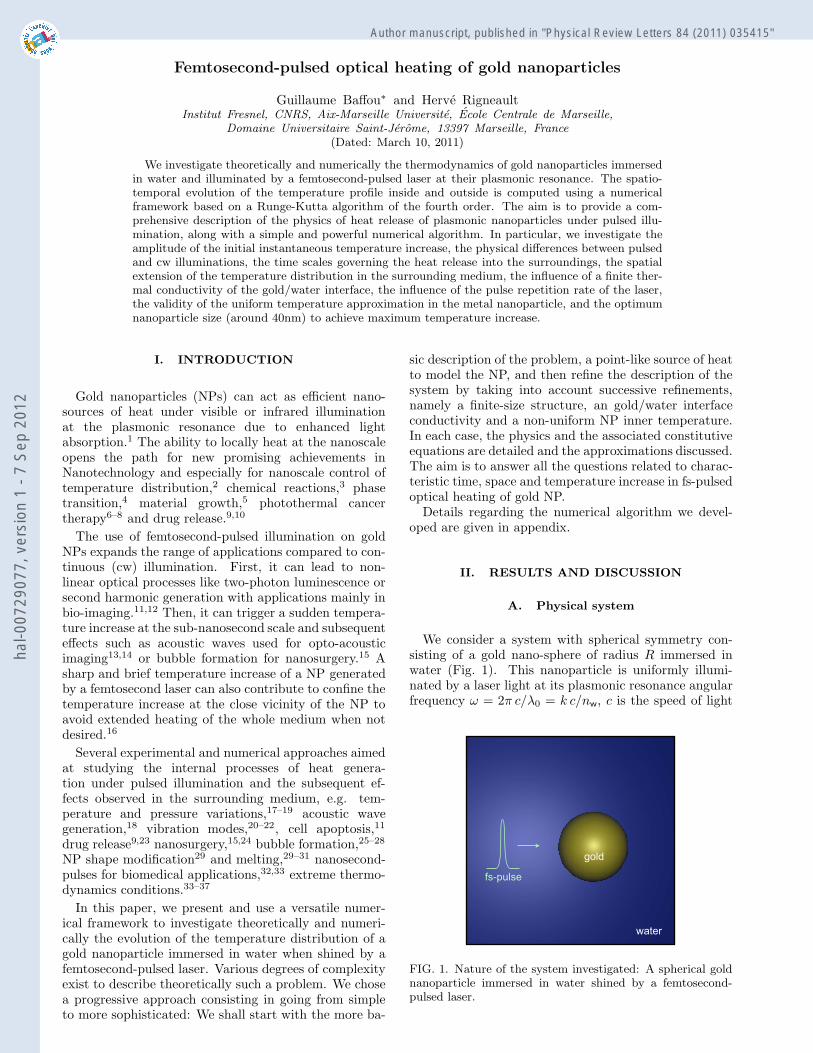
We consider a system with spherical symmetry con-sisting of a gold nano-sphere of radius R immersed inwater (Fig. 1). This nanoparticle is uniformly illumi-nated by a laser light at its plasmonic resonance angularfrequency ω = 2π c/λ0 = k c/nw, c is the speed of light

water

gold

fs-pulse

FIG. 1. Nature of the system investigated: A spherical goldnanoparticle immersed in water shined by a femtosecond-pulsed laser.

hal-0

0729

077,

ver

sion

1 -

7 Se

p 20

12Author manuscript, published in "Physical Review Letters 84 (2011) 035415"

2

and nw the optical index of water. No mass transfer likefluid convection or bubble formation is considered. Weshall focus on moderate temperature increase (typicallya few tens of degrees) and not consider extreme thermo-dynamic conditions. For this reason, all the parametersdescribing the materials (water and gold) are assumedto remain constant within the temperature range inves-tigated. Whenever a femtosecond pulse is mentioned, ithas to be understood as a pulse, the duration of which issmaller than the characteristic time of electron–phononscattering τe−ph ∼ 1.7 ps. For instance, this can corre-spond to the use of a Ti:Sapphire laser, which usuallyprovides a pulse duration around 100 fs.In the following, any mentioned temperature T will

have to be understood as a temperature increase abovethis initial ambient temperature.Anywhere in the system, we can define the ther-

mal energy density and thermal current density thatread respectively uth(r, t) = ρ c T (r, t) and jth(r, t) =−κ∇T (r, t) where ρ is the mass density, c the specificheat capacity at constant pressure and κ the thermalconductivity of the system at the position r. From theenergy conservation equation ∂tuth(r, t) +∇ · jth(r, t) =p(r, t), on obtain the heat diffusion equation:

ρ c ∂tT (r, t) = κ∇2T (r, t) + p(r, t) (1)

where p(r, t) is the heat power density (nonzero only in-side the NP (r < R), where the light is absorbed),For the system under consideration in this work, this

yields a set of two differential equations, one for eachmedium (gold and water), along with two boundary con-ditions at the gold/water interface:

Diffusion equations:

ρAu cAu ∂tT (r, t) = κAu∇2T (r, t) + p(r, t) for r < R

ρw cw ∂tT (r, t) = κw∇2T (r, t) for r > R

Boundary conditions at r = R:

κw∂rT (R+, t) = κAu∂rT (R

−, t)

T (R+, t) = T (R−, t)

(2)

Au and w subscripts refer to gold and water. The firstboundary condition ensures heat flux conservation at theNP interface.It has been demonstrated experimentally that an in-

terface resistivity at the gold/water interface exists andcan play a significant role in the heat release.38–41 The in-terface resistivity can reach appreciable values when theliquid does not wet the solid. The wetting depends onthe nature of the interface, and in particular a possiblemolecular coating. Namely, hydrophobic coatings areassociated to poor thermal conductivities. The directconsequence of a finite interface conductivity g (or re-sistivity 1/g) is a temperature drop/jump/discontinuity∆T at the NP interface such as:

P(t) = 4πR2 g∆T (t) (3)

where ∆T is defined such as:

∆T (t) ≡ T (R−, t)− T (R+, t) (4)

(in this work, the symbol ≡ symbolizes a definition).The released heat power P(t) is also related to the tem-perature gradient on the NP surface through the energy

conservation equation:

P(t) = −4πR2 κw ∂rT (R, t). (5)

Equations (3) and (5) yield a modification of the secondboundary condition of system (2) at the nanoparticleinterface r = R:

−∂r T (R+, t) =1

lK∆T (t) (6)

where lK = κw/g is named the Kapitza length and 1/gis the associated Kapitza resistivity.

Let us define from now two dimensionless constantsthat we shall often use in the following,

β ≡ ρwcwρAucAu

≈ 1.680 (7)

γ ≡ κAuκw

≈ 512 (8)

and one dimensionless parameter:

λK ≡ κwg R

=lKR

(9)

that is the Kaptiza length normalized by the NP radiusR. We also introduce dimensionless space ρ and time τvariables defined such as:

ρ ≡ r/R (10)

τ ≡ awt/R2 (11)

where a = κ/ρc is called the thermal diffusivity. R andR2/aw are indeed the natural space and time units asso-ciated to the system. Within this work, we will make anextensive use of dimensionless variables and constants,first because it yields simpler, more natural formulae andmore general results, and then because it shows how thealgorithm can be properly written, i.e. working withnumbers close to one and not unnecessary powers of ten.However, for the sake of simplicity, even when using nor-malized variables, we shall keep the same function names– e.g. T (r, t) and T (ρ, τ). But this mathematical digres-sion should not cause any clarity issue.Using these dimensionless variables, parameters and

constants, the set of equations (2) along with the addi-tional boundary condition (6) read then:

Diffusion equations:

∂τT (ρ, τ) =γ β

ρ2∂ρ

(

ρ2∂ρT (ρ, τ))

+ p(ρ, τ) for ρ < 1

∂τT (ρ, τ) =1

ρ2∂ρ

(

ρ2∂ρT (ρ, τ))

for ρ > 1

Boundary conditions at ρ = 1:

∂ρT (1+, τ) = γ ∂ρT (1

−, τ) = − 1

λK∆T (τ)

(12)

where the Laplacian operator ∇2 has been reformulatedusing spherical coordinates.From now on, the use of dimensionless formalism will

not be systematic, but preferred when it simplifies thenotations and make the results more general.

hal-0

0729

077,

ver

sion

1 -

7 Se

p 20

12

3

TABLE I. Physical constants used in this work associated togold and water.a.

Name Gold Water UnitThermal conductivity κ 317 0.60 W/m/KSpecific heat capacityb c 129 4187 J/kg/KMass density ρ 19.32 1.00 ×103 kg/m3

Thermal diffusivity a 127 0.143 ×10−6 m2/s

a Values at approx. 25◦C taken from ref. [42]b at constant pressure

B. Numerical method

The set of equations (12) has no simple analytical solu-tion. We chose to solve it numerically by developing a fi-nite difference method (FDM) and a Runge-Kutta (RK)algorithm.43 Basically, it is based on a spatio-temporaldiscretization of the system of equations (12) accordingto:

ρi ≡ i× δρ i ∈ [0, N ]

τj ≡ j × δτ j ∈ [0,M ]

Ti,j ≡ T (ρi, τj)

∂ρT (ρ, τ) →Ti+1,j − Ti,j

δρ

∂τT (ρ, τ) →Ti,j+1 − Ti,j

δτ.

(13)

This discretization procedure is associated with a RK al-gorithm of the fourth order (RK4) that ensures a higheraccuracy – compared to regular Euler algorithms of thefirst order – in the estimation of Ti,j at each spatio-temporal step.Further details regarding the numerical algorithm are

given in the appendix.

C. cw illumination

Before studying what occurs under femtosecond (fs)pulsed illumination, it is worth describing first what hap-pens under continuous (cw) illumination. We consider inthis paragraph a uniform cw illumination of irradiance Iand wavelength λ0.Under cw illumination, the establishment of the steady

state temperature profile will be preceded by a transientevolution. By dimensional analysis of the two diffusionequations of system (2), one find that two time scalescome into play:

τwd =ρw cwκw

R2 =R2

aw, (14)

τAud =ρAu cAuκAu

R2 =R2

aAu. (15)

τwd is the characteristic time associated to the evolutionof the temperature profile in the surrounding water whileτAud characterizes the temperature evolution inside thegold NP. Since aAu ≫ aw, the thermalization inside theNP occurs much faster. Consequently, one can consider

that the global establishment of the temperature pro-file of the overall system is governed by the time scale τwd .

We consider now the final steady state regime. Theset of equations reads now:

κAu∇2T (r) = −p(r) for r < R

κw∇2T (r) = 0 for r > R

κw∂rT (R+) = κAu∂rT (R

−)

= −g∆T

(16)

where ∆T ≡ T (R−)−T (R+). If one consider an averagepower density p0 = P0/V , the solution has a simple formand reads:

T cw(r) =P0

4π κw rfor r > R (17)

T cw(r) =P0

4π κwR

[

1 +1

2γ

(

1− r2

R2

)

+ λK

]

for r < R

(18)

where P0 is the heat power dissipated in the NP. Notethat the temperature profile outside the NP does notdepend on the NP surface conductivity.44 Since γ ≫ 1,one can usually consider – whatever the NP size – thatthe inner temperature of the NP is uniform and equals:

T cwNP =

P0

4π κwR(1 + λK) =

σabs I

4π κwR(1 + λK) (19)

where σabs is the optical absorption cross section of theNP.2,45 For spherical nanoparticle smaller than 2R ∼ 30nm, a good approximation can be used:46

σabs = k Im(α) − k4

6π|α|2 (20)

where α =α0

1− (2/3)ik3α0(21)

and α0 = 4π R3 εAu − εwεAu + 2 εw

(22)

with εAu the gold permittivity and εw the water permit-tivity.From equation (19), we obtain thus a simple and very

useful formula that gives the steady-state temperature ofsmall spherical NP (R < 15 nm) under cw illumination:

T cwNP =

k I R2

κwIm

(

εAu − εwεAu + 2 εw

)

, (23)

T cwNP ≈ 2.00× k I R2

κw. (24)

The latter formula applies for λ0 = 520 nm. No interfaceresistivity is assumed in this formula (λK = 0). If theNP is not necessarily smaller than 2R = 30 nm, theprevious formalism becomes inappropriate and the moresophisticated and general Mie theory has to be used.46

Within this model, the absorption cross section reads:

σabs =2π

k2

∞∑

j=1

(2j + 1) (|aj |2 + |bj |2)

where

aj =mψj(v)ψ

′

j(u) − ψj(u)ψ′

j(v)

mψj(v) ξ′j(u) − ξj(u)ψ′

j(v),

bj =ψj(v)ψ

′

j(u) − mψj(u)ψ′

j(v)

ψj(v) ξ′j(u) − mξj(u)ψ′

j(v)

hal-0

0729

077,

ver

sion

1 -

7 Se

p 20

12

4

and m2 = εAu/εw, u = kR and v = mu. The primesindicates differentiation with respect to the argumentin parenthesis. ψj and ξj are Ricatti–Bessel functionsdefined such as:

ψj(x) =

√

π x

2Jj+ 1

2

(x),

ξj(x) =

√

π x

2

[

Jj+ 1

2

(x) + i Yj+ 1

2

(x)]

.

Jν and Yν are the Bessel functions of first and secondorder respectively. The derivatives can be expressed asfollows:

ψ′

j(x) = ψj−1(x) −j

xψj(x),

ξ′j(x) = ξj−1(x) −j

xξj(x).

In the following, the Mie theory will be used whenever acalculation of the absorption cross section is required.

D. Pulsed illumination & initial temperature

increase

We consider now a fs-pulsed illumination of averageirradiance 〈I〉, pulsation rate f and wavelength λ0.The absorption of a fs-pulse by a metal nanoparti-

cle can be described as a three-step process47,48 that in-volves different time scales:Electronic absorption. During the interaction with

the fs-pulse, part of the incident pulse energy is absorbedby the gas of free electrons of the NP, much lighter andreactive than the ions of the lattice. The electronic gasthermalizes very fast to a Fermi-Dirac distribution overa time scale τe ∼100 fs.48 This leads to a state of non-equilibrium within the NP: the electronic temperatureTe of the electronic gas has increased while the tempera-ture of the lattice (phonons) Tp remains unchanged. Theabsorbed energy E0 reads:

E0 = σabs〈I〉/f = P0/f. (25)

Electrons-phonons thermalization. Subsequentlythis hot electronic gas relaxes (cools down), throughinternal electron-phonon interaction characterized by atime scale τe−ph to thermalize with the ions of the goldlattice. This time scale is not dependent on the size ofthe NP except for NP smaller than 5 nm due to confine-ment effects.49 Above this size and for moderate pulseenergy, the time scale is constant and equals τe−ph ∼ 1.7ps.50–52 At this point, the NP is in internal equilibriumat a uniform temperature (Te = Tp), but is not in equi-librium with the surrounding medium that is still at theinitial ambient temperature.External heat diffusion. The energy diffusion to

the surroundings usually occurs at higher characteristictime scale τd, which leads to a cooling of the NP anda heating of the surrounding liquid. The time scale ofthis process depends on the size of the NP and rangesfrom 100 ps to a few ns. For small NP (< 20 nm), thisthird step can overlap in time with the electron-phononthermalization19 (as discussed hereafter).

If one consider that the electron-phonon thermaliza-tion (step 2) occurs much faster than the external heatdiffusion (step 3), the NP temperature reaches an ini-tial maximum temperature T 0

NP that is straightforwardto estimate by energy consideration. It is related to theabsorbed energy through the relation:

E0 = V ρAucAuT0NP (26)

where V is the volume of the NP and V ρAucAu its heatcapacity. Using equation (25), we find that the maxi-mum initial NP temperature is:

T 0NP =

σabs〈I〉V ρAu cAu f

. (27)

This formula is not restricted to spherical nanoparticles.As an example, for a gold nanorod, 50 nm long and 12nm in diameter, at the plasmonic resonance (λ0 =800nm), considering a random orientation, f = 86 MHzand 〈I〉=1.0 mW/µm2, we obtain T 0

NP ≈ 30◦C. Notethat for a given laser power, the temperature increasedoes not depend on the pulse duration, but only on thepulse energy 〈I〉/f .It is worth comparing the instantaneous temperature

increase T 0NP after a single fs-pulse and the steady-state

temperature T cwNP achieved under cw illumination. From

Eqs. (19) and (27), we obtain a dimensionless numberη0 that quantifies the gain obtained when using pulsedillumination:

η0 ≡ T 0NP

T cwNP

=3 β aw

f R2 (1 + λK). (28)

Figure 2 illustrates what η0, T0NP and T cw

NP represent onan particular example. This useful formula is only validfor large values of η0. When R or f tends to be high,successive pulses may overlap (as explained later in sec-tion IIH), which makes the assumption of a single pulseillumination wrong. Furthermore, for very small parti-cles, a temperature damping effect occurs (by a typicalfactor 2) and T 0

NP is not the initial temperature, as ex-plained hereafter. Consequently, this formula is a goodapproximation of the temperature gain achieved underfs-pulsed illumination compared to cw illumination asfar as η0 remains large and the NP radius not too small(R > 10 nm). The true values of η0 – i.e. whatever theNP radius R and surface conductivity g and without ap-proximations – is numerically computed and discussedin section IIG.

E. Subsequent evolution of the temperature profile

We discuss now the subsequent evolution of the tem-perature field T (r, t) after a single-pulse illumination, i.e.after an initial temperature increase T 0

NP.In the ideal case consisting of a point-like NP (R →

0), the heat power density can be described by a Diracdistribution:

ρw cw ∂tT (r, t) = κw∇2T (r, t) + E0δ(r)δ(t). (29)

This ideal problem has a simple analytical solution thatreads:

T (r, t) =E0cw ρw

1

(4πaw t)3/2exp

(

− r2

4πaw t

)

. (30)

hal-0

0729

077,

ver

sion

1 -

7 Se

p 20

12

5

fs-pulseillumination

cw illumination

NP

te

mp

era

ture

T

NP (

°C)

TNP0

TNPcw

40

00 8

Time t (ns)

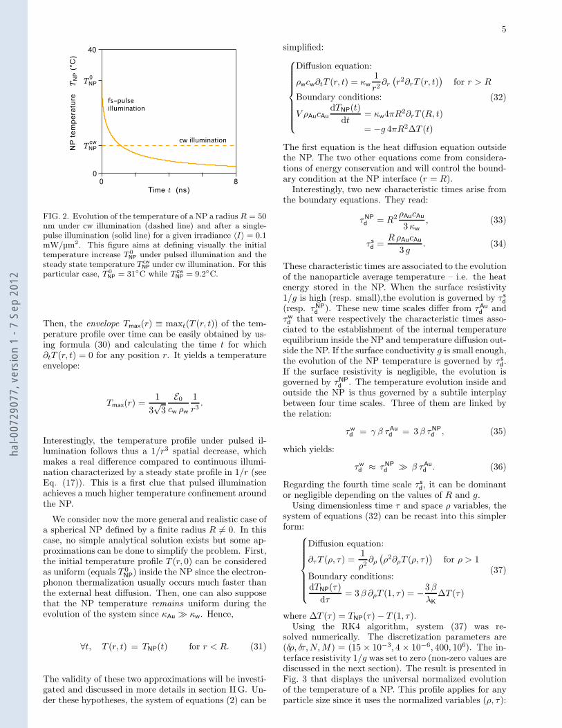
FIG. 2. Evolution of the temperature of a NP a radius R = 50nm under cw illumination (dashed line) and after a single-pulse illumination (solid line) for a given irradiance 〈I〉 = 0.1mW/µm2. This figure aims at defining visually the initialtemperature increase T 0

NP under pulsed illumination and thesteady state temperature T cw

NP under cw illumination. For thisparticular case, T 0

NP = 31◦C while T cwNP = 9.2◦C.

Then, the envelope Tmax(r) ≡ maxt(T (r, t)) of the tem-perature profile over time can be easily obtained by us-ing formula (30) and calculating the time t for which∂tT (r, t) = 0 for any position r. It yields a temperatureenvelope:

Tmax(r) =1

3√3

E0cw ρw

1

r3.

Interestingly, the temperature profile under pulsed il-lumination follows thus a 1/r3 spatial decrease, whichmakes a real difference compared to continuous illumi-nation characterized by a steady state profile in 1/r (seeEq. (17)). This is a first clue that pulsed illuminationachieves a much higher temperature confinement aroundthe NP.

We consider now the more general and realistic case ofa spherical NP defined by a finite radius R 6= 0. In thiscase, no simple analytical solution exists but some ap-proximations can be done to simplify the problem. First,the initial temperature profile T (r, 0) can be consideredas uniform (equals T 0

NP) inside the NP since the electron-phonon thermalization usually occurs much faster thanthe external heat diffusion. Then, one can also supposethat the NP temperature remains uniform during theevolution of the system since κAu ≫ κw. Hence,

∀t, T (r, t) = TNP(t) for r < R. (31)

The validity of these two approximations will be investi-gated and discussed in more details in section IIG. Un-der these hypotheses, the system of equations (2) can be

simplified:

Diffusion equation:

ρwcw∂tT (r, t) = κw1

r2∂r

(

r2∂rT (r, t))

for r > R

Boundary conditions:

V ρAucAudTNP(t)

dt= κw4πR

2∂rT (R, t)

= −g 4πR2∆T (t)

(32)

The first equation is the heat diffusion equation outsidethe NP. The two other equations come from considera-tions of energy conservation and will control the bound-ary condition at the NP interface (r = R).Interestingly, two new characteristic times arise from

the boundary equations. They read:

τNPd = R2 ρAucAu

3 κw, (33)

τ sd =RρAucAu

3 g. (34)

These characteristic times are associated to the evolutionof the nanoparticle average temperature – i.e. the heatenergy stored in the NP. When the surface resistivity1/g is high (resp. small),the evolution is governed by τ sd(resp. τNP

d ). These new time scales differ from τAud andτwd that were respectively the characteristic times asso-ciated to the establishment of the internal temperatureequilibrium inside the NP and temperature diffusion out-side the NP. If the surface conductivity g is small enough,the evolution of the NP temperature is governed by τ sd.If the surface resistivity is negligible, the evolution isgoverned by τNP

d . The temperature evolution inside andoutside the NP is thus governed by a subtile interplaybetween four time scales. Three of them are linked bythe relation:

τwd = γ β τAud = 3 β τNPd , (35)

which yields:

τwd ≈ τNPd ≫ β τAud . (36)

Regarding the fourth time scale τ sd, it can be dominantor negligible depending on the values of R and g.Using dimensionless time τ and space ρ variables, the

system of equations (32) can be recast into this simplerform:

Diffusion equation:

∂τT (ρ, τ) =1

ρ2∂ρ

(

ρ2∂ρT (ρ, τ))

for ρ > 1

Boundary conditions:dTNP(τ)

dτ= 3 β ∂ρT (1, τ) = −3 β

λK∆T (τ)

(37)

where ∆T (τ) = TNP(τ)− T (1, τ).Using the RK4 algorithm, system (37) was re-

solved numerically. The discretization parameters are(δρ, δτ,N,M) = (15 × 10−3, 4 × 10−6, 400, 106). The in-terface resistivity 1/g was set to zero (non-zero values arediscussed in the next section). The result is presented inFig. 3 that displays the universal normalized evolutionof the temperature of a NP. This profile applies for anyparticle size since it uses the normalized variables (ρ, τ):

hal-0

0729

077,

ver

sion

1 -

7 Se

p 20

12

6

0 3210

1

τ = 0.012

τ = 0.04

τ = 0.1

τ = 0.2

τ = 0.4

τ = 1

Normalized coordinate ρ = r/R

No

rma

lize

d T

em

pe

ratu

re

T/T

NP

0

τ = 0

4

τ = 4

1

0110-110-210-310-410-5

TN

P/T

NP0

Normalized time τ

Simulation

Fit

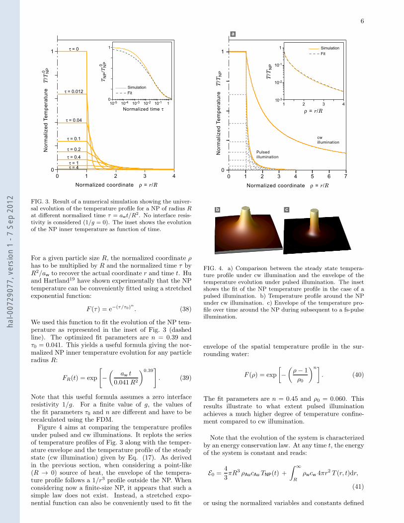
FIG. 3. Result of a numerical simulation showing the univer-sal evolution of the temperature profile for a NP of radius Rat different normalized time τ = awt/R

2. No interface resis-tivity is considered (1/g = 0). The inset shows the evolutionof the NP inner temperature as function of time.

For a given particle size R, the normalized coordinate ρhas to be multiplied by R and the normalized time τ byR2/aw to recover the actual coordinate r and time t. Huand Hartland19 have shown experimentally that the NPtemperature can be conveniently fitted using a stretchedexponential function:

F (τ) = e−(τ/τ0)n

. (38)

We used this function to fit the evolution of the NP tem-perature as represented in the inset of Fig. 3 (dashedline). The optimized fit parameters are n = 0.39 andτ0 = 0.041. This yields a useful formula giving the nor-malized NP inner temperature evolution for any particleradius R:

FR(t) = exp

[

−(

aw t

0.041R2

)0.39]

. (39)

Note that this useful formula assumes a zero interfaceresistivity 1/g. For a finite value of g, the values ofthe fit parameters τ0 and n are different and have to berecalculated using the FDM.Figure 4 aims at comparing the temperature profiles

under pulsed and cw illuminations. It replots the seriesof temperature profiles of Fig. 3 along with the temper-ature envelope and the temperature profile of the steadystate (cw illumination) given by Eq. (17). As derivedin the previous section, when considering a point-like(R → 0) source of heat, the envelope of the tempera-ture profile follows a 1/r3 profile outside the NP. Whenconsidering now a finite-size NP, it appears that such asimple law does not exist. Instead, a stretched expo-nential function can also be conveniently used to fit the

0 721

0

1

Normalized coordinate ρ = r/R

3 4 5 6

Pulsed

illumination

cw

illumination

ρ = r/R

1

10-1

10-2

10-3

1 2 3 4

No

rma

lize

d T

em

pe

ratu

re

T/T

NP

T/T

NP

a

b c

Simulation

Fit

FIG. 4. a) Comparison between the steady state tempera-ture profile under cw illumination and the envelope of thetemperature evolution under pulsed illumination. The insetshows the fit of the NP temperature profile in the case of apulsed illumination. b) Temperature profile around the NPunder cw illumination. c) Envelope of the temperature pro-file over time around the NP during subsequent to a fs-pulseillumination.

envelope of the spatial temperature profile in the sur-rounding water:

F (ρ) = exp

[

−(

ρ− 1

ρ0

)n]

. (40)

The fit parameters are n = 0.45 and ρ0 = 0.060. Thisresults illustrate to what extent pulsed illuminationachieves a much higher degree of temperature confine-ment compared to cw illumination.

Note that the evolution of the system is characterizedby an energy conservation law. At any time t, the energyof the system is constant and reads:

E0 =4

3πR3 ρAucAu TNP(t) +

∫

∞

R

ρwcw 4πr2 T (r, t)dr,

(41)

or using the normalized variables and constants defined

hal-0

0729

077,

ver

sion

1 -

7 Se

p 20

12

7

above, the normalized energy reads:

ǫ0 =TNP(τ)

T 0NP

+

∫

∞

1

3 β ρ2T (ρ, τ)

T 0NP

dρ = 1.

(42)

This conservation law can be conveniently used in nu-merical simulations as a verification of the consistencyof the result. For example, in the simulations shown infigure 3, it varied by less than 0.2%.

F. Finite conductivity of the gold–water interface

In this section, we shall go one step further into therefinement of the analytical description of the problem.We still consider the NP temperature as uniform, but wetake into account a finite interface conductivity g. Theset of equations describing the system is given by (37).

0

1

1 32

Normalized coordinate

ρ = r/R

Normalized time τ

No

rma

lize

d T

em

pe

ratu

re

T/T

NP

0

TN

P(τ

)/T

NP

0

λK=1 λK=0.1

00

1

1 320

λK=0.01

0

1

1 320 0 10

1

b

c

a

τ=0.012τ=0

τ=0.04

τ=0.1

τ=0.2

τ=0.4

τ=1τ=4

τ=0.012

τ=0

τ=0.04

τ=0.1

τ=0.2

τ=0.4τ=1τ=4

τ=0.012

τ=0

τ=0.04

τ=0.1

τ=0.2

τ=0.4τ=1τ=4

Max. watertemperature

Max. w. t.

Max. w. t.

a b

c d

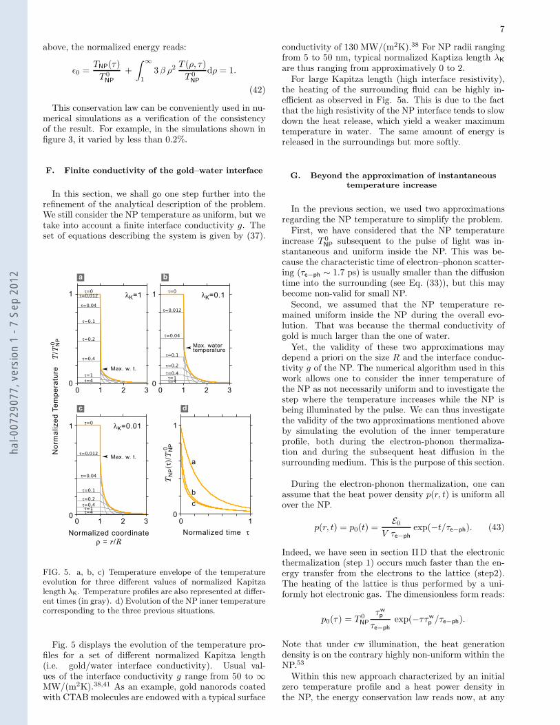
FIG. 5. a, b, c) Temperature envelope of the temperatureevolution for three different values of normalized Kapitzalength λK. Temperature profiles are also represented at differ-ent times (in gray). d) Evolution of the NP inner temperaturecorresponding to the three previous situations.

Fig. 5 displays the evolution of the temperature pro-files for a set of different normalized Kapitza length(i.e. gold/water interface conductivity). Usual val-ues of the interface conductivity g range from 50 to ∞MW/(m2K).38,41 As an example, gold nanorods coatedwith CTAB molecules are endowed with a typical surface

conductivity of 130 MW/(m2K).38 For NP radii rangingfrom 5 to 50 nm, typical normalized Kaptiza length λKare thus ranging from approximatively 0 to 2.For large Kapitza length (high interface resistivity),

the heating of the surrounding fluid can be highly in-efficient as observed in Fig. 5a. This is due to the factthat the high resistivity of the NP interface tends to slowdown the heat release, which yield a weaker maximumtemperature in water. The same amount of energy isreleased in the surroundings but more softly.

G. Beyond the approximation of instantaneous

temperature increase

In the previous section, we used two approximationsregarding the NP temperature to simplify the problem.First, we have considered that the NP temperature

increase T 0NP subsequent to the pulse of light was in-

stantaneous and uniform inside the NP. This was be-cause the characteristic time of electron–phonon scatter-ing (τe−ph ∼ 1.7 ps) is usually smaller than the diffusiontime into the surrounding (see Eq. (33)), but this maybecome non-valid for small NP.Second, we assumed that the NP temperature re-

mained uniform inside the NP during the overall evo-lution. That was because the thermal conductivity ofgold is much larger than the one of water.Yet, the validity of these two approximations may

depend a priori on the size R and the interface conduc-tivity g of the NP. The numerical algorithm used in thiswork allows one to consider the inner temperature ofthe NP as not necessarily uniform and to investigate thestep where the temperature increases while the NP isbeing illuminated by the pulse. We can thus investigatethe validity of the two approximations mentioned aboveby simulating the evolution of the inner temperatureprofile, both during the electron-phonon thermaliza-tion and during the subsequent heat diffusion in thesurrounding medium. This is the purpose of this section.

During the electron-phonon thermalization, one canassume that the heat power density p(r, t) is uniform allover the NP.

p(r, t) = p0(t) =E0

V τe−ph

exp(−t/τe−ph). (43)

Indeed, we have seen in section IID that the electronicthermalization (step 1) occurs much faster than the en-ergy transfer from the electrons to the lattice (step2).The heating of the lattice is thus performed by a uni-formly hot electronic gas. The dimensionless form reads:

p0(τ) = T 0NP

τwpτe−ph

exp(−ττwp /τe−ph).

Note that under cw illumination, the heat generationdensity is on the contrary highly non-uniform within theNP.53

Within this new approach characterized by an initialzero temperature profile and a heat power density inthe NP, the energy conservation law reads now, at any

hal-0

0729

077,

ver

sion

1 -

7 Se

p 20

12

8

1

0

1

0

No

rma

lize

d T

em

pe

ratu

re

T/T

NP0

r (nm) r (nm)

010050 1050

...

No

rma

lize

d T

em

pe

ratu

re

TN

P/T

NP0

1

0

time t (ps)

No

rma

lize

d s

ou

rce

of

he

at

0 6.8

0.48

0.92

0.48

0.92

1

03.2τ

e-ph

exp

(-t/

τ e-p

h)

t = 0

t = 0.14 ps

t = 0.28 ps

t = 3.2 ps

t = 0

t = 0.35 ps

t = 0.70 ps

...

t = 6.8 ps

20

a b

c

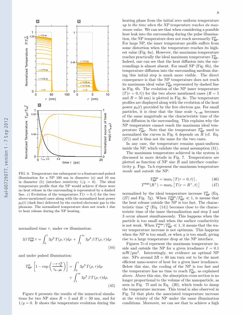
FIG. 6. Temperature rise subsequent to a femtosecond-pulsedillumination for a NP 100 nm in diameter (a) and 10 nmin diameter (b) (interface resistivity 1/g = 0). The idealtemperature profile that the NP would achieve if there wereno heat release in the surrounding is represented by a dashedline. c) Evolution of the temperature T (r = 0, t) for the twoabove-mentioned cases along with the normalized heat powerp0(t) (dark line) delivered by the excited electronic gas to thephonons. The normalized temperature does not reach 1 dueto heat release during the NP heating.

normalized time τ , under cw illumination:

3β T cwNP τ =

∫ 1

0

3ρ2 T (ρ, τ)dρ +

∫

∞

1

3ρ2 β T (ρ, τ)dρ

(44)

and under pulsed illumination:

T 0NP

[

1− exp

(−τ τwdτe−ph

)]

=

∫ 1

0

3ρ2 T (ρ, τ)dρ

+

∫

∞

1

3ρ2 β T (ρ, τ)dρ.

(45)

Figure 6 presents the results of the numerical simula-tions for two NP sizes R = 5 and R = 50 nm, and for1/g = 0. It shows the temperature evolution during the

heating phase from the initial zero uniform temperatureup to the time when the NP temperature reaches its max-

imum value. We can see that when considering a possibleheat leak into the surrounding during the pulse illumina-tion, the NP temperature does not reach necessarily T 0

NP.For large NP, the inner temperature profile suffers fromsome distortion when the temperature reaches its high-est value (Fig. 6a). However, the maximum temperaturereaches practically the ideal maximum temperature T 0

NP.Indeed, one can see that the heat diffusion into the sur-roundings is almost absent. For small NP (Fig. 6b), thetemperature diffusion into the surrounding medium dur-ing this initial step is much more visible. The directconsequence is that the NP temperature does not reachits maximum ideal value T 0

NP represented by dashed linein Fig. 6b. The evolution of the NP inner temperature(T (r = 0, t)) for the two above mentioned cases (R = 5and R = 50 nm) is plotted in Fig. 6c. The temperatureprofiles are displayed along with the evolution of the heatpower p0(t) provided by the free electron gas. For smallparticles, it is clear that the time scale τe−ph becomesof the same magnitude as the characteristic time of theheat diffusion in the surrounding. This explains why theNP temperature cannot reach the maximum ideal tem-perature T 0

NP. Note that the temperature T 0NP used to

normalized the curves in Fig. 6 depends on R (cf. Eq.(27)) and is thus not the same for the two cases.In any case, the temperature remains quasi-uniform

inside the NP, which validate the usual assumption (31).The maximum temperature achieved in the system is

discussed in more details in Fig. 7. Temperatures areplotted as function of NP size R and interface conduc-tivity g. Figs. 7a-b represent the maximum temperatureinside and outside the NP:

TmaxNP = maxt [T (r = 0, t) ] , (46)

Tmax(R+) = maxt[

T (r = R+, t)]

(47)

normalized by the ideal temperature increase T 0NP (Eq.

(27) and Fig. 7g). When TmaxNP /T 0

NP ≪ 1, it means thatthe heat release outside the NP is too fast. The charac-teristic time τwd (Eq. (14)) becomes close to the charac-teristic time of the inner thermalization and step 2 and3 occur almost simultaneously. This happens when theparticle is too small and when the surface conductivityis not weak. When Tmax

w /T 0NP ≪ 1, it means that the wa-

ter temperature increase is not optimum. This happenswhen the NP is too small, or when g is too small, givingrise to a large temperature drop at the NP interface.Figures 7c-d represent the maximum temperature in-

side and outside the NP for a given irradiance I = 0.1mW/µm2. Interestingly, we evidence an optimal NPsize. NPs around 2R = 40 nm turn out to be the mostefficient nano-source of heat for a given laser irradiance.Below this size, the cooling of the NP is too fast andthe temperature has no time to reach T 0

NP, as explainedabove. Above this size, the absorption cross section is nolonger proportional to the volume of the nanoparticle, asseen in Fig. 7f and in Eq. (20), which tends to dampthe temperature increase. This trend is also observed inFig. 7d that plots the associated temperature increaseat the vicinity of the NP under the same illuminationconditions. Moreover, we can see that to achieve a high

hal-0

0729

077,

ver

sion

1 -

7 Se

p 20

12

9

NP

su

rfa

ce

co

nd

uctivity g (x106 W

/mK)

NP radius R (nm)

0

1

0

46°C

150

200

250

300

400

500

700

1000

1500

∞

100

50

150

200

250

300

400

500

700

1000

1500

∞

100

50

σabs

10

5 10 15 20 30 40 50 5 10 15 20 30 40 505 10 15 20 30 40 50 5 10 15 20 30 40 50

TNP /TNP0max TNP

max

NP radius R (nm)

NP radius R (nm)

40

0

(x103 nm2)

0 50

10

0

60

00 500 50

TNP0

NP radius R (nm)

Tcw(R+)

(°C)

(°C)

~R3

~R2

T

(R+)/TNP0max T (R+)

max

η = T (R+)/T

cw(R+)

max

150

200

250

300

400

500

700

1000

1500

∞

100

50

5 10 15 20 30 40 50

1

10

102

0.781.11.62.94.48.325

1.31.72.64.87.51442

1.62.23.46.3101956

1.82.64.07.5122366

2.02.84.58.5132676

2.13.04.88.5132675

2.33.35.411173296

2.43.55.9121936106

2.63.96.4132141120

2.84.26.9142345134

2.94.47.4152549148

3.24.98.6183061184103

a b c d

e

f g h

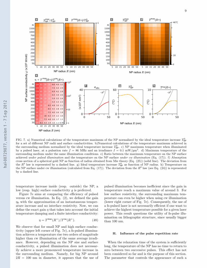
FIG. 7. a) Numerical calculations of the temperature maximum of the NP normalized by the ideal temperature increase T 0

NP

for a set of different NP radii and surface conductivities. b)Numerical calculations of the temperature maximum achieved inthe surrounding medium normalized by the ideal temperature increase T 0

NP. c) NP maximum temperature when illuminatedby a pulsed laser, at a pulsation rate f = 86 MHz and an irradiance I = 0.1 mW/µm2. d) Maximum temperature of thesurrounding medium under the same illumination conditions. e) Ratio between the maximum temperature on the NP surfaceachieved under pulsed illumination and the temperature on the NP surface under cw illumination (Eq. (17)). f) Absorptioncross section of a spherical gold NP as function of radius obtained from Mie theory (Eq. (25)) (solid line). The deviation fromthe R3 law is represented by a dashed line. g) Ideal temperature increase T 0

NP as function of NP radius. h) Temperature onthe NP surface under cw illumination (calculated from Eq. (17)). The deviation from the R2 law (see Eq. (24)) is representedby a dashed line.

temperature increase inside (resp. outside) the NP, alow (resp. high) surface conductivity g is preferred.Figure 7e aims at comparing the efficiency of pulsed

versus cw illumination. In Eq. (2), we defined the gainη0 with the approximation of an instantaneous temper-ature increase and no interface resistivity. Now, we candefine the exact gain η that takes into account the initialtemperature damping and a finite interface conductivity:

η = Tmax(R+)/T cw(R+). (48)

We observe that for small NP and high surface conduc-tivity (upper left corner of Fig. 7e), a fs-pulsed illumina-tion achieves a temperature rise two orders of magnitudehigher than cw illumination of the same average irradi-ance. However, depending on the NP size and surfaceconductivity, a pulsed illumination does not necessar-ily achieve a more pronounced temperature increase inthe surrounding medium. Namely, for big NP around2R = 100 nm in diameter, it appears that the use of

pulsed illumination becomes inefficient since the gain intemperature reach a maximum value of around 3. Forlow surface resistivity, the surrounding maximum tem-perature can even be higher when using cw illumination(lower right corner of Fig. 7e). Consequently, the use ofa fs-pulsed laser is not necessarily efficient if one want toachieve the highest temperature possible for a given laserpower. This result questions the utility of fs-pulse illu-mination on lithographic structure, since usually biggerthan 100 nm.

H. Influence of the pulse repetition rate

When the relaxation time of the system is sufficientlylong, the temperature of the NP has no time to return tozero between two successive pulses. This effect has notbeen considered so far and is the purpose of this section.The parameter that controls the appearance of such a

hal-0

0729

077,

ver

sion

1 -

7 Se

p 20

12

10

Time t (ns)

NP

te

mp

era

ture

T

NP (

°C)

0 10020

0 100200

8

0

20

TNP

cw

ξ=0.036 / R=10 nm

ξ=0.89 / R=50 nm

a

b

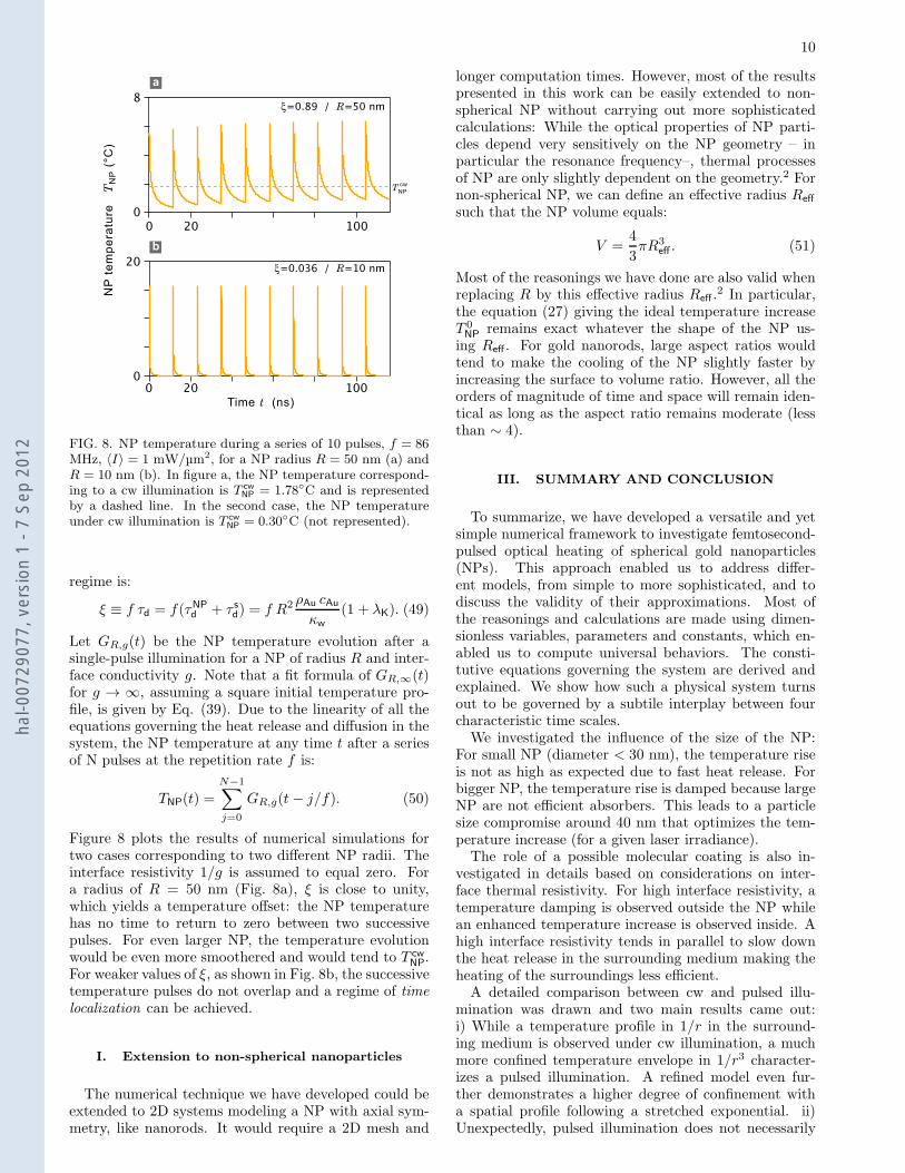
FIG. 8. NP temperature during a series of 10 pulses, f = 86MHz, 〈I〉 = 1 mW/µm2, for a NP radius R = 50 nm (a) andR = 10 nm (b). In figure a, the NP temperature correspond-ing to a cw illumination is T cw

NP = 1.78◦C and is representedby a dashed line. In the second case, the NP temperatureunder cw illumination is T cw

NP = 0.30◦C (not represented).

regime is:

ξ ≡ f τd = f(τNPd + τ sd) = f R2 ρAu cAu

κw(1 + λK). (49)

Let GR,g(t) be the NP temperature evolution after asingle-pulse illumination for a NP of radius R and inter-face conductivity g. Note that a fit formula of GR,∞(t)for g → ∞, assuming a square initial temperature pro-file, is given by Eq. (39). Due to the linearity of all theequations governing the heat release and diffusion in thesystem, the NP temperature at any time t after a seriesof N pulses at the repetition rate f is:

TNP(t) =N−1∑

j=0

GR,g(t− j/f). (50)

Figure 8 plots the results of numerical simulations fortwo cases corresponding to two different NP radii. Theinterface resistivity 1/g is assumed to equal zero. Fora radius of R = 50 nm (Fig. 8a), ξ is close to unity,which yields a temperature offset: the NP temperaturehas no time to return to zero between two successivepulses. For even larger NP, the temperature evolutionwould be even more smoothered and would tend to T cw

NP.For weaker values of ξ, as shown in Fig. 8b, the successivetemperature pulses do not overlap and a regime of time

localization can be achieved.

I. Extension to non-spherical nanoparticles

The numerical technique we have developed could beextended to 2D systems modeling a NP with axial sym-metry, like nanorods. It would require a 2D mesh and

longer computation times. However, most of the resultspresented in this work can be easily extended to non-spherical NP without carrying out more sophisticatedcalculations: While the optical properties of NP parti-cles depend very sensitively on the NP geometry – inparticular the resonance frequency–, thermal processesof NP are only slightly dependent on the geometry.2 Fornon-spherical NP, we can define an effective radius Reff

such that the NP volume equals:

V =4

3πR3

eff . (51)

Most of the reasonings we have done are also valid whenreplacing R by this effective radius Reff .

2 In particular,the equation (27) giving the ideal temperature increaseT 0NP remains exact whatever the shape of the NP us-

ing Reff . For gold nanorods, large aspect ratios wouldtend to make the cooling of the NP slightly faster byincreasing the surface to volume ratio. However, all theorders of magnitude of time and space will remain iden-tical as long as the aspect ratio remains moderate (lessthan ∼ 4).

III. SUMMARY AND CONCLUSION

To summarize, we have developed a versatile and yetsimple numerical framework to investigate femtosecond-pulsed optical heating of spherical gold nanoparticles(NPs). This approach enabled us to address differ-ent models, from simple to more sophisticated, and todiscuss the validity of their approximations. Most ofthe reasonings and calculations are made using dimen-sionless variables, parameters and constants, which en-abled us to compute universal behaviors. The consti-tutive equations governing the system are derived andexplained. We show how such a physical system turnsout to be governed by a subtile interplay between fourcharacteristic time scales.We investigated the influence of the size of the NP:

For small NP (diameter < 30 nm), the temperature riseis not as high as expected due to fast heat release. Forbigger NP, the temperature rise is damped because largeNP are not efficient absorbers. This leads to a particlesize compromise around 40 nm that optimizes the tem-perature increase (for a given laser irradiance).The role of a possible molecular coating is also in-

vestigated in details based on considerations on inter-face thermal resistivity. For high interface resistivity, atemperature damping is observed outside the NP whilean enhanced temperature increase is observed inside. Ahigh interface resistivity tends in parallel to slow downthe heat release in the surrounding medium making theheating of the surroundings less efficient.A detailed comparison between cw and pulsed illu-

mination was drawn and two main results came out:i) While a temperature profile in 1/r in the surround-ing medium is observed under cw illumination, a muchmore confined temperature envelope in 1/r3 character-izes a pulsed illumination. A refined model even fur-ther demonstrates a higher degree of confinement witha spatial profile following a stretched exponential. ii)Unexpectedly, pulsed illumination does not necessarily

hal-0

0729

077,

ver

sion

1 -

7 Se

p 20

12

11

achieve much higher temperature increase in the sur-roundings compared to cw, especially for nanoparticlesbigger than 100 nm (typically lithographic plasmonicstructures). It can even be worse when the gold parti-cle is endowed with a poor thermal surface conductivity(due to an hydrophobic molecular coating for example).Finally, the influence of the repetition rate is discussed

and two regimes are identified depending on the NP ra-dius R and the pulsation rate f : One time-localizationregime, where the temperature increase is confined spa-tially and temporally and one regime that tends to re-semble to the regime observed under cw illumination.Within this work, we restricted ourselves to gold

nanoparticles with spherical geometry (radius R), butmost of the results obtained herein are also valid for non-

spherical particles when considered as particles of char-acteristic size R. The numerical techniques we developedcould also be refined to address problems with 2D sym-metries requiring a longer computation time. This ver-satile numerical technique could also take into accountother materials than gold and water and various pulsedurations, from femto- to nanosecond-scales.

ACKNOWLEDGMENTS

We thank Christian Girard, Philippe Refregier,Damien Riedel and Jerome Wenger for helpful discus-sions.

∗ guillaume.baffou@fresnel.fr1 A. O. Govorov and H. H. Richardson, Nano Today 2, 30(2007).

2 G. Baffou, R. Quidant, and F. J. Garcıa de Abajo, ACSnano 4, 709 (2010).

3 A. Nitzan and L. E. Brus, J. Chem. Phys. 75, 2205 (1981).4 W. A. Challener, C. Peng, A. V. Itagi, D. Karns, W. Peng,Y. Peng, X. M. Yang, X. Zhu, N. J. Gokemeijer, Y.-T.Hsia, G. Ju, R. E. Rottmayer, M. A. Seigler, and E. C.Gage, Nat. Photon. 3, 220 (2009).

5 L. Cao, D. Barsic, A. Guichard, and M. Brongersma, NanoLett. 7, 3523 (2007).

6 D. Pissuwan, S. M. Valenzuela, and M. B. Cortie, TrendsBiotechnol. 24, 62 (2006).

7 P. K. Jain, I. H. El-Sayed, and M. A. El-Sayed, NanoToday 2, 18 (2007).

8 S. Lal, S. E. Clare, and N. J. Halas, Acc. Chem. Res. 41,1842 (2009).

9 G. Han, P. Ghosh, M. De, and V. M. Rotello,NanoBioTechnology 3, 40 (2007).

10 A. G. Skirtach, C. Dejugnat, D. Braun, A. S. Susha, A. L.Rogach, W. J. Parak, H. Mohwald, and G. B. Sukhorukov,Nano Lett. 5, 1371 (2005).

11 L. Tong, Q. Wei, A. Wei, and J. X. Cheng, Photochemistryand photobiology 85, 21 (2009).

12 J. Butet, J. Duboisset, G. Bachelier, I. Russier-Antoine,E. Benichou, C. Jonin, and P. F. Brevet, Nano Lett. 10,1717 (2010).

13 W. Lu, Q. Huang, G. Ku, X. Wen, M. Zhou, D. Guzatov,P. Brecht, R. Su, A. Oraevsky, L. V. Wang, and C. Li,Biomaterials 31, 2617 (2010).

14 S. Mallidi, T. Larson, J. Aaron, K. Sokolov, andS. Emelianov, Opt. Express 15, 6583 (2007).

15 A. Vogel and V. Venugopalan, Chem. Rev. 103, 577(2003).

16 R. R. Anderson and J. A. Parrish, Science 220, 524 (1983).17 V. K. Pustovalov, Chem. Phys. 308, 103 (2005).18 A. N. Volkov, C. Sevilla, and L. V. Zhigilei, Appl. Surf.

Sci. 253, 6394 (2007).19 M. Hu and G. V. Hartland, J. Phys. Chem. B 106, 7029

(2002).20 M. Hu, X. Wang, G. V. Hartland, P. Mulvaney, J. P. Juste,

and J. E. Sader, J. Am. Chem. Soc. 125, 14925 (2003).21 A. L. Tchebotareva, P. V. Ruijgrok, and M. Orrit, Laser

Photonics Rev. 4, 581 (2010).22 N. Large, L. Saviot, J. Margueritat, J. Gonzalo, C. N.

Afonso, A. Arbouet, P. Langot, A. Mlayah, and J. Aizpu-rua, Nano Lett. 9, 3732 (2009).

23 P. Chakravarty, W. Qian, M. A. El-Sayed, and M. R.Prausnitz, Nature Nanotech. 5, 607 (2010).

24 A. Vogel, J. Noack, G. Huttman, and G. Paltauf, Appl.Phys. B 81, 1015 (2005).

25 D. Lapotko, Opt. Express 17, 2538 (2009).26 E. Lukianova-Hleb, L. Hu, Y. andLatterini, L. Tarpani,

S. Lee, R. A. Drezek, J. H. Hafner, and D. O. Lapotko,ACS nano 4, 2109 (2010).

27 A. Vogel, N. Linz, S. Freidank, and G. Paltauf, Phys. Rev.Lett. 100, 038102 (2008).

28 V. Kotaidis, C. Dahmen, G. von Plessen, F. Springer, andA. Plech, J. Chem. Phys. 124, 184702 (2006).

29 S. Link, C. Burda, B. Nikoobakht, and M. A. El-Sayed, J.Phys. Chem. B 104, 6152 (2000).

30 E. Lukianova-Hleb, L. J. E. Anderson, S. Lee, J. H.Hafner, and D. O. Lapotko, Phys. Chem. Chem. Phys.12, 12237 (2010).

31 A. Plech, V. Kotaidis, S. Gresillon, C. Dahmen, andG. von Plessen, Phys. Rev. B 70, 195423 (2004).

32 E. Sassaroli, K. C. P. Li, and B. E. O’Neill, Phys. Med.Biol. 54, 5541 (2009).

33 E. Y. Hleb and D. O. Lapotko, Nanotechology 19, 355702(2008).

34 O. Ekici, R. K. Harrison, N. J. Durr, D. S. Eversole,M. Lee, and A. Ben-Yakar, J. Phys. D: Appl. Phys. 41,185501 (2008).

35 M. Hu, H. Petrova, and G. V. Hartland, Chem. Phys. Lett.391, 220 (2004).

36 S. Merabia, P. Keblinski, L. Joly, L. J. Lewis, and J. L.Barrat, Phys. Rev. E 79, 021404 (2009).

37 S. Merabia, S. Shenogin, L. Joly, P. Keblinski, and J. L.Barrat, PNAS 106, 15113 (2009).

38 A. J. Schmidt, J. D. Alper, M. Chiesa, G. Chen, S. K. Das,and K. Hamad-Schifferli, J. Phys. Chem. C 112, 13320(2008).

39 O. M. Wilson, X. Hu, D. G. Cahill, and P. V. Braun, Phys.Rev. B 66, 224301 (2002).

40 Z. Ge, D. G. Cahill, and P. V. Braun, J. Phys. Chem. B108, 18870 (2010).

41 J. Alper and K. Hamad-Schifferli, Langmuir 26, 3786(2010).

42 Handbook of Physics (Springer, 2000).43 J. C. Butcher, Numerical methods for ordinary differential

equations (John Wiley & Sons, 2003).44 G. Baffou, R. Quidant, and C. Girard, Phys. Rev. B 82,

165424 (2010).45 P. K. Jain, K. S. Lee, I. H. El-Sayed, and M. A. El-Sayed,

J. Phys. Chem. B 110, 7238 (2006), ISSN 1520-6106.

hal-0

0729

077,

ver

sion

1 -

7 Se

p 20

12

12

46 C. F. Bohren and D. R. Huffman, Absorption and scatter-

ing of light by small particles (Wiley interscience, 1983).47 P. Grua, J. P. Morreeuw, H. Bercegol, G. Jonusauskas,

and F. Vallee, Phys. Rev. B 68, 035424 (2003).48 H. Inouye, K. Tanaka, I. Tanahashi, and K. Hirao, Phys.

Rev. B 57, 11334 (1998).49 A. Arbouet, C. Voisin, D. Christofilos, P. Langot,

N. Del Fatti, F. Vallee, J. Lerme, G. Celep, E. Cot-tancin, M. Gaudry, M. Pellarin, M. Broyer, M. Maillard,M. P. Pileni, and M. Treguer, Phys. Rev. Lett. 90, 177401(2003).

50 W. Huang, W. Qian, M. A. El-Sayed, Y. Ding, and Z. L.Wang, J. Phys. Chem. C 111, 10751 (2007).

51 J. H. Hodak, A. Henglein, and G. V. Hartland, J. Chem.Phys. 111, 8613 (1999).

52 S. Link, C. Burda, Z. L. Wang, and M. A. El-Sayed, J.Chem. Phys. 111, 1255 (1999).

53 G. Baffou, R. Quidant, and C. Girard, Appl. Phys. Lett.94, 153109 (2009).

Appendix A: Numerical algorithm

In this section, we explain and detail how the physi-cal system was modeled using a finite difference method(FDM) and in particular what the RK4 algorithm con-sists in.

We shall specifically use in this section the equationsand the formalism based on dimensionless space andtime variables (ρ and τ) and dimensionless constants andparameters (β, γ and λK).

1. Model assuming a uniform NP temperature

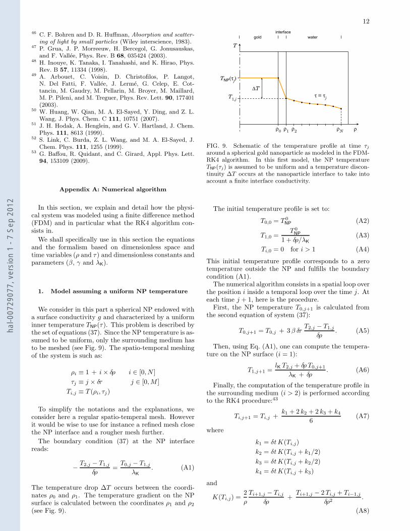
We consider in this part a spherical NP endowed witha surface conductivity g and characterized by a uniforminner temperature TNP(τ). This problem is described bythe set of equations (37). Since the NP temperature is as-sumed to be uniform, only the surrounding medium hasto be meshed (see Fig. 9). The spatio-temporal meshingof the system is such as:

ρi ≡ 1 + i× δρ i ∈ [0, N ]

τj ≡ j × δτ j ∈ [0,M ]

Ti,j ≡ T (ρi, τj)

To simplify the notations and the explanations, weconsider here a regular spatio-temperal mesh. Howeverit would be wise to use for instance a refined mesh closethe NP interface and a rougher mesh further.

The boundary condition (37) at the NP interfacereads:

− T2,j − T1,jδρ

=T0,j − T1,j

λK. (A1)

The temperature drop ∆T occurs between the coordi-nates ρ0 and ρ1. The temperature gradient on the NPsurface is calculated between the coordinates ρ1 and ρ2(see Fig. 9).

τ = τj

ρ0

T

ρ

gold water

ρ1

ρN

interface

T1,j

TNP(τj)

ρ2

∆T

FIG. 9. Schematic of the temperature profile at time τjaround a spherical gold nanoparticle as modeled in the FDM-RK4 algorithm. In this first model, the NP temperatureTNP(τj) is assumed to be uniform and a temperature discon-tinuity ∆T occurs at the nanoparticle interface to take intoaccount a finite interface conductivity.

The initial temperature profile is set to:

T0,0 = T 0NP (A2)

T1,0 =T 0NP

1 + δρ/λK(A3)

Ti,0 = 0 for i > 1 (A4)

This initial temperature profile corresponds to a zerotemperature outside the NP and fulfills the boundarycondition (A1).The numerical algorithm consists in a spatial loop over

the position i inside a temporal loop over the time j. Ateach time j + 1, here is the procedure.First, the NP temperature T0,j+1 is calculated from

the second equation of system (37):

T0,j+1 = T0,j + 3 β δτT2,j − T1,j

δρ. (A5)

Then, using Eq. (A1), one can compute the tempera-ture on the NP surface (i = 1):

T1,j+1 =lK T2,j + δρ T0,j+1

λK + δρ. (A6)

Finally, the computation of the temperature profile inthe surrounding medium (i > 2) is performed accordingto the RK4 procedure:43

Ti,j+1 = Ti,j +k1 + 2 k2 + 2 k3 + k4

6(A7)

where

k1 = δtK(Ti,j)

k2 = δtK(Ti,j + k1/2)

k3 = δtK(Ti,j + k2/2)

k4 = δtK(Ti,j + k3)

and

K(Ti,j) =2

ρ

Ti+1,j − Ti,jδρ

+Ti+1,j − 2Ti,j + Ti−1,j

δρ2.

(A8)

hal-0

0729

077,

ver

sion

1 -

7 Se

p 20

12

13

Ti,j

τ = τj

ρN1

ρ1

T

ρ

gold water

ρ2

ρN1+N2

interface

ρi

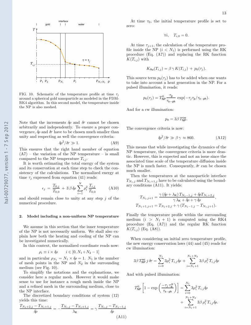
FIG. 10. Schematic of the temperature profile at time τjaround a spherical gold nanoparticle as modeled in the FDM-RK4 algorithm. In this second model, the temperature insidethe NP is also meshed.

Note that the increments δρ and δτ cannot be chosenarbitrarily and independently. To ensure a proper con-vergence, δρ and δτ have to be chosen much smaller thanunity and respecting as well the convergence criteria:

δρ2/δτ ≫ 1. (A9)

This ensures that the right hand member of equation(A7) – the variation of the NP temperature – is smallcompared to the NP temperature Ti,j.It is worth estimating the total energy of the system

and its conservation at each time step to check the con-sistency of the calculations. The normalized energy attime τj expressed from equation (41) reads:

ǫj =T0,jT0,0

+ 3 β δρN∑

i=1

ρ2iTi,jT0,0

(A10)

and should remain close to unity at any step j of thenumerical procedure.

2. Model including a non-uniform NP temperature

We assume in this section that the inner temperatureof the NP is not necessarily uniform. We shall also ex-plain how both the heating and cooling of the NP canbe investigated numerically.In this context, the normalized coordinate reads now:

ρi ≡ i× δρ i ∈ [0, N1+N2 − 1]

and in particular ρN1= N1 × δρ = 1. N1 is the number

of mesh points in the NP and N2 in the surroundingmedium (see Fig. 10).To simplify the notations and the explanations, we

consider here a regular mesh. However it would makesense to use for instance a rough mesh inside the NPand a refined mesh in the surrounding medium, close tothe NP interface.The discretized boundary conditions of system (12)

yields this time:

TN1+2,j − TN1+1,j

δρ= −TN1,j − TN1+1,j

λK= γ

TN1,j − TN1−1,j

δρ

(A11)

At time τ0, the initial temperature profile is set tozero:

∀i, Ti,0 = 0.

At time τj+1, the calculation of the temperature pro-file inside the NP (i < N1) is performed using the RKprocedure (Eq. (A7)) and replacing the RK functionK(Ti,j) with

KAu(Ti,j) = β γ K(Ti,j) + p0(τj).

This source term p0(τj) has to be added when one wantsto take into account a heat generation in the NP. For apulsed illumination, it reads:

p0(τj) = T 0NP

τpτe−ph

exp(−τjτp/τe−ph).

And for a cw illumination:

p0 = 3β T cwNP.

The convergence criteria is now:

δρ2/δτ ≫ β γ ≈ 860. (A12)

This means that while investigating the dynamics of theNP temperature, the convergence criteria is more dras-tic. However, this is expected and not an issue since theassociated time scale of the temperature diffusion insidethe NP is much faster. Consequently, δτ can be chosenmuch smaller.

Then the temperatures at the nanoparticle interfaceTN1,j and TN1+1,j have to be calculated using the bound-ary conditions (A11). It yields:

TN1,j+1 =γ (δρ+ λK)TN1−1,j + δρTN1+2,j

γ λK + δρ+ γ δρ,

TN1+1,j+1 = TN1+2,j + γ (TN1−1,j − TN1,j+1).

Finally the temperature profile within the surroundingmedium (i > N1 + 1) is computed using the RK4procedure (Eq. (A7)) and the regular RK functionK(Ti,j) (Eq. (A8)).

When considering an initial zero temperature profile,the new energy conservation laws (44) and (45) reads forcw illumination:

3β TwcNP j δτ =

N1∑

i=0

3ρ2i Ti,jδρ +

N1+N2∑

i=N1+1

3β ρ2i Ti,jδρ

And with pulsed illumination:

T 0NP

[

1− exp

(−τj τwdτe−ph

)]

=

N1∑

i=0

3ρ2i Ti,jδρ

+

N1+N2∑

i=N1+1

3β ρ2i Ti,jδρ.

hal-0

0729

077,

ver

sion

1 -

7 Se

p 20

12