Generalized Velocity Obstacles

David Wilkie Jur van den Berg Dinesh Manocha

Abstract— We address the problem of real-time navigationin dynamic environments for car-like robots. We present anapproach to identify controls that will lead to a collisionwith a moving obstacle at some point in the future. Ourapproach generalizes the concept of velocity obstacles, whichhave been used for navigation among dynamic obstacles, andtakes into account the constraints of a car-like robot. We usethis formulation to find controls that will allow collision freenavigation in dynamic environments. Finally, we demonstratethe performance of our algorithm on a simulated car-like robotamong moving obstacles.

I. INTRODUCTION

The problem of computing a collision-free path for arobot moving among dynamic obstacles is important in manyrobotics applications, including automated transportation sys-tems, automated factories, and applications involving robot-human interactions, such as robotic wheelchairs [18]. Inmany of these applications, the robot of interest is a car-likerobot and subject to non-holonomic kinematic constraints.

In this paper, we extend the velocity obstacle conceptto handle such robots. This concept was introduced byFiorini and Shiller [2] for navigating robots among arbitrarilymoving obstacles and has been extended to multi-agentnavigation and real-world applications. The velocity obstacleformulation works well for robots that can move in anyspecified direction, but it may not capture the movement ofcar-like robots well, which can only move, at any instant,with a velocity parallel to the rear wheels.

In this paper, we present an extension of the velocityobstacle concept to handle robots with kinematic constraints.We present a new algebraic formulation of the velocityobstacle in terms of the set of controls that can, at some pointin the future, result in a collision. This generalized velocityobstacle approach is used to safely navigate a car-like robotamong dynamic obstacles.

Our approach focuses on iteratively sensing and avoidingobstacles. The intended use is within sense-plan-act iter-ations that could be incorporated in a global planner ora partial motion planner, a concept introduced in [16] tocompute global collision-free paths incrementally.

The rest of this paper is organized as follows. SectionII discusses the related work and focuses on techniques for

Department of Computer Science, College of Arts and Sciences, Univer-sity of North Carolina, 201 South Columbia Street, Chapel Hill, NC 27599,USA. E-mail: {wilkie, berg, dm}@cs.unc.edu

For further project details, code, and videos, refer tohttp://gamma.cs.unc.edu/NHRVO.

This work was supported in part by ARO contracts DAAD19-02-1-0390and W911NF-04-1-0088, NSF awards 0400134, 0429583, and 0404088,DARPA/RDECOM contract N61339-04-C-0043, Intel, and the UNC MeritAssistantship.

navigating car-like robots. Section III provides backgroundinformation on velocity obstacles and the issues in usingthem for car-like robots. Section IV introduces the ideaof generalized velocity obstacles. In Section V, we applygeneralized velocity obstacles to a car-like robot movingamong dynamic obstacles, and highlight the algorithm’sperformance. Section VI presents concluding remarks onfuture work and some deficiencies of the approach.

II. PRIOR WORK

In this section, we give a brief overview of related workon navigating agents and robots in dynamic environments.

Numerous motion planning algorithms have been devel-oped for car-like robots in static environments. In [11], thenotion of a car-like robot was formalized, and the fact that apath for a holonomic robot lying fully in open regions of theconfiguration space can always be transformed into a feasiblepath for a nonholonomic robot was proven. Laumond et al.[11] also provided an algorithm to generate a feasible pathfor a nonholonomic robot from a path found for a holonomicrobot. Smooth planning for car-like robots among obstacleswas first proposed by Scheuer et al. [20], and this ideawas extended by Lamiraux and Laumond [9], which uses asteering function rather than computing clothoid curves.

Approaches applicable to car-like robots have been de-veloped for complete trajectory planning among movingobstacles, such as [4], [6], [26]. Some of these approachesdecompose the problem of planning in a dynamic environ-ment into generating a feasible path and planning a velocityprofile to safely traverse the path, [7], [15], [25].

An alternative to complete planning is to plan for therobot as it acts, taking new sensor inputs as they arrive andplanning locally. Some of the prominent work in this areais based on velocity obstacles (VO) [1], [2]. The idea is todefine a set of velocities that would, if used as a control forthe agent, lead to a collision with an obstacle at some timein the future. In its original formulation, VO was applied toagents moving along piecewise linear velocities and assumedthe obstacles would be moving at constant velocities over atime interval. The idea was extended in [21], which used theidea of a non-linear velocity obstacle to define a VO for anobstacle moving along an arbitrary trajectory, which needs tobe known in advance. Large et al. [10] addressed the problemof predicting the motion of obstacles and applied the resultto a car-like robot, but they still model the agent velocityas a piecewise linear function. An extension of VO by vanden Berg et al., the Reciprocal Velocity Obstacle, appearedin [24], which addressed the oscillation issue that occurs inthe VO formulation. This work was expanded to address the

Fig. 1. The velocity obstacle V OA|B for robot A relative to dynamicobstacle B. The cone of velocities that would lead to a collision in thestatic case is translated by vB. Note that as the velocity vA is inside thevelocity obstacle, the relative velocity, vA − vB, leads to a collision.

n-body collision avoidance problem [23]. The VO concepthas been applied to control real robots, such as in [17], [18].

An analytical approach to compute a trajectory for anon-holonomic robot moving among dynamic obstacles isgiven in [19], and this approach was combined with rapidly-exploring random trees (RRTs) in [13]. Another approach tonavigating non-holonomic agents in dynamic environmentsis presented in [14].

Some iterative approaches to planning in dynamic envi-ronments exist, such as [3], [6], [10], that seek to balancethis local planning strategy with reaching a goal.

Finally, another approach to navigation among dynamicobstacles is to create potential fields for obstacles [8], [22].

III. VELOCITY OBSTACLES

In this section, we review the concept of velocity obstaclesand discuss its application to car-like robots.

A. Definition

For a disc-shaped agent A and a disc-shaped movingobstacle B with radii rA and rB , respectively, the velocityobstacle for A induced by B, denoted V OA|B , is the set ofvelocities for A that would, at some point in the future, resultin a collision with B. This set is defined geometrically. First,let pA and pB be the center points of A and B, respectively,and let B be a disc centered at pB with a radius equal to thesum of A’s and B’s. This is generalized as the Minkowskisum. If B is static (i.e. not moving), we could define a cone,C, of velocities for A that would lead to a collision with B as

the set of rays shot from pA that intersect the boundary of B.To derive a velocity obstacle from this, we simply translatethe cone C by the velocity vB of B, as shown in Figure 1.More formally:

V OA|B = {v | ∃t > 0 :: pA + t(v − vB) ∈ B}. (1)

B. Robots with Kinematic Constraints

For many kinematically constrained robots, such as car-like robots, the set of feasible velocities at any instant isa single velocity – the specific velocity in the direction ofthe rear wheels. One way to workaround this constraint anduse velocity obstacles is to use the set of velocities thatcan be achieved over some time interval τ [2]. However,this approach does not guarantee collision-free navigation:consider the set of velocities, V , that a car-like robot canreach after τ seconds. VOs can be constructed for the robot,and a velocity from V outside the VOs can be selected tonavigate the robot. In this case, a car-like robot will actuallyneed to follow an arc to achieve the selected velocity, andthe VOs provide no guarantee that this arc will be collision-free. Additionally, the robot will be at a different positionwhen it achieves the selected velocity, but the VOs thatwere computed using the robot’s initial position, and thusthe velocity is no longer guaranteed to be collision-free. Toalleviate these issues, we can select a small value for τ , butthis has some implications for navigation: as τ decreases,the set of velocities that are being considered by the robotbecomes smaller, and the robot can miss feasible controls.

IV. GENERALIZED VELOCITY OBSTACLES

In this section, we define a new concept called the Gen-eralized Velocity Obstacle. This is a generalization of thevelocity obstacle concept and seeks to address the difficultyof using velocity obstacles with kinematically constrainedagents (e.g. car-like robots).

A. Definition

The generalized obstacle can be defined as follows. Givenan obstacle B, let us denote its position at time t by B(t).Similarly, given the position of agent A at time t = 0 anda control u, let us denote the position agent A will haveafter undertaking u for time interval t by A(t, u). Here,a control u is a set of inputs to the kinodynamic modelthat results in a change in the robot’s configuration. If wecontinue to restrict our attention to agents and obstaclesthat are circularly shaped, we can define the obstacle in thecontrol space as

{u | ∃t > 0 :: ‖A(t, u)−B(t)‖ < rA + rB}. (2)

Given a specific set of kinematic constraints for somesystem, we can apply the V OA|B formulation as follows.Let tmin(u) be the time at which the distance between thecenters of A and B is minimal for a given control u for A:

tmin(u) = arg mint>0

‖A(t, u)−B(t)‖. (3)

Fig. 2. The kinematic model of a simple car.

If a closed expression for tmin(u) is obtained, for example bysolving ∂‖A(t,u)−B(t)‖

∂t = 0 for t, then it may also be possiblethat an explicit equation for the velocity obstacle can befound by solving ‖A(tmin(u), u)−B(tmin(u))‖ < rA + rBfor u.

For the cases when a closed form solution is not obtain-able, this approach can be used in a sampling scheme. Inthis case, controls in U are sampled. For each control u,the minimum distance that agent A and obstacle B wouldachieve were A to use control u is numerically calculated.This distance determines whether the control would becollision free.

B. Example: an Unconstrained Robot

To illustrate this approach, let us take as an example anagent without kinematic constraints – the type of agent forwhich the original velocity obstacle formulation was definedby Fiorini and Shiller [1]. In this case, a control u for Adirectly corresponds to a velocity v for A. Let us assume,without loss of generality, that the initial position of A is atthe origin. Let an obstacle B be at the initial position pBand be moving with the velocity vB . Then we have

A(t,v) = tv, (4)B(t) = pB + tvB . (5)

Solving for t the equation ∂‖A(t,u)−B(t)‖∂t = 0 gives the

equation for tmin(v):

tmin(v) =pB · (v − vB)‖v − vB‖2

. (6)

Reducing ‖A(tmin(v),v) − B(tmin(v))‖ < rA + rB yieldsan expression that is true for all velocities in the velocityobstacle.

This velocity obstacle is identical to those derived in [2]and can be used for navigation in a fast sampling algorithm.A preferred control u∗ can be computed based on a functionof the current configuration and the goal configuration, andthe control closest to the preferred control but outside allvelocity obstacles can be used to navigate the robot. Thedifference between the two definitions of VOs in (1) and (2)is that we can generalize the latter to incorporate kinematicconstraints, as shown in Section V.

Fig. 3. The agent, green, navigates among numerous obstacles, in red,while heading toward a goal in the upper right corner.

Fig. 4. Obstacle B is moving along trajectory B(t), and agent A istrying to evade. A tests control u′, which generates trajectory A(t, u′).The minimum distance between B and A occurs at tmin, and this distanceis greater than the sum of the radii. Therefore, control u′ is not in thevelocity obstacle.

C. Finite Time Horizon

In practice it is useful to limit the velocity obstacle toaddress only those collisions that will happen before a timehorizon, tlim. Beyond the time horizon the collisions areassumed to be too unlikely to consider. For the traditionalvelocity obstacle formulation, this time horizon changes thevelocity obstacle from a cone to a truncated cone with arounded end, which can be approximated as in [5]. The timehorizon can easily be incorporated in the above definitions:the clause “t > 0” must be replaced by “t ∈ [0, tlim]” in (1),(2) and (3). The rest of the paper assumes the use of a timehorizon.

V. NAVIGATING A SIMPLE CAR

A. Velocity Obstacles for Car Kinematics

We address navigating a simple car robot following theframework laid out above. Let (x, y) be the position of therobot and θ its orientation. Following [12], its kinematic

Algorithm 1 Find best feasible controlfor i = 0 to n dou← sample controls from the set of all controls Utlim ← sample time limit ∈ (0,max]free← truemin←∞for all Moving Obstacles B do

let D(t) = the distance between A(t, u) and B(t)tmin ← solve min(D(t)) for t ∈ [0, tlim].d← D(tmin).if d < rA + rB thenfree← false

end ifend forif ‖u− u∗‖ < min thenmin← ‖u− u∗‖argmin← u

end ifend forreturn argmin

constraints are given as

x′(t) = us cos θ(t), (7)y′(t) = us sin θ(t),

θ′(t) = ustanuφL

,

where us and uφ are the controls of the car, i.e. speed andsteering angle, respectively, and L is the wheelbase of thecar. This is shown in Figure 2.

Integrating the above equations (7) yields an expressionfor the position of a car at time t under the assumption thatthe controls remain constant:

A(t, u) =

(1

tan(uφ) sin(us tan(uφ)t)− 1

tan(uφ) cos(us tan(uφ)t) + 1tan(uφ)

). (8)

This derivation assumes the car has a wheelbase L = 1.For the full derivation of these equations, please see theappendix. These positions are derived relative to the robot’sframe of reference, in which the robot is at the origin withits orientation along the positive x-axis. We will assume thatthere are an arbitrary number of obstacles Bi and that wecan view them as moving linearly over a short time interval,

Bi(t) = pBi + vBit (9)

We proceed by finding an expression for the minimumdistance between the robot A and a dynamic obstacle Bgiven a control u for A. The derivative of the distance canbe calculated, but this does not produce a simple analyticalexpression for tmin. Therefore, we will solve for tmin numer-ically for specific control and check whether the control isinside the velocity obstacle. In Figure 4, we see an exampleof a control u′ that is outside the velocity obstacle.

B. Approach

We use an optimization procedure to navigate the robotamong multiple moving obstacles, as shown in Figure 3.Let u∗ be the control the robot would select if no movingobstacles were around. We refer to u∗ as the preferredcontrol. In this paper, the preferred control is simply thecontrol that would bring the agent closest to its goal, ignoringlocal minima. However, the preferred control could be theresult of another algorithm. In this case, the algorithm usedshould have the ability to quickly replan from an unforeseenstarting point. This would allow the agent to move in a waythat does not exactly conform to the path, but that avoids theobstacles.

The actual control u to give the robot is given by thesolution to the problem

u = arg minu′ 6∈

SBiV OA|Bi

‖u∗ − u′‖. (10)

That is, the problem of navigation among multiple dynamicobstacles can be formulated as the minimization of the dis-tance between the optimal control, u∗, and a sampled control,u′, where u′ is subject to a velocity obstacle constraint foreach moving obstacle.

An approach to solving this optimization procedure isgiven in Algorithm 1. At each discrete time step, t, wesample n controls, where n is a parameter. For each sampledcontrol, we check, for each moving obstacle Bi, whetherthis control is inside the velocity obstacle induced by Bi.If the control is outside all of the velocity obstacles, thenthe control is feasible and is tested against the current bestfeasible control in terms of distance from the preferredcontrol, u∗.

Collision free controls. The controls chosen are guaran-teed to be collision free only so long as the obstacles continuealong their paths and only up to the time horizon used in thecomputation, tlim. Otherwise, the robot is guaranteed not tocollide with the obstacles.

C. Experiments

Empirical tests of some of the algorithm’s parameters aresummarized in Figure 5. Each experiment takes place in anopen environment in which the agent starts at (-5,0) andmust move to a goal located at (10,10). The obstacles aredistributed at random within a square region bounded by (-12.5, -12.5) and (12.5, 12.5). The obstacles are given randomvelocities, and both the obstacles and the agent are subject tothe same upper limit on their speed, +

− 1.5unitsec . The agent andobstacles both have radius of size 1. For all the experiments,the probability that an obstacle will change direction within1 second is 0.2. This could occur at any timestep, however,so the timestep of the simulation influences when an obstaclecan change direction. The time horizon for each experimentis 3.5 seconds. Each experimental value presented is themean of 10 trials. These experiments were done on a 3.2GHz computer with 1 GB of memory.

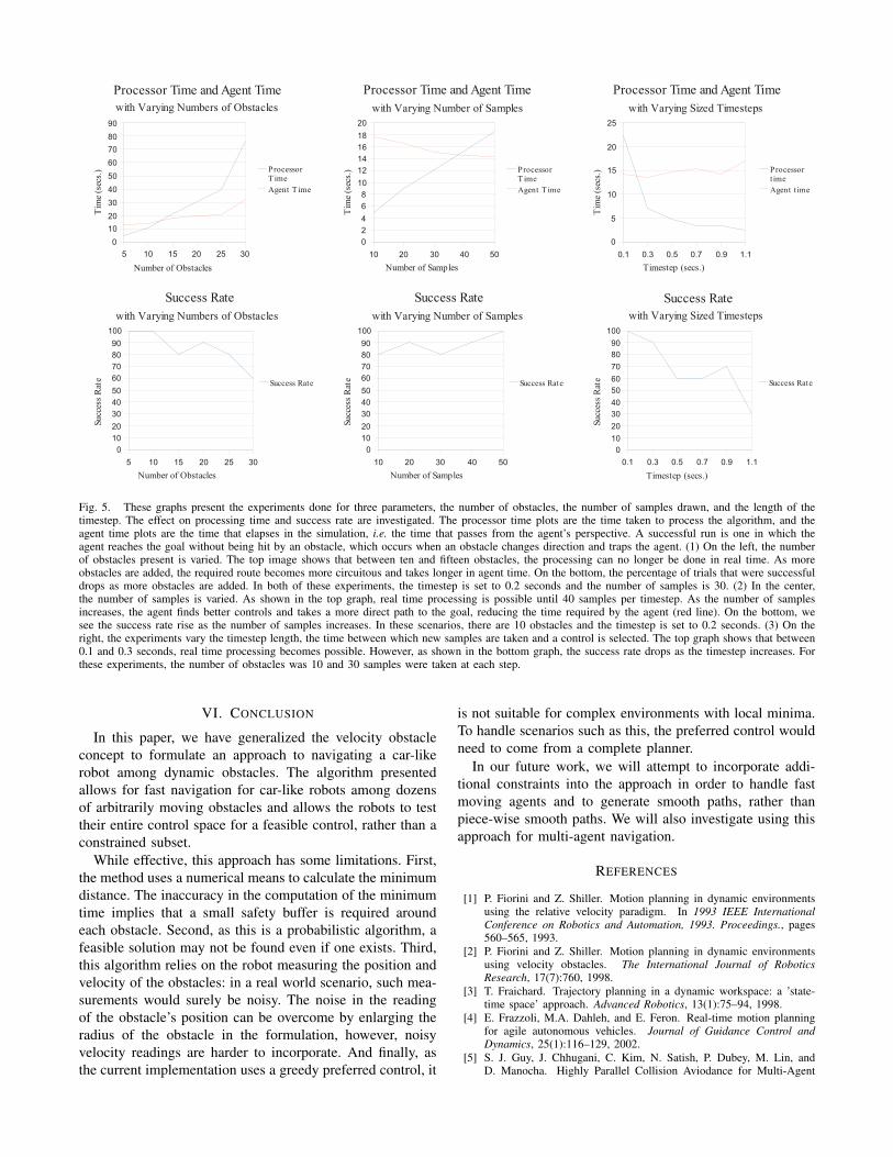
Fig. 5. These graphs present the experiments done for three parameters, the number of obstacles, the number of samples drawn, and the length of thetimestep. The effect on processing time and success rate are investigated. The processor time plots are the time taken to process the algorithm, and theagent time plots are the time that elapses in the simulation, i.e. the time that passes from the agent’s perspective. A successful run is one in which theagent reaches the goal without being hit by an obstacle, which occurs when an obstacle changes direction and traps the agent. (1) On the left, the numberof obstacles present is varied. The top image shows that between ten and fifteen obstacles, the processing can no longer be done in real time. As moreobstacles are added, the required route becomes more circuitous and takes longer in agent time. On the bottom, the percentage of trials that were successfuldrops as more obstacles are added. In both of these experiments, the timestep is set to 0.2 seconds and the number of samples is 30. (2) In the center,the number of samples is varied. As shown in the top graph, real time processing is possible until 40 samples per timestep. As the number of samplesincreases, the agent finds better controls and takes a more direct path to the goal, reducing the time required by the agent (red line). On the bottom, wesee the success rate rise as the number of samples increases. In these scenarios, there are 10 obstacles and the timestep is set to 0.2 seconds. (3) On theright, the experiments vary the timestep length, the time between which new samples are taken and a control is selected. The top graph shows that between0.1 and 0.3 seconds, real time processing becomes possible. However, as shown in the bottom graph, the success rate drops as the timestep increases. Forthese experiments, the number of obstacles was 10 and 30 samples were taken at each step.

VI. CONCLUSION

In this paper, we have generalized the velocity obstacleconcept to formulate an approach to navigating a car-likerobot among dynamic obstacles. The algorithm presentedallows for fast navigation for car-like robots among dozensof arbitrarily moving obstacles and allows the robots to testtheir entire control space for a feasible control, rather than aconstrained subset.

While effective, this approach has some limitations. First,the method uses a numerical means to calculate the minimumdistance. The inaccuracy in the computation of the minimumtime implies that a small safety buffer is required aroundeach obstacle. Second, as this is a probabilistic algorithm, afeasible solution may not be found even if one exists. Third,this algorithm relies on the robot measuring the position andvelocity of the obstacles: in a real world scenario, such mea-surements would surely be noisy. The noise in the readingof the obstacle’s position can be overcome by enlarging theradius of the obstacle in the formulation, however, noisyvelocity readings are harder to incorporate. And finally, asthe current implementation uses a greedy preferred control, it

is not suitable for complex environments with local minima.To handle scenarios such as this, the preferred control wouldneed to come from a complete planner.

In our future work, we will attempt to incorporate addi-tional constraints into the approach in order to handle fastmoving agents and to generate smooth paths, rather thanpiece-wise smooth paths. We will also investigate using thisapproach for multi-agent navigation.

REFERENCES

[1] P. Fiorini and Z. Shiller. Motion planning in dynamic environmentsusing the relative velocity paradigm. In 1993 IEEE InternationalConference on Robotics and Automation, 1993. Proceedings., pages560–565, 1993.

[2] P. Fiorini and Z. Shiller. Motion planning in dynamic environmentsusing velocity obstacles. The International Journal of RoboticsResearch, 17(7):760, 1998.

[3] T. Fraichard. Trajectory planning in a dynamic workspace: a ’state-time space’ approach. Advanced Robotics, 13(1):75–94, 1998.

[4] E. Frazzoli, M.A. Dahleh, and E. Feron. Real-time motion planningfor agile autonomous vehicles. Journal of Guidance Control andDynamics, 25(1):116–129, 2002.

[5] S. J. Guy, J. Chhugani, C. Kim, N. Satish, P. Dubey, M. Lin, andD. Manocha. Highly Parallel Collision Aviodance for Multi-Agent

Simulation. Technical report, Department of Computer Science,University of North Carolina, 2009.

[6] D. Hsu, R. Kindel, J.C. Latombe, and S. Rock. Randomized kino-dynamic motion planning with moving obstacles. The InternationalJournal of Robotics Research, 21(3):233, 2002.

[7] K. Kant and S.W. Zucker. Toward efficient trajectory planning: Thepath-velocity decomposition. The International Journal of RoboticsResearch, 5(3):72, 1986.

[8] O. Khatib. Real-time obstacle avoidance for manipulators and mobilerobots. The International Journal of Robotics Research, 5(1):90, 1986.

[9] F. Lamiraux and J.P. Lammond. Smooth motion planning for car-likevehicles. IEEE Transactions on Robotics and Automation, 17(4):498–501, 2001.

[10] F. Large, D. Vasquez, T. Fraichard, and C. Laugier. Avoiding cars andpedestrians using velocity obstacles and motion prediction. In IEEEIntelligent Vehicle Symposium, pages 375–379, 2004.

[11] J.P. Laumond, PE Jacobs, M. Taix, and RM Murray. A motion plannerfor nonholonomic mobile robots. IEEE Transactions on Robotics andAutomation, 10(5):577–593, 1994.

[12] S.M. LaValle. Planning algorithms. Cambridge University Press,2006.

[13] K. Macek, M. Becker, and R. Siegwart. Motion planning for car-likevehicles in dynamic urban scenarios. In Proc. of the IEEE/RSJ Int.Conf. on Intelligent Robots and Systems (IROS), 2006.

[14] E. Owen and L. Montano. Motion planning in dynamic environmentsusing the velocity space. In 2005 IEEE/RSJ International Conferenceon Intelligent Robots and Systems, 2005.(IROS 2005), pages 2833–2838, 2005.

[15] J. Peng and S. Akella. Coordinating multiple robots with kinody-namic constraints along specified paths. The International Journal ofRobotics Research, 24(4):295, 2005.

[16] S. Petti and T. Fraichard. Safe motion planning in dynamic envi-ronments. In 2005 IEEE/RSJ International Conference on IntelligentRobots and Systems (IROS), pages 2210–2215, 2005.

[17] E. Prassler, J. Scholz, and P. Fiorini. Navigating a robotic wheelchairin a railway station during rush hour. The international journal ofrobotics research, 18(7):711, 1999.

[18] E. Prassler, J. Scholz, and P. Fiorini. A robotics wheelchair forcrowded public environment. IEEE Robotics & Automation Magazine,8(1):38–45, 2001.

[19] Z. Qu, J. Wang, and C.E. Plaisted. A New Analytical Solutionto Mobile Robot Trajectory Generation in the Presence of MovingObstacles. IEEE Transactions on Robotics, 20(6):978–993, 2004.

[20] A. Scheuer, T. Fraichard, and M. INRIA. Continuous-curvature pathplanning for car-like vehicles. In Intelligent Robots and Systems, 1997.IROS’97., Proceedings of the 1997 IEEE/RSJ International Conferenceon, volume 2, 1997.

[21] Z. Shiller, F. Large, and S. Sekhavat. Motion planning in dynamicenvironments: Obstacles moving along arbitrary trajectories. In IEEEInternational Conference on Robotics and Automation, 2001. Proceed-ings 2001 ICRA, volume 4, 2001.

[22] RB Tilove. Local obstacle avoidance for mobile robots based on themethod of artificial potentials. In 1990 IEEE International Conferenceon Robotics and Automation, 1990. Proceedings., pages 566–571,1990.

[23] J. van den Berg, S. J. Guy, M. Lin, and D. Manocha. Reciprocaln-body Collision Avoidance. In International Symposium on RoboticsResearch (ISRR), 2009.

[24] J. Van den Berg, M. Lin, and D. Manocha. Reciprocal VelocityObstacles for real-time multi-agent navigation. In IEEE InternationalConference on Robotics and Automation, 2008. ICRA 2008, pages1928–1935, 2008.

[25] J. van den Berg and M. Overmars. Kinodynamic motion planning onroadmaps in dynamic environments. In Proc. IEEE/RSJ Int. Conf. onIntelligent Robots and Systems-IROS, pages 4253–4258, 2007.

[26] M. Zucker, J. Kuffner, and M. Branicky. Multipartite RRTs for rapidreplanning in dynamic environments. In Proc. IEEE Int. Conf. onRobotics and Automation, pages 1603–1609, 2007.

APPENDIX

In this section, we derive equations used in our approach.The car is modeled as a rigid body moving along a plane,and thus its configuration is (x, y, θ). In the car’s frame ofreference, the origin is at the midpoint of its rear axle and it

is pointed in the positive x direction. In all of our derivations,we assume the wheelbase of the car is 1. To restate (7), thekinematic equations in this reference frame are given as

dx

dt= us cos θ, (11)

dy

dt= us sin θ,

dθ

dt= us tanuφ,

where us and uφ are possible controls in the control spaceU . These are the speed and turning angle, respectively.

We can integrate as follows to derive our equation forA(u, t). First, we integrate dθ

dt ,

θ = us tan(uφ)t. (12)

Next, we integrate dxdt by substituting us tan(uφ)t = θ,

dx

dt= us cos(θ(t)), (13)

= us cos(us tan(uφ)t), (14)∫dx =

∫1

tanuφcos(θ)dθ, (15)

thus, x =1

tanuφsin(us tan(uφ)t). (16)

We can make a similar argument for dydt , and we can

determine from inspection that the integral adds the constant1 to avoid a division by zero. This leads to the equationy = 1

tanuφ(− cos(us tan(uφ)t) + 1). The velocity obstacle

for the simple car and linearly moving obstacle uses thedistance function,

D(u) =

√(sin(us tan(us)t)

tanuφ− pBx − vBxt

)2

(17)

+(−cos(us tan(uφ)t)

tanuφ+

1tanuφ

− pBy − vBy t)2

,

and seeks to find its minimum by searching for a zero in thederivative of D(u)2,

dD(u)2

dt= 2

(sin(us tan(uφ)t)

tanuφ− pBx − vBxt

)(18)

∗(

cos(us tan(uφ)t)us tanuφtanuφ

− vBx)

+2(−cos(us tan(uφ)t)

tanuφ+

1tanuφ

− pBy − vBy t)

∗(

sin(us tan(uφ)t)us tanuφtanuφ

− vBy).

With these defined, we can proceed along the lines ofAlgorithm 1.